research on the civil aero-engine modeling method oriented
TRANSCRIPT
Research on the civil aero-engine modeling methodoriented to control law designShuai Liu
Civil Aviation University of ChinaMing Zhang
Civil Aviation University of ChinaWei Wang ( 918817735qqcom )
Civil Aviation University of ChinaJie Bai
Civil Aviation University of ChinaShiJie Dai
Hebei University of Technology
Research Article
Keywords Aero engine Modeling Control standard model Control law
Posted Date November 9th 2021
DOI httpsdoiorg1021203rs3rs-1029183v1
License This work is licensed under a Creative Commons Attribution 40 International License Read Full License
Research on the civil aero-engine modeling method oriented
to control law design
LIU Shuai1 ZHANG Ming2 WANG Wei1 BAI Jie1 DAI ShiJie3
(1 Key Laboratory for Civil Airworthiness Certification Technology Civil Aviation University of
China Tianjin 300300 China
2 Sino-European Institute of Aviation Engineering Civil Aviation University of China Tianjin
300300 China
3 School of Mechanical Engineering Hebei University of Technology Tianjin 300130 China)
Abstract The non-linear aero-thermal model of civil aero-engine established by the
component method has the characteristics of complex structure and strong coupling of
parameters which is difficult to directly use in the design of control law Aiming at
the problem that civil aero-engine control law design is difficult heavy workload and
can only be used for nominal point linearization model a civil aero-engine modeling
method oriented to control law design is proposed
Simplify the structure according to the aero-engine control function and use
rotor dynamics modeling and combustion reaction dynamics modeling to establish
aero-engine control standard model in differential form which establishes the
corresponding relationship of the parameters required for the control of the
aero-engine full envelope With this control standard model the nonlinear control
method can be directly used in the design of the aero-engine control law which
reduces the workload and difficulty of the control law design to certain extent The
control standard model is established by taking DGEN380 aero-engine as an example
whose accuracy is verified through experiments and an example of the control law
design is given The civil aviation engine modeling method oriented to control law
design has achieved the expected goal Key wordsAero-engineModelingControl standard modelControl law
1 Introduction
The aero-engine control system is used to realize the thrust response of the
aero-engine and ensure that the aero-engine is in a safe state and is an important
system to exert the performance of the aero-engine and ensure the safety of the
aero-engine The aero-engine control system takes its control law as the core The
most critical part in the aero-engine control law design process is the modeling of
aero-engine which takes more than 60 of the controller design time [1]
The component method is recognized in the industry as a modeling method in
the controller design stage The non-linear aero-thermal model of aero-engine is
obtained through component method modeling which has complex structure severe
coupling of various thermal parameters and is difficult to solve so it cannot be
directly used for control law design[2-4] It needs to be linearized at the nominal point
to obtain a linear model in the neighborhood of the nominal point so as to design the
local control algorithm and the global control algorithm
The component method modeling comes from the aero-engine performance
analysis and its model is different from the model required for the design of the civil
aero-engine controller The earliest component method modeling idea was proposed
by Otto and Taylor in the 1950s which solved the problem of performance analysis in
aero-engine design[5] The development of the component method has gone through
the stages of SMOTE code GENENG code and DYNGEN code The National
Aeronautics and Space Administration (NASA) obtained the high-fidelity simulation
code CMAPSS on the basis of the DYNGEN code[6-9] at the beginning of this century
The development process of aero-engine modeling based on the component method is
shown in Figure 1
The component method modeling forms a complete machine-level nonlinear
aero-thermal model through joint working equations with the basis of the
establishment of the aero-thermal relationship of each component of the aero-engine which involves many parameters and can extract the aero-thermal parameters of each
station in real time However large amount of parameters has become barriers to
the design of civil aero-engine controllers Civil aero-engine controls engine thrust
and restricts key parameters by adjusting fuel flow parameters required for
aero-engine control include low-pressure rotor speed that characterizes thrust
high-pressure rotor speed that is safely restricted and turbine temperatureIn other
words not all parameters of each station are required for the control law design So
the model established by the component method differs from the model required for
civil aviation engine control law design The model established by the component
method is strongly nonlinear and includes numerous parameters which are mutual
coupling which directly increases the workload and difficulty of control law design
moreover which affects the architectural form of the civil aero-engine control system
that is local control algorithm with global control algorithm scheduling nominal point
This architectural form cause that many advanced control algorithms (such as sliding
mode variable structure model prediction) only acts on one nominal point of linear
model and cannot reflect the advantages of nonlinear control method
Therefore aiming at control law design this article regards aero-engine as a
power system rather than a collection of components and establishes general civil
aero-engine model which mainly focuses on the necessary parameters required for
control law design has the form of dxdt=f(x)+g(x)u and can be directly used in the of
nonlinear control law design so as to obtain a civil aero-engine modeling method
oriented to the design of control law The model established by this method is named
as aero-engine control standard model
1950 1960 1970 1980 1990 2000 2010
CMAPSS
DYNGEN
GENENGGENENG2
SMOTE
Component Method
Mo
del
Years
Performance Analysis
Figure1 The development process of component method modeling
2civil aero-engine modeling method oriented to control law
design
21 Analysis of Aero-Engine Control Function
The main function of civil aero-engine control is to calculate the fuel flow of the
aero-engine based on the throttle lever angle flight conditions and other parameters to
ensure the thrust level of the aero-engine Among them the aero-engine control
ensuring the thrust level has three meanings (1) maintain the specified thrust value in
the steady state so that it does not change with disturbances (2) ensure that the thrust
changes smoothly within the required time in the transition state (3) ensure that the
limit parameters of the aero-engine do not exceed the limit
It can be known from the civil aero-engine control function that thrust thrust
change rate limit protection parameters and fuel flow are the necessary parameters
for civil aero-engine control law during the control process
22 Aero-engine modeling analysis
The main task of aero-engine control is to control thrust Turbofan engines are
representative of civil aero-engines The thrust of the turbofan engine is mainly
produced by the fan compressed air which produces more than 80 of the total thrust
and the other part is produced by the expansion and acceleration of high temperature
and high pressure gas in the turbine and nozzle The fan is driven by a turbine and the
rotation of the turbine is derived from the high-temperature and high-pressure gas
produced by the compressor and combustion chamber The high-temperature and
high-pressure gas not only makes the turbine rotate with fan to generate thrust but
also expands and accelerates in the turbine to generate thrust Therefore
high-temperature and high-pressure gas is the source of thrust for aero-engines The
established aero-engine model is to describe the mapping relationship between high
temperature and high pressure gas and aero-engine thrust
The low-pressure rotor speed is generally chosen to characterize the thrust of the
civil aero-engine High-temperature and high-pressure of gas originate from the
supercharging process and the combustion process The change of compressor power
can reflect the supercharging process of the air flow and the temperature change in
the combustion chamber can reflect the combustion process of gas and fuel The
combustion reaction kinetic equation is selected to simulate the mixed combustion of
high-pressure airflow and fuel and the temperature change of the combustion
chamber is output The rotor differential term of the rotor dynamics equation is
selected to simulate the change of the rotor speed that is the thrust change The
compressor power term of the rotor dynamics equation simulates the boosting process
of the air flow and the turbine power term can simulate the expansion and
acceleration process of high temperature and high pressure gas and the combustion
reaction dynamics equation is coupled with the rotor dynamics equation through the
outlet temperature parameter of the combustion chamber in the turbine power term
The high-temperature and high-pressure gas is supercharged by the rotation of
the rotor and the temperature increases by fuel combustion but the reason for
maintaining the rotation of the rotor is that the fuel converts chemical energy into
internal energy of the gas that works on the turbine through combustion The aero
engine model designed for the control law needs to describe the mapping relationship
between combustion chamber fuel and low-pressure rotor speed
The general civil turbofan engine structure diagram is shown in Figure 2 The fan
module in the figure includes a booster which is omitted in the figure the dotted
line-number in the figure is the aero-engine position information which is placed at
the aerodynamic parameter corner to indicate the aerodynamic parameter position In
order to enhance the modeling versatility to meet the modeling requirements of the
geared turbofan engine a gear reducer is installed between the low-pressure rotor and
the fan For turbofan engines without gear reducers set the reduction ratio to 1 The
aero-engine in the picture has two shafts a high pressure and a low pressure which
are aerodynamically connected The area of the tail nozzle of the aero-engine is not
adjustable As shown in the figure the fuel is represented by the fuel flow rate Wf
When the fuel enters the combustion chamber of the aero engine the chemical energy
of the fuel is converted into gas internal energy and then the temperature before the
high-pressure turbine T4 rises and the high-pressure turbine changes accordingly
thereby affecting the high-pressure shaft speed N2 next high temperature and high
pressure gas expands in the high-pressure turbine and enters the low-pressure turbine
Because the temperature before the low-pressure turbine T45 is aerodynamically
connected with T4 the change of T45 causes the low-pressure turbine to change
accordingly thereby affecting the low-pressure shaft speed N1 The rotor dynamics
equations of the high-pressure shaft and the low-pressure shaft are established
respectively which are related through the aerodynamic relationship T4=Ф(T45) and
T45 is obtained through the combustion reaction kinetic equation
HP
Compressor
HP
Tuebine LP
Turbine HP Rotor
Fan
Gear
Box
LP Rotor
CombustorInlet
Nozzle
Bypass Duct
Air
Fuel
Air
Gas
N1
N2
4542 25 3 41 44Station 5
Figure2 Civil aero-engine structure diagram
23 Simplification assumptions in modeling
This article only analyzes the idle state climb state cruise state and the
transition process between these states of aero-engine therefore the assumption
condition ignores the aero engine start and stop process Considering the mixed
combustion process of the fuel and high-pressure air flow in the modeling the
combustion reaction kinetic equation is used to describe the combustion process The
reaction mechanism of fuel combustion is involved in the combustion reaction kinetic
modeling most civil aero-engines use Jet A aviation kerosene as fuel so it is assumed
as the aero-engine fuel in the modeling The compressor efficiency turbine efficiency
low-pressure rotor mechanical efficiency and high-pressure rotor mechanical
efficiency are treated as time variables instead of constant value parameters in the
modeling process and fancompressor efficiency turbine efficiency low-pressure
rotor mechanical efficiency and high-pressure rotor mechanical efficiency changing
with the speed of the high-pressurelow-pressure rotor (that is the state of the
compressor and the turbine) is considered Besides the specific heat capacity
parameter is also treated as a variable in the modeling process
24 Aero-engine modeling oriented to control law design
According to the analysis of aero-engine modeling the rotor rotation process and
combustion process are the core of aero-engine modeling The rotor dynamics model
and the combustion reaction dynamics model are established respectively
(1)Rotor dynamics modeling
The rotor of an aero-engine connects the compressor (fan) and the turbine The
rotor dynamics equation establishes the relationship between the rotor speed change
the compressor power (fan power) and the turbine power The rotor dynamics
equation is as formula (1) 1
( )t c
dP P
dt J
= minus (1)
Where t is the time ω is the angular velocity of the rotor J is the moment of
inertia of the rotor Pt is the output power of the turbine Pc is the consumption power
of the compressor Convert the rotor angular velocity in equation (1) into the rotor
speed N then the equation (2) is obtained as follows
2( )30
t c
dNJN P P
dt
= minus (2)
The left side of equation (2) contains all variables related to the rotor the rotors moment of inertia rotor speed and changes of rotor speed the right side is the difference between turbine power and compressor power that is the remaining power of the rotor Equation (2) shows that the product of all variables of the rotor is proportional to the remaining power of the rotor The rotor dynamics equations of the high-pressure rotor and low-pressure rotor are established respectively according to their respective characteristics on the basis of equation (2) as shown in equations (3) and (4) where the subscript L represents low pressure and H represents high pressure
2 HH H HPT HPC( )
30
dNJ N P P
dt
= minus (3)
2 LL L LPT FAN( )
30
dNJ N P P
dt
= minus (4)
According to the aero-thermal relationship formulas (3) and (4) are simplified to obtain formulas (5) and (6) as follows
11 252
cor
2
2 2
corFAN
ln 1[ (1 )( )
e
(e 1)1]
p T L
J f
LPT LT
p F
F
cd NK q W
dt n
c q
n i
= minus +
minusminus
(5)
22 252
corH
25
2
corH
ln 1[ (1 )( )
(e 1)1]
p T H
J f
PT HT
p HC
PC C
cd NK q W
dt n e
c q
n
= minus +
minusminus
(6)
Where
1 1
2
1 1 F
1 1
2
2 2 C
( ) e e30
( ) e30
J LT LT F
J HT HT HC
K J
K J e
minus minus
minus minus
= = =
= = =
(2)Combustion reaction kinetics modeling
The purpose of fuel combustion modeling is to calculate the outlet temperature T4 of the combustor (that is the inlet temperature of the high-pressure turbine) so as to solve the rotor dynamics equation The reaction rate of the fuel is usually ignored in the differential equation of the combustion chamber and T4 is solved by a method of mixing and burning In this paper the fuel reaction rate parameter is introduced into the differential equation of the combustion chamber and the reaction rate is solved by the combustion reaction kinetic equation The differential equation of the combustion chamber is shown in equation (7)
3 3 3 4 4 44
4 4
( LHV)p f f f p
p
c T q W h c T qdT
dt c q
+ + minus= (7)
Where T4 is the exit temperature of the combustion chamber Wf is the fuel flow rate LHV is the low fuel heating value hf is the fuel enthalpy value τ is the residence time constant ωf is the fuel reaction rate whose value is determined by the combustion reaction kinetic equation In this paper ωf is added to the differential equation of the combustor to form equation (7) which aims to consider the influence of fuel combustion on temperature when calculating the outlet temperature of the combustor the main influences include the changing speed of temperature over time temperature value and so on
It can be known from the combustion reaction kinetics that it takes several elementary reactions to decompose the high-carbon mixtures of macromolecules such as aviation kerosene into low-carbon compounds and oxidize low-carbon compounds into products such as carbon dioxide and water The reaction rate ωf of aviation kerosene in the multi-step elementary reaction can be obtained by formula (8)
1
( - )qL
f fi fi i
i
=
= (8)
Where L is the number of elementary reactions and vfirsquorsquovfirsquo are the equivalent coefficients of reactants and products in the i-th elementary combustion reaction of aviation kerosene The reaction rate of aviation kerosene in the i-th elementary reaction can be calculated by equation (9)
1 21 1
q [ ( ) ( ) ]i i
N N
i j jj j
k k
= == minus (9)
Where Χf represents the molar concentration of aviation kerosene k1k2 represent the reaction rate constants of the forward and reverse reactionswhich is determined by the Arrhenius formula The given combustion reaction mechanism is calculated by equation (9) according to the initial conditions of the reaction Assume Jet A aviation kerosene as the fuel and select the C12H23 mechanism[11] as the combustion reaction mechanism of Jet A which includes 16 combustion components and 23 elementary reactions and is given in reference[11]
(3)Aero-engine control standard model
Complete aero-engine high-pressurelow-pressure rotor dynamics modeling combustion reaction dynamics modeling and merge simplify and unify equations in differential forms to form aero-engine control standard model
Establish aero-engine rotor dynamics equations and combustion chamber differential equations and introduce combustion reaction kinetic equations into the combustion chamber differential equations to consider the influence of combustion rate on the outlet temperature of the combustion chamber thus obtaining a aero-engine control standard model which is shown in equations (10)-(14) as follows It can be seen from equation (11) that the model adopts the logarithmic form of the highlow pressure rotor speed which is different from that in the component method so that the simplest model form can be obtained
( ) ( )f gbull= + x x x u (10)
1 2 4[ln ln ]TN N T=x (11) [ ]fW=u (12)
45 2 2252 2 2
cor corFAN
41 25252 2
2 corH corH
3 3
3 44 4
(e 1)1 1 1[ (1 ) ]
e
(e 1)1 1 1( ) [ (1 ) ]
1
p p F
T L
J1 LTLPT F
p p HC
T H
J HTPT PC C
p
p
c c qq
K n n i
c cf q
K en n
c qT T
c q
minus minus minus
minus = minus minus
minus
x
(13)
452
cor
412
2 corH
4 4
1 1 1(1 )
e
1 1 1( ) (1 )
( LHV)
p T L
J1 LTLPT
p T H
J HTPT
f
f
p
cK n
g cK en
h
c q
minus = minus +
x (14)
Ⅲ The application of proposed modeling method
The civil aero-engine modeling method oriented to control law design is used in engine modeling and the model is verified through experiments Figure 3 is an aero engine experimental platform The left side of Figure 3 is a small turbofan engine with a large bypass ratio (DGEN380 aero engine) which is used to verify the model The right side of Figure 3 is the control and monitoring module of the experiment platform
Figure3 Aero-engine test platform
31 Civil aero-engine modeling oriented to control law design
(1) Analysis of characteristic parameters of rotating parts
The characteristic parameters of rotating parts include pressure ratio efficiency flow rate of fancompressor and high pressurelow pressure turbine These characteristic parameters are divided into two parts one is pressure ratio and the other part is flow rate and efficiency The characteristic diagram of aero-engine components show the characteristics of the rotating parts
For the pressure ratio the functional relationship between the rotor speed and the pressure ratio can be fitted by the component experimental data[12] that is πi=f(ni) Equations (15) and (16) respectively give the fitting relationship of low-pressure and high-pressure rotors
4 3 2F LT 1 1 1 1 1 1[ ] [n n n n ]T T = +A C (15)
4 3 2C 2 2 2 2 2 2[ ] [n n n n ]T T
HT = +A C (16)
1 1
2 2
0004758 1777 06332
000191614845 06599
16456 47742 47001 15953 12377
13217 36695 32974 82382 0261
minus = = minus
minus minus = = minus minus minus
A C
Α C
(2)Analysis of mechanical efficiency of high-pressure and low-pressure rotors
Consider the change law of the mechanical efficiency of the high-pressure and low-pressure rotors with its speed The hypothesis of quasi-steady state of the engine state is proposed to calculate the relationship between the mechanical efficiency of the rotor and its rotation speed The quasi-steady state hypothesis of the engine state is that in a certain steady-state neighborhood of the engine when the rotation speed changes slightly the engine power balance equation still holds The mathematical expression of the quasi-steady state hypothesis of the engine state is as equation (17)
0
0
s
t c
N N
S t P P
minus
minus =
(17)
Where Ns represents the steady state speed The relationship curve of the mechanical efficiency of the high-pressurelow-pressure rotor with its speed is obtained according to the quasi-steady state assumption of the engine state
Figure 4 shows the efficiency curve of the DGEN380 aero-engine in which the abscissa represents the relative value of the rotor speed and the ordinate represents the mechanical efficiency of the rotor The trend of mechanical efficiency and speed of the two rotors are similar When the rotation speed is low (the relative value of the rotation speed is less than 06) as the rotation speed increases the mechanical efficiency has a tendency to first decrease and then rise when the rotation speed is high the mechanical efficiency increases with the increase in the rotation speed
04 05 06 07 08 09 10060
065
070
075
080
085
090
095
100
i
ni
High-Pressure Rotor
Low-Pressure Rotor
Figure4 The relationship curve of the mechanical efficiency of the rotor with the relative value of the speed
32 Aero-Engine Control Standard Model of DGEN380
The parameter values are determined through the characteristic parameter analysis of the rotating parts and the mechanical efficiency analysis of the highlow pressure rotor Finally formulas (10)-(14) are obtained and a model that can be directly used for the design of control laws is obtained The model involves rotor dynamics equations and combustion reaction dynamics equations and the time scale of rotor rotation (10-1s) and the time scale of combustion reaction (10-3s-10-5s) are set quite different to consider the differential equations rigidity when solving the model
The ODE15s solver with variable order and multi-step solving is selected to solve the DGEN380 aero-engine control standard model (1)Analysis of steady-state calculation results of model
The control standard model of DGEN380 aero-engine is solved according to the altitude Mach number and fuel flow value corresponding to each state point of the engine given in the manual of DGEN380 aero-engine The state of aero-engine includes idle state (PLA=0deg) cruise state (PLA=43deg) and climb state (PLA=74deg)
Enter the initial condition of equation (10) that is [N10N20T40] and perform a steady-state solution The steady-state solution results are shown in Table 1 The relative error of the model solution value is calculated based on the values given in the manual as shown in Table 1 The maximum error of the steady-state calculation of model is 043 This value indicates that the established DGEN380 aero-engine control standard model can accurately reflect the steady state of the DGEN380 aero-engine
Table1 Steady-state solution results of control standard MS model of DGEN380 N1 relative value N2 relative value T4 relative value
Manual
Value
Simulate
Result
Error
()
Manual
Value
Simulate
Result
Error
()
Manual
Value
Simulate
Result
Error
()
Idle 04701 047006 0009 05676 056761 0002 06516 065154 0009
Cruise 0925 09251 0011 09559 095594 0004 0939 093902 0002
Climb 1 100043 0043 1 100026 0026 1 100034 0034
(2)Analysis of model transition state calculation results
The transition state is solved on the basis of the steady-state solution and the transition curve between each steady-state point of the engine state parameters is obtained Figure 5 shows the aero-engine power spectrum in which the abscissa represents time and the ordinate is the angle of the throttle lever to represent the power state of the aero-engine At the 10th second the throttle lever is quickly pushed from 0deg to 74deg which makes the engine state transition from the idle state to the climb state at the 30th second the throttle lever is retracted to 0deg and the engine state returned to the idle state at the 77th second The throttle lever is quickly pushed from 0deg to 74deg so that the engine state transitions from the idle state to the climb state at the 151st second the throttle lever angle is quickly retracted from 74deg to 43deg and the engine state transitions from the climb state to the cruise state At the 190th second the throttle lever quickly returned to 0deg and the engine state returned to the idle state Figure 6 shows the fuel supply curve corresponding to the engine power spectrum which shows the relationship between the fuel flow rate and time During the experimental H=0m adjust the airflow parameters of the aero engine so that the airflow speed Ma=0338 to ensure that the flight conditions of the model are consistent with the experimental conditions Take the parameter value [N1N2T4] of the idle state as the initial value of the differential equation and then obtain the calculation results of the transition state of the DGEN380 aero-engine control standard mode which are shown in Figure 7-9
0 25 50 75 100 125 150 175 200 2250
10
20
30
40
50
60
70
80
Cruise Power
Climb Power
An
gle
of
PL
A
Deg
ree
Time s
Idle Power
Figure5 Power spectrum diagram of DGEN380
0 25 50 75 100 125 150 175 200 22530
40
50
60
70
80
90
100
110
Fu
el
Flo
w
Kg
h
Time s
Figure6 Fuel supply curve of DGEN380 aero-engine
0 25 50 75 100 125 150 175 200 225045
050
055
060
065
070
075
080
085
090
095
100
105
Model Value
Test Vaule
Climb Power
Cruise Power
N1
Time s
Idle Power
Figure7 Open loop response curve of relative value of low pressure rotor speed
0 25 50 75 100 125 150 175 200 225055
060
065
070
075
080
085
090
095
100
105Climb Power
Cruise Power
Idle Power
Model Value
Test Value
N2
Time s
Figure8 Open-loop response curve of relative value of high-pressure rotor speed
0 25 50 75 100 125 150 175 200 225060
065
070
075
080
085
090
095
100
105
Cruise Power
Idle Power
Model Value
Test Value
Climb Power
T4
Time s
Figure9 Open-loop response curve of the relative value of the outlet temperature of the combustion chamber
23 The example of control law design based on control standard model
Taking the sliding mode variable structure control method as an example design the non-linear control law of aero-engine according to the aero-engine control standard model to realize the thrust control function
The low-pressure rotor speed N1 and the combustion chamber outlet temperature T4 are used as the control parameters and the vector y is set as in equation (18) The control goal is to make the vector y equal to the zero
1 11
4 42
ref
ref
N Ny
T Ty
minus = = minus
y (18)
The parameter index ref in the formula represents the command value The correlation between the input vector of the control standard MS model and the vector y is [1 1] According to the definition of vector y suppose the correlation degree of each sliding function in the sliding mode vector is 1 then the sliding mode vector is set as equation (19)
1 1
2 2
S y
S y
= =
S (19)
The form of the control standard MS model is the normative form to describe the dynamic system According to the control standard MS model the sliding mode vector S has the form of equation (20)
1 2( ) ( )bull= bull + bullS φ φ u (20)
Where function vector φ1() and φ2() are as follows 2
cor
1
4 3 4
4
1 1( )
( )
( ) ( )
LPT m LPT lm Fan m Fan
J1 LPT
m inp V
V
W q W qK n
R T qC C T T
C P V
minus bull = minus minus
φ (21)
2cor
2
44
4
1 1
( )
( )
LPT lm
J1 LPT
V p
V
WK n
R TC C T
C P V
bull =
minus
φ (22)
Considering the influence of uncertainty the function vectors φ1() and φ2() are written as the sum of the nominal value and the uncertain value as shown in equations (23) and (24)
1 1 1N= +φ φ φ (23)
2 2 2N= +φ φ φ (24) Where 1205931N1205932N represent nominal value and Δ1205931Δ1205932 represent uncertain
value Suppose for xisinXtge0then Δ1205931(xt)Δ1205932(xt) satisfy formula (25)
1 (i 12)i
i
= (25)
Set the control law as equation (26) 1 1
1 2N 1 2 2 2 2N 2( ) (I )N
bullminus minus
= minus + + S φ φ φ φ φ φ θ (26)
Set 11 2N 1 2A N
minus= minus S φ φ φ φ 12 2 2N 2B
minus= + S I φ φ It can be seen from equation 243
that SA and SB are bounded so equation (27) holds 0
0
A AM
Bm B BM
t
x X
S S
S S S
(27)
The control goal is to make the sliding mode vector S tend to 0 within a finite time When SA and SB are uncertain and unknown the control input vector θ in the sliding mode is shown in equation (28)
1 1
2 2
( )
( )
K sign S
K sign S
=
θ (28)
Where K1 and K2 are the gain coefficients of the sliding mode control law whose values satisfy formula (29) and λ is positive
AM
Bm
SK
S
+ (29)
The sliding mode control law can satisfy the sliding mode condition
( 0)S S S S S to ensure that the sliding mode vector S tends to 0 within a finite
time Choose λ=0001 to simulate the sliding mode control law according to formula (29) White noises with amplitudes of 00052 and 00042 are added to the low-pressure rotor speed and the outlet temperature of the combustion chamber respectively during the simulation experiment The simulation time is 6s At 0s the aero-engine is stable in the idle state and at 1s the throttle lever is quickly pushed from 0deg to 74deg Figure 10 and Figure 11 show the simulation results of the sliding mode control law
So the design of the aero-engine nonlinear control law is completed The control standard model has a simple form and a standardized format which can be directly used in the design of a sliding mode variable structure controller Under the action of the control input vector the thrust control of the aero-engine can be realized
0 1 2 3 4 5 602
04
06
08
10
12
N1
Time s
Figure10 The response curve of the relative value of the low pressure rotor speed
0 1 2 3 4 5 602
04
06
08
10
12
T4
Time s
Figure11 The response curve of the relative value of the outlet temperature of the combustion chamber
4Conclusion
A civil aviation engine modeling method oriented to control law design is
proposed in this paper Simplify model structure according to aero-engine control function and establish aero-engine control standard model in the differential form through rotor dynamics modeling and combustion reaction dynamics modeling The control standard model directly used in the design of the controller has a small amount of calculation The model establishes the corresponding relationship between the parameters required for the control in the full envelope of the aero-engine and the nonlinear control method can be directly used in the design of the aero-engine control law which simplifies the workload and difficulty of control law design to a certain extent
The civil aero-engine modeling method oriented to control law design establishes the aero-engine control standard model of DGEN380 The maximum error of the model is 043 in the steady state the maximum relative deviation of the model state parameters in transition state is 03516 and the maximum lag time is 008333 seconds Design successfully a nonlinear control law on the basis of the control standard model by taking the sliding mode method as an example The control standard model used in the design of aero-engine control law can simplify the design process reduce the workload and reduce the design difficulty
references
[1] Hanz Richter Advanced Control of Turbofan Engines Cleveland State University Springer2012
[2] Eberle C Gerlinger P Geigle K P et al Numerical investigation of transient soot evolution processes in an aero-engine model combustor[J] Combustion Science and Technology 2015 187(12) 1841-1866
[3] Bai Jie Liu ShuaiWang WeiIdentification method for parameter uncertain model of aero-engine [J] Journal of Aerospace Power202035(01)178-184
[4] Zheng Q Fang J Hu Z et al Aero-engine on-board model based on batch normalize deep neural network[J] IEEE Access 2019 7 54855-54862
[5] Otto E W Taylor B L Dynamics of a Turbojet Engine Considered as a Quasi Static System[R]NACA TN-20911950
[6] Seldner K Generalized simulation technique for turbojet engine system analysis[M] New York National Aeronautics and Space Administration 1972
[7] Szuch R HYDES a generalized hybrid computer program for studying turbojet or turbofan engine dynamics[R] Ohio NASATM 1974
[8] Sellers F Daniele J DYNGEN A program for calculating steady-state and transient performance of turbojet and turbofan engines[M] New York National Aeronautics and Space Administration 1975
[9] Turner G Reed A Ryder R et al Multi-fidelity simulation of a turbofan engine with results zoomed into mini-maps for a zero-d cycle simulation[C]ASME Turbo Expo 2004 Power for Land Sea and Air American Society of Mechanical Engineers Digital Collection 2004 219-230
[10] Wen X Luo Y Luo K et al LES of pulverized coal combustion with a multi-regime flamelet model[J] Fuel 2017 188 661-671
[11] Kundu K Penko P Yang S Reduced reaction mechanisms for numerical calculations in combustion of hydrocarbon fuels[C]36th AIAA Aerospace Sciences Meeting and Exhibit 1998 803
[12] Qian FAbaid N Zuo L Multiple-Scale Analysis of a Tunable Bi-Stable Piezoelectric
Energy Harvester[J] ASME Letters Dyn Sys Control 2021 1(2) 021006 [13] Bhattacharya C Ray A Data-Driven Detection and Classification of Regimes in Chaotic
Systems Via Hidden Markov Modeling[J] ASME Letters Dyn Sys Control 2021 1(2) 021009
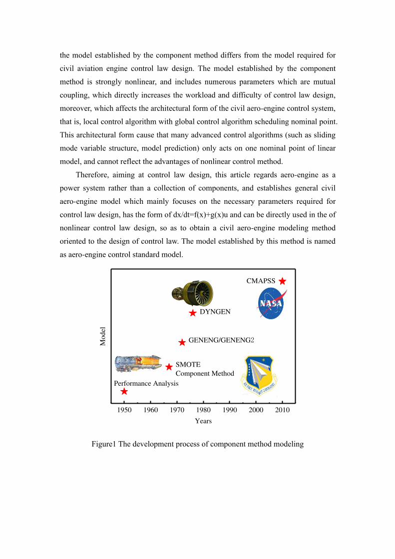
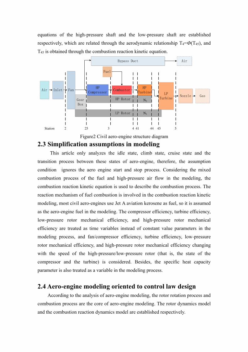
1 1
2
1 1 F
1 1
2
2 2 C
( ) e e30
( ) e30
J LT LT F
J HT HT HC
K J
K J e
minus minus
minus minus
= = =
= = =
(2)Combustion reaction kinetics modeling
The purpose of fuel combustion modeling is to calculate the outlet temperature T4 of the combustor (that is the inlet temperature of the high-pressure turbine) so as to solve the rotor dynamics equation The reaction rate of the fuel is usually ignored in the differential equation of the combustion chamber and T4 is solved by a method of mixing and burning In this paper the fuel reaction rate parameter is introduced into the differential equation of the combustion chamber and the reaction rate is solved by the combustion reaction kinetic equation The differential equation of the combustion chamber is shown in equation (7)
3 3 3 4 4 44
4 4
( LHV)p f f f p
p
c T q W h c T qdT
dt c q
+ + minus= (7)
Where T4 is the exit temperature of the combustion chamber Wf is the fuel flow rate LHV is the low fuel heating value hf is the fuel enthalpy value τ is the residence time constant ωf is the fuel reaction rate whose value is determined by the combustion reaction kinetic equation In this paper ωf is added to the differential equation of the combustor to form equation (7) which aims to consider the influence of fuel combustion on temperature when calculating the outlet temperature of the combustor the main influences include the changing speed of temperature over time temperature value and so on
It can be known from the combustion reaction kinetics that it takes several elementary reactions to decompose the high-carbon mixtures of macromolecules such as aviation kerosene into low-carbon compounds and oxidize low-carbon compounds into products such as carbon dioxide and water The reaction rate ωf of aviation kerosene in the multi-step elementary reaction can be obtained by formula (8)
1
( - )qL
f fi fi i
i
=
= (8)
Where L is the number of elementary reactions and vfirsquorsquovfirsquo are the equivalent coefficients of reactants and products in the i-th elementary combustion reaction of aviation kerosene The reaction rate of aviation kerosene in the i-th elementary reaction can be calculated by equation (9)
1 21 1
q [ ( ) ( ) ]i i
N N
i j jj j
k k
= == minus (9)
Where Χf represents the molar concentration of aviation kerosene k1k2 represent the reaction rate constants of the forward and reverse reactionswhich is determined by the Arrhenius formula The given combustion reaction mechanism is calculated by equation (9) according to the initial conditions of the reaction Assume Jet A aviation kerosene as the fuel and select the C12H23 mechanism[11] as the combustion reaction mechanism of Jet A which includes 16 combustion components and 23 elementary reactions and is given in reference[11]
(3)Aero-engine control standard model
Complete aero-engine high-pressurelow-pressure rotor dynamics modeling combustion reaction dynamics modeling and merge simplify and unify equations in differential forms to form aero-engine control standard model
Establish aero-engine rotor dynamics equations and combustion chamber differential equations and introduce combustion reaction kinetic equations into the combustion chamber differential equations to consider the influence of combustion rate on the outlet temperature of the combustion chamber thus obtaining a aero-engine control standard model which is shown in equations (10)-(14) as follows It can be seen from equation (11) that the model adopts the logarithmic form of the highlow pressure rotor speed which is different from that in the component method so that the simplest model form can be obtained
( ) ( )f gbull= + x x x u (10)
1 2 4[ln ln ]TN N T=x (11) [ ]fW=u (12)
45 2 2252 2 2
cor corFAN
41 25252 2
2 corH corH
3 3
3 44 4
(e 1)1 1 1[ (1 ) ]
e
(e 1)1 1 1( ) [ (1 ) ]
1
p p F
T L
J1 LTLPT F
p p HC
T H
J HTPT PC C
p
p
c c qq
K n n i
c cf q
K en n
c qT T
c q
minus minus minus
minus = minus minus
minus
x
(13)
452
cor
412
2 corH
4 4
1 1 1(1 )
e
1 1 1( ) (1 )
( LHV)
p T L
J1 LTLPT
p T H
J HTPT
f
f
p
cK n
g cK en
h
c q
minus = minus +
x (14)
Ⅲ The application of proposed modeling method
The civil aero-engine modeling method oriented to control law design is used in engine modeling and the model is verified through experiments Figure 3 is an aero engine experimental platform The left side of Figure 3 is a small turbofan engine with a large bypass ratio (DGEN380 aero engine) which is used to verify the model The right side of Figure 3 is the control and monitoring module of the experiment platform
Figure3 Aero-engine test platform
31 Civil aero-engine modeling oriented to control law design
(1) Analysis of characteristic parameters of rotating parts
The characteristic parameters of rotating parts include pressure ratio efficiency flow rate of fancompressor and high pressurelow pressure turbine These characteristic parameters are divided into two parts one is pressure ratio and the other part is flow rate and efficiency The characteristic diagram of aero-engine components show the characteristics of the rotating parts
For the pressure ratio the functional relationship between the rotor speed and the pressure ratio can be fitted by the component experimental data[12] that is πi=f(ni) Equations (15) and (16) respectively give the fitting relationship of low-pressure and high-pressure rotors
4 3 2F LT 1 1 1 1 1 1[ ] [n n n n ]T T = +A C (15)
4 3 2C 2 2 2 2 2 2[ ] [n n n n ]T T
HT = +A C (16)
1 1
2 2
0004758 1777 06332
000191614845 06599
16456 47742 47001 15953 12377
13217 36695 32974 82382 0261
minus = = minus
minus minus = = minus minus minus
A C
Α C
(2)Analysis of mechanical efficiency of high-pressure and low-pressure rotors
Consider the change law of the mechanical efficiency of the high-pressure and low-pressure rotors with its speed The hypothesis of quasi-steady state of the engine state is proposed to calculate the relationship between the mechanical efficiency of the rotor and its rotation speed The quasi-steady state hypothesis of the engine state is that in a certain steady-state neighborhood of the engine when the rotation speed changes slightly the engine power balance equation still holds The mathematical expression of the quasi-steady state hypothesis of the engine state is as equation (17)
0
0
s
t c
N N
S t P P
minus
minus =
(17)
Where Ns represents the steady state speed The relationship curve of the mechanical efficiency of the high-pressurelow-pressure rotor with its speed is obtained according to the quasi-steady state assumption of the engine state
Figure 4 shows the efficiency curve of the DGEN380 aero-engine in which the abscissa represents the relative value of the rotor speed and the ordinate represents the mechanical efficiency of the rotor The trend of mechanical efficiency and speed of the two rotors are similar When the rotation speed is low (the relative value of the rotation speed is less than 06) as the rotation speed increases the mechanical efficiency has a tendency to first decrease and then rise when the rotation speed is high the mechanical efficiency increases with the increase in the rotation speed
04 05 06 07 08 09 10060
065
070
075
080
085
090
095
100
i
ni
High-Pressure Rotor
Low-Pressure Rotor
Figure4 The relationship curve of the mechanical efficiency of the rotor with the relative value of the speed
32 Aero-Engine Control Standard Model of DGEN380
The parameter values are determined through the characteristic parameter analysis of the rotating parts and the mechanical efficiency analysis of the highlow pressure rotor Finally formulas (10)-(14) are obtained and a model that can be directly used for the design of control laws is obtained The model involves rotor dynamics equations and combustion reaction dynamics equations and the time scale of rotor rotation (10-1s) and the time scale of combustion reaction (10-3s-10-5s) are set quite different to consider the differential equations rigidity when solving the model
The ODE15s solver with variable order and multi-step solving is selected to solve the DGEN380 aero-engine control standard model (1)Analysis of steady-state calculation results of model
The control standard model of DGEN380 aero-engine is solved according to the altitude Mach number and fuel flow value corresponding to each state point of the engine given in the manual of DGEN380 aero-engine The state of aero-engine includes idle state (PLA=0deg) cruise state (PLA=43deg) and climb state (PLA=74deg)
Enter the initial condition of equation (10) that is [N10N20T40] and perform a steady-state solution The steady-state solution results are shown in Table 1 The relative error of the model solution value is calculated based on the values given in the manual as shown in Table 1 The maximum error of the steady-state calculation of model is 043 This value indicates that the established DGEN380 aero-engine control standard model can accurately reflect the steady state of the DGEN380 aero-engine
Table1 Steady-state solution results of control standard MS model of DGEN380 N1 relative value N2 relative value T4 relative value
Manual
Value
Simulate
Result
Error
()
Manual
Value
Simulate
Result
Error
()
Manual
Value
Simulate
Result
Error
()
Idle 04701 047006 0009 05676 056761 0002 06516 065154 0009
Cruise 0925 09251 0011 09559 095594 0004 0939 093902 0002
Climb 1 100043 0043 1 100026 0026 1 100034 0034
(2)Analysis of model transition state calculation results
The transition state is solved on the basis of the steady-state solution and the transition curve between each steady-state point of the engine state parameters is obtained Figure 5 shows the aero-engine power spectrum in which the abscissa represents time and the ordinate is the angle of the throttle lever to represent the power state of the aero-engine At the 10th second the throttle lever is quickly pushed from 0deg to 74deg which makes the engine state transition from the idle state to the climb state at the 30th second the throttle lever is retracted to 0deg and the engine state returned to the idle state at the 77th second The throttle lever is quickly pushed from 0deg to 74deg so that the engine state transitions from the idle state to the climb state at the 151st second the throttle lever angle is quickly retracted from 74deg to 43deg and the engine state transitions from the climb state to the cruise state At the 190th second the throttle lever quickly returned to 0deg and the engine state returned to the idle state Figure 6 shows the fuel supply curve corresponding to the engine power spectrum which shows the relationship between the fuel flow rate and time During the experimental H=0m adjust the airflow parameters of the aero engine so that the airflow speed Ma=0338 to ensure that the flight conditions of the model are consistent with the experimental conditions Take the parameter value [N1N2T4] of the idle state as the initial value of the differential equation and then obtain the calculation results of the transition state of the DGEN380 aero-engine control standard mode which are shown in Figure 7-9
0 25 50 75 100 125 150 175 200 2250
10
20
30
40
50
60
70
80
Cruise Power
Climb Power
An
gle
of
PL
A
Deg
ree
Time s
Idle Power
Figure5 Power spectrum diagram of DGEN380
0 25 50 75 100 125 150 175 200 22530
40
50
60
70
80
90
100
110
Fu
el
Flo
w
Kg
h
Time s
Figure6 Fuel supply curve of DGEN380 aero-engine
0 25 50 75 100 125 150 175 200 225045
050
055
060
065
070
075
080
085
090
095
100
105
Model Value
Test Vaule
Climb Power
Cruise Power
N1
Time s
Idle Power
Figure7 Open loop response curve of relative value of low pressure rotor speed
0 25 50 75 100 125 150 175 200 225055
060
065
070
075
080
085
090
095
100
105Climb Power
Cruise Power
Idle Power
Model Value
Test Value
N2
Time s
Figure8 Open-loop response curve of relative value of high-pressure rotor speed
0 25 50 75 100 125 150 175 200 225060
065
070
075
080
085
090
095
100
105
Cruise Power
Idle Power
Model Value
Test Value
Climb Power
T4
Time s
Figure9 Open-loop response curve of the relative value of the outlet temperature of the combustion chamber
23 The example of control law design based on control standard model
Taking the sliding mode variable structure control method as an example design the non-linear control law of aero-engine according to the aero-engine control standard model to realize the thrust control function
The low-pressure rotor speed N1 and the combustion chamber outlet temperature T4 are used as the control parameters and the vector y is set as in equation (18) The control goal is to make the vector y equal to the zero
1 11
4 42
ref
ref
N Ny
T Ty
minus = = minus
y (18)
The parameter index ref in the formula represents the command value The correlation between the input vector of the control standard MS model and the vector y is [1 1] According to the definition of vector y suppose the correlation degree of each sliding function in the sliding mode vector is 1 then the sliding mode vector is set as equation (19)
1 1
2 2
S y
S y
= =
S (19)
The form of the control standard MS model is the normative form to describe the dynamic system According to the control standard MS model the sliding mode vector S has the form of equation (20)
1 2( ) ( )bull= bull + bullS φ φ u (20)
Where function vector φ1() and φ2() are as follows 2
cor
1
4 3 4
4
1 1( )
( )
( ) ( )
LPT m LPT lm Fan m Fan
J1 LPT
m inp V
V
W q W qK n
R T qC C T T
C P V
minus bull = minus minus
φ (21)
2cor
2
44
4
1 1
( )
( )
LPT lm
J1 LPT
V p
V
WK n
R TC C T
C P V
bull =
minus
φ (22)
Considering the influence of uncertainty the function vectors φ1() and φ2() are written as the sum of the nominal value and the uncertain value as shown in equations (23) and (24)
1 1 1N= +φ φ φ (23)
2 2 2N= +φ φ φ (24) Where 1205931N1205932N represent nominal value and Δ1205931Δ1205932 represent uncertain
value Suppose for xisinXtge0then Δ1205931(xt)Δ1205932(xt) satisfy formula (25)
1 (i 12)i
i
= (25)
Set the control law as equation (26) 1 1
1 2N 1 2 2 2 2N 2( ) (I )N
bullminus minus
= minus + + S φ φ φ φ φ φ θ (26)
Set 11 2N 1 2A N
minus= minus S φ φ φ φ 12 2 2N 2B
minus= + S I φ φ It can be seen from equation 243
that SA and SB are bounded so equation (27) holds 0
0
A AM
Bm B BM
t
x X
S S
S S S
(27)
The control goal is to make the sliding mode vector S tend to 0 within a finite time When SA and SB are uncertain and unknown the control input vector θ in the sliding mode is shown in equation (28)
1 1
2 2
( )
( )
K sign S
K sign S
=
θ (28)
Where K1 and K2 are the gain coefficients of the sliding mode control law whose values satisfy formula (29) and λ is positive
AM
Bm
SK
S
+ (29)
The sliding mode control law can satisfy the sliding mode condition
( 0)S S S S S to ensure that the sliding mode vector S tends to 0 within a finite
time Choose λ=0001 to simulate the sliding mode control law according to formula (29) White noises with amplitudes of 00052 and 00042 are added to the low-pressure rotor speed and the outlet temperature of the combustion chamber respectively during the simulation experiment The simulation time is 6s At 0s the aero-engine is stable in the idle state and at 1s the throttle lever is quickly pushed from 0deg to 74deg Figure 10 and Figure 11 show the simulation results of the sliding mode control law
So the design of the aero-engine nonlinear control law is completed The control standard model has a simple form and a standardized format which can be directly used in the design of a sliding mode variable structure controller Under the action of the control input vector the thrust control of the aero-engine can be realized
0 1 2 3 4 5 602
04
06
08
10
12
N1
Time s
Figure10 The response curve of the relative value of the low pressure rotor speed
0 1 2 3 4 5 602
04
06
08
10
12
T4
Time s
Figure11 The response curve of the relative value of the outlet temperature of the combustion chamber
4Conclusion
A civil aviation engine modeling method oriented to control law design is
proposed in this paper Simplify model structure according to aero-engine control function and establish aero-engine control standard model in the differential form through rotor dynamics modeling and combustion reaction dynamics modeling The control standard model directly used in the design of the controller has a small amount of calculation The model establishes the corresponding relationship between the parameters required for the control in the full envelope of the aero-engine and the nonlinear control method can be directly used in the design of the aero-engine control law which simplifies the workload and difficulty of control law design to a certain extent
The civil aero-engine modeling method oriented to control law design establishes the aero-engine control standard model of DGEN380 The maximum error of the model is 043 in the steady state the maximum relative deviation of the model state parameters in transition state is 03516 and the maximum lag time is 008333 seconds Design successfully a nonlinear control law on the basis of the control standard model by taking the sliding mode method as an example The control standard model used in the design of aero-engine control law can simplify the design process reduce the workload and reduce the design difficulty
references
[1] Hanz Richter Advanced Control of Turbofan Engines Cleveland State University Springer2012
[2] Eberle C Gerlinger P Geigle K P et al Numerical investigation of transient soot evolution processes in an aero-engine model combustor[J] Combustion Science and Technology 2015 187(12) 1841-1866
[3] Bai Jie Liu ShuaiWang WeiIdentification method for parameter uncertain model of aero-engine [J] Journal of Aerospace Power202035(01)178-184
[4] Zheng Q Fang J Hu Z et al Aero-engine on-board model based on batch normalize deep neural network[J] IEEE Access 2019 7 54855-54862
[5] Otto E W Taylor B L Dynamics of a Turbojet Engine Considered as a Quasi Static System[R]NACA TN-20911950
[6] Seldner K Generalized simulation technique for turbojet engine system analysis[M] New York National Aeronautics and Space Administration 1972
[7] Szuch R HYDES a generalized hybrid computer program for studying turbojet or turbofan engine dynamics[R] Ohio NASATM 1974
[8] Sellers F Daniele J DYNGEN A program for calculating steady-state and transient performance of turbojet and turbofan engines[M] New York National Aeronautics and Space Administration 1975
[9] Turner G Reed A Ryder R et al Multi-fidelity simulation of a turbofan engine with results zoomed into mini-maps for a zero-d cycle simulation[C]ASME Turbo Expo 2004 Power for Land Sea and Air American Society of Mechanical Engineers Digital Collection 2004 219-230
[10] Wen X Luo Y Luo K et al LES of pulverized coal combustion with a multi-regime flamelet model[J] Fuel 2017 188 661-671
[11] Kundu K Penko P Yang S Reduced reaction mechanisms for numerical calculations in combustion of hydrocarbon fuels[C]36th AIAA Aerospace Sciences Meeting and Exhibit 1998 803
[12] Qian FAbaid N Zuo L Multiple-Scale Analysis of a Tunable Bi-Stable Piezoelectric
Energy Harvester[J] ASME Letters Dyn Sys Control 2021 1(2) 021006 [13] Bhattacharya C Ray A Data-Driven Detection and Classification of Regimes in Chaotic
Systems Via Hidden Markov Modeling[J] ASME Letters Dyn Sys Control 2021 1(2) 021009
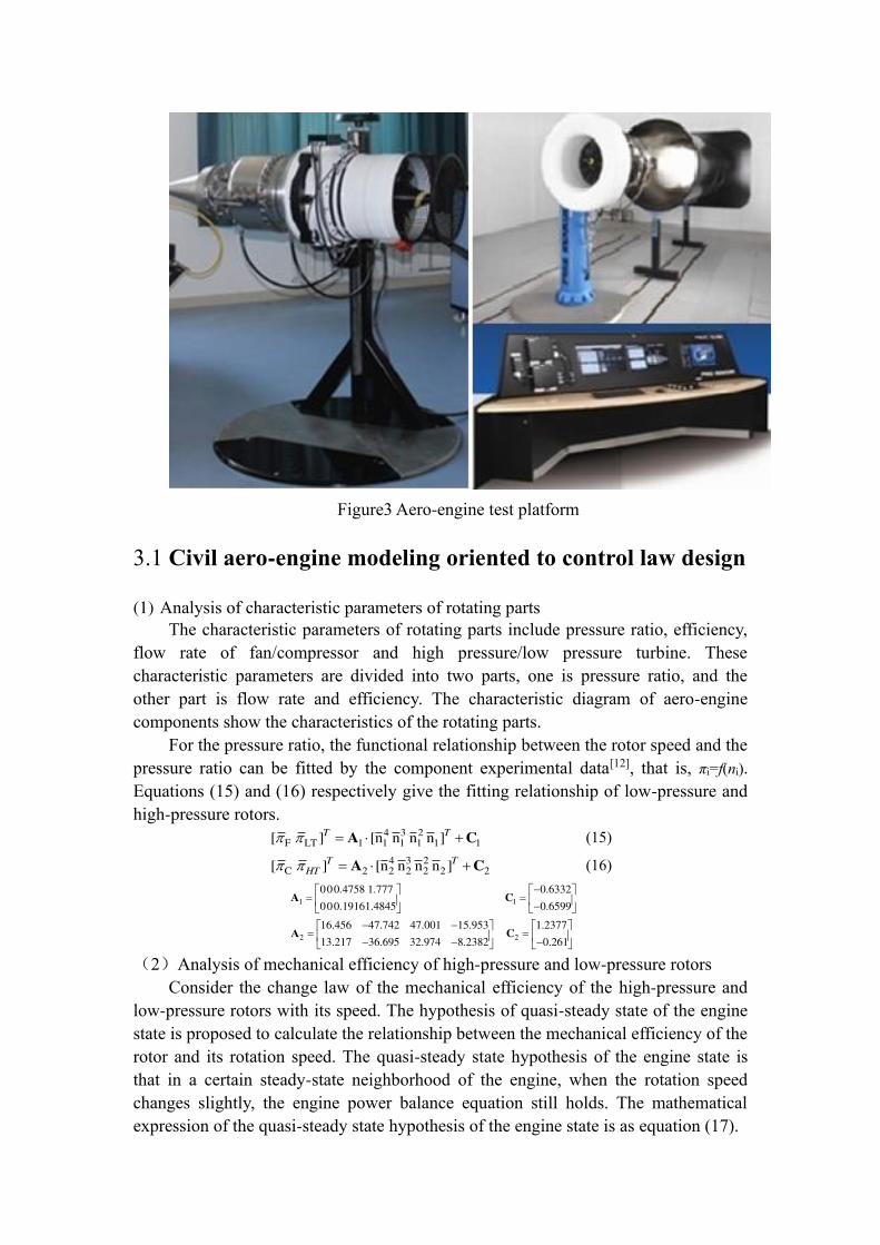

0
0
s
t c
N N
S t P P
minus
minus =
(17)
Where Ns represents the steady state speed The relationship curve of the mechanical efficiency of the high-pressurelow-pressure rotor with its speed is obtained according to the quasi-steady state assumption of the engine state
Figure 4 shows the efficiency curve of the DGEN380 aero-engine in which the abscissa represents the relative value of the rotor speed and the ordinate represents the mechanical efficiency of the rotor The trend of mechanical efficiency and speed of the two rotors are similar When the rotation speed is low (the relative value of the rotation speed is less than 06) as the rotation speed increases the mechanical efficiency has a tendency to first decrease and then rise when the rotation speed is high the mechanical efficiency increases with the increase in the rotation speed
04 05 06 07 08 09 10060
065
070
075
080
085
090
095
100
i
ni
High-Pressure Rotor
Low-Pressure Rotor
Figure4 The relationship curve of the mechanical efficiency of the rotor with the relative value of the speed
32 Aero-Engine Control Standard Model of DGEN380
The parameter values are determined through the characteristic parameter analysis of the rotating parts and the mechanical efficiency analysis of the highlow pressure rotor Finally formulas (10)-(14) are obtained and a model that can be directly used for the design of control laws is obtained The model involves rotor dynamics equations and combustion reaction dynamics equations and the time scale of rotor rotation (10-1s) and the time scale of combustion reaction (10-3s-10-5s) are set quite different to consider the differential equations rigidity when solving the model
The ODE15s solver with variable order and multi-step solving is selected to solve the DGEN380 aero-engine control standard model (1)Analysis of steady-state calculation results of model
The control standard model of DGEN380 aero-engine is solved according to the altitude Mach number and fuel flow value corresponding to each state point of the engine given in the manual of DGEN380 aero-engine The state of aero-engine includes idle state (PLA=0deg) cruise state (PLA=43deg) and climb state (PLA=74deg)
Enter the initial condition of equation (10) that is [N10N20T40] and perform a steady-state solution The steady-state solution results are shown in Table 1 The relative error of the model solution value is calculated based on the values given in the manual as shown in Table 1 The maximum error of the steady-state calculation of model is 043 This value indicates that the established DGEN380 aero-engine control standard model can accurately reflect the steady state of the DGEN380 aero-engine
Table1 Steady-state solution results of control standard MS model of DGEN380 N1 relative value N2 relative value T4 relative value
Manual
Value
Simulate
Result
Error
()
Manual
Value
Simulate
Result
Error
()
Manual
Value
Simulate
Result
Error
()
Idle 04701 047006 0009 05676 056761 0002 06516 065154 0009
Cruise 0925 09251 0011 09559 095594 0004 0939 093902 0002
Climb 1 100043 0043 1 100026 0026 1 100034 0034
(2)Analysis of model transition state calculation results
The transition state is solved on the basis of the steady-state solution and the transition curve between each steady-state point of the engine state parameters is obtained Figure 5 shows the aero-engine power spectrum in which the abscissa represents time and the ordinate is the angle of the throttle lever to represent the power state of the aero-engine At the 10th second the throttle lever is quickly pushed from 0deg to 74deg which makes the engine state transition from the idle state to the climb state at the 30th second the throttle lever is retracted to 0deg and the engine state returned to the idle state at the 77th second The throttle lever is quickly pushed from 0deg to 74deg so that the engine state transitions from the idle state to the climb state at the 151st second the throttle lever angle is quickly retracted from 74deg to 43deg and the engine state transitions from the climb state to the cruise state At the 190th second the throttle lever quickly returned to 0deg and the engine state returned to the idle state Figure 6 shows the fuel supply curve corresponding to the engine power spectrum which shows the relationship between the fuel flow rate and time During the experimental H=0m adjust the airflow parameters of the aero engine so that the airflow speed Ma=0338 to ensure that the flight conditions of the model are consistent with the experimental conditions Take the parameter value [N1N2T4] of the idle state as the initial value of the differential equation and then obtain the calculation results of the transition state of the DGEN380 aero-engine control standard mode which are shown in Figure 7-9
0 25 50 75 100 125 150 175 200 2250
10
20
30
40
50
60
70
80
Cruise Power
Climb Power
An
gle
of
PL
A
Deg
ree
Time s
Idle Power
Figure5 Power spectrum diagram of DGEN380
0 25 50 75 100 125 150 175 200 22530
40
50
60
70
80
90
100
110
Fu
el
Flo
w
Kg
h
Time s
Figure6 Fuel supply curve of DGEN380 aero-engine
0 25 50 75 100 125 150 175 200 225045
050
055
060
065
070
075
080
085
090
095
100
105
Model Value
Test Vaule
Climb Power
Cruise Power
N1
Time s
Idle Power
Figure7 Open loop response curve of relative value of low pressure rotor speed
0 25 50 75 100 125 150 175 200 225055
060
065
070
075
080
085
090
095
100
105Climb Power
Cruise Power
Idle Power
Model Value
Test Value
N2
Time s
Figure8 Open-loop response curve of relative value of high-pressure rotor speed
0 25 50 75 100 125 150 175 200 225060
065
070
075
080
085
090
095
100
105
Cruise Power
Idle Power
Model Value
Test Value
Climb Power
T4
Time s
Figure9 Open-loop response curve of the relative value of the outlet temperature of the combustion chamber
23 The example of control law design based on control standard model
Taking the sliding mode variable structure control method as an example design the non-linear control law of aero-engine according to the aero-engine control standard model to realize the thrust control function
The low-pressure rotor speed N1 and the combustion chamber outlet temperature T4 are used as the control parameters and the vector y is set as in equation (18) The control goal is to make the vector y equal to the zero
1 11
4 42
ref
ref
N Ny
T Ty
minus = = minus
y (18)
The parameter index ref in the formula represents the command value The correlation between the input vector of the control standard MS model and the vector y is [1 1] According to the definition of vector y suppose the correlation degree of each sliding function in the sliding mode vector is 1 then the sliding mode vector is set as equation (19)
1 1
2 2
S y
S y
= =
S (19)
The form of the control standard MS model is the normative form to describe the dynamic system According to the control standard MS model the sliding mode vector S has the form of equation (20)
1 2( ) ( )bull= bull + bullS φ φ u (20)
Where function vector φ1() and φ2() are as follows 2
cor
1
4 3 4
4
1 1( )
( )
( ) ( )
LPT m LPT lm Fan m Fan
J1 LPT
m inp V
V
W q W qK n
R T qC C T T
C P V
minus bull = minus minus
φ (21)
2cor
2
44
4
1 1
( )
( )
LPT lm
J1 LPT
V p
V
WK n
R TC C T
C P V
bull =
minus
φ (22)
Considering the influence of uncertainty the function vectors φ1() and φ2() are written as the sum of the nominal value and the uncertain value as shown in equations (23) and (24)
1 1 1N= +φ φ φ (23)
2 2 2N= +φ φ φ (24) Where 1205931N1205932N represent nominal value and Δ1205931Δ1205932 represent uncertain
value Suppose for xisinXtge0then Δ1205931(xt)Δ1205932(xt) satisfy formula (25)
1 (i 12)i
i
= (25)
Set the control law as equation (26) 1 1
1 2N 1 2 2 2 2N 2( ) (I )N
bullminus minus
= minus + + S φ φ φ φ φ φ θ (26)
Set 11 2N 1 2A N
minus= minus S φ φ φ φ 12 2 2N 2B
minus= + S I φ φ It can be seen from equation 243
that SA and SB are bounded so equation (27) holds 0
0
A AM
Bm B BM
t
x X
S S
S S S
(27)
The control goal is to make the sliding mode vector S tend to 0 within a finite time When SA and SB are uncertain and unknown the control input vector θ in the sliding mode is shown in equation (28)
1 1
2 2
( )
( )
K sign S
K sign S
=
θ (28)
Where K1 and K2 are the gain coefficients of the sliding mode control law whose values satisfy formula (29) and λ is positive
AM
Bm
SK
S
+ (29)
The sliding mode control law can satisfy the sliding mode condition
( 0)S S S S S to ensure that the sliding mode vector S tends to 0 within a finite
time Choose λ=0001 to simulate the sliding mode control law according to formula (29) White noises with amplitudes of 00052 and 00042 are added to the low-pressure rotor speed and the outlet temperature of the combustion chamber respectively during the simulation experiment The simulation time is 6s At 0s the aero-engine is stable in the idle state and at 1s the throttle lever is quickly pushed from 0deg to 74deg Figure 10 and Figure 11 show the simulation results of the sliding mode control law
So the design of the aero-engine nonlinear control law is completed The control standard model has a simple form and a standardized format which can be directly used in the design of a sliding mode variable structure controller Under the action of the control input vector the thrust control of the aero-engine can be realized
0 1 2 3 4 5 602
04
06
08
10
12
N1
Time s
Figure10 The response curve of the relative value of the low pressure rotor speed
0 1 2 3 4 5 602
04
06
08
10
12
T4
Time s
Figure11 The response curve of the relative value of the outlet temperature of the combustion chamber
4Conclusion
A civil aviation engine modeling method oriented to control law design is
proposed in this paper Simplify model structure according to aero-engine control function and establish aero-engine control standard model in the differential form through rotor dynamics modeling and combustion reaction dynamics modeling The control standard model directly used in the design of the controller has a small amount of calculation The model establishes the corresponding relationship between the parameters required for the control in the full envelope of the aero-engine and the nonlinear control method can be directly used in the design of the aero-engine control law which simplifies the workload and difficulty of control law design to a certain extent
The civil aero-engine modeling method oriented to control law design establishes the aero-engine control standard model of DGEN380 The maximum error of the model is 043 in the steady state the maximum relative deviation of the model state parameters in transition state is 03516 and the maximum lag time is 008333 seconds Design successfully a nonlinear control law on the basis of the control standard model by taking the sliding mode method as an example The control standard model used in the design of aero-engine control law can simplify the design process reduce the workload and reduce the design difficulty
references
[1] Hanz Richter Advanced Control of Turbofan Engines Cleveland State University Springer2012
[2] Eberle C Gerlinger P Geigle K P et al Numerical investigation of transient soot evolution processes in an aero-engine model combustor[J] Combustion Science and Technology 2015 187(12) 1841-1866
[3] Bai Jie Liu ShuaiWang WeiIdentification method for parameter uncertain model of aero-engine [J] Journal of Aerospace Power202035(01)178-184
[4] Zheng Q Fang J Hu Z et al Aero-engine on-board model based on batch normalize deep neural network[J] IEEE Access 2019 7 54855-54862
[5] Otto E W Taylor B L Dynamics of a Turbojet Engine Considered as a Quasi Static System[R]NACA TN-20911950
[6] Seldner K Generalized simulation technique for turbojet engine system analysis[M] New York National Aeronautics and Space Administration 1972
[7] Szuch R HYDES a generalized hybrid computer program for studying turbojet or turbofan engine dynamics[R] Ohio NASATM 1974
[8] Sellers F Daniele J DYNGEN A program for calculating steady-state and transient performance of turbojet and turbofan engines[M] New York National Aeronautics and Space Administration 1975
[9] Turner G Reed A Ryder R et al Multi-fidelity simulation of a turbofan engine with results zoomed into mini-maps for a zero-d cycle simulation[C]ASME Turbo Expo 2004 Power for Land Sea and Air American Society of Mechanical Engineers Digital Collection 2004 219-230
[10] Wen X Luo Y Luo K et al LES of pulverized coal combustion with a multi-regime flamelet model[J] Fuel 2017 188 661-671
[11] Kundu K Penko P Yang S Reduced reaction mechanisms for numerical calculations in combustion of hydrocarbon fuels[C]36th AIAA Aerospace Sciences Meeting and Exhibit 1998 803
[12] Qian FAbaid N Zuo L Multiple-Scale Analysis of a Tunable Bi-Stable Piezoelectric
Energy Harvester[J] ASME Letters Dyn Sys Control 2021 1(2) 021006 [13] Bhattacharya C Ray A Data-Driven Detection and Classification of Regimes in Chaotic
Systems Via Hidden Markov Modeling[J] ASME Letters Dyn Sys Control 2021 1(2) 021009
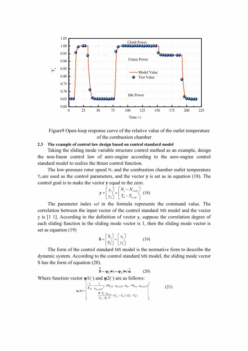

0 1 2 3 4 5 602
04
06
08
10
12
N1
Time s
Figure10 The response curve of the relative value of the low pressure rotor speed
0 1 2 3 4 5 602
04
06
08
10
12
T4
Time s
Figure11 The response curve of the relative value of the outlet temperature of the combustion chamber
4Conclusion
A civil aviation engine modeling method oriented to control law design is
proposed in this paper Simplify model structure according to aero-engine control function and establish aero-engine control standard model in the differential form through rotor dynamics modeling and combustion reaction dynamics modeling The control standard model directly used in the design of the controller has a small amount of calculation The model establishes the corresponding relationship between the parameters required for the control in the full envelope of the aero-engine and the nonlinear control method can be directly used in the design of the aero-engine control law which simplifies the workload and difficulty of control law design to a certain extent
The civil aero-engine modeling method oriented to control law design establishes the aero-engine control standard model of DGEN380 The maximum error of the model is 043 in the steady state the maximum relative deviation of the model state parameters in transition state is 03516 and the maximum lag time is 008333 seconds Design successfully a nonlinear control law on the basis of the control standard model by taking the sliding mode method as an example The control standard model used in the design of aero-engine control law can simplify the design process reduce the workload and reduce the design difficulty
references
[1] Hanz Richter Advanced Control of Turbofan Engines Cleveland State University Springer2012
[2] Eberle C Gerlinger P Geigle K P et al Numerical investigation of transient soot evolution processes in an aero-engine model combustor[J] Combustion Science and Technology 2015 187(12) 1841-1866
[3] Bai Jie Liu ShuaiWang WeiIdentification method for parameter uncertain model of aero-engine [J] Journal of Aerospace Power202035(01)178-184
[4] Zheng Q Fang J Hu Z et al Aero-engine on-board model based on batch normalize deep neural network[J] IEEE Access 2019 7 54855-54862
[5] Otto E W Taylor B L Dynamics of a Turbojet Engine Considered as a Quasi Static System[R]NACA TN-20911950
[6] Seldner K Generalized simulation technique for turbojet engine system analysis[M] New York National Aeronautics and Space Administration 1972
[7] Szuch R HYDES a generalized hybrid computer program for studying turbojet or turbofan engine dynamics[R] Ohio NASATM 1974
[8] Sellers F Daniele J DYNGEN A program for calculating steady-state and transient performance of turbojet and turbofan engines[M] New York National Aeronautics and Space Administration 1975
[9] Turner G Reed A Ryder R et al Multi-fidelity simulation of a turbofan engine with results zoomed into mini-maps for a zero-d cycle simulation[C]ASME Turbo Expo 2004 Power for Land Sea and Air American Society of Mechanical Engineers Digital Collection 2004 219-230
[10] Wen X Luo Y Luo K et al LES of pulverized coal combustion with a multi-regime flamelet model[J] Fuel 2017 188 661-671
[11] Kundu K Penko P Yang S Reduced reaction mechanisms for numerical calculations in combustion of hydrocarbon fuels[C]36th AIAA Aerospace Sciences Meeting and Exhibit 1998 803
[12] Qian FAbaid N Zuo L Multiple-Scale Analysis of a Tunable Bi-Stable Piezoelectric
Energy Harvester[J] ASME Letters Dyn Sys Control 2021 1(2) 021006 [13] Bhattacharya C Ray A Data-Driven Detection and Classification of Regimes in Chaotic
Systems Via Hidden Markov Modeling[J] ASME Letters Dyn Sys Control 2021 1(2) 021009

Energy Harvester[J] ASME Letters Dyn Sys Control 2021 1(2) 021006 [13] Bhattacharya C Ray A Data-Driven Detection and Classification of Regimes in Chaotic
Systems Via Hidden Markov Modeling[J] ASME Letters Dyn Sys Control 2021 1(2) 021009