PO

LIT

ICA

L E

CO

NO

MY

R

ESEA

RC

H IN

ST

ITU

TE

Engel’s Law Around the World 150 Years Later

Richard Anker

January 2011

WORKINGPAPER SERIES

Number 247

Gordon Hall

418 North Pleasant Street

Amherst, MA 01002

Phone: 413.545.6355

Fax: 413.577.0261

peri@econs.umass.edu

www.umass.edu/peri/

Engel’s law around the world 150 years later

Acknowledgements I would like to thank Guy Standing, Joe Ritter and James Heinz for their valuable comments and suggestions and Valentina Stoevska for help in providing data and clarifying concepts. As usual though, my wife Martha deserves the greatest thanks for her suggestions, input and help. 1.0 Introduction One of the most enduring relationships in economics is that proposed by Ernst Engel in 1857. Even today, it is often referred to as a law, “Engel’s law”.

“The poorer is a family, the greater is the proportion of the total outgo [family expen-ditures] which must be used for food. … The proportion of the outgo used for food, other things being equal is the best measure of the material standard of living of a population.” (Engel quoted in Zimmerman, 1932)

The 150th anniversary of Engel’s law passed in 2007. With this in mind, the present paper looks at the extent to which Engel’s law is relevant in today’s world by looking across coun-tries at the relationship between the share of household expenditure spent on food and na-tional income per capita. Investigating the relevance of Engel’s law is not just of historical interest. Poverty reduction is arguably the most important objective of the United Nations’ Millennium Development Goals as well as of national policy in many countries - - and the food share of household ex-penditure is often used to measure national poverty lines and therefore help determine na-tional poverty rates.1 It is also possible to argue that the 2008 financial crisis, which was caused by a bubble in American house prices, was inevitable because the proportion of ex-penditure for a major item such as housing, or food, is not sustainable when it far exceeds historic norms (Shiller, 2008; Interest.com). This paper provides an empirical analysis of Engel’s aw based on data for almost every coun-try and territory in the world. The paper is structured as follows. Section 2 reviews how the view of Engel’s law has evolved over the past 150 years. Section 3 describes the data used in the cross-national empirical analysis. It begins with a description of how data on the food share of household expenditure was collected. This includes discussion of the international standard classification for household expenditure; sources used to find national estimates; and aspects which reduce cross-country comparability of national food share estimates (de-

1 The most common methodology to calculate a national poverty line is to divide the cost of a nutritionally acceptable diet by the food share of household expenditures. A wide range of countries use this approach to estimate their national poverty line including United States (Orshansky, 1969); Philippines, Thailand, and Vietnam in Asia (Asra and Santos-Francisco, 2001); and many Latin American countries (Sainz, 1994).

1

pendant variable in cross-national analysis) and income per capita in purchasing power parity units (main explanatory variable in cross-national analysis). Section 4 is concerned with ana-lytical issues. Section 5 begins the empirical analysis with an analysis of household income and expenditure survey data tabulated by income decile for 46 countries or territories to ob-serve if Engel’s law still operates today at the household level within countries. The cross-national analysis of national level data in Section 6 begins with scatterplots and descriptive statistics, and goes on to a multivariate regression analysis. Section 7 provides conclusions. Appendix A investigates the relationship between food share and expenditure for food taken away from home, since the latter should reduce the former. A feature of this paper is that it is based on data for almost all countries and territories in the world (207), many more than in previous studies have used. This facilitates analysis of the relationship between the food share of household expenditure and national income per capita, especially how this differs by development level. Other distinguishing features of this paper compared to previous cross-national studies are that: national food share estimates are from national statistical offices based almost exclusively on household budget surveys and not es-timates from international organizations or SNA statistics; expenditures for alcohol, tobacco and food taken away from home are excluded from reported food expenditure whenever a national statistical office included these in food expenditure; income per capita in PPP and food expenditure are measured for the same year; and newly revised and improved World Bank estimates of GDP per capita in PPP are used to measure national material standard of living. In contrast, previous cross-national studies have often: used food expenditure as re-ported by national authorities or international organizations even though alcohol, tobacco and food taken away from home are often included in reported food expenditure; used food share estimates based on SNA statistics that include all expenditure by individuals in a country re-gardless of whether they are by tourists, cross-border persons or residents; been based on data for different years for food share and per capita income, because countries always use data from an earlier year to estimate food share and often a much earlier year; and did not have access to the newly revised and improved World Bank estimates of GDP per capita in PPP. It was possible to find data on the food share of household expenditure for virtually every country and territory in the world, because household expenditure weights (including of course percent for food) are required to calculate CPI (consumer price index) and CPI is an essential tool of economic and policy. It is highly unusual to have an economic variable with national values for almost every country and territory in the world estimated by national sta-tistical offices. This has important advantages, because national statistical offices understand local conditions and base expenditure share estimates on local data. Much more typical when national values are available for an economic variable for almost all countries and territories in the world is for these values to have been estimated by an international organization such as UN, ILO or World Bank. The disadvantage of using estimates from national offices is that this reduces cross-national comparability, because national statistical offices use different methodologies and definitions. For this reason, considerable effort was put into improving cross-country comparability of national food share data as well as to take into consideration in the cross-national analysis differences in national practices as regards measurement of food share.

2

2.0 Historical background of Engel’s law In 1857, Ernst Engel argued that there is a relationship between food expenditure and income using data for 36 European households provided by Le Play and 199 Belgium households provided by Ducpetiaux. As Engels put it, “They delivered the pearls but not the string” (Engel 1857 quoted in Perthel 1975). Engel found an extremely consistent relationship across households between the food share of household expenditure and household income. Perthel (1975) was able to obtain an R2 of .9998 for the LePlay data set, and an R2 of .76 for all 235 households (with an R2 of .998 when data were aggregated into seven groups). Income elas-ticity of food expenditure was .86 for each data set. Although Engel probably massaged his data sets to obtain a more regular relationship between food expenditure and income than ex-isted in the original data (Perthel, 1975), as such fits do not occur in micro household data (e.g. food share of household expenditure increases with income across all 29 households in the Le Play data), Engel’s law took hold in economics. By 1875, Engel’s law had passed over the Atlantic, receiving confirmation and anointment. Wright (1875) waxed “The remarkable harmony in the items of expenditure [between Massa-chusetts, and Europe] shown by percentage of total expenditure must establish the soundness of the economic law pronounced by Dr. Engel.” As head of the Massachusetts Bureau of La-bor Statistics (and later first commissioner of the Bureau of Labor Statistics for the United States), Wright was not content to stop at food expenditure like Engel, and stated that the percentage of household expenditure for clothing (constant), housing (constant), and sundries (increased) also varied with income in accordance with Engel’s law. There was no place for ambivalence as regards Engel’s law or laws at this point in time. On the 75th anniversary of Engel’s law, a review article by Zimmerman (1932) indicates that Engel’s law continued to retain its importance as this article begins by saying: “In the field of family consumption and expenditures, one theory attracts first attention above all others – the so-called Engel’s law.” There is, however, now considerable skepticism about the reach and universality of Engel’s law. Zimmerman hammers home the point that Engel was only con-cerned with the relationship between food expenditure and income (being greatly influenced by the idea of arithmetic and geometric progressions of Malthus, with food expenditure in-creasing at an arithmetic rate and sundry expenditures at a geometric rate), and that others had inappropriately attributed to Engel additional laws on the relationship of non-food items to income. Zimmerman also discusses at length why Engel’s law is not universal across all household, countries, and time periods and concludes that: “It is evident that Engel’s law, rig-idly interpreted [i.e. food share falls with increased household income], is not true for particu-lar families, for particular times, and under certain circumstances,” and that “The ‘Engel’ type of standard of living [i.e. food share of household expenditures] applies to no more than half of the people of the globe.” 2 To explain exceptions to Engel’s law, Zimmerman mentions dif-ferences in personal tastes, cultural preferences, family size, and changes in the types of food purchased. By 1932 then, Engel’s law was still considered very important both as a relation-

2 At the same time, Zimmerman (1932) also concluded that the amount of food expenditures always increases with an increase in income: “The studies made so far indicate that food expenditures nearly always increase with increased expenditure. … I know of no exceptions to this rule. It is one of the elementary and important laws of living.”

3

ship and as an essential measure of welfare. At the same time, it was being questioned based in large part on household budget survey data that were just then becoming widely available. 3 On the centenary of Engel’s law in 1957, a review article by Houthakker (1957) continued to indicate that Engel’s law occupied a central place in economics. The first few sentences read: “Few dates in the history of econometrics are more significant than 1857. In that year, Ernst Engel (1821-1896) published a study in which he formulated an empirical law concerning the relationship between income and expenditure on food. Engel’s law, as it has since become known, states that the proportion of income spent on food declines as income increase.” Dis-cussion in 1957 has now shifted to empirical analysis and statistical confirmation.4 Also changed from 25 years earlier is any discussion that Engel’s law relates to only food expendi-ture, a point emphasized in Zimmerman’s 1932 review. Engel’s law is now considered to be a series of laws. Houthakker (1957) devotes most of his review article to estimating house-hold income elasticities for food, clothing, housing, and miscellaneous items using data from approximately 40 household surveys and 30 countries. Because it is now accepted that household income or expenditure is not the only determinant of the food share of household expenditures, Houthakker controls for family size in regressions as well as points out that his results may have been affected by other factors that were not controled for such as relative prices. He finds that “The elasticities are found to be similar but not equal [across surveys]. Engel’s law, formulated in 1857, is confirmed by all surveys. … To return to the problem of development planning: If no data on the expenditure patterns of a country are available at all, one would not be very far astray by putting the partial elasticity at 0.6 with respect to food.” Since 1957, analyses of food expenditure patterns have become mainly empirical using in-creasingly sophisticated statistical models, in part made possible by an explosion in the avail-ability of household budget data around the world. It is now common for empirical studies of household expenditures to simultaneously analyze how different types of expenditures vary along with household income or total expenditure (unlike Houthakker who analyzed each type of expenditure separately in 1957). Empirical analysis of household expenditures now routinely control for non-income factors that affect the food share of household expenditures such as prices and family size. And it is now conventional wisdom that the income elasticity of food expenditure is less than 1.0 and therefore the food share of household expenditure falls with income. Perhaps for this reason, Engel’s law is now mainly referred to as an his-torical curiosity in the introduction section of papers. Recent work on household expenditure patterns has been based almost always on household data. There have been relatively few cross-national studies of the extent to which Engel’s law remains relevant across countries in the 21st century. A notable exception is a study by Seale and Regmi (2006) that simultaneously estimated parameters for nine expenditure groups with food as one of these groups. They found that the income elasticity of food expenditure fell from about .7 for low income countries to .6, .5 and .1 to .3 for lower middle income, upper middle income and high income countries respectively. This study differs from the present 3 ILO’s International Labor Review, for example, published between 1929 and 1936 many articles based on family budget enquiries because of an increasing interest in the welfare and standard of living of workers around the world. This included, among others, articles on Belgium, Ceylon, China, Denmark, England, Finland, Germany, India, Japan, Malaysia, South Africa, Russia, Sweden, and United States. 4 Houthakker was himself a major player in this empirical analysis, as the Prais and Houthakker (1955) detailed analy-sis of British household expenditure data is a classic in this field.

4

study is several ways. They used data for 114 countries whereas the present study uses data for 207 countries. They dropped 23 countries from their analysis based on regression residu-als, whereas this is not done in the present study. They included alcohol and tobacco expendi-ture in food expenditure because these were included in the ICP food expenditure data they used, whereas the present study excludes alcohol and tobacco expenditure. Their expenditure estimates are often based on SNA statistics and so based on all expenditure on a territory and not just on expenditure of resident households whereas the food expenditure estimates used in the present study are almost always based on household budget survey data. They did not explicitly consider, in contrast to the present study, frequent difference between year of CPI expenditure weight estimates and data year of expenditure data on which they are based; or whether data were national or for urban areas only; or whether food expenditure included ex-penditure for food away from home; or take into consideration distribution of household in-come; or if a country is a transition economy. They did, however, use more sophisticated statistical estimation models than the present study and included prices as an explanatory variable whereas the present study does not. This paper, then, investigates the following questions related to Engel’s law. Does the food share of household expenditure in countries decrease as national per capita income increases; if so does this occur at all development levels and in all parts of the world? And is the food share of household expenditure a good measure of the material standard of living of countries in the 21st century in all parts of the world and at all development levels? 3.0 Data This section describes data used in the cross-national empirical analysis in Section 6. It be-gins with a description of how national food share of household expenditure estimates were gathered and aspects of these data that might affect cross-national comparability. It goes on to describe how income per capita in PPP and other explanatory variables are measured and how measurement of PPP might affect the cross-national empirical results in Section 6. 3.1 Recent national estimates of food share of household expenditure Data for 207 countries or territories on the food share of household expenditure are used in the cross-national analysis in this paper to observe if Engel’s law is relevant today across countries along with economic development and increasing per capita income. Also, data from 46 national household income and expenditure surveys tabulated by income decile are used to confirm that Engel’s law is still relevant today at the household level within coun-tries. Data on food share of household expenditure are available for virtually every country and territory in the world, because tracking inflation is universally considered an essential tool of economic and monetary policy, and household expenditure weights for a fixed basket of goods and services are required to calculate CPI (with food one of the main components in this basket).5 Availability of data for almost every country and territory is a great advantage

5 Inflation is calculated by dividing the average price of a fixed basket of goods and services (i.e. fixed set of expendi-ture weights or shares) in period t+1 by the average price for this basket in period t.

5

for investigating whether the relationship between the food share of household expenditure and national income per capita differs by development level. National estimates of the food share of household expenditure were almost exclusively drawn from official government statistics used to calculate CPI. I started with large ILO and IMF data bases, which included information on household expenditure weights countries and terri-tories used to calculate national CPI. 6 I was given access to country files kept in ILO’s Ge-neva headquarters that contain national information and publications on CPI expenditure weights sent to ILO over the past couple of decades in response to an annual ILO request for such information. There was also an ILO (2007) online metadata with national CPI statistics and information including expenditure weights for 177 countries and territories, although the usefulness of this ILO metadata is limited because it is somewhat out-of-date as it is based on information from an ILO (1992) publication supplemented by an ILO (1999) publication for transition economy countries. There was also an online IMF (2007) online metadata of CPI statistics and information for 75 countries and territories that often included national expendi-ture weights used to estimate CPI. National food share estimates from these three ILO and IMF databases were supplemented primarily by searching national statistical office web sites using a list of web site links pro-vided by ILO. National statistical web sites of well over 100 countries and territories were searched - - whenever recent food expenditure weights were not available in any of the three ILO or IMF databases, or estimates from these three databases were inconsistent or problem-atic in some way. Finally, miscellaneous sources were used for 10 countries or territories for which I still did not have a recent estimate of the food share of household expenditure. 7 All together, an estimate of food share of household expenditure was found for 207 of the 229 countries and territories in the world and 99 percent of the world’s population.8 In the process of putting together the data set on food shares, I often ended up with estimates for different years and/or multiple estimates for one year for countries and territories.9 When this happened, the following rules were used to choose a national estimate. First, the most

6 ILO and IMF are the two international organizations especially concerned with and responsible for CPI statistics. ILO has a mandate from the international statistical community for CPI statistics, sets international statistical standards on how to measure CPI, publishes manuals on CPI measurement, provides technical assistance to countries interested in improving CPI statistics, and requests countries to send it information on CPI (including information on expenditure weights). IMF has an interest in price stability and encourages and assists developing and transition economy countries to improve CPI statistics. Both organizations regularly report and publish national CPI estimates. 7 Miscellaneous sources were regional organization databases for 7 countries or territories (2 from AFRISTAT (2001), 3 from OECD (2007), 2 from European Central Bank (Herrmann and Polgar, 2007), 2 from ICP, International Compa-rability Program (World Bank, 2008a), and 1 from an ILO (2007) online database of national household income and expenditure surveys. 8 I did not find an estimate of the food share of household expenditures for the following: Cuba, Dominican Republic, Eritrea, Guernsey, Holy See, Korea Democratic Republic, Lichtenstein, Libya, Micronesia, Monaco, Nauru, Northern Marianas, Palau, Tokelau, Turkmenistan, Turks and Caicos, Uzbekistan, and Western Sahara. There were also four countries or territories for whom I found an estimate from ILO (1992) that I did not use, because this estimate was ei-ther based on an unrepresentative sample (low income households in Vanuatu) or felt to be too old (Liberia 1963-64; Guyana, 1969-70; Falkland Islands, 1971). 9 For example, I found the following regional databases of national CPI expenditure weights: (i) EUROSTAT (2008) harmonized database for 30 countries; (ii) OECD (2007) metadata for 32 countries; (iii) MERCOSUR and Chile har-monized data for 5 South American countries (IBGE, 2007); (iv) AFRISTAT (2001) harmonized database for 10 West African countries; (v) European Central Bank data for 9 South-East European countries (Herrmann and Polgar, 2007); and (vi) ICP database for 120 countries (World Bank, 2008a).

6

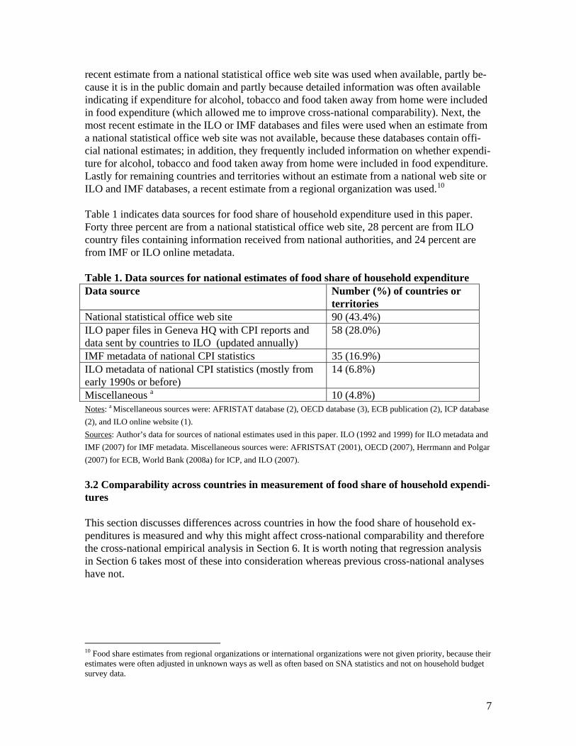
recent estimate from a national statistical office web site was used when available, partly be-cause it is in the public domain and partly because detailed information was often available indicating if expenditure for alcohol, tobacco and food taken away from home were included in food expenditure (which allowed me to improve cross-national comparability). Next, the most recent estimate in the ILO or IMF databases and files were used when an estimate from a national statistical office web site was not available, because these databases contain offi-cial national estimates; in addition, they frequently included information on whether expendi-ture for alcohol, tobacco and food taken away from home were included in food expenditure. Lastly for remaining countries and territories without an estimate from a national web site or ILO and IMF databases, a recent estimate from a regional organization was used.10 Table 1 indicates data sources for food share of household expenditure used in this paper. Forty three percent are from a national statistical office web site, 28 percent are from ILO country files containing information received from national authorities, and 24 percent are from IMF or ILO online metadata. Table 1. Data sources for national estimates of food share of household expenditure Data source Number (%) of countries or

territories National statistical office web site 90 (43.4%) ILO paper files in Geneva HQ with CPI reports and data sent by countries to ILO (updated annually)

58 (28.0%)

IMF metadata of national CPI statistics 35 (16.9%) ILO metadata of national CPI statistics (mostly from early 1990s or before)

14 (6.8%)

Miscellaneous a 10 (4.8%) Notes: a Miscellaneous sources were: AFRISTAT database (2), OECD database (3), ECB publication (2), ICP database (2), and ILO online website (1). Sources: Author’s data for sources of national estimates used in this paper. ILO (1992 and 1999) for ILO metadata and IMF (2007) for IMF metadata. Miscellaneous sources were: AFRISTSAT (2001), OECD (2007), Herrmann and Polgar (2007) for ECB, World Bank (2008a) for ICP, and ILO (2007). 3.2 Comparability across countries in measurement of food share of household expendi-tures This section discusses differences across countries in how the food share of household ex-penditures is measured and why this might affect cross-national comparability and therefore the cross-national empirical analysis in Section 6. It is worth noting that regression analysis in Section 6 takes most of these into consideration whereas previous cross-national analyses have not.

10 Food share estimates from regional organizations or international organizations were not given priority, because their estimates were often adjusted in unknown ways as well as often based on SNA statistics and not on household budget survey data.

7

3.2.1 Some countries estimate CPI expenditure weights using urban data only Although a majority of countries and territories in the data set based CPI expenditure weights on data for the entire country or territory, 36 percent based expenditure weights on data for urban areas with a majority of these for the capital city only (Table 2). Estimating expendi-ture weights for urban areas is less common in Developed and European countries and terri-tories (12 percent) and Transition Economy countries (21 percent). It is especially common to use urban data in developing countries: Sub-Sahara Africa (62 percent), Middle East and North Africa (45 percent), Latin America (44 percent), and Pacific Islands (40 percent). Table 2. Distribution of countries and territories according to whether urban or na-tional data used to estimate food share of household expenditures, by region

Urban Region National (1) All urban

areas (2)

Capital city only (3)

Percent urban (2)+(3)

Sub-Sahara Africa (N=45)

17 (37.8%) 9 (20.0%) 19 (42.2%) 62.2%

Latin America (N=41)

23 (53.7%) 12 (29.3%) 6 (14.6%) 43.9%

Asia (N=25) 20 (80.0%) 1 (4.0%) 4 (16.0%) 20.0% Middle East & N. Africa (N=20)

11 (55.0%) 7 (35.0%) 2 (10.0%) 45.0%

Pacific Islands (N=15)

9 (60.0%) 2 (13.3%) 4 (26.7%) 40.0%

Developed & Europe (N=42)

37 (88.1%) 5 (11.9%) 0 11.9%

Transition Economy (N=19)

15 (78.9%) 4 (21.1%) 0 21.1%

Total (N=207) 132 (63.8%) 40 (19.3%) 35 (16.9%) 75 (36.2%) Sources: Author’s data drawn from national sources. Cross-country comparability is reduced when some countries and territories estimate house-hold expenditure weights based on data for urban households and others based on data for the entire country or territory, because the food share of household expenditure is lower in urban areas than in rural areas. According to data for 11 developing countries with both national and urban expenditure weights, the average difference in food share estimates between urban and national estimates was 11.5 percentage points and 20.6 percentage points between urban and rural estimates (Table 3).

8

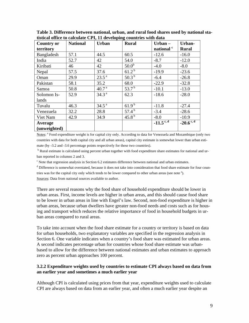
Table 3. Difference between national, urban, and rural food shares used by national sta-tistical office to calculate CPI, 11 developing countries with data Country or territory

National Urban Rural Urban – national c

Urban- Rural

Bangladesh 57.1 44.5 60.5 -12.6 -16.0 India 52.7 42 54.0 -8.7 -12.0 Kiribati 46 42 50.0b -4.0 -8.0 Nepal 57.5 37.6 61.2 b -19.9 -23.6 Oman 29.9 23.5 a 50.3 b -6.4 -26.8 Pakistan 58.1 35.2 68.0 -22.9 -32.8 Samoa 50.8 40.7 a 53.7 b -10.1 -13.0 Solomon Is-lands

52.9 34.3 a 62.3 -18.6 -28.0

Tuvalu 46.3 34.5 a 61.9 b -11.8 -27.4 Venezuela 32.2 28.8 57.4 b -3.4 -28.6 Viet Nam 42.9 34.9 45.8 b -8.0 -10.9 Average (unweighted)

-11.5 c, d -20.6 c, d

Notes: a Food expenditure weight is for capital city only. According to data for Venezuela and Mozambique (only two countries with data for both capital city and all urban areas), capital city estimate is somewhat lower than urban esti-mate (by -3.2 and -3.6 percentage points respectively for these two countries). b Rural estimate is calculated using percent urban together with food expenditure share estimates for national and ur-ban reported in columns 2 and 3. c Note that regression analysis in Section 6.2 estimates difference between national and urban estimates. d Difference is somewhat overstated, because it does not take into consideration that food share estimate for four coun-tries was for the capital city only which tends to be lower compared to other urban areas (see note a). Sources: Data from national sources available to author. There are several reasons why the food share of household expenditure should be lower in urban areas. First, income levels are higher in urban areas, and this should cause food share to be lower in urban areas in line with Engel’s law. Second, non-food expenditure is higher in urban areas, because urban dwellers have greater non-food needs and costs such as for hous-ing and transport which reduces the relative importance of food in household budgets in ur-ban areas compared to rural areas. To take into account when the food share estimate for a country or territory is based on data for urban households, two explanatory variables are specified in the regression analysis in Section 6. One variable indicates when a country’s food share was estimated for urban areas. A second indicates percentage urban for countries whose food share estimate was urban-based to allow for the difference between national estimates and urban estimates to approach zero as percent urban approaches 100 percent.

3.2.2 Expenditure weights used by countries to estimate CPI always based on data from an earlier year and sometimes a much earlier year Although CPI is calculated using prices from that year, expenditure weights used to calculate CPI are always based on data from an earlier year, and often a much earlier year despite an

9

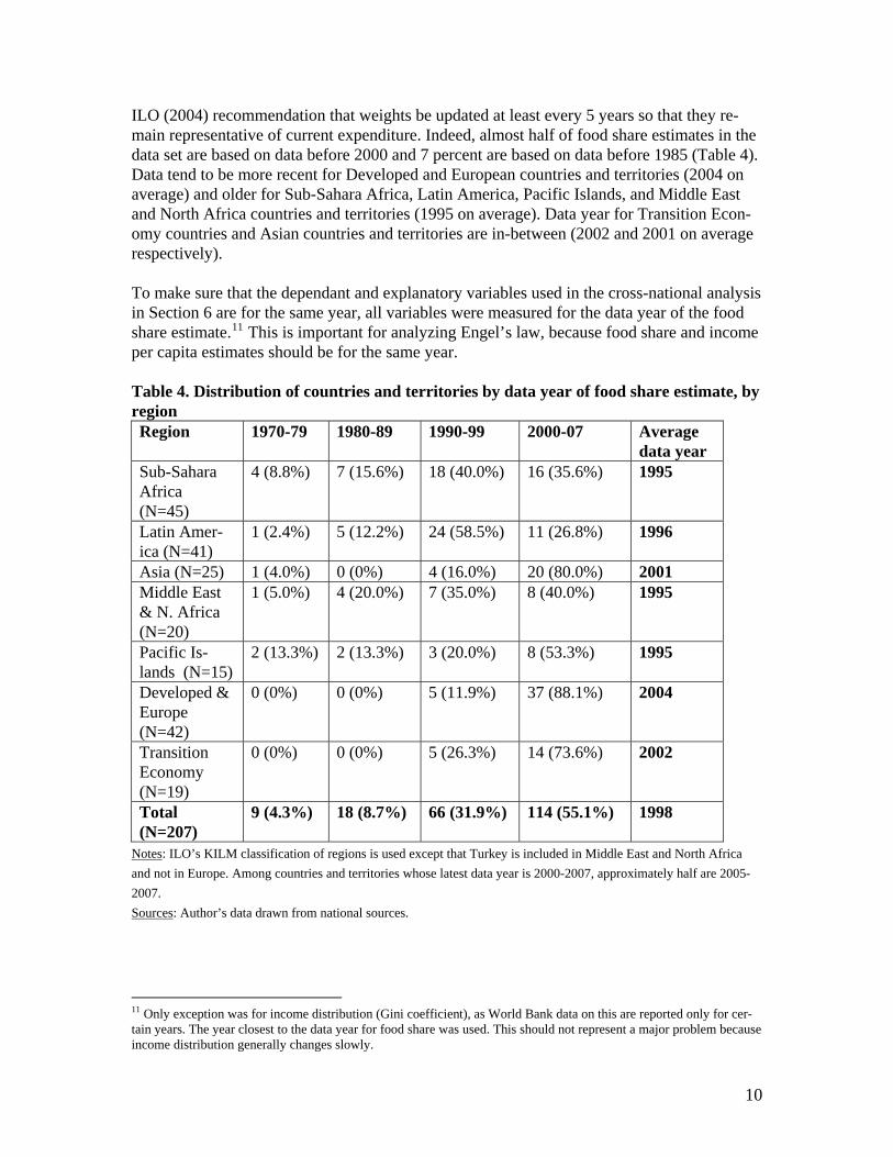
ILO (2004) recommendation that weights be updated at least every 5 years so that they re-main representative of current expenditure. Indeed, almost half of food share estimates in the data set are based on data before 2000 and 7 percent are based on data before 1985 (Table 4). Data tend to be more recent for Developed and European countries and territories (2004 on average) and older for Sub-Sahara Africa, Latin America, Pacific Islands, and Middle East and North Africa countries and territories (1995 on average). Data year for Transition Econ-omy countries and Asian countries and territories are in-between (2002 and 2001 on average respectively). To make sure that the dependant and explanatory variables used in the cross-national analysis in Section 6 are for the same year, all variables were measured for the data year of the food share estimate.11 This is important for analyzing Engel’s law, because food share and income per capita estimates should be for the same year. Table 4. Distribution of countries and territories by data year of food share estimate, by region Region 1970-79

1980-89 1990-99 2000-07 Average

data year Sub-Sahara Africa (N=45)

4 (8.8%) 7 (15.6%) 18 (40.0%) 16 (35.6%) 1995

Latin Amer-ica (N=41)

1 (2.4%) 5 (12.2%) 24 (58.5%) 11 (26.8%) 1996

Asia (N=25) 1 (4.0%) 0 (0%) 4 (16.0%) 20 (80.0%) 2001 Middle East & N. Africa (N=20)

1 (5.0%) 4 (20.0%) 7 (35.0%) 8 (40.0%) 1995

Pacific Is-lands (N=15)

2 (13.3%) 2 (13.3%) 3 (20.0%) 8 (53.3%) 1995

Developed & Europe (N=42)

0 (0%) 0 (0%) 5 (11.9%) 37 (88.1%) 2004

Transition Economy (N=19)

0 (0%) 0 (0%) 5 (26.3%) 14 (73.6%) 2002

Total (N=207)

9 (4.3%) 18 (8.7%) 66 (31.9%) 114 (55.1%) 1998

Notes: ILO’s KILM classification of regions is used except that Turkey is included in Middle East and North Africa and not in Europe. Among countries and territories whose latest data year is 2000-2007, approximately half are 2005-2007. Sources: Author’s data drawn from national sources.

11 Only exception was for income distribution (Gini coefficient), as World Bank data on this are reported only for cer-tain years. The year closest to the data year for food share was used. This should not represent a major problem because income distribution generally changes slowly.

10

3.2.3 Countries use different definitions of what is included in reported food expendi-ture Although there is wide acceptance and use of an international standard expenditure classifica-tion (COICOP: Classification of Individual Consumption according to Purpose),12 national statistical offices often differ in how they classify household expenditures. Cross-country dif-ferences are compounded by the fact that the current version of COICOP was adopted around 2000, which means that expenditure weight data before 2000 and a few years afterwards (since it takes time for many countries to adopt a new standard classification) generally used an earlier version of COICOP. By far the two most important differences between countries in how food expenditure is measured are: (i) whether alcohol and tobacco expenditure is in-cluded in food expenditure (as in previous COICOP) or as their own separate expenditure category (as in current COICOP), and (ii) whether expenditure for food taken away from home is included in food expenditure or in a separate category of restaurants and hotels (as in previous and current COICOP). 3.2.3.1 Some countries include expenditure for alcohol and tobacco in food expenditure while others do not Despite alcohol and tobacco constituting a separate expenditure category in the current COI-COP, 43 percent of the 207 countries and territories in my data set included alcohol and/or tobacco in food expenditure (Table 5).13 This ranged from about 20 percent of Pacific Island countries and territories and 25 percent of Developed and European, to about 45 percent of Sub-Sahara African, Latin American, Asian and Transition Economy countries and territo-ries, and to about 75 percent of Middle East and North African countries and territories. Among countries and territories that included alcohol and/or tobacco expenditure in food ex-penditure, approximately one-quarter included alcohol but not tobacco, and about ten percent included tobacco but not alcohol (mainly Islamic countries which ban alcohol and do not measure alcohol expenditure). To increase cross-country comparability, alcohol and tobacco expenditure was subtracted from reported food expenditure when alcohol and/or tobacco ex-penditure was included in food expenditure.14

12 COICOP (Classification of Individual Consumption according to Purpose) is a nested classification, see ILO (2004). Its current version has 12 divisions at the first level and 46 groups at the second level. First level divisions are: food and non-alcoholic beverages (comprised of 2 groups); alcoholic beverages, tobacco and narcotics (comprised of 3 groups); clothing and footwear (2 groups); housing, water electricity gas and other fuels (5 groups); furnishings, house-hold equipment and routine household maintenance (5 groups); health (3 groups); transport (3 groups); communication (3 groups); recreation and culture (6 groups); education (5 groups); restaurants and hotels (2 groups); miscellaneous goods and services (7 groups). 13 Part of the reason for such a high percentage is because alcohol and tobacco expenditure was included under food expenditure in previous COICOP. 14 When information on percentage of household expenditure for alcohol and/or tobacco for a country or territory was available for the data year, this percentage was subtracted from the reported food share of household expenditure. When information was not available for a country or territory on the percentage of household expenditure for alcohol and/or tobacco expenditure for the data year, a value from an earlier year was used when available. When a value was not available for any year for the country or territory, the trimmed mean percentage for countries and territories in the sub-region was used. Note that alcohol and tobacco expenditure accounts for around 4 percent of total household ex-penditure on average.

11

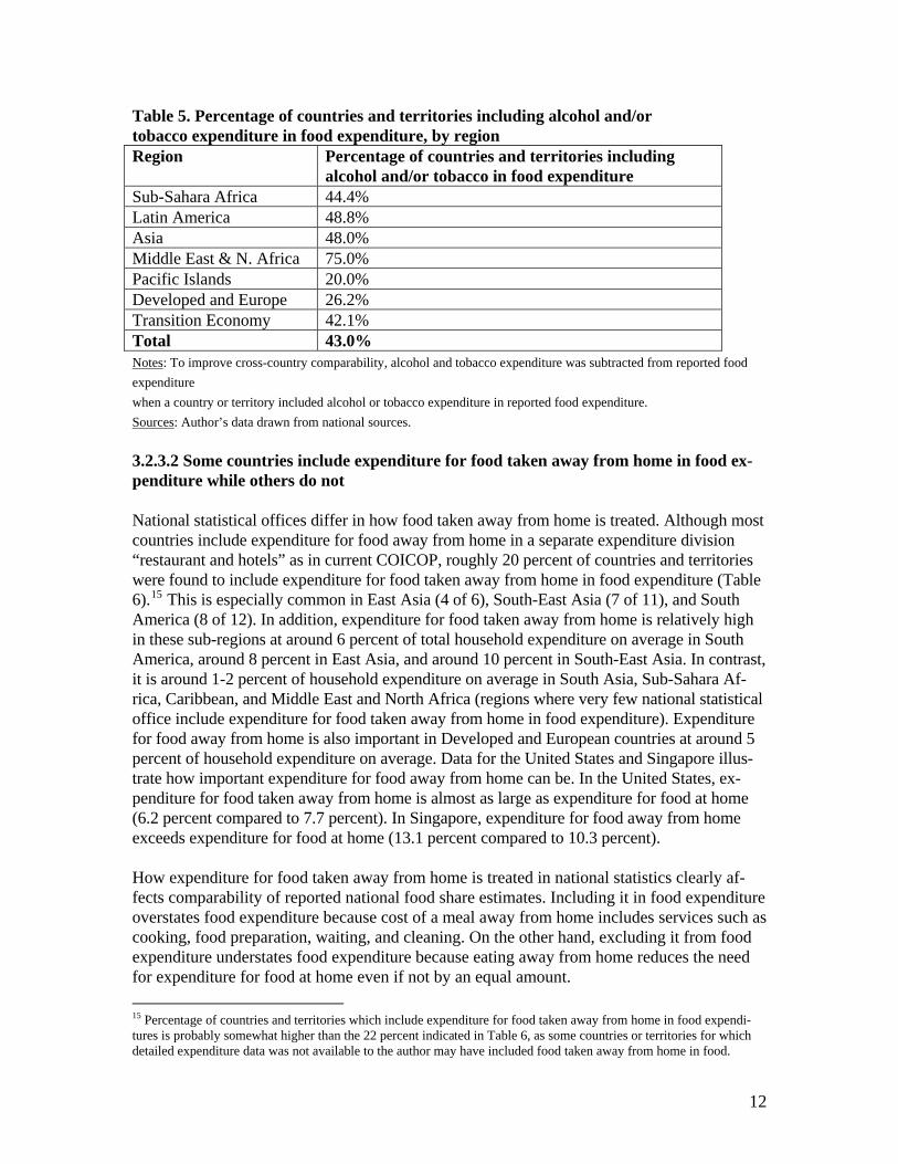
Table 5. Percentage of countries and territories including alcohol and/or tobacco expenditure in food expenditure, by region Region Percentage of countries and territories including

alcohol and/or tobacco in food expenditure Sub-Sahara Africa 44.4% Latin America 48.8% Asia 48.0% Middle East & N. Africa 75.0% Pacific Islands 20.0% Developed and Europe 26.2% Transition Economy 42.1% Total 43.0% Notes: To improve cross-country comparability, alcohol and tobacco expenditure was subtracted from reported food expenditure when a country or territory included alcohol or tobacco expenditure in reported food expenditure. Sources: Author’s data drawn from national sources. 3.2.3.2 Some countries include expenditure for food taken away from home in food ex-penditure while others do not National statistical offices differ in how food taken away from home is treated. Although most countries include expenditure for food away from home in a separate expenditure division “restaurant and hotels” as in current COICOP, roughly 20 percent of countries and territories were found to include expenditure for food taken away from home in food expenditure (Table 6).15 This is especially common in East Asia (4 of 6), South-East Asia (7 of 11), and South America (8 of 12). In addition, expenditure for food taken away from home is relatively high in these sub-regions at around 6 percent of total household expenditure on average in South America, around 8 percent in East Asia, and around 10 percent in South-East Asia. In contrast, it is around 1-2 percent of household expenditure on average in South Asia, Sub-Sahara Af-rica, Caribbean, and Middle East and North Africa (regions where very few national statistical office include expenditure for food taken away from home in food expenditure). Expenditure for food away from home is also important in Developed and European countries at around 5 percent of household expenditure on average. Data for the United States and Singapore illus-trate how important expenditure for food away from home can be. In the United States, ex-penditure for food taken away from home is almost as large as expenditure for food at home (6.2 percent compared to 7.7 percent). In Singapore, expenditure for food away from home exceeds expenditure for food at home (13.1 percent compared to 10.3 percent). How expenditure for food taken away from home is treated in national statistics clearly af-fects comparability of reported national food share estimates. Including it in food expenditure overstates food expenditure because cost of a meal away from home includes services such as cooking, food preparation, waiting, and cleaning. On the other hand, excluding it from food expenditure understates food expenditure because eating away from home reduces the need for expenditure for food at home even if not by an equal amount. 15 Percentage of countries and territories which include expenditure for food taken away from home in food expendi-tures is probably somewhat higher than the 22 percent indicated in Table 6, as some countries or territories for which detailed expenditure data was not available to the author may have included food taken away from home in food.

12

The decision on how to treat expenditures for food taken away from home is made more dif-ficult by the fact that the difference between cost of a meal away from home and a similar meal prepared at home is not only unknown but it also varies across countries, regions and development levels. Complicating matter further, is the need to have an estimate of expendi-ture for food taken away from home for each country and territory. Yet as far as the author is aware, no international database on expenditure for food taken away from home is available and even after considerable effort I found estimates for less than half the countries and terri-tories in the world. 16 This means that national values would need to be imputed for most countries and territories. Given uncertainties in how to treat expenditure for food taken away from home - - (i) un-known difference in cost of a meal taken away from home and a similar meal prepared at home; (ii) unknown expenditure for food taken away from home for most countries and terri-tories; and (iii) variability across countries in both expenditure for food taken away from home and difference in cost of a meal away from home and similar meal prepared at home - - I decided to use food expenditure excluding expenditure for food taken away from home in the empirical analysis in Section 6. This is what most countries do and what COICOP rec-ommends. However since excluding food taken away from home could affect results, a de-tailed analysis of how expenditure for food at home is affected by expenditure for food away from home is provided in Appendix A. This analysis indicates that specifying expenditure for food away from home as an explanatory variable does not have much of an effect on regres-sion results reported in Section 6. Although expenditure for food taken away from home is found to reduce expenditure for food at home as expected, the relationship is sensitive to the sample of countries and territories and is not always significant. These results may be due to the generally small value of the food included in meals away from home for most countries and therefore often only a small reduction in the need for expenditure for food at home; or to the difficulty of taking into account the strong influence that culture and history have on household expenditure for meals away from home.17

16 It is interesting to note in a diversion that ignoring the value of unpaid household work preparing meals at home has a major effect on both observed differences in the food share of household expenditure across countries at one point in time as well as on observed changes in countries in food share over time. As countries develop and people increasingly work away from home, households spend less time preparing food (e.g. grinding spices and canning and preserving food become uncommon) and increasingly purchase prepared and processed food (e.g. canned and frozen food become common as eventually do TV dinners and deli counters in supermarkets). These increase food costs and therefore food share of household expenditure compared to what it would have been if the time to prepare meals at home remained the same over time. This in turn causes GDP per capita to increase faster than if meal preparation at home remained changed, and consequently to indicate that material well-being increased more rapidly than it actually did. This prob-lem is similar, but of much greater importance, to the often noted example in economics of how marrying one’s house-keeper or nanny decreases GDP. 17 Using reasonable assumptions for the level of expenditure for food taken away from home (see Table 6) and differ-ence in cost of a meal away from home and a similar meal prepared at home (50 percent in developing countries and 75 percent in Developed and European countries, see Appendix A), food share would increase only by about 1 percentage point in a typical Developed or European country and in a typical developing country outside of East Asia, South-East Asia, South America and Central America if expenditure for food taken away from home was included in food expen-diture. The increase in food share using these assumptions, however, would be sizable in East Asia and South-East Asia (around 5 percentage points) as well as in South America and Central America (around 3 percentage points).

13

Table 6. Percentage of countries and territories including expenditure for food taken away from home in food expenditure and average percentage of household expenditure for food taken away from home when included, by region Region Percent of countries and

territories including food taken away from home in food expenditure

(When included) Average (median) percentage of household expenditure

Sub-Sahara Africa 8.8% 1.0 Latin America 29.3%* 6.1 Asia 50.0%* 9.0 Middle East & N. Africa 15.0% 0.9 Pacific Islands 33.3% 1.1 Developed and Europe 21.4%* 5.3 Transition Economy 5.2% 2.0 Total 22.2% 5.3 Notes: * Especially common to include expenditure for food taken away from home in food expenditure in following sub-regions: South-East Asia (7 of 11 countries and territories), East Asia (4 of 6), and South America (8 of 12). See Appendix A for further statistics on expenditure for food taken away from home. Sources: Author’s data drawn from national sources. 3.2.4 Countries differ in extent to which government provides free or subsidized goods and services Provision by government of free or subsidized non-food goods and services affects the food share of household expenditure, because it reduces the need for expenditure on these goods and services. This necessarily increases the percentage of total expenditures households for food. When a country has free universal health care, medical expenditure of households are reduced and therefore the food share of household expenditure is increased. When a country subsidizes transportation or housing, expenditure on these by households are reduced and therefore the food share of household expenditure is increased. Provision of free or low cost goods and services by the state is especially important in Transition Economy countries where change has been slow in this regard (Herrmann and Polgar, 2007). Because data are not available for many countries on government subsidies, a binary variable is used in the regression analysis in Section 6 to identify Transition Economy countries. A priori expecta-tion is that the food share of household expenditure will be higher in Transition Economy countries ceteris paribus.18 3.2.5 Some countries impute a value to owner occupied housing while others do not National statistical offices differ in how they treat owner occupied housing when estimating household expenditure weights. Many countries impute a value to owner occupied housing

18 It is worth noting that Transition Economy countries are less likely than other countries to impute a value to owner occupied housing, and that this increases the observed food share of household expenditure for Transition Economy countries (see Section 3.2.5). On the other hand, Transition Economy countries have lower per unit food costs com-pared to other countries which should reduce food share. For example according to ILO data on retail food prices (www.laborsta.ilo.org), the per kg price of white wheat flour (a food item with similar quality in all countries) was 30 percent lower on average in 2005 in Transition Economy countries than in the United States.

14

while many others do not. 19, 20 Even European countries, which harmonize national statistics, are unable to agree on whether or not to impute a value to owner occupied housing. Eleven impute a value, and sixteen do not impute a value (Herrmann and Polgar, 2007). Imputing a value to owner occupied housing increases measured total household expenditure (denominator used to calculate food share), and therefore lowers reported food share of household expenditure. 21 Differences across countries in this regard should be especially im-portant in explaining differences in the food share of household expenditures among high income countries where food shares are low and housing costs are high. Since it was not pos-sible to ascertain for most countries when a value was imputed to owner occupied housing or how large it was, this aspect of cross-country comparability is not controlled for in the cross-national analysis in Section 6. 3.3 Income per capita in PPP and other explanatory variables Income per capita (GDP per capita in PPP) and household income distribution (Gini coeffi-cient) data were drawn from the World Development Indicators database of the World Bank (2008) except that GDP per capita in PPP was taken from online Fact Sheets (CIA, 2008) for 26 countries or territories not available from the World Bank. Almost all of these additional countries or territories are very small, with less than one-half million people in 2005. 22, 23 Data on percent of population less than age 15 were taken from a United Nations online data-base (UN Statistical Division, 2008). Region of countries and territories and list of Transition Economy countries were from ILO (ILO KILM, 2007). List of small island developing states was from United Nations (UN OHRLLS, 2008).

Explanatory variables were measured for the same year as the data year of the food share of household expenditure.24 World Bank (2008) provides estimates on its web site of GDP per capita in 2005 PPP for 1980-2007 based on its 2007 and 2008 revisions and improved meth-odology. For the 26 countries or territories whose value was drawn from a CIA Fact Sheet, GDP per capita in PPP estimates were adjusted so that they were for the same year as the food share data using information from the World Bank on change in real per capita income between GDP per capita in PPP data year and food share data year.

19 There are three main approaches used to estimate an imputed value to owner occupied housing: actual outlays of households; acquisition costs; and value of the flow of shelter services such as indicated by market rent for equivalent housing (Turvey, 1979; ILO, 2004). The alternative of not imputing a value to owner occupied housing implicitly as-sumes a zero value. 20 Total value of owner occupied housing in a country depends on extensiveness of home ownership and value per house. 21 Housing is always one of the largest expenses for households. In high income countries, housing is usually the most important expense among the 12 main expenditure divisions in COICOP. In lower income countries, housing is usually the second most important expense of households (food is usually first). 22 14 had less than 50,000 persons; 4 had 50,000-99,000 persons; 4 had 100,000 to 249,000 persons; and 1 had 250,000-499,000 persons. The three remaining countries or territories were either new (Kosovo) or ignored by the World Bank for political reasons (Taiwan and Puerto Rico). 23 GDP per capita in PPP for four French overseas departments were estimated by multiplying a recent estimate of the ratio between their GDP per capita in PPP to France’s GDP per capita in PPP according to INSEE by the change in real GDP per capita in France between the year for this ratio and the food share data year. 24 Only exception is for Gini coefficient, because the World Bank provides Gini estimates only for certain years. This is not expected to represent a major problem, because income distribution changes slowly over time.

15

3.4 National income per capita in PPP: Aspects of reduced comparability across countries Two aspects of how national income per capita in PPP (explanatory variable used to measure material standard of living in the cross-national analysis) is measured that affect cross-country comparability are discussed below - - imprecision and possible biases; and relevance of GDP per capita in PPP as a measure of material standard of living of households. 3.4.1 PPP is difficult to measure and this imprecision could cause estimated GDP per capita in PPP to be biased To investigate Engel’s law across countries, it is necessary to have internationally compara-ble estimates of national material living standard. This requires internationally comparable estimates of the purchasing power of national currencies. Purchasing power parities (PPP) estimated by the World Bank are recognized as the best measure of differences across coun-tries in the purchasing power of national currencies and therefore are used in this paper. Unfortunately, PPP estimates and therefore estimates of GDP per capita in PPP are fraught with imprecision and possible biases, especially for countries at different levels of economic development and in different regions. This problem is illustrated by the size and pattern of the recent 2007 and 2008 World Bank revisions of GDP per capita in PPP (African Devel-opment Bank, 2007 for Africa; Asian Development Bank, 2007 for Asia; ECLAC 2008 for South America; and World Bank, 2008 for global results). China’s GDP per capita in PPP, for example, is about 40 percent lower according to the World Bank’s recently revised esti-mate compared to the World Bank’s previous estimate. India’s GDP per capita is about 35 percent lower. Indeed, there are systematic differences in new World Bank estimates com-pared to previous estimates other than for Developed and European and Transition Economy countries and territories (Table 7). New GDP per capita in PPP estimates are substantially lower on average compared to previous estimates in Sub-Saharan Africa (by 11 percent), Asia (by 20 percent), and Pacific Islands (by 27 percent). At the same time, they are substan-tially higher on average in Middle East and North Africa (by 19 percent), and somewhat higher on average in Latin America (by 7 percent). Upward revisions are especially large for oil-rich exporting countries; average ratio of new World Bank estimates to previous World Bank estimates for oil-rich exporting countries is 1.36 for eight Middle East or North African countries, 1.51 for two South American countries, and 1.88 for five Sub-Saharan African countries. Revised estimates are basically unchanged on average for Developed and Euro-pean countries and Transition Economy countries as well as for most of South and Central America.

16

Table 7. Ratio of recently revised World Bank estimate of GDP per capita in PPP to previous World Bank estimate, by region Region Average of na-

tional ratios (unweighted)

Comment

Sub-Saharan Africa (N=40)

0.89 Average is 0.75 when five oil-rich coun-tries (with 1.87 average) are excluded.

Asia (N=20) 0.80 Average is 0.73 when four high income Asian countries or territories (with 1.10 average) are excluded.

Latin America (N=28) 1.07 Average is higher in Caribbean at 1.16 and in two oil-rich countries at 1.51. Av-erage in other countries or territories is 0.96.

Pacific Islands (N=6) 0.73 Middle East and N. Af-rica (N=17)

1.19 Average is 0.86 for four North African countries, and 1.36 for eight Middle East oil exporters.

Transition Economy (N=16)

1.00

Developed and Europe (N=33)

1.00

Notes: Calculated ratio for each country was adjusted by the value of this ratio for the comparator country, the United States (1.122), because previous estimates were expressed in 2000 PPPs and recently revised estimates were expressed in 2005 PPPs. Sources: World Bank World Indicators databases. One reason why it is difficult to measure PPP is that while a set of expenditure weights is re-quired to calculate PPP, any particular set cannot be appropriate for all countries and all pur-poses, especially for dissimilar countries. This is especially a problem for countries at different development levels and in different regions. For example, households in Viet Nam spend a substantial percent of total expenditure on rice and very little on automobiles. In the United States in contrast, households spend very little on rice but a substantial percent on automobiles. So, if the basket of goods and services used to estimate PPP assigned a high weight to rice, it would reflect what is important for households in Viet Nam but not for households in the United States. In contrast if automobiles were assigned a high weight, this would be relevant for the United States but not for Vietnam. Because of this problem, the In-ternational Comparability Program (ICP) began by estimating PPPs between countries in country groupings/regions. Considerable effort for one or two countries from each country group/region was then put into estimating PPPs between them so that groups/regions could be linked (World Bank, 2008a). The use of similar link values between groups/regions for all countries within each group/region helps explain why there are similar differences for coun-tries within a region and development level between revised and previous estimates of GDP per capita in PPP. Despite problems with estimating PPP, and therefore GDP per capita in PPP, they remain the best available measure of real national per capita income across countries, and for this reason

17

are used in this paper. At the same time, it is necessary to be cognizant that the material stan-dard of living of a particular country or region could be poorly measured by GDP per capita in PPP, and so could help explain why a particular country has a large residual in the cross-national regression analysis in Section 6. 3.4.2 GDP per capita in PPP does not accurately measure material standard of living under certain circumstances

GDP per capita does not always accurately measure material standard of living of households in a country. It overestimates standard of living when a large number of workers who con-tribute to GDP are not counted as part of a country’s population when GDP per capita is cal-culated. This can occur when a large number of day workers cross-over the border to sleep each evening (e.g. Luxembourg), when there are many undocumented immigrant workers (many countries), and when documented foreign workers are not counted in a country’s population when per capita GDP is calculated. GDP per capita also overstates standard of living of households when countries with large commodity exports such as oil (e.g. Saudi Arabia, and Gabon) or when a small country or territory has a large financial services sector which substantially boosts GDP but only partially increases household incomes (e.g. Jersey and Bermuda). GDP per capita in PPP understates household income in small states (usually territories) which receive large transfers relative to GDP from another government (e.g. St. Helena, American Samoa, Wallis and Fortuna, St Pierre and Miquelon). This information is useful for explaining residuals in regression analysis. Since GDP per capita in countries or territories with an especially high GDP per capita in PPP often overestimates material standard of living of households, GDP per capita in PPP is capped in the cross-national analysis in Section 6 at approximately the highest value ob-served for a reasonable size country (Norway). Capping GDP per capita has the added advan-tage of reducing the effect on regression results of a few atypical countries and territories with exceptionally high per capita income in PPP. 25

4. Analytical framework

Since the main purpose of this paper is to analyze the extent to which Engel’s law operates across countries in the 21st century, the dependant variable is food share of household expen-diture and the main explanatory variable is income per capita in PPP. The expected relation-ship between food share of household expenditure and income per capita in PPP is discussion in Section 4.1. Section 4.2 discusses behavioral factors other than per capita income that might affect the observed food share of household expenditure in a country. Section 4.3 dis-cusses the functional form used in the regression analysis in Section 6. 4.1 Relationship between food share of household expenditure and income per capita in PPP Food share of household expenditure is expected to be negatively related to income per capita in PPP in keeping with Engel’s law, which implies that the income elasticity of food expendi- 25 This only affects five very small countries or territories: San Marino, Jersey, Qatar, Luxembourg and Bermuda.

18

ture falls as per capita income increases. In keeping with earlier studies, the income elasticity of food expenditure is expected to fall from below 1.0 at low per capita income levels where need for increased calories are relatively great, to somewhere around 0.6 at middle per capita income levels, and to around 0.2 at high per capita income levels (e.g. Houthakker, 1957; Seale and Regmi, 2006). Although food expenditure is expected to increase with per capita income largely because more expensive foods replace lower cost foods (e.g. more expensive varieties of rice such as long grained rice increasingly replace less expensive varieties of rice such as short grained rice; 26 relatively expensive animal-based products such as meat, fish, milk and egg are increasingly introduced into diets; and better cuts of meat increasingly re-place worse cuts of meat, see Anker, 2005), food share falls with per capita income because non-food needs, costs and expenditures increase rapidly along with development and urbani-zation such as for transportation, housing, medical care, recreation, and communication. 4.2 Factors other than per capita income possibly related to food share of household ex-penditure Three substantive factors expected to affect the observed food share of household expendi-ture in a country are discussed in this section. Household income inequality in a country should negatively affect average food share of household expenditure, because of how expenditure weights are calculated where every dol-lar spent counts equally. This means that high income households are especially important in determining expenditure weights, and therefore that average food share is affected by the dis-tribution of household income since higher income households have low food shares and low income households have high food shares. South African data (Statistics South Africa, 2002) demonstrate how much food share of household expenditure varies by household income.27 Whereas “very low income” and “low income” households in South Africa together are re-sponsible for 4 percent of total household expenditure and have a food expenditure share of 47 percent, “very high income” households in South Africa are responsible for 71 percent of total household expenditure and have a food expenditure share of only 14 percent.28 Regres-sion analysis in Section 6 includes Gini coefficient of household income from the World Bank to measure household income distribution. It is expected to have a negative sign. Average household size should affect allocation of household expenditure between food and non-food expenditure, because economies of scale differ for food and non-food expenditure. 29 Average household size is expected to be positively related to food share of household ex-

26 According to recent fieldwork by the author in India, Bangladesh, China and Vietnam, lower quality rice tends to be around one-third less expensive than higher quality rice (Anker, 2005 for India and Bangladesh; unpublished reports for China and Vietnam). 27 Household expenditure shares are always estimated using plutonic weighting where each dollar spent is weighted equally. While it is possible to use democratic weighting where each household is weighted equally, this is never done (although UK excludes expenditures by top 4 percent of households in terms of income). See Turvey (1989) and ILO (2004) for detailed discussions on approaches to weighting. 28 This terminology regarding income classes is used in the source. “Middle income” and “high income” households in South Africa are responsible for 8 and 17 percent respectively of total household expenditure and have food shares of 40 and 30 percent respectively. 29 Although household size is typically included in empirical analyses of household expenditure within countries using household data, cross-national analyses of food expenditure generally do not include household size as an explanatory variable (see for example Seale and Regmi, 2006).

19

penditure ceteris paribus, because household economies of scale are greater for non-food ex-penditure (such as for housing) than for food expenditure. United Nations’ data on percent children in the population (below age 15 years) are used in the regression analysis to proxy for average household size, because data on average household size are not available for many countries, especially historical data.30 Relative prices of food and non-food items should affect the allocation of household expendi-ture between food and non-food. Studies investigating the relationship between food expendi-ture shares and national income often control for prices. Seale and Regmi (2006) found that the price elasticity of food, beverages and tobacco (one of their expenditure groups) was sig-nificant with an elasticity of approximately 0.6 for low income countries, 0.5 for middle in-come countries, and 0.1 to 0.3 for high income countries.31 Although analysis in Section 6 does not explicitly consider price differences across countries because these data were not available to the author for many countries, an explanatory variable identifying island states is specified in the regression analysis because food prices are relatively high in these states. For example according to 2005 data on food prices for 75 countries and territories (www.laborsta.ilo.org), the per kg price of white wheat flour (a food which is similar in qual-ity in all countries) was 61 percent higher on average in island states than in the United States, 22 percent higher than in Developed and European countries and territories, and 63 percent higher than other developing countries. 4.3 Functional form of relationship between food share of household expenditure and national income per capita in PPP Food share of household expenditure is the dependant variable in the empirical analysis in Section 6, because it is the appropriate variable for investigating Engel’s law. Previous stud-ies of household expenditure, on the other hand, have generally used food expenditure as the dependant variable, because many researchers are interested in the income elasticity of food expenditure. This implies that regression coefficients estimated in Section 6 have to be con-verted into income elasticities to arrive at comparable values to those in most previous stud-ies. Another implication is that regression fits (measured by R2) should be lower when food expenditure is the dependant variable, since the absolute value of food expenditure almost has to increase with income per capita whereas the share of food expenditure does not have to decrease with income per capita. There is no agreement in the research literature on the appropriate functional form to estimate the relationship between food expenditure and total household expenditure. In the 1950s, the double log function, which assumes a constant income elasticity of food expenditure, was popular (e.g. Prais and Houthakker 1955 for British households; and Houthakker 1957 for approximately 30 countries). Other non-linear models are now generally used to allow the income elasticity of food expenditure to fall as income increases such as log linear, quadratic, quadratic log, AIDS, and Slutsky functions (Seale and Regmi, 2006). Since there is no agreement on the best functional form to use especially when the dependant variable is food 30 Although percentage children in the population is an imperfect proxy for average household size since it does not consider how common are nuclear and extended families, percent children should be positively and strongly related to average household size. 31 Studies of household expenditure across households within countries in contrast generally do not consider price dif-ferences on the assumption that all households in a country face the same prices.

20

share, the present study uses linear, quadratic, log and quadratic log functions in the regres-sion analysis to observe which provides the best fit. Regressions are also re-estimated for dif-ferent development levels to observe the robustness of the relationship between the food share of household expenditure and income per capita in PPP and to observe whether this relationship differs by development level. It is important to point out that when the dependant variable is food share the income elastic-ity of food expenditure is non-linear even when a linear function is used. To illustrate this, say that the food share of expenditure is a linear function of total expenditure where F indi-cates food expenditure, E indicates total household expenditure, and a and b are estimated coefficients:

F/E = a + bE

Therefore, food expenditure is a quadratic function of total expenditure, and the income elas-ticity of food expenditure is a quadratic function of total expenditure:

F = aE + bE2, with

Income elasticity of F = (aE+2bE2)/F = 1 + bE2/predicted F

Since log of income per capita in PPP provides the best fit in the regression analysis in Sec-tion 6 (and is in any case often used in cross-national studies), this implies that the income elasticity of food expenditure is as follows: F/E = a + bLnE, with

Income elasticity of F = 1+b/Predicted F/E

5.0 Reconfirming Engel’s law across households within countries

Since previous studies of food expenditure and Engel’s law have been based mostly on analysis of household expenditure data within countries, and mostly for high income coun-tries, it is worth investigating whether Engel’s law operates in the 21st century at the house-hold level within countries at different development levels before moving onto a cross-national analysis in Section 6. A recent study for Ethiopia for example (Kedir and Girma, 2007) raised doubt about Engel’s law at very low household income levels as it found that food share of household expenditure increased in Addis Ababa, Ethiopia with increases in household expenditure up to around median expenditure.32

With this in mind, I looked at household income and expenditure survey data available on an ILO website (www.laborsta.ilo.org) that are tabulated by income class from 46 countries or territories (Table 8). In keeping with Engel’s law, percent food fell with household income in all countries or territories. When expenditure shares of adjacent expenditure classes were compared (i.e. expenditure class 2 compared to expenditure class 1, expenditure class 3 com-

32 Kedir and Girma (2007) also cite a study for rural Pakistan (Bhalotra and Attfield, 1998) which found that food share increased at low household income levels.

21

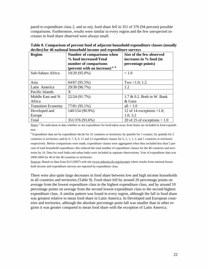
pared to expenditure class 2, and so on), food share fell in 351 of 376 (94 percent) possible comparisons. Furthermore, results were similar in every region and the few unexpected in-creases in food share observed were always small. Table 8. Comparison of percent food of adjacent household expenditure classes (usually deciles) for 46 national household income and expenditure surveys Region Number of comparisons when

% food increased/Total number of comparisons (percent with an increase) a, b

Size of the few observed increases in % food (in percentage points)

Sub-Sahara Africa 19/20 (95.0%)

< 1.0

Asia 64/67 (95.5%) Two <1.0; 1.2 Latin America 29/30 (96.7%) 1.2 Pacific Islands X Middle East and N. Africa

22/24 (91.7%) 1.7 & 0.2. Both in W. Bank & Gaza

Transition Economy 77/81 (95.1%) all < 1.0 Developed and Europe

140/154 (90.9%) 12 of 14 exceptions <1.0; 1.0; 3.2

Total 351/376 (93.6%) 20 of 25 of exceptions < 1.0 Notes: a No indication in data whether or not expenditure for food taken away from home are included in food expendi-ture. b Expenditure data are by expenditure decile for 31 countries or territories; by quartile for 1 country; by quintile for 2 countries or territories; and by 6, 7, 8, 9, 11 and 12 expenditure classes for 5, 2, 1, 1, 2, and 1 countries or territories respectively. Before comparisons were made, expenditure classes were aggregated when they included less than 5 per-cent of total household expenditure; this reduced the total number of expenditure classes for the 46 countries and terri-tories by 10. Data for rural India and urban India were included as separate observations. Year of expenditure data was 2000-2004 for 40 of the 46 countries or territories. Sources: Based on data from ILO (2007) web site (www.laborsta.ilo.org/income) where results from national house-hold income and expenditure surveys are reported by expenditure class. There were also quite large decreases in food share between low and high income households in all countries and territories (Table 9). Food share fell by around 20 percentage points on average from the lowest expenditure class to the highest expenditure class, and by around 10 percentage points on average from the second lowest expenditure class to the second highest expenditure class. A similar pattern was found in every region, although the fall in food share was greatest relative to mean food share in Latin America. In Developed and European coun-tries and territories, although the absolute percentage point fall was smaller than in other re-gions it was greater compared to mean food share with the exception of Latin America.

22

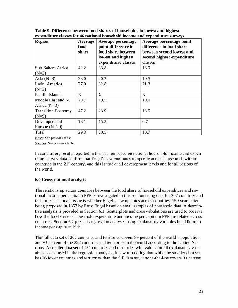
Table 9. Difference between food shares of households in lowest and highest expenditure classes for 46 national household income and expenditure surveys Region Average

food share

Average percentage point difference in food share between lowest and highest expenditure classes

Average percentage point difference in food share between second lowest and second highest expenditure classes

Sub-Sahara Africa (N=3)

42.2 33.8 16.9

Asia (N=8) 33.0 20.2 10.5 Latin America (N=3)

27.0 32.8 21.3

Pacific Islands X X X Middle East and N. Africa (N=3)

29.7 19.5 10.0

Transition Economy (N=9)

47.2 23.9 13.5

Developed and Europe (N=20)

18.1 15.3 6.7

Total 29.3 20.5 10.7 Notes: See previous table. Sources: See previous table. In conclusion, results reported in this section based on national household income and expen-diture survey data confirm that Engel’s law continues to operate across households within countries in the 21st century, and this is true at all development levels and for all regions of the world. 6.0 Cross-national analysis The relationship across countries between the food share of household expenditure and na-tional income per capita in PPP is investigated in this section using data for 207 countries and territories. The main issue is whether Engel’s law operates across countries, 150 years after being proposed in 1857 by Ernst Engel based on small samples of household data. A descrip-tive analysis is provided in Section 6.1. Scatterplots and cross-tabulations are used to observe how the food share of household expenditure and income per capita in PPP are related across countries. Section 6.2 presents regression analyses using explanatory variables in addition to income per capita in PPP. The full data set of 207 countries and territories covers 99 percent of the world’s population and 93 percent of the 222 countries and territories in the world according to the United Na-tions. A smaller data set of 131 countries and territories with values for all explanatory vari-ables is also used in the regression analysis. It is worth noting that while the smaller data set has 76 fewer countries and territories than the full data set, it none-the-less covers 93 percent

23

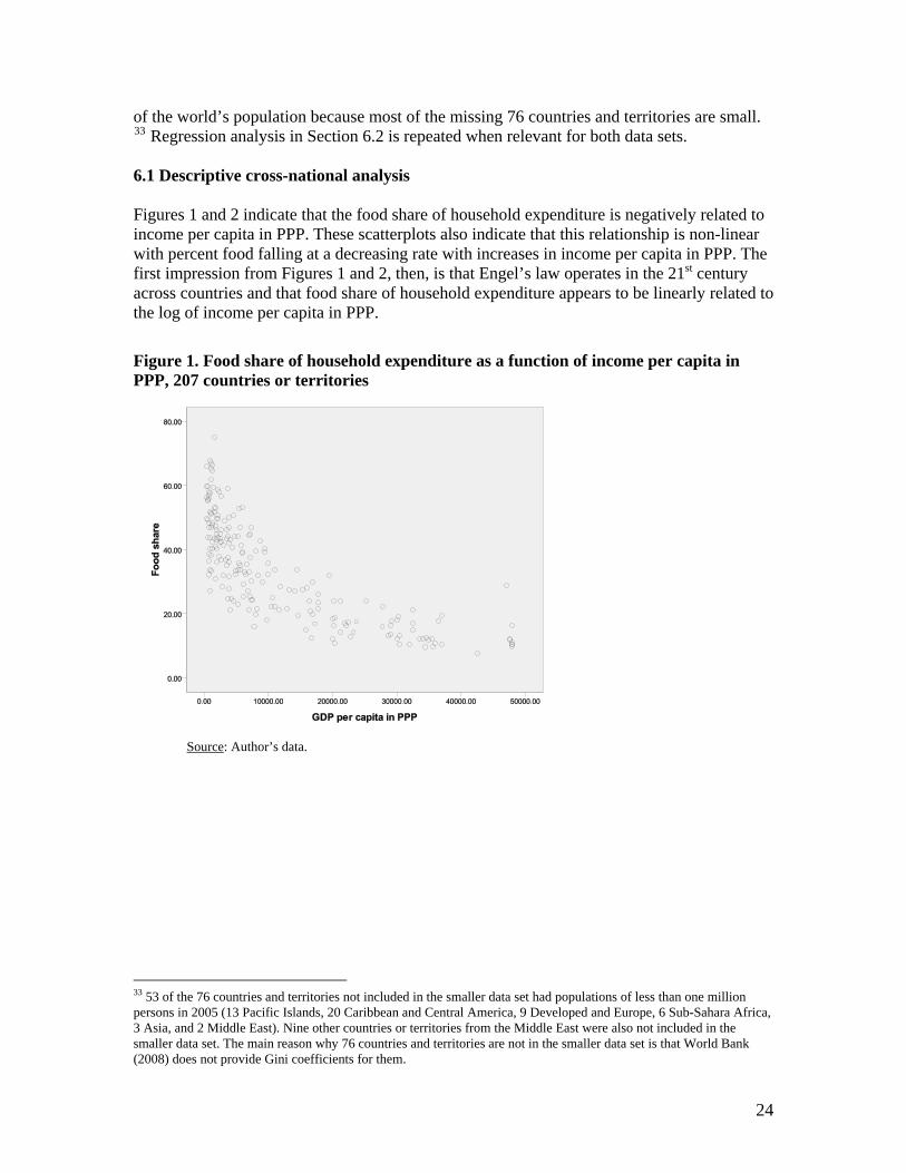
of the world’s population because most of the missing 76 countries and territories are small. 33 Regression analysis in Section 6.2 is repeated when relevant for both data sets. 6.1 Descriptive cross-national analysis Figures 1 and 2 indicate that the food share of household expenditure is negatively related to income per capita in PPP. These scatterplots also indicate that this relationship is non-linear with percent food falling at a decreasing rate with increases in income per capita in PPP. The first impression from Figures 1 and 2, then, is that Engel’s law operates in the 21st century across countries and that food share of household expenditure appears to be linearly related to the log of income per capita in PPP.

Figure 1. Food share of household expenditure as a function of income per capita in PPP, 207 countries or territories

Source: Author’s data.

33 53 of the 76 countries and territories not included in the smaller data set had populations of less than one million persons in 2005 (13 Pacific Islands, 20 Caribbean and Central America, 9 Developed and Europe, 6 Sub-Sahara Africa, 3 Asia, and 2 Middle East). Nine other countries or territories from the Middle East were also not included in the smaller data set. The main reason why 76 countries and territories are not in the smaller data set is that World Bank (2008) does not provide Gini coefficients for them.

24

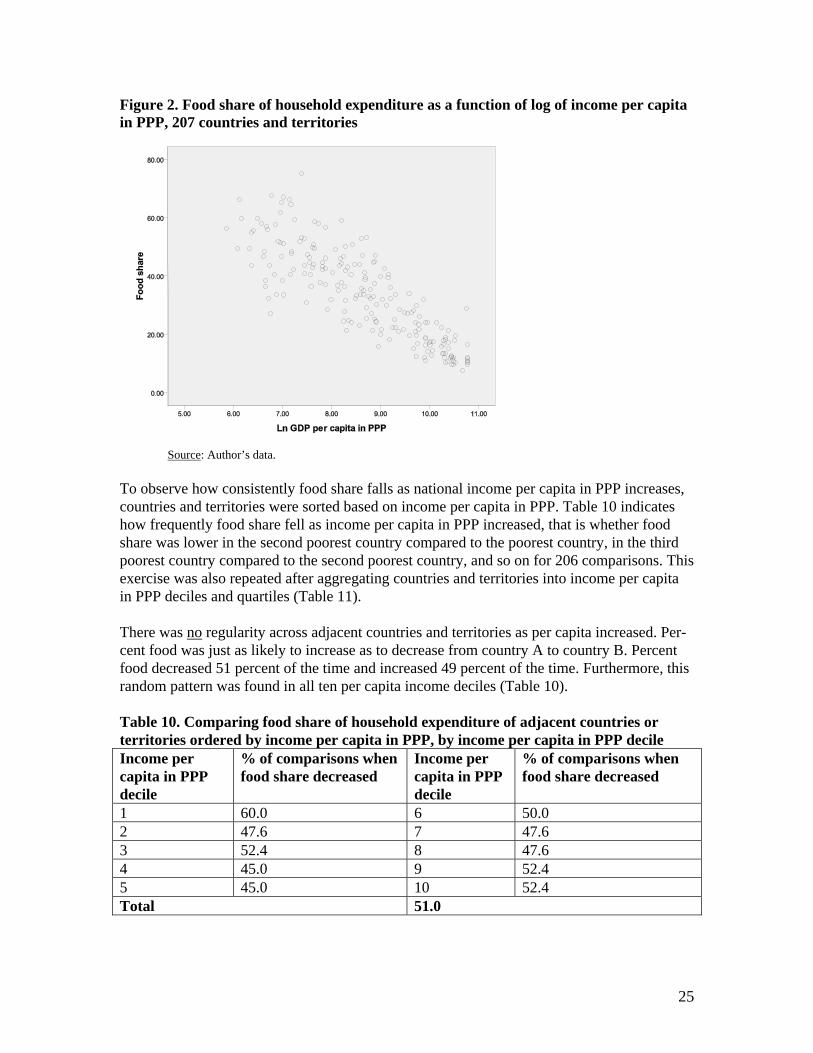
Figure 2. Food share of household expenditure as a function of log of income per capita in PPP, 207 countries and territories

Source: Author’s data.

To observe how consistently food share falls as national income per capita in PPP increases, countries and territories were sorted based on income per capita in PPP. Table 10 indicates how frequently food share fell as income per capita in PPP increased, that is whether food share was lower in the second poorest country compared to the poorest country, in the third poorest country compared to the second poorest country, and so on for 206 comparisons. This exercise was also repeated after aggregating countries and territories into income per capita in PPP deciles and quartiles (Table 11). There was no regularity across adjacent countries and territories as per capita increased. Per-cent food was just as likely to increase as to decrease from country A to country B. Percent food decreased 51 percent of the time and increased 49 percent of the time. Furthermore, this random pattern was found in all ten per capita income deciles (Table 10). Table 10. Comparing food share of household expenditure of adjacent countries or territories ordered by income per capita in PPP, by income per capita in PPP decile Income per capita in PPP decile

% of comparisons when food share decreased

Income per capita in PPP decile

% of comparisons when food share decreased

1 60.0 6 50.0 2 47.6 7 47.6 3 52.4 8 47.6 4 45.0 9 52.4 5 45.0 10 52.4 Total 51.0

25

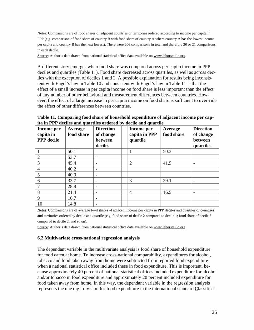
Notes: Comparisons are of food shares of adjacent countries or territories ordered according to income per capita in PPP (e.g. comparison of food share of country B with food share of country A where country A has the lowest income per capita and country B has the next lowest). There were 206 comparisons in total and therefore 20 or 21 comparisons in each decile. Source: Author’s data drawn from national statistical office data available on www.laborsta.ilo.org. A different story emerges when food share was compared across per capita income in PPP deciles and quartiles (Table 11). Food share decreased across quartiles, as well as across dec-iles with the exception of deciles 1 and 2. A possible explanation for results being inconsis-tent with Engel’s law in Table 10 and consistent with Engel’s law in Table 11 is that the effect of a small increase in per capita income on food share is less important than the effect of any number of other behavioral and measurement differences between countries. How-ever, the effect of a large increase in per capita income on food share is sufficient to over-ride the effect of other differences between countries. Table 11. Comparing food share of household expenditure of adjacent income per cap-ita in PPP deciles and quartiles ordered by decile and quartile Income per capita in PPP decile

Average food share

Direction of change between deciles

Income per capita in PPP quartile

Average food share

Direction of change between quartiles

1 50.1 1 50.3 2 53.7 + 3 45.4 - 2 41.5 - 4 40.2 - 5 40.0 - 6 33.7 - 3 29.1 - 7 28.8 - 8 21.4 - 4 16.5 - 9 16.7 - 10 14.8 - Notes: Comparisons are of average food shares of adjacent income per capita in PPP deciles and quartiles of countries and territories ordered by decile and quartile (e.g. food share of decile 2 compared to decile 1; food share of decile 3 compared to decile 2; and so on). Source: Author’s data drawn from national statistical office data available on www.laborsta.ilo.org. 6.2 Multivariate cross-national regression analysis The dependant variable in the multivariate analysis is food share of household expenditure for food eaten at home. To increase cross-national comparability, expenditures for alcohol, tobacco and food taken away from home were subtracted from reported food expenditure when a national statistical office included these in food expenditure. This is important, be-cause approximately 40 percent of national statistical offices included expenditure for alcohol and/or tobacco in food expenditure and approximately 20 percent included expenditure for food taken away from home. In this way, the dependant variable in the regression analysis represents the one digit division for food expenditure in the international standard Classifica-

26

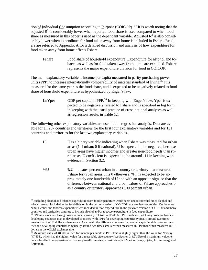
tion of Individual Consumption according to Purpose (COICOP). 34 It is worth noting that the adjusted R2 is considerably lower when reported food share is used compared to when food share as measured in this paper is used as the dependant variable. Adjusted R2 is also consid-erably lower when expenditure for food taken away from home is included in Fshare. Read-ers are referred to Appendix A for a detailed discussion and analysis of how expenditure for food taken away from home affects Fshare.

Fshare Food share of household expenditure. Expenditure for alcohol and to-bacco as well as for food taken away from home are excluded. Fshare represents the major expenditure division for food in COICOP.

The main explanatory variable is income per capita measured in parity purchasing power units (PPP) to increase internationally comparability of material standard of living.35 It is measured for the same year as the food share, and is expected to be negatively related to food share of household expenditure as hypothesized by Engel’s law.

LnYper GDP per capita in PPP.36 In keeping with Engel’s law, Yper is ex-pected to be negatively related to Fshare and is specified in log form in keeping with the usual practice of cross-national analyses as well as regression results in Table 12.

The following other explanatory variables are used in the regression analysis. Data are avail-able for all 207 countries and territories for the first four explanatory variables and for 131 countries and territories for the last two explanatory variables.

U U is a binary variable indicating when Fshare was measured for urban areas (1 if urban; 0 if national). U is expected to be negative, because urban areas have higher incomes and greater non-food needs than ru-ral areas. U coefficient is expected to be around -11 in keeping with evidence in Section 3.2.

%U %U indicates percent urban in a country or territory that measured

Fshare for urban areas. It is 0 otherwise. %U is expected to be ap-proximately one hundredth of U and with an opposite sign, so that the difference between national and urban values of Fshare approaches 0 as a country or territory approaches 100 percent urban.

34 Excluding alcohol and tobacco expenditure from food expenditure would seem uncontroversial since alcohol and tobacco are not included in the food division in the current version of COICOP, nor are they necessities. On the other hand, alcohol and tobacco expenditure was included in food expenditure in the previous version of COICOP and many countries and territories continue to include alcohol and/or tobacco expenditure in food expenditure. 35 PPP measures purchasing power of local currency relative to US dollar. PPPs indicate that living costs are lower in developing countries than in developed countries, with PPPs for developing countries typically around two times greater than the US dollar exchange rate. As a result, the difference between income per capita in high income coun-tries and developing countries is typically around two times smaller when measured in PPP than when measured in US dollars at the official exchange rate. 36 Maximum value of 48,000 is used for income per capita in PPP. This is slightly higher than the value for Norway (47,538), which had the highest value for a reasonable size country (see Section 3.4.2). Use of a maximum value re-duces the effect on regressions of five very small countries or territories (San Marino, Jersey, Qatar, Luxembourg, and Bermuda).

27

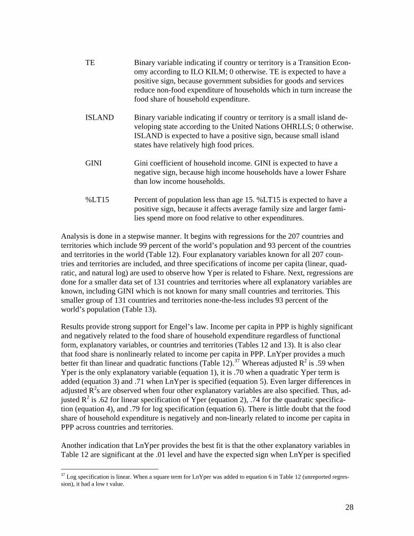
TE Binary variable indicating if country or territory is a Transition Econ-

omy according to ILO KILM; 0 otherwise. TE is expected to have a positive sign, because government subsidies for goods and services reduce non-food expenditure of households which in turn increase the food share of household expenditure.

ISLAND Binary variable indicating if country or territory is a small island de-

veloping state according to the United Nations OHRLLS; 0 otherwise. ISLAND is expected to have a positive sign, because small island states have relatively high food prices.

GINI Gini coefficient of household income. GINI is expected to have a

negative sign, because high income households have a lower Fshare than low income households.

%LT15 Percent of population less than age 15. %LT15 is expected to have a

positive sign, because it affects average family size and larger fami-lies spend more on food relative to other expenditures.

Analysis is done in a stepwise manner. It begins with regressions for the 207 countries and territories which include 99 percent of the world’s population and 93 percent of the countries and territories in the world (Table 12). Four explanatory variables known for all 207 coun-tries and territories are included, and three specifications of income per capita (linear, quad-ratic, and natural log) are used to observe how Yper is related to Fshare. Next, regressions are done for a smaller data set of 131 countries and territories where all explanatory variables are known, including GINI which is not known for many small countries and territories. This smaller group of 131 countries and territories none-the-less includes 93 percent of the world’s population (Table 13).

Results provide strong support for Engel’s law. Income per capita in PPP is highly significant and negatively related to the food share of household expenditure regardless of functional form, explanatory variables, or countries and territories (Tables 12 and 13). It is also clear that food share is nonlinearly related to income per capita in PPP. LnYper provides a much better fit than linear and quadratic functions (Table 12).37 Whereas adjusted R2 is .59 when Yper is the only explanatory variable (equation 1), it is .70 when a quadratic Yper term is added (equation 3) and .71 when LnYper is specified (equation 5). Even larger differences in adjusted R2s are observed when four other explanatory variables are also specified. Thus, ad-justed R2 is .62 for linear specification of Yper (equation 2), .74 for the quadratic specifica-tion (equation 4), and .79 for log specification (equation 6). There is little doubt that the food share of household expenditure is negatively and non-linearly related to income per capita in PPP across countries and territories. Another indication that LnYper provides the best fit is that the other explanatory variables in Table 12 are significant at the .01 level and have the expected sign when LnYper is specified

37 Log specification is linear. When a square term for LnYper was added to equation 6 in Table 12 (unreported regres-sion), it had a low t value.

28

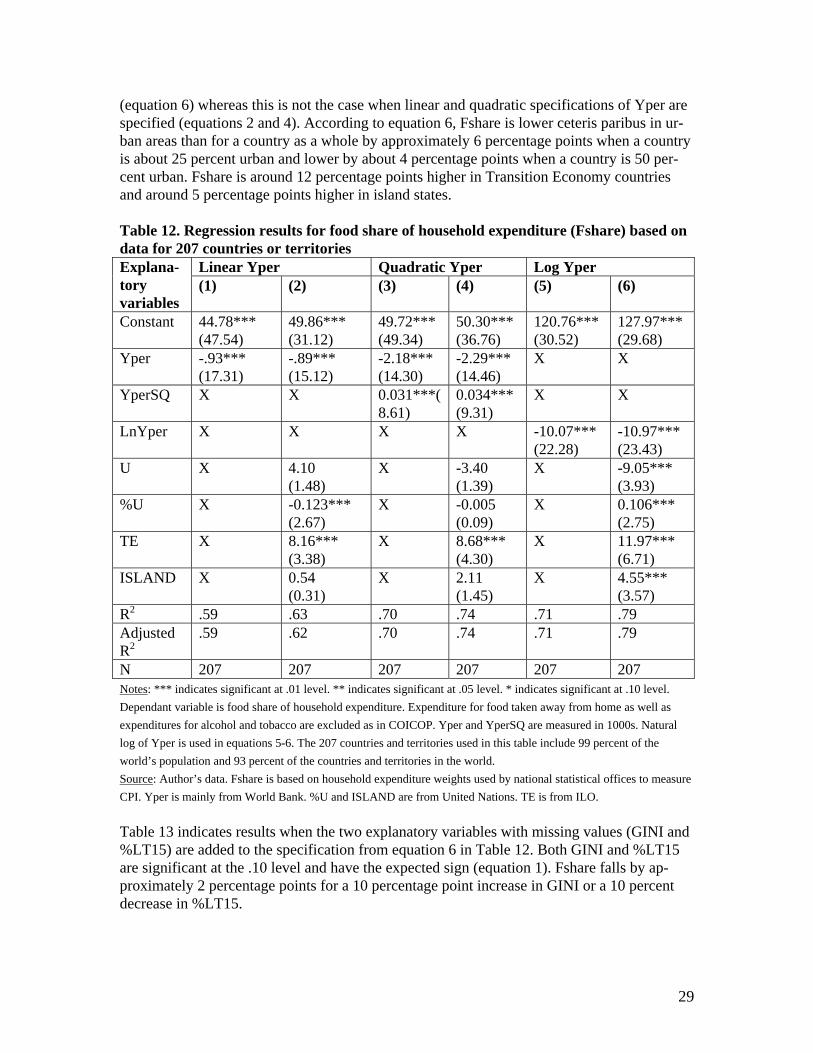
(equation 6) whereas this is not the case when linear and quadratic specifications of Yper are specified (equations 2 and 4). According to equation 6, Fshare is lower ceteris paribus in ur-ban areas than for a country as a whole by approximately 6 percentage points when a country is about 25 percent urban and lower by about 4 percentage points when a country is 50 per-cent urban. Fshare is around 12 percentage points higher in Transition Economy countries and around 5 percentage points higher in island states. Table 12. Regression results for food share of household expenditure (Fshare) based on data for 207 countries or territories

Linear Yper Quadratic Yper Log Yper Explana-tory variables

(1) (2) (3) (4) (5) (6)

Constant 44.78*** (47.54)

49.86*** (31.12)

49.72*** (49.34)

50.30*** (36.76)

120.76*** (30.52)

127.97*** (29.68)

Yper -.93*** (17.31)

-.89*** (15.12)

-2.18*** (14.30)

-2.29*** (14.46)

X X

YperSQ X X 0.031***(8.61)

0.034*** (9.31)

X X

LnYper X X X X -10.07*** (22.28)

-10.97*** (23.43)

U X 4.10 (1.48)

X -3.40 (1.39)

X -9.05*** (3.93)

%U X -0.123*** (2.67)

X -0.005 (0.09)

X 0.106*** (2.75)

TE X 8.16*** (3.38)

X 8.68*** (4.30)

X 11.97*** (6.71)

ISLAND X 0.54 (0.31)

X 2.11 (1.45)

X 4.55*** (3.57)

R2 .59 .63 .70 .74 .71 .79 Adjusted R2

.59 .62 .70 .74 .71 .79

N 207 207 207 207 207 207 Notes: *** indicates significant at .01 level. ** indicates significant at .05 level. * indicates significant at .10 level. Dependant variable is food share of household expenditure. Expenditure for food taken away from home as well as expenditures for alcohol and tobacco are excluded as in COICOP. Yper and YperSQ are measured in 1000s. Natural log of Yper is used in equations 5-6. The 207 countries and territories used in this table include 99 percent of the world’s population and 93 percent of the countries and territories in the world. Source: Author’s data. Fshare is based on household expenditure weights used by national statistical offices to measure CPI. Yper is mainly from World Bank. %U and ISLAND are from United Nations. TE is from ILO. Table 13 indicates results when the two explanatory variables with missing values (GINI and %LT15) are added to the specification from equation 6 in Table 12. Both GINI and %LT15 are significant at the .10 level and have the expected sign (equation 1). Fshare falls by ap-proximately 2 percentage points for a 10 percentage point increase in GINI or a 10 percent decrease in %LT15.

29

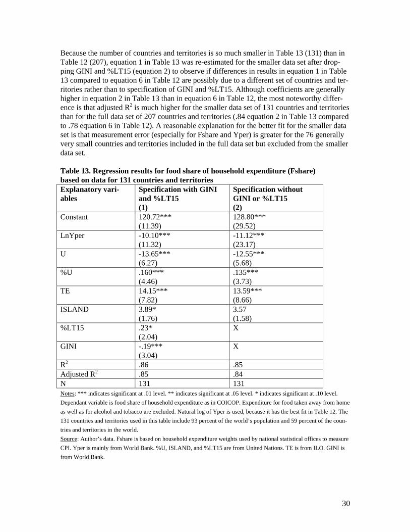
Because the number of countries and territories is so much smaller in Table 13 (131) than in Table 12 (207), equation 1 in Table 13 was re-estimated for the smaller data set after drop-ping GINI and %LT15 (equation 2) to observe if differences in results in equation 1 in Table 13 compared to equation 6 in Table 12 are possibly due to a different set of countries and ter-ritories rather than to specification of GINI and %LT15. Although coefficients are generally higher in equation 2 in Table 13 than in equation 6 in Table 12, the most noteworthy differ-ence is that adjusted R2 is much higher for the smaller data set of 131 countries and territories than for the full data set of 207 countries and territories (.84 equation 2 in Table 13 compared to .78 equation 6 in Table 12). A reasonable explanation for the better fit for the smaller data set is that measurement error (especially for Fshare and Yper) is greater for the 76 generally very small countries and territories included in the full data set but excluded from the smaller data set. Table 13. Regression results for food share of household expenditure (Fshare) based on data for 131 countries and territories Explanatory vari-ables

Specification with GINI and %LT15 (1)

Specification without GINI or %LT15 (2)

Constant 120.72*** (11.39)

128.80*** (29.52)

LnYper -10.10*** (11.32)

-11.12*** (23.17)

U -13.65*** (6.27)

-12.55*** (5.68)

%U .160*** (4.46)

.135*** (3.73)

TE 14.15*** (7.82)

13.59*** (8.66)

ISLAND 3.89* (1.76)

3.57 (1.58)

%LT15 .23* (2.04)

X

GINI -.19*** (3.04)

X

R2 .86 .85 Adjusted R2 .85 .84 N 131 131 Notes: *** indicates significant at .01 level. ** indicates significant at .05 level. * indicates significant at .10 level. Dependant variable is food share of household expenditure as in COICOP. Expenditure for food taken away from home as well as for alcohol and tobacco are excluded. Natural log of Yper is used, because it has the best fit in Table 12. The 131 countries and territories used in this table include 93 percent of the world’s population and 59 percent of the coun-tries and territories in the world. Source: Author’s data. Fshare is based on household expenditure weights used by national statistical offices to measure CPI. Yper is mainly from World Bank. %U, ISLAND, and %LT15 are from United Nations. TE is from ILO. GINI is from World Bank.

30

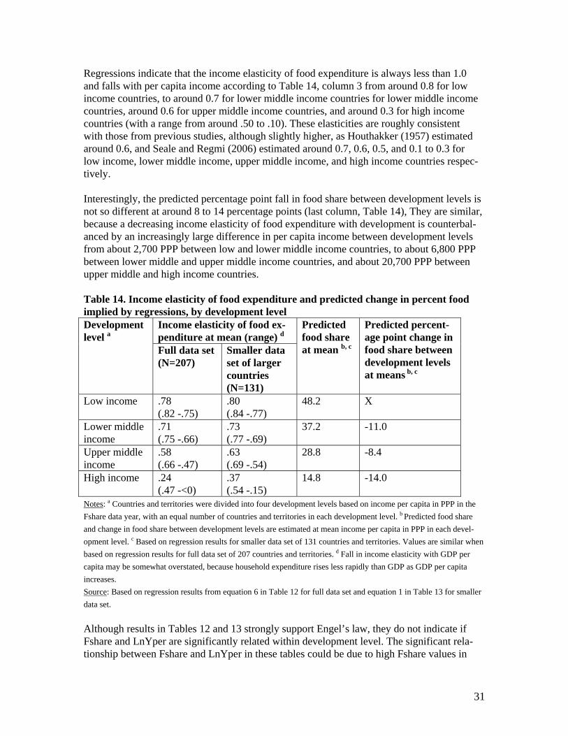
Regressions indicate that the income elasticity of food expenditure is always less than 1.0 and falls with per capita income according to Table 14, column 3 from around 0.8 for low income countries, to around 0.7 for lower middle income countries for lower middle income countries, around 0.6 for upper middle income countries, and around 0.3 for high income countries (with a range from around .50 to .10). These elasticities are roughly consistent with those from previous studies, although slightly higher, as Houthakker (1957) estimated around 0.6, and Seale and Regmi (2006) estimated around 0.7, 0.6, 0.5, and 0.1 to 0.3 for low income, lower middle income, upper middle income, and high income countries respec-tively. Interestingly, the predicted percentage point fall in food share between development levels is not so different at around 8 to 14 percentage points (last column, Table 14), They are similar, because a decreasing income elasticity of food expenditure with development is counterbal-anced by an increasingly large difference in per capita income between development levels from about 2,700 PPP between low and lower middle income countries, to about 6,800 PPP between lower middle and upper middle income countries, and about 20,700 PPP between upper middle and high income countries. Table 14. Income elasticity of food expenditure and predicted change in percent food implied by regressions, by development level

Income elasticity of food ex-penditure at mean (range) d

Development level a

Full data set (N=207)

Smaller data set of larger countries (N=131)

Predicted food share at mean b, c

Predicted percent-age point change in food share between development levels at means b, c

Low income .78 (.82 -.75)

.80 (.84 -.77)

48.2 X

Lower middle income

.71 (.75 -.66)

.73 (.77 -.69)

37.2 -11.0

Upper middle income

.58 (.66 -.47)

.63 (.69 -.54)

28.8 -8.4

High income .24 (.47 -<0)

.37 (.54 -.15)

14.8 -14.0

Notes: a Countries and territories were divided into four development levels based on income per capita in PPP in the Fshare data year, with an equal number of countries and territories in each development level. b Predicted food share and change in food share between development levels are estimated at mean income per capita in PPP in each devel-opment level. c Based on regression results for smaller data set of 131 countries and territories. Values are similar when based on regression results for full data set of 207 countries and territories. d Fall in income elasticity with GDP per capita may be somewhat overstated, because household expenditure rises less rapidly than GDP as GDP per capita increases. Source: Based on regression results from equation 6 in Table 12 for full data set and equation 1 in Table 13 for smaller data set. Although results in Tables 12 and 13 strongly support Engel’s law, they do not indicate if Fshare and LnYper are significantly related within development level. The significant rela-tionship between Fshare and LnYper in these tables could be due to high Fshare values in

31

low income countries together with low Fshare values in high income countries with data clouds at each development level. With this in mind, equation 6 in Table 12 and equation 1 in Table 13 were re-estimated for four development levels and ten per capita income deciles based on a country or territory’s income per capita in PPP in the data year for Fshare (Tables 15 and 16). Results in Table 15 continue to provide strong support for Engel’s law. LnYper is significant at the .01 level in all four development levels. At the same time, it is clear that part of the high R2 observed in Tables 12 and 13 is due to a comparison of high food shares in low in-come countries with low food shares in high income. Whereas adjusted R2 is .78 for the full data set, it ranges from .15 to .66 within the four development levels for the full data set. Similarly, whereas adjusted R2 for the smaller data set is .85, it ranges from .41 to .78 within development level for the smaller data set. As in Tables 12 and 13, R2 is considerably higher at each development level for the smaller data set than for the full data set, again probably due to greater measurement error for small countries and territories included in the full data set but not in the smaller data set. It is also worth noting that adjusted R2 is lower for low in-come and high income countries compared to middle income countries, especially for the smaller data set. A lower R2 for low income countries may be due to greater measurement error and noise for Fshare and Yper in low income countries. A lower R2 for high income countries may be due to unmeasured differences between countries being important relative to the low income elasticity of food expenditure in high income countries. Differences in results by development level for other explanatory variables in Table 15 are also generally consistent with a priori expectations, which adds confidence to the regressions results. U and %U are insignificant for high income countries and less important for upper middle income countries while being highly significant for low and lower middle income countries. This makes sense because differences between urban and rural areas in non-food needs and costs are great in lower income developing countries and small in higher income countries. ISLAND is similarly highly significant for low and lower middle income countries and insignificant for upper middle and high income countries. This might be due to a reduc-tion in transport costs for higher income small island states because of greater purchasing power. Results for TE are similar and significant across development level. On the other hand, results for GINI and %LT15 in Table 15 call into question results for them in Table 13 as GINI and %LT15 are only significant for lower middle income countries.

32

Table 15. Regression results for food share of household expenditure, by development level

Low income percapita in PPP

P P

Lower middle income per capita in PP

Upper middle in-come per capita in PP

High income per capita

Ex-plana-tory vari-ables a

set

Fulldata set

Smallerdata set

Fulldata set

Smaller data set

Full data set

Smaller data set

Full data

Smaller data set

Con-stant

149.44***

(6.38)

114.65***(342)

161.51***(5.55)

130.80*** (4.75)

109.73*** (4.75)

166.93*** (4.33)

94.97*** (3.66)

127.75*** (5.22)

LnYper -

-

14.00***(4.19)

10.99***(3.00)

-15.09***(4.22)

-11.21*** (3.44)

-9.11*** (3.72)

-14.18*** (3.79)

-7.72 *** (3.08)

-10.25*** (4.35)

U -

-

18.45**

*(3.54)

22.71***(4.34)

-2.47 (0.41)

-19.14*** (3.10)

-6.21 (1.52)

-8.29** (2.24)

7.15 (0.34)

3.30 (0.28)

%U .314**(2.10)

.352**(2.40)

.019 (0.15)

0.318*** (2.68)

.055 (1.00)

.067 (1.38)

-.062 (0.24)

-.053 (0.28)

TE 10.24**

(2.08)

16.27***(2.86)

10.93***(2.88)

12.85*** (3.62)

14.76*** (6.53)

10.73*** (4.13)

X X

IS-LAND

10.44***(2.86)

6.36(1.29)

8.59***(3.32)

X

1.30 (0.72)

X -1.70 (0.65)

X

GINI X

.02(0.88)

X -0.46** (4.39)

X -0.12 (0.77)

X -0.10 (0.97)

%LT15

X 0.31(0.88)

X 0.57*** (3.40)

X -0.19 (0.84)

X -0.26 (1.40)

R2 .39 .57 .38 .77 .69 .82 .22 .51 Ad-justed R2

.33 .46 .31 .71 .66 .78 .15 .41

N 52 37 52 29 51 34 52 31 Notes: *** indicates significant at .01 level. ** indicates significant at .05 level. * indicates significant at .10 level. Countries and territories were divided into four development levels based on income per capita in PPP in Fshare data year, with 52 or 51 countries or territories in each development level. Dependant variable is food share of household expenditure that excludes expenditure for food taken away from home and alcohol and tobacco even when national statistical office included these in food expenditure. a Binary explanatory variables are excluded from a regression when at this development level there were less than four such countries or territories. Source: Author’s data.

33

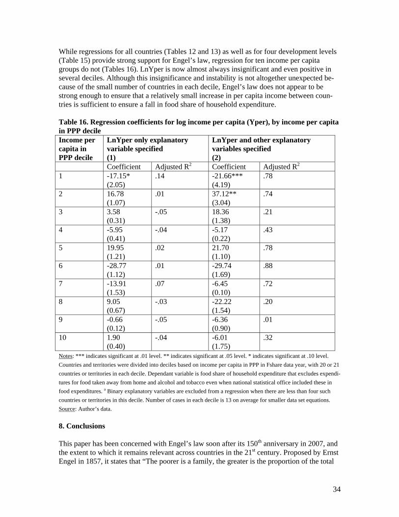
While regressions for all countries (Tables 12 and 13) as well as for four development levels (Table 15) provide strong support for Engel’s law, regression for ten income per capita groups do not (Tables 16). LnYper is now almost always insignificant and even positive in several deciles. Although this insignificance and instability is not altogether unexpected be-cause of the small number of countries in each decile, Engel’s law does not appear to be strong enough to ensure that a relatively small increase in per capita income between coun-tries is sufficient to ensure a fall in food share of household expenditure. Table 16. Regression coefficients for log income per capita (Yper), by income per capita in PPP decile Income per capita in PPP decile

LnYper only explanatory variable specified (1)

LnYper and other explanatory variables specified (2)

Coefficient Adjusted R2 Coefficient Adjusted R2 1 -17.15*

(2.05) .14 -21.66***

(4.19) .78

2 16.78 (1.07)

.01 37.12** (3.04)

.74

3 3.58 (0.31)

-.05 18.36 (1.38)

.21

4 -5.95 (0.41)

-.04 -5.17 (0.22)

.43

5 19.95 (1.21)

.02 21.70 (1.10)

.78

6 -28.77 (1.12)

.01 -29.74 (1.69)

.88

7 -13.91 (1.53)

.07 -6.45 (0.10)

.72

8 9.05 (0.67)

-.03 -22.22 (1.54)

.20

9 -0.66 (0.12)

-.05 -6.36 (0.90)

.01

10 1.90 (0.40)

-.04 -6.01 (1.75)

.32

Notes: *** indicates significant at .01 level. ** indicates significant at .05 level. * indicates significant at .10 level. Countries and territories were divided into deciles based on income per capita in PPP in Fshare data year, with 20 or 21 countries or territories in each decile. Dependant variable is food share of household expenditure that excludes expendi-tures for food taken away from home and alcohol and tobacco even when national statistical office included these in food expenditures. a Binary explanatory variables are excluded from a regression when there are less than four such countries or territories in this decile. Number of cases in each decile is 13 on average for smaller data set equations. Source: Author’s data. 8. Conclusions This paper has been concerned with Engel’s law soon after its 150th anniversary in 2007, and the extent to which it remains relevant across countries in the 21st century. Proposed by Ernst Engel in 1857, it states that “The poorer is a family, the greater is the proportion of the total

34

outgo [family expenditures] which must be used for food. … The proportion of the outgo used for food, other things being equal is the best measure of the material standard of living of a population” (Engel quoted in Zimmerman, 1932). Until recent decades, Engel’s law was seen as one of the most important relationships in economics. On its 75th anniversary, a major review article said “In the field of family consumption and expenditures, one theory attracts first attention above all others – the so-called Engel’s law” (Zimmerman, 1932). On its 100th anniversary, a major review article said “Few dates in the history of econometrics are more significant than 1857. In that year, Ernst Engel (1821-1896) published a study in which he formulated an empirical law concerning the relationship between income and expenditure on food” (Houthakker, 1957). At present though, Engel’s law is viewed more as a historical cu-riosity referred to in a footnote or noted in passing, despite the fact that many national pov-erty lines and therefore poverty rates are based in part on Engel’s law. The present study improves on previous cross-national studies of food expenditure. First, data for an unusually large number of countries and territories (207) are used. This makes it possi-ble to analyze how the relationship between the food share of household expenditure and in-come per capita differs by development level. Second, almost all food share estimates used are from national statistical offices based on household budget surveys whereas previous cross-national studies have generally relied on data from international organizations often based on SNA statistics. Estimates from national statistical offices are more likely to reflect local conditions and behavior and have not been adjusted in unknown ways by international organizations. In addition, SNA based estimates do not distinguish between expenditures by resident households and expenditures by tourists. Third, national reported food shares esti-mates were adjusted to increase cross-country comparability by subtracting expenditures for alcohol, tobacco and food taken away from home when a country or territory included these in food, which was often. Previous cross-national studies have generally accepted food share as reported. Fourth, regression analysis takes into consideration when a country’s food share estimate is based on data for urban households and not on a national sample which is com-mon, something which previous studies have not done. This is important, because food share is lower in urban areas than in rural areas. Fifth, analysis used income per capita in PPP for a country or territory for the same year as the food share estimate, something which previous studies have generally not done perhaps because they did not realize that food share estimates are always based on data from an earlier year (and often a much earlier year), especially for many developing countries. Sixth, recently revised 2007 and 2008 World Bank estimates of income per capita in PPP were used to measure material national standard of living, which were not available to previous cross-national studies. These new estimates are widely be-lieved to more accurately reflect differences in standards of living than earlier World Bank estimates. Evidence in this paper indicates that Engel’s law continues to be relevant, at the beginning of the 21st century. Within countries at the household level, evidence supporting Engel’s law is strong. Accord-ing to household survey data for 46 countries from around the world tabulated by income decile, food share of household expenditure fell across adjacent income deciles within each country so consistently that few exceptions were observed, and the same consistent result was found at all development levels and in all regions. Furthermore, the food share of household income was much lower among high income households compared to low income house-

35

holds. Food share was 21 percentage points lower on average in the bottom income decile compared to the top income decile, which is quite large given that average food share for all households was 29 percent. At the cross-national level, evidence supporting Engel’s law is also strong. According to na-tional food share estimates for 207 countries and territories, which represent 99 percent of the world’s population, food share of household expenditure fell from around 50 percent on av-erage in low income countries, to around 40 percent in lower middle income countries, around 30 percent in upper middle income countries, and around 15 percent in high income countries. Food share was significantly related to income per capita in PPP, even after speci-fication of measurement- and behavioral-related explanatory variables; as well, analysis in Appendix A indicates that results are similar when expenditure for food taken away from home is specified as an explanatory variable. Regressions are able to explain 80 to 85 percent of the variation in national food shares, and log of income per capita in PPP by itself explains around 70 percent of cross-national variation in food share. The effect of per capita income on food share was nonlinear, and the income elasticity of food expenditure fell from around 0.80 for an average low income country, to around 0.70 for an average lower middle income country, 0.60 for an average upper middle income country, 0.30 for an average high income country, and .10 for the highest per capita income countries. Additional confirmation of Engels’ law was provided by separate regressions for four development levels, especially given much smaller sample sizes, as log per capita income in PPP was significant in all four development levels. In summary, convincing evidence has been presented indicating that Engel’s law continues to be relevant today across countries as well as across households within countries. At the same time, the relationship between food share and per capita income is not strong enough to en-sure that food shares of countries with similar per capita incomes are necessarily consistent with Engel’s law. Also, the relationship between food share and per capita income is weak for countries with especially high per capita income. Thus while Engel’s law is still relevant on its 150th anniversary, it is only sufficient strong to predict differences in food shares of countries with reasonably large differences in per capita income.

36

Appendix A: Expenditure for food taken away from home and its effect on expenditure for food at home A potentially important problem with national food expenditure statistics, and therefore by extension for cross-national analysis of Engel’s law, is that countries differ in how they treat expenditure for food taken away from home (see Section 3.2.3). Although most countries in-clude expenditure for meals away from home in a separate expenditure group called “Restau-rants and hotels”, over 20 percent of countries and territories include this expenditure in food. While it is clear that a portion of expenditure for food taken away for home should be in-cluded in food expenditure because part of the cost of meals away from home is the food contained in these meals, it is also clear that a considerable part of the cost of a meal away from home is for services such as cooking, cleaning, serving, and food preparation. Unfortu-nately, not much information is available on the difference between cost of meals away from home and similar meals prepared at home, or on how this difference varies by country. Fur-ther complicating matters is that the percentage of household expenditure for food taken away from home is not known for most countries in the world. In light of the potential importance of expenditure for food taken away from home for an analysis of food expenditure, the present appendix looks in detail at expenditure for food taken away from home and how it is related to food expenditure as defined in this paper and by the standard international classification of household expenditure (COICOP) which ex-cludes it. Section A1 looks at the difference between cost of a meal eaten away from home and a similar meal prepared at home based on recent field work by the author. Section A2 presents new national estimates of the percentage of household expenditure for food taken away from home. Section A3 investigates how expenditure for food taken away from home is related to expenditure for food at home using regression analysis. A1. Difference between cost of meals away from home and similar meals prepared at home To get a rough idea of how large the difference is between cost of a meal away from home and cost of the same meal prepared at home, I purchased street food meals in Xian, China and restaurant meals in Springfield, Massachusetts USA. Street food meals in Xian China were noodles with vegetables and meat, and steamed buns with fillings. Meals in Springfield USA were Big Mac and One-quarter Pounder with small fries and medium coke in McDon-ald’s and 9 oz sirloin steak dinner with salad, baked potato and coke without dessert in Out-back Steakhouse, a basic sit down restaurant.38 After purchasing meals, I took them apart and weighed their contents. I also looked on the web for recipes for McDonald’s sauces. Next, I priced all food items included in these meals in markets where workers shop. In this way, I was able to estimate cost of the food contained in these meals and therefore their cost if they were prepared at home. I estimated that street food meals in Xian China cost roughly between 10-30 percent more than similar meals pre-

38 McDonald’s and Outback Steak House were chosen for the United States, because they serve standardized meals with information on what is included in their meals. This facilitated ascertaining the cost of the food included in these meals.

37

pared at home.39 Cost of food in a McDonald’s meal was estimated to be around 40 percent of its cost in McDonalds. Cost of food in an Outback Steak House meal was estimated to be around 30 percent of its cost in Outback Steakhouse. 40 My estimates for the United States are consistent with a rule of thumb used in the restaurant business in the United States that around one-third of the cost of a meal is for food (Lawrence, 1992). 41 Since the above rough estimates of mine are based on an analysis of relatively inexpensive meals, they undoubtedly understate the average difference for a country, as the cost of expen-sive meals should be greater compared to the cost of preparing the same meal home than are inexpensive meals. This means that the average difference for China is more likely to be somewhere around 20-30 percent and for the United States somewhere around 70-75 percent in my opinion. The smaller difference for China compared to the United States makes sense, because the difference in labor costs between lower and higher income countries is greater than the difference in the cost of food between lower and higher income countries as food is internationally traded while labor is not.42, 43 While the above estimates of cost differences between meals taken away from home and similar meals prepared at home for China and the United States are only rough estimates for one city and several “restaurants” in each country, they are none-the-less informative. They indicate that: (i) cost of the food contained in a meal taken away from home is considerably less than the cost of a similar meal prepared at home; (ii) difference between cost of a meal away from home and cost of food in the meal varies by country and probably development level; (iii) knowledge is limited on this topic. A2. National estimates of expenditure shares for food taken away from home Systematic information on household expenditure for food taken away from home was not available when I began this paper. 44 Nor were there cross-national analyses on how expendi- 39 The large range for Xian, China reflects that street market meals in China are far from standardized. 40 One reason for the difference between Outback Steak House and McDonald’s is that customers are expected to leave a 15 percent tip for the server in Outback Steak House whereas McDonalds is self-service. 41 Note that since there is usually a state (and sometimes city) sales tax for restaurant meals in the United States (gener-ally around 5 percent) but no sales tax on most food purchased in supermarkets, this would cause the cost of a meal in the United States for consumers to be five percent higher than the usual rule of thumb used by restaurants ceteris pari-bus. Also, restaurant owners do not consider the cost of a tip for a server. 42 According to food price data for over 100 countries or territories provided on an ILO website (www.laborsta.ilo.org), the average per kg cost in 2005 of white wheat flour (a food with similar quality around the world) was almost the same in developing countries and territories as in the United States (68 and 69 cents respectively), although the per kg price of white wheat flour was considerably lower in two developing regions (27 cents in South Asia and 51 cents in North Africa and Middle East on average). 43 Although speculative, it also seems reasonable to expect the difference between the cost of a meal eaten away from home and a similar meal prepared at home to be smaller ceteris paribus in countries where people frequently eat away from home compared to countries where people do not often eat away from home. For example, cost of a meal in an American McDonalds’ restaurant should be closer to the cost of the food in the meal compared to a restaurant meal in France. One should expect the relative cost of meals away from home to fall as the cost of services for meals is reduced through self-service, as profit margins are reduced through increased competition, and as input costs are reduced through bulk purchase. 44 ICP and EUROSTAT provide estimates of expenditure for restaurants and hotels. These data are not used, because they have major problems for the regression analysis in this paper. First and most importantly, ICP and EUROSTAT estimates are often based on SNA data and so include expenditure of foreign tourists and cross-border persons in addi-tion to expenditure of residential households. This can greatly affect national estimates, especially in countries and territories with a large tourist sector or considerable cross-border work and shopping. UK and Luxembourg data illus-

38

ture for food taken away from home affects household expenditure for food at home. Given this weak knowledge base together with the potentially important affect expenditure for food taken away from home might have on expenditure for food at home, I put in considerable effort to develop a data set of national expenditure shares for food taken away from home. How this was done is described in the remainder of this section. I found expenditure shares for food taken away from home for 98 countries or territories, al-most always from national a statistical office based on a household budget survey. This in-cluded 47 countries or territories which include expenditure for food taken away from home in food expenditure, and 51 countries or territories which do not include expenditure for food taken away from home in food expenditure but for whom a value was none-the-less found, often for an earlier year. This meant that the expenditure share for food taken away from home was unknown for 109 countries and territories. Median national values for a country’s region was used to impute a value for these 109 countries and territories based on available national values in my data set for other countries and territories in the region (Table A1). Median values were: 1.4 for Sub-Sahara Africa, 1.4 for Pacific Islands, 1.6 for Middle East and North Africa, 1.9 for Transi-tion Economies, 2.3 for Caribbean, 5.2 for Europe and Developed, 5.7 for South America, 6.4 for Central America, 7.6 for East Asia, and 10.3 for South-East Asia. Since only one national estimate was available in my data set for South Asia, median ICP estimates of restaurant and hotel expenditure for countries in South Asia was used after reducing this somewhat to take into account hotel expenditures; this yielded an estimate of 1.2 percent for South Asia.

trate how misleading SNA data can be. Whereas expenditure for restaurants and hotels represent 10.3 percent of total expenditure by individuals in UK and 7.3 percent of total expenditure by individuals in Luxembourg according to SNA statistics, expenditure for food taken away from home represent 4.7 percent of resident household expenditure in UK and 5.0 percent of resident household expenditure in Luxembourg according to household budget data (Wingfield, 2007 for UK; Luxembourg STATEC, 2003 for Luxembourg). ICP data for Africa illustrate for developing countries how much tourism can affect the percentage of household expenditure for restaurant and hotels. Of the seven African countries with an expenditure share above 5 percent for restaurants and hotels in ICP data (out of 30 African countries with data), 4 have a large tourism sector: Tunisia (17.2 percent of expenditure are for restaurants and hotels), Morocco (8.1 percent), Kenya (5.8 percent), and Mauritius (5.3 percent) (African Development Bank, 2007). Second, expendi-ture for alcoholic beverages consumed in restaurants and cafes is included in restaurant expenditure. This undoubtedly helps explain at least partly why expenditure for food taken away from home is estimated to represent 17.1 percent of household expenditure in Ireland. Third, expenditure for restaurants and hotels is reported as one expenditure group in ICP data.

39

Table A1. Information on expenditure share for food taken away from home, by region Region/Sub-region Number (%)

include food taken away from home in food expendi-ture

Number (%) with known value for food taken away from home ex-penditure

Median per-cent food taken away from home expenditure (when known)

Sub-Saharan Africa (N=45) 5 (11.1%) 17 (37.8%) 1.4 East Asia (N=6) 4 (75.0%) 6 (100.0%) 7.6 South-East Asia (N=11) 7 (63.6%) 7 (63.6%) 10.3 South Asia (N=8) 1 (12.5%) 1 (12.5%) 1.2a Central America (N=8) 2 (25.0%) 5 62.5%) 6.4 South America (N=12) 7 (58.3%) 11 (91.7%) 5.7 Caribbean (N=21) 2 (9.5%) 7 (33.3%) 2.3 Middle East and North Af-rica (N=20)

3 (15.0%) 7 (35.0%) 1.6

Pacific Islands (N=15) 5 (33.3%) 6 (4.0%) 1.4 Transition Economy (N=19) 1 (5.3%) 4 (9.5%) 1.9 Developed and Europe (N=42)

9 (21.4%) 27 (64.3%) 5.2

Total (N=207) 47 (22.7%) 98 (47.3%) 4.5 Notes: More regions are included in this table than in tables in main text. Additional regions are included when there were large and consistent differences between sub-regions within a region (e.g. for Latin America and Asia). a Value for South Asia is based on ICP data, because there was only one national value in author’s data set for South Asia. Source: Author’s data based on national estimates from national statistical offices except for South Asia (see a). A3. Regression analysis of affect expenditure for food taken away from home has on expenditure for food at home This section uses regression analysis to investigate the relationship between expenditure for food taken away from home and expenditure for food at home - - in particular, extent to which expenditure for food taken away from home systematically reduces expenditure for food at home. As in Section 6.2, share of household expenditure for food at home (Fshare) is the dependant variable. Different from Section 6.2 is that food taken away from home (Faway) is included as an explanatory variable in this appendix. A priori expectation is that Faway will be nega-tively related to Fshare, since expenditure for food taken away from home should reduce the need for expenditure for food at home. Although there are no previous studies to indicate the magnitude of this affect, the author’s recent fieldwork in China and United States on the dif-ference in the cost of a meal purchased away from home and a similar meal prepared at home (see Section A1) suggests a coefficient of somewhere around -0.4. This exploratory work also indicates that the negative effect of a unit increase in Faway on Fshare should decrease with per capita income, because the difference between the cost of meals purchased away

40

from home and similar meals prepared at home probably increases with per capita income (see Section A1).45 Faway Percentage of household expenditure for food taken away from home. Faway

is expected to have a negative sign, because expenditure for food taken away from home reduces the need for expenditure for food at home. Coefficient of somewhere around -0.4 is expected in keeping with discussion in Section A1.

Regressions were estimated for the full data set of 207 countries and territories and the smaller data set of 131 countries and territories, because results in Section 6.2 were some-what sensitive to the sample of countries or territories. Regressions were also estimated sepa-rately for countries and territories where Faway is known and not imputed to avoid possible biases associated with using an exploratory variable whose value is imputed for so many countries and territories (equations 2 and 4 in Table A2). R2 is expected to be higher in equa-tions 2 and 4 compared to equations 1 and 3, because Faway is measured with greater preci-sion in equations 2 and 4. Regression results provide some evidence that Faway systematically reduces Fshare. Faway is significant with a coefficient of -0.33 for the full sample of 207 countries and territories (equation 1) and with a coefficient of -0.42 for the 98 countries or territories where Faway is known and not imputed (equation 2).46 The size of these coefficients is consistent with results from the author’s recent fieldwork in China and United States. Also as hypothesized, R2 is higher when regressions are estimated for countries and territories with a known Faway value (equation 2 compared to equation 1; and equation 4 compared to equation 3). On the other hand, Faway is not significant and has a coefficient of only -.08 when regressions are esti-mated for the smaller set of countries and territories (equation 3 and 4). Interestingly, since residuals are generally negative for countries in the three developing sub-regions where Faway is high (East Asia, South-East Asia, and South America), it may be that to find an ef-fect of Faway on Fshare that both Faway and percentage of the cost of a meal away from home for food need to be high. In conclusion, regressions provide evidence that expenditure for food at home is negatively related to expenditure for food away from home as expected. This effect, however, is sensi-tive to the sample of countries and territories used to estimate it. Worth noting is that Faway does not have a major effect on coefficients of other explanatory variables (see coefficients in equation 1 in Table A2 compared to equation 6 in Table 12; and equation 3 in Table A2 compared to equation 1 in Table 13). Further data gathering and analysis of Faway is war-ranted in light of its potentially importance affect on Fshare. Further analysis should include a careful consideration of the influence that culture, climate and history have on expenditure for food away from home.

45 In an attempt to capture this effect, an interaction term of Faway and log income per capita in PPP was added to re-gressions in Table A2. It had an unexpected negative sign possibly because it picked up part of the high correlation between Fshare and LnYper. 46 It is interesting to note that when Faway is included in Fshare and used as the dependant variable in equation 6 in Table 12 and equation 1 in Table 13, the overall fit is much weaker. Adjusted R2 is only .31 and .23 compared to .79 and .85 in these tables. This indicates that it is not appropriate to include all of Faway in food expenditure when inves-tigating Engel’s law.

41

Table A2. Regression results for food share of household expenditure (Fshare) when share of household expenditure for food taken away from home (Faway) is specified as an explanatory variable

Full samples Smaller samples Explanatory variables

(1) a (2) (3) a (4) Constant 129.97***

(29.33) 111.80*** (19.61)

122.19*** (11.40)

116.84*** (10.09)

LnYper -10.70*** (21.78)

-9.28*** (15.47)

-10.17*** (11.13)

-9.51*** (9.72)

U -9.25*** (4.03)

-2.27 (0.61)

-14.09*** (6.37)

-7.76*** (2.97)

%U .109*** (2.91)

.036 (0.95)

0.167*** (4.55)

.110*** (3.14)

TE 11.33*** (6.25)

10.57*** (3.68)

13.79*** (7.39)

10.47** (3.91)

ISLAND 4.14*** (3.21)

4.92*** (3.06)

3.97* (1.79)

3.20 (1.48)

GINI X X -.19*** (3.03)

-.29*** (4.09)

%LT15 X X .21** (1.93)

.27* (1.96)

Faway -.33* (1.74)

-.42** (2.30)

-.08 (0.40)

-.08 (0.40)

R2 .79 .85 .86 .90 Adjusted R2 .79 .84 .85 .89 N 207 98 131 72 Notes: *** indicates significance at .01 level; ** indicates significance at .05 level; * indicates significance at .10 level. a Includes 109 countries or territories whose Fshare value was imputed based on regional average (median) Faway val-ues for countries or territories with known values. Source: Author’s data drawn from national sources.

42

References African Development Bank. 2007. Comparative Consumption and Price Levels in Afri-can Countries: First Results of the International Comparison Program for Africa, Main Report. ADBG. Tunis. AFRISTAT. 2002. Evolution des Prix dans les Etats Membres d’AFRISTAT de 1970-1999. Serie Etudes No. 4. Bamako. Available on: www.afristat.org/contenu/pdf/rsc/pubprix_tot.pdf. Anker, R. 2005. A new methodology for estimating internationally comparable poverty lines and living wage rates. ILO Policy Integration Department Working Paper No. 72. ILO. Geneva. Asian Development Bank. 2007. Purchasing Power Parities and Real Expenditures: In-ternational Comparison Program in Asia and the Pacific. ADB. Manila. Asra, A. and Santos-Francisco, V. 2001. Poverty lines: Eight countries’ experiences and the issue of specificity and consistency. Paper presented at the Asian-Pacific Forum on Poverty. ADB. Manila. 5-9 February. Bhalotra, A. and Attfield, C. 1998. Intrahousehold resource allocation in rural Pakistan: A semi-parametric analysis. Journal of Applied Econometrics. Vol. 13, pp 463-480. CIA. 2008. World Factbook. www.cia.gov/library/pubications/the-world-factbook. ECLAC. 2007. Final results of the International Comparison Program for South Amer-ica, 2005. ECLAC. Santiago. EUROSTAT.2008. Harmonized Indices of Consumer prices (HICP). epp.eurostat.ec.europa.eu. Herrmann, S. and Polgar, E.K. 2007. Understanding price and consumption price indices in South-East Europe. ECB Occasional Paper Series No. 57. March. Houthakker, H. S. 1957. An international comparison of household expenditure patterns, commemorating the centenary of Engel’s law. Econometrica. Vol. 25 No. 4 (Oct), pp 532-551. IBGE. 2005. Armonizacion de los Indicesde Precios al Consumidor de los paises del MERCOSUR y Chile. IBGE. Rio de Janeiro. ILO. 2009. Retail food prices database. www.laborsta.ilo.org. ILO. 2007. Household income and expenditure survey database. www.laborsta.ilo.org. ILO. 2004. Consumer Price Index Manual: Theory and Practice. ILO. Geneva.

43

ILO. 1992 and 1999. Sources and Methods: CPI. Vol. 1. ILO. Geneva, and www.laborsta.ilo.org for metadata. ILO KILM. 2007. Key Indicators of the Labor Market. ILO. Geneva. IMF. 2007. Online CPI metadata. www.dsbb.imf.org. Interest.com. 2009. How much house can you afford? www.interest.com/mortgage. Kedir, A. and Sourafel, G. 2007. Quadratic Engel curves with measurement error: Evidence from a budget survey. Oxford Bulletin of Economics and Statistics. Vol. 69. No. 1(Dec). pp 123-138. Lawrence, E. 1992. The Complete Restaurateur. Plume. New York. Luxembourg STATEC. 2003. “Indices des prix a la consummation – Developpements meth-odologiques de 1990 a 2003”. Bulletin du STATEC. OECD. 2007. CPI metadata. stats.oecd.org/metadata. Orshansky, M. 1969. How Poverty is Measured. Monthly Labor Review. Vol. 92. No. 2. pp. 37–41. Perthel, D. 1975. Engel’s law revisited. International Statistical Review. Vol. 43, No. 2, pp 211-218. Prais, S. J. and Houthakker, H. S. 1955. Reprinted in 1971. Family Budgets. Cambridge University Press. Cambridge. Sainz,P. 1994. The evolution of poverty in Latin America in the 1980s. Poverty Monitoring: an International concern. van der Hoeven, R. and Anker, R. (eds). St. Martins Press. New York. Seale, J. L. and Regmi, A. 2006. Modeling international consumption patterns. Review of Income and Wealth. Series 52. No. 4. Shiller, R. J. 2008. The Subprime Solution. Princeton University Press. Princeton. Statistics South Africa. 2002. Consumer Price Index: 2000 Weights. Statistical Release P0141.5. Turvey, R. 1979. Consumer Price Indices: An ILO Manual. Geneva. ILO. United Nations, Office of the High Representative for Least Developed Countries and Small Island Developing States. List of Small Island Developing States. www.un.org/special-rep/ohrlls/sids/list.html. United Nations, Statistical Division. 2008. Online database. unstats.un.org/unsd.

44

45

Wingfield, D. 2007. CPI and RPI: The 2007 basket of goods and services. Economic and Labour Monthly Review. Vol. 1, No. 4. World Bank. 2008. World Development Indicators. www.worldbank.org/data. World Bank. 2008a. 2005 International Comparison Program Global Results: Summary Tables of Results. World Bank. Washington DC. Wright, C. D. 1989. Comparative Wages, Prices and Cost of Living. Reprint of 16th An-nual Report of the Massachusetts Bureau of Statistics and Labor for 1885. Wright and Potter Printing Co. 1889. Boston. Zimmerman, C. 1932. “Ernst Engel’s law of expenditures for food”. The Quarterly Journal of Economics. Vol. 47, No. 1 (Nov.), pp 78-101.