Reserve Bank of Australia

Reserve Bank of AustraliaEconomic Research Department

2007

-01

RESEARCHDISCUSSIONPAPER

A Structural Model of Australia as a Small Open Economy

Kristoffer Nimark

RDP 2007-01

A STRUCTURAL MODEL OF AUSTRALIA AS A SMALLOPEN ECONOMY

Kristoffer Nimark

Research Discussion Paper2007-01

February 2007

Economic Research DepartmentReserve Bank of Australia

The author thanks Jarkko Jaaskela, Christopher Kent, Mariano Kulish, Philip Liuand Bruce Preston for valuable comments and discussions. The views expressedin this paper are those of the author and do not necessarily reflect those of theReserve Bank of Australia.

Author: nimarkk at domain rba.gov.au

Economic Publications: ecpubs@rba.gov.au

Abstract

This paper sets up and estimates a structural model of Australia as a small openeconomy using Bayesian techniques. Unlike other recent studies, the paper showsthat a small micro-founded model can capture the open economy dimensions quitewell. Specifically, the model attributes a substantial fraction of the volatility ofdomestic output and inflation to foreign disturbances and matches the evidencefrom reduced-form studies. In addition, the model relies much less than otherestimated models on a persistent shock to the risk premium to explain changesin the nominal exchange rate. The paper also investigates the effects of variousexogenous shocks on the Australian economy.

JEL Classification Numbers: E30, F41Keywords: small open economy, Australia, Bayesian methods

i

Table of Contents

1. Introduction 1

2. A Small-scale Model of Australia 2

2.1 Household Preferences 3

2.2 The Consumption Bundle 4

2.3 Import Demand 4

2.4 The Domestic Budget Constraint and International FinancialFlows 5

2.5 Firms 6

2.6 Export Demand 8

2.7 The World Economy 9

2.8 Monetary Policy 9

3. Estimation Strategy 10

3.1 Mapping the Model into Observable Time Series 11

3.2 Computing the Likelihood 14

3.3 The Data 15

4. Estimation Results 16

4.1 Model Fit 17

4.2 The Open Economy Dimension of the Model 19

4.3 The Impact of a Monetary Policy Shock 22

4.4 The Impact of Export Demand and Income Shocks 23

4.5 The Impact of a Productivity Shock 26

5. Conclusion 27

Appendix A: The Linearised Model 29

References 31

ii

A STRUCTURAL MODEL OF AUSTRALIA AS A SMALLOPEN ECONOMY

Kristoffer Nimark

1. Introduction

This paper presents and estimates a small structural model of the Australianeconomy with the aim of providing both a theoretically rigorous framework aswell as rich enough dynamics to make the model empirically plausible. Theeconomics of the model are simple. Households choose how much to consume andhow much labour to supply. Firms choose prices and then produce enough goodsto meet demand. A fraction of the domestically produced goods are exported anda fraction of the domestically consumed goods are imported, with the size of thefractions determined by the relative price of goods produced at home and abroad.This is the minimal structure needed to capture the open economy dimension ofthe Australian economy, and it is similar to that used in many other studies, forexample Lubik and Schorfheide (forthcoming), Galı and Monacelli (2005) andJustiniano and Preston (2005). In addition to this basic structure, the model isamended to account for the importance of the commodities sector for Australianexports by adding exogenous export demand and income shocks.

Estimated models derived from micro foundations have become popular tools atcentral banks around the world. One often-cited reason for this is that structuralmodels can be used to produce counterfactual scenarios, as well as to makepredictions about how macroeconomic outcomes would change if alternativepolicies were implemented. Nessen (2006) provides a useful perspective on howsmall structural models can be used in the policy process. She argues that amodel is not a tool that provides answers to questions, but rather a frameworkof principles in which a structured and transparent analysis can be conducted.

For any model to be a useful analytical tool, however, one first needs to establishwhether it provides a reasonable description of the data. In a series of papers,Smets and Wouters (2003, 2004) show that medium-scale models can fit thedynamics of a large (closed) economy well. Some recent papers have asked

2

whether structural open economy models can provide a similarly good fit.1

Particularly, Justiniano and Preston (2005) question whether these models canaccount for the influence of foreign shocks on the domestic economy. Thispaper shows that the influence of foreign shocks can indeed be captured by thedynamics of a small structural model. In addition to matching the magnitude of theinfluence of foreign shocks found by reduced-form methods, the model presentedhere can also explain a larger fraction of the nominal exchange rate variabilityendogenously than previous studies.2

The model is estimated using Bayesian methods that exploit informationfrom outside the data sample to generate posterior estimates of the structuralparameters. The number of time series used is larger than in most other studiesto ensure that the data span the open economy dimension of the model. Themagnitude of measurement errors in some of the observable time series used isalso estimated. This not only allows for errors in the data introduced through thedata collection process, but also recognises the fact that some of the theoreticalvariables of the model do not have clear-cut observable counterparts. Thisapproach also allows something to be said about how well these time series fitthe cross-equation and dynamic implications of the model.

2. A Small-scale Model of Australia

The structural model is in most respects a standard New Keynesian small openeconomy model. But the model has a number of adjustments to account for somefeatures of the Australian economy that are peculiar compared to many otherdeveloped countries. In particular, while international trade for most developedcountries appears be driven by benefits that come from specialisation, Australia’sexternal trade appears to be driven more by classical comparative advantage, withexports dominated by primary products, while more than half of imports aremanufactured goods.3 In the standard model, the demand for a country’s exportsare determined by the level of world output and the domestic relative cost of

1 See, for instance, Justiniano and Preston (2005) and Fukac, Pagan and Pavlov (2006).

2 See Lubik and Schorfheide (2005), Linde, Nessen and Soderstrom (2004) and Justiniano andPreston (2005).

3 See Department of Foreign Affairs and Trade (2005).

3

production. Australia can be considered to be a price taker in many of its exportmarkets and has little influence over the price of its exports. Exogenous shocksare therefore added to both the volume of export demand as well as the price thatexporters receive for their goods.

Australia is also considered asmall economy in the model in the sense thatmacroeconomic outcomes and policy in Australia are assumed to have nodiscernable impact on world output, inflation and interest rates. These foreignvariables are thus modelled as being exogenous to Australia.

2.1 Household Preferences

A continuum of households populate the economy, consume goods and supplylabour to firms. Consider a representative household indexed byi ∈ (0,1) thatwishes to maximise the discounted sum of its expected utility

Et

∞∑s=0

βsU(Ct+s(i),Nt+s(i)

)(1)

whereβ ∈ (0,1) is the household’s subjective discount factor. The period utilityfunction in consumptionCt and labourNt is given by

U (Ct(i),Nt(i)) =

(Ct(i)H

−η

t

)1−γ

(1− γ)− Nt(i)

1+ϕ

1+ϕ(2)

and reflects the fact that households like to consume but dislike work. ThevariableHt

Ht =∫

Ct−1(i) di (3)

is a reference level of consumption capturing the notion that households not onlycare about their own consumption, but also care about the lagged consumptionof others. This feature – often referred to as ‘external habits’ or a preference for‘catching up with the Joneses’ – helps to explain the inertia of aggregate output,since past levels of aggregate consumption are positively related to the marginalutility of current consumption under this set-up.

4

2.2 The Consumption Bundle

Households’ preferences are specified over a continuum of differentiated goodsthat enter the households’ utility function with decreasing marginal weight.Households thus prefer to consume a mixture of differentiated goods rather thanconsuming just one variety. The consumption bundleCt is a constant elasticityof substitution (CES) aggregated index of domestically produced and importedsub-bundlesCd

t andCmt

Ct ≡[(1−α)

1δ C

dδ−1δ

t +α1δ C

mδ−1δ

t

] δ

1−δ

(4)

Cdt =

[∫Cd

t ( j)ϑ−1

ϑ d j

] ϑ

ϑ−1

(5)

Cmt =

[∫Cm

t ( j)ϑ−1

ϑ d j

] ϑ

ϑ−1

(6)

The domestic price index (CPI) that is consistent with the specification of theutility function is then given by

Pt =[(1−α)Pd1−δ

t +αPm1−δ

t

] 11−δ

(7)

This specification implies that in steady state, domestichouseholds spend a fraction(1−α) of their income on domestically produced goods.

2.3 Import Demand

The domestic demand for imported goodsCmt can be shown to be

Cmt = Ct exp(vm

t )(expτt)−δ (8)

which depends on the relative price of importsτt as perceived by the domesticconsumer

τt = log

(Pm

t

Pt

)(9)

Thus, the cheaper are imported goods relative to domestic goods, the larger willbe the share of imported goods in the consumption bundle. The exogenous shock

5

vmt to the domestic consumers’ demand for imported goods is assumed to follow

an AR(1) process

vm = ρmvmt−1+ ε

mt (10)

εmt ∼ N(0,σ2

m) (11)

The exogenous shock is needed to match the data, but ideally should only explaina small portion of the dynamics of imports.

2.4 The Domestic Budget Constraint and International Financial Flows

The representative household optimises the utility function (1) subject to its flowbudget constraint

Bt+1+B∗t+1+Ct −ψ

2B∗2

t = Yt +(expvpxt −1)Xt +Rt

Pt−1

PtBt +

StPt−1R∗t B∗tSt−1Pt

(12)

The variables on the left-hand side are expenditure items and the terms on theright-hand side are income items.Bt(i) andB∗t (i) are domestic and foreign bonds,respectively, where both are expressed in real domestic terms. Their respectivenominal returns areRt and R∗t . St is the nominal exchange rate defined suchthat an increase inSt implies a depreciation of the domestic currency. The termψ

2 B∗2t is a cost paid by domestic households when they are net borrowers in the

aggregate.4 This ensures that the net asset position of the domestic economy isstationary and it implies that,ceteris paribus, a highly indebted country will havea higher equilibrium interest rate.Yt on the right-hand side is real GDP and theterm(expvpx

t )Xt is export income adjusted for exogenous fluctuations in the priceof exports (more on this below).

Assuming a zero net supply of domestic bonds we can write the flow budgetconstraint as a difference equation describing the evolution of the net foreign assetposition

B∗t+1 =StPt−1R∗t B∗t

St−1Pt+

ψ

2B∗2

t +(expvpx

t

)Xt −Cm

t (13)

where the change in the net foreign asset position is the difference betweenincome received for exports and expenditure on imports plus valuation effects

4 See Benigno (2001).

6

from inflation and changes in the nominal exchange rate and the net debtor costψ

2 B∗2t . Households choose consumption subject to the flow budget constraint given

by Equation (12). Optimally allocating consumption over time yields the standardconsumption Euler equation

Uc(Ct) = βEtRtPtUc(Ct+1)

Pt+1(14)

whereUc(Ct) is the marginal utility of consumption in periodt. Households alsochoose between allocating their savings to bonds denominated in the domestic andforeign currency. Equating the marginal expected return on foreign and domesticbonds yields the uncovered interest rate parity (UIP) equilibrium condition

Rt =(expvs

t

)Et

R∗tψB∗t

St

St+1(15)

wherevst is a time-varying ‘risk premium’ that is assumed to follow the AR(1)

process

vst = ρsv

st−1+ ε

st (16)

εst ∼ N

(0,σ2

s

)(17)

The time-varying and persistent risk premiumvst is usually necessary to account

for the observed deviations of the exchange rate from that implied by the UIPcondition. There is no consensus in the literature on the causes of the deviationsand the interpretation of the risk premium shock does not have to be literal.5

2.5 Firms

The domestic economy is populated by two types of firms: producers andimporters. Domestic producers indexed byj use labour as the sole input tomanufacture differentiated goods with a linear technology

Yt( j) = exp(at)Nt( j) (18)

5 See, for instance, Bacchetta and van Wincoop (2006) for an explanation based on informationimperfections.

7

whereat is a sector-wide exogenous process that augments labour productivityassumed to follow

at = ρaat−1+ εat (19)

εat ∼ N

(0,σ2

a

)(20)

In addition to the production sector, there is a sector that imports differentiatedgoods from the world and resells them domestically.

Firms have some market power over the price of the goods that they are sellingsince consumers prefer a mixture of differentiated goods rather than consumingjust one variety. Unlike the case when all goods are perfect substitutes, this meansthat consumers will not switch consumption away completely from a slightly moreexpensive good. In this monopolistically competitive environment firms charge amark-up over marginal cost.

Quantities sold in a given period are demand-determined in the sense that firms areassumed to set prices in domestic currency terms and then supply the amount ofgoods that are demanded by consumers at that price. Both importers and domesticproducers set prices according to a discrete time version of the Calvo (1983)mechanism whereby a fractionθd of firms producing domestically and a fractionθ

m of importing firms do not change prices in a given period. A fractionω of boththe domestic producers and importers that do change prices, use a rule of thumbthat links their price to lagged inflation (in their own sector). This is a two-sectorgeneralisation of Galı and Gertler (1999) that yields two Phillips curves of thefollowing form

πdt = µ

df Etπ

dt+1+ µ

dbπ

dt−1+λ

dmcdt +vπ

t (21)

andπ

mt = µ

mf Etπ

mt+1+ µ

mb π

mt−1+λ

mmcmt +vπ

t (22)

wheremcdt is the marginal cost of the domestic producers andmcmt , defined as

mcmt = log

(StP

∗t

Pt

), (23)

8

is the real unit cost at the dock of imported goods. The shockvπ

t is a cost-pushshock common to both sectors. The parameters in the Phillips curves are given by

µsf ≡ βθ

s

θs+ω

(1−θ

s(1−β )) , µ

sb ≡

ω

θs+ω

(1−θ

s(1−β ))

λs ≡

(1−ω)(1−θ

s)(1−θsβ)

θs+ω

(1−θ

s(1−β )) , s∈ d,m

and domestic CPI inflation is simply the weighted average of inflation in the twosectors

πt = (1−α)πdt +απ

mt (24)

2.6 Export Demand

As mentioned above, a large share of Australian exports are commodities thatare traded in markets where individual countries have little market power. Thestandard specification of export demand is amended to reflect the fact thatAustralian exports and export income depend on more than just the relative costof production in Australia and the level of world output, as would be the case ina standard open economy model. Two shocks are added to the model. The firstshockvx

t captures variations in exports that are unrelated to the relative cost of theexported goods and the level of world output. Export volumes are then given by

Xt =(expvx

t

)(Pdt

P∗t

)−δx

Y∗t (25)

whereY∗t is world output andvx

t is an exogenous shock that follows the AR(1)process

vxt = ρxv

xt−1+ ε

xt (26)

εxt ∼ N(0,σ2

x ) (27)

We also want to allow for ‘windfall’ profits due to exogenous variations in theworld market price of the commodities that Australia exports. We therefore add ashock to the export income equation, which in domestic real terms is given by

Yxt =

(expvpx

t

)Xt (28)

9

The shockvpxt is thus a shock to real income (expressed in real domestic currency

terms) received for the goods that Australia exports. It is assumed to follow theAR(1) process

vpxt = ρχvpx

t−1+ εpxt (29)

εpxt ∼ N(0,σ2

px) (30)

It is worth emphasising here the different implication of a shock to exportdemand,vx

t , as opposed to a shock to exportincome, vpxt : the former leads to higher export

incomes and higher labour demand, while the latter improves the trade balancewithout any direct effects on the demand for labour by the exporting industry.

2.7 The World Economy

The log of world output, inflation and interest rates, denoted

y∗t ,π∗t , i∗t

, is

assumed to follow an unrestricted vector auto regression

y∗tπ∗t

i∗t

= M

y∗t−1π∗t−1

i∗t−1

+ ε∗t (31)

The rest of the world is assumed to be unaffected by the Australian economy, andthe coefficients inM and the covariance matrix of the world shock vectorε

∗t can

therefore be estimated separately from the rest of the model.

2.8 Monetary Policy

A simple way to represent monetary policy that has been found to fit centralbank behaviour quite well is to let the short interest rate follow a variant of theTaylor rule, letting the interest rate be determined by a reaction function of laggedinflation, lagged output and the lagged interest rate:

it = φyyt−1+φππt−1+φi it−1+ εit (32)

whereεit is a transitory deviation from the rule with varianceσ

2i . This completes

the description of the structural model.6

6 Readers who want a detailed derivation of open economy models are referred to Corsetti andPesenti (2005).

10

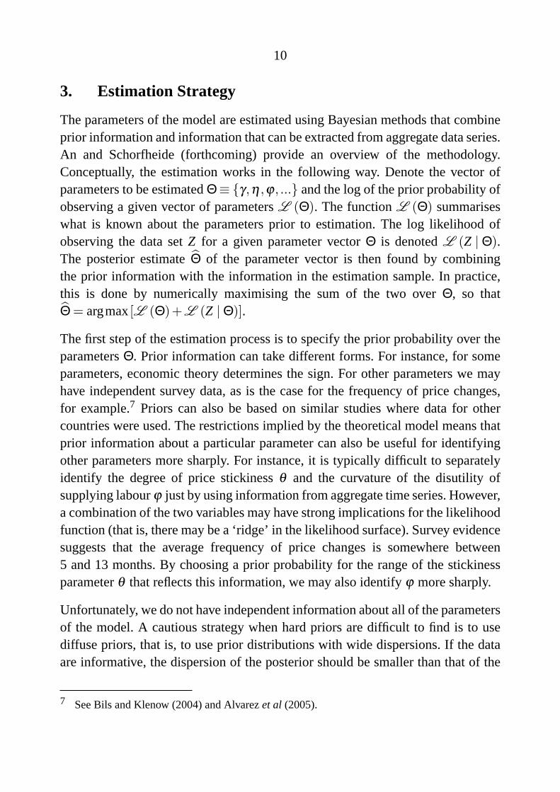
3. Estimation Strategy

The parameters of the model are estimated using Bayesian methods that combineprior information and information that can be extracted from aggregate data series.An and Schorfheide (forthcoming) provide an overview of the methodology.Conceptually, the estimation works in the following way. Denote the vector ofparameters to be estimatedΘ≡ γ,η ,ϕ, ... and the log of the prior probability ofobserving a given vector of parametersL (Θ). The functionL (Θ) summariseswhat is known about the parameters prior to estimation. The log likelihood ofobserving the data setZ for a given parameter vectorΘ is denotedL (Z | Θ).The posterior estimateΘ of the parameter vector is then found by combiningthe prior information with the information in the estimation sample. In practice,this is done by numerically maximising the sum of the two overΘ, so thatΘ = argmax[L (Θ)+L (Z | Θ)].

The first step of the estimation process is to specify the prior probability over theparametersΘ. Prior information can take different forms. For instance, for someparameters, economic theory determines the sign. For other parameters we mayhave independent survey data, as is the case for the frequency of price changes,for example.7 Priors can also be based on similar studies where data for othercountries were used. The restrictions implied by the theoretical model means thatprior information about a particular parameter can also be useful for identifyingother parameters more sharply. For instance, it is typically difficult to separatelyidentify the degree of price stickinessθ and the curvature of the disutility ofsupplying labourϕ just by using information from aggregate time series. However,a combination of the two variables may have strong implications for the likelihoodfunction (that is, there may be a ‘ridge’ in the likelihood surface). Survey evidencesuggests that the average frequency of price changes is somewhere between5 and 13 months. By choosing a prior probability for the range of the stickinessparameterθ that reflects this information, we may also identifyϕ more sharply.

Unfortunately, we do not have independent information about all of the parametersof the model. A cautious strategy when hard priors are difficult to find is to usediffuse priors, that is, to use prior distributions with wide dispersions. If the dataare informative, the dispersion of the posterior should be smaller than that of the

7 See Bils and Klenow (2004) and Alvarezet al (2005).

11

prior. However, Fukacet al (2006) point out that using informative priors, evenwith wide dispersions, can affect the posteriors in non-obvious ways.

Arguably, hard prior information exists for the discount factorβ , the steady stateshare of imports/exports in GDPα and the average duration of good pricesθ

d andθ

m. The first two can be deduced from the average real interest rate and the averageshare of imports and exports of GDP and are calibrated asβ ,α= 0.99,0.18.Calibration can be viewed as a very tight prior. The price stickiness parametersθ

d

andθm are assigned priors that are centered around the mean duration found in

European data (see Alvarezet al2005).

The prior distributions of the variances of the exogenous shocks are truncateduniform over the interval[0,∞). It is common to use more restrictive priorsfor the exogenous shocks, as for example in Smets and Wouters (2003),Lubik and Schorfheide (forthcoming), Justiniano and Preston (2005) and Kam,Lees and Liu (2006), but since most shocks are defined by the particular modelused, it is unclear what the source of the prior information would be.

The priors of the variances of the measurement error parameters are uniformdistributions on the interval[0,σ2

Zn) whereσ2Zn is the variance of the corresponding

time series. Economic theory dictates the domains of the rest of the priors, butwe have little information about their modes and dispersions. These priors aretherefore assigned wide dispersions. Information about the prior distributions forthe individual parameters are given in Table 1.

3.1 Mapping the Model into Observable Time Series

The model of Section 2 is solved by first taking linear approximations ofthe structural equations around the steady state and then finding the rationalexpectations equilibrium law of motion. The linearised equations are listed in theAppendix and the Soderlind (1999) algorithm was used to solve the model. Thesolution can be written in VAR(1) form

Xt = AXt−1+Cεt . (33)

whereXt is a vector containing the variables of the model, and the coefficientmatricesA andC are functions of the structural parametersΘ. Equation (33) iscalled thetransition equation. The next step is to decide which (combinations) of

12

Table 1: Prior and Posterior Distributions of ParametersParameter Distribution Prior Posterior

Mode Standard error Mode Standard error

Households and firms

γ normal 3 0.44 3.37 0.36

η normal 2 0.66 1.20 0.15

ϕ normal 2 0.44 1.89 0.43

ω beta 0.3 0.10 0.73 0.06

δ normal 1 0.10 0.93 0.10

δx normal 1 0.10 0.02 0.01

θ beta 0.75 0.04 0.73 0.04

θm beta 0.75 0.04 0.90 0.02

ψ normal 0.01 0.02 0.10 0.02

Taylor rule

φy normal 0.5 0.25 0.02 0.01

φπ normal 1.5 0.29 0.19 0.04

φi beta 0.5 0.25 0.87 0.03

Exogenous persistence

ρa beta 0.5 0.28 0.65 0.07

ρs beta 0.5 0.28 0.07 0.01

ρpx beta 0.5 0.28 0.87 0.06

ρx beta 0.5 0.28 0.89 0.06

ρm beta 0.5 0.28 0.71 0.13

Exogenous shock variances

σ2a uniform [0,∞) 4.66×10−5 1.59×10−5

σ2v uniform [0,∞) 4.65×10−2 5.68×10−3

σ2c uniform [0,∞) 2.32×10−5 7.03×10−6

σ2π uniform [0,∞) 6.79×10−6 2.47×10−6

σ2px uniform [0,∞) 5.32×10−5 1.74×10−5

σ2x uniform [0,∞) 7.63×10−4 6.38×10−4

σ2m uniform [0,∞) 1.34×10−5 4.44×10−6

σ2i uniform [0,∞) 7.20×10−7 1.85×10−7

13

the variables inXt are observable. The mapping from the transition equation toobservable time series is determined by themeasurement equation

Zt = DXt +et (34)

The selector matrixD maps the theoretical variables in the state vectorXt into avector of observable variablesZt . The termet is a vector of measurement errors.For theoretical variables that have clear counterparts in observable time series, themeasurement errors capture noise in the data-collecting process. The measurementerrors may also capture discrepancies between the theoretical concepts of themodel and observable time series. For instance, GDP, non-farm GDP and marketsector GDP all measure output, but none of these measures correspond exactly tothe model’s variableYt . The measure of total GDP includes farm output, whichvaries due to factors other than technology and labour inputs, most notably theweather. One may therefore want to exclude farm products. But in the model,more abundant farm goods will lead to higher overall consumption and lowermarginal utility, and perhaps also higher exports, so excluding it altogether isalso not appropriate. Total GDP also includes government expenditure which isnot determined by the utility maximising agents of the model, but it will affectthe aggregate demand for labour and therefore market wages. The state spacesystem, that is, the transition Equation (33) and the measurement Equation (34),is quite flexible and can incorporate all three measures of GDP, allowing the datato determine how well each of them corresponds to the model’s concept of output.This multiple indicator approach was proposed by Boivin and Giannoni (2005)who argue that not only does this allow us to be agnostic about which data to use,but by using a larger information set it may also improve estimation precision.

Some, but not all, of the observable time series are assumed to containmeasurement errors, and the magnitude of these are estimated together with therest of the parameters. Counting both measurement errors and the exogenousshocks, the total number of shocks in the model are more than is necessary toavoid stochastic singularity. That is, the total number of shocks are larger than thetotal number of observable variables inZt . It is reasonable to ask whether all ofthe shocks can be identified, and the answer is that it depends on the actual data-generating process. The measurement errors are white noise processes specificto the relevant time series that are uncorrelated with other indicators as well aswith their own leads and lags. To the extent that the cross-equation and dynamic

14

implications that distinguish the structural shocks from the measurement errors ofthe model are also present as observable correlations in the time series, it will bepossible to identify the structural shocks and the measurement errors separately.Incorrectly excluding the possibility of measurement errors may bias the estimatesof the parameters governing both the persistence and variances of the structuralshocks. Also, by estimating the magnitude of the measurement errors we can getan idea of how well different data series match the corresponding model concept.

3.2 Computing the Likelihood

The linearised model (33) and the measurement Equation (34) can be used tocompute the covariance matrix of the theoretical one-step-ahead forecast errorsimplied by a given parameterisation of the model. That is, without looking at anydata, we can compute what the covariance of our errors would be if the model wasthe true data-generating process and we used the model to forecast the observablevariables. This measure, denotedΩ, is a function of both the assumed functionalforms and the parameters and is given by

Ω = DPD′+Eete′t (35)

whereP is the covariance matrix of the one-period-ahead forecast errors of thestate

P = A(P−PD′(DPD′+Eete′t)−1DP)A′+CEεtε

′tC

′ (36)

The covariance of the theoretical forecast errorsΩ is used to evaluate thelikelihood of observing the time series in the sample, given a particularparameterisation of the model. Formally, the log likelihood of observingZ giventhe parameter vectorΘ is

L (Z | Θ) =−.5T∑

t=0

[pln(2π)+ ln |Ω|+u′tΩ

−1ut

](37)

wherep×T are the dimensions of the observable time seriesZ andut is a vectorof the actual one-step-ahead forecast errors from predicting the variables in thesampleZ using the model parameterised byθ . The actual (sample) one-step-aheadforecast errors can be computed from the innovation representation

Xt+1 = AXt +Kut (38)

ut = Zt −DXt (39)

15

whereK is the Kalman gain

K = PD′(DPD′+Eete′t)−1

The method is described in detail in Hansen and Sargent (2005).

To help understand the log likelihood function intuitively, consider the case ofonly one observable variable so that bothΩ and ut are scalars. The last termin the log likelihood function (37) can then be written asu2

t /Ω, so for a givensquared erroru2

t the log likelihood increases in the variance of the model’s forecasterror variance. This term will thus make us choose parameters inθ that make theforecast errors of the model large since a given error is more likely to have comefrom a parameterisation that predicts large forecast errors. The determinant termln |Ω| (the determinant of a scalar is simply the scalar itself) counters this effect,and to maximise the complete likelihood function we need to find the parametervector Θ that yields the optimal trade-off between choosing a model that canexplain our actual forecast errors,ut , while not making the implied theoreticalforecast errors too large.

Another way to understand the likelihood function is to recognise that there are(roughly speaking) two sources contributing to the forecast errorsut , namelyshocks and incorrect parameters. The set of parametersΘ that maximise thelog likelihood function (37) are those that reduce the forecast errors caused byincorrect parameters as much as possible by matching the theoretical forecast errorvarianceΩ with the sample forecast error covarianceEutu

′t , thereby attributing all

remaining forecast errors to shocks.

3.3 The Data

The data sample is from 1991:Q1 to 2006:Q2 where the first eight observationsare used as a convergence sample for the Kalman filter. Thirteen time serieswere used as indicators for the theoretical variables of the model, which is morethan that of most other studies estimating structural small open economy models.Lubik and Schorfheide (forthcoming) estimate a small open economy model ondata for Canada, the UK, New Zealand and Australia using terms of trade as theonly observable variable relating to the open economy dimension of the model.Similarly, in Justiniano and Preston (2005) the real exchange rate between the USand Canada is the only data series relating to the open economy dimension of the

16

model. Neither of these studies use trade volumes to estimate their models. Thisis also true for Kamet al (2006), though this study uses data on imported goodsprices rather than only aggregate CPI inflation.

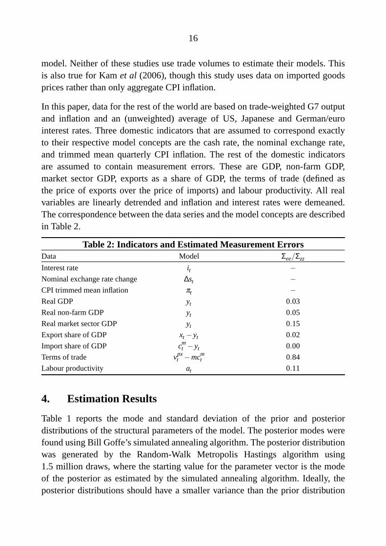
In this paper, data for the rest of the world are based on trade-weighted G7 outputand inflation and an (unweighted) average of US, Japanese and German/eurointerest rates. Three domestic indicators that are assumed to correspond exactlyto their respective model concepts are the cash rate, the nominal exchange rate,and trimmed mean quarterly CPI inflation. The rest of the domestic indicatorsare assumed to contain measurement errors. These are GDP, non-farm GDP,market sector GDP, exports as a share of GDP, the terms of trade (defined asthe price of exports over the price of imports) and labour productivity. All realvariables are linearly detrended and inflation and interest rates were demeaned.The correspondence between the data series and the model concepts are describedin Table 2.

Table 2: Indicators and Estimated Measurement ErrorsData Model Σee/Σzz

Interest rate it −Nominal exchange rate change ∆st −CPI trimmed mean inflation πt −Real GDP yt 0.03

Real non-farm GDP yt 0.05

Real market sector GDP yt 0.15

Export share of GDP xt −yt 0.02

Import share of GDP cmt −yt 0.00

Terms of trade vpxt −mcm

t 0.84

Labour productivity at 0.11

4. Estimation Results

Table 1 reports the mode and standard deviation of the prior and posteriordistributions of the structural parameters of the model. The posterior modes werefound using Bill Goffe’s simulated annealing algorithm. The posterior distributionwas generated by the Random-Walk Metropolis Hastings algorithm using1.5 million draws, where the starting value for the parameter vector is the modeof the posterior as estimated by the simulated annealing algorithm. Ideally, theposterior distributions should have a smaller variance than the prior distribution

17

since this would indicate that the data are informative about the parameters. Formost of the parameters this is the case. Two exceptions are the labour supplyelasticity ϕ and the price elasticity of consumption of imported goods,δ . Thissuggests that the values of these parameters do not have strong implications forthe dynamics of the observable time series.

The fraction of price setters whose behaviour follows a rule of thumbis estimated to be 0.73, a larger fraction than usual; see, for example,Smets and Wouters (2003), Lubik and Schorfheide (forthcoming), andJustiniano and Preston (2005). This parameter may also capture other sources ofinflation inertia, for instance from information imperfections as in Mankiw andReis (2002) and Woodford (2001). Imports seem to be more price elastic thanexports, as evidenced by the significantly larger estimated value ofδ as comparedto δ

x. The estimated frequency of price changes in the imported goods sector islower than that estimated for prices in the domestically produced goods sector.

The parameters in the Taylor rule suggest that policy responses to inflation andoutput are very gradual, with a high estimated value for the parameter on thelagged interest rate. The response of the short interest rate to output deviationsis quite small, with the short interest rate appearing to respond mostly to inflation.

4.1 Model Fit

The in-sample fit of the model can be assessed by plotting the one-period-aheadforecasts against the actual observed indicators (Figure 1).

The model provides a very good in-sample description of the dynamics of the cashrate, which is likely to be primarily because its persistence makes it easy to predict.The model is also able to fit most of the other time series reasonably well, with theexception of the terms of trade.

The variances of the errors in the measurement Equation (34) are estimatedjointly with the structural parameters of the model. These variances captureseries-specific transitory shocks to the observable time series. A low estimatedmeasurement error variance indicates that the associated observable time seriesmatches the corresponding model concept closely. The ratios of the measurementerrors over the variance of the corresponding time series are reported in Table 2.

18

Figure 1: Actual and Model’s One-period-ahead Forecasts

-0.3

0.0

0.3

–– Actual–– Model

2006

-0.1

0.0

0.1

-0.1

0.0

0.1

-0.3

0.0

0.3

-0.3

0.0

0.3

-0.2

-0.1

0.0

0.1

-0.2

-0.1

0.0

0.1

-0.02

0.00

0.02

-0.02

0.00

0.02

-0.02

0.00

0.02

-0.02

0.00

0.02

-0.02

0.00

0.02

-0.02

0.00

0.02

-0.02

0.00

0.02

-0.02

0.00

0.02

-0.06

-0.03

0.00

0.03

-0.06

-0.03

0.00

0.03

Import share of GDP

Cash rate Inflation

GDP Non-farm GDP

Export share of GDP

Nominal exchange ratedepreciation

Terms of trade

Labour productivity 20001994

200620001994

The variance ratios for the various measures of GDP are particularly interesting,since we used multiple indicators for this variable. The estimated values of theseratios indicate that real GDP appears to conform slightly better to the dynamic-and cross-equation implications of the model than real non-farm GDP, but thedifference is small. The third indicator for output – domestic market sectorGDP – appears to provide the poorest fit.

The terms of trade again stands out as the time series that the model has the biggestproblem fitting; the variance of the terms of trade is estimated to be almost entirelydue to measurement errors.

19

4.2 The Open Economy Dimension of the Model

Table 3 below reports the variance decomposition8 of the model evaluated at theestimated posterior modes reported in Table 1. The first row contains the fractionof the variances that originate from outside Australia. Foreign shocks explain65 per cent, 67 per cent and 58 per cent respectively of the variance of domesticoutput, inflation and interest rates. If, instead, a reduced-form VAR(4) in world anddomestic output, inflation and interest rates is estimated (with the world variablesassumed to be exogenous to the domestic variables), the results suggest thatforeign shocks are responsible for 49 per cent, 32 per cent and 45 per cent of thedomestic variance of output, inflation and interest rates respectively. The structuralmodel parameterised at the posterior mode thus attributesmoreof the variance ofdomestic variables to foreign shocks than the reduced-form regressions; althoughfor output and inflation, the 95 per cent probability intervals include the estimatesfrom the VAR(4).

The fact that the model can match the reduced-form evidence of the influence offoreign shocks on the Australian economy is reassuring, but is at odds with someprevious studies. Justiniano and Preston (2005), using Canadian and US data, findthat reduced-form estimates imply that a sizable fraction of domestic volatilitydoes indeed originate abroad. However, their structural model attributes less than1 per cent to foreign sources. They interpret this as a failure of their structuralmodel to capture the open economy aspects of the data, in spite of its ability toreplicate the cross-correlations and dynamics of the Canadian variables.

Apart from the fact that the models are estimated using data for different countries,what can explain this difference in results? One reason may be that Justiano andPreston let the US proxy for the world economy while in this paper the rest of theworld is represented by trade-weighted data on a larger set of countries. Any shockthat emanates from outside the US, for instance, from Europe, will be attributed

8 The variance decomposition is for the model variables, not the observable time series. For timeseries that are estimated to contain only a small measurement error component, the numbersin Table 3 are also a relatively accurate approximation to the variance decomposition of theobserved times series.

20

Table 3: Variance DecompositionShock/variable Output Inflation Exports ∆ Exchange Interest

rate rate

y π x ∆s i

Foreign ε∗t 0.65 0.67 0.97 0.88 0.58

(0.44–0.80) (0.38–78) (0.85–1) (0.76–0.95) (0.46–0.91)

Productivity εa 0.01 0.01 0 0 0

(0–0.16) (0–0.11) (0–0) (0–0.01) (0–0.01)

UIP risk εv 0 0 0 0.01 0.01

premium (0–0) (0–0) (0–0) (0.01–0.01) (0–0)

Demand εy 0.04 0 0 0 0

(0.01–0.19) (0–0.01) (0–0) (0–0) (0–0.01)

Cost push επ 0.06 0.07 0 0 0.04

(0.02–0.15) (0.04–0.22) (0–0) (0–0) (0.02–0.10)

Export price εpx 0.01 0.01 0 0.01 0

(0.01–0.05) (0–0.04) (0–0.01) (0–0.01) (0–0.03)

Export εx 0.21 0.23 0.03 0.10 0.24

demand (0.07–0.33) (0.12–0.42) (0.02–0.14) (0.07–0.16) (0.11–0.43)

Import εm 0 0 0 0 0

demand (0–0) (0–0) (0–0) (0–0) (0–0)

Taylor rule εi 0.01 0.01 0 0 0.02

(0–0.04) (0–0.03) (0–0) (0–0) (0.01–0.07)

Note: Figures in brackets indicate 95 per cent posterior probability intervals.

to the US in their reduced-form exercise, but it is not clear that a European shockwill be appropriately captured by the bilateral US-Canada data.

Another reason why the present model may better capture the impact of foreignshocks is that it is estimated using data on trade volumes. Not using data onimports and exports makes it harder for any model to distinguish between domesticdemand shocks and demand for the domestically produced goods coming fromabroad.

Table 3 also shows that the model can explain almost all of the nominal exchangerate variance endogenously. The exogenous UIP risk premium shock accounts for

21

only about 1 per cent of the variance of the nominal exchange rate and there is thusless of an exchange rate disconnect puzzle than is found by most other studies.9

These results are not significantly affected by the inclusion of measurement errorsin some of the time series. Re-estimating the model without measurement errorsdoes increase the posterior mode estimate of the variance of the nominal exchangerate attributable to risk premium shocks, but only to 4 per cent, which is still amuch lower figure than that of other studies. Also, the fraction of output varianceattributable to foreign shocks falls to 55 per cent and the variance of the interestrate attributable to foreign sources falls to 36 per cent and is thus closer to thereduced-form evidence than the estimated values when measurement errors areincluded. The fraction of domestic inflation variance attributable to foreign sourcesincreases to over 80 per cent without measurement errors.10

The importance of exogenous export demand and income shocks for the dynamicsof the model can also be gauged from Table 3. The exogenous export demandshock appears to be more important for explaining output, inflation, the exchangerate and the interest rate than for explaining the variance of exports, which mayseem odd at first glance. A possible explanation for this could be that whenincreased export demand is driven by world developments (which dominates thevariance decomposition for exports), imports increase and production for domesticconsumption falls. The exogenous demand shock could then be the component ofexport demand that is not associated with a similar switch of production away fromdomestic consumption goods. This would lead to the exogenous export demandshock being important for the variance of domestic output, but not very importantfor the overall variance of exports.

9 The literature on the exchange rate disconnect puzzle is very large. The seminal paper thatdefined the ‘puzzle’ is Meese and Rogoff (1983), who showed that exchange rates are veryvolatile and appear to be disconnected from the macro fundamentals. Examples of recentpapers that find a much larger role for the UIP shock are Lubik and Schorfheide (2005) andLindeet al (2004).

10 The model without measurement errors was estimated using real GDP as the only indicator fordomestic output. More details of the model estimates without measurement errors are availablefrom the author upon request.

22

4.3 The Impact of a Monetary Policy Shock

Figure 2 below displays the impulse responses to a unit shock to the (annualised)cash rate for selected endogenous variables together with the 95 per cent highestmarginal likelihood intervals.

Figure 2: Monetary Policy Shock

0.0

0.4

0.8

–– Posterior mean–– 95 per cent posterior

probability intervals

-0.5

0.0

0.5

-0.5

0.0

0.5

-2

-1

0

-2

-1

0

-0.8

-0.4

0.0

0.4

-0.8

-0.4

0.0

0.4

-2

0

2

-2

0

2

-2

0

2

-2

0

2

-0.4

0.0

-0.4

0.0

-0.4

0.0

-0.4

0.0

-15

-10

-5

0

-15

-10

-5

0

Consumption

Cash rate GDP

Inflation Exports

Consumption imports

Relative price of imports Domestic inflation

Nominal depreciation

2419144 9

2419144 9

An unanticipated increase in interest rates leads to a fall in output with themaximum negative response of 1.3 percentage points occurring after threequarters. There are two factors contributing to the fall in output. First, thehigher real interest rate leads to a fall in domestic consumption. Second, thehigher return on domestic bonds leads to a higher demand for the domesticcurrency denominated assets, leading to a currency appreciation. Lower domestic

23

consumption and less demand for labour both reduce the market real wage,causing a fall in inflation. This is reinforced by the appreciating exchange ratewhich makes imports cheaper and further decreases inflation. (However, initiallyconsumer prices of imported goods do not fall as much as domestically producedgoods, which makes imported goods initially relatively more expensive.) Thepeak response of (annualised) inflation to the unit shock to the interest rate isa fall of approximately 0.4 percentage points three quarters after impact. Theestimated maximum response of output and inflation to a monetary policy shockis faster than that which is found in some other studies, including those employingSVARs.11 Some of this difference may be explained by the relatively stringentrestrictions imposed by the structural model compared to an SVAR. Another factorthat could contribute to the relatively rapid response to a monetary policy shockin the present model may be that the sample used does not include the changeto an inflation-targeting regime in the early 1990s. If the credibility of the newmonetary policy regime was established only gradually, then this could contributeto relatively slow estimated responses of inflation and output to an increase in thecash rate for studies that incorporate this transitory period.

4.4 The Impact of Export Demand and Income Shocks

The effects of an exogenous increase in the demand for Australian exports areillustrated in Figure 3. A 1 percentage point increase in export demand leads onimpact to a 0.2 percentage point increase in GDP (consistent with the share ofthe export sector in GDP). It also leads to an appreciation of the exchange rate andboosts imports. The appreciating exchange rate leads to a fall in inflation, though itis quantitatively small (less than 0.03 percentage points at the maximum impact).These effects can be contrasted with the estimated response to a positive shockto the export price. Remember, the main difference between the export price anddemand shock is that a price shock does not put direct pressure on the domesticlabour market. Figure 4 shows that an income shock, like a demand shock, leadsto an appreciation of the exchange rate. The response of the endogenous variablesare very similar, with the exception of the volume of exports, which falls due tothe appreciating exchange rate. Due to the low elasticity of export demand, thequantitative effect is small.

11 See for instance Dungey and Pagan (2000) and Berkelmans (2005).

24

Figure 3: Export Demand Shock

-0.04

0.00

–– Posterior mean–– 95 per cent posterior

probability intervals

-0.3

0.0

-0.3

0.0

0.0

0.2

0.0

0.2

-0.08

-0.04

0.00

-0.08

-0.04

0.00

0.0

0.4

0.8

0.0

0.4

0.8

0.0

0.2

0.4

0.0

0.2

0.4

-0.04

0.00

-0.04

0.00

0.0

0.5

0.0

0.5

-3

-2

-1

0

-3

-2

-1

0

Consumption

Cash rate GDP

Inflation Exports

Consumption imports

Relative price of imports Domestic inflation

Nominal depreciation

2520105 15

2520105 15

25

Figure 4: Export Income Shock

-0.04

0.00

–– Posterior mean–– 95 per cent posterior

probability intervals

-0.3

0.0

-0.3

0.0

0.0

0.2

0.0

0.2

-0.08

-0.04

0.00

-0.08

-0.04

0.00

0.0

0.4

0.8

0.0

0.4

0.8

0.0

0.2

0.4

0.0

0.2

0.4

-0.08

-0.04

0.00

-0.08

-0.04

0.00

-0.08

-0.04

0.00

-0.08

-0.04

0.00

-3

-2

-1

0

-3

-2

-1

0

Consumption

Cash rate GDP

Inflation Exports

Consumption imports

Relative price of imports Domestic inflation

Nominal depreciation

2419144 9

2419144 9

26

4.5 The Impact of a Productivity Shock

Figure 5 plots the impulse responses to a unit shock to Australian productivity. Asexpected, GDP increases, inflation falls and the nominal exchange rate appreciates.A less obvious effect is that the consumption of imported goods falls in spite of theappreciating exchange rate. This is because domestic goods prices fall sufficientlyso as to make imports relatively more expensive.

Figure 5: Productivity Shock

-0.04

0.00

–– Posterior mean–– 95 per cent posterior

probability intervals

0.0

0.2

0.4

0.0

0.2

0.4

0.0

0.2

0.0

0.2

-0.2

-0.1

0.0

0.1

-0.2

-0.1

0.0

0.1

-0.15

0.00

0.15

-0.15

0.00

0.15

0.0

0.1

0.2

0.0

0.1

0.2

-0.10

-0.05

0.00

-0.10

-0.05

0.00

-0.02

-0.01

0.00

-0.02

-0.01

0.00

-1.0

-0.5

0.0

-1.0

-0.5

0.0

Consumption

Cash rate GDP

Inflation Exports

Consumption imports

Relative price of imports Domestic inflation

Nominal depreciation

2419144 9

2419144 9

27

5. Conclusion

This paper presents a small structural model of the Australian economy estimatedusing Bayesian techniques and based on a standard New Keynesian small openeconomy specification similar to that used by numerous other studies. However,there are four aspects in which the estimation of the model deviates from previousstudies.

The first is that the export demand and export income equations are amended withexogenous shocks to control for the prominent role played by commodities inthe Australian export sector. When the model is estimated, the export demandshock appears to play a larger role than the export income shock in explaining thevariance of domestic variables.

Second, a larger number of time series were used to estimate the model. Inparticular, data on import and export volumes were used in addition to the standardaggregate variables to ensure that the data span the open economy dimension ofthe model.

Third, flat prior distributions were used for the variances of the structural shocks.This reflects the fact that most of the structural shocks are defined jointly by themodel and the data with little or no role for economic theory nor independentsources of information to help determine the magnitude of these shocks.

Fourth, the magnitude of measurement errors in some of the time series wereestimated together with the structural parameters of the model. This acknowledgesthe fact that not only is error sometimes introduced through the data collectionprocess, but also that the model variables do not always have clear-cut counterpartsin observable time series.

The estimated model provides a good fit for most of the observable variablesand appears to be able to capture the open economy dimensions of the datareasonably well. The model can match the evidence from reduced-form studieson the importance of foreign shocks to the domestic variance of output, inflationand interest rates. The model also relies much less than other estimated structuralmodels on a persistent UIP risk premium shock to explain movements in thenominal exchange rate. Given the simplicity of the model, these results holdpromise for the usefulness of these types of open economy models as analyticaltools. However, there are other dimensions in which the model performs less well.

28

Particularly, movements in the terms of trade are not well captured by the modeland the reasons for this should be a subject of future investigation.

29

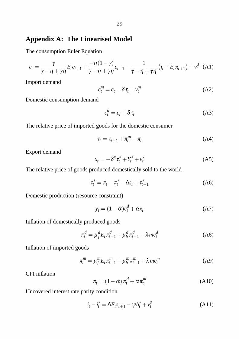
Appendix A: The Linearised Model

The consumption Euler Equation

ct =γ

γ −η + γηEtct+1+

−η(1− γ)γ −η + γη

ct−1−1

γ −η + γη

(it −Etπt+1

)+vd

t (A1)

Import demandcm

t = ct −δτt +vmt (A2)

Domestic consumption demand

cdt = ct +δτt (A3)

The relative price of imported goods for the domestic consumer

τt = τt−1+πmt −πt (A4)

Export demandxt =−δ

xτ∗t +Y∗

t +vxt (A5)

The relative price of goods produced domestically sold to the world

τ∗t = πt −π

∗t −∆st + τ

∗t−1 (A6)

Domestic production (resource constraint)

yt = (1−α)cdt +αxt (A7)

Inflation of domestically produced goods

πdt = µ

df Etπ

dt+1+ µ

dbπ

dt−1+λmcdt (A8)

Inflation of imported goods

πmt = µ

mf Etπ

mt+1+ µ

mb π

mt−1+λmcmt (A9)

CPI inflationπt = (1−α)π

dt +απ

mt (A10)

Uncovered interest rate parity condition

it − i∗t = ∆Etst+1−ψb∗t +vst (A11)

30

Flow budget constraint

b∗t+1 = b∗t +xt −cmt +vpx

t +∆st (A12)

Labour supply decision

wt − pt − γ(ct −ηct−1

)= ϕnt (A13)

wt − pt = ϕ (yt −at)+ γ(ct −ηct−1

)(A14)

Real domestic marginal cost (the real wage divided by marginal productivity oflabour)

mct = γ(ct −ηct−1

)+ϕnt −at (A15)

ormct = γct − γηct−1+ϕyt − (ϕ +1)at (A16)

Real marginal cost of imported goods

mcmt = st + pwt − pt (A17)

ormcmt = ∆st +π

wt −πt +mcmt−1 (A18)

The Taylor rule describing monetary policy

it = φyyt−1+φππt−1+φi it−1+ εit (A19)

31

References

Alvarez LJ, E Dhyne, MM Hoeberichts, C Kwapil, H Le Bihan, P L unneman,F Martins, R Sabbatini, H Stahl, P Vermeulen and J Vilmunen (2005),‘StickyPrices in the Euro Area: A Summary of New Micro Evidence’, European CentralBank Working Paper Series No 563.

An S and F Schorfheide (forthcoming),‘Bayesian Analysis of DSGE Models’,Econometric Review.

Bacchetta P and E van Wincoop (2006),‘Can Information HeterogeneityExplain the Exchange Rate Determination Puzzle?’,American Economic Review,96(3), pp 552–576.

Benigno P (2001),‘Price Stability with Imperfect Financial Integration’, Centrefor Economic Policy Research Working Paper No 2854.

Berkelmans L (2005), ‘Credit and Monetary Policy: An Australian SVAR’,Reserve Bank of Australia Research Discussion Paper No 2005-06.

Bils M and PJ Klenow (2004), ‘Some Evidence on the Importance of StickyPrices’,Journal of Political Economy, 112(5), pp 947–985.

Boivin J and M Giannoni (2005), ‘DSGE Models in a Data-Rich Environment’,Columbia University, unpublished manuscript.

Calvo GA (1983), ‘Staggered Prices in a Utility-Maximizing Framework’,Journal of Monetary Economics, 12(3), pp 383–398.

Corsetti G and P Pesenti (2005),‘The Simple Geometry of Transmission andStabilization in Closed and Open Economies’, NBER Working Paper No 11341.

Department of Foreign Affairs and Trade (2005), Composition of Trade,available at<http://www.dfat.gov.au/publications/>.

Dungey M and A Pagan (2000),‘A Structural VAR Model of the AustralianEconomy’,The Economic Record, 76(235), pp 321–342.

Fukac M, A Pagan and V Pavlov (2006),‘Econometric Issues Arising fromDSGE Models’, Australian National University, unpublished manuscript.

32

Galı J and M Gertler (1999), ‘Inflation Dynamics: A Structural EconometricAnalysis’,Journal of Monetary Economics, 44(2), pp 195–222.

Galı J and T Monacelli (2005),‘Monetary Policy and Exchange Rate Volatilityin a Small Open Economy’,Review of Economic Studies, 72(3), pp 707–734.

Hansen L and T Sargent (2005),‘Recursive Methods for Linear Economies’,University of Chicago and New York University.

Justiniano A and B Preston (2005),‘Can Structural Small Open EconomyModels Account for the Influence of Foreign Disturbances?’, ColumbiaUniversity, unpublished manuscript.

Kam T, K Lees and P Liu (2006), ‘Uncovering the Hit-List for Small InflationTargeters: A Bayesian Structural Analysis’, Reserve Bank of New ZealandDiscussion Paper No DP2006/09.

Lind e J, M Nessen and U Soderstrom (2004), ‘Monetary Policy in anEstimated Open-Economy Model with Imperfect Pass-Through’, SverigesRiksbank Working Paper Series No 167.

Lubik T and F Schorfheide (2005),‘A Bayesian Look at New Open EconomyMacroeconomics’, John Hopkins University, Department of Economics WorkingPaper No 521.

Lubik T and F Schorfheide (forthcoming), ‘Do Central Banks Respond toExchange Rate Movements? A Structural Investigation’,Journal of MonetaryEconomics.

Mankiw G and R Reis (2002), ‘Sticky Information Versus Sticky Prices: AProposal to Replace the New Keynesian Phillips Curve’,Quarterly Journal ofEconomics, 117(4), pp 1295–1328.

Meese RA and K Rogoff (1983),‘Empirical Exchange Rate Models of theSeventies: Do they Fit Out of Sample?’,Journal of International Economics,14(1–2), pp 3–24.

Nessen M (2006), ‘How are DSGE Models Used in Policy-Making?’, paperpresented at a workshop on ‘The Interface between Monetary Policy and MacroModelling’, Reserve Bank of New Zealand, Wellington, 13–15 March.

33

Smets F and R Wouters (2003),‘An Estimated Stochastic General EquilibriumModel of the Euro Area’,Journal of the European Economic Association, 1(5),pp 1123–1175.

Smets F and R Wouters (2004),‘Forecasting with a Bayesian DSGE Model:An Application to the Euro Area’,Journal of Common Market Studies, 42(4),pp 841–867.

Soderlind P (1999),‘Solution and Estimation of RE Macromodels with OptimalPolicy’, European Economic Review, 43(4–6), pp 813–823.

Woodford M (2001), ‘Imperfect Common Knowledge and the Effects ofMonetary Policy’, NBER Working Paper No 8673.