research discussion paper - reserve bank … bank of australia reserve bank of australia economic...
TRANSCRIPT

Reserve Bank of Australia
Reserve Bank of AustraliaEconomic Research Department
2011
-05
RESEARCHDISCUSSIONPAPER
Terms of Trade Shocks: What are Th ey and What Do Th ey Do?
Jarkko Jääskelä and Penelope Smith
RDP 2011-05

TERMS OF TRADE SHOCKS: WHAT ARE THEY ANDWHAT DO THEY DO?
Jarkko Jaaskela and Penelope Smith
Research Discussion Paper2011-05
December 2011
Economic Research DepartmentReserve Bank of Australia
We would like to thank Jonathan Kearns, Adrian Pagan and participantsof the 2011 Australasian Meeting of the Econometric Society in Adelaide.Responsibility for any remaining errors rests with us. The views expressed in thispaper are those of the authors and are not necessarily those of the Reserve Bankof Australia.
Authors: jaaskelaj and smithp at domain rba.gov.au
Media Office: [email protected]

Abstract
This paper describes and quantifies the macroeconomic effects of different typesof terms of trade shocks and their propagation in the Australian economy. Threetypes of shocks are identified based on their impact on commodity prices, globalmanufactured prices, and global economic activity. The first two shocks, a worlddemand shock and a commodity-market specific shock are fairly standard. Thethird shock, a globalisation shock that may result, for instance, from the increasingimportance of China, India and eastern Europe in the global economy is morenovel. The globalisation shock is associated with a decline in manufactured prices,a rise in commodity prices, and an increase in global economic activity.
Determining the underlying source of variation in the terms of trade is shown tobe important for understanding the impact on the Australian economy as all threeshocks propagate through the economy in different ways. The relative contributionof each shock to inflation, output, interest rates, and the exchange rate has alsovaried over time. The main conclusion of the paper is that a higher terms of tradetends to be expansionary but is not always inflationary. A key result is that thefloating exchange rate has provided an important buffer to the external shocks thatmove the terms of trade.
JEL Classification Numbers: E32, E52, F36, F40Keywords: terms of trade, sign-restricted VAR
i

Table of Contents
1. Introduction 1
2. Measuring the Effects of Terms of Trade Shocks 3
2.1 The Benchmark VAR 5
2.2 Identification Using Sign and Parametric Restrictions 6
3. Results 8
3.1 Impulse Responses 8
3.2 Variance Decomposition 11
3.3 Historical Decomposition 13
3.4 Additional Results and Robustness Checks 173.4.1 Estimation over the inflation-targeting period 173.4.2 Direct versus indirect effects on inflation 18
4. Conclusion 20
Appendix A: Data Description and Sources 22
Appendix B: Robustness Checks 23
References 31
ii
TERMS OF TRADE SHOCKS: WHAT ARE THEY ANDWHAT DO THEY DO?
Jarkko Jaaskela and Penelope Smith
1. Introduction
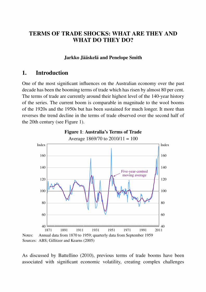
One of the most significant influences on the Australian economy over the pastdecade has been the booming terms of trade which has risen by almost 80 per cent.The terms of trade are currently around their highest level of the 140-year historyof the series. The current boom is comparable in magnitude to the wool boomsof the 1920s and the 1950s but has been sustained for much longer. It more thanreverses the trend decline in the terms of trade observed over the second half ofthe 20th century (see Figure 1).
Figure 1: Australia’s Terms of TradeAverage 1869/70 to 2010/11 = 100
40
60
80
100
120
140
160
40
60
80
100
120
140
160
Five-year-centredmoving average
2011
IndexIndex
1991197119511931191118911871Notes: Annual data from 1870 to 1959; quarterly data from September 1959Sources: ABS; Gillitzer and Kearns (2005)
As discussed by Battellino (2010), previous terms of trade booms have beenassociated with significant economic volatility, creating complex challenges

2
for economic policy. The booms of the 1920s and 1950s, although initiallyexpansionary, were followed by falling output and rising unemployment. With afixed exchange rate in place during the 1950s, the concurrent rise in export receiptsand capital inflows caused a surge in money and credit, resulting in year-ended CPIinflation of almost 20 per cent. In the period since the float of the Australian dollarthe exchange rate response to a change in the terms of trade has become central tothe macroeconomic outcome. Gruen and Shuetrim (1994) found evidence that, inthe period after the float of the Australian dollar, rises in the terms of trade havetended to reduce domestic inflation in the short run.
We argue that the consequences of a rising terms of trade will ultimately dependon the characteristics of the underlying shock, as well as the policy response. Inrelated work, Kilian (2009) and Peersman and Van Robays (2009) demonstratethat the responses of the US and euro area economies to oil price shocks alsodepend on the nature of the shock. The recent Australian empirical literature,however, largely ignores this idea.
We identify the impact of global shocks on the terms of trade by estimating asign-restricted vector autoregression (VAR). Three stylised terms of trade shocksare identified: a world demand shock, a commodity-market specific shock, and aglobalisation shock. A positive world demand shock is associated with a pick-upin global economic activity and an increase in export and import prices. A positivecommodity-market specific shock increases export prices without a correspondingpick-up in global economic activity.
Finally, a globalisation shock captures the increasing integration of emergingeconomies, notably China and India, into the world economy. Increasedglobalisation has been associated with a fall in the relative price of manufacturedgoods. As Australian imports are concentrated in manufactured goods this is alsolikely to increase the terms of trade. At the same time, as more countries integratein to the world economy, the demand for raw materials increases, exerting upwardpressure on (commodity) export prices. Such a shock is also associated with anexpansion in world output.
We find that positive terms of trade shocks tend to be expansionary but are notalways inflationary. Whether these shocks are inflationary depends on both thesource of the shock and the response of monetary policy. We also find that thefloating exchange rate provides an important buffer against foreign shocks that

3
move the terms of trade: the bulk of variation in the real exchange rate is attributedto world shocks, but the world shocks have very little impact on other Australianvariables.
The remainder of the paper is structured as follows. In Section 2 we outline ourbenchmark VAR and discuss identification of the shocks that move the terms oftrade. In Section 3 we estimate the effects of these shocks on Australian inflation,output, short-term nominal interest rates, and the real exchange rate. We alsoobtain the historical contribution of each identified shock to fluctuations in thedomestic variables. The concluding remarks are in Section 4.
2. Measuring the Effects of Terms of Trade Shocks
A standard framework for estimating the effects of international relative priceshocks on the Australian economy is to estimate a VAR model that is partitionedinto an exogenous foreign block, designed to capture conditions in the worldeconomy, and a domestic block that includes output, inflation, interest rates, andthe real exchange rate. Movements in international relative prices are captured inseveral different ways. Berkelmans (2005) and Lawson and Rees (2008) includereal commodity prices, while in Dungey and Pagan (2000, 2009) and Otto (2003)the terms of trade are included. Brischetto and Voss (1999) include world oilprices. This international relative price variable is typically included in the worldblock.
To capture fluctuations in international relative prices that are not explained bymovements in world output or world interest rates, a shock is typically applieddirectly to the relative price variable. The implication of this approach is that allrelative price shocks are treated equally. For example, a rise in the terms of tradeassociated with a fall in the price of manufactured goods is assumed to have similarconsequences for the Australian economy as a rise in the terms of trade associatedwith higher world commodity prices and higher world manufactures prices.
We also adopt a VAR framework, but depart from the standard approach inallowing the response of domestic variables to vary depending on the natureof the terms of trade shock. Liu (2010) also examines the effect of differenttypes of international shocks on the Australian economy but like Dungey andPagan (2000, 2009), Liu assumes that terms of trade shocks do not influenceforeign variables. In contrast, we maintain the small open economy assumption

4
that the prices of tradeable goods are determined in world markets, implying thatall terms of trade shocks originate in (and affect) the world economy.
Before outlining our identification scheme, it is helpful to briefly review the keyinfluences on Australia’s terms of trade over recent years. These include the globalbusiness cycle, the rapid development of Asian economies, and the sticky responseof supply in commodities markets.
As discussed by Kilian (2009), there is little direct evidence of how the globalbusiness cycle affects industrial commodity markets, although there is typicallya positive correlation between global output growth and commodity prices. Forexample, the 2000s boom in global commodity prices was associated with strongeconomic growth worldwide, particularly in Asia. The long time horizons ofcapital-intensive investment in the mining sector meant supply could not quicklyexpand to meet unexpected changes to demand and commodity prices rose sharply(see Connolly and Orsmond (2011)).
Strong growth in commodity prices in recent years has also been linked to theunusually high, and rising, intensity of use of metals in industrialising Asia. In2007, GDP metal intensities in China were 7.5 times higher than in developedcountries and 4 times higher than in other developing countries (IBRD/WorldBank 2009). This reflects the resource intensity of the infrastructure investmentrequired to support rural–urban migration, investment in physical capital suchas plants and infrastructure, as well as lower rates of efficiency in the useof these resources. The composition of Chinese exports also appears to havebeen important. Roberts and Rush (2010) provide evidence that China’s (mainlymanufacturing) exports have been at least as important as construction as a driverof China’s demand for resource commodities.
The sharp expansion in the supply of manufactured goods accompanying theintegration of east Asia into the world economy and the transfer of manufacturingactivities to these economies has placed downward pressure on the world priceof manufactured goods. As Australian imports are concentrated in manufacturedgoods, this is an additional factor supporting Australia’s terms of trade.

5
2.1 The Benchmark VAR
To distill the various global shocks underlying movements in the terms of tradewe estimate the following sign-restricted VAR:
[wtdt
]= αxt +
p∑i=1
Ai
[wt−idt−i
]+B
[ε
wt
εdt
](1)
where wt and dt are vectors of endogenous world and domestic variables, xt is avector of exogenous variables, and B is the contemporaneous impact matrix of thevectors of mutually uncorrelated world ε
wt and domestic ε
dt disturbances.
There are three variables in the world block wt = (πxt ,πm
t ,∆ywt )′ which broadly
capture conditions in the world economy that are exogenous to the Australianeconomy, but relevant to Australia’s terms of trade: π
xt is export price inflation;
πmt is import price inflation; and yw
t is quarterly growth in the output of Australia’smajor trading partners.1 To abstract from fluctuations in export and import pricescaused by movements in the exchange rate, the export and import price series areconverted to world prices using the trade-weighted index.2
The second group of variables dt = (∆ydt ,πd
t ,rdt ,∆qt)
′ are specific to the Australianeconomy: ∆yd
t denotes domestic output growth; πdt is consumer price inflation; rd
tis the nominal short-term interest rate; and ∆qt is the log difference of the realexchange rate. Appendix A contains a full description of the data and their sources.
The sample used for estimation runs from 1984:Q1 to 2010:Q2. It was selectedto include the earlier period of strong commodity price growth in the late 1980s.The start date is constrained by the float of the Australian dollar in December1983. In order to capture the move to inflation targeting, a constant and a dummyvariable are included in the vector xt . The dummy variable is equal to 1 during theinflation-targeting period from March 1993 onward, and 0 otherwise.
1 We also estimated the model with a measure of world industrial production but found that it didnot substantially alter the results.
2 We are assuming instantaneous and perfect pass through of the nominal exchange rate intoexport and import prices. Indices of world manufacturing or commodity prices are typicallyconstructed under this assumption.

6
Augmented Dickey-Fuller and Phillips-Perron tests indicate that all variables inthe benchmark model are I(1), except for the domestic interest rate which isI(0). Trace tests failed to find evidence of a cointegrating relationship amongstthe variables in the model and we specify the model in differences rather than inlevels. The results presented are for a lag length of p = 3.
2.2 Identification Using Sign and Parametric Restrictions
Identification of structural shocks in VAR models is typically achieved byplacing restrictions on the model parameters. However, an increasingly popularalternative is to place restrictions on the direction that key variables willmove (over a given horizon) in response to different types of shocks. VARmodels identified using this technique are known as sign-restricted VARs. Signrestrictions have been used as a method of identifying structural shocks in VARmodels by Faust (1998), Canova and De Nicolo (2002), and Uhlig (2005).Peersman and Van Robays (2009) demonstrate the use of sign restrictions inidentifying different types of oil price shocks.3
We use a combination of sign and parametric restrictions. Sign restrictions areimposed on the estimated responses of the level of export prices (px
t ), import prices(px
t ), and world output (ywt ) to identify different types of global shocks that move
Australia’s terms of trade. This amounts to placing restrictions on the signs of theaccumulated impulse responses. The specific shocks that we consider are a ‘worlddemand’ shock, a world ‘commodity-market specific’ shock, and a ‘globalisation’shock. The sign restrictions adopted in this paper are presented in Table 1. Therestrictions are imposed for four periods following a shock, as is standard in theliterature.
The interpretation of the world demand shock in Table 1 is straightforward.It captures movements in export and import prices associated with the globalbusiness cycle. A positive world demand shock increases px
t , pmt , and yw
t . Theglobalisation shock captures the integration of emerging market economies intothe world trade system, resulting in stronger world growth and higher worldcommodity prices, while at the same time placing downward pressure on theprice of manufactured goods (import prices). Finally, innovations to export prices
3 Fry and Pagan (forthcoming) provide a comprehensive review of literature on sign-restrictedVARs.

7
Table 1: VAR Restrictions on Shocks that Improve the Terms of Tradepx pm yw d
World demand shock + + + naCommodity-market specific shock + na − naGlobalisation shock + − + naDomestic shocks 0 0 0 na
Notes: + (−) means a positive (negative) response of the variable in the column to the shock in the row; 0 meansno response as implied by the small open economy assumption; na means no restriction is imposed on theresponse
that are not explained by world demand or globalisation shocks are attributed tothe commodity-market specific shock. This shock accounts for periods of risingcommodity prices that are not associated with a pick-up in world output growth.As this shock also captures financial investment in commodities and precautionarydemand, its impact on world output may be positive or negative.
Note that the restrictions used to identify the globalisation shock are the only onesthat also restrict the response of the terms of trade. However, because π
xt is more
volatile than πmt we expect that positive world demand and commodity market
specific shocks will also increase the terms of trade.
In keeping with the small open economy assumption, we restrict thecontemporaneous impact matrix B and lag matrices Ai to be block lower triangular.This implies that fluctuations in the world price of Australian exports andimports and world output are only driven by shocks to the world block (εw
t ).Even though there are seven shocks in the model, we only need to identifythe three world shocks to avoid the multiple shocks problem described by Fryand Pagan (forthcoming). Since we are mainly interested in the response of thedomestic variables to different types of foreign shocks, we do not place restrictionson the domestic variables or identify domestic shocks. A similar approach istaken by Peersman and Van Robays (2009), although they do not place parametricrestrictions on the Ai matrices.

8
3. Results
3.1 Impulse Responses
We follow Peersman (2005) in using a Bayesian approach for estimation andinference and hence capture both sampling and model uncertainty.4 A total of100 000 successful draws from the posterior are used to show the median, 84thand 16th percentiles of the impulse responses.5 Figure 2 shows the accumulatedimpulse responses of the world variables to the three identified shocks. Thedirection of these responses (for the first four periods) correspond to therestrictions outlined in Table 1. The magnitudes of these responses, however, areunrestricted. Figure 2 also shows the impulse responses for the terms of trade,which are constructed from the responses of export and import prices.
Fry and Pagan (forthcoming) criticise the practise of using the median responseas a measure of central tendency because it mixes the responses of differentcandidate models. They suggest selecting a single model, and hence the uniqueset of impulse responses from the Monte Carlo draws that is closest to the set ofmedian responses. Accordingly, we also report their ‘median target’ measure. Tolocate this measure we use the impulse responses from all seven variables in themodel.
The responses of variables in the world block to world shocks appear to bepermanent. This is consistent with pretesting which indicated that each serieswas I(1). The effect of each shock on the terms of trade also appears to bepermanent, providing additional evidence that export prices and import prices arenot cointegrated. Although the magnitudes of the responses of export and importprices to each shock are different, the response of the terms of trade is similar. Eachidentified shock permanently increases the terms of trade by around 2–4 per centaccording to the median target measure.
The response of import prices to the commodity-market specific shock is theonly unrestricted response in the world block. The response is clearly positive
4 Detailed descriptions of algorithms used for Bayesian inference in these models can be foundin Peersman (2005), Uhlig (2005), and Rubio-Ramırez, Waggoner and Zha (2010).
5 Because the point-wise distribution of each impulse response is approximately normal, the 16thand 84th percentiles roughly correspond to a one standard deviation error band.

9
Figure 2: Responses of World Variables to Terms of Trade Shocks
2
4
6
■ Percentile bands — Median — Median target
0 5 10 15 20-2
0
2
4
2
4
6
5 10 15 20-2
0
2
4
0
1
0
1
-1012
Worlddemand shock
Quarters after shock5 10 15 20
Com-mktspec shock
Globalisation shock
Expo
rt pr
ices
Impo
rt pr
ices
Wor
ld o
utpu
tTe
rms o
f tra
de
210-1
Notes: Figures show the median and median target accumulated impulse responses to thedifferent types of terms of trade shocks, together with the 16th and 84th percentilebands. The impulse responses for the terms of trade are constructed from the impulseresponses for export prices and import prices. ‘Com-mkt spec shock’ is a commodity-market specific shock.
for the first two quarters, before returning to zero. The response of world outputto the commodity-market specific shock is clearly negative. The responses toa commodity-market specific shock are consistent with a textbook ‘commoditysupply’ shock, where a disruption to the supply of commodities is followed byan increase in commodity prices, a rise in the price of goods that use thosecommodities as an input, and a fall in world output. However, without a reliablelong-run measure of the world supply of Australia’s major export commoditiessuch as coal and iron ore, it is impossible to identify a commodity supply shock.

10
Figure 3 shows the unrestricted responses of domestic variables to the shocksidentified in Table 1. The first column shows the response of the domesticvariables to a positive world demand shock. In response to this shock thereis a permanent appreciation in the real exchange rate of 2–3 per cent. Themedian impulse response suggests that level of output is 0.25 per cent higher forthree quarters, although the median target measure suggests a somewhat weakerresponse. Nominal interest rates increase by about 50 basis points and remainelevated for around two years. Inflation is slightly higher on impact (due to higherimport prices), but rapidly returns to zero as the exchange rate appreciates and theinterest rate increases.
Figure 3: Responses of Domestic Variables to Terms of Trade Shocks
0
2
4
■ Percentile bands — Median — Median target
Worlddemand shock
Quarters after shock5 10 15 20
Com-mktspec shock
Globalisation shock
Real
exch
ange
rate
Dom
estic
out
put
Infla
tion
rate
Inte
rest
rate
4
2
0
0.5
0.0
0.5
0.0
0.0
-0.1
0.0
-0.1
0 5 10 15 20
0.5
0.0
-0.5
-1.05 10 15 20
0.5
-0.5
0.0
-1.0
Notes: Figures show the median and median target impulse responses to the different types ofterms of trade shocks, together with the 16th and 84th percentile bands. The accumulatedimpulse responses are shown for output and the real exchange rate.

11
The central column of Figure 3 contains the responses to a commodity-marketspecific shock. In response to this shock, the real exchange rate appreciates byaround 3 per cent on impact and then depreciates by the same amount over the nextthree quarters. The higher real exchange rate appears to be passed through to lowerconsumer prices for three quarters after the shock, although the magnitude of theinflation response is small (less than 0.1 per cent per quarter). This suggests thatany domestic inflationary pressures that might arise from the higher import pricesare offset by the higher real exchange rate, and the interest rate falls accordingly.According to the median and median target, the level of domestic output ispermanently higher following a commodity-market specific shock, however thestrength of this response is imprecisely measured, with the 16th percentile bandtouching zero.
The last column of Figure 3 shows the response of the domestic variablesto a positive globalisation shock. In this case the real exchange rate appearsto depreciate, although the estimated magnitude of this depreciation is small.Although it may be surprising to see the real exchange rate depreciate in responseto a positive shock to commodity prices, this response is consistent with a Balassa-Samuelson type effect. Domestic inflation falls on impact before returning to trendin 4 to 8 quarters, perhaps due to the depreciation of the real exchange rate. Thereis no significant response by the short-term nominal interest rate or output.
To summarise, the evidence presented here is that terms of trade shocks are notnecessarily expansionary or inflationary, with the net effect dependent upon thenature of the underlying shock. The real exchange rate appears to have provided animportant buffer against foreign shocks over the sample period. Overall, monetarypolicy – as captured by the short-term market interest rate – has tended to respondto the foreign shocks in such a way that it reduces the inflationary effect of theseshocks.
3.2 Variance Decomposition
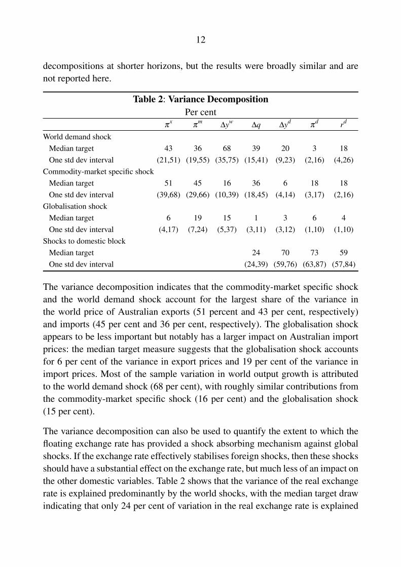
Table 2 reports the contribution of the three identified shocks to the unconditionalvariance of the data. We report the results for the median target draw, rather thanthe median because the construction of variance, and historical, decompositionsrequires that shocks come from a unique model. We also examined variance
12
decompositions at shorter horizons, but the results were broadly similar and arenot reported here.
Table 2: Variance DecompositionPer cent
πx
πm
∆yw∆q ∆yd
πd rd
World demand shockMedian target 43 36 68 39 20 3 18One std dev interval (21,51) (19,55) (35,75) (15,41) (9,23) (2,16) (4,26)
Commodity-market specific shockMedian target 51 45 16 36 6 18 18One std dev interval (39,68) (29,66) (10,39) (18,45) (4,14) (3,17) (2,16)
Globalisation shockMedian target 6 19 15 1 3 6 4One std dev interval (4,17) (7,24) (5,37) (3,11) (3,12) (1,10) (1,10)
Shocks to domestic blockMedian target 24 70 73 59One std dev interval (24,39) (59,76) (63,87) (57,84)
The variance decomposition indicates that the commodity-market specific shockand the world demand shock account for the largest share of the variance inthe world price of Australian exports (51 percent and 43 per cent, respectively)and imports (45 per cent and 36 per cent, respectively). The globalisation shockappears to be less important but notably has a larger impact on Australian importprices: the median target measure suggests that the globalisation shock accountsfor 6 per cent of the variance in export prices and 19 per cent of the variance inimport prices. Most of the sample variation in world output growth is attributedto the world demand shock (68 per cent), with roughly similar contributions fromthe commodity-market specific shock (16 per cent) and the globalisation shock(15 per cent).
The variance decomposition can also be used to quantify the extent to which thefloating exchange rate has provided a shock absorbing mechanism against globalshocks. If the exchange rate effectively stabilises foreign shocks, then these shocksshould have a substantial effect on the exchange rate, but much less of an impact onthe other domestic variables. Table 2 shows that the variance of the real exchangerate is explained predominantly by the world shocks, with the median target drawindicating that only 24 per cent of variation in the real exchange rate is explained

13
by ‘domestic’ factors.6 Other unidentified shocks explain substantially more ofthe variation in the remaining domestic variables. According to the median targetmeasure, 70 per cent of the variance in domestic output and 73 per cent of thevariance in trimmed-mean inflation is explained by domestic factors. These resultsindicate that the exchange rate does indeed provide an important buffer against theforce of global shocks.
3.3 Historical Decomposition
Historical decompositions can be used to estimate the contribution of the identifiedshocks to each variable in the model over time. Figure 4 shows the contributionsof each shock to quarterly growth in export prices and import prices variables overthe sample period using the median target measure.
Export prices appear to have been subject to several sizeable commodity-marketspecific shocks throughout the sample period, most notably in mid 2008. Thecommodity-market specific shock appears to be coinciding with a shift in thecomposition of world growth in the first half of 2008. Although major tradingpartner growth fell well below the sample average in the June quarter of 2008,Chinese GDP growth remained a little higher than the sample average, though asluggish supply response may also have contributed to the run-up in commodityprices.7
The decline in export prices that followed in late 2008 is, unsurprisingly, explainedby a negative world demand shock and subsequent recovery is attributed mainlyto a commodity-market specific shock. The recovery broadly coincides with theChinese fiscal stimulus, which had a strong emphasis on infrastructure projects.Although the globalisation shock explains a relatively small proportion of thevariation of export prices, it is estimated to have contributed to the decline – andthe subsequent increase – in export prices during the Asian financial crisis in thelate 1990s.
6 We are cautious in the use of the word ‘domestic’ in this situation because own shocks to thereal exchange rate may not be entirely domestic in origin. For example, global risk-premiashocks are often cited as important sources of variation in the exchange rate
7 Annual data from ABARES and the US Geological Survey suggest that growth in the worldsupply of some commodities, such as iron ore, slowed sharply in 2007 and 2008.

14
Figure 4: Historical Decompositions of Export and Import Price Inflation
-10
0
10
2010
-6
0
6D
ata
-10
0
10
-6
0
6
-10
0
10
-6
0
6
-20
-10
0
10
-12
-6
0
6
Wor
ldde
man
d sh
ock
Com
-mkt
spec
shoc
kG
loba
lisat
ion
shoc
k
20001990201020001990
tx
tm
Figure 5 shows the contributions of each shock to quarterly growth in world outputand the terms of trade. The decline in world output growth during the Asianfinancial crisis is explained by the combined effects of a negative globalisationshock and a negative commodity-market specific shock. In contrast, the sharpdecline in world output in late 2008 and early 2009 is explained by a negativeworld demand shock with a smaller contribution from a commodity-marketspecific shock.

15
Figure 5: Historical Decompositions of World Output and the Terms of Trade
-1.5
0.0
1.5
2010
-6
0
6D
ata
-1.5
0.0
1.5
-6
0
6
-1.5
0.0
1.5
-6
0
6
-3.0
-1.5
0.0
1.5
-12
-6
0
6
Wor
ldde
man
d sh
ock
Com
-mkt
spec
shoc
kG
loba
lisat
ion
shoc
k
20001990201020001990
Change interms of tradeyt
w
Figure 6 plots the contribution of terms of trade and ‘domestic’ shocks to quarterlygrowth in the real exchange rate and domestic output and Figure 7 plots thecontribution of these shocks to quarterly inflation and the interest rate. Fluctuationsin the real exchange rate are explained by a combination of global and domesticshocks, with a very limited role for the globalisation shock.

16
The world shocks appear to have made only modest contributions to historicalvariations in output, inflation, and short-term interest rates. However, a significantproportion of the late 2008 contraction in real GDP growth, and much of thesubsequent recovery, is attributed to the combined effects of a negative worlddemand shock and domestic shocks. This contrasts with the recession of the early1990s, which the sign-restricted VAR attributes almost entirely to shocks to thedomestic block.
Figure 6: Historical Decompositions of the Real Exchange Rateand Domestic Output
-10
0
10
-1.5
0.0
1.5
Dat
a
-10
0
10
-1.5
0.0
1.5
-10
0
10
-1.5
0.0
1.5
Wor
ldde
man
d sh
ock
Com
-mkt
spec
shoc
kG
loba
lisat
ion
shoc
k
-10
0
10
-1.5
0.0
1.5
2010-20
-10
0
10
-3.0
-1.5
0.0
1.5
20001990201020001990
Dom
estic
shoc
ks
qt ytd

17
Figure 7: Historical Decompositions of Inflationand the Nominal Interest Rate
-1.5
0.0
1.5
0
8
16D
ata
-1.5
0.0
1.5
0
8
16
-1.5
0.0
1.5
0
8
16
Wor
ldde
man
d sh
ock
Com
-mkt
spec
shoc
kG
loba
lisat
ion
shoc
k
-1.5
0.0
1.5
0
8
16
2010-3.0
-1.5
0.0
1.5
-8
0
8
16
20001990201020001990
Dom
estic
shoc
ks
td rt
d
3.4 Additional Results and Robustness Checks
3.4.1 Estimation over the inflation-targeting period
As a robustness check, we estimated the benchmark VAR over the inflation-targeting period. The estimated impulse responses are broadly similar, althoughthe one-standard deviation error bands are wider in some cases (see Figures B1and B2). The variance decomposition is qualitatively similar to the longer sample(see Table B1).
18
The historical decompositions are shown in Figures B3, B4, B5 and B6. Whenthe model is estimated over the inflation-targeting period, the commodity-marketspecific shock appears to be somewhat more important for explaining the variationin import prices, world output, and the real exchange rate, and the world demandshock appears to be less important than in the longer sample. Moreover, globalshocks are estimated to explain a greater proportion of the variation in interestrates. Of the global shocks, the globalisation shock is estimated to be moreimportant in accounting for variation in inflation while the world demand shockand the commodity-market specific shock explain more of the variation in interestrates.
3.4.2 Direct versus indirect effects on inflation
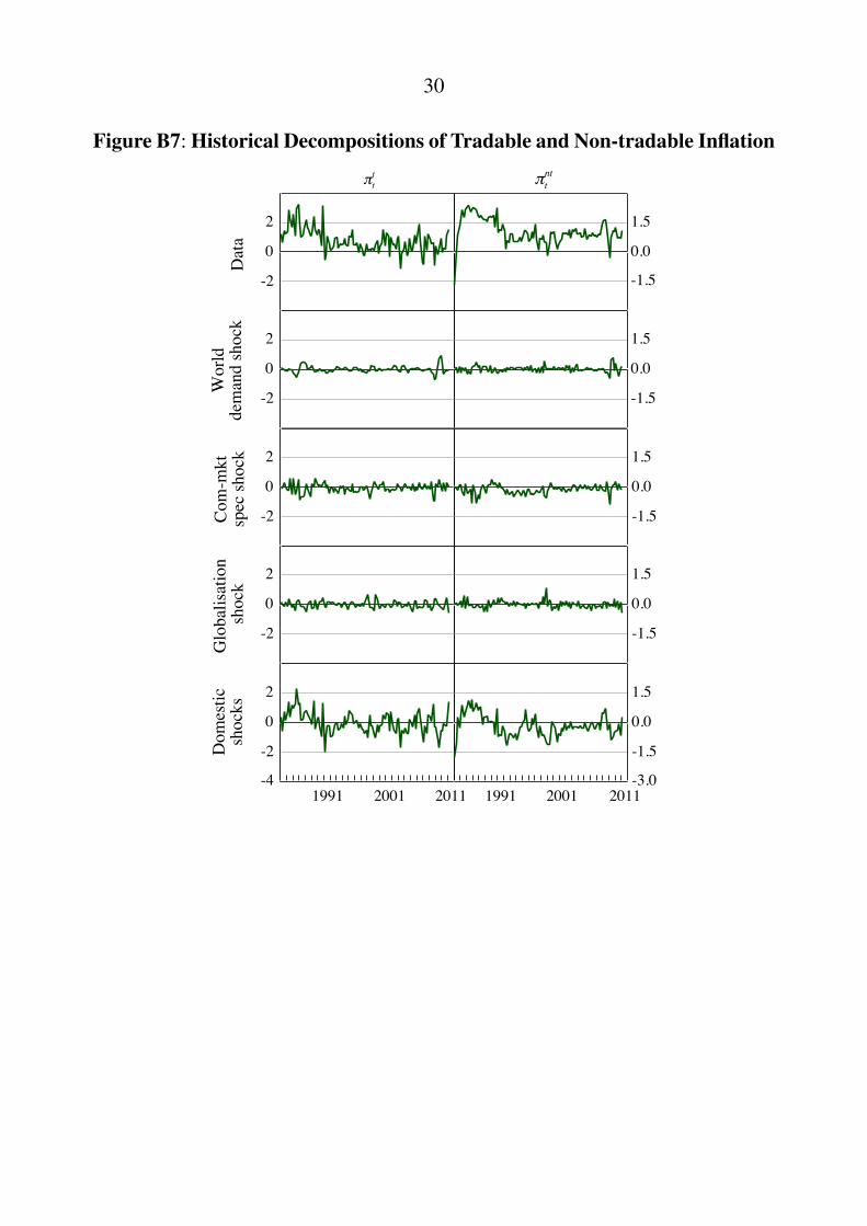
The consumer price index captures the prices of both tradable and non-tradablegoods. Terms of trade shocks will have a direct impact on CPI inflation via theprice of tradable goods but there can be indirect (second round) effects as well.To evaluate the relative importance of direct and indirect effects on inflation, weextend the domestic block of the benchmark VAR to include both non-tradableand tradable inflation in place of trimmed-mean inflation.
The impulse responses of tradable and non-tradable inflation to the three globalshocks are shown in Figure 8. The impulse responses of the remaining variablesin the extended VAR are similar to those presented for the benchmark VAR inFigure 3 and are not shown.
The world demand shock has very little impact upon tradable or non-tradableinflation, consistent with the results for trimmed-mean inflation shown in Figure 3.For the commodity-market specific shock, the negative response of consumerprice inflation appears to be mainly driven by the response of the tradablecomponent, which is slightly offset by the positive response from the non-tradables component. Inflation is initially lower after a globalisation shock.Figure 8 indicates that this is likely to be due to the decline in tradable inflation.However, tradable inflation rises in subsequent periods, perhaps due to thedepreciation of the real exchange rate. The effect of this increase on trimmed-mean inflation is, however, offset by a modest decline in non-tradable inflation.
The variance decompositions for non-tradable and tradable inflation are shown inthe last two columns of Table 3. We do not show the variance decomposition

19
for the world block as this is identical to results presented in Table 2. Notsurprisingly, domestic shocks explain a larger share of non-tradable inflation thantradable inflation. This provides further evidence that the floating exchange ratehas provided an effective buffer to external shocks.
Figure 8: Responses of Tradable and Non-tradable Inflationto Terms of Trade Shocks
Quarters after shock
Non-tradable inflation
■ Percentile bands — Median — Median target
Tradable inflation
Wor
ldde
man
d sh
ock
Com
-mkt
spec
shoc
kG
loba
lisat
ion
shoc
k
-0.2
0.0
0.2
-0.2
0.0
0.2
-0.2
0.0
0.2
-0.2
0.0
0.2
0 5 10 15 20
-0.2
-0.4
0.0
0.2
5 10 15 20
-0.2
-0.4
0.0
0.2
Notes: Figures show the median and median target responses to the different types of terms oftrade shocks, together with the 16th and 84th percentile bands.

20
Table 3: Variance Decomposition: Tradable and Non-tradable InflationPer cent
∆q ∆yd rdπ
ntπ
t
World demand shockMedian target 22 30 13 6 9One std dev interval (18,43) (8,20) (3,20) (4,13) (5,14)
Commodity-market specific shockMedian target 44 8 11 13 18One std dev interval (15,41) (4,13) (2,13) (4,14) (6,17)
Globalisation shockMedian target 3 3 4 8 13One std dev interval (3,11) (4,11) (2,11) (3,12) (4,12)
Shocks to domestic blockMedian target 31 60 72 73 60One std dev interval (27,41) (62,78) (63,85) (67,83) (62,78)
Notes: Results for the world block are unchanged from Table 2 and are not repeated here; πnt is non-tradable
inflation and πt is tradable inflation
4. Conclusion
This paper has provided empirical evidence on the effects of terms of trade shockson inflation, output, interest rates and the real exchange rate in the Australianeconomy. Three shocks to the terms of trade were identified using sign restrictionsin a VAR: a world demand shock that increases export prices, import prices andworld output; a commodity-market specific shock that pushes up export prices,without a corresponding pick-up in world output; and a globalisation shock thatincreases export prices and world output, but reduces import prices.
The main conclusion of this paper is that increases in the terms of trade tend to beexpansionary but are not always inflationary, with the exchange rate providingan effective buffer to external shocks that move the terms of trade. Inflationand output are found to rise following a world demand shock, but this effectis relatively short-lived due to higher interest rates and the appreciation of thereal exchange rate. A commodity-market specific shock, meanwhile, is found toincrease import prices, which results in higher trimmed-mean inflation on impact.The appreciation of the real exchange rate, however, offsets the impact on inflation,which is lower in subsequent periods. Finally, the globalisation shock results in

21
lower domestic inflation on impact but also a depreciation of the real exchangerate, mitigating the deflationary effect in the quarter following the shock.
The terms of trade shocks were found to explain around two-thirds of the variationin the real exchange rate over the sample, but less than one-fifth of variation in theother domestic variables, providing evidence that the floating exchange rate is animportant buffer to these shocks. The globalisation shock was found to be of morelimited empirical importance in explaining movements in the modelled variablesthan the world demand shock or the commodity-market specific shock.
22
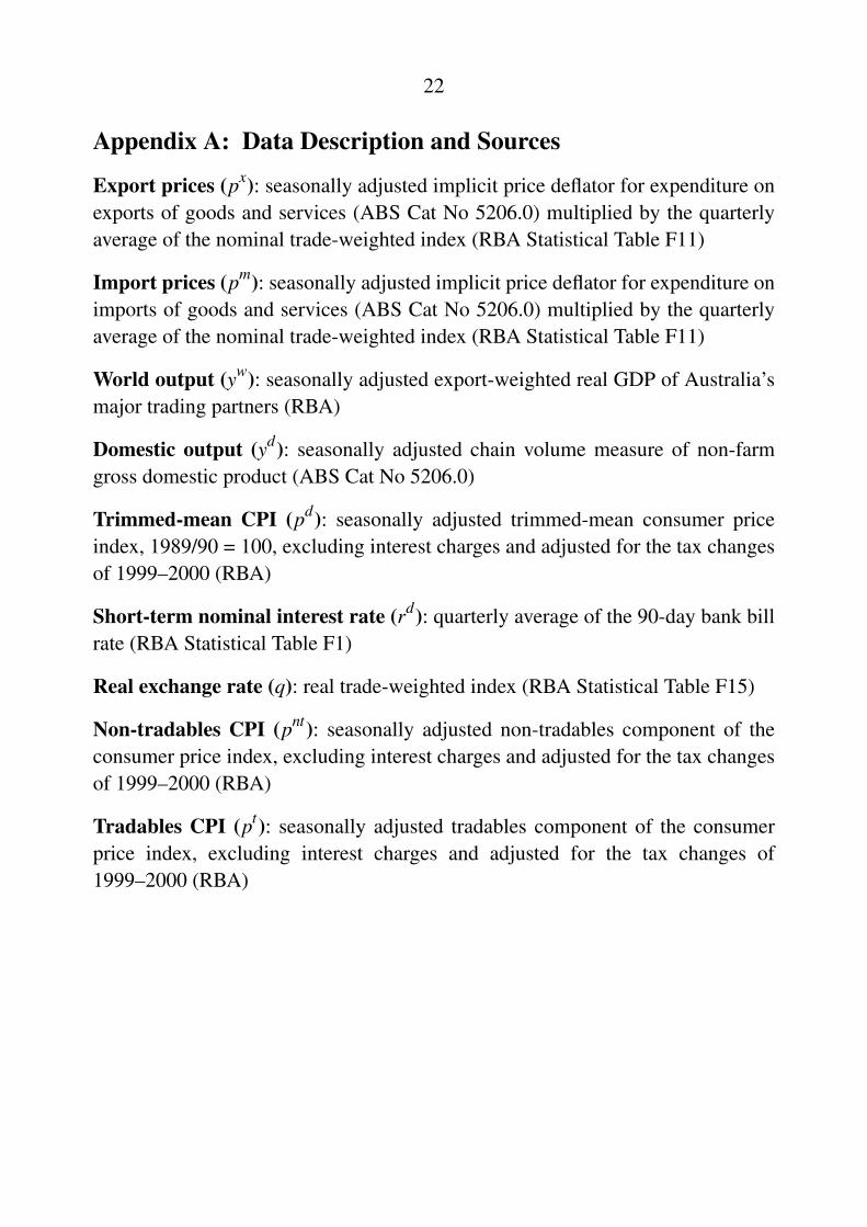
Appendix A: Data Description and Sources
Export prices (px): seasonally adjusted implicit price deflator for expenditure onexports of goods and services (ABS Cat No 5206.0) multiplied by the quarterlyaverage of the nominal trade-weighted index (RBA Statistical Table F11)
Import prices (pm): seasonally adjusted implicit price deflator for expenditure onimports of goods and services (ABS Cat No 5206.0) multiplied by the quarterlyaverage of the nominal trade-weighted index (RBA Statistical Table F11)
World output (yw): seasonally adjusted export-weighted real GDP of Australia’smajor trading partners (RBA)
Domestic output (yd): seasonally adjusted chain volume measure of non-farmgross domestic product (ABS Cat No 5206.0)
Trimmed-mean CPI (pd): seasonally adjusted trimmed-mean consumer priceindex, 1989/90 = 100, excluding interest charges and adjusted for the tax changesof 1999–2000 (RBA)
Short-term nominal interest rate (rd): quarterly average of the 90-day bank billrate (RBA Statistical Table F1)
Real exchange rate (q): real trade-weighted index (RBA Statistical Table F15)
Non-tradables CPI (pnt): seasonally adjusted non-tradables component of theconsumer price index, excluding interest charges and adjusted for the tax changesof 1999–2000 (RBA)
Tradables CPI (pt): seasonally adjusted tradables component of the consumerprice index, excluding interest charges and adjusted for the tax changes of1999–2000 (RBA)

23
Appendix B: Robustness Checks
Figure B1: Responses of World Variables to Terms of Trade ShocksInflation-targeting sample
2
4
6
■ Percentile bands — Median — Median target
2
4
6
5 10 15 20-2
0
2
4
0
1
0
1
-1012
Worlddemand shock
Quarters after shock5 10 15 20
Com-mktspec shock
Globalisation shock
Expo
rt pr
ices
Impo
rt pr
ices
Wor
ld o
utpu
tTe
rms o
f tra
de
210-1
0 5 10 15 20
4
2
0
-2
Notes: Figures show the median and median target accumulated impulse responses to thedifferent types of terms of trade shocks, together with the 16th and 84th percentile bands.The impulse responses for the terms of trade are constructed from the impulse responsesfor export prices and import prices.

24
Figure B2: Responses of Domestic Variables to Terms of Trade ShocksInflation-targeting sample
■ Percentile bands — Median — Median target
Worlddemand shock
Quarters after shock5 10 15 20
Com-mktspec shock
Globalisation shock
Real
exch
ange
rate
Dom
estic
out
put
Infla
tion
rate
Inte
rest
rate
2
0
-2
2
0
-2
0.5
0.0
1.0
0.5
0.0
1.0
0.0
-0.1
0.0
-0.1
0 5 10 15 20
0.5
0.0
-0.5
-1.05 10 15 20
0.5
-0.5
0.0
-1.0
Notes: Figures show the median and median target impulse responses to the different types ofterms of trade shocks, together with the 16th and 84th percentile bands. The accumulatedimpulse responses are shown for output and the real exchange rate.

25
Figure B3: Historical Decompositions of Export and Import Price InflationInflation-targeting sample
-10
0
10
2010
-6
0
6D
ata
-10
0
10
-6
0
6
-10
0
10
-6
0
6
-20
-10
0
10
-12
-6
0
6
Wor
ldde
man
d sh
ock
Com
-mkt
spec
shoc
kG
loba
lisat
ion
shoc
k
20041998201020041998
tx
tm

26
Figure B4: Historical Decompositions of World Output andthe Terms of Trade
Inflation-targeting sample
-1.5
0.0
1.5
2010
-6
0
6
Dat
a
-1.5
0.0
1.5
-6
0
6
-1.5
0.0
1.5
-6
0
6
-3.0
-1.5
0.0
1.5
-12
-6
0
6
Wor
ldde
man
d sh
ock
Com
-mkt
spec
shoc
kG
loba
lisat
ion
shoc
k
20041998201020041998
Change interms of tradeyt
w

27
Figure B5: Historical Decompositions of The Real Exchange Rateand Domestic Output
Inflation-targeting sample
-10
0
10
-1.5
0.0
1.5
Dat
a
-10
0
10
-1.5
0.0
1.5
-10
0
10
-1.5
0.0
1.5
Wor
ldde
man
d sh
ock
Com
-mkt
spec
shoc
kG
loba
lisat
ion
shoc
k
-10
0
10
-1.5
0.0
1.5
2010-20
-10
0
10
-3.0
-1.5
0.0
1.5
20041998201020041998
Dom
estic
shoc
ksqt yt
d

28
Figure B6: Historical Decompositions of Inflation andthe Nominal Interest RateInflation-targeting sample
0
1
0
5
Dat
a
0
1
0
5
0
1
0
5
Wor
ldde
man
d sh
ock
Com
-mkt
spec
shoc
kG
loba
lisat
ion
shoc
k
0
1
0
5
2010-1
0
1
-5
0
5
20041998201020041998
Dom
estic
shoc
kstd rt
d

29
Table B1: Variance DecompositionInflation-targeting sample, per cent
πx
πm
∆yw∆q ∆yd
πd rd
World demand shockMedian target 24 21 55 19 15 10 39One std dev interval (21,45) (12,38) (30,69) (14,37) (12,30) (6,25) (15,52)
Commodity-market specific shockMedian target 69 61 22 49 16 5 5One std dev interval (42,68) (40,69) (15,42) (18,47) (5,18) (5,21) (4,28)
Globalisation shockMedian target 7 18 24 8 11 16 4One std dev interval (6,20) (12,29) (7,37) (4,15) (4,17) (5,20) (2,17)
Shocks to domestic blockMedian target 24 58 69 53One std dev interval (21,42) (45,68) (45,71) (25,59)
30
Figure B7: Historical Decompositions of Tradable and Non-tradable Inflation
-2
0
2
-1.5
0.0
1.5D
ata
-2
0
2
-1.5
0.0
1.5
-2
0
2
-1.5
0.0
1.5
Wor
ldde
man
d sh
ock
Com
-mkt
spec
shoc
kG
loba
lisat
ion
shoc
k
-2
0
2
-1.5
0.0
1.5
2011-4
-2
0
2
-3.0
-1.5
0.0
1.5
20011991201120011991
Dom
estic
shoc
ks
tnt
tt

31
References
Battellino R (2010), ‘Mining Booms and the Australian Economy’, Address toThe Sydney Institute, Sydney, 23 February.
Berkelmans L (2005), ‘Credit and Monetary Policy: An Australian SVAR’, RBAResearch Discussion Paper No 2005-06.
Brischetto A and G Voss (1999), ‘A Structural Vector Autoregression Model ofMonetary Policy in Australia’, RBA Research Discussion Paper No 1999-11.
Canova F and G De Nicolo (2002), ‘Monetary Disturbances Matter for BusinessFluctuations in the G-7’, Journal of Monetary Economics, 49(6), pp 1131–1159.
Connolly E and D Orsmond (2011), ‘The Mining Industry: From Bust to Boom’,in H Gerard and J Kearns (eds), The Australian Economy in the 2000s, Proceedingsof a Conference, Reserve Bank of Australia, Sydney, pp 111–156.
Dungey M and A Pagan (2000), ‘A Structural VAR Model of the AustralianEconomy’, Economic Record, 76(235), pp 321–342.
Dungey M and A Pagan (2009), ‘Extending a SVAR Model of the AustralianEconomy’, Economic Record, 85(268), pp 1–20.
Faust J (1998), ‘The Robustness of Identified VAR Conclusions about Money’,Carnegie-Rochester Conference Series on Public Policy, 49, pp 207–244.
Fry R and A Pagan (forthcoming), ‘Sign Restrictions in Structural VectorAutoregressions: A Critical Review’, Journal of Economic Literature.
Gillitzer C and J Kearns (2005), ‘Long-Term Patterns in Australia’s Terms ofTrade’, RBA Research Discussion Paper No 2005-01.
Gruen D and G Shuetrim (1994), ‘Internationalisation and the Macroeconomy’,in P Lowe and J Dwyer (eds), International Integration of the Australian Economy,Proceedings of a Conference, Reserve Bank of Australia, Sydney, pp 309–363.
IBRD (International Bank for Reconstruction and Development)/WorldBank (2009), Global Economic Prospects 2009: Commodities at the Crossroads,The World Bank, Washington DC.

32
Kilian L (2009), ‘Not All Oil Price Shocks Are Alike: Disentangling Demandand Supply Shocks in the Crude Oil Market’, American Economic Review, 99(3),pp 1053–1069.
Lawson J and D Rees (2008), ‘A Sectoral Model of the Australian Economy’,RBA Research Discussion Paper No 2008-01.
Liu P (2010), ‘The Effects of International Shocks on Australia’s Business Cycle’,Economic Record, 86(275), pp 486–503.
Otto G (2003), ‘Terms of Trade Shocks and the Balance of Trade: There is AHarberger-Laursen-Metzler Effect’, Journal of International Money and Finance,22(2), pp 155–184.
Peersman G (2005), ‘What Caused the Early Millennium Slowdown? EvidenceBased on Vector Autoregressions’, Journal of Applied Econometrics, 20(2),pp 185–207.
Peersman G and I Van Robays (2009), ‘Oil and the Euro Area Economy’,Economic Policy, 24(60), pp 603–651.
Roberts I and A Rush (2010), ‘Sources of Chinese Demand for ResourceCommodities’, RBA Research Discussion Paper No 2010-08.
Rubio-Ramırez JF, DF Waggoner and T Zha (2010), ‘Structural VectorAutoregressions: Theory of Identification and Algorithms for Inference’, TheReview of Economic Studies, 77(2), pp 665–696.
Uhlig H (2005), ‘What Are the Effects of Monetary Policy on Output? Resultsfrom an Agnostic Identification Procedure’, Journal of Monetary Economics,52(2), pp 381–419.