Reserve Bank of Australia

Reserve Bank of AustraliaEconomic Research Department

2009

-06

RESEARCHDISCUSSIONPAPER

Infl ation Volatility and Forecast Accuracy

Jamie Hall and Jarkko Jääskelä

RDP 2009-06

INFLATION VOLATILITY AND FORECAST ACCURACY

Jamie Hall and Jarkko Jaaskela

Research Discussion Paper2009-06

October 2009

Economic Research DepartmentReserve Bank of Australia

We would like to thank Claire Celerier, Tim Hampton, Jeremy Harrison,Johannes Hoffmann, Jesper Johansson, Christopher Kent, Ken Kuttner,Therese Lafleche, Philip Lowe, Kristoffer Nimark, Adrian Pagan, Louise Rickey,Anthony Rossiter and Fabio Rumler for comments and help with the data. Theviews expressed in this paper are those of the authors and do not necessarily reflectthose of the Reserve Bank of Australia. Any errors are our own.

Authors: hallcj or jaaskelaj at domain rba.gov.au

Economic Publications: ecpubs@rba.gov.au

Abstract

This paper examines the statistical properties of inflation in a sample ofinflation-targeting and non-inflation-targeting countries. First, it analyses the time-varying volatility of a measure of the persistent component of inflation. Basedon this measure, inflation-targeting countries (Australia, Canada, New Zealand,Sweden and the United Kingdom) have experienced a relatively more pronouncedfall in the volatility of inflation than non-inflation-targeting countries (Austria,France, Germany, Japan and the United States). But it is hard to say whetherinflation is more volatile in inflation-targeting or non-inflation-targeting countries.Second, it analyses whether inflation became easier to forecast after theintroduction of inflation targeting. It finds that inflation became easier to forecastin both inflation-targeting and non-inflation-targeting countries; the improvementwas greater for the former group but forecast errors remain smaller for the lattergroup.

JEL Classification Numbers: C53, E37Keywords: inflation, time series econometrics

i

Table of Contents

1. Introduction 1

2. Methodology and Data 4

2.1 A Modification of the Stock and Watson Model 5

2.2 Data 6

3. Properties of Inflation 7

3.1 Level of Permanent Components 7

3.2 Time-varying Inflation Volatility 10

4. Forecastability of Inflation 14

5. Conclusion 19

Appendix A: Data Description and Sources 20

Appendix B: Simple Measures of Inflation Behaviour 22

Appendix C: Parameter Estimates 24

Appendix D: Inflation and its Permanent Component 27

Appendix E: Cross-country Estimates of σε 28

Appendix F: GDP Growth Statistics 29

References 30

ii

INFLATION VOLATILITY AND FORECAST ACCURACY

Jamie Hall and Jarkko Jaaskela

1. Introduction

Over the twenty years to 2008, the level and volatility of inflation has declinedacross the world (Table 1). Average CPI inflation across the major countries fellfrom 6.0 per cent over 1977–1992 to 2.0 per cent over 1993–2008, while theunconditional standard deviation fell from 3.7 per cent to 1.6 per cent over thesame period. While these trends are common to all countries, the extent of changehas varied across countries consistent with the tendency for convergence of boththe level and volatility of inflation.1

There is a literature examining the role of monetary regimes in explaining thesechanges, with one particular focus on differences between inflation-targeting(IT) and non-IT regimes (see, for example, Bernanke et al 2001). Others, suchas Geraats (2002), Chortareas, Stasavage and Sterne (2001) and Demertzis andHughes Hallett (2007), study how the precise nature of the policy framework,such as the degree of central bank transparency, is related to the volatility andlevel of inflation. Many of these studies rely on simple measures of inflationbehaviour, such as unconditional means and variances, and are usually based onheadline measures of inflation. However, such measures can be overly influencedby very temporary movements in inflation. This means that the sample period forthe analysis can have an important influence on the results. More importantly,these temporary effects may have little if anything to do with differences in policyframeworks and much more to do with different structural features of the economy,such as its size or openness to trade. One alternative is to focus on underlying orcore measures of inflation. However, there is no widespread agreement on the bestway to do this, and comparable measures across a wide range of countries are not

1 The decline in inflation volatility has not come about because central banks were willing totolerate higher output volatility. In fact, at least over the period up to 2008, output volatilityhas tended to decline (see Table F1; Stock and Watson 2005 and Kent, Smith and Holloway2005). It may be that economies have faced a more benign inflation-output volatility trade-offover this period and/or that policy has played some role – see Cecchetti, Flores-Lagunes andKrause (2006), for example.

2

Table 1: Level and Volatility of Inflation1977–2008 1977–1992 1993–2008

Inflation(a)

Australia 5.00 7.28 2.66Austria 2.89 3.74 2.02Canada 4.09 6.18 1.93France 4.18 6.59 1.70Germany 2.50 3.18 1.80Japan 1.57 2.95 0.14NZ 5.79 9.20 2.26Sweden 4.70 7.69 1.61UK 5.23 7.59 2.79US 4.19 5.64 2.70Average 4.01 6.00 1.96

Inflation volatility(b)

Australia 3.46 3.33 1.44Austria 2.04 2.16 1.48Canada 3.53 3.40 2.08France 3.95 4.20 1.20Germany 2.01 2.23 1.47Japan 2.67 2.85 1.48NZ 5.41 5.59 1.67Sweden 4.63 4.35 2.32UK 4.47 5.12 1.39US 3.01 3.47 1.29Average 3.52 3.67 1.58

Notes: (a) Inflation is measured as the average quarterly change in seasonally adjusted headline CPI expressed onan annualised basis.(b) Volatility is measured by the standard deviation of annualised quarterly inflation.

readily available. Another alternative is to use a statistical model to try to separateheadline inflation into persistent and temporary components.

This paper adopts this latter approach, examining the inflation process in five ITcountries (Australia, Canada, New Zealand, Sweden and the United Kingdom)and five non-IT countries (Austria, France, Germany, Japan and the United States)using a statistical model introduced by Stock and Watson (2007). The Stock andWatson approach decomposes inflation into permanent and transitory components,the variabilities of which are allowed to change over time. Using measures based

3

on this unobserved components stochastic volatility (UC-SV) model, we find littlesupport for sharp distinctions between countries in terms of the level and volatilityof the permanent component of inflation.2

A related approach is to examine the forecastability of inflation.3 An effective andcredible monetary policy regime, other things equal, will help to keep inflationanchored closely around a low and constant mean. By itself, this implies thatinflation should be easier to forecast – that is, forecast errors will tend to be small.

To examine the forecastability of inflation, we used a modified version of theStock and Watson model (M-UC-SV). Following a suggestion of Pagan (2008),we model the time-varying volatilities as autoregressive processes of order one(AR(1)), so that they have finite second moments. And instead of assuming thatthe permanent level of inflation follows a random walk, we use a mean-revertingAR(1), with a freely estimated degree of persistence. These assumptions implythat inflation is a stationary process that can be decomposed into temporaryand persistent (but not permanent) components, consistent with the notion thatmonetary policy can influence inflation and provide a nominal anchor.

In brief, we find that inflation forecastability improved over time across our sampleof selected IT and non-IT countries, both in absolute terms and relative to naıveforecasts. Across countries, the out-of-sample forecast error of the M-UC-SVmodel tends to be somewhat smaller than that of the original UC-SV model.Furthermore, it seems that the improvement in inflation forecastability was morepronounced in IT countries than in non-IT countries.

2 Related work has documented the quantitative effects of inflation targeting. Kuttnerand Posen (2001) document that inflation targeting reduces the persistence of inflation.Benati (2008) concludes that inflation is highly persistent in policy regimes that lack awell-defined nominal anchor. Pivetta and Reis (2007) find that inflation persistence has beenhigh and approximately unchanged in the United States since 1965. Cogley, Primiceri andSargent (2008) argue that this finding can be viewed simply as a manifestation of shifts inaverage (or the target for) inflation. They conclude that inflation persistence has decreased sincethe 1980s.

3 Earlier literature has looked at survey-based inflation expectations. Levin, Natalucci andPiger (2004) find that inflation targeting is effective in anchoring inflation expectations.Johnson (2002) finds that the level of expected inflation in targeting countries falls after theannouncement of targets. However, neither the variability of surveyed inflation expectationsnor the average absolute survey-based forecast error fall after the announcement of targets.

4

The rest of the paper is organised as follows. Section 2 describes the UC-SV modeland its modified version M-UC-SV together with a description of the data used inthe analysis. Section 3 presents the within-sample results on the inflation processbased on the UC-SV model. Section 4 presents results on the forecastability ofinflation where the focus is on the M-UC-SV model. Section 5 concludes.

2. Methodology and Data

Our benchmark model follows Stock and Watson (2007), who characterise theinflation process with an unobserved component model with stochastic volatility(UC-SV). In this model, inflation (πt) is expressed as the sum of a permanentstochastic component (τt) and a transitory innovation component (ηt) as perEquation (1). The permanent component of inflation evolves as a random walkwithout drift as in Equation (2).4 The variance of the shocks (εt) to this componentcan change over time, as can the variance of the transitory innovations.

πt = τt +ηt (1)τt = τt−1 + εt (2)

εt ∼ N(0,σε,t) ηt ∼ N(0,ση ,t)

log(σ2ε,t) = log(σ2

ε,t−1)+νε,t (3)

log(σ2η ,t) = log(σ2

η ,t−1)+νη ,t (4)

νε,t ∼ N(0,γε) νη ,t ∼ N(0,γη)

The relative importance of τ and η is determined by their variances (σ2ε and σ

2η),

which evolve as independent random walks (without drift). The only parametersof the model are γε and γη , which are the standard deviations of νε and νη . Theycontrol the speed at which the size of the permanent and transitory shocks can

4 See also Cogley and Sargent (2001, 2005), Ireland (2007), and Cogley and Sbordone (2008) forpapers that model trend inflation in this way.

5

change. If all the νi,t shocks were zero after date t0, then the variances σ2ε and σ

2η

would stay fixed at their date t0 values, and the model would simply become arandom walk observed with noise, as in Equations (1) and (2).

Using Equations (1) to (4), we can estimate the evolution of τt , σ2ε,t and σ

2η ,t ,

conditional on inflation data (πt).5 It is possible to set the values of γε and γη by

calibration – Stock and Watson (2007, 2008) use this approach – but we chose toestimate them, and thereby allow for cross-country variation in our analysis.

2.1 A Modification of the Stock and Watson Model

This section describes a modified version of the UC-SV model (M-UC-SV), whichin principle should be preferred when looking at questions related to forecasts.While the model of Stock and Watson (2007, 2008) provides a useful way toassess the within-sample properties of the inflation process, it is less satisfactoryfor questions related to forecastability. In particular, their model implies thatinflation has a unit root and the variances of the permanent and the transitorycomponents are unbounded, so the model becomes explosive over longer horizons(Pagan 2008; Bos, Koopman and Ooms 2007).6

The M-UC-SV model relaxes the assumption that the permanent component ofinflation is a random walk, and assumes instead that there are persistent shocksaround a fixed mean (µ):

πt = µ + τt +ηt (5)τt = φτt−1 + εt (6)

where φ is constrained to be less than one in absolute value. This constraint rulesout an explosive root in inflation.

We also allow univariate stochastic volatility processes to evolve asauto-regressive processes:

log(σ2η ,t) = ρ log(σ2

η ,t−1)+νη ,t (7)

5 To do this we apply the Gibbs sampler.6 If the model is used to simulate 50 years’ worth of data, starting from initial values calibrated

for the United States, at least one hyperinflation is very likely.

6

log(σ2ε,t) = ρ log(σ2

ε,t−1)+νε,t (8)

This assumption forces the variances of the persistent (εt) and temporary (ηt)components of inflation to be bounded; we estimate µ and φ using the Gibbssampler, but calibrate ρ to 0.98.7 In this model, if the νi,t shocks were set to zeroafter period t0, then the logs of σ

2ε and σ

2η would converge to zero, meaning that

their levels would approach one, so that the ε and η shocks in Equations (7) and(8) would become standard normals.

Our focus will be on the time-varying volatilities σ2η and σ

2ε . For completeness,

Tables C1, C2 and C3 in Appendix C provide estimates of µ , φ , γε and γη for thecountries in our sample.

2.2 Data

We use CPI series that are corrected (where possible) for changes to indirecttaxation (and the direct effects associated with changes in interest rates).8 In somecases it is not possible to correct inflation for the effects of movements in indirecttaxes. We provide more details in Appendix A. For the United Kingdom we usedthe retail price index excluding mortgage interest (RPIX).

Where possible, we use data commencing in 1960. As described in Appendix A,we used seasonally adjusted quarterly data. Some countries publish seasonallyadjusted CPI series; for the remainder, we used X-12-ARIMA to remove theseasonal component.9

7 We tried including a freely-estimated mean and AR(1) coefficient in Equations (7) and (8), butthe Gibbs sampler became numerically unstable. Models with calibrated values of ρ between0.9 and 0.99 are hard to distinguish; lower calibrated values produce slightly worse forecastingperformance, and are not as stable numerically.

8 We also performed the analysis using central bank ‘preferred’ measures of inflation (whereapplicable), such as the personal consumption expenditure deflator for the United States. Ingeneral, the results are broadly similar to those presented below.

9 Monthly data were seasonally adjusted if needed and then converted to quarterly data by takingaverages of the monthly observations.

7

3. Properties of Inflation

3.1 Level of Permanent Components

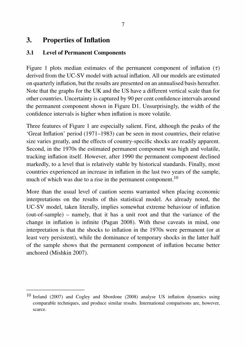
Figure 1 plots median estimates of the permanent component of inflation (τ)derived from the UC-SV model with actual inflation. All our models are estimatedon quarterly inflation, but the results are presented on an annualised basis hereafter.Note that the graphs for the UK and the US have a different vertical scale than forother countries. Uncertainty is captured by 90 per cent confidence intervals aroundthe permanent component shown in Figure D1. Unsurprisingly, the width of theconfidence intervals is higher when inflation is more volatile.

Three features of Figure 1 are especially salient. First, although the peaks of the‘Great Inflation’ period (1971–1983) can be seen in most countries, their relativesize varies greatly, and the effects of country-specific shocks are readily apparent.Second, in the 1970s the estimated permanent component was high and volatile,tracking inflation itself. However, after 1990 the permanent component declinedmarkedly, to a level that is relatively stable by historical standards. Finally, mostcountries experienced an increase in inflation in the last two years of the sample,much of which was due to a rise in the permanent component.10

More than the usual level of caution seems warranted when placing economicinterpretations on the results of this statistical model. As already noted, theUC-SV model, taken literally, implies somewhat extreme behaviour of inflation(out-of-sample) – namely, that it has a unit root and that the variance of thechange in inflation is infinite (Pagan 2008). With these caveats in mind, oneinterpretation is that the shocks to inflation in the 1970s were permanent (or atleast very persistent), while the dominance of temporary shocks in the latter halfof the sample shows that the permanent component of inflation became betteranchored (Mishkin 2007).

10 Ireland (2007) and Cogley and Sbordone (2008) analyse US inflation dynamics usingcomparable techniques, and produce similar results. International comparisons are, however,scarce.

8

Figure 1: Inflation and its Permanent Component

0

10

20Australia

0

10

20

0

10

20

0

10

20

Austria

FranceCanada

0

10

20

0

10

20

0

10

20

0

10

20

0

10

20

0

10

20

Germany Japan

NZ Sweden

-100

102030

-5051015

USUK

19931978 2008

% %

%

%

%

%

%

%

%%

1963 19931978 2008

– Inflation – Permanent component

Bernanke (2007) interprets Stock and Watson’s results as evidence that inflationexpectations in the United States were better anchored after 1990 than from 1970to 1980, due to improvements in monetary policy. The results shown in Figure 1are consistent with the same conclusion for all the countries in our sample;although there may be other plausible explanations (including the absence of largeinflation shocks).

Table 2 reports simple summary statistics for the permanent component ofinflation, τ . The first row for each country shows the sample average, τ . The

9

Table 2: Level and Volatility of the Permanent Component of Inflation1960–2008 1977–1992 1993–2008 Change

(I) (II) (III) (III)-(II)Australia τ 5.88 7.68 2.66 –5.02

στ 3.77 2.32 0.89στ/σπ 0.85 0.75 0.62

Austria τ 3.50 3.79 2.11 –1.68στ 1.84 1.42 0.91

στ/σπ 0.66 0.64 0.60Canada τ 4.14 6.38 1.98 –4.40

στ 3.02 2.86 0.88στ/σπ 0.86 0.87 0.44

France τ 4.73 6.91 1.71 –5.20στ 3.75 3.94 0.72

στ/σπ 0.95 0.96 0.61Germany τ 2.88 3.07 1.89 –1.18

στ 1.80 1.93 1.07στ/σπ 0.82 0.84 0.72

Japan τ 3.20 2.97 0.21 –2.76στ 3.18 2.08 0.89

στ/σπ 0.63 0.72 0.56NZ τ 6.69 9.74 2.20 –7.54

στ 5.39 5.22 1.24στ/σπ 0.98 0.97 0.75

Sweden τ 4.84 7.74 1.61 –6.13στ 3.33 2.40 1.50

στ/σπ 0.74 0.58 0.65UK τ 5.60 7.55 2.46 –5.09

στ 5.17 4.30 0.74στ/σπ 0.94 0.88 0.73

US τ 4.14 5.79 2.73 –3.06στ 2.83 3.30 0.78

στ/σπ 0.95 0.94 0.62

10

second row gives the sample standard deviation of τ . The third row shows theratio of that standard deviation to the standard deviation of inflation. The resultsshow that the average of the permanent component after 1992 fell in all countries.It also appears that in the latter part of the sample, the permanent component ofinflation converged somewhat across countries. Furthermore, the sample standarddeviation of τ clearly fell in all countries between the first and second parts ofthe sample. Over time, the volatility of the permanent component tended to fallsomewhat relative to the volatility of overall inflation for most, though not all,countries.

3.2 Time-varying Inflation Volatility

We turn now to the estimated time series of the volatilities of the permanent andtransitory shocks to inflation, that is, σ

2ε,t and σ

2η ,t . (Note that these volatilities

should not be confused with γ2ε and γ

2η , which govern the magnitude of the

time-variation in σ2ε,t and σ

2η ,t .)

The time profiles of σε,t and ση ,t are shown in Figure 2. Figure 3 showsthe ratio of the standard deviation of the permanent shocks to the sum of thestandard deviations of the temporary and permanent shocks, that is, σε,t

ση ,t+σε,t(with

90 per cent confidence intervals).

Across most countries in the sample, the high-inflation episodes of the 1970swere characterised by a relatively high level of variance of the permanent shocks,which had fallen by the mid 1990s. One interpretation is that the decline in thevolatility of the permanent shocks (Figure 2) is evidence of a decrease in inflationuncertainty. Interestingly, the rise in the level of the permanent component ofinflation in the 1970s (Figure 1) was matched by an increase in the volatility ofthe permanent shocks (Figure 2). The most recent estimates of the volatility of thepermanent shocks are still very close to the sample lows in each country.

11

Figure 2: Median Estimates of the Standard Deviations of the Permanent(σε) and Temporary (ση) Components of Inflation

– Estimate of σε – permanent – Estimate of ση – temporary

2008

Austria

France

Japan

Sweden

US

200819930

2

4

2

4

5

10

5

10

2

4

2

4

1978

Australia

Canada

Germany

UK

NZ

0

2

4

2

4

1

2

2

4

2

4

1963 19931978

Focusing on the United States first, Figures 2 and 3 suggest that its monetary policywas less successful in stabilising inflation during the 1970s than at other times; thisis reflected in the relative and absolute rise of σε in the 1970s. A similar patterncan be discerned in other countries, although there are some differences acrosscountries. These differences will in part be due to the inherent uncertainty that isan explicit feature of any econometric estimates such as provided by the UC-SVmodel (but are not captured by more simplistic measures of underlying inflation

12

trends). They are also likely to reflect differences in circumstances and institutionsacross the countries in our sample. Nevertheless, at least over more recent years,the relative importance of the volatility of the permanent shocks has been low inall countries – σε remained below ση – and the estimated level of σε has beengenerally low relative to the uncertainty surrounding the estimate (see Table E1).This means that it is difficult to distinguish between different policy regimes basedon the behaviour of the permanent component of inflation.

Figure 3: Ratio of the Standard Deviation of the Permanent Shocks to theSum of the Standard Deviations of the Temporary and Permanent Shocks

0.0

0.5

1.0

0.0

0.5

1.0

0.0

0.5

1.0

0.0

0.5

1.0

0.0

0.5

1.0

0.0

0.5

1.0

0.0

0.5

1.0

Australia Austria

France

Japan

Canada

Germany

0.0

0.5

1.0

0.0

0.5

1.0

-0.5

0.0

0.5

1.0

-0.5

0.0

0.5

1.0

0.0

0.5

1.0SwedenNZ

UK US

– Estimated ratio – 90% confidence interval

19931978 20081963 19931978 2008

13

In order to shed more light on possible differences between IT andnon-IT countries, we can compare estimates of the distribution of the permanentcomponent of inflation across these two groups over time. Specifically, we lookat four time periods: one before, one around, and two after the introductionof inflation targeting (exactly which dates we look at does not affect the keyconclusions from this exercise).11 At any point in time, we have an estimate ofthe distribution for the standard deviation of the permanent component of inflation(the median of each of these is shown in Figure 2 above). So, it is straight forwardto combine these distributions across countries within the IT and non-IT groups,assigning equal weight to all countries within each group, as shown in Figure 4.

Figure 4: Estimated Density for Standard Deviation of the PermanentComponent (σε)

– IT countries – Non-IT countries

0.00

0.05

0.10

0.15

0.00

0.05

0.10

0.15

0.05

0.10

0.15

0.05

0.10

0.15

0.05

0.10

0.151987:Q1 1993:Q1

2000:Q3 2008:Q2

0.00

0.05

0.10

0.15

0.00

0.05

0.10

0.15

320 1 4321

From this figure we can see some evidence that after 1993 the distribution ofthe standard deviation of the permanent shocks to inflation narrowed, particularly

11 The adoption date of inflation targeting varies from country to country. Kuttner (2004) datesinflation targeting to have begun in: Australia in March 1993; Canada in February 1991;New Zealand in December 1989; Sweden in January 1993; and the UK in October 1992. Allhad adopted the inflation-targeting framework by 1993:Q1. Classifying countries as inflationand non-inflation targeters can seem a bit arbitrary, particularly for countries in Europe in therun-up to monetary union, which entailed explicit targets for inflation.

14

for IT countries. This suggests that inflation targeters became better at managingshocks hitting the economy than in the past (including, perhaps, by contributingless to monetary policy shocks) and are now comparable to non-targeters, whoalso improved on this score. This is consistent with Truman (2003), who finds ITcountries experienced larger declines in inflation volatility, but with differences ininitial conditions for IT and non-IT countries. Of course, caution should be usedin interpreting the results. For example, we are unable to determine the extent towhich these changes were simply due to good luck.

4. Forecastability of Inflation

Low and stable inflation should imply that inflation is relatively easy to forecast.So it makes sense when comparing outcomes in IT and non-IT economies toconsider how easy it is to forecast inflation, particularly over horizons of abouttwo years, by which time monetary policy could be expected to have had timeto control inflation in response to a particular shock. In this section of the paperwe compare the accuracy of out-of-sample forecasts across countries and overtime within countries using different models. As discussed above, using theUC-SV model in this way is potentially problematic, notwithstanding itswithin-sample fit. We pay particular attention to comparing the out-of-sampleforecasting performance of the UC-SV and M-UC-SV models.

In this exercise we estimate each model using data available at a given date t,and computing a h-period-ahead forecast for date t +h, then moving forward oneperiod (to t + 1), and so on. We use a rolling ten-year window to estimate themodels and generate inflation forecasts for eight quarters in the future.12 For eachmodel, this gives us a series of forecast errors for each country. These series arethen pooled together for inflation targeters and non-targeters; in order to comparehow the forecasting performance has changed over time we split the 48-yearsample in half.

Table 3 summarises the results of this out-of-sample forecasting exercise, anddisaggregates these results according to monetary policy regime. For both models,the root mean squared error (RMSE) fell substantially from the first to the second

12 The permanent component of inflation provides a h-period-ahead forecast measure of inflation(πt+h|t = τt|t) for the UC-SV model. In the autoregressive version, the forecast is anexponentially weighted average of the persistent deviation τt and the permanent level µ .

15

half of the sample period, indicating that inflation became much easier to forecast.IT countries experienced a slightly better improvement in RMSE compared tonon-IT countries, but, on average, forecast errors remain slightly smaller in thenon-IT country sample.

Table 3: Root Mean Squared ErrorsPer cent – annualised

1977–1992 1993–2008Inflation targeters UC-SV 4.53 2.19

M-UC-SV 4.61 2.29Non-targeters UC-SV 3.34 1.63

M-UC-SV 3.38 1.55

Figures 5 and 6 plot the actual change in inflation against the forecasted change.Because there are too many data points for a scatterplot to be meaningful, we showthe contours of kernel density estimates instead. Following Theil (1966), the plotsfocus on the forecast of the change in inflation, rather than the forecast of its level,for several reasons: this puts the focus on predicting turning points, which is bothharder and arguably more useful than predicting a continuing trend; it circumventsthe problem of rescaling and demeaning the observations; and it makes it easy tovisualise the naıve forecast (∆πt+8 = 0) that we use as a benchmark. To interpretthese, note that a naıve forecast (which has πt+8|t = πt) would generate pointsalong the horizontal axis, while a perfect forecast would be a 45◦ line through theorigin. The solid line shows the line of best fit through each set of points. Thegradient of this line of best fit is comparable to the forecastability measures ofTheil (1966). It indicates how far the model’s average performance is from that ofa perfect forecasting model, with a value of one corresponding to perfection and avalue of zero indicating failure.

These figures confirm that inflation became easier to forecast from the first halfof the sample to the second; both lines of best fit for each model are closerto the 45◦ line. Overall, it seems that the M-UC-SV model’s forecasts are lessbiased, at the cost of lower precision. This is evidenced by the fact that its lineof best fit (solid line) is steeper than that of the UC-SV (M-UC-SV forecasts aremore accurate on average), while the contours around these solid lines are wider(M-UC-SV forecasts are less precise). In other words, the UC-SV’s forecasts of

16

Figure 5: Forecasting Performance1977–1992

-15

-10

-5

0

5

10

15

-15 -10 -5 0 5 10 15

UC–SV model

∆π – actual

∆π – predicted

-15

-10

-5

0

5

10

15

-10 -5 0 5 10 15 ∆π – actual

∆π –

pre

dict

edM–UC–SV model

Figure 6: Forecasting Performance1993–2008

-15

-10

-5

0

5

10

15

-15 -10 -5 0 5 10 15

UC–SV model

∆π – actual

∆π – predicted

-15

-10

-5

0

5

10

15

-10 -5 0 5 10 15 ∆π – actual

∆π –

pre

dict

ed

M–UC–SV model

∆πt+8 are biased towards zero. The bias for both models is somewhat lower in thelatter period of low and stable inflation.

Table 4 reports the slope of the line of best fit, calculated as for Figures 5 and 6.The results suggest that inflation became easier to forecast across the board.

In order to investigate more carefully the relative performance of the UC-SVmodel and its M-UC-SV version, we provide a country-by-country breakdown ofthe forecast performance in Table 5, based on the RMSE. Table 5 also reportsthe forecast performance of a naıve forecast for inflation eight quarters in thefuture (πt+8|t) based on the most recently observed value (πt). In other words,it always predicts no change in inflation. We also present the RMSEs of a

17

Table 4: The Bias of Inflation Forecasts1977–1992 1993–2008

Inflation targeters UC-SV 0.16 0.29M-UC-SV 0.37 0.46

Non-targeters UC-SV 0.07 0.29M-UC-SV 0.34 0.50

Note: The bias is measured by the slope of the line of best fit for ∆πt+8|t regressed on ∆πt+8.

benchmark provided by the Atkeson and Ohanian (2001) (AO) model, whereby theeight-quarter-ahead inflation rate is forecast as the average rate of inflation over theprevious four quarters.13

We chose the AO model as a benchmark as it is hard to beat.14 Consider twoextremes. If inflation were a random walk, the best forecast would be the currentvalue of inflation (the naıve method), but the AO model would also do reasonablywell. In contrast, if inflation was subject only to purely transitory shocks, thenaıve method would do poorly, while again the AO model should do reasonablywell. The M-UC-SV model should perform relatively well in situations whereinflation experiences persistent (but not permanent) deviations from a relativelystable mean. Also, one advantage of the UC-SV and M-UC-SV models is thatthey can accommodate changes in the volatility of the persistent and transitorycomponents.

Together, the two models outperform the AO benchmark in most countries in bothsample periods. For Australia in the more recent sample period, the AO modelperforms best, and across all models the RMSE for Australia is comparable tothose of Austria, Japan, the United Kingdom and the United States, and lower thanfor Canada, New Zealand and Sweden. Across all countries, the performance ofthe M-UC-SV is comparable to that of the UC-SV model. Excluding the countries

13 Here we follow Stock and Watson’s (2007) interpretation of Atkeson and Ohanian (2001).

14 Stock and Watson (2007, 2008) provide a comprehensive review of the forecasting performanceof many inflation models (a total of 157 distinct models). They report that there is no singlemodel, nor combination of univariate models, that has uniformly better performance than theUC-SV model, at least for quarterly US data. Canova (2007) focuses on CPI inflation in G7countries and finds that the performance of univariate time-varying parameter models is hardlyany different than that of more complicated model specifications.

18

Table 5: Root Mean Squared Errors1977–1992 1993–2008

Australia AO 4.23 1.67Naıve 4.51 2.24

UC-SV 3.77 1.81M-UC-SV 4.05 2.10

Austria AO 2.57 1.70Naıve 3.09 2.08

UC-SV 2.81 1.64M-UC-SV 2.34 1.56

Canada AO 3.44 2.51Naıve 3.63 3.11

UC-SV 3.46 2.45M-UC-SV 4.30 2.48

France AO 3.37 1.37Naıve 3.43 1.76

UC-SV 3.32 1.34M-UC-SV 4.53 1.54

Germany AO 2.64 1.84Naıve 2.75 2.27

UC-SV 2.65 1.82M-UC-SV 2.60 1.61

Japan AO 3.63 1.80Naıve 3.86 2.16

UC-SV 3.56 1.73M-UC-SV 3.17 1.56

NZ AO 6.10 2.14Naıve 6.83 2.42

UC-SV 6.62 2.14M-UC-SV 5.56 2.17

Sweden AO 4.74 2.85Naıve 5.69 2.91

UC-SV 4.59 2.86M-UC-SV 5.09 2.96

UK AO 3.10 1.69Naıve 3.55 1.59

UC-SV 3.35 1.44M-UC-SV 2.72 1.53

US AO 2.06 1.60Naıve 4.21 1.85

UC-SV 4.12 1.57M-UC-SV 3.78 1.47

19

where both models fail to beat the AO benchmark, the M-UC-SV is preferred tothe UC-SV model in a majority of countries.

The ability of these models to outperform the AO benchmark in a range ofcountries is evidence against the conclusions of recent econometric studies(including Stock and Watson 2007). That literature suggests that inflation becameeasier to forecast in the sense that the size of RMSEs had fallen (as in Table 3above) and that more stable inflation makes the AO model a harder benchmark tobeat. By contrast, in our second sample period, the AO model is clearly superiorin only one out of ten countries; the last few years of the sample show a rise inthe persistent component of inflation for most countries, which the UC-SV andM-UC-SV models should capture better than the AO model.

5. Conclusion

This paper compares the statistical properties of inflation in a sample of IT andnon-IT countries using an unobserved components stochastic volatility model(UC-SV) proposed by Stock and Watson (2007). This approach decomposesinflation into permanent and transitory components and allows the variabilityof both components to change over time. We find that IT countries (Australia,Canada, New Zealand, Sweden and the United Kingdom) on average experienceda more pronounced fall in the volatility of the permanent component of inflationthan non-IT countries (Austria, France, Germany, Japan and the United States), tolevels that are now broadly comparable.

We also propose a modification of the original UC-SV model in order to allowfor more plausible implied properties of inflation which are particularly desirablewhen forecasting inflation. We find that inflation became easier to forecast inboth IT and non-IT countries since the early 1990s, but forecast errors remainedsomewhat smaller in the latter group. Across the countries in our sample, forecastsfrom the modified UC-SV model are generally superior to those based on theassumption that the eight-quarter-ahead inflation rate is the average rate ofinflation over the previous four quarters.

20

Appendix A: Data Description and Sources

Australia: Consumer price index excluding interest and tax, 1969–2008(quarterly), available from the Reserve Bank of Australia. Mortgage interestcharges were removed from the published CPI basket in 1998:Q3; we used arecalculated headline series that removed those charges from the earlier part ofthe sample. The introduction of a Goods and Services Tax (GST) in 2000 causedan inflationary spike that is not considered significant for the purposes of monetarypolicy, so we used a series that corrects for this effect. For further details on theseries, see Roberts (2005) and Brischetto and Richards (2006).

Austria: CPI for average wage-earning households (Series I), 1959–2008(monthly), available from Statistik Austria. For our analysis, we seasonallyadjusted the series and then converted it to a quarterly frequency. When Austriajoined the European Union in 1995, changes in food subsidies caused a drop inCPI. However, we have not corrected for this effect.

Canada: Headline CPI, 1960–2008. For our analysis, we seasonally adjusted theseries. Ideally, we would correct for the effects of indirect taxes, but the publishedindex that does this, the CPIXFET series, also excludes food and energy. Forfurther details on the Bank of Canada’s preferred inflation measure, see Laflecheand Armour (2006).

France: CPI, 1960–2008 (monthly), available from Eurostat, and fromDatastream (code FRCP....F). For our analysis, we seasonally adjusted the seriesand then converted it to a quarterly frequency. There have been four relativelyminor changes to Value Added Tax (VAT) in recent history; we did not adjustthe CPI for these. (In January 1977, the VAT rate decreased from 20 per centto 17.6 per cent; in July 1982, it increased to 18.6 per cent; in August 1995, itincreased to 20.6 per cent; and in April 2000, it fell to 19.6 per cent.) The Banquede France focuses on the Harmonised Index of Consumer Prices (HICP), HICPexcluding food and energy and HICP excluding administered prices. However,these series have not been included in our study, because of their short timespan. Statistical measures have also been considered, but rejected for their lackof economic meaning (Bihan and Sedillot 1999).

Germany: CPI for the Federal Republic of Germany, January 1960–2008(monthly), available from Statistisches Bundesamt Deutschland. Prior to 1991, we

21

used West German data. For our analysis, we seasonally adjusted the series andthen converted it to a quarterly frequency. Numerous changes to VAT have beenmade during the period under consideration, but they are likely to have had smallfirst-round effects on inflation (Hoffmann and Hofmann 2004). The exceptionis the VAT change of January 2007, which had significant first-round effects;however, those effects were smoothed over a twelve-month period beginninghalf a year before the tax change, and were entangled with second-round effects(Deutsche Bundesbank 2008).

Japan: All Japan CPI, 1975–2008, monthly, corrected for the VAT change in April1997. For our analysis, we seasonally adjusted the series and then converted it toa quarterly frequency.

New Zealand: GST-corrected CPI (PCPIG), 1975–2008, quarterly, availablefrom the Reserve Bank of New Zealand; supplemented with the headline CPI(Datastream code NZCP....F) prior to 1975. The PCPIG excludes the direct priceeffects of the introduction of GST in 1986 and the increase in 1989. For ouranalysis, we seasonally adjusted the series.

Sweden: CPI, 1960–2008, available from Statistics Sweden. Indirect taxescontributed around 1.5 per cent to the monthly changes in CPI in March 1990and January 1991 and 1993, and subtracted around 1.2 per cent from the monthlychanges in CPI in January 1992. The published CPIX measure removes theseeffects, along with mortgage interest charges. We used the headline measure inour analysis because of its longer available span and seasonally adjusted it.

United Kingdom: Retail prices index excluding mortgage interest payments(RPIX), 1975–2008, monthly; we seasonally adjusted the series and thenconverted it to a quarterly frequency.

United States: CPI, 1960–2008, all urban consumers (CPI-U), seasonallyadjusted, available from the bureau of Labor Statistics; converted to a quarterlyfrequency for our analysis.

22

Appendix B: Simple Measures of Inflation Behaviour

Table B1 shows a collection of simple measures that could be used to evaluatecentral bank performance. The ‘Headline’ columns are based on the year-endedgrowth in the data series that were described in Appendix A. The ‘Core’ columnsuse the following data series: Australia, trimmed mean CPI (15 per cent trim);Canada, CPI excluding food, energy and indirect taxes; Japan, All Cities CPIexcluding fresh food; New Zealand, PCPITA, the CPI measure being targetedin a given quarter; Sweden, CPI excluding mortgage interest payments; UK,RPIX until 2003:Q2, with CPI thereafter; US, personal consumption expendituresdeflator.

Table B1: Inflation BehaviourMean Std dev MAD Outside band

Headline Core Headline Core Headline Core Headline CoreIT countries

Australia 2.54 2.26 0.68 0.42 0.51 0.37 25 16Canada 2.08 1.87 1.29 0.66 0.88 0.53 17 5NZ 2.28 2.21 1.30 0.81 1.06 0.68 26 19Sweden 1.47 1.69 1.35 0.87 1.16 0.78 31 21UK 2.61 2.39 0.80 0.51 0.87 0.53 22 1

Non-IT countriesAustria 1.94 0.85 0.68

France 1.61 0.56 0.42

Germany 1.73 0.93 0.66

Japan 0.11 –0.03 0.85 0.59 0.64 0.45

US 2.60 2.08 0.67 0.59 0.54 0.46

Notes: Following Kuttner (2004), we chose samples that begin as follows: Australia, at 1993:Q1; Canada, at1991:Q1; New Zealand, at 1989:Q4; Sweden, at 1993:Q1; and the UK, at 1992:Q4. The samples for non-IT countries begin in 1993:Q1. All the samples end in 2007:Q1. For a description of the various core (orunderlying) measures see main text above.

The ‘Mean’ and ‘Std dev’ columns show the sample mean and sample standarddeviation of inflation during the period in question. For IT countries, ‘MAD’ isthe mean absolute deviation from the centre of the target band; and ‘Outside

23

band’ is the number of quarters during which the inflation measure was outsidethe target, allowing for changes to the target band where appropriate. Australiatargets a headline inflation rate of 2 to 3 per cent on average over the businesscycle; Canada targets 2 per cent inflation in headline CPI, with a range of1 to 3 per cent; New Zealand initially targeted a range of 3 to 5 per cent,then 0 to 2 per cent from 1992 to 1996, then 0 to 3 per cent from 1997to 2001, then 1 to 3 per cent from 2002 onwards; Sweden targets 2 percent inflation, with a tolerance interval of 1 per cent either side (the target,announced in 1993, became effective in 1995); and the UK initially targeted1 to 4 per cent RPIX inflation (with an objective to be in the lower half ofthat range by the end of the 1992–1997 Parliament), then 2.5 per cent RPIXinflation with a tolerance interval of 1 per cent either side from 1996 to 2003,then 2 per cent CPI inflation from 2004 onwards, with a formal explanationrequired for deviations of more than 1 per cent either side of the target. Fornon-IT countries, the ‘MAD’ column is the mean absolute deviation from thesample mean.

24

Appendix C: Parameter Estimates

Table C1: Parameter EstimatesFull sample

Mean 5% 95% Mean 5% 95% Mean 5% 95%Australia Austria Canada

φ 0.29 0.01 0.97 0.08 0.01 0.26 0.33 0.02 0.94µ 0.79 0.61 0.98 0.56 0.45 0.68 0.54 0.43 0.69γε 0.25 0.16 0.39 0.25 0.16 0.39 0.26 0.16 0.39γη 0.28 0.18 0.39 0.34 0.24 0.39 0.36 0.29 0.39γ?ε 0.25 0.10 0.39 0.13 0.10 0.27 0.19 0.10 0.39

γ?η 0.38 0.37 0.39 0.39 0.37 0.39 0.38 0.36 0.39

France Germany Japanφ 0.32 0.01 0.98 0.17 0.02 0.66 0.90 0.70 0.98µ 0.54 0.34 0.80 0.44 0.36 0.53 0.17 -0.08 0.46γε 0.26 0.16 0.39 0.25 0.16 0.39 0.35 0.24 0.39γη 0.32 0.23 0.39 0.36 0.29 0.39 0.39 0.37 0.39γ?ε 0.23 0.10 0.39 0.19 0.10 0.39 0.15 0.10 0.37

γ?η 0.31 0.10 0.39 0.38 0.35 0.39 0.38 0.36 0.39

NZ Sweden UKφ 0.36 0.01 0.98 0.52 0.01 0.99 0.41 0.01 0.98µ 0.53 0.20 0.77 0.56 0.25 1.01 0.62 0.05 0.83γε 0.28 0.16 0.39 0.30 0.17 0.39 0.27 0.16 0.39γη 0.36 0.28 0.39 0.38 0.33 0.39 0.26 0.12 0.39γ?ε 0.37 0.27 0.39 0.29 0.10 0.39 0.26 0.12 0.39

γ?η 0.29 0.10 0.39 0.39 0.38 0.39 0.34 0.13 0.39

USφ 0.09 0.01 0.26µ 0.62 0.52 0.74γε 0.24 0.16 0.38γη 0.29 0.20 0.39γ?ε 0.24 0.10 0.39

γ?η 0.30 0.11 0.39

Note: ? parameters are from the UC-SV model; other parameters are from the M-UC-SV model

25

Table C2: Parameter Estimates1977:Q3–1992:Q4

Mean 5% 95% Mean 5% 95% Mean 5% 95%Australia Austria Canada

φ 0.22 0.02 0.64 0.17 0.01 0.54 0.22 0.02 0.65µ 1.45 1.10 1.75 0.77 0.58 0.94 1.09 0.85 1.33γε 0.27 0.15 0.39 0.25 0.14 0.39 0.26 0.14 0.39γη 0.19 0.10 0.35 0.22 0.11 0.38 0.20 0.10 0.35γ?ε 0.18 0.10 0.39 0.15 0.10 0.39 0.32 0.10 0.39

γ?η 0.38 0.33 0.39 0.36 0.28 0.39 0.34 0.12 0.39

France Germany Japanφ 0.25 0.01 0.96 0.43 0.04 0.93 0.18 0.01 0.64µ 0.86 0.24 1.11 0.46 0.23 0.71 0.37 0.21 0.56γε 0.27 0.14 0.39 0.27 0.15 0.39 0.27 0.14 0.39γη 0.24 0.11 0.39 0.35 0.24 0.39 0.37 0.29 0.39γ?ε 0.34 0.21 0.39 0.32 0.12 0.39 0.16 0.10 0.39

γ?η 0.29 0.10 0.39 0.31 0.10 0.39 0.36 0.25 0.39

NZ Sweden UKφ 0.51 0.03 0.98 0.18 0.01 0.58 0.21 0.02 0.68µ 0.66 -0.19 1.49 1.52 1.19 1.83 1.37 1.14 1.62γε 0.31 0.16 0.39 0.27 0.15 0.39 0.26 0.15 0.39γη 0.34 0.22 0.39 0.21 0.10 0.38 0.20 0.10 0.35γ?ε 0.37 0.32 0.39 0.27 0.10 0.39 0.38 0.32 0.39

γ?η 0.15 0.10 0.39 0.36 0.26 0.39 0.33 0.10 0.39

USφ 0.21 0.02 0.61µ 1.06 0.88 1.22γε 0.26 0.14 0.39γη 0.19 0.10 0.34γ?ε 0.37 0.27 0.39

γ?η 0.22 0.10 0.39

Note: ? parameters are from the UC-SV model; other parameters are from the M-UC-SV model

26

Table C3: Parameter Estimates1993:Q1–2008:Q2

Mean 5% 95% Mean 5% 95% Mean 5% 95%Australia Austria Canada

φ 0.16 0.01 0.46 0.12 0.01 0.34 0.10 0.01 0.28µ 0.60 0.49 0.71 0.39 0.27 0.50 0.40 0.26 0.53γε 0.26 0.14 0.39 0.25 0.14 0.39 0.25 0.14 0.39γη 0.20 0.10 0.37 0.33 0.20 0.39 0.32 0.17 0.39γ?ε 0.11 0.10 0.18 0.12 0.10 0.22 0.11 0.10 0.14

γ?η 0.36 0.27 0.39 0.37 0.30 0.39 0.36 0.27 0.39

France Germany Japanφ 0.17 0.01 0.46 0.08 0.01 0.24 0.32 0.03 0.71µ 0.34 0.25 0.44 0.29 0.22 0.46 -0.01 -0.08 0.07γε 0.24 0.14 0.39 0.24 0.14 0.39 0.29 0.16 0.39γη 0.31 0.15 0.39 0.30 0.14 0.39 0.36 0.25 0.39γ?ε 0.12 0.10 0.19 0.12 0.10 0.23 0.12 0.10 0.19

γ?η 0.36 0.27 0.39 0.37 0.31 0.39 0.36 0.25 0.39

NZ Sweden UKφ 0.16 0.01 0.48 0.10 0.01 0.31 0.22 0.01 0.55µ 0.50 0.37 0.63 0.23 0.10 0.35 0.58 0.50 0.66γε 0.25 0.14 0.39 0.28 0.15 0.39 0.25 0.14 0.39γη 0.25 0.10 0.39 0.37 0.30 0.39 0.17 0.10 0.31γ?ε 0.24 0.10 0.39 0.22 0.10 0.39 0.11 0.10 0.15

γ?η 0.33 0.11 0.39 0.37 0.31 0.39 0.35 0.22 0.39

USφ 0.22 0.01 0.58µ 0.64 0.55 0.74γε 0.26 0.14 0.39γη 0.16 0.10 0.31γ?ε 0.12 0.10 0.21

γ?η 0.35 0.23 0.39

Note: ? parameters are from the UC-SV model; other parameters are from the M-UC-SV model

27

Appendix D: Inflation and its Permanent Component

Figure D1: Inflation and its Permanent Component

0

10

20Australia

0

10

20

0

10

20

0

10

20

Austria

FranceCanada

0

10

20

0

10

20

0

10

20

0

10

20

0

10

20

0

10

20

Germany Japan

NZ Sweden

-100

102030

-5051015

USUK

19931978 2008

% %

– Inflation – Permanent component – 90% confidence interval

%

%

%

%

%

%

%%

1963 19931978 2008

28

Appendix E: Cross-country Estimates of σε

Table E1: Standard Deviation of the Permanent Component (σε) by Country1987:Q1 1993:Q1 2000:Q3 2008:Q2

Australia 1.07 0.69 0.51 0.76(0.33, 2.22) (0.33, 1.45) (0.33, 1.11) (0.33, 2.15)

Austria 0.53 0.43 0.45 0.53(0.33, 1.09) (0.33, 0.82) (0.33, 0.87) (0.33, 1.20)

Canada 0.80 0.80 0.50 0.53(0.33, 1.63) (0.33, 1.96) (0.33, 1.09) (0.33, 1.18)

France 1.12 0.51 0.45 0.67(0.47, 1.96) (0.33, 0.95) (0.33, 0.86) (0.33, 1.65)

Germany 0.84 0.80 0.54 0.56(0.38, 1.47) (0.33, 1.72) (0.33, 1.24) (0.33, 1.42)

Japan 0.59 0.51 0.45 0.54(0.33, 1.50) (0.33, 1.09) (0.33, 0.85) (0.33, 1.09)

NZ 3.16 0.88 1.00 0.87(1.12, 5.51) (0.33, 1.93) (0.33, 2.33) (0.33, 2.28)

Sweden 0.91 1.52 0.82 1.05(0.33, 2.13) (0.35, 3.89) (0.33, 1.77) (0.33, 3.35)

UK 1.45 0.83 0.45 0.69(0.53, 2.64) (0.37, 1.52) (0.33, 0.83) (0.33, 1.63)

US 1.15 0.53 0.49 0.64(0.52, 2.04) (0.33, 0.95) (0.33, 0.96) (0.33, 1.65)

Note: For each date, the table shows the mean estimate of σε , with the 90% confidence interval in brackets.

29

Appendix F: GDP Growth Statistics

Table F1: Level and Volatility of GDP Growth1979–2008 1979–1993 1993–2008

GDP growth(a)

Australia 3.32 2.87 3.73Austria – – 2.26Canada 2.77 2.31 3.21France 2.25 2.53 2.04Germany 2.06 2.66 1.56Japan 2.45 3.75 1.26NZ – – 3.59Sweden 2.29 1.65 2.95UK 2.42 1.87 2.96US 2.87 2.72 3.00Average 2.55 2.55 2.66

Volatility of GDP growth(b)

Australia 1.90 2.46 1.06Austria – – 1.34Canada 2.15 2.71 1.35France 1.42 1.58 1.16Germany 1.83 2.10 1.28Japan 2.09 1.79 1.61NZ – – 1.82Sweden 2.16 2.02 1.81UK 1.83 2.10 1.27US 1.88 2.44 1.16Average 1.91 2.15 1.39

Notes: (a) Growth is measured as 100ln(GDPt/GDPt−4).(b) Volatility is measured by the standard deviation of year-ended GDP growth.

30

References

Atkeson A and LE Ohanian (2001), ‘Are Phillips Curves Useful for ForecastingInflation?’, Federal Reserve Bank of Minneapolis Quarterly Review, 25(1),pp 2–11.

Benati L (2008), ‘Investigating Inflation Persistence across Monetary Regimes’,Quarterly Journal of Economics, 123(3), pp 1005–1060.

Bernanke BS (2007), ‘Inflation Expectations and Inflation Forecasting’, Speechgiven at the Monetary Economics Workshop of the NBER Summer Institute,10 July, Cambridge.

Bernanke BS, T Laubach, F Mishkin and A Posen (2001), Inflation Targeting:Lessons from the International Experience, Princeton University Press, Princeton.

Bihan HL and F Sedillot (1999), ‘Implementing and Interpreting Indicators ofCore Inflation: The French Case’, Banque de France Research Note No NER 69.

Bos CS, SJ Koopman and M Ooms (2007), ‘Long Memory Modelling ofInflation with Stochastic Variance and Structural Breaks’, Tinbergen InsituteDiscussion Paper No 07-099/4.

Brischetto A and A Richards (2006), ‘The Performance of Trimmed MeanMeasures of Underlying Inflation’, RBA Research Discussion Paper No 2006-10.

Canova F (2007), ‘G-7 Inflation Forecasts: Random Walk, Phillips Curve or WhatElse?’, Macroeconomic Dynamics, 11(1), pp 1–30.

Cecchetti S, A Flores-Lagunes and S Krause (2006), ‘Has MonetaryPolicy Become More Efficient? A Cross-Country Analysis’, Economic Journal,116(511), pp 408–433.

Chortareas G, D Stasavage and G Sterne (2001), ‘Does It Pay to BeTransparent? International Evidence from Central Bank Forecasts’, FederalReserve Bank of St. Louis Review, 84(4), pp 99–117.

Cogley T, GE Primiceri and TJ Sargent (2008), ‘Inflation-Gap Persistence inthe U.S.’, NBER Working Paper No 13749.

31

Cogley T and TJ Sargent (2001), ‘Evolving Post World War II U.S. InflationDynamics’, in BS Bernanke and K Rogoff (eds), NBER Macroeconomics Annual2000, MIT Press, Cambridge, pp 331–388.

Cogley T and TJ Sargent (2005), ‘Drifts and Volatilities: Monetary Policiesand Outcomes in the Post WWII US’, Review of Economic Dynamics, 8(2),pp 262–302.

Cogley T and AM Sbordone (2008), ‘Trend Inflation, Indexation, and InflationPersistence in the New Keynesian Phillips Curve’, American Economic Review,98(5), pp 2101–2126.

Demertzis M and A Hughes Hallett (2007), ‘Central Bank Transparency inTheory and Practice’, Journal of Macroeconomics, 29(4), pp 760–789.

Deutsche Bundesbank (2008), ‘Price and Volume Effects of VAT Increase on1 January 2007’, Monthly Report, 60(4), pp 29–46.

Geraats PM (2002), ‘Central Bank Transparency’, Economic Journal, 112(483),pp F532–F565.

Hoffmann J and B Hofmann (2004), ‘Inflation Dynamics in Germany: MonetaryPolicy Strategy, Measurement, Regulation and Taxation’, Inflation PersistenceNetwork of the European System of Central Banks, mimeo.

Ireland P (2007), ‘Changes in the Federal Reserve’s Inflation Target: Causes andConsequences’, Journal of Money Credit and Banking, 39(8), pp 1851–1882.

Johnson DR (2002), ‘The Effect of Inflation Targeting on the Behavior ofExpected Inflation: Evidence from an 11 Country Panel’, Journal of MonetaryEconomics, 49(8), pp 1521–1538.

Kent C, K Smith and J Holloway (2005), ‘Declining Output Volatility: WhatRole for Structural Change?’, in C Kent and D Norman (eds), The ChangingNature of the Business Cycle, Proceedings of a Conference, Reserve Bank ofAustralia, Sydney, pp 146–180.

Kuttner KN (2004), ‘A Snapshot of Inflation Targeting in its Adolescence’, inC Kent and S Guttmann (eds), The Future of Inflation Targeting, Proceedings of aConference, Reserve Bank of Australia, Sydney, pp 6–42.

32

Kuttner KN and AS Posen (2001), ‘Beyond Bipolar: A Three-DimensionalAssessment of Monetary Frameworks’, International Journal of Finance andEconomics, 6(4), pp 369–387.

Lafleche T and J Armour (2006), ‘Evaluating Measures of Core Inflation’, Bankof Canada Review, Summer, Special issue ‘Inflation Targeting’, pp 19–29.

Levin AT, FM Natalucci and JM Piger (2004), ‘The Macroeconomic Effects ofInflation Targeting’, Federal Reserve Bank of St. Louis Review, 86, pp 51–80.

Mishkin FS (2007), ‘Inflation Dynamics’, Speech given at the Federal ReserveBank of San Francisco Conference on ‘Monetary Policy, Transparency, andCredibility’, San Francisco, March 23.

Pagan A (2008), ‘Discussion of J.H. Stock and M.W. Watson “PhillipsCurve Inflation Forecasts”’, The Federal Reserve Bank of Boston Conference‘Understanding Inflation and the Implications for Monetary Policy: A PhillipsCurve Retrospective’, Chatham, 9–11 June.

Pivetta F and R Reis (2007), ‘The Persistence of Inflation in the United States’,Journal of Economic Dynamics and Control, 31(4), pp 1326–1358.

Roberts I (2005), ‘Underlying Inflation: Concepts, Measurement andPerformance’, RBA Research Discussion Paper No 2005-5.

Stock JH and MW Watson (2005), ‘Understanding Changes in InternationalBusiness Cycle Dynamics’, Journal of European Economic Association, 3(5),pp 968–1006.

Stock JH and MW Watson (2007), ‘Why Has U.S. Inflation Become Harder toForecast?’, Journal of Money, Credit and Banking, 39(1), pp 3–33.

Stock JH and MW Watson (2008), ‘Phillips Curve Inflation Forecasts’, NBERWorking Paper No 14322.

Theil H (1966), Applied Economic Forecasting, North-Holland, Amsterdam.

Truman E (2003), Inflation Targeting in the World Economy, Institute for WorldEconomics, Washington DC.