Research Design Meets Market Design:Using Centralized Assignment for Impact Evaluation∗

Atila Abdulkadiroğlu Joshua D. Angrist Yusuke Narita Parag A. Pathak†

September 2015

Abstract

A growing number of school districts use centralized assignment mechanisms to allo-cate school seats in a manner that reflects student preferences and school priorities. Manyof these assignment schemes use lotteries to ration seats when schools are oversubscribed.The resulting random assignment opens the door to credible quasi-experimental researchdesigns for the evaluation of school effectiveness. Yet the question of how best to separatethe lottery-generated variation integral to such designs from non-random preferences andpriorities remains open. This paper develops easily-implemented empirical strategies thatfully exploit the random assignment embedded in widely-used mechanisms such as deferredacceptance. We use these new methods to evaluate charter schools in Denver, one of agrowing number of districts that integrate charter and traditional public schools in a uni-fied assignment system. The resulting estimates show large achievement gains from charterschool attendance. Our approach generates substantial efficiency gains over ad hoc methodsthat fail to exploit the full richness of the lotteries generated by centralized assignment withrandom tie-breaking.

∗We thank Alisha Chiarelli, Brian Eschbacher, Van Schoales, and the staff at Denver Public Schools answeringour questions and facilitating access to data. Peter Hull, Hide Ichimura, Guido Imbens, Rafael Lalive, EdwardLazear, Anna Mikuscheva, Chris Walters and seminar participants at SOLE and Stanford University and in Japanprovided helpful feedback. Mayara Felix and Ye Ji Kee provided expert research assistance and MIT SEII programmanager Annice Correia provided invaluable administrative support. We gratefully acknowledge funding fromthe Laura and John Arnold Foundation and the National Science Foundation (under awards SES-1056325 andSES-1426541). Data from Denver Public Schools were made available to us through the Institute for Innovationin Public School Choice. Abdulkadiroğlu and Pathak are Scientific Advisory Board members of the Institute forInnovation in Public School Choice. Angrist’s daughter teaches in a Boston charter school.†Abdulkadiroğlu: Department of Economics, Duke University, email: atila.abdulkadiroglu@duke.edu. Angrist:

Department of Economics, MIT and NBER, email: angrist@mit.edu. Narita: Department of Economics, MIT,email: narita@mit.edu. Pathak: Department of Economics, MIT and NBER, email: ppathak@mit.edu.

1

1 Introduction

Many children in large urban school districts can now apply for seats at any public school in theirdistrict. The fact that some schools are more popular than others, and the need to distinguishbetween students who have the same priority at a given school, generates a matching problem.Introduced by Gale and Shapley (1962) and Shapley and Scarf (1974), matchmaking via marketdesign allocates scarce resources, such as seats in public schools, in markets where prices cannotbe called upon to perform this function. The market-design approach to school choice, pioneeredby Abdulkadiroğlu and Sönmez (2003), is used in a long and growing list of public school districtsin American, European, and Asian cities. Most of these cities match students to schools using amatching mechanism known as deferred acceptance (DA).

Two benefits of matchmaking schemes like DA are efficiency and fairness: the resultingassignments improve welfare and transparency relative to ad hoc alternatives, while lotteriesensure that students with the same preferences and priorities have the same chance of obtaininghighly-sought-after seats. DA and related algorithms also have the virtue of narrowing the scopefor strategic behavior that would otherwise give sophisticated families the opportunity to gamean assignment system at the expense of less-sophisticated residents (Abdulkadiroğlu et al., 2006;Pathak and Sönmez, 2008). No less important is the fact that centralized assignment generatesvaluable data for empirical research on schools. In particular, when schools are oversubscribed,lottery-based rationing generates quasi-experimental variation in school assignment that can beused for credible evaluation of individual schools and of school models like charters and magnets.

Previous work exploiting random tie-breaking in DA and related algorithms for student as-signment includes studies of schools in Charlotte-Mecklenburg (Hastings et al., 2009; Deming,2011; Deming et al., 2014) and New York (Bloom and Underman, 2014; Abdulkadiroğlu et al.,2013). A closely related set of studies uses regression-discontinuity (RD)-style tie-breaking as asource of quasi-experimental variation in selective exam school assignment. These studies includeevaluations of exam schools in the US and in Chile, Ghana, Kenya, Romania, and Trinidad.1

Causal effects in these studies are identified by compelling sources of quasi-experimental varia-tion, but the research designs deployed in this work fail to exploit the full power of random orRD-style tie-breaking embedded in centralized assignment schemes.

A stumbling block in the use of market-design for impact evaluation is the elaborate multi-stage nature of many market-design solutions. The most widely used assignment algorithmsweave random or running variable tie-breaking into an elaborate tapestry of information onstudent preferences and school priorities that is far from random. In principle, all features ofstudent preferences and school priorities can shape the probability of assignment to each school.It’s only conditional on these features that assignments are independent of potential outcomes.In view of this difficulty, research exploiting centralized assignment has focused either on offersof seats at students’ first choices alone, or relied on instrumental variables indicating whetherstudents’ lottery numbers fall below the highest number offered a seat at all schools that they’ve

1Studies of exam school systems that combined centralized assignment with RD include Dobbie and Fryer(2014); Abdulkadiroğlu et al. (2014); Ajayi (2014); Lucas and Mbiti (2014); Pop-Eleches and Urquiola (2013);Jackson (2010); Bergman (2014); Hastings et al. (2013); Kirkeboen et al. (2015)

2

ranked (we call this a qualification instrument). Both first-choice and qualification instrumentsdiscard much of the variation induced by DA.

This paper explains how to recover the full range of quasi-experimental variation embeddedin DA. Specifically, we show how DA maps information on preferences, priorities, and school ca-pacities into a conditional probability of random assignment, often referred to as the propensityscore. As in other stratified randomized research designs, conditioning on the scalar propensityscore eliminates selection bias arising from the association between all conditioning variablesand potential outcomes (Rosenbaum and Rubin, 1983). The payoff to propensity-score condi-tioning turns out to be substantial in our application: naive stratification using all covariatecells reduces empirical degrees of freedom markedly, eliminating many schools and students fromconsideration, while score-based stratification leaves our research sample largely intact. Butthe propensity score does more for us than reduce dimensionality. Because all applicants withscore values strictly between zero and one contribute variation that can be used for evaluation,the propensity score identifies the maximal set of applicants for whom we have a randomizedschool-assignment experiment.

The propensity score generated by centralized assignment is a complicated function of manyarguments and not easily computed in general. Our theoretical framework therefore revolvesaround an asymptotic approximation to the general propensity score for a DA assignment mech-anism. This DA propensity score is a function of a few easily-computed sample statistics. Ouranalytical formula for the DA propensity score is derived from a large-market sequence thatincreases the number of students and school capacities in fixed proportion. This approach is val-idated by comparing empirical estimates using the large-market approximation with estimatesbased on a brute force simulation, that is, a propensity score generated by drawing lotterynumbers many times and computing the resulting average assignment rates across draws.

Both the simulated (brute force) and DA (analytic) propensity scores work well as far ascovariate balance goes, but the approximate formula is, of course, much more quickly computed,and highlights specific sources of randomness and confounding in DA-based assignment schemes.In other words, the DA propensity score reveals the nature of the stratified experimental designembedded in a particular match. We can learn, for example, the features of student preferencesand school priorities that lead to seats at certain schools being allocated randomly while offerrates elsewhere are degenerate; these facts need not be revealed by simple comparisons of thedemand for schools and school capacities. This information in turn suggests ways in which schoolpriorities, capacities, and the instructions given to applicants might be modified so as to increaseor supplement the research value of particular assignment schemes.

Our test bed for these tools is an empirical analysis of charter school effects in the DenverPublic School (DPS) district, a new and interesting setting for charter school impact evaluation.2

2Charter schools operate with considerably more independence than traditional public schools. They arefree to structure their curriculum and school environment. Among other things, many charter schools fit moreinstructional hours into a year by running longer school days and providing instruction on weekends and during thesummer. Because few charter schools are unionized, they hire and fire teachers and administrative staff withoutregard to the collectively bargained seniority and tenure provisions that constrain such decisions in many publicschools. About half of Denver charters appear to implement versions of what we’ve called the No Excuses modelof urban education. No Excuses charters run a long school day and year, emphasize discipline and comportment

3

Because DPS assigns seats at traditional and charter schools in a unified match, the populationattending DPS charters is less positively selected than the population of charter applicants inother large urban districts (where extra effort is required to participate in decentralized charterlotteries). This descriptive fact makes DPS charter effects relevant for the ongoing debate overcharter expansion. As far as we know, ours is the first charter evaluation to exploit an assignmentscheme that allocates seats in both the charter and traditional public school sectors.

Our empirical evaluation strategy uses an indicator for DA-generated charter offers to instru-ment charter school attendance in a two-stage least squares (2SLS) setup. This 2SLS procedureeliminates bias from non-random variation in preferences and priorities by controlling for theoffer propensity score with linear and saturated additive models. The step from propensityscore-based identification to empirical implementation raises a number of issues that we addressin a straightforward manner. The results of this empirical analysis show impressive achievementgains from charter attendance in Denver.

We also compare our propensity-score-based estimates with those generated by first-choiceand qualification instruments such as have been employed in earlier school evaluations. Esti-mation strategies that fully exploit the random assignment embedded in DA yield substantialefficiency gains, while also allowing us to study charter attendance effects at schools for whichnaive empirical strategies generate little or no variation. Finally, we show how our identifica-tion strategy identifies causal effects at different types of schools by using DA-induced offers tojointly estimate the effects of attendance at charters and at DPS’s innovation schools, a popularalternative to the charter model (for a descriptive evaluation of innovation schools, see Connorset al. 2013).

The next section uses simple market design examples to explain the problem at hand. Follow-ing this explanation, Section 3 uses the theory of market design to characterize and approximatethe propensity score in large markets. Section 4 applies these results to estimate charter andinnovation school attendance effects in Denver. Finally, Section 5 summarizes our theoreticaland empirical findings and outlines an agenda for further work. A theoretical appendix derivespropensity scores for the Boston (Immediate Acceptance) mechanism and for DA with multipletie-breaking.

2 Understanding the DA Propensity Score

We begin by reviewing the basic DA setup for school choice, showing how DA generates prob-abilities of school assignment that depend on preferences, priorities, and capacities. A total ofn students are to be assigned seats at schools of varying capacities.Students report their pref-erences by ranking schools on an application form or website, while schools rank students byplacing them in priority groups. For example, a school may give the highest priority to studentswith already-enrolled siblings, second highest priority to those who live nearby, with the rest ina third priority group below these two. Each student is also assigned a single random number

and traditional reading and math skills, and rely heavily on data and teacher feedback in strategies to improveinstructions. For more on what distinguishes charters from traditional public schools and No Excuses pedagogy,see Abdulkadiroğlu et al. (2011) and Angrist et al. (2013).

4

that is used to break ties.DA assigns students to schools like this:

Each student applies to his most preferred school. Each school ranks all its applicantsfirst by priority then by random number within priority groups and tentatively admitsthe highest-ranked applicants in this order up to its capacity. Other applicants arerejected.

Each rejected student applies to his next most preferred school. Each school ranksthese new applicants together with applicants that it admitted tentatively in the pre-vious round first by priority and then by random number. From this pool, the schooltentatively admits those it ranks highest up to capacity, rejecting the rest.

This algorithm terminates when there are no new applications (some students may remain unas-signed). DA produces a stable assignment scheme in the following sense: any student who prefersanother school to the one he has been assigned must be outranked at that school, either becauseeveryone assigned there has higher priority, or because those who share the student’s priority atthat school have higher lottery numbers. DA is also strategy-proof, meaning that families doas well as possible by submitting a truthful preference list (for example, there is nothing to begained by ranking under-subscribed schools highly just because they are likely to yield seats).See Roth and Sotomayor (1990) for a review of these and related theoretical results.

2.1 Propensity Score Pooling

The probability that DA assigns student i a seat at school s depends on many factors: thetotal number of students, school capacities, the distribution of student preferences, and studentpriorities at each school. We refer to a student’s preferences and priorities as student type. Forexample, a student of one type might rank school b first, school a second, and have sibling priorityat b.

Suppose we’d like to estimate the causal effect of attending a particular school, say a, relativeto other schools that students who rank a might attend (our application focuses on the causaleffect of attendance at groups of schools, specifically, charter schools, but the logic behind suchcomparisons is similar). DA treats students of the same type symmetrically in that everyone ofa given type faces the same probability of assignment to each school. We can therefore eliminateselection bias in comparisons of those who are and aren’t offered seats at a simply by conditioningon type, since all that remains to determine assignment is a random number, presumed here tobe independent of potential outcomes. As a practical matter, however, we’d like to avoid fulltype conditioning, since this produces many small and even singleton or empty cells, reducing thesample available for impact analysis dramatically. The following example illustrates this point.

Example 1. Five students {1, 2, 3, 4, 5} apply to three schools {a, b, c}, each with one seat.Student 5 has the highest priority at c and student 2 has the highest priority at b, otherwise thestudents have the same priority at all schools. We’re interested in measuring the effect of an

5

offer at school a. Student preferences are

1 : a � b,2 : a � b,3 : a,

4 : c � a,5 : c,

where a � b means that a is preferred to b. Students 3 and 5 find only a single school acceptable.Note that no two students here have the same preferences and priorities. Therefore, full-

type stratification puts each student into a different stratum, a fact that rules out a researchdesign based on full type conditioning. Yet, DA assigns students 1, 2, 3, and 4 to a each withprobability 0.25: students 4 and 5 each apply to c and 5 gets it by virtue of priority of hispriority there, leaving 1, 2, 3, and 4 all applying to a in the second round and no one advantagedthere. Assignment at a can therefore be analyzed in this example in a single stratum of size 4.This stratification scheme is determined by the propensity score, the conditional probability ofrandom assignment to a.Specifically, we can use a dummy indicating offers at a as an instrumentfor attendance at a in a sample that includes types 1-4: offers among these types are randomlyassigned and therefore likely to be independent of potential outcomes (a point discussed in detail,below); we also expect offers of seats at a to boost enrollment there.

The precision of any IV estimate is determined by the precision of the reduced form, in thiscase the average causal effect of assignment at a. The asymptotic semiparametric efficiencybound for average causal effects is obtained only by full covariate conditioning, meaning, in ourcase, exhaustive stratification on type (Hahn, 1998). Example 1 highlights the fact that thisresult fails to hold in small samples or a finite population; more parisimonious conditioning isbetter. Moreover, the efficiency cost due to full covariate conditioning in finite samples exceedsthat due to lost cells. Angrist and Hahn (2004) show that with many small cells, probabilitiesof assignment close to zero or one, and a modest R-squared for the regression of outcomes oncovariates, Hahn (1998)’s large-sample result favoring full conditioning can be misleading evenwhen no cells are lost. Econometric strategies that use propensity score conditioning are likelyto enjoy finite sample efficiency gains over full covariate conditioning for a number of reasonsthat are relevant in practice.3

2.2 Further Pooling in Large Markets

Under DA, the propensity score for assignment to school a is determined by a student’s failureto win a seat at schools he ranks more highly than a and by the odds he wins a seat at a incompetition with those who have also ranked a and similarly failed to find seats at schools they’veranked more highly than a. This structure leads to a large-market approximation that generatespooling beyond that provided by the finite-market propensity score. We illustrate this point viaa second simple example.

3Similar arguments for propensity score conditioning appear in Rosenbaum (1987); Rubin and Thomas (1996);Heckman et al. (1998); Hirano et al. (2003).

6

Example 2. Four students {1, 2, 3, 4} apply to three schools {a, b, c}, each with one seat. Thereare no school priorities and student preferences are

1 : c,

2 : c � b � a,3 : b � a,4 : a.

As in Example 1, each student is of a different type.Let pa(i) for i = 1, 2, 3, 4 denote the probability that type i is assigned school a. With four

students, pa(i) comes from 4! = 24 possible lottery realizations (orders of the four students), allequally likely. Given this modest number of possibilities, pa(i) is easily calculated by enumeration:

• Not having ranked a, type 1 is never assigned there, so pa(1) = 0.

• Type 2 is seated at a when schools he’s ranked ahead of a, schools b and c, are filled byothers, and when he also beats type 4 in competition for a seat at a. This occurs for thetwo realizations of the form (s, t, 2, 4) for s, t = 1, 3. Therefore, pa(2) = 2/24 = 1/12.

• Type 3 is seated at a when the schools he’s ranked ahead of a–in this case, only b–are filledby others, while he also beats type 4 in competition for a seat at a. b can be filled by type2 only when 2 loses to 1 in the lottery at c. Consequently, type 3 is seated at a only insequences of the form (1, 2, 3, 4), which occurs only once. Therefore, pa(3) = 1/24.

• Finally, since type 4 gets the seat at a if and only if the seat does not go to type 2 or type3, pa(4) = 21/24.

In this example, the propensity score differs for each student. But in larger markets with thesame distribution of types, the score is smoother. To see this, consider a large market thatreplicates the structure of this example n times, so that n students of each type apply to 3schools, each with n seats.4 With large n, enumeration of assignment possibilities is a chore. Wecan, however, simulate the propensity score by repeatedly drawing lottery numbers.

A plot of simulation probabilities of assignment against market size for Example 2, shown inFigure 1, reveals that as the market grows, the distinction between types 2 and 3 disappears. Inparticular, Figure 1 shows that for large enough n,

pa(2) = pa(3) = 1/12; pa(1) = 0; pa(4) = 10/12 = 5/6,

with the probability of assignment at a for types 2 and 3 converging quickly. This convergence isa consequence of a result established in the next section, which explains how, with many students

4Many market-design analysts have found this sort of large-market approximation useful. Examples includeRoth and Peranson (1999); Immorlica and Mahdian (2005); Abdulkadiroğlu et al. (2015); Kesten (2009); Kojimaand Manea (2010); Kojima and Pathak (2009); Che and Kojima (2010); Budish (2011); Azevedo and Leshno(2014); Lee (2014); Ashlagi et al. (2015); Azevedo and Hatfield (2015); Kesten and Ünver (2015).

7

and seats, the probability that type 3 is seated at a is determined by failure to qualify at b, justas it is for type 2.

The large-market model leads us to a general characterization of the DA propensity score.This model also reveals why some schools and applicant types are subject to random assignment,while for others, assignment risk is degenerate. A signal feature of the large market character-ization is the role played by lottery qualification cutoffs at schools ranked ahead of school a indetermining probabilities of assignment at a. This is illustrated by Example 2, which showsthat, in the large-market limit, among schools that an applicant prefers to a, we need only beconcerned with what happens at the school at which it’s easiest to qualify. In general, this mostinformative disqualification (MID) determines how distributions of lottery numbers for appli-cants of differing types are effectively truncated before entering the competition for seats at a,thereby changing offer rates at a.

3 Score Theory

3.1 Setup

A general school choice problem, which we refer to as an economy, is defined by a set of students,schools, school capacities, student preferences over schools, and student priorities at schools. LetI denote a set of students, indexed by i, and let s = 1, ..., S index schools. We consider marketswith a finite number of schools, but with either finite (n) or infinitely many students. The lattersetting is referred to as a continuum economy. In a continuum economy, I = [0, 1] and schoolcapacities are defined as the fraction of the continuum that can be seated at each school.

Student i’s preferences over schools constitute a partial ordering of schools, �i, where a �i bmeans that i prefers school a to school b. Each student is also granted a priority at every school.Let ρis ∈ {1, ...,K,∞} denote student i’s priority at school s, where ρis < ρjs means school sprioritizes i over j. For instance, ρis = 1 might encode the fact that student s has sibling priorityat school s, while ρis = 2 encodes neighborhood priority, and ρis = 3 for everyone else. Siblingsare therefore prioritized ahead of those from the neighborhood, and both are ahead of everybodyelse. We use ρis =∞ to indicate that i is ineligible for school s. Many students share prioritiesat a given school, in which case ρis = ρjs for some i 6= j. Let ρi = (ρi1, ..., ρiS) be a vector ofstudent i’s priorities for each school. Student type is denoted by θi = (�i,ρi). We say that astudent of type θ has preferences �θ and priorities ρθ. Θ denotes the set of all possible types.

An economy is also characterized in part by a non-negative capacity vector, q, which is nor-malized by the total number of students or their measure when students are indexed continuously.In a finite economy, where the set I contains n students and each school s has ks seats, capacityis defined by qs = ks

n . In a continuum economy, qs is the proportion of the set I that can beseated at school s.

We consider school assignment mechanisms that use lotteries to distinguish between studentswith the same preferences and priorities. Student i’s lottery number, ri, is the realization of auniformly distributed random variable on [0, 1], independent and identically distributed for allstudents. In particular, lottery draws are independent of type. In what follows, we consider acentralized assignment system relying on a single lottery number for each student. Extension

8

to the less-common multiple tie-breaking case, in which a student may have different lotterynumbers at different schools, is discussed in the theoretical appendix.

For any set of student types Θ0 ⊂ Θ and for any number r0 ∈ [0, 1], define the set of studentsin Θ0 with lottery number less than r0 to be

I(Θ0, r0) = {i ∈ I | θi ∈ Θ0, ri ≤ r0}.

We use the shorthand notation I0 = I(Θ0, r0) for sets of applicants defined by type and lotterynumber. Also, when r0 = 1, so that I0 includes all lottery numbers, we omit the second argumentand write I0 = {i ∈ I | θi ∈ Θ0} for various choices of Θ0.

When discussing a continuum economy, we let F (I0) denote the fraction of students in I0.By our independence and uniform distribution assumption for lottery numbers in the continuum,this is given by

F (I0) = E[1{θi ∈ Θ0}]× r0,

where the expectation is taken with respect to the distribution of types across students andE[1{θi ∈ Θ0}] is the proportion of types in set Θ0. In a finite economy with n students, thecorresponding fraction is computed as

F (I0) =|I0|n.

Note that, unlike in a continuum economy, the value of F (I0) in a finite economy depends onparticular lottery assignments. Either way, the student side of an economy is fully characterizedby the distribution of types and lottery numbers, for which we use the shorthand notation, F .Note also that every finite economy has a continuum analog. This analog can be constructedby replicating the type distribution of the finite economy at increasing scale, while fixing theproportion of seats at school s to be qs.

Defining DA

We define DA using the notation outlined above, nesting the finite-market and continuum cases.First, combine priority status and lottery realization into a single number for each student andschool, which we call student rank :

πis = ρis + ri.

Since the difference between any two priorities is at least 1 and random numbers are between 0and 1, student rank is lexicographic in priority and lottery numbers.

DA proceeds in a series of rounds. Denote the evolving vector of admissions cutoffs in roundt by ct = (ct1, ..., c

tS). The demand for seats at school s conditional on ct is defined as

Qs(ct) = {i ∈ I | πis ≤ cts and s �i s for all s ∈ S such that πis ≤ cts}.

In other words, school s is demanded by students with rank below the school-s cutoff, who preferschool s to any other school for which they are also below the relevant cutoff.

9

The largest possible value of an eligible student’s rank isK+1, so we can start with c1s = K+1

for all s. Cutoffs then evolve as follows:

ct+1s =

{K + 1 if F (Qs(c

t)) < qs,

max{x ∈ [0,K + 1] | F ({i ∈ Qs(ct) such that πis ≤ x}) ≤ qs

}otherwise;

where, because the argument for F can be written in the form {i ∈ I | θi ∈ Θ0, ri ≤ r0}, theexpression is well-defined. This formalizes the idea that when the demand for seats at s fallsbelow capacity at s, the cutoff is K + 1. Otherwise, the cutoff at s is the largest value such thatdemand for seats at s is less than or equal to capacity at s.

The final admissions cutoffs determined by DA for each school s are given by

cs = limt→∞

cts.

The set of students that are assigned school s under DA is the demand for seats at the limitingcutoffs: {i ∈ Qs(c)} where c = (c1, ..., cS). Since cs ≤ K + 1, an ineligible student is neverassigned to school s.

We write the final DA cutoffs as a limiting outcome to accommodate the continuum economy;in finite markets, DA converges after finitely many rounds. Appendix A.1 shows that thisdescription of DA is valid in the sense that: (a) the necessary limits exist for every economy,finite or continuous; (b) for every finite economy, the allocation upon convergence matches thatproduced by DA as usually described (for example, by Gale and Shapley (1962) and the manymarket design studies building on their work).

3.2 Characterizing the DA Propensity Score

Let Di(s) indicate whether student i is assigned school s. Di(s) depends on lottery realizations.For a market of any size, the propensity score ps(θ) is

ps(θ) = Pr[Di(s) = 1|θi = θ],

defined for students who rank s (we think of this as the group of applicants to s). We’re interestedin the structure of ps(θ), specifically, the manner in which this probability (determined by re-randomization of lottery numbers for a fixed set of applicants and schools) depends on preferencesand priorities.

A key component in our characterization of ps(θ) is the notion of a marginal priority groupat school s. The marginal priority group consists of applicants with priority status such that theseats assigned to anyone in this group are allocated by lottery if the school is over-subscribed.Formally, the marginal priority, ρs, is the integer part of the cutoff, cs. Conditional on beingrejected by all more preferred schools and applying for school s, a student is assigned s withcertainty if his ρis < ρs, that is, if he clears marginal priority. Applicants with ρis > ρs haveno chance of finding a seat at s. Applicants for whom ρis = ρs are marginal: these applicantsare seated at s when their lottery numbers fall below a school-specific lottery cutoff. The lotterycutoff at school s, denoted τs, is the decimal part of the cutoff at s, that is, τs = cs − ρs.

These observations motivate a partition determined by marginal priorities at s. Let Θs denotethe set of student types who rank s and partition Θs according to

10

i) Θns = {θ ∈ Θs | ρθs > ρs}, (never seated)

ii) Θas = {θ ∈ Θs | ρθs < ρs}, (always seated)

iii) Θcs = {θ ∈ Θs | ρθs = ρs} (conditionally seated)

The set Θns contains applicant types who have worse-than-marginal priority at s. No one in this

group is assigned to s. Θas contains applicant types that clear marginal priority at s. Some of

these applicants may end up seated at a school they prefer to s, but they’re assigned s for sure ifthey fail to find a seat at any school they’ve ranked more highly. Finally, Θc

s is the subset of Θs

that is marginal at s. These applicants are assigned s when they’re not assigned a higher choiceand have a lottery number that clears the lottery cutoff at s.

A second key component of our score formulation reflects the fact that failure to qualify atschools other than s may truncate the distribution of lottery numbers in the marginal prioritygroup for s. To characterize the distribution of lottery numbers among those at risk of assignmentat s, we first define the set of schools ranked above s for which type θ is marginal:

Mθs = {s ∈ Bθs | ρs = ρθs},

whereBθs = {s′ ∈ S | s′ �θ s}

denotes the set of schools that type θ prefers to s. Mθs is defined for every θ and may be empty.An applicant’s most informative disqualification (MID) at s is defined as a function of Mθs

and cutoffs at schools preferred to s according to

MIDθs ≡

0 if ρθs > ρs for all s ∈ Bθs,max{τs | s ∈Mθs} if ρθs ≥ ρs for all s ∈ Bθs with at least one equality,1 if ρθs < ρs for some s ∈ Bθs.

MIDθs tells us how the lottery number distribution among applicants to s is truncated byqualification at schools these applicants prefer to s. MIDθs is zero when type θ students haveworse-than-marginal priority at all higher ranked schools: when no s applicants can be seated ata more preferred school, there’s no lottery number truncation among those at risk of assignmentto s. On the other hand, when at least one school in Bθs is under-subscribed, no one of type θcompetes for a seat at s. Truncation is therefore complete, and MIDθs = 1.

The definition of MIDθs also reflects the fact that, among applicants for whom Mθs is notempty, any student who fail to clear τs is surely disqualified at schools with lower cutoffs. Forexample, applicants who fail to qualify at a school with a cutoff of 0.5 fail to qualify at schoolswith cutoffs below 0.5. Therefore, to keep track of the truncation induced by disqualification atall schools an applicant prefers to s, we need to record only the most forgiving cutoff that anapplicant fails to clear.

In finite markets, MIDθs varies from one lottery draw to another, but in a continuum econ-omy, MIDθs is fixed. Consider the large-market analog of Example 2 in which n students ofeach of four types compete for the n seats at each of three schools. In this example, there’sa single priority group, so everyone is marginal. For large n, we can think of realized lottery

11

numbers as being distributed according to a continuous uniform distribution over [0, 1]. Types2 and 3 rank different schools ahead of a, i.e., B3a = M3a = {b} while B2a = M2a = {b, c}.Nevertheless, because τc = 0.5 < 0.75 = τb, we have that MID2a = MID3a = τb = 0.75. Tosee where these cutoffs come from, note first that among the 2n type 1 and type 2 students whorank c first in this large market, those with lottery numbers lower (better) than 0.5 are assignedto c since it has a capacity of n: τc = 0.5. The remaining type 2 students (half of the originalmass of type 2), all of whom have lottery numbers higher (worse) than 0.5, must compete withall type 3 students for seats at b. We therefore have 1.5n school-b hopefuls but only n seats atb. All type 3 students with lottery numbers below 0.5 get seated at b (the type 2 students allhave lottery numbers above 0.5), but this doesn’t fill b. The remaining seats are therefore splitequally between type 2 and 3 students in the upper half of the lottery distribution, implying thatthe highest lottery number seated at b is τb = 0.75.

Lottery cutoffs, marginal priority status, and MIDθs are random, potentially varying fromone lottery realization to another. Consequently, the propensity score for a finite economyis not easily computed in general, requiring the sort of enumeration used in the examples inthe previous section, or a time-consuming Monte Carlo-style simulation using repeated lotterydraws. We therefore turn to the continuum economy for a simple asymptotic approximation ofthe propensity score in real markets. Specifically, we use the marginal priority and MID conceptsto define an easily-computed DA propensity score that is a deterministic function of applicanttype. This result is given below:

Theorem 1. Consider a continuum economy populated by applicants of type θ ∈ Θ, to be assignedto schools indexed by s ∈ S. For all s and θ in this economy, we have:

Pr[Di(s) = 1|θi = θ] = ps(θ) ≡

0 if θ ∈ Θn

s ,

(1−MIDθs) if θ ∈ Θas ,

(1−MIDθs)×max

{0,τs −MIDθs

1−MIDθs

}if θ ∈ Θc

s.

(1)

where we also set ps(θ) = 0 when MIDθs = 1 and θ ∈ Θcs.

The proof appears in Appendix A.2.The case without priorities offers a revealing simplification of this result. Without priorities,

DA simplifies to a random serial dictatorship (RSD), that is, a serial dictatorship with applicantsordered by lottery number (see, e.g., Abdulkadiroglu and Sonmez 1998, Svensson 1999, Pathakand Sethuraman 2010).5 Theorem 1 therefore implies the following corollary, which gives theRSD propensity score:

Corollary 1. Consider a continuum economy with no priorities populated by applicants of typeθ ∈ Θ, to be assigned to schools indexed by s ∈ S. For all s and θ in this economy, we have:

Pr[Di(s) = 1|θi = θ] = ps(θ) ≡ (1−MIDθs)×max

{0,τs −MIDθs

1−MIDθs

}= max {0, τs −MIDθs} .

(2)5Exam school seats are often assigned by a serial dictatorship based on admission test scores instead of random

numbers (see, e.g., Abdulkadiroğlu et al. 2014, Dobbie and Fryer 2014). A generalization of RSD, multi-categoryserial dictatorship, is used for Turkish college admissions (Balinski and Sönmez (1999) ).

12

Without priorities, Θns and Θa

s are empty. The probability of assignment at s is therefore de-termined solely by draws from the truncated distribution of lottery numbers remaining aftereliminating applicants seated at schools they’ve ranked more highly. Applicants’ whose mostinformative disqualification exceeds the cutoff at school s cannot be seated at s because disqual-ification at a more preferred school implies disqualification at s.

In a match with priorities, the DA propensity score also accounts for the fact that randomassignment at s occurs partly as a consequence of not being seated a school preferred to s.Applying these principles in the continuum allows us to describe the three cases as follows:

i) Type Θns applicants have a DA score of zero because these applicants have worse-than-

marginal priority at s.

ii) The probability of assignment at s is 1−MIDθs for applicants in Θas because these appli-

cants clear marginal priority at s, but not at higher-ranked choices. Applicants who clearmarginal priority at s are guaranteed a seat there if they don’t do better. Not doing bettermeans failing to clear MIDθs, the most forgiving cutoff to which they’re exposed in theset of schools preferred to s. This event occurs with probability 1 −MIDθs by virtue ofthe uniformity of lottery numbers in the continuum.

iii) Applicants in Θcs are marginal at s but fail to clear marginal priority at higher-ranked

choices. For these applicants to be seated at s they must both fail to be seated at ahigher-ranked choice and win the competition for seats at s. As for applicants in Θa

s , theproportion in Θc

s left for consideration at s is 1 −MIDθs. Applicants in Θcs are marginal

at s, so their status at s is also determined by the lottery cutoff at s. If the cutoff at s,τs, falls below the truncation point, MIDθs, no one in this partition finds a seat at s. Onthe other hand, when τs exceeds MIDθs, seats are awarded by drawing from a continuousuniform distribution on [MIDθs, 1]. The assignment probability for those disqualified atmore preferred schools for whom τs > MIDθs is therefore (τs −MIDθs)/(1−MIDθs).

Applying Theorem 1 to the large-market version of Example 2 explains the convergence intype 2 and type 3 propensity scores seen in Figure 1. With no priorities, both types are in Θc

s.As we’ve seen, MID2a = MID3a = τb = 0.75, that is, type 2 and 3 students seated at a musthave lottery numbers above 0.75. It remains to compute the cutoff, τa. Types 2 and 3 competeonly with type 4 at a, and are surely beaten out there by type 4s with lottery numbers below0.75. The remaining 0.25 seats are shared equally between types 2, 3, and 4, going to the bestlottery numbers in [0.75, 1], without regard to type. The lottery cutoff at a, τa, is therefore0.75 + 0.25/3 = 5/6. Plugging these into equation (1) gives the DA score for types 2 and 3:

pa(θ) = (1−MIDθa)×max

{0,τa −MIDθa

1−MIDθa

}= (1− 0.75)×max

{0,

5/6− 0.75

1− 0.75

}=

1

12.

The score for type 4 is the remaining probability,5

6= 1− (2× 1

12).

13

The DA propensity score is a simple function of a small number of intermediate quantities,specifically, MIDθs, τs, and marginal priority status at s and elsewhere. In stylized examples,we can easily compute continuum values for these parameters. In real markets with elaboratepreferences and priorities, it’s natural to use sample analogs for score estimation. As we showbelow, the resulting estimated DA propensity score provides an asymptotic approximation to thepropensity score for finite markets.

3.3 Asymptotic Properties of the DA Score

We’re interested in the limiting behavior of score estimates based on Theorem 1. The asymp-totic sequence for our large-market analysis works as follows: randomly sample n students andtheir lottery numbers from a continuum economy, described by type distribution F and schoolcapacities, {qs}. Call the distribution of types and lottery numbers in this sample Fn. Fix theproportion of seats at school s to be qs and run DA with these students and schools. ComputeMIDθs, τs, and partition Θs by observing cutoffs and assignments in this single realization, thenplug these quantities into equation (1). This generates an estimated propensity score, pns(θ),constructed by treating a size-n sample economy like its continuum analog. The actual propen-sity score for this finite economy, computed by repeatedly drawing lottery numbers for the sampleof students described by Fn and the set of schools with proportional capacities {qs}, is denotedpns(θ). We consider the gap between pns(θ) and pns(θ) as n grows. The analysis here makes useof a regularity condition:

Assumption 1. (First choice support) For any s ∈ S and priority ρ ∈ {1, ...,K} with F ({i ∈I : ρis = ρ}) > 0, we have F ({i ∈ I : ρis = ρ, i ranks s first}) > 0.

This says that in the continuum economy, every school is ranked first by at least some studentsin every priority group defined for that school.

In this setup, the propensity score estimated by applying Theorem 1 to data drawn from asingle sample and lottery realization converges almost surely to the propensity score generatedby repeatedly drawing lottery numbers. This result is presented as a theorem:

Theorem 2. In the asymptotic sequence described by Fn with proportional school capacities fixedat {qs} and maintaining Assumption 1, the DA propensity score pns(θ) is a consistent estimatorof propensity score pns(θ) in the following sense: For all θ ∈ Θ and s ∈ S,

|pns(θ)− pns(θ)|a.s.−→ 0.

Proof. The proof uses intermediate results, given as lemmas in Appendix A. The first lemmaestablishes that the vector of cutoffs computed for the sampled economy, cn, converges to thevector of cutoffs in the continuum economy.6 That is,

cna.s.−→ c,

6Azevedo and Leshno (2014) show something similar for the cutoffs generated by a sequence of stable assign-ments. Our characterization of the limiting propensity score in Theorem 1 and Theorem 2 does not appear tohave an analog in their framework.

14

where c denotes the continuum economy cutoffs (Lemma 1 in Appendix A). This result, togetherwith the continuous mapping theorem, implies

pns(θ)a.s.−→ ps(θ).

In other words, the propensity score estimated by applying Theorem 1 to a sampled finite econ-omy converges to the DA propensity score for the corresponding continuum economy.

The second step establishes that for all θ ∈ Θ and s ∈ S,

pns(θ)a.s.−→ ps(θ).

That is, the actual (re-randomization-based) propensity score in the sampled finite economy alsoconverges to the propensity score in the continuum economy (Lemma 2 in Appendix A). Sinceps(θ) = ps(θ) by Theorem 1, this implies pns(θ)

a.s.−→ ps(θ).Combining these two results shows that for all θ ∈ Θ and s ∈ S,

|pns(θ)− pns(θ)|a.s.−→ |ps(θ)− ps(θ)| = 0.

completing the proof. Since both Θ and S are finite, this also implies uniform convergence, i.e.,supθ∈Θ,s∈S |pns(θ)− pns(θ)|

a.s.−→ 0.

Theorem 2 justifies our use of the formula in Theorem 1 to control for student type inempirical work looking at school attendance effects. Specifically, the theorem explains why, asin example 2, it may be enough to stratify on applicants’ most informative disqualification andmarginal priority status instead of all possible values of θ when estimating the causal effects ofschool attendance. Not surprisingly, however, a number of implementation details associatedwith this strategy remain to be determined. These gaps are filled in the empirical applicationbelow.

3.4 Empirical Strategy

We use DPS’s conditionally randomized SchoolChoice first-round charter offers to construct aninstrument for charter school enrollment. How should the resulting 2SLS estimates be inter-preted? Our IV procedure identifies causal effects for applicants treated when DA producesa charter offer but not otherwise; in the local average treatment effects (LATE) framework ofImbens and Angrist (1994) and Angrist et al. (1996), these are charter-offer compliers. IV failsto reveal average causal effects for applicants who decline a first round DA charter offer and areassigned another type of school in round 2 (in the LATE framework, these are never-takers).Likewise, IV methods are not directly informative about the effects of charter enrollment on ap-plicants not offered a charter seat in round 1, but who nevertheless find their way into a charterschool in the second round (LATE always-takers).

To flesh out this interpretation and the assumptions it rests on, let Ci be a charter treatmentindicator. Causal effects are defined by potential outcomes, indexed against Ci: we see Y1i when

15

i is treated and Y0i otherwise, though both are assumed to exist for all i. The observed outcomeis therefore

Yi = Y0i + (Y1i − Y0i)Ci.

Average causal effects on charter-offer compliers (LATEs) are described by conditioning onpotential treatment status. Potential treatment status (charter enrollment status) is indexedagainst the DA offer instrument, denoted Di. In particular, we see C1i when Di is switchedon and C0i otherwise (both of these are also assumed to exist for all i), so that the observedtreatment is

Ci = C0i + (C1i − C0i)Di.

Note that the treatment variable of interest here indicates attendance at any charter school,rather than at a specific school (e.g, “school a” in the notation of the previous section). Since theDA mechanism of interest to us produces a single offer, offers of a seat at particular schools aremutually exclusive. We can therefore construct Di by summing individual charter offer dummies.Likewise, the propensity score for this variable, pD(θ) ≡ E[Di|θ], is obtained by summing thescores for the individual charter schools in the match.

Conditional on θi = θ, and hence, conditional on pD(θ), the offer variable, Di, is independentof type and therefore likely to be independent of potential outcomes, Y1i and Y0i. More formally,we’re asserting the following conditional independence and exclusion restrictions:

{Y1i(d), Y0i(d), C1i, C0i} ⊥⊥ Di|θi; d = 0, 1

Yji(1) = Yji(0) ≡ Yji; j = 0, 1,

where Yji(d) is potential outcome for applicant i in sector j when the offer instrument, Di,equals d. In the large market framework, independence of offers and potential outcomes is animmediate consequence of the fact that offers are determined solely by whether an applicant’slottery number clears the relevant constant cutoffs.

The case for the exclusion restriction is less immediate. Here, we might worry that counter-factual outcomes can be affected by lottery numbers even for applicants whose charter statusis unchanged (that is, for always-takers and never-takers). Denver’s second round allocates anyremaining school seats through an ad hoc school-by-school application process, unrelated to anapplicant’s lottery number drawn in the first round. But lottery numbers can nevertheless af-fect the second round indirectly by changing opportunities. Consider, for example, a skittishcharter applicant who chooses a popular non-charter option when Di = 0 in Round 1. Fearingthe long charter school day and having applied to charter schools only to satisfy his mother,this applicant also goes non-charter if his Di = 1. But in this case, he must settle for anothernon-charter option, perhaps less in demand and of lower quality, in Round 2. This violates theexclusion restriction if the skittish charter applicant has Y0i(1) 6= Y0i(0). We must thereforeeither assume away within-sector differences in potential outcomes, or introduce a finer-grainedparameterization of school sector effects. The latter approach is explored in Section 4.6, be-low, which discusses results from a model with two treatment channels, charter attendance andattendance at one of Denver’s many “innovation” schools, a leading charter alternative.

16

In addition to the conditional independence and exclusion restrictions, we also assume that,conditional on the propensity score, charter offers cause charter enrollment for at least somestudents, and that offers can only make enrollment more likely, so that C1i ≥ C0i for all i. Giventhese assumptions, the conditional-on-score IV estimand is a conditional average causal affectfor compliers, that is:

E[Yi|Di = 1, pD(θi) = x]− E[Yi|Di = 0, pD(θi) = x]

E[Ci|Di = 1, pD(θi) = x]− E[Ci|Di = 0, pD(θi) = x]= E[Y1i − Y0i|pD(θi) = x,C1i > C0i], (3)

where pD(θi) is the charter-offer propensity score associated with applicant i’s type and x indexesvalues in the support of pD(θi).

In view of the fact that cell-by-cell application of (3) generates a separate average causaleffect for each score value, it’s natural to consider parsimonious models that use data from allpropensity-score cells to estimate a single average causal effect. We accomplish this by estimatinga 2SLS specification that can be written

Ci =∑x

γ(x)di(x) + δDi + νi, (4)

Yi =∑x

α(x)di(x) + βCi + εi, (5)

where the di(x)’s are dummies indicating values of (estimates of) pD(θi), indexed by x, and γ(x)

and α(x) are the associated “score effects” in the first and second stages. A formal interpre-tation of the resulting 2SLS estimates comes from Abadie (2003): With saturated control, theadditive model fits the underlying conditional expectation function, E[Di|pD(θi) = x], nonpara-metrically. The 2SLS estimand defined by equations (4) and (5) therefore provides the best (ina minimum mean-squared error sense) additive approximation to the unrestricted local averagecausal response function associated with this IV setup.7

4 School Effectiveness in Denver

Since the 2011 school year, DPS has used DA to assign students to most schools in the district,a process known as SchoolChoice. Denver school assignment involves two rounds, but only thefirst round uses DA. Our analysis therefore focuses on the initial round.

In the first round of SchoolChoice, parents can rank up to five schools of any type, includingtraditional public schools, magnet schools, innovation schools, and most charters, in additionto a neighborhood school which is automatically ranked for them. Schools ration seats usinga mix of priorities and a single tie breaker used by all schools. Priorities vary across schoolsand typically involve siblings and neighborhoods. Seats may be reserved for a certain number

7This conclusion is implied by Proposition 5.1 in Abadie (2003). The unrestricted average causal responsefunction is E[Yi|Xi, Ci, C1i ≥ C0i]. This conditional mean function describes a causal relationship becausetreatment is randomly assigned for compliers. In other words,

E[Yi|Xi, Ci, C1i ≥ C0i] = E[YCi|Xi, C1i ≥ C0i].

2SLS provides a best additive approximation to this.

17

of subsidized-lunch students and for children of school staff. Reserved seats are allocated bysplitting schools and assigning the highest priority status to students in the reserved group atone of the sub-schools created by a split.Match participants can only qualify for seats in a singlegrade.

The DPS match distinguishes between programs, known as “buckets”, within some schools.Buckets have distinct priorities and capacities. DPS converts preferences over schools into pref-erences over buckets, splitting off separate sub-schools for each. The upshot for our purposesis that DPS’s version of DA assigns seats at sub-schools determined by seat reservation policiesand buckets rather than schools, while the relevant propensity score captures the probability ofoffers at sub-schools. The discussion that follows refers to propensity scores for schools, with theunderstanding that the fundamental unit of assignment is a bucket, from which assignment ratesto schools are constructed.8

4.1 Computing the DA Propensity Score

The score estimates used as controls in equations (4) and (5) were constructed three ways. Thefirst is a benchmark: we ran DA for one million lottery draws and recorded the proportion ofdraws in which applicants of a given type in our fixed DPS sample were seated at each school.9

By a conventional law of large numbers, this simulated score converges to the actual finite-marketscore as the number of draws increases. In practice, of course, the number of replications is farsmaller than the number of possible lottery draws, so the simulated score takes on more valuesthan we’d expect to see for the actual score. For applicants with a simulated score strictlybetween zero and one, the simulated score takes on more than 1,100 distinct values (with fewerthan 1,300 types in this sample). Because many simulated score values are exceedingly close toone another (or to 0 or 1) our estimators that control for the simulated score use values thathave been rounded.

We’re particularly interested in taking advantage of the DA score defined in Theorem 1. Thistheoretical result is used for propensity score estimation in two ways. The first, which we labela “formula” calculation, applies equation (1) directly to the DPS data. Specifically, for eachapplicant type, school, and entry grade, we identified marginal priorities, and applicants wereallocated by priority status to either Θn

s , Θas , or Θc

s. The DA score, ps(θ) is then estimated bycomputing the sample analog of MIDθs and τs in the DPS assignment data and plugging theseinto equation (1).

The bulk of our empirical work uses a second application of Theorem 1, which also startswith marginal priorities, MIDs, and cutoffs in the DPS data. This score estimate, however, isgiven by the empirical offer rate in cells defined by these variables. This score estimate, whichwe refer to as a “frequency” calculation, is closer to an estimated score of the sort discussed by

8DPS also modifies the DA mechanism described in Section 2 by recoding the lottery numbers of all siblingsapplying to the same school to be the best random number held by any of them. This modification (known as“family link”) changes the allocation of only about 0.6% of students from that generated by standard DA. Ouranalysis incorporates family link by defining distinct types for linked students.

9Calsamiglia et al. (2014) and Agarwal and Somaini (2015) simulate the Boston mechanism as part of an effortto estimate preferences in a structural model of latent preferences over schools.

18

Abadie and Imbens (2012) than is the formula score, which ignores realized assignment rates.The large-sample distribution theory in Abadie and Imbens (2012) suggests that conditioning onan estimated score based on realized assignment rates may increase the efficiency of score-basedestimates of average treatment effects.

Propensity scores for school offers tell us the number of applicants subject to random assign-ment at each DPS charter school.10 These counts, reported in columns 3-5 of Table 1 for thethree different score estimators, range from none to over 300. The proportion of applicants sub-ject to random assignment varies markedly from school to school. This can be seen by comparingthe count of applicants subject to random assignment with the total applicant count in column1. The randomized applicant count calculated using frequency and formula score estimates areclose, but some differences emerge when a simulated score is used.11

Column 5 of Table 1 also establishes the fact that at least some applicants were subject torandom assignment at every charter except for the Denver Language School, which offered noseats. In other words, every school besides the Denver Language School had applicants with asimulated propensity score strictly in the unit interval. Three schools for which the simulatedscore shows ery few randomized applicants (Pioneer, SOAR Oakland, Wyatt) have an empiricaloffer rate of zero, so the frequency version of the DA propensity score is zero for these schools(applicant counts based on intervals determined by DA frequency and formula scores appear incolumns 3 and 4).

DA produces random assignment of seats for students ranking charters first for a much smallerset of schools. This can be seen in the last column of Table 1, which reports the number of appli-cants with a simulated score strictly between zero and one, who also ranked each school first. Thereduced scope of first-choice randomization is important for our comparison of strategies usingthe DA propensity score with previously-employed IV strategies using first-choice instruments.First-choice instruments applied to the DPS charter sector necessarily ignore many schools. Notealso that while some schools had only a handful of applicants subject to random assignment,over 1400 students were randomized in the charter sector as a whole.

The number of applicants randomized at particular schools can be understood further usingTheorem 1. Why did STRIVE Prep - GVR have 116 applicants randomized, even though Table1 shows that no applicant with non-degenerate offer risk ranked this school first? Random as-

10The data analyzed here come from files containing the information used for first-round assignment of studentsapplying in the 2011-12 school year for seats the following year (this information includes preference lists, priorities,random numbers, assignment status, and school capacities). School-level scores were constructed by summingscores for all component sub-schools used to implement seat reservation policies and to define buckets. Ourempirical work also uses files with information on October enrollment and standardized scores from the ColoradoSchool Assessment Program (CSAP) and the Transitional Colorado Assessment Program (TCAP) tests, givenannually in grades 3-10. A data appendix describes these files and the extract we’ve created from them. Forour purposes, “Charter schools” are schools identified as “charter” in DPS 2012-2013 SchoolChoice EnrollmentGuide brochures and not identified as “intensive pathways” schools, which serve students who are much older thantypical for their grade.

11The gap here is probably due to our treatment of family link. The Blair charter school, where the simulatedscore randomization count is farthest from the corresponding DA score counts, has more applicants with familylink than any other school. Unlike our DA score calculation, which ignores family link, the simulated scoreaccommodates family link by assigning a unique type to every student affected by a link.

19

signment at GVR is a consequence of the many GVR applicants randomized by admissions offersat schools they’d ranked more highly. This and related determinants of offer risk are detailedin Table 2, which explores the anatomy of the DA propensity score for 6th grade applicants tofour middle schools in the STRIVE network. In particular, we see (in column 8 of the table)that all randomized GVR applicants were randomized by virtue of havingMIDθs inside the unitinterval, with no one randomized at GVR’s own cutoff (column 7 counts applicants randomizedat each school’s cutoff).

In contrast with STRIVE’s GVR school, few applicants were randomized at STRIVE’s High-land, Lake, and Montbello campuses. This is a consequence of the fact that most Highland,Lake, and Montbello applicants were likely to clear marginal priority at these schools (havingρθs < ρs), while having values of MIDθs mostly equal to zero or 1, eliminating random as-signment at schools ranked more highly. Interestingly, the Federal and Westwood campuses arethe only STRIVE schools to see applicants randomized around the cutoff in the school’s ownmarginal priority group. We could therefore learn more about the impact of attendance at Fed-eral and Westwood by changing the cutoff there (e.g., by changing capacity), whereas such achange would be of little consequence for evaluations of the other schools.

Table 2 also documents the weak connection between applicant randomization counts and anaive definition of over-subscription based on school capacity. In particular, columns 2 and 3reveal that four out of six schools described in the table ultimately made fewer offers than theyhad seats available (far fewer in the case of Montbello). Even so, assignment at these schoolswas far from certain: they contribute to our score-conditioned charter school impact analysis.

A broad summary of DPS random assignment appears in Figure 2. Panel (a) captures theinformation in columns 3 and 6 of Table 1 by plotting the number of first-choice applicantssubject to randomization as black dots, with the total randomized at each school plotted asan arrow pointing up from these dots (schools are indexed on the x-axis by their capacities).This representation highlights the dramatic gains in the number of schools and the precisionwith which they can be studied as a payoff to our full-information approach to the DA researchdesign. These benefits are not limited to the charter sector, a fact documented in Panel (b) ofthe figure, which plots the same comparisons for non-charter schools in the DPS match.

4.2 DPS Data and Descriptive Statistics

The DPS population enrolled in grades 3-9 in the Fall of 2011 is roughly 60% Hispanic, a factreported in Table 3, along with other descriptive statistics. We focus on grades 3-9 in 2011because outcome scores come from TCAP tests taken in grades 4-10 in the spring of the 2012-13school year.12 The high proportion Hispanic makes DPS an especially interesting and unusualurban district. Not surprisingly in view of this, almost 30 percent of DPS students have limitedEnglish proficiency. Consistent with the high poverty rates seen in many urban districts, threequarters of DPS students are poor enough to qualify for a subsidized lunch. Roughly 20%of the DPS students in our data are identified as gifted, a designation that qualifies them fordifferentiated instruction and other programs.

12Grade 3 is omitted from the outcome sample because 3rd graders have no baseline test.

20

Nearly 11,000 of the roughly 40,000 students enrolled in grades 3-9 in Fall 2011 sought tochange their school for the following year by participating in the assignment, which occurs in thespring. The sample participating in the assignment, described in column 2 of Table 3, containsfewer charter school students than appear in the total DPS population, but is otherwise demo-graphically similar. It’s also worth noting that our impact analysis is limited to students enrolledin DPS in the baseline (pre-assignment) year. The sample described in column 2 is therefore asubset of that described in column 1. The 2012 school assignment, which also determines thepropensity score, includes the column 2 sample plus new entrants.

Column 3 of Table 3 shows that of the nearly 11,000 DPS-at-baseline students included in theassignment, almost 5,000 ranked at least one charter school. We refer to these students as charterapplicants; the estimated charter attendance effects that follow are for subsets of this applicantgroup. DPS charter applicants have baseline achievement levels and demographic characteristicsbroadly similar to those seen district-wide. The most noteworthy feature of the charter applicantsample is a reduced proportion white, from about 19% in the centralized assignment to a littleover 12% among charter applicants. It’s also worth noting that charter applicants have baselinetest scores close to the DPS average. This contrasts with the modest positive selection of charterapplicants seen in Boston (reported in Abdulkadiroğlu et al. 2011).

A little over 1,400 charter applicants have a frequency estimate of the probability of charterassignment between zero and one; the count of applicants subject to random assignment rises toabout 1,500 when the score is estimated by simulation. Charter applicants subject to randomassignment are described in columns 4 and 6 of Table 3. Although only about 30% of charterapplicants were randomly assigned a charter seat, these students look much like the full charterapplicant pool. The main difference is a higher proportion of applicants of randomized applicantsoriginating at a charter school (that is, already enrolled at a charter at the time they applied forseats elsewhere). Columns 5 and 7, which report statistics for the subset of the randomized groupthat enrolls in a charter school, show slightly higher baseline scores among charter students.

4.3 Score-Based Balance

Conditional on the propensity score, applicants offered a charter seat should look much like thosenot offered a seat. Moreover, because offers are randomly assigned conditional on the score, weexpect to see conditional balance in all applicant characteristics and not just for the variablesthat define an applicant’s type. We assess the balancing properties of the DA propensity scoreusing simulated expectations. Specifically, drawing lottery numbers 400 times, we ran DA andcomputed the DA propensity score each time, and then computed average covariate differencesby offer status. The balance analysis begins with uncontrolled differences in means, followedby regression-adjusted differences that put applicant characteristics on the left-hand side ofregression models like equation (4).

Uncontrolled comparisons by offer status, reported in columns 1 and 2 of Table 4, showlarge differences in average student characteristics, especially for variables related to preferences.For instance, across 400 lottery draws, those not offered a charter seat ranked an average of1.4 charters, but this figure increases by almost half a school for applicants who were offered acharter seat. Likewise, while fewer than 30% of those not offered a charter seat had ranked a

21

charter school first, the probability applicants ranked a charter first increases to over 0.9 (thatis, 0.29+0.62) for those offered a charter seat. Column 2 also reveals important demographicdifferences by offer status; Hispanic applicants, for example, are substantially over-representedamong those offered a charter seat.13

Conditioning on frequency estimates of the DA propensity score reduces differences by offerstatus markedly. This can be seen in columns 3-5 of Table 4. The first set of conditional re-sults, which come from models adding the propensity score as a linear control, show virtually nodifference by offer status in the odds a charter is ranked first or that an applicant is Hispanic.Offer gaps in other application and demographic variables are also much reduced in this specifi-cation. Columns 4 and 5 of the table show that non-parametric control for the DA propensityscore (implemented by dummying all score values in the unit interval; an average of 39 acrosssimulations when rounded to nearest hundredth and an average 47 without rounding) reducesoffer gaps even further. This confirms that a single DPS applicant cohort is large enough for theDA propensity score to eliminate selection bias. It’s also important to note that the analysis tofollow shows the imbalance left after conditioning on the DA propensity score matter little forthe 2SLS estimate we’re ultimately after.

Columns 6-8 of Table 4, which report estimated offer gaps conditional on a simulated propen-sity score, show that the simulated score does a better job of balancing treatment and controlgroups than does the DA score. Differences by offer status conditional on the simulated score,whether estimated linearly or with nonparametric controls, appear mostly in the third decimalplace. This reflects the fact that simulation recovers the actual finite-market propensity score(up to simulation error), while the DA propensity score is an asymptotic approximation thatshould be expected to provide perfect treatment-control balance only in the limit. It’s worthnoting, however, that the simulated score starts with 1,148 unique values. As a practical matter,the simulated score must be smoothed to accommodate non-parametric control. Rounding tothe nearest hundredth leaves us with 51 points of support, close to the number of support pointsseen for the DA score. Rounding to the nearest ten-thousandth leaves 120 points of support.Finer rounding produces noticeably better balance for the number-of-schools-ranked variable.

Because the balancing properties of the DA propensity score are central to our methodolog-ical agenda, we explore this further in Table 5. This table provides a computational proof ofTheorem 2 by reporting offer gaps of the sort shown in Table 4 for scaled-up versions of the DPSeconomy. As a reference point, the first two columns of Table 5 repeat the actual-market offergaps estimated with no controls and the gaps estimated with saturated (nonparametric) controlsfor the DA propensity score (repeated from columns 2 and 5 of Table 4). Column 3 shows thatdoubling the number of applicants and seats at each school in the DPS market pushes the gapsdown sharply (conditional on the DA propensity score). Market sizes of 4n and 8n make mostof these small gaps even smaller. In fact, as with the estimates that condition on the simulatedscore in Table 4, most of the gaps here are zero out to the third decimal place.

Our exploration of score-based balance is rounded out with the results from a traditionalbalance analysis such as would be seen in analyses of a randomized trial. Specifically, Table 6

13Table 4 omits standard errors because the only source of uncertainty here is the modest simulation errorarising from the fact that we’ve drawn lottery numbers only 400 times.

22

documents balance for the DPS match by reporting the usual t and F statistics for offer gapsin covariate means. Again, we look at balance conditional on propensity scores for applicantswith scores strictly between 0 and 1. As can be seen in Table 6a, application covariates are well-balanced by non-parametric control for either DA or simulated score estimates (linear controlfor the DA propensity score leaves a significant gap in the number of charter schools ranked).14

Table 6a also demonstrates that full control for type leaves us with a much smaller samplethan does control for the propensity score: models with full type control are run on a sample ofsize 301, a sample size reported in the last column of the table. Likewise, the fact that saturatedcontrol for the simulated score requires some smoothing can be see in the second last columnshowing the reduced sample available for estimation of models that control fully for a simulatedscore rounded to the nearest ten-thousandth.

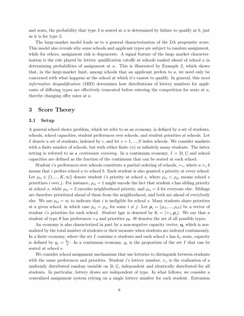
Not surprisingly, a few significant imbalances emerge in balance tests for the longer list ofbaseline covariates, reported in Table 6b. Here, the simulated score seems to balance charac-teristics somewhat more completely than does the DA score, but the F-statistics (reported atthe bottom of the table) that jointly test balance of all baseline covariates fail to reject the nullhypothesis of conditional balance for any specification reported.

Baseline score gaps as large as −.1σ appear in some of the comparisons at the bottom of thetable. The fact that these gaps are not mirrored in the comparisons in Table 4 tells suggests thedifferences in Table 6 are due to chance. Still, we can mitigate the effect of chance differences on2SLS estimates of charter effects by adding baseline score controls (and other covariates) to ourempirical models. The inclusion of these additional controls also has the salutary effect of makingthe 2SLS estimates of interest considerably more precise (baseline score controls are responsiblefor most of the resulting precision gain).

Modes of Inference

An important question in this context concerns the appropriate mode of inference when inter-preting statistical results like that reported in tables like 6a and 6b. Econometric inferencetypically tries to quantify the uncertainty due to random sampling. Here, we might imaginethat the 2012 DPS applicants we happen to be studying constitute a random sample from somelarger population or stochastic process. At the same time, its clear that the uncertainty in ourempirical work can also be seen as a consequence of random assignment : we see only a singlelottery draw for each applicant, one of many possibilities. The population of 2012 applicants, onthe other hand, is fixed, and therefore not a source of uncertainty.

In an effort to determine whether the distinction between sampling inference and random-ization inference matters for our purposes, we computed randomization p-values by repeatedlydrawing lottery numbers and calculating offer gaps in covariates conditional on the simulatedpropensity score. Conditioning on the simulated score produces near-perfect balance in Table 4so this produces an appropriate null distribution. Randomization p-values are given by quantilesof the t-statistics in the distribution resulting from these repeated draws.

14Table 6 reports the results controlling for frequency estimates of the DA propensity score and the simulatedpropensity score. Balance results using formula estimates of the score appear in Appendix Table B3.

23

The p-values associated with the t-statistics for covariate balance computed from the real-ized DPS data turn out to be close to the randomization p-values (for the number of charterschools ranked, for example, the conventional p-value for balance is 0.885 while the correspondingsampling p-value is 0.850). This is consistent with the the theorem from mathematical statisticswhich says that randomization and sampling p-values for differences in means are asymptoticallyequivalent (see Lehmann and Romano 2005 chapter 15).

Apart from a small simulation error, the simulated score can be seen as a “known” or pop-ulation score. Our empirical strategy conditions on formula and frequency estimates of thepropensity score as well as the known (simulated) score. As noted by Hirano et al. (2003) andAbadie and Imbens (2012), conditioning on an estimated score may affect sampling distributions.We therefore checked conventional large-sample p-values against randomization p-values for thereduced-form charter offer effects associated with the various sorts of 2SLS estimates discussedin the next section. Conventional asymptotic sampling formulas generate p-values close to arandomization-inference benchmark, regardless of how the score behind these estimates was con-structed. In view of these findings, we rely on the usual asymptotic (robust) standard errors andtest statistics for inference about treatment effects.15

4.4 Effects of Charter Enrollment

A DA-generated charter offer boosts charter middle school attendance rates by about 0.4. Thesefirst-stage estimates, computed by estimating equation (4), are reported in the first row of Table7. First stage estimates of around 0.68 computed without score controls, shown in column 4 ofthe table, are clearly biased upwards. These estimates and those that follow are from models thatalso control for baseline test scores and a few other covariates described in a footnote. The extracontrols are not necessary for consistent causal inference but their inclusion increases precision(Estimates without covariates appear in the appendix).16

2SLS estimates of charter attendance effects on test scores, reported below the first-stageestimates in Table 7, show remarkably large gains in math, with smaller effects on reading. Themath gains reported here are similar to those found for charter students in Boston (see, forexample, Abdulkadiroğlu et al. 2011). Previous lottery-based studies of charter schools likewisereport substantially larger gains in math than in reading. Here, we also see large and statisticallysignificant gains in writing scores.17

15Appendix table B2 reports conditional-on-score estimates of attrition differentials by offer status. Here, wesee marginally significant gaps on the order of 4-5 points when estimated conditional on the DA propensity score.Attrition differentials fall to a statistically insignificant 3 points when estimated conditional on a simulated score.The estimated charter attendance effects discussed below are similar when computed using either type of scorecontrol, so it seems unlikely that differential attrition is a source of bias in our 2SLS estimates.

16Results here are for scores in grades 4-10. The pattern of results in an analysis that separates high schoolsfrom middle and elementary schools is similar. The sample used for IV estimation is limited to charter applicantswith the relevant propensity score in the unit interval, for which score cells have offer variation in the data athand (these restrictions amount to the same thing for the frequency score). The OLS estimation sample includescharter applicants, ignoring score- and cell-variation restrictions. Estimates in this and the following tables alsocontrol for grade tested, gender, origin school charter status, race, gifted status, bilingual status, subsidized pricelunch eligibility, special education, limited English proficient status, and test scores at baseline.

17Standard errors for the 2SLS estimates reported here ignore the fact that the DA propensity score is estimated.

24

Importantly for our methodological agenda, charter impact estimates reported in Table 7 arelargely invariant to whether the propensity score is estimated by simulation or by a frequency orformula calculation that uses Theorem 1. Compare, for example, math impact estimates of 0.496,0.524, and 0.543 using frequency-, formula-, and simulation-based score controls, all estimatedwith similar precision. This alignment validates the use of Theorem 1 to control for applicanttype.

Estimates that omit propensity score controls highlight the risk of selection bias in a naive2SLS empirical strategy. This is documented in column 4 of Table 7, which shows that 2SLSestimates of math and writing effects constructed using DA offer instruments while omittingpropensity score controls are too small by about half. A corresponding set of OLS estimateswithout propensity score controls, reported in column 5 of the table, also comes in too small.The results in column 6 show that adding score controls to the OLS model pulls the estimates upa little, but a substantial gap between between these and the corresponding set of 2SLS estimatesremains.

Finally, an appendix table (B5) compares the 2SLS estimates reported inTable 7 with semi-parametric estimates of average treatment effects constructed using propensity score weightinginstead of additive linear models. The semiparametric estimates are remarkably similar to thecorresponding 2SLS estimates. Compare, for example, frequency-score-controlled 2SLS estimatesof effects on math and reading of 0.496 and 0.127 with semiparametric estimates around 0.44and 0.11, respectively. At the same time, standard errors for the semiparametric estimates aremarkedly higher than those for 2SLS (precision is estimated using a Bayesian bootstrap thatrandomly reweights observations; see (Shao and Tu, 1995) for an introduction).18

This is probably conservative: Abadie and Imbens (2012) show that the correction for conditioning on an estimatedscore reduces the asymptotic variance matrix for an estimated average treatment effect. Strictly speaking, our2SLS procedure estimates a population average treatment effect only under additional assumptions (like constanteffects). Still, as noted in our discussion of modes of inference, the p-values implied by conventional (robust) 2SLSstandard errors ignoring score estimation come out close to randomization p-values, suggesting any adjustmentfor score estimation in this context is small.

18The score weighting estimators are the sample analogs of

1

P [C1i > C0i]× E[(Di − pD(θ))Yi]

E[pθ(1− pD(θ))],

where pD(θ) is the propensity score estimated using frequency or formula, and the first stage, P [C1i > C0i], isestimated two ways. The "Abadie" version uses

E

{1− Ci(1−Di)

1− pD(θ)− (1− Ci)Di

pD(θ)

},

as suggested by (Abadie, 2003). The "Hirano" version uses

E[(Di − pθ)Ci]E[pD(θ)(1− pθ)]

,

as suggested by (Hirano et al., 2003) and paralleling the estimand for the reduced form. See (Angrist andRokkanen, 2015) for details and an application of both estimators.

25

4.5 Alternative Identification Results

We’re interested in comparing 2SLS estimates constructed using a DA offer dummy as an instru-ment while controlling for the DA propensity score with suitably-controlled estimates constructedusing first-choice and qualification instruments. As noted in Section 3.4, we expect DA-offer in-struments to yield a precision gain and to increase the number of schools represented in theestimation sample relative to these two previously-employed IV strategies.19

Let Q(θi) be a variable that uniquely identifies the charter school that applicant i ranks first,along with his priority status at this school, defined for applicants whose first choice is indeeda charter school. Q(θi) ignores other schools that might have been ranked. The first-choicestrategy is implemented by the following 2SLS setup:

Yi =∑x

α(x)qi(x) + βCi + εi, (6)

Ci =∑x

γ(x)qi(x) + δDfi + νi, (7)

where the di(x)’s are dummies indicating values of Q(θi), indexed by x, and γ(x) and α(x)

are the associated “qualification risk set effects” in the first and second stages. The first-choiceinstrument, Df

i , is a dummy variable indicating i’s qualification at his or her first-choice school.In other words,

Dfi = 1[πis ≤ cs for charter s that i has ranked first].

First choice qualification is the same as first choice offer since under DA, applicants who rank afirst are offered a seat there if and only if they qualify at a.

The qualification strategy expands the sample to include all charter applicants, with Q(θi)

identifying the set of all charter schools that i ranks, along with his or her priority status at each ofthese schools. Q(θi) ignores the order in which schools are ranked, coding only their identities, butpriorities are associated with schools.20 The qualification instrument, Dq

i , indicates qualificationat any charter he or she has ranked. In other words,

Dqi = 1[πis ≤ cs for at least one charter s that i has ranked].

In large markets, the instruments Dfi and Dq

i are independent of type conditional on Q(θi); seeAppendix A.4 for details.

A primary source of inefficiency in the first-choice and qualification strategies is apparent inPanel A of Table 8. This panel reports two sorts of first stage estimates for each instrument:the first of these regresses a dummy indicating any charter offer–that is, our DA charter offerinstrument, Di–on each of the three instruments under consideration. A regression of Di on itselfnecessarily produces a coefficient of one. By contrast, a first-choice offer boosts the probability

19First-choice applications include Abdulkadiroğlu et al. (2013), Deming (2011), Deming et al. (2014), andHastings et al. (2009). First-choice instruments have also been used with decentralized assignment mechanisms(Cullen et al. (2006), Abdulkadiroğlu et al. (2011), Dobbie and Fryer (2011), and Hoxby et al. (2009)). Dobbieand Fryer (2014), Lucas and Mbiti (2014), and Pop-Eleches and Urquiola (2013) use qualification instruments.

20For example, an applicant who ranks A and B with marginal priority only at A is distinguished from anapplicant who ranks A and B with marginal priority only at B.

26

of any charter offer by only around 0.77 in the sample of those who’ve ranked a charter first.This reflects the fact that, while anyone receiving a first choice charter offer has surely beenoffered a charter seat, roughly 23% of the sample ranking a charter first is offered a charter seatat schools other than their first choice. The relationship between Dq

i and charter offers is evenweaker, at around 0.48. This reflects the fact that for schools below the one ranked first, charterqualification is not sufficient for a charter offer.

The diminished impact of the two alternative instruments on charter offers translates into aweakened first stage for charter enrollment. The best case scenario, using all DA-generated offers(that is, Di) as a source of quasi-experimental variation, produces a first stage of around 0.41(this differs from the first-stage estimates reported in Table 7 in that it uses a pooled elementary-middle-high-school sample). But first-choice offers boost charter enrollment by just 0.32, whilequalification anywhere yields a charter enrollment gain of only 0.18. As always with comparisonsof IV strategies, the size of the first stage is a primary determinant of relative precision.

At 0.071, the standard error of the DA-offer estimate is markedly lower than the standarderror of 0.102 yielded by a first-choice strategy and well below the standard error of 0.149 gen-erated by qualification instruments. In fact, the precision loss here is virtually the same as thedecline in the intermediate first stages recorded in the first row of the table (compare 0.774 with0.071/0.102 = 0.696 and 0.476 with 0.071/0.149 = 0.477). The loss here is substantial: columns4 and 5 show the sample size increase needed to undo the damage done by a smaller first stagefor each alternative instrument.21

Only half as many schools are represented in the first-choice analysis sample as in the DAsample (At 24, the number of schools in the qualification sample is closer to the full complementof 30 schools available for study with DA offers). First-choice analyses lose schools because manylotteries fail to randomize first-choice applicants (as seen in Table 1). It’s therefore interestingto note that the first-choice estimate of effects on math and reading scores are noticeably largerthan the estimates generated using DA offer and qualification instruments (compare the estimateof 0.5 using DA offers with estimates of 0.6 and 0.41 using first-choice and qualification instru-ments). This finding may reflect an advantage for those awarded a seat at their first choice school(Hastings et al. 2009; Deming 2011; Deming et al. 2014 find a general “first choice advantage” inanalyses of school attendance effects.) By contrast, the DA offer instrument yields an estimandthat’s more representative of the full complement of charter schools in the match.

4.6 Charter School Effects with a Mixed Counterfactual

The 2SLS estimates in Tables 7 and 8 contrast charter outcomes with potential outcomes gen-erated by attendance at a mix of traditional public schools and schools from other non-chartersectors. We’d like to simplify this mix so as to produce something closer to a pure sector-to-sector comparison. Allowance for more than one treatment channel also addresses concernsabout charter-offer-induced changes in counterfactual outcomes that might cause violations ofthe exclusion restriction.

21The sample used to construct the estimates in columns 1-3 of Table 8 is limited to those who have variationin the instrument at hand conditional on the relevant risk sets controls.

27

Our first step in this effort is to describe the distribution of non-charter school choices forapplicants who were and weren’t offered a charter seat in the DPS assignment. We then identifythe distribution of counterfactual (non-charter) school sectors for the group of charter-lotterycompliers. Finally, we use the DA mechanism to jointly estimate causal effects of attendance atschools in different sectors, thereby making the non-charter counterfactual in our 2SLS estimatesmore homogeneous.

The analysis here builds on a categorical variable, Wi, capturing school sector in which i

is enrolled. Important DPS sectors besides the charter sector are traditional public schools,innovation schools, magnet schools, and alternative schools. Innovation and magnet schoolsare managed by DPS. Innovation schools design and implement innovative practices meant toimprove student outcomes (for details and a descriptive evaluation of innovation schools, seeConnors et al. 2013). Magnet schools serve students with particular styles of learning. Alter-native schools serve mainly older students struggling with factors that may prevent them fromsucceeding in a traditional school environment. Smaller school sectors include a single chartermiddle school outside the centralized DPS assignment process (now closed) and a private schoolcontracted to serve DPS students.

The distribution of enrollment sectors for students who do and don’t receive a charter offerare described in the first two columns of Table 9. These columns show a charter enrollmentrate of 87% in the group offered a charter seat, along with substantial but much smaller charterenrollment in the non-offered group.22 Perhaps surprisingly, only around 41% of those notoffered a charter seat enroll in a traditional public schools, with the rest of the non-offeredgroup distributed over a variety of school types. Innovation schools are the leading non-charteralternative to traditional public schools. Innovation schools operate under an innovation planthat waives some provisions of the relevant collective bargaining agreements (for a descriptiveevaluation of these schools, see Connors et al. 2013).23

The sector distribution for non-offered applicants with non-trivial charter risk appears in col-umn 3 of Table 9, alongside the sum of the non-offered mean and a charter-offer treatment effecton enrollment in each sector in column 4. These extended first-stage estimates, computed byputting indicators 1(Wi = j) on the left-hand side of equation (4), control for the DA propensityscore and therefore have a causal interpretation. The number of applicants not offered a seatwho end up in a charter school is higher for those with non-trivial charter offer risk than in thefull applicant sample, as can be seen by comparing columns 3 and 1. The charter enrollment firststage that’s implicit in the column 4-vs-3 comparison matches the first stage in Table 7. Firststages for other sectors show charter offers sharply reduce innovation school enrollment as wellas reducing enrollment in traditional public schools.

The 2SLS estimates reported in Table 7 capture causal effect for charter lottery compliers. We22Applicants unhappy with the offer they’ve receive in the first round of the Denver assignment may apply to

schools individually in a second round. This process produces charter offers for those not offered a charter seatinitially.

23Innovation waivers are subject to approval by the Denver Classroom Teachers Association (which organizesDenver public school teachers’ bargaining unit), and they allow, for example, increased instruction time. DPS in-novation schools appear to have much in common with Boston’s pilot schools, a model examined in Abdulkadiroğluet al. (2011).

28

describe the distribution of school sectors for compliers by defining potential sector enrollmentvariables,W1i andW0i, indexed against charter offers, Di. Potential and observed sector variablesare related by

Wi = W0i + (W1i −W0i)Di.

In the population of charter-offer compliers, W1i = charter for all i: by definition, charter-offercompliers attend a charter school when the DPS assignment offers them the opportunity to do so.Here, we’re interested in E[1(W0i = j)|C1i > C0i], that is, the sector distribution for charter-offercompliers in the scenario where they aren’t offered a charter seat. We refer to this distributionas describing “enrollment destinies” for compliers.

Enrollment destinies are marginal potential outcome distributions for compliers. As shown byAbadie (2002), these are identified by a simple 2SLS estimand. The details of our implementationof this identification strategy follow those in Angrist et al. (2015), with the modification thatinstead of estimating marginal potential outcome densities for a continuous variable, the outcomesof interest here are Bernoulli.24

Column 5 of Table 9 reveals that, among middle- and elementary-school applicants, onlyabout half of charter lottery compliers are destined to end up in a traditional public school ifthey aren’t offered a charter seat. The second most-likely counterfactual destiny for the youngerapplicant group is an innovation school, with nearly a third of non-offered compliers enrollingin one of these. The likelihood of an enrollment destiny outside the charter, traditional, andinnovation sectors is much smaller.

Isolating an Innovation School Effect

The outsize role of innovation schools in counterfactual destinies motivates an empirical strategythat allows for distinct charter and innovation school treatment effects. By pulling innovationschools out of the non-charter counterfactual, we capture charter effects driven mainly by thecontrast between charter and traditional public schools. Comparisons with a more homogeneouscounterfactual also mitigates bias that might arise from violations of the exclusion restriction(discussed in Section 3.4). And, of course, the innovation treatment effect is also of interest inits own right.

For the purposes of this discussion, we code the sector variable, Wi, as taking on the value2 for innovation schools, the value 1 for charters, and 0 otherwise. The corresponding potentialoutcomes are Y2i, Y1i, and Y0i. At this point, we also adopt a constant-effects causal framework;the question of how to identify average causal effects in instrumental variables models withmultiple treatments raises issues that go beyond the scope of this paper.25 Defining constant

24Briefly, our procedure puts (1−Ci)1(Wi = j) on the left hand side of a version of equation (5) with endogenousvariable 1 − Ci. The coefficient on this endogenous variable is an estimate of E[1(W0i = j)|C1i > C0i, Xi]. Thecovariates and sample used here are the same as used to construct the 2SLS impact estimates reported in column1 of Table 7.

25See Behaghel et al. (2013) and Blackwell (2015) for recent progress on this issue.

29

effects with the notation

Y2i − Y0i = β2,

Y1i − Y0i = β1,

our two-sector identification strategy can be motivated by the conditional independence assump-tion,

Y0i ⊥⊥ Zi|θi, (8)

where Zi is a categorical variable that records DA-generated offers in each sector sector (charter,innovation, other).

The instruments here are indicators for charter and innovation-sector offers, D1i = 1[Zi =

1] and D2i = 1[Zi = 2]. These dummy instruments are used in a 2SLS procedure with two

endogenous variables, C1i for charter school enrollment and C2

i for innovation school enrollment.Propensity score conditioning is justified by the fact that conditional independence relation (8)implies

Y0i ⊥⊥ Zi | p1(θ), p2(θ), (9)

where p1(θ) = E[D1i |θ] and p2(θ) = E[D2

i |θ].The 2SLS setup in this case consists of

Yi =∑x

α1(x)d1i (x) +

∑x

α2(x)d2i (x) + β1C

1i + β2C

2i + εi, (10)

C1i =

∑x

γ11(x)d1i (x) +

∑x

γ12(x)d2i (x) + δ11D

1i + δ12D

2i + νi, (11)

C2i =

∑x

γ21(x)d1i (x) +

∑x

γ22(x)d2i (x) + δ21D

1i + δ22D

2i + ηi, (12)

where the dummy control variables, d1i (x) and d2

i (x), saturate estimates of the scores for eachtreatment, p1(θi) and p2(θi), with corresponding score effects denoted by γ’s and α’s in the firstand second stage models. The sample used for this analysis is the union of charter and innovationschool applicants.

As noted by Imbens (2000) and Yang et al. (2014), the key conditional independence rela-tion in this context (equation (9)) suggests we should choose a parameterization that fixes theconditional probability of assignment for all treatment levels jointly. Joint score control replacesthe additive score controls in equations (10), (11), and (12) with score controls of the form

d12i (x1, x2) = 1[p1(θi) = x1, p2(θi) = x2],

where hats denote score estimates and the indices, x1 and x2, run independently over all values inthe support for each score. This model generates far more score fixed effects than does equation(10).26 Fortunately, however, the algebra of 2SLS obviates the need for joint score control;additive is enough.

26When p1(θ) takes on k1 values and p2(θ) takes on k2 values, the additive model has k1+k2−2 score parameters,while the joint model has k1k2 − 1.

30

To see why additive control is adequate for 2SLS models that exploit (9), note first that2SLS estimates of the second stage equation, (10), can be obtained by first regressing each offerdummy on the full set of d1

i (x) and d2i (x) and then using the residuals from this regression as

instruments after dropping these controls from the model (see, e.g., Angrist and Pischke 2009).Note also that both sets of regressors in this auxiliary first-step model are functions of type.A regression of Dj

i on the full set of d1i (x) and d2

i (x) therefore returns fitted values given byE[Dj |θ] = pj(θi).

Suppose now that we replace additive controls, d1i (x) and d2

i (x), with the full set of dummies,d12i (x1, x2), parameterizing the jointly-controlled model. Since the model here is saturated, a

regression of Dji on the full set of d12

i (x1, x2) dummies recovers the conditional expectationfunction of offers given both scores. By the law of iterated expectations, however, this is

E[Dji |p1(θi), p2(θi)] = E{E[Dj

i |θi]|p1(θi), p2(θi)]} = pj(θi).

From this we conclude that the IV equivalent of 2SLS is the same in the additive and jointly-controlled models.27

As a benchmark, columns 1-2 of Table 10 compare charter-only and innovation-only estimatescomputed using DA (frequency) score controls. Each sample is limited to applicants to therelevant sector.28 Like the estimates in Tables 7 and 8, these pool all grades. A parallel set ofsingle-sector estimates using simulated score controls appears in columns 5 and 6. The innovationfirst stage (the effect of an innovation school offer on innovation school enrollment) is around0.35. The pooled single-sector charter estimates in Table 10 are the same as those in Table 7. Notsurprisingly in view of the substantially reduced number of applicants with non-trivial innovationoffer risk (546 in column 2 and 613 in column 6 of Table 10), and the smaller innovation first stage,the innovation attendance effects are relatively imprecise. This imprecision notwithstanding, theinnovation-only model generates a large negative and marginally significant effect on readingwhen estimated with the DA score.

2SLS estimates of equation (10) appear in columns 3 and 7 of Table 10. Charter school effectschange little in this specification, but (insignificant) negative innovation estimates for math flipto positive when estimated using a model that also isolates charter treatment effects. Thenegative innovation school effects on reading seen in columns 2 and 6 also become smaller in thetwo-endogenous-variables models. Most interestingly, perhaps, the marginally significant positivecharter school effect on reading (when estimating using DA score controls) also disappears. Whilecharter students’ reading performance exceeds what we can expect to see were these students toenroll in a mix of traditional and (low-performing) innovation schools, the reading gap betweencharters and traditional public schools is a little smaller.

Finally, as the theoretical discussion above leads us to expect, the results of estimation withjoint score controls, shown in columns 4 and 8 of Table 10, differ little from the estimates

27This conclusion holds in the population, but need not hold exactly in our data (because scores here areestimated by something more elaborate than a sample mean conditional on type) or for models that includeadditional covariates beyond saturated score controls.

28Appendix Table B6 lists innovation schools and describes the random assignment pattern at these schoolsalong the lines of Table 1 for charter schools. Covariate balance and differential attrition results for innovationschools are reported in Appendix Table B7.

31

constructed using additive score controls reported in columns 3 and 7 (a marginally significantthough still imprecisely estimate positive innovation effect on math scores emerges in column4). Overall, it seems fair to say that the findings on charter effectiveness in Table 7 stand whencharter effects are estimated using a procedure that removes the innovation sector from thecharter enrollment counterfactual.

5 Summary and Directions for Further Work

We investigate empirical strategies that use the random tie-breaking embedded in market designsolutions to school matching problems as a research tool. The most important fruit of thisinquiry is the DA propensity score, an easily-computed formula for the conditional probabilityof assignment to particular schools as a function of type. The DA propensity score revealsthe nature of the experimental design generated as a by-product of market design and suggestsdirections in which match parameters might be modified so as to boost the research value ofschool assignment and other matching schemes. We also show how the DA score can be used tosimultaneously evaluate attendance effects in multiple sectors or schools.

A score-based analysis of data from Denver’s unified school match reveals substantial gainsfrom attendance at one of Denver’s many charter schools. The resulting charter effects are similarto those computed using single-school lottery strategies for charters in Boston. At the sametime, as with previously reported results for Boston Pilot schools, Denver’s Innovation modeldoes not appear to generate substantial achievement gains. Our analysis focuses on defining andestimating the DA propensity score, giving less attention to the problem of how best to use thescore for estimation. Still, simple 2SLS procedures seem to work well, and the resulting estimatesof DPS charter effects differ little from those generated by semiparametric alternatives.

The methods developed here should be broadly applicable to markets using the DA familyof mechanisms for centralized assignment. There’s nothing special about markets that matchschools and students, except, perhaps, their accessible high-quality data. At the same time, somemarkets and matches use mechanisms not covered by the DA framework. Most important onthis list is the top trading cycles (TTC) mechanism (Shapley and Scarf, 1974; Abdulkadiroğluand Sönmez, 2003), which allows students to trade priorities rather than treating priorities asfixed. We expect to have theoretical results on the TTC propensity score soon, along withan application to New Orleans Recovery School District, which has experimented with TTCmatching.

Many matching problems, such as the Boston and New York exam schools analyzed byAbdulkadiroğlu et al. (2014), use some kind of non-randomly-assigned tie-breaker rather thana lottery. These schemes embed a regression discontinuity design inside a market design ratherthan a randomized trial. The question of how best to define and exploit a DA propensity scorefor markets that combine regression-discontinuity designs with market design matchmaking isalso a natural next step for our research design and market design agenda.

32

References

Abadie, Alberto, “Bootstrap Tests for Distributional Treatment Effects in Instrumental Vari-able Models,” Journal of the American Statistical Association, 2002, 97(457), 284–292.

, “Semiparametric instrumental variables estimation of treatment response models,” Journalof Econometrics, 2003, 113(2), 231–263.

and Guido Imbens, “Matching on the Estimated Propensity Score,” 2012. Working Paper.

Abdulkadiroglu, Atila and Tayfun Sonmez, “Random Serial Dictatorship and the Core fromRandom Endowments in House Allocation Problems,” Econometrica, 1998, 66(3), 689–701.

Abdulkadiroğlu, Atila and Tayfun Sönmez, “School Choice: A Mechanism Design Ap-proach,” American Economic Review, 2003, 93, 729–747.

, Josh Angrist, and Parag Pathak, “The Elite Illusion: Achievement Effects at Bostonand New York Exam Schools,” Econometrica, 2014, 82(1), 137–196.

, Joshua D. Angrist, Susan M. Dynarski, Thomas J. Kane, and Parag A. Pathak,“Accountability and Flexibility in Public Schools: Evidence from Boston’s Charters and Pilots,”Quarterly Journal of Economics, 2011, 126(2), 699–748.

, Parag A. Pathak, Alvin E. Roth, and Tayfun Sönmez, “Changing the Boston SchoolChoice Mechanism,” 2006. NBER Working paper, 11965.

, Weiwei Hu, and Parag Pathak, “Small High Schools and Student Achievement: Lottery-Based Evidence from New York City,” 2013. NBER Working paper, 19576.

, Yeon-Koo Che, and Yosuke Yasuda, “Expanding “Choice" in School Choice,” AmericanEconomic Journal: Microeconomics, 2015, 7(1), 1–42.

Agarwal, Nikhil and Paulo Somaini, “Demand Analysis Using Strategic Reports: An Ap-plication to a School Choice Mechanism,” 2015. Working Paper.

Ajayi, Kehinde, “Does School Quality Improve Student Performance? New Evidence fromGhana,” 2014. Working paper, Boston University.

Angrist, Joshua D. and Jinyong Hahn, “When to Control for Covariates? Panel Asymptoticsfor Estimates of Treatment Effects,” The Review of Economics and Statistics, 2004, 86(1), 58–72.

and Jörn-Steffen Pischke, Mostly Harmless Econometrics: An Empiricist’s Companion,Princeton University Press, 2009.

and Miikka Rokkanen, “Wanna Get Away? RD Identification Away from the Cutoff,” 2015.Journal of the American Statistical Association, forthcoming.

33

, Guido W. Imbens, and Donald B. Rubin, “Identification of Causal Effects Using Instru-mental Variables,” Journal of the American Statistical Association, 1996, 91(434), 444–455.

, Parag A. Pathak, and Christopher R. Walters, “Explaining Charter School Effective-ness,” American Economic Journal: Applied Economics, 2013, 5(4), 1–27.

, Sarah Cohodes, Susan Dynarski, Parag Pathak, and Christopher Walters, “Standand Deliver: Effects of Boston’s Charter High Schools on College Preparation, Entry, andChoice,” Journal of Labor Economics, 2015, Forthcoming.

Ashlagi, Itai, Yash Kanoria, and Jacob D. Leshno, “Unblanaced Random Matching Mar-kets: the Stark Effect of Competition,” 2015. Working Paper.

Azevedo, Eduardo and Jacob Leshno, “A Supply and Demand Framework for Two-SidedMatching Markets,” 2014. Working Paper.

Azevedo, Eduardo M. and John William Hatfield, “Existence of Stable Matchings in LargeMarkets with Complementarities,” 2015. Working Paper.

Balinski, Michel and Tayfun Sönmez, “A Tale of Two Mechanisms: Student Placement,”Journal of Economic Theory, 1999, 84, 73–94.

Behaghel, Luc, Bruno Crépon, and Marc Gurgand, “Robustness of the EncouragementDesign in a Two-Treatment Randomized Control Trial,” 2013. IZA Discussion Paper No. 7447.

Bergman, Peter, “Educational Attainment and School Desegregation: Evidence from Random-ized Lotteries,” 2014. Working Paper.

Blackwell, Matthew, “Identification and Estimation of Joint Treatment Effects with Instru-mental Variables,” 2015. Working paper, Harvard University.

Bloom, Howard and Rebecca Underman, “Can Small High Schools of Choice Improve Edu-cational Prospects for Disadvantaged Students?,” Journal of Policy Analysis and Management,2014, 33(2).

Budish, Eric, “The Combinatorial Assignment Problem: Approximate Competitive Equilibriumfrom Equal Incomes,” Journal of Political Economy, 2011, 119(6), 1061–1103.

Calsamiglia, Caterina, Chao Fu, and Maia Güell, “Structural Estimation of a Model ofSchool Choices: The Boston Mechanism vs. Its Alternatives,” 2014. Working Paper.

Che, Yeon-Koo and Fuhito Kojima, “Asymptotic Equivalence of Probabilistic Serial andRandom Priority Mechanisms,” Econometrica, 2010, 78(5), 1625–1672.

Connors, Susan, Erika Moldow, Amelia Challender, and Bonnie Walters, “InnovationSchools in DPS: Year Three of an Evaluation Study,” University of Colorado Denver: TheEvaluation Center, School of Education and Human Development, 2013.

34

Cullen, Jullie Berry, Brian A. Jacob, and Steven Levitt, “The Effect of School Choice onParticipants: Evidence from Randomized Lotteries,” Econometrica, 2006, 74(5), 1191–1230.

de Haan, Monique, Pieter A. Gautier, Hessel Oosterbeek, and Bas van der Klaauw,“The Performance of School Assignment Mechanisms in Practice,” 2015. Working Paper.

Deming, David, “Better Schools, Less Crime?,” Quarterly Journal of Economics, 2011, 126(4),2063–2115.

, Justine Hastings, Thomas Kane, and Douglas Staiger, “School Choice, School Qualityand Postsecondary Attainment,” American Economic Review, 2014, 104(3), 991–1013.

Dobbie, Will and Roland G. Fryer, “Exam High Schools and Academic Achievement: Ev-idence from New York City,” American Economic Journal: Applied Economics, 2014, 6(3),58–75.

Dobbie, William and Roland Fryer, “Are High-Quality Schools Enough to Increase Achieve-ment Among the Poor? Evidence from the Harlem Children’s Zone,” American EconomicJournal: Applied Economics, 2011, 3(3), 158–187.

Ergin, Haluk and Tayfun Sönmez, “Games of School Choice under the Boston Mechanism,”Journal of Public Economics, 2006, 90, 215–237.

Gale, David and Lloyd S. Shapley, “College Admissions and the Stability of Marriage,”American Mathematical Monthly, 1962, 69, 9–15.

Hahn, Jinyong, “On the Role of the Propensity Score in Efficient Semiparametric Estimationof Average Treatment Effects,” Econometrica, 1998, 66(2), 315–331.

Hastings, Justine, Christopher Neilson, and Seth Zimmerman, “Are Some DegreesWorth More than Others? Evidence from College Admission Cutoffs in Chile,” 2013. NBERWorking paper 19241.

, Thomas J. Kane, and Douglas O. Staiger, “Heterogenous Preferences and the Efficacyof Public School Choice,” 2009. Working paper, Yale University.

Heckman, James J., Hidehiko Ichimura, and Petra Todd, “Matching As An EconometricEvaluation Estimator,” Review of Economic Studies, 1998, pp. 261–294.

Hirano, Keisuke, Guido Imbens, and Geert Ridder, “Efficient Estimation of AverageTreatment Effects Using the Estimated Propensity Score,” Econometrica, 2003, 71(4), 1161–1189.

Hoxby, Caroline M., Sonali Murarka, and Jenny Kang, “How New York City’s CharterSchools Affect Achievement,” 2009. Working Paper.

Imbens, Guido, “The Role of the Propensity Score in Estimating Dose-response Functions,”Biometrica, 2000, 87(3), 706–710.

35

and Joshua D. Angrist, “Identification and Estimation of Local Average Treatment Effects,”Econometrica, 1994, pp. 467–475.

Immorlica, Nicole and Mohammad Mahdian, “Marriage, Honesty, and Stability,” SODA,2005, pp. 53–62.

Jackson, Kirabo, “Do Students Benefit from Attending Better Schools? Evidence from Rule-based Student Assignments in Trinidad and Tobago,” Economic Journal, 2010, 120(549),1399–1429.

Kesten, Onur, “Why Do Popular Mechanisms Lack Efficiency in Random Environments?,”Journal of Economic Theory, 2009, 144(5), 2209–2226.

and Utku Ünver, “A Theory of School Choice Lotteries,” Theoretical Economics, 2015,10(2), 543–595.

Kirkeboen, Lars, Edwin Leuven, and Magne Mogstad, “Field of Study, Earnings, andSelf-Selection,” 2015. Working Paper.

Kojima, Fuhito and Mihai Manea, “Incentives in the Probabilistic Serial Mechanism,” Jour-nal of Economic Theory, 2010, 145, 106–123.

and Parag A. Pathak, “Incentives and Stability in Large Two-Sided Matching Markets,”American Economic Review, 2009, 99, 608–627.

Lee, SangMok, “Incentive Compatibility of Large Centralized Matching Markets,” 2014. Work-ing Paper.

Lehmann, Erich L. and Joseph P. Romano, Testing Statistical Hypotheses, Springer, 2005.

Lucas, Adrienne and Isaac Mbiti, “Effects of School Quality on Student Achievement: Dis-continuity Evidence from Kenya,” American Economic Journal: Applied Economics, 2014,6(3), 234–63.

Pathak, Parag A. and Jay Sethuraman, “Lotteries in Student Assignment: An EquivalenceResult,” 2010. NBER Working paper 16140.

and Tayfun Sönmez, “Leveling the Playing Field: Sincere and Sophisticated Players in theBoston Mechanism,” American Economic Review, 2008, 98(4), 1636–1652.

Pop-Eleches, Cristian and Miguel Urquiola, “Going to a Better School: Effects and Be-havioral Responses,” American Economic Review, 2013, 103(4), 1289–1324.

Rosenbaum, Paul R., “Model-Based Direct Adjustment,” Journal of the American StatisticalAssociation, 1987, pp. 387–394.

and Donald B. Rubin, “The Central Role of the Propensity Score in Observational Studiesfor Causal Effects,” Biometrica, 1983, pp. 41–55.

36

Roth, Alvin E. and Elliott Peranson, “The Redesign of the Matching Market for AmericanPhysicians: Some Engineering Aspects of Economic Design,” American Economic Review,1999, 89, 748–780.

and Marilda A. O. Sotomayor, Two-sided Matching: a Study in Game-theoretic Modelingand Analysis, Cambridge University Press: Econometric Society monographs, 1990.

Rubin, Donald B. and Neal Thomas, “Matching Using Estimated Propensity Scores: Re-lating Theory to Practice,” Biometrics, 1996, pp. 249–264.

Shao, Jun and Dongsheng Tu, The Jackknife and Bootstrap, Springer, 1995.

Shapley, Lloyd and Herbert Scarf, “On Cores and Indivisibility,” Journal of MathematicalEconomics, 1974, 1, 23–28.

Svensson, Lars-Gunnar, “Strategy-proof Allocation of Indivisible Goods,” Social Choice andWelfare, 1999, 16.

van der Vaart, A. W., Asymptotic Statistics, Cambridge University Press, 2000.

Yang, Shu, Guido Imbens, Zhanglin Cui, Douglas Faries, and Zibgniew Kadziola,“Propensity Score Matching and Subclassification in Observational Studies with Multi-levelTreatments,” 2014. Unpublished manuscript.

37

Figure 1: Propensity Scores and Market Size in in Example 2

Type 3

Type 2

0.833

0.0833

Type 4

0

0.3

0.6

0.9

2 4 6 8 10 12 14 16 18 20 22 24Number of Students of Each Type

Probability of Assignment to School a

Notes: This figure plots finite-market propensity scores for expansions of Example 2 in Section 2.2. For eachvalue of the x axis, we consider an expansion of the example with x students of each type. The propensity scoresplotted here were computed by drawing lottery numbers 100,000 times.

38

Figure 2: Sample Size Gains from the Propensity Score Strategy

025

5010

030

0#

of A

pplic

ants

s.t.

Ran

dom

izat

ion

(Log

Sca

le)

25 50 100 200 300School Capacity (Log Scale)

# of Additional Applicants Subject to Randomization (Log Scale) # of 1st Choice Applicants Subject to Randomization (Log Scale)

Sample Size Gains: Charter Schools

(a)

010

2550

100

200

400

# of

App

lican

ts s

.t. R

ando

miz

atio

n (L

og S

cale

)

10 25 50 100 200 400School Capacity (Log Scale)

# of Additional Applicants Subject to Randomization (Log Scale) # of 1st Choice Applicants Subject to Randomization (Log Scale)

Sample Size Gains: Non Charter Schools

(b)

Notes: These figures compare the sample size under our DA propensity score strategy to that under the firstchoice strategy. Down arrows mean the two empirical strategies produce the same number of applicants subjectto randomization at the corresponding schools. We say a student is subject to randomization at a school if thestudent has the DA propensity score (frequency) of assignment to that school that is neither 0 nor 1.

39

Table 1: DPS charter schoolsPropensity score in (0,1)

School Total applicantsApplicants

offered seatsDA score

(frequency)DA score (formula) Simulated score

Simulated score (first choice)

(1) (2) (3) (4) (5) (6)Elementary and middle schools

Cesar Chavez Academy Denver 62 9 7 9 8 3Denver Language School 4 0 0 0 0 0DSST: Cole 281 129 31 40 44 0DSST: College View 299 130 47 67 68 0DSST: Green Valley Ranch 1014 146 324 344 357 291DSST: Stapleton 849 156 180 189 221 137Girls Athletic Leadership School 221 86 18 40 48 0Highline Academy Charter School 159 26 69 78 84 50KIPP Montbello College Prep 211 39 36 48 55 20KIPP Sunshine Peak Academy 389 83 41 42 44 36Odyssey Charter Elementary 215 6 20 21 22 14Omar D. Blair Charter School 385 114 135 141 182 99Pioneer Charter School 25 5 0 2 2 0SIMS Fayola International Academy Denver 86 37 7 18 20 0SOAR at Green Valley Ranch 85 9 41 42 43 37SOAR Oakland 40 4 0 9 7 2STRIVE Prep - Federal 621 138 170 172 175 131STRIVE Prep - GVR 324 112 104 116 118 0STRIVE Prep - Highland 263 112 2 21 18 0STRIVE Prep - Lake 320 126 18 26 26 0STRIVE Prep - Montbello 188 37 16 31 35 0STRIVE Prep - Westwood 535 141 235 238 239 141Venture Prep 100 50 12 17 17 0Wyatt Edison Charter Elementary 48 4 0 3 2 0

High schoolsDSST: Green Valley Ranch 806 173 290 343 330 263DSST: Stapleton 522 27 116 117 139 96Southwest Early College 265 76 34 47 55 0Venture Prep 140 39 28 42 45 0KIPP Denver Collegiate High School 268 60 29 37 40 24SIMS Fayola International Academy Denver 71 15 6 22 22 0STRIVE Prep - SMART 383 160 175 175 175 175

Notes: This table shows application patterns at charter schools. Column 1 is the number of applicants ranking each school. Columns 3-6 are restricted to applicants with propensity score values that are neither zero (i.e. ineligible for a seat) nor one (i.e. guaranteed a seat) according to different score computation methods. Column 6 is the number of applicants in column 5 who rank each school as their first choice. Elementary and middle schools are those serving grades 4-8. High schools are those serving grades 9 and 10.

Table 2: DA Score anatomyDA Score = 0 DA Score in (0,1) DA Score = 1

Capacity Offers 0≤MID≤1 MID ≥ τs MID = 1 MID < τs 0<MID<1 MID = 0

STRIVE Prep School (1) (2) (3) (4) (5) (6) (7) (8) (9)GVR 324 147 112 0 0 159 0 116 49Lake 274 147 126 0 0 132 0 26 116Highland 244 147 112 0 0 121 0 21 102Montbello 188 147 37 0 0 128 0 31 29Federal 574 138 138 78 284 3 171 1 37Westwood 494 141 141 53 181 4 238 0 18Notes: This table shows how formula scores are determined for STRIVE school seats in grade 6 (all 6th grade seats at these schools are assigned in a single bucket; ineligible applicants, who have a score of zero, are omitted). Column 3 records offers made to these applicants. Columns 4-6 show the number of applicants in partitions with a score of zero. Likewise, columns 7 and 8 show the number of applicants subject to random assignment. Column 9 shows the number of applicants with certain offers.

Eligible applicants

(ρθs > ρs) (ρθs = ρs) (ρθs < ρs) (ρθs < ρs) (ρθs = ρs) (ρθs < ρs) Θ𝑠𝑠𝑛𝑛 Θ𝑠𝑠𝑐𝑐 Θ𝑠𝑠𝑎𝑎 Θ𝑠𝑠𝑐𝑐 Θ𝑠𝑠𝑎𝑎 Θ𝑠𝑠𝑎𝑎

Table 3: Baseline characteristics of DPS studentsPropensity score in (0,1)

DA score (frequency) Simulated scoreAll applicants Enroll at charter All applicants Enroll at charter

(1) (2) (3) (4) (5) (6) (7)Origin school is charter 0.133 0.080 0.130 0.259 0.371 0.230 0.357Female 0.495 0.502 0.518 0.488 0.496 0.506 0.511Race

Hispanic 0.594 0.593 0.633 0.667 0.713 0.636 0.711Black 0.141 0.143 0.169 0.181 0.161 0.192 0.168White 0.192 0.187 0.124 0.084 0.062 0.098 0.059Asian 0.034 0.034 0.032 0.032 0.039 0.033 0.037

Gifted 0.171 0.213 0.192 0.159 0.152 0.165 0.149Bilingual 0.039 0.026 0.033 0.038 0.042 0.032 0.037Subsidized lunch 0.753 0.756 0.797 0.813 0.818 0.800 0.823Limited English proficient 0.285 0.290 0.324 0.343 0.378 0.337 0.380Special education 0.119 0.114 0.085 0.079 0.068 0.083 0.070

Baseline scoresMath 0.000 0.015 0.021 0.037 0.089 0.037 0.062Reading 0.000 0.016 0.005 -0.011 0.007 0.008 -0.002Writing 0.000 0.010 0.006 0.001 0.039 0.016 0.035

N 40,143 10,898 4,964 1,436 828 1,523 781Notes: This table reports demographic characteristics of Denver 3rd-9th graders in 2011-2012, the baseline (and application) year. Column 1 includes all charter and non-charter students. Column 2 restricts the sample to students who submitted an application to the SchoolChoice system for a seat in grades 4-10 at another DPS school in 2012-2013. Column 3 reports values for students ranking any charter school. Columns 4-7 are restricted to applicants with propensity score values that are neither zero (i.e. ineligible for a seat) nor one (i.e. guaranteed a seat). Test scores are standardized to have mean zero and standard deviation one within each grade based on all Denver students.

Denver students

SchoolChoice applicants

Charter applicants

Table 4: Average covariate balance across 400 offer simulationsPropensity score controls

DA score (frequency) Simulated scoreNon-offered

mean No controls Linear Hundredths Saturated Linear HundredthsTen

Thousandths(1) (2) (3) (4) (5) (6) (7) (8)

A. Application covariatesNumber of schools ranked 4.374 -0.340 0.112 0.067 0.054 0.018 0.017 0.001Number of charter schools ranked 1.426 0.474 0.111 0.071 0.056 0.008 0.008 0.002First school ranked is charter 0.290 0.617 0.005 0.005 0.002 0.001 0.001 -0.001

B. Baseline covariatesOrigin school is charter 0.083 0.114 -0.020 -0.005 -0.002 -0.002 -0.002 0.000Female 0.520 -0.007 0.004 0.005 0.005 0.004 0.003 0.000Race

Hispanic 0.595 0.094 -0.010 -0.004 -0.005 0.003 0.001 0.001Black 0.182 -0.031 0.005 0.001 0.002 -0.001 0.001 0.000

Gifted 0.200 -0.021 0.000 -0.001 -0.003 0.003 0.003 0.003Bilingual 0.025 0.020 0.001 0.001 0.001 0.001 0.001 0.001Subsidized lunch 0.767 0.074 0.004 0.003 0.003 0.003 0.000 0.000Limited English proficient 0.289 0.085 -0.001 -0.002 -0.002 0.003 0.001 -0.002Special education 0.087 -0.004 -0.004 -0.005 -0.004 0.000 -0.001 -0.001Baseline scores

Math 0.017 0.010 -0.023 -0.019 -0.020 -0.003 -0.003 0.005Reading 0.034 -0.071 -0.019 -0.017 -0.017 -0.005 -0.004 0.001Writing 0.029 -0.056 -0.019 -0.016 -0.016 -0.002 -0.001 0.003

Average risk set points of support 87 39 47 1,148 51 120Notes: This table shows the average of covariate balance coefficients across 400 charter offer simulations. We first simulate the real Denver mechanism 400 times and run the covariate balance regressions under each simulation. Coefficients are estimated from regressions of each variable on the left on an any-charter simulated offer dummy, controlling for the variables indicated in each column header. Only applicants to 2012-2013 charter seats in grades 4-10 who were enrolled in Denver at baseline grade are included. Test scores are standardized to have mean zero and standard deviation one within each grade based on all Denver students. Charter offer equals one if a student is accepted into any charter school, excluding alternative charters. Column 1 reports baseline characteristics of charter applicants who did not receive a charter offer. For columns 3 and 6, risk set points of support report the average number (across 400 offer simulations) of unique values in the support of the respective propensity scores. For columns 4-5 and 7-8, risk set points of support report the average number of cells (as defined by dummies for each value of the saturated score) with offer instrument variation. Coefficients in columns 3-8 control for the probability of assignment to a charter school according to different functional forms and probability computation methods, and exclude applicants with propensity score equal to zero (i.e. ineligible) or one (i.e. guaranteed). Controls in columns 4 and 7 are dummies for rounded values in the propensity score support, rounding to the hundredths. Controls in column 5 are dummies for every value in the propensity score support. Column 8 are dummies for rounded values of the simulated score, rounding to the ten thousandths.

Table 5: Average covariate balance by market sizeDA score (frequency) controls (saturated)

No controlsActual market

sizeTwice the market

sizeFour times the

market sizeEight times the

market size(1) (2) (3) (4) (5)

Number of schools ranked -0.340 0.054 0.022 0.009 0.003Number of charter schools ranked 0.474 0.056 0.019 0.006 -0.001First school ranked is charter 0.617 0.002 0.001 0.001 0.001

Origin school is charter 0.114 -0.002 0.000 0.001 0.001Female -0.007 0.005 0.001 0.000 0.000Race

Hispanic 0.094 -0.005 0.001 0.003 0.003Black -0.031 0.002 -0.002 -0.002 -0.001

Gifted -0.021 -0.003 -0.002 -0.002 -0.001Bilingual 0.020 0.001 0.001 0.002 0.001Subsidized lunch 0.074 0.003 0.002 0.000 0.000Limited English proficient 0.085 -0.002 0.000 -0.001 -0.002Special education -0.004 -0.004 -0.003 -0.003 -0.002Baseline scores

Math 0.010 -0.020 -0.013 -0.010 -0.009Reading -0.071 -0.017 -0.011 -0.007 -0.005Writing -0.056 -0.016 -0.008 -0.006 -0.006

Average sample size 4,964 1,417 2,631 5,432 11058Notes: This table shows the average of covariate balance coefficients across 400 charter offer simulations using replicas of students in the realized market to increase the market size. Coefficients are estimated from regressions of each variable on the left on an any-charter simulated offer dummy, controlling for the variables indicated in each column header. All estimates are based on a sample of charter applicants to grades 4 through 10 with probability of assignment into a charter school greater than zero and less than one. Average sample size reports the average number of students (across 400 offer simulations) with propensity score values that are neither zero (i.e. ineligible for a seat) nor one (i.e. guaranteed a seat), and whose DA score (frequency) control (saturated) cell has variation in instrument.

Table 6a: Application covariate balancePropensity score controls

DA score (frequency) Simulated score

No controls Linear Hundredths Saturated Linear HundredthsTen

Thousandths(1) (2) (3) (4) (5) (6) (7) (8)

Number of schools ranked -0.341*** 0.097 0.059 0.028 0.014 0.001 -0.061 -0.015(0.046) (0.103) (0.095) (0.094) (0.102) (0.095) (0.125) (0.042)

Number of charter schools ranked 0.476*** 0.143*** 0.100** 0.074 0.020 -0.017 0.009 0.007(0.024) (0.052) (0.047) (0.047) (0.048) (0.043) (0.061) (0.010)

First school ranked is charter 0.612*** 0.012 0.002 -0.001 -0.030 -0.042* 0.012 0.000(0.011) (0.025) (0.022) (0.020) (0.027) (0.022) (0.027) (0.000)

N 4,964 1,436 1,289 1,247 1,523 1,290 681 301

Risk set points of support 88 40 47 1,148 51 126 61

Robust F-test for joint significance 1190 2.70 1.70 1.09 0.49 1.26 0.31 0.34p-value 0.000 0.044 0.165 0.352 0.688 0.287 0.817 0.710

Full applicant type controls

Notes: This table reports coefficients from regressions of the application characteristics on each row on an any-charter school offer receivership dummy. Only applicants to 2012-2013 charter seats in grades 4-10 who were enrolled in Denver at baseline grade are included. Columns 1-7 are as defined in Table 3. Column 8 controls for fully saturated applicant types (that is, unique combinations of applicant preferences over school programs and school priorities in those programs). Robust standard errors are reported in parentheses. P-values for robust joint significance tests are estimated by stacking outcomes and clustering standard errors at the student level.*significant at 10%; **significant at 5%; ***significant at 1%

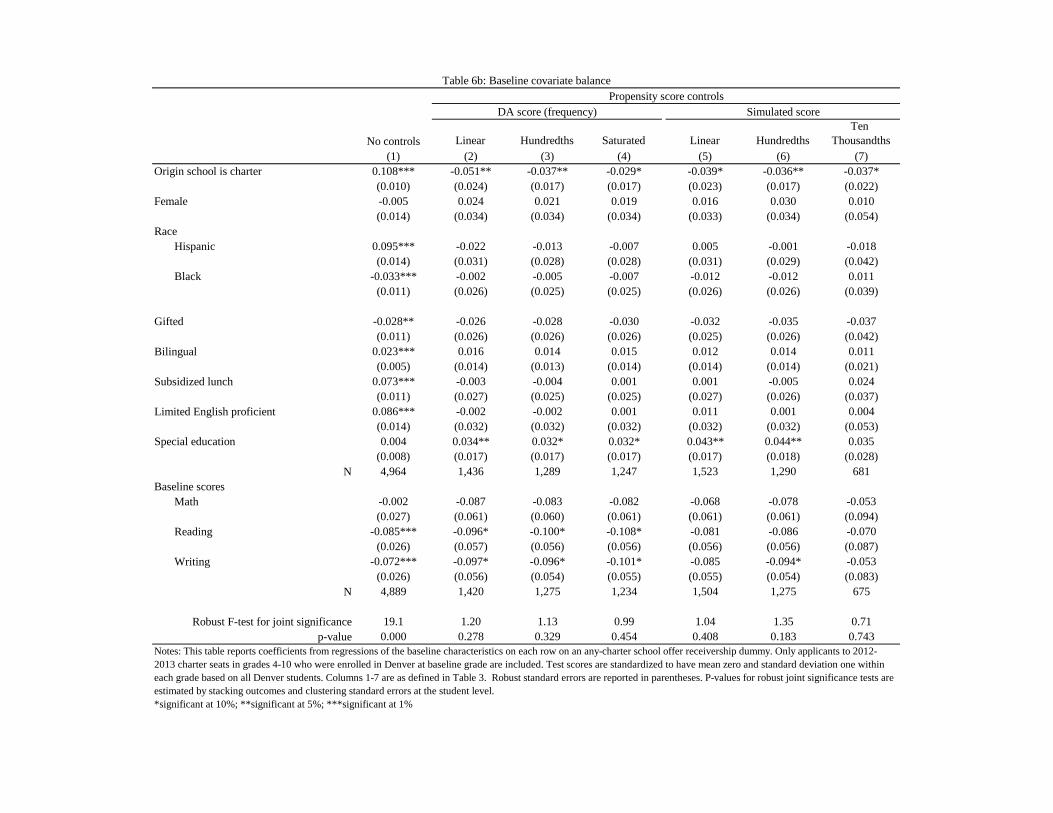
Table 6b: Baseline covariate balancePropensity score controls

DA score (frequency) Simulated score

No controls Linear Hundredths Saturated Linear HundredthsTen

Thousandths(1) (2) (3) (4) (5) (6) (7)

Origin school is charter 0.108*** -0.051** -0.037** -0.029* -0.039* -0.036** -0.037*(0.010) (0.024) (0.017) (0.017) (0.023) (0.017) (0.022)

Female -0.005 0.024 0.021 0.019 0.016 0.030 0.010(0.014) (0.034) (0.034) (0.034) (0.033) (0.034) (0.054)

RaceHispanic 0.095*** -0.022 -0.013 -0.007 0.005 -0.001 -0.018

(0.014) (0.031) (0.028) (0.028) (0.031) (0.029) (0.042)Black -0.033*** -0.002 -0.005 -0.007 -0.012 -0.012 0.011

(0.011) (0.026) (0.025) (0.025) (0.026) (0.026) (0.039)

Gifted -0.028** -0.026 -0.028 -0.030 -0.032 -0.035 -0.037(0.011) (0.026) (0.026) (0.026) (0.025) (0.026) (0.042)

Bilingual 0.023*** 0.016 0.014 0.015 0.012 0.014 0.011(0.005) (0.014) (0.013) (0.014) (0.014) (0.014) (0.021)

Subsidized lunch 0.073*** -0.003 -0.004 0.001 0.001 -0.005 0.024(0.011) (0.027) (0.025) (0.025) (0.027) (0.026) (0.037)

Limited English proficient 0.086*** -0.002 -0.002 0.001 0.011 0.001 0.004(0.014) (0.032) (0.032) (0.032) (0.032) (0.032) (0.053)

Special education 0.004 0.034** 0.032* 0.032* 0.043** 0.044** 0.035(0.008) (0.017) (0.017) (0.017) (0.017) (0.018) (0.028)

N 4,964 1,436 1,289 1,247 1,523 1,290 681Baseline scores

Math -0.002 -0.087 -0.083 -0.082 -0.068 -0.078 -0.053(0.027) (0.061) (0.060) (0.061) (0.061) (0.061) (0.094)

Reading -0.085*** -0.096* -0.100* -0.108* -0.081 -0.086 -0.070(0.026) (0.057) (0.056) (0.056) (0.056) (0.056) (0.087)

Writing -0.072*** -0.097* -0.096* -0.101* -0.085 -0.094* -0.053(0.026) (0.056) (0.054) (0.055) (0.055) (0.054) (0.083)

N 4,889 1,420 1,275 1,234 1,504 1,275 675

Robust F-test for joint significance 19.1 1.20 1.13 0.99 1.04 1.35 0.71p-value 0.000 0.278 0.329 0.454 0.408 0.183 0.743

Notes: This table reports coefficients from regressions of the baseline characteristics on each row on an any-charter school offer receivership dummy. Only applicants to 2012-2013 charter seats in grades 4-10 who were enrolled in Denver at baseline grade are included. Test scores are standardized to have mean zero and standard deviation one within each grade based on all Denver students. Columns 1-7 are as defined in Table 3. Robust standard errors are reported in parentheses. P-values for robust joint significance tests are estimated by stacking outcomes and clustering standard errors at the student level.*significant at 10%; **significant at 5%; ***significant at 1%

Table 7: DPS Charter attendance effects on standardized scores

DA score

(1) (2) (3) (4) (5) (6)First stage 0.410*** 0.389*** 0.377*** 0.683***

(0.031) (0.032) (0.032) (0.012)

Math 0.496*** 0.524*** 0.543*** 0.306*** 0.304*** 0.386***(0.071) (0.076) (0.079) (0.021) (0.015) (0.034)

Reading 0.127** 0.120* 0.106 0.093*** 0.103*** 0.093***(0.065) (0.069) (0.071) (0.020) (0.014) (0.029)

Writing 0.325*** 0.356*** 0.324*** 0.183*** 0.180*** 0.202***(0.077) (0.080) (0.080) (0.023) (0.015) (0.036)

N 1,102 1,083 1,137 4,317 4,317 1,102Notes: This table reports 2SLS and OLS estimates of charter attendance effects on 2012-2013 TCAP scores of Denver 4th-10th graders using the SchoolChoice any-charter offer instrument. Test scores are standardized to have mean zero and standard deviation one within each grade based on all Denver students. Column 6 estimates OLS using DA score (frequency) controls (saturated). Columns 1-6 control for grade tested, gender, origin school charter status, race, gifted status, bilingual status, subsidized price lunch eligibility, special education, limited English proficient status, and test scores at baseline. Robust standard errors are reported in parentheses.*significant at 10%; **significant at 5%; ***significant at 1%

2SLS estimates

Simulated score(hundredths)

Frequency(saturated)

Formula(saturated)

No score controls OLS

OLS with score controls

Table 8: Other IV strategiesCharter attendance effect

(1) (2) (3) (4) (5)A. First stage estimates

1.000 0.774*** 0.476***-- (0.026) (0.024)

0.410*** 0.323*** 0.178***(0.031) (0.035) (0.027)

B. 2SLS estimatesMath 0.496*** 0.596*** 0.409***

(0.071) (0.102) (0.149) 2.0 4.4

Reading 0.127** 0.227** 0.229(0.065) (0.102) (0.144) 2.5 4.9

Writing 0.325*** 0.333*** 0.505***(0.077) (0.119) (0.162) 2.4 4.5

N (students) 1,102 1,125 1,969N (schools) 30 15 24

Notes: This table compares 2SLS attendance effects on 2012-2013 TCAP scores of Denver 4th-10th graders estimated using DA score (frequency) controls (saturated) to other IV strategies. First stage for charter offers reports the regression coefficient of the any-charter offer dummy (the instrument used in column 1) on other instruments, conditioning on the same controls used in the corresponding first stage estimates for charter enrollment. Column 2 reports charter attendance effects using a first-choice charter offer instrument. Column 3 reports charter attendance effects using an any-charter qualification instrument. Columns 2 and 3 control for risk sets making the first-choice and qualification instruments conditionally random; see the main text for details. Columns 2 and 3 exclude 10th graders because there were no 10th grade applicants in risk sets with variation in either first choice offer or any-charter qualification. Test scores are standardized to have mean zero and standard deviation one within each grade based on all Denver students. Columns 4 and 5 report the multiples of the first-choice offer sample size and qualification sample size needed, respectively, in order to achieve a precision gain equivalent to the gain from using the any-charter offer instrument, and is calculated as one minus the square of ratio of the standard error in column 3 to the standard error in column 1. Coefficients in columns 1-3 control for grade tested, gender, origin school charter status, race, gifted status, subsidized price lunch eligibility, special education, bilingual status, limited English proficient status, and test scores at baseline. The last row counts the number of schools for which we observe in-sample variation in the assignment to each school conditional on the cell controls included in the model.*significant at 10%; **significant at 5%; ***significant at 1%

Offer instrument with DA score (frequency) controls (saturated)

First choice charter offer with risk set

controls

Qualification instrument with risk

set controls

Sample size increase for equivalent gain

(col 2 vs col 1)

Sample size increase for equivalent gain

(col 3 vs col 1)

First stage for charter offers

First stage for charter enrollment

Table 9: Enrollment destinies among charter applicantsCharter applicants with DA score (frequency) in (0,1)

All charter applicants All applicants CompliersNo charter offer

(Z = 0)Charter offer

(Z = 1)Non-offered

meanFirst stage

+ col 3No charter offer

(Z = 0)Charter offer

(Z = 1)(1) (2) (3) (4) (5) (6)

Enrolled in a study charter 0.147 0.865 0.347 0.757 -- 1.000 … in a traditional public 0.405 0.081 0.257 0.054 0.497 -- … in an innovation school 0.234 0.023 0.241 0.107 0.328 -- … in a magnet school 0.192 0.021 0.116 0.078 0.094 -- … in an alternative school 0.009 0.005 0.018 0.006 0.030 -- … in a contract school 0.012 0.004 0.018 -0.001 0.047 -- … in a non-study charter 0.001 0.000 0.002 0.000 0.005 --

N 2,555 1,833 498 1,102 -- --Notes: This table describes school enrollment for charter applicants. The sample in this table is identical to that in Table 6. Columns 1-2 describe enrollment for applicants with a charter offer (Z=1) and without a charter offer (Z=0) across all charter applicants, while columns 3-4 and 5-6 show the same for applicants with DA score (frequency) greater than zero and less than one, and for compliers, respectively. Columns 3-6 are restricted to applicants whose DA score (frequency) control (saturated) cells have variation in charter offer. Column 4 adds the non-offered mean in column 3 to the first stage estimate of a regression of a dummy for each school type on the left on an any-charter offer dummy, conditional on the same DA score (frequency) controls and demographic controls as used to construct the estimates in Table 6. School classification is conducted at the grade level, since some schools run magnet programs for a subset of grades served only. Innovation and magnet schools are managed by DPS. Innovation schools design and implement innovative practices to improve student outcomes. Magnet schools serve students with particular styles of learning. Alternative schools include "intensive pathways" and "multiple pathways" schools. The former serve students struggling with academics, behavior, attendance, or other factors that may prevent them from succeeding in a traditional school environment; the latter offer faster pathways toward high school graduation, such as GED preparation and technical education. Non-study charter corresponds to Northeast Academy, a K-8 school that was not included in the SchoolChoice mechanism and closed in May 2013. Contract school corresponds to Escuela Tlatelolco, a private school contracted to serve DPS students. Complier means are estimated by 2SLS following Abadie (2002), using the same DA score (frequency) controls and demographic controls as used to construct the estimates in Table 6. The coefficient for contract school in column 5 was rounded down to zero from -0.002.

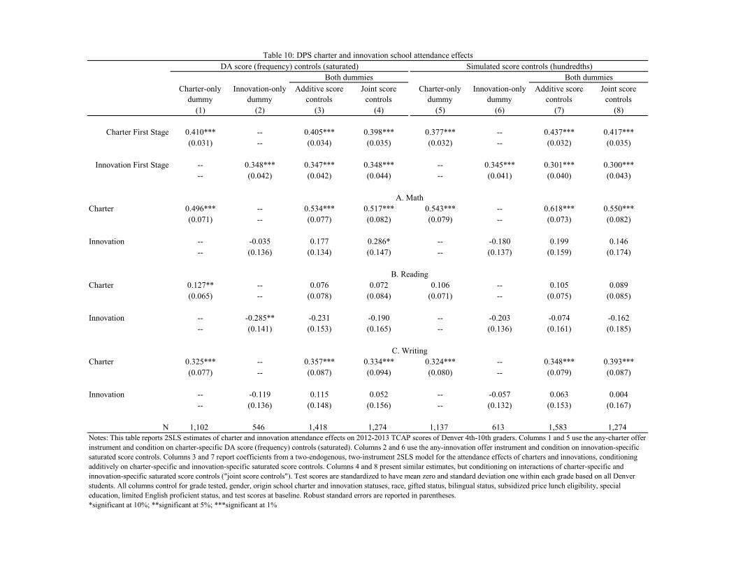
Table 10: DPS charter and innovation school attendance effectsDA score (frequency) controls (saturated) Simulated score controls (hundredths)

Both dummies Both dummies

(1) (2) (3) (4) (5) (6) (7) (8)

Charter First Stage 0.410*** -- 0.405*** 0.398*** 0.377*** -- 0.437*** 0.417***(0.031) -- (0.034) (0.035) (0.032) -- (0.032) (0.035)

Innovation First Stage -- 0.348*** 0.347*** 0.348*** -- 0.345*** 0.301*** 0.300***-- (0.042) (0.042) (0.044) -- (0.041) (0.040) (0.043)

A. MathCharter 0.496*** -- 0.534*** 0.517*** 0.543*** -- 0.618*** 0.550***

(0.071) -- (0.077) (0.082) (0.079) -- (0.073) (0.082)

Innovation -- -0.035 0.177 0.286* -- -0.180 0.199 0.146-- (0.136) (0.134) (0.147) -- (0.137) (0.159) (0.174)

B. ReadingCharter 0.127** -- 0.076 0.072 0.106 -- 0.105 0.089

(0.065) -- (0.078) (0.084) (0.071) -- (0.075) (0.085)

Innovation -- -0.285** -0.231 -0.190 -- -0.203 -0.074 -0.162-- (0.141) (0.153) (0.165) -- (0.136) (0.161) (0.185)

C. WritingCharter 0.325*** -- 0.357*** 0.334*** 0.324*** -- 0.348*** 0.393***

(0.077) -- (0.087) (0.094) (0.080) -- (0.079) (0.087)

Innovation -- -0.119 0.115 0.052 -- -0.057 0.063 0.004-- (0.136) (0.148) (0.156) -- (0.132) (0.153) (0.167)

N 1,102 546 1,418 1,274 1,137 613 1,583 1,274Notes: This table reports 2SLS estimates of charter and innovation attendance effects on 2012-2013 TCAP scores of Denver 4th-10th graders. Columns 1 and 5 use the any-charter offer instrument and condition on charter-specific DA score (frequency) controls (saturated). Columns 2 and 6 use the any-innovation offer instrument and condition on innovation-specific saturated score controls. Columns 3 and 7 report coefficients from a two-endogenous, two-instrument 2SLS model for the attendance effects of charters and innovations, conditioning additively on charter-specific and innovation-specific saturated score controls. Columns 4 and 8 present similar estimates, but conditioning on interactions of charter-specific and innovation-specific saturated score controls ("joint score controls"). Test scores are standardized to have mean zero and standard deviation one within each grade based on all Denver students. All columns control for grade tested, gender, origin school charter and innovation statuses, race, gifted status, bilingual status, subsidized price lunch eligibility, special education, limited English proficient status, and test scores at baseline. Robust standard errors are reported in parentheses.*significant at 10%; **significant at 5%; ***significant at 1%

Charter-only dummy

Innovation-only dummy

Additive scorecontrols

Charter-only dummy

Innovation-only dummy

Additive score controls

Joint score controls

Joint score controls

A Theory Appendix

A.1 Defining DA: Details

Our general formulation defines the DA allocation as determined by cutoffs found in the limit ofa sequence. Recall that these cutoffs evolve according to

ct+1s =

{K + 1 if F (Qs(c

t)) < qs,

max{x ∈ [0,K + 1] | F ({i ∈ Qs(ct) such that πis ≤ x}) ≤ qs

}otherwise,

where Qs(ct) is the demand for seats at school s for a given vector of cutoffs ct and is defined as

Qs(ct) = {i ∈ I | πis ≤ cts and s �i s for all s ∈ S such that πis ≤ cts}.

The following result confirms that these limiting cutoffs exist, i.e., that the sequence ct converges.

Proposition 1. Consider an economy described by a distribution of students F and school capac-ities as defined in Section 3.1. Construct a sequence of cutoffs, cts, for this economy as describedabove. Then, limt→∞ c

ts exists.

Proof. cts is well-defined for all t ≥ 1 and all s ∈ S since it is either K + 1 or the maximizer ofa continuous function over a compact set. We will show by induction that {cts} is a decreasingsequence for all s.

For the base case, c2s ≤ c1

s for all s since c1s = K + 1 and c2

s ≤ K + 1 by construction.For the inductive step, suppose that cts ≤ ct−1

s for all s and all t = 1, ..., T. For each s, ifcTs = K + 1, then cT+1

s ≤ cTs since cts ≤ K + 1 for all t by construction. Otherwise, suppose tothe contrary that cT+1

s > cTs . Since cTs < K + 1, F ({i ∈ Qs(cT−1) such that πis ≤ cTs }) = qs.Then,

F ({i ∈ Qs(cT ) such that πis ≤ cT+1s })

= F ({i ∈ Qs(cT ) such that πis ≤ cTs }) + F ({i ∈ Qs(cT ) such that cTs < πis ≤ cT+1s })

≥ F ({i ∈ Qs(cT−1) such that πis ≤ cTs }) + F ({i ∈ Qs(cT ) such that cTs < πis ≤ cT+1s }) (13)

≥ qs + F ({i ∈ Qs(cT ) such that cTs < πis ≤ cT+1s }) (14)

> qs. (15)

Expression (13) follows because

{i ∈ Qs(cT ) such that πis ≤ cTs }= {i ∈ I | πis ≤ cTs and s �i s for all s ∈ S such that πis ≤ cTs }⊇ {i ∈ I | πis ≤ cTs and s �i s for all s ∈ S such that πis ≤ cT−1

s } (by cTs ≤ cT−1s )

= {i ∈ Qs(cT−1) such that πis ≤ cTs }.

Expression (14) follows by the inductive assumption and since cTs < K + 1.Expression (15) follows since if F ({i ∈ Qs(cT ) such that cTs < πis ≤ cT+1

s }) = 0, then

F ({i ∈ Qs(cT−1) such that πis ≤ cT+1s }) = F ({i ∈ Qs(cT−1) such that πis ≤ cTs }) ≤ qs,

51

while cT+1s > cTs , contradicting the definition of cTs .

Expression (15) contradicts the definition of cT+1 since the cutoff at step T + 1 results inan allocation that exceeds the capacity of school s. This therefore establishes the inductive stepthat cT+1

s ≤ cTs .To complete the proof of the proposition, observe that since {cts} is a decreasing sequence in

the compact interval [0,K + 1], cts converges by the monotone convergence theorem.

Note that this result applies to the cutoffs for both finite and continuum economies. In finitemarkets, at convergence, these cutoffs produce the allocation we get from the usual definition ofDA (e.g., as in Gale and Shapley (1962)). This can be seen by noting that

max{x ∈ [0,K + 1] | F ({i ∈ Qs(ct) such that πis ≤ x}) ≤ qs}= max{x ∈ [0,K + 1] | |{j ∈ Qs(ct) : πjs ≤ x}| ≤ ks},

implying that the tentative cutoff at school s in step t in our DA formulation, which is determinedby the left hand side of this equality, is the same as that in Gale and Shapley (1962)’s DAformulation, which is determined by the right hand side of the equality. Our DA formulationand the Gale and Shapley (1962) formulation therefore produce the same cutoff at each step.This also implies that, in finite markets, our DA cutoffs are found in a finite number of iterations,since DA as described by Gale and Shapley (1962) converges in a finite number of steps.

A.2 Proof of Theorem 1

Admissions cutoffs c in a continuum economy are invariant to lottery outcomes (ri): DA in thecontinuum depends on (ri) only through F (I0) for sets I0 = {i ∈ I | θi ∈ Θ0} with various choicesof Θ0. In particular, F (I0) doesn’t depend on lottery realizations. Likewise, marginal priorityρs is uniquely determined for every school s.

Consider the propensity score for school s. If student i does not rank s, i.e. θi ∈ (Θ\Θs),

then he is not assigned s. Every student of type θ ∈ Θns is not assigned s because ρθs > ρs.

Therefore ps(θ) = 0 for every θ ∈ Θns ∪ (Θ\Θs).

Students of type θ ∈ Θas ∪ Θc

s may be assigned s ∈ Mθs. The ratio of type θ students thatare assigned some s ∈ Mθs is given by MIDθs since lottery numbers are distributed uniformlyrandomly, an assumption that we will use repeatedly in this proof without referring to it. Inother words, the probability of not being assigned any s ∈Mθs for a type θ student is 1−MIDθs.

Every student of type θ ∈ Θas who is not assigned a higher choice is assigned s because ρθs < ρs,

and thereforeps(θ) = (1−MIDθs) for all θ ∈ Θa

s .

Finally, consider students of type θ ∈ Θcs who are not assigned a higher choice. The fraction

of students θ ∈ Θcs who are not assigned a higher choice is 1−MIDθs. Also, the random numbers

of these students is larger than MIDθs. If τs < MIDθs, then no such student is assigned s. Ifτs ≥MIDθs, then the ratio of students that are assigned s within this set is given by τs−MIDθs

1−MIDθs.

Hence, conditional on θ ∈ Θcs and not being assigned a choice higher than s, the probability of

52

being assigned s is given by max{0, τs−MIDθs1−MIDθs

}. Therefore,

ps(θ) = (1−MIDθs)×max

{0,τs −MIDθs

1−MIDθs

}for all θ ∈ Θc

s.

A.3 Proof of Theorem 2

We complete the proof of Theorem 2 in Section 3.3 by proving the following two intermediateresults.

Lemma 1. (Cutoff almost sure convergence) cna.s.−→ c.

Lemma 2. (Propensity score almost sure convergence) For all θ ∈ Θ and s ∈ S, pns(θ)a.s.−→ ps(θ).

A.3.1 Proof of Lemma 1

We use the Extended Continuous Mapping Theorem (Theorem 19.1 in van der Vaart (2000))to prove the lemma. We first show deterministic convergence of cutoffs in order to verify theassumptions of the theorem.

Modify the definition of F to describe the distribution of lottery numbers as well types: Forany set of student types Θ0 ⊂ Θ and for any numbers r0, r1 ∈ [0, 1] with r0 < r1, define the setof students of types in Θ0 with random numbers worse than r0 and better than r1 as

I(Θ0, r0, r1) = {i ∈ I | θi ∈ Θ0, r0 < ri ≤ r1}. (16)

In a continuum economy,

F (I(Θ0, r0, r1)) = E[1{θi ∈ Θ0}]× (r1 − r0),

where the expectation is assumed to exist. In a finite economy with n students,

F (I(Θ0, r0, r1)) =|I(Θ0, r0, r1)|

n.

Let F be the set of possible F ’s defined above. For any two distributions F and F ′, the supnormmetric is defined by

d(F, F ′) = supΘ0⊂Θ,r0,r1∈[0,1]

|F (I(Θ0, r0, r1))− F ′(I(Θ0, r0, r1))|.

The notation is otherwise as in the text.

Proof. Consider a sequence of economies described by a sequence of distributions {fn} overstudents, together with associated school capacities, so that for all n, fn ∈ F is a potentialrealization produced by randomly drawing n students and their lottery numbers from F . Assumethat fn → F in metric space (F , d). Let cn denote the admissions cutoffs in fn. Note the cn isconstant because this is the cutoff for a particular realized economy fn.

The proof first shows deterministic convergence of cutoffs for any convergent subsequenceof fn. Let {fn} be a subsequence of realized economies {fn}. The corresponding cutoffs aredenoted {cn}. Let c ≡ (cs) be the limit of cn. The following two claims establish that cn → c,the cutoff associated with F .

53

Claim 1. cs ≥ cs for every s ∈ S.

Proof of Claim 1. This is proved by contradiction in 3 steps. Suppose to the contrary thatcs < cs for some s. Let S′ ⊂ S be the set of schools the cutoffs of which are strictly lowerunder c. For any s ∈ S′, define Isn = {i ∈ I|cns < πis ≤ cs and i ranks s first} where I is theset of students in F , which contains the set of students in fn for all n. In other words, Isnare the set of students ranking school s first who have a student rank in between cns and cs.

Step (a): We first show that for our subsequence, when the market is large enough, theremust be some students who are in Isn. That is, there exists N such that for any n > N , wehave fn(Isn) > 0 for all s ∈ S′.

To see this, we begin by showing that for all s ∈ S′, there exists N such that for any n > N ,we have F (Isn) > 0. Suppose, to the contrary, that there exists s ∈ S′ such that for all N ,there exists n > N such that F (Isn) = 0. When we consider the subsequence of realizedeconomies {fn}, we find that

fn({i ∈ Qs(cn) such that πis ≤ cs})= fn({i ∈ Qs(cn) such that πis ≤ cns}) + fn({i ∈ Qs(cn) such that cns < πis ≤ cs})= fn({i ∈ Qs(cn) such that πis ≤ cns}) (17)

≤ qs. (18)

Expression (17) follows from Assumption 1 by the following reason. (17) does not hold, i.e.,fn({i ∈ Qs(cn) such that cns < πis ≤ cs}) > 0 only if F ({i ∈ I|cns < πis ≤ cs}) > 0.This and Assumption 1 imply F ({i ∈ I|cns < πis ≤ cs and i ranks s first}) ≡ F (Isn) > 0, acontradiction to F (Isn) = 0. Since fn is realized as n iid samples from F , fn({i ∈ I|cns <πis ≤ cs}) = 0. Expression (18) follows by our definition of DA, which can never assign morestudents to a school than its capacity for each of the n samples. We obtain our contradictionsince cns is not maximal at s in fn since expression (18) means it is possible to increase thecutoff cns to cs without violating the capacity constraint.

Given that we’ve just shown that for each s ∈ S′, F (Isn) > 0 for some n, it is possible tofind an n such that F (Isn) > ε > 0. Since fn → F and so fn → F , there exists N suchthat for all n > N , we have fn(Isn) > F (Isn) − ε > 0. Since the number of schools is fi-nite, such N can be taken uniformly over all s ∈ S. This completes the argument for Step (a).

Step (a) allows us to find some N such that for any n > N , fn(Isn) > 0 for all s′ ∈ S′. Letsn ∈ S and t be such that ct−1

ns ≥ cs for all s ∈ S and ctnsn < csn . That is, sn is one of thefirst schools the cutoff of which falls strictly below csn under the DA algorithm in fn, whichhappens in round t of the DA algorithm. Such sn and t exist since the choice of n guaranteesfn(Isn) > 0 and so cns < cs for all s ∈ S′.

54

Step (b): We next show that there exist infinitely many values of n such that the associatedsn is in S′ and fn(Isn) > 0 for all s ∈ S′. It is because otherwise, by Step (a), there exists Nsuch that for all n > N , we have sn 6∈ S′. Since there are only finitely many schools, {sn}has a subsequence {sm} such that sm is the same school outside S′ for all m. By definitionof sn, cmsm ≤ ctmsm < csm for all m and so csm < csm , a contradiction to sm 6∈ S′. Therefore,we have our desired conclusion of Step (b).

Fix some n such that the associated sn is in S′ and fn(lsn) > 0 for all s ∈ S′. Step (b)guarantees that such n exists. Let Ansn and Asn be the sets of students assigned sn underfn and F, respectively. All students in I snn are assigned sn in F and rejected by sn in fn.

Since these students rank sn first, there must exist a positive measure (with respect to fn)of students outside I snn who are assigned sn in fn and some other school in F ; denote the setof them by Ansn\Asn . fn(Ansn\Asn) > 0 since otherwise, for any n such that Step (b) applies,

fn(Ansn) ≤ fn(Asn \ I snn ) = fn(Asn)− fn(I snn ),

which by Step (a) converges to something strictly smaller than F (Asn) sincefn(Asn) → F (Asn) and fn(I snn ) > 0 for all large enough n by Step (a). Note thatF (Asn) is weakly smaller than qsn . This implies that for large enough n, fn(Ansn) < qsn , acontradiction to Ansn ’s being the set of students assigned sn at a cutoff strictly smaller thanthe largest possible value K + 1. For each i ∈ Ansn \ Asn , let si be the school to which i isassigned under F .

Step (c): To complete the argument for Claim 1, we show that some i ∈ Ansn \ Asn musthave been rejected by si in some step t ≤ t − 1 of the DA algorithm in fn. That is, thereexists i ∈ Ansn \Asn and t ≤ t− 1 such that πisi > ctnsi . Suppose to the contrary that for alli ∈ Ansn \ Asn and t ≤ t − 1, we have πisi ≤ ctnsi . Each such student i must prefer si to snbecause i is assigned si 6= sn under F though πisn ≤ cnsn < csn , where the first inequalityholds because i is assigned sn in Fn while the second inequality does because sn ∈ S′. Thisimplies none of Ansn \Asn is rejected by si, applies for s, and contributes to decreasing ctnsnat least until step t and so ctnsn < csn cannot be the case, a contradiction. Therefore, wehave our desired conclusion of Step (c).

Claim 1 can now be established by showing that Step (c) implies there are i ∈ Ansn \ Asnand t ≤ t − 1 such that πisi > ctnsi ≥ cnsi , where the last inequality is implies by the factthat in every economy, for all s ∈ S and t ≥ 0, we have ct+1

s ≤ cts. Also, they are assigned siin F so that πisi ≤ csi . These imply csi > ctnsi ≥ cnsi . That is, the cutoff of si falls below csiin step t ≤ t− 1 < t of the DA algorithm in fn. This contradicts the definition of sn and t.Therefore cs ≥ cs for all s ∈ S, as desired.

Claim 2. By a similar argument, cs ≤ cs for every s ∈ S.

Since cs ≥ cs and cs ≤ cs for all s, it must be the case that cn → c. The following claim usesthis to show that cn → c.

Claim 3. If cn → c for every convergent subsequence {cn} of {cn}, then cn → c.

55

Proof of Claim 3. Since {cn} is bounded in [0,K + 1]|S|, it has a convergent subsequenceby the Bolzano-Weierstrass theorem. Suppose to the contrary that for every convergentsubsequence {cn}, we have cn → c, but cn 6→ c. Then there exists ε > 0 such that for allk > 0, there exists nk > k such that ||cnk − c|| ≥ ε. Then the subsequence {cnk}k ⊂ {cn}has a convergent subsequence that does not converge to c (since ||cnk − c|| ≥ ε for all k),which contradicts the supposition that every convergent subsequence of {cn} converges toc.

The last step in the proof of Lemma 1 relates this fact to stochastic convergence.

Claim 4. cn → c implies cna.s.−→ c

Proof of Claim 4. This proof is based on two off-the-shelf asymptotic results from mathe-matical statics. First, let Fn be the distribution over I(Θ0, r0, r1)’s generated by randomlydrawing n students from F . Note that Fn is random since is involves randomly drawing nstudents. Fn

a.s.→ F by the Glivenko-Cantelli theorem (Theorem 19.1 in van der Vaart (2000)).Next, since Fn

a.s.→ F and cn → c, the Extended Continuous Mapping Theorem (Theorem18.11 in van der Vaart (2000)) implies that cn

a.s.−→ c, completing the proof of Lemma 1.

A.3.2 Proof of Lemma 2

Proof. Consider any sequence of economies {fn} such that fn ∈ F for all n and fn → F inthe (F , d) metric space. Let pns(θ) be the (finite-market, deterministic) propensity score for aparticular fn. Note that this subtly modifies the definition of pns(θ) from that in the text. Thechange here is that the propensity score for fn is not a random quantity, because economy fn isviewed as fixed.

For Lemma 2, it is enough to show deterministic convergence of this finite-market score, thatis, pns(θ) −→ ps(θ) as fn → F . To see this, let Fn be the distribution over I(Θ0, r0, r1)’s inducedby randomly drawing n students from F . Note that Fn is random and that Fn

a.s.→ F by theGlivenko-Cantelli theorem (Theorem 19.1 in van der Vaart (2000)). Fn

a.s.→ F and pns(θ)→ ps(θ)

allow us to apply the Extended Continuous Mapping Theorem (Theorem 18.11 in van der Vaart(2000)) to obtain pns(θ)

a.s.−→ ps(θ).We prove convergence of pns(θ) −→ ps(θ) as follows. Let cns and cns′ be the random cutoffs

at s and s′, respectively, in fn, and

τθs ≡ cs − ρθs,τθs− ≡ maxs′�θs{cs′ − ρθs′},τnθs ≡ cns − ρθs, andτnθs− ≡ maxs′�θs{cns′ − ρθs′}.

We can express ps(θ) and pns(θ) as follows.

ps(θ) = max{0, τθs − τθs−}pns(θ) = Pn(τnθs ≥ R > τnθs−)

56

where Pn is the probability induced by randomly drawing lottery numbers given fn, and R isany type θ student’s random lottery number distributed according to U [0, 1]. By Lemma 1, withprobability 1, for all ε1 > 0, there exists N1 such that for all n > N1,

|cns′ − cs′ | < ε1 for all s′,

which implies that with probability 1,

|τnθs− − τθs− |=|{cns1 − ρθs1} − {cs2 − ρθs2}|

<

{|{cns1 − ρθs1} − ({cns1 − ρθs2}+ ε1)| if cs2 − ρθs2 ≥ cns1 − ρθs1|{cns1 − ρθs1} − ({cns1 − ρθs2} − ε1)| if cs2 − ρθs2 < cns1 − ρθs1

= ε1

where in the first equality, s1 ≡ arg maxs′�θs{cns′ − ρθs′} and s2 ≡ arg max{cs′ − ρθs′}. Theinequality is by |cns′− cs′ | < ε1 for all s′. For all ε > 0, the above argument with setting ε1 < ε/2

implies that there exists N such that for all n > N ,

pns(θ)

= Pn(τnθs ≥ R > τnθs−})∈ (max{0, τθs − τθs− − ε,max{0, τθs − τθs− + ε)

∈ (ps(θ)− ε, ps(θ) + ε),

where the second-to-last inclusion is because with probability 1, there exists N such that for alln > N such that |τnθs − τθs|, |τnθs− − τθs− | < ε1 and R ∼ U [0, 1]. This means pns(θ) −→ ps(θ),completing the proof of Lemma 2.

A.4 First Choice and Qualification Instruments: Details

Let Dfi be the first choice instrument defined in section 4.5 and let si be i’s first choice school.

The first choice risk set is Q(θi) ≡ (si, ρis).

Proposition 2. In any continuum economy, Dfi is independent of θi conditional on Q(θi).

Proof. In general,Pr(Df

i = 1|θi = θ)

= Pr(πisi ≤ csi |θi = θ)

= Pr(ρisi + ri ≤ csi |θi = θ)

= Pr(ri ≤ csi − ρisi |θi = θ)

= csi − ρisi ,which depends on θi only through Q(θi) because cutoffs are fixed in the continuum..

Let Dqi and Q(θi) be the qualification instrument and the associated risk set defined in section

4.5. The latter is given by the list of schools i ranks and his priority status at each, that is,Q(θi) ≡ (Si, (ρis)s∈Si) where Si is the set of charter schools i ranks.

57

Proposition 3. In any continuum economy, Dqi is independent of θi conditional on Q(θi).

Proof. In general, we havePr(Dq

i = 1|θi = θ)

= Pr(πis ≤ cs for some s ∈ Si|θi = θ)

= Pr(ρis + ri ≤ cs for some s ∈ Si|θi = θ)

= Pr(ri ≤ cs − ρis for some s ∈ Si|θi = θ)

= Pr(ri ≤ maxs∈Si(cs − ρis)|θi = θ)

= maxs∈Si(cs − ρis),which depends on θi only through Q(θi) because cutoffs are fixed in the continuum.

A.5 Extension to a General Lottery Structure

Washington DC, New Orleans, and Amsterdam use DA with multiple lottery numbers, one foreach school (see, for example, de Haan et al. (2015)). Washington, DC uses a version of DA thatuses a mixture of shared and individual school lotteries. This section derives the DA propensityscore for a mechanism with any sort of multiple tie-breaking.

Let a random variable Ris denote student i’s lottery number at school s. Assume that eachRis is drawn from U [0, 1], independently with schools. We consider a general lottery structurewhere Ris 6= Ris′ for some (not necessarily all) s, s′ ∈ S and i ∈ I.

Partition Bθs into m disjoint sets B1θs, ..., B

mθs, so that s′ and s′′ use the same lottery if and

only if s′, s′′ ∈ Bmθs for some m. (Recall Bθs is defined as {s′ ∈ S | s′ �θ s}). Partition Mθs

similarly, so that Mmθs ⊂ Bm

θs for all m. (Recall Mθs is defined as {s ∈ Bθs | ρs = ρθs}). Notethat these partitions are specific to type θ. With single-school lotteries, m simplifies to |Bθs|,the number of schools type θ ranks ahead of s.

Most informative disqualification, MIDmθs, is defined for each m as

MIDmθs ≡

0 if ρθs > ρs for all s′ ∈ Bm

θs,

max{τs | s ∈Mmθs} if ρθs ≥ ρs for all s′ ∈ Bm

θs with at least one equality,1 if ρθs < ρs for some s′ ∈ Bm

θs.

Let m∗ be the value of m for schools in the partition that use the same lottery as s. Denote theassociated MID by MID∗θs. We define MID∗θs = 0 when the lottery at s is unique and thereis no m∗. The following result extends Theorem 1 to a general lottery structure. The proof isomitted.

Theorem 1 (Generalization). For all s and θ in any continuum economy, we have:

Pr[Di(s) = 1|θi = θ] = ps(θ) ≡

0 if θ ∈ Θn

s ,

Πmm=1(1−MIDm

θs) if θ ∈ Θas ,

Πmm=1(1−MIDm

θs)×max

{0,τs −MID∗θs1−MID∗θs

}if θ ∈ Θc

s.

(19)where we also set ps(θ) = 0 when MID∗θs = 1 and θ ∈ Θc

s.

58

Note that in the single tie breaker case, the expression for ps(θ) reduces to that in Theorem 1since m = 1 in that case.

A.6 The Boston (Immediate Acceptance) Mechanism

Studies by Hastings-Kane-Staiger (2009), Hastings-Neilson-Zimmerman (2012), and Deming-Hastings-Kane-Staiger (2013)), among others, use data generated from versions of the Bostonmechanism. Given strict preferences of students and schools, the Boston mechanism is definedas follows:

• Step 1: Each student applies to her most preferred acceptable school (if any). Each schoolaccepts its most-preferred students up to its capacity and rejects every other student.

In general, for any step t ≥ 2,

• Step t : Each student who has not been accepted by any school applies to her most preferredacceptable school that has not rejected her (if any). Each school accepts its most-preferredstudents up to its remaining capacity and rejects every other student.

This algorithm terminates at the first step in which no student applies to a school. Bostonassignments differ DA in that any offer at any step is fixed; students receiving offers cannot bedisplaced later.

This important difference notwithstanding, the Boston mechanism can be represented as aspecial case of DA by redefining priorities as follows:

Proposition 4. (Ergin and Sönmez (2006)) The Boston mechanism applied to (�i)i and (�s)sproduces the same assignment as DA applied to (�i)i and (�∗s)s where �∗s is defined as follows:

1. For k = 1, 2..., {students who rank s k-th} �∗s {students who rank s k + 1-th}

2. Within each category, �∗s ranks the students in the same order as original �s.

This equivalence allows us to construct a Boston propensity score by redefining priorities so thatpriority groups at a given school consists of applicants who (i) share the same original prioritystatus at the school and (ii) give the same rank to the school.

59

B Data Appendix and Additional Empirical Results

B.1 Data Appendix

The Denver Public Schools (DPS) analysis file is constructed using application, school assign-ment, enrollment, demographic, and outcome data provided by DPS for school years 2011-2012and 2012-2013. All files are de-identified, but students can be matched across years and files.Applicant data are from the 2012-2013 SchoolChoice assignment file and test score data are fromthe CSAP (Colorado Student Assessment Program) and the TCAP (Transitional Colorado As-sessment Program) files. The CSAP was discontinued in 2011, and was replaced by the TCAPbeginning with the 2012-2013 school year. Enrollment, demographic, and outcome data areavailable for students enrolled in DPS only; enrollment data are for October.

Applications and assignment: The SchoolChoice file

The 2012-2013 SchoolChoice assignment file contains information on applicants’ preferences overschools (school rankings), school priorities over applicants, applicants’ school assignments (offers)and lottery numbers, a flag for whether the applicant is subject to the family link policy describedin the main text and, if so, to which sibling the applicant is linked. Each observation in theassignment file corresponds to an applicant applying for a seat in programs within schools knownas a bucket.29 Each applicant receives at most one offer across all buckets at a school. Informationon applicant preferences, school priorities, lottery numbers, and offers are used to compute theDA propensity score and the simulated propensity score.

Appendix Table B1 describes the construction of the analysis sample starting from all appli-cants in the 2012-2013 SchoolChoice assignment file. Out of a total of 25, 687 applicants seekinga seat in DPS in the academic year 2012-2013, 5, 669 applied to any charter school seats in grades4 through 10. We focus the analysis on applicants to grades 4 through 10 because baseline gradetest scores are available for these grades only. We further limit the sample to 4, 964 applicantswho were enrolled in DPS in the baseline grade (the grade prior to the application grade) inthe baseline year (2011-2012), for whom baseline enrollment demographic characteristics areavailable.

Enrollment and demographic characteristics

Each observation in the enrollment files describes a student enrolled in a school in a year, andincludes information on grade attended, student sex, race, gifted status, bilingual status, specialeducation status, limited English proficiency status, and subsidized lunch eligibility.30 Demo-

29Since applicants’ rankings are at the school-level but seats are assigned at the bucket level, the SchoolChoiceassignment mechanism translates school-level rankings into bucket-level rankings. For example, if an applicantranked school A first and school B second, and if all seats at both A and B are split into two categories, onefor faculty children (“Faculty”) and one for any type of applicant (“Any”), then the applicant’s ranking of theprograms at A and B would be listed as 10 for Faculty at A, 11 for Any at A, 20 for Faculty at B, 21 for Any atB where numbers code preferences (smaller is more preferred).

30Race is coded as black, white, asian, hispanic, and other. In DPS these are mutually-exclusive categories.

60

graphic and enrollment information are from the first calendar year a student spent in eachgrade.

Applicant outcomes: CSAP/TCAP

Test scores and proficiency levels for the CSAP/TCAP math, reading, and writing exams areavailable for grades 3 through 10. Each observation in the CSAP/TCAP data file correspondsto a student’s test results in a particular subject, grade, and year. For each grade, we use scoresfrom the first attempt at a given subject test, and exclude the lowest obtainable scores as outliers.As a result, 41 observed math scores, 19 observed reading scores, and 1 observed writing scoreare excluded from the sample of charter applicants that are in DPS in baseline year. After outlierexclusion, score variables are standardized to have mean zero and unit standard deviation in asubject-grade-year in the DPS district.

School classification: Parent Guide

We classify schools as charters, traditional public schools, magnet schools, innovation schools,contract schools, or alternative schools (i.e. intensive pathways and multiple pathways schools)according to the 2012-2013 Denver SchoolChoice Parent Guides for Elementary and MiddleSchools and High Schools. School classification is by grade, since some schools run magnetprograms for a few grades only. Schools not included in the Parent Guide (i.e. SIMS FayolaInternational Academy Denver) were classified according to information from the school’s website.

61

Table B1: SchoolChoice application recordsAll applicants In DPS at baseline

Applicants Types Applicants Types(1) (2) (3) (4)

All applicants 25,687 16,087 15,487 9,564Applicants to grades 4 through 10 12,507 7,480 10,898 6,642Applicants to any charters (grades 4 through 10) 5,669 4,833 4,964 4,282Notes: All applications are for the 2012-2013 academic year. Columns 1 and 2 include all applicants in the SchoolChoice assignment file (see Data Appendix for details). Columns 3 and 4 exclude applicants who were not in DPS at the baseline grade (the grade prior to application grade) and baseline year (2011-2012). Applicants to grade "EC" (early childhood, or pre-kindergarten) are excluded from columns 3 and 4 because there is no baseline grade for those applicants. Columns 2 and 4 count unique combinations of applicant preferences over school programs and school priorities in those programs.

Table B2: Differential attritionPropensity score controls

Non-offered mean No controls Linear Hundredths Saturated

Ten Thousandths

(1) (2) (3) (4) (5) (6)A. DA score (frequency)

Enrolls in Denver in follow-up year 0.905 0.029*** 0.041** 0.040** 0.038**(0.008) (0.019) (0.019) (0.019)

Has scores in follow-up year 0.881 0.032*** 0.050** 0.049** 0.048**(0.009) (0.020) (0.020) (0.021)

N 2,939 4,964 1,436 1,289 1,247

B. DA score (formula)Enrolls in Denver in follow-up year 0.905 0.029*** 0.036** 0.027 0.031

(0.008) (0.017) (0.018) (0.020)Has scores in follow-up year 0.881 0.032*** 0.032* 0.026 0.038*

(0.009) (0.018) (0.020) (0.022)

N 2,939 4,964 1,508 1,472 1,224

C. Simulated scoreEnrolls in Denver in follow-up year 0.905 0.029*** 0.037** 0.040** 0.037*

(0.008) (0.018) (0.019) (0.022)Has scores in follow-up year 0.881 0.032*** 0.040** 0.043** 0.046**

(0.009) (0.020) (0.021) (0.023)

N 2,939 4,964 1,523 1,290 1,112Notes: This table reports coefficients from regressions of the availability of follow-up variables on each row on an any-charter school offer receivership dummy. Follow-up variables are observed for academic year 2012-2013. Only applicants to 2012-2013 charter seats in grades 4-10 who were enrolled in Denver at baseline grade are included. Charter offer equals one if a student is accepted into any charter school, excluding alternative charters. Column 1 reports baseline characteristics of charter applicants who did not receive a charter offer. Coefficients in columns 3-6 control for the probability of assignment to a charter school according to different functional forms and probability computation methods, and exclude applicants with propensity score equal to zero (i.e. ineligible) or one (i.e. guaranteed). Controls in column 4 are dummies for rounded values in the propensity score support, rounding to the hundredth. Controls in column 5 are dummies for rounded values of the simulated score, rounding to the thousandth. Controls in column 6 are dummies for every value in the propensity score support. Column 7 controls for fully saturated student types (that is, the profile of all ranked schools and student priorities at the ranked schools). Robust standard errors are reported in parentheses.*significant at 10%; **significant at 5%; ***significant at 1%

Table B3a: Application covariate balanceDA score (formula)

Non-offered mean No controls Linear Hundredths Saturated

(1) (2) (3) (4) (5)Number of schools ranked 4.375 -0.341*** -0.317*** -0.056 -0.001

(0.046) (0.093) (0.086) (0.094)Number of charter schools ranked 1.425 0.476*** 0.062 0.016 0.002

(0.024) (0.043) (0.041) (0.044)First school ranked is charter 0.291 0.612*** 0.003 -0.005 -0.007

(0.011) (0.023) (0.020) (0.019)

N 2,939 4,964 1,508 1,472 1,224

Risk set points of support 156 43 58

Robust F-test for joint significance 1190 8.06 0.47 0.05p-value 0.000 0.000 0.701 0.986

Notes: This table reports coefficients from regressions of the application characteristics on each row on an any-charter school offer receivership dummy. Only applicants to 2012-2013 charter seats in grades 4-10 who were enrolled in Denver at baseline grade are included. Charter offer equals one if a student is accepted into any charter school, excluding alternative charters. For column 3, risk set points of support count unique values in the support of the respective propensity scores. For column 4, risk set points of support count the number of bins or cells (as defined by dummies for each value of the saturated score or as dummies for student types) with offer instrument variation. Column 1 reports baseline characteristics of charter applicants who did not receive a charter offer. Coefficients in columns 3-5 control for the DA score (formula) of being assigned to a charter school according to different functional forms, and exclude applicants with propensity score equal to zero (i.e. ineligible) or one (i.e. guaranteed). Controls in columns 4 are dummies for rounded values in the propensity score support, rounding to the hundredth. Controls in column 5 are dummies for every value in the propensity score support. Robust standard errors are reported in parentheses. P-values for robust joint significance tests are estimated by stacking outcomes and clustering standard errors at the student level.*significant at 10%; **significant at 5%; ***significant at 1%

Table B3b: Baseline covariate balanceDA score (formula)

Non-offered mean No controls Linear Hundredths Saturated

(1) (2) (3) (4) (5)Origin school is charter 0.086 0.108*** 0.085*** -0.012 -0.037**

(0.010) (0.022) (0.017) (0.017)Female 0.520 -0.005 0.014 0.041 0.020

(0.014) (0.030) (0.032) (0.035)Race

Hispanic 0.595 0.095*** -0.004 -0.031 0.003(0.014) (0.028) (0.028) (0.029)

Black 0.183 -0.033*** -0.008 0.008 -0.009(0.011) (0.024) (0.025) (0.027)

Gifted 0.203 -0.028** -0.047** -0.040* -0.036(0.011) (0.023) (0.024) (0.027)

Bilingual 0.289 0.086*** 0.021 -0.002 0.010(0.014) (0.029) (0.030) (0.033)

Subsidized lunch 0.767 0.073*** -0.007 0.011 0.002(0.011) (0.024) (0.023) (0.026)

Limited English proficient 0.289 0.086*** 0.021 -0.002 0.010(0.014) (0.029) (0.030) (0.033)

Special education 0.084 0.004 0.027* 0.036** 0.033*(0.008) (0.016) (0.017) (0.018)

N 2,939 4,964 1,508 1,472 1,224Baseline scores

Math 0.022 -0.002 0.018 -0.049 -0.080(0.027) (0.056) (0.057) (0.063)

Reading 0.040 -0.085*** -0.023 -0.067 -0.100*(0.026) (0.053) (0.053) (0.057)

Writing 0.035 -0.072*** -0.039 -0.068 -0.108*(0.026) (0.051) (0.051) (0.055)

N 2,891 4,889 1,491 1,455 1,213

Robust F-test for joint significance 19.1 2.38 1.16 1.18p-value 0.000 0.005 0.309 0.290

Notes: This table reports coefficients from regressions of the baseline characteristics on each row on an any-charter school offer receivership dummy. Only applicants to 2012-2013 charter seats in grades 4-10 who were enrolled in Denver at baseline grade are included. Test scores are standardized to have mean zero and standard deviation one within each grade based on all Denver students. Charter offer equals one if a student is accepted into any charter school, excluding alternative charters. Column 1 reports baseline characteristics of charter applicants who did not receive a charter offer. Coefficients in column 3-5 control for the DA score (formula) of being assigned to a charter school according to different functional forms, and exclude applicants with propensity score equal to zero (i.e. ineligible) or one (i.e. guaranteed). Controls in columns 4 are dummies for rounded values in the propensity score support, rounding to the hundredth. Controls in column 5 are dummies for every value in the propensity score support. Robust standard errors are reported in parentheses. P-values for robust joint significance tests are estimated by stacking outcomes and clustering standard errors at the student level.*significant at 10%; **significant at 5%; ***significant at 1%

Table B4: DPS Charter attendance effects on standardized scores without covariate controls

DA score

(1) (2) (3) (4) (5) (6)First stage 0.399*** 0.376*** 0.367*** 0.734***

(0.032) (0.032) (0.032) (0.011)

Math 0.339** 0.363** 0.409** 0.239*** 0.285*** 0.457***(0.148) (0.158) (0.162) (0.039) (0.028) (0.067)

Math: Reduced form 0.135** 0.137** 0.150** 0.176***(0.062) (0.063) (0.063) (0.029)

Reading -0.102 -0.108 -0.091 -0.050 0.039 0.158***(0.136) (0.144) (0.150) (0.038) (0.027) (0.059)

Reading: Reduced form -0.041 -0.041 -0.034 -0.037(0.056) (0.056) (0.057) (0.028)

Writing 0.116 0.134 0.140 0.052 0.127*** 0.282***(0.137) (0.144) (0.150) (0.039) (0.027) (0.059)

Writing: Reduced form 0.046 0.051 0.052 0.038(0.057) (0.056) (0.057) (0.028)

N 1,102 1,083 1,137 4,317 4,317 1,102

Frequency(saturated)

Formula(saturated)

Simulation(hundredths)

No score controls OLS

OLS with score controls

Notes: This table reports 2SLS and OLS estimates of charter attendance effects on 2012-2013 TCAP scores of Denver 4th-10th graders using the SchoolChoice any-charter offer instrument. Test scores are standardized to have mean zero and standard deviation one within each grade based on all Denver students. Column 6 estimates OLS using DA score (frequency) controls (saturated). Columns 1-6 control for no covariates but grade tested. Robust standard errors are reported in parentheses.*significant at 10%; **significant at 5%; ***significant at 1%

2SLS estimates

Table B5: Comparison of 2SLS and semiparametric estimates of charter effectsDA score

Frequency (saturated) Formula (saturated)2SLS Abadie Hirano 2SLS Abadie Hirano

(1) (2) (3) (4) (5) (6)

First stage 0.410*** 0.357*** 0.352*** 0.389*** 0.340*** 0.334***(0.032) (0.034) (0.036) (0.031) (0.032) (0.036){0.031} {0.032}

Math 0.496*** 0.437*** 0.443*** 0.524*** 0.478*** 0.486***(0.076) (0.117) (0.120) (0.071) (0.117) (0.119){0.071} {0.076}

Reading 0.127* 0.104 0.106 0.120* 0.116 0.118(0.065) (0.129) (0.131) (0.073) (0.130) (0.132){0.065} {0.069}

Writing 0.325*** 0.322*** 0.326*** 0.356*** 0.359*** 0.364***(0.079) (0.116) (0.119) (0.082) (0.123) (0.127){0.077} {0.080}

N 1,102 1,093 1,093 1,083 1,081 1,081Notes: This table compares 2SLS estimates with estimates computed using semi-parametric propensity score weighting, based on Abadie (2002) and Hirano, Imbens, and Ridder (2003). For details, see Angrist and Rokkanen (2015). Standard errors in parentheses use a Bayesian bootstrap. The table also shows conventional robust standard errors for 2SLS estimates in braces.*significant at 10%; **significant at 5%; ***significant at 1%

Table B6: DPS innovation schoolsPropensity score in (0,1)

School Total applicantsApplicants

offered seatsDA score

(frequency)DA score (formula) Simulated

(1) (2) (3) (4) (5)Elementary and middle schools

Cole Arts and Science Academy 31 15 11 9 10DCIS at Ford 16 0 0 0 1DCIS at Montbello 412 125 163 156 170Denver Green School 153 62 29 46 52Godsman Elementary 10 8 0 0 0Green Valley Elementary 53 15 3 23 35Martin Luther King Jr. Early College 427 177 117 120 121McAuliffe International School 406 165 91 115 112McGlone 14 2 1 4 3Montclair Elementary 15 11 2 1 1Noel Community Arts School 288 108 92 97 105Valdez Elementary 6 3 0 1 1Whittier K-8 School 47 8 1 3 4

High schoolsCollegiate Preparatory Academy 433 125 173 158 153DCIS at Montbello 506 125 208 169 174High-Tech Early College 481 125 209 193 214Manual High School 390 130 152 159 187Martin Luther King Jr. Early College 515 144 179 151 162Noel Community Arts School 334 78 112 112 107

Notes: This table shows application patterns at innovation schools. Column 1 is the number of applicants ranking each school. Columns 3-5 are restricted to applicants with propensity score values that are neither zero (i.e. ineligible for a seat) nor one (i.e. guaranteed a seat) according to different score computation methods. Elementary and middle schools are those serving grades 4-8. High schools are those serving grades 9 and 10.

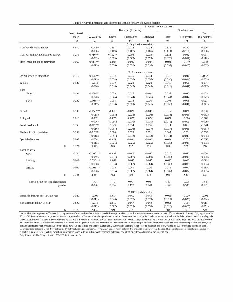
Table B7: Covariate balance and differential attrition for DPS innovation schoolsPropensity score controls

DA score (frequency) Simulated scoreNon-offered

mean No controls Linear Hundredths Saturated Linear HundredthsTen

Thousandths(1) (2) (3) (4) (5) (6) (7) (8)

A. Application covariatesNumber of schools ranked 4.657 -0.142** 0.164 0.012 0.034 0.135 0.132 0.190

(0.058) (0.119) (0.107) (0.106) (0.114) (0.110) (0.158)Number of innovation schools ranked 1.279 0.710*** 0.192** 0.086 0.035 0.121 0.092 0.097

(0.035) (0.079) (0.062) (0.059) (0.076) (0.069) (0.118)First school ranked is innovation 0.052 0.611*** -0.003 -0.007 -0.005 -0.030 -0.030 -0.043

(0.015) (0.036) (0.022) (0.018) (0.032) (0.027) (0.037)

B. Baseline covariatesOrigin school is innovation 0.116 0.125*** 0.032 0.045 0.044 0.010 0.040 0.100*

(0.015) (0.034) (0.036) (0.036) (0.033) (0.034) (0.053)Female 0.526 -0.011 0.030 0.028 0.028 0.063 0.060 0.077

(0.020) (0.046) (0.047) (0.049) (0.044) (0.048) (0.087)Race

Hispanic 0.491 0.136*** 0.028 0.015 -0.001 0.037 0.043 0.039(0.020) (0.045) (0.044) (0.046) (0.044) (0.044) (0.077)

Black 0.262 -0.064*** 0.018 0.018 0.030 0.003 0.009 0.023(0.017) (0.038) (0.039) (0.041) (0.036) (0.040) (0.071)

Gifted 0.198 -0.056*** -0.019 -0.028 -0.041 0.017 0.020 0.008(0.015) (0.034) (0.035) (0.036) (0.033) (0.035) (0.062)

Bilingual 0.018 0.007 -0.025 -0.027* -0.029* -0.020 -0.014 -0.006(0.006) (0.016) (0.016) (0.015) (0.015) (0.015) (0.029)

Subsidized lunch 0.763 0.047*** 0.029 0.034 0.016 0.011 0.013 -0.044(0.016) (0.037) (0.036) (0.037) (0.037) (0.036) (0.061)

Limited English proficient 0.253 0.047*** 0.016 0.032 0.031 0.007 -0.001 -0.030(0.018) (0.041) (0.042) (0.043) (0.041) (0.043) (0.085)

Special education 0.092 0.004 -0.021 -0.031 -0.036 -0.026 -0.037 -0.050(0.012) (0.025) (0.025) (0.025) (0.025) (0.025) (0.062)

N 1,176 2,483 769 717 623 888 705 279Baseline scores

Math -0.017 -0.186*** -0.032 -0.018 -0.057 0.023 0.042 0.030(0.040) (0.091) (0.087) (0.088) (0.088) (0.091) (0.158)

Reading 0.036 -0.220*** -0.066 -0.047 -0.047 -0.013 0.002 0.015(0.038) (0.084) (0.082) (0.084) (0.080) (0.083) (0.153)

Writing 0.000 -0.163*** 0.025 0.041 0.030 0.079 0.081 0.119(0.038) (0.085) (0.082) (0.084) (0.082) (0.084) (0.165)

N 1,158 2,434 752 704 614 869 689 273

Robust F-test for joint significance 143 1.10 0.99 0.91 0.80 0.92 1.52p-value 0.000 0.354 0.457 0.548 0.669 0.535 0.102

C. Differential attritionEnrolls in Denver in follow-up year 0.920 -0.001 -0.017 -0.012 -0.011 -0.015 -0.020 -0.008

(0.011) (0.026) (0.027) (0.029) (0.024) (0.027) (0.044)Has scores in follow-up year 0.897 -0.011 -0.019 -0.014 -0.018 -0.008 -0.017 0.018

(0.012) (0.027) (0.029) (0.030) (0.026) (0.029) (0.051)N 1,176 2,483 769 717 623 888 705 279

Notes: This table reports coefficients from regressions of the baseline characteristics and follow-up variables on each row on an any-innovation school offer receivership dummy. Only applicants to 2012-2013 innovation seats in grades 4-10 who were enrolled in Denver at baseline grade are included. Test scores are standardized to have mean zero and standard deviation one within each grade based on all Denver students. Innovation offer equals one if a student is accepted into any innovation school. Column 1 reports baseline characteristics of innovation applicants who did not receive an innovation offer. Coefficients in columns 3-8 control for the probability of assignment to an innovation school according to different functional forms and probability computation methods, and exclude applicants with propensity score equal to zero (i.e. ineligible) or one (i.e. guaranteed). Controls in columns 4 and 7 group observations into 200 bins of 0.5 percentage-point size each. Coefficients in columns 5 and 8 are estimated by fully saturating propensity score values, with scores in column 8 rounded to the nearest ten-thousandth decimal point. Robust standard errors are reported in parentheses. P-values for robust joint significance tests are estimated by stacking outcomes and clustering standard errors at the student level.*significant at 10%; **significant at 5%; ***significant at 1%