research article the use of fractional order derivative to

Hindawi Publishing CorporationMathematical Problems in EngineeringVolume 2013, Article ID 543026, 9 pageshttp://dx.doi.org/10.1155/2013/543026

Research ArticleThe Use of Fractional Order Derivative toPredict the Groundwater Flow

Abdon Atangana1 and Necdet Bildik2

1 Institute for Groundwater Studies, Faculty of Natural and Agricultural Sciences, University of the Free State,P.O. Box 9300, Bloemfontein, South Africa

2Department of Mathematics, Faculty of Art & Sciences, Celal Bayar University, Muradiye Campus,45047 Manisa, Turkey

Correspondence should be addressed to Abdon Atangana; [email protected]

Received 2 July 2013; Revised 27 August 2013; Accepted 3 September 2013

Academic Editor: Tirivanhu Chinyoka

Copyright © 2013 A. Atangana and N. Bildik. This is an open access article distributed under the Creative Commons AttributionLicense, which permits unrestricted use, distribution, and reproduction in any medium, provided the original work is properlycited.

The aim of this work was to convert the Thiem and the Theis groundwater flow equation to the time-fractional groundwater flowmodel. We first derived the analytical solution of theTheim time-fractional groundwater flow equation in terms of the generalizedWright function. We presented some properties of the Laplace-Carson transform. We derived the analytical solution of the Theis-time-fractional groundwater flow equation (TFGFE) via the Laplace-Carson transform method. We introduced the generalizedexponential integral, as solution of the TFGFE.This solution is in perfect agreement with the data observed from the pumping testperformed by the Institute for Groundwater Study on one of its borehole settled on the test site of the University of the Free State.The test consisted of the pumping of the borehole at the constant discharge rate Q and monitoring the piezometric head for 350minutes.

1. Introduction

Groundwater problem is perhaps one of the most difficultreal-world problems to be modelled into mathematical for-mulation. To model this problem accurately, one must knowprecisely the behavior of the medium through which thewater is moving. However, this medium through which theflow occurs can change from one point to another, alsofrom one period to another. For example, the hydraulicconductivity of an aquifer can differ from one direction toanother. Several scholars have intensively tried to proposea better model that can be used to predict the movementof water through the aquifer. However, their results stillpresent some lacks. Recently, It was revealed that real prob-lems modelled via fractional order derivative present betterresults when matching their mathematical representationwith experimental data. To test this, Botha and Cloot [1]presented some good results by generalizing the groundwaterflow equation to the concept of fractional order derivatives. Inthe same line of ideas, Atangana [2] examined an approximatesolution of the generalized groundwater flow equation via

the Frobenius method. The results obtained from his inves-tigation showed better prediction. Recently, Atangana andBotha further extended the fractional groundwater equationto the concept of the fractional-variation order groundwater[3]. They presented the stability and the convergence of thenumerical scheme via Crank-Nicolson method. Up to now,there is no approximate or exact analytical mathematicalexpression that can be used to describe the solution ofthe fractional groundwater flow equation. Therefore, oneof the purposes of this work is to present some analyticalmathematical expression than can be used as approximatesolution of the time-fractional groundwater flow equation.

An aquifer test (or a pumping test) is conducted to eval-uate an aquifer by “stimulating” the aquifer through constantpumping and observing the aquifer’s “response” (drawdown)in observation wells. Aquifer testing is a common tool thathydrogeologists use to characterize a system of aquifers,aquitards, and flow system boundaries. Aquifer tests aretypically interpreted by using an analytical model of aquiferflow (the most fundamental being the Theis solution) to

2 Mathematical Problems in Engineering

match the data observed in the real-world then assuming thatthe parameters from the idealized model apply to the real-world aquifer. In more complex cases, a numerical modelmay be used to analyze the results of an aquifer test, butadding complexity does not ensure better results. For themost part frequently, an aquifer assessment is carried out bypropelling water out from one borehole at a fixed speed andfor as a minimum of 24 hours at the same time as cautiouslyevaluating the water levels in the observed borehole. Whenwater is pumped from the pumping well, the pressure in theaquifer that feeds that well declines. This decline in pressurewill show up as drawdown (change in hydraulic head) in anobservation well. Drawdown decreases with radial distancefrom the pumping well and drawdown increases with thelength of time that the pumping continues. The aquifercharacteristics which are evaluated by most aquifer tests are[4, 5] as follows.

(i) The hydraulic conductivity is the rate of flow of waterthrough a unit crosses sectional area of an aquifer ata unit hydraulic gradient. In English units the rateof flow is in gallons per day per square foot of crosssectional area.

(ii) Specific storage or storativity being a measure of theamount of water a confined aquifer will give up for acertain change in head.

(iii) The transmissivity is the rate at which water is trans-mitted through a unit thickness of an aquifer undera unit hydraulic gradient. It is equal to the hydraulicconductivity times the thickness of an aquifer.

The rest of this paper has been presented as follows. InSection 1, we presented the background of the fractionalorder derivative. We derived the analytical solution of theTheim fractional groundwater flow equation in Section 3.In Section 4, we presented the derivation of the Theis frac-tional groundwater flow via the Laplace-Carson transformmethod. We presented an alternative analytical solution ofthe Theis fractional groundwater flow equation in termsof the generalized exponential integral in Section 5. Thenumerical comparisons with experimental data are presentedin Section 6 and the conclusion is in Section 7. We will startwith the background of the fractional derivative.

2. Background of the FractionalOrder Derivative

There exists the vast literature on different definitions of frac-tional derivatives. The most popular ones are the Riemann–Liouville and the Caputo derivatives [6–11]. Caputo’s defini-tion has the form of

𝐷𝛼

𝑥(𝑓 (𝑥)) =

1

Γ (𝑛 − 𝛼)

𝑑𝑛

𝑑𝑥𝑛

× ∫

𝑥

0

(𝑥 − 𝑡)𝑛−𝛼−1

𝑓 (𝑡) 𝑑𝑡, 𝑛 − 1 ≤ 𝛼 ≤ 𝑛.

(1)

For the case of the Caputo fractional order derivative, we havethe following definition:

𝐷𝛼

𝑥(𝑓 (𝑥)) =

1

Γ (𝑛 − 𝛼)

× ∫

𝑥

0

(𝑥 − 𝑡)𝑛−𝛼−1

𝑑𝑛

𝑑𝑥𝑛𝑓 (𝑡) 𝑑𝑡, 𝑛 − 1 ≤ 𝛼 ≤ 𝑛.

(2)Each of the pervious fractional order derivatives presentssome advantages and disadvantages [6–10]. The Riemann-Liouville derivative of a constant is not zero while Caputoderivative of a constant is zero but demands higher conditionsof regularity for differentiability [6–10]: to compute thefractional derivative of a function in the Caputo sense, wemust first calculate its derivative [11]. Caputo derivativesare defined only for differentiable functions while functionsthat have no first-order derivative might have fractionalderivatives of all orders less than one in the Riemann-Liouville sense [12, 13]. Guy Jumarie has recentlymodified theRiemann-Liouville derivative (see [14])

𝐷𝛼

𝑥(𝑓 (𝑥))=

1

Γ (𝑛 − 𝛼)

𝑑𝑛

𝑑𝑥𝑛×∫

𝑥

0

(𝑥 − 𝑡)𝑛−𝛼−1

{𝑓 (𝑡)−𝑓 (0)} 𝑑𝑡.

(3)The Caputo fractional derivative will be considered in thiswork due to the applicability of the Caputo derivative in real-world problems [15].

3. Thiem’ Groundwater Flow Equation

The Theim fractional groundwater flow equation is anordinary differential equation given in the following. Theequation describes the change in level of water as functionof distance during the pumping test [5]:

𝐷𝛼

𝑟𝑟Φ (𝑟) +

1

𝑟Φ (𝑟) = 0, 1 < 𝛼 ≤ 2. (4)

Subject to the initial condition, 𝑄 = 2𝜋𝑇𝐷𝑟(Φ(𝑟𝑏)).

We will make use of the Laplace transform to deriveanalytical solution of (4). Thus, multiplying on both sidesof (4) by 𝑟 and secondly applying the Laplace transform, weobtain the following expression:

𝑑 [𝐿 (Φ) (𝑠)]

𝑑𝑠+ (

𝛼

𝑠+

1

𝑠𝛼) (𝐿 (Φ) (𝑠))

=

𝑙

∑

𝑚=2

𝑑𝑚(𝑚 − 1) 𝑠

𝑚−2−𝛼

,

(5)

where 𝑑𝑚= 𝐷𝛼−𝑚

0+ Φ(0

+

) (𝑚 = 2, . . . , 𝑙). Now, one can derivethe solution of the ordinary order differential equation withrespect to the Laplace transform of Θ(𝑠) = 𝐿(Φ(𝑟)):

Θ (𝑠) = 𝑠−𝛼 exp[− 𝑠

1−𝛼

1 − 𝛼]

× [𝑎1+

𝑙

∑

𝑚=2

𝑑𝑚(𝑚 − 1) ∫ 𝑠

𝑚−2 exp[− 𝑠1−𝛼

1 − 𝛼]𝑑𝑠] ,

(6)

Mathematical Problems in Engineering 3

with 𝑎1an arbitrary real constant that will be obtained via the

initial condition.We next expand the exponential function inthe integrand in a series, and using term-by-term integration,we arrive at the following expression:

Θ (𝑠) = 𝑐Θ1(𝑠) +

𝑙

∑

𝑚=2

𝑑𝑚(𝑚 − 1)Θ

∗

𝑚(𝑠) (7)

with, of course,

Θ1(𝑠) = 𝑠

−𝛼 exp[− 𝑠1−𝛼

1 − 𝛼] ,

Θ∗

𝑚(𝑠)=𝑠

−𝛼 exp[ 𝑠1−𝛼

𝛼 − 1]

∞

∑

𝑗=0

(1

1 − 𝛼)

𝑗𝑠(1−𝛼)𝑗+𝑚−1

[(1 − 𝛼) 𝑗 + 𝑚 − 1] 𝑗!.

(8)

Now, applying the inverse Laplace transform on Θ1(𝑠) and

using the fact that

𝑠−[𝛼+(𝛼−1)𝑗]

= 𝐿[𝑟𝛼+(𝛼−1)𝑗−1

Γ (𝛼 + (𝛼 − 1) 𝑗)] (9)

we obtain

Φ1(𝑟) = 𝑟

𝛼−1

𝑜Ψ1[(𝛼, 𝛼 − 1) |

𝑥𝛼−1

𝛼 − 1] (10)

with 𝑜Ψ1[⋅] the generalized Wright function [16] for 𝑝 =

1 and 𝑞 = 2. We next expand the exponential functionexp[−𝑠1−𝛼/(1 − 𝛼)] in power series; multiplying the resultingtwo series; in addition of this if we consider the number𝑏𝑘(𝛼,𝑚) defined for 𝛼 > 0,𝑚 = 2, . . . 𝑙, (𝛼 = (𝑝+𝑚−1)/𝑝, 𝑝 ∉

N) and 𝑘 ∈ N0,

𝑏𝑘(𝛼,𝑚) =

𝑙

∑

𝑝,𝑗=0,...𝑘,𝑝+𝑗=𝑘

(−1)𝑞

𝑝!𝑗! (1 − 𝛼) 𝑞 + 𝑚 − 1. (11)

The previous family of number possesses satisfies the follow-ing recursive formula:

𝑏𝑘(𝛼,𝑚)

𝑏𝑘+1

(𝛼,𝑚)=𝛼 − 𝑚

𝛼 − 1+ 𝑘, (12)

which produces the explicit expression for 𝑏𝑘(𝛼,𝑚) in the

form of

𝑏𝑘(𝛼,𝑚) =

Γ [(𝛼 − 𝑚) / (𝛼 − 1)]

(𝑚 − 1) Γ [((𝛼 − 𝑚) / (𝛼 − 1)) + 𝑘], 𝑘 ∈ N

0.

(13)

Now, having the previous expression on hand, we can derivethat

Θ∗

𝑚(𝑠) = 𝑠

𝑚−𝛼−1

(

∞

∑

𝑗=0

(1

1 − 𝛼)

𝑗𝑠(1−𝛼)𝑝

𝑝!)

× (

∞

∑

𝑝=0

(1

1 − 𝛼)

𝑝(−1)𝑝

[(1 − 𝛼) 𝑝 + 𝑚 − 1]

𝑠(1−𝛼)𝑗

𝑝!)

=

∞

∑

𝑘=0

𝑏𝑘(𝛼,𝑚) (

1

1 − 𝛼)

𝑘

𝑠(1−𝛼)𝑘+𝑚−𝛼−1

(𝑚=2, . . . , 𝑙) .

(14)

However, remembering (9) with 𝛽 = (𝛼 − 1)𝑘 + 𝛼 + 1 −𝑚, wecan further derive the following expression forΦ∗

𝑚(𝑟) as

Φ∗

𝑚(𝑟) =

∞

∑

𝑘=0

𝑏𝑘(𝛼,𝑚) (

1

1 − 𝛼)

𝑘

×Γ (𝑘 + 1)

Γ [𝛼 + 1 − 𝑚 + (𝛼 − 1) 𝑘]

𝑥(𝛼−1)𝑘+𝛼−𝑚

𝑘!

(15)

or in the simplified version we have

Φ∗

𝑚(𝑟) =

Γ [(𝛼 − 𝑚) / (𝛼 − 1)]

(𝑚 − 1)Φ𝑚(𝑟) , (16)

where

Φ𝑚(𝑟) = 𝑟

𝛼−𝑚

1Ψ2

× [

(1, 1)

(𝛼 + 1 − 𝑚, 𝛼 − 1) , (𝛼 − 𝑚

𝛼 − 1, 1)

|𝑟𝛼−1

𝛼 − 1] .

(17)

It follows that the solution of the fractional-Thiem ground-water flow equation is in the form of

Φ (𝑟) = 𝑎1𝑟𝛼−1

𝑜Ψ1[(𝛼, 𝛼 − 1) |

𝑥𝛼−1

𝛼 − 1]

+ 𝑎2

𝑙

∑

𝑚=2

𝑏𝑚(𝑚 − 1)

Γ [(𝛼 − 𝑚) / (𝛼 − 1)]

(𝑚 − 1)𝑟𝛼−𝑚

×1Ψ2[

(1, 1)

(𝛼 + 1 − 𝑚, 𝛼 − 1) , (𝛼 − 𝑚

𝛼 − 1, 1)

|𝑟𝛼−1

𝛼 − 1] .

(18)

In our case 𝑙 = 2.

4. Time-Fractional Theis GroundwaterFlow Equation

The easiest sweeping statement of subsurface water flowequation, which while we are on the subject is in additionin harmony in the midst of the real physics of the observedfact, is to presume that water level is not in a balancedstate but momentary state. Theis (1935) [17] was the first todevelop a formula for unsteady-state flow that introducesthe time factor and the storativity. He noted that when awell-penetrating extensive confined aquifer is pumped at aconstant rate, the influence of the discharge extends outwardwith time. The rate of decline of head, multiplied by thestorativity and summed over the area of influence, equals thedischarge. The unsteady-state (orTheis) equation, which wasderived from the analogy between the flow of groundwaterand the conduction of heat, is perhaps the most widely usedpartial differential equation in groundwater investigations:

𝑆𝐷𝑡Φ (𝑟, 𝑡) = 𝑇𝐷

𝑟𝑟Φ (𝑟, 𝑡) +

1

𝑟𝐷𝑟Φ (𝑟, 𝑡) . (19)


The aforementioned equation is classified under parabolicequation. To include explicitly the variability of the mediumthrough which the flow takes place, the standard version ofthe partial derivative respect to time is replaced here withtime-fractional order derivative to obtain

𝑆𝐷𝛼

𝑡Φ (𝑟, 𝑡) = 𝑇𝐷

𝑟𝑟Φ (𝑟, 𝑡) +

1

𝑟𝐷𝑟Φ (𝑟, 𝑡) , 0 < 𝛼 ≤ 1

(20)

with initial condition Φ(𝑟, 0) = 0 and boundary conditionlim𝑟→∞

Φ(𝑟, 𝑡) = 0, 𝑄 = 2𝜋𝑇𝜕𝑟Φ(𝑟𝑏, 𝑡), here 𝑇 is the

transmissivity of the aquifer, 𝑟𝑏is the ratio of the borehole,

and 𝑄 is the discharge rate, or the rate at which the water isbeing taken out of the aquifer.

Some few integral transform operators have been inten-sively used to solve some kind of ordinary and partial dif-ferential equations. See, for instance, the Fourier transform,the Laplace transform, the Mellin transform [18], and theSumudu transform [19–22]. Beside these integral operators,there exists a similar operators called the Laplace-Carsontransform [23]; this operator has been neglected. However,this operator has some properties that can be used to solve akind of ODE, PDE, FODE, and FPDE.The aim of this sectionis therefore devoted to the discussion underpinning thedefinition, properties of the Laplace-Carson transform, andits application to the fractional groundwater flow equation.We shall start with the definition and properties.

Definition 1. Let 𝑓(𝑥) be a continuous function over anopen interval (0,∞) such that its Laplace transform is 𝑛

time differentiable; then the Laplace-Carson transform 𝑓 isdefined as follows:

𝐿𝑐(𝑠) = 𝐿

𝑐[𝑓 (𝑥)] (𝑠) = ∫

∞

0

𝑥𝑒−𝑥𝑠

𝑓 (𝑥) 𝑑𝑥 (21)

and the inverse Laplace-Carson transform is defined as

𝑓 (𝑥) = 𝐿−1

𝑐[𝐿𝑐[𝑓 (𝑥)]]

=−1

2𝜋𝑖∫

𝛼+𝑖∞

𝛼−𝑖∞

𝑒𝑠𝑥

[−1 [∫

𝑠

0

𝐿𝑐(𝑡) + 𝐹 (0)]] 𝑑𝑠,

(22)

where 𝐹(𝑠) is the Laplace transform of 𝑓(𝑥). Before wecontinue, we shall prove that the previous definition isindeed the inverse inverse Laplace-Carson. In fact, from thedefinition of inverse Laplace-Carson of a function 𝑓(𝑥), wehave that

𝐿𝑐(𝑠) = 𝐿

𝑐[𝑓 (𝑥)] (𝑠) = ∫

∞

0

𝑥𝑒−𝑥𝑠

𝑓 (𝑥) 𝑑𝑥 = −𝑑𝐹 (𝑠)

𝑑𝑠; (23)

thus,

∫

𝑠

0

𝐿𝑐(𝑡) 𝑑𝑡 = − [𝐹 (𝑠) − 𝐹 (0)] . (24)

It follows that

−1

2𝜋𝑖∫

𝛼+𝑖∞

𝛼−𝑖∞

𝑒𝑠𝑥

[−1 [∫

𝑠

0

𝐿𝑐(𝑡) 𝑑𝑡 + 𝐹 (0)]] 𝑑𝑠

=−1

2𝜋𝑖∫

𝛼+𝑖∞

𝛼−𝑖∞

𝑒𝑠𝑥

[− [𝐹 (𝑠)]] 𝑑𝑠,

𝐿−1

𝑐[𝐿𝑐[𝑓 (𝑥)]] =

(−1)2

2𝜋𝑖∫

𝛼+𝑖∞

𝛼−𝑖∞

𝑒𝑠𝑥

[[𝐹 (𝑠)]] 𝑑𝑠 = 𝑓 (𝑥) .

(25)

Therefore, the inverse inverse Laplace-Carson is well defined.

5. Some Properties ofLaplace-Carson Transform

In this part of the section, we consider some of the propertiesof the inverse Laplace-Carson that will enable us to find fur-ther transform pairs {𝑓(𝑥), 𝐿

𝑐(𝑠)}without having to compute

and consider the following:

(I) 𝐿𝑐[𝑠 + 𝑐] = 𝑀

𝑛[𝑒−𝑐𝑥

𝑓 (𝑥)] (26)

(II) 𝐿𝑐[𝑓 (𝑎𝑥)] (𝑠) =

1

𝑎𝐿𝑐[𝑠

𝑎] (27)

(III) ∫𝛼+𝑖∞

𝛼−𝑖∞

𝑒𝑠𝑥

𝐿𝑐(𝑠) 𝑑𝑠 = 𝑥𝑓 (𝑥) (28)

(IV) 𝐿𝑐[𝑎𝑓 (𝑥) + 𝑏𝑔 (𝑥)] (𝑠)

= [𝑎𝐿𝑐(𝑓 (𝑥)) + 𝑏𝐿

𝑐(𝑔 (𝑥))] (𝑠)

(29)

(V) 𝐿𝑐[𝑓 (𝑥)

𝑥] (𝑠) = 𝐿 [𝑓 (𝑥)] (𝑠) (30)

(VI) 𝐿𝑐[𝑓 (𝑥) ∗ ℎ (𝑥)] (𝑠)

= − [𝑑𝐹 (𝑠)

𝑑𝑠𝐺 (𝑠) +

𝑑𝐺 (𝑠)

𝑑𝑠𝐹 (𝑠)]

(31)

(VII) 𝐿𝑐[𝑑𝑛

𝑓 (𝑥)

𝑑𝑥𝑛] (𝑠)

= − [𝑛𝑠𝑛−1

𝐹 (𝑠) + 𝑠𝑛𝑑𝐹 (𝑠)

𝑑𝑠

−

𝑛−2

∑

𝑘=0

(𝑛 − 𝑘 − 1) 𝑠𝑛−𝑘−2

𝑑𝑘

𝑓 (0)

𝑑𝑥𝑘] .

(32)

Let us verify the previous properties. We shall start with (I),by definition, we have the following:

𝐿𝑐[𝑒−𝑐𝑥

𝑓 (𝑥)] = ∫

∞

0

[𝑥𝑒−𝑐𝑥

𝑒−𝑠𝑥

𝑓 (𝑥)] 𝑑𝑥

= ∫

∞

0

[𝑥𝑒−(𝑐+𝑠)𝑥

𝑓 (𝑥)] 𝑑𝑥 = 𝐿𝑐[𝑠 + 𝑐]

(33)

and then the first property is verified.


For (II) we have the following by definition:

𝐿𝑐[𝑓 (𝑎𝑥)] (𝑠)

= ∫

∞

0

[𝑥𝑒−𝑥𝑠

𝑓 (𝑎𝑥)] 𝑑𝑥 = −𝑑

𝑑𝑠[𝐿 [𝑓 (𝑎𝑥)] (𝑠)] .

(34)

Now, using the property of the Laplace transform𝐿[𝑓(𝑎𝑥)](𝑠) = (1/𝑎)𝐹(𝑠/𝑎), we can further obtain

𝐿𝑐[𝑓 (𝑎𝑥)] (𝑠) = −

𝑑

𝑑𝑠[1

𝑎𝐹 (

𝑠

𝑎)]

=1

𝑎(−1)

𝑑

𝑑𝑠[𝐹 (

𝑠

𝑎)] =

1

𝑎𝐿𝑐[𝑠

𝑎]

(35)

and then, the property number (II) is verified.For number (III), we have the following: Let 𝑔(𝑥) =

𝑥𝑓(𝑥); then

∫

𝛼+𝑖∞

𝛼−𝑖∞

𝑒𝑠𝑥

𝐿𝑐(𝑠) 𝑑𝑠 = ∫

𝛼+𝑖∞

𝛼−𝑖∞

𝑒𝑠𝑥

[∫

∞

0

𝑒−𝑥𝑠

𝑥𝑓 (𝑥) 𝑑𝑥] 𝑑𝑠

= ∫

𝛼+𝑖∞

𝛼−𝑖∞

𝑒𝑠𝑥

[∫

∞

0

𝑒−𝑥𝑠

𝑔 (𝑥) 𝑑𝑥] 𝑑𝑠.

(36)

By the theorem of inverse Laplace transform, we obtain

∫

𝛼+𝑖∞

𝛼−𝑖∞

𝑒𝑠𝑥

𝑀𝑛(𝑠) 𝑑𝑠 = 𝑔 (𝑥) = 𝑥𝑓 (𝑥) . (37)

Number (IV) and (V) are obvious to be verified. For number(VI), we have the following by definition:

𝐿𝑐[𝑓 (𝑥) ∗ ℎ (𝑥)] (𝑠)

= ∫

∞

0

[𝑥𝑒−𝑠𝑥

𝑓 (𝑥) ∗ ℎ (𝑥)]

= −𝑑

𝑑𝑠[𝐿 (𝑓 (𝑥) ∗ ℎ (𝑥)) (𝑠)] .

(38)

Now, using the property of Laplace transform of the convo-lution, we obtain the following:

𝐿 (𝑓 (𝑥) ∗ ℎ (𝑥)) (𝑠) = 𝐹 (𝑠) ⋅ 𝐺 (𝑠) (39)

and then, using the property of the derivative for the productof two functions, we obtain

𝐿𝑐[𝑓 (𝑥) ∗ ℎ (𝑥)] (𝑠) = −

𝑑

𝑑𝑠[𝐹 (𝑠) ⋅ 𝐺 (𝑠)]

= − [𝑑𝐹 (𝑠)

𝑑𝑠𝐺 (𝑠) +

𝑑𝐺 (𝑠)

𝑑𝑠𝐹 (𝑠)] .

(40)

And then, the property number (VI) is verified.For number (VII), by definition, we have the following:

𝐿𝑐[𝑑𝑛

𝑓 (𝑥)

𝑑𝑥𝑛] (𝑠) = ∫

∞

0

[𝑥𝑒−𝑠𝑥

𝑑𝑛

𝑓 (𝑥)

𝑑𝑥𝑛] 𝑑𝑥

= −𝑑

𝑑𝑠[𝐿(

𝑑𝑛

𝑓 (𝑥)

𝑑𝑥𝑛) (𝑠)] .

(41)

Now, using the property of the Laplace transform,

𝐿(𝑑𝑛

𝑓 (𝑥)

𝑑𝑥𝑛) (𝑠) = 𝑠

𝑛

𝐹 (𝑠) −

𝑛−1

∑

𝑘=0

𝑠𝑛−𝑘−1

𝑑𝑘

𝑓 (0)

𝑑𝑥𝑘. (42)

Now, deriving the previous expression n-time, we obtain thefollowing expression:

−𝑑

𝑑𝑠[𝑠𝑛

𝐹 (𝑠) −

𝑛−1

∑

𝑘=0

𝑠𝑛−𝑘−1

𝑑𝑘

𝑓 (0)

𝑑𝑥𝑘]

= −[𝑛𝑠𝑛−1

𝐹 (𝑠) + 𝑠𝑛𝑑𝐹 (𝑠)

𝑑𝑠

−

𝑛−2

∑

𝑘=0

(𝑛 − 𝑘 − 1) 𝑠𝑛−𝑘−2

𝑑𝑘

𝑓 (0)

𝑑𝑥𝑘] .

(43)

This completes the proof of number (VI). We shall now usesome properties of the Laplace-Carson transform to solvethe fractional groundwater flow equation. To achieve this, weshall start by assuming that the solution of the main equationcan be separated as follows:

Φ (𝑟, 𝑡) = Φ1(𝑡) Φ2(𝑟) ; (44)

then, the separated equations become𝐶

𝑜𝐷𝛼

𝑡Φ1(𝑡) + 𝜆

2

Φ1(𝑡) = 0, (45)

𝐷𝑟𝑟Φ2(𝑟) +

1

𝑟𝐷𝑟Φ2(𝑟) + 𝜆

2

Φ2(𝑟) = 0, (46)

where 𝜆 is the separation constant.The first equation (45) can be solve directly by applying

on both sides the Laplace transform to obtain

𝐿 (Φ1(𝑡)) = Θ

1(𝑠) =

𝑠𝛼−1

𝑠𝛼 + 𝜆2. (47)

Using the inverse formula of Laplace transform of two-parameter Mittag-Leffler function, we get

Φ1(𝑡) = 𝑐𝐸

𝛼,1(−

𝑆

𝑇𝜆2

𝑡𝛼

) , (48)

where the Mittag-Leffler function is defined as follows:

𝐸𝛼,1

(𝑡) =

∞

∑

𝑛=0

𝑡𝛼𝑛

Γ [𝛼𝑛 + 1]. (49)

To solve the second equation, we make use of the Laplace-Carson presented earlier, to obtain

− 𝐷𝑠[𝑠2

Θ2(𝑠) − 𝑠Φ

2(0) −

𝑑Φ2(0)

𝑑𝑟]

+ 𝑠Θ2(𝑠) − Φ

2(0) − 𝐷

𝑠Θ2(𝑠) = 0.

(50)

Deriving, we obtain the following ordinary differential equa-tion:

𝐷𝑠Θ2(𝑠) [𝑠2

+ 𝜆2

] = −𝑠Θ2(𝑠) (51)


for which the exact solution is given as

Θ2(𝑠) =

1

√𝑠2 + 𝜆2. (52)

Now applying the inverse Laplace transformoperator on bothsides in the previous equation, we obtain the following interms of the Bessel function first kind [24]:

Φ1(𝑟) = 𝐽

0(𝜆𝑟) , (53)

where the Bessel function first kind is defined as

𝐽0(𝑟) =

∞

∑

𝑘=0

(−1)𝑘

𝑘!

1

Γ (𝑘 + 1)(𝑟

2)

2𝑘

. (54)

Therefore, the solution of the fractional groundwater flowequation is given as

Φ (𝑟, 𝑡) = 𝑐

∞

∑

𝑛=0

𝐸𝛼,1

(−𝑆

𝑇𝜆2

𝑛𝑡𝛼

) 𝐽0(𝜆𝑛𝑟) . (55)

Making use of the initial and boundary conditions, we obtainthe constant 𝑐 to be

𝑐 =𝑄

4𝜋𝑇. (56)

Then,

Φ (𝑟, 𝑡) =𝑄

4𝜋𝑇

∞

∑

𝑛=0

𝐸𝛼,1

(−𝑆

𝑇𝜆2

𝑛𝑡𝛼

) 𝐽0(𝜆𝑛𝑟) . (57)

We shall present an alternative solution in the next sectionvia the Boltzmann variable method. By using the boundarycondition, we can determine the Eigen value of (55).

6. An Alternative Derivation of theTime-Fractional Groundwater Equation

In this section, we present an alternative approximate solu-tion of the groundwater flow equation. A method frequentlyused to derive some kind of parabolic partial differentialequations is the so-called Boltzmann transformation [5],defined for an arbitrary 𝑡

0< 𝑡 by equation.

𝑢0=

𝑆𝑟2

4𝑇 (𝑡 − 𝑡0). (58)

Let us consider now the following function:

Φ (𝑟, 𝑡) =𝑐

(𝑡 − 𝑡0)𝐸𝛼,1

[−𝑢0] (59)

with 𝑐 an arbitrary constant. If we assume that 𝑟𝑏is the ratio of

the borehole from which the water is taken out of the aquifer,then the total volume of thewaterwithdrawn from the aquiferis given by

𝑄0Δ𝑡0= 4𝜋𝑐𝑇. (60)

Hence,

Φ (𝑟, 𝑡) =𝑄0Δ𝑡0

4𝜋𝑇 (𝑡 − 𝑡0)𝐸𝛼,1

[−𝑢0] (61)

is the drawdown that will be observed at a distance, 𝑟, fromthe pumped borehole after the period Δ𝑡

0.

Now suppose that the a previous procedure is repeated 𝑛

times; that is, water is withdrawn for a short period of time,Δ𝑡𝑘, at a consecutive times, 𝑡

𝑘+1= 𝑡𝑘+ Δ𝑡𝑘, (𝑘 = 0, 1, . . . , 𝑛).

Now, since the fractional groundwater flow equation is lineardifferential equation, the total drawdown at any time 𝑡 > 𝑡

𝑛

will be given by

Φ (𝑟, 𝑡) =1

4𝜋𝑇

𝑛

∑

𝑘=0

𝑄𝑘Δ𝑡𝑘

4𝜋𝑇 (𝑡 − 𝑡𝑘)𝐸𝛼,1

[−𝑢𝑘] . (62)

Therefore, if Δ𝑡 → 0, the definition of the defined integralcan be invoked to write

Φ (𝑟, 𝑡) =1

4𝜋𝑇∫

𝑡

𝑡0

𝑄 (𝜏) 𝑑𝜏

(𝑡 − 𝜏)𝐸𝛼,1

[−𝑆𝑟2

4𝑇 (𝑡 − 𝜏)] 𝑑𝜏. (63)

However, using the Boltzman variable, we arrive at thefollowing expression:

𝑦 =𝑆𝑟2

4𝑇 (𝑡 − 𝜏),

Φ (𝑟, 𝑡) =1

4𝜋𝑇∫

∞

𝑡0

𝑄 (𝑦)

𝑦𝐸𝛼,1

[−𝑦] 𝑑𝑦.

(64)

The previous solution will be called the most generalizedgeneral solution of fractional groundwater equation. How-ever, this solution can be simplified somewhat under certainconditions. A particularly important solution which ariseswhen 𝑡

0is taken at zero and𝑄(𝑡) is a constant independent of

time, and then we arrive at

Φ (𝑟, 𝑡) =𝑄

4𝜋𝑇∫

∞

𝑢

1

𝑦𝐸𝛼,1

[−𝑦] 𝑑𝑦 =𝑄

4𝜋𝑇𝑊𝛼(𝑢) . (65)

Here

𝑊𝛼(𝑢) = ∫

∞

𝑢

1

𝑦𝐸𝛼,1

[−𝑦] 𝑑𝑦 (66)

will be called the generalized exponential integral. It is worthpointing out that if alpha is equal to 1, we recover theexact analytical solution of the groundwater flow equationproposed by Theis. Alternative iterations method [8, 11,20] can be used to derive approximate solutions of theseproblems.

7. Numerical Simulations

In this section, we investigate the behavior of the analyticalsolutions of the Theim fractional and the Theis fractionalgroundwater flow equation. We compare the analytical


0 0

5 5

1010

1515

20

20

r

0.5

0

−0.5

Surface showing the solution of time-fractionalTheim-groundwater flow equation

R

15

(a)

Solution of fractional Theim of groundwater flow equation1.3

1.2

1.1

1

0.9

0.8

0.7

0.6

0.5

Chan

ge in

wat

er le

vel

−25 −20 −15 −10 −5 0 5 10 15 20 25r (m)(b)

Solution of fractional Theim of groundwater flow equation

Chan

ge in

wat

er le

vel

−25 −20 −15 −10 −5 0 5 10 15 20 25r (m)

1.6

1.4

1.2

1

0.8

0.6

0.4

0.2

(c)

Solution of fractional Theim of groundwater flow equation

0.5

1

1.5

Chan

ge in

wat

er le

vel

−25 −20 −15 −10 −5 00

5 10 15 20 25r (m)

(d)

Figure 1: Numerical simulation of the Theim-time-fractional order groundwater flow equation, ((a) showing the surface for 𝛼 = 0.95); ((b)𝛼 = 0.75); ((c) 𝛼 = 0.65) and ((d) 𝛼 = 0.55).

solution with the experimental data from the pumpingtest obtained from the experimental site of the Institutefor Groundwater Studies, the University of the Free State,Bloemfontein Campus, South Africa. We shall start with thesimulation of Theim fractional groundwater flow equation.The analytical solution of the main problem was depicted inFigures 1(a), 1(b), 1(c), and 1(d). It is worth to mention fromthe figures that the order of the derivative plays an importantrole in the simulation.

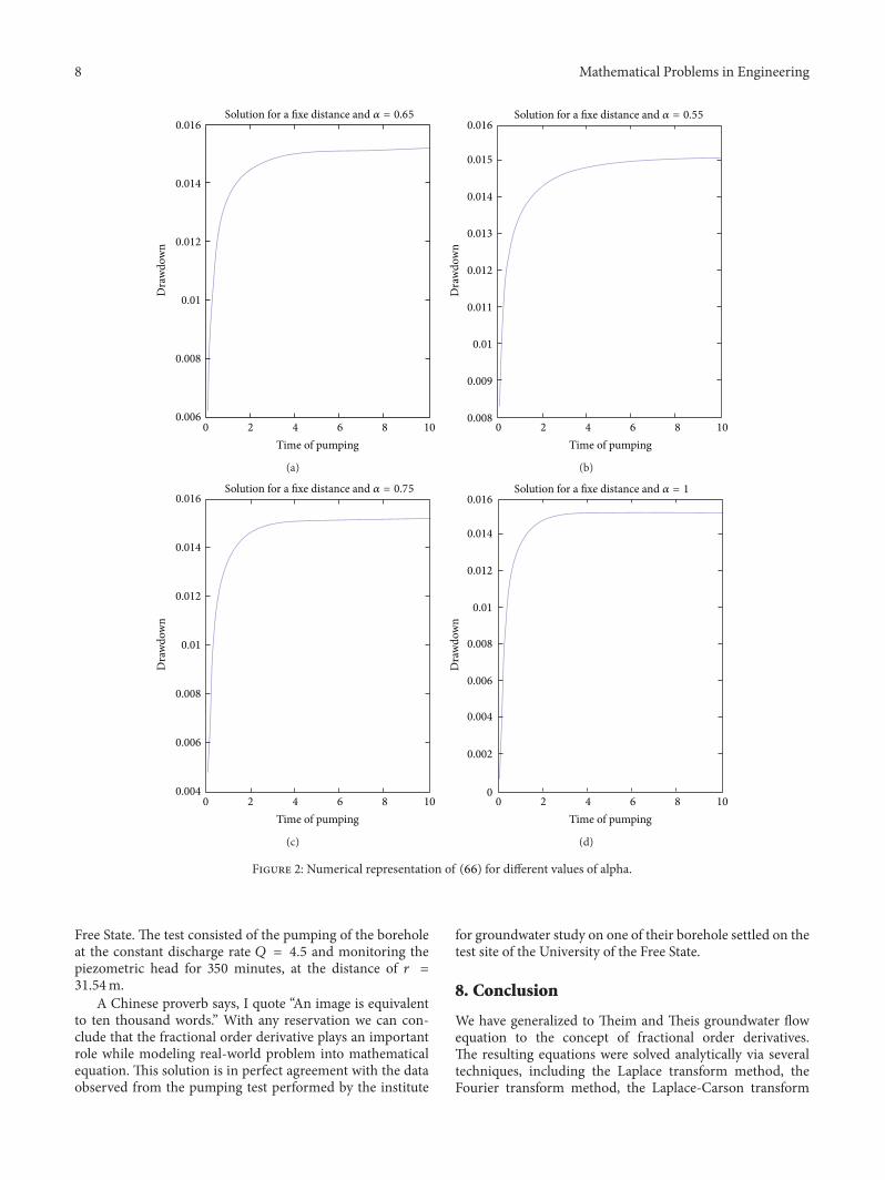
We shall present the numerical solution for the Theis-time-fractional groundwater flow equation for a fixed dis-tance. The analytical solution of the main problem wasdepicted in Figures 2(a), 2(b), 2(c), and 2(d).

We shall present in Figure 3 the comparison of theanalytical solution of theTheis-time-fractional ground waterflow equation, with the experimental data from the pumpingtest performed by the Institute for Groundwater Study on oneof its borehole settled on the test site of the University of the


0.016

0.014

0.012

0.008

0.01

0.006

Solution for a fixe distance and 𝛼 = 0.65

Time of pumping0 2 4 6 8 10

Dra

wdo

wn

(a)


0.016

0.015

0.014

0.013

0.011

0.012

0.01

0.009

0.008


Dra

wdo

wn

(b)

0.016

0.014

0.012

0.008

0.01

0.004

0.006



Dra

wdo

wn

(c)

Solution for a fixe distance and 𝛼 = 1

0.016

0.014

0.012

0.01

0

0.002

0.008

0.006

0.004


Dra

wdo

wn

(d)

Figure 2: Numerical representation of (66) for different values of alpha.

Free State. The test consisted of the pumping of the boreholeat the constant discharge rate 𝑄 = 4.5 and monitoring thepiezometric head for 350 minutes, at the distance of 𝑟 =

31.54m.A Chinese proverb says, I quote “An image is equivalent

to ten thousand words.” With any reservation we can con-clude that the fractional order derivative plays an importantrole while modeling real-world problem into mathematicalequation. This solution is in perfect agreement with the dataobserved from the pumping test performed by the institute

for groundwater study on one of their borehole settled on thetest site of the University of the Free State.

8. Conclusion

We have generalized to Theim and Theis groundwater flowequation to the concept of fractional order derivatives.The resulting equations were solved analytically via severaltechniques, including the Laplace transform method, theFourier transform method, the Laplace-Carson transform


0 50 100 150 200 250 300 350Time

0.5

1.0

1.5

2.0

2.5

3.0

Dra

wdo

wn

Sol. 𝛼 = 0.9270

Obs. data

Sol. 𝛼 = 1

Figure 3: Comparison of Theis-time-fractional groundwater flowequation with experimental data from real observation.

method, and the Boltzmann variable method.The numericalsimulations show that the fractional order derivative playsan important role in the simulation process. In addition, wecompare the analytical solution with experimental data toaccess the accuracy of the fractional groundwater model.Theanalytical solution was in perfect agreement with experimen-tal data.

References

[1] J. F. Botha and A. H. Cloot, “A generalised groundwater flowequation using the concept of non-integer order derivatives,”Water SA, vol. 32, no. 1, pp. 1–7, 2006.

[2] A. Atangana, “Numerical solution of space-time fractionalorder derivative of groundwater flow equation,” in Proceedingsof the International Conference of Algebra and Applied Analysis,p. 20, Istanbul, Turkey, June 2012.

[3] A. Atangana and J. F. Botha, “Generalized groundwater flowequation using the concept of variable order derivative,” Bound-ary Value Problems, vol. 2013, article 53, 2013.

[4] J. Boonstra and R. A. L. Kselik, SATEM 2002: Software forAquifer Test Evaluation, International Institute for Land Recla-mation and Improvement,Wageningen,TheNetherlands, 2002.

[5] G. P. Kruseman and N. A. de Ridder, Analysis and Evaluationof Pumping Test Data, International Institute for Land Recla-mation and Improvement, Wageningen, The Netherlands, 2ndedition, 1990.

[6] H. Jafari and C. M. Khalique, “Homotopy perturbation andvariational iteration methods for solving fuzzy differentialequations,” Communications in Fractional Calculus, vol. 3, no.1, pp. 38–48, 2012.

[7] S. Duan, R. Rach, D. Buleanu, and A. M. Wazwaz, “A reviewof the Adomian decomposition method and its applications tofractional differential equations,”Communications in FractionalCalculus, vol. 3, no. 2, pp. 73–99, 2012.

[8] A. Atangana and E. Alabaraoye, “Solving system of fractionalpartial differential equations arisen in the model of HIVinfection of CD4+ cells and attractor one-dimensional Keller-Segel equation,” Advances in Difference Equations, vol. 2013,article 94, 2013.

[9] D. Baleanu, K. Diethelm, E. Scalas, and J. J. Trujillo, FractionalCalculus Models and Numerical Methods, Series on Complexity,Nonlinearity and Chaos, World Scientific, Singapore, 2012.

[10] A. Atangana and A. Secer, “A note on fractional order deriva-tives and table of fractional derivatives of some special func-tions,” Abstract and Applied Analysis, vol. 2013, Article ID279681, 8 pages, 2013.

[11] G. C. Wu, “New trends in the variational iteration method,”Communications in Fractional Calculus, vol. 2, pp. 59–75, 2011.

[12] G. Jumarie, “On the representation of fractional Brownianmotion as an integral with respect to (dt)a,” Applied Mathemat-ics Letters, vol. 18, no. 7, pp. 739–748, 2005.

[13] G. Jumarie, “Modified Riemann-Liouville derivative and frac-tional Taylor series of nondifferentiable functions furtherresults,” Computers and Mathematics with Applications, vol. 51,no. 9-10, pp. 1367–1376, 2006.

[14] G. Jumarie, “Table of some basic fractional calculus formulaederived from amodified Riemann-Liouville derivative for non-differentiable functions,” Applied Mathematics Letters, vol. 22,no. 3, pp. 378–385, 2009.

[15] A. Atangana, “New class of boundary value problems,” Informa-tion Sciences Letters, vol. 1, no. 2, pp. 67–76, 2012.

[16] S. G. Samko, A. A. Kilbas, and O. I. Marichev, FractionalIntegrals and Derivatives, Translated from the 1987 RussianOriginal, Gordon and Breach, Yverdon, Switzerland, 1993.

[17] C. V. Theis, “The relation between the lowering of the piezo-metric surface and the rate and duration of discharge ofa well using ground-water storage,” Transactions, AmericanGeophysical Union, vol. 16, no. 2, pp. 519–524, 1935.

[18] P. Flajolet, X. Gourdon, and P. Dumas, “Meilin transforms andasymptotics: harmonic sums,” Theoretical Computer Science,vol. 144, no. 1-2, pp. 3–58, 1995.

[19] G. K. Watugala, “Sumudu transform: a new integral trans-form to solve differential equations and control engineeringproblems,” International Journal of Mathematical Education inScience and Technology, vol. 24, pp. 35–43, 1993.

[20] A. Atangana and A. Kılıcman, “The use of Sumudu transformfor solving certain nonlinear fractional heat-like equations,”Abstract and Applied Analysis, vol. 2013, Article ID 737481, 12pages, 2013.

[21] M. G. M. Hussain and F. B. M. Belgacem, “Transient solutionsofMaxwell’s equations based on sumudu transform,” Progress inElectromagnetics Research, vol. 74, pp. 273–289, 2007.

[22] S. Weerakoon, “The “Sumudu transform” and the Laplacetransform—reply,” International Journal of Mathematical Edu-cation in Science and Technology, vol. 28, no. 1, pp. 159–160, 1997.

[23] F. Oberhettinger and L. Badii, Tables of Laplace Transforms,Springer, Berlin, Germany, 1973.

[24] I. Podlubny, Fractional Differential Equations, Academic Press,New York, NY, USA, 1999.

Submit your manuscripts athttp://www.hindawi.com

Hindawi Publishing Corporationhttp://www.hindawi.com Volume 2014

MathematicsJournal of


Mathematical Problems in Engineering

Hindawi Publishing Corporationhttp://www.hindawi.com

Differential EquationsInternational Journal of

Volume 2014

Applied MathematicsJournal of


Probability and StatisticsHindawi Publishing Corporationhttp://www.hindawi.com Volume 2014

Journal of


Mathematical PhysicsAdvances in

Complex AnalysisJournal of


OptimizationJournal of


CombinatoricsHindawi Publishing Corporationhttp://www.hindawi.com Volume 2014

International Journal of


Operations ResearchAdvances in

Journal of


Function Spaces

Abstract and Applied AnalysisHindawi Publishing Corporationhttp://www.hindawi.com Volume 2014

International Journal of Mathematics and Mathematical Sciences


The Scientific World JournalHindawi Publishing Corporation http://www.hindawi.com Volume 2014


Algebra

Discrete Dynamics in Nature and Society



Decision SciencesAdvances in

Discrete MathematicsJournal of

Hindawi Publishing Corporationhttp://www.hindawi.com

Volume 2014 Hindawi Publishing Corporationhttp://www.hindawi.com Volume 2014

Stochastic AnalysisInternational Journal of

research article the use of fractional order derivative to

Documents