research article modification of pd–h and pd–d thin films
TRANSCRIPT

J. Condensed Matter Nucl. Sci. 5 (2011) 1–6
Research Article
Modification of Pd–H2 and Pd–D2 Thin Films Processedby He–Ne Laser
V. Nassisi∗, G. Caretto and A. LorussoLaboratory of Applied Electronics, Department of Physics, I.N.F.N.,University of Lecce, Lecce-I, Italy
D. Manno, L. Famà, G. Buccolieri and A. BuccolieriDepartment of Material Science, University of Lecce, Lecce-I, Italy
U. MastromatteoSTMicroelectronics, via Tolomeo, 1 200010 Cornaredo, Milano-I, Italy
Abstract
In this work, we performed experiments of absorption of hydrogen and deuterium gas by Pd thin films, and we compared the behaviorof these samples to unprocessed films. We also employed a continuous wave He–Ne laser to irradiate the samples inside the chamberduring the treatment, in order to increase the gas absorption. Using a scanning electron microscope (SEM) and an electron probemicro-analyzer (EDX), we observed structures like spots on the surface of the treated samples. Inside the spots, elements other thanPd were found. Based on these results, we determined that gas loading is an effective way to transmute elements, and the laser actionhas been a very effective way to increase morphological changes in the treated samples.© 2011 ISCMNS. All rights reserved.
Keywords: Cold fusion, Laser, Palladium thin film, Silicon, Transmutation
1. Introduction
In March 1989, Fleischmann and Pons [1] reported a large amount of excess enthalpy, and a weak level of radioactivity,from electrolytic cells with Pd cathodes during the electrolysis of D2O. The effect only occurred when a critical thresholdof the stoichiometric ratio x = [D]/[Pd] of deuterium in palladium is achieved. The main point at issue was that theclaimed excesses of enthalpy were consistent only with a nuclear process (deuterium fusion) and that such a process atambient temperature and without the emission of a commensurate number of neutrons was considered to be inconsistentwith modern nuclear science.
∗E-mail: [email protected], Tel.: +39-832-297495, Fax.: +39-832-297482
© 2011 ISCMNS. All rights reserved.

2 Mastromatteo et al. / Journal of Condensed Matter Nuclear Science 5 (2011) 1–6
Figure 1. Boron ion distribution vs. target depth.
In the years following the announcement, many replications of excess heat and helium have been published [2,3],and many new methods to improve the stoichiometric ratio x have been studied [4]. Possible theoretical explanationsof the reported phenomena were proposed [5,6] but they are still far from explaining all results.
Recently the gas loading method became a very effective tool to obtain high absorption of D or H gases inside Pdmetallic lattice, while at the same time keeping the level of contamination low [7]. Important results were achieved bythis method and particular attention has been paid to reproducing transmutation effects [8].
In this work, our attention was devoted to the transmutation phenomenon utilizing Pd film samples treated by gasloading. We also implanted B in these samples in order control the nuclear processes the way Iwamura et al. have done.The treatment of the samples was combined with a continuous wave He–Ne laser light to enhance gas loading insidePd thin films, as in previous studies [9].
2. Experimental Set-up and Results
Using the thermal evaporation technique, we fabricated Pd thin films of 500 nm thickness deposited on Si wafers ofabout 1 cm2 surface area. A 50 nm Ti layer was used to improve the adhesion between the substrate and the Pd layer.
Figure 2. Photo of experimental set-up showing the irradiated chamber.

Mastromatteo et al. / Journal of Condensed Matter Nuclear Science 5 (2011) 1–6 3
Figure 3. Schematic drawing of the experimental set-up. D2: Deuterium gas at 4 bar pressure; T: Target; W: Quartz window; L:Convergent lens;Laser: CW He–Ne λ = 648 nm and Power density = 2 mW/cm2.
These samples were implanted with B ions; a 150 keV accelerating voltage produced a maximum ion concentration at158 nm depth in the palladium layer. Figure 1 shows the distribution of B ions versus target depth.
The thin film samples were placed in cylindrical stainless steel chambers of about 250 cm3 in volume. Figure 2shows a photo of the experimental set-up.
The chambers were equipped with at least one quartz window to allow the laser beam to irradiate the samples. Toavoid contamination, the chambers were carefully cleaned with acetone and dried in nitrogen flux before the experiment.Subsequently a pair of Pd/Si samples has been placed inside the chambers filled with H2 or D2 gas to a maximum pressureof 4 bar. In Fig. 3, we have a schematic drawing of a chamber.
Figure 4. Spots on the surface of a sample with 76 days of treatment (by D2 gas only).

4 Mastromatteo et al. / Journal of Condensed Matter Nuclear Science 5 (2011) 1–6
Figure 5. EDX spectrum of a sample with 76 days of treatment (by D2 gas only). We can observe the presence of the following elements: C, O,Ca, Al, S, Mg, K, Na.
The samples were gas loaded, and one sample for each chamber was irradiated by a CW He–Ne laser(λ = 648 nm) from 16 July to 29 September 2004, at a laser power density of about 2 mW/cm2.
After the treatment ending, the samples were analyzed by a Scanning Electron Microscope (SEM) andan EDX micro-analyzer. Different behaviors were revealed for samples kept in air, laser treated and with-out laser treatment. With the samples kept in air, the film surface was smooth, with a mirror-finish. The
Figure 6. Spots on the surface of a sample with 76 days of treatment (by H2 gas and by He–Ne laser action).

Mastromatteo et al. / Journal of Condensed Matter Nuclear Science 5 (2011) 1–6 5
Figure 7. EDX spectrum of a sample with 76 days of treatment (by H2 gas and He–Ne laser). We can observe the presence of the followingelements: C, O, Ca, Fe, Al, S, Mg, K, Na, F, Cr, Mn, Co, Ni.
samples placed in deuterium gas but not treated with lasers showed morphological modifications of the Pd-film due to the gas absorption. Those treated with lasers showed even more morphological modifications.The modifications consisted of the formation of spots with dimension of 1–50 µm after gas loading.Figure 4 shows an example of spots on the surface of a sample of palladium implanted with boron, loaded by D2gas, but not laser irradiated.
Table 1. The principal detected elements in every experiment.
H2 D2Laser No-laser Laser No-laserSi Si Si SiPd Pd Pd Pd
Ti Ti Ti TiC C CO O OCa Ca CaK K KNa Na NaAl Al AlCr Mg MgFe SCONiMnSF

6 Mastromatteo et al. / Journal of Condensed Matter Nuclear Science 5 (2011) 1–6
By EDX analyser, we investigated inside the spots and found the presence of new elements such as C, O, Ca, Fe,Al, S, Mg, K and Na. In Fig. 5, an example of the EDX spectrum of a Pd sample with 76 days of treatment is shown.It is possible to observe the presence of many “new” elements which were not present before the treatment.
In addition, by He–Ne laser action, we found a larger number of spots and a larger number of new elements.Figure 6 shows a SEM micrograph of a sample processed by H2 gas and laser; Fig. 7 shows EDX spectrum obtainedfrom one spots of the sample: the new elements were: C, O, Ca, Fe, Al, S, Mg, K, Na, F, Cr, Mn, Fe, Co, and Ni.
Table 1 shows the new elements reported in the experiments. We observe that the combination between H2 gasloading and laser action on the treatment of the samples is an effective method of producing many transmutationelements. The results with D2 gas loading alone, without laser irradiation, also produce new elements, and there areno evident differences between the number and type of elements produced with and without the laser. The laser actionincreases the spot density on the surface of the treated samples, but it does not change the nature of the reaction. All newelements were found inside the spots. None of them seems to be generated from a particular nuclear reaction betweenB and D2 and H2. These experiments confirm the reproducibility of the transmutation phenomenon but we are still farfrom clarifying the mechanism inside the crystalline lattice of Pd samples that causes the transmutations.
References
[1] M. Fleischmann, S.J. Pons, J. Electroanal. Chem. 261 (1989) 301.[2] A.B. Karabut, ICCF9, Beijing, China, May 19–24, 151 (2002).[3] F. Celani, A. Spallone, P. Tripodi, A. Petrocchi, D.Di Gioacchino, P. Marini, V. Di Stefano, S. Pace, A. Mancini, Phys. Lett. A
214 (1996) 1.[4] A. De Ninno, A. La Barbera, V. Violante, Phys. Rev. B 56 (1997) 2417.[5] M. Fleischmann, S. Pons, G. Preparata, Nuovo Cimento A 105 (1992) 763.[6] A. Takahashi, ICCF9, Beijing, China, May 19–24, 343 (2002).[7] F. Scaramuzzi, Survey of Gas Loading Experiments, in Second Annual Conference on Cold Fusion, The Science of Cold
Fusion, Como, Italy, 1991.[8] Y. Iwamura, T. Itoh, M. Sakano, S. Sakai, S. Kuribayashi, ICCF-10, Cambridge, MA, Aug. 24–29, 68 (2003).[9] V. Nassisi, Fusion Technol. 33 (1998) 468.

J. Condensed Matter Nucl. Sci. 5 (2011) 7–16
Research Article
Study on the Phenomenon Reported “Neutron Generation at RoomTemperature in a Cylinder Packed with Titanium Shavings and
Pressurized Deuterium Gas”
Takayoshi Asami ∗Research Institute of Innovative Technology for the Earth (retired), 9-2 Kizugawadai, Kizu-cho, Soraku-gun, Kyoto 619-0292, Japan
Abstract
This paper describes the analysis and study of the neutron generation experiment performed under pressurized and/or evacuatedconditions between room temperature and liquid nitrogen temperature, using titanium shavings and deuterium gas packed in acylinder. To clarify the mechanism of this phenomenon, the author has studied the experiment taking into account the characteristicsof the phase equilibrium, the metal crystal construction, the theory of chemical bond and the first principle molecular orbitalcalculation. From the result of this study, it seems that the same phenomenon will happen in a similar experiment performed usinganother electron deficient metal with a suitable crystal construction.© 2011 ISCMNS. All rights reserved.
Keywords: Crystal lattice, Deuterium, Neutron generation, Octahedron cage, Tetrahedoron cage, Titanium
1. Introduction
There are many reports on deuterium nuclear fusion at room temperature. However, some of them have not had sufficientplausible evidence to prove them and the others are doubtful.
Out of these reports, the experiments performed by ENEA, etc. appear to have been performed by suitable devicesand measurement methods [1–3]. Although it is preferable that more reproducible experiments will be executed, wecannot deny the experimental results. It seems that they achieved neutron generation using titanium shavings anddeuterium, which is performed in a process similar to that of deuterium adsorption and desorption.
The author has intended to study the behavior of deuterium in each process of the experiment, and has studiedthe conditions for deuterium atoms or deuterons to collide and the possibility of nuclear fusion occurring at roomtemperature, applying both the theory of chemical bond and the first principle molecular orbital calculation.
∗E-mail: [email protected]
© 2011 ISCMNS. All rights reserved.

8 Takayoshi Asami / Journal of Condensed Matter Nuclear Science 5 (2011) 7–16
2. The Main Process, the Conditions of the Experiment and Explanation of Each Step
According to the experiment performed by ENEA [1] and LANL [2], neutrons are generated during the course ofwarming the cylinder containing pressurized deuterium and titanium shavings with adsorbed and/or combined deu-terium, and at the condition of nonequiliblium such as a change of particular temperature and pressure in the processof adsorption/desorption of deuterium in titanium.
The main process of the experiment and the conditions of the experiment are as follows:
Step 1: It is the generation process of the combined material of titanium and deuterium (from here on we will callit “combined material”) by adsorption, etc., under the pressurized condition in the cylinder made of stainless steel.Pressure: 2–5 MPa, Temperature: room temperature
Step 2: It is the process of the cooling of the cylinder (Ca. 80 K) in the liquid nitrogen bath.
Step 3: It is the process of removing the cylinder from the liquid nitrogen bath and leaving the cylinder to warm untilit reaches room temperature (we assume it is Ca. 300 K).
3. Generally Predictable Behavior of Deuterium Inside and/or on the Titanium Shavings in Each Step
In Step 1, deuterium will enter and subsequently diffuse throughout the crystal lattice of titanium metal, forming thecombined material.
According to other experiments dealing with the characteristics of adsorption and desorption, the deuterium behaviorin this process is similar to the graphical curve of pressure-composition isotherm adsorption with the parameter,temperature. In particular, it is similar to the characteristics of substances that also show hysteresis as shown in Fig. 1[4].
The type of titanium crystal has a hexagonal close-packed (hcp) structure. It is said that there are three locations,where deuterium atoms or deuterons are able to be located in titanium crystal. The locations where deuterium atoms areable to locate under the suitable condition are in the tetrahedral interstice (T-site), in the octahedral interstice (O-site)formed by titanium atoms, and in the location between two titanium atoms in the c-axes of the crystal in Fig. 2 [5].
Figure 2 simply shows the structure of titanium crystal lattice and the inferred location of deuterium.In Step 2 (the cooling of the cylinder) the saturated region of deuterium in titanium metal that expresses the length
of the plateau region in the phase diagram indicated in Fig. 1, will become greater than that of room temperature, bythe formation of combined material. In this step, it seems that deuterium atoms will go further into the titanium anddiffuse into the lattice of titanium metal.
In Step 3, because of the temperature rise, in accordance with the characteristics of phase equilibrium, some portionof the deuterium must exit from the constrained state in titanium and the length of the plateau region in the phasediagram becomes less than that at liquid nitrogen temperature. It indicates that some portion of deuterium in thecombined material is released to the gaseous phase over the course of the temperature rise, relating to adsorption phasechange as written standard book.
When we compare the strength of constrained deuterium in T-site and O-site and deuterium in another site, it appearsthat trapping potential depth in the different sites differs with each other because the combined condition with titaniumatoms differs.
According to the experimental results [1,2], it is said that substantial bursts of neutron counts (Ca. 70 and Ca. 100,respectively) were observed after the cylinder was removed from the liquid nitrogen bath. In the one experiment, itsays that the average count in the active period run (at desorption phase from liquid nitrogen temperature warming toroom temperature) was much higher than the previous run (at pressurized condition with thawing terms and coolingcycles). In the other experiment, the pressurized cylinder had to experience several thermal cycles before neutrons were

Takayoshi Asami / Journal of Condensed Matter Nuclear Science 5 (2011) 7–16 9
Figure 1. Pressure-composition isotherm adsorption with the parameter, temperature [4].
detected. About 1 h into the warm up cycle, when the pressurized cylinder was at –30C, high neutron counts (∼85)were observed, followed by smaller bursts.
It is inferred that any reaction must occur in a condition of nonequilibrium, such as a change of pressure and/ortemperature.
4. The State and Behavior of Deuterium Atoms in Titanium Crystal
4.1. Analysis of the state of deuterium atoms in titanium crystal based on the theory of chemical bond
4.1.1. Bonding state of the deuterium atoms and the titanium atoms in the tetrahedron cage
In the following, the author will study the mechanism of the bonding of deuterium atoms with titanium atoms inaccordance with the theory of chemical bond, taking into account the electron orbits of titanium.
The reason why the deuterium atoms are stable in that location must be because they combine with the titaniumatoms by a specified chemical bond. As an example of an electron-deficient substance, when boron forms diborane(B2H6), the boron atoms cause adjacent hydrogen atoms to have ligancy (number of stable positions (potential well)for H(D)) 2 as indicated in Fig. 3 [6,7].
It seems that a deuterium atom and the titanium atoms jointly own the valence electron located outside the argonshell in the electron orbits of the titanium atom; the deuterium atom and titanium atoms form a coordinate bond. In the

10 Takayoshi Asami / Journal of Condensed Matter Nuclear Science 5 (2011) 7–16
Figure 2. The location of deuterons in the titanium crystal lattice [5].
following, we will study why this combination is formed.By the same process as the formation of diborane, it seems that the titanium atoms forming the cage can also cause
the entering deuterium atom to have ligancy 2. The reason why it is deemed so is because the electron orbits and theirrespective number of electrons regarding a titanium and argon atom are as follows:
Titanium: (1s2 2s2 2p6 3s2 3p6) 3d2 4s2
Argon: (1s2 2s2 2p6 3s2 3p6)
According to the theory of chemical bond explained by Pauling [8], there are nine stable orbits, 3d54s4p3, outsidethis shell. Even if these nine orbits are occupied by nine electrons, 0.72 is allocated as metallic orbit, leaving 8.28 foroccupancy by bonding electrons and unshared electron pairs.
On the other hand, the titanium atom has four electrons outside the saturated orbits (argon shell). As comparedto the number of electrons, four, in the part of the titanium electron orbits outside the argon shell and nine, the total
Figure 3. The configuration of atoms in diborane, B2 H6 [6, 7].

Takayoshi Asami / Journal of Condensed Matter Nuclear Science 5 (2011) 7–16 11
Figure 4. Ti cage models with two bridged deuterium atoms.
number of electrons outside the argon shell is far less than the preferred number of electrons to be stable, which is nine.As a result, it seems that the electrons left from the deuterium atoms that entered the titanium metal will move
toward the titanium orbits side. On the other hand, to get to a stable condition, deuterons will have a tendency to jointlyown the electron with the titanium atoms.
As an example of diborane, Ti atom also is electron-deficient substance. So we can easily guess Ti atoms causetwo deuterium atoms to have ligancy 2 as in the case of diborane. So it seems the adsorbed two deuterium atoms willalso form ligancy 2. In this condition, it seems that two Ti atoms will prepare two bridged deuterium atoms indicatedin Fig. 4a. If two orthogonal pairs of two Ti atoms in the T-site will prepare two bridged deuterium atoms per each Tipair, the classical model will be indicated as in Fig. 4b.
This form is equivalent to the Tetrahedral Symmetric Condensate (TSC) model which is presented by Takahashi[9]. It seems that four electrons that have left from each deuterium atom may form bosonized pair [9] in the outerorbit of each Ti atom forming two orthogonal edges of the tetrahedron cage of which the edge is composed of two Tiatoms. According to hypothesis of Takahashi, it says that strong central squeezing force may happen by TSC plus fourspin-regulated (bosonized) electrons. However, the author’s model is a form of combined material produced just afterdeuterium atoms entered into Ti crystal. On the other hand, Takahashi’s model is the form with very short life assumingwhen the reaction happens in transient state under the special condition. So, the author thinks that his model is differentfrom the author’s model, and is a model which is a work in progress.
4.1.2. Geometrical relation of the deuterium atoms in the tetrahedron cage
In the case of titanium, its crystal is in the form of a hcp structure including cages as mentioned above.Assuming that one of the cages is a regular tetrahedron and the titanium atoms are sphere like shape, the diam-
eter of the inscribed sphere, between the three spheres of titanium atoms and within the regular triangular surfaceformed by the centers of three titanium atoms, is approximately 0.502 Å indicated in Fig. 5a. As the diameter of adeuterium atom is approximately 1.06 Å, if the deuterium atom intends to enter the tetrahedron cage, it must not beas a deuterium atom (D) but as a deuteron (d) having lost an electron. In the case of deuterons, it seems that each ofthem will be able to pass through the inlet of the cage provided that Coulomb repulsion is shielded, as its diameter isapproximately 10−4 Å.

12 Takayoshi Asami / Journal of Condensed Matter Nuclear Science 5 (2011) 7–16
Figure 5. Conceptual figure of the tetrahedron cage in titanium crystal. (a) and (b): the diameter of the inscribed sphere.
4.1.3. Deuterons able to exist in the tetrahedron cage
Inside of the tetrahedron cage, the diameter of the inscribed sphere is approximately 0.709 Å indicated in Fig. 5b. Sothe distance from the center of this inscribed sphere to the center of the titanium atom is approximately 1.81 Å. On theother hand, using the average covalent radius of hydrogen, 0.3 Å [10], the estimated Ti–D distance is approximately1.78 Å, assuming that both Ti–D and Ti–H distances are equal. Regarding the bridged Ti–D(-Ti) distance, it mayslightly be longer than that of a single bond of Ti–D which is similar to the example of the distance of B–H(Ca. 1.19 Å) and bridged B–H(-B) (Ca. 1.33 Å) of diborane [6]. Anyhow, the estimated Ti–D distance coincideswell with the distance from the center of the inscribed sphere to the center of the contacting spheres, Ti atoms.
4.1.4. Plausible behavior and possibility of collision of deuterons in the tetrahedron cage
As it is said, in the case of the tetrahedron cage, the location where a deuterium atom or deuteron is able to locate is inthe cage.
As previously mentioned, we can infer that combined material as indicated in Fig. 4 will be formed. After that, asthere is a stable location in the cage, it seems that the deuterium atom or deuteron in the state may intend to get to thestable location as indicated in Fig. 6 if the condition of nonequilibrium state occurs, such as changing of deuterium
Figure 6. Ti cage models with the bridged deuterium atom in the T-site.

Takayoshi Asami / Journal of Condensed Matter Nuclear Science 5 (2011) 7–16 13
Figure 7. The heavy protons model in the O-site. (a), (b): a pair of counter side (plan), and (c), (d): a pair of diagonal side (plan), (e): a pair ofdiagonal side (perspective).
pressure and/or temperature in the cylinder.If plural deuterium atoms or deuterons will enter the cage, collision may occur in the cage.The constrained two deuterium atoms at the edge of the cage without a strong Coulomb repulsion by the bridging
bond of ligancy 2 are electrically neutral. It may be that under this condition, deuterons do not need an enormousamount of energy to collide.
If we estimate the kinetic energy of a free deuterium atom at 80 and 300 K, the energy of each is 6.9 and 25.9 meV,respectively.
4.1.5. The state of the deuterium atoms combined with the octahedron cage formed by titanium atoms
As in the case of the tetrahedron cage, it is said that there is a location where a deuterium atom or a deuteron is able tolocate in the octahedron cage.
If we take out a quadrilateral pyramid cross section from the octahedron cage that is formed by titanium atoms, andset our eyes to the square part composed of two titanium atoms and a summit atom, both the diameters of the inscribedsphere within the top half pyramid and the inscribed sphere within the square cross section are Ca. 1.27 Å. So if thedeuterium or deuteron is located in these locations of O-site, there is more space than in that of the T-site. As it is said,if the heavy proton is located in the center of the O-site, the location is that of the latter of the case mentioned above.In this cross section of the square area formed by four titanium atoms, two titanium atoms must be selected to get tothe stable condition of deuterium atoms by forming the bridging bond of ligancy 2. Geometrically, there is a total ofsix possible independent Ti pairs of chemical combinations with a bridged deuterium atom in this part. These pairs areselected from the side parts and diagonal line parts in the square which is formed by Ti atoms indicated in Fig. 7.
If we assume the two heavy protons are constrained by two diagonally opposite titanium atom pairs indicated inFig. 7c–e, both heavy protons in the cage will be localized along the centerline of the square, and move near thecenter point of the square. If the collision of caged heavy protons occurs, chances are that it will occur by the heavyprotons constrained by two diagonally opposite titanium atom pairs of the different diagonal. However, the length ofthe diagonal is Ca. 4.18 Å and it is slightly longer than two times the estimated Ti–d distance, 3.56Å.
It seems that it is difficult to more precisely estimate the condition for the deuterium to locate by only the theory ofchemical bond.

14 Takayoshi Asami / Journal of Condensed Matter Nuclear Science 5 (2011) 7–16
Figure 8. The distribution of charge density for (2–203) plane of Ti H3 (7.69 at.% H) cluster [11].
4.1.6. The state of the deuterium atoms on the c-axis of titanium crystal
The c-axis length of titanium crystal is Ca. 4.74 Å and it is said that two deuterium atoms can be located on the c-axisbetween titanium atoms [5]. The nearest titanium atom from the deuterium atom is at the end of this axis. If a deuteriumatom combines with a titanium atom, it will be the titanium atom located at the end of the c-axis. Under this condition,we cannot find special condition for deuterium atoms to collide.
4.2. Analysis based on the first principle molecular orbital calculation
At present, there are not only the analysis based on the theory of chemical bond but on the first principles calculations.By comparison an analysis basing on a different stand point, it seems that we will be able to deduce a more precisestate of deuterium in titanium crystal.
As there is the research of electronic structure of the Ti–H solid solution by a first principle molecular orbitalcalculation, the author cites in Figs. 8 and 9 [11]. Figure 8 shows the distribution of charge density around a hydrogenatom on Ti–H solid solution cluster.
Essentially, both the distance and the bonding force between Ti atom and H atom in the symmetrical location canbe the same as each other. The bond between the second nearest Ti atoms (Ti(b)) from the H atom in the center isstrongly formed with each other. However, there is clear difference in the bond between the first nearest Ti atoms (Ti(a))and Ti(b). In diagonally face side Ti atom pairs surrounding H atom, there is a slight difference in the distribution ofcharge density between vertical and horizontal bonds of Ti and H atom in Fig. 8. It seems that there is a possibility thehorizontal 2 face side Ti atoms pair may cause the hydrogen to have ligancy 2, although, of course, the resonance willoccur between these pairs .
Figure 9 [11] shows the density of states of solid solution. In Fig. 9, density of state of 3d orbital of titaniumdecreases with increasing of hydrogen content and that of 4s orbital of titanium also slightly decreases with increasingof hydrogen content. It means that the electrons of 3d orbital of metallic bond is used for bonding between Ti atomsand the hydrogen atom.
In a regular octahedron cage, each orthogonal plane including the center line and the diagonal line of the squareto (2–203) plane also has two diagonally face side Ti atom pairs. So it means that another Ti pair in the other planes

Takayoshi Asami / Journal of Condensed Matter Nuclear Science 5 (2011) 7–16 15
can cause hydrogen to have ligancy 2 if there is a hydrogen atom between them. On the other hand, there is only onelocation where H is stable is in the octahedron cage.
So, in a condition of nonequilibrium state inside and/or outside Ti metal, such as changing deuterium pressureand/or temperature, if deuterium atoms or deuterons scramble the location of each other, collision may occur near thecenter of octahedron cage.
As another inference of this analysis, in Ti metal composed of dense crystal, it seems that it may be difficult for twodeuterium atoms in ligancy 2 to exist as indicated in Fig. 4. except Ti atom pair at cleavage plane and/or metal surface.
In other chance, the author would like to also analyze the tetrahedron cage, from both the theory of chemical bondand the first principles calculations.
5. Discussion and Conclusion
To clarify the mechanism of neutron generation experiment, the author analyzed the site and state of adsorbed deuteriuminto titanium metal, basing on both the theory of chemical bond and the first principle molecular orbital calculation.
As a result, it seems that the titanium atoms forming the cage cause the deuterium atom to have ligancy 2, especiallyat diagonally 2 face side Ti atoms in octahedron cage, from both the theory of chemical bond and the first principlemolecular orbital calculation.
If two bridged deuterium atoms combine with two Ti atoms as “combined material”, as same as that of diboraneand bosonized electrons are produced in the orthogonal Ti pairs of the tetrahedron cage, its form is equivalent to TSCform presented by Takahashi. However, their images of each concept are different from each other.
On the other hand, taking into account of the result of the first principle molecular orbital calculation, it seems thatthe driving force for deuterium to collide may be scrambling force to get to the stable location by the deuterium atomsbetween different diagonally two face side Ti atom pairs in the octahedron cage. This situation may occur in a conditionof nonequilibrium state, such as the change of temperature and/or pressure.
Figure 9. Density of states from (a) Ti, (b) TiH1 (2.70 at.% H), and (c) TiH2 (5.26 at.% H) cluster [11].

16 Takayoshi Asami / Journal of Condensed Matter Nuclear Science 5 (2011) 7–16
If the above-mentioned concept on the room temperature nuclear fusion is right, the observed phenomenon mayalso occur in an experiment under the condition of nonequilibrium state, such as changing pressure and/or temperatureeven with another element which is electron deficient, has suitable crystal construction and adsorbs the deuterium.
Acknowledgement
The author wishes to express sincere thanks to Dr. Takahashi, emeritus Professor of Osaka University, for the valuablesuggestions and discussions on the manuscript.
References
[1] A. De Ninno, A. Frattolillo, G. Lollobattista, L. Martinis, M. Martone, L. Mori, S. Podda, F. Scaramuzzi, Evidence ofemission of neutrons from a titanium–deuterium system, Europhys. Let. 9 (1) (1989) 221, ENEA, Dipartimento TIB, U.S.Fisica Applicata, Centro Ricerche Energia Frascati, C.P. 65-00044 Frascati, Rome, Italy, 1 May, 1989.
[2] H.O. Menlove, M.M. Fowler, E. Garcia, A. Mayer, M.C. Miller, R.R. Ryan ( Los Alamos National Laboratory ), S.E. Jones( Bringham Young University ), Highlights of papers presented at the workshop on cold fusion phenomena , The Measurementof Neutron Emissions from Ti plus D2 Gas”, Santa Fe, New Mexico, May 23–25, pp. 13, 1989.
[3] A. De Ninno, F. Scaramuzzi, ENEA- Area Energia e Innovazione, Dip. Sviluppo Tecnologie di Punta, Centro Ricerche EnergiaFrascati, CP 65, I-00044 Frascati, Italy, AIP Conference Proceedings, Vol. 228, Anomalous Nucear Effects in Deuterium/SolidSystems, PROVO, UT 1990, Emission of Neutron Bursts from a Titanium–deuterium Gas System in a High-efficiency Low-background Eeperimental Setup, p. 122.
[4] Y. Ohsumi, Hydrogen Adsorption Alloy (Suiso Kyuzo Gokin ), Chapter 2 (Agune Gijutu Senta Corp. Ltd., Tokyo, 2000), p. 33.[5] Y. Hukai, Bull. Japan Inst. Metals 24 (8) (1985) 671.[6] L. Pauling, The nature of the chemical bond and the structure of molecules and crystals, An Introduction to Modern Structural
Chemistry, 3rd edn., Cornell University Press, Ithaca, NY, 1960, p. 368.[7] L. Pauling, The nature of the chemical bond and the structure of molecules and crystals, An Introduction to Modern Structural
Chemistry, 3rd edn., Cornell University Press, Ithaca, NY, 1960, p. 363.[8] L. Pauling, The nature of the chemical bond and the structure of molecules and crystals, An Introduction to Modern Structural
Chemistry, 3rd edn., Cornell University Press, Ithaca, NY, 1960, pp. 398–401.[9] A. Takahashi, N. Yabuuchi, On condensation force of TSC, J. Condensed Matter Nucl. Sci. 1 (2007) 97–105.[10] L. Pauling, The nature of the chemical bond and the structure of molecules and crystals, An Introduction to Modern Structural
Chemistry, 3rd edn., Cornell University Press, Ithaca, NY, 1960, p. 227.[11] D. Setoyama, J. Matsunaga, H. Muta, M. Uno, S. Yamanaka, J. Alloys and Compounds 385 (2004) 156–159.

J. Condensed Matter Nucl. Sci. 5 (2011) 17–33
Research Article
Role of PdO Surface-coating in CMNE D(H)-Gas LoadingExperiments ∗
A.Takahashi†, R. Seto and Y. FujitaTechnova Inc., 1-1-1 Uchisaiwai-cho, Chiyodaku, Tokyo 1000011, Japan
A. Kitamura, Y. Sasaki, Y. Miyoshi and A. TaniikeGraduate School of Maritime Sciences, Kobe University, 5-1-1 Fukaeminami-machi, Higashinada-ku, Kobe 6580022, Japan
Abstract
The PdO-coated layer of Pd-nano-particle may arrange fractal nano-dips on its surface when D(H)-gas is charged and de-oxidationmolecules (D2O or H2O) are released. Fractal nano-dips may make local deep adsorption potentials, through which rapid penetrationof D-atoms (ions) into deeper Pd-local lattice (Bloch potential) O-sites of nano-particle may be induced, to realize full or over-fullD(H) loaded state (x >1.0) of PdDx in a short time of the Phase-I process. Formation of D-clusters, such as 4D/TSC on surfacemay be enhanced at nano-dips. A phenomenological model of quasi-free D-motion under constraint of the Bloch potential within aglobal mesoscopic potential well is proposed for the Phase-II phenomena, where nuclear heating by 4D fusion reactions may rathersteadily take place. Generation of collective mesoscopic potential well (CMPW) will make a Pd nano-particle with PdO working as“mesoscopic catalyst” which realizes very large D(H)-loading ratios and anomalously large chemical heat releases both for H-gasand D-gas loading.© 2011 ISCMNS. All rights reserved.
Keywords: Anomalous heat, Collective mesoscopic potential, D-gas loading, Mesoscopic catalyst, Over-full D/Pd loading, Pdnano-particle, Phenomenological model, Role of PdO, Sub-nano dip
1. Introduction
We of the Kobe Group have reported newer results on anomalous D(H) absorption and excess heat by nano-Pd/Metal-Oxide dispersed samples in the JCF10 meeting 1,2 , 5–6 March 2010, Tokyo, and also in the ACS-2010 NET Sympo-sium7, 21–22 March 2010, San Francisco.
∗Note: This paper is submittal to the 9th International Workshop on Anomalies in Hydrogen/Deuterium Gas Loaded Metals, 17–19 September 2010,Siena, Italy.†E-mail: [email protected]
© 2011 ISCMNS. All rights reserved.

18 A. Takahashi et al. / Journal of Condensed Matter Nuclear Science 5 (2011) 17–33
Figure 1. Experimental procedure of D(H)-gas charging to Pd/ZrO2 powder samples and reduction of PdO.
Two new findings were reported there: (1) Forced oxidation of used Pd/ZrO2 samples showed remarkable recoveryeffects on D(H)-loading ratios and heat release rates in the Phase-I interval of D(H)-charging experiments. (2) Bytime-resolved (time-dependent) measurements of D(H)-loading ratios, we have found the “new second phase” after thePhase-I. At the end of Phase-I, D(H)/Pd ratios became 1.1–1.2 with integrated specific heat-energy 0.83–2.0 eV/atom-Pd. At the end of new second phase (Phase-II) with slower change of D(H)-absorption, additional low level heats wererecorded. The third phase (Phase-III) was redefined for the time-period after D(H)/Pd ratios were saturated in Phase-II.We discuss on what kind of underlying physics is there, by proposing a phenomenological model which may relates tothe TSC theory [3–5], for the emerging condensed matter nuclear effects (CMNE).
Reduction process of PdO in samples under D(H) charging is first discussed briefly in this paper. Secondly andmainly, the role of PdO surface coating of Pd nano-particle is discussed using a phenomenological (speculative) modelon what happens under D(H) charging to induce a mesoscopic catalyst potential and the D-cluster formation and 4D/TSCfusion. We summarize discussions as;
(1) The de-oxidation of PdO may be made mostly during the baking processes between D(H)-loading runs, becauseof high level D(H)-density under degassing process at relatively high (473 K) temperature which may enhanceD2O (H2O) chemical formation.
(2) The PdO-coated layer of Pd-nano-particle may arrange fractal sub-nano-dips (sub-nano-holes; SNH) on its

A. Takahashi et al. / Journal of Condensed Matter Nuclear Science 5 (2011) 17–33 19
surface when D(H)-gas is charged and de-oxidation molecules (D2O or H2O) are released to vacuum.(3) Fractal sub-nano-dips may make local deep adsorption potentials, through which rapid penetration of D-atoms
(ions) into deeper Pd-local lattice (Bloch potential) O-sites of nano-particle may be induced, to realize full orover-full D(H) loaded state (x >1.0) of PdDx in a short time of the Phase-I process.
(4) Formation of D-clusters, such as predicted by the TSC theory [3–5] on surface may be enhanced at sub-nano-dipsalready in the beginning of Phase-I D(H)-loading process and 4D/TSC fusion may take place with considerableprobability.
(5) D-motion in a “mesoscopic deep collective potential” of the nano-PdDx system may be quasi-free to enhancetransient D-cluster (4D/TSC [3–5]) formation probability around tetrahedral sites of local Bloch (periodical-lattice) potential inside a PdD nano-particle. This state can be modeled by the non-linear combination of twooscillations, i.e., one (longer pendulum in approximation) by the deep (about 1.5 eV deep) well-type collectivepotential and the other (shorter pendulum) by the lattice-type periodical three dimensional Bloch potential(about 0.22 eV deep). The shorter pendulum may have “high excited energy” to realize very mobile D-motionunder the constraint of three-dimensional local PdD lattice arrangement, within the mesoscopic global deeppotential well.
(6) Generation of collective mesoscopic potential well (CMPW) will make a Pd nano-particle working as “meso-
Figure 2. Comparison of typical heat evolution data for PP (0.1 µm diam. Pd powder), PB (300 mesh Pd-black powder) and PZ(10 nm-Pd-nano-powder dispersed in ZrO2 flakes).

20 A. Takahashi et al. / Journal of Condensed Matter Nuclear Science 5 (2011) 17–33
scopic catalyst” which realizes very large D(H)-loading ratios and anomalously large chemical heat releasesboth for H-gas and D-gas loading.
2. Formation and Reduction of PdO Surface Layer of Pd-nano-particles
Virgin samples of Pd/ZrO2 (PZ in abbreviation) as provided from the maker (Santoku Co., Kobe, Japan) containedoxygen in the form of PdO/ZrO2 with 100% PdO and ZrO2.
Before the first D(H)-charging runs (by the twin system [1,2,7]), we set up PZ samples in reaction chambers of thetwin system, evacuated the chambers and baked samples at 200C to remove “already absorbed” impurity gases. Sincesamples have been reserved in air for a few months, Pd-particles (PdO) would have absorbed a considerable amount ofhydrogen in air (0.01% of air is H2 gas, 1015 H2 molecules per cc air). During a baking process, significant portion ofPdO would have been de-oxidized by forming D2O (H2O) vapors to be evacuated. PZ samples may be a composite of(PdO)yPdx /ZrO2 with x+ y = 1.0. We have then made the first D(H)-charging runs to observe D(H)/Pd loading ratiosand heat–power evolution in Phases I–III. Before the second D(H)-charging runs for used PZ samples, we have madeevacuation and baking. In this second baking stage, we speculate that almost 100% reduction of PdO would have beendone by “water-formation” reactions between out-going D(H) atoms and oxygen atoms in PZ sample under the elevatedtemperature (200C) which enhanced chemical reaction rates. Such an experimental procedure as above mentioned isflow-charted in Fig. 1.
We refer an essential results of Kitamura et al. PLA 2009 paper [6], for heat–power evolution data under D(H)-gascharging to three kinds of Pd powder samples (PP, PB and PZ), as shown in Fig. 2.
How can we explain the results of anomalously enhanced heat–power evolutions for PZ samples both for D- and
Figure 3. Definition of phases I and II intervals for the D(H)-gas loading experiment [6,7]).

A. Takahashi et al. / Journal of Condensed Matter Nuclear Science 5 (2011) 17–33 21
Figure 4. An atomic scale cross sectional image of PdO-layer coated (30%, y = 0.3) Pd nano-particle (5 nm diameter); here we used relative sizesof ionic radii and D2 molecule, and fractal surface structure is supposed to make a role enhancing deeper adsorption potential for D(H)-gas.
H-charging, and why D-charging gave significantly larger heat–power in Phase-I and only gave positive heat–powerlevel in Phase-II? What is a role of PdO component, since the second D(H)-charging runs with used samples (withoutPdO component) gave very reduced D(H)/Pd-loading ratios and heat? Experiments with forced oxidation [1,2] (4–8%of total Pd amounts) to used PZ and PNZ (Pd/Ni/ZrO2) samples showed remarkable recovery for D(H)/Pd ratios (up to1.1–1.8) and heat levels (0.8–2.0 eV) in Phase-I. What is the mechanism for that? Are these phenomena related to theproposed mechanisms of Takahashi’s TSC formation models and D-cluster (4D, typically) fusion reactions?
3. A Phenomenological Model of D(H)-Adsorption/Absorption with PdO Layer
We propose phenomenological models in Sections 3 and 4 for the phase-I and phase-II phenomena as defined in [6].We show a modified figure for helping this purpose in Fig. 3.
From our analysis of forced-oxidization experiments [7], we have speculated that a portion of PdO at the beginningof first (virgin) D(H)-charging run maybe around 30% (y = 0.3 or so). Assuming a formation of PdO surface layer(coating with y = 0.3) of Pd nano-particle, an image of atomic scale cross section of PdO/Pd nano-particle (5 nmdiameter, for instance) is shown in Fig. 4. By TEM image of used sample (as to be reported by Kitamura ICCF 16paper, and also we reported [7,17] at ACSNET 2010), 2–10 nm PdO/Pd particles are dispersed in/on ZrO2 flakes withseveral micro-meter size. We assume here PdO/Pd particles are kept as isolated each other in a supporter ZrO2 flake.Position of oxygen-atom can be interstitial or substitute for Pd-atom, but we draw here simply as substitute of Pd-atom.

22 A. Takahashi et al. / Journal of Condensed Matter Nuclear Science 5 (2011) 17–33
Figure 5. D2O molecule going out. Figure 6. SNH traps D2 incoming.
Figure 7. Eventual double D2 trapping. Figure 8. Eventual 4D/TSC fusion on surface.
We are going to propose a mechanism that oxygen of PdO layer will serve as a “seed” for generating a “sub-nano-hole” (SNH) when D(H)-gas will be started to charge and formation of D2O (H2O) by incoming D2(H2) gas molecule tocombine (de-oxidize PdO) with oxygen. Formed D2O (H2O) molecule will go out to vacuum, and a SNH with chemicalelectron dangling bonds will be generated. As the trapping potential of SNH will be “very” deep (strong sticking forceby electron-dangling bonds), incoming D2 molecules will be doubly (or more) trapped there to form a transient TSC(transitory Bose–Einstein condensate) with certain probability. The image of such TSC formation is speculative at this

A. Takahashi et al. / Journal of Condensed Matter Nuclear Science 5 (2011) 17–33 23
Figure 9. Expanded view of heat–power evolution data by Kitamura et al. [7] for PZ samples.
stage, and we need a further deepened study based on the first principle type quantum-mechanical calculations usingtime-dependent coupled Schroedinger equations for the SNH composition of three dimensional Pd-atoms arrangementand in-coming D2 molecules. However, this is not so easy task.
Once a TSC (t = 0) is formed, very fast (in 1.4 fs) condensation happens to make a very small (in 10–20 fm diam.)charge neutral entity (TSC-min) which will cause 100% 4d-simultaneous fusion to produce two 4He products with heat(23.8 MeV/4He) [3–5]. Image of such a process is illustrated in Figs. 5–8. After such an event of D2 trapping at SNHs,remained surface fractal nano-holes will trap more incoming D(H)-gas and enhance “rapid diffusion” into inner PdDxlattice points (namely O-sites of local PdD lattice), as we speculate existence of “D(H)-pressure” from backside wheretrapping of D2 molecules is taking place one after another and accumulating “surface D-clusters”.

24 A. Takahashi et al. / Journal of Condensed Matter Nuclear Science 5 (2011) 17–33
Figure 10. Normalized heat evolution curves in Phase-I for PZ-1(2)#1 runs [7].
As shown in an inset (right top) of Fig. 7, 1 g of Pd nano-powder contains 5 nm-diam. nano-partilces of 1018 (ofthe order). Since 1011 4d/TSC fusion events corresponds to 1 J, one watt heat-level is maintained by a TSC formationrate of “one over 10 million Pd nano-particles per sec” for PZ sample containing 1 g net Pd atoms. This condition looksfeasible, in reference to observed heat–power evolution levels by Kitamura et al. [1,2,7].
A typical data reported by Kitamura et al. [7] for Phase-I is expanded and is shown in Fig. 9. We can considerthat the heat–power evolution curve for H-charging is purely by chemical heat producing reactions, while the curve forD-charging may have component of some isotope effect, probably “nuclear heating” as shown with specific patterns(see arrows). Data by the twin system [7] gave different end-points of Phase-I for the H-charging and D-charging,respectively, and D(H)/Pd loading ratios are slightly different. We can draw normalized curves by adjusting time-intervals of Phase-I and loading ratios, as shown in Fig. 10.
From Fig. 10, we can have impression that a beginning peak and a later bump of heat-power evolution in theD-charging run look like "nuclear heating components", while bumps around 200 min are due to a pure chemicalheat-power evolution. We have observed and deduced similar normalized heat-power evolution curves, three times,for PZ virgin samples (10 g each) in 2008-2009. Hioki, et al (Toyota Central Research Laboratory) reported8 similarheat-power evolution curve having a very clear peak (sharp spike) in the beginning and a broad bump later for a PZ

A. Takahashi et al. / Journal of Condensed Matter Nuclear Science 5 (2011) 17–33 25
Figure 11. Observed “rapid” heat response is broadened by indicial response of calorimetry, assuming a single exponential “nuclear heat evolutionby D-absorption in Phase-I. Such a “nuclear response” may be a superposed component in observed heat evolution data for D-gas, in comparisonwith rather smooth response by H-gas.
sample (from Santoku Co.) of 54 g. To assure that this is really due to nuclear (fusion) heat, we have of course todetect correlated ash (maybe alpha particles, other minor charged particles, secondary X-rays, EUV and visible lights)on line and/or off-line. This is our future task.
From Fig. 10, we can have impression that a beginning peak and a later bump of heat–power evolution in theD-charging run look like “nuclear heating components”, while bumps around 200 min are due to a pure chemicalheat–power evolution. We have observed and deduced similar normalized heat–power evolution curves, three times,for PZ virgin samples (10 g each) in 2008–2009. Hioki et al. (Toyota Central Research Laboratory) reported [8] similarheat–power evolution curve having a very clear peak (sharp spike) in the beginning and a broad bump later for a PZsample (from Santoku Co.) of 54 g. To assure that this is really due to nuclear (fusion) heat, we have of course todetect correlated ash (maybe alpha particles, other minor charged particles, secondary X-rays, EUV and visible lights)on line and/or off-line. This is our future task.
On the other way of precisely observing time-dependent behaviors of heat evolution in the beginning just afterD(H)-charging, we may obtain anomalously large isotopic effect, namely too large difference of heat–power levels

26 A. Takahashi et al. / Journal of Condensed Matter Nuclear Science 5 (2011) 17–33
Figure 12. Heat evolution curves and η-values for PZ-11(12)#3 runs; nuclear heating looks appearing in the early stage circled by a red brokenelliptic line, for D-gas charging. Amounts of PdO components in PZ-11(12)#3 runs, by forced oxidization, are 8.5 % (5.4 %) for D (H), respectively.
between D-gas and H-gas runs. By exploring such a phenomenon, we may have dynamic information of heat releasemechanisms by “new kind of D-related nuclear reactions” such as 4D/TSC cluster fusion.
We can feel now vividly, by such normalized heat–power evolution runs taken by a twin system, that releasedheat–power by D-charging has a significant component of “some D-related fusion” reactions, due to its time-dependentshapes very different from those for H-charging.
The mechanism of D(H)-absorption in Phase-I is independent of that in Phase-II (the new second phase [2]).The former is a rapid process of absorption with relatively large heat–power level, while the latter looks a slowadsorption/absorption process with relatively weak (about 1/10 of that in Phase-I) heat power level albeit having similarintegrated D(H)/Pd loading ratio components (0.5–1.0). Time-dependent D(H)-absorption rate in Phase-I drew decaycurves of almost same rates both for D- and H-charging. This fact is another background that the heat–power evolutionfor D-charging (Fig. 10) looks like containing component by nuclear origin.
Our calorimetry system had a time resolution (time constant) of 5 min and observed heat evolution curve became aconvolution with its indicial response and exponential absorption rate. If heat release rate is constant (a step function),

A. Takahashi et al. / Journal of Condensed Matter Nuclear Science 5 (2011) 17–33 27
Figure 13. Extended sub-nano dips by D2O formation. Figure 14. Incoming D2 molecules are trapped one after another,by dangling bonds of SNH.
Figure 15. Trapped deuterons diffuse inside with enhanced speedby “D-pressure” from backside.
Figure 16. Feature at the end of Phase-I, full D(H)-loading inO-sites plus surface D-clusters component.
we need to wait about 20 min to get saturated (real) power level. However, if we have rapid heat release, as supposed assome surface nuclear reaction, we may have a local peak of heat–power evolution, as shown by simulation in Fig. 11.
Actually observed example of heat responses by H-charging, namely “pure” chemical heat–power evolution curveand energy per an H sorption (adsorption/absorption), η value (13), is shown in Fig. 12, where data by D-chargingare drastically different. These runs after the forced oxidization realized significant recovery of heat–power levels andD(H)-loading ratios, in reference to the virgin runs. Heat evolution just after the D-charging has a peak, (see arrows)while that by the H-charging slowly rises without a “corresponding peak”, which is considered (speculated) due to thesurface 4D/TSC fusion as shown in Fig. 5. The secondly interesting point is that the D-charging gave more than twicelonger-lasting (about 10 hours) heat power than that (about 3 hours) of the H-charging. Evolutions of time-dependentη values are compared between the D-gas charging and the H-gas charging to show “drastic isotopic effect”. Such abig “isotopic effect” is difficult to be explained by usual chemical (electrons-interaction) effects, and needed to explore

28 A. Takahashi et al. / Journal of Condensed Matter Nuclear Science 5 (2011) 17–33
Figure 17. Surface and inner D(H)-trapping potential for a bulk-character Pd metal [9].
some “nuclear origin”. Ratio of η values (η-D/η-H) are very large (more than 10) in the beginning few minutes afterD(H)-charging. Such a big isotopic effect infers the need of explanation by a rapid heat release mechanism of somenuclear reaction as 4D/TSC fusion on surface.
Now we come back to follow the simulation after Fig. 8 for D(H)-absorption into Pd nano-particle. Double D2trapping in an SNH does not always make a TSC, but does make reaction with near-by oxygen to form D2O moleculesand extended SNH as shown in Fig. 13. Through the extended SNH, deuterons trapped diffuse to inner O-sites asshown in Fig. 14.
In Fig. 15, we draw an image of D-diffusion enhanced by pressure of incoming deuterons from behind through theextended SNH. Finally, at the end of Phase-I, Pd nano-particle is fully loaded (PdD, x = 1.0), but we have additionaltrapped deuterons on surface (in SNHs) and apparent x-value becomes more than unity, typically as we can roughlycalculate from the drawing, x = 1.1–1.5 which agrees well with observed Phase-I D(H)/Pd ratios [1,2,7]. This featureis drawn in Fig. 16.

A. Takahashi et al. / Journal of Condensed Matter Nuclear Science 5 (2011) 17–33 29
4. A Phenomenological Model in Phase-II
As shown in Fig. 16, PdD local lattice may be formed inside a Pd nano-particle in Phase-II. We have in additiontrapped deuterons (possibly making D-clusters) on surface SNH. For a known characteristics of bulk Pd metal for D(H)absorption, we have potential forms as shown in Fig. 17 for the surface adsorption and trapping (absorption) in innerlattice O-sites [9].
The surface adsorption energy (depth of potential) is 0.5 eV and lattice absorption energy is 0.2 eV, as evaluated ina standard text book [9]. Therefore heat release level for a bulk Pd sample is around 0.2 eV per D(H)-absorption, sincenumber of trapped deuterons on surface is negligible. In contrast, observed specific absorption energy by PZ (and PNZ)samples are very large, namely around 2.0 eV per D(H), about 10-fold of the bulk value (0.2 eV). To explain observedanomalous values of D(H) loading under as “rapid loading process as observed” and such high specific “chemical”heat-energy level, we need to propose some new mechanism. We speculate and model that surface adsorption potentialbecomes very deep as 1.5–1.8 eV for a nano-Pd particle and local periodical Bloch potential should be in “shrunkenstate as shown in right figure of Fig. 18. Here anomalously high chemical heat releases are considered both for D-gasand H-gas charging procedures.
Existence of PdO surface “barrier” and formed SNHs would make very deep D(H) adsorption potential on surface(1.5–1.8 eV deep, speculated by our experiments [9]), which is categorized as an collective mesoscopic potential well
Figure 18. Collective shrunken state potential of Pd nano-particle for D(H) trapping, right figure, compared with a bulk metal trapping potential,left figure.

30 A. Takahashi et al. / Journal of Condensed Matter Nuclear Science 5 (2011) 17–33
Figure 19. Quasi-free motion of deuterons inside CMPW potential enhances TSC formation around T-sites of local PdD lattice of Pd nano-particlewhich has formed a collective mesoscopic potential well (CMPW).
(CMPW, or a global potential for a nano-particle). Inside a CMPW confinement, three-dimensional PdD lattice (Bloch)potential exists as local fine structure in “shrunken state”.
The CMPW potential induces a QM non-harmonic oscillation, and the local Bloch potential induces a QM harmonicoscillation (wave function becomes a Hermite function, of which ground state is Gaussian and highly excited state has aU-shape wave-function). Two QM oscillations combine non-linearly [14] to make D-motion in a nano-Pd particle highlyfree (quasi-free) under the three dimensional constraint of PdD Bloch structure. This quasi-free motion of deuteronsinside a mesoscopic nano-particle enhances very much probability of TSC (tetrahedral symmetric condensate [3–5])formation as we give an image of QM wave superposition in Fig. 19 [10].
Generation of CMPW will basically make a Pd nano-particle working as “mesoscopic catalyst” which realizesvery large D(H)-loading ratios and anomalously large chemical heat releases both for H-gas and D-gas loading. Ifanomalously large heat observed for H-gas run is by this process, some endothermic (slow heat sink) process shouldexist before we made de-sorption runs for which we observed [13] only about 1/10 levels of heat absorption, comparedwith released heat levels for the sorption runs, both for D- and H-absorbed samples.

A. Takahashi et al. / Journal of Condensed Matter Nuclear Science 5 (2011) 17–33 31
Figure 20. Speculation of useful potential forms to be applied for QM calculations to estimate fusion reaction rates from a simple system to manybody, mesoscopic and bulk condensed matter systems.
In Fig. 20, we show a flow-chart drawing of considered useful potential forms in Coulombic (electro-magnetic)and nuclear strong interaction, starting from a simple system of atom and two nucleons to more complex systems asD-cluster, mesoscopic nano-particle and bulk material. By defining useful potentials for interactions in every step, wecan extend quantum-mechanical (QM) analysis by using many body Schroedinger equations (or dynamic equations asQM-Langevin equation [3–5]). Fusion reactions in microscopic random systems (gas and plasma) can be treated byusing a simple Coulombic potential and a one pion exchange potential (OPEP) [11]. For D-cluster systems, we canapply special trapping potential-forms for Coulombic interactions based on Platonic symmetry (orthogonal coupling)between electron wave functions and deuteron wave functions. For multi-body strong interactions of 4D, 6D, 8D, etc.cluster fusion reactions, we can use an empirical formula of PEF (pion exchange force) [12].
The specific nature of condensed matter is of constraint (ordering or self-organization) motion of particles withlattice regularity or surface fractals. A global shrunken state potential well for trapping D(H) atoms in deep hole willrealize a non-linear oscillation mode coupled with harmonic oscillation in PdD lattice, which makes deuteron motioninside a nano-particle quasi-free under ordered constraint to induce enhanced cluster (TSC) formation probability. Abulk Bloch potential (periodical) is useful for established states of D(H) absorption. We speculate that D-cluster fusionis induced in the states of D-cluster and D-mesoscopic systems.

32 A. Takahashi et al. / Journal of Condensed Matter Nuclear Science 5 (2011) 17–33
Figure 21. Typical four steps for TSC condensation and simultaneous 4d fusion.
We copy lastly typical four steps of TSC motion and 4d fusion in Fig. 21.
5. Concluding Remarks
(1) With a PdO surface layer, sub-nano-holes (SNH) are formed in the beginning of D(H)-gas charging. This SNHwould become a seed of “anomalous phenomena” in D(H)-loaded Pd nano-particle samples.
(2) PdO layer also helps to make up a global deep mesoscopic trapping potential well which is a shrunken state oflocal PdD lattice Bloch potentials inside a nano-particle.
(3) In SNHs, formation of 4D/TSC is largely enhanced in the Phase-I interval of D(H)-gas loading. 4D fusion thusinduced may be a main nuclear component of heat release in Phase-I.
(4) Within a global mesoscopic potential with local Bloch potentials, quasi-free D-motion is induced by non-linearlycoupled oscillations for the global QM state (long pendulum) and a local harmonic oscillator (short pendulum).Anomalous heat by D-charging in Phase-II may be by 4D/TSC fusion of this process.
(5) Generation of CMPW will basically make a Pd nano-particle working as “mesoscopic catalyst” which realizesvery large D(H)-loading ratios and anomalously large chemical heat releases both for H-gas and D-gas loading.
References
[1] Y. Sasaki, Y. Miyoshi, A. Taniike, A. Kitamura, A. Takahashi, R. Seto, Y. Fujita, Measurements of heat and radiation from Pdnano-powders during absorption of hydrogen isotopes, Proc. JCF10, 2010, to be published.
[2] Y. Miyoshi, Y. Sasaki, A. Taniike, A. Kitamura, A. Takahashi, R. Seto, Y. Fujita, Two absorption/adsorption processes ofhydrogen isotopes observed for Pd nano-powders, Proc. JCF-10, 2010, to be published.

A. Takahashi et al. / Journal of Condensed Matter Nuclear Science 5 (2011) 17–33 33
[3] A. Takahashi, N.Yabuuchi, Study on 4D/TSC condensation motion by non-linear Langevin equation, In ACS Symposium Series998; Low Energy Nuclear Reactions Source Book, J. Marwan, S. Krivit (eds.), American Chemical Society, Oxford UniversityPress, Washington, DC, 2008, pp. 57–83.
[4] A. Takahashi, The basics of deuteron cluster dynamics as shown by a Langevin equation, in LENR Source-Book 2, J. Marwan,S. Krivit (eds.), Washington, DC, American Chemical Society, 2009, pp. 193–217.
[5] A. Takahashi, J. Condensed Matter Nucl. Sci. 2 (2009) 33–44.[6] A. Kitamura, T. Nohmi, Y. Sasaki, A. Taniike, A. Takahashi, R. Seto, Y. Fujita, Phys. Lett. A, 373 (2009) 3109–3112.[7] A. Kitamura, A. Takahashi, Yu Sasaki, Y. Miyoshi, A. Taniike, R. Seto, Y. Fujita, Heat evolution from Pd nanopowders exposed
to high-pressure hydrogen isotopes and associated radiation measurements, J. Marwan (ed.), LENR Sorcebook, vol. 3, AmericanInstitute of Physics, to be published in 2010.
[8] T. Hioki, H. Azuma, T. Nishi, A. Itoh, S. Hibi, J. Gao, T. Motohiro, J. Kasagi, Hydrogen/deuterium absorption capacity of Pdnanomaterials and its relation with heat generated upon loading of hydrogen isotope gases, Proc. JCF10, 2010, to be published.
[9] 9) Y. Fukai, K. Tanaka, H. Uchida, Hydrogen and Metal (in Japanese), ISBN4-7536-5608-x C3042, Material Series, UchidaRokakuho Publ., Tokyo, 2002.
[10] A. Takahashi, T. Iida, F. Maekawa, H. Sugimoto, Y. Yoshida, Fusion Technol. 19 (1991) 380–390.[11] 11) T. Hamada, I. Johnston, Nucl. Phys. 34 (1962) 382.[12] A. Takahashi, N. Yabuuchi, J. Condensed Matter Nucl. Sci. 1 (2007) 106–128.[13] A. Kitamura, A. Takahashi, Y. Sasaki, Y. Miyoshi, A. Taniike, R. Seto, Y. Fujita, Anomalous heat evolution in charging of pd
powders with hydrogen isotopes, J. Marwan (ed.), LENR NET Sourcebook, vol. 3, American Chemical Society, to be publishedin 2010.
[14] B. Ahern, Private communication, 2009.

J. Condensed Matter Nucl. Sci. 5 (2011) 34–41
Research Article
Issues Related to Reproducibility in a CMNS Experiment
Jeff Driscoll254 Shaw Avenue, Abington, MA 02351, USA
Mike Horton26451 Trancas Ct., Sun City, CA 92586, USA
Ludwik Kowalski ∗Montclair State University, Montclair, NJ 07043, USA
Pete LohstreterThe Hockaday School, 11600 Welch Road, Dallas, TX 75229 , USA
Abstract
Unexplained emission of charged nuclear projectiles due to electrolysis has been reported by Richard Oriani. Experimental resultswere said to be highly reproducible. Working independently, we were not able to observe emission of charged nuclear particles (ina chemical process similar to Oriani’s) and therefore are unable to provide supporting evidence that the effect is reproducible.© 2011 ISCMNS. All rights reserved.
Keywords: Cold Fusion, CMNS, LENR, Nuclear Reactions
1. Introduction
Radioactivity, such as emission of alpha particles, has long been thought to be independent of chemical processes,such as electrolysis. The same is true for nuclear reactions including fusion and fission. The reason for this is that thekinetic energies of molecules in a typical chemical process are too small to overcome the Coulomb repulsion betweenpositively charged nuclear particles [1]. This expectation was challenged by Pons and Fleischman [2], Oriani [3, 4], andother scientists, as described by Storms [5]. We were attracted by Oriani’s work because his findings were impressive
∗E-mail: [email protected]
© 2011 ISCMNS. All rights reserved.

Jeff Driscoll, Mike Horton, Ludwik Kowalski and Pete Lohstreter / Journal of Condensed Matter Nuclear Science 5 (2011) 34–41 35
(a nuclear process taking place during electrolysis) and his methodology was simple. Our goal was to either confirmor refute the claimed reproducibility of the effect.
The electrolyte in Oriani’s cell, Li2SO4, is usually dissolved in light water at the concentration of 0.022 g per cubiccentimeter. The cathode electrode is usually nickel while the anode electrode is usually platinum. To detect chargednuclear particles, Oriani uses CR-39 chips. This method of detection is widely used in personal neutron dosimetersas well as in other fields of research [6] such as measuring the amount of radon in the air and studying thermonuclearreactions. In Oriani’s 2003 experiment, described in [3], the detector was suspended in the electrolyte between theanode and the cathode. The mean track density on the experimental chips was 470 tr/cm2 while the mean track densityon control chips was 168 tr/cm2. The corresponding standard deviations were 384 and 99 tr/cm2, respectively.
Referring to such results, Oriani et al. concluded in 2003 that: “a nuclear reaction of as-yet unknown nature canaccompany the electrolysis.” Experimental results, according to Oriani’s more recent 2008 paper [4], are now highlyreproducible. The purpose of the present study was to verify this assertion.
2. Oriani’s Cell and New Experimental Results
The cell used in Oriani’s new study [4] is shown in Fig. 1. It was similar to the cell used in [3]. The essential differencewas the addition of a thin Mylar film (6 µm) placed between the CR-39 detector and the nickel cathode. That filmwas chosen to protect the CR-39 detector from the electrolyte without interfering with detection of expected nuclearparticles.
Twenty-one experiments were performed and 42 CR-39 surfaces were examined, as described in his 2008 paper [6].The track density on one of these surfaces was reported as “too large to count.” Track densities on the remaining 41experimental surfaces ranged from 9 to 498 tr/cm2, as illustrated in Fig. 2. The histogram was drawn without makinga distinction between surfaces facing the cathode and surfaces facing away from the cathode. Note that the distributionof densities is not bell-shaped. Track densities on control CR-39 chips were usually much lower (mean 21 tr/cm2 andstandard deviation 9.7 tr/cm2) than on most experimental chips (mean 122 tr/cm2 and standard deviation 124 tr/cm2).Mean track densities on surfaces facing the cathode, according to data published in [4], were essentially the same asmean track densities on surfaces facing away from the cathode.
On the basis of these observations Oriani concluded that “the present technique has consistently produced evidencethat a nuclear reaction of some sort has been generated in the course of electrolysis.” Investigations described in thispaper were undertaken to determine if Oriani’s results could be reproduced in another laboratory.
3. Our Cells and Experimental Results
Our experiments, done in four separate laboratories, were performed using cells that were similar to Oriani’s cell.Figure 3 displays a generic diagram of our cells. We used the same electrolyte (Li2SO4 in distilled H2O, at the initialconcentration of 0.022 g/cm3) as Oriani; our electrodes were also made from Ni and Pt. Oriani’s nickel cathode wireand our nickel cathode wires were from the same spool. All of us used the 6 µm Mylar which is capable of transmittingalpha particles with energies higher than 2 MeV. Distances between the cathodes and the anodes were approximately3 cm, which is approximately the same as Oriani’s. The essential cell parameters of Oriani’s and our experiments werethe same.
Differences between Oriani’s experiment and our experiment are the following: Platinum wires for the anodes didnot come from the same manufacturer. Oriani’s cathode was spot-welded to a vertical titanium rod, placed inside aglass tube. Vertical parts of our electrodes, on the other hand, were placed into long heat shrink tubes (not shown in Fig.3). Lower parts of our shrink tubes were thermally compressed, to prevent capillary creep of the electrolyte. Also notethat Oriani’s cell exposes the bottom surface (the side away from the electrolyte) of the CR-39 detector to air while our

36 Jeff Driscoll, Mike Horton, Ludwik Kowalski and Pete Lohstreter / Journal of Condensed Matter Nuclear Science 5 (2011) 34–41
Figure 1. A diagram of an Oriani cell from his 2008 paper [4]. Small circles are cross sections of O-rings placed between the two sections of thecell. A clamp (not shown) is used to press the sections toward the CR-39 detector.
cells do not. In our cells, the bottom surface of the CR-39 is in contact with a 25" layer of polyethylene. That layer wasclamped to the cell. The leakage of the electrolyte was prevented by squeezing the CR-39, Mylar and O-ring betweenthe polyethylene and the cell.
Both we and Oriani used Fukuvi CR-39 material purchased from Landauer. The delivered sheets of that materialare protected from scratches and alpha particles in air by a thin layer of polypropylene plastic. That layer usually peelsoff when the sheet is cut into small chips. Our unprotected chips were kept in salty distilled water (NaCl concentrationof about 10 mg/cm3). Furthermore, all control chips were kept in unused electrolyte during electrolysis. Salty waterprevents potential accumulation of electric charges on CR-39 surfaces kept in air. This precaution was taken to reducethe possibility that electric charges on CR-39 surface in air might attract or repel radioactive ions. No chips wereexposed to air for more than one hour. One author (P.L.) compared track densities on two CR-39 chips, one kept in

Jeff Driscoll, Mike Horton, Ludwik Kowalski and Pete Lohstreter / Journal of Condensed Matter Nuclear Science 5 (2011) 34–41 37
Figure 2. Oriani’s distribution of track densities from his 2008 paper [4]. The +5 and 500, near the lower right corner, refer to five surfaces wheretrack densities were between 300 and 500.
distilled salty water and in air, for 15 days. The track density turned out to be 30 tr/cm2 on the chip kept in salty waterand 505 tr/cm2 on the chip kept in air. This can be explained by the big difference between ranges of alpha particlesin air (centimeters) and in water (microns). Oriani did not use salty water; he wrapped the chips in aluminum foil andkept them in air. All of our “control” chips were kept in unused electrolyte during the time that the “experimental”chips were exposed to electrolysis.
Like in [4], we typically exposed the experimental chips to electrolysis for three days. During this time the electriccurrent was changing slowly from 60 to about 90 mA, due to the loss of water. The corresponding voltage across theelectrodes was typically 7– 8 V and was kept constant during the experiment. The cell was dismounted after eachexperiment and the CR-39 chip was removed. It was then etched for 12 h in the stirred water solution of NaOH(concentration 6.5 M, temperature 72˚C). The pits on CR-39 surfaces, identified as tracks of nuclear particles, weresubsequently counted under the microscope. The uncertainty of up to plus or minus 5% (in reported track densities)was common due to difficulties in distinguishing tracks from certain surface defects. Each experimenter was given aCR-39 chip with one corner that was exposed to alpha particles from an 241Am source. This helped the experimenterlearn the difference between pits and defects. Pits due to particles from that source are shown in Fig. 4. They had thesame size as pits found on control and experimental chips.
The mean and standard deviation on eight of P.L.’s experimental surfaces were 87 and 46 tr/cm2. The mean andstandard deviation on his five control surfaces were 59 and 38 tr/cm2. This information, as illustrated in the Appendix,can be used to justify the statement that the reported difference between mean track densities on experimental and

38 Jeff Driscoll, Mike Horton, Ludwik Kowalski and Pete Lohstreter / Journal of Condensed Matter Nuclear Science 5 (2011) 34–41
Figure 3. A generic diagram for our electrolytic cells. Small circles are cross sections of the compressed O-ring.
control surfaces, 87–59 = 28 tr/cm2 was not statistically significant, considering small numbers of examined surfaces.The mean and standard deviation on six of M.H.’s experimental surfaces were185 and 73 tr/cm2. The mean
and standard deviation on his eight control surfaces were 192 and 72 tr/cm2. This information was also used tojustify the statement that the reported difference between mean track densities on experimental and control surfaces,185–192 = –7 tr/cm2 was not statistically significant.
The mean and standard deviation on eight of J.D.’s experimental surfaces were 98 and 17 tr/cm2. The mean andstandard deviation on his six control surfaces were 125 and 29 tr/cm2, respectively. This information was used tojustify the statement that the reported difference between mean track densities on experimental and control surfaces,98–125 = –27 tr/cm2 was not statistically significant.
The mean and standard deviation on nineteen of L.K.’s experimental surfaces (excluding three exceptional surfacesfrom experiments 13, 14 and 15 — see below) were 16 and 8 tr/cm2. The mean and standard deviation on his 16control surfaces were 14 and 5 tr/cm2, respectively. This information was used to justify the statement that the reported

Jeff Driscoll, Mike Horton, Ludwik Kowalski and Pete Lohstreter / Journal of Condensed Matter Nuclear Science 5 (2011) 34–41 39
Figure 4. A CR-39 surface seen under the magnification of 40, after 12 h of etching. Small circles are pits due to alpha particles from an Americiumsource. The upper left corner shows a mechanically damaged area.
difference between mean track densities on experimental and control surfaces, 16–14 = 2 tr/cm2 was not statisticallysignificant. In other words, experimental results from our four sets of experiments are consistent with each other. Butthey are not consistent with the results reported by Oriani.
Let us address the issue of extremely high track densities on three surfaces from experiments 13, 14 and 15. Theestimated track density on the up-facing surface of the CR-39 chip from Experiment No. 13 were around 15,000 tr/cm2.This is two orders of magnitude higher than typical densities reported by Oriani [6]. The other side of the chip hadnothing but the usual background. The area covered by copious tracks, nearly two square centimeters, matched thecircle delimited by the O-ring. Distribution of tracks in that area was more or less uniform, except near the boundaries,where the track density decreased progressively.
Copious tracks from Experiment Nos. 14 and 15 were very different from Experiment No. 13. On these twosurfaces, tracks were concentrated in small areas, near a hole drilled in each CR-39 chip. The holes were drilled tofacilitate etching; each CR-39 chip was suspended in the etching solution by means of a thin copper wire threadedthrough the hole. These copper wires were from a telephone cable of unknown origin. The area covered by copioustracks from Experiment No. 14 was about 10 mm2; the estimated track density was 200,000 tr/cm2. The area coveredby copious tracks from Experiment No. 15 was approximately 3 mm2; the estimated track density was close to12,000 tr/cm2. Track densities outside of the small affected areas were about the same as on control chips.
It is remarkable that in each of the three cases of high track density, the mean density on the other side of the chip wasessentially the same as on the control chips. That is very different from what was reported in [4]. The most likely causeof copious tracks was migrating radioactive contamination. Attempts made to identify it were unsuccessful. Alpha

40 Jeff Driscoll, Mike Horton, Ludwik Kowalski and Pete Lohstreter / Journal of Condensed Matter Nuclear Science 5 (2011) 34–41
radioactive substances such as uranium, thorium and radium are known to be present in our environment. One nano-gram of radium, for example, emits 37 alpha particles per second. Testing of nuclear weapons in the 1960s contributedto contamination of our environment with long-lasting radioactive isotopes, tritium and uranium for example. Notethat track densities on our three exceptional surfaces were much higher than those reported in [4].
Project participants worked independently of each other in four different states. Collective results, shown in Table 1,became available to participants only after their own results were submitted to L.K. He collected results after countingtracks on his own CR-39 surfaces. Note that Experiment No. 12 was performed without using the Mylar film. Lowtrack densities resulting from this experiment seem to indicate that all experiments could have been performed withoutMylar. Oriani used Mylar to protect the CR-39 from potential chemical effects. Most tracks on control chips wereprobably due to natural background, most likely due to radon, radium, etc. Concentrations of such substances areknown to be location dependent. That fact was probably responsible for differences between mean track densities onthe control chips of individual researchers.
4. Conclusion: Facts and Interpretations
The purpose of our four independent investigations was to find evidence for reproducible emission of nuclear particlesdescribed in Oriani’s 2008 paper [4]. No such evidence was found. We examined 40 CR-39 surfaces and found onlythree cases of excessive tracks. No excessive tracks were found on the remaining 37 surfaces.
We do not know why we were not able to observe emission of charged nuclear particles (in a chemical process similarto Oriani’s). There could have been a setup or procedural difference between the experiments. Further experimentationis needed to confirm the existence of nuclear particle emission in light water electrolysis, understand the causes of such
Table 1. Track densities on 34 surfaces of our experimental chips. No Mylar was used in Experiment No. 12.
Exp. No. ID Experimental chip (upper side) tr/cm2 Experimental chip (lower side) tr/cm2 Control chip averages tr/cm2
1 P.L. 20 28
59 (from five surfaces)2 P.L. 125 1483 P.L. 89 944 P.L. 99 915 M.H. 128 118
192 (from eight surfaces)6 M.H. 128 1927 M.H. 278 2678 J.D. 121 113
125 (from six surfaces)9 J.D. 87 8510 L.K. 21 23
14 (from 16 surfaces)
11 L.K. 24 2412 L.K. 18 813 L.K. > 10000 1114 L.K. 10 > 1000015 L.K. > 10000 1716 L.K. 31 2017 L.K. 23 818 L.K. 12 2419 L.K. 10 8cr 20 L.K. 11 3

Jeff Driscoll, Mike Horton, Ludwik Kowalski and Pete Lohstreter / Journal of Condensed Matter Nuclear Science 5 (2011) 34–41 41
emission and determine the conditions required for reproducibility.
Appendix: An Example of Statistical Analysis
The mean and standard deviation on eight of P.L.’s experimental surfaces were 87 and 46 tr/cm2. The mean andstandard deviation on his five control surfaces were 59 and 38 tr/cm2. Is the difference between mean track densitieson experimental and control surfaces, 87–59 = 28 tr/cm2 statistically significant? To answer this question one mustestimate uncertainties associated with actually measured track densities (87 and 59). The uncertainty about 87 is46/2.8 = 16, where 46 is the reported standard deviation while 2.8 is the square root of 8 (the sample size consisted ofeight surfaces). Likewise, the uncertainty about 59 was 38/2.23 = 17 tr/cm2, where 2.23 is the square root of 5 (thesample size consisted of five surfaces).
The difference of 28 tr/cm2 is too small to be significant, considering large uncertainties associated with the reportedmean densities (59 and 38 tr/cm2).
The same approach was used to show that differences between mean values on experimental and control chips of–7, –27, and 2 tr/cm2, as reported by M.H., J.D., and L.K. respectively, were also statistically insignificant.
Acknowledgement
Dr. Richard Oriani helped us to design experimental set-ups; Dr. Helen Roberts helped us to perform statistical analysisof experimental data. Constructive criticism from two anonymous referees was also highly appreciated.
References
[1] K.S. Krane, Introductory Nuclear Physics; Wiley, New York, 1987.[2] M. Fleischmann, S. Pons and M. Hawkins, Electrochemically induced nuclear fusion of deuterium, J. Electroanal. Chem. 261
(1989) 301–308.[3] R. A. Oriani and J.C. Fisher, Detection of energetic charged particles during electrolysis, in Condensed Matter Nuclear Science,
edited by P. Hagelstein and S. Chubb, Tenth International Conference on Cold Fusion Conference Proceedings, Cambridge,MA 2003, pp. 577–584.
[4] R.A. Oriani, Reproducible Evidence for the Generation of a Nuclear Reaction During Electrolysis, Proceedings of the 14thInternational Conference on Condensed Matter Nuclear Science, Washington, DC, 2008 (in press).
[5] E. Storms, The Science of Low Energy Nuclear Reaction, World Scientific, Singapore, 2007[6] F.M.F. Ng et al., Nucl. Instrum. Meth. Phys. Res. B 263 (2007) 266.

J. Condensed Matter Nucl. Sci. 5 (2011) 42–51
Research Article
Time-resolved Measurements of Loading Ratios and Heat Evolutionin D2 (and H2)-Pd·Zr Mixed-oxide Systems
Akira Kitamura∗, Yuki Miyoshi, Hideyuki Sakoh and Akira TaniikeGraduate School of Maritime Sciences, Kobe University, 5-1-1 Fukaeminani-machi, Higashinada-ku, Kobe 658-0022, Japan
Akito Takahashi, Reiko Seto and Yushi FujitaTechnova Inc., Uchisaiwaicho 1-1-1, Chiyodaku, Tokyo 100-0011, Japan
Abstract
Using a twin system for hydrogen absorption, we have studied heat evolution and high-energy particle generation by D2 and H2gas absorption into nano-sized mixed oxide powders of palladium and zirconium. We have found very large energy of hydrogenabsorption by Pd·Zr oxide compounds exceeding 1.0 eV/D (or H) together with a very high D/Pd loading ratio, exceeding 1.0. Thesystem has been improved to enable time-dependent measurements of the gas flow rate and loading ratio simultaneously with theoutput heat. It has been revealed that the first phase is divided into two sub-phases; the 1a-phase, where most of the anomalouslylarge output energy is produced with a very high loading, D/Pd ≈ 1.2, and the 1b-phase, where much smaller power is produced asloading increases further by a ratio of about 0.5 with a difference in pressure between deuterium and hydrogen.© 2011 ISCMNS. All rights reserved.
Keywords: D/Pd loading ratio, Heat output, Pd·Zr oxide compounds, Time-resolved measurements, Two sub-phases
1. Introduction
The present work describes experiments on deuterium gas charging of palladium nano-powders in the form of Pd/ZrO2nano-composite. This work is a replication of Arata and Zhang [1], which was in turn a sophisticated, yet simplified,version of the Arata and Zhang’s previous-generation experiments with double-structured reactors [2]. With the newconfiguration,Arata and Zhang report anomalous heat and helium-4 generation. If confirmed, this would be an extremelyimportant phenomenon, so it is crucial that it be replicated if possible. Although successful replications using systemssimilar to the original double-structured reactor with Pd-black have been reported [3,4], few reports of replications ofheat and helium-4 with the new configuration have been published.
We constructed an experimental system to replicate the phenomenon and to investigate the underlying physics[5,6]. The system is composed of two identical reaction chambers, what we call a “twin system” where the chambers
∗E-mail: [email protected]
© 2011 ISCMNS. All rights reserved.

A. Kitamura et al. / Journal of Condensed Matter Nuclear Science 5 (2011) 42–51 43
are designated A1 and A2. Both chambers are equipped for calorimetry. A third chamber, designated B, is equipped fornuclear diagnostics. We have performed heat measurements as well as charged particle measurements under D2 or H2absorption by a variety of palladium nano-powders [5–16] including: 0.1-µmφ Pd powder (PP); 300-mesh Pd-black(PB); oxide composites of Pd·Zr (PZ); oxide composites of Pd·Ni·Zr (PNZ) and oxide composites of Ni·Zr (NZ). Wehave recently reevaluated the loading ratios D/Pd (or H/Pd) and E1 based on a revised value for the volume of the ofthe reaction chamber, which we now estimate is 120 ml. The revised results are as follows:
(a) The loading ratio D/Pd ≈ 0.44 (H/Pd is also ∼0.44) and the first phase absorption energyE1 ≈ 0.26 eV/atom-D(or 0.20 for H) for the PP samples. These figures are in good agreement with those found in the literature[17–22]. The figures for both deuterium and hydrogen increase as a function of the fineness of the samplesurface, where the PP samples have the roughest surface, followed by PB, and PZ is the finest.
(b) For the virgin PB samples, the loading ratios for both D/Pd and H/Pd = 1.3 ± 0.04 and the output energies inthe first phase, E1 = 0.42 ± 0.07 eV/atom-D (or 0.39 for H). These values are 2–3 times larger than for the PPsample.
(c) The virgin PZ samples have shown outstanding performance with very high loading ratios D/Pd = 1.8 ± 0.3(or 1.7 H/Pd) together with the high absorption energiesE1, or the deuteride (hydride) formation energyQD(H)ranging from 0.92 to 1.4 eV/D (and 0.92–1.2 eV/H) depending on how much fraction of PdOx reductioncontributes to the measured values of D(H)/Pd and E1.
(d) The PB and PZ samples have given substantially smaller D/Pd (and H/Pd) ratios andE1 values in their recycleduse. These are smaller than or nearly equal to those for the PP samples. We inferred that these are due to aclumping-together (aggregation) effect of palladium nano-particles.
(e) The outstanding performances of the PZ sample have been significantly restored by oxidizing a small amount(less than 10%) of the sample. The runs after forced oxidization allowed us to measure the hydridation energy,QD(H) = 1.11 ± 0.04 eV/D (0.93 ± 0.09 eV/H), which is about 2 times larger than the adsorption energy, and5 times larger than the absorption energy of a bulk-Pd-metal.
(f) In the second phase, we observed positive output, E2 ∼ 2.5 kJ/g-Pd for the deuterium runs employing both thevirgin PZ and the used-PZ samples and the PNZ sample. However, this was only slightly above the margin oferror, so it will have to be confirmed in further investigation.
In these experiments, we determined the amount of hydrogen isotopes absorbed/adsorbed by the samples of palladiumfrom the gas flow rate multiplied by the duration of the first phase, with the gas flow rate being calculated from a rateof the pressure increase in the reaction chamber at the beginning of the second phase. This determination is reasonableif absorption ends completely when the second phase begins. Otherwise, D(H)/Pd will be underestimated.
In recent tests we have improved the experimental setup by equipping the sub-tanks with pressure gauges to directlymeasure the flow rate and the loading ratio [16]. Deuterium (or hydrogen) gas is stored in this sub-tank beforehand, andthen absorption runs are initiated after closing the gas supply-valve on the head of the gas cylinder to close the system.With this improvement, we can make accurate time-resolved measurements of absorbed amount of gas as well as theflow rate. This enables a measurement of time-dependent sorption energy for each hydrogen isotope (differential heatof hydrogen uptake), which we describe in the present paper.
2. Experimental Procedure
The D2/H2 absorption system is composed of two identical chambers (A1·A2 twin system): one for a D2 gas foregroundrun, and the other for an H2 gas background run. As shown in Fig. 1, each of the twin systems has an innerreaction chamber containing palladium powder and an outer chamber that is evacuated to provide thermal insulation forcalorimetry. The detailed description of the system is given in refs. [14,16]. The statistical error in the output power is

44 A. Kitamura et al. / Journal of Condensed Matter Nuclear Science 5 (2011) 42–51
Figure 1. Schematic of one of the twin absorption systems.
evaluated based on the standard deviation of the longitudinal data, and is 0.67 mW. This is multiplied by the durationof the first phase to give the statistical error in the time-integrated output energy, e.g., 4.0 kJ for a 100-min run.
The data nomenclature is as follows. The run number is designated G-PN#M(A)(d), where G is the gas species (Dor H); P the type of powder (PP, PB, PZ); N the powder identification number; and M the number of times the powderhas been used. The number M is incremented when a sample is baked and then used in another absorption run. Whenthe sample is reused without baking it, in what might be considered a continuation of the same run, the number Mis not incremented. The letter A, B, or C is appended to the number instead. Thus, D-PZ11#3B indicates a run withdeuterium, a PZ powder, powder identification number 11, which has been baked and run 3 times, and then run againwithout baking (run 3B).
Every absorption run is followed by a desorption run, which is carried out by evacuating the reaction chamber. Thisis an endothermic process. The thermal data has occasionally been processed and presented in the data tables with therun designation lower-case “d.” For the example above, data from a desorption run following the 3B absorption runwould be labeled DPZ11#3Bd.
The powder species used in the present paper are mixed oxides of Pd·Zr (PZ) fabricated by Santoku Corporation,Kobe, Japan.
To analyze the heat evolution, we assume that the chemical reaction that occurs during loading is described in Eq.(1) or Eq.. (2). These describe a combination of an oxygen pickup reaction during the formation of D2O (or H2O)with a reduction energy ofQred (expressed as eV/atom-Pd) and a hydridation reaction during the formation of hydrideatoms PdD(H) and surface adatoms with a reaction energy of QD(H) (eV/atom-D(H)).
PdOx +(x + y
2
)D2 = xD2O + PdDy, (1)
PdOx +(x + y
2
)H2 = xH2O + PdHy. (2)
Here a fraction x of Pd is assumed to have been oxidized and reduced by introduction of D2 (H2), while a fractiony of Pd is deuterized (or hydrized).

A. Kitamura et al. / Journal of Condensed Matter Nuclear Science 5 (2011) 42–51 45
Figure 2. Typical variation of output power, WD and WH, and pressure in the reaction chamber, PD and PH.
The specific output energy, E1 either in units of (kJ/g-Pd) or (eV/atom-Pd) is expressed as
E1 = xQred + yQD(H). (3)
The fraction y and the energy QD(H) may include those of bulk hydride formation and adsorption to the palladiumparticle surface as well as other possible reactions. We take the value of Qred = 1.85 eV/atom-Pd (or 1.68 for H) fromthe literature.
The value of y is calculated from the mass conservation law during the gas introduction through the Super Needle:
PR0VR
NAkTR= PRVR
NAkTR+ PV
NAkT+(x + y
2
), (4)
where (VR, PR) and (V , P) are the (volume, pressure) of the upstream (reservoir) tank and the downstream (reaction)chamber subdivided by the Super Needle, respectively, both including the connecting pipes. The left-hand side ofEq. (4) represents the amount (in mol) of D2 (H2) molecules in the reservoir tank before opening the Super Needle,and λ represents the fraction of liquid D2O (H2O), if any, generated as a result of the reduction. The third termon the right-hand side of Eq. (4) then represents the volume (in mol) of D2 (H2) molecules lost to liquefaction orabsorption/adsorption. In the present experimental conditions it is assumed that the water molecules produced throughthe reaction (1) will remain in the gas phase, i.e., λ = 0.
To see the effect of oxygen, the sample was occasionally oxidized or deoxidized deliberately [14,16]. The value ofx is calculated from the pressure decrease during the oxidization process.
3. Experimental Results and Discussion
3.1. Time integrated parameters in absorption/desorption runs for PZ samples
Typical variations of the output power,WD andWH, after the introduction of D2 and H2 gas are shown in Fig. 2 togetherwith the pressure, PD and PH, in each reaction chamber for the PZ13 and PZ14 samples. As seen in the other runsdescribed above, the pressure remains low during the main heat generation period, which we call the first phase.

46 A. Kitamura et al. / Journal of Condensed Matter Nuclear Science 5 (2011) 42–51
In the absence of an apparent anomaly, the first phase heat is dominated by the chemical reaction of absorption andadsorption. In some cases, we have observed positive output in the second phase. In the runs described here, however,we observed no significant output, even when the reservoir pressure was increased to 1 MPa.
Table 1 and Fig. 3, which show the same results described in [16], summarize the parameters integrated over thefirst phase of the runs using PZ11 through PZ14; the specific output energyE1 in units of both kJ/g-Pd and eV/atom-Pd,which is the time-integrated output power per palladium atom; the loading ratio yD (yH) at the end of the first phase,which is calculated from Eq. (4); and the hydridation energy calculated with Eq. (3). Here it is assumed that the watermolecules produced through the reaction (1) will remain in the gas phase, i.e., λ = 0.
The results are briefly summarized as follows. The virgin PZ samples (No. 1 runs) have very large specific outputenergy, E1 = 2.28 ± 0.42 eV/atom-Pd for D-runs or E1 = 2.28 ± 0.29 eV/atom-Pd for H-runs on average, as well asvery high loading ratios, D/Pd =2.31 ± 0.06 or H/Pd = 2.29 ± 0.03.
The specific energy E1 for these “recycle” runs is more than one order of magnitude smaller than the virgin runs.The loading ratios, D/Pd and H/Pd, also decrease for the recycle runs to average values of 0.60 ± 0.10 and 0.49 ± 0.14(by a factor of about 4), respectively. Accordingly, the hydridation energy QD(H) also decreases for the recycle runsto average values of 0.27 ± 0.02 eV/D (0.30 ± 0.08 eV/H) (by a factor of about 3), respectively. These are consistentwith those for the bulk (PP) samples.
We see essentially the same values for E1, D/Pd (or H/Pd) and QD (or QH) in the No. 2 (deoxidized sample)runs as those in the recycle runs. However, the performance characteristics are largely recovered in the No. 3 runs byoxidizing the sample palladium to a small extent (a few percent). The averaged values are: E1 =1.97 ± 0.1 eV/Pd,D/Pd = 1.72 ± 0.09 and QD =1.11 ± 0.04 eV/D for D-runs, and E1 = 1.37 ± 0.06 eV/Pd, H/Pd = 1.44 ± 0.16 andQH = 0.93 ± 0.09 eV/H for H-runs. A detailed discussion of these results is found in [16].
3.2. Time-resolved parameters; loading ratio and specific absorption energy
Since we were monitoring the time-dependent pressure both in the reaction chamber and the reservoir tank constitutinga closed system, we can calculate time-resolved loading ratio D(H)/Pd, defined as LD(H)(t), which is equal to theparameter yD(H) defined in Eq. (1), when we can assume that the water molecules, if any, have negligible volume, i.e.,λ = 0.
Figure 4 shows LD(H)(t) as a function of pressure PD(H) in the first phase for D(H)-PZ13(14)No. 1, D(H)-PZ13(14)No. 2 and D(H)-PZ13(14)No. 3 runs. This relationship between the pressure and the loading ratio cor-responds roughly to the absorption isotherm, since the temperature change during the run is smaller than a few degreesCelsius. We find a similarity between the traces for the No. 1 run (a) and the No. 3 run (c). In both cases there are twodistinct phases, phase 1a and phase 1b. In phase 1a the choice of isotopes, deuterium or hydrogen, has no effect, whilein phase 1b deuterium produces higher pressure.
The transition from the 1a-phase to the 1b-phase occurs at about 60 min for the No. 3 run, which is readily apparentin Fig. 2. The effect of the isotopes (deuterium or hydrogen) appears to be of the same nature as that in [24]. Thepressure during the 1b-phase for the D-runs is about 10 kPa, while that for the H-runs it is about 5 kPa. Note that theNo. 2 run has only the 1b-phase. The hydrogen uptake in the 1b-phase isLD(H) ≈ 0.5 in all cases. These values of thepressure and the hydrogen uptake are consistent with those extrapolated from the values found in ref. [24] which used10-µm-thick palladium foils. From this we infer that the 1b-phase is characteristic of the bulk palladium absorption,and not of the surface adsorption. On the other hand, the 1a-phase is considered to be characteristic of the samplecontaining PdO, since the samples for the No. 2 runs have no oxygen.
From the above results we can exclude the possibility that the anomalously large D(H)/Pd might be due to conden-sation of D2O (or H2O) atoms into the liquid phase with negligible volume, i.e., an overestimation of D(H)/Pd (= y) dueto a nonzero λ (cf. Eq. (4)). Condensation, if it could occur, would be in the 1b-phase at higher pressure. However, the

A. Kitamura et al. / Journal of Condensed Matter Nuclear Science 5 (2011) 42–51 47
Table 1. Summary of the first phase parameters in absorption/desorption runs for PZ11 through PZ14samples. Contribution of deoxidization (oxygen pick-up and water formation) to the output energy is notsubtracted in calculating QD(H) in the case of the virgin sample runs indicated with asterisks*.
Run No. O/Pd (= x)Specific output energy E1 D/Pd(= y) QD (eV/D) Remarks(kJ/g-Pd) (eV/atom-Pd)
D-PZ11No. 1 Unknown 1.69 ± 0.05 1.86 2.37 0.79* VirginNo. 2 0 0.14± 0.01 0.16 0.56 0.28 DeoxidizedNo. 3 0.086 1.88 ± 0.07 2.08 1.81 1.15 OxidizedNo. 3d 0 –0.13 ± 0.01 –0.14 – –No. 3A 0 0.14 ± 0.01 0.15 0.56 0.27No. 3Ad 0 –0.11 ± 0.01 –0.12 – -No. 3B 0 0.12 ± 0.01 0.14 0.49 0.28No. 3Bd 0 –0.11 ± 0.01 –0.13 – –D-PZ13No. 1 Unknown 2.44 ± 0.13 2.69 2.25 1.20* VirginNo. 1d 0 –0.27 ± 0.03 –0.30 – –No. 1A 0 0.16 ± 0.02 0.18 0.63 0.28No. 1Ad 0 –0.16 ± 0.02 –0.18 – –No. 1B 0 0.15 ± 0.01 0.16 0.70 0.23No. 1Bd 0 –0.14 ± 0.01 –0.16 – –No. 2 0 0.26 ± 0.06 0.23 0.59 0.39 DeoxidizedNo. 2d 0 –0.17 ± 0.02 –0.18 – –No. 3 0.073 1.69 ± 0.17 1.87 1.63 1.06 OxidizedH-PZ12No. 1 Unknown 1.80 ± 0.13 1.99 2.26 0.88* VirginNo. 2 0 0.14 ± 0.01 0.16 0.45 0.35 DeoxidizedNo. 3 0.054 1.18 ± 0.05 1.31 1.28 1.02 OxidizedNo. 3d 0 –0.10 ± 0.01 –0.11 – –No. 3A 0 0.11 ± 0.01 0.12 0.41 0.29No. 3Ad 0 –0.10 ± 0.01 –0.11 – –No. 3B 0 0.10 ± 0.01 0.11 0.44 0.25No. 3Bd 0 –0.09 ± 0.01 –0.10 – –H-PZ14No. 1 Unknown 2.32 ± 0.12 2.56 2.31 1.11* VirginNo. 1d 0 –0.42 ± 0.05 –0.46 – –No. 1A 0 0.13 ± 0.01 0.15 0.35 0.42No. 1Ad 0 –0.16 ± 0.02 –0.18 – –No. 1B 0 0.16 ± 0.02 0.18 0.73 0.25No. 1Bd 0 –0.16 ± 0.02 –0.18 – –No. 2 0 0.19 ± 0.04 0.21 0.65 0.33 DeoxidizedNo. 2d 0 –0.14 ± 0.01 –0.22 – –No. 3 0.061 1.29 ± 0.13 1.43 1.59 0.83 Oxidized
1b-phase is observed also in the No. 2 runs with no oxygen involved. Therefore, it is unlikely we have overestimatedD(H)/Pd because of condensation.
We can define time-resolved specific sorption energy, or differential heat of hydrogen uptake, ηD(H)(t), as the outputenergy per hydrogen isotope atom absorbed/adsorbed, which is calculated as the output energy during a time interval

48 A. Kitamura et al. / Journal of Condensed Matter Nuclear Science 5 (2011) 42–51
Figure 3. First phase parameters in comparison with D-runs and H-runs; specific output energy E1, loading ratio D(H)/Pd, and hydridation energyQD(H).
τ divided by the increment of L(t) in the same interval;
η(t) ≡∫ t+τt
Ws(t)dt
L(t + τ)− L(t), (5)
where Ws(t) is in unit of power per palladium atom including the contribution from the oxygen pickup reaction. Theinterval τ is arbitrary, and chosen here to be the time constant of the calorimetry system. For the samples with nooxygen involved, the hydridation energy QD(H) introduced above is equal to time-averaged value of ηD(H)(t) with τbeing the first phase duration and t = 0. Since both Ws(t) and L(t) are values per palladium (absorber) atom, ηD(H)(t)
is independent of sample constituent, namely whether we use PZ or PNZ or other mixed samples.

A. Kitamura et al. / Journal of Condensed Matter Nuclear Science 5 (2011) 42–51 49
Figure 4. Time-resolved loading ratio, LD and LH, expressed as a function of pressure in PZ13(14)No. 1–3 runs. The first phase appears to bedivided into 1a-phase and 1b-phase.
Figure 5 shows examples of time-resolved sorption energy ηD(H) and loading ratio LD(H) compared with the outputpower WD(H) in the run D(H)–PZ13(14)No. 3. We notice here again that the evolution of heat has two phases dividedat t = 60 min. The heat evolution associated with hydrogen isotope absorption/adsorption proceeds mainly in thelow-pressure 1a-phase below ∼4 kPa. In a difference from LD(H)(t), a not-inconsiderable difference in the effect ofthe isotopes (deuterium or hydrogen) is observed for the heat evolution in the 1a-phase: ηD ≈ 1.33 eV/D, while ηH ≈1.15 eV/H. On the other hand, a relatively small amount of heat is generated in the 1b-phase from 60 to 100 min; ηD ≈0.47 eV/D and ηH ≈ 0.41 eV/H with a moderate isotope effect compared with that in the pressure mentioned above.
It has been found that most of the heat evolution from the samples in the 1a-phase only occurs when oxygen atomsare involved, and the 1b-phase with no oxygen produces much less heat. From this we might infer that the main heatsource is the oxygen pickup reaction. However, it must be emphasized that QD(H) obtained after the contribution ofthe deoxidization subtracted from E1 is still anomalously large, being 1.11 ± 0.04 eV/D (or 0.93 ± 0.09 eV/H), aswas shown in Table 1 and Fig. 3. Therefore, the main heat source in the 1a-phase is related to the presence of oxygen,but it is independent of the deoxidization reaction. From the fact that the 1a-phase proceeds at low pressure with littledifference in the effect of the isotopes (deuterium or hydrogen) on pressure, we conclude that the heat source is on ornear the surface of palladium nanoparticles, or that the reaction is triggered on or near the surface.
What is important is that the hydridation energy QD(H) = 1.11 ± 0.04 (0.93 ± 0.09) eV/D(H) is much larger thanthe bulk hydride formation energy (∼= 0.2 eV) and the surface adsorption energy (∼= 0.5 eV). Huang et al. [23] havereported that differential heat of hydrogen uptake for hydrogen chemisorption reaches or even exceeds 1 eV/H for a

50 A. Kitamura et al. / Journal of Condensed Matter Nuclear Science 5 (2011) 42–51
Figure 5. Time-resolved sorption energy ηD(H), loading ratio LD(H) compared with the output power WD(H) in the run D(H)-PZ13(14)No. 3.
dispersed 2-nm-diameter palladium particles. In the present case of our Santoku samples, however, the mean diameterof the palladium nanoparticles is 10 nm, and oxygen incorporation is necessary for the large hydridation energy.
A phenomenological modeling and discussions on the role of the PdO layer of the Pd-nano-particle and possiblemechanisms relating the anomalous heat component found in the present work to a nuclear origin are given in theseparate papers [15, 25]
4. Conclusion
The hydrogen isotope absorption/adsorption system has been improved to enable time-dependent measurements of thegas flow rate and the D (or H) loading ratio simultaneously with the thermal output power. Runs using the samples afterforced deoxidization and forced oxidization, as well as the virgin runs at room temperature, have revealed interestingfacts. The first phase, in which chemical heat is produced, is divided into two subphases, after which the chemical heat iscompleted. In the 1a-phase, the predominant heat evolution is associated with hydrogen isotope absorption/adsorption,and proceeds under relatively low pressure below about 4 kPa with the specific sorption energy being ηD ≈ 1.33 eV/Dand ηH ≈ 1.15 eV/H. In the 1b-phase, a relatively small amount of heat is generated under an isotope-dependentpressure of several to 10 kPa with ηD ≈ 0.47 eV/D and ηH ≈ 0.41 eV/H. It should be noted that samples tested afterforced deoxidization exhibited only the 1b-phase. The 1a-phase only appears with samples incorporating oxygen.
References
[1] Y. Arata, Y. Zhang, The establishment of solid nuclear fusion reactor, J. High Temperature Soc. 34(2) (2008) 85–93.[2] Y. Arata, Y. Zhang, Condensed Matter Nuclear Science, Proc. 12th Int. Conf. on Cold Fusion, A. Takahashi, Y. Iwamura, K.
Ota (eds.), World Scientific, Singapore, 2006, pp. 44–54.[3] V.A. Kirkinskii, A.I. Kumelnikov, Proc. ICCF13, Sochi, Publisher Center MATI, Moscow, ISBN 978-5-93271-428-7, 2007,
pp. 43–46.[4] J.P. Biberian, N. Armanet, ibid. pp. 170–180.[5] T. Nohmi, Y. Sasaki, T. Yamaguchi, A. Taniike, A. Kitamura, A. Takahashi, R. Seto, Y. Fujita, http://www.ler-canr.org; to be
published in Proc. 14th Int. Conf. Condensed Matter Nuclear Science (ICCF14), Washington, DC, 2008.[6] Y. Sasaki, A. Kitamura, T. Nohmi, Y. Miyoshi, A. Taniike, A. Takahashi, R. Seto, Y. Fujita, Proc. 9th Meeting of Japan
CF-Research Society, 2009, pp. 29–34; http://www.lenr-canr.org/acrobat/SasakiYdeuteriumg.pdf.[7] A. Takahashi, A. Kitamura, T. Nohmi, Y. Sasaki, Y. Miyoshi, A. Taniike, R. Seto, Y. Fujita, ibid. pp. 35–41; http://www.lenr-
canr.org/acrobat/TakahashiAdeuteriumg.pdf.
A. Kitamura et al. / Journal of Condensed Matter Nuclear Science 5 (2011) 42–51 51
[8] A. Kitamura, T. Nohmi, Y. Sasaki, A. Taniike, A. Takahashi, R. Seto, Y. Fujita, Phys. Lett. A 373 (2009) 3109–3112.[9] Y. Sasaki, A. Kitamura, Y. Miyoshi, T. Nohmi, A. Taniike, A. Takahashi, R. Seto, Y. Fujita, to be published in
Proc. 15th Int. Conf. Condensed Matter Nuclear Science (ICCF15), Rome, 2009; http://iccf15.frascati.enea.it/ICCF15-PRESENTATIONS/S7_O5_Sasaki.pdf.
[10] A. Takahashi, A. Kitamura, Y. Sasaki, T. Miyoshi, T. Nohmi, A. Taniike, Y. Furuyama, R. Seto, Y. Fujita, ibid.,/S2_O4_Takahashi.pdf.
[11] A. Kitamura, Y. Sasaki, Y. Miyoshi, T. Nohmi, T. Yamaguchi, A. Taniike, Y. Furuyama, A. Takahashi, R. Seto, Y. Fujita, ibid.,/S3_O2_Kitamura.pdf.
[12] A. Kitamura, A. Takahashi, Y. Sasaki, Y. Miyoshi, A. Taniike, R. Seto, Y. Fujita, to be published in J. Condensed Matter Nucl.Sci.
[13] Y. Sasaki, Y. Miyoshi, A. Taniike, A. Kitamura, A. Takahashi, R. Seto, Y. Fujita, Measurements of heat and radiation fromPd nano-powders during absorption of hydrogen isotopes, Proceedings of JCF10 Meeting, Japan CF-Research Society, 2010,paper JCF10-3.
[14] Y. Miyoshi, Y. Sasaki, A. Taniike, A. Kitamura, A. Takahashi, R. Seto, Y. Fujita, Absorption/adsorption processes of hydrogenisotopes observed for Pd nano-powders, ibid., paper JCF10-4.
[15] A. Takahashi, A. Kitamura, Y. Sasaki, Y. Miyoshi, A. Taniike, R. Seto, Y. Fujita, Role of PdO Surface-Coating of Pd Nano-Particle for D(H) Charging and Cluster Fusion, ibid., paper JCF10-5.
[16] A. Kitamura, Y. Miyoshi, H. Sakoh, A. Taniike, A. Takahashi, R. Seto, Y. Fujita, Anomalous heat evolution in charging of Pdnano-powders with hydrogen isotopes, submitted to LENR-NET Source book 3, ACS, J. Marwan (ed.)
[17] G. Alefeld, J. Voelkl (eds.), Hydrogen in Metals II–Topics in Applied Physics, vol. 29, Springer, Berlin, 1978.[18] A Koiwai, A. Itoh, T. Hioki, Japan Patent 2005-21860 (P2005-21860A).[19] C.P. Chang et al., Int. J. Hydrogen Energy 16 (1991) 491.[20] M.M. Antonova, Sboistva Gidriedov Metallov (Properties of Metal-hydrides), Naukova Dumka, Kiev, 1975; translated by
NissoTsushinsha, Wakayama, 1976 [in Japanese].[21] Y. Fukai, K. Tanaka, H. Uchida, Hydrogen and Metals, Uchida Rokakuho, Tokyo, 1998 [in Japanese].[22] P. Chou, M.A. Vannice, J. Catalysis 104 (1987) 1–16.[23] S.-Y. Huang, C.-D. Huang, B.-T. Chang, C.-T. Yeh, J. Phys. Chem. B 110 (2006) 21783–21787.[24] R. Laesser, K.-H. Klatt, Phys. Rev. B 28 (1983) 748–758.[25] A. Takahashi, A. Kitamura, Y. Sasaki, Y. Miyoshi, A. Taniike, R. Seto, Y. Fujita, Phenomenological Model on the Role of PdO
Surface-Coating in CMNE D(H)-Gas Loading Experiments, to be published in J. Condensed Matter Nucl. Sci..

J. Condensed Matter Nucl. Sci. 5 (2011) 52-71
Research Article
Energy Exchange In The Lossy Spin-Boson Model
Peter L. Hagelstein ∗Research Laboratory of Electronics, Massachusetts Institute of Technology, Cambridge, MA 02139, USA
Irfan U. ChaudharyDepartment of Computer Science and Engineering, University of Engineering and Technology. Lahore, Pakistan
Abstract
Excess heat in the Fleischmann–Pons experiment is observed without commensurate energetic particles, which is inconsistent withknown nuclear reactions. Any proposed model must address this at the outset. At present, we recognize are two general approachesto the problem: mechanisms which transfer the reaction energy directly to a condensed matter mode, which requires the fractionationof a large quantum into many small quanta; mechanisms in which the large energy quantum is converted to kinetic energy over a verylarge number of neighboring nuclei. We have focused on the first approach, and we have found a model that seems to accomplish this.Here we introduce the model, which we call the “lossy spin-boson model”. We find that energy exchange in the lossless spin-bosonmodel is hindered due to destructive interference effects. Augmenting the model with loss removes the destructive interference, andwe use perturbation theory on a specific example for illustration. Feshbach projection operators and the Brillouin–Wigner formalismwhich we adopt to describe loss in the model are reviewed in Appendix A.© 2011 ISCMNS. All rights reserved.
Keywords: Coherent energy exchange, Excess heat, Fleischmann–Pons experiment, Lossy spin-boson model, Theory
1. Introduction
Over the past several years, we have been thinking about models relevant to excess heat in the Fleischmann–Ponsexperiment [1,2]. In these experiments, a prodigious amount of energy is observed, and 4He is seen in the gas phasein amounts correlated quantitatively with the energy produced [3–5]; essentially no energetic particles are observedcorrelated with the energy [6]. This latter aspect of the experiments has drawn our attention over the years as being ofparticular importance.
To understand why, we consider briefly the situation in a “normal” nuclear reaction. In a Rutherford picture, theincident nuclei might be taken to be as classical particles, and similarly the product nuclei might also be thought about
∗E-mail: [email protected]
© 2011 ISCMNS. All rights reserved.

P.L. Hagelstein and I.U. Chaudhary / Journal of Condensed Matter Nuclear Science 5 (2011) 52-71 53
classically. Both energy and momentum are conserved in such a picture, so that the basic kinematic relations for thefinal state products can be determined from a knowledge of the reaction energy and initial state momenta and energies.A consequence of this is that the reaction energy in the case of deuteron-deuteron fusion ends up as kinetic energy of theproton and triton, or neutron and 3He nucleus, in the final state. In the quantum mechanical description of the reaction,energy and momentum conservation similarly requires that the reaction energy appears as kinetic energy of the productnuclei.
In the Fleischmann–Pons experiment, there are no energetic particles commensurate with the energy produced. Inlight of the comments above, one might reasonably conclude that no nuclear reactions take place. But if so, then whatis the source of the energy, and where does the 4He come from? In the early days following the initial announcementof 1989, arguments were put forth that the energy was a result of chemical reactions, or experimental error [7]. Thearguments against chemical reactions include the absence of observable commensurate chemical reaction products, andthat the amount of energy is much greater in some cases than a chemical level of energy associated with all the atomsof the cathode and electrolyte. The primary argument against experimental error at this time is that the effect has beenreported in a very large number of experiments [8,9], where different calorimeters and different types of calorimetryhave been used.
So, what can be the resolution? Energy at the nuclear level is seen in many experiments, 4He seems to be presentas a product that is correlated with the energy produced, and yet there are no commensurate energetic particles aswould be required in a Rutherford-type picture of a nuclear reaction. We are by now sure that energy is produced as anexperimental fact; we are pretty sure that 4He is produced as an experimental fact; and we are sure that commensurateenergetic particles are not present as an experimental fact. In essence, some new kind of reaction seems to be takingplace in a way inconsistent with the Rutherford picture of how a nuclear reaction is supposed to work.
If so, then where does the energy go? From experiment, we measure it as thermal energy; but whatever intermediateforms the energy might appear in prior to thermalization so far is hidden.
There is indirect evidence in the Letts two-laser experiment that the energy goes into optical phonon modes (inthis experiment in particular) stimulated at the beat frequency, since excess heat persists after the lasers are turned off[10,11]. The theoretical question as to how such a thing might happen is at present an open one.
In our efforts to understand the effect, we have been interested in the possibility of the fractionation of a large energyquantum into a very large number of smaller energy quanta [12]. The basic idea is that the initial nuclear reaction energywill be measured in units of MeV, while the characteristic energy of an optical phonon mode as an oscillator is measuredin units of meV. This suggests that perhaps the large nuclear quanta is somehow being split up into on the order of 108
smaller energy quanta. If a mechanism exists to accomplish this, then we might be able to understand how excess heatis produced in the Fleischmann–Pons experiment.
Although this approach has seemed perhaps the most plausible one to us, there is no precedent, and the majorityof our colleagues favor various other approaches. Among the schemes that are presently being considered there areaneutronic fusion schemes in which the reaction products are hidden [13]; there is the approach of Kim wherein thereaction energy is somehow partitioned as kinetic energy among a very large number of deuterium atoms [14]; andthere is the general approach of Widom and coworkers [15] where the reaction products are again hidden. There havebeen a great many proposals for reaction mechanisms put forth over the years, some of which are based on aneutronicmechanisms that are otherwise largely conventional. The intuition associated with such proposals is that a reasonablyunreactive energetic product (such as an alpha) would be able to slow down and thermalize inside the cathode so asto be “hidden”. The measurements described in [6] can be interpreted, based on direct calculations of the associatedsecondary yields, as placing an upper limit on the energy of a product alpha to be conservatively less than 20 keV.In essence, energetic alphas produced at the watt level cannot be “hidden” in a PdD cathode. Since 4He appears as aprimary product of the new process, this upper limit on the kinetic energy is a very severe constraint, and rules out themajority of proposed mechanisms involving 4He that have been proposed. We do not think that it is possible to “hide”

54 P.L. Hagelstein and I.U. Chaudhary / Journal of Condensed Matter Nuclear Science 5 (2011) 52-71
commensurate energetic reaction products [6], and we do not understand what kind of direct physical mechanism iscapable of distributing a large reaction energy (for example, 24 MeV) over more than 104 deuterium atoms as proposedby Kim.
In the case of direct coupling of the reaction energy into condensed matter modes, there is no real precedent forsuch an effect. The results outlined here follow from our recent studies of basic models involving two-level systemsand harmonic oscillators that began around 2000. The thinking behind this kind of model was that the two-level systemwould stand in for two nuclear states with an MeV energy difference, and the oscillator would stand in for a vibrationalmode of the lattice. The question of interest was whether there was any way to exchange energy coherently between thetwo systems; our earlier results (from the previous decade) suggested that that it would be extremely difficult to couplea relevant number of quanta directly from two-level systems to the oscillator. Computations of coupled systems weredone under a variety of assumptions: weak coupling, strong coupling, linear interactions and nonlinear interactions. Inthese computations, energy exchange seemed to be restricted to less than 100 oscillator quanta at a time.
The situation changed qualitatively when we recognized that energy exchange in these systems was inhibited bymassive destructive interference, which could be removed in lossy systems. We presented calculations at ICCF9 in2002 which showed the basic effect [16]. We used a quantum flow formulation at that time, and carried out calculationswhich showed that coherence was maintained under conditions where up to 104 oscillator quanta were exchanged. Thisresult seemed to us to be quite significant, since it showed that coherent energy exchange could occur between two-levelsystems and an oscillator with incommensurate quanta. Following the initial presentation at ICCF9, there seems tohave been little outside interest in the result.
Subsequently, we devoted significant effort to better understand the new models. In the absence of loss, the earlymodels that we had explored are equivalent to the spin-boson model which has received considerable attention in theliterature [17–19] (but much less attention in regard to the issue of energy exchange in the multiphoton regime). Wedeveloped a rotation that allowed us to treat coherent multiphoton energy exchange in the spin-boson model in thesame way as one would analyze linear coupling [20,21]. In this approach, we were able to isolate dressed states whichwere nearly degenerate, but “distant” with regard to the linear coupling of the model, and estimate the indirect couplingbetween them analytically.
The lossy problem is much harder, and to date we have not identified an analogous rotation that would allow asimilar treatment of the problem. However, we have over the years applied a number of different techniques whichhave allowed us to characterize the model and establish important limits. In this manuscript, we begin our discussionof the lossy spin-boson model. We start with a brief consideration of the spin-boson model, and then augment thespin-boson model with loss using a Brillouin–Wigner loss operator. Since the projection operators of Feshbach andinfinite-order Brillouin–Wigner theory were used more often in decades past, we provide a brief review in Appendix A.Finally, we demonstrate explicitly that indirect coupling between distant states is hindered by destructive interferencein the spin-boson model using perturbation theory (which provides for the cleanest demonstration of the effect), andthat the indirect coupling is not hindered in the lossy model (by considering the limit where the loss becomes infinitefor states with an energy excess).
In the course of the review process, a great many criticisms were put forth by a reviewer, who wanted them to beaddressed systematically in this paper. The issues of interest cover a lot of topics, and we chose to focus our attention ona subset of the problems so that papers of manageable size might result. Nevertheless, some of our colleagues thoughtthat the associated discussion might be useful, so we have added selections of the reviewer’s criticisms along with someresponses in Appendix B.

P.L. Hagelstein and I.U. Chaudhary / Journal of Condensed Matter Nuclear Science 5 (2011) 52-71 55
2. Spin-boson Model Augmented with Loss
The spin-boson model is a popular model which includes two-level systems and an oscillator with linear coupling. Earlierversions of the model were investigated in association with NMR research about 70 years ago [17], and extended toproblems involving atoms and electromagnetic fields about 35 years ago [18]. From our perspective, this Hamiltonianis interesting because it describes the most basic interaction between two fundamental quantum models (two-levelsystems and a harmonic oscillator), and more particularly, it sheds light on coherent energy exchange between the twosystems when the two-level transition energy is a large multiple of the oscillator energy.
2.1. Spin-boson model
The Hamiltonian for the spin-boson model is [19]
H = E
hSz + hω0a
†a + V (a† + a)2Sxh. (1)
In this model, E is the transition energy of the two-level systems, hω0 is the characteristic energy of the oscillator,and V is a coupling strength.
Our intuition might lead us to anticipate that energy exchange between the two systems should occur when thetransition energy of the two-level systems is matched to the characteristic energy of the oscillator. This is so when thecoupling is weak. If the coupling is stronger, and if there is a near resonance between the two-level transition energyand three oscillator quanta, then once again energy can be exchanged coherently. The reason that this works is thatthe system is able to maintain coherence over the time that several interactions occur, so that a nonlinear response ispossible even though the coupling is linear.
We have explored energy exchange in this model in the multiphoton regime, with much larger numbers of oscillatorquanta exchanged for a single two-level system quantum [20,21]. Unfortunately, coherent energy exchange in themultiphoton regime is a weak effect that requires very precise level matching. Coherent energy exchange at finite ratesin this model is possible under moderately strong coupling for up to about 50 quanta at a time; for the exchange of evenmore quanta, the constraints on the degree of resonance becomes prohibitive, and the energy exchange rates becomevery small [23].
2.2. Lossy spin-boson model
If we augment the spin-boson model with loss, things change qualitatively in regard to energy exchange in the multi-photon limit as we will show later on in this paper. We write such a model as [22–24]
H = E
hSz + hω0a
†a + V (a† + a)2Sxh
− ih(E)
2. (2)
The loss term in this model is an operator that comes about from an infinite-order Brillouin–Wigner model as discussedin Appendix A. As written, this loss term is completely general, but we are thinking of it as being referenced to theoscillator so as to provide strong loss at energies in the vicinity of the two-level system transition energy.
In regard to the Fleischmann–Pons model, the oscillator here stands in for an optical phonon mode, so that hω0 istens of meV. The transition energyE for the two-level system is assumed to be associated with nuclear energy levels,on the order of MeV. The thought regarding the loss term here is that loss channels for the phonon mode open if thesystem has available several MeV of energy through the disintegration of nuclei that make up the phonon mode.

56 P.L. Hagelstein and I.U. Chaudhary / Journal of Condensed Matter Nuclear Science 5 (2011) 52-71
3. Indirect Coupling in Perturbation Theory
We have argued previously that the introduction of loss into the model leads to an enormous enhancement of indirectcoupling between distant states that are nearly degenerate. To understand this better, if we consider a product basisstate of the form
|S,m〉|n〉,then the Hamiltonian leads to coupling between neighboring states of the form
|S,m± 1〉|n± 1〉.If the two-level transition energy E were matched to the characteristic energy hω0 of the oscillator, then this directcoupling would lead to coherent energy exchange on or near resonance. However, in the multiphoton regime of themodel, we require the exchange of more oscillator quanta to bring the system back into energy balance. As a result, theclosest states which are nearly degenerate are the distant states
|S,m− 1〉|n+n〉, |S,m+ 1〉|n−n〉,wheren is the number of oscillator quanta exchanged. There is no direct coupling between |S,m〉|n〉 and these states;when the coupling constant is sufficiently large there can be a weak indirect coupling. It is this weak indirect couplingthat we are interested in here.
3.1. Indirect coupling in perturbation theory with no loss
Indirect coupling is very weak in the lossless spin-boson model because of destructive interference. We can see thismost readily in a perturbation theory calculation. As an example, we consider indirect coupling in the case where 5oscillator quanta are exchanged between the nearly degenerate basis states |S,m〉|n〉 and |S,m+ 1〉|n− 5〉.
We can develop the perturbative result that we are interested in starting from a finite basis expansion of the form
=∑j
cjj
= c1|S,m〉|n〉 + c2|S,m− 1〉|n− 1〉 + c3|S,m+ 1〉|n− 1〉 + c4|S,m− 2〉|n− 2〉+ c5|S,m〉|n− 2〉 + c6|S,m+ 2〉|n− 2〉 + c7|S,m− 1〉|n− 3〉 + c8|S,m+ 1〉|n− 3〉+ c9|S,m+ 3〉|n− 3〉 + c10|S,m〉|n− 4〉 + c11|S,m+ 2〉|n− 4〉 + c12|S,m+ 1〉|n− 5〉. (3)
The numbering here corresponds to the state definitions indicated in Fig. 1.The finite basis equations for the coefficients can be written as
Ec1 = mE + nhω0 + V1,2c2 + V1,3c3,
Ec2 = (m− 1)E + (n− 1)hω0 + V2,1c1 + V2,4c4 + V2,5c5,
...

P.L. Hagelstein and I.U. Chaudhary / Journal of Condensed Matter Nuclear Science 5 (2011) 52-71 57
|m,n⟩
|m-1,n-1⟩
|m+1,n-1⟩
|m-2,n-2⟩
|m,n-2⟩
|m+2,n-2⟩
|m+3,n-3⟩
|m+1,n-3⟩
|m-1,n-3⟩
|m,n-4⟩
|m+2,n-4⟩
|m+1,n-5⟩E
1
2
3
4
5
6
7
8
9
10
11
12
Figure 1. Basis states involved at lowest order in perturbation theory for indirect coupling with the exchange of five oscillator quanta.
Ec12 = (m+ 1)E + (n− 5)hω0 + V12,10c10 + V12,11c11. (4)
To develop these equations, we require the diagonal and off-diagonal matrix elements of the spin-boson Hamiltonian.The nonzero matrix elements are
〈n|〈S,m|H |S,m〉|n〉 = ME + nhω0,
〈n+ 1|〈S,m+ 1|H |S,m〉|n〉 = V√n+ 1
√(S −m)(S +m+ 1),
〈n− 1|〈S,m+ 1|H |S,m〉|n〉 = V√n√(S −m)(S +m+ 1),
〈n+ 1|〈S,m− 1|H |S,m〉|n〉 = V√n+ 1
√(S +m)(S −m+ 1),
〈n− 1|〈S,m− 1|H |S,m〉|n〉 = V√n√(S +m)(S −m+ 1). (5)
Since our focus is on the indirect coupling between |S,m〉|n〉 and |S,m+ 1〉|n− 5〉, we can keep the correspondingcoefficients c1 and c12, and eliminate the others algebraically. This leads to coupled equations of the form
Ec1 = mE + nhω0 +1(E)c1 + V1,12(E)c12,
Ec12 = (m+ 1)E + (n− 5)hω0 +12(E)c12 + V12,1(E)c1. (6)

58 P.L. Hagelstein and I.U. Chaudhary / Journal of Condensed Matter Nuclear Science 5 (2011) 52-71
Here 1(E) and 12(E) are self-energies, and V1,12(E) and V12,1(E) are indirect coupling coefficients. The lowest-order contribution to the indirect coupling coefficient V1,12(E) is obtained by summing over the different paths
V1,12(E) = V1,2V2,4V4,7V7,10V10,12
(E −H2)(E −H4)(E −H7)(E −H10)
+ V1,2V2,5V5,7V7,10V10,12
(E −H2)(E −H5)(E −H7)(E −H10)+ · · · , (7)
where Hj is the diagonal matrix element of basis state j . There are 10 terms altogether in this summation. Assumingresonance H1 = H12, this sum can be evaluated in closed form to yield
V1,12(E) = 625
64
V 5√n(n− 1)(n− 2)(n− 3)(n− 4)
E4
√(S −m)(S +m+ 1). (8)
3.2. Destructive interference
The indirect coupling term in the lossless case is very small due to destructive interference. This can be seen from acomparison of the summed indirect coupling coefficient V1,12(E) with the first term of the series of Eq. (7). We maywrite
V1,2V2,4V4,7V7,10V10,12
(E −H2)(E −H4)(E −H7)(E −H10)= 625
64
V 5√n(n− 1)(n− 2)(n− 3)(n− 4)
E4
√(S −m)(S +m+ 1)
(S +m)(S +m− 1)(S −m+ 1)(S −m+ 2)
36(9)
If the number of two-level systems is large, then S will be large. This term can be larger than the sum by a factor thatcan be on the order of S4/36, which gives an indication of how effective destructive interference is for this case.
3.3. Indirect coupling in the lossy model
In the augmented version of the problem with loss, the destructive interference can be removed if the loss terms aresufficiently large. We can begin to see this in perturbation theory by using a finite basis approximation with the samebasis states as we used above. This time, the first three expansion coefficients satisfy coupled equations of the form
Ec1 = H1c1 + V1,2c2 + V1,3c3,
Ec2 = (H2 − ih2/2)c2 + V2,1c1 + V2,4c4 + V2,5c5,
Ec3 = H3c3 + V3,1c1 + V3,5c5 + V3,6c6. (10)
Intermediate states (such as 2) which have energies less than E have decay modes available in this model, since thesystem can decay to such states if energy is lost through the decay processes modeled by the loss operator. Other states(such as 3) which are in energy deficit as intermediate states do not have analogous decay modes available, and are

P.L. Hagelstein and I.U. Chaudhary / Journal of Condensed Matter Nuclear Science 5 (2011) 52-71 59
|m,n⟩
|m+1,n-1⟩
|m+2,n-2⟩
|m+3,n-3⟩
|m+1,n-3⟩
|m+2,n-4⟩
|m+1,n-5⟩E
1
3
6
8
9
11
12
Figure 2. Basis states involved at lowest order in perturbation theory for indirect coupling with the exchange of five oscillator quanta in the limitof infinite loss.
free of loss in this model. States that are resonant (such as 1 and 12) are assumed to be stable against zero-energydecay processes.
The expression one obtains in such a model for the indirect coupling coefficient is very complicated, and notparticularly enlightening. As we are interested in the issue of destructive interference between different pathways, wecan eliminate the destructive interference completely by considering a model in which the loss terms are much greaterthan other terms that appear in the denominator. In the limit that the associated loss is infinite, then only pathwayswhich include intermediate states in energy deficit contribute (see Fig. 2). In this limit we sum to obtain
V1,12(E) →[V1,12(E)
]
j=0F(S,M) (j → ∞), (11)
where the j = 0 result is given in Eq. (8), and where the factor F(S,M) evaluates to
F(S,M) = (S −m− 1)(S +m+ 2)(7S2 + 7S − 7m2 − 23m− 18)
36. (12)
We see from this calculation that destructive interference greatly reduces the indirect coupling between distant resonantstates in the original Dicke model, leading to a much larger indirect coupling matrix element.
4. Discussion and Conclusions
We are interested in the possibility that a large nuclear quantum of energy can be fractionated and exchanged with acondensed matter mode. To investigate this possibility, we have focused on the simplest basic physics model whichexhibits coherent energy exchange between relevant quantum systems – the spin-boson model augmented with loss.This model is interesting in that it describes coherent energy exchange at usefully large rates under conditions where alarge two-level system energy quantum is divided into a great many small energy quanta. In our most recent studies withmore realistic and more sophisticated models, the indirect coupling appears to be strong enough to allow for coherentenergy transfer at rates relevant to excess heat production in the Fleischmann–Pons experiment. This provides us withmotivation for pursuing this model and its generalizations.
We presented the spin-boson Hamiltonian along with the generalization to the lossy version of the problem. Althoughone can find in the literature versions of the spin-boson model augmented with loss, these generalizations of the model

60 P.L. Hagelstein and I.U. Chaudhary / Journal of Condensed Matter Nuclear Science 5 (2011) 52-71
are usually concerned with oscillator loss near the characteristic frequency of the oscillator (so that the oscillator isdamped). These models are qualitatively different from the one we have given, since we are interested in oscillator lossgenerally at higher frequency which produces a different physical effect.
We used perturbation theory to argue that indirect coupling between distant nearly degenerate states is hindered bydestructive interference in the spin-boson model (without loss), and that this destructive interference is removed in thelossy problem when the loss is large. This establishes the most important property of the new model in a clean andobvious way, that it allows for very much enhanced indirect coupling.
The new model is moderately complicated despite its deceptively simple sector Hamiltonian, so it seemed helpfulto provide a review of projection operators and infinite-order Brillouin–Wigner theory in Appendix A. This seemsappropriate given that the version of the model that we have been studying is expressed using this formalism, and sucha review may be helpful for our colleagues in the field.
It remains to establish the scaling of the new model with respect to its dimensionless coupling constant, to developa formalism that allows us to understand it using a formalism based on indirectly coupled nearly degenerate states, andto establish formulas for the indirect coupling in the limit that a very large number of quanta are exchanged. Theseissues will be dealt with in following manuscripts.
Appendix A. Second-order Loss Models
From the earliest days of quantum mechanics, the inclusion of loss into models has been of interest. Over the years avariety of different approaches have been introduced of varying degrees of complexity. In our work, we have made useof an approach which is sometimes called infinite order Brillouin–Wigner theory. While this approach was at one timea very standard approach, in recent years it has not been as popular as other methods. This motivates us to provide abrief review in this section.
Appendix A.1. Sectors
We consider a simple example of a system which has a set of states that we can identify readily in which the systemresides prior to decaying, which we will refer to as a; and a second set of states that we can readily associate withthe system after it has decayed, which we will refer to as b. By identifying these two distinct sets of states in thisway, we divide the associated Hilbert space, or Fock space, into two different sectors.
We assume that there is a Hamiltonian H that is valid for all of the states of the system, and that eigenstates satisfy
E = H. (A.1)
We can divide the wavefunction into different pieces corresponding to the different sectors. One way to do this is touse projection operators (P and Q) [25] so that
a = P, b = Q. (A.2)
The first projection operator P separates out the part of the wavefunction that belongs in the first sector; and thesecond operator Q does the same for the second sector. If we assume that there are only two sectors of interest, thenwe may write
P + Q = 1. (A.3)

P.L. Hagelstein and I.U. Chaudhary / Journal of Condensed Matter Nuclear Science 5 (2011) 52-71 61
Appendix A.2. Sector equations
We can take advantage of these operators to isolate the parts of the Hamiltonian H which refer to the different sectors,which leads to sector equations. We may write
EP = P (H) (A.4)
to project into the a sector. Since
H = H (P + Q), (A.5)
we can expand and write
Ea = (P H P )a + (P H Q)b, (A.6)
where we have used the identities
P 2 = P , Q2 = Q. (A.7)
Similarly, we may write
Eb = (QH Q)b + (QH P )a. (A.8)
Appendix A.3. Sector Hamiltonian with loss
The projection operators have allowed us to separate cleanly the problem into two pieces, but now we have a situationin which the coupling terms between the different sectors are not Hermitian. This is important, and also useful, sincewhen there is loss we expect to lose probability from the first sector.
It is possible to eliminateb algebraically from thea sector equation, which will produce a second-order Hamiltonianfor the a sector that includes simple loss effects. We can do this by first writing
b = [E − (QH Q)]−1(QH P )a, (A.9)
which allows us to obtain the second-order equation for the a sector
Ea = (P H P )a + (P H Q)[E − (QH Q)]−1(QH P )a. (A.10)
The second-order term in general is complex; the real part is an effective potential, and the imaginary part gives rise toloss. We might express this as
(E) = Re
[(P H Q)[E − (QH Q)]−1(QH P )
], (A.11)
− h(E)2
= Im
[(P H Q)[E − (QH Q)]−1(QH P )
]. (A.12)

62 P.L. Hagelstein and I.U. Chaudhary / Journal of Condensed Matter Nuclear Science 5 (2011) 52-71
Our sector Hamiltonian Ha might be written as
Ha(E) = (P H P )+ (E)− ih(E)
2. (A.13)
Appendix A.4. Connection with Golden Rule decay
On the one hand, this might seem to be a rather strange Hamiltonian, since it depends explicitly on the energy eigenvalueE, and since it is not Hermitian if loss is present. On the other hand, this formalism can be very useful since it includesdecay very simply, and since the loss term in the Hamiltonian is consistent with the Golden Rule decay rate [26]
γ = 2
h
⟨Im
[(P H Q)[E − (QH Q)]−1(QH P )
]⟩= 2π
h|〈b|QH P |a〉|2ρ(Ef ). (A.14)
The eigenvalues of this second-order a sector Hamiltonian are complex, so that if we solve
Eψa = Ha(E)ψa (A.15)
then we can find the associated decay rate for a state from
γ = − 2
hImE. (A.16)
Appendix B. Reviewer Comments and Responses
T he first reviewer for this and the following paper had a great many criticisms. To address all of the issues raised by thereviewer in the main text did not seem to be a reasonable thing to do, as it would have greatly extended the length andcomplexity of the paper. Our approach has been to recognize at the outset that the problem of interest is complicated,and made up of a great many pieces, so that we might make progress best by focusing on a small number of issues at atime.
Some of our colleagues thought that the associated discussion was helpful. As a result, we have decided to includea subset of the comments (which we have in some cases restated or revised), along with some associated comments.In some cases these comments were those in our response, in other cases we have summarized comments from ourresponse, and in yet others we have provided different and hopefully better comments.
Appendix B.1. On the need for many step-wise levels
As 4He*(Ex) nuclear excited states are known to be limited for Ex = 23.8, 23.35, 23.04, 21.04, 21.01, 20.21 MeVafter the d+d reaction, possible electromagnetic transitions from the Ex = 23.8 MeV state are limited for step-wiseemitting photon quanta of 0.45, 0.31, 0.03, 0.8, 20.21, 0.76, 0.83, 2.7, 3.6 and 23.8 MeV; even neglecting the spin-parityselection rule (as spin-parity of 23.8 MeV state is unknown). These are all easily measurable gamma-rays by an HPGedetector, but they are never observed. Therefore the proposed transition with very small quanta (30 meV; 3 × 10⁻² eV)stepwise is not possible as the corresponding 4He excited states do not exist step-wise.
To avoid this difficulty, one must show that very fine (30 meV step, for instance) new levels with defined spin-paritiesare possible by the third interaction field. This is not done in the present paper (once Talbot Chubb proposed such anidea, but has never proved it by his theory).

P.L. Hagelstein and I.U. Chaudhary / Journal of Condensed Matter Nuclear Science 5 (2011) 52-71 63
This comment is the one most relevant to the technical content of our papers. From our perspective, we are gratefulthat the reviewer has spelled out this argument, since it very much helps to clarify a very pervasive misunderstandingabout the models we have studied.
In the conventional spin-boson model, significant rates for coherent energy exchange occur when several tens ofoscillator quanta make up a single two-level system quantum. There are no intermediate states available for a step-wiseexcitation as the reviewer has mentioned in the associated model. I note that there are reports of experimental resultsin which this kind of energy exchange has been observed directly, in agreement with the theoretical models.
I agree that many people have intuition that suggests that the only way to exchange a lot of quanta with an oscillatoris by having a lot of equi-spaced levels. Many years ago, I started from the same place, and at one time I used this veryargument to dismiss the possibility of energy exchange with a low energy oscillator. However, the argument is simplywrong. One does not need equi-spaced levels in order to exchange a large number of quanta with an oscillator. In thecase of the spin-boson model, this was known at least as early as 1965 when Shirley’s paper [18] appeared; there isnow a sub-field that focuses on this regime (which is called the multi-photon regime in the literature). In our paper, weshow that this is true for the lossy version of the spin-boson model, and obtain an analytic result in the simplifying casewhen the loss is infinite.
Appendix B.2. The Coulomb barrier problem
At the end of reading through the paper, the reviewer noticed a big problem. The paper does not describe about howto overcome the Coulomb barrier, for two deuterons to make their relative distance very close for inducing nuclearfusion reaction by the strong interaction under mutual very short range interaction (nuclear confinement) potential.Did they solve the problem in their past works? Probably not. The paper does not use the relative distance between twodeuterons as key variable for solving wave functions of quantum-mechanical equations with defined Hamiltonians. As aconsequence, the solution, how very close d–d pairs are realized in the assumed nuclear-lattice-phonon coupled-particleconfining potential, is not shown.
The first two papers introduce the lossy spin-boson model; make clear that destructive interference is the reasonthat coherent energy exchange is hindered in the normal spin-boson model; demonstrates a strongly enhanced coherentenergy exchange effect under conditions where a modest number of oscillator quanta are exchanged; and then presentsa tool with which the we can analyze this kind of model. However, the reviewer wants to see a solution to the problemof tunneling through the Coulomb barrier, a discussion of excited states of 4He, confining potentials, and many othertopics as well. All of this is well out of the scope of the papers under consideration. The inclusion of material to dealwith these issues would greatly lengthen the papers, and make them incomprehensible to readers.
Nevertheless, the Coulomb barrier appears in more sophisticated versions of the model, and we have worried a greatdeal about the associated tunneling contribution to the matrix element. We note that in a coherent reaction theory, thereaction rate can be linear in the matrix element, where the reaction rate goes as the square of the matrix element inincoherent reaction models [so the Gamow factor can come in as exp(−G) rather than as exp(−2G)]. This provides anatural way within the theory to obtain a dramatic enhancement of the associated reaction rate while taking into accounttunneling through the Coulomb barrier.
In early versions of our models from many years ago, we made use of the molecular D2 potential to estimate theGamow factor numerically. In recent years, we have found that the coherent reaction rate that results from such anassumption ends up being much too small to account for experimental observations. The inclusion of screening effectsat the level of Ue near 100 eV greatly improves the agreement between model predictions and experiment. Such valuesfor the screening energyUe are close the those estimated in the Thomas–Fermi approximation by Czerski and coworkers[27], who obtain Ue = 133.8 eV for PdD0.2.

64 P.L. Hagelstein and I.U. Chaudhary / Journal of Condensed Matter Nuclear Science 5 (2011) 52-71
Appendix B.3. Derivation of nuclear-phonon coupling
The imagined “direct coupling mechanism between nuclear excited states and solid-state lattice optical phonons (104
quanta)” is not plausible in view of EM-nuclear-force coupling. First we need to treat nuclear-EM coupling and nextwe may treat succeeding coupling between EM-waves (virtual photons) and lattice optical phonons. The present paperdoes not consider such necessary path; hence, the proposed spin-boson model is in question.
We have not included a derivation of the model in these papers in order to restrict our focus to a manageable set ofissues.
So far, there does not seem to exist a theory in the literature that allows such computations to be done in the case ofa D2 to 4He transition. We have in fact worked out a theory along the lines of what the reviewer suggests, and presentedit at ICCF14 [28]. This approach can be used for coupling between molecular D2 states and the 4He ground state.
For transitions involving ground state nuclei as might be relevant to receiver systems in more complicated versionsof the model, we are exploring phonon exchange associated with nuclear transitions that are dipole and quadrupolecoupled to atomic electrons in the context of three- or more-level models.
The inclusion of associated discussions and derivations is out of the scope of the present set of papers. If we includedsuch material here, the resulting modified papers would become very long, and would be difficult to read.
Appendix B.4. Magnitude of the coupling matrix element
The formalism of the “spin-boson model” seem OK, but only if the DIRECT and significant-magnitude couplingbetween the nuclear strong interaction (to MeV level intermediate compound state) and the lattice optical phononsexists. However, this is surely in doubt. Extending the elegant mathematics looks off-centered. The authors shouldexplain the supporting logic of it. If not, the treated transition between two levels seems to be forbidden by itself; andit is nonsense to develop the mathematics associated with the coherent dynamics between the two levels.
We are not aware of a way to develop the effects of interest by pursuing transitions to intermediate compound statesas seems to be required by the reviewer. We are also not aware of any general result that argues that phonon exchangeis forbidden in association with transitions between different nuclear states.
We are able to derive the relevant phonon exchange matrix elements (as noted above), and the associated transitionsare not forbidden as proposed by the reviewer.
Implicit in the reviewer’s comment seems to be the notion that the reviewer would be able to tell if the couplingmatrix element were sufficiently large to be relevant. This seems unlikely. From our perspective, one needs to analyzethe models in order to figure out how large the coupling matrix elements need to be. It is only relatively recently thatwe have been able to establish such criteria for simplified versions of our models.
Appendix B.5. Adoption of a solution prior to solving the problem
It seems that they assumed that a d–d nuclear admixture or 4He* (probably its excited energy 23.8 MeV, or something else)intermediate excited state happened to appear abruptly (or a priori) without any proper reasons of substantially shownconfining mechanisms. They assume superposition of two deuteron’s wave functions are 100% both in the complexEM (electro-magnetic field) potential for many particles (palladium atoms, deuterons, electrons, lattice phonons,virtual photons for EM interaction) and in the strong interaction confining potential. Such an initial assumption is,unfortunately, common to other “theories” as Y. Kim’s BECNF. Isn’t the adoption of a solution before solving the

P.L. Hagelstein and I.U. Chaudhary / Journal of Condensed Matter Nuclear Science 5 (2011) 52-71 65
problem a forbidden methodology in theory? Anyway, they started with the desired condition that a close deuteron–deuteron pair or 4He* (probably its excited energy 23.8 MeV) with very long life time (also unimaginable in nuclearphysics) exists in the assumed nuclear-lattice-phonon coupled particle confining potential. The reviewer requires forthe authors to explain how such a priori conditions can have consistent capability (proper logics in physics) to deduceproper solutions of the F-P excess heat problem or phenomenon if existing.
From our perspective, the biggest theoretical issue that must be addressed in response to the Fleischmann–Ponsexcess heat effect is coherent energy exchange under conditions where a large quantum is fractionated into a verylarge number of smaller quanta. As a result, we have studied very general models involving two-level systems and anoscillator, seeking a basic understanding of this new coherent energy exchange mechanism. This is the subject of thefirst two papers, and the three that follow.
If we had found that these general models were not capable of the coherent energy exchange effect of interest, thenthere would be no reason to pursue the identification of specific states and coupling mechanisms. So, the big questionof interest initially is whether the effect can be demonstrated under any conditions or set of assumptions. Once this hasbeen done, then possible reactions scenarios can be analyzed using results from the more general models.
In any event, the reviewer seems to want to focus on the specific states and pathways first, before developing theassociated coherent dynamics models. From our perspective, had we been analyzing a much simpler incoherent reactionmechanism, then we would use the Golden Rule to evaluate the reaction rates, so that all that would be needed wouldbe a specification of the initial, intermediate, and final state reaction channels (much as the reviewer would like to seespecified here). However, coherent reaction dynamics are much more difficult to analyze. There is no simple generalformula analogous to the Golden Rule for coherent reaction dynamics. For the idealized lossy spin-boson model underdiscussion in our papers, it has taken us five papers to develop tools and results sufficient to associate the model reactionrate to the relevant matrix elements. We need all of these results, and more, in order to begin to understand how coherentreactions involving specific reaction pathways might work.
Appendix B.6. Impossibility of describing d + d + particle reactions
The present paper never treats the nuclear excited state after the deuteron–deuteron reaction; the spin, parity, andisospin, with excited energy value, after “some external force interaction” (lattice optical phonons are out of this scope,in principle). Therefore the “spin-boson model” of the paper has no capability to tell the final state interaction of the(d + d) + “something” reaction going out to the 4He ground state only, if at all, killing known break-up channels (p+tand n+3He). Thus whole story becomes a desired scenario, a-priori chosen, in imaginary thought.
The reviewer appears to assume here that an additional particle is needed, as in d + d +“something”. We know thatin vacuum, 4He when it occurs (with low probability) is accompanied by a 23.85 MeV gamma. Energy and momentumconservation in vacuum requires an additional particle, so that if another particle is present then it could result in anotherfinal state channel with 4He and no gamma.
However, if we accept that experiments have been done where excess heat is observed, and where no significantneutron emission is correlated with the excess heat (with an upper limit near 0.01 n/J) [6], then we are forced to concludethat no reaction of this kind is going to be consistent with experiment. Let us consider systematically the possibilitiesin the case that d + d + something is in the input channel, and 4He + something is in the output channel, with a 24 MeVreaction energy:
• 4He + Pd (an example where the alpha energy is maximized), with the alpha particle ending up with about23 MeV. Although fast alphas are not penetrating, they cause α(d,n+p)α deuteron break-up reactions with a

66 P.L. Hagelstein and I.U. Chaudhary / Journal of Condensed Matter Nuclear Science 5 (2011) 52-71
high yield, with fast neutrons that are penetrating. We calculated an expected yield of 107 n/J, which is nineorders of magnitude above the neutron per unit energy upper limit from experiment.
• 4He +d (since there are deuterons in the system), so that the alpha particle ends up with about 8 MeV. Wewould expect about 104 n/J from the same alpha-induced deuteron break up reaction, which is now six ordersof magnitude above experiment. However, the deuteron will have 16 MeV, which would make dd-fusionneutrons with a yield of just under 108 n/J, which is a bit less than 10 orders of magnitude above the upperlimit from experiment.
• 4He+p, so that we get the minimum alpha particle recoil for any nucleus, and the alpha ends up with 4.8 MeV.The number of secondary neutrons produced as a result of primary collisions between the alphas and deuteronsin the lattice now is reduced to about 200 n/J, which is about four orders of magnitude above the experimentallimit. The energetic protons in this case would cause deuteron break up reactions with a yield near 107 n/J,which is nine orders of magnitude above the experimental limit.
• 4He+e, which gives close to the minimum alpha recoil for any single particle, and the alpha ends up withabout 76 keV. Now the secondary neutron emission due to the alphas is down to 10 n/J, only three ordersof magnitude above experiment. However, penetrating 24 MeV electrons produced at the watt level wouldagain constitute a significant health hazard for any experimentalists nearby. For an experimentalist within ameter of an experiment producing a watt of 24 MeV betas, the radiation dose would be on the order of 1 rem/s(assuming a 10 cm range) which would be lethal in about 1 min.
• 4He+γ , again giving 76 keV recoil energy for the alpha, and again 10 n/J which is again three orders ofmagnitude above experiment. Penetrating 24 MeV gammas at the watt level would be a major health hazardfor any human beings in the general vicinity. As in the case of fast electrons, 24 MeV gammas at the watt levelwould be lethal for an exposure of about 1 min at a meter distance.
• 4He + neutrino (as advocated by Li), also gives 76 keV recoil energy for the alpha, so we would expect threeorders of magnitude more neutrons than the experimental upper limit. The neutrinos in this case are not ahealth hazard, and we would not know from direct measurements if they were there. However, most of thereaction energy would go into the neutrinos, so that the observed reaction Q-value would be about 76 keV,which differs from the experimental value by about 300.
We can conclude from this that no reaction scheme based on d + d + particle is capable of being consistent with theexperimental upper limit on neutron emission in association with energy production, with the observed Q-value (energyproduced per 4He observed), and with the absence of lethal amounts of electrons, gammas or other light particles.
Appendix B.7. Impossibility of killing off 3+1 channels
... Therefore the “spin-boson model” of the paper has no capability to tell the final state interaction of the (d + d) +“something” reaction going out to the 4He ground state only, if at all, killing known break-up channels (p + t and n +3He) …
The reviewer seems to require some particle and associated mechanism to "kill off" the n + 3He and p + t exitchannels, and faults the two-level system description as not being able to deal with this. If we focus on the two-levelsystem part of the problem alone (since the optical phonon modes are associated with the oscillator), then there is noability to describe in detail the microscopic physics that the reviewer believes is required in the final state to "suppress"the primary deuteron–deuteron fusion channels, and hence favor 4He.
In our view, there is no way to suppress the fast n + 3He or p+t decay channels; with, or without, an additionalparticle present. When two deuterons approach each other sufficiently close for conventional fusion reactions to occur,

P.L. Hagelstein and I.U. Chaudhary / Journal of Condensed Matter Nuclear Science 5 (2011) 52-71 67
the 2+2 to 3+1 reactions proceed about as fast as the laws of physics allow, and there is not much that is going tostop them from happening. The reviewer seems to suggest that these channels need to be killed off somehow, perhapsthrough the introduction of a third body. Now, if one were to pursue such an approach, and if one were to start fromthe conventional fusion branching ratios, then one would need to kill off the 3+1 channels by about 11 + 7 = 18 ordersof magnitude relative to the 4He channel to be consistent with experiment (11 orders of magnitude for the observedbranching ratio, and 7 since the 4He branch occurs at a rate much slower than the 3+1 channels). From our perspective,this is simply impossible.
Our approach has been instead to focus on coherent dynamics mechanisms, which work differently. So, instead oftrying to change the existing incoherent reaction pathways (which we don’t think can be changed significantly anyway),our view is to focus on new coherent mechanisms that might be able to happen in addition to the existing incoherentreactions. In the end, to determine relative reaction rates, one need compare a coherent rate to an incoherent rate. Thereseems to be no fundamental problem in having a coherent rate be orders of magnitude larger than an incoherent rate.
We have pursued more sophisticated models in which there are more sets of two-level systems. In these models, oneset of two-level systems is responsible for converting a large quantum into many small quanta. Since matrix elementsbetween the D2 and 4He system is hindered by Coulomb repulsion, the associated coupling is very small, which meansthat there is no way to exchange significant energy with the lattice in the simple lossy spin-boson model. In these moresophisticated models, the energy from the D2/4He system is transferred to other transitions, which then convert it tophonon mode excitation. In this case, all that we require is a single phonon exchange to convert molecular D2 to 4He.We can compute the incoherent reaction rate for decay to 3+1 channels on the same footing as for the coherent reactionpathway, and we can find conditions under which the coherent pathway is many orders of magnitude greater.
Appendix B.8. Neutron detection not done with calorimetry
The authors mixed up various measurements for independent items under different conditions to conclude as if all themeasured data took place simultaneously in one experiment.
In our Naturwissenschaften paper (Ref. [6]), we cited five experiments in which neutron detection was operatingwhen excess heat bursts were seen.
• In the case of the Oak Ridge result (Scott et al. [29]), a graph showing the level of neutron emission duringthe time at which excess heat was seen is presented in Fig. 6 of a preliminary version of their conferenceproceeding paper for ICCF1 [30].
• In the case of the OSU result (Klein et al. [31]), one can see plotted temperature excursions and neutronemission levels on the same graphs as a function of time in Figs. 2–4 in their AIP conference proceedingspaper.
• In the J. Fusion Energy paper of Wolf et al. [32], one finds written: “The correlation of the results on neutrons,tritium, and heat production has proved to be negative. Obvious heat generation (ignition) by a Srinivasancell was not accompanied by neutron emission, and none of these cells show tritium production despite anindication of 5–15% excess heat.”
• In the ICCF3 paper by Takahashi et al. [33], results for excess heat measurements and neutron measurementsusing the L-H current protocol are given in Fig. 7.
• In the ICCF4 paper by Gozzi et al. [34], Fig. 9 shows excess heat results for cell #10, and Fig. 12 showsneutron counts for various neutron detectors for the same acquisition period, where detector #1 is reasonablyclose to cell #10.
In these references, experiments were discussed in which neutron detection ran monitoring cells that produced

68 P.L. Hagelstein and I.U. Chaudhary / Journal of Condensed Matter Nuclear Science 5 (2011) 52-71
excess power. In all of these cases, one of the points of the experiments reported was to determine whether the neutronemission was correlated with excess heat production. There are additional experiments that have been done in whichexcess heat was reported also with neutron detection operational; however, only in the references we used were weable to develop quantitative estimates in terms of source neutrons per unit energy. From the information reported in thepapers cited in Ref. [6], it seems clear that neutron measurements were done on cells that produced excess heat, whenthey produced excess heat, in contrast to the claim of the reviewer.
Appendix B.9. Absence of energetic particles not yet proven
An experimental proof showing noncorrelation of energetic out-going particles and claimed (not reproducible) excessheat in Fleischmann-Pons type electrolysis experiments is not clear at all. Accurate experimental works accuratelymeasuring time-dependent correlations between excess heat, helium, alpha-particles with their energies, neutronswith their energies, gamma-rays, X-rays, and low energy photons has not been given. Some experiments measuredonce-through excess heat without accurate nuclear radiation detection; others measured nuclear radiation somehowaccurately, but the calorimetry was poor, or else there was no calorimetry. Therefore the argument in Ref. [6], whichis the starting assumption of paper is not certain, or wrong.
The very restricted view of choosing only one scenario out of Takahashi’s four scenarios ([3]) is in question. Thetrue status is that we do not have enough experimental evidences showing on-line correlations between excess heat(irreproducible), neutrons (unknown energy), alpha-particles or helium (unknown energy), gamma-rays (unknownenergy), X-rays (unknown energy), EUV, EV, visible light, etc. data. Nobody has made successfully such experiments.Due to the irreproducibility of Fleischmann-Pons excess heat experiments, we do not have definite logics to make sucha narrow-focus conclusion as done by Hagelstein [6]. It is premature and dangerous.
I will be the first to agree with the reviewer that more experimental results are needed generally in the field. Thecontroversy that has plagued the field has resulted in funding difficulties, so that a great many experiments that wewould like to be done have not managed to get done. As a result, in our considerations today we are forced to deal withthe experimental data set that is available today, imperfect as it may be. If new experiments are done in the future, wecan revisit the associated issues.
Perhaps the most significant issue in response to what the reviewer has written concerns a misconception that youneed to diagnose for all kinds of emissions ("helium, alpha-particles with their energies, neutrons with their energies,gamma-rays, X-rays, low energy photons") in order to be able to say something about whether there are energeticparticles in the exit channel. In this, the reviewer is simply incorrect. The point of the discussion of Ref. [6] (and alsoof related papers [35–37] that appeared last year in the CMNS journal) is that if you think 4He is a reaction product,then you can say something about how much energy it has, since energetic alphas make primary or secondary neutronsvery efficiently in PdD.
You do not need to detect the alphas directly, or measure their energies, for the purpose of this argument. If thereare no commensurate neutrons produced, then you can be sure that there are not a corresponding number of energeticalphas as determined by the yield functions given in [6] (and in the other papers published in the CMNS journal). Ifthe neutrons aren’t there, you do not need to measure gamma-rays or X-rays to answer the question of whether thereare a lot of fast alphas – there aren’t, or else you would have known from the neutron measurements.
The reviewer argues that inaccurate calorimetry impacts the issue of whether commensurate energetic alphas arepresent. Now, let us suppose that the calorimetric errors are as large as a factor of 2 (which is substantially larger thanthe claimed accuracy in the different papers used in [6]). In this case, we might take the excess power to be less by 2x,which would increase the upper limits for neutrons per Joule by 2x. So, an upper limit in this case might go from 0.01to 0.02 n/J. This does not help very much since from the examples given above, we would need on the order of 9 or

P.L. Hagelstein and I.U. Chaudhary / Journal of Condensed Matter Nuclear Science 5 (2011) 52-71 69
10 orders of magnitude more in order to have consistency between the number of neutrons expected and the numberof neutrons seen for the different proposed incoherent reaction mechanisms with a two-body exit channel (that are notfatal to the experimentalists, and have roughly the right ratio between energy and amount of helium).
Results from reproducible experiments are preferred. But the reviewer seems to be suggesting that observationstaken in the case of experiments where the reproducibility of the excess heat effect is less than 100% should be ignored.From our perspective, the issue as to whether there are energetic alphas involves a very large numbers of neutrons, sothat having five published reports of observations of excess heat bursts, where each of which reports neutron emissionat levels more than a factor of a million below what would be seen if energetic alphas were present in commensurateamounts, is very significant.
Both the reviewer, and the authors, would like for the associated heat bursts in these experiments to be reproducible,and even better if the measurements were more accurate. However, for us, these and other papers provide goodconfirmation that large numbers of neutrons simply aren’t there; while this reviewer rejects all of the measurements(of these five papers, as well as all other papers – of which there are at least five more reporting similar results, butwithout giving sufficient numbers so that a value of neutrons per Joule could be extracted) that give similar results.Moreover, this reviewer seems unwilling to accept any relevant experiment until the excess heat effect is completelyreproducible, until the calorimetry is very accurate, until the neutrons are measured with energy resolution at the sametime, until energetic alphas are measured at the same time, and until also gammas, X-rays, EUV, and optical photonsare measured as well. This reviewer has exceptionally high standards in what measurements will be accepted. But inour view, this matter is settled already with orders of magnitude to spare in the difference between the level of neutronemission observed, and that needed for energetic alphas to be present.
I do not think that such conclusions are either premature, dangerous, or narrowly focused. The real issue here is thatenergetic alphas in amounts commensurate with the energy observed produce secondary neutrons with a surprisinglyhigh yield, so that if they were there it would be very easy to tell. They simply aren’t there.
Appendix B.10. Chemical origin of energy in the Letts experiment
The excess energy observed by Letts et al. [10,11] has no evidence that it is nuclear reaction energy, but may be chemicalenergy. So, the possibility of chemical reactions should be considered as candidate explanation of the observed results.
The original argument that the excess energy in the Fleischmann–Pons experiment is nuclear was based on thevery large amount of energy observed, combined with the relative absence of observed chemical products. A similarargument can be made for the two-laser experiment. In run 669Z, Letts observed 118 kJ of excess energy producedin about 36 h following initiation by two-laser stimulation. The cathode in these experiments have a volume of about0.0012 cm3, which corresponds to about 7.2 × 10¹⁹ Pd atoms. The observed energy per Pd atom is then over 9300 eV.As in the Fleischmann–Pons experiment, there were no observed commensurate chemical reaction products.
The energy produced in the two-laser experiments used to develop the spectrum of Ref. [11] was less (closer to10 kJ). The corresponding energy per Pd atom in this case is less (about 800 eV/Pd atom), but still well outside of whatcan be accounted for by chemistry.
References
[1] M. Fleischmann, S. Pons and M. Hawkins, J. Electroanal Chem. 201 (1989) 301; errata, 263 (1990) 187.[2] M. Fleischmann, S. Pons, M.W. Anderson, L.J. Li and M. Hawkins, J. Electroanal. Chem. 287 (1990) 293.

70 P.L. Hagelstein and I.U. Chaudhary / Journal of Condensed Matter Nuclear Science 5 (2011) 52-71
[3] M.H. Miles, R.A. Hollins, B.F. Bush, J.J. Lagowski, R.E. Miles, J. Electroanal. Chem. 346 (1993) 99.[4] M.H. Miles, B.F. Bush, and J.J. Lagowski, Fusion Technol. 25 (1994) 478.[5] M.H. Miles, “Correlation of excess enthalpy and helium-4 production: A review,” Proc. ICCF10 p. 123 (2004).[6] P.L. Hagelstein, Naturwissenschaften 97 (2010) 345.[7] J.R. Huizenga, Cold Fusion, the Scientific Fiasco of the Century, University of Rochester Press, Rochester, NY, 1992.[8] M.C.H. McKubre, S. Crouch-Baker, R.C. Rocha-Filho, S.I. Smedley, F.L. Tanzella, T.O. Passell, J. Santucci, J. Electroanal.
Chem. 368 (1994) 55.[9] E. Storms, Science of Low Energy Nuclear Reaction: A comprehensive compilation of evidence and explanations about cold
fusion, World Scientific, Singapore, 2007.[10] D. Letts, D. Cravens and P.L. Hagelstein, Dual laser stimulation of optical phonons in palladium deuteride, Low-energy Nuclear
Reactions Sourcebook , J. Marwan and S. Krivit (eds.), 2009.[11] P. L. Hagelstein, D. Letts, and D. Cravens, J. Cond. Mat. Nucl. Sci. 3 (2010) 59.[12] P.L. Hagelstein and I.U. Chaudhary, Excitation transfer and energy exchange processes for modeling the Fleischmann-Pons
excess heat effect, Proc. ICCF14 (2008) 579.[13] A. Takahashi, J. Cond. Mat. Nucl. Sci 1 (2007) 62.[14] Y. Kim, Naturwissenschaften 96 (2009) 803.[15] A. Widom and L. Larsen, Eur. Phys. J. C 46 (2006) 107.[16] P.L. Hagelstein, A unified model for anomalies in metal deuterides, Proc. ICCF9 (2002) 121.[17] F. Bloch and A. Siegert, Phys. Rev. 57 (1940) 522.[18] J. Shirley, Phys. Rev. 138 (1965) B979.[19] C. Cohen-Tannoudji, J. Dupont-Roc and C. Fabre, J. Phys. B: Atom. Molec. Phys. 6 (1973) L214.[20] P.L. Hagelstein and I.U. Chaudhary, J. Phys. B: Atom. Molec. Phys. 41 (2008) 035601.[21] P.L. Hagelstein and I.U. Chaudhary, J. Phys. B: Atom. Molec. Phys. 41 (2008) 035602.[22] P.L. Hagelstein and I.U. Chaudhary, Progress on phonon exchange models for excess heat in metal deuterides, Proc. 13th Int.
Conf. Cold Fusion, (2007) 590.[23] P.L. Hagelstein and I.U. Chaudhary, Models relevant to excess heat production in Fleischmann-Pons experiments, Low-energy
Nuclear Reactions Sourcebook, ACS Symposium Series 998 (2008) 249.[24] P.L. Hagelstein and I.U. Chaudhary, Excitation transfer and energy exchange processes for modeling the Fleischmann–Pons
excess heat effect, Proc. 14th Int. Conf. Cold Fusion, 2008, p. 579.[25] H. Feshbach, Rev. Mod. Phys. 36 (1964) 1076.[26] P.L. Hagelstein, S.D. Senturia and T.P. Orlando, Introductory Applied Quantum and Statistical Mechanics, Wiley, 2004.[27] K. Czerski, A. Huke and G. Ruprecht, Eur. Phys. Lett. 68 (2004) 363.[28] P.L. Hagelstein, I.U. Chaudhary, M. Melich and R. Johnson, A theoretical formulation for problems in condensed matter
nuclear science, Proc. 14th Int. Conf. Cold Fusion, 2008, p. 596.[29] C.D. Scott, J.E. Mrochek, T.C. Scott, G.E. Michaels, E. Newman and M. Petek, Measurement of excess heat and apparent
coincident increases in the neutron and gamma-ray count rates during the electrolysis of heavy water, Fusion Technol. 18 (1990)103.
[30] C.D. Scott, J.E. Mrochek, T.C. Scott, G.E. Michaels, E. Newman and M. Petek, The initiation of excess power and possibleproducts of nuclear interactions during the electrolysis of heavy water, a preliminary version of their ICCF1 proceedings paperthat is posted on the OSTI website, http://www.osti.gov/bridge/servlets/purl/6964062-aNiBsw/ (1990).
[31] A.C. Klein, L.L. Zahm, S.E. Binney, J.N. Reyes, J.F. Higgeinbotham, A.H. Robinson, M. Daniels, R.B. Peterson, Anomalousheat output from Pd cathodes without detectable nuclear products, American Institute of Phys. Conf. Proc. 228 (1990) 247.
[32] K.L. Wolf, N.J.C. Packham, D. Lawson, J. Shoemaker, F. Cheng, J.C. Wass, Neutron emission and the tritium content associatedwith deuterium-loaded palladium and titanium metals, J. Fusion Energy 9 (1990) 105.
[33] A. Takahashi, A. Mega and T. Takeuchi, Anomalous excess heat by D2O/Pd cell under L-H mode electrolysis, Frontiers ofCold Fusion, Frontier Science Series 4 (1993) 79.

P.L. Hagelstein and I.U. Chaudhary / Journal of Condensed Matter Nuclear Science 5 (2011) 52-71 71
[34] D. Gozzi, R. Caputo, P.L. Cignini, M. Tomellini, G. Gigli, G. Balducci, E. Cisbani, S. Frullani, F. Garibaldi, M. Jodice andG.M. Urciuoli, Excess heat and nuclear product measurements in cold fusion electrochemical cells, Proc. Fourth Int. Conf. ColdFusion 1 (1994) (2–1).
[35] P.L. Hagelstein, J. Cond. Mat. Nucl. Sci. 3 (2010) 35.[36] P.L. Hagelstein, J. Cond. Mat. Nucl. Sci. 3 (2010) 41.[37] P.L. Hagelstein, J. Cond. Mat. Nucl. Sci. 3 (2010) 50.

J. Condensed Matter Nucl. Sci. 5 (2011) 72–86
Research Article
Dynamics in the Case of Coupled Degenerate States
Peter L. Hagelstein ∗Research Laboratory of Electronics, Massachusetts Institute of Technology, Cambridge, MA 02139, USA
Irfan U. ChaudharyDepartment of Computer Science and Engineering, University of Engineering and Technology. Lahore, Pakistan
Abstract
Excess heat in the Fleischmann–Pons experiment has been observed in a great many experiments, and we have been working towardthe development of a theoretical model to account for it. In the experiments, excess heat is correlated with 4He, but there are nocommensurate energetic particles. This has motivated us to consider models in which the excess energy is communicated directlyto low energy degrees of freedom associated with the solid state environment. We have found relatively simple models which arecapable of splitting up a large energy quantum into a very large number of much smaller energy quanta. In order to analyze thesenew models, we are motivated to consider the dynamics associated with a set of ordered degenerate states with nearest neighborcoupling.© 2011 ISCMNS. All rights reserved.
Keywords: Coherent dynamics, Degenerate states, Excess heat, Fleischmann–Pons experiment, Lossy spin-boson model
1. Introduction
There has been a keen interest in the elucidation of the underlying mechanism associated with excess heat in theFleischmann–Pons experiment [1,2] over the past two decades, and there have been a great many papers put forth overthe years suggesting how it might work. Some years ago Takahashi and coworkers gave a simple overview of thesituation, wherein was described four scenarios [3]. These included aneutronic fusion with hidden reaction products,fusion with the energy coupled directly to the lattice, chemical or mechanical explanations, or experimental error.Enough experimental confirmations of the effect have been reported that it seems unlikely that we are dealing withexperimental error [4,5]. The amount of energy observed is sufficiently large that chemical or mechanical explanationsseem impossible, and there is no indication of chemical reaction products or mechanical changes commensurate with theenergy produced. Recently we were able to make strong arguments against the possibility of hidden energetic productsfrom proposed aneutronic fusion reactions, since they would produce secondary neutrons in sufficient quantities to have
∗E-mail: [email protected]
© 2011 ISCMNS. All rights reserved.

P.L. Hagelstein and I.U. Chaudhary / Journal of Condensed Matter Nuclear Science 5 (2011) 72–86 73
been readily observed [6]. Among Takahashi’s scenarios, the one that remains (coupling the nuclear energy directly tothe lattice) has been the focus of our efforts for many years now.
Of course, the theorists have been busy since publication of the different scenarios by Takahashi et al (for example,see [5,7]), and it is likely that at present a revised list of scenarios is appropriate. From our perspective, the constraintsimposed from the upper limits of energetic reaction products [6] are sufficiently severe that the majority of mechanismsthat have been proposed since 1989 can be ruled out as inconsistent with experiment. At this point there seem to betwo kinds of candidates that remain. One of these are schemes which involve direct coupling of energy to the lattice,or to other condensed matter degrees of freedom (such as plasmon modes [8], or hybrid plasmon–phonon modes). Theother are schemes in which an extreme fractionation of the nuclear energy occurs into kinetic energy of a very largenumber of nuclei, as argued for by Kim [9]. Our concern with this approach is that a mechanism through which thismight occur has not yet been clarified.
We have been interested for some time in the problem of how a large quantum can be split up into a very largenumber of small quanta. To study this problem, we first focused on the spin-boson model [10–12] and variants. In thespin-boson model, two-level systems and an oscillator are coupled, with an interaction that is linear in the sense that onetransition of the two-level systems occurs with the exchange of a single oscillator quantum. It has been understood formany years that this model described coherent energy exchange in the multiphoton regime, in which many oscillatorquanta are exchanged for a single two-level system quantum [13,14]. The transition rates in this model are slow becauseof destructive interference effects. We found that the destructive interference could be removed in part if loss terms areincluded, resulting in an enhancement by many orders of magnitude of the associated rate for coherent energy exchange[15].
In this work we are interested in the dynamics of coherent energy exchange in this and related models. We mightthink of coherent energy exchange in the limit where many oscillator quanta are exchanged as occurring as a result ofnearly degenerate states which are weakly coupled through off-resonant transitions through intermediate states. Wewould expect the resulting system dynamics when the indirect coupling is strong to be similar to that of a chain ofdegenerate states with nearest neighbor coupling. This leads to a quantum mechanical problem that we can analyzerelatively simply. In the event that there is a small systematic mismatch between the nearly degenerate levels, we arealso able to recover useful evolution equations.
We note that the first reviewer for this paper had numerous criticisms. With encouragement from colleagues, wehave included selected criticisms with responses in Appendix C.
2. A Basic Model for Coupling between Degenerate States
We begin by considering a highly idealized model for a quantum system that evolves through coupling between ordereddegenerate states. We assume that the dynamics are governed by a Hamiltonian H so that
ih∂
∂t = H, (1)
We assume the wavefunction can be expanded in terms of a set of degenerate basis states
=∑m
cm(t)|m〉. (2)
We assume that the dynamics of the system can be reasonably approximated by coupling only between nearest neighbors(see Fig. 1), so that

74 P.L. Hagelstein and I.U. Chaudhary / Journal of Condensed Matter Nuclear Science 5 (2011) 72–86
m m+1m-1
Vm-1/2 Vm+1/2
Figure 1. Schematic of ordered degenerate states with nearest neighbor coupling.
ihd
dtcm(t) = Vm+ 1
2cm+1(t)+ Vm− 1
2cm−1(t). (3)
This presumes that the energies are degenerate
〈m|H |m〉 = 0, (4)
where we have removed any finite offset from our model Hamiltonian for simplicity. The coupling coefficients Vm±1/2are the matrix elements
Vm± 12
= 〈m|H |m±1〉, (5)
which we take to be real in our model.Equation (3) defines the basic model of interest to us here. One might argue that the assumptions of the model
are restrictive, so that there are only a few quantum systems that work this way. However, it may be the case that thesimplified model under discussion here is one that has been extracted from a much more complicated model, that thefocus is on a small subset of the states which are degenerate, and the effect of all the other states has been includedthrough indirect coupling in the model Hamiltonian H . This will be our point of view, although it will not be requiredin the discussion which follows in this work.
In the particular case of two-level systems coupled to an oscillator (a case that we will analyze later on in this paper),the degenerate states are those in which energy is kept constant by maintaining constant mE + nhω0, where E isthe two-level system transition energy and where hω0 is the characteristic energy of the oscillator. In this case, thedegenerate states are indirectly coupled since many oscillator quanta need to be exchanged in order to make up for thechange of a single two-level system.
3. Evolution Equation for 〈m〉Let us define the average 〈m〉 according to
〈m〉 =∑m
m|cm|2. (6)
To understand the dynamics of the system, we would like to know how 〈m〉 changes with time. As a result, we areinterested in the calculation of the derivative. As a first step we may write

P.L. Hagelstein and I.U. Chaudhary / Journal of Condensed Matter Nuclear Science 5 (2011) 72–86 75
d
dt〈m〉 =
∑m
m
(dc∗mdtcm + c∗m
dcmdt
). (7)
We evaluate to obtain
d
dt〈m〉 = − 1
ih
∑m
m(Vm−1/2c∗m−1 + Vm+1/2c
∗m+1)cm
+ 1
ih
∑m
mc∗m(Vm−1/2cm−1 + Vm+1/2cm+1). (8)
We can recast this as
d
dt〈m〉 = 1
ih
∑m
m(c∗mcm+1 − c∗m+1cm)Vm+ 12
+ 1
ih
∑m
m(c∗mcm−1 − c∗m−1cm)Vm− 12, (9)
which simplifies to
d
dt〈m〉 = − 1
ih
∑m
Vm+1/2(c∗mcm+1 − c∗m+1cm). (10)
It is convenient to define the average velocity 〈v〉 according to
〈v〉 = − 1
ih
∑m
Vm+1/2(c∗mcm+1 − c∗m+1cm). (11)
This allows us to write
d
dt〈m〉 = 〈v〉. (12)
In general we can identify 〈v〉 with the rate for transitions between the different nearly degenerate states.
4. Evolution Equation for 〈v〉Next, we require an evolution equation for the average velocity. We write
d
dt〈v〉 = − 1
ih
∑m
Vm+1/2
(dc∗mdtcm+1 + c∗m
dcm+1
dt− dc∗m+1
dtcm − c∗m+1
dcmdt
). (13)
We substitute to obtain

76 P.L. Hagelstein and I.U. Chaudhary / Journal of Condensed Matter Nuclear Science 5 (2011) 72–86
d
dt〈v〉 = 2
(ih)2
∑m
V 2m+ 1
2(|cm+1|2 − |cm|2)
+ 1
(ih)2
∑m
Vm+ 12Vm− 1
2(c∗m−1cm+1 + c∗m+1cm−1)
− 1
(ih)2
∑m
Vm+ 12Vm+ 3
2(c∗mcm+2 + c∗m+2cm). (14)
We can collect terms and rearrange to obtain
d
dt〈v〉 = − 2
(ih)2
∑m
(V 2m+1/2 − V 2
m−1/2)|cm|2. (15)
It seems reasonable to introduce the notation
⟨dV 2
dm
⟩=
∑m
(V 2m+1/2 − V 2
m−1/2)|cm|2. (16)
The resulting evolution equation takes the form
d
dt〈v〉 = 2
h2
⟨dV 2
dm
⟩. (17)
Note that the velocity increases towards regions where the magnitude of the coupling constant is larger.
4.1. Discussion
We are familiar with the evolution equations for the closely related problem of the dynamics of spin systems (whichis discussed in Appendix A). The evolution equations that we developed in this section and in the previous sectionconstitute an interesting and nontrivial generalization of this model.
Several interesting features of this generalization can be observed. One feature is that we have obtained only twoindependent evolution equations, which is significant since had we chosen a somewhat more complicated model wecould have easily generated an infinite set. Another is that the resulting equations are of the general form of Newton’slaws in one dimension, which allows us to apply our intuition about classical particle dynamics in one dimension tothis new problem involving coupling between ordered degenerate basis states. Finally we see that the coupling matrixelements Vm+1/2 determine the dynamics in a fundamental way. Hence when we analyze new models that involve a setof coupled degenerate basis states, our attention should properly be focused on these coupling matrix elements. Withan understanding of these coupling matrix elements, we can predict the associated dynamics simply.
5. Analogy with Kinetic and Potential Energy
Since the evolution equations are of the same form as classical Newton’s laws in one dimension, we can develop aneffective energy equation for the classical version of the problem. To proceed, we identify the classical position m(t)and velocity v(t) with the average values

P.L. Hagelstein and I.U. Chaudhary / Journal of Condensed Matter Nuclear Science 5 (2011) 72–86 77
〈m〉 → m(t), 〈v〉 → v(t). (18)
The classical equations are
d
dtm(t) = v(t),
d
dtv(t) = 2
h2
dV 2
dm. (19)
The associated energy equation is then approximately
C = 1
2v2 − 2
h2V2(m). (20)
From this it is possible to determine the velocity as a function of position as
v = ±√
2C + 4
h2V2(m). (21)
This is analogous to the situation in classical dynamics where we can specify the momentum at each position from aknowledge of the potential and total energy.
In some cases, the coupling becomes weaker for the outer values ofm. If so, then for a trajectory that starts at theseouter values it should be a reasonable approximation that C is small (since the velocity is small where the coupling isvery weak). For zero C we obtain
v(m) = ± 2
hV (m). (22)
This formula is important since we can specify the velocity v (which is the rate for transitions between the differentnearly degenerate states) directly in terms of the coupling matrix elements as a function of m. If the velocity is asufficiently simple function of m, then we might be able to integrate to obtain an explicit expression for m(t).
The maximum rate in this approximation occurs where the coupling matrix element is maximum, with a value of
max(v) = 2
hmax |V (m)|. (23)
6. Dynamics of Coherent Energy Exchange in the Perturbative Limit
In a previous work [15] we analyzed indirect coupling matrix elements for the spin-boson model augmented with lossusing perturbation theory. We can make use of these results to calculate the associated system dynamics. In the eventthat there are a very large number of two-level systems, then it is possible to arrange for a version of the problem inwhich the indirectly coupled states are very nearly degenerate. In this case we can make use of the equivalent classicalevolution equations from the section above

78 P.L. Hagelstein and I.U. Chaudhary / Journal of Condensed Matter Nuclear Science 5 (2011) 72–86
d2
dt2m(t) = 2
h2
d
dmV 2(m). (24)
It seems reasonable to take as an example the perturbation theory model where one two-level system quantum isexchanged for five oscillator quanta. In this case we developed explicit formulas for the indirect coupling matrixelements which can be used directly to evaluate the evolution.
6.1. Large S and n approximation
The explicit expressions for the indirect coupling constants are complicated, so that the equation that results from takingthe difference of the squares to determine the acceleration will be more complicated. We seek a simplification of theproblem relevant to the large S limit. A common approximation is to neglect terms of order unity in the Dicke factors,so that
√(S ∓m)(S ±m+ 1) →
√(S2 −m2). (25)
Using this kind of approximation, we can write
F(S,M) → 7
36(S2 −m2)2 (26)
V1,12(E) → 625
64
(V√n)5
E4
√(S2 −m2) ( = 0), (27)
where we have assumed that n is large. The indirect coupling in the lossy limit is then approximated by
V1,12(E) → 4375
2304
(V√n)5
E4 (S2 −m2)52 ( = ∞). (28)
6.2. Approximation for the force
We can use the estimate for the indirect coupling in order to estimate the force. We may write
d
dmV 2(m) =
(4375
2304
)2(V
√n)10
E8
d
dm(S2 −m2)5
= − 10
(4375
2304
)2(V
√n)10
E8 m(S2 −m2)4. (29)
The dynamics for the classical version of the problem is then described by
d2
dt2m(t) = − 20
(4375
2304
)2(V
√n)10
h2E8m(t)[S2 −m2(t)]4. (30)

P.L. Hagelstein and I.U. Chaudhary / Journal of Condensed Matter Nuclear Science 5 (2011) 72–86 79
6.3. Simplification
It is convenient to recast the problem in terms of a normalized version of m(t)
y(t) = m(t)
S, (31)
which allows us to write
d2
dt2y(t) = −2
0y(t)[1 − y2(t)]4, (32)
where the characteristic frequency 0 is defined through
20 = 20
(4375
2304
)2(V
√n)10
h2E8S8. (33)
6.4. Solutions
The nonlinear second-order classical equation (Eq. (32)) has oscillatory solutions (which correspond to a ball rollingback and forth confined in a nonlinear well) and a non-oscillatory solution (corresponding to a ball with an energymatched to the top of the well). The latter solution is illustrated in Fig. 2. This function can be fit well according to
y(t) = − ax + bx3
1 + bx2√c + x2
(34)
with
a = 0.381902, b = 0.00708607, c = 161.393. (35)
7. Summary and Conclusions
We are interested in developing models for excess heat in the Fleischmann–Pons experiment, as outlined in the In-troduction. The key problem from our perspective in the development of relevant models is that of coherent energyexchange under conditions where a large energy quantum is split up into a very large number of smaller energy quanta.We have proposed models that accomplish this, and which begin to be relevant to the new effect. However, these newmodels are not so easy to analyze in general. To make progress on them, we have found that some understanding ispossible by considering a subset of the states which are nearly degenerate, and then developing models which accountfor the indirect coupling between these nearly degenerate states. Once this is done, then we are able to understand whatthe new models do, and we are able to extract estimates for the reaction rates from them. From this point of view, itseems that the place to start in our discussion of the new models is by examining the dynamics associated with a set ofordered degenerate states with nearest neighbor coupling. This is the simple model we have introduced in Section 2.
We find that the resulting evolution equations for this model are simple, and are of the form of Newton’s laws in onedimension. We find that the dynamics are determined ultimately by the coupling matrix elements between the differentnearly degenerate basis states, hence in studying such models our attention will naturally be drawn to these coupling

80 P.L. Hagelstein and I.U. Chaudhary / Journal of Condensed Matter Nuclear Science 5 (2011) 72–86
Ω0t
-20 -10 0 10 20
y(t)
-1.0
-0.5
0.0
0.5
1.0
Figure 2. Schematic of ordered states with constant energy separation, and with nearest neighbor coupling..
matrix elements. We have tested them against a well-known problem involving spin dynamics in Appendix A, and wehave verified that we get the right answer. Since the evolution equations are similar to Newton’s laws, we can constructan energy expression for the equivalent classical problem. This allows us to specify the velocity, or coherent reactionrate, as a function of the index given an equivalent energy. Explicit results were given for the dynamics of a spin-bosonmodel augmented with loss, where we made use of the indirect coupling matrix elements calculated in an earlier work.This provides an example which shows how the approach under discussion can be used to describe the dynamics ofcoherent energy exchange in the multiphonon regime.
The requirement of precise energy degeneracy is restrictive. In general, if the states are not degenerate, then thedynamics become very complicated. However, in the special case where the basis state energies are linear in the index,it is possible to develop somewhat more general evolution equations which are similar in form to those found in thedynamics of a spin system (see Appendix B). The absence of degeneracy in this model results in the presence of areactive term which impacts the velocity.
Appendix A. Spin Dynamics Example
To see whether the simple model developed above works, we would like to try it out on a test problem for which theanswer is known.
Appendix A.1. Test problem
In this case, an obvious test problem is the dynamics of a system of many equivalent spins governed by a simpleHamiltonian. For the test problem, we take the Hamiltonian to be

P.L. Hagelstein and I.U. Chaudhary / Journal of Condensed Matter Nuclear Science 5 (2011) 72–86 81
HT = 2Sx. (A.1)
We can make use of the commutation relations of the spin operators to write
d
dt〈Sz〉 = 2
ih〈[Sz, Sx]〉 = 〈Sy〉. (A.2)
Similarly, we may write
d
dt〈Sy〉 = 2
ih〈[Sy, Sx]〉 = −〈Sz〉. (A.3)
Appendix A.2. Dynamics from the spin operators
To make a connection with our test problem, we can identify
〈m〉 = 〈Sz〉h, 〈v〉 = 〈Sy〉
h. (A.4)
With these definitions we obtain the exact equations
d
dt〈m〉 = 〈v〉,
d
dt〈v〉 = −2〈m〉. (A.5)
Appendix A.3. Dynamics from coupled degenerate states
To make use of the approach from above based on degenerate states, we first require evaluation of the spin matrixelement
Vm+ 12
= 〈S,m|2Sx |S,m+ 1〉 = h√(S −m)(S +m+ 1), (A.6)
Vm− 12
= 〈S,m|2Sx |S,m− 1〉 = h√(S +m)(S −m+ 1). (A.7)
We can use these to compute
V 2m+ 1
2− V 2
m− 12
= (h)2[(S −m)(S +m+ 1)− (S +m)(S −m+ 1)
]
= − 2(h)2m. (A.8)
The spin dynamics computed using from the dynamics above is then

82 P.L. Hagelstein and I.U. Chaudhary / Journal of Condensed Matter Nuclear Science 5 (2011) 72–86
m m+1m-1
Vm-1/2Vm+1/2
Figure 3. Schematic of ordered states with constant energy separation, and with nearest neighbor coupling.
d
dt〈m〉 = 〈v〉,
d
dt〈v〉 = −2〈m〉 (A.9)
in agreement with the dynamics obtained from the spin commutation relations.
Appendix B. Generalization to a Non-degenerate Set of States
For more sophisticated models it may be that the levels are not strictly degenerate, in which case the dynamics quicklybecomes much more complicated. It is possible to provide an extension of the dynamical equations for the simplestgeneralization to the non-degenerate case where the basis state energy increases linearly in the index (see Fig. 3). Theassociated model is described by
ihd
dtcm(t) = δEmcm(t)+ Vm+ 1
2cm+1(t)+ Vm− 1
2cm−1(t). (B.1)
The evolution equations now become
d
dt〈m〉 = 〈v〉,
d
dt〈v〉 = 2
h2
⟨dV 2
dm
⟩+ 〈w〉,
d
dt〈w〉 = − 2
(δE
h
)2
〈v〉. (B.2)
The average value 〈w〉 is defined by
〈w〉 = 2E
h2
∑m
Vm+ 12(c∗mcm+1 + c∗m+1cm). (B.3)
These equations are closely related to the evolution equations obtained for spin systems, but they can provide estimatesfor the dynamics for more complicated models.

P.L. Hagelstein and I.U. Chaudhary / Journal of Condensed Matter Nuclear Science 5 (2011) 72–86 83
Appendix C. Responses to Reviewer Comments
The first reviewer put forth a great many criticisms of this paper and the preceding one [15]. Our colleagues providedencouragement to include some of the associated criticisms and responses in the papers. In response, we have provided aselection of the reviewer’s criticisms, modified where appropriate to be more understandable, as well as some discussionof the associated issues.
Appendix C.1. No reason to focus on degenerate states
There is no reason to have degenerate states, which seems merely a “desired assumption” by the authors.
What we mean by degenerate states in the context of the lossy spin-boson model are basis states with constantenergy
E = mE +nhω0.
For example, suppose that we start with a state with m two-level systems excited, and n oscillator quanta. To go toa degenerate state with m − 1 two-level systems excited, we are going to have to have an increase in the oscillatorenergy by n oscillator quanta, where n is the ratio the two-level transition energy and the characteristic oscillatorenergy. More simply, if the two-level transition energy is matched to five oscillator quanta, then you need to increasethe oscillator energy by five quanta every time you lose one excited state of the two-level systems.
Hence, the “desired” assumption in this case is that we would like to conserve energy overall between the two-levelsystems and the oscillator.
Appendix C.2. No reason to focus on indirect coupling
There is no reason to have indirect coupling, which also seems merely a “desired assumption”.
In the spin-boson model, there is no direct coupling between these degenerate states in the multiphoton regime,which we are working in. As a result, the coupling is indirect. This is explained in the papers, and we have presented anexplicit perturbation theory calculation as a concrete example. The coupling under discussion in the spin-boson modelis due to phonon exchange, and we are able to derive this directly from more general Hamiltonians.
Appendix C.3. Nuclear reactions are irreversible
Nuclear reactions are irreversible (one-way for out-going channel with significant mass-energy defect) and are stochas-tic processes (namely one-way or never-return for going out to final interaction products with big entropy increase).So the assumed oscillatory dynamics between the two states (where energy is transferred from the nuclear system tothe oscillator) cannot exist, due to the stochastic one-way nuclear decay.
In the simple models discussed in this paper, the dynamics can be oscillatory in the sense that the energy can gofrom the two-level systems to the oscillator and back again, coherently. This is consistent generally with how coherentdynamics tend to work.

84 P.L. Hagelstein and I.U. Chaudhary / Journal of Condensed Matter Nuclear Science 5 (2011) 72–86
The reviewer has decided that one cannot apply models with this kind of dynamics to a nuclear transition, seeminglybecause conventional (incoherent) nuclear reactions are directional. As we have argued, because of the absence ofcommensurate energetic particles, conventional incoherent nuclear reactions cannot account for excess heat in theFleischmann-Pons experiment, which is why we are interested in coherent processes. Coherent models in many casesshow oscillatory behavior as does the example considered in this paper. We would have no problem in principle with acoherent process producing energy that shows oscillations.
However, in more sophisticated versions of the coherent models that we have studied, phonon loss in the vicinity ofω0 must be included. In these models, the energy that is exchanged coherently with the oscillator thermalizes, whichmakes it unavailable for transferring back. So, even though the simple models that we focus on to begin the discussiondo show oscillations, we agree with the reviewer that such oscillations should not occur in a realistic model for excessheat production. In the more sophisticated models that will be considered in later papers, thermalization of opticalphonons results in unidirectional dynamics. for models describing excess heat. Some transfer of energy from the lattice(oscillator) to nuclear transitions however is predicted by our models, and has the potential to result in a lattice-inducedX-ray or gamma-ray emission effect, independent of the Fleischmann–Pons experiment.
Appendix C.4. Limitations due to relativity
The authors have not discussed issues associated with speed of light limitations in nuclear fusion, since the process isvery fast (less than a femtosecond) once the deuterons get sufficiently close.
Back in 1989, the notion was put forth that deuteron-deuteron fusion might be occurring in some new way, suchthat the reaction energy was somehow going directly into the lattice. Critics responded with the argument that once thedeuterons got close enough to interact, the reaction itself was over long before there was time for communication withthe nearest atoms.
We can quantify this argument starting with the reaction rate for molecular D2 written in the form
γ = A|(0)|2,where (r) is the molecular wavefunction for the relative deuteron separation; A is a reaction constant that is derivedfrom the astrophysical S factor, and has a numerical value estimated to be [16]
A = 1.5 × 10⁻¹⁶ cm3/s.
Hence, if we take the two deuterons to be localized within a spherical volume with maximum separation of r =10 fm
V = 4π
3r3 = 4.2 × 10−36 cm3.
The associated reaction timescale given this localization could be estimated as
τ = V
A= 2.8 × 10⁻²⁰ s.
The associated speed of light limitation for this time interval is

P.L. Hagelstein and I.U. Chaudhary / Journal of Condensed Matter Nuclear Science 5 (2011) 72–86 85
cτ = 8.4 × 10⁻¹⁰ cm,
which is less than a tenth of anAngstrom. Critics used this argument effectively to convince others that it was impossibleto couple energy to the lattice, since there was not sufficient time to communicate to the nearest atom that the reactionhad occurred given the speed of light constraint.
We generally agree with this argument in connection with the incoherent fusion reaction process. The argumentmight be criticized in that there is some energy exchange with the lattice nonetheless since the lattice structure ischanged instantaneously. We could compute the associated phonon exchange from existing theory; however, the effectis not large, and is unlikely to be measurable.
In the models that we have studied, the coherent energy exchange associated with the fractionation of a largenuclear quantum to optical phonons cannot be accomplished in the D2/4He system, since Coulomb repulsion makesthe associated coupling strength much too small. Consequently, the picture that might be associated with this criticismis not one relevant to the models of interest to us.
Appendix C.5. Excitation transfer
However, some further discussion of the issue is worthwhile. In our earlier studies, we have considered D2 to 4Hetransitions mediated by phonon exchange, where the reaction energy is transferred elsewhere.
What we have termed excitation transfer as a physical effect has not been considered previously (outside of ourwork) in connection with nuclear reactions or MeV-level nuclear transitions. It is known in biophysics as the Förstereffect, or as resonant energy transfer. An excited molecule can transfer its excitation to a nearby molecule throughCoulomb dipole–dipole interactions. The effect is observed experimentally, and the theoretical explanation was givenby Förster more than 60 years ago [17].
What we have proposed is that nuclear de-excitation can occur mediated by phonon exchange (rather than byCoulomb interactions), with the excitation energy being transferred to another nucleus (and subsequently coherentlyexchanged with the lattice). In this scenario, the issue raised by the reviewer then concerns whether this kind ofde-excitation can occur in the presence of fast incoherent reaction rates. Since the coherent and incoherent processesare basically separate processes, one would address this by computing the rates for both processes; and if the rateassociated with excitation transfer happens to be faster, then the answer would be yes. The situation in our modelsis made somewhat more complicated in that we need to consider the incoherent process as a loss mechanism in thecoherent dynamics associated with the D2 to 4He transitions, but the essential argument is basically the same.
References
[1] M. Fleischmann, S. Pons and M. Hawkins, J. Electroanal. Chem. 201 (1989) 301; errata, 263 (1990) 187.[2] M. Fleischmann, S. Pons, M.W. Anderson, L.J. Li and M. Hawkins, J. Electroanal. Chem. 287 (1990) 293.[3] A. Takahashi, T. Inokuchi, Y. Chimi, T. Ikegawa, N. Kaji, Y. Nitta, K. Kobayashi and M. Taniguchi, Proc. ICCF5, 1995, p. 69.[4] M.C.H. McKubre, S. Crouch-Baker, R.C. Rocha-Filho, S.I. Smedley, F.L. Tanzella, T.O. Passell, J. Santucci, J. Electroanal.
Chem. 368 (1994) 55.[5] E. Storms, Science of Low Energy Nuclear Reaction: A comprehensive compilation of evidence and explanations about cold
fusion, World Scientific, Singapore, 2007.[6] P.L. Hagelstein, Naturwissenschaften 97 (2010) 345.

86 P.L. Hagelstein and I.U. Chaudhary / Journal of Condensed Matter Nuclear Science 5 (2011) 72–86
[7] E. Storms, How to explain cold fusion, Low-energy Nuclear Reactions Sourcebook, ACS Symposium Series 998, 2008, p. 85.[8] G. Preparata, Cold fusion ’93: Some theoretical ideas, Proc. ICCF4, Vol. 1, 1994, pp. 12–1.[9] Y. Kim, Naturwissenschaften 96 (2009) 803.[10] F. Bloch and A. Siegert, Phys. Rev. 57 (1940) 522.[11] J. Shirley, Phys. Rev. 138 (1965) B979.[12] C. Cohen-Tannoudji, J. Dupont-Roc and C. Fabre, J. Phys. B: Atom. Molec. Phys. 6 (1973) L214.[13] P.L. Hagelstein and I.U. Chaudhary, J. Phys. B: Atom. Mol. Phys. 41 (2008) 035601.[14] P.L. Hagelstein and I.U. Chaudhary, J. Phys. B: Atom. Mol. Phys. 41 (2008) 035602.[15] P.L. Hagelstein and I.U. Chaudhary, Energy exchange in the lossy spin-boson model, J. Cond. Mat. Nucl. Sci. 5 (2011) 52.[16] S.E. Koonin and M. Nauenberg, Nature 339 (1989) 690.[17] T.Förster, Z. Elektrochem. 53 (1949) 93.

J. Condensed Matter Nucl. Sci. 5 (2011) 87–101
Research Article
Second-order Formulation and Scaling in the LossySpin-Boson Model
Peter L. Hagelstein ∗Research Laboratory of Electronics, Massachusetts Institute of Technology, Cambridge, MA 02139, USA
Irfan U. ChaudharyDepartment of Computer Science and Engineering, University of Engineering and Technology. Lahore, Pakistan
Abstract
In the Fleischmann–Pons experiment, energy is produced without commensurate energetic reaction products. To account for thiswe have proposed new models in which coherent energy exchange occurs between two-level systems with a large energy quantum,and an oscillator with a much smaller characteristic energy. In earlier work we demonstrated using perturbation theory that thelossy spin-boson model is capable of efficient coherent energy exchange when many oscillator quanta are exchanged for a two-levelsystem quanta on resonance. Here we introduce a formulation that isolates nearly degenerate states in the lossy spin-boson model,and allows the computation of the self-energy and indirect coupling matrix elements. From calculations of simple lossy spin bosonmodels we establish a scaling law and define the dimensionless coupling constant g for the system. Direct calculations using thisapproach is not possible for large models in which a great many oscillator quanta are exchanged, but the formulation provides afoundation for understanding this kind of model, and will allow us to develop more powerful approximate methods.© 2011 ISCMNS. All rights reserved.
Keywords: Coherent energy exchange, Excess heat, Fleischmann–Pons experiment, Lossy spin-boson model, Theory
1. Introduction
We have been interested over the past decade or more in developing models [1–4] to account for excess heat in theFleischmann–Pons experiment [5–8]. From our perspective, the key feature of these experiments which makes thedevelopment of a model difficult is the absence of energetic particles commensurate with the energy observed.
The only product which has been identified so far to be commensurate with the energy produced is 4He, which isseen in the off-gas from the cathode [9–11]. We have used the results from experiment in which excess power is seenunder conditions where an attempt was made to measure neutron emission in order to obtain an upper limit on theenergy of the 4He. We found that energetic alpha particles can collide with deuterons, resulting in secondary neutrons
∗E-mail: [email protected]
© 2011 ISCMNS. All rights reserved.

88 P.L. Hagelstein and I.U. Chaudhary / Journal of Condensed Matter Nuclear Science 5 (2011) 87–101
from subsequent deuteron–deuteron fusion reactions. The upper limit on the alpha energy estimated in this way isbelow 20 keV [12]. The experimental reaction energy per 4He observed is close to 24 MeV [13].
These constraints tell us that no matter what process is responsible, it does not work in the same way as a Rutherford-type of reaction familiar in nuclear physics. Local conservation of energy and momentum in such reactions requiresthat the reaction energy must be expressed primarily as kinetic energy of the products. If two deuterons react to produce4He with most of the energy carried away by a gamma or electron, the resulting alpha particle would have an energynear 75 keV, which by itself is inconsistent with experiment (and there are no commensurate fast electrons or gammasobserved).
This has motivated us to pursue new models in which the nuclear energy is transferred directly to low energycondensed matter degrees of freedom, such as vibrational modes [1–4]. There is no precedence for this in nuclearphysics or condensed matter physics. Coherent many quantum exchange between an oscillator and two-level systemsis known in NMR and in problems involving atomic states and an electromagnetic field [14–16]. However, in thesemodels, the number of quanta exchanged is less than 102, where on the order of 108 would be required to account forthe Fleischmann–Pons experiment.
Some years ago, we found new models which are much more efficient at exchanging a large number of quanta [1].In two recent papers, we began a program of laying out the new models systematically. In the first, we introducedthe lossy spin-boson model more properly than in earlier work, we reviewed the sector formalism that underlies lossin a second-order Hamiltonian, and we showed that coherent energy exchange is enhanced dramatically using lowest-order perturbation theory [17]. In the second, we considered the dynamics of a set of nearly degenerate states thathave nearest neighbor coupling, and developed reasonably general evolution formula for the dynamics of number andvelocity expectation values [18].
Here, we extend the discussion to a second-order formulation which isolates the nearly degenerate states. In previouswork on the (lossless) spin-boson model, we studied a rotation which isolated the nearly degenerate states, and allowedus to model the indirect coupling between them simply [19,20]. We have not found an analogous rotation for the lossyversion of the problem, but the second-order formulation accomplishes a similar function.
Perhaps the biggest advantage of this formulation is that it allows us to reduce a complicated problem (the lossyspin-boson model) into a much simpler one (a set of nearly degenerate states where the nearest neighbor coupling isdominant). We can use this formulation to compute the self-energies of the nearly degenerate states (which can removethe approximate degeneracy when the coupling is strong), and also the indirect coupling matrix elements. In the lattercase, we can compare with perturbation theory in order to verify that the approach is correct in the weak coupling limit.We are able to use this approach to begin to understand how scaling works in the lossy spin-boson model, and to definea relevant dimensionless coupling coefficient.
A disadvantage of the approach is that the matrix calculations that result do not scale well as the number of statesincrease. So, if we focus on models that involve the exchange of only a few quanta (three, five, or seven), then we canperform calculations effectively even when the coupling is beginning to be strong. However, if we attempt computationsfor models with tens or hundreds of quanta exchanged, this approach is too slow to give us results in a reasonable time.
Even though the second-order formulation is not capable of handling the problems that we are ultimately interestedin, it does provide us with a foundation that we can use for the development of approximation schemes which greatlyextend our ability to analyze these models. A discussion of these approximation schemes is deferred to a followingpaper.

P.L. Hagelstein and I.U. Chaudhary / Journal of Condensed Matter Nuclear Science 5 (2011) 87–101 89
2. Coupling Between Nearly Degenerate States
We begin with the lossy spin-boson model, which is described by the Hamiltonian [17]
H = ESz
h+ hω0a
†a + V (a† + a)2Sxh
− ih(E)
2. (1)
Here E is the transition energy between the two-level systems, hω0 is the characteristic energy of the oscillator, andV describes the strength of the interaction. We have used many-spin operators Sz and Sx to describe the two-levelsystems. The model assumes identical two-level systems with identical linear interactions with the oscillator.
Loss is included using a Brillouin–Wigner formulation as we have reviewed previously [17]. In the case of a generalloss model, the model that results is very complicated, and it becomes difficult to analyze. In this paper we will makean assumption about the loss in order to simplify things. In the infinite loss version of the model, we would assumethat the loss is infinitely fast (resulting in zero occupation of the lossy states) when the basis state energy is less than E.Although this drastically reduces the complexity of the model, we find that even this simplified version of the modelhas technical issues associated with it due to the self-energy when the coupling is not weak. Instead, our focus will beon the closely related fixed basis version of the model, where we exclude all basis states with an energy less than thebasis state energy of the nearly degenerate set initially selected.
2.1. Nearly degenerate states
We expand in terms of two sets of basis states
=∑j
cjaj +
∑k
dkbk, (2)
where the aj states are of the form
|S,m〉|n〉, |S,m− 1〉|n+n〉, . . . ,which are nearly degenerate at the energy E of interest. Heren is the number of oscillator quanta exchanged per unitchange in the excitation of the two-level systems. Thebk states include all of the other basis states with higher energy.
2.2. Isolation of the nearly degenerate states
Our goal is the development of a formulation that allows us to describe the slow evolution of the system between thenearly degenerate states. To accomplish this, we would like to focus on the cj expansion coefficients of the degeneratebasis states, and eliminate the other coefficients. To proceed, we start with the algebraic eigenvalue coefficients for thetwo sets of expansion coefficients (which we write in vector and matrix form)
Ec = Ha · c + Vab · d,
Ed = Hb · d + Vba · c. (3)
Since the b states are not degenerate at energy E, we can write the d vector in terms of the c vector as

90 P.L. Hagelstein and I.U. Chaudhary / Journal of Condensed Matter Nuclear Science 5 (2011) 87–101
d = (E − Hb)−1 · (Vba · c). (4)
This allows us to obtain a reduced implicit eigenvalue problem
Ec = Ha · c + Vab · (E − Hb)−1 · Vba · c. (5)
2.3. Hamiltonian matrix for the nearly degenerate states
The associated second-order Hamiltonian matrix can be written as
H(E) = Ha + Vab · (E − Hb)−1 · Vba. (6)
This new second-order matrix H(E) is much smaller than the total matrix made up of Ha , Hb, Vab, and Vba , and wecan use it for computations specifically on the cj coefficients. Since the energy eigenvalue appears explicitly in thedenominator, this Hamiltonian matrix is more complicated to work with than more standard Hamiltonians. Nevertheless,we can use iterative numerical methods to achieve self-consistency between a specific eigenvalue and the eigenvaluein the denominator.
3. Three-phonon Exchange and Scaling
One of our goals is the demonstration of a scaling law for the lossy spin-boson model. It seem reasonable to make use ofthe formulation outlined in the previous section to explore scaling for a specific example. The simplest example whichshows enhanced coupling between nearly degenerate states is a problem in which a single two-level system quantum ismatched to three oscillator quanta
E = 3hω0. (7)
Since the numerical computations outlined increase rapidly when there are a very large number of states involved,we can minimize the number of states for a set of computations by reducing the number of oscillator quanta that areexchanged.
The notion of scaling is familiar to those working on various physics models, such as the spin-boson problem.If we were writing for those working on the this problem, probably a single line and scaling formula would suffice.However, the intended audience for this paper includes researchers who may not be familiar with the idea in the contextof this kind of model. As a result, we are interested in clarifying the issue through the examination of a set of specificcalculations.
3.1. Energy levels and scaling
The simplest way to understand what a scaling law does is by considering solutions for different examples which satisfythe scaling law. We consider two solutions with different numbers of two-level systems, under conditions where themaximum off-diagonal coupling matrix element for the original lossy spin-boson model are the same.
The largest matrix element has a magnitude of approximately
max〈S,m, n|H |S,m± 1, n± 1〉 = V√nS. (8)

P.L. Hagelstein and I.U. Chaudhary / Journal of Condensed Matter Nuclear Science 5 (2011) 87–101 91
m/S-1.0 -0.5 0.0 0.5 1.0
E m/∆
E
-2.5e-6
-2.0e-6
-1.5e-6
-1.0e-6
-5.0e-7
0.0
Figure 1. Reduced basis energies for 69 (red) and 79 (blue) two-level systems.
In Fig. 1, we show results for the diagonal matrix elements for H(E) in the case of 69 (S = 34) and 79 (S = 39)two-level systems. The product V
√nS is the same (9.75 × 10⁻³ E) in both calculations. We have taken n = 1012,
and used different values for V to match the largest matrix element. We see that the diagonal energies line up togetherwhen plotted this way.
3.2. Dimensionless coupling strength
It is customary to define a dimensionless coupling strength g for this kind of problem. In this case, we would take theratio of the magnitude of the coupling matrix element to the two-level transition energy, so that the maximum couplingstrength is
maxg = V√nS
E. (9)
The intuition that we seek to develop in what follows is that the local dimensionless coupling strength g determines theimportant parameters of the model, such as the self-energy and the indirect coupling matrix element between nearestneighbors.
3.3. Indirect coupling matrix elements
The indirect coupling matrix elements between nearest nearly degenerate neighbors are shown in Fig. 2 for the samecalculations as for Fig. 1. We can make use of perturbation theory to compute the effective coupling matrix elementfor a transition from |n, S,m〉 to |n− 3, S,m+ 1〉, which leads to
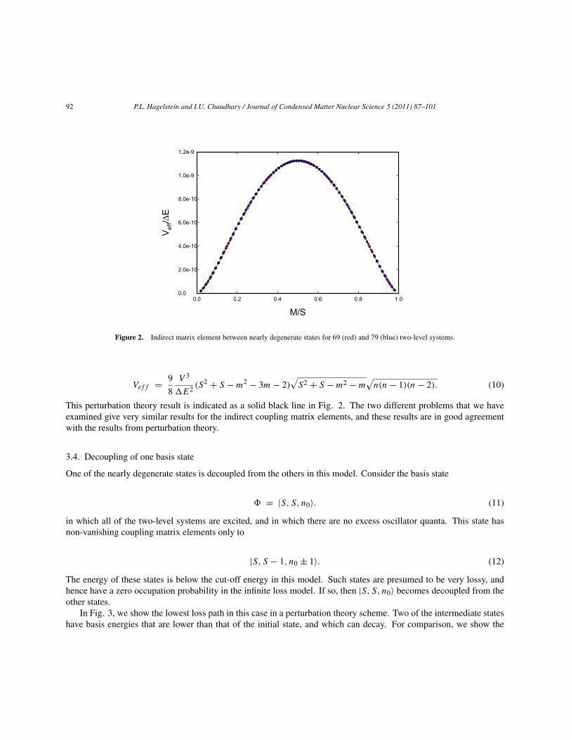
92 P.L. Hagelstein and I.U. Chaudhary / Journal of Condensed Matter Nuclear Science 5 (2011) 87–101
M/S0.0 0.2 0.4 0.6 0.8 1.0
Vef
f/∆E
0.0
2.0e-10
4.0e-10
6.0e-10
8.0e-10
1.0e-9
1.2e-9
Figure 2. Indirect matrix element between nearly degenerate states for 69 (red) and 79 (blue) two-level systems.
Veff = 9
8
V 3
E2 (S2 + S −m2 − 3m− 2)
√S2 + S −m2 −m
√n(n− 1)(n− 2). (10)
This perturbation theory result is indicated as a solid black line in Fig. 2. The two different problems that we haveexamined give very similar results for the indirect coupling matrix elements, and these results are in good agreementwith the results from perturbation theory.
3.4. Decoupling of one basis state
One of the nearly degenerate states is decoupled from the others in this model. Consider the basis state
= |S, S, n0〉. (11)
in which all of the two-level systems are excited, and in which there are no excess oscillator quanta. This state hasnon-vanishing coupling matrix elements only to
|S, S − 1, n0 ± 1〉. (12)
The energy of these states is below the cut-off energy in this model. Such states are presumed to be very lossy, andhence have a zero occupation probability in the infinite loss model. If so, then |S, S, n0〉 becomes decoupled from theother states.
In Fig. 3, we show the lowest loss path in this case in a perturbation theory scheme. Two of the intermediate stateshave basis energies that are lower than that of the initial state, and which can decay. For comparison, we show the

P.L. Hagelstein and I.U. Chaudhary / Journal of Condensed Matter Nuclear Science 5 (2011) 87–101 93
|S,n⟩
|S-1,n+1⟩
|S,n+2⟩
|S-1,n+3⟩
|S,n+4⟩
|S-1,n+5⟩E
Figure 3. Levels and transitions for lowest loss pathway in perturbation theory starting from |S, S, n〉 = |S, n〉, in the case of E = 5hω0.
lowest loss path in the general case in Fig. 4. In this case, none of the intermediate states have basis energies belowthat of the initial state, so that decay processes are minimized.
Coupling from this state in finite loss models would by necessity involve coupling through a lossy intermediatestate. This is the first time in the present discussion that we come across this issue. When we consider more complicatedmodels in papers that follow, we will find that this effect occurs generally in models of interest to us. We will eventuallyconnect this effect with the low-level emission of energetic particles that is seen in some Fleischmann–Pons experiments.
3.5. Discussion
The specific problem that we selected to focus on in this section appears now to be very simple to understand. Thesecond-order Hamiltonian leads to basis state energies that are very close to parabolic in m under conditions whereperturbation theory is valid. The coupling between neighboring nearly degenerate states is dominant, and closelymatches the result from perturbation theory.
In order for the associated system to exchange energy between the two degrees of freedom efficiently, all that we needis for the coupling matrix element between neighboring states to be as large as the splitting between neighboring states orgreater. In this model, it seems clear how to do it. The more two-level systems that we have, the smaller the interactionwe choose (in the scaling outlined above), so the smaller the difference between neighboring states. The couplingbetween neighboring states is strongest when about half of the two-level systems are excited, and is approximatelyconstant with the number of two-level systems when scaled as above. Hence, as there are more two-level systems, weare able to maintain coherence over a larger fraction of the Dicke states.

94 P.L. Hagelstein and I.U. Chaudhary / Journal of Condensed Matter Nuclear Science 5 (2011) 87–101
|m,n⟩
|m+1,n+1⟩
|m,n+2⟩
|m-1,n+3⟩
|m,n+4⟩
|m-1,n+5⟩E
Figure 4. Levels and transitions for lowest loss pathway in perturbation theory starting from |S,m, n〉 = |m, n〉, in the case of E = 5hω0.
4. Practical Issues
The isolation of a set of nearly degenerate states as outlined above is a very useful way to think about the problem, andprovides a way to compute the important parameters of the model. However, as we start to go further in this direction,new issues arise. There is a practical computational issue concerning how to determine the energy eigenvalue self-consistently, since it appears in the second-order Hamiltonian. The self-energy shift tends to split the nearly degeneratestates, so that we would like to understand under what conditions energy exchange can occur. The self-energy shift inaddition impacts our selection of basis states, which motivates us to consider a restricted basis approximation.
4.1. Solving the second-order eigenvalue problem
If the dimensionless coupling strength is small, then the self-energy is also small, which means that one can obtainsolutions to the second-order eigenvalue equation
Ec = Ha · c + Vab · (E − Hb)−1 · Vba · c (13)
by using the unperturbed basis state energy on the right hand side. When the self-energy begins to become significant,then the accuracy of the energy eigenvalues computed this way is degraded. We can obtain accurate results by solvingfor the energy eigenvalue self-consistently, as discussed in Appendix B.
Unfortunately, it quickly becomes inconvenient to obtain numerical solutions using this approach as the numberof quanta exchanged becomes larger, and when the dimensionless coupling strength is near or above unity. This willmotivate us to pursue an approximate solution to the problem, which we will consider below.

P.L. Hagelstein and I.U. Chaudhary / Journal of Condensed Matter Nuclear Science 5 (2011) 87–101 95
4.2. Constraint for maintaining coherence
From the results in the previous section, we have seen that models with the same maximum dimensionless couplingcoefficient g are very similar in terms of their self-energy and indirect coupling matrix elements. We can think ofa family of models where the maximum dimensionless coupling constant is held fixed, and the number of two-levelsystems is varied (assuming that n is kept constant and large). For this family of models, the self-energy and indirectcoupling matrix elements as a function of M/S are nearly the same. However, if the states were initially degenerate,then the splitting of the states is reduced when we have more two-level systems.
When we considered the dynamics resulting from the coupling between nearly degenerate states, we found that theproblem was simplest in the case of degenerate basis states. If there is a splitting between the states, then this can alterthe dynamics. In order for energy exchange to proceed at rates close to that for the degenerate version of the problem,we require that the splitting be less that the indirect coupling
|Em+1 − Em| < |Vm+ 12| (14)
in the notation of the previous paper. If the basis states are initially degenerate, then the splitting of interest for thisconstraint will be due to the self-energy shift. In this case, as we increase the number of two-level systems, the splittingwill decrease, and more of the nearly degenerate states will be able to participate in the dynamics.
4.3. Constraint for three-quantum exchange
We can develop an approximate version of the constraint in the special case of three quantum exchange that we discussedabove. The self-energy shift for small g is approximately
Em = − 0.0237 (maxg)2[
1 −(mS
)2]E (15)
so that
|Em+1 − Em| = 0.0237 (maxg)2(
2|m|S2
)E. (16)
The matrix element for indirect coupling from perturbation theory is approximately
Veff = 9
8(maxg)3
[1 −
(mS
)2]3/2
E (17)
in the limit that S and n are large. We can combine these estimates to obtain
∣∣∣mS
∣∣∣[
1 −(mS
)2]3/2 < 23.7 maxgS. (18)
This constraint is illustrated in Fig. 5.

96 P.L. Hagelstein and I.U. Chaudhary / Journal of Condensed Matter Nuclear Science 5 (2011) 87–101
maxg S0.001 0.01 0.1 1 10
|m/S
|
0.0
0.2
0.4
0.6
0.8
1.0
Figure 5. Evaluation of the constraint (18) in the case of three quantum exchange. The region in gray is where the level splitting is less than theindirect coupling matrix element.
4.4. Self-energy as potential energy of the coupled system
When the self-energy becomes large, there can be a significant shift of the energy levels. For example, when thecoupling is near unity, the self-energy can be on the order of E. Since this self-energy seems to be large, we need tothink some about what it means, and what the implications are for our approximation.
The self-energy comes about due to the interactions in the model that produces the coupling between the states.Perhaps it is best to think of it as a binding energy or equivalently, a potential energy, for the coupled systems. If so,then it may be best to think of it on a per two-level system basis, especially if n is very large. For large g the self-energybecomes linear in g, so that this point of view will be helpful much later on when we consider models which seekto describe the Fleischmann–Pons excess power effect. Under the conditions that we have encountered so far, thisself-energy per two-level system is small compared to the transition energy E. It can be substantial compared to theoscillator energy, especially when a large number of oscillator quanta are exchanged.
4.5. Fixed basis state model
In the lossy spin-boson model with infinite loss, we proposed that all states with an energy less than E were to beassumed to have infinite loss. If the self-energy is small, then the basis state energy will not be so different from thediagonal energy in the second-order H(E) matrix. Hence, in this limit the choice of which states to keep and which toomit is clear.
However, if we include the self-energy, then things become more complicated. If we omit all states with an energyless than some energy E, and then calculate the diagonal energies for the H(E) matrix, we will find that many of theresulting states have an energy less than the energy E which we selected as a cut-off due to the contribution of theself-energy. If the dimensionless coupling constant g is close to unity, this contribution can be very large.
One approach to this problem is to go back and revise the list of included and omitted states so as to be self consistentwith a cut-off energy. Another approach to the problem is to fix the basis initially, and keep it throughout the calculation.This latter approach is much more convenient for numerical calculations. In the limit that there are many oscillatorquanta exchanged for each two-level transition, then this kind of model will lead to minor errors locally in the list of

P.L. Hagelstein and I.U. Chaudhary / Journal of Condensed Matter Nuclear Science 5 (2011) 87–101 97
g0.03 0.05 0.07 0.2 0.3 0.5 0.70.1 1
Vef
f/∆E
10-5
10-4
10-3
10-2
10-1
100perturbation
theory
exact
Figure 6. Largest normalized effective indirect coupling matrix element Veff/E as a function of g computed using S = 19 (blue); perturbationtheory result (black). The number of oscillator quanta used in this calculation is 1012.
states that are retained (it will keep too many). We would not expect this to lead to significant changes in the modelparameters or dynamics, but we have not pursued this issue in our work.
In Fig. 6, we show results from such a computation for the largest indirect coupling matrix element as a functionof g. In most of the calculations that will follow in this and in following papers, we will work with this kind of model.
5. Discussion and Conclusions
In a previous paper of this set [17], we introduced the lossy spin-boson model and showed that it was capable of greatlyenhanced coherent energy exchange (as compared to the lossless spin-boson model) when many oscillator quanta areexchanged for a two-level system quantum. In this we are pleased that the new model is capable of such efficientcoherent energy exchange, since it is the basic effect that in our view is needed to account for excess heat in theFleischmann–Pons experiment.
However, it is clear that we are going to need much stronger analytical tools to obtain results in a relevant regime.Perturbation theory is helpful when the coupling is weak, but we are going to need the model to work in a very strongcoupling limit in order to convert a single two-level system quantum into 108 oscillator quanta. As a result, we need todevelop models and approximations which are useful in the strong coupling limit.
The second-order formulation that we introduced above allows us to extend our modeling well beyond the weakcoupling limit. We can use it directly to analyze the lossy spin-boson model when a relatively small number ofoscillator quanta are exchanged. This is useful since it allows us to discuss scaling for this model, and also to introducethe dimensionless coupling constant g.
We cannot use the second-order formulation presented here for direct calculations of models in which millions of

98 P.L. Hagelstein and I.U. Chaudhary / Journal of Condensed Matter Nuclear Science 5 (2011) 87–101
quanta are exchanged for each two-level system transition, since the approach does not scale well as a computationalproblem. What is important here is the notion that we can isolate the nearly degenerate states, and that the self-energyand the matrix elements for indirect coupling between nearest neighbors obey scaling laws. For example, even thoughwe are not able to perform a computation with 1010 two-level systems, we would have no trouble developing accurateestimates for the self-energy and indirect coupling between nearest neighbors for weak and moderately strong couplingin the case of 3 or 5 quantum exchange because of the scaling law. We still need to develop a scaling law that governs theself-energy and indirect coupling matrix element in the limit where a large number of oscillator quanta are exchanged.
In a paper that follows, we will present an approximation scheme which is based on the formulation presented herethat will allow us to perform calculations for models where a much larger number of oscillator quanta are exchanged.Based on these results we will be able to deduce a scaling law that is useful generally when the number of oscillatorquanta exchanged is large.
Appendix A. Numerical issues
The algebraic problem as outlined in Section 2 seems completely straightforward, but there are significant issues thatremain. Some of these concern numerical issues which we must face when implementing the approximation. We willprovide a brief discussion of a simple numerical approach in the subsections that follow.
Appendix A.1. Selection of basis states
We first consider the selection of basis states. We have the parity selection rule that states with positive parity (−1)n+mdo not couple with states with negative (−1)n+m. So, we have chosen to work with positive parity states here.
Next, we note that the number of Dicke states associated with the two-level systems alone is 2S + 1, since all ofthe two-level systems can be in the ground state (m = −S) and all of them can be in the excited state (m = S). Theline for equal energy is defined according to
E = Em+ hω0n. (A.1)
It seems reasonable to keep states up to some fixed energy above the threshold energy, which we define here has being
E0 = ES + hω0n0. (A.2)
At this energy, all of the two-level systems are excited, and the oscillator has nominal excitation n0.
Appendix A.2. Banded Cholesky decomposition
In the algebraic equation above, we need to compute the inverse of a matrix. While this seems straightforward, not allnumerical algorithms will result in a symmetric inverse. Consequently, we need to pay some attention to how this iscarried out.
To proceed, we define
A = A(E) = Hb − E. (A.3)
Since A is symmetric, LU decomposition can be carried out using

P.L. Hagelstein and I.U. Chaudhary / Journal of Condensed Matter Nuclear Science 5 (2011) 87–101 99
A = L · LT, (A.4)
where L is lower triangular.We can use Cholesky decomposition in order to decompose A. This algorithm seems to work pretty well for this
problem. We are aided by the fact that A is banded, which speeds the computation of L, and leads to a banded matrixL. Even for a very large problem, we are able to compute L by Cholesky decomposition conveniently.
Appendix A.3. Matrix inverse of the lower triangular matrix
For the solution linear systems, Cholesky decomposition is the time-consuming part of the algorithm in the case ofsymmetric matrices. Determination of the solution is done by back substitution. We have tried various algorithmsbased on back substitution, however, it seemed useful along the way to carry out an explicit construction of the inverse,and we subsequently kept it.
The construction of the inverse of a lower triangular matrix can be done reasonably efficiently in the case of a bandedmatrix. The algorithm that we have used works as follows. We assume that the inverse is also a lower triangular matrixB, so that
B · L = I. (A.5)
To understand the associated algorithm for determining B, it is useful to write this equation out explicitly in the case of3 × 3 matrices. We may write
⎛⎝B11 0 0B21 B22 0B31 B32 B33
⎞⎠ ·
⎛⎝L11 0 0L21 L22 0L31 L32 L33
⎞⎠ =
⎛⎝
B11L11 0 0B21L11 + B22L21 B22L22 0
B31L11 + B32L21 + B33L31 B32L22 + B33L32 B33L33
⎞⎠ . (A.6)
It seems clear that we can solve for diagonal terms directly using
Bii = 1
Lii. (A.7)
If we go off of the diagonal by one, we end up with equations of the form
Bi,i−1Li−1,i−1 + BiiLi,i−1 = 0. (A.8)
We can solve this using
Bi,i−1 = − BiiLi,i−1
Li−1,i−1. (A.9)
It is possible to continue the algorithm to determine the different Bij values based on a knowledge of known L andpreviously determined B matrix elements.

100 P.L. Hagelstein and I.U. Chaudhary / Journal of Condensed Matter Nuclear Science 5 (2011) 87–101
Appendix A.4. Construction of the second-order matrix
The second-order matrix can be written as
H(E) = Ha − Vab · A−1(E) · Vba. (A.10)
This can be written in terms of L as
H(E) = Ha − Vab · (L · LT)−1 · Vba = Ha − Vab · (LT)−1 · L−1 · Vba. (A.11)
We can recast this as
H(E) = Ha − (L−1 · Vba)T · (L−1 · Vba). (A.12)
In this form, the resulting second-order matrix is explicitly real and symmetric, which was one of the goals of ourconstruction.
Appendix B. Self-consistent computation of the energy
The Schrödinger equation in the case of the second-order Hamiltonian can be written as
Ec = Ha · c + Vab · (E − Hb)−1 · Vba · c. (B.1)
We see that the energy eigenvalue appears both on the right-hand side (RHS) and on the left-hand side (LHS) of thisequation. If the self-energy shift is small, then we can approximate the energy on the RHS with the basis state energyand obtain good results. If the self-energy shift is large, then a self-consistent calculation is needed.
Appendix B.1. Simple iteration
Iterative schemes can be used to obtain a self-consistent solution. The simplest iterative scheme can be written as
E(k+1)c = Ha · c + Vab · (E(k)j − Hb)−1 · Vba · c. (B.2)
On the LHS, we have the energy eigenvalue in generalE(k+1) for the k+1 iteration; on the RHS we have one particularbasis state energy Ekj determined on the previous iteration. If the scheme converges, then it can be stopped when thechange in the energy eigenvalue of the state of interest doesn’t change any more
|E(k+1)j − E
(k)j | < ε. (B.3)
The iterations can be started by taking the initial energy equal to the initial basis state energy.

P.L. Hagelstein and I.U. Chaudhary / Journal of Condensed Matter Nuclear Science 5 (2011) 87–101 101
Appendix B.2. Iterations with relaxation
We have found that the iterations described above do not converge when the dimensionless coupling coefficient ap-proaches unity. In this case, we have been able to converge using a modification of the scheme with relaxation basedon
E(k+1)c = Ha · c + Vab · (F (k)j − Hb)−1 · Vba · c, (B.4)
where
F(k)j = aE
(k)j + (1 − a)E
(k−1)j (B.5)
with a taken to be near 0.2.
References
[1] P.L. Hagelstein, A unified model for anomalies in metal deuterides, Proc. ICCF9, 2002, p. 121.[2] P.L. Hagelstein and I.U. Chaudhary, Progress on phonon exchange models for excess heat in metal deuterides, Proc. 13th Int.
Conf. Cold Fusion, 2007, p. 590.[3] P.L. Hagelstein and I.U. Chaudhary, Models relevant to excess heat production in Fleischmann–Pons experiments, Low-energy
nuclear reactions sourcebook, ACS Symposium Series 998, 2008, p. 249.[4] P.L. Hagelstein and I.U. Chaudhary, Excitation transfer and energy exchange processes for modeling the Fleischmann–Pons
excess heat effect, Proc. 14th Int. Conf. Cold Fusion, 2008, p. 579.[5] M. Fleischmann, S. Pons and M. Hawkins, J. Electroanal Chem. 201 (1989) 301; errata 263 (1990) 187.[6] M. Fleischmann, S. Pons, M.W. Anderson, L.J. Li and M. Hawkins, J. Electroanal. Chem. 287 (1990) 293.[7] M.C.H. McKubre, S. Crouch-Baker, R.C. Rocha-Filho, S.I. Smedley, F.L. Tanzella, T.O. Passell, J. Santucci, J. Electroanal.
Chem. 368 (1994) 55.[8] E. Storms, Science of Low Energy Nuclear Reaction: A comprehensive compilation of evidence and explanations about cold
fusion, World Scientific, Singapore, 2007.[9] M.H. Miles, R.A. Hollins, B.F. Bush, J.J. Lagowski, R.E. Miles, J. Electroanal. Chem. 346 (1993) 99.[10] M. H. Miles, B. F. Bush, and J. J. Lagowski, Fusion Technology 25 (1994) 478.[11] M.H. Miles, Correlation of excess enthalpy and helium-4 production: A review, Proc. 10th Int. Conf. Cold Fusion, 2003, p.
123.[12] P.L. Hagelstein, Naturwissenschaften 97 (2010) 345.[13] P L. Hagelstein, M.C.H. McKubre, D.J. Nagel, T.A. Chubb, R.J. Hekman, New physical effects in metal deuterides, Proc. 11th
Int. Conf. Cold Fusion, 2005, p. 23.[14] F. Bloch and A. Siegert, Phys. Rev. 57 (1940) 522.[15] J. Shirley, Phys. Rev. 138 (1965) B979.[16] C. Cohen-Tannoudji, J. Dupont-Roc and C. Fabre, J. Phys. B: Atom. Molec. Phys. 6 (1973) L214.[17] P.L. Hagelstein and I.U. Chaudhary, Energy exchange in the lossy spin-boson model, J. Cond. Mat. Nucl. Sci. 5 (2011) 52.[18] P.L. Hagelstein and I.U. Chaudhary, Dynamics in the case of coupled degenerate states, J. Cond. Mat. Nucl. Sci. 5 (2011) 72.[19] P.L. Hagelstein and I.U. Chaudhary, J. Phys. B: Atom. Molec. Phys. 41 (2008) 035601.[20] P.L. Hagelstein and I.U. Chaudhary, J. Phys. B: Atom. Molec. Phys. 41 (2008) 035602.

J. Condensed Matter Nucl. Sci. 5 (2011) 102–115
Research Article
Local Approximation for the Lossy Spin–boson Model
Peter L. Hagelstein ∗Research Laboratory of Electronics, Massachusetts Institute of Technology, Cambridge, MA 02139, USA
Irfan U. ChaudharyDepartment of Computer Science and Engineering, University of Engineering and Technology. Lahore, Pakistan
Abstract
We are interested in the problem of coherent energy exchange in the spin-boson model augmented with loss, in the limit of infiniteloss. This model is interesting because it predicts rapid coherent energy exchange under conditions when the transition energy ofthe two-level systems is much greater than the characteristic energy of the oscillator. Here we introduce the local approximation,in which we assume that the matrix elements change little when an energy exchange event occurs. This approximation results ina periodic system when a resonance condition is satisfied, which is much easier to solve than the original problem. We consider amodel problem where we analyze the self-energy and indirect coupling matrix elements numerically and in the local approximation,with good agreement. Systematic results from the local approximation are obtained for the self-energy and indirect coupling matrixelements in models where 3, 5, 7, 9, and 11 quanta are exchanged.© 2011 ISCMNS. All rights reserved.
Keywords: Coherent energy exchange, Excess heat, Fleischmann–Pons experiment, Lossy spin-boson model, Theory
1. Introduction
There have been a great many experiments which indicate that excess energy is produced in the Fleischmann–Ponsexperiment [1,2] and its variants. The amount of energy observed in some of these experiments is prodigious, with noobvious commensurate chemical processes observed. Since there has been measured 4He in amounts proportional to theenergy produced [3–5], with an associatedQ-value near 24 MeV [6], one possible conclusion is that there is some kind ofnew nuclear reaction process occurring. The conundrum that arises in such a proposal is that known exothermic nuclearreactions put the reaction energy into energetic nuclear particles. In the Fleischmann–Pons experiment, there simplyaren’t energetic nuclear particles in amounts commensurate with the energy produced [7]. Consequently, conventional
∗E-mail: [email protected]
© 2011 ISCMNS. All rights reserved.

P.L. Hagelstein and I.U. Chaudhary / Journal of Condensed Matter Nuclear Science 5 (2011) 102–115 103
nuclear reactions that appear in the nuclear physics literature in general cannot be candidates to account for the excessheat effect.
If so, then the question arises as to what reactions or new physical processes can be consistent with these experimentalobservations? It seems the outstanding theoretical problem which must be faced involves the conversion of a very largeMeV-level nuclear quantum of energy into a very large number of eV-level or meV-level quanta.
If we adopt such a point of view, then the recent results from two-laser experiments [8,9] perhaps begin to makesense. Excess power is observed when the cathode is stimulated by two weak laser beams, and the response dependson the frequency difference between the two laser frequencies. Two of the frequencies at which strong responses areobserved correspond to the -point (8 THz) and L-point (15 THz) of the optical phonon mode dispersion curve of PdD.The excess power in these experiments is seen in many cases to persist when the lasers are turned off. Some poweris put into one of the these modes by the lasers, which initially stimulates excess power production. If excess powercontinues when the lasers are turned off, we might infer that some of the energy which is being produced in the reactionis going into the mode that has been stimulated. This could be verified by Raman measurements, but such experimentshave not yet been attempted.
From experiment, a picture seems to emerge in which a new kind of nuclear reaction process occurs, in whichthe reaction energy is communicated to the optical phonon modes. Such an effect is unprecedented, which makes thetheoretical problem of model development that much harder. Nevertheless, we have managed to construct new modelsbased on two-level systems coupled to an oscillator, which exhibit a much accelerated coherent energy exchange effectinvolving the fractionation of a large energy quantum into a great many low energy quanta.
The simplest version of the model is the spin-boson model augmented with loss, which we have introduced in earlierpublications. We have demonstrated the new coherent energy exchange effect using perturbation theory [10], and wehave also presented a second-order formulation of the model [11] which allows us to think about the model in terms ofa set of ordered nearly degenerate states with nearest neighbor coupling. In these papers, we have begun the analysisof the model, introducing tools that help us understand and analyze important properties. Our goal ultimately is tounderstand how coherent energy exchange works in a regime relevant to the Fleischmann–Pons experiment, and in thiswork we take a big step in that direction. In this paper, we introduce the local approximation, which provides us witha powerful tool to analyze coherent energy exchange when the coupling is strong, and also when a larger number ofoscillator quanta are exchanged.
2. Local Approximation for the Lossy Spin-boson Model
As we have discussed in earlier works, the lossy spin-boson model is described by the Hamiltonian [10]
H = ESz
h+ hω0a
†a + V (a† + a)2Sxh
− ih
2(E), (1)
where E is the transition energy of the two-level systems, where hω0 is the oscillator energy, and where V is thecoupling strength. Loss is included through the second-order −ih(E)/2 term that comes from a Brillouin–Wignerformulation (see [10]). Eigenfunctions of the coupled two-level systems and oscillator can be found from the solutionof the eigenvalue problem
E = H. (2)

104 P.L. Hagelstein and I.U. Chaudhary / Journal of Condensed Matter Nuclear Science 5 (2011) 102–115
2.1. Finite basis approximation
We can make use of a finite basis approximation for the associated wave function in terms of product basis statesaccording to
=∑m
∑n
cm,n|S,m〉|n〉. (3)
We can use this to develop the above eigenvalue equation in terms of the expansion coefficients according to
Ecm,n =(Em+ hω0n− i
h
2(E)
)cm,n + V
√n+ 1
√(S −m)(S +m+ 1)cm+1,n+1
+ V√n√(S −m)(S +m+ 1)cm+1,n−1 + V
√n+ 1
√(S +m)(S −m+ 1)cm−1,n+1
+ V√n√(S +m)(S −m+ 1)cm−1,n−1. (4)
2.2. Limit of many oscillator quanta and two-level systems
In the event that n is very large, then
√n+ 1 ≈ √
n. (5)
If S is very large, and if m is not close to ±S, then√(S −m)(S +m+ 1) ≈
√S2 −m2,
√(S +m)(S −m+ 1) ≈
√S2 −m2 (6)
Under these approximations, the coupling coefficients to the nearby states are the same, so that the eigenvalue equationfor the expansion coefficients is approximately
Ecm,n =[Em+ hω0n− i
h
2(E)
]cm,n
+ V√n√S2 −m2
(cm+1,n+1 + cm+1,n−1 + cm−1,n+1 + cm−1,n−1
). (7)
2.3. Local approximation in terms of g
We recall that the dimensionless coupling constant g is given by
g = V√n√S2 −m2
E. (8)
The approximate eigenvalue equation can be written in terms of the dimensionless coupling constant as
E
Ecm,n =
(1 + hω0
E− i
h(E)
2E
)cm,n
+ g
(cm+1,n+1 + cm+1,n−1 + cm−1,n+1 + cm−1,n−1
). (9)

P.L. Hagelstein and I.U. Chaudhary / Journal of Condensed Matter Nuclear Science 5 (2011) 102–115 105
Althoughg is dependent onm, we can simplify the problem significantly if we consider it to be a constant. The eigenvalueequation that results constitutes a local approximation, allowing us to obtain approximate basis state energies and indirectcoupling coefficients.
2.4. Hamiltonian associated with the local approximation
We can write down a Hamiltonian for this local approximation as
H = ESz
h+ hω0a
†a + gE
(δn+ + δn−
)(δm+ + δm−
)− i
h
2(E), (10)
where the δ operators satisfy
δn±|n〉 = |n± 1〉, (11)
δm±|S,m〉 = |S,m± 1〉. (12)
3. Periodicity
An important feature of the Hamiltonian in the local approximation is that it is invariant under translations of the form
T±|S,m〉|n〉 = |S,m± 1〉|n∓n〉, (13)
when the resonance condition holds
E = n hω0 (14)
for odd n.
3.1. Bloch’s theorem
The Hamiltonian is invariant under the energy-preserving translations of the T± operators, so we know that Bloch’stheorem applies. The eigenfunctionsm,n of the local Hamiltonian satisfy the time-independent Schrödinger equation
Hm,n = Em,n. (15)
In the local approximation with odd integer n, the Hamiltonian commutes with the translation operators
[T±, H ] = 0. (16)
Hence it is possible to find solutions which are eigenfunctions of both operators
Hm,n = Em,n, (17)

106 P.L. Hagelstein and I.U. Chaudhary / Journal of Condensed Matter Nuclear Science 5 (2011) 102–115
|m,n⟩
|m,n+2⟩
|m,n+4⟩
|m,n+6⟩
|m+1,n-∆n⟩
|m+1,n-∆n+2⟩
|m+1,n-∆n+4⟩
|m+1,n-∆n+6⟩
|m-1,n+∆n⟩
|m-1,n+∆n+2⟩
|m-1,n+∆n+4⟩
|m-1,n+∆n+6⟩
m
n+m∆n
Figure 1. Levels and selected couplings in m and n+mn basis with n = 5, plotted using m and n+mn (proportional to the energy) axes.State |m, n+ 6〉 is coupled to higher energy states |m+ 1, n+ 6 ± 1〉, although this coupling is not shown.
T+m,n = Cm,n. (18)
These solutions can be written in the form
m,n = eimφum,n, (19)
where the um,n are periodic in m. As a result, the energy eigenvalues can be described as a set of bands in φ from theeigenvalue equation
E(φ)eimφum,n = Heimφum,n. (20)
3.2. Reduced problem and boundary conditions
Since the problem is periodic under the local Hamiltonian, we can reduce the problem by working with a single columnof states such as plotted in Fig. 1. We need only include the states |m, n〉, |m, n+ 2〉, · · · explicitly. The phase factorsthat result in the Bloch solution relate the phase of a basis state with one value of m to the phase of the basis stateat the same energy at a neighboring value of m. So, a Bloch state solution can be developed from a set of expansioncoefficients associated with the basis states in a single column, knowing that the expansion coefficients for the basisstates in neighboring columns differ only by a single phase factor for each column.

P.L. Hagelstein and I.U. Chaudhary / Journal of Condensed Matter Nuclear Science 5 (2011) 102–115 107
4. Product solution
The discussion above suggests that a convenient product solution can be constructed using
=∑m
∑n
dmvn+mn|S,m〉|n+mn〉 (21)
assuming large S with m away from ±S, and large n. Since the index of the v coefficients is proportional to the basisstate energy, it is unaffected by T± translations. Hence we can implement the phase factors associated with the Blochstates in the dm coefficients by taking
dm = eimφ. (22)
The local Hamiltonian couples states with m and n indices that differ by one unit; however, when we line the states upaccording to their energy (which is useful in the local approximation), then this coupling appears to connect relativelydistant states as indicated in Fig. 1.
4.1. Self-energy
Starting with the basis expansion above, we can isolate the v coefficients by taking advantage of orthogonality
〈m′, n′|m, n〉 = δm′,mδn′,n. (23)
The eigenvalue equation associated with the expansion coefficients can be written as
E(φ)dmvn+mn =[Em+ nhω0 − i
h
2(E)
]dmvn+mn
+ gE
[dm+1(vn+1+(m+1)n + vn−1+(m+1)n)
+ dm−1(vn+1+(m−1)n + vn−1+(m−1)n)
]. (24)
If we focus on the coefficients corresponding to the column with m = 0 and use dm = exp(imφ), we obtain
E(φ)vn =[nhω0 − i
h
2(E)
]vn
+ gE
[eiφ(vn+n+1 + vn+n−1)+ e−iφ(vn−n+1 + vn−n−1)
]. (25)
The lowest energy solution of this eigenvalue equation gives the self-energy in the local approximation.
4.2. Indirect coupling matrix element
Under conditions that are of interest to us in the development of models relevant to the excess heat effect in theFleischmann–Pons experiment, the indirect coupling between nearly degenerate states is weak. In the local approx-imation, a second-order formulation that isolates the nearly degenerate states would result in degenerate states whenn is an odd integer. The associated eigenvalue equation is of the form

108 P.L. Hagelstein and I.U. Chaudhary / Journal of Condensed Matter Nuclear Science 5 (2011) 102–115
g0.00 0.02 0.04 0.06 0.08 0.10
E(g
)/∆E
-0.025
-0.020
-0.015
-0.010
-0.005
0.000
Figure 2. Self-energies for the nearly degenerate basis states of the test problem (black circles) and for the local approximation (blue line).
Edm = E0dm + Veff(dm−1 + dm+1). (26)
It is possible to obtain a useful version of such an equation from the model under consideration above (but this will beof more interest in a later paper, so we defer the associated discussion).
We can solve this equation using
dm = eimφ (27)
consistent with the phase factor that we used above from Bloch’s theorem. The associated energy eigenvalue is
E(φ) = E0 + 2Veff cosφ. (28)
As a result, if we were to solve the eigenvalue equation in the local approximation for two values of φ, then we coulddetermine the indirect coupling coefficient in the weak coupling approximation. For example, if we take φ values of 0and π , then we obtain
E(0)− E(π) = 4Veff. (29)
We have used this to obtain numerical estimates for the indirect coupling matrix element for the restricted basis versionof the infinite loss model with success.

P.L. Hagelstein and I.U. Chaudhary / Journal of Condensed Matter Nuclear Science 5 (2011) 102–115 109
g0.02 0.03 0.04 0.05 0.06 0.07 0.08 0.09 0.1
Vef
f(g)/∆
E
1e-8
1e-7
1e-6
1e-5
1e-4
Figure 3. Indirect coupling matrix elements for the nearly degenerate basis states of the test problem (black circles) and for the local approximation(blue line).
5. Model Problem
The local approximation described above allows us to develop approximate results for the self-energy and indirectcoupling matrix elements for the lossy spin-boson model. Since it is an approximation, we are interested in whetherit can give good results. To explore this, we developed a model problem in which we can compare the approximateresults with exact numerical results.
5.1. Problem specification
For the test problem, we chose
E
hω0= 5 (30)
with
S = 19.5, (31)
which corresponds to 39 two-level systems. We took the coupling strength V to satisfy
V√nS
E= 0.1 (32)
for which the maximum dimensionless coupling strength g is close to 0.10. We have taken the lossy spin-boson modelin the limit of infinite loss, using a restricted basis approximation [11].

110 P.L. Hagelstein and I.U. Chaudhary / Journal of Condensed Matter Nuclear Science 5 (2011) 102–115
g0.01 0.1 1 10
-E/∆
E
10-4
10-3
10-2
10-1
100
101
102
Figure 4. Self-energy as a function of g for n = 3,5,7,9,11 (n = 3 is the bottom curve, and n = 11 is the top).
5.2. Second-order formulation
In a previous paper we described a second-order formulation for the lossy spin-boson problem [11]. The advantage ofthis formulation is that we are able to reduce the original complicated Hamiltonian into a conceptually simpler one thatfocuses on a set of nearly degenerate states that are coupled indirectly. This formulation can be represented throughthe second-order Hamiltonian
H(E) = Ha + Vab · (E − Hb)−1 · Vba, (33)
which we can evaluate numerically to determine the self-energies and indirect matrix elements.For this calculation, we took 50 energy points for the energy in the denominator and evaluated the self-energies
and indirect coupling matrix elements between nearest neighbors. Then we interpolated for self-consistency for eachstate to get the self-energies. Based on this interpolation we obtained accurate values for the indirect coupling matrixelements.
5.3. Comparison of the self-energy
To compare the results from the two models, we needed to develop an estimate for the local coupling strength. Ourprocedure was to sum the coupling matrix elements out of one of the initial degenerate basis states of the original fullHamiltonian, and then divide by the product of E and the number of couplings. This produces an approximate localg defined by

P.L. Hagelstein and I.U. Chaudhary / Journal of Condensed Matter Nuclear Science 5 (2011) 102–115 111
φ
0.0 0.5 1.0 1.5 2.0 2.5 3.0
[E(0
)-E(φ
)]/[E
(0)-E
(π)]
0.0
0.2
0.4
0.6
0.8
1.0
Figure 5. Relative self-energy as a function of phase angle φ for n = 5. Weak coupling limit is the lower curve in black; results from bottom totop in blue are for g = 0.3, 1, 10.
gi =∑j Hij∑j E
, (34)
where the summation over j includes only states with non-zero coupling matrix elements from i. We plotted theself-energy for each state versus the approximate state gi as points in Fig. 2, and we also plotted results for the self-energy as a function of g in the local approximation as a line. As can be seen, the agreement is excellent for all of thenearly-degenerate basis states.
5.4. Comparison of the indirect coupling matrix elements
In Fig. 3, we plotted the indirect matrix elements from each state as for each dimensionless coupling strength gi aspoints, and results from the associated local approximation as a line. One sees good agreement for the larger valuesof g, which corresponds to the part of the problem where the different gi values vary slowly (where we would expectthe local approximation to be best). The agreement is not quite as good for the smaller gi values. This is because thecoupling matrix elements of the original Hamiltonian are most rapidly varying in this regime.
5.5. Discussion
We see from this comparison that the local approximation does very well in estimating the self-energy, which variesrelatively slowly with g. The indirect coupling matrix element is a much stronger function of g, so the local approx-imation does not do quite as well. The underlying approximation that the coupling matrix elements of the original

112 P.L. Hagelstein and I.U. Chaudhary / Journal of Condensed Matter Nuclear Science 5 (2011) 102–115
g0.01 0.1 1 10
Vef
fj /∆E
10-8
10-7
10-6
10-5
10-4
10-3
10-2
10-1
100
101
Figure 6. Indirect coupling matrix elements between nearest neighbors (upper curve); second, third and fourth nearest neighbors (lower curves indescending order).
Hamiltonian are all the same begins to break down for small g. In this regime, the indirect matrix elements whichcouple to states where the local coupling is stronger becomes larger, while the indirect matrix elements which coupleto states with weaker local coupling become smaller. In this regime, we see a splitting of the matrix elements for thetwo different directions (see Fig. 3). When this occurs, the indirect matrix elements from the local approximation liebetween them.
In this model problem, the number of two-level systems is not particularly large. As a result, we end up seeinga weak departure between the numerically exact results from the second-order formulation and the results from thelocal approximation. In problems where the number of two-level systems is much larger, we would expect the localapproximation to be much better, since the associated coupling matrix elements of the original problem generally willhave smaller differences locally.
6. Local Approximation Results
One advantage of the local approximation is that we are able to carry out computations systematically for a wide rangeof dimensionless coupling constants g when the number of oscillator quanta exchanged is modest.
6.1. Self-energies
In Fig. 4, we show the self-energies as a function of g for the local approximation for different values ofn. One seesthat for larger values of n, the different self-energies quickly approach a large n limit. For small g the self energyis quadratic in g; and for large g the self-energy is linear in g.

P.L. Hagelstein and I.U. Chaudhary / Journal of Condensed Matter Nuclear Science 5 (2011) 102–115 113
6.2. Energy as a function of angle
We expect the self-energy to be dependent on the phase angle φ, with a simple sinusoidal dependence when the couplingis weak as discussed above. In Fig. 5, we show results for the relative self-energy in the case of five quantum exchangefor different values of the dimensionless coupling constant g. When the coupling is very weak, nearest neighborcoupling is dominant, and
E(0)− E(φ)
E(0)− E(π)→ 1 − cosφ. (35)
We see that when g = 0.3 that the the relative self-energy is a good match, and that nearest neighbor coupling isdominant. For the larger values of the dimensionless coupling constant, there is some deviation from the cosinefunction, which indicates that coupling to second and higher neighbors contributes.
It is possible to extract from the angle-dependent self energy curves the coupling parameters for the differentneighbors systematically. We have done this for the results shown in Fig. 5 to obtain the indirect coupling coefficientsfor the different neighbors in Fig. 6. From these results we see that nearest-neighbor coupling dominates, and that asthe magnitude of the splitting gets larger the contributions from other neighbors increases.
6.3. Level splittings
Results for the normalized level splittings for different local approximation models as a function of g are shown inFig. 7. In the event that the indirect coupling is weak, this normalized level splitting approaches the indirect couplingmatrix element
g0.01 0.1 1 10
[E(0
)-E(π
)]/4∆
E
10-8
10-7
10-6
10-5
10-4
10-3
10-2
10-1
100
101
Figure 7. Normalized level splitting as a function of g for n = 3, 5, 7, 9, 11 (n = 3 is the top curve, and n = 11 is the bottom).

114 P.L. Hagelstein and I.U. Chaudhary / Journal of Condensed Matter Nuclear Science 5 (2011) 102–115
E(0)− E(π)
4→ Veff (36)
It is easiest to carry out systematic computations for the level splitting, without isolating the contributions of indirectcoupling between the different nearly degenerate neighbors.
In general, we see that the level splitting in the lossy spin-boson model decreases with the exchange of moreoscillator quanta, and that the curves become sharper with a threshold at increasing g as n increases.
7. Discussion and Conclusions
In previous papers we have provided a systematic presentation of the lossy spin-boson model, which we have beeninterested in because of it is capable of fast coherent multi-quantum energy exchange between two-level systems andan oscillator. Although the model Hamiltonian is relatively simple in form, the analysis of coherent energy transferbetween the two-level systems and the oscillator in the multi-quantum regime is not straightforward. In earlier work wehave explored coherent energy exchange using perturbation theory, and a formulation that is based on a second-orderHamiltonian. Using these tools, we can study coherent energy exchange when a few quanta are exchanged underconditions where the coupling is weak to moderate. Here we introduced the local approximation, which greatly extendsour ability to quantify coherent energy exchange in the model.
In the local approximation, we assume that the system is essentially unchanged when a single two-level systemgains or loses excitation, such that the underlying coupling matrix elements do not change. The assumption leads to aproblem that is periodic when the resonance condition is satisfied, and the resulting periodic problem is much easierto solve. We considered a model problem in order to see how good the local approximation does when compared toresults obtained from the second-order Hamiltonian. The results from the local approximation were found to be verygood under conditions where we would expect the local approximation to be good (large S, S2 −m2 >> 0).
Within the framework of the local approximation, we define a local value of the dimensionless coupling constantg, and the self-energy and indirect coupling matrix elements become unique functions of this g. We analyze the lossyspin-boson model in the limit of infinite loss, and the result of the analysis then is a determination of the associatedself-energy and indirect matrix element functions versus g for a particular value of n. In practice, it is simpler tocompute the level splitting E(0)−E(π) than the indirect coupling matrix elements. This is useful since we know thatnearest neighbor coupling dominates when the splitting is smaller than E.
We have given results for the self-energy and level splitting for different values ofn between 3 and 11 here. Theseresults allow us to see the general trends that emerge. For example, the self-energy is quadratic at low g and linearwhen g is large. As the number of quanta exchanged becomes large, the self-energy curve approaches a largen limit.The level splitting (and coherent energy exchange rate) becomes smaller when more quanta are exchanged, as we mightexpect since intuitively we would expect the corresponding physical system to have more trouble breaking up a bigquantum into smaller pieces.
What remains is for us to extend our analysis even further to understand what happens when n becomes large.From the results obtained so far, we would expect that g is going to have to become large in order to obtain a finite ratefor coherent energy exchange. As we shall see, the local approximation presented in this paper is going to be of greathelp in analyzing this limit; however, we are going to need additional tools in order to extract quantitative results fromthe local approximation in this limit. (which we will discuss in a subsequent paper).
References
[1] M. Fleischmann, S. Pons and M. Hawkins, J. Electroanal Chem., 201 (1989) 301; errata, 263 (1990) 187.

P.L. Hagelstein and I.U. Chaudhary / Journal of Condensed Matter Nuclear Science 5 (2011) 102–115 115
[2] M. Fleischmann, S. Pons, M.W. Anderson, L.J. Li and M. Hawkins, J. Electroanal. Chem., 287 (1990) 293.[3] M.H. Miles, R.A. Hollins, B.F. Bush, J.J. Lagowski, R.E. Miles, J. Electroanal. Chem. 346 (1993) 99.[4] M.H. Miles, B.F. Bush, and J.J. Lagowski, Fusion Technol. 25 (1994) 478.[5] M.H. Miles, Correlation of excess enthalpy and helium-4 production: A review, Proc. ICCF10, 2004, p. 123.[6] P.L. Hagelstein, M.C.H. McKubre, D.J. Nagel, T.A. Chubb, R.J. Hekman, New physical effects in metal deuterides, Proc.
ICCF11, 2005, p. 23.[7] P.L. Hagelstein, Naturwissenschaften 97 (2010) 345.[8] D. Letts, D. Cravens and P.L. Hagelstein, Dual laser stimulation and optical phonons in palladium deuteride, in low-energy
nuclear reactions and new energy technologies, Low-Energy Nuclear Reactions Sourcebook, Vol. 2, American Chemical Society,Washington, DC, 2009, p. 81.
[9] P.L. Hagelstein, D. Letts and D. Cravens, Terahertz difference frequency response of PdD in two-laser experiments, J. Cond.Mat. Nucl. Sci. 3 (2010) 59.
[10] P.L. Hagelstein and I.U. Chaudhary, Energy exchange in the lossy spin-boson model, J. Cond. Mat. Nucl. Sci. 5 (2011) 52.[11] P.L. Hagelstein and I.U. Chaudhary, Second-order formulation and scaling in the lossy spin-boson model, J. Cond. Mat. Nucl.
Sci. 5 (2011) 87.

J. Condensed Matter Nucl. Sci. 5 (2011) 116–139
Research Article
Coherent Energy Exchange in the Strong Coupling Limit of theLossy Spin-Boson Model
Peter L. Hagelstein ∗Research Laboratory of Electronics, Massachusetts Institute of Technology, Cambridge, MA 02139, USA
Irfan U. ChaudharyDepartment of Computer Science and Engineering, University of Engineering and Technology. Lahore, Pakistan
Abstract
We focus on the lossy spin-boson model since it is capable of efficient energy exchange between two-level systems and an oscillatorunder conditions where the characteristic energy of the oscillator is small compared to the transition energy of the two-level systems.We are considering this model as the essential component for a theoretical understanding of the excess heat effect in the Fleischmann–Pons experiment. We introduce an iterative algorithm that allows the numerical calculation of eigenfunctions and eigenvalues of thecoefficient eigenvalue equation that arises in the local approximation. From systematic calculations in the strong coupling limit weestablish scaling laws for the self-energy and for the indirect coupling matrix element in the local approximation. These results areused to study the system dynamics for simple strong coupling models.© 2011 ISCMNS. All rights reserved.
Keywords: Coherent energy exchange, Excess heat, Fleischmann–Pons experiment, Lossy spin-boson model, Theory
1. Introduction
In this work we continue our studies of coherent energy exchange between a set of two-level systems and an oscillator,under conditions where the transition energy of the two-level systems is much greater than the characteristic energyof the oscillator. Our interest in this problem is motivated by a great many experiments in which positive results havebeen reported on measurements of excess heat in the Fleischmann–Pons effect [1,2]. In these experiments a very largeamount of energy is sometimes produced, with no sign of chemical or material changes commensurate with the energyproduced. Fleischmann and Pons conjectured that the origin of the energy was nuclear; however, known exothermicnuclear reactions that produce energy do so through energetic particles, and there are no commensurate energetic
∗E-mail: [email protected]
© 2011 ISCMNS. All rights reserved.

P.L. Hagelstein and I.U. Chaudhary / Journal of Condensed Matter Nuclear Science 5 (2011) 116–139 117
particles in the Fleischmann–Pons experiment. Helium has been observed correlated with the energy [3–5], and theratio of energy produced to helium observed is near 24 MeV [6]. This is significant since it is consistent with the massdifference between two deuterons and a 4He nucleus.
Hence, experiment suggests that the energy is probably nuclear in origin, and that perhaps deuterons are somehowreacting to make 4He. The big problem with such a statement is that there are no previous examples in nuclearphysics of nuclear reactions making energy without commensurate energetic particles [7]. So, whatever process thatis responsible for the effect is one that hasn’t been seen before. There are no previous relevant models in the nuclearphysics or condensed matter physics literature, and most scientists believe the literature that does exist rules out anypossibility of such an effect.
This situation would change radically if there were a known mechanism which could take a large nuclear scale MeVquantum and convert it efficiently into a large number of optical phonons. Such a scenario would be consistent withrecent two-laser experiments [8,9], where two weak lasers incident on the cathode surface initiate an excess heat eventwhen the beat frequency is matched to zero-group velocity point of the optical phonons, and the excess heat persistsafter the lasers are turned off. The excess heat effect initiated with a single laser does not persist. The picture whichhas been proposed to account for this is one in which the two lasers provide an initial excitation of the optical phononmodes which the new process requires; then, when the lasers are turned off, the new process channels energy into thesame modes which sustains the effect.
To make progress given such a picture, we need to understand the conditions under which a large nuclear energyquantum can be converted into a large number of optical phonons. Once again, there is no precedent for this; however,it does seem to be what is going on in these experiments, and this motivates us to explore theoretical models whichexhibit such an effect. Coherent energy exchange as a physical effect under conditions where are large quantum isdivided into many smaller quantum is known in NMR and in atomic physics; it is predicted in the spin-boson model.However, the effect in the spin-boson model is weak, and we need a much stronger version of it to make progress withthe excess heat effect in the Fleischmann–Pons effect.
When we augment the spin-boson model with loss, we see that the coherent energy exchange process improvesdramatically [10]. In perturbation theory we see that this comes about through the removal of destructive interference,which drastically hinders the effect in the basic spin-boson model. In a set of recent papers [10–13], we have beendiscussing the model, and building up tools and results to try to understand coherent energy exchange when the couplingis stronger and when more quanta are exchanged. In the preceding paper [13], we introduced the local approximationfor the lossy spin-boson model, which provides us with a powerful tool with which to address the strong couplingregime.
In this work, we continue the analysis by first introducing a numerical algorithm which allows us to obtain eigen-functions, self-energies, and indirect coupling matrix elements in the strong coupling regime. As will be discussed,once we began assembling the results from systematic calculations we noticed that the system appeared to obey scalinglaws in the strong coupling regime. This is interesting because after establishing the scaling laws, we can use themto predict the dynamics of the model under conditions of extremely strong coupling, which is where we need to go inorder to convert a nuclear-scale quantum into a very large number of atomic scale quanta. Our primary goal then inwhat follows in this paper is to discuss the scaling laws for self-energy and for the indirect coupling matrix element inthe strong coupling regime.
2. Eigenvalue Equation for the Coefficients
We are interested in coherent energy exchange in the lossy spin-boson model under conditions where the coupling isstrong, and where a great many oscillator quanta are exchanged for each two-level system transition. In our earlierdiscussions of the problem, we have introduced a number of models and approximations which allow us to make

118 P.L. Hagelstein and I.U. Chaudhary / Journal of Condensed Matter Nuclear Science 5 (2011) 116–139
progress on what would otherwise be a difficult theoretical problem. For example, if we assume that the loss is infinitefor states below a certain energy and adopt a restricted basis approximation, then we obtain a reduced version of theproblem that has fewer states and leads to a real Hamiltonian and real solutions. In the local approximation, we assumethat the matrix elements change little when the number of excited two-level systems is increased or decreased. Whenthe resonance conditions is met, then the Hamiltonian becomes invariant under translation, and by Bloch’s theoremthe solutions are periodic in one dimension. This further simplifies things, and allows us here to analyze the system inregimes closer to those of interest for understanding excess heat in the Fleischmann–Pons effect.
2.1. Local approximation eigenvalue equation
We begin with the eigenvalue equation for the expansion coefficients that was developed previously [13] for the localapproximation
E(φ)vn =[nhω0 − i
h
2(E)
]vn
+ gE
[eiφ(vn+n+1 + vn+n−1)+ e−iφ(vn−n+1 + vn−n−1)
]. (1)
In this equation, E is the transition energy of the two-level systems, hω0 is the characteristic oscillator energy, g isthe dimensionless coupling constant, and φ is the phase associated with the Bloch solutions of the periodic problemthat results when the resonance condition
E
hω0= n (2)
is satisfied for odd integer n. Loss is included in general in this model through the second-order loss operatorih(E)/2. In this paper our focus will be on the infinite loss model (in a restricted basis approximation), so that wewill take v0 to be to lowest expansion coefficient that is finite. As in our previous work, we assume that the oscillatoris very highly excited, so that the oscillator index n is incremental. The number of oscillator quanta to be associatedwith v0 is n0, which we assume is very large; the total number of oscillator quanta in general associated with vn is thenn0 + n.
2.2. Focus on the φ = 0 and φ = π problems
We are interested in the self-energy and in the indirect coupling matrix element. As discussed in [13] it is easier tocompute the level splitting, from which we can estimate the nearest neighbor indirect coupling matrix element. Forthis, we need two eigenvalues E(0) and E(π). The corresponding eigenvalue equations can be written as
ε0vn = n
nvn + g
[(vn+n+1 + vn+n−1)+ (vn−n+1 + vn−n−1)
], (3)
επvn = n
nvn − g
[(vn+n+1 + vn+n−1)+ (vn−n+1 + vn−n−1)
], (4)
where

P.L. Hagelstein and I.U. Chaudhary / Journal of Condensed Matter Nuclear Science 5 (2011) 116–139 119
ε0 = E(0)
E, επ = E(π)
E. (5)
3. Solutions for Moderately Large n
To extend our results significantly beyond what was done in our earlier papers we require new numerical and analyticaltools. In this section we present an iterative numerical approach which allows us to develop solutions to the eigenvalueequations under conditions where a direct solution is impractical. This allows us study coherent energy exchange whena two-level system quantum is split into a moderately large number of oscillator quanta. The results of such calculationsare interesting since we find that the indirect coupling matrix element appears to obey a useful scaling law.
3.1. Matrix eigenvalue problem
When the resonance condition is satisfied in the local approximation, we obtain an eigenvalue equation for the expansioncoefficients of the form
ε0vn = n
nvn + g
[(vn+n+1 + vn+n−1)+ (vn−n+1 + vn−n−1)
]. (6)
In the restricted basis approximation of the lossy spin-boson model with infinite loss, we assume that the expansioncoefficients with n negative are zero due to loss effects. Here n is an odd integer, which is the number of quantaexchanged on resonance, and g is the dimensionless coupling constant.
This eigenvalue equation for the expansion coefficients can be thought of as a matrix eigenvalue equation of theform
εv = H · v. (7)
3.2. Iterative numerical scheme
When the vector v has more than 1000 elements, the matrix eigenvalue problem that results becomes computationallyexpensive for a direct calculation. As a result, we seek an iterative numerical scheme that is faster, which will allow usto extend our computations to examples with larger n and strong coupling.
We have found that the computations can be improved considerable with the use of Newton’s method with aninequivalent Jacobian. Although the method in general was developed to handle nonlinear problems, it is possible touse it on a linear problem. We begin by assuming that the exact solution can be obtained by adding a small correctionto a current guess, such that
vexact = v + δv. (8)
If so, then we can develop an exact equation for the correction δv of the form
(H − ε) · δv = − (H − ε) · v. (9)
The term on the RHS we recognize as a residual for this problem, which we define as

120 P.L. Hagelstein and I.U. Chaudhary / Journal of Condensed Matter Nuclear Science 5 (2011) 116–139
r = (ε − H) · v. (10)
This vector keeps track of how far away from the exact solution the current guess is. We see that the residual goes tozero when we have an exact solution for ε and v. The correction δv then satisfies
(H − ε) · δv = r. (11)
Unfortunately, the amount of work required to evaluate the correction δv is considerable as written. However, we cangain an advantage if we can find an approximate version of H that we can solve more efficiently. Suppose that thisapproximate matrix is defined to be A, and that
A ≈ H (12)
in some computationally useful sense. Then the correction δv will no longer be exact, but it may still improve v anyway.This leads to the following iterative scheme
[A − ε(m)] · δv(m) = r(m), (13)
v(m+1) = v(m) + βδv(m), (14)
ε(m+1) = (v · H · v)(m+1)
(v · v)(m+1), (15)
where β is an under-relaxation parameter.We have found that corrections can be made with an approximate Hamiltonian that corresponds to
εδvn = n
nδvn − αg(δvn+2 + δvn−2)− rn. (16)
We have used the parameter values
α = 0.5, β = 0.5. (17)
3.3. Selected results
We have computed results for two examples withn = 91 and withn = 151. These examples are instructive in thatthe number of oscillator quanta exchanged now is significantly larger than what we have presented previously, and theresults already appear to show the presence of nontrivial scaling laws. We show the self-energy in Fig. 1. The twocurves are very close to each other, and are roughly linear in g. For large g the curves approach
E(g)
E→ − 4g. (18)
We recall that when the indirect coupling is weak that the indirect matrix element Veff is related to the level splittingthrough

P.L. Hagelstein and I.U. Chaudhary / Journal of Condensed Matter Nuclear Science 5 (2011) 116–139 121
g1 10 100 1000
− E(g
)/∆E
100
101
102
103
104
Figure 1. Self-energy as a function of the dimensionless coupling strength g for n = 91 (blue) and n = 151 (red).
Veff → E(0)− E(π)
4. (19)
We have computed the level splitting for the two examples for different values of g, and we have found that the resultsapproximately line up if we plot n2Veff/4gE (which is a scaled version of Veff) as a function of g/n2 (whichis a scaled version of g). The results are shown in Fig 2. This is our first indication so far that the solutions obey animportant scaling law in this regime.
The expansion coefficients vn are shown in Fig. 3 for models with different values of g, for the case where φ = 0.We see peaks with an alternating sign that appear every n = 91 in n, with amplitudes that decrease at large n. Thecoupling present in the Hamiltonian results in phase coherence that extends over a large range of n. When the couplingis stronger we see that more expansion coefficients contribute to the solution. Expansion coefficients for φ = π areshown in Fig. 4 for the same set of g values. We see very similar results except that the peaks all have the same phase.
4. Continuum Model
Our ability to calculate solutions to the eigenvalue is limited, even with the iterative algorithm discussed above, sincewe require even more expansion coefficients when g and n are large. From the results of the previous section, wesee that the solutions do not change suddenly between different values of n, which suggests that we might be able todevelop a continuum model. If so, then we would be able to extend the range over which we could obtain results evenfurther.

122 P.L. Hagelstein and I.U. Chaudhary / Journal of Condensed Matter Nuclear Science 5 (2011) 116–139
g/∆n2
0.0001 0.001 0.01 0.1
∆ n2 V e
ff/4g∆
E
10-7
10-6
10-5
10-4
10-3
10-2
10-1
100
Figure 2. Scaled indirect coupling matrix element (derived from the level splitting) as a function of the g/n2 forn = 91 (blue) andn = 151(red).
4.1. Eigenvalue equation
To proceed, we define a continuous version of the index n according to
z = n
n. (20)
The expansion coefficients vn in the continuum approximation is then related to a continuous function v(z) through
vn = v( n
n
). (21)
The eigenvalue equation for φ = 0 becomes
ε0v(z) = zv(z)+ g
[v
(z+ 1 + 1
n
)+ v
(z+ 1 − 1
n
)
+ v
(z− 1 + 1
n
)+ v
(z− 1 − 1
n
)]. (22)
4.2. Approximate differential eigenvalue equation
Since the expansion coefficients vary slowly with n, we would expect reasonable results from assuming that v(z) islocally continuous. For example, we can use a Taylor series expansion to write

P.L. Hagelstein and I.U. Chaudhary / Journal of Condensed Matter Nuclear Science 5 (2011) 116–139 123
n0 500 1000 1500 2000 2500
v n
-0.15
-0.10
-0.05
0.00
0.05
0.10
0.15
Figure 3. Results for the φ = 0 expansion coefficients vn for 10 values of g logarithmically spaced between g = 10 and g = 100. Results forg = 10 have the biggest magnitude for small n and the smallest magnitude for large n.
v
(z+ 1
n
)= v(z)+ 1
n
dv
dz+ 1
2n2
d2v
dz2 , (23)
v
(z− 1
n
)= v(z)− 1
n
dv
dz+ 1
2n2
d2v
dz2 . (24)
We can use these approximations to obtain an approximate difference-differential eigenvalue equation
ε0v(z) = zv(z)+ 2g[v(z+ 1)+ v(z− 1)] + g
n2
d2v
dz2
∣∣∣∣z+1
+ g
n2
d2v
dz2
∣∣∣∣z−1. (25)
4.3. Discretization
To make progress, we would like to discretize the equation in order to obtain numerical solutions. Simple 3-pointdiscretization results in
ε0vj = zj vj + 2g[vj+N + vj−N ] + g
n2
vj+N+1 − 2vj+N + vj+N−1
z2
+ g
n2
vj−N+1 − 2vj−N + vj−N−1
z2 . (26)

124 P.L. Hagelstein and I.U. Chaudhary / Journal of Condensed Matter Nuclear Science 5 (2011) 116–139
n0 500 1000 1500 2000 2500
v n
-0.15
-0.10
-0.05
0.00
0.05
0.10
0.15
Figure 4. Results for the φ = π expansion coefficients vn for 10 values of g logarithmically spaced between g = 10 and g = 100. Results forg = 10 have the biggest magnitude for small n and the smallest magnitude for large n.
The number of points used within a cycle N must satisfy
N ≤ n (27)
in order to obtain numerical solutions that correspond to the solutions of the original Hamiltonian.
4.4. Iterative solution
We have had some success using an iterative algorithm very similar to that discussed above to solve it. The correctionequation that we used is
εδvj = (zj − 4α1g)δvj − α22g
n2
(δvj+1 − 2δvj + δvj−1
z2
)− rj (28)
with
rj = (zj − ε0)vj + 2g[vj+N + vj−N ] + g
n2
vj+N+1 − 2vj+N + vj+N−1
z2
+ g
n2
vj−N+1 − 2vj−N + vj−N−1
z2 , (29)
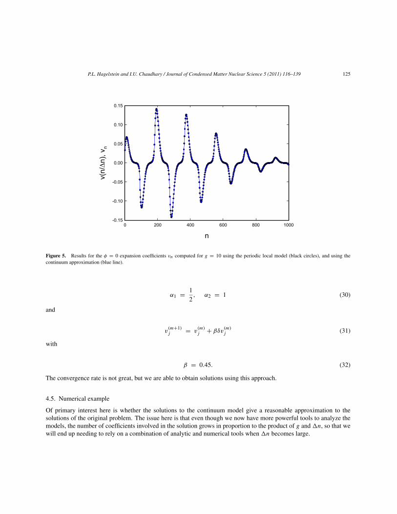
P.L. Hagelstein and I.U. Chaudhary / Journal of Condensed Matter Nuclear Science 5 (2011) 116–139 125
n0 200 400 600 800 1000
v(n/∆ n
), v n
-0.15
-0.10
-0.05
0.00
0.05
0.10
0.15
Figure 5. Results for the φ = 0 expansion coefficients vn computed for g = 10 using the periodic local model (black circles), and using thecontinuum approximation (blue line).
α1 = 1
2, α2 = 1 (30)
and
v(m+1)j = v
(m)j + βδv
(m)j (31)
with
β = 0.45. (32)
The convergence rate is not great, but we are able to obtain solutions using this approach.
4.5. Numerical example
Of primary interest here is whether the solutions to the continuum model give a reasonable approximation to thesolutions of the original problem. The issue here is that even though we now have more powerful tools to analyze themodels, the number of coefficients involved in the solution grows in proportion to the product of g and n, so that wewill end up needing to rely on a combination of analytic and numerical tools when n becomes large.

126 P.L. Hagelstein and I.U. Chaudhary / Journal of Condensed Matter Nuclear Science 5 (2011) 116–139
g/∆n2
0.0001 0.001 0.01 0.1
∆ n2 V
eff/4
g∆E
10-7
10-6
10-5
10-4
10-3
10-2
10-1
100
Figure 6. Scaled level splitting for n = 91 expressed as a scaled indirect matrix element from the periodic local model (blue line), and from thecontinuum approximation (red line).
In Fig. 5, we show the result from the continuum model (blue line) compared with the exact numerical coefficientsfrom the periodic local model (black circles). The agreement is good, although there is a small offset associated withthe continuum solution. The self-energy for the “exact” local periodic solution is
E(0) = − 34.4370 E. (33)
The result from 3-pt differencing of the continuum approximation with 91 points is
E(0) = − 34.4312 E (3 − pt discretization). (34)
We can correct this self-energy by including the contribution of the lowest-order discretization error to obtain
E(0) = − 34.4316 E (corrected 3 − pt discretization). (35)
We conclude that the continuum model itself as an approximation is responsible for most of the energy difference.The level splitting from the continuum model is shown in red in Fig. 6, compared with the periodic model result
in blue. We see that the continuum model result is very close to the periodic model result. We conclude from thesecalculations that we should be able to make use of the continuum model for self-energy and for level splitting calculationsand get good results.

P.L. Hagelstein and I.U. Chaudhary / Journal of Condensed Matter Nuclear Science 5 (2011) 116–139 127
5. Strong-coupling Limit
Direct numerical computations with the models described above becomes increasingly slow for larger values of g. Thisis because the solutions that make up the expansion coefficients include a large number of peaks, which involves alarge number of points. An additional difficulty is that the iterative algorithm discussed converges more slowly as morepoints are used. It is possible to make use of the models outlined above to obtain systematic results for large g, bytaking advantage of the presence of a large number of peaks. Since the peaks have nearly the same shape from onecycle to the next it becomes possible to develop strong coupling approximations.
5.1. Large g approximation for the periodic model
We see in Fig. 5 that the φ = 0 solutions are made up of peaks that alternate in sign, and that for large g we mightexpect that the peak amplitudes will become uniform. In this case we would write
vn+n = − vn (φ = 0). (36)
The eigenvalue equation for the expansion coefficients in this limit reduces to
ε0vn = n
nvn − 2g(vn+1 + vn−1). (37)
In the case of φ = π , the different peaks have the same sign, so that we would expect
vn+n = vn (φ = π). (38)
The corresponding eigenvalue equation in this large g limit is essentially the same
επvn = n
nvn − 2g(vn+1 + vn−1). (39)
We show the result of computations for n = 91 for the level splitting as a function of g in Fig. 7 for this strongcoupling approximation (red) compared with exact numerical results from the periodic model (blue). We see that thestrong coupling approximation approaches the exact solution at large g, and that it deviates some at low g. This isconsistent with our expectations, since when g is small only a few peaks make up the solution, in which case theassumption that the peaks are uniform (or linear) becomes poor.
5.2. Large g version of the continuum approximation
We can make a similar approximation in the case of the continuum approximation in the large g limit where there aremany peaks, and where the shapes and amplitudes are similar in the different peaks. The resulting large g approximationis
εv(z) = zv(z)− 4gv(z)− 2g
n2
d2v
dz2 (40)
for both φ = 0 and φ = π .This strong coupling continuum approximation is interesting because it predicts that the level splitting depends on
the ratio g/n2, but not on g independently. We can see this be recasting the eigenvalue equation as

128 P.L. Hagelstein and I.U. Chaudhary / Journal of Condensed Matter Nuclear Science 5 (2011) 116–139
g/∆n2
0.0001 0.001 0.01 0.1
∆ n2 V e
ff/4g∆
E
10-7
10-6
10-5
10-4
10-3
10-2
10-1
100
Figure 7. Scaled level splitting for n = 91 expressed as a scaled indirect matrix element from the periodic local model (blue line), and from thestrong coupling approximation (red line).
ε′v(z) = zv(z)− 2g
n2
d2v
dz2 , (41)
where
ε′ = ε + 4g. (42)
We noticed in our calculations that the discrete strong coupling approximation above gave very nearly the same levelsplittings as a function of g/n2 for different large values of n. We see now that such behavior is expected, sincewhen g is very large, it is only g/n2 that matters in determining the level splitting.
The calculated level splitting in this model is very close to the large g approximation result in Fig. 7.
5.3. Scaling law for indirect coupling matrix element
From the strong coupling results, we see that the indirect coupling matrix element obeys a scaling law of the form
Veff
E= 4
g
n2( g
n2
). (43)
For ease of use, we have fit the function (x) according to

P.L. Hagelstein and I.U. Chaudhary / Journal of Condensed Matter Nuclear Science 5 (2011) 116–139 129
(x) = expa + b ln x + c(ln x)2 + d(ln x)3 + e(ln x)4
(44)
using data in the range
0.00020 < x < 0.12. (45)
The fitting parameters that result are
a = − 1.11722, b = − 1.61939, c = − 0.780116, d = − 0.171302, e = − 0.0159906. (46)
5.4. Analytic model for the large g continuum model
We can solve the differential equation for the strong coupling continuum model using a solution of the form
v(z) = Ai
[(n2
2g
)1/3
(z− z0)
], (47)
ε = − 4g + z0, (48)
where Ai is an Airy function. A scaled version of this analytic result is shown in Fig. 8 compared with results fromexact numerical calculations with the local periodic model. We see that the agreement over most of the cycle is verygood. Deviations between the analytic solution and the exact solution on the small n side are due to the fact that thecoefficients at n−n are zero in the exact model (the analytic model here does not know about the cut-off at n = 0).
5.5. Peak amplitudes
If we assume that the different peaks have approximately the same shape, then it is possible to develop a model for thepeak amplitudes. To proceed, we assume that the expansion coefficients for the φ = 0 case can be approximated by
vn =∑m
(−1)mamun−mn, (49)
where am is the amplitude, and where un describes a single peak. For φ = 0, the eigenvalue equation is
ε0vn = n
nvn + g
[(vn+n+1 + vn+n−1)+ (vn−n+1 + vn−n−1)
], (50)
we can develop an equation for the amplitudes of the form
ε0〈un|un〉am = 〈un| nn
|un〉 − g〈un|un+1〉am+1 − g〈un|un−1〉am+1
−g〈un|un+1〉am−1 − g〈un|un−1〉am−1, (51)

130 P.L. Hagelstein and I.U. Chaudhary / Journal of Condensed Matter Nuclear Science 5 (2011) 116–139
n120 140 160 180 200 220 240
v n
0.00
0.01
0.02
0.03
0.04
0.05
0.06
Figure 8. Expansion coefficients for g = 30 and n = 151; φ = 0 (blue triangles); φ = π (red circles); and Airy function analytic model (blackline).
When g is large we may approximate
〈un|un+1〉〈un|un〉 → 1. (52)
We require an estimate the expectation value 〈n/n〉. Since each successive peak occurs at a position n unitspast the previous one, we would expect that the expectation value would be equal to m plus an offset that depends onthe width (which depends on g/n2). From the results of numerical calculations, the following approximation seemsreasonable
⟨ nn
⟩= m+ δn
( g
n2
). (53)
We can then reduce the amplitude equation to
[ε0 − δn
( g
n2
)]am = mam − 2g(am−1 + am+1). (54)
This equation can be solved analytically using a solution of the form
am = Jm+m0(4g), (55)

P.L. Hagelstein and I.U. Chaudhary / Journal of Condensed Matter Nuclear Science 5 (2011) 116–139 131
n0 500 1000 1500 2000 2500
v n
0.00
0.02
0.04
0.06
0.08
0.10
Figure 9. Expansion coefficients for g = 30, n = 151, and φ = π (blue); and results from the peak amplitude model (red).
where m0 is chosen so that the first zero of the Bessel function is matched to the boundary condition near n = 0. Weillustrate in Fig. 9 an example where we have chosen the φ = π version of the problem (in which the peaks all havethe same sign, so that it is easier to compare). In this case, we have used n = 151 and g = 30, and we have scaledthe amplitudes to approximately match the peak amplitude. We see that this model for the amplitudes is in reasonableagreement with the exact numerical calculation.
5.6. Continuum approximation for the peak amplitudes
When g becomes large there occur a great many peaks. In this case, we can adopt a continuum approximation
am → a(m) (56)
with
am+1 → a(m)+ da
dm+ 1
2
d2a
dm2 (57)
am−1 → a(m)− da
dm+ 1
2
d2a
dm2 . (58)
The eigenvalue equation becomes

132 P.L. Hagelstein and I.U. Chaudhary / Journal of Condensed Matter Nuclear Science 5 (2011) 116–139
[ε0 + 4g − δn
( g
n2
)]a(m) = ma(m)− 2g
d2a
dm2 . (59)
This is solved using
a(m) = Ai
[(1
2g
)1/3
(m− δm)
]. (60)
Here δm is chosen to match the boundary condition.
6. Dynamics for Strong Coupling
Since the indirect coupling matrix element obeys a scaling law in the strong coupling limit, it is possible to examinecoherent energy exchange under conditions where a large number of oscillator quanta are converted. From previouswork the dynamics is governed by
d2
dt2m = 2
h2
d
dmV 2(m). (61)
We assume in writing this that there are enough two-level systems present so that the nearly-degenerate set of indirectlycoupled states can be treated as degenerate. To proceed, we recall that
g = V√n√S2 −m2
E. (62)
In what follows we will simplify things by assuming that n does contribute to the dynamics. This would be the case ifa large n were imposed such that the energy exchange gives rise to only a small change in oscillator excitation. Thislimit might also be of interest if conventional oscillator loss limited the maximum excitation of the oscillator.
6.1. Scaled Dicke number
In what follows, it will be convenient to work with a scaled version of m; hence, we define y according to
y = m
S. (63)
The equation of motion can then be written as
d2
dt2y(t) = 2
h2S2
d
dy
[4E
g
n2( g
n2
)]2. (64)
We can simplify the subsequent algebra if we introduce gmax which we define as
gmax = V√nS
E. (65)

P.L. Hagelstein and I.U. Chaudhary / Journal of Condensed Matter Nuclear Science 5 (2011) 116–139 133
This allows us to write
d2
dt2y(t) = 32
S2
(E
h
)2 d
dy
[(gmax
n2
)2(1 − y2)2
(gmax
n2
√1 − y2
)]. (66)
6.2. Characteristic frequency
The scaling law here involves y appearing in the same way in the different terms. We can extract the physical parametersby introducing the scaled variable
ξ = gmax
n2
√1 − y2. (67)
This allows us to write
d2
dt2y(t) = 32
S2
(E
h
)2 d
dy
[ξ22 (ξ)
]= 32
S2
(E
h
)2 dξ
dy
d
dξ
[ξ22 (ξ)
]. (68)
We can evaluate the derivative in y to obtain
dξ
dy= − gmax
n2
y√1 − y2
. (69)
This leads to
d2
dt2y(t) = − 32
S2
(E
h
)2 (gmax
n2
)2y
(1
ξ
d
dξ
[ξ22 (ξ)
]). (70)
We can define a characteristic frequency 0 for this model to satisfy
20 = 1
S2
(E
h
)2 (gmax
n2
)2. (71)
This can be recast as
20 = 1
n4
(V
√n
h
)2
. (72)
The characteristic frequency 0 can then be written in the two equivalent forms
0 = 1
S
(E
h
)(gmax
n2
)= 1
n2
(V
√n
h
). (73)

134 P.L. Hagelstein and I.U. Chaudhary / Journal of Condensed Matter Nuclear Science 5 (2011) 116–139
ξ
10-3 10-2 10-1
F(ξ )
10-8
10-7
10-6
10-5
10-4
10-3
10-2
10-1
100
101
102
103
Figure 10. Function F(ξ) discussed in the text plotted as a function of ξ .
6.3. Nonlinearity
Ultimately we end up with the dynamics of a nonlinear oscillator which can be expressed as
d2
dt2y(t) = −2
0y
(32
ξ
d
dξ
[ξ22 (ξ)
]). (74)
To compute the dynamics of this system, it is convenient to define
F(ξ) = 32
ξ
d
dξ
[ξ22 (ξ)
]. (75)
We have evaluated this function (see Fig. 10 ), and fit it to the form
F(ξ) = exp
a + b ln ξ + c(ln ξ)2 + d(ln ξ)3 + e(ln ξ)4
(76)
with
a = 2.46013, b = − 3.22909, c = − 1.60184, d = − 0.362187, e = − 0.0332753. (77)

P.L. Hagelstein and I.U. Chaudhary / Journal of Condensed Matter Nuclear Science 5 (2011) 116–139 135
Γ0t
-10 -5 0 5 10
y(t)
-1.0
-0.5
0.0
0.5
1.0
Figure 11. Non-periodic solutions for y(t) as a function of scaled time for gmax/n2 values of 0.0003 (green), 0.001, 0.003, 0.01 (red). The time
scaling uses τ−1 = |y′(0)|.
6.4. Solutions
Using this function we may write for the evolution equation
d2
dt2y(t) = −2
0yF
(gmax
n2
√1 − y2
). (78)
In Fig. 11, we show non-periodic solutions that we computed for different values of gmax/n2. We scaled the time
axis of the different solutions by the maximum rate for the different cases in order to compare them. To do this, westart with the maximum reaction velocity
∣∣∣∣dm
dt
∣∣∣∣max
= 2
hmaxVeff = 8
(E
h
)(gmax
n2
)(gmax
n2
). (79)
The maximum rate for the normalized version of m can be written as
0 = 1
S
∣∣∣∣dm
dt
∣∣∣∣max
= 8
S
(E
h
)(gmax
n2
)(gmax
n2
)= √
20(gmax
n2
). (80)

136 P.L. Hagelstein and I.U. Chaudhary / Journal of Condensed Matter Nuclear Science 5 (2011) 116–139
6.5. Connection between the maximum rate and the coupling
One of the key questions that relates to these models concerns determining how large the coupling matrix element mustbe in order for coherent energy exchange to occur at a given rate. In the large n scaling that we have considered inthis section, we can determine the maximum reaction rate from the coupling matrix element by expressing0 in termsof V in the expression above to obtain
0 = √2
1
(n)2
V√n
h
(gmax
(n)2
). (81)
The coupling matrix element in this model is V√n, so it is natural to expect V
√n/h as providing the underlying
rate scale. The maximum rate is then smaller by a factor of (n)2, which is essentially the penalty in this model forfractionating the large two-level system quantum E into a large number of oscillator quanta with energy hω0. Thefunction is shown in Fig. 7, and we might regard this factor as an additional penalty factor required for insufficientlystrong coupling. Finally, we need to arrange for gmax/(n)
2 to be sufficiently large so that our penalty is not too great,which we can interpret as a constraint on the number of two-level systems required to fractionate the large quantum.
7. Discussion and Conclusions
The lossy spin-boson model is interesting in that it exhibits a strong coherent energy exchange effect between a setof two-level systems and an oscillator under conditions where the large energy quantum of the two-level systems isdivided into a large number of oscillator quanta. In previous papers, we have examined this using perturbation theory[10], and using a second-order formulation [12]. Our interest in the problem stems from seeking models for the excessheat effect in the Fleischmann–Pons experiment, where we interpret the experimental results as splitting a large nuclearquantum of energy into a very large number of atomic scale quanta associated with phonon modes of the lattice. Weare interested in this paper in the question of whether the lossy spin-boson model is capable coherent energy exchangeunder such conditions.
In a previous paper we introduced the periodic local approximation [13], which is a powerful tool which allows usto reduce a large and difficult two-dimensional (m and n) problem into a much smaller and easier one-dimensional (n)problem when a resonance condition is satisfied. In this paper we have exploited the local approximation to computeeigenfunctions, self-energies, and indirect coupling matrix elements for examples when the dimensionless couplingconstant is reasonably large and when many oscillator quanta are exchanged. After a number of such calculations, wehave found that the system appears to obey a scaling law for the self-energy, and a scaling law for the indirect couplingmatrix element. The is interesting in its own right, since we had no reason a priori to expect such behavior. Alsointeresting is that the self-energy and indirect matrix elements show convergence to the strong coupling limit result ina regime where we can perform calculations directly, enabling us to verify the behavior of the system independently.
With the aid of the scaling law for the indirect coupling matrix element, we are able to carry out computations ofthe resulting system dynamics in the strong coupling regime where coherent energy exchange occurs with a very largenumber of oscillator quanta. In the end, we see that this lossy spin-boson model is able to exchange energy efficientlyeven when the two-level system transition energy is very much less than the characteristic energy of the oscillator. Forthis to work, the system must be in a very strong coupling regime, which can be done by simply increasing the numberof two-level systems. The price to be paid for such a large mismatch is a reduction in the coherent energy transferrate. In the large n model, the rate 0 scales as (n)−2 when n is increased and gmax/n
2 is held fixed. Suchscaling is relatively gentle, which encourages us in exploring it for application to excess heat in the Fleischmann–Ponsexperiment. The coherent energy transfer rate in the finite n model discussed in the Appendix is much faster.

P.L. Hagelstein and I.U. Chaudhary / Journal of Condensed Matter Nuclear Science 5 (2011) 116–139 137
In looking forward, much work remains to develop a usable theory for the Fleischmann–Pons experiment. We willneed to generalize the model to describe donor and receiver two-level (as well as n-level) systems. Our computations inthis paper were carried out in an infinite loss approximation, and we will need to develop models with finite oscillatorloss at E in order to connect with experiment. In our computations in the strong coupling limit in this work, acharacteristic feature of the solutions is that a very large number of different oscillator n-states are occupied when g islarge. In the physical system the oscillator sees loss at ω0, so that one would expect the results to depend on this loss.We would like to examine models which shed light on this. We will also need to connect this simple two-level systemand oscillator models to the physical system, which will require a derivation of the model as well as an evaluation ofthe coupling matrix elements.
Appendix A. A Finite n Model
We chose the simple model discussed in the previous subsections in part because it was simple and informative.However, the restriction that the number of oscillator quanta is not changed by the dynamics is a strong one, and weare interested here in the generalization to the case where the change in the number of oscillator quanta is significant.
Appendix A.1. Energy conservation
In this case, the number of oscillator quanta n would depend explicitly onm. If we assume that the oscillator loss at ω0can be neglected, then we may use energy conservation to write
n0 = n+n(S +m). (A.1)
In this model the number of oscillator quanta decreases when the number of excited two-level systems increases.
Appendix A.2. Evolution equation
The relation between the local g and m is modified to read
g = V√n0 −n(S +m)
√S2 −m2
E. (A.2)
We use this to generalized the definition of ξ to
ξ = g
n2 = V S√n0 −nS(1 + y)
√1 − y2
En2 . (A.3)
We then compute
dξ
dy= − g
n2
[y
1 − y2 + Sn
2n
], (A.4)
where we note that g and n both depend on y.The evolution equation in general can be written as
d2
dt2y(t) = 32
S2
(E
h
)2 dξ
dy
d
dξ
[ξ22 (ξ)
]. (A.5)

138 P.L. Hagelstein and I.U. Chaudhary / Journal of Condensed Matter Nuclear Science 5 (2011) 116–139
Using the expression above for the derivative dξ/dy, we obtain
d2
dt2y(t) = − V 2n
h2n4
[y + Sn
2n(1 − y2)
]F(ξ). (A.6)
Note that n and ξ depend explicitly on y in this evolution equation.
Appendix A.3. Steady-state condition
If all of the two-level systems are initialized in the ground state, and if the oscillator is initialized in an excited state,we would expect that some of the two-level systems would become excited. We can determine how many are excitedin the steady state by solving
y + Sn
2n(1 − y2) = 0. (A.7)
We use
n = n0 −nS(1 + y) (A.8)
to obtain the constraint
3y2 + 2(
1 − n0
nS
)− 1 = 0. (A.9)
We assume that the amount of excitation is small, and obtain the approximate result
y = − 1 + n0
2nS. (A.10)
The number of excited two-level systems in this case is
m+ S = 1
2
n0
n= n
n. (A.11)
This is the condition at which the contributions that increase the indirect matrix elements are the same for the two-levelsystems as for the oscillator.
Appendix A.4. Discussion
In the large n model described in Section 6, if the oscillator is initially excited and the two-level systems are in theground state, then the model predicts that in time all of the two-level systems would be excited. One of the reasons forgoing to a finite n model is that now the matrix elements increase when the number of oscillator quanta increases, sothat the two-level systems in such a model want to give up their energy to the oscillator. In this new model, the rate atwhich the two-level systems give up their energy is increased by roughly Sn/n over that of the large n limit, a factorwhich can be very large.
If the two-level systems are initially in the ground state, then we would expect that they can be excited if theoscillator is highly excited. The evolution equation for this model gives this result. The large n model and this energy

P.L. Hagelstein and I.U. Chaudhary / Journal of Condensed Matter Nuclear Science 5 (2011) 116–139 139
conserving finite n model exhibit two different limits for coherent energy exchange. Unfortunately, there are issueswith both models in connection with modeling excess heat in the Fleischmann—Pons experiment. If we are interestedin coupling energy to optical phonon modes, it can never be the case that the system can reach a large n limit, becausethe associated thermal power would be so high as to be physically unreasonable (since the thermalization time of thesephonon modes is so short). Since optical phonon modes are so lossy, a model which enforces energy conservationwithout optical phonon loss also seems not so realistic. To do better, we will need to include phonon loss.
References
[1] M. Fleischmann, S. Pons and M. Hawkins, J. Electroanal Chem. 201 (1989) 301; errata, 263 (1990) 187.[2] M. Fleischmann, S. Pons, M.W. Anderson, L.J. Li and M. Hawkins, J. Electroanal. Chem. 287 (1990) 293.[3] M.H. Miles, R.A. Hollins, B.F. Bush, J.J. Lagowski and R.E. Miles, J. Electroanal. Chem. 346 (1993) 99.[4] M.H. Miles, B.F. Bush and J.J. Lagowski, Fusion Technol. 25 (1994) 478.[5] M.H. Miles, Correlation of excess enthalpy and helium-4 production: A review, Proc. ICCF10, 2004, p. 123.[6] P.L. Hagelstein, M.C.H. McKubre, D.J. Nagel, T.A. Chubb and R.J. Hekman, New physical effects in metal deuterides, Proc.
ICCF11, 2005, p. 23.[7] P.L. Hagelstein, Naturwissenschaften 97 (2010) 345.[8] D. Letts, D. Cravens and P.L. Hagelstein, Dual laser stimulation and optical phonons in palladium deuteride, in low-energy
nuclear reactions and new energy technologies, Low-Energy Nuclear Reactions Sourcebook, Vol. 2, American Chemical Society,Washington, DC, 2009, p. 81.
[9] P.L. Hagelstein, D. Letts and D. Cravens, Terahertz difference frequency response of PdD in two-laser experiments, J. Cond.Mat. Nucl. Sci. 3 (2010) 59.
[10] P.L. Hagelstein and I.U. Chaudhary, Energy exchange in the lossy spin-boson model, J. Cond. Mat. Nucl. Sci. 5 (2011) 52.[11] P.L. Hagelstein and I.U. Chaudhary, Dynamics in the case of coupled degenerate states, J. Cond. Mat. Nucl. Sci. 5 (2011) 72.[12] P.L. Hagelstein and I.U. Chaudhary, Second-order formulation and scaling in the lossy spin-boson model, J. Cond. Mat. Nucl.
Sci. 5 (2011) 87.[13] P.L. Hagelstein and I.U. Chaudhary, Local approximation for the lossy spin-boson model, J. Cond. Mat. Nucl. Sci. 5 (2011)
102.

J. Condensed Matter Nucl. Sci. 5 (2011) 140–154
Research Article
Generalization of the Lossy Spin–Boson Model to Donor andReceiver Systems
Peter L. Hagelstein ∗Research Laboratory of Electronics, Massachusetts Institute of Technology, Cambridge, MA 02139, USA
Irfan U. ChaudharyDepartment of Computer Science and Engineering, University of Engineering and Technology. Lahore, Pakistan
Abstract
Energy in the Fleischmann–Pons experiment is produced without commensurate energetic particles, and 4He is seen in amountsproportional to the energy produced (with a ratio of energy to number near 24 MeV). Correspondingly we focus on the D2/ 4Hetransition as a two-level system coupled to an oscillator, in order to make a connection with the lossy spin–boson model consideredin previous work. Because of the strong Coulomb repulsion between the deuterons, the associated coupling matrix element is verysmall, and there is no possibility of converting the transition energy to oscillator quanta within a simple lossy spin–boson model. Thismotivates us to generalize to more complicated model that includes a set of (donor) two-level systems for the D2/ 4He transition, anda set of (receiver) two-level systems that are strongly coupled to the oscillator. We analyze the resulting model in the limit that thereceiver system is very strongly coupled. Within this formulation, the associated dynamics can be interpreted in terms of a transitionfrom D2 to 4He with direct conversion (and fractionation) of the large energy quantum to the oscillator, once the coupling with thereceiver system is sufficiently strong.© 2011 ISCMNS. All rights reserved.
Keywords: Coherent Fusion, Donor–receiver Model, Excitation Transfer, Theory Excess Heat in the Fleischmann–Pons Experiment
1. Introduction
In the previous papers, we introduced the lossy spin–boson model, and we studied the ability of the model to describethe fractionation of a large quantum [1–5]. Our goal in these studies has been to develop new models relevant to excessheat production in the Fleischmann–Pons experiment [6], where a large amount of energy is made [7], 4He is observed
∗E-mail: [email protected]
© 2011 ISCMNS. All rights reserved.

P.L. Hagelstein and I.U. Chaudhary / Journal of Condensed Matter Nuclear Science 5 (2011) 140–154 141
in amounts commensurate with the energy produced [8,9], and where no commensurate energetic particles are observed[10].
The fundamental question that was the focus of our earlier work is whether a large nuclear-scale quanta can befractionated into a large number of much smaller quanta relevant to condensed matter degrees of freedom. Our approachin this study was to focus on equivalent two-level systems and an oscillator, in an effort to simplify the problem asmuch as possible (since the associated models and coherent dynamics are much more complicated than for incoherentreactions). As a result, it was not important to specify precisely which levels were involved. Had our ultimate conclusionbeen otherwise (that fractionating a large quantum was impossible), then there would have been no need to examinespecific cases.
1.1. General mathematical models versus specific physical models
Our results suggest that a large quantum can be fractionated, and we have explicit models which show the effect andwhich we can analyze quantitatively. This now opens the door to trying to connect the general model to specificexamples of models of this type for evaluation. This new problem that we face now must be viewed as a significantproblem in its own right. One new task is to identify upper and lower levels of the two-level systems with specificnuclear states, and another is to associate specific condensed matter oscillatory modes to the harmonic oscillator in themodel.
Ideally, we would like for experiment to provide an unambiguous positive identification for us the states that areinvolved, and to make perfectly clear which oscillator is relevant. Unfortunately, in the experiments that have been doneso far, and we generally lack the experimental clarity that would result in unambiguous choices. Consequently, there isnot agreement within the community of scientist working on the problem as to what states should be focused on, and atthis point some discussion of the problem is worth while. In the remainder of this Introduction, we summarize brieflysome of the discussion that has occurred within our group over the years.
1.2. Lossy spin–boson model for the D2 to 4He transition
If we select molecular D2 (keeping in mind that there are a number of such states) for the upper state of the two-levelsystem, and 4He for the lower state, then the resulting model would predict a ratio of excess energy to the number of4He atoms to be 23.85 MeV, which is consistent with the two experiments that measure the ratio under conditions wherean attempt was made to recover the helium retained in the cathode [11,12].
Unfortunately, the associated coupling matrix element is exceedingly small because of Coulomb repulsion. If wemodel the system using a lossy spin–boson model, then we quickly conclude that it is impossible to fractionate thelarge quantum with these states alone since the associated coupling matrix element is so small.
1.3. Generalization of the model and excitation transfer
Because of this, we decided (many years ago) to generalize the model in order to have a more complicated system inwhich the D2/ 4He transition would supply the large energy quantum, and another transition would be involved in thefractionation of the quantum.
For this to work, we require a new fundamental mechanism that takes the energy associated with a transition at onesite, and transfers it to another site. There is precedence for such a physical effect in biophysics, in which an excitedmolecule is observed to transfer its excitation (through a Coulomb interaction) to another molecule. In this case, theeffect is termed “resonance energy transfer”, or “Förster effect” (in honor of the physicist who first gave a quantitativemodel for the effect [13,14]). There is no reason to believe that a nuclear version of the Förster effect should not be

142 P.L. Hagelstein and I.U. Chaudhary / Journal of Condensed Matter Nuclear Science 5 (2011) 140–154
able to exist for nuclei, but from calculation we know that a version of the effect that depends on Coulomb interactionsalone cannot do what we require (because the Coulomb dipole–dipole interaction is of short range).
For us, the solution to this problem was to focus on phonon exchange instead of Coulomb exchange, since we foundthat a much longer range for the effect could work in the case of phonon exchange with a highly excited phonon mode.This is very closely connected with the kinds of models we discussed earlier. For example, one can establish the effectusing perturbation theory in a model with two different two-level systems each coupled linearly to an oscillator. Asa result, this new excitation transfer mechanism comes into the problem in a natural way in the generalization of ourmodel from one set of two-level systems to two sets of two-level systems, both coupled to a common oscillator.
1.4. But what transition would fractionate the large quantum?
From the beginning of our research on this generalization, we have faced the issue of specifying a second set of two-levelsystems which would fractionate the large quantum, and convert the energy to a condensed matter mode. Models withdifferent choices have been studied, and from these studies we have begun to understand what the relevant issues are.
In the early days of our work, we thought that the most important issue in the selection of the second set of two-levelsystems was the degree of resonance with the D2/ 4He transition energy. As a result, it seemed natural to considertransitions between 4He as the ground state, and whatever two-deuteron states were available near the initial transitionenergy (23.85 MeV), since we would come closest to obtaining a resonance.
Once we began to understand phonon exchange in association with nuclear transitions better, and when we alsounderstood the coherent models better, it became clear that the Pd isotopes should be considered as candidates. Arguingfor this approach is that Pd is the primary constituent of the host lattice, so that we might expect it to be numericallydominant.
We focused at one point on transitions to excited states, composed of a neutral plus daughter, that seemed to befavored in exchanging phonons; one such example was the 110Pd/106Pd+4n transition. This transition is probably notsuch a close match in energy to the D2/ 4He transition, so the issue of energy exchange in connection with excitationtransfer becomes important.
Recently, we undertook a systematic effort to see whether we could identify candidate transitions that would be ableto serve as receivers in the donor-receiver model under discussion in this work. The general approach that we used wasto derive constraints directly from our model, and we examined several hundred nuclear and atomic transitions to seehow closely the constraints could be satisfied. It quickly came clear from this analysis that no physical transition canstand in for the receiver-side of this model, since we ask for too much. Perhaps the biggest issue in this study is thatwe require a large coupling matrix from the ground state, and also a long lifetime so that coherence can be preserved;yet generally a large coupling matrix element implies a short radiative lifetime.
Because of this, we have adopted a revised point of view concerning this simple donor-receiver model, with twosets of two-level systems coupled to an oscillator, and augmented with loss. Certainly it is the simplest model thatdemonstrates the basic physical effects we require: the ability to exhange energy coherently under conditions wherea large quantum is fractionated, and the ability to transfer excitation from one two-level system to another. But sincethe receiver system doesn’t correspond to a simple physical transition, we view it as a likely idealization of a morecomplicated receiver system that involves three or more levels. But the two-level systems of the donor side of the modelappears relevant to the D2/ 4He transition, allowing us to study the donor dynamics in the presence of an idealizedreceiver system.
1.5. But what about the oscillator?
The oscillator in the general two-level system and oscillator models can in principle represent any condensed matteroscillatory mode, and the question at issue is what modes are involved. The candidates in principle include acoustic

P.L. Hagelstein and I.U. Chaudhary / Journal of Condensed Matter Nuclear Science 5 (2011) 140–154 143
phonon modes, optical phonon modes (with compressional modes at the-point and L-point apparently preferred in thetwo-laser experiment), and plasmon modes (which we expect to be mixed with optical phonon modes, and which areimplicated in single laser experiments). There is no reason to exclude any of these modes in the basic Fleischmann–Ponsexperiment, based on measurements done so far. In the single laser experiment, probably a plasmon mode is involved.In the two-laser experiment [15,16] specific optical phonon modes are involved. In what follows our focus will be onoptical phonon modes, primarily since the resulting model seems “cleanest” to us (optical phonon modes couple wellwith the D2/ 4He transition).
2. Generalization of the Lossy Spin–Boson Model
Based on the above discussion, we generalize the lossy spin–boson model to include two different sets of two-levelsystems
H = E1S(1)z
h+E2
S(2)z
h+ hω0a
†a + V1e−G(a† + a)2S(1)xh
+ V2(a† + a)
2S(2)xh
− ih
2(E). (1)
The first set of two-level systems will have transition energy E1, and will be considered to be the “donor” systemwithin the model (in the sense that excitation is transferred from this system); the second set of two-level systems (the“receiver” system) in general has a different transition energyE2. The oscillator has a characteristic energy hω0. Weinclude linear coupling terms between the oscillator and each of the two sets of two-level systems, with the couplingconstant V1e−G for coupling from the first set of two-level systems (where e−G accounts for transitions from the firstset of two-level systems being hindered by the tunneling factor associated with tunneling through the Coulomb barrier),and V2 for coupling with the second set of two-level systems. Loss is included through a Brillouin–Wigner type of lossoperator as we have discussed previously.
3. Local Approximation for the Generalized Lossy Spin–Boson Model
We are interested ultimately in a regime in which the coupling between the receiver system and the oscillator is verystrong. In our previous work on coherent energy exchange, we found that the system could be understood by takingadvantage of the local approximation, since direct calculations when the coupling is very strong are computationallyexpensive. For the generalized lossy spin–boson model we would like to make use of the local approximation for ouranalysis.
3.1. Eigenvalue equation for the expansion coefficients
To proceed, we begin with a finite basis expansion for this more complicated system in the form
=∑m1
∑m2
∑n
cm1,m2,n|S1,m1〉|S2,m2〉|n〉. (2)
For the wave function to satisfy the time-independent Schrödinger equation, the expansion coefficients cm1,m2,n
satisfy

144 P.L. Hagelstein and I.U. Chaudhary / Journal of Condensed Matter Nuclear Science 5 (2011) 140–154
Ecm1,m2,n =[E1m1 +E2m2 + hω0n− i
h
2(E)
]cm1,m2,n
+ V1e−G√n+ 1
√(S1 −m1)(S1 +m1 + 1)cm1+1,m2,n+1
+ V1e−G√n√(S1 −m1)(S1 +m1 + 1)cm1+1,m2,n−1
+ V1e−G√n+ 1
√(S1 +m1)(S1 −m1 + 1)cm1−1,m2,n+1
+ V1e−G√n√(S1 +m1)(S1 −m1 + 1)cm1−1,m2,n−1
+ V2√n+ 1
√(S2 −m2)(S2 +m2 + 1)cm1,m2+1,n+1
+ V2√n√(S2 −m2)(S2 +m2 + 1)cm1,m2+1,n−1
+ V2√n+ 1
√(S2 +m2)(S2 −m2 + 1)cm1,m2−1,n+1
+ V2√n√(S2 +m2)(S2 −m2 + 1)cm1,m2−1,n−1. (3)
3.2. Limit of many oscillator quanta and two-level systems
Previously we used large n and large S approximations to develop a local approximation. Here we need to do the same.We assume that n is large to write
√n+ 1 ≈ √
n. (4)
For the different two-level systems, we make the approximation
√(Sj −mj)(Sj +mj + 1) ≈
√S2j −m2
j , (5)
√(Sj +mj)(Sj −mj + 1) ≈
√S2j −m2
j . (6)
If each Sj is very large, and if each mj is not close to ±Sj , then these approximations should be good ones.
3.3. Local approximation
The coupling coefficients become the same to different states when we make this approximation, which leads directlyto a local approximation for this model
Ecm1,m2,n =[E1m1 +E2m2 + hω0n− i
h
2(E)
]cm1,m2,n
+ V1e−G√n
√S2
1 −m21 (cm1+1,m2,n+1 + cm1+1,m2,n−1 + cm1−1,m2,n+1 + cm1−1,m2,n−1)
+ V2√n
√S2
2 −m22 (cm1,m2+1,n+1 + cm1,m2+1,n−1 + cm1,m2−1,n+1 + cm1,m2−1,n−1). (7)
It is convenient to define two dimensionless coupling constants according to

P.L. Hagelstein and I.U. Chaudhary / Journal of Condensed Matter Nuclear Science 5 (2011) 140–154 145
g1 =V1
√n
√S2
1 −m21
E1, (8)
g2 =V2
√n
√S2
2 −m22
E2. (9)
We can rewrite the eigenvalue equation for the expansion coefficients as
Ecm1,m2,n =[E1m1 +E2m2 + hω0n− i
h
2(E)
]cm1,m2,n
+E1g1e−G (cm1+1,m2,n+1 + cm1+1,m2,n−1 + cm1−1,m2,n+1 + cm1−1,m2,n−1)
+E2g2 (cm1,m2+1,n+1 + cm1,m2+1,n−1 + cm1,m2−1,n+1 + cm1,m2−1,n−1). (10)
This is consistent with a local configuration space Hamiltonian of the form
H = E1m1 +E2m2 + hω0n− ih
2(E)
+E1g1e−G(δn+ + δn−)(δm1+ + δ
m1− )
+E2g2 (δn+ + δn−)(δ
m2+ + δm2− ). (11)
4. Periodic Donor and Receiver Models
In the strong coupling limit direct calculations of eigenfunctions, eigenvalues, and indirect coupling matrix elementsbecomes increasingly difficult the stronger the coupling. In the periodic model the problem simplifies, allowing us tomake use of numerical and analytic approaches. We use this approach here to analyze donor–receiver models underconditions where the coupling between the oscillator and the receiver two-level systems is very strong.
4.1. Periodic approximation and resonance condition
One of the most important tools that we have for analyzing coherent energy exchange in the strong coupling regime isthe periodic approximation. Since we would like to understand the generalized lossy spin–boson model when n isvery large for the receiver system, it seems reasonable to once again make use of the period version of the problem.Since there are two sets of two-level systems, we are going to require two distinct resonance conditions. For coherentenergy exchange between the receiver system and oscillator, we require
E2 = n2hω0. (12)
For excitation transfer transitions, we require
E1 = E2 +n12hω0. (13)

146 P.L. Hagelstein and I.U. Chaudhary / Journal of Condensed Matter Nuclear Science 5 (2011) 140–154
Even though we do not expect direct coherent energy exchange between the donor two-level systems and the oscillator,it is useful to define n1 to satisfy
E1 = n1hω0. (14)
4.2. Periodic solution
When the above resonance condition is satisfied, we can construct a locally periodic solution of the form
=∑m1
∑m2
∑n
dm1,m2un+m1n1+m2n2 |S1,m1〉|S2,m2〉|n+m1n1 +m2n2〉. (15)
It is possible to develop eigenfunction solutions for the local Hamiltonian using
dm1,m2 = ei(m1φ1+m2φ2). (16)
4.3. Eigenvalue equation
We assume that the wavefunction satisfies the time-independent Schrödinger equation, and then we use orthogonalityto obtain an eigenvalue equation for the expansion coefficients
Edm1,m2un+m1n1+m2n2
=[E1m1 +E2m2 + nhω0 − i
h
2(E)
]dm1,m2un+m1n1+m2n2
+ g1e−GE1[dm1+1,m2(un+1+(m1+1)n1+m2n2 + un−1+(m1+1)n1+m2n2)
+ dm−1,m2(un+1+(m1−1)n1+m2n2 + un−1+(m1−1)n1+m2n2)]+ g2E2[dm1,m2+1(un+1+m1n1+(m2+1)n2 + un−1+m1n1+(m2+1)n2)
+ dm1,m2−1(un+1+m1n1+(m2−1)n2 + un−1+m1n1+(m2−1)n2)]. (17)
If we make use of Eq. (16), then this can be simplified to
E(φ1, φ2)un =[nhω0 − i
h
2(E)
]un
+ g1e−GE1[eiφ1(un+1+n1 + un−1+n1)+ e−iφ1(un+1−n1 + un−1−n1)]+ g2E2[eiφ2(un+1+n2 + un−1+n2)+ e−iφ2(un+1−n2 + un−1−n2)], (18)
where we have focused as before on the special case of m1 and m2 equal to zero.
4.4. Solution for the second set of two-level systems
In this problem, the first set of two-level systems is weakly coupled to the oscillator, while the second set of two-levelsystems is strongly coupled. As a result, we would expect that the strong coupling associated with the second set of

P.L. Hagelstein and I.U. Chaudhary / Journal of Condensed Matter Nuclear Science 5 (2011) 140–154 147
two-level systems would dominate the problem. We have considered such a problem previously. It is possible to adaptit here by first taking
g1e−G → 0 (19)
and writing
E2(φ2)vn(φ2) =[nhω0 − i
h
2(E)
]vn(φ2)
+ g2E2[eiφ2(vn+1+n2(φ2)+ vn−1+n2(φ2))
+ e−iφ2(vn+1−n2(φ2)+ vn−1−n2(φ2))], (20)
where the vn(φ2) are the same coefficients that we studied previously in Ref. [5], and where E2(φ2) is the associatedenergy eigenvalue. We found previously that this energy eigenvalue in the strong coupling regime with large n2 isapproximately
E2(φ2) → 2(g2)+ 2V eff2 cosφ2, (21)
where 2 is the self-energy which we found previously in the strong coupling limit to be
2(g2) → − 4g2 (22)
and where V eff2 is [5]
V eff2 → 4g2
n22
E2
(g2
n22
). (23)
4.5. Perturbation theory estimate for the energy eigenvalue
We can use this as a starting point to estimate the energy eigenvalue. We can use perturbation theory to write
E(φ1, φ2) ≈ E2(φ2)+⟨vn(φ2)
∣∣∣∣g1e−GE1
[eiφ1
[vn+1+n1(φ2)+ vn−1+n1(φ2)
]
+e−iφ1[vn+1−n1(φ2)+ vn−1−n1(φ2)
]]⟩. (24)
We saw from earlier work that the expansion coefficients are slowly varying in the strong coupling limit, so that
vn+1−n1(φ2) ≈ vn−n1(φ2). (25)
Hence, we may write
E(φ1, φ2) ≈ E2(φ2)
+ 2g1e−GE1[eiφ1〈vn(φ2)|vn+n1(φ2)〉 + e−iφ1〈vn(φ2)|vn−n1(φ2)〉]. (26)

148 P.L. Hagelstein and I.U. Chaudhary / Journal of Condensed Matter Nuclear Science 5 (2011) 140–154
The bra and kets here denote summations over the different n, and we may write
〈vn(φ2)|vn+n1(φ2)〉 = 〈vn(φ2)|vn−n1(φ2)〉∗. (27)
Hence
E(φ1, φ2) ≈ E2(φ2)+ 4g1 e−GE1Reeiφ1〈vn(φ2)|vn+n1(φ2)〉. (28)
5. Dynamics of the Donor System
Our attention is first drawn to the dynamics of the donor system. Instead of dealing with the more complicated problemassociated with both the donor and receiver systems, we wish to first study the donor dynamics independently. Asidefrom the fact that it greatly simplifies the problem, this study will emphasize a key feature of how this coupled systemworks. We will see that under some conditions it becomes possible for the transition energy of the donor system to beconverted directly to the oscillator, as a result of the oscillator being strongly coupled with the other two-level system.
5.1. Dynamical equations for the expansion coefficients
We begin with a wave function definition of the form
=∑m1
∑m2
∑n
dm1(t)eim2φ2un+m1n1+m2n2 |S1,m1〉|S2,m2〉|n+m1n1 +m2n2〉. (29)
The associated evolution equation becomes
ihd
dtdm1(t)e
im2φ2un+m1n1+m2n2
=[E1m1 +E2m2 + nhω0 − i
h
2(E)
]dm1(t)e
im2un+m1n1+m2n2
+ g1e−GE1[dm1+1(t)eim2φ2(un+1+(m1+1)n1+m2n2 + un−1+(m1+1)n1+m2n2)
+ dm−1(t)eim2φ2(un+1+(m1−1)n1+m2n2 + un−1+(m1−1)n1+m2n2)]
+ g2E2[dm1(t)ei(m2+1)φ2(un+1+m1n1+(m2+1)n2 + un−1+m1n1+(m2+1)n2)
+ dm1(t)ei(m2−1)φ2(un+1+m1n1+(m2−1)n2 + un−1+m1n1+(m2−1)n2)]. (30)
We first simplify the phases to write

P.L. Hagelstein and I.U. Chaudhary / Journal of Condensed Matter Nuclear Science 5 (2011) 140–154 149
ihd
dtdm1(t)un+m1n1+m2n2
=[E1m1 +E2m2 + nhω0 − i
h
2(E)
]dm1(t)un+m1n1+m2n2
+ g1e−GE1[dm1+1(t)(un+1+(m1+1)n1+m2n2 + un−1+(m1+1)n1+m2n2)
+ dm−1(t)(un+1+(m1−1)n1+m2n2 + un−1+(m1−1)n1+m2n2)]+ g2E2[eiφ2(un+1+m1n1+(m2+1)n2 + un−1+m1n1+(m2+1)n2)
+ e−iφ2(un+1+m1n1+(m2−1)n2 + un−1+m1n1+(m2−1)n2)]dm1(t). (31)
We then approximate
un → vn(φ2) (32)
and obtain
ihd
dtdm1(t) ≈ E2(φ2)dm1(t)
+ 2g1e−GE1[dm1+1(t)〈vn+m1n1+m2n2 |vn+(m1+1)n1+m2n2〉+ dm−1(t)〈vn+m1n1+m2n2 |vn+(m1−1)n1+m2n2〉], (33)
where we have used a reference energy offset based on m1 = 0 and m2 = 0. This can be denoted more simply as
ihd
dtdm1(t) ≈ E2(φ2)dm1(t)
+ 2g1e−GE1[dm1+1(t)〈vn(φ2)|vn+n1(φ2)〉 + dm−1(t)〈vn(φ2)|vn−n1(φ2)〉]. (34)
5.2. Interpretation
In the solution that we adopted, the basis states are presumed degenerate as an ansatz of the model. As a result,we expected to obtain evolution equations with indirect coupling between distant expansion coefficient of degeneratestates (distant in n, but nearest neighbors in m1), and this corresponds to our result of Eq. (34). However, this resultdeserves some consideration in its own right in terms of the associated physical mechanism that has come out of themodel we proposed. In previous work we considered models in which the donor system would transfer excitation tothe receiver system, and then the receiver system would convert it to oscillator energy.
However, what we have found using this formulation in the strong coupling limit is qualitatively different, and muchsimpler. In essence, once there is sufficient coupling between the oscillator and receiver system, then the oscillator statesbecome spread, allowing the donor transition energy to be accepted directly by the oscillator. This differs qualitativefrom our earlier proposals and models.
The overlap integral 〈vn(φ2)|vn+n1(φ2)〉 is a function of the dimensionless coupling of the receiver system g2, eventhough we have not denoted this dependence explicitly. When the coupling between the receiver system and oscillatoris too weak, then the overlap integral becomes vanishingly small. When the coupling is strong, and the donor transitionenergy is approximately matched to a multiple of the receiver system transition energy, then the overlap approachesunity.

150 P.L. Hagelstein and I.U. Chaudhary / Journal of Condensed Matter Nuclear Science 5 (2011) 140–154
5.3. Evolution equations for expectation values
We may write for the evolution equation for the expansion coefficients an equivalent dynamical equation of the form
ihd
dtdm1 = Vm1+ 1
2dm1+1 + Vm1− 1
2dm1−1, (35)
where we have discarded the unimportant constant energy offset. In the event that φ2 is 0 or π , then the couplingcoefficients are real; otherwise they can be complex. In such cases we may write
Vm1+ 12
= |Vm1+ 12|eiθ , (36)
Vm1− 12
= |Vm1− 12|e−iθ . (37)
If we define scaled expansion coefficients according to
em1 = dm1eim1θ (38)
then the associated evolution equation is
ihd
dtem1 = |Vm1+ 1
2|em1+1 + |Vm1− 1
2|em1−1. (39)
We define the expectation value of the Dicke number m1 as
〈m1〉 =∑m1
m1|em1 |2. (40)
The associated evolution equations are
d
dt〈m1〉 = 〈v1〉, (41)
d
dt〈v1〉 = 2
h2
∑m1
|em1 |2(|Vm1+ 1
2|2 − |Vm1− 1
2|2). (42)
5.4. Classical limit
In the classical limit we may write
d2
dt2m1(t) = 2
h2
d
dm1[V eff
1 ]2 (43)
using

P.L. Hagelstein and I.U. Chaudhary / Journal of Condensed Matter Nuclear Science 5 (2011) 140–154 151
V eff1 = 2g1e−GE1|〈vn(φ2)|vn+n1(φ2)〉|. (44)
Most of the factors that make up the indirect coupling coefficient for the donor system V eff1 do not depend on m1; the
overlap matrix element depends on parameters associated with the receiver system, but not the donor system. As aresult, we may write
d2
dt2m1(t) = 2
h2 4e−2G(E1)2|〈vn(φ2)|vn+n1(φ2)〉|2 d
dm1g2
1
= 2
h2 4e−2GV 21 n|〈vn(φ2)|vn+n1(φ2)〉|2 d
dm1(S2
1 −m21)
= −[
16V 21 n
h2 e−2G|〈vn(φ2)|vn+n1(φ2)〉|2]m1(t). (45)
It may be most useful to write this as
d2
dt2m1(t) = − [1(g2, φ2)]2m1(t) (46)
with
1(g2, φ2) = 4
(V1
√n
he−G
)|〈vn(φ2)|vn+n1(φ2)〉|. (47)
The characteristic frequency associated with the donor system is seen to be four times the coupling matrix element(including the Gamow factor) divided by h, times a hindrance factor (magnitude of the overlap matrix element) thatdepends on the receiver system.
5.5. Analytic solution when the receiver system is static
In the event that we impose (mathematically) a condition of steady state on the receiver system, the associated dynamicsof the donor system will be oscillatory. As an example, if all of the two-level systems of the donor system are initiallyexcited, then the relevant classical solution is
m1(t) = S1 cos(1t). (48)
We see that the dynamics are determined by the characteristic frequency.
6. Discussion and Conclusions
Since the coupling is so weak in the case of the D2/ 4He transition, we have generalized the lossy spin–boson model tothe present donor-receiver model that includes two sets of two-level systems coupled to an oscillator. We recognize thismodel as an simplification of a more complicated model, as the two-level system of the receiver side is an idealizationof a system involving more levels.

152 P.L. Hagelstein and I.U. Chaudhary / Journal of Condensed Matter Nuclear Science 5 (2011) 140–154
n0 500 1000 1500 2000 2500
v n
0.00
0.02
0.04
0.06
0.08
0.10
Figure 1. Expansion coefficients for g = 30, n = 151, and φ = π (blue); and results from the peak amplitude model (red).
We have made use of the tools and analysis that we presented earlier in our discussions of the lossy spin–bosonmodel to analyze the donor-receiver model in the local and periodic approximation, under conditions where the couplingbetween the receiver two-level systems and the oscillator is strong. We find that in this limit the dynamics of the donorsystem in our formalism appears to execute simple sinusoidal dynamics, including coherent energy exchange with thelattice where the large donor quantum is fractionated by the receiver system. We anticipate that in a more sophisticatedversion of the model, the addition of loss at ω0 in the oscillator model with prevent reverse reactions (in which energyfrom the oscillator results in splitting of 4He to D2).
We note that the dynamics in this model are coherent, so that the rate at which D2 make transitions to 4He statesis linear in the matrix element. The Gamow factor due to tunneling through the Coulomb barrier which hinders thematrix element then appears as e−G in the rate, in contrast to the incoherent case which is typical in hot fusion wherethe reaction rate is proportional to e−2G.
Because the donor dynamics are determined by the donor-side coupling matrix element in the limit that the receiversystem is strongly coupled (and also resonant), this donor-receiver model seems already to have some applicability forcomparing experimental results with candidate models for D2 inventory, screening energy, and reaction rate.
There is more to be gleaned from this donor-receiver model from an examination of the overlap matrix element〈vn(φ2)|vn+n1(φ2)〉. For simplicity, we show expansion coefficients vn(π) for a model with n2 = 151 and g = 30in Fig. 1 along with the associated overlap matrix element (Fig. 2). In the event that the donor and receiver transitionsare assumed resonant, then we would look at Fig. 2 to see how big the overlap is when n1 = 151. In this case,

P.L. Hagelstein and I.U. Chaudhary / Journal of Condensed Matter Nuclear Science 5 (2011) 140–154 153
∆n1
0 500 1000 1500 2000
over
lap
0.0
0.2
0.4
0.6
0.8
1.0
Figure 2. Overlap integral for g2 = 30, n2 = 151, and φ=π as a function of n1.
the overlap integral is close to unity, in which case the donor dynamics would be determined nearly completely by thestrength of the donor coupling matrix element.
However, there are other peaks present in Fig. 2 which attract our attention. Suppose that the transition energy ofthe donor system were twice as large as the transition energy of the receiver system, then we would look to see how bigthe overlap matrix element is near n1 = 302. We see that a peak occurs there, and that the overlap matrix element isnear 0.9. In this case, the resonance appears because the donor energy is twice the receiver energy, and we can thinkof the system responding as if we first converted the donor excitation into the excitation of two receiver systems, andthen subsequently fractionated.
This is interesting because we know from our earlier studies of the lossy spin–boson model that the larger thequantum is, the harder it is to fractionate. If we can break up the donor quantum into many smaller receiver quanta,then it is much easier to fractionate the smaller receiver quanta. The overlap integral in this example is showing usqualitatively how this subdivision works. We also see that the subdivision resonance need not be perfect, because thereceiver system is able to make up a mismatch in the resonance.
So, even though the simple donor-receiver model is idealized in the sense that our two-level receiver does notcorrespond directly to a physical transition, we are able to get some guidance as to how to make a better model. Tomaintain coherence, we probably want to make use of long-lived metastable states which have a transition energythat is close to an integer subdivision of the donor transition energy. But such a long-lived metastable state will haveessentially no coupling with the ground state (since it is metastable). This tells us that we need to include in a more

154 P.L. Hagelstein and I.U. Chaudhary / Journal of Condensed Matter Nuclear Science 5 (2011) 140–154
realistic receiver model the intermediate strong transitions that take us from the ground state to the metastable state.We are at present exploring such models as candidates to account for the excess heat effect in the Fleischmann–Ponsexperiment.
References
[1] P.L. Hagelstein and I.U. Chaudhary, Energy exchange in the lossy spin–boson model, J. Cond. Mat. Nucl. Sci. 5 (2011) 52.[2] P.L. Hagelstein and I.U. Chaudhary, Dynamics in the case of coupled degenerate states, J. Cond. Mat. Nucl. Sci. 5 (2011) 92.[3] P.L. Hagelstein and I.U. Chaudhary, Second-order formulation and scaling in the lossy spin–boson model, J. Cond. Mat. Nucl.
Sci. 5 (2011) 87.[4] P.L. Hagelstein and I.U. Chaudhary, Local approximation for the lossy spin–boson model, J. Cond. Mat. Nucl. Sci. 5 (2011)
102.[5] P.L. Hagelstein and I.U. Chaudhary, Coherent energy exchange in the strong coupling limit of the lossy spin–boson model, J.
Cond. Mat. Nucl. Sci. 5 (2011) 116.[6] M. Fleischmann, S. Pons and M. Hawkins, J. Electroanal. Chem. 261 (1989) 301; errata 263 (1990) 187.[7] M. Fleischmann, S. Pons, M.W. Anderson, L.J. Li and M. Hawkins, J. Electroanal. Chem. 287 (1990) 287.[8] M.H. Miles, R.A. Hollins, B.F. Bush, J.J. Lagowski, R.E. Miles, J. Electroanal. Chem. 346 (1993) 99.[9] M.H. Miles, Correlation of excess enthalpy and helium-4 production: A review, Proc. ICCF10, 2003, pp. 123.[10] P.L. Hagelstein, Naturwissenschaften 97 (2010) 345.[11] P.L. Hagelstein, M.C.H. McKubre, D.J. Nagel, T.A. Chubb, R.J. Hekman, New physical effects in metal deuterides, Proc.
ICCF11, 2005, pp. 23–59.[12] M. Appicella, E. Castanga, L. Capobianco, L. D’Aulerio, G. Mazzitelli, F. Sarto, A. Rosada, E. Santoro, V. Violante, M.
McKubre, F. Tanzella and C. Sibilia, Proc. ICCF12 117 (2005). An effort was made to scrub out retained helium in theexperiment denoted Laser-3 in this paper.
[13] T. Förster, Naturwissenschaften 33 (1946) 166–175.[14] T. Förster, Ann. Phys. (New York) 2 (1948) 55–75.[15] D. Letts, D. Cravens and P.L. Hagelstein, Dual laser stimulation of optical phonons in palladium deuteride, Low-energy Nuclear
Reactions Sourcebook, ACS Symposium Series 998 (2008) 337.[16] P.L. Hagelstein, D. Letts and D. Cravens, Terahertz difference frequency response of PdD in two-laser experiments, J. Cond.
Mat. Nucl. Sci. 3 (2010) 59.