research article global production planning process

Research ArticleGlobal Production Planning Process consideringthe Supply Risk of Overseas Manufacturing Sites

Hosang Jung1 and Seungbae Sim2

1Asia Pacific School of Logistics, Inha University, 100 Inha-ro, Nam-gu, Incheon 402-751, Republic of Korea2Korea Institute for Defense Analyses, 37 Hoegi-ro, Dongdaemun-gu, Seoul 130-871, Republic of Korea

Correspondence should be addressed to Hosang Jung; [email protected]

Received 24 May 2015; Revised 16 July 2015; Accepted 6 August 2015

Academic Editor: Davide La Torre

Copyright © 2015 H. Jung and S. Sim. This is an open access article distributed under the Creative Commons Attribution License,which permits unrestricted use, distribution, and reproduction in any medium, provided the original work is properly cited.

Although global manufacturers can produce most of their final products in local plants, they need to source components orparts from desirable overseas manufacturing partners at low cost in order to fulfill customer orders. In this global manufacturingenvironment, capacity information for planning is usually imprecise owing to the various risks of overseas plants (e.g., foreigngovernments’ policies and labor stability). It is therefore not easy for decision-makers to generate a global production plan showingthe production amounts at local plants and overseas manufacturing facilities operated by manufacturing partners. In this paper, wepresent a new global production planning process considering the supply risk of overseas manufacturing sites. First, local expertsestimate the supply capacity of an overseas plant using their judgment to determine when the risk could occur and how large therisk impact would be. Next, we run a global production planningmodel with the estimated supply capacities.The proposed processsystematically adopts the qualitative judgments of local experts in the global production planning process and thus can providecompanies with a realistic global production plan. We demonstrate the applicability of the proposed process with a real world case.

1. Introduction

In recent years, most global manufacturers have pursued dis-tributed manufacturing by cooperating with manufacturingpartners to increase responsiveness to customer demand andavoid lost sales. However, global production environmentsare naturally uncertain, since various unexpected events canoccur at overseas manufacturing sites. Machine breakdown,maintenance, labor strikes, and political instability are someof the major risks when trying to generate global productionplans for upcoming planning periods. Moreover, collabora-tion with foreign manufacturing partners makes the globalproduction environment more complex and uncertain, sinceit is more difficult for the manufacturer to obtain preciseinformation about foreign manufacturing partners than togather information from inside the company.

In this uncertain global production environment, globalproduction planning (GPP) considering both local plantsowned by the manufacturer and global manufacturing sites

operated by manufacturing partners located in foreign coun-tries has become an important issue.

A quick, rough estimation of the production capacitiesof foreign manufacturing sites for the upcoming planningperiods is required to generate a global production plan.How then can a manufacturer estimate the supply capacityof overseas manufacturing sites? Among the various supplyrisks mentioned above, machine breakdown and mainte-nance occur regularly and thus can be considered in GPPby adopting a probabilistic approach. However, other risksalso exist which are not well captured using the probabilisticapproach. Foreign governments’ policies, labor strikes, andpolitical instability are representative risks that cannot beeasily specified in advance.Thus, local experts who can betteranticipate upcoming risksmight be able to provide their opin-ions to the manufacturer when generating the global produc-tion plan. In fact, this research is motivated by a real worldfootwear supply chain, which will be presented in a later sec-tion. Practitioners’ requirements are twofold: (1) to develop

Hindawi Publishing CorporationMathematical Problems in EngineeringVolume 2015, Article ID 469198, 13 pageshttp://dx.doi.org/10.1155/2015/469198

2 Mathematical Problems in Engineering

a reasonable way to estimate the supply capacity of foreignproduction lines considering the above-mentioned risks and(2) to reflect the opinions of local experts in such anestimation.

In this paper, we propose a new GPP process consideringthe supply risks of overseas manufacturing sites. In theproposed planning process, first, local experts estimate thesupply capacity of the overseas plant using their judgmentof when the risk could occur and how big the risk’s impactwould be. Second, we run a GPP model with the estimatedsupply capacities.

The paper is organized as follows. Related research worksare presented in Section 2, and the proposed GPP modeland related planning procedure are introduced in Section 3.In Section 4, a case study based on a real world industry ispresented to show how the proposed process can be utilized.Finally, Section 5 suggests some future research directionswith concluding remarks.

2. Related Research

2.1. Global Production Planning. For production planningmodels considering global supply chain network, a numberof researches are investigated. Tsiakis and Papageorgiou [1]proposed a static mixed integer linear programming (MILP)model to formulate a strategic optimal planning problemfor multiechelon supply chain networks with some finan-cial considerations. Liu and Papageorgiou [2] developed amultiobjectiveMILPmodel for production, distribution, andcapacity planning of global supply chains. They consideredcost, responsiveness, and customer service level simultane-ously, while many researchers only considered single crite-rion for the global production planning problems. Martınez-Costa et al. [3] reviewed strategic capacity planning modelsand analyzed the objective function and constraints. Addi-tionally, they classified mathematical models according tothe characteristics of the model and the solution procedures.Lanza and Moser [4] described an approach for the strategicplanning of global changeable production networks. Theproposed approach is based on scenario forecasting forglobal production networks and a multiobjective optimiza-tion to identify the optimal network configuration. Shahand Ierapetritou [5] addressed the integrated planning andscheduling problem for the multisite, multiproduct batchplant. To solve the multisite production and distributionoptimization problem, they applied augmented Lagrangianrelaxation method. Meanwhile, Dıaz-Madronero et al. [6]reviewed tactical optimizationmodels for integrated produc-tion and transport routing planning. They focused on thesimultaneous consideration of production and transporta-tion activities in globalized supply chains.

In recent years, managing supply and demand uncer-tainty in a global supply chain network has receivedmuch attention. Jabbarzadeh et al. [7] proposed a realisticproduction-distribution planning model with the robustnessto common supply interruptions and demand variations.From numerical results, they examined the benefits of con-sideration of both supply and demand uncertainties and

investigated the price of robustness under various supplyand demand scenarios. Sahling and Kayser [8] addresseda stochastic supply network planning model with vendorselection. In this model, the supply chain configuration isdetermined by using long-term demand forecasting. Theyproposed a two-stage stochastic programming approach andnumerical results showed a robust and stable supply chainnetwork configuration under demand uncertainty. Most ofthe recent research focused on demand variations or uncer-tainty and did not consider the uncertainty for productioncapacity of overseas manufacturing sites.

2.2. Supply Chain Risks. Supply chain risks have been widelyinvestigated for the past decade, as several supply chaindisruptions such as natural disasters and the global financialcrisis occurred [9–11]. Unpredictable supply chain risks cancause undesirable operational and financial impact [12].Thus,many researchers have focused on supply chain risk man-agement. Tang [13] reviewed various quantitative models formanaging supply chain risks and classified them into supplymanagement and demandmanagement. For example, supplyrisks can be caused by uncertain supply yields, uncertain leadtime, uncertain supply capacity, and so on. Demand riskscan be caused by shifting demand across time, markets, andproducts. Ritchie and Brindley [14] explored the interactionbetween risk and performance in a supply chain context,presented a new framework to integrate the dimensions ofrisk and performance in supply chains, and analyzed riskdrivers. Tang and Tomlin [15] addressed the importance ofsupply chain flexibility for mitigating supply chain risks andpresented a unified framework and five models to show thatfirms can mitigate supply chain risks with a relatively lowlevel of flexibility. Chopra and Sodhi [16] defined supply chainrisks and their drivers and presented various strategies formitigating those risks. Oke and Gopalakrishnan [17] catego-rized risks into inherent/high-frequency risks and disruptive/infrequent risks and identified generic risk mitigation strate-gies.

Supply chain risks that can affect global manufacturingcan be categorized as follows: operational risks, macro risks,and policy risks [10]. Among operational risks, risks from themachine or system can be taken into account by analyzingthe historical process/system data and calculating variousprobabilities regarding process/system failure/breakdown.However, operational risks from human labor are more diffi-cult to predict in terms of timing and impact. Furthermore,since both macro and policy risks (i.e., exogenous risks) arenaturally uncertain, they cannot be fully estimated by anyquantitative approach. Thus, the judgments of local expertscould be used to get a rough estimation of how to managesuch risks (i.e., labor-related operational risks, macro risks,and policy risks) in planning.

Even if there were lots of researches dealing with thequantitative models and methods for supply risk assessment,most of them have focused on the decision-making problemitself under supply risk environments. Thus, it seems that therisks in those researches were assumed to be probabilisticconsidering historical data or to be any predetermined

Mathematical Problems in Engineering 3

scenario. Recently, the extensive review on supply chainrisk focusing on definition, measure, and modelling wasconducted byHeckmann et al. [18]. According to their reviewpaper, one of the most important but not explored researchtopics regarding supply chain risk is to consider the attitudeof the decision-makers. Supply chain risk, as risk in general,may be regarded as a subjective concept that relies on theindividual’s assessment of potential outcomes rather than anobjective concept [19]. Thus, decision-makers’ preferenceshave a decisive influence on themeasurement of future supplychain performances and decisions [18]. In this paper, wefocused on how the local experts judge the upcoming risksand tried to provide a systematic approach to reflect theiropinions on the supply capacity estimation. Unlike the pre-vious related researches, the proposed approach in this papercan be a good alternative to directly consider the attitude orpreference of the decision-makers when judging the potentialrisks.

2.3. Managing Risks in Supply Chain Planning. For the pastdecade, many researchers have tried to incorporate supplychain risks in many supply chain planning problems. Tomanage supply chain risks, two representative approacheswere adopted: stochastic programming and fuzzy mathe-matical programming. In general, stochastic programmingapproaches that involve risks are particularly suited forproblems, where the risk-related data evolve over time anddecisions have to be made prior to observing the entire datastream. Among the various risks, machine/system-relatedoperational risks can be best handled by stochastic program-ming approaches. In practice, it is common to use scenariosto consider the expected risks in stochastic programmingmodels [20]. Applications of stochastic programming formultisite production planning or supply chain planning canbe found in Leung et al. [21], Zhang et al. [22], Karabuk [23],and so on. In fuzzy mathematical programming, some of theparameters and constraints are set to be fuzzy numbers andfuzzy equations, respectively. Some researchers have tried toapply the fuzzy mathematical programming to supply chainplanning problems [24–26]. Each approach has pros andcons. If there is enough historical data regarding supply chainrisks, stochastic approaches can be used tomanage upcomingrisks, as mentioned above. However, when historical data areunreliable or unavailable, this may not be the best choice [27,28]. Compared with stochastic approaches, fuzzy approachesprovide greater computational efficiency and flexibility infuzzy arithmetic operations [29].

In this paper, we propose a new approach consistingof two steps: (1) estimating supply risks in terms of timingand impact and (2) generating a global production planusing a mixed integer linear programming (MILP) model.In the first step, we adopt fuzzy theory to convert theexperts’ qualitative judgments of the supply risks into theestimated supply capacity. Owing to the characteristics of therisk handled in this paper, fuzzy theory is adopted insteadof stochastic approaches. Furthermore, the MILP model isused to generate the global production plan once the supplycapacities are estimated.

3. The GPP Process

3.1. Model. We propose a GPP model. The basic structureof the model is based on the real world case presented inSection 4.

To formulate the mathematical model, the followingassumptions are required:

(i) The supply chain is composed of a foreign supplier(i.e., original equipment manufacturer), a manufac-turer, a distribution center, and a market.

(ii) Products are moved from the manufacturer to themarkets via the distribution centers.

(iii) Demand is forecasted and known to a decision-maker.

(iv) Unit production cost, setup cost, and inventory hold-ing cost are precise and vary across locations, periods,and product types.

(v) Production capacity of the foreign suppliers is impre-cise owing to the supply risk.

(vi) All the costs, product prices, and capacities are knownto the decision-maker.

(vii) Planning is done for the upcoming several months,and the basic time unit is a month.

(viii) Production lead time is negligible owing to large timebucket (i.e., month) problem characteristics.

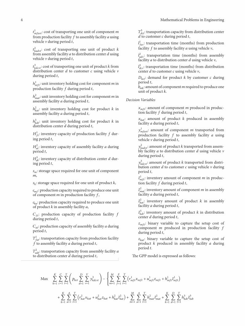
Furthermore, the following indices, parameters, and deci-sion variables are required to formulate the model:

Indices

𝑓 = 1, . . . , 𝐹: foreign supplier’s production facility,𝑎 = 1, . . . , 𝐴: manufacturer’s assembly facility,𝑑 = 1, . . . , 𝐷: distribution center,𝑐 = 1, . . . , 𝐶: customer,𝑚 = 1, . . . ,𝑀: component (each product has severalcomponents),𝑘 = 1, . . . , 𝐾: product,V = 1, . . . , 𝑉: transportation vehicle,𝑡 = 1, . . . , 𝑇: time period (month).

Parameters

𝑝𝑘𝑐𝑡: market price for one unit of product 𝑘 sold tocustomer 𝑐 during period 𝑡,𝑟1𝑚𝑓𝑡

: unit production cost for component 𝑚 in pro-duction facility 𝑓 during period 𝑡,𝑟2𝑘𝑎𝑡

: unit production cost for product 𝑘 in assemblyfacility 𝑎 during period 𝑡,𝑢1𝑚𝑓𝑡

: production setup cost for component 𝑚 inproduction facility 𝑓 during period 𝑡,𝑢2𝑘𝑎𝑡

: production setup cost for product 𝑘 in assemblyfacility 𝑎 during period 𝑡,


𝑡1𝑚𝑓𝑎V𝑡: cost of transporting one unit of component 𝑚from production facility𝑓 to assembly facility 𝑎 usingvehicle V during period 𝑡,

𝑡2𝑘𝑎𝑑V𝑡: cost of transporting one unit of product 𝑘from assembly facility 𝑎 to distribution center 𝑑 usingvehicle V during period 𝑡,

𝑡3𝑘𝑑𝑐V𝑡: cost of transporting one unit of product 𝑘 fromdistribution center 𝑑 to customer 𝑐 using vehicle Vduring period 𝑡,

ℎ1𝑚𝑓𝑡

: unit inventory holding cost for component𝑚 inproduction facility 𝑓 during period 𝑡,

ℎ2𝑚𝑎𝑡

: unit inventory holding cost for component𝑚 inassembly facility 𝑎 during period 𝑡,

ℎ2𝑘𝑎𝑡

: unit inventory holding cost for product 𝑘 inassembly facility 𝑎 during period 𝑡,

ℎ3𝑘𝑑𝑡

: unit inventory holding cost for product 𝑘 indistribution center 𝑑 during period 𝑡,

𝐻1𝑓𝑡: inventory capacity of production facility 𝑓 dur-

ing period 𝑡,

𝐻2𝑎𝑡: inventory capacity of assembly facility 𝑎 during

period 𝑡,

𝐻3𝑑𝑡: inventory capacity of distribution center 𝑑 dur-

ing period 𝑡,

𝑠𝑚: storage space required for one unit of component𝑚,

𝑠𝑘: storage space required for one unit of product 𝑘,

𝑐𝑚𝑓: production capacity required to produce one unitof component𝑚 in production facility 𝑓,

𝑐𝑘𝑎: production capacity required to produce one unitof product 𝑘 in assembly facility 𝑎,

𝐶𝑓𝑡: production capacity of production facility 𝑓during period 𝑡,

𝐶𝑎𝑡: production capacity of assembly facility 𝑎 duringperiod 𝑡,

𝑇1𝑓𝑎𝑡

: transportation capacity from production facility𝑓 to assembly facility 𝑎 during period 𝑡,

𝑇2𝑎𝑑𝑡

: transportation capacity from assembly facility 𝑎to distribution center 𝑑 during period 𝑡,

𝑇3𝑑𝑐𝑡: transportation capacity from distribution center

𝑑 to customer 𝑐 during period 𝑡,𝑙1𝑓𝑎V: transportation time (months) from productionfacility 𝑓 to assembly facility 𝑎 using vehicle V,

𝑙2𝑎𝑑V: transportation time (months) from assemblyfacility 𝑎 to distribution center 𝑑 using vehicle V,𝑙3𝑑𝑐V: transportation time (months) from distributioncenter 𝑑 to customer 𝑐 using vehicle V,𝐷𝑘𝑐𝑡: demand for product 𝑘 by customer 𝑐 duringperiod 𝑡,𝑏𝑚𝑘: amount of component𝑚 required to produce oneunit of product 𝑘.

Decision Variables

𝑥𝑚𝑓𝑡: amount of component 𝑚 produced in produc-tion facility 𝑓 during period 𝑡,𝑥𝑘𝑎𝑡: amount of product 𝑘 produced in assemblyfacility 𝑎 during period 𝑡,𝑦1𝑚𝑓𝑎V𝑡: amount of component 𝑚 transported from

production facility 𝑓 to assembly facility 𝑎 usingvehicle V during period 𝑡,𝑦2𝑘𝑎𝑑V𝑡: amount of product 𝑘 transported from assem-

bly facility 𝑎 to distribution center 𝑑 using vehicle Vduring period 𝑡,𝑦3𝑘𝑑𝑐V𝑡: amount of product 𝑘 transported from distri-

bution center 𝑑 to customer 𝑐 using vehicle V duringperiod 𝑡,𝐼1𝑚𝑓𝑡

: inventory amount of component 𝑚 in produc-tion facility 𝑓 during period 𝑡,𝐼2𝑚𝑎𝑡

: inventory amount of component 𝑚 in assemblyfacility 𝑎 during period 𝑡,𝐼2𝑘𝑎𝑡

: inventory amount of product 𝑘 in assemblyfacility 𝑎 during period 𝑡,𝐼3𝑘𝑑𝑡

: inventory amount of product 𝑘 in distributioncenter 𝑑 during period 𝑡,𝑧𝑚𝑓𝑡: binary variable to capture the setup cost ofcomponent 𝑚 produced in production facility 𝑓during period 𝑡,𝑧𝑘𝑎𝑡: binary variable to capture the setup cost ofproduct 𝑘 produced in assembly facility 𝑎 duringperiod 𝑡.

The GPP model is expressed as follows:

Max𝐾

∑𝑘=1

𝐶

∑𝑐=1

𝑇

∑𝑡=1

(𝑝𝑘𝑐𝑡

𝐷

∑𝑑=1

𝑉

∑V=1𝑦3𝑘𝑑𝑐V𝑡) −

{{{

𝑀

∑𝑚=1

𝐹

∑𝑓=1

𝑇

∑𝑡=1

(𝑟1𝑚𝑓𝑡𝑥𝑚𝑓𝑡 + 𝑢

1

𝑚𝑓𝑡𝑧𝑚𝑓𝑡 + ℎ

1

𝑚𝑓𝑡𝐼1𝑚𝑓𝑡)

+𝐾

∑𝑘=1

𝐴

∑𝑎=1

𝑇

∑𝑡=1

(𝑟2𝑘𝑎𝑡𝑥𝑘𝑎𝑡 + 𝑢

2

𝑘𝑎𝑡𝑧𝑘𝑎𝑡 + ℎ

2

𝑘𝑎𝑡𝐼2𝑘𝑎𝑡) +𝑀

∑𝑚=1

𝐴

∑𝑎=1

𝑇

∑𝑡=1

ℎ2𝑚𝑎𝑡𝐼2𝑚𝑎𝑡+𝐾

∑𝑘=1

𝐷

∑𝑑=1

𝑇

∑𝑡=1

ℎ3𝑘𝑑𝑡𝐼3𝑘𝑑𝑡


+𝑀

∑𝑚=1

𝐹

∑𝑓=1

𝐴

∑𝑎=1

𝑉

∑V=1

𝑇

∑𝑡=1

𝑡1𝑚𝑓𝑎V𝑡𝑦

1

𝑚𝑓𝑎V𝑡 +𝐾

∑𝑘=1

𝐴

∑𝑎=1

𝐷

∑𝑑=1

𝑉

∑V=1

𝑇

∑𝑡=1

𝑡2𝑘𝑎𝑑V𝑡𝑦

2

𝑘𝑎𝑑V𝑡 +𝐾

∑𝑘=1

𝐷

∑𝑑=1

𝐶

∑𝑐=1

𝑉

∑V=1

𝑇

∑𝑡=1

𝑡3𝑘𝑑𝑐V𝑡𝑦3

𝑘𝑑𝑐V𝑡}}}

(1)

subject to 𝐼1𝑚𝑓𝑡= 𝐼1𝑚𝑓𝑡−1

+ 𝑥𝑚𝑓𝑡 −𝐴

∑𝑎=1

𝑉

∑V=1𝑦1𝑚𝑓𝑎V𝑡 ∀𝑚, 𝑓, 𝑡 (2)

𝐼2𝑚𝑎𝑡= 𝐼2𝑚𝑎𝑡−1

−𝐾

∑𝑘=1

𝑏𝑚𝑘𝑥𝑘𝑎𝑡 +𝐹

∑𝑓=1

𝑉

∑V=1𝑦1𝑚𝑓𝑎𝑑V𝑡−𝑙1

𝑓𝑎V∀𝑘, 𝑎, 𝑡 (3)

𝐼2𝑘𝑎𝑡= 𝐼2𝑘𝑎𝑡−1

+ 𝑥𝑘𝑎𝑡 −𝐷

∑𝑑=1

𝑉

∑V=1𝑦2𝑘𝑎𝑑V𝑡 ∀𝑘, 𝑎, 𝑡 (4)

𝐼3𝑘𝑑𝑡= 𝐼3𝑘𝑑𝑡−1

+𝐴

∑𝑎=1

𝑉

∑V=1𝑦2𝑘𝑎𝑑V𝑡−𝑙2

𝑎𝑑V−𝐶

∑𝑐=1

𝑉

∑V=1𝑦3𝑘𝑑𝑐V𝑡 ∀𝑘, 𝑑, 𝑡 (5)

𝐷

∑𝑑=1

𝑉

∑V=1𝑦3𝑘𝑑𝑐V𝑡−𝑙3

𝑑𝑐V≤ 𝐷𝑘𝑐𝑡 ∀𝑘, 𝑐, 𝑡 (6)

𝑀

∑𝑚=1

𝑐𝑚𝑓𝑥𝑚𝑓𝑡 ≤ 𝐶𝑓𝑡 ∀𝑓, 𝑡 (7)

𝐾

∑𝑘=1

𝑐𝑘𝑎𝑥𝑘𝑎𝑡 ≤ 𝐶𝑎𝑡 ∀𝑎, 𝑡 (8)

𝑥𝑚𝑓𝑡 ≤ 𝑀 ⋅ 𝑧𝑚𝑓𝑡 ∀𝑚, 𝑓, 𝑡 (9)

𝑥𝑘𝑎𝑡 ≤ 𝑀 ⋅ 𝑧𝑘𝑎𝑡 ∀𝑘, 𝑎, 𝑡 (10)

𝑀

∑𝑚=1

𝑠𝑚𝐼1

𝑚𝑓𝑡≤ 𝐻1𝑓𝑡

∀𝑓, 𝑡 (11)

𝐾

∑𝑘=1

(𝑠𝑚𝐼2

𝑚𝑎𝑡+ 𝑠𝑘𝐼2

𝑘𝑎𝑡) ≤ 𝐻2

𝑎𝑡∀𝑎, 𝑡 (12)

𝐾

∑𝑘=1

𝑠𝑘𝐼3

𝑘𝑑𝑡≤ 𝐻3𝑑𝑡

∀𝑑, 𝑡 (13)

𝑀

∑𝑚=1

𝑉

∑V=1𝑠𝑚𝑦1

𝑚𝑓𝑎V𝑡 ≤ 𝑇1

𝑓𝑎𝑡∀𝑓, 𝑎, 𝑡 (14)

𝐾

∑𝑘=1

𝑉

∑V=1𝑠𝑘𝑦2

𝑘𝑎𝑑V𝑡 ≤ 𝑇2

𝑎𝑑𝑡∀𝑎, 𝑑, 𝑡 (15)

𝐾

∑𝑘=1

𝑉

∑V=1𝑠𝑘𝑦3

𝑘𝑑𝑐V𝑡 ≤ 𝑇3

𝑑𝑐𝑡∀𝑑, 𝑐, 𝑡 (16)

𝐼1𝑚𝑓0= 0,

𝐼2𝑚𝑎0= 0,

𝐼2𝑘𝑎0= 0,

𝐼3𝑘𝑑0= 0

∀𝑚, 𝑘, 𝑓, 𝑎, 𝑑

(17)


𝑥𝑚𝑓𝑡, 𝑥𝑘𝑎𝑡, 𝐼1

𝑚𝑓𝑡, 𝐼2𝑚𝑎𝑡, 𝐼2𝑘𝑎𝑡, 𝐼3𝑘𝑑𝑡, 𝑦1𝑚𝑓𝑎V𝑡, 𝑦

2

𝑘𝑎𝑑V𝑡, 𝑦3

𝑘𝑑𝑐V𝑡 ≥ 0 ∀𝑚, 𝑘, 𝑓, 𝑎, 𝑑, 𝑐, V, 𝑡 (18)

𝑧𝑚𝑓𝑡, 𝑧𝑘𝑎𝑡 ∈ {0, 1} ∀𝑚, 𝑘, 𝑓, 𝑎, 𝑡. (19)

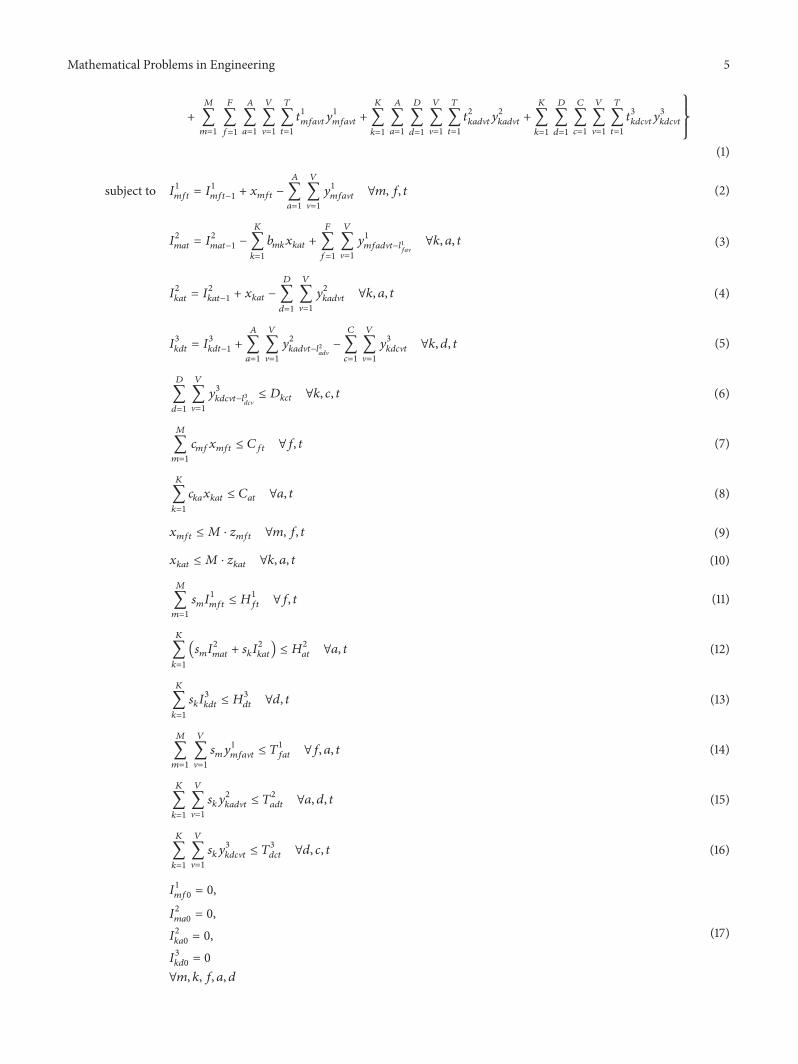
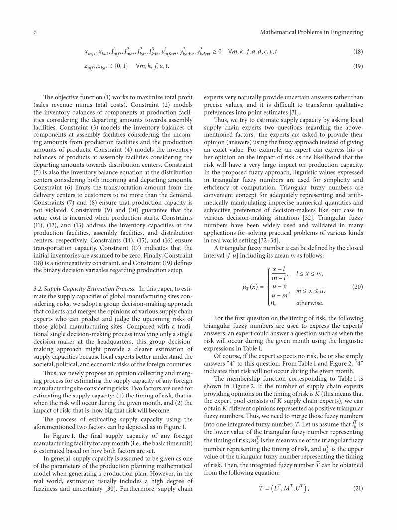
The objective function (1) works to maximize total profit(sales revenue minus total costs). Constraint (2) modelsthe inventory balances of components at production facil-ities considering the departing amounts towards assemblyfacilities. Constraint (3) models the inventory balances ofcomponents at assembly facilities considering the incom-ing amounts from production facilities and the productionamounts of products. Constraint (4) models the inventorybalances of products at assembly facilities considering thedeparting amounts towards distribution centers. Constraint(5) is also the inventory balance equation at the distributioncenters considering both incoming and departing amounts.Constraint (6) limits the transportation amount from thedelivery centers to customers to no more than the demand.Constraints (7) and (8) ensure that production capacity isnot violated. Constraints (9) and (10) guarantee that thesetup cost is incurred when production starts. Constraints(11), (12), and (13) address the inventory capacities at theproduction facilities, assembly facilities, and distributioncenters, respectively. Constraints (14), (15), and (16) ensuretransportation capacity. Constraint (17) indicates that theinitial inventories are assumed to be zero. Finally, Constraint(18) is a nonnegativity constraint, and Constraint (19) definesthe binary decision variables regarding production setup.

3.2. Supply Capacity Estimation Process. In this paper, to esti-mate the supply capacities of global manufacturing sites con-sidering risks, we adopt a group decision-making approachthat collects and merges the opinions of various supply chainexperts who can predict and judge the upcoming risks ofthose global manufacturing sites. Compared with a tradi-tional single decision-making process involving only a singledecision-maker at the headquarters, this group decision-making approach might provide a clearer estimation ofsupply capacities because local experts better understand thesocietal, political, and economic risks of the foreign countries.

Thus, we newly propose an opinion collecting and merg-ing process for estimating the supply capacity of any foreignmanufacturing site considering risks. Two factors are used forestimating the supply capacity: (1) the timing of risk, that is,when the risk will occur during the given month, and (2) theimpact of risk, that is, how big that risk will become.

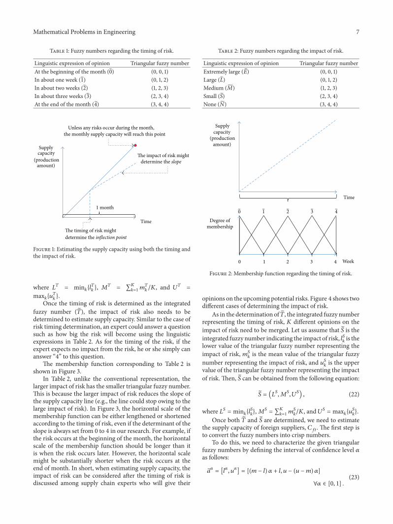
The process of estimating supply capacity using theaforementioned two factors can be depicted as in Figure 1.

In Figure 1, the final supply capacity of any foreignmanufacturing facility for anymonth (i.e., the basic time unit)is estimated based on how both factors are set.

In general, supply capacity is assumed to be given as oneof the parameters of the production planning mathematicalmodel when generating a production plan. However, in thereal world, estimation usually includes a high degree offuzziness and uncertainty [30]. Furthermore, supply chain

experts very naturally provide uncertain answers rather thanprecise values, and it is difficult to transform qualitativepreferences into point estimates [31].

Thus, we try to estimate supply capacity by asking localsupply chain experts two questions regarding the above-mentioned factors. The experts are asked to provide theiropinion (answers) using the fuzzy approach instead of givingan exact value. For example, an expert can express his orher opinion on the impact of risk as the likelihood that therisk will have a very large impact on production capacity.In the proposed fuzzy approach, linguistic values expressedin triangular fuzzy numbers are used for simplicity andefficiency of computation. Triangular fuzzy numbers areconvenient concept for adequately representing and arith-metically manipulating imprecise numerical quantities andsubjective preference of decision-makers like our case invarious decision-making situations [32]. Triangular fuzzynumbers have been widely used and validated in manyapplications for solving practical problems of various kindsin real world setting [32–34].

A triangular fuzzy number 𝑎 can be defined by the closedinterval [𝑙, 𝑢] including its mean𝑚 as follows:

𝜇𝑎 (𝑥) =

{{{{{{{{{{{

𝑥 − 𝑙

𝑚 − 𝑙, 𝑙 ≤ 𝑥 ≤ 𝑚,

𝑢 − 𝑥

𝑢 − 𝑚, 𝑚 ≤ 𝑥 ≤ 𝑢,

0, otherwise.

(20)

For the first question on the timing of risk, the followingtriangular fuzzy numbers are used to express the experts’answers: an expert could answer a question such as when therisk will occur during the given month using the linguisticexpressions in Table 1.

Of course, if the expert expects no risk, he or she simplyanswers “4” to this question. From Table 1 and Figure 2, “4”indicates that risk will not occur during the given month.

The membership function corresponding to Table 1 isshown in Figure 2. If the number of supply chain expertsproviding opinions on the timing of risk is𝐾 (this means thatthe expert pool consists of 𝐾 supply chain experts), we canobtain𝐾 different opinions represented as positive triangularfuzzy numbers.Thus, we need to merge those fuzzy numbersinto one integrated fuzzy number, 𝑇. Let us assume that 𝑙𝑇

𝑘is

the lower value of the triangular fuzzy number representingthe timing of risk,𝑚𝑇

𝑘is themean value of the triangular fuzzy

number representing the timing of risk, and 𝑢𝑇𝑘is the upper

value of the triangular fuzzy number representing the timingof risk. Then, the integrated fuzzy number �� can be obtainedfrom the following equation:

�� = (𝐿𝑇,𝑀𝑇, 𝑈𝑇) , (21)


Table 1: Fuzzy numbers regarding the timing of risk.

Linguistic expression of opinion Triangular fuzzy numberAt the beginning of the month (0) (0, 0, 1)In about one week (1) (0, 1, 2)In about two weeks (2) (1, 2, 3)In about three weeks (3) (2, 3, 4)At the end of the month (4) (3, 4, 4)

Time

Supplycapacity

(productionamount)

Unless any risks occur during the month,the monthly supply capacity will reach this point

The impact of risk mightdetermine the slope

The timing of risk mightdetermine the inflection point

1 month

Figure 1: Estimating the supply capacity using both the timing andthe impact of risk.

where 𝐿𝑇 = min𝑘{𝑙𝑇

𝑘}, 𝑀𝑇 = ∑

𝐾

𝑘=1𝑚𝑇𝑘/𝐾, and 𝑈𝑇 =

max𝑘{𝑢𝑇

𝑘}.

Once the timing of risk is determined as the integratedfuzzy number (��), the impact of risk also needs to bedetermined to estimate supply capacity. Similar to the case ofrisk timing determination, an expert could answer a questionsuch as how big the risk will become using the linguisticexpressions in Table 2. As for the timing of the risk, if theexpert expects no impact from the risk, he or she simply cananswer “4” to this question.

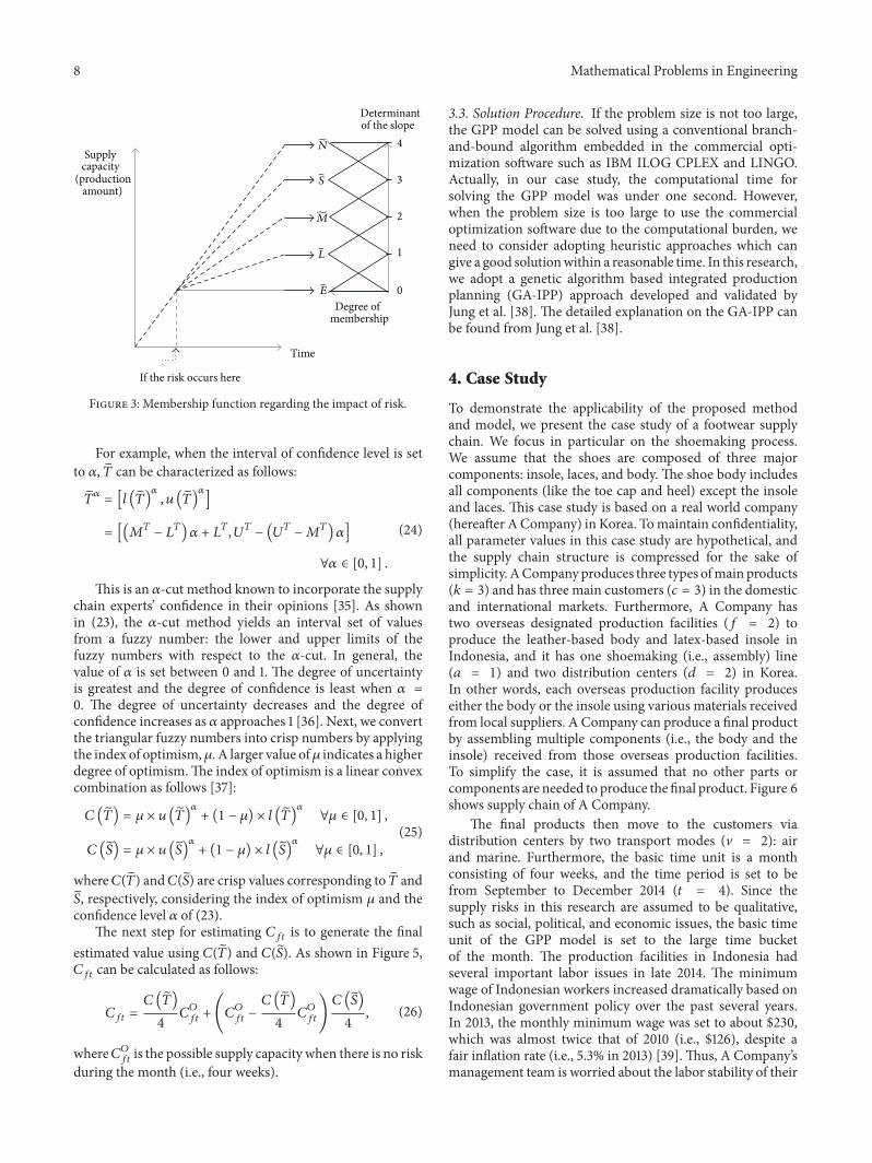
The membership function corresponding to Table 2 isshown in Figure 3.

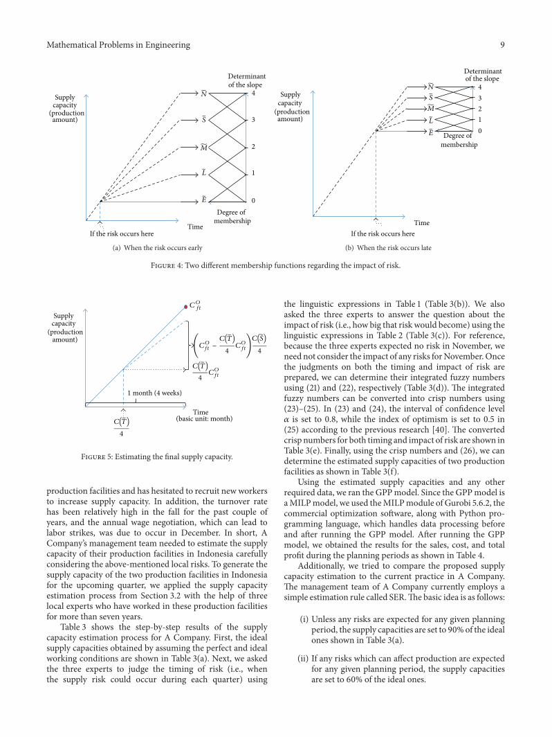
In Table 2, unlike the conventional representation, thelarger impact of risk has the smaller triangular fuzzy number.This is because the larger impact of risk reduces the slope ofthe supply capacity line (e.g., the line could stop owing to thelarge impact of risk). In Figure 3, the horizontal scale of themembership function can be either lengthened or shortenedaccording to the timing of risk, even if the determinant of theslope is always set from 0 to 4 in our research. For example, ifthe risk occurs at the beginning of the month, the horizontalscale of the membership function should be longer than itis when the risk occurs later. However, the horizontal scalemight be substantially shorter when the risk occurs at theend of month. In short, when estimating supply capacity, theimpact of risk can be considered after the timing of risk isdiscussed among supply chain experts who will give their

Table 2: Fuzzy numbers regarding the impact of risk.

Linguistic expression of opinion Triangular fuzzy numberExtremely large (𝐸) (0, 0, 1)Large (��) (0, 1, 2)Medium (��) (1, 2, 3)Small (𝑆) (2, 3, 4)None (��) (3, 4, 4)

Time

Supplycapacity

(productionamount)

0 1 2 3 4 Week

Degree ofmembership

10 2 3 4

Figure 2: Membership function regarding the timing of risk.

opinions on the upcoming potential risks. Figure 4 shows twodifferent cases of determining the impact of risk.

As in the determination of ��, the integrated fuzzy numberrepresenting the timing of risk, 𝐾 different opinions on theimpact of risk need to be merged. Let us assume that 𝑆 is theintegrated fuzzy number indicating the impact of risk, 𝑙𝑆

𝑘is the

lower value of the triangular fuzzy number representing theimpact of risk, 𝑚𝑆

𝑘is the mean value of the triangular fuzzy

number representing the impact of risk, and 𝑢𝑆𝑘is the upper

value of the triangular fuzzy number representing the impactof risk. Then, 𝑆 can be obtained from the following equation:

𝑆 = (𝐿𝑆,𝑀𝑆, 𝑈𝑆) , (22)

where 𝐿𝑆 = min𝑘{𝑙𝑆

𝑘},𝑀𝑆 = ∑𝐾

𝑘=1𝑚𝑆𝑘/𝐾, and 𝑈𝑆 = max𝑘{𝑢

𝑆

𝑘}.

Once both �� and 𝑆 are determined, we need to estimatethe supply capacity of foreign suppliers, 𝐶𝑓𝑡. The first step isto convert the fuzzy numbers into crisp numbers.

To do this, we need to characterize the given triangularfuzzy numbers by defining the interval of confidence level 𝛼as follows:

𝑎𝛼 = [𝑙𝛼, 𝑢𝛼] = [(𝑚 − 𝑙) 𝛼 + 𝑙, 𝑢 − (𝑢 − 𝑚) 𝛼]

∀𝛼 ∈ [0, 1] .(23)


Time

Supplycapacity

(productionamount)

0

1

2

3

4

Determinantof the slope

Degree ofmembership

If the risk occurs here

N

S

M

L

E

Figure 3: Membership function regarding the impact of risk.

For example, when the interval of confidence level is setto 𝛼, �� can be characterized as follows:

��𝛼 = [𝑙 (��)𝛼

, 𝑢 (��)𝛼

]

= [(𝑀𝑇 − 𝐿𝑇) 𝛼 + 𝐿𝑇, 𝑈𝑇 − (𝑈𝑇 −𝑀𝑇) 𝛼]

∀𝛼 ∈ [0, 1] .

(24)

This is an 𝛼-cut method known to incorporate the supplychain experts’ confidence in their opinions [35]. As shownin (23), the 𝛼-cut method yields an interval set of valuesfrom a fuzzy number: the lower and upper limits of thefuzzy numbers with respect to the 𝛼-cut. In general, thevalue of 𝛼 is set between 0 and 1. The degree of uncertaintyis greatest and the degree of confidence is least when 𝛼 =0. The degree of uncertainty decreases and the degree ofconfidence increases as 𝛼 approaches 1 [36]. Next, we convertthe triangular fuzzy numbers into crisp numbers by applyingthe index of optimism,𝜇. A larger value of𝜇 indicates a higherdegree of optimism.The index of optimism is a linear convexcombination as follows [37]:

𝐶 (��) = 𝜇 × 𝑢 (��)𝛼

+ (1 − 𝜇) × 𝑙 (��)𝛼

∀𝜇 ∈ [0, 1] ,

𝐶 (𝑆) = 𝜇 × 𝑢 (𝑆)𝛼

+ (1 − 𝜇) × 𝑙 (𝑆)𝛼

∀𝜇 ∈ [0, 1] ,

(25)

where𝐶(��) and𝐶(𝑆) are crisp values corresponding to �� and𝑆, respectively, considering the index of optimism 𝜇 and theconfidence level 𝛼 of (23).

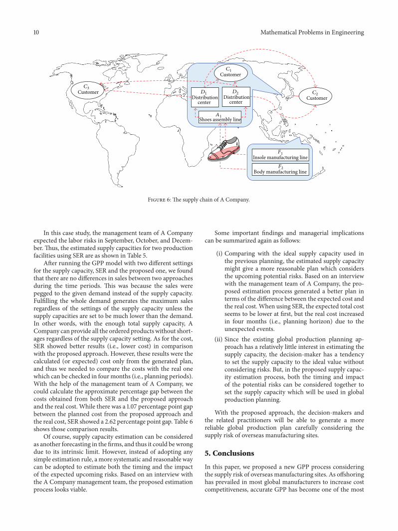
The next step for estimating 𝐶𝑓𝑡 is to generate the finalestimated value using 𝐶(��) and 𝐶(𝑆). As shown in Figure 5,𝐶𝑓𝑡 can be calculated as follows:

𝐶𝑓𝑡 =𝐶 (��)

4𝐶𝑂𝑓𝑡+ (𝐶𝑂𝑓𝑡−𝐶 (��)

4𝐶𝑂𝑓𝑡)𝐶(𝑆)

4, (26)

where𝐶𝑂𝑓𝑡is the possible supply capacity when there is no risk

during the month (i.e., four weeks).

3.3. Solution Procedure. If the problem size is not too large,the GPP model can be solved using a conventional branch-and-bound algorithm embedded in the commercial opti-mization software such as IBM ILOG CPLEX and LINGO.Actually, in our case study, the computational time forsolving the GPP model was under one second. However,when the problem size is too large to use the commercialoptimization software due to the computational burden, weneed to consider adopting heuristic approaches which cangive a good solutionwithin a reasonable time. In this research,we adopt a genetic algorithm based integrated productionplanning (GA-IPP) approach developed and validated byJung et al. [38]. The detailed explanation on the GA-IPP canbe found from Jung et al. [38].

4. Case Study

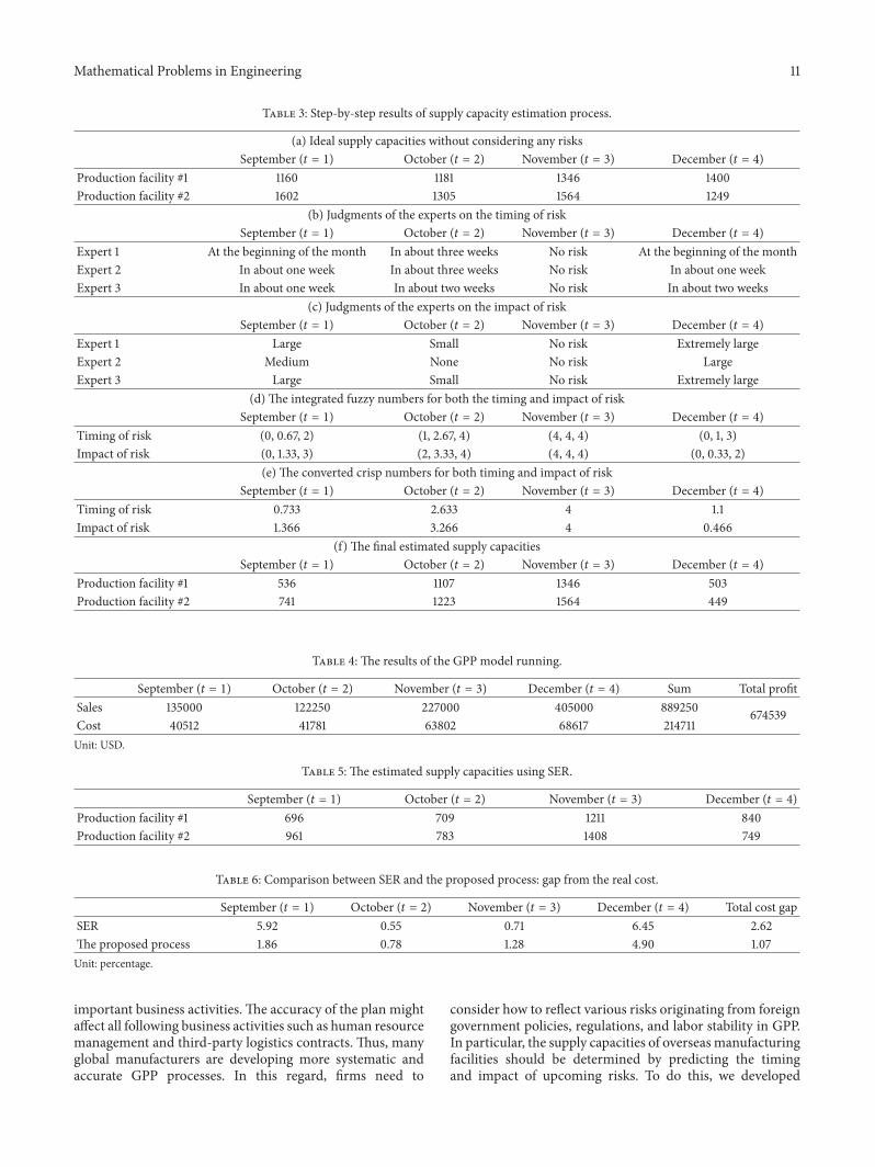
To demonstrate the applicability of the proposed methodand model, we present the case study of a footwear supplychain. We focus in particular on the shoemaking process.We assume that the shoes are composed of three majorcomponents: insole, laces, and body. The shoe body includesall components (like the toe cap and heel) except the insoleand laces. This case study is based on a real world company(hereafter ACompany) in Korea. Tomaintain confidentiality,all parameter values in this case study are hypothetical, andthe supply chain structure is compressed for the sake ofsimplicity. ACompanyproduces three types ofmain products(𝑘 = 3) and has three main customers (𝑐 = 3) in the domesticand international markets. Furthermore, A Company hastwo overseas designated production facilities (𝑓 = 2) toproduce the leather-based body and latex-based insole inIndonesia, and it has one shoemaking (i.e., assembly) line(𝑎 = 1) and two distribution centers (𝑑 = 2) in Korea.In other words, each overseas production facility produceseither the body or the insole using various materials receivedfrom local suppliers. A Company can produce a final productby assembling multiple components (i.e., the body and theinsole) received from those overseas production facilities.To simplify the case, it is assumed that no other parts orcomponents are needed to produce the final product. Figure 6shows supply chain of A Company.

The final products then move to the customers viadistribution centers by two transport modes (V = 2): airand marine. Furthermore, the basic time unit is a monthconsisting of four weeks, and the time period is set to befrom September to December 2014 (𝑡 = 4). Since thesupply risks in this research are assumed to be qualitative,such as social, political, and economic issues, the basic timeunit of the GPP model is set to the large time bucketof the month. The production facilities in Indonesia hadseveral important labor issues in late 2014. The minimumwage of Indonesian workers increased dramatically based onIndonesian government policy over the past several years.In 2013, the monthly minimum wage was set to about $230,which was almost twice that of 2010 (i.e., $126), despite afair inflation rate (i.e., 5.3% in 2013) [39]. Thus, A Company’smanagement team is worried about the labor stability of their


Time

Supplycapacity

(productionamount)


Degree ofmembership

0

1

2

3

4


N

S

M

L

E

(a) When the risk occurs early

Time

Supplycapacity

(productionamount)


Degree ofmembership

01234


N

S

M

L

E

(b) When the risk occurs late

Figure 4: Two different membership functions regarding the impact of risk.

Time(basic unit: month)

Supplycapacity

(productionamount)

1 month (4 weeks)

C(T)4

COft

C(T)4

(COft −

C(T)4

COft)C(S)

4

COft

Figure 5: Estimating the final supply capacity.

production facilities and has hesitated to recruit new workersto increase supply capacity. In addition, the turnover ratehas been relatively high in the fall for the past couple ofyears, and the annual wage negotiation, which can lead tolabor strikes, was due to occur in December. In short, ACompany’s management team needed to estimate the supplycapacity of their production facilities in Indonesia carefullyconsidering the above-mentioned local risks. To generate thesupply capacity of the two production facilities in Indonesiafor the upcoming quarter, we applied the supply capacityestimation process from Section 3.2 with the help of threelocal experts who have worked in these production facilitiesfor more than seven years.

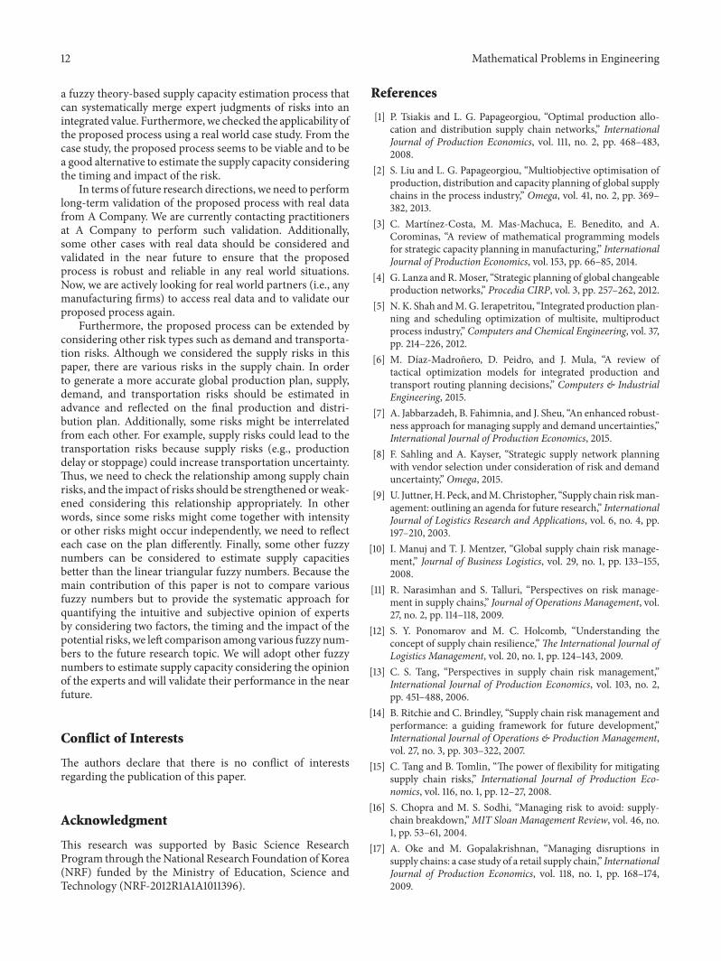
Table 3 shows the step-by-step results of the supplycapacity estimation process for A Company. First, the idealsupply capacities obtained by assuming the perfect and idealworking conditions are shown in Table 3(a). Next, we askedthe three experts to judge the timing of risk (i.e., whenthe supply risk could occur during each quarter) using

the linguistic expressions in Table 1 (Table 3(b)). We alsoasked the three experts to answer the question about theimpact of risk (i.e., how big that risk would become) using thelinguistic expressions in Table 2 (Table 3(c)). For reference,because the three experts expected no risk in November, weneed not consider the impact of any risks forNovember. Oncethe judgments on both the timing and impact of risk areprepared, we can determine their integrated fuzzy numbersusing (21) and (22), respectively (Table 3(d)). The integratedfuzzy numbers can be converted into crisp numbers using(23)–(25). In (23) and (24), the interval of confidence level𝛼 is set to 0.8, while the index of optimism is set to 0.5 in(25) according to the previous research [40]. The convertedcrisp numbers for both timing and impact of risk are shown inTable 3(e). Finally, using the crisp numbers and (26), we candetermine the estimated supply capacities of two productionfacilities as shown in Table 3(f).

Using the estimated supply capacities and any otherrequired data, we ran the GPPmodel. Since the GPPmodel isaMILPmodel, we used theMILPmodule of Gurobi 5.6.2, thecommercial optimization software, along with Python pro-gramming language, which handles data processing beforeand after running the GPP model. After running the GPPmodel, we obtained the results for the sales, cost, and totalprofit during the planning periods as shown in Table 4.

Additionally, we tried to compare the proposed supplycapacity estimation to the current practice in A Company.The management team of A Company currently employs asimple estimation rule called SER.The basic idea is as follows:

(i) Unless any risks are expected for any given planningperiod, the supply capacities are set to 90%of the idealones shown in Table 3(a).

(ii) If any risks which can affect production are expectedfor any given planning period, the supply capacitiesare set to 60% of the ideal ones.


Customer

Shoes assembly line

Insole manufacturing line

Body manufacturing line

C3

Distribution center

D1Distribution

center

D2

CustomerC1

CustomerC2

A1

F1

F2

Figure 6: The supply chain of A Company.

In this case study, the management team of A Companyexpected the labor risks in September, October, and Decem-ber. Thus, the estimated supply capacities for two productionfacilities using SER are as shown in Table 5.

After running the GPP model with two different settingsfor the supply capacity, SER and the proposed one, we foundthat there are no differences in sales between two approachesduring the time periods. This was because the sales werepegged to the given demand instead of the supply capacity.Fulfilling the whole demand generates the maximum salesregardless of the settings of the supply capacity unless thesupply capacities are set to be much lower than the demand.In other words, with the enough total supply capacity, ACompany can provide all the ordered products without short-ages regardless of the supply capacity setting. As for the cost,SER showed better results (i.e., lower cost) in comparisonwith the proposed approach. However, these results were thecalculated (or expected) cost only from the generated plan,and thus we needed to compare the costs with the real onewhich can be checked in fourmonths (i.e., planning periods).With the help of the management team of A Company, wecould calculate the approximate percentage gap between thecosts obtained from both SER and the proposed approachand the real cost. While there was a 1.07 percentage point gapbetween the planned cost from the proposed approach andthe real cost, SER showed a 2.62 percentage point gap. Table 6shows those comparison results.

Of course, supply capacity estimation can be consideredas another forecasting in the firms, and thus it could be wrongdue to its intrinsic limit. However, instead of adopting anysimple estimation rule, amore systematic and reasonable waycan be adopted to estimate both the timing and the impactof the expected upcoming risks. Based on an interview withthe A Company management team, the proposed estimationprocess looks viable.

Some important findings and managerial implicationscan be summarized again as follows:

(i) Comparing with the ideal supply capacity used inthe previous planning, the estimated supply capacitymight give a more reasonable plan which considersthe upcoming potential risks. Based on an interviewwith the management team of A Company, the pro-posed estimation process generated a better plan interms of the difference between the expected cost andthe real cost. When using SER, the expected total costseems to be lower at first, but the real cost increasedin four months (i.e., planning horizon) due to theunexpected events.

(ii) Since the existing global production planning ap-proach has a relatively little interest in estimating thesupply capacity, the decision-maker has a tendencyto set the supply capacity to the ideal value withoutconsidering risks. But, in the proposed supply capac-ity estimation process, both the timing and impactof the potential risks can be considered together toset the supply capacity which will be used in globalproduction planning.

With the proposed approach, the decision-makers andthe related practitioners will be able to generate a morereliable global production plan carefully considering thesupply risk of overseas manufacturing sites.

5. Conclusions

In this paper, we proposed a new GPP process consideringthe supply risk of overseas manufacturing sites. As offshoringhas prevailed in most global manufacturers to increase costcompetitiveness, accurate GPP has become one of the most


Table 3: Step-by-step results of supply capacity estimation process.

(a) Ideal supply capacities without considering any risksSeptember (𝑡 = 1) October (𝑡 = 2) November (𝑡 = 3) December (𝑡 = 4)

Production facility #1 1160 1181 1346 1400Production facility #2 1602 1305 1564 1249

(b) Judgments of the experts on the timing of riskSeptember (𝑡 = 1) October (𝑡 = 2) November (𝑡 = 3) December (𝑡 = 4)

Expert 1 At the beginning of the month In about three weeks No risk At the beginning of the monthExpert 2 In about one week In about three weeks No risk In about one weekExpert 3 In about one week In about two weeks No risk In about two weeks

(c) Judgments of the experts on the impact of riskSeptember (𝑡 = 1) October (𝑡 = 2) November (𝑡 = 3) December (𝑡 = 4)

Expert 1 Large Small No risk Extremely largeExpert 2 Medium None No risk LargeExpert 3 Large Small No risk Extremely large

(d) The integrated fuzzy numbers for both the timing and impact of riskSeptember (𝑡 = 1) October (𝑡 = 2) November (𝑡 = 3) December (𝑡 = 4)

Timing of risk (0, 0.67, 2) (1, 2.67, 4) (4, 4, 4) (0, 1, 3)Impact of risk (0, 1.33, 3) (2, 3.33, 4) (4, 4, 4) (0, 0.33, 2)

(e) The converted crisp numbers for both timing and impact of riskSeptember (𝑡 = 1) October (𝑡 = 2) November (𝑡 = 3) December (𝑡 = 4)

Timing of risk 0.733 2.633 4 1.1Impact of risk 1.366 3.266 4 0.466

(f) The final estimated supply capacitiesSeptember (𝑡 = 1) October (𝑡 = 2) November (𝑡 = 3) December (𝑡 = 4)

Production facility #1 536 1107 1346 503Production facility #2 741 1223 1564 449

Table 4: The results of the GPP model running.

September (𝑡 = 1) October (𝑡 = 2) November (𝑡 = 3) December (𝑡 = 4) Sum Total profitSales 135000 122250 227000 405000 889250 674539Cost 40512 41781 63802 68617 214711Unit: USD.

Table 5: The estimated supply capacities using SER.

September (𝑡 = 1) October (𝑡 = 2) November (𝑡 = 3) December (𝑡 = 4)Production facility #1 696 709 1211 840Production facility #2 961 783 1408 749

Table 6: Comparison between SER and the proposed process: gap from the real cost.

September (𝑡 = 1) October (𝑡 = 2) November (𝑡 = 3) December (𝑡 = 4) Total cost gapSER 5.92 0.55 0.71 6.45 2.62The proposed process 1.86 0.78 1.28 4.90 1.07Unit: percentage.

important business activities. The accuracy of the plan mightaffect all following business activities such as human resourcemanagement and third-party logistics contracts. Thus, manyglobal manufacturers are developing more systematic andaccurate GPP processes. In this regard, firms need to

consider how to reflect various risks originating from foreigngovernment policies, regulations, and labor stability in GPP.In particular, the supply capacities of overseas manufacturingfacilities should be determined by predicting the timingand impact of upcoming risks. To do this, we developed


a fuzzy theory-based supply capacity estimation process thatcan systematically merge expert judgments of risks into anintegrated value. Furthermore,we checked the applicability ofthe proposed process using a real world case study. From thecase study, the proposed process seems to be viable and to bea good alternative to estimate the supply capacity consideringthe timing and impact of the risk.

In terms of future research directions, we need to performlong-term validation of the proposed process with real datafrom A Company. We are currently contacting practitionersat A Company to perform such validation. Additionally,some other cases with real data should be considered andvalidated in the near future to ensure that the proposedprocess is robust and reliable in any real world situations.Now, we are actively looking for real world partners (i.e., anymanufacturing firms) to access real data and to validate ourproposed process again.

Furthermore, the proposed process can be extended byconsidering other risk types such as demand and transporta-tion risks. Although we considered the supply risks in thispaper, there are various risks in the supply chain. In orderto generate a more accurate global production plan, supply,demand, and transportation risks should be estimated inadvance and reflected on the final production and distri-bution plan. Additionally, some risks might be interrelatedfrom each other. For example, supply risks could lead to thetransportation risks because supply risks (e.g., productiondelay or stoppage) could increase transportation uncertainty.Thus, we need to check the relationship among supply chainrisks, and the impact of risks should be strengthened orweak-ened considering this relationship appropriately. In otherwords, since some risks might come together with intensityor other risks might occur independently, we need to reflecteach case on the plan differently. Finally, some other fuzzynumbers can be considered to estimate supply capacitiesbetter than the linear triangular fuzzy numbers. Because themain contribution of this paper is not to compare variousfuzzy numbers but to provide the systematic approach forquantifying the intuitive and subjective opinion of expertsby considering two factors, the timing and the impact of thepotential risks, we left comparison among various fuzzy num-bers to the future research topic. We will adopt other fuzzynumbers to estimate supply capacity considering the opinionof the experts and will validate their performance in the nearfuture.

Conflict of Interests

The authors declare that there is no conflict of interestsregarding the publication of this paper.

Acknowledgment

This research was supported by Basic Science ResearchProgram through theNational Research Foundation of Korea(NRF) funded by the Ministry of Education, Science andTechnology (NRF-2012R1A1A1011396).

References

[1] P. Tsiakis and L. G. Papageorgiou, “Optimal production allo-cation and distribution supply chain networks,” InternationalJournal of Production Economics, vol. 111, no. 2, pp. 468–483,2008.

[2] S. Liu and L. G. Papageorgiou, “Multiobjective optimisation ofproduction, distribution and capacity planning of global supplychains in the process industry,” Omega, vol. 41, no. 2, pp. 369–382, 2013.

[3] C. Martınez-Costa, M. Mas-Machuca, E. Benedito, and A.Corominas, “A review of mathematical programming modelsfor strategic capacity planning in manufacturing,” InternationalJournal of Production Economics, vol. 153, pp. 66–85, 2014.

[4] G. Lanza and R.Moser, “Strategic planning of global changeableproduction networks,” Procedia CIRP, vol. 3, pp. 257–262, 2012.

[5] N. K. Shah andM.G. Ierapetritou, “Integrated production plan-ning and scheduling optimization of multisite, multiproductprocess industry,” Computers and Chemical Engineering, vol. 37,pp. 214–226, 2012.

[6] M. Dıaz-Madronero, D. Peidro, and J. Mula, “A review oftactical optimization models for integrated production andtransport routing planning decisions,” Computers & IndustrialEngineering, 2015.

[7] A. Jabbarzadeh, B. Fahimnia, and J. Sheu, “An enhanced robust-ness approach for managing supply and demand uncertainties,”International Journal of Production Economics, 2015.

[8] F. Sahling and A. Kayser, “Strategic supply network planningwith vendor selection under consideration of risk and demanduncertainty,” Omega, 2015.

[9] U. Juttner,H. Peck, andM.Christopher, “Supply chain riskman-agement: outlining an agenda for future research,” InternationalJournal of Logistics Research and Applications, vol. 6, no. 4, pp.197–210, 2003.

[10] I. Manuj and T. J. Mentzer, “Global supply chain risk manage-ment,” Journal of Business Logistics, vol. 29, no. 1, pp. 133–155,2008.

[11] R. Narasimhan and S. Talluri, “Perspectives on risk manage-ment in supply chains,” Journal of Operations Management, vol.27, no. 2, pp. 114–118, 2009.

[12] S. Y. Ponomarov and M. C. Holcomb, “Understanding theconcept of supply chain resilience,”The International Journal ofLogistics Management, vol. 20, no. 1, pp. 124–143, 2009.

[13] C. S. Tang, “Perspectives in supply chain risk management,”International Journal of Production Economics, vol. 103, no. 2,pp. 451–488, 2006.

[14] B. Ritchie and C. Brindley, “Supply chain risk management andperformance: a guiding framework for future development,”International Journal of Operations & Production Management,vol. 27, no. 3, pp. 303–322, 2007.

[15] C. Tang and B. Tomlin, “The power of flexibility for mitigatingsupply chain risks,” International Journal of Production Eco-nomics, vol. 116, no. 1, pp. 12–27, 2008.

[16] S. Chopra and M. S. Sodhi, “Managing risk to avoid: supply-chain breakdown,”MIT Sloan Management Review, vol. 46, no.1, pp. 53–61, 2004.

[17] A. Oke and M. Gopalakrishnan, “Managing disruptions insupply chains: a case study of a retail supply chain,” InternationalJournal of Production Economics, vol. 118, no. 1, pp. 168–174,2009.


[18] I. Heckmann, T. Comes, and S. Nickel, “A critical review onsupply chain risk—definition, measure, and modeling,”Omega,vol. 52, pp. 119–132, 2015.

[19] S. C. Ellis, R. M. Henry, and J. Shockley, “Buyer perceptionsof supply disruption risk: a behavioral view and empiricalassessment,” Journal of Operations Management, vol. 28, no. 1,pp. 34–46, 2010.

[20] L. F. Escudero and P. V. Kamesam, “On solving stochasticproduction planning problems via scenario modelling,” Top,vol. 3, no. 1, pp. 69–95, 1995.

[21] S. C. H. Leung, S. O. S. Tsang, W. L. Ng, and Y. Wu, “Arobust optimization model for multi-site production planningproblem in an uncertain environment,” European Journal ofOperational Research, vol. 181, no. 1, pp. 224–238, 2007.

[22] X. Zhang, M. Prajapati, and E. Peden, “A stochastic productionplanning model under uncertain seasonal demand and marketgrowth,” International Journal of Production Research, vol. 49,no. 7, pp. 1957–1975, 2011.

[23] S. Karabuk, “Production planning under uncertainty in textilemanufacturing,” Journal of the Operational Research Society, vol.59, no. 4, pp. 510–520, 2008.

[24] D. Peidro, J. Mula, R. Poler, and F.-C. Lario, “Quantitativemodels for supply chain planning under uncertainty: a review,”International Journal of Advanced Manufacturing Technology,vol. 43, no. 3-4, pp. 400–420, 2009.

[25] S. A. Torabi and E. Hassini, “Multi-site production plan-ning integrating procurement and distribution plans in multi-echelon supply chains: an interactive fuzzy goal programmingapproach,” International Journal of Production Research, vol. 47,no. 19, pp. 5475–5499, 2009.

[26] H. Jung, “An available-to-promise process considering produc-tion and transportation uncertainties andmultiple performancemeasures,” International Journal of Production Research, vol. 50,no. 7, pp. 1780–1798, 2012.

[27] J. Wang and Y.-F. Shu, “Fuzzy decision modeling for supplychain management,” Fuzzy Sets and Systems, vol. 150, no. 1, pp.107–127, 2005.

[28] M. S. Pishvaee and S. A. Torabi, “A possibilistic programmingapproach for closed-loop supply chain network design underuncertainty,” Fuzzy Sets and Systems, vol. 161, no. 20, pp. 2668–2683, 2010.

[29] T.-F. Liang, “Application of fuzzy sets to manufacturing/dis-tribution planning decisions in supply chains,” InformationSciences, vol. 181, no. 4, pp. 842–854, 2011.

[30] A. F. Guneri, A. Yucel, and G. Ayyildiz, “An integrated fuzzy-lp approach for a supplier selection problem in supply chainmanagement,” Expert Systems with Applications, vol. 36, no. 5,pp. 9223–9228, 2009.

[31] A. H. I. Lee, H.-Y. Kang, and W.-P. Wang, “Analysis of prioritymix planning for the fabrication of semiconductors underuncertainty,”TheInternational Journal of AdvancedManufactur-ing Technology, vol. 28, no. 3-4, pp. 351–361, 2006.

[32] H. Deng, “Comparing and ranking fuzzy numbers using idealsolutions,” Applied Mathematical Modelling, vol. 38, no. 5-6, pp.1638–1646, 2014.

[33] C.-B. Cheng, “Group opinion aggregationbased on a gradingprocess: a method for constructing triangular fuzzy numbers,”Computers andMathematics with Applications, vol. 48, no. 10-11,pp. 1619–1632, 2004.

[34] D.-F. Li, “A fast approach to compute fuzzy values of matrixgames with payoffs of triangular fuzzy numbers,” European

Journal of Operational Research, vol. 223, no. 2, pp. 421–429,2012.

[35] Z. Gungor, G. Serhadlıoglu, and S. E. Kesen, “A fuzzy AHPapproach to personnel selection problem,”Applied SoftComput-ing, vol. 9, no. 2, pp. 641–646, 2009.

[36] N.-F. Pan, “Fuzzy AHP approach for selecting the suitablebridge construction method,” Automation in Construction, vol.17, no. 8, pp. 958–965, 2008.

[37] A. R. Lee, Application of modified fuzzy AHP method to analyzebolting sequence of structural joints [Ph.D. thesis], Lehigh Uni-versity, Bethlehem, Pa, USA, 1995.

[38] H. Jung, I. Song, and B. Jeong, “Genetic algorithm-basedintegrated production planning considering manufacturingpartners,”The International Journal of Advanced ManufacturingTechnology, vol. 32, no. 5-6, pp. 547–556, 2007.

[39] K. Vaswani, “Indonesia’s wage wars,” BBC News, 2013, http://www.bbc.com/news/business-21840416.

[40] H. Jung, “A fuzzy AHP-GP approach for integrated production-planning considering manufacturing partners,” Expert Systemswith Applications, vol. 38, no. 5, pp. 5833–5840, 2011.

Submit your manuscripts athttp://www.hindawi.com

Hindawi Publishing Corporationhttp://www.hindawi.com Volume 2014

MathematicsJournal of


Mathematical Problems in Engineering

Hindawi Publishing Corporationhttp://www.hindawi.com

Differential EquationsInternational Journal of

Volume 2014

Applied MathematicsJournal of


Probability and StatisticsHindawi Publishing Corporationhttp://www.hindawi.com Volume 2014

Journal of


Mathematical PhysicsAdvances in

Complex AnalysisJournal of


OptimizationJournal of


CombinatoricsHindawi Publishing Corporationhttp://www.hindawi.com Volume 2014

International Journal of


Operations ResearchAdvances in

Journal of


Function Spaces

Abstract and Applied AnalysisHindawi Publishing Corporationhttp://www.hindawi.com Volume 2014

International Journal of Mathematics and Mathematical Sciences


The Scientific World JournalHindawi Publishing Corporation http://www.hindawi.com Volume 2014


Algebra

Discrete Dynamics in Nature and Society



Decision SciencesAdvances in

Discrete MathematicsJournal of

Hindawi Publishing Corporationhttp://www.hindawi.com

Volume 2014 Hindawi Publishing Corporationhttp://www.hindawi.com Volume 2014

Stochastic AnalysisInternational Journal of

research article global production planning process

Documents