research article efficient recursive methods for partial
TRANSCRIPT
Research ArticleEfficient Recursive Methods for Partial FractionExpansion of General Rational Functions
Youneng Ma1 Jinhua Yu12 and Yuanyuan Wang1
1 Department of Electronic Engineering Fudan University Shanghai 200433 China2 Key Lab of Medical Imaging Computing and Computer Assisted Intervention of Shanghai Shanghai 200433 China
Correspondence should be addressed to Jinhua Yu jhyufudaneducn
Received 16 June 2014 Accepted 16 August 2014 Published 12 October 2014
Academic Editor Anuar Ishak
Copyright copy 2014 Youneng Ma et al This is an open access article distributed under the Creative Commons Attribution Licensewhich permits unrestricted use distribution and reproduction in any medium provided the original work is properly cited
Partial fraction expansion (pfe) is a classic technique used in many fields of pure or applied mathematics The paper focuses on thepfe of general rational functions in both factorized and expanded formNovel simple and recursive formulas for the computation ofresidues and residual polynomial coefficients are derivedThe proposed pfe methods require only simple pure-algebraic operationsin the whole computation process They do not involve derivatives when tackling proper functions and require no polynomialdivision when dealing with improper functions The methods are efficient and very easy to apply for both computer and manualcalculation Various numerical experiments confirm that the proposed methods can achieve quite desirable accuracy even for pfeof rational functions with multiple high-order poles or some tricky ill-conditioned poles
1 Introduction
Partial fraction expansion (pfe) has been a powerful toolwidely used in the field of calculus differential equationscontrol theory and some other areas of pure or appliedmathematics It is also a classic topic studied bymany scholarsover the time Though a sole solution is guaranteed it is notan easy task to perform the computation of pfe effectivelyespecially when the functions to be expanded contain high-order or ill-conditioned poles Many existing methods aredifficult to apply and can lead to considerable errors Weaim to research this classic topic and propose several novelmore efficient and simpler pfe methods for general rationalfunctions in both factorized form and expanded form
Suppose 119877(119904) = 119876(119904)119875(119904) is the rational function tobe expanded inpfe The polynomials 119875(119904) and 119876(119904) aredenominator and numerator of 119877(119904) respectively Generallya polynomial (let us say 119876(119904)) can be written in eitherexpanded form 119876(119904) = sum
119894119886119894119904119894 or factorized form 119876(119904) =
prod119894(119904 minus 119911119894)119899119894 in terms of its zeros Though theoretically equiv-
alent a method based on one of these forms may exhibitsignificant differences from the other in numerical accuracyand computational efficiency [1] In pfe problems as the poles
of 119877(119904) have to be known 119875(119904) is mostly written in factorizedform Though 119876(119904) can be written in either factorized orexpanded form the latter seems to be more in favor inpractice Most current available pfe methods are designedfor 119877(119904) with 119876(119904) written in expanded form However onemay still be motivated to design pfe methods for factorized119877(119904) For one thing many functions are originally written infactorized form A pfe method for factorized 119877(119904) can dealwith such functions directly and more efficiently thereforeit is more preferable For another under many practicalcircumstances even 119877(119904) is originally written in expandedform the zeros and poles of119877(119904) have to be obtained In otherwords 119877(119904) needs to be rewritten in factorized formThis canbe often seen in the field of system analysis and design wherepfe methods are widely used in the derivation of InverseLaplace transformation of transfer function As the zeros andpoles of the transfer function almost characterize the wholesystem they are often obtained The zero-pole plot of thetransfer function is almost used as a routine in the analysis ofsignal and system Considering that methods for factorizedfunctions can be more easily performed thus they can serveas an alternative scheme under such circumstances Someother practical reasons for the development of pfe methods
Hindawi Publishing CorporationJournal of Applied MathematicsVolume 2014 Article ID 895036 18 pageshttpdxdoiorg1011552014895036
2 Journal of Applied Mathematics
for factorized 119877(119904) are also mentioned in [2] In a word it isof significance to design methods for the pfe of 119877(119904) in bothfactorized and expanded form
The most well-known pfe method is Heavisidersquo cover-up formula It is often introduced as a textbook methodIt provides an elegant compact solution to pfe problemsand often serves as a basis for other pfe methods Howeverthis classic method requires successive differentials whenapplying to functions with high-order poles which givesrise to increasingly higher order polynomials Evaluation ofthese high-order polynomials can eventually lead to largenumerical errors [3] Another standard pfe method is themethod of undetermined coefficients This method requiresthe construction and solution of a system of equations Itcan also be very complicated and inconvenient when tacklingfunctions with high-order poles Besides the standard classicmethods many pfe methods are also proposed during thepast years Someof thesemethods tend to performbetter thanclassical methods under certain conditions However manyof them are only suitable for small-scale problems or someparticular cases and are difficult to fit into computer programTwo desirable methods are specially designed for the pfe offunctions in factorized form [3 4] In [4] Brugia developedan efficient noniterative method for pfe of functions withhigh-order poles by deriving the high-order derivative of therational functions directly without passing its lower orderones Compared with the classic methods and many otherldquotrickyrdquo methods Brugiarsquos method is more applicable andefficient It can be easily programed for computer computa-tion Linner [3] simplified Brugiarsquosmethod by using operatorsand extended it to improper functions by Laurent expansionIn [5] a modification was also made to Brugiarsquos methodwhich leads to relative simpler implementation and a reviewof many nice ldquoagedrdquo methods can also be found in [5] Mostof existing methods assume that the rational function iswritten in expanded form In [6] Karni proposed an algebraicprocedure for pfe Karnirsquos algorithm unfortunately is limitedto just those cases where the degree of the numerator isno more than the number of poles Karnirsquos method wasfurther developed yet withmuch implementation costs in [7ndash9] Pottle [10] proposed an iterative method for the digitalcomputer use but this method is subject to intolerableerrors when applied to functions with high-order poles Urazand Nagy [11] proposed a method calculating the residuesand coefficients utilizing matrix algebra Besides the aboverelatively ldquoagedrdquo methods many methods are also proposedin the recent years such as the methods in [12ndash17] Many ofthese methods are also only suitable for some particular casesand can become very complicated for large-scale problemsIn [17] Ma et al proposed an efficient pure algebraic methodfor pfe of general rational functions with high-order polesIt exhibits quite good performance and avoids long divisionwhen dealing with improper functionsThemethod does notinvolve derivative and can be coded conveniently The calcu-lation complexity of some pfemethods is discussed in [18 19]
In this paper we develop efficient recursive algebraicpfe methods for rational functions in both factorized andexpanded form Simple elegant and pure-algebraic formulasare proposed to compute the pfe coefficients The proposed
methods can be used for pfe of both proper and improperrational functions with complex poles They do not involvepolynomial division or differentiation or the solution of asystem of linear equations for the pfe of a general ratio-nal function The remainder of the paper is organized asfollows In Section 2 we focus on the pfe of functions infactorized form Brugiarsquos and Linnerrsquos methods are furtherdeveloped and simplified for much easier implementationand extended to more general cases We also develop novelsimple algebraic methods to compute the coefficients ofthe residual polynomial of improper functions that avoidspolynomial division In Section 3 we focus on the pfe ofrational function in expanded form Two novel efficientmethods are proposed Several useful compact formulasare derived for the computation of residues Two efficientmethods that avoid polynomial division are developed tocompute the coefficients of the residual polynomial InSection 4 numerical examples are provided to illustrate theusage and validity of the proposed methods followed by theconclusion in Section 5
2 Partial Faction Expansion of RationalFunctions in Factorized Form
Let the factorized rational function be
119877 (119904) =
prod119873
119895=1(119904 minus 119911
119895)119899119895
prod119872
119895=1(119904 minus 119904119895)119898119895
(1)
which is expanded as
119877 (119904) =
119864
sum
ℎ=0
119890ℎ(119904 minus 119904119888)ℎ+
119872
sum
119896=1
119898119896
sum
119871=1
119888119896119871
(119904 minus 119904119896)119871 (2)
Here 119888119896119871are the residues 119911
119895and 119904119895are the zeroes and poles of
119877(119904) respectively The poles and zeroes are assumed distinctin the whole paper 119899
119895and 119898
119895are the multiplicities of 119911
119895
and 119904119895 respectively 119873 is the number of zeros and 119872 is
the number of poles 119890ℎare the coefficients of the residual
polynomial which will be zeros for a proper 119877(119904) 119904119888is a
constant introduced to make the residual polynomial moregeneral 119904
119888is often set as zero in other articles From (1)
and (2) we can observe that the degree of the numeratorof 119877(119904) is 119881 = sum
119873
119895=1119899119895 the degree of the denominator is
119870 = sum119872
119895=1119898119895 119864 = 119881 minus 119870 In a pfe problem 119888
119896119871 119890ℎare
the unknown coefficients to be calculated We first proposea simple recursive formula to obtain the residues and thenprovide two algebraic methods for obtaining coefficients ofthe residual polynomial for an improper function
21 Computing Residues of Factorized Functions Brugia [4]developed a classic pfe method for factorized rational func-tions His method is more efficient and easier to apply forboth manual and computer calculation compared with manyother methods Here we are to further develop and simplifyBrugiarsquos method To allow for context and illumination ofdifferences and to make this paper self-contained part of
Journal of Applied Mathematics 3
Brugiarsquos method is briefly introduced below According toHeavisidersquos formula we have
119888119896119871
=
119877(119870)
119896
10038161003816100381610038161003816119904=119904119896
119870
(3)
where119870 = 119898119896minus 119871 and
119877119896 (119904) =
prod119873
119895=1(119904 minus 119911
119895)119899119895
prod119872
119895=1119895 =119896(119904 minus 119904119895)119898119895
(4)
As shown in [4] the Kth derivatives of 119877119896(119904) are
119877(119870)
119896= (119877119896119863119896)(119870minus1)
=
119870minus1
sum
119894=0
119862119894
119870minus1119877(119870minus119894minus1)
119896119863(119894)
119896 (5)
where119870 gt 0 and
119863(119894)
119896= (minus1)
119894119894(
119873
sum
119895=1
119899119895
(119904 minus 119911119895)119894+1
minus
119872
sum
119895=1
119895 =119896
119898119895
(119904 minus 119904119895)119894+1
) (6)
Here 119862119894
119898= 119898(119898 minus 119894)119894 119894 = 119894(119894 minus 1) sdot sdot sdot 1 and 0 = 1 In
the above equations we denote 119877119896(119904) by 119877
119896for simplicity of
expression Similar notations are also used for other functionsin the following partThis is Brugiarsquos main result more detailscan be found in [4] Equations (5) and (6) can generate alinear system of equations and then Gramerrsquos method canused to solve the equations to obtain the derivatives of 119877
119896(119904)
It represents a very efficient pfe method and the computerimplementation is easier to be accomplished compared withmany other existing ldquotrickyrdquo methods Here we propose asimpler method based on (3) (5) and (6) According to (3)we can obtain
119877(119894)
119896
10038161003816100381610038161003816119904=119904119896= 119894119888119896(119898119896minus119894)
(7)
Making some mathematical transformations on (6) yields
119863(119894)
119896= 119894(
119872
sum
119895=1
119895 =119896
119898119895
(119904119895minus 119904)119894+1
minus
119873
sum
119895=1
119899119895
(119911119895minus 119904)119894+1
) (8)
Here we mention that the modification on (6) to obtain (8)is relatively little but in practice it can reduce computationcosts and facilitate implementation to a considerable extentCombining (5) and (3) we have
119888119896119871
=1
119870
119870minus1
sum
119894=0
119862119894
119870minus1119877(119870minus119894minus1)
119896119863(119894)
119896
10038161003816100381610038161003816119904=119904119896 (9)
Using (7) and (8) to substitute the derivatives of 119877119896and119863
119896in
the summation of (9) yields
119888119896119871
=1
119870
119870minus1
sum
119894=0
119888119896(119898119896minus(119870minus119894minus1))
times (
119872
sum
119895=1
119895 =119896
119898119895
(119904119895minus 119904)119894+1
minus
119873
sum
119895=1
119899119895
(119911119895minus 119904)119894+1
)
1003816100381610038161003816100381610038161003816100381610038161003816100381610038161003816100381610038161003816119904=119904119896
(10)
Notice119870 = 119898119896minus 119871 Equation (10) further yields
119888119896119871
=1
119898119896minus 119871
119898119896minus119871
sum
119894=1
119888119896(119871+119894)
119894
10038161003816100381610038161003816119904=119904119896 (119871 = 119898
119896minus 1 minus1 1)
(11a)
where
119894= (
119872
sum
119895=1
119895 =119896
119898119895
(119904119895minus 119904)119894minus
119873
sum
119895=1
119899119895
(119911119895minus 119904)119894) (11b)
Here we mention that in (11a) 119871 = 119898119896minus 1 minus1 1 means
119871 = 119898119896minus1119898
119896minus2119898
119896minus3 2 1This is aMatlab denotation
which will also be used in the following part for the simplicityof expression Obviously 119888
119896119898119896= 119877119896|119904=119904119896
By using (11a)and (11b) and decreasing progressively the value of 119871 from119898119896minus 1 to 1 we can then derive other residues successively
Equations (11a) and (11b) can be implemented recursively ina straightforward way It can be achieved without the aid of acomparatively complex table as done in [3] It is much easierto apply for manual calculation than the Brugiarsquos method [4]and its modifications [3 5] Meanwhile it can be programedmore easily and reduce calculation costs
22 Computing Residual Polynomial Coefficients of FactorizedFunctions Generally as practiced by most current articleslong division or polynomial division can be used to computethe coefficients of the residual polynomial namely 119890
ℎ in
(2) However as errors will propagate at each step of thepolynomial division this scheme is not quite suitable forlarge-scale problems Moreover for a given factorized ratio-nal function the long division requires both the numeratorand denominator be rewritten in expanded form whichcan lead to additional errors and much computation costsHere we provide two novel algebraic methods to compute119890ℎthat avoid long division and the reformation of 119877(119904) The
first method described in Section 221 is obtained by furtherdeveloping LinnerrsquosmethodThe othermethod introduced inSection 222 is based on derivatives
221 Laurent Expansion Applied to Improper Rational Func-tions for Any 119904
119888 Brugiarsquos method is limited to proper func-
tions In [3] Linner proposed an excellent procedure tocompute the residual polynomial coefficient of improperfunctions by Laurent expansion Here we will further developLinnerrsquos method and obtain much simpler and more efficientcalculation formulas Linnerrsquos method demands that 119904
119888in
(2) not be equal to zeros or poles of 119877(119904) which cancause inconvenience in practice We will extend 119904
119888to any
value Linnerrsquos method is briefly introduced to allow forcontext completeness and illumination of differences Withthe substitution 119904 minus 119904
119888= 1119905 (1) transforms into
119877 (119905) = 119905minus119864119882
prod119873
119895=1(119905 minus
119895)119899119894
prod119872
119895=1(119905 minus 119904119895)119898119895
(12)
4 Journal of Applied Mathematics
where 119895= 1(119911
119895minus 119904119888) 119904119895= 1(119904
119895minus 119904119888) and 119882 is a constant
Now write
119877 (119905) = 119905minus119864 (119905) (13)
where (119905) does not include the factor 119905 In (13) applying aTaylor expansion to (119905) at 119905 = 0 we can obtain
119877 (119904) =
119867
sum
ℎ=0
(ℎ)
(0)
ℎ(119904 minus 119904119888)119864minusℎ
+ 119900 [(119904 minus 119904119888)119864minus119867
] (14)
where119867 is an integer Now expand 119877(119904) as
119877 (119904) =
119864
sum
ℎ=0
119890ℎ(119904 minus 119904119888)ℎ+ 1198772 (119904) (15)
where 1198772(119904) is the proper fraction which can be expanded as
the second part on the right-side of (2) Comparing (14) and(15) we have
119890ℎ=
(119864minusℎ)
(0)
(119864 minus ℎ) (16)
This is Linnerrsquos main result In the method the derivatives of(119905) are calculated using equations like (5) and (6) and it alsorequires 119904
119888= 119911119895and 119904119888
= 119904119895 which can cause inconvenience
in practice In the following part we first show how to extend119904119888to zeros and poles of 119877(119904) We then obtain much simpler
recursive formula for the calculation of 119890ℎ
Suppose 119904119888is the 119896th root of 119877(119904) 119904
119896 We can rewrite
119877 (119904) = (119904 minus 119904119896)minus119898119896
119877119896 (119904) (17)
where 119877119896(119904) is as defined in (4) With the substitution 119904minus 119904
119896=
1119905 in 119877119896(119904) we have
119877119896 (119905) = 119905
minus119898119896minus119864119896 (119905) (18)
where
119896 (119905) = 119882
119896
prod119873
119895=1(119905 minus
119895)119899119894
prod119872
119895=1 119895 =119896(119905 minus 119904119895)119898119895
(19)
Here 119895= 1(119911
119895minus 119904119896) 119904119895= 1(119904
119895minus 119904119896) and
119882119896=
prod119873
119895=1(119904119896minus 119911119895)119899119895
prod119872
119895=1119895 =119896(119904119896minus 119904119895)119898119895
(20)
By Taylor expanding 119896(119905) at 119905 = 0 in (18) we can obtain
119877119896 (119904) =
119867
sum
ℎ=0
(ℎ)
119896(0)
ℎ(119904 minus 119904119896)119864minusℎ+119898119896
+ 119900 [(119904 minus 119904119896)119864minus119867+119898119896
]
(21)
From (17) and (21) we have
119877 (119904) =
119867
sum
ℎ=0
(ℎ)
119896(0)
ℎ(119904 minus 119904119896)119864minusℎ
+ 119900 [(119904 minus 119904119896)119864minus119867
] (22)
Comparing (15) and (22) we can observe that
119890ℎ=
(119864minusℎ)
119896(0)
(119864 minus ℎ) (23)
Thus 119904119888is extended to the 119896th root of 119877(119904) 119904
119896 The same
procedure can be used to extend 119904119888to the 119896th zero of 119877(119904)
119911119896We can easily obtain 119890
119864by setting ℎ = 119864 in (23) or by
inspection
119890119864= 1 (24)
In Section 21 we have simplified Brugiarsquos method andderived simple recursive formula for the calculation of theresidues Notice that similar to 119877
119896(119904) 119896(119905) and (119905) are both
of factorized form and that (3) and (23) which calculate 119888119894119895
and 119890ℎ respectively are of the similar form Therefore the
aforeproposed procedure in Section 21 for the calculation of119888119894119895is also suitable for the calculation of 119890
ℎhere Take 119904
119888= 119904119896
for an instance It can be proven that
(119870)
119896= (119896119863119896)(119870minus1)
=
119870minus1
sum
119894=0
119862119894
119870minus1(119870minus119894minus1)
119896119863(119894)
119896 (25)
where
119863(119894)
119896= 119894(
119872
sum
119895=1
119895 =119896
119898119895
(119904119895minus 119905)119894+1
minus
119873
sum
119895=1
119899119895
(119895minus 119905)119894+1
) (26)
From (23) we have
(119894)
119896(0) = 119894119890
119864minus119894 (27)
According to (23) and (25) we have
119890ℎ=
1
(119864 minus ℎ)
119864minusℎminus1
sum
119894=0
119862119894
119864minusℎminus1(119864minusℎminus119894minus1)
119896119863(119894)
119896
10038161003816100381610038161003816119905=0 (28)
Using (26) and (27) to substitute the derivatives of119863119896and
119896
in (28) and then evaluating (28) at 119905 = 0 we can obtain
119890ℎ
=1
(119864 minus ℎ)
119864minusℎ
sum
119894=1
119890(ℎ+119894)
(
119872
sum
119895=1
119895 =119896
119898119895(119904119895minus 119904119896)119894
minus
119873
sum
119895=1
119899119895(119911119895minus 119904119896)119894
)
(ℎ = 119864 minus 1 minus1 0)
(29)
The same procedure can be used to compute 119890ℎwhen 119904
119888= 119904119896
In summary 119890ℎcan be calculated according to
119890ℎ=
1 (ℎ = 119864)
1
(119864 minus ℎ)
119864minusℎ
sum
119894=1
119890(ℎ+119894)
120578119894 (ℎ = 119864 minus 1 minus1 0)
(30a)
Journal of Applied Mathematics 5
where
120578119894=
119872
sum
119895=1
119895 =119896
119898119895(119904119895minus 119904119888)119894
minus
119873
sum
119895=1
119899119895(119911119895minus 119904119888)119894
(119904119888= 119904119896)
119872
sum
119895=1
119898119895(119904119895minus 119904119888)119894
minus
119873
sum
119895=1
119895 =119896
119899119895(119911119895minus 119904119888)119894
(119904119888= 119911119896)
119872
sum
119895=1
119898119895(119904119895minus 119904119888)119894
minus
119873
sum
119895=1
119899119895(119911119895minus 119904119888)119894
(otherwise)
(30b)
Equations (30a) and (30b) are such a simple and compactformula that its implementation is even very easy for handcalculation It is also much more convenient for computerprogram and requires less computation costs than the orig-inal method in [3] We just need first calculate 120578
119894using (30b)
Then 119890ℎcan be immediately obtained using (30a)
222 Computing 119890ℎthrough Derivatives We provide another
simple way to compute 119890ℎwhich also avoids the unfa-
vorable polynomial division That 119890119864
= 1 is obvi-ous Therefore we just need to obtain the remainingcoefficients 119890
0 1198901 1198902 119890
119864minus1 Notice that as the residues 119888
119896119871
can be firstly obtained in Section 21 they can be seen asknown quantities here Three conditions are considered asbelow regarding the different values of 119904
119888
(1) 119904119888
= 119911119896and 119904119888
= 119904119896 We first discuss the calculation of 119890
ℎ
when 119904119888
= 119911119896and 119904119888
= 119904119896 Here 119911
119896and 119904119896are the 119896th zero and
the 119896th pole respectively From (1) and (2) we observe thatthe coefficients 119890
0 1198901 1198902 119890
119864minus1can be obtained according
to
119890ℎ=
1
ℎ(119877(ℎ)
+ 119879(ℎ))
1003816100381610038161003816100381610038161003816119904=119904119888
(31)
where
119879 (119904) = minus
119872
sum
119896=1
119898119896
sum
119871=1
119888119896119871
(119904 minus 119904119896)119871 (32)
Here 119877 = 119877(119904) as defined in (1) and 119879 = 119879(119904) The ℎthderivative of 119879(119904) can be easily obtained as
119879(ℎ)
= (minus1)ℎminus1
119872
sum
119896=1
119898119896
sum
119895=1
119875ℎ
ℎ+119895minus1119888119896119895
(119904 minus 119904119896)119895+ℎ
(33)
where 119875119899
119898= 119898(119898 minus 119899) As 119877(119904) is of factorized form
its derivatives can be derived using functions like (4) and(5) Thus the problem is solved To further simplify theimplementation we introduce an auxiliary variable
119890ℎ=
1
ℎ119877(ℎ)1003816100381610038161003816100381610038161003816119904=119904119888
(34)
From (31) and (34) we can easily observe that
119890ℎ= 119890ℎ+
1
ℎ119879(ℎ)1003816100381610038161003816100381610038161003816119904=119904119888
(35)
Equation (34) has a similar formulation as (3) thus 119890ℎcan
be calculated and using the procedure we compute 119888119894119895in
Section 21 Accordingly we can finally obtain
119890ℎ=
119877 (119904119888) (ℎ = 0)
1
ℎ
ℎ
sum
119894=1
119890ℎminus119894
120582119894
(ℎ = 1 119864)
(36a)
where
120582119894=
119872
sum
119895=1
119898119895
(119904119895minus 119904119888)119894minus
119873
sum
119895=1
119899119895
(119911119895minus 119904119888)119894 (36b)
Here we mention that in (36a) ℎ = 1 119864 means ℎ =
1 2 3 119864 This is a Matlab denotation which will also beused in the remaining part for simplicity of expression Wecan first obtain 119890
ℎusing (36a) and (36b) then 119890
ℎcan be easily
obtained using (35) Notice the evaluation of (36b) requires119904119888
= 119911119896and 119904119888
= 119904119896 Thus other two conditions remain to be
discussed
(2) 119904119888= 119911119896 Here we discuss the condition when 119904
119888is one of
the zeros of 119877(119904) (Let us say 119911119896) Actually it will be seen that it
is more preferable to let 119904119888= 119911119896 First we rewrite 119877(119904) as
119877 (119904) = (119904 minus 119911119896)119899119896119866119896 (119904) (37)
where 119899119896is the multiplicity of 119911
119896and
119866119896 (119904) =
prod119873
119895=1119895 =119896(119904 minus 119911
119895)119899119895
prod119872
119895=1(119904 minus 119904119895)119898119895
(38)
Computing the ℎth derivative of both sides of (37) usingLeibnizrsquos formula and then setting 119904 as 119911
119896yield
119877(ℎ)
(119911119896) =
0 (ℎ lt 119899119896)
119875119899119896
ℎ119866(ℎminus119899119896)
119896(119911119896) (ℎ ge 119899
119896)
(39)
As119866119896(119904) is of factorized form its derivatives can be computed
recursively
119866(ℎminus119899119896)
119896=
119866119896
(ℎ = 119899119896)
ℎminus119899119896
sum
119894=1
119875119894minus1
ℎminus119899119896minus1119863(ℎminus119899119896minus119894)
119896119894
(ℎ gt 119899119896)
(40a)
where
119894=
119872
sum
119895=1
119898119895
(119904119895minus 119904)119894minus
119873
sum
119895=1
119895 =119896
119899119895
(119911119895minus 119904)119894 (40b)
119863(119894)
119896= 119894(
119872
sum
119895=1
119898119895
(119904119895minus 119904)119894+1
minus
119873
sum
119895=1
119895 =119896
119899119895
(119911119895minus 119904)119894+1
) (40c)
6 Journal of Applied Mathematics
Combining (31) and (39) we have
119890ℎ=
119879(ℎ)
(119911119896)
ℎ(ℎ = 0 119899
119896minus 1)
119866(ℎminus119899119896)
119896(119911119896)
(ℎ minus 119899119896)
+119879(ℎ)
(119911119896)
ℎ(ℎ = 119899
119896 119864)
(41)
Aswe did in Section 222(1) to further simply the implemen-tation we can also introduce an auxiliary variable 119890
ℎwhich
satisfies
119890ℎ= 119890ℎminus119879(ℎ)
(119911119896)
ℎ (42)
And then using the procedure that we proposed in Section 21leads to
119890ℎ=
0 (ℎ = 0 119899119896minus 1)
119866119896(119911119896) (ℎ = 119899
119896)
1
ℎ minus 119899119896
ℎ
sum
119894=1
119890ℎminus119894
119894
10038161003816100381610038161003816119904119888=119911119896(ℎ = 119899
119896+ 1 119864 minus 1)
(43)
where 119894is as defined in (40b) It can be easily observed that
the larger 119899119896is the less computation load the method will
involve Thus 119904119888can be chosen as 119911
119896= max119911
1 1199112 119911
119873
Particularly if 119899119896ge 119864 we have
119890ℎ=
119879(ℎ)
(119911119896)
ℎ (44)
(3) 119904119888= 119904119896 Last let us discuss the condition when 119904
119888= 119904119896
Here 119904119896is the 119896th pole of 119877(119904) Multiplying both sides of (2)
with (119904 minus 119904119896)119898119896 gives
119877119896 (119904) =
119864
sum
ℎ=0
119890ℎ(119904 minus 119904119896)ℎ+119898119896
minus (119904 minus 119904119896)119898119896119879 (119904) (45)
where 119877119896(119904) and 119879(119904) are as defined in (4) and (32) respec-
tively According to (45) we have
119890ℎ=
119877(ℎ+119898119896)
119896(119904) + [(119904 minus 119904
119896)119898119896119879(119904)](ℎ+119898119896)
(ℎ + 119898119896)
100381610038161003816100381610038161003816100381610038161003816100381610038161003816119904=119904119896
(46)
Based on Leibnizrsquos formula we can obtain
[(119904 minus 119904119896)119898119896119879(119904)](ℎ+119898119896)
1003816100381610038161003816100381610038161003816119904=119904119896
= 119875119898119896
ℎ+119898119896119879(ℎ)
119896
10038161003816100381610038161003816119904=119904119896 (47)
where
119879(ℎ)
119896= (minus1)
ℎminus1
119872
sum
119894=1
119894 =119896
119898119894
sum
119895=1
119875ℎ
ℎ+119895minus1119888119894119895
(119904 minus 119904119894)119895+ℎ
(48)
Let
119890ℎ=
119877(ℎ+119898119896)
119896(119904)
10038161003816100381610038161003816119904=119904119896
(ℎ + 119898119896)
(49)
Then according to (46) (47) and (49) we have
119890ℎ= 119890ℎ+119879(ℎ)
119896
ℎ
1003816100381610038161003816100381610038161003816100381610038161003816119904=119904119896
(50)
Notice that (49) has the similar formulation as (3) so thatit can also be tackled using the procedure we proposed inSection 21 We can finally obtain
119890ℎ=
1
(ℎ + 119898119896)(
ℎ
sum
119894=1
119890(ℎminus119894)
119894+
119898119896+ℎ
sum
119894=ℎ+1
119888119896(119894minusℎ)
119894)
10038161003816100381610038161003816100381610038161003816100381610038161003816119904=119904119896
(ℎ = 0 119864 minus 1)
(51)
where 119894are as defined in (11b) and 119888
119896(119894minusℎ)are residues related
to the 119896th pole It is worthy to mention that we do not haveto calculate all the
119894here if we stored them when calculating
the residues in Section 21Till this point the method for the computation of 119890
ℎis
discussed for any 119904119888 Generally it is more preferable to let 119904
119888=
119911119896in practice as this condition requires the least computation
costs
3 Partial Fraction Expansion of RationalFunctions in Expanded Form
Let the rational function in expanded form be
119877 (119904) =119876 (119904)
119875 (119904)
=sum119873
119896=0119886119896(119904 minus 1199040)119896
prod119872
119894=1(119904 minus 119904119894)119898119894
=
119864
sum
ℎ=0
119890ℎ(119904 minus 119904119888)ℎ+
119872
sum
119894=1
119898119894
sum
119895=1
119888119894119895
(119904 minus 119904119894)119895
(52)
where 119888119894119895 119890ℎare the residues and coefficients of residual poly-
nomial respectively119872 is the number of poles 119904119894are the poles
of 119877(119904) 119898119894are the multiplicities of 119904
119894 119886119896are the polynomial
coefficients of the numerator 1199040and 119904119888are constants which
are often zeros in practice and they are introduced to makethe polynomials more general Obviously the degree of thenumerator is 119873 and the degree of the denominator is 119870 =
sum119898119895 119864 = 119873 minus 119870 For a proper function 119890
ℎare zeros It can
be observed that 119877(119904) can also be expressed as
119877 (119904) =
119873
sum
119896=0
119886119896119903119896 (119904) (53)
where
119903119896 (119904) =
(119904 minus 1199040)119896
prod119872
119894=1(119904 minus 119904119894)119898119894 (54)
Suppose 119903119896(119904) can be expanded in pfe as
119903119896 (119904) =
119896minus119870
sum
ℎ=0
119890119896ℎ(119904 minus 119904119888)ℎ+
119872
sum
119894=1
119898119894
sum
119895=1
119888119896119894119895
(119904 minus 119904119894)119895 (55)
Journal of Applied Mathematics 7
Inserting (55) into (53) and then compare (53) with (52) wecan observe that the residues of 119877(119904) can be obtained as
119888119894119895=
119873
sum
119896=0
119886119896119888119896119894119895 (56)
and the residual polynomial coefficients can be calculatedaccording to
119890ℎ=
119864minusℎ
sum
119894=0
119886119870+ℎ+119894
119890(119870+ℎ+119894)ℎ
(ℎ = 0 119864) (57)
In the following part we will first show how to compute 119888119894119895
and then to calculate 119890ℎ
31 Computing Residues of Functions in Expanded Form Themethod for computation of residues can be divided into twosteps first calculate the residues of 119903
0(119904) second calculate the
residues of 119877(119904) First let us suppose 1199030(119904) can be expanded in
pfe as
1199030 (119904) =
119872
sum
119894=1
119898119894
sum
119895=1
1198880119894119895
(119904 minus 119904119894)119895 (58)
Notice that 1199030(119904) is a function of factorized form Thus it can
be expanded using the method we proposed in Section 21We just need to set the numerator as 1 in (1) namely all the119899119894= 0 in (11b) Referring to (11a) and (11b) the following
formula is immediately obtained
1198880119894119895
=1
119898119894minus 119895
119898119894minus119895
sum
119896=1
1198880119894(119895+119896)
120582119896
10038161003816100381610038161003816119904=119904119894 (119895 = 119898
119894minus 1 minus1 1)
(59a)
where
120582119896=
119872
sum
119871=1
119871 =119894
119898119871
(119904119871minus 119904)119896 (59b)
It has been proved in [17] that the residues of 119903119896(119904) and
those of 119903119896minus1
(119904) satisfy
119888119896119894119895
= 119888(119896minus1)119894(119895+1)
+ (119904119894minus 1199040) times 119888(119896minus1)119894119895
(60)
Based on the above formula all the residues of 119903119896(119904) can
be obtained Then using (56) the residues of 119877(119904) can beobtained Here we develop novel simpler formulas to derivethe residues of 119877(119904) based on the residues of 119903
0(119904) It can be
observed that the numerator of 119877(119904) can be rewritten as
119876 (119904) = 1198860+ (119904 minus 119904
0) (1198861+ (119904 minus 119904
0)
times (1198862+ (119904 minus 119904
0)
times (sdot sdot sdot 119886119873minus2
+ (119904 minus 1199040)
times (119886119873minus1
+ 119886119873(119904 minus 1199040)) sdot sdot sdot )))
(61)
According to (52) and (61) we can denote
1198910=
119886119873
119875 (119904) (62a)
119891119871=
119886119873minus119871
119875 (119904)+ (119904 minus 119904
0) 119891119871minus1
(119871 = 1 119873) (62b)
By the above denotation we have 119891119873= 119877(119904) Suppose 119891
119871can
be expanded in pfe as
119891119871=
119871minusΚ
sum
119896=0
119890119871119896(119904 minus 119904119888)119896+
119872
sum
119894=1
119898119894
sum
119895=1
119889119871119894119895
(119904 minus 119904119894)119895 (63)
Notice that 1199030(119904) = 1119875(119904) Thus according to (58) we easily
obtain the residues of 1198910
1198890119894119895
= 119886119873times 1198880119894119895 (64a)
If we have already obtained the residues of 119891119871minus1
119889(119871minus1)119894119895
referring to [17] the residues of (119904 minus 119904
0)119891119871minus1
can be obtainedas 119889(119871minus1)119894(119895+1)
+(119904119894minus1199040)times119889(119871minus1)119894119895
Therefore according to (62b)we have119889119871119894119895
= 119886119873minus119871
times 1198880119894119895
+ 119889(119871minus1)119894(119895+1)
+ (119904119894minus 1199040) times 119889(119871minus1)119894119895
(119871 = 1 119873)
(64b)
Notice that 119888119894119895= 119889119873119894119895
As 1198880119894119895
can already be calculated using(59a) and (59b) we can finally obtain the residues of 119877(119904)using formulas (64a) and (64b) successively by increasing thevalue of 119871 from 1 to 119873 Equations (64a) and (64b) can befurther developed and yield another beautiful formula
119889119871119894119895
=
119871
sum
119898=0
119886119873minus(119871minus119898)
119898
sum
119896=0
119862119896
119898(119904119894minus 1199040)1198961198880119894(119895+119898minus119896)
(65)
In (64a) (64b) and (65) if119895 + 1 gt 119898119894or 119895 + 119898 minus 119896 gt 119898
119894 the
residues 1198880119894(119895+1)
and 1198880119894(119895+119898minus119896)
do not exist and we can simplyset them as zero Formula (65) can be proved by induction asbelow
Proof of Formula (65) When 119871 = 0 (65) is reduced to (64a)Thus it is true Suppose (65) is true when 119871 = 119899 namely
119889119899119894119895
=
119899
sum
119898=0
119886119873minus(119899minus119898)
119898
sum
119896=0
119862119896
119898(119904119894minus 1199040)1198961198880119894(119895+119898minus119896)
(66)
Then according to (64b) when 119871 = 119899 + 1 we have
119889(119899+1)119894119895
= 119886119873minus(119899+1)
times 1198880119894119895
+ 119889119899119894(119895+1)
+ (119904119894minus 1199040) times 119889119899119894119895 (67)
Applying (66) to (67) yields
119889(119899+1)119894119895
= 119886119873minus(119899+1)
times 1198880119894119895
+
119899
sum
119898=0
119886119873minus(119899minus119898)
119898
sum
119896=0
119862119896
119898(119904119894minus 1199040)1198961198880119894(119895+1+119898minus119896)
+ (119904119894minus 1199040) times
119899
sum
119898=0
119886119873minus(119899minus119898)
times
119898
sum
119896=0
119862119896
119898(119904119894minus 1199040)1198961198880119894(119895+119898minus119896)
(68)
8 Journal of Applied Mathematics
From (68) we have
119889(119899+1)119894119895
= 119886119873minus(119899+1)
times 1198880119894119895
+ Λ (69)
where
Λ =
119899
sum
119898=0
119886119873minus(119899minus119898)
times
119898
sum
119896=0
119862119896
119898(119904119894minus 1199040)1198961198880119894(119895+1+119898minus119896)
+
119898
sum
119896=0
119862119896
119898(119904119894minus 1199040)119896+1
1198880119894(119895+119898minus119896)
(70a)
Equation (70a) can further lead to
Λ =
119899+1
sum
119898=1
119886119873minus(119899+1minus119898)
119898
sum
119896=0
119862119896
119898(119904119894minus 1199040)1198961198880119894(119895+119898minus119896)
(70b)
From (69) and (70b) we can finally obtain
119889(119899+1)119894119895
=
119899+1
sum
119898=0
119886119873minus(119899+1minus119898)
119898
sum
119896=0
119862119896
119898(119904119894minus 1199040)1198961198880119894(119895+119898minus119896)
(71)
Equation (71) is (65) with 119871 replaced by 119899 + 1 thus byinduction it follows that (61) is true
Setting 119871 = 119873 in (65) yields
119888119894119895=
119873
sum
119898=0
119886119898
119898
sum
119896=0
119862119896
119898(119904119894minus 1199040)1198961198880119894[119895+119898minus119896]
(72)
Equation (72) presents a direct relation between the residuesof 1199030(119904) and the residues of 119877(119904) It can be useful when
calculating a particular residue of 119877(119904)
32 Computing Residual Polynomial Coefficients of Functionsin Expanded Form We will propose novel methods tocalculate the residual polynomial coefficients namely 119890
ℎin
(52) Most existing methods calculate such coefficients usingpolynomial divisionAn algebraic procedure to calculate suchcoefficients that avoids polynomial division can be foundin [17] Here we propose two novel simpler methods whichalso avoid polynomial division We first propose a methodthrough Laurent expansion and then propose a methodthrough derivatives
321 Computation of 119890ℎthrough Laurent Expansion As
shown in (53) 119877(119904) is a sum of 119903119896(119904) if we can obtain the
residual polynomial coefficients of 119903119896(119904) 119890119896ℎ 119890ℎcan be then
obtained using (57) Obviously 119903119896(119904) will contribute to the 119890
ℎ
of 119877(119904) only when 119896 ge 119870 = sum119898119895 Thus 119896 is assumed to be no
less than119870 in this partTheproblem is then reduced to how tocalculate the 119890
119896ℎof 119903119896(119904) (119896 = 119870 119873) Notice all the 119903
119896(119904) are in
factorized form thus they can be expanded using themethodwe proposed in Section 2 However it is not advisable to doso for this can lead to cumbersome implementationActually
Table 1 The relationship between the 119890119896ℎ(119896 lt 119873) and 119890
119873ℎ
119890119896ℎ
ℎ
0 1 2 sdot sdot sdot 119864 minus 2 119864 minus 1 119864
119896
119873 1198901198730
1198901198731
1198901198732
sdot sdot sdot 119890119873(119864minus2)
119890119873(119864minus1)
119890119873119864
119873 minus 1 1198901198731
1198901198732
1198901198733
sdot sdot sdot 119890119873(119864minus1)
119890119873119864
119873 minus 2 1198901198732
1198901198732
1198901198734
sdot sdot sdot 119890119873119864
sdot sdot sdot sdot sdot sdot sdot sdot sdot sdot sdot sdot sdot sdot sdot
119870 + 2 119890119873(119864minus2)
119890119873(119864minus1)
119890119873119864
119870 + 1 119890119873(119864minus1)
119890119873119864
119870 119890119873119864
simpler methods can be obtained Referring to Section 221we can prove that
119890119896ℎ
=119903(119896minus119870minusℎ)
(0)
ℎ (ℎ = 0 119896 minus 119870) (73)
where
119903 (119905) =119882
prod119872
119895=1(119905 minus 119904119895)119898119895
(74)
Here 119904119895= 1(119904
119895minus119904119888) and119882 is a constant Let 119896 = 119896+1 in (73)
we have
119890(119896+1)ℎ
=119903(119896+1minus119870minusℎ)
(0)
ℎ (ℎ = 0 119896 + 1 minus 119870) (75)
From (73) and (75) we can observe that
119890119896ℎ
= 119890(119896+1)(ℎ+1)
(ℎ = 0 119896 minus 119870) (76)
Notice that 119890(119896+1)(ℎ+1)
are the residual polynomial coefficientsof 119903119896+1
(119904) It is clear that if we have already obtained the coeffi-cients of 119903
119896+1(119904) we can immediately obtain the coefficients of
119903119896(119904) by (76) It hereby follows that if we have already obtained
the coefficients of 119903119873(119904) 119890119873ℎ
we can successively obtain119890(119873minus1)ℎ
119890(119873minus2)ℎ
119890119870ℎ From (76) the following formula can
be obtained
119890(119870+119894)ℎ
= 119890119873(119864minus119894+ℎ)
(119894 = 0 119864 ℎ = 0 119894) (77)
Equation (77) presents the relationship between the 119890119896ℎ(119896 lt
119873) and 119890119873ℎ
which can be seen more clearly in Table 1Here we mention that we calculate the 119890
119896ℎwith 119896 decreasing
from 119873 to 119870 while the method in [17] calculates 119890119896ℎ
with119896 increasing from 119870 to 119873 It will be seen that the methodproposed here is simpler and more convenient
According to (57) and (77) we have
119890ℎ=
119864minusℎ
sum
119894=0
119886119870+ℎ+119894
119890119873(119864minus119894)
(ℎ = 0 119864) (78)
From the above analysis the whole problem is reduced tohow to obtain 119890
119873ℎ As 119903
119873(119904) is of factorized form 119890
119873ℎcan
be calculated using the methods we proposed in Section 221through Laurent expansion Thus we have
119890119873ℎ
=
1 (ℎ = 119864)
1
(119864 minus ℎ)
119864minusℎ
sum
119894=1
119890119873(ℎ+119894)
120578119894 (ℎ = 119864 minus 1 minus1 0)
(79a)
Journal of Applied Mathematics 9
where
120578119894=
119872
sum
119895=1
119895 =119896
119898119895(119904119895minus 119904119888)119894
minus 119873(119911119895minus 119904119888)119873
(119904119888= 119904119896)
119872
sum
119895=1
119898119895(119904119895minus 119904119888)119894
(119904119888= 1199040)
119872
sum
119895=1
119898119895(119904119895minus 119904119888)119894
minus 119873(119911119895minus 119904119888)119873
(otherwise)
(79b)
In summary the residual polynomial coefficients can beobtained by first using (79a) and (79b) and then using (78)
322 Computation of 119890ℎthroughDerivatives Aswe discussed
in Section 321 we just have to calculate the residual polyno-mial coefficients of 119903
119873(119904) 119890119873ℎ
and then we can obtain 119890ℎ As
119903119873(119904) is of factorized form it is also possible to use themethod
we proposed in Section 222 to calculate 119890119873ℎ
In Section 222three conditions are considered Here we only discuss themost favorable condition 119904
119888= 1199040(namely 119904
119888is a zero of 119903
119873(119904))
because firstly this condition is most suitable as it requiresthe least computation and secondly 119904
119888= 1199040
= 0 in mostpractical cases Notice that119873 gt 119870Thus we can use a formulalike (44) to calculate 119890
119873ℎwhen 119904
0is not equal to any pole of
119903119873(119904) When 119904
0is equal to a pole of 119903
119873(119904) we just need to
make a simple modification 119890119873119864
= 1 is obvious Using theprocedures in Section 222(2) we can finally have
119890119873ℎ
=119879(ℎ)
119873(119904)
ℎ
1003816100381610038161003816100381610038161003816100381610038161003816119904=119904119888
(ℎ = 1 119864 minus 1) (80)
where
119879(ℎ)
119873(119904) =
(minus1)ℎminus1
119872
sum
119894=1
119894 =119896
119898119894
sum
119895=1
119875ℎ
ℎ+119895minus1119888119873119894119895
(119904 minus 119904119894)119895+ℎ
(119904 = 119904119896)
(minus1)ℎminus1
119872
sum
119894=1
119898119894
sum
119895=1
119875ℎ
ℎ+119895minus1119888119873119894119895
(119904 minus 119904119894)119895+ℎ
(otherwise)
(81)
33 Recommendations on the Choices of Procedures In Sec-tions 31 and 32 several procedures are proposed for thecomputation of both 119890
ℎand 119888119894119895 As the calculation of 119890
ℎcan
have a relation with that of 119888119894119895 we recommend two methods
comprised of several aforeproposed procedures for improperrational functions We only suggest two typical methodswhich we consider to be preferable and suitable as below
Method 1 uses (80) and (81) to calculate 119890ℎ As we can see
from (80) and (81) the method in Section 322 requires thatwe first obtain the residues of 119903
119873(119904) Therefore we use (60)
(rather than (64a) and (64b)) to obtain the residues becausethe residues of 119903
119873(119904) are obtained in the calculation process
Method 2 uses (59a) (59b) (64a) and (64b) to obtain theresidues (79a) and (79b) and (78) to calculate 119890
ℎ It is more
preferable to use (79a) and (79b) to calculate 119890119873ℎ
as it is notbased on the residues of 119903
119873(119904)
Method 1 The following procedures comprise Method 1(a) Calculate the residues of 119903
0(119904)
1198880119894119895
=
1
prod119872
119896=1119896 =119894(119904119894minus 119904119896)119898119896
(119894 = 1 119872 119895 = 119898119894)
1
119898119894minus 119895
119898119894minus119895
sum
119896=1
1198880119894(119895+119896)
120582119896
10038161003816100381610038161003816119904=119904119894
(119894 = 1 119872 119895 = 119898119894minus 1 minus1 1)
(82)
where 120582119896= sum119872
119871=1119871 =119894(119898119871(119904119871minus 119904)119896)
(b) Calculate the residues of 119903119896(119904) using
119888119896119894119895
= 119888(119896minus1)119894(119895+1)
+ (119904119894minus 1199040) times 119888(119896minus1)119894119895
(119896 = 1 119873 119894 = 1 119872 119895 = 1 119898119894)
(83)
and then obtain the residues of 119877(119904) using 119888119894119895
=
sum119873
119896=0119886119896119888119896119894119895
(c) Calculate the residues of 119903119873(119904) using (80) and (81)
(d) Calculate the residual polynomial coefficients using(78)
Method 2 The following procedures comprise Method 2(a) Calculate the residues of 119903
0(119904) the sameway as the first
step of Method 1(b) Calculate the residues of 119877(119904) Here notice that 119888
119894119895=
119889119873119894119895
Consider
119889119871119894119895
=
119886119873times 1198880119894119895 (119871 = 0)
119886119873minus119871
times 1198880119894119895
+ 119889(119871minus1)119894(119895+1)
+ (119904119894minus 1199040) times 119889(119871minus1)119894119895
(119871 = 1 119873)
(84)
(c) Calculate the residual polynomial coefficients of 119903119873(119904)
using (79a) and (79b)(d) Calculate the residual polynomial coefficients using
(78)
4 Examples and Discussions
We provide six examples to illustrate the usage and validityof the proposed methods We use similar practices as usedin [17] to validate the efficiency of the proposed methodsfor large-scale problems Matlab codes that perform theproposed methods can be easily obtained The calculationof the numerical examples is performed by Matlab (2010b)on a PC of 32-bit word length In those examples 119904
119888and 1199040
are set as zeros if not mentioned particularly For simplicityof expression for large-scale functions of 119877(119904) we denotethe coefficients of 119877(119904) as follows array of poles 119878 =
[1199041 1199042 119904
119872] array of the multiplicities of poles 119898 =
[1198981 1198982 119898
119872] array of zeros 119885 = [119911
1 1199112 119911
119872] array
of the multiplicities of zeros 119899 = [1198991 1198992 119899
119872] polynomial
coefficients of the numerator of 119877(119904) in expanded form 119860 =
[1198860 1198861 119886
119873] The reader can refer to (1) and (52) to see
clearly the meaning of those coefficients
10 Journal of Applied Mathematics
41 Usage and Validation of Methods for Factorized Functions
Example 1 The following simple rational function is pro-vided as an instance to illustrate the usage of the methodproposed in Section 2 The example is also used by Linner in[3] One may refer to [3] to see the differences between theproposed method and Linnerrsquo method
119877 (119904) =(119904 + 3) (119904 minus 1)
3(119904 minus 2)
3(119904 minus 3)
119904(119904 + 1)4(119904 + 2)
(85)
Obviously the desired expansion is given by
119877 (119904) = 119910 (119904) minus 119879 (119904) (86)
where
119910 (119904) = 1198900+ 1198901(119904 minus 119904119888) + 1198902(119904 minus 119904119888)2
119879 (119904) = minus [1198881
119904+
11988821
(119904 + 1)+
11988822
(119904 + 1)2
+11988823
(119904 + 1)3+
11988824
(119904 + 1)4+
1198883
119904 + 2]
(87)
411 Calculation of Residues The following residues can becalculated in a direct way
1198881= 119904119877(119904)|119904=0 = minus36
11988824
= (119904 + 1)4119877(119904)
10038161003816100381610038161003816119904=minus1= 1728
1198883= (119904 + 2)119877(119904)|119904=minus2 = 4320
(88)
Using (11a) and (11b) we can calculate the remaining residuesrecursively at 119904 = minus1 Notice that minus1 is the second pole of119877(119904)First calculate
119894using (11b)
1= (
1
minus2 + 1+
1
0 + 1) minus (
1
minus3 + 1+
3
1 + 1+
3
2 + 1+
1
3 + 1)
=minus9
4
2= (
1
(minus1)2+
1
12) minus (
1
(minus2)2+
3
22+
3
32+
1
42)
=29
48
3= (
1
(minus1)3+
1
13) minus (
1
(minus2)3+
3
23+
3
33+
1
43)
=minus217
576
(89)
Then using (11a)
11988823
= 119888241= minus3888
11988822
=1
2(119888231+ 119888242) = 4896
11988821
=1
3(119888221+ 119888232+ 119888243) = minus4672
(90)
Thus we have
119879 (119904) = minus [minus36
119904+
minus4672
(119904 + 1)+
4896
(119904 + 1)2+
minus3888
(119904 + 1)3
+1728
(119904 + 1)4+4320
119904 + 2]
(91)
412 Computing Coefficients of the Residual Polynomial
(a) Method Based on Laurent Expansion Here we use themethod proposed in Section 221 Let 119904
119888be minus1 the second
pole of 119877(119904) Referring to (30a) and (30b) we have
1205781= (1 sdot (minus2 + 1) + 1 sdot (1 + 0))
minus (1 sdot (minus3 + 1) + 3 sdot (1 + 1)
+ 3 sdot (2 + 1) + 1 sdot (3 + 1)) = minus17
1205782= (1 + 1)
minus ((minus2)2+ 3 sdot 2
2+ 3 sdot 3
2+ 42) = minus57
1198902= 1 119890
1= 11989021205781= minus17
1198900=
1
2(11989011205781+ 11989021205782) = 116
(92)
Thus we have
119910 (119904) = 116 minus 17 (119904 + 1) + (119904 + 1)2 (93)
(b) Method through Derivatives Here we use the methodproposed in Section 222 to compute 119890
ℎ Obviously the
second zero of 119877(119904) 1 has the largest multiplicity of 3Thus itis chosen as 119904
119888here As 2 = 119864 lt 3 = 119899
2 we can use (44) to
derive the residual polynomial coefficients
1198900= 119879 (1) = 86
1198901= 119879(1)
(1) = minus13
(94)
Thus we have
119910 (119904) = 86 minus 13 (119904 minus 1) + (119904 minus 1)2 (95)
The complete expansion is now given by
119877 (119904) = 86 minus 13 (119904 minus 1) + (119904 minus 1)2
+minus36
119904+
minus4672
(119904 + 1)+
4896
(119904 + 1)2
+minus3888
(119904 + 1)3+
1728
(119904 + 1)4+4320
119904 + 2
(96)
Example 2 We consider here a large-scale factorizedimproper 119877(119904) with 119878 = [1 2 9 10] 119898 = [10 10
10 10] 119885 = [05 15 85 95] 119899 = [11 11 11 11]In this case the degree of the numerator is 100 The degreeof the denominator reaches 110 It is quite a large-scaleproblem Here one may see the significance of developing
Journal of Applied Mathematics 11
20 30 40 50 60 70 80 90 100
0
2
4
6
8
10
12
times1019
s
f(s)
Refpfe
(a)
20 30 40 50 60 70 80 90 100
0
02
04
06
08
1
12
times10minus15
sRe
lativ
e err
or
(b)
Figure 1 Comparison of pfe with reference solution (a) and relative error of pfe (b) in Example 2 Residual polynomial coefficients arecalculated using the method proposed in Section 221
a method which can deal with factorized 119877(119904) directly If weuse a method designed for rational functions in expandedform the reformulation of the 119877(119904) into expanded formcan lead to huge computation costs It can also introduceconsiderable additional error As done in [17] in the large-scale experiments we also do not display the expansioncoefficients because they are too many and too tedious todisplay and references of the coefficients are very difficult tofind Instead we plot the figure of 119877(119904) and that of its pfepfe(119904) together to validate the accuracy of the expansionresults And we also calculate the relative errors of pfe(119904)at different values of 119904 as |(119877(119904) minus pfe(119904))119877(119904)| (119877(119904) = 0)The results are shown in Figures 1 and 2 The figures ofthe functions are plotted within the interval [25 100] Theresidues are calculated using the methods proposed inSection 21 In Figure 1 the residual polynomial coefficientsare calculated by the method we proposed in Section 221Notice that in this figure the curve of pfe pfe is in perfectagreement with that of 119877(119904) (the reference solution)demonstrating the high accuracy of the expansion resultsAnd the relative error is nearly negligible Figure 2 presentsthe relative errors when residual polynomial coefficientsare calculated using the method proposed in Section 222Three experiments regarding the values of 119904
119888are considered
(a) 119904119888= 8 (pole of 119877(119904) method in Section 222(3) used)
(b) 119904119888
= 35 (zero of 119877(119904) method in Section 222(2)used) (c) 119904
119888= 0 (neither pole nor zero of 119877(119904) method in
Section 222(1) used) As we can see the relative errors are
also quite small demonstrating the good performance ofthose proposed methods From Figures 1 and 2 one maynotice that the method through Laurent expansion seems toperform better than the method through derivatives to someextent This is because the former calculates the residueswithout the usage of the residues
Example 3 In this example we consider a large-scalefactorized improper rational function with ill-conditionedpoles 119878 = [1000 0 01 8 9] 119898 = [8 7 7 6 6] 119885 =
[minus1 minus2 7 11 12 990] 119899 = [8 8 8 8 8 8] The degree of thenumerator is 34 The degree of the denominator is 48 119877(119904)contains three ill-conditioned high-order poles two high-order poles (0 and 01) very close to each other and an 8thpole (1000) much larger than the other poles This problemcan be rather tricky and the ill-conditioned poles may oftenlead to intolerable large errors In this example the residualpolynomial coefficients are calculated using the methodproposed in Section 221 We find the method proposed inSection 222 is not quite suitable here as some of the residuesare extremely large (nearly 1050) the manipulation of whichwill inevitably introduce large errors As can be seen inFigure 3 our method can provide quite satisfactory resultsThe figure of pfe function is in perfect agreement with thereference solution And the nearly negligible relative errorwell demonstrates themethodrsquos good performance in tacklingfunctions with ill-conditioned poles
12 Journal of Applied Mathematics
40 60 80 100
0
01
02
03
04
05
06
07
08
09
1
times10minus8
s
Rela
tive e
rror
(a)
40 60 80 100
5
55
6
65
7
75
8
times10minus11
s
Rela
tive e
rror
(b)
40 60 80 100
s
2
3
4
5
6
7
8
9
10
times10minus15
Rela
tive e
rror
(c)
Figure 2 Relative errors of pfe with residual polynomial coefficients calculated using the methods in Sections 222(3) (a) 222(2) (b) and222(1) (c) in Example 2
400 500 600 700 800 900 1000
0
1
2
3
4
5
6
7
8
9
10
s
f(s)
times1040
Refpfe
(a)
400 500 600 700 800 900 1000
s
0
02
04
06
08
1
12
14
16
18
Rela
tive e
rror
times10minus10
(b)
Figure 3 Comparison of pfe with reference solution (a) and relative error of pfe (b) in Example 3
Journal of Applied Mathematics 13
Table 2 The residues of 119903119896(119904) 119888119896
119894119895in Example 4
119896 11988811989611
11988811989621
11988811989622
11988811989631
11988811989632
1 0 minus2 1 2 1
2 0 3 minus1 minus3 minus2
3 0 minus4 1 4 4
4 0 5 minus1 minus4 minus8
5 0 minus6 1 0 16
6 0 7 minus1 16 minus32
7 0 minus8 1 minus64 64
8 0 9 minus1 192 minus128
42 Usage and Validation of Methods forFunctions in Expanded Form
Example 4 The following simple rational function is pro-vided to illustrate the usage of the method we proposed forthe pfe of functions in expanded form proposed in Section 3
119877 (119904) =8 + 3119904 + 119904
2+ 41199043+ 51199044+ 1199046+ 21199047+ 1199048
119904(119904 + 1)2(119904 + 2)
2 (97)
It can be estimated that
119877 (119904) = 1198900+ 1198901119904 + 11989021199042+ 11989021199043
+11988811
119904+
11988821
(119904 + 1)+
11988822
(119904 + 1)2+
11988831
(119904 + 2)+
11988832
(119904 + 2)2
(98)
Notice the polynomial coefficients of the numerator are 119860 =
[8 3 1 4 5 0 1 2 1] We will use the two methods to solvethis problem The procedures of the methods are describedin Section 33
Method 1 (a) Use (59a) and (59b) to expand 1199030(119904)
1199030 (119904) =
1
119904(119904 + 1)2(119904 + 2)
2
=025
119904+
1
(119904 + 1)+
minus1
(119904 + 1)2+
minus125
(119904 + 2)+
minus05
(119904 + 2)2
(99)
(b) Use (60) to calculate the residues of 119903119896(119904) 119888119896119894119895based on
the residues of 1199030(119904) The results are shown in Table 2
Then use (56) to obtain the residues of 119877(119904)
11988811
= 2 11988821
= 14
11988822
= minus7 11988831
= 69
11988832
= minus59
(100)
(c) From Table 2 we can find the residues of 1199038(119904) 1198888119894119895
1199038 (119904) =
1199048
119904(119904 + 1)2(119904 + 2)
2
= 11989080
+ 11989081119904 minus 119890821199042+ 1199043minus 1198798 (119904)
(101)
Table 3 The residual polynomial coefficients of 119903119896(119904) 119890
119896ℎin
Example 4
119890119896ℎ
ℎ
0 1 2 3
119896
8 minus72 23 minus6 1
7 minus23 minus6 1
6 minus6 1
5 1
where
1198798 (119904) = minus [
9
(119904 + 1)+
minus1
(119904 + 1)2+
192
(119904 + 2)+
minus128
(119904 + 1)2]
(102)
Using (80) and (81) we have
11989080
= 1198798 (0) = minus72
11989081
= 119879(1)
8(0) = 23
11989082
= 119879(2)
8(0) = minus4
11989083
= 1
(103)
Then referring to (78) or Table 1 we can obtain all the 119890119896ℎ
asshown in Table 3
(d) Using (78) we have 1198900= minus32 119890
1= 12 119890
2= minus4 119890
3= 1
Method 2 (a) Use (59a) and (59b) to expand 1199030(119904)
(b) Using (64a) and (64b) by increasing the value of 119871from 0 to119873 we can then obtain the residues of 119877(119904) as
11988811
= 2 11988821
= 14 11988822
= minus7
11988831
= 69 11988832
= minus59
(104)
(c) Obtain the residual polynomial coefficients of 119903119873(119904)
(here 119896 = 119873 = 8) 119890119873ℎ
using (79a) an (79b)
1199038 (119904) =
1199048
119904(119904 + 1)2(119904 + 2)
2=
1199047
(119904 + 1)2(119904 + 2)
2
= minus72 + 23119904 minus 61199042+ 1199043+ 1198798 (119904)
(105)
where 1198798(119904) is proper residual fraction Then using (78) or
Table 1 we can obtain all the 119890119896ℎ
as shown in Table 3(d) Finally using (78) we have 119890
0= minus32 119890
1= 12 119890
2= minus4
1198903= 1Thus the desired expansion is
119877 (119904) = minus32 + 12119904 minus 41199042+ 1199043
+2
119904+
14
(119904 + 1)+
minus7
(119904 + 1)2+
69
(119904 + 2)+
minus59
(119904 + 2)2
(106)
Example 5 In this example we consider a large-scale rationalfunction in expanded form The example has also beenused in [17] Thus one can make a comparison betweenthe performance of the proposed methods and the method
14 Journal of Applied Mathematics
20 40 60 80 100 120
0
2
4
6
8
10
12
times1048
s
f(s)
RefMethod 1
Method 2
(a)
20 40 60 80 100 120
s
2
4
6
8
10
12
14
16
Rela
tive e
rror
times10minus3
(b)
Rela
tive e
rror
20 40 60 80 100 120
0
1
2
3
4
5
6
7
times10minus16
s
(c)
Figure 4 Comparison of expansion results of the proposed methods with reference (a) and relative errors of Method 1 (b) and Method 2 (c)in Example 5
in [17] 119878 = [8 7 6 5 4 3 2 1] 119898 = [1 2 3 4 5 6 7 8]119860 = [01 02 59 6] In this case the degree of thedenominator is 36 and the degree of the numerator is 59Thetwo methods proposed in Section 3 are validated The resultsare shown in Figure 4 As shown in the figure themethodsweproposed can provide quite good results for such a large-scaleproblemThe relative error is desirable for both the methodsdemonstrating its good performance From Figures 4(b) and4(c) we can see thatMethod 2performs better thanMethod 1
Example 6 In this example we consider a proper rationalfunction in expanded form with ill-conditioned poles Thisexample is also used in [17] 119878 = [1000 3 2 1 11] 119898 =
[7 3 3 6 7] 119860 = [01 02 22] Thus 119877(119904) is a functioncontaining three ill-conditioned high-order poles two closehigh-order poles (1 and 11) and a 7th pole (1000) much largerthan the other poles Again we validate the two methodsproposed in Section 3As shown in Figure 5 ourmethods canprovide quite satisfactory results and the relative errors aresmall enough While the relative error is comparable to themethod in [17] we find that the proposed methods are morerobust As mentioned or shown in [8 9 17] the input orderof poles can have significant influence on the accuracy ofthe expansion results especially when the rational functionsto be expanded contain ill-conditioned poles However theaccuracy of our method tends to be less affected by theorder of the poles In this Example we can rearrange thesequence of poles 119878 as [1 11 2 3 1000] or other sequencesand achieve comparable accuracy as the sequence used this
Table 4 Counts of long operations above one-degree complexity fora proper function
Counts of long operations above one-degreecomplexity
Method forfactorizedfunctions(Section 221)
12(119867119872 minus119872119870) +119872119873 +1198722
Method forexpandedfunctions
Method 1 12(119867119872 minus119872119870) +1198722+ 2119881119870
Method 2 12(119867119872 minus119872119870) +1198722+ 119881119870
example while themethod in [17] does not performquitewellunder all these conditions
43 Computational Efficiency To provide an insight into thecalculation efficiency of the foregoing methods we count thenumber of long operations (multiplication and division) ofthe proposed methods Suppose that the zeroes and poles areknown and the functions to be expanded are proper We onlycalculate the main part of operations Operations of constantand119874(119899) complexity are not included Let 119881 be the degree ofnumerator of 119877(119904) 119870 = sum
119872
119894=1119898119894the degree of denominator
119872 as number of poles119867 = sum119872
119894=11198982
119894 and119873 as the number of
zeroes Table 4 presents counts of long operations above one-degree complexity for a proper function
Journal of Applied Mathematics 15
0 100 200 300 400
minus14
minus12
minus1
minus08
minus06
minus04
minus02
0
times10minus14
f(s)
s
RefMethod 1
Method 2
(a)
0 100 200 300 4000
05
1
15
2
25
3
35
times10minus6
s
Rela
tive e
rror
(b)
times10minus6
s
0 100 200 300 400
0
05
1
15
2
25
3
Rela
tive e
rror
(c)
Figure 5 Comparison of expansion results of the proposed methods with reference (a) and relative errors of Method 1 (b) and Method 2 (c)in Example 6
Table 5 Calculation time of large-scale examples
Example 2 Example 3 Example 5 Example 6
Calculation time (s) 00446 00384 00752 (Method 1)00172 (Method 2)
00160 (Method 1)00155 (Method 2)
The calculation time of the examples can also provide aninsight into the efficiency of the methods The calculationtime of the examples is displayed in Table 5 Overall we caneasily notice that the computing time for each method isvery small which demonstrates their good computationalefficiency For factorized Examples (Examples 2 and 3)we only provide the results when the residual polynomialcoefficients are calculated by the method we proposed inSection 221 in Table 5 If the residual polynomial coefficientsare calculated using the methods in Section 222 the cal-culation time is between 006 s and 007 s for Example 2 InExample 3 methods in Section 222 perform poorly and arenot applicable Obviously method in Section 221 is morecomputational efficient and accurate than the methods inSection 222 Thus for factorized function we recommendpfe algorithm (see Algorithm 1) using (11a) and (11b) tocalculate residues and (30a) and (30b) to calculate residuesto achieve the best performance
For functions in expanded form both methods performwell for the proper function (Example 6) The calculationtime is less than 002 s for such a large-scale tricky problemwhich proves their good calculation efficiency In Example 5which involves an improper function though both perform
well Method 2 is obviously more efficient as it uses less than14 of the time of Method 1 Meanwhile from the expansionresults we can also findMethod 2 can producemore accurateresults thanMethod 1 for improper functionsThus it is morepreferable in practical use The algorithm for Method 2 isprovided in Algorithm 2
44 Discussions We would like to discuss some other issuesabout the usage and numerical validation of the proposedmethods Firstly in the experiments we define relative erroras |(119877(119904)minuspfe(119904))119877(119904)| to estimate quantitatively the accuracyof the expansion results This criterion is valid because theoriginal function and its pfe are supposed to be theoreticallyequivalentThere is no doubt that themore coherent their fig-ures are themore accurate the expansion results areHoweverincoherence between the figures does not always indicatelow-accuracy results The errors calculated by this definitionare not the exact errors of the expansion methods Theactual errors can be much smaller than those shown in thefigures especially when ill-conditioned poles are involvedThis is because that in floating point arithmetic evaluationof partial fraction functions itself (even when the expansionresult is 100 correct) can lead to considerably large even
16 Journal of Applied Mathematics
Step 1 calculate ckmkdirectly
For 119896 = 1 119872
119888119896119898119896
=
prod119873
119895=1(119904119896minus 119911119895)119899119895
prod119872
119895=1
119895 =119896
(119904119896minus 119904119895)119898119895
EndStep 2 calculate ckL (L = mk minus 1 minus1 1) using (11a) and (11b)For 119896 = 1 119872
For 119894 = 1 119898119896minus 1
119894= (
119872
sum
119895=1
119895 =119896
119898119895
(119904119895minus 119904119896)119894minus
119873
sum
119895=1
119899119895
(119911119895minus 119904119896)119894)
EndFor 119871 = 119898
119896minus 1 minus1 1
119888119896119871
= 0
For 119894 = 1 119898119896minus 119871
119888119896119871
= 119888119896119871
+ 119888119896(119871+119894)
119894
End119888119896119871
=119888119896119871
(119898119896minus 119871)
EndEndStep 3 Calculate eh using (30a) and (30b)
Step 31 119890119864= 1
Step 32 calculate 120578119894using (30b)
For 119894 = 1 119864 minus 1
120578119894=
119872
sum
119895 = 1
119895 = 119896
119898119895(119904119895minus 119904119888)119894minus
119873
sum
119895=1
119899119895(119911119895minus 119904119888)119894
(119904119888= 119904119896)
119872
sum
119895 = 1
119898119895(119904119895minus 119904119888)119894minus
119873
sum
119895 = 1
119895 = 119896
119899119895(119911119895minus 119904119888)119894
(119904119888= 119911119896)
119872
sum
119895 = 1
119898119895(119904119895minus 119904119888)119894minus
119873
sum
119895=1
119899119895(119911119895minus 119904119888)119894
(otherwise)
EndStep 33 Calculate 119890
ℎ(ℎ = 119864 minus 1 minus1 1) using (30a)
For ℎ = 119864 minus 1 minus1 1
119890ℎ=
1
(119864 minus ℎ)
119864minusℎ
sum
119894=1
119890(ℎ+119894)
120578119894
End
Algorithm 1 Algorithm for factorized functions
intolerable errors when functions with ill-conditioned high-order poles [20] Hence it does not necessarily indicateinaccurate expansion results even when the relative errorsare comparatively large at some values of 119904 On the otherhand small relative errors can guarantee good expansionresults When using the defined relative error to validate apfe method we suggest that 119904 should not have the valuesthat make 119877(119904) have an extreme small (or extreme large)absolute value Otherwise the relative errors will inevitablygrow large due to the properties of floating point arithmeticof the computer
Secondly we provide several methods to calculatethe residual polynomial coefficients of improper 119877(119904) inSection 22 In terms of accuracy those methods performalmost equally for small- ormedian-scale problems and somelarge-scale problems But when 119877(119904) contains ill-conditionedpoles andwhen the numerator of119877(119904) hasmuch larger degreethan its denominator the method proposed in Section 221performs better than the methods proposed Section 222 asit does not use the residues as a basis
Thirdly though we proposed methods for 119877(119904) in bothfactorized and expanded form for a given factorized or
Journal of Applied Mathematics 17
Step 1 calculate residues of r0 (s) using (59a) (59b)Step 11 calculate 119888
0119894119898119894directly
For 119894 = 1 119872
1198880119894119898119894
=1
prod119872
119895=1
119895 =119894
(119904119894minus 119904119895)119898119895
EndStep 12 calculate 119888
0119894119895(119895 = 119898
119894minus 1 minus1 1) using
For 119894 = 1 119872
For 119896 = 1 119898119894minus 1
119894=
119872
sum
119871=1
119871 =119894
119898119871
(119904119871minus 119904119894)119896
EndFor 119895 = 119898
119894minus 1 minus1 1
1198880119894119895
= 0
For 119896 = 1 119898119894minus 119895
1198880119894119895
= 1198880119894119895
+ 1198880119894(119895+119896)
119896
End1198880119894119895
=
1198880119894119895
(119898119894minus 119895)
EndEnd
Step 2 calculate the residues of R(s) using (64a) and (64b)1198890119894119895
= 119886119873times 1198880119894119895 (119894 = 1 119872 119895 = 1 119898
119894)
For 119871 = 1 119873
For 119894 = 1 119872
For 119895 = 1 119898119894
119889119871119894119895
= 119886119873minus119871
times 1198880119894119895
+ 119889(119871minus1)119894(119895+1)
+ (119904119894minus 1199040) times 119889(119871minus1)119894119895
EndEnd
EndStep 3 calculate the residual polynomial coefficients of rN (s) eNh using (79a) (79b)
Step 31 119890119873119864
= 1Step 32 calculate 120578
119894using (79b)
For 119894 = 1 119864 minus 1
120578119894=
119872
sum
119895 = 1
119895 = 119896
119898119895(119904119895minus 119904119888)119894minus 119873(119911
119895minus 119904119888)119873
(119904119888= 119904119896)
119872
sum
119895=1
119898119895(119904119895minus 119904119888)119894
(119904119888= 1199040)
119872
sum
119895=1
119898119895(119904119895minus 119904119888)119894minus 119873(119911
119895minus 119904119888)119873
(otherwise)
EndStep 33 Calculate 119890
119873ℎ(ℎ = 119864 minus 1 minus1 1) using (79a)
For ℎ = 119864 minus 1 minus1 1
119890119873ℎ
=1
(119864 minus ℎ)
119864minusℎ
sum
119894=1
119890119873(ℎ+119894)
120578119894
EndStep 4 calculate the residual polynomial coefficients of R(s) using 119890
ℎ= sum119864minusℎ
119894=0119886119870+ℎ+119894
119890119873(119864minus119894)
(ℎ = 0 119864)
Algorithm 2 Algorithm for functions in expanded form
polynomial function it is not necessary to transform thefunction into another form and then performpfeWhether infactorized or expanded form the expansion results using theproposed methods are comparable Meanwhile we mention
that the methods for factorized 119877(119904) can be more easilyperformed by manual calculation
Finally 1199040and 119904119888in (2) and (52) are set as zeros in almost
all the existing articles In our paper they are introduced to
18 Journal of Applied Mathematics
generalize a polynomial They can facilitate implementationand reduce calculation in many practical situations when 119904
0
and 119904119888of119877(119904) are not zerosMoreover though a careful choice
of 1199040and 119904
119888may improve the accuracy to some extent in
certain cases it will not lead to a significant improvement ofaccuracy inmost casesThus 119904
0and 119904119888can generally be simply
set as zeros or other values at your convenience in practice
5 Conclusions
In this paper we developed efficient recursive methods forthe pfe of general rational functions in both factorized andexpanded form Simple elegant recursive formulas thatdescribe the relation of the residues and the coefficients of theresidual polynomial are obtained These methods tend to besimpler and more applicable than many existing methods forpfe of rational functions withmultiple high-order polesTheycan be easily programmed for computer use with desirableefficiency and accuracy They are also very stable whoseaccuracy is less affected by the input-order of poles Themethods are also very suitable for manual calculation
Appendix
See Algorithms 1 and 2
Conflict of Interests
The authors declare that there is no conflict of interestsregarding the publication of this paper
Acknowledgments
This work is supported by The National Natural ScienceFoundation of China (81101049 61271071) Shanghai PujiangTalent Program (12PJ1401200) Doctoral Fund of Ministry ofEducation (20110071 120019) and FudanUniversity ASIC andSystem State Key Laboratory Project (11MS007)
References
[1] R J Fateman Rational Function Computing with Poles andResidues University of California Berkeley Berkeley CalifUSA 2010 httpwwwcsberkeleyedusimfatemanpaperspolespdf
[2] F O Simons Jr and R C Harden ldquoPurely real arithmeticalgorithms optimized for the analytical and computationalevaluation of partial fraction expansionsrdquo in Proceedings of the30th Southeastern Symposium on System Theory pp 315ndash3191998
[3] L J P Linner ldquoThe computation of the kth derivative ofpolynomials and rational functions in factored form and relatedmattersrdquo IEEE Transactions on Circuits and Systems vol 21 no2 pp 233ndash236 1974
[4] O Brugia ldquoA noniterative method for the partial fractionexpansion of a rational function with high order polesrdquo SIAMReview vol 7 pp 381ndash387 1965
[5] J FMahoney and B D Sivazlian ldquoPartial fractions expansion areviewof computationalmethodology and efficiencyrdquo Journal of
Computational and Applied Mathematics vol 9 no 3 pp 247ndash269 1983
[6] S Karni ldquoEasy partial fraction expansion with multiple polesrdquoProceedings of the IEEE vol 57 pp 231ndash232 1969
[7] M F Moad and S Karni ldquoOn partial fraction expansion withmultiple poles through derivativesrdquo in Proceedings of the IEEEpp 2056ndash2058 1969
[8] F Y Chin and K Steiglitz ldquoAn O(N2) algorithm for partialfraction expansionrdquo IEEE Transactions on Circuits and Systemsvol 24 no 1 pp 42ndash45 1977
[9] D Westreich ldquoPartial fraction expansion without derivativeevaluationrdquo IEEE Transactions on Circuits and Systems vol 38no 6 pp 658ndash660 1991
[10] C Pottle ldquoOn the partial fraction expansion of a rational func-tion withmultiple poles by digital computerrdquo IEEE Transactionson Circuit Theory vol CT-11 pp 161ndash162 1964
[11] A Uraz and F L N-Nagy ldquoMatrix formulation for partial-fraction expansion of transfer functionsrdquo Journal of the FranklinInstitute vol 297 pp 81ndash87 1974
[12] S H Kung ldquoPartial fraction decomposition by divisionrdquo TheCollege Mathematics Journal vol 37 pp 132ndash134 2006
[13] R Witula and D Slota ldquoPartial fractions decompositions ofsome rational functionsrdquo Applied Mathematics and Computa-tion vol 197 no 1 pp 328ndash336 2008
[14] A Ozyapici and C S Pintea ldquoComplex partial fraction decom-positions of rational functionsrdquo Journal of Computational andApplied Mathematics vol 1 article 120 2012
[15] M I Garcia-Planas and J L Dominguez ldquoA general approachfor computing residues of partial-fraction expansion of transfermatricesrdquo WSEAS Transactions on Mathematics vol 12 pp647ndash756 2013
[16] Y K Man ldquoA cover-up approach to partial fractions with linearor irreducible quadratic factors in the denominatorsrdquo AppliedMathematics and Computation vol 219 no 8 pp 3855ndash38622012
[17] Y N Ma J H Yu and Y Y Wang ldquoAn easy pure algebraicmethod for partial expansion of rational functions with multi-ple high-order polesrdquo IEEETransactions onCircuits and SystemsI vol 61 pp 803ndash810 2014
[18] F Y Chin ldquoThe partial fraction expansion problem and itsinverserdquo SIAM Journal on Computing vol 6 no 3 pp 554ndash5621977
[19] H T Kung andDM Tong ldquoFast algorithms for partial fractiondecompositionrdquo SIAM Journal on Computing vol 6 no 3 pp582ndash593 1977
[20] D Calvetti E Gallopoulos and L Reichel ldquoIncomplete partialfractions for parallel evaluation of rational matrix functionsrdquoJournal of Computational and Applied Mathematics vol 59 no3 pp 349ndash380 1995
Submit your manuscripts athttpwwwhindawicom
Hindawi Publishing Corporationhttpwwwhindawicom Volume 2014
MathematicsJournal of
Hindawi Publishing Corporationhttpwwwhindawicom Volume 2014
Mathematical Problems in Engineering
Hindawi Publishing Corporationhttpwwwhindawicom
Differential EquationsInternational Journal of
Volume 2014
Applied MathematicsJournal of
Hindawi Publishing Corporationhttpwwwhindawicom Volume 2014
Probability and StatisticsHindawi Publishing Corporationhttpwwwhindawicom Volume 2014
Journal of
Hindawi Publishing Corporationhttpwwwhindawicom Volume 2014
Mathematical PhysicsAdvances in
Complex AnalysisJournal of
Hindawi Publishing Corporationhttpwwwhindawicom Volume 2014
OptimizationJournal of
Hindawi Publishing Corporationhttpwwwhindawicom Volume 2014
CombinatoricsHindawi Publishing Corporationhttpwwwhindawicom Volume 2014
International Journal of
Hindawi Publishing Corporationhttpwwwhindawicom Volume 2014
Operations ResearchAdvances in
Journal of
Hindawi Publishing Corporationhttpwwwhindawicom Volume 2014
Function Spaces
Abstract and Applied AnalysisHindawi Publishing Corporationhttpwwwhindawicom Volume 2014
International Journal of Mathematics and Mathematical Sciences
Hindawi Publishing Corporationhttpwwwhindawicom Volume 2014
The Scientific World JournalHindawi Publishing Corporation httpwwwhindawicom Volume 2014
Hindawi Publishing Corporationhttpwwwhindawicom Volume 2014
Algebra
Discrete Dynamics in Nature and Society
Hindawi Publishing Corporationhttpwwwhindawicom Volume 2014
Hindawi Publishing Corporationhttpwwwhindawicom Volume 2014
Decision SciencesAdvances in
Discrete MathematicsJournal of
Hindawi Publishing Corporationhttpwwwhindawicom
Volume 2014 Hindawi Publishing Corporationhttpwwwhindawicom Volume 2014
Stochastic AnalysisInternational Journal of
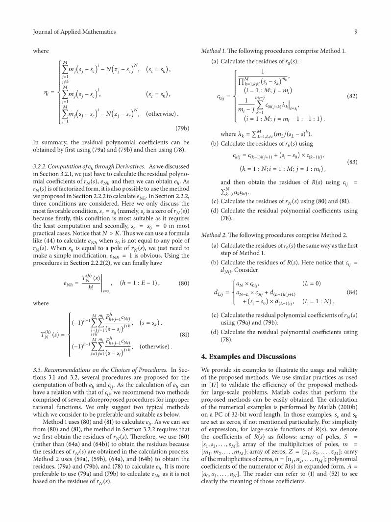
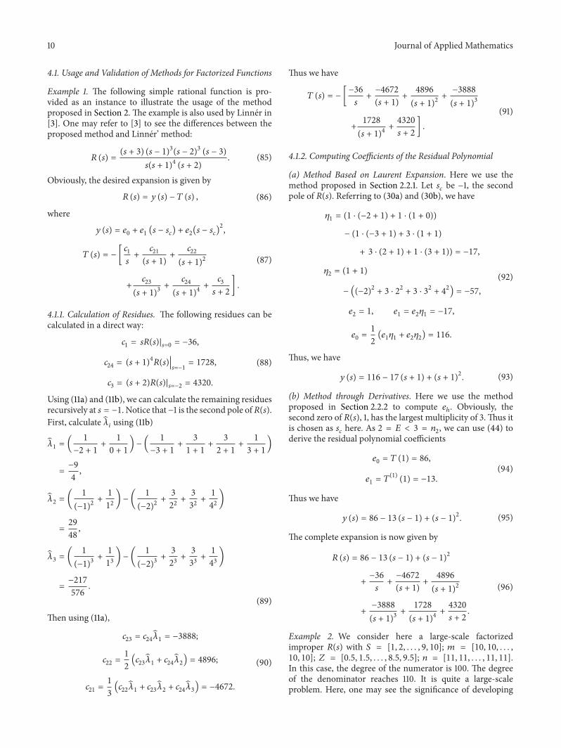
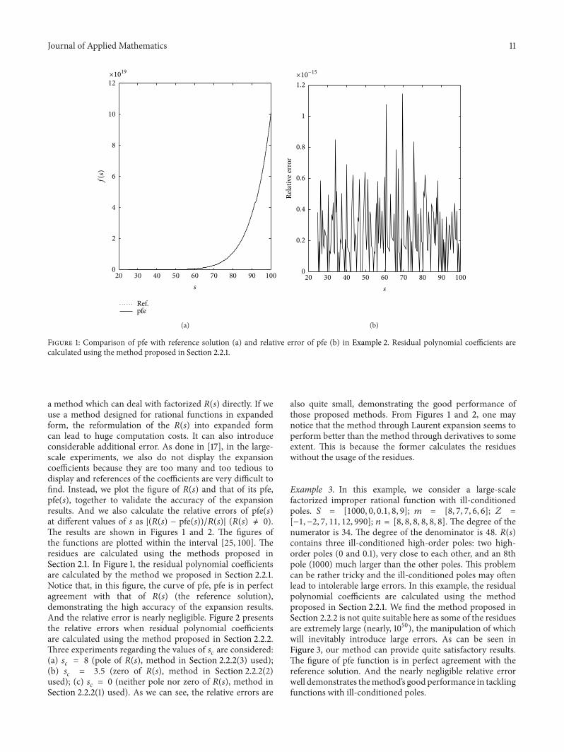
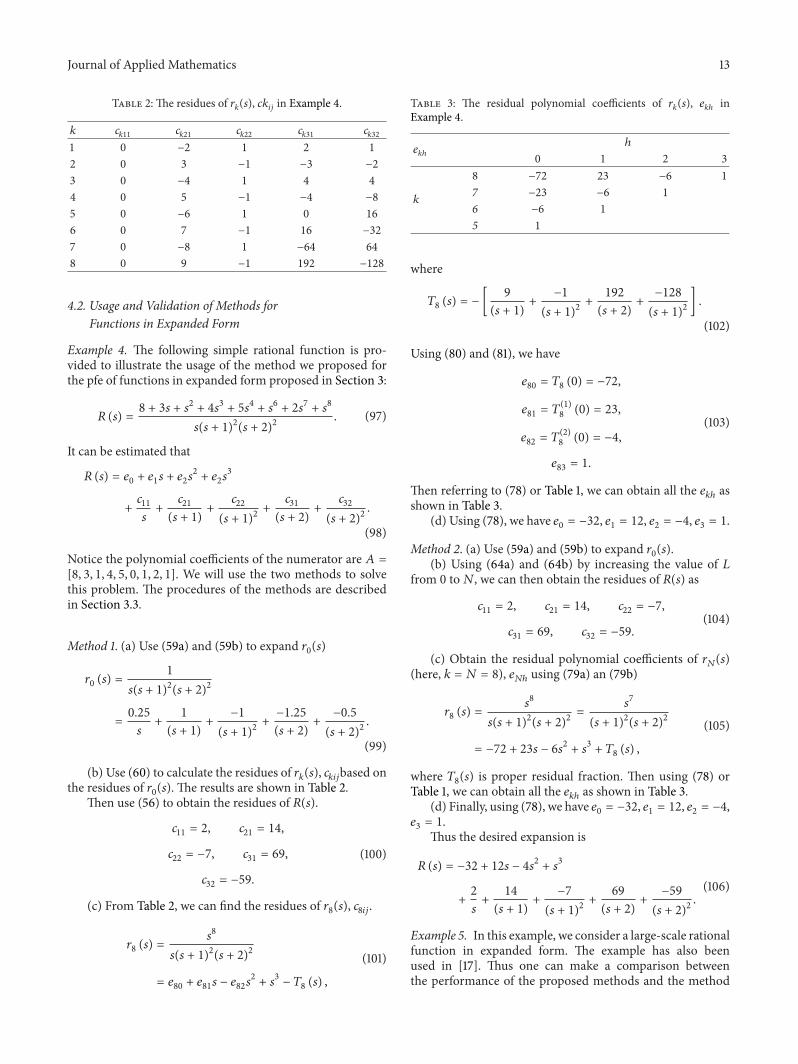
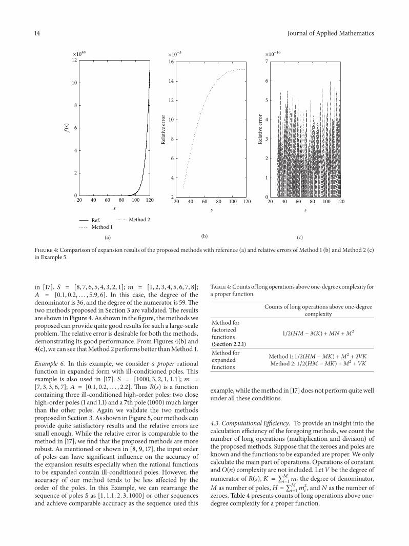
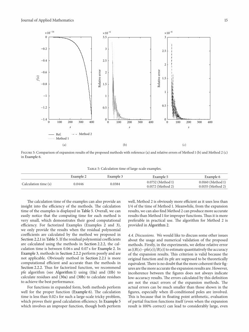
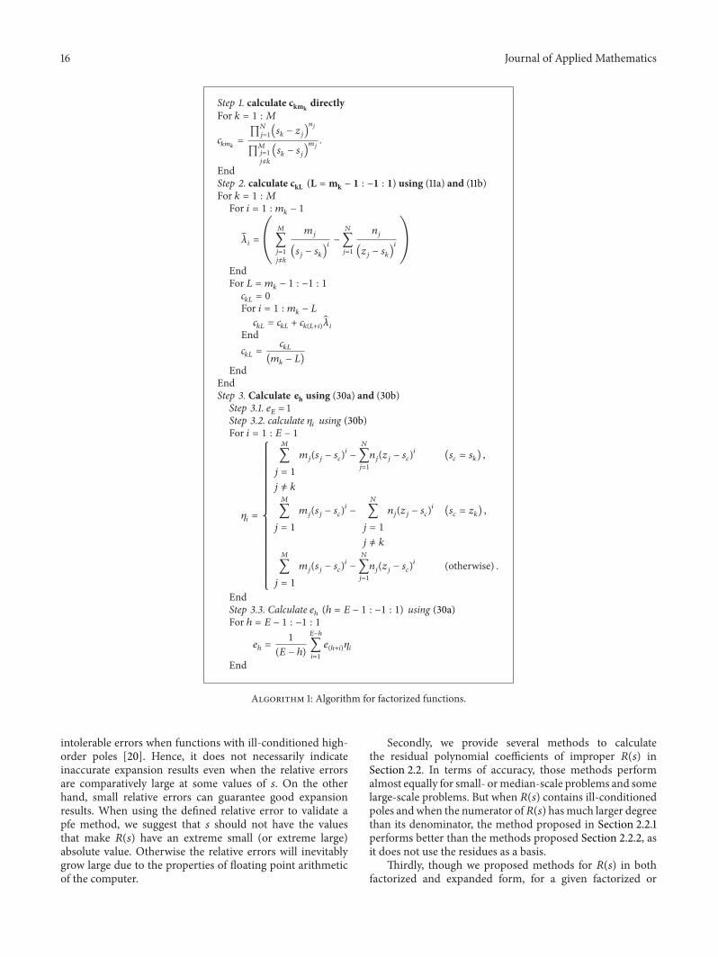
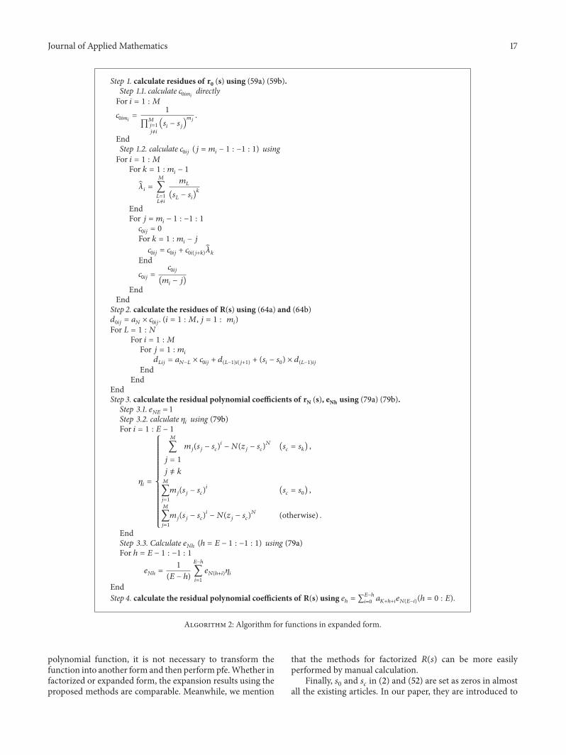