research article considering long-term characteristics iet

IET Generation, Transmission & Distribution

Research Article

Impact of optimum power factor of PV-controlled inverter on the aging and cost-effectiveness of oil-filled transformerconsidering long-term characteristics

ISSN 1751-8687Received on 15th March 2019Revised 11th June 2019Accepted on 24th June 2019E-First on 26th July 2019doi: 10.1049/iet-gtd.2019.0409www.ietdl.org

Mohamed M.M. Salama1, Diaa-Eldin A. Mansour2, Samir Mohamed Abdelmakasoud1, Ahmed A. Abbas1

1Department of Electrical Power and Machines Engineering, Benha University, Cairo, Egypt2Department of Electrical Power and Machines Engineering, Tanta University, Tanta, Egypt

E-mail: [email protected]

Abstract: The photovoltaic (PV) system is one of the most widespread of the renewable energy generation systems that arebeing used to meet the continuously increasing energy demand. A proposed analytical method is used to find the optimumpower factor of PV inverter (PVI) that leads to minimum aging, reduced energy losses cost of the transformer, lower paybackperiod of PV system, and lower green houses gases (GHG) emissions due to the transformer energy losses. In this study, thethermal performance of a 630 kVA mineral oil-filled transformer is simulated in MATLAB programming language. For anassociation, it is mandatory to connect a PV system to the grid to minimise the transformer loading. The PV output power isused to study the long-term impact of the solar irradiance on the transformer thermal performance. Also, the long-term climaticcharacteristics are considered. The ambient temperature surrounding the transformer is considered all day long. The loadcurrent profile was measured all day long. The results show the aging and cost-effectiveness of the transformer and thepayback period of PV system and GHG emissions are a function of PVI power factor.

1 IntroductionElectrical energy generated by photovoltaic (PV) system isenvironmentally friendly as there are no greenhouse gas (GHG)emissions. PV is a widespread renewable energy which can berooftop, ground mounted, or integrated to building façade. PVsystem can be grid connected or standalone system to generateenergy during daytime [1]. The grid-connected PV is a connectionof PV system to the point of common coupling (PCC) at thetransformer secondary side. In [2], the authors defined the optimumdesign and operation of PV grid connected system by minimisingthe payback period.

PV system generates the power in the DC form and the inverteris responsible to invert it to the AC form [3]. The operation of PVinverter (PVI) has an impact not only on the PV system itself butalso on the entire system efficiency. The inverter operation can beadjusted to produce power at a certain power factor (PF) producingboth active and reactive power [4]. In case of low penetration levelof PV, the active and reactive powers will be injected to the loadresulting in a reduction in transformer loading, loss of life, andlosses. All these savings will reduce the payback period of the PVsystem. In case of high penetration level of PV, the surplus powerof PV system than the load demand will be reversed and purchasedby the utility. However, if this reverse power is higher than thetransformer power rating, this will cause transformer overloading.

Several studies considered reactive power support of PVinverters, but only for the sake of low voltage ride-throughcapability. For high penetration level of PV, a sophisticated controlstrategy should be considered to meet the grid requirements [5–7].In [8], the basis of the control scheme is the injection of thenecessary reactive current to get back the voltage of PCC to therecommended limits by the utility. The PCC voltage, the invertercurrent, and the dc link voltage are used as inputs for the voltagecontroller. The output of the controller provides the related activepower reference value to the necessary active power which shouldbe injected to the grid. The inverter is connected to the PCC viaLCL filter. LCL filter includes inverter side inductances, outputside inductances, and filter capacitors.

In fact, various studies in the literature are targeting unity PFoperation for PVI [9–11]. In [9], the authors utilised PVI at unityPF for the optimal design of secondary distribution system. Undernormal operation, when PV inverter produces power at unity PF,this will reduce the active power before PCC causing a low PF fedby the transformer. The non-unity operation of PVI will reduce theactive and reactive powers which are supplied via the transformer.In [12], the authors mentioned the availability of injection reactivepower to get back the feeder PF before PCC. In [4], the efficiencyof PVI is slightly reduced due to the additional losses for reactivepower generation. The latest technologies of pulse widthmodulation (PWM) and high-frequency switching ofsemiconductors used in PVI led to high efficiency of conversionand low injection of harmonic distortion. As per the survey, PVgrid connection inverters succeeded in achieving high conversionefficiency with keeping total harmonic distortion of current <5%[12, 13]. In [5], topologies have been mentioned for furtherimprovement of the efficiency. In [8], a control scheme is presentedto guarantee no harmonic distortion by injection reactive power. In[13], an LCL filter is included into PWM inverter to mitigate thehigh-frequency harmonics.

The internal heat generation inside the transformer is due to thetotal losses of the transformer which are the load losses and no-load losses. The load losses are the ohmic winding losses, windingeddy current losses, and other stray losses into the structural parts.This heat will be transferred to the ambient via the oil. Hence, theoil temperature and the winding temperature will be increased ifthe losses are increased [14]. Any increase in the oil temperaturewill accelerate its aging [15], and consequently, increase thetransformer loss of life [9]. The transformer winding hottest spottemperature (HST) is the hottest temperature into the winding andits reference value is 110°C. If HST exceeded this thermal limit,the winding insulation will be deteriorated and causing the actuallife-time is less than the normal lifetime. HST is a function of theloading current variation and the ambient temperature variation allday long. The transformer aging is a function of winding HST [9].Hence, it is mandatory to study the impact of the different

IET Gener. Transm. Distrib., 2019, Vol. 13 Iss. 16, pp. 3574-3582© The Institution of Engineering and Technology 2019

3574

scenarios of PVI PF to reduce the thermal stress and the loss of lifeof the transformer, which is the main aim of this study.

The main contribution of this paper is to investigate the agingand cost-effectiveness of oil-filled transformer used in grid-connected PV system considering the climatic conditions, such astemperature and solar irradiation, and operational conditions, suchas loading and power factor. Based on this investigation, theoptimum angle between the voltage and the current of PVI isadopted that will lead to minimising the transformer loss of life,reducing the transformer energy losses cost, and reducing the GHGemissions due to the transformer energy losses. This issue has notbeen studied elsewhere. The long-term ambient temperature andlong-term solar irradiation are considered at Aswan, Egypt. Thetransformer energy losses due to the load losses depend on thetransformer loading. The cost of the transformer energy losses arethe energy losses (kWh) multiplied by the energy tariff (LE/kWh).

To achieve the abovementioned aims, three scenarios areproposed for this study. The first scenario is supplying the loadwithout PV system. The second scenario is operating PVI at unityPF. As the penetration of PV system in this study is lower than theload demand, all active power will be provided to the load. The

third scenario is to provide active and reactive powers by operatingPVI at non-unity PF. Also for this scenario, the output of PVsystem is less than the load demand. Hence, all active and reactivepowers will be provided to the load. Fig. 1 shows a 630 kVA,ONAN cooling type, and mineral oil-filled transformer, which islocated at Aswan, Egypt, which feeds an association that needs tobe equipped with PV system to minimise the consumed energy bythe grid without increasing GHG emissions due to combustion offossil fuels. The grid apparent power is abbreviated as S (VA), theload apparent power as SL (VA), and the PV apparent power as SPV(VA).

2 Grid-connected PV generation systemOur case study is on 630 kVA mineral oil transformer supplying anassociation that needs to be equipped with 270 kWp PV system.When PV system at unity power factor is connected to the grid, PVsystem injects active power only and reduces the grid active powerflow to the load. This leads to increasing the angle between thevoltage and the current of the grid from θ1 to θ2 and reducing thepower factor as shown in Fig. 2. However when PV inverterproduces leading angle between the current and the voltage, PVsystem injects active and reactive power and reducing the activeand reactive power from the grid [2, 16]. In [17], the longitude andlatitude axes for Aswan are 32.78°E and 23.97°N, respectively.The solar irradiance all year long at Aswan has been taken from[17]. The PV output at unity power factor is shown in Fig. 3 tostudy the impact of long-term characteristics at Aswan on thetransformer aging and cost-effectiveness. The grid apparent powerwith PV system connected can be formulated as a function of PVIPF as follows:

S = SLcos θ − SPVcos φ 2 + SLsin θ − SPVsin φ 2 (1)

where cos θ is the load power factor, cos φ is the PVI power factor The analytical method is based on the concept of derivation for

the objective function of one variable and equals its derivative tozero for achieving the extremum theory. The point that causes theequality of the derivative is zero is called the optimum or theextremum point. Many forms can be utilised for analysing theoptimisation problems. The minimisation of a function f = f φ ofone variable φ can be obtained, when the derivative of thefunction with respect to the variable φ is equal to zero. The valueof the variable that will cause the derivative is equal to zero iscalled optimum value (τ) as given in (2) and (3) [18]

f ′ τ = 0 (2)

f φ ≥ f τ ∀φ (3)

The proposed analytical method is to differentiate the square of thetransformer loading with respect to the angle (φ) between thevoltage and the current of PVI. The value of (φ) that will cause thederivative is equal to zero is called the optimum angle. Theobjective function is a non-linear function of one variable which isthe angle (φ) between the voltage and the current of the inverter.The optimum solution is the angle (φ) of PVI that minimises thetransformer loading. The following analytical procedures are tofind this optimum angle. From (1), the transformer loading will bereduced as follows:

S2 = SLcos θ − SPVcos φ 2 + SLsin θ − SPVsin φ 2 (4)

By differentiating (4) with respect to φ and equating the resultantto zero

dS2

dφ = sin θ − φ = 0 (5)

After differentiation, the resultant will be equating to zero

φ = θ (6)

Fig. 1 Grid connected PV system

Fig. 2 Power triangles of grid flow for no PV system and unity operationof PVI

Fig. 3 Daily PV system output power (W) at unity power factor as anaverage for the month


3575

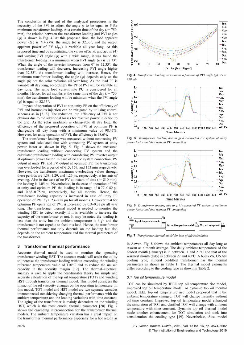
The conclusion at the end of the analytical procedures is thenecessity of the PVI to adjust the angle φ to be equal to θ forminimum transformer loading. At a certain time of the day (t = 750 min), the relation between the transformer loading and PVI angles(φ) is shown in Fig. 4. At this proposed time, the load apparentpower (SL) is 714 kVA, the angle (θ) is 32.33°, and the outputapparent power of PV (SPV) is variable all year long. At thisproposed time and by substituting the values of SL, θ, and SPV in (4)and varying PVI angle (φ) with a wide range, it was found thetransformer loading is a minimum when PVI angle (φ) is 32.33°.When the angle of the inverter increases from 0° to 32.33°, thetransformer loading will decrease. Increasing PVI angle higherthan 32.33°, the transformer loading will increase. Hence, forminimum transformer loading, the angle (φ) depends only on theangle (θ) not the solar radiation all year long. As the load PF isvariable all day long, accordingly the PF of PVI will be variable allday long. The same load current into PU is considered for allmonths. Hence, for all months at the same time of the day (t = 750 min), the transformer loading will be minimum when the PVI angle(φ) is equal to 32.33°.

Impact of operation of PVI at non-unity PF on the efficiency ofPVI and harmonics injection can be mitigated by utilising controlschemes as in [5, 8]. The reduction into efficiency of PVI is notobvious due to the additional losses for reactive power injection tothe grid. As the solar irradiance is changeable all day long, theefficiency of the proposed operation of PVI at optimum PF ischangeable all day long with a minimum value of 98.45%.However, for unity operation of PVI, the efficiency is 98.6%.

The transformer loading was measured without connecting PVsystem and calculated that with connecting PV system at unitypower factor as shown in Fig. 5. Fig. 6 shows the measuredtransformer loading without connecting PV system and thecalculated transformer loading with considering PV inverter outputat optimum power factor. In case of no PV system connection, PVoutput at unity PF, and PV output at optimum PF, the transformerwas overloaded for a period of 615, 167, and 153 min respectively.However, the transformer maximum overloading values throughthese periods are 1.38, 1.29, and 1.26 pu, respectively, at instants ofevening. Also in the case of no PV at instant of time (t = 810 min),the loading is 1.05 pu. Nevertheless, in the case of operation of PVIat unity and optimum PF, the loading is in range of 0.77–0.82 puand 0.68–0.75 pu, respectively, for all months. Hence, thetransformer loading capacity is increased in case of unity PFoperation of PVI by 0.23–0.28 pu for all months. However that foroptimum PF operation of PVI is increased by 0.3–0.37 pu all yearlong. The transformer thermal model is needed to monitor thewinding HST to detect exactly if it is available to increase thecapacity of the transformer or not. It may be noted the loading isless than the unity but the ambient temperature is high and thetransformer is not capable to feed this load. Hence, the transformerthermal performance not only depends on the loading but alsodepends on the ambient temperature and the thermal parameters ofthe transformer.

3 Transformer thermal performanceAccurate thermal model is used to monitor the operatingtransformer winding HST. The accurate model will assist the utilityto increase the transformer loading without exceeding the windingreference temperature value of 110°C and to reduce the unusedcapacity in the security margin [19]. The thermal–electricalanalogy is used to apply the heat-transfer theory for simple andaccurate calculation of the top oil temperature (TOT) and windingHST through transformer thermal model. This model considers theimpact of the oil viscosity changes on the operating temperature. Inthis model, TOT model and HST model are two separate cascadesinterconnected considering changing thermal performance with theambient temperature and the loading variations with time constant.The aging of the transformer is mainly dependent on the windingHST, which is the most crucial thermal parameter [20]. Fig. 7shows the cascading interconnection for the transformer thermalmodels. The ambient temperature variation has a great impact onthe transformer thermal performance especially for a hot region as

in Aswan. Fig. 8 shows the ambient temperatures all day long atAswan as a month average. The daily ambient temperature of thecoldest month (January) is in between 11 and 21°C and that of thewarmest month (July) is between 27 and 40°C. A 630 kVA, ONANcooling type, mineral oil-filled transformer has the thermalparameters as shown in Table 1. The thermal model exponentsdiffer according to the cooling type as shown in Table 2.

3.1 Top oil temperature model

TOT can be simulated by IEEE top oil temperature rise model,improved top oil temperature model, or dynamic top oil thermalmodel. IEEE top oil temperature rise model proposed that if theambient temperature changed, TOT will change instantly withoutoil time constant. Improved top oil temperature model enhancedthe simulation of TOT and clarified TOT will change with ambienttemperature with time constant. Dynamic top oil thermal modelmade another enhancement for TOT simulation and took intoconsideration the cooling type [19]. Nevertheless, Susa model

Fig. 4 Transformer loading variation as a function of PVI angle (φ) at t = 750 min

Fig. 5 Transformer loading due to grid connected PV system at unitypower factor and that without PV connection

Fig. 6 Transformer loading due to grid connected PV system at optimumpower factor and that without PV connection

Fig. 7 Transformer thermal model for loss of life calculation

3576 IET Gener. Transm. Distrib., 2019, Vol. 13 Iss. 16, pp. 3574-3582© The Institution of Engineering and Technology 2019

computes the transformer TOT considering the oil viscositychanges with the temperature. The increase in the transformerloading or the ambient temperature will lead to increasing TOTwith time constant [20]. Fig. 9 shows the transformer top oiltemperature model block diagram. The top oil temperature modelis formulated as [22]

1 + RxK2

1 + R xμpun xΔθoil, rated = μpu

n xτoil, ratedxdθoildt + θoil − θamb

1 + n

Δθoil, ratedn

(7)

τoil, rated = Cth − oil, ratedΔθoil, ratedqtot, rated

× 60 (8)

where Δθoil, rated is top-oil temperature under rated conditions riseover ambient (°C), θoil is operating temperature of the top-oil (°C),θamb is ambient temperature (°C), τoil, rated is time constant of oilunder rated conditions (minutes), K is the specified load attributionto rated load, qtot, rated is transformer total losses under ratedconditions (watt), R is attribution of rated load losses to no-load

losses, μpu is per-unit oil viscosity, Cth − oil, rated is oil thermalcapacitance under rated conditions (J/°C) and n is the coolingconstant for air moving fluid

The transformer oil thermal capacitance with external cooling isformulated as [20]

Cth − oil = Ywdn × mwdn × cwdn + Yfe × mfe × cfe + Yst × mmp × cmp

+Ooil × moil × coil(9)

where Ywdn is attribution of the winding losses to the total, losses ofthe transformer, Yfe is attribution of the core losses to the totallosses of the transformer, Yst is attribution of the stray losses to thetotal losses of the transformer, mwdn is winding material weight(kg), mfe is core weight (kg), mmp is tank and fittings weight (kg),moil is the oil weight (kg), cwdn is winding material specific heatcapacity (cCu = 0.11 and cAl = 0.25 Wh/kg°C ), cfe is core specificheat capacity, (cfe = 0.13 Wh/kg°C ), cmp is tank and fittingspecific heat capacity, (cmp = 0.13 Wh/kg°C ), coil is the oil specificheat capacity, (coil = 0.51 Wh/kg°C ) and Ooil is the oil correctionfactor for the ONAF and OFAF cooling modes,(Ooil = 0.86 Wh/kg°C ),

The transformer oil thermal capacitance without externalcooling is formulated as [21]

Cth − oil = mwdn × cwdn + mfe × cfe + mmp × cmp + moil × coil (10)

Equation (7) is used to simulate TOT variations all day long fordifferent scenario of PVI operation. Fig. 10 shows TOT variationsall day long as an average for each month without connecting PVsystem. At a certain time of the day (t = 810 min), TOT for allmonths is in between 74.8 and 90.1°C. In case of PV system outputat unity PF, TOT for all months is in between 59.5 and 74.2°C asshown in Fig. 11. If PVI operates at optimum PF, TOT is inbetween 55.7 and 70.5°C for all months as shown in Fig. 12.

3.2 Winding hot spot temperature model

The winding temperature distribution is not homogenous and thehottest portion represents the winding hot spot temperature, which

Fig. 8 Ambient temperatures all day long at Aswan as a month average

Table 1 Thermal parameters of 630 kVA mineral oil-filledtransformerTransformer parameters Value(I2R) rated windings losses 9023 WPEC − R (rated windings eddy current losses) 665 WPOSL − R (other stray losses under rated conditions) 1350 Wno load loss 1195 WPU eddy current losses at the hot spot location 0.72ratio of rated load losses to no load losses 9.24rated top oil rise 47.9°Crated hot spot rise 23°Cexponent n 0.25exponent n′ 0.25

Table 2 Thermal model exponents for cooling types [21]Cooling types n′ nno external cooling 0.25 0.25with external cooling 2 0.5

Fig. 9 Block diagram of the top oil temperature model

Fig. 10 TOT without PV system

Fig. 11 TOT for PV output power at unity power factor


3577

can damage the entire transformer or reduce its lifetime. Hence, itis the most crucial thermal parameter to determine the loadingcapability [23]. HST can be simulated by IEEE hot spottemperature rise model or dynamic hot spot thermal model. IEEEhot spot temperature rise model proposed that the winding HSTwill vary instantly with TOT without winding time constant.Dynamic hot spot thermal model took into consideration thecooling type for the simulation of HST [19]. However, Susa modelconsidered the oil viscosity impact on the calculation of HST. Theblock diagram of HST model is shown in Fig. 13. The windingHST model is given as [22]

K2 × Kθ + PEC − R puKθ

× μpun × Δθhs, rated = μpu

n × τwdg, rated × dθhsdt

+ θhs − θoil1 + n′

Δθhs, ratedn′

(11)

Kθ = θK + θhsθK + θavg

(12)

where PEC − R pu is pu winding eddy current losses under rated loadand at hot spot location, Δθhs, rated is hot spot temperature underrated conditions rise over top oil temperature (°C), θhs is operatingtemperature of winding hot spot (°C), τwdg, rated is time constant ofwinding under rated conditions (minutes), n′is cooling constant foroil moving fluid, Kθ is resistance correction because of temperature

change, θK is temperature factor for the loss correction, θavg isaverage winding temperature under rated load, θK = 235 forcopper, θK = 225 for aluminium.

Equation (11) is used to simulate the winding HST in case of noPV system, PVI operation at unity PF, and optimum PF as shownin Figs. 14, 15 and Fig. 16, respectively. Fig. 17 shows HST atinstant time (t = 810 min) for all months for the three cases. HST isin range between 117.1 and 130.2°C in case of no PV. Whenconnecting PV system at unity PF to feed the power to the loads inconjunction with the utility, the winding HST reduced by 30.5°C incomparison with no PV. N in case of PVI operation at optimum PF,the winding HST is reduced by 38.5°C compared to NO PV systemcase.

4 Transformer agingThe preservation of the lifetime of the transformer plays a crucialrole for the reliability of the power system. During the periods ofthe transformer overloading, the loss of life of the transformerincreases as the winding HST exceeds the reference temperaturevalue of 110°C. Aging acceleration factor (FAA) is an indicationfactor for the aging of the transformer, which can be modelled as in(13). Through certain period of time dt, the loss of life (Lf) can beexpressed as in (15) [23]

FAA = e 15, 000/383 − 15, 000/θH + 273 (13)

Fig. 12 TOT for PV output power at optimum power factor

Fig. 13 Block diagram of the hot spot temperature model

Fig. 14 HST without PV system

Fig. 15 HST for PV output power at unity power factor

Fig. 16 HST for PV output power at optimum power factor

Fig. 17 HST for PV output power at instant time (t = 810 min) in case ofwithout connecting PV system, PV inverter at unity PF, and PV inverter atoptimum PF


dL = FAAdt (14)

L f = 1T ∫

0

TFAAdt (15)

L f % = Accumulative age hours ∗ 100180, 000 (16)

From (13), if the winding HST is increased by 6.9°C, thetransformer will lose half of its life as the aging acceleration factorwill be doubled. Equation (16) is used to simulate the transformerloss of life for the three cases. The simulation of no PV systemshows the daily loss of life percent is fluctuating from 0.0295 to0.0887% according to the climatic and irradiance characteristics ofeach month as shown in Fig. 18. The sharpness of the loss of lifecurves in between 930 and 1000 min is due to the peak of thetransformer loading and the ambient temperature at this period.Fig. 19 shows the daily loss of life has been reduced to be inbetween 0.0054 and 0.0157% for case of injection active poweronly from PV system. Fig. 20 shows the PV system injection atoptimum power factor to the loads has been kept more reduction inthe loss of life to be in between 0.0039 to 0.0121%. This meansPVI operation at optimum PF has a great impact on the aging of thetransformer.

5 Economic and environmental assessmentThe economical aspects are necessary for engineers to makedecisions involving the cost to choose one solution rather than

another one. The engineers have a crucial role in making decisionsbased on the assessment of the expected outcome of theprofitability analysis. Mathematical formulas are used foranalysing and evaluating the engineering design alternatives [24].The investment into the energy is in a continuous increase, so theenergy losses cost need to be minimised to keep more profit for theinvestors. The utility and transformers users require more cost-effective transformer for economic aspects [25]. In this paper, theimpact of connecting PV system at unity and non-unity powerfactor on the transformer cost-effectiveness is investigatedreferring to the case of no connected PV system. The bid price ofthe transformer is the same for the different cases of PVI operation,but the cost of transformer energy losses are dependent on theloading conditions. The considered loading conditions are functionof the transformer thermal parameters, loading current, and theambient temperature. The ambient temperature impact is based onthe long-term conditions, so the cost-effectiveness is considered foreach month. In [14], the load losses are expressed as shown in (18).The monthly energy losses are shown in Fig. 21. The current yearcost of total energy losses of the transformer is expressed bysumming the cost of the transformer energy losses for all months ofthe year as in (17). The monthly energy losses into the transformerare obtained by multiplying the daily energy losses into thetransformer by the day per month and by the energy tarrif (LE/kWh). The daily energy losses (kWh) are obtained by integratingthe total losses into the transformer (kW) all day long

CTL = ∑i = 1

12DPMi × ET × ∫

0

TNLL + LL × Ki

2 dt (17)

LL = P × Kθ + PEC − RKθ

+ POSL (18)

where CTL is the annual cost (LE/year) of the transformer energylosses, NLL is no-load losses (kW), LL is rated load losses (kW),Ki

2 is the square of the specified load attribution to rated load formonth i, P is ohmic losses (kW), PEC − R is rated eddy currentlosses (kW), POSL is other stray losses (kW), ET is energy tariff(LE/kWh), DPMi is days per month i (day), and i indicates themonth.

The Egyptian average energy tariff is 1.05 LE/kWh. Thepayback period of the PV system can be obtained by dividing thetotal PV system cost by the saving of the consumed energy andenergy losses costs. If the transformer particular rises with lowlosses, this will reduce the payback period. If the PVI operation ledto more saving into the energy losses and the consumed energy,this will lead to more profit and low amortisation period. Also, theGHG due to combustion of fossil fuel for generation plants will bereduced. GHG emission can cost the authority to raise the healthcare. Hence, this cost is called environmental cost. When using thePF-controlled PVI through grid connection to minimise thetransformer losses, the environmental cost is minimised.

For the environment protection, some countries set limit for theGHG emissions and the associations or utilities exceed this limitneed to pay penalty or purchase GHG credits from other that havesurplus of GHG credits. Hence, the environmental cost is includedin the evaluation of the cost-effectiveness of the transformer. Toevaluate the environmental cost due to the transformer energylosses, it is necessary to calculate the cost factor (LE/MWh) of thecurrent year GHG emissions as follows: [26]

C = Cy ∑j = 1

Nf j × ej (19)

ej = eCO2, j + 21eCH4, j + 310eN2O, j0.0036

nj 1 − λj(20)

where Cy is cost of the current year GHG emissions (900 LE/tCO2),tCO2 is equivalent tonnes of CO2 emissions, j is fuel type, N is fuelsnumber of electricity mixture, fj is the percent of the consuming

Fig. 18 Daily loss of life percentage as an average for the month withoutPV system

Fig. 19 Daily loss of life percentage as an average for the month for PVoutput power at unity power factor

Fig. 20 Daily loss of life percentage as an average for the month for PVoutput power at optimum power factor


3579

electricity coming from fuel j, ej is the emission factor of fuel j(tCO2/MWh), eCO2, j is emission factor of CO2 for fuel j (kg/GJ),eCH4, j is emission factor of CH4 for fuel j (kg/GJ), eN2O, j is emissionfactor of N2O for fuel j (kg/GJ), λj is percent of energy lost in thegrid for fuel j, and nj is the conversion efficiency for fuel j (%)

To investigate the difference of the PVI operation impact on theenvironmental cost, the environmental parameters in [26] areconsidered. The considered emission GHGs are methane (CH4),carbon dioxide (CO2), and nitrous oxide (NO2). Table 3 shows theconsidered fuel types. To determine GHG emissions due totransformer energy losses, the emission factor will be multiplied bythe transformer energy losses.

The environmental cost is expressed by summing the monthlyenvironmental cost due to the transformer energy losses as in (21).The monthly environmental cost due to the transformer energylosses is obtained by multiplying the day per month by the daily

energy losses into the transformer and by the cost factor (LE/MWh) of the current year GHG emissions and by 0.001 to convertthe cost factor to (LE/kWh). Also, the saving into theenvironmental cost due to the difference of the operation of PVIreferring to the case of no PV is expressed by subtracting theannual cost of the environmental impact (LE/year) in case ofoperation of PVI at unity or optimum PF from that without PV asin (22)

EC = ∑i = 1

12DPMi × C × 10−3 × ∫

0

TNLL + LL × Ki

2 dt (21)

SEC = ∑i = 1

12DPMi × C × LL × 10−3 × ∫

0

TΔKi

2 dt (22)

where EC is the annual cost of the environmental impact (LE/year),SEC is saving into the annual cost of the environmental impact(LE/year), ΔKi

2 is difference between the square of loading formonth i.

The simulations show the annual energy losses of thetransformer in case of unity PF of PVI is less than that without PVconnection. However, in case of optimum PF of PVI, the energylosses are the minimum of the three scenarios as shown in Table 4.Hence, in case of optimum PF of PVI, the cost of the annual energylosses are the minimum. Also, the equivalent tonnes of CO2emissions are minimum due to the transformer energy losses areminimum and its environmental cost is the minimum. Fig. 22shows a comparison chart of the equivalent tonnes of CO2emissions in case of without connecting PV system, PVI at unityPF, and PVI at optimum PF. The saving into the annual cost of theenvironmental impact is referring to the case of no PV. As well, theminimisation of the transformer energy losses is an indication forminimum amortisation period of the PV system. The paybackperiod of PV system in case of unity PF of PVI is 11.3 year.Nevertheless that for optimum PF of PVI is 10.4 year referring tothe case of no PV.

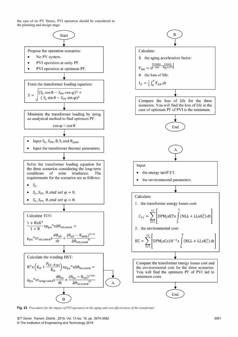
Now, the procedures of how to study the impact of PVIoperation on the aging and cost-effectiveness of the transformer,the GHGs emissions, and the environmental cost are shown inFig. 23.

6 ConclusionsThe objective of this paper is to show the impact of PV power-factor-controlled inverter on the transformer loss of life, cost-effectiveness, GHG emissions, and environmental cost consideringlong-term characteristics of ambient temperatures and solarirradiance. It has been shown that the grid power factor is reducedwhen operating PVI at unity PF. However operating it at non-unityPF, this led to the improvement into the grid PF. A proposedanalytical method is used to find the optimum PF of PVI tominimise the transformer loading. The transformer loading wasmeasured in case of no PV system connection to the loads and wascalculated in case of PVI operation at unity PF and optimum PF.These three scenarios of transformer loading are used to evaluatethe impact of PVI operation. The considered transformer is 630 kVA, ONAN cooling type, and mineral oil. The top oil temperatureand the winding hottest spot temperature are simulated for the threecases. The results show the operation of PVI to inject only activepower leads to reducing HST by 30.5°C at time (t = 810 min)referring to no PV case. However the optimum PF of PVI leads todecreasing HST by 38.5°C at the same instant of time comparedwith no PV scenario. Also, the optimum PF minimised the dailyloss of life to be in between 0.0039 and 0.0121% respecting to allmonths. The transformer energy losses are the minimum inbetween the three cases due to operating of PVI at optimum anglebetween the voltage and the current of the inverter. Theminimisation of transformer energy losses led to minimising theGHGs emissions and also the environmental cost. Also, thepayback period of PV system in case of unity PF of PVI is 11.3year. However that for optimum PF of PVI is 10.4 year referring to

Fig. 21 Monthly energy losses for case of without connecting PV system,PVI at unity PF, and PVI at optimum PF

Table 3 GHG emissions of fossil fuel plantsFuel type Natural gas Diesel Coalf j, % 15 7.6 69.77eCO2, j, kg/GJ 56.1 74.1 94.6

eCH4, j, kg/GJ 0.003 0.002 0.002

eN2O, j, kg/GJ 0.001 0.002 0.003

λj, % 8 8 8nj, % 45 30 35

Table 4 Annual energy losses, its cost, and its impact onthe environmental costPVI status WO PV Unity PF of PVI Optimum PF of

PVIannual energylosses, kWh

107,814 86,118 82,390

CTL, LE/year 113,204.7 90,423.9 86,509.5EC, LE/year 86,669.52 69,228.54 66,231.67SEC, LE/year — 17,440.98 20,437.85tCO2 96.3 76.92 73.59

Fig. 22 GHG emissions chart in case of without connecting PV system,PVI at unity PF, and PVI at optimum PF


the case of no PV. Hence, PVI operation should be considered inthe planning and design stage.

Fig. 23 Procedures for the impact of PVI operation on the aging and cost-effectiveness of the transformer


3581

7 References[1] Sehar, F., Pipattanasomporn, M., Rahman, S.: ‘An energy management model

to study energy and peak power savings from PV and storage in demandresponsive buildings’, Appl. Energy J., 2016, 173, pp. 406–417

[2] Hartner, M., Mayr, D., Kollmann, A., et al.: ‘Optimal sizing of residential PV-systems from a household and social cost perspective – a case study inAustria’, Sol. Energy J., 2017, 141, pp. 49–58

[3] Karimi, M., Mokhlis, H., Naidu, K., et al.: ‘Photovoltaic penetration issuesand impacts in distribution network – a review’, Renew. Sustain. Energy Rev.J., 2016, 53, pp. 594–605

[4] Peng, W., Baghzouz, Y., Haddad, S.: ‘Local load power factor correction bygrid-interactive PV inverters’. 2013 IEEE Grenoble Conf., Grenoble, France,June 2013, pp. 1–6

[5] Yang, Y., Blaabjerg, F., Wang, H.: ‘Low voltage ride-through of single-phasetransformerless photovoltaic inverters’, IEEE Trans. Ind. Appl., 2014, 50, pp.1942–1952

[6] Brandao, D.I., Mendes, F.E.G., Ferreira, R.V., et al.: ‘Active and reactivepower injection strategies for three-phase four-wire inverters duringsymmetrical/asymmetrical voltage sags’, IEEE Trans. Ind. Appl., 2019, 1, pp.1–8

[7] Park, S., Kwon, M., Choi, S.: ‘Reactive power P&O anti-islanding method forgrid connected inverter with critical load’, IEEE Trans. Power Electron.,2018, 34, pp. 204–212

[8] Miret, J., Camacho, A., Castilla, M., et al.: ‘Control scheme with voltagesupport capability for distributed generation inverters under voltage sags’,IEEE Trans. Power Electron., 2013, 28, pp. 5252–5262

[9] El Batawy, S.A., Morsi, W.G.: ‘Optimal secondary distribution system designconsidering rooftop solar photovoltaics’, IEEE Trans. Sustain. Energy J.,2016, 7, pp. 1662–1671

[10] Vu, P., Nguyen, Q., Tran, M., et al.: ‘Adaptive backstepping approach for dc-side controllers of Z-source inverters in grid-tied PV system applications’,IET Power Electron., 2018, 11, pp. 2346–2354

[11] Ma, L., Xu, H., Huang, A.Q., et al.: ‘Single-phase hybrid-H6 transformerlessPV grid-tied inverter’, IET Power Electron., 2018, 11, pp. 2440–2449

[12] Eltawil, M.A., Zhao, Z.: ‘Grid-connected photovoltaic power systems:technical and potential problems – a review’, Renew. Sust. Energy Rev., 2010,14, pp. 112–129

[13] Camacho, A., Castilla, M., Miret, J., et al.: ‘Flexible voltage support controlfor three-phase distributed generation inverters under grid fault’, IEEE Trans.Ind. Electron., 2013, 60, pp. 1429–1441

[14] Salama, M.M.M., Mansour, D.-E.A., Abdelkasoud, S.M., et al.: ‘Impact oflong-term climatic conditions on the ageing and cost-effectiveness of the oil-filled transformer’. 2018 Twentieth Int. Middle East Power Systems Conf.(MEPCON), Cairo, Egypt, 18–20 December 2018, pp. 494–499

[15] Emara, M.M., Mansour, D.A., Azmy, A.M.: ‘Mitigating the impact of agingbyproducts in transformer oil using TiO2 nanofillers’, IEEE Trans. Dielectr.Electr. Insul., 2017, 24, pp. 3471–3480

[16] Sreekanth, T., Lakshminarasamma, N., Mishra, M.K.: ‘Grid tied single-stageinverter for low-voltage PV systems with reactive power control’, IET PowerElectron., 2018, 11, pp. 1766–1773

[17] https://sam.nrel.gov/weather, Monday, 3–9-2018, 11:00 am[18] Serovajsky, S.: ‘Optimization and differentiation’ (CRC Press, Boca Raton,

FL, USA, 2018)[19] Abbas, A., Elzahab, E.A., Elbendary, A.: ‘Thermal modeling and ageing of

transformer under harmonic currents’. 23rd Int. Conf. on ElectricityDistribution, Lyon, France, 15–18 June 2015, pp. 1–5

[20] Susa, D., Nordman, H.: ‘A simple model for calculating transformer hot-spottemperature’, IEEE Trans. Power Deliv., 2009, 24, pp. 1257–1265

[21] Susa, D., Lehtonen, M.: ‘Dynamic thermal modeling of power transformers:further development – part I’, IEEE Trans. Power Deliv., 2006, 21, pp. 1961–1970

[22] Cui, Y., Ma, H., Saha, T., et al.: ‘Moisture-dependent thermal modelling ofpower transformer’, IEEE Trans. Power Deliv., 2016, 31, pp. 2140–2150

[23] Paterakis, N.G., Pappi, I.N., Erdinç, O., et al.: ‘Consideration of the impactsof a smart neighborhood load on transformer aging’, IEEE Trans. Smart Grid,2016, 7, pp. 2793–2802

[24] Blank, L., Tarquin, A.: ‘Engineering economy’ (New York, USA, 2018, 8thedn.)

[25] Charalambous, C.A., Milidonis, A., Lazari, A., et al.: ‘Loss evaluation andtotal ownership cost of power transformers – part I: a comprehensivemethod’, IEEE Trans. Power Deliv., 2013, 28, pp. 1872–1880

[26] Georgilakis, P.S., Amoiralis, E.I.: ‘Distribution transformer cost evaluationmethodology incorporating environmental cost’, IET Gener. Transm. Distrib.,2010, 4, pp. 861–872


https://sam.nrel.gov/weather

research article considering long-term characteristics iet

Documents