Research Article focuses on the analysis and resolution of managerial issues based on analytical and empirical studies.

Linkage between Economic Value Added and Market Value: An Analysis

Ashok Banerjee Introduction

Maximizing shareholder value has become the new corporate paradigm. Corporations in the US have started disclosing EVA information from the beginning of 90s as a measure of corporate performance. It is believed that market value of a firm (hence shareholder wealth) would increase with the increase in EVA. Various studies done in the US also confirm this belief. EVA (a term coined and registered by Stern Stewart & Co. New York) is a residual income that subtracts the cost of capital from the operating profits generated by a business. The present study makes an at tempt to find the relevance of Stewart's claim that market value of the firm is largely driven by its EVA generating capacity in the Indian context. Based on a sample of 200 firms over a period of five years, the study shows that market value of a firm can be well predicted by estimated future EVA streams. The study has also found that market value of most of the firms in the sample is explained more by current operational value than future growth value of firms.

Ashok Banerjee is Associate Professor in the Accounting and Finance Area of the Indian Institute of Management, Lucknow.

Maximizing shareholder value has become the new corporate paradigm. Although shareholder wealth maximization has traditionally been recognized by managers and researchers as the ultimate corporate goal, the maxim has gained new dimension in recent years, thanks to the concept of Economic Value Added (EVA) coined and registered by Stern Stewart & Co, New York. EVA is a residual income that subtracts the cost of capital from the operating profits generated by a business. Corporations in the US started disclosing EVA information from the begin-ning of 90s. Since then, the number of companies adopting EVA has increased (Wallace, 1997). More than 300 companies, with revenue approaching a trillion dollars a year, have implemented EVA framework for financial management and incentive compensation (Ehrbar, 1998). Adopting EVA philo-sophy forces a company to find ingenious ways to do more with less capital (Tully, 1993).

This does not mean EVA concept retards growth. It only suggests that so long as a company is earning a return on its investment in excess of the cost of investment, there is no limit to growth. It is only when the earning is insufficient to meet the cost of funds tied up, there arises a need to unlock the fund and thereby avoid or minimize bad or uneconomic investments. EVA is a modified version of share-holder value theory. The shareholder value theory places shareholders at the top in analysing the economic performance of a business. The share-holder value approach (Rappaport, 1986) estimates the economic value of an investment by discounting forecasted cash flows by the cost of capital. These cash flows, in turn, serve as the foundation for shareholder returns from dividend and share price appreciation. EVA is different from shareholder value theory in the sense that it deducts depreciation to compute its residual income and also it makes certain adjustments to convert accounting profit to economic profit. It is believed that market value of a firm, at any given moment, is the summation of

Vol. 25, No. 3, July-September 2000 23 Vikalpa

beginning invested capital and present value of future stream of expected EVAs. Stewart (1991) emphasized that to get significant benefits, EVA should be fully integrated into a company linking executive compensation to improvement in EVA. Stewart maintained that if executives' bonus and other incentives were linked to traditional para-meters [e.g., Earnings per share (EPS), turnover, Return on Net Worth (RONW), etc.], EVA would fail as a performance measure. This is because corporate executives, in that case, would have no incentive to maximize EVA. EVA, thus, is not merely a financial computation reported at the end of the year but is a part of the fully integrated management system. Implementation of EVA system in an or-ganization takes a long time as EVA does not mean only laying down measurement or computational techniques. Stewart mentions in Ehrbar (1998) that there are four Ms in the implementation process — Measurement, Management System, Motivation, and Mindset. Thus, Stewart (1991) argues that market value of a firm is largely driven by its EVA generating capacity. The present study makes an attempt to find the relevance of Stewart's claim in the Indian context. The relationship between EVA and market value is tested on a sample of 200 companies. The results of the study confirm Stewart's claim.

It is believed that EVA is a better performance measure than traditional measures like Earning per Share (EPS), Return on Capital Employed (ROCE), or Return on Net Worth (RONW). EPS depends largely on the vagaries of accounting policies fol-lowed by a firm. Thus, EPS is as much reliable as the accounting profit. Accounting profit (PAT) de-pends, inter alia, on the firm's capital structure. A lowly geared firm would return a higher PAT than a highly geared firm, given the same level of operating profit earned by both the firms. In computing accounting profit, only one part of cost of capital (i.e., borrowing cost) is deducted. As a result, PAT does not reflect the true economic profit. EVA, on the other hand, is the residual profit after deducting full cost of capital from operating profits. ROCE or RONW considers only one side of the performance. Exclusive reliance on ROCE or RONW may lead to rejection of economically profitable projects or acceptance of unviable projects. Both would lead to destruction of shareholder value. Consider a firm with a present ROCE of 22 per cent and an overall cost of capital of 18 per cent. The firm receives a new investment proposal with an estimated ROCE of 20 per cent, cost of capital remaining unchanged. If the firm's objective is to

maximize ROCE, it may reject the project. But, actually, the project would have added two per cent economic surplus to the wealth of the firm. Consider another example. Suppose the present ROCE of the firm is ten per cent and cost of capital 16 per cent. The firm receives a new investment proposal with an estimated ROCE of 12 per cent, with no change in cost of capital. The firm would accept the proposal to maximize ROCE. But this decision would destroy the firm's wealth. EVA compares ROCE with the cost of invested capital and a firm, with the objective of EVA maximization, would accept all fresh invest-ment proposals so long as the expected spread is positive.

Definition of EVA

EVA essentially seeks to measure a company's actual rate of return as against the required rate of return. To put it simply, EVA is the difference between Net Operating Profit after Tax (NOPAT) and the capital charge for both debt and equity (overall cost of capital). If NOPAT exceeds the capital charge, EVA is positive and if NOPAT is less than capital charge, EVA is negative.

The definition of EVA can be mathematically shown as below:

EVA = NOPAT- Capital Charge ............. ( Eq. 1) = NOPAT- (WACC * Invested Capital) = (r * Invested Capital)-(c * Invested Capital)

EVA = (r-c) * Invested Capital EVAt = (r-c) * Invested Capital (M) ................... (Eq.2) Where, WACC = Weighted Average Cost of

Capital Invested Capital = Invested Capital at the

Beginning of the Year r = NOPAT/Invested Capital c = WACC t = Time Period

The spread (r-c) shows whether a company has earned a return from its business that is more than its total cost of capital. If the spread is positive, EVA would also be positive. The logic for taking begin-ning invested capital for calculating periodic EVA is that a company would at least take a year's time to earn a return on investment. Given a particular level of spread, EVA would depend on the beginning invested capital. Given a particular level of invested

Vol. 25, No. 3, July-September 2000 24 Vikalpa

capital, EVA would depend on spread. Thus, there are two factors that drive EVA — the spread and the invested capital. The spread denotes the relative profitability and invested capital denotes the size or growth. If a company has negative profitability (i.e., spread), growth in size would reduce EVA. To reduce the impact of negative EVA, invested capital should be economized. On the other hand, if the spread is positive, growth in firm size would indicate higher EVA. However, it is true that for skill-based com-panies (e.g., companies in the Information Technol-ogy sector) growth does not involve commensurate increase in invested capital. This may prompt some people to conclude that EVA would not be a useful variable to explain stock price movements of a research-based or skill-driven company. But, Stewart (1991) defended EVA on this count. Thus, the message of the EVA formula (Eq. 2) is that if the return (r) of a company is not adequate enough to cover the cost of capital (c) in full, more investment in the business would mean more negative EVA. In such a situation, the company should try to either increase the 'r' or reduce the capital invested to improve EVA. The idea behind EVA is that share-holders must earn a return that compensates the risk taken. A zero EVA indicates that the return earned is just sufficient to compensate the risk. EVA holds a company accountable for the cost of capital it uses to expand and operate its business and attempts to show whether a company is creating real value for its shareholders.

Stewart (1991) defines NOPAT as the "profits derived from the company's operations after taxes but before financing costs and non-cash-book keep-ing entries." But, in eliminating the impact of "non-cash-book keeping" entries, Stewart makes an ex-ception. Depreciation is subtracted to arrive at NOPAT. Stewart argues that depreciation is sub-tracted because it is "a true economic expense." In other words, NOPAT is equivalent to income avail-able to shareholders plus interest expenses (after tax). It may be noted that Stewart has considered regular non-operating income (e.g., interest/dividend on investment) as part of NOPAT. This is a deviation from traditional definition of operating profit. Also, to compute NOPAT properly, Stewart identified 120 adjustments (Ehrbar, 1998) to be made to accounting profit as reported in the profit and loss account. These adjustments, it is argued, would eliminate potential distortions in accounting results based on Generally Accepted Accounting Principles (GAAP) of a country.

However, the actual number of adjustments would depend on prevailing GAAP of a country. In order to avoid complexity in the calculation of NOPAT, Stewart (1991) suggested four common adjustments to be made — Adjustments for Deferred Tax Reserve, Last-in-First-Out (LIFO) Reserve, Goodwill Amortization and R&D Cost Amortization. These items are called Equity Equivalents.* Equity Equivalents are added to invested capital and periodic change is taken to NOPAT. These adjustments make NOPAT a realistic measure of yield generated for investors for recurring business activities. It is believed that these adjustments would truly convert accounting profit to economic profit.

However, for the purpose of this study, the computation of NOPAT has been further modified. NOPAT has been defined as below:

NOPAT = PBIT (nnrt) * (1-T)

Where, PBIT (nnrt) = Profit Before Interest and Taxes (net of non-recur-ring transactions)

= Profit After Tax (PAT)+ Provision for Tax + Inter-est Expense + Lease Rent-Extraordinary Income+ Extraordinary Expenses.

T = Effective Tax Rate (Provision for Tax/PBT).

Invested capital refers to total assets (net of revaluation) net of non-interest bearing liabilities. From an operating perspective, invested capital can be defined as Net Fixed Assets (i.e. net block), plus investments plus Net Current Assets. Net Current Assets denote current assets net of Non-Interest-Bearing Current Liabilities (NIBCLS). From a financ-ing perspective, the same can be defined as Net Worth plus total borrowings. Total borrowings denote all interest bearing debts. Stewart (1991) mentioned that adjustments for four Equity Equivalents men-tioned above should be made. The adjustments for Equity Equivalents are intended to arrive at the economic value of invested capital. Equity Equiva-lents eliminate accounting distortions. Net worth is defined as paid up share capital plus reserves and surplus (net of revaluation reserves) less miscellane-ous expenditure less accumulated losses, if any. One

'For a detailed discussion on Equity Equivalents and their treatment, interested readers may refer to Stewart, B III (1991), The Quest for Value, Harper Business Publications.

Vol. 25, No. 3, July-September 2000 25 Vikalpa

may argue that this method of calculating invested capital is not free from depreciation distortions. Since net block of depreciable assets is considered, different corporate depreciation policy would affect the invested capital and hence EVA. Stewart (1991) tackles it by prescribing a uniform method of charging depreciation. He mentions that a straight-line depreciation or annuity method of depreciation would minimize the distortions. Such adjusted in-vested capital (after adjusting for Equity Equivalents and depreciation) would be called economic capital. However, invested capital for the purpose of the study is defined as follows:

Invested Capital = Net Worth + Total Borrowings

Where, Net Worth = Share Capital + Reserves and Surplus - Revaluation Re-serve-Accumulated Losses -Miscellaneous Expenditure

Total Borrowings = Long-term Interest-bearing Debt + Short-term Interest-bearing Debt

Adjustments for Equity Equivalents are not considered in the present study because these are largely non-existent or inapplicable in Indian con-ditions (Banerjee, 1999).

Thus, the computational methodology of EVA is not unique. Ehrbar (1998) talked about an EVA spectrum. At one extreme is what is called "Basic EVA." This is a rudimentary form of EVA arrived at without making any adjustments. Then follows "Disclosed EVA." It is the EVA computed by Stern Stewart & Co to rank companies. "Disclosed EVA" is computed by making about "a dozen of standard adjustments to publicly available accounting data." Next is "Tailored EVA." An insider can calculate this EVA by making tailor-made adjustments peculiar to the organization concerned. At the other extreme of the spectrum is "True EVA."This is the theoreti-cally correct and accurate measure of EVA calculated with all relevant adjustments to accounting data and using the precise cost of capital of each division of an organization. It is extremely difficult to compute "True EVA."

Truly speaking, "Tailored EVA" is the ideal EVA measure. But, it is difficult for an outsider to use this definition of EVA for sheer lack of information. Therefore, in the present study, EVA has been calculated in a manner that lies in between "Basic EVA" and "Disclosed EVA." Having defined most of

the parameters in the computation of EVA, we now look at the last factor i.e., WACC.

WACC has been defined in the study to include three specific costs, viz., cost of equity shares, cost of preference shares, and cost of borrowings (debt).

Cost of Debt (Kd) is calculated -by multiplying the pre-tax debt cost with (1-t). It may be noted that 't' denotes the effective tax rate.

Cost of Preference Shares (Kp)= (Preference dividend/ Beginning preference share capital) * 100. Corporate dividend tax has not been considered because it was not in vogue during the period under study.

Cost of Equity (Ke) is an opportunity cost equal to the total return that an investor in a company's equity could expect to earn from alternative investments of comparable risk. Cost of equity is not an explicit cost like cost of debt. The dividend-based approach or earning-based approach of finding out cost of equity is not a valid way of calculating the return expected by equity shareholders. These approaches only measure the explicit cost of servicing equity. But, the true measure of equity cost is not what a company offers but what investors expect. The opportunity cost of equity capital has been calculated by following Capital Asset Pricing Model (CAPM)* (Sharpe, 1964).

EVA and Net Present Value (NPV)

It is widely tested that the value of a firm is given by the present value of future stream of free cash flows. Cash flow is the value driver. Of course, cash flow also depends on certain operating value drivers. The NPV method of measuring firm value is used by Rappaport (1986) in defining shareholder value of a firm. EVA proponents claim that the firm value can be measured by discounting future EVAs instead of future cash flows. A question may naturally arise - will the firm value differ under EVA and cash flow approaches? As Table 1 illustrates, the life-time value of the firm would be the same in the EVA method of valuation as in the NPV method. We take a simple

*CAPM recognizes the risks associated with equity instruments and proposes that an investor in this instrument would expect a risk premium over and above the risk-free rate of return prevailing in the market. Such a risk premium woutd depend on the volatility of returns of the equity scrip vis-a-vis that of market (usually represented by an index). Higher the volatility, greater would be the risk premium. According to CAPM, the expected return on equity (i.e., opportunity cost of equity capital) = Rf + P[E(RJ - R(], where f$ represents volatility, Rf the risk-free rate and E(Rm) the expected market return.

Vol. 25, No. 3, July-September 2000 26 Vikalpa

example to illustrate the similarity by considering a firm with a single line of business having five-year life and a cost of capital of 18 per cent (Table 1).

The critical issue, therefore, is: Why should we use EVA? EVA is better because it is an annual measure as well as a life-time measure. NPV only measures the life-time value of a firm. NPV or cash flow-based method cannot return a reliable annual performance measure. A firm with high growth potential would show negative annual cash flows in the years of growth due to heavy investments. NPV method deducts the entire investments made for future growth in one year and thereby reports a negative cash flow figure for high-growth firms. EVA, on the other hand, deducts only a capital charge on such investments from NOPAT. A dotcom firm, for example, would show huge negative cash flows in the first few years of its existence in spite of high revenue. But, the share price of the firm may still go up. In such a situation, the cash flow-based model may fail to explain the share price movements. Also, it may be difficult to project future cash flows on the basis of past negative cash flows. EVA measure would deduct a capital charge on massive investments made by the dotcom firm in initial years and hence would return a more reliable annual performance

figure. Thus, new economy firms may be better valued with EVA.

The advantage of EVA over cash flows' is also echoed by Sirower and O'Byrne (1998). They advocated the use of EVA in place of cash flows to measure periodic operating performance. They observed that the main shortcoming of free cash flow (FCF) as a measure of periodic operating perform-ance is that "it subtracts the entire cost of an investment in the year in which it occurs.... EVA effectively capitalizes instead of expensing such corporate investment, and then holds management accountable for that capital by assigning a capital charge."

EVA and Market Value Added: Relationship

EVA theory simply emphasizes that earning a return greater than the cost of capital increases the value of a company and earning less than the cost of capital decreases the value. Stewart (1991) has introduced another measure of shareholder value called Market Value Added (MVA). MVA tells us how much value the market adds over the book value of invested capital. MVA, therefore, denotes the confidence of

Table 1: A Comparison of NPV and EVA Methods

Period Invested Capital Operating Profit before Depreciation Depreciation NOPAT

0 200

1 75 90 15 2 120 49.5 70.5 3 130 27.23 102.77 4 145 14.97 130.03 5 (10.06)* 130 8.24 121.76

'Realizable value of assets at the end of five years.

NPV (Method) EVA (Method) Period Cash Flows PV o f Cash

Flows NOPAT Invested

Capital Cost of Capital

EVA PV of EVA

0 -200 -200

1 75 63.56 -15 200 36 -51 -43.22 2 120 86.18 70.5 110 19.8 50.7 36.41 3 130 79.12 102.77 60.5 10.89 91.88 55.92 4 145 74.79 130.03 33.27 5.99 124.04 63.98 5 140.06 61.22 121.76 18.30 3.29 118.47 51.78 Value of the Firm 164.87 164.87

Vol. 25, No. 3, July-September 2000 27 Vikalpa

considered as independent variables and MVA has been considered as dependent variables. The rela-tionship between independent and dependent var-iables was tested in nine industries over a period of six years (1992-93 to 1997-98). In addition to conducting regression analysis on each industry separately, the same analysis is carried on all companies across the nine chosen industries (cross-sectional analysis) for each year. The study failed to conclude convincingly about the superiority of EVA over other independent variables in explaining MVA. The study, however, singled out EVA as the common significant explanatory variable across industries. The study could only show that of the five independent variables, EVA is the better of the lot.

The objective of the present study is to examine whether the market value of a firm is best predicted by expected EVAs. In other words, Stewart's talked about relationship of market value as equivalent to the sum of present value of future stream of expected EVAs is examined. The market value of a firm is always futuristic. It captures information about a firm not yet operationally materialized and hence not present in its income statement. Explaining change in market value of a firm on the basis of one-year EVA value may not be quite correct. Stewart (1991) also mentions that MVA is the present value of future stream of EVAs. Stewart coined the term Market Value Added to measure shareholder wealth. MVA is defined as absolute rupee spread between a com-pany's market value and its invested capital. In other words, MVA is the difference between a company's market value of invested capital and book value of invested capital. The market value of debt is not readily available, as debts are mostly not traded. Therefore, the definition of MVA can be modified as below:

MVA = Market Capitalization - Equity Share Cap-ital + Reserves and Surplus - Revaluation Reserves-Accumulated Losses - Miscella-neous Expenditure.

................ (Eq-9) It can be observed from the above modified

definition that MVA is almost similar to market price-book value (p/b) ratio. The only difference is that MVA is an absolute measure and p/b ratio is a relative measure. If MVA is positive, it implies that p/b is greater than one. Negative MVA implies a less than one p/b ratio. Successful companies add their MVA and thus increase the value of capital invested in the business. It is argued that MVA

depends on the rate of return of a company. If a company's rate of return exceeds its cost of capital, the company will sell in the stock market with a premium compared to its book value of capital. On the other hand, companies that have rate of return smaller than their cost of capital will sell with discount compared to their book value of capital. This principle also applies to EVA. Thus, it is said that positive EVA also means positive MVA and vice versa (Stewart, 1991). Maximizing MVA, therefore, should be the primary objective for any company that is concerned about its shareholders' welfare. Thus, EVA is the internal measure of corporate performance and MVA is the external measure of corporate performance. MVA reflects how much the capital market is putting value on the invested capital.

Hence, market value is deemed to be predicted well with stream of future expected EVAs and not only with current year EVA. The sample size considered for the present study is 200 and the relationship between EVA and market value is tested over a five-year period data (1993-94 to 1997-98).

Previous Studies

The empirical research of academics to date on this subject is limited. The results of these studies are mixed. Stewart (1991) has first studied the relation-ship with market data of 618 US companies. Stewart observed that the relationship between EVA and MVA is highly correlated among US companies. Lehn and Makhija (1996) in their study of 241 US companies over two periods (1987-1988 and 1992-1993) observed that both measures (EVA and MVA) correlate positively with stock returns and that the correlation is slightly better with EVA than that with traditional performance measures like return on assets (ROA), return on equity (ROE), etc. On the predictive power of EVA in explaining MVA or shareholder wealth, several researchers (for example, Uyemura, Kantor and Petit, 1996; McCormack and Vytheeswaran, 1998; O'Byrne, 1996; Milunovich and Tsuei, 1996; Grant, 1996) observed that EVA is better correlated with MVA or shareholder wealth than other traditional parameters like ROCE, RONW, EPS, etc. However, there are adverse findings too. Dodd and Chen (1996) found that return on assets (ROA). explained stock returns better than EVA. Hamel (1997) was critical about the superiority of EVA. He opined that EVA reveals little about a company's share of new wealth creation.

Vol. 25, No. 3, July-September 2000 29 Vikalpa

Research Methodology

It has already been mentioned that:

Cost of Borrowings (KJ = (Total Interest Expense/ Beginning Total Borrowings) * (1-T) * 100

.............(Eq. 10)

It may so happen that Kd calculated according to Equation 10 may return an abnormally high figure. This is because the total interest expenses may be too high compared to the beginning total interest-bearing debts. This would give a distorted borrowing cost figure. The borrowing cost number can show an artificially high figure because of the following reasons: • Loans taken during the current year have been

repaid. Loans taken at the beginning of the current year so that it does not appear at the denominator of Kd calculation.

• Rescheduling of loan repayment. Hence, a control variable "normal yearly bor-

rowing cost" has been considered. This is taken as the Prime Lending Rate (PLR) of the concerned year of State Bank of India. The SBI's PLR for the period under study is shown in Table 2 (RBI, 1996-97, 1997-98).

If the computed Kd in any year is more than the control variable (after-tax), the after-tax control variable has been considered as the borrowing cost of that year. This has been done to see whether the borrowing cost represents the prevailing lending rates of the banks. If the computed Kd in any year is less than the control variable (after-tax), no adjustment is made to Kf This is to recognize the innovative financing routes followed by companies to minimize borrowing costs.

An earlier study on EVA (Banerjee, 1999) used daily stock returns to compute beta for the purpose

Table 2: SBI's Prime Lending Rate (PLR)

Year SBI's PLR(%)

1992-93 19.0 1993-94 19.0 1994-95 15.0 1995-96 16.5 1996-97 14.5 1997-98 14.0

of estimating cost of equity. Use of corporate beta on the basis of daily share prices may not be prudent. The basic limitation of taking daily values is that two companies from the same industry may not be traded on the same day. Also, the number of days traded would be different for different companies. It would be different even for a particu-lar company in different years. In the present study, beta figures for companies have been estimated using monthly stock and index returns instead of daily returns. Most estimation services in US use five years of data. Our length of estimation period is also five years, i.e. sixty monthly return figures to calculate each beta.

Another reason for taking five years as the length of estimation period is that the long-term risk premium for the purpose of estimating cost of equity has been estimated on the basis of five-yearly average figure. Thus, beta for 1993-94 has been calculated on the basis of past sixty months stock return figures. It has been found that betas, calculated on monthly returns, are less volatile than betas calculated on daily return basis.

MVA has been calculated as the difference between market capitalization and net worth (net of adjustments). The market capitalization figures are normally calculated as number of outstanding shares multiplied by closing market price on the last day of the year. This method of computing market capitalization is subject to high volatility because it is based on the share price of a single day, whereas net worth is a cumulative figure and the increment in net worth occurs throughout the year. Kondragunta (2000) pointed out that the average market value should be considered instead of closing price. So, MVA has been computed by suitably adjusting market capitalization as below:

Market Capitalization = Mean Closing Adjusted Market Price (of Last 30 Trading Days) * Number of Outstanding Shares

Since MVA attempts to capture the value added by the capital market at the end of the year on the basis of a firm's performance, average adjusted market price of last 30 days (instead of the whole year) is taken. Adjusted market price refers to share price after adjustment for bonus issues and rights issues. It is believed that this method of computing market capitalization would reduce its volatility and hence MVA would be more reliable.

Vol. 25, No. 3, July-September 2000 30 Vikalpa

Sample Selection

To test our hypothesis that EVA is a better predictor of market value, we need a sizeable sample drawn from different industries. We also need necessary data for a period covering one business cycle. We have selected 200 companies across industries. The criterion for sample selection has been availability of necessary information for the period under study (1993-94 to 1997-98). The companies are chosen in such a way that there does not exist any industry bias. Companies represent industries like Automo-bile Ancillaries, Drugs and Pharmaceuticals, Cotton and Blended Yarn, Finished Steel, Paper and Paper Products, Tea and Coffee, Cement, Tyres, Heavy Commercial Vehicles, Computer Hardware and Software, Cosmetics and Toiletries, Paints and Var-nishes, Tobacco, and also a Diversified Group. Thus, companies have been selected from mature as well as growing industries.

Computational Methodology

The above relationship shows that market value of a firm (given by market value of equity and book value of interest-bearing debt) is a function of two components — Current Operational Value (COV) and Future Growth Value (FGV). COV, in turn, depends on book value of beginning invested capital and capitalized value of current year's EVA. FGV is the summation of present value of future expected

EVA improvements (DEVA). Thus the above equa-tion shows that if a firm has no future growth prospect, its market value would be largely depend-ent on current operational value. On the other hand, a growth firm would derive its market value mostly from future growth value. Therefore, a look at the value of COV and FGV would tell us whether the firm in question has market-perceived growth po-tential.

The computation methodology of COV and FGV is shown in Table 3 with two companies from our sample — Abbott Laboratories (Drugs and Pharmaceutical industry) and HINDALCO (Diver-sified Group).

The computation of COV and FGV (for Abbott Laboratories) is shown below:

COV = Invested Capital at the End of First Year (1993-94) + Capitalized Value of Current (1993-94) EVA = 12.85+1.16/0.1222 = 22.34 ...... (Eq.12)

FGV = Present Value of Incremental EVAs for the Period 1994-95 till 1997-98 + Present Value of Residual Value

= (0.39* 0.8911 -3.19*0.7941 + 3.02 * 0.7076 + 0.79* 0.6305) * (1+0.122)/0.122

= 4.15 ......... (Eq.13)

To put it simply, FGV is the capitalized value of present value of future stream of expected

Table 3: COV and FGV Computations (Rs Crore)

Company Beginning Current Invested EVA Capital (94-93)

Current Future Current WACC Returns(r) Operational (94-93)(%) (%) Value

Incremental EVA

Future Growth Value

Abbott Laboratories 1993-94 12.85(end 1.16

of 1993-94) 12.22 22.34

1994-95 12.85 24.25 1.55-1.16=0.39 1995-96 15.04 1.33 -1.64-1.55=-3.19 1996-97 23.93 18.01 1.39+1.64=3.02 1997-98 20.73 22.72 2.18-1.39=0.79 4.15 HINDALCO 1993-94 1188.96 49.95 15.79 1505.21 1994-95 1188.96 26.79 130.77-49.95=80.82 1995-96 1919.22 22.73 133.12-130.77=2.35 1996-97 2457.70 16.41 15.06- 133.12=-118.04 1997-98 2840.07 19.42 103.08-15.06=88.02 326.01

Vol. 25, No. 3, July-September 2000 31 Vikalpa

improvements in EVA. The present value of future incremental EVAs is computed on the basis of WACC of 1993-94. Hence, for Abbott Laboratories, the above mathematical relationship can be finally shown as below:

Market Value = COV + FGV + e (1993-94 end)

60.18 = 22.34 -I- 4.15 + e .........(Eq.14)

For HINDALCO, the relationship is

2384.93 = 1505.21 + 326.01 -I- e ......(Eq.15)

(Where e stands for the error term)

We can observe from Table 3 that Abbott Laboratories experienced very high volatility in its returns. It was 24.25 per cent in 1994-95, dropped to a paltry 1.33 per cent in 1995-96 and again rose to a respectable 18.01 per cent in 1996-97. Abbott's profit before interest and tax (net of non-recurring items) was only Rs 0.20 crore in 1995-96 as compared to Rs 5.4 crore in 1994-95 and Rs 4.31 crore in 1996-97. The main reasons for such a dismal performance in 1995-96 were higher wage cost [14.07% of net sales as compared to 10.97%(1994-95) and 5.66%(1996-97)] and a high general and administrative overheads (16.86% as compared to 13.43% in 1994-95 and 9.44% in 1996-97). Such poor return in 1995-96 resulted in negative EVA and hence a lower FGV.

A similar computational technique is followed for other companies in the sample. Based on com-puted values of EVA, the following linear regression has been drawn to establish the relationship between EVA and Market Value:

Market Value = a + b, * COV + b2* FGV ....(Eq.16)

Where,

Market Value = Actual Market Value of a Company at the End of 1993-94, = Market Capitalization (End of 1993- 94) + Preference Share Capital (End of 1993-94) + Total Borrowings (end of 1993-94) .............. (Eq.17)

Equation 17 attempts to show that estimated market value of a company is highly correlated with actual market value. Estimated market value is largely a function of FGV of a company. The above regression result would show how much of the variation in market value of different companies is explained by COV and FGV. It may be reiterated that EVA of 1993-94 has been considered as current EVA and present value of incremental EVAs (1994-95 to 1997-98), discounted by weighted average cost of capital of 1993-94, is the FGV (end of 1993-94). Therefore, a high correlation between independent variables and market value would indicate that current and future EVAs significantly explain the market value of a company. A company can increase its market value by ensuring a sustained improve-ment in EVA.

Regression Results and Interpretations

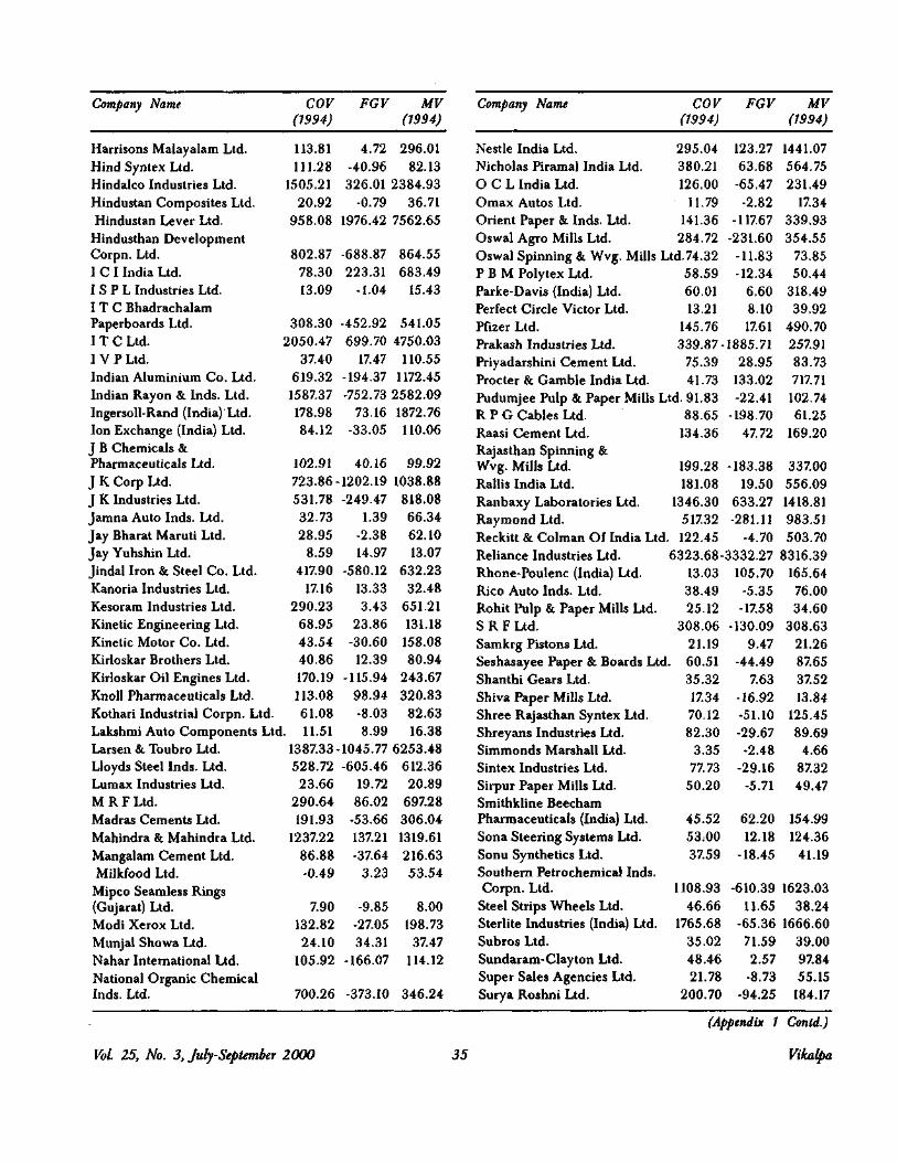
The computed values of independent and dependent variables are given in Appendix 1. Regression results are encouraging. The results of the regression equa-tion are summarized in the Box. The results show that independent variables (COV and FGV) signif-icantly explain the variations in market value

Box: Regression Results of EVA and MVA Relationship

Product-Moment Correlation (Sample Size: 200) 1

Market Value COV FGV (MV) Market Value (MV) 1.000 0.821 -0.279

COV 0.821 1.000 -0.592 FGV -0.279 -0.592 1.000

Regression Results

MV = 63.578 + 2.057 * COV + 0.986 * FGV (1.101) (22.380***) (7.047***)

(R2 = 0.740, Adj.R2 = 0. 279.991*** Durbin-Watson

737, F-statistic Statistic 2.047)

Note: Figures in parenthesis indicate t-statistic. *** indicates significance at 1 per cent level.

Vol. 25, No. 3, July-September 2000 32 Vikalpa

(Adjusted R-squared '= 73.7%). This confirms our hypothesis that market value estimated on the basis of current operational value and future growth value is highly correlated with actual market value. It has already been noted that future growth value depends on expected EVA improvements. In the present study, no projection has been made to estimate future EVAs. The year 1993-94 has been considered as the current year and actual data for next four years (1994-95 to 1997-98) are considered to calculate the future growth value. To calculate EVA for the four-year period (1994-95 to 1997-98), weighted average cost of capital of 1993-94 has been consid-ered. However, the same regression can be carried on the basis of estimated EVAs for future periods. For that purpose, a number of assumptions are to be made to project growth.

A look at the COV and FGV figures would tell us the market implied growth potential of a company. Consider a few examples as listed in Table 4. Table 4: COV, FGV, and Market Value of

Some Companies Rs Crore

COV FGV Market Value

Ashok Leyland 788.27 -598.65 2282.15Hindustan Lever Ltd. (HLL) 958.08 1976.42 7562.65Procter & Gamble India Ltd. (P&G) 41.73 133.02 717.71TISCO 3866.62 -594.24 10296.28Wipro Ltd. 112.22 218.68 82.46

HLL, P&G, and Wipro have future growth potential. FGV is twice that of COV for HLL and Wipro . For P&G, FGV is more than three t imes of COV. The improvement in EVA is greater for P&G. Ashok Leyland and TISCO, on the other hand, have negative FGV figures. In case of Ashok Leyland, the negative FGV is more than 70 per cent of COV figure. It implies that whatever current EVA the company has been able to achieve, it could not generate positive EVAs for future years (1994-95 to 1997-98, in this case). The company does not have encouraging growth prospects. TISCO also shows negative growth prospect. But, its current opera-tional value (for 1993-94, in this case) is quite high. TISCO signifies a typical case of a steel company in India in 90s . Every company in th is indus t ry is passing through a difficult phase — excess capac-ity, inventory pile up, dumping by foreign players, etc. The FGV figure tells that story. Appendix 1, therefore, gives a bet ter picture of a company's

current state of affairs and future growth potential. It sends a clear message — it is important to earn positive EVA but i t is more important to achieve a sustained improvement in EVA. The market value (end of 1993-94) of TISCO is significantly higher than its COV. This does not imply that the share price of TISCO was increasing throughout. In fact, share price of TISCO, which was Rs 193.75 as on March 31, 1994, had fallen to Rs 149.20 as on March 31, 1998. The negative FGV of TISCO captures this fall in share price.

The t-statistics of COV and FGV is significant at one per cent level and the constant is insignificant. This implies that COV and FGV significantly explain the market value of the sample. The Durbin-Watson value also justifies the relationship. An important feature to be noted in this result is that the coefficient of EGV is lower than that of COV. It implies that market value of most of the firms in our sample is a reflection of more of current operational value and less of future growth value. It further implies that the firms in our sample have less market implied growth potential.

Conclusion

However, Appendix 1 also reveals a darker side. There exists a huge gap in many cases between actual market value and the sum total of COV and FGV. For example, in case of HLL, the market value (end of 1993-94) was Rs 7562.65 crore and the FGV was only Rs 1976.42 crore. It implies that FGV has failed in these cases to capture the growth potential factored in the market value of HLL. Another possible explanation for FGVs poor predictive power could be that FGVs are calculated here on the basis of actual operating results of the firms during the period 1994-95 to 1997-98. A longer time horizon and calculation of FGV on the basis of expected future EVAs might produce a better relationship between FGV and market value. The market cap-italization factors in a longer time horizon and capilatizes the growth potential of a firm during the future period. Computing FGV only on the basis of four-year data (1994-95 to 1997-98) might have led to underestimation of future growth potential. We have not attempted here to estimate future EVAs simply because that exercise would involve more assumptions. In the absence of published informa-tion about equity analysts' future projections of firms' performance, it would have been very difficult to estimate economic parameters .of these 200 sample

Vol. 25, No. 3, July-September 2000 33 Vikalpa

firms drawn from diverse industries. Estimating future EVAs for these firms, then, would require some generalization of assumptions. Such an effort

Appendix 1: Computed Values ofIndependent and Dependent Variables

Company Name COV FGV MV (1994) (1994)

Company Name COV FGV MV (1994) (1994)

AFT Industries Ltd. 85.43 Abbott Laboratories (India) Ltd. 22.37 Advani-Oerlikon Ltd. 51.36 Albert David Ltd. 22.16 Alfa Laval (India) Ltd. 126.10 Amtek Auto Ltd. 20.53 Andhra Pradesh Paper Mills Ltd. 65.64 Apollo Tyres Ltd. 233.35 Arvind Mills Ltd. 1262.52 Asea Brown Boveri Ltd. 277.95 Ashok Leyland Ltd. 788.27 Asian Coffee Ltd. 33.81 Asian Paints (India) Ltd. 288.42 Associated Cement Cos. Ltd. 895.76 Astra-Idl Ltd. 24.06 Autolite (India) Ltd. 36.66 Automobile Corpn. Of Goa Ltd. 31.74 BASF India Ltd. 104.77 Bajaj Auto Ltd. 1200.29 Banco Products (India) Ltd. 32.67 Baroda Rayon Corpn. Ltd. 231.68 Bayer (India) Ltd. 203.63 Berger Paints India Ltd. 44.21 Bharat Bijlee Ltd. 26.48 Bharat Forge Ltd. 323.57 Bharat Gears Ltd. 24.06 Bharat Seats Ltd. 14.70 Bimetal Bearings Ltd. 44.88 Birla Corporation Ltd. 284.85 Birla Yamaha Ltd. 24.63 Blow Plast Ltd. 46.63 Blue Star Ltd. 64.10 Bombay Burmah Trdg. Corpn. Ltd. Bombay Dyeing & Mfg. Co. Ltd. 710.94 Britannia Industries Ltd. 102.94 Burroughs Wellcome (India) Ltd. 71.91 Cadbury India Ltd. 42.67 Camlin Ltd. 21.22 Caprihans India Ltd. 76.03 Carrier Aircon Ltd. 33.55 Castrol India Ltd. 325.54

Ceat Ltd. Century Textiles & Inds. Ltd. Cheminor Drugs Ltd. Cimmco Birla Ltd. Cipla Ltd. Clutch Auto Ltd. Colgate-Palmolive (India) Ltd. D C W Ltd. Dalmia Cement (Bharat) Ltd. Deccan Cements Ltd. Denso India Ltd. Dewan Rubber Inds. Ltd. Dr. Reddy'S Laboratories Ltd. Duphar-Interfran Ltd. E I D-Parry (India) Ltd. E Merck (India) Ltd. East Coast Steel Ltd. Elgitread (India) Ltd. Escorts Ltd. Essar Steel Ltd. Eurotex Industries & Exports Ltd. Falcon Tyres Ltd. Finolex Cables Ltd. Forbes Gokak Ltd. Fulford (India) Ltd. G K N Invel Transmissions Ltd. G S L (India) Ltd. Gabriel India Ltd. Gajra Bevel Gears Ltd. German Remedies Ltd. Godfrey Phillips India Ltd. Goetze (India) Ltd. Gontermann-Peipers (India) Ltd. Goodricke Group Ltd. Goodyear India Ltd. Govind Rubber Ltd. Grasim Industries Ltd. Greaves Ltd. Gujarat Ambuja Cements Ltd. Gujarat Lyka Organics Ltd. Hardcastle & Waud Mfg. Co. Ltd.

(Appendix 1 Contd.)

Vol. 25, No. 3, July-September 2000 34 Vikalpa

might have been counter-productive. Therefore, the above results could be considered keeping in mind these limitations.

534.13 1582.42 112.07 174.50 281.45 28.30 409.41 175.33 120.25 29.41 23.29 124.55 330.07 31.11 192.51 385.12 34.67 38.86 267.25 4095.27

54.65•1594.72

-37.38-84.20

545.43-3.45-2.08

-108.60-46.9110.0510.06

-74.4281.64

-14.66-186.60

207.11-24.2218.24

-113.413449.07

-1.30 -5.41 -273.62 -27.77 11.49 -4.21 -63.38 -26.61 -0.61 160.55 116.67 -10.43 -108.27 -17.60 -19.37 -8.41 -838.57 -44.93 -231.79 -96.92

854.131140.23

170.26138.0691.0332.91

6416.90263.03296.33

42.16105.68121.58291.1559.28

370.14297.9532.4436.20

514.154075.24

72.9713.67

254.20427.8735.9897.3589.26

104.1022.49

263.15349.13127.9920.62

438.41107.10111.66

5573.31365.35991.7326.39

75.70 60.18 76.29 38.40

874.97 17.74

102.88637.31

2054.38637.52

2282.1577.05

528.20824.83

33.89 51.12 51.31

284.831660.82

20.64123.13711.2733.5447.13

695.3143.6215.26

137.86919.15 47.24 50.26

27.634.15

22.86-15.94-96.46

9.86-20.51147.39

-847.74-66.08

-598.65-10.02160.10

-645.9030.48

-46.435.27

-28.21617.92

9.33-235.60-45.2820.88-0.28

-148.0829.59-1.33

-14.03-255.33

1.75-33.5315.44

35.62 26.95 269.29 139.64 13.80 34.89 94.06 72.65 11.10 129.11 107.29 87.40 25.75 88.65 77.05 69.30 2398.06 230.28 914.55 79.60

60.09 -43.07 44.46

-490.02 1649.7449.16 511.03 8.98

59.52 16.42

-118.79 66.91

279.35

193.40233.36

29.6188.51

146.74453.63 11.33 -5.41 15.99

Company Name COV FGV MV Company Name COV FGV MV (1994) (1994) (1994) (1994)

T I L Ltd. 54. 94 28 .21 74.14 VST Industries Ltd. 160.72 -88. 65 752.41

T T K Pharma Ltd. 66.67 1 .36 65.06 Vardhman Spinning & TVS Srichakra Ltd. 15. 34 9 .31 17.48 General Mills Ltd. 265 .16 -30. 98 224.47Talbros Automotive Videocon Appliances Ltd. 497.87 -114.68 669.74Components Ltd. 10, ,7 5 .36 12.90 Vikrant Tyres Ltd. 86. ,56 51. 03 160.15Tata Chemicals Ltd. 2204 .1 851 .43 4277.06 Voltas Ltd. 361. 08 -194.52 729.51Tata Engineering & Warren Tea Ltd. 51. 95 28.15 327.02Locomotive Co. Ltd. 1774. 63 -100 .01 5261.92 Tata Infotech Ltd. 80. 55 59 .54 103.26 West Coast Paper Mills Ltd. 46. 29 19. 39 13.11Tata Iron & Steel Co. Ltd. 3866. 62 - .2410296.28 Wimco Ltd. 75. 25 -55. 22 181.29Tata Tea Ltd. 552. 24 14 .58 1777.20 Wipro Ltd. 112. 22 218. 68 82.46Tata-Yodogawa Ltd. 32 .1 -2 .87 62.94 Z F Steering Gear (India) Ltd. 8. 39 -9.37 18.44Ucal Fuel Systems Ltd. 32. ,0 23 .37 50.24 Zuari Industries Ltd. 254. 44 168.14 328.22Uttam Steel Ltd. 194 .1 -161 .11 198.44 Ambalal Sarabhai 103. ,56 - 55 176.72V D O India Ltd. 46. 44 -21.51 33.08 Dee Pharma 41.57 - 52 26.24VIP Industries Ltd. 97.43 9 .76 126.14 Gujarat Themis -6. ,82 3. 34 96.03

References Banerjee, A (1999). "Economic Value Added and Shareholder

Wealth: An Empirical Study of Relationship," Paradigm, Vol 3, No 1, January-June.

Dodd, James L and Chen, Shimin (1996). "EVA: A New Panacea?" Business and Economic Review, Vol 42 , July-September.

Ehrbar, Al (1998). EVA: The Real Key to Creating Wealth, John Wiley & Sons, First Edition.

Grant, J L (1996). "Foundations of EVA for Investment Managers," The Journal of Portfolio Management, Vol 23, Fall Issue.

Hamel, Gary (1997). "Killer Strategies that Make Sharehold-ers Rich," Fortune, June 23.

Kondragunta, Chaith S (2000). "Winning with EVA," Busi-ness Today, February 22.

Lehn, K and Makhija, A K (1996). "EVA and MVA as Per-formance Measures and Signals for Strategic Change," Strategy and Leadership, Vol 24, May-June.

Lev, Baruch (1999). "R&D and Capital Markets," Journal of Applied Corporate Finance, Vol 11, No 4, Winter.

McCormack, John L and Vytheeswaran, Jawanth (1998). "How to Use EVA in the Oil and Gas Industry,"/oama/ of Applied Corporate Finance, Vol 11, No 3, Fall.

Miller, Merton and Modigliani, Franco (1961). "Dividend Policy, Growth and the Valuation of Shares," Journal of Business, Vol 34, No 4, October.

Milunovich, Steven and Tsuei, Albertz (1996). "EVA in the Computer Industry,"Journal of Applied Corporate Finance, Vol 9, No 3, Fall.

O'Byrne, Stephen F (1996). "EVA and Market Value.Vour-nal of Applied Corporate Finance, Vol 9, No 3, Spring.

Rappaport, Alfred (1986). Creating Shareholder Value: The New Standard for Business Performance, Chapter 5, First Edition, New York: The Free Press.

RBI (1996-97). Report on Currency and Finance, Vol II. RBI (1997-98). Report on Currency and Finance, Vol II. Sharpe, W E (1964). "Capital Asset Prices: A Theory of

Market Equilibrium under Conditions of Risk," Journal of Finance, Vol 19.

Sirower, Mark L and O'Byrne, Stephen F (1998). "The Measurement of Post-Acquisition Performance: Toward a Value-based Benchmarking Methodology,"Journal of Applied Corporate Finance, Vol 11, No 2, Summer.

Stewart, Bennett G III (1991). "The Quest for Value," Harper Business, USA.

Tully, Shawn (1993). "The Real Key to Creating Wealth," Fortune, September 20.

Uyemura, Kantor and Petit, Justin (1996). "EVA for Banks: Value Creation, Risk Management, and Profitability Measurement," Journal of Applied Corporate Finance, Vol 9, No 2, Summer.

Wallace James S (1997). Adopting Residual Income Based Com-pensation Plans: Evidence of Effects on Managerial Actions, Working Paper, University of California, USA.

Vol. 25, No. 3, July-September 2000 36 Vikalpa