research article adaptive speed control design for...

Hindawi Publishing CorporationMathematical Problems in EngineeringVolume 2013 Article ID 698050 15 pageshttpdxdoiorg1011552013698050

Research ArticleAdaptive Speed Control Design for Brushed Permanent MagnetDC Motor Based on Worst-Case Analysis Approach

Sheng Zeng

Research and Development Department of Critical Care Engineering CareFusion Yorba Linda CA 92886 USA

Correspondence should be addressed to Sheng Zeng shengzengcarefusioncom

Received 30 April 2012 Revised 23 July 2012 Accepted 23 August 2012

Academic Editor Pedro Ribeiro

Copyright copy 2013 Sheng Zeng This is an open access article distributed under the Creative Commons Attribution License whichpermits unrestricted use distribution and reproduction in any medium provided the original work is properly cited

This paper presents the adaptive controller design for brushed permanent magnet DCmotor used in velocity-tracking applicationsbased on worst-case approach We first formulate the robust adaptive control problem as a nonlinear119867infin-control problem underimperfect state measurement and then solve it using game-theoretic approach The controller guarantees the boundedness ofclosed-loop signals with bounded exogenous disturbances and achieves desired disturbance attenuation level with respect to theunmeasured exogenous disturbance inputs and the measured disturbance inputs The strong robustness properties are illustratedby a simulation example

1 Introduction

Permanentmagnet brushedDC (PMBDC)motors are widelyused in real world applications and particularly in the high-volume commercial products which is due to the PMBDCmotorsrsquo better cost-to-performance ratio than most othermotors However the structure of these permanent mag-netic motors induces several uncertainties such as unmod-elled nonlinear dynamics and undesired commutationdenttorques The magnets losedegrade their magnetic propertiesover time and the motor constant varies with the changesof temperature and operating conditions Moreover the everincreasing control demands for high-efficiency and low-costrequired to run the PMBDC motor at its technical limit Allabove design challenges call for a robust adaptive controllerformotion control applications over awide range of operatingconditions

Adaptive control attracted a lot of research attention incontrol theory since 1970sThe classic adaptive control designbased on the certainty equivalence approach leads to struc-turally simple adaptive controllers [1 2] and its effectivenessfor linear systems with or without stochastic disturbanceinputs has been demonstrated when long-term asymptoticperformance is considered [3] However early designs basedon this approach were not robust to exogenous disturbance

inputs and unmodeled dynamics [4] Then the stability andthe performance of the closed-loop system becomes animportant issue whichmotivated the study of robust adaptivecontrol in the 1980s and 1990s

Robust adaptive control design is one of the most impor-tant research topics in control theory which addresses thedesign of controllers that are robust to model uncertain-ties and insensitive to the exogenous disturbances Variousadaptive controllers were modified to render the closed-loopsystems robust [5ndash10] Despite their successes they howeverfell short of addressing the disturbance attenuation propertyof the closed-loop system Worst-case analysis-based robustadaptive-control design was motivated by the success of thegame-theoretic approach to 119867

infin-optimal control problems[11] in late 1990s which addresses the disturbance attenuationproperty directly In this approach the robust adaptive con-trol problem is formulated as a nonlinear 119867infin-control prob-lem under imperfect state measurements By cost-to-comefunction analysis it is converted into an119867infin-control problemwith full information measurements This full informationmeasurements problem is then solved using nonlinear designtools for a suboptimal solution This design paradigm hasbeen applied to worst-case parameter identification problems[12] which has led to new classes of parametrized identifiersfor linear and nonlinear systems [13ndash16] It has also been

2 Mathematical Problems in Engineering

applied to adaptive control problems [17ndash21] and offered apromising tool to system subjected to uncertainties

In this paper we study the adaptive control design forpermanent magnet DC motor based on worst-case analysisapproach We first model the permanent magnet DC motorservo system which is linear in all of the uncertainties Wethen formulate the robust adaptive control problem as anonlinear 119867infin-control problem under imperfect state mea-surements and apply the cost-to-come function analysis toderive the worst-case identifier and state estimator The con-trol design of the plant subsystem follows [22] and the adap-tive controller can be obtained by the integrator backstep-ping methodology The robust adaptive controller achievesasymptotic tracking if the disturbances are bounded andof finite energy and guarantees the stability of the closed-loop system with respect to the bounded disturbance inputsand the initial conditions Furthermore the close1d-loop sys-tem admits a guaranteed disturbance attenuation level withrespect to the exogenous disturbance inputs and the mea-sured disturbances where ultimate lower bound for theachievable attenuation performance level is only related tothe noise intensity in the measurement channel of the plantsystem

The balance of the paper is organized as follows InSection 2 we present the formulation of the adaptive controlproblem and discuss the general solution methodology thenwe obtain parameter identifier and state estimator usingthe cost-to-come function analysis in Section 3 In Section 4we derive the adaptive control law based on backsteppingmethod and present the main results on the robustness ofthe system in Section 5 The effectiveness of the proposedapproach is illustrated with an example in Section 6 and thepaper ends with some concluding remarks in Section 7

2 Problem Formulation

We consider a velocity-control problem of a brushed perma-nent magnet DC motor which is described by the followingdynamics

=

[[[

[

minus119863

119897

119869

119870119905

119869

minus119870

119890

119871minus119877

119871

]]]

]

119909 + [

0

1

119871

] 119906 + [

[

1

119869

0

]

]

119879+ (1a)

119910 = [1 0] 119909 + (1b)

where isin R2 is the state vector and represents load shaftangular speed and motor current respectively 119906 isin R is thescalar control input 119910 isin R is the load shaft angular speedmeasurement output 119871 isin R is the motor inductor 119877 isin R

is the armature resistance 119870119890is the back-emf constant 119870

119905is

the motor torque constant 119869 is the motor system inertia119863119897isin

R is the motor-system damping factor = [119879119908

120596

119879119891]1015840

is the arbitrary disturbance vector which is composed ofarbitrary disturbance torque 119879

119908isin R arbitrary disturbance

at the output measurement channel 120596

isin R and frictiondisturbance torque 119879

119891isin R 119879

isin R is the measured or

estimated disturbance torque In this paper we assume the

variables 119870119905 119870

119890 119869 119863

119897 119877 and 119871 are completely unknown or

partially unknownIt is easy to check that the true system is observable con-

trollable a minimal phase system and the transfer functionfrom 119906 to 119910 has relative degree 119903 = 2 And then we canfind a state diffeomorphism 119909 = and a disturbance trans-formation 119908 = by following [22] such that system (1a)and (1b) can be transformed into the following form in the 119909coordinates

119909 = 119860119909 + (11991011986021+ 119906119860

22+ 119860

23) 120579 + 119861119906 + 119863119908 + (2a)

119910 = 119862119909 + 119864119908 (2b)

where 119909 isin R2 is the state vector 119909 = [11990911199092]1015840 = 119879

120579 isin R120590 120590 isin N is the 120590-dimensional vector of unknownparameters of the true system the matrices 119860 119860

21 119860

22 119860

23

119863 119862 and 119864 are of appropriate dimensions known andhave the structure as below

119860 = [11988611

1

11988621

11988622

] 11986022

= [01times120590

11986022 0

]

119861 = [0

1198871199010

] 119862 = [1 0]

(3)

where 11986022 0

is a 120590-dimensional row vector and 1198871199010

isin R Thenthe high-frequency gain of (2a) and (2b) is 119887

0= 119887

1199010+ 119860

22 0120579

Since we consider a trajectory tracking control designproblem we make the following assumption about the refe-rence signal 119910

119889

Assumption 1 The reference trajectory 119910119889 is two times con-

tinuously differentiable Define vector119884119889= [119910

(0)

119889119910(1)

119889119910(2)

119889]1015840

and1198841198890

= [119910119889(0) 119910

(1)

119889(0)]

1015840

The signal119884119889is available for con-

trol design

To guarantee the stability of the closed-loop system andthe boundedness of the estimate of 120579 we assume there is an apriori convex compact set where the parameter vector 120579 liesin

Assumption 2 There exists a known smooth nonnegativeradially unbounded strictly convex function 119875 R120590

rarr Rsuch that the true value 120579 isin Θ = 120579 isin R120590

119875(120579) le 1 For all120579 isin Θ 119887

0= 119887

1199010+ 119860

22 0120579 gt 0

The control objective is to design a robust adaptive con-troller for system (1) such that the output 119910(119905) tracks adesired reference signal 119910

119889(119905) while rejecting the uncertain-

ties (119909(0) 120579 [0infin)

[0infin)

1198841198890 119910

(2)

119889) isin W = R2

times Θ times

C times C times R2

times C comprises the initial state the truevalues of unknown parameters unmeasured disturbancesand themeasured disturbances while all signals in the closed-loop system are uniformly bounded We make the controlobjective precise as follows

Mathematical Problems in Engineering 3

Definition 3 A controller 120583 is said to achieve disturbanceattenuation level 120574 if there exist nonnegative functions119897(119905 120579 119909 119910

[0119905] 119879

[0119905]) and 119897

0(

0 120579

0) such that

sup(119909(0)120579119908

120596[0infin)119879119891[0infin)

119879119908[0infin)

119879[0infin)

)

119869119905

le 0 (4)

where

119869119905

= int

119905

0

((119862119909 minus 119910119889)2

+ 119897 minus 12057421003816100381610038161003816119879119908

1003816100381610038161003816

2

minus 120574210038161003816100381610038161003816119879119891

10038161003816100381610038161003816

2

minus12057421003816100381610038161003816119908120596

1003816100381610038161003816

2

minus 1205742 1003816100381610038161003816119879

1003816100381610038161003816

2

) 119889120591

minus 120574210038161003816100381610038161003816120579 minus 120579

0

10038161003816100381610038161003816

2

1198760

minus 12057421003816100381610038161003816119909 (0) minus

0

1003816100381610038161003816

2

Πminus1

0

minus 1198970

(5)

where 1205790isin Θ is the initial guess of the unknown parameter

vector 1198760gt 0 is the quadratic weighting on the error bet-

ween the true value of 120579 and the initial guess 1205790quantifying

the level of confidence in the estimate 1205790

0is the initial guess

of the unknown initial state 119909(0) Πminus1

0gt 0 is the weighting

on the initial state-estimation error quantifying the level ofconfidence in the estimate

0 |119911|

119876denotes 119911

119879

119876119911 for anyvector 119911 and any symmetric matrix 119876

The control law to system (2a) (2b) is generated by thefollowing control law

119906 (119905) = 120583 (119905 119910[0119905]

[0119905]

) (6)

where 120583 [0infin) times L2times L

2rarr R We denote the class of

these admissible controllers byMClearly when the inequality (4) is achieved we have

1003817100381710038171003817119862119909 minus 119910119889

1003817100381710038171003817

2

2(1003817100381710038171003817119879119908

1003817100381710038171003817

2

2+10038171003817100381710038171003817119879119891

10038171003817100381710038171003817

2

2

+1003817100381710038171003817119908120596

1003817100381710038171003817

2

2+1003817100381710038171003817119879

1003817100381710038171003817

2

2

+10038161003816100381610038161003816120579 minus 120579

0

10038161003816100381610038161003816

2

1198760

+1003816100381610038161003816119909 (0) minus

0

1003816100381610038161003816

2

Πminus1

0

+ 1198620)

minus1

le 1205742

(7)

where sdot2denotesL

2norm and119862

0is a constantWhen

2

and 2are finite 119862119909 minus 119910

1198892is also finite which implies

lim119905rarrinfin

|119862119909 minus 119910119889| = 0 under additional assumptions

The following notation will be used throughout thispaper denotes the estimate of the current state of the sys-tem 119909 denotes the state-estimation error 119909minus 120579 denotes theestimate of the parameter vector 120579 120579 denotes the estimationerror 120579 minus 120579 any function symbol with an ldquoover barrdquo willdenote a function defined in the terms of the transformedstate variables such as 119891(119911) being the identical function as119891(119909) for any matrix 119872 the vector 997888rarr119872 is formed by stackingup its column vectors 119890

119895119894denotes a 119895-dimensional column

vector all of its elements are 0 except its 119894th row is 1 such as11989022

= [0 1]1015840

Let 120585 denote the expanded state vector 120585 = [1205791015840

1199091015840

]1015840 we

have the following expanded dynamics for system (2a) (2b)in view of

120579 = 0

120585 = [0 0

11991011986021+ 119906119860

22+ 119860

23 119860

] 120585

+ [0119861] 119906 + [

0119863]119908 + [

0]

= 119860120585 + 119861119906 + 119863119908 +

(8a)

119910 = [0 119862] 120585 + 119864119908 = 119862120585 + 119864119908 (8b)

The worst-case optimization of the cost function (4) canbe carried out in two steps as depicted in the followingequations

sup(119909(0)120579119908

[0infin)[0infin)

)isinW

119869119905

= sup119910[0infin)

[0infin)

sup(119909(0)120579119908

[0infin))|119910[0infin)

[0infin)

119869119905

(9)

The right-hand supremum operator will be carried out firstIt is the identification design step which will be presented inSection 3 Succinctly stated in this step we will calculate themaximum cost that is consistent with the givenmeasurementwaveform

The left-hand supremum operator will be carried outsecond It is the controller design step whichwill be discussedin Section 4 In this step we use a backstepping method todesign the control input 119906 and prove that all state variablesof the closed-loop system are uniformly bounded in time forany uniformly bounded disturbance input waveforms

This completes the formulation of the robust adaptivecontrol problem Next we turn to the identification designstep in the next section

3 Estimation Design

In this section we present the identification design for theadaptive control problem formulated

In this step themeasurement waveform 119910[0infin)

and [0infin)

are assumed to be known Since the control input is a causalfunction of 119910 and then it is known We ignore termsconsidered to be constant in the estimation design step andset 119897 in (5) to be |120585 minus 120585|

2

119876

+ 2(120585 minus 120585)1015840

1198972+ The equivalent cost

function of (5) is then given by

119869120574119905119891 =int

119905119891

0

(10038161003816100381610038161003816120585 minus 120585

10038161003816100381610038161003816

2

119876

+ 2(120585 minus 120585)1015840

1198972+ minus 120574

2

|119908|2

) d120591minus1205742100381610038161003816100381610038161205850

10038161003816100381610038161003816

2

1198760

(10)

where119876 is amatrix-valuedweighting function 120585 is the worst-case estimates for the expanded state 120585 119897

2is a design function

and is considered to be constant in the estimation designstep The cost function is then of a linear quadratic structureand the robust adaptive control problem becomes an 119867

infin-control of affine quadratic problem which admits a finitedimensional solution


We introduce the value function119882 = |120585minus 120585|2

Σminus1 and then

we can obtain the dynamics of state estimator 120585 and worst-case covariance matrix Σ as below

Σ = (119860 minus 1205772

119871119862)Σ + Σ(119860 minus 1205772

119871119862)1015840

+1

1205742119863119863

1015840

minus1

12057421205772

119871 1198711015840

minus Σ (1205742

1205772

1198621015840

119862 minus 1198621015840

119862 minus 119876)Σ

Σ (0) =1

1205742[119876

00

0119899times120590

Πminus1

0

]

minus1

(11a)

120585 = (119860 + Σ (1198621015840

119862 + 119876)) 120585 + 1205772

(1205742

Σ1198621015840

+ 119871) (119910 minus 119862 120585)

+ 119861119906 + minus Σ (1198621015840

119910119889+ 119876120585)

120585 (0) = [1205790

0

]

(11b)

where 120577 = 1(1198641198641015840

)12 and 119871 is defined as 119871 = [0 119871

1015840

]1015840 where

119871 = 1198631198641015840

Then the cost function (5) can be equivalently written as

119869119905

= minus10038161003816100381610038161003816120585 (119905) minus 120585 (119905)

10038161003816100381610038161003816

2

Σminus1(119905)

+ int

119905

0

(10038161003816100381610038161003816119862 120585 minus 119910

119889

10038161003816100381610038161003816

2

+1003816100381610038161003816120585119888

1003816100381610038161003816

2

119876

minus 1205742

120577210038161003816100381610038161003816119910 minus 119862 120585

10038161003816100381610038161003816

2

minus 120574210038161003816100381610038161003816119908 minus 119908

lowast

(119906[0120591]

119910[0120591]

[0120591]

120585[0120591]

120585[0120591]

120585[0120591]

)10038161003816100381610038161003816

2

)119889120591

(12)

where 120585119888= 120585 minus 120585 which will be determined later to improve

the performance of the adaptive system 119908lowast is the worst-casedisturbance given by

119908lowast

(120591 119906[0120591]

119910[0120591]

[0120591]

120585[0120591]

120585[0120591]

120585[0120591]

)

= 1205772

1198641015840

(119910 minus 119862120585) +1

1205742(119868 minus 120577

2

1198641015840

119864)1198631015840

Σminus1

(120585 minus 120585)

(13)

We partition Σ as

Σ = [Σ Σ

12

Σ21

Σ22

] (14)

and introduceΦ = Σ21Σ

minus1 and Π = 1205742

(Σ22minus Σ

21Σ

minus1

Σ12)

For the boundedness ofΣ wemake the following assump-tion on the weighting matrix 119876

Assumption 4 The weighting matrix 119876 of function 119897 in (5) isgiven by

119876 = Σminus1

[0 00 Δ

]Σminus1

+ [120598Φ

1015840

1198621015840

(1205742

1205772

minus 1)119862Φ 00 0] (15)

where Δ is 2 times 2 positive-definite matrix and 120598 is a scalarfunction defined by

120598 (120591) =

Tr (Σminus1

(120591))

119870119888

119870119888ge 120574

2 Tr (1198760) 120591 ge 0 (16)

Then we have the following differential equation of ΣΦand Π

Σ = minus (1 minus 120598) ΣΦ1015840

1198621015840

(1205742

1205772

minus 1)119862ΦΣ

Σ (0) =1

1205742119876

minus1

0

(17a)

Φ = (119860 minus 1205772

119871119862 minus1

1205742Π119862

1015840

(1205742

1205772

minus 1)119862)Φ

+ 11991011986021+ 119906119860

22+ 119860

23 Φ (0) = 0

(17b)

Π = (119860 minus 1205772

119871119862)Π+Π(119860 minus 1205772

119871119862)1015840

minusΠ1198621015840

(1205772

minus1

1205742)119862Π

+ 1198631198631015840

minus 1205772

1198711198711015840

+ 1205742

Δ Π (0) = Π0

(17c)

The matrix Σ will play the role of worst-case covariancematrix of the parameter estimation error Assumption 4 guar-antees thatΣ is uniformly bounded fromabove anduniformlybounded frombelow away from 0 as depicted in the followinglemma and its proof is given in [14]

Lemma 5 Consider the dynamic equation (17a) for thecovariance mat-rix Σ Let Assumption 4 hold and 120574 ge 120577

minus1Then Σ is uniformly upper and lower bounded as follows

1

119870119888

le Σ (120591) le Σ (0) =1

1205742119876

minus1

0

1205742 Tr (119876

0) le Tr (Σminus1

(120591)) le 119870119888 forall120591 isin [0 119905]

(18)

We define 119904Σ(119905) = Tr((Σ(119905))minus1) and its dynamic is given

by

119904Σ= 120574

2

1205772

(1 minus 120598) 119862ΦΦ1015840

1198621015840

119904Σ(0) = 120574

2 Tr (1198760) (19)

Then 120598(120591) = 119870minus1

119888119904minus1

Σ(120591) which does not require the inversion

of ΣFrom Assumption 4 and (17a) we note that 120574 ge 120577

minus1 Thismeans the quantity 120577

minus1 is the ultimate lower bound on theachievable performance level for the adaptive system usingthe design method proposed in this paper

Assumption 6 If the matrix 119860 minus 1205772

119871119862 is Hurwitz thenthe desired disturbance attenuation level 120574 ge 120577

minus1 If thematrix119860minus120577

2

119871119862 is not Hurwitz then the desired disturbanceattenuation level 120574 gt 120577

minus1


Assumption 7 The initial weightingmatrixΠ0in (17c) is cho-

sen as the unique positive definite solution to the followingalgebraic Riccati equation

(119860 minus 1205772

119871119862)Π + Π(119860 minus 1205772

119871119862)1015840

minus Π1198621015840

(1205772

minus1

1205742)119862Π

+ 1198631198631015840

minus 1205772

1198711198711015840

+ 1205742

Δ = 0

(20)

Then we note that the unique positive-definite solutionof (17c) is time-invariant and equal to the initial value Π

0

Remark 8 To simplify the estimator structure we can choose120598 = 1 so that Σ will be a constant positive-definite matrixand 119904

Σwill be a finite positive constant To further simplify

the identifier the initial weighting matrix Π0is chosen as

the unique positive-definite solutions to its algebraic Riccatiequation (17c) which also implies Σ gt 0 in view of Σ gt 0

To guarantee the boundedness of estimated parameterswithout persistently exciting signals we introduce soft pro-jection design on the parameter estimate We define

120588 = inf 119875 (120579) | 120579 isin R120590

1198871199010

+ 11986022 0

120579 = 0 (21)

By Assumption 2 and Lemma 2 in [23] we have 1 lt 120588 le infinFor any fixed 120588

119900isin (1 120588) we define the open set

Θ119900= 120579 isin R

120590

| 119875 (120579) lt 120588119900 (22)

Our control design will guarantee that the estimate 120579 lies inΘ

119900 which immediately implies |119887

1199010+ 119860

22 0

120579| gt 1198880

gt 0for some 119888

0gt 0 Moreover the convexity of 119875 implies the

following inequality

120597119875

120597120579( 120579) (120579 minus 120579) lt 0 forall 120579 isin R

120590

Θ (23)

We set 1198972= [minus(119875

119903( 120579))

1015840

0]1015840

where

119875119903( 120579) =

1198901(1minus119875(

120579))

((120597119875120597120579) ( 120579))1015840

(120588119900minus 119875 ( 120579))

3forall120579 isin Θ

119900 Θ

0 forall120579 isin Θ

(24)

Then we obtain

120585 = minus Σ[(119875119903( 120579))

1015840

0]1015840

+ 119860 120585 + 119861119906 minus Σ119876120585119888

+ 1205772

(1205742

Σ1198621015840

+ 119871) (119910 minus 119862 120585) +

120585 (0) = [ 1205791015840

01015840

0]1015840

(25)

where 120585119888= 120585 minus 120585

We summarize the estimation dynamics equations below

(119860 minus 1205772

119871119862)Π + Π(119860 minus 1205772

119871119862)

minus Π1198621015840

(1205772

minus1

1205742)119862Π + 119863119863

1015840

minus 1205772

1198711198711015840

+ 1205742

Δ = 0

(26a)

Σ = minus (1 minus 120598) ΣΦ1015840

1198621015840

(1205742

1205772

minus 1)119862ΦΣ Σ (0) =1

1205742119876

minus1

0

(26b)

119904Σ= (120574

2

1205772

minus 1) (1 minus 120598) 119862ΦΦ1015840

1198621015840

119904120590(0) = 120574

2 Tr (1198760)

(26c)

120598 =1

119870119888119904Σ

(26d)

119860119891= 119860 minus 120577

2

119871119862 minus Π1198621015840

119862(1205772

minus1

1205742) (26e)

Φ = 119860119891Φ + 119910119860

21+ 119906119860

22+ 119860

23 Φ (0) = 0 (26f)

120579 = minus Σ119875119903( 120579) minus ΣΦ

1015840

1198621015840

(119910119889minus 119862)

minus[Σ ΣΦ1015840

] 119876120585119888+120574

2

1205772

ΣΦ1015840

1198621015840

(119910 minus 119862) 120579 (0)= 1205790

(26g)

= minus ΦΣ119875119903( 120579) + 119860 minus (

1

1205742Π + ΦΣΦ

1015840

)1198621015840

(119910119889minus 119862)

minus [ΦΣ1

1205742Π + ΦΣΦ

1015840

]119876120585119888

+ (11991011986021+ 119906119860

22+ 119860

23) 120579

+ 1205772

(Π1198621015840

+ 1205742

ΦΣΦ1015840

1198621015840

+ 119871)

times (119910 minus 119862) + + 119861119906 (0) = 0

(26h)For the controller structure simplification the dynamics

for Φ can be implemented as below First we observe thematrix 119860

119891has the same structure as the matrix 119860 Then we

introduce the matrix119872

119891= [119860

11989111990121199012] (27)

where1199012is a 2-dimensional vector such that the pair (119860

119891 119901

2)

is controllable which implies that119872119891is invertible Then the

following prefiltering system for 119910 119906 and generates the Φonline

120578 = 119860119891120578 + 119901

2119910 120578 (0) = 0 (28a)

120582 = 119860119891120582 + 119901

2119906 120582 (0) = 0 (28b)

120578

= 119860119891120578

+ 1199012 120578

(0) = 0 (28c)

Φ = [119860119891120578 120578]119872

minus1

119891119860

21+ [119860

119891120582 120582]119872

minus1

119891119860

22

+ [119860119891120578

120578

]119872minus1

119891119860

23

(28d)


Associated with the above identifier introduce the valuefunction

119882(119905 120585 (119905) 120585 (119905) Σ (119905))

=10038161003816100381610038161003816120585 (119905) minus 120585 (119905)

10038161003816100381610038161003816

2

Σ

minus1

(119905)

=10038161003816100381610038161003816120579 minus 120579 (119905)

10038161003816100381610038161003816

2

Σminus1

(119905)

+ 120574210038161003816100381610038161003816119909 (119905) minus (119905) minus Φ (119905) (120579 minus 120579 (119905))

10038161003816100381610038161003816

2

Πminus1

(29)

whose time derivative is given by

119882 = minus1003816100381610038161003816119862119909 minus 119910

119889

1003816100381610038161003816

2

minus 120574410038161003816100381610038161003816119909 minus 119909 minus Φ (120579 minus 120579)

10038161003816100381610038161003816

2

Πminus1

ΔΠminus1

minus 120598 (1205742

1205772

minus 1)10038161003816100381610038161003816120579 minus 120579

10038161003816100381610038161003816

2

Φ10158401198621015840119862Φ

+ 1205742

|119908|2

+1003816100381610038161003816119862 minus 119910

119889

1003816100381610038161003816

2

+1003816100381610038161003816120585119888

1003816100381610038161003816

2

119876

minus 1205742

12057721003816100381610038161003816119910 minus 119862

1003816100381610038161003816

2

minus 120574210038161003816100381610038161003816119908 minus 119908

lowast

(119905 119906[0119905]

119910[0119905]

[0119905]

120585[0119905]

120585[0119905]

120585[0119905]

)10038161003816100381610038161003816

2

+ 2(120579 minus 120579)1015840

119875119903( 120579)

(30)

We note that the last term in

119882 is nonpositive zero on the setΘ and approaches minusinfin as 120579 approaches the boundary of theset Θ which guarantees the boundness of 120579

Then the cost function can be equivalently written as

119869119905

= 119869119905

+119882(0) minus119882 (119905) + int

119905

0

119882119889120591

= minus10038161003816100381610038161003816120579 minus 120579 (119905)

10038161003816100381610038161003816

2

Σminus1

(119905)

minus 120574210038161003816100381610038161003816119909 (119905) minus (119905) minus Φ (119905) (120579 minus 120579 (119905))

10038161003816100381610038161003816

2

Πminus1

+ int

119905

0

(1003816100381610038161003816119862 minus 119910

119889

1003816100381610038161003816

2

+1003816100381610038161003816120585119888

1003816100381610038161003816

2

119876

minus 1205742

12057721003816100381610038161003816119910 minus 119862

1003816100381610038161003816

2

minus 120574210038161003816100381610038161003816119908 minus 119908

lowast

times (120591 119906[0120591]

119910[0120591]

[0120591]

120585[0120591]

120585[0120591]

120585[0120591]

)10038161003816100381610038161003816

2

+ minus 1205742

||2

) 119889120591

(31)

This completes the identification design step

4 Control Design

In this section we describe the controller design for theuncertain system under consideration Note that we ignoredsome terms in the cost function (5) in the identification stepsince they are constant when 119910 and are given In the controldesign step we will include such terms Then based on thecost function (5) in the Section 2 the controller design is to

guarantee that the following supremum is less than or equalto zero for all measurement waveforms

sup(119909(0)120579119908[0infin)[0infin))isinW

119869119905

le sup119910[0infin)

[0infin)

int

119905

0

(1003816100381610038161003816119862 minus 119910

119889

1003816100381610038161003816

2

+1003816100381610038161003816120585119888

1003816100381610038161003816

2

119876

minus 1205742

12057721003816100381610038161003816119910 minus 119862

1003816100381610038161003816

2

+ minus 1205742

||2

) 119889120591 minus 1198970

(32)

where function (120591 119910[0120591]

[0120591]

) is part of the weighting func-tion 119897(120591 120579 119909 119910

[0120591]

[0120591]) to be designed which is a constant

in the identifier design step and is therefore neglectedBy (32) we observe that the cost function is expressed

in term of the states of the estimator we derived whosedynamics are driven by the measurement 119910 input 119906 mea-sured disturbance and the worst-case estimate for theexpanded state vector 120585 which are signals we either measureor can constructThis is then a nonlinear119867infin-optimal controlproblem under full information measurements Instead ofconsidering 119910 and as the maximizing variable we canequivalently deal with the transformed variable

119907 = [120577 (119910 minus 119862)

] (33)

Then we have

120578 = 119860119891120578 + 119901

2119862 + 119901

2(1198901015840

21119907

120577) (34)

120579 = minus Σ119875119903( 120579) minus ΣΦ

1015840

1198621015840

(119910119889minus 119862)

minus [Σ ΣΦ1015840

] 119876120585119888+ 120574

2

ΣΦ1015840

1198621015840

1205771198901015840

21119907

(35)

= 119860 minus (1

1205742Π + ΦΣΦ

1015840

)1198621015840

(119910119889minus 119862) + 119860

21

120579119862

minus ΦΣ119875119903( 120579) minus [ΦΣ

1

1205742Π + ΦΣΦ

1015840

]119876120585119888+ 119861119906

+ 11986022

120579119906 + ((120577minus2

11986021

120579 + Π1198621015840

+ 1205742

ΦΣΦ1015840

1198621015840

+ 119871) 1205771198901015840

21

+11986023

1205791198901015840

22+ [0

119899times1] ) 119907

(36)

119882 = minus1003816100381610038161003816119862119909 minus 119910

119889

1003816100381610038161003816

2


10038161003816100381610038161003816

2

Πminus1

ΔΠminus1

minus 120598 (1205742

1205772

minus 1)10038161003816100381610038161003816120579 minus 120579

10038161003816100381610038161003816

2

Φ10158401198621015840119862Φ

+1003816100381610038161003816119862 minus 119910

119889

1003816100381610038161003816

2

+1003816100381610038161003816120585119888

1003816100381610038161003816

2

119876

+ 2(120579 minus 120579)1015840

119875119903( 120579)

+ 1205742

||2

+ 1205742

|119908|2

minus 1205742

|119907|2

minus 120574210038161003816100381610038161003816119908 minus 119908

lowast

(119905 119906[0119905]

119910[0119905]

[0119905]

120585[0119905]

120585[0119905]

120585[0119905]

)10038161003816100381610038161003816

2

(37)


The variables to be designed at this stage include 119906 and120585119888 The design for 120585

119888will be carried out last Note that the

structure of 119860 in the dynamics is in strict-feedback formwe will use the backstepping methodology [24] to designthe control input 119906 which will guarantee the global uniformboundedness of the closed-loop system states and the asymp-totic convergence of tracking error

Consider the dynamics of Φ

Φ = 119860119891Φ + 119910119860

21+ 119906119860

22+ 119860

23 Φ (0) = 0 (38)

For ease of the ensuing study we will separate Φ as the sumof several matrices as follows

Φ = Φ119906

+ Φ119910

+ Φ

(39a)

Φ119910

= [119860119891120578 120578]119872

minus1

119891119860

21= [

1205781015840

1198791

1205781015840

1198792

] (39b)

Φ119906

= 119860119891Φ

119906

+ 11990611986022 Φ

119906

(0) = 0 (39c)

Φ

= 119860119891Φ

+ 11986023 Φ

(0) = 0 (39d)

where 119879119894 119894 = 1 2 are 2 times 1-dimensional constant matrices

depending on119860119891119872

119891 and119860

21 ExpressΦ119906 andΦ in terms

of their row vectorsΦ119906

= [Φ1199061015840

1Φ

1199061015840

2]

1015840

andΦ

= [Φ1015840

1Φ

1015840

2]1015840

Then 119862Φ119910

= 1205781015840

1198791 119862Φ119906

= Φ119906

1 and 119862Φ

= Φ

1

We summarized the dynamics for backstepping design inthe following where we have emphasized the dependence ofvarious functions on the independent variables

119904Σ= (120574

2

1205772

minus 1) (1 minus 120598) (1205781015840

1198791+ Φ

119906

1+ Φ

1)

times (1205781015840

1198791+ Φ

119906

1+ Φ

1)1015840

(40a)

120598 =1

119870119888119904Σ

(40b)

Σ = minus (1 minus 120598) Σ(1205781015840

1198791+ Φ

119906

1+ Φ

1)1015840

times (1205742

1205772

minus 1) (1205781015840

1198791+ Φ

119906

1+ Φ

1) Σ

(40c)

120579 = 120575 (119910119889minus

1 120578 Φ

1 Φ

119906

1 120579

997888rarrΣ)

+ 120593(120578997888rarrΦ

997888rarrΦ

119906

997888rarrΣ)119876120585

119888+ 120581 (120578Φ

1 Φ

119906

1997888rarrΣ) 119907

(40d)

120578 = 119860119891120578 + 119901

21+ 119901

2(1198901015840

21119907

120577) (40e)

1=

2+ 119891

1(119910

119889minus

1

1 120579 120578 Φ

1 Φ

119906

1997888rarrΣ)

+ 9848581(120578

997888rarrΦ

997888rarrΦ

119906

997888rarrΣ)119876120585

119888

+ ℎ1( 120579 120578 Φ

1 Φ

119906

1997888rarrΣ) 119907

(40f)

2= 119886

222+ (119887

1199010+ 119860

220

120579) 119906

+ 1198912(119910

119889minus

1

1

2 120579 120578 Φ

1 Φ

2 Φ

119906

1 Φ

119906

2997888rarrΣ)

+ 9848582(120578

997888rarrΦ

997888rarrΦ

119906

997888rarrΣ)119876120585

119888

+ ℎ2( 120579 120578 Φ

1 Φ

2 Φ

119906

1 Φ

119906

2997888rarrΣ) 119907

(40g)

Φ119906

1= 120595

1(Φ

119906

1) + Φ

119906

2 (40h)

Φ

1= 120603

1(Φ

1) + Φ

2+ 119890

1015840

21119860

231198901015840

22119907 (40i)

where the nonlinear functions 120575 1198911 and 119891

2are smooth as

long as 120579 isin Θ119900 the nonlinear functions 120593 120581 984858

1 984858

2 ℎ

1 ℎ

2

1205951 and 120603

1are smooth Here we use Φ

119906

1 Φ119906

2 Φ

1 and Φ

2

as independent variables instead of 120582 1205781 for the clarity of

ensuing analysisWe observe that the above dynamics is linear in 120585

119888 which

will be optimatized after backstepping design Σ 119904Σ Φ and

120579 will always be bounded by the design in Section 3 thenthey will not be stabilized in the control design Φ119906 is notnecessary bounded since the control input 119906 appeared intheir dynamics it can not stabilzed in conjunction with

using backstepping Hence we assume it is bounded andprove later that it is indeed so under the derived control law

The following backstepping design will achieve the 120574 levelof disturbance attenuation with respect to the disturbance 119907

Step 1 In this step we try to stabilize 120578 by virtual control law1= 119910

119889 Introduce variable 120578

119889 as the desired trajectory of 120578

which satisfies the dynamics

120578119889= 119860

119891120578119889+ 119901

2119910119889 120578

119889(0) = 0

2 times 1 (41)

Define the error variable 120578 = 120578 minus 120578119889 Then 120578 satisfies the

dynamics

120578 = 119860119891120578 + 119901

2(1198901015840

21119907

120577) + 119901

2(

1minus 119910

119889) (42)

By [14] the following holds

Lemma 9 Given any Hurwitz matrix 119860119891 there exists a

positive-definite matrix 119884 such that the following generalizedalgebraic Riccati equation admits a positive-definite solution119885

1198601015840

119891119885 + 119885119860

119891+

1

12057421205772119885119901

21199011015840

2119885 + 119884 = 0 (43)

Note that 119860119891in (42) is a Hurwitz matrix then we define

the following value function in terms of the positive-definitematrix 119885

1198810(120578) =

10038161003816100381610038161205781003816100381610038161003816

2

119885 (44)

Then its time derivative is given by

1198810= minus

10038161003816100381610038161205781003816100381610038161003816

2

119884+ 120574

2

|119907|2

minus 12057421003816100381610038161003816119907 minus 120584

0

1003816100381610038161003816

2

+ 21205781015840

119885119901119899(

1minus 119910

119889) (45)


where

1205840(120578) =

1

1205742120577119890211199011015840

2119885120578 (46)

If 1is control input then we may choose the control law

1= 119910

119889 (47)

and the design achieves attenuation level 120574 from the distur-bance 119907 to the output 11988412

(120578 minus 120578119889) This completes the virtual

control design for the 120578 dynamics

Step 2 Define the transformed variable

1199111=

1minus 119910

119889 (48)

which is the deviation of 1from its desired trajectory 119910

119889

Then the time derivative of 1199111is given by

1199111= 119891

1(119911

1 119910

119889 120579 120578 Φ

1 Φ

119906

1997888rarrΣ) +

2minus 119910

(1)

119889

+ 9848581(120578

997888rarrΦ

997888rarrΦ

119906

997888rarrΣ)119876120585

119888+ ℎ

1( 120579 120578 Φ

1 Φ

119906

1997888rarrΣ) 119907

(49)

where the function 1198911is defined as

1198911(119911

1 119910

119889 120579 120578 Φ

1 Φ

119906

1997888rarrΣ)

= 1198911(119910

119889minus

1

1 120579 120578 Φ

1 Φ

119906

1997888rarrΣ)

(50)

Introduce the value function for this step

1198811= 119881

0+1

21199112

1(51)

whose derivative is given by

1198811= minus

10038161003816100381610038161205781003816100381610038161003816

2

119884+ 120574

2

|119907|2

minus 12057421003816100381610038161003816119907 minus 120584

0

1003816100381610038161003816

2

+ 21205781198851199011198991199111

+ 1199111(

2minus 119910

(1)

119889+ 119891

1+ 984858

1119876120585

119888+ ℎ

1119907)

= minus1199112

1minus10038161003816100381610038161205781003816100381610038161003816

2

119884minus 120573

11199112

1+ 119911

11199112+ 120589

1015840

1119876120585

119888

+ 1205742

|119907|2

minus 12057421003816100381610038161003816119907 minus 120584

1

1003816100381610038161003816

2

(52)

where

1199112=

2minus 119910

(1)

119889minus 120572

1 (53a)

1205841(119911

1 120579 120578 120578 Φ

1 Φ

119906

1997888rarrΣ) = 120584

0+

1

21205742ℎ1015840

11199111 (53b)

1205721(119911

1 119910

119889 120579 120578 120578 Φ

1 Φ

119906

1997888rarrΣ 119904) = minus 119911

1minus 120573

11199111minus 2119901

1015840

119899119885120578

minus 1198911minusℎ

11205840minus

1

41205742ℎ1ℎ1015840

11199111

(53c)

1205731(119911

1 119910

119889 120579 120578 120578 Φ

1 Φ

119906

1997888rarrΣ 119904) ge 119888

1205731

gt 0 (53d)

1205891(119911

1 119910

119889 120578 120578 Φ

1 Φ

119906

997888rarrΣ) = 984858

1015840

11199111 (53e)

where 1198881205731

is any positive constant and the nonlinear function1205731is to be chosen by the designer Note that the function 120572

1is

smooth as long as 120579 isin Θ119900 If

2were the actual controls then

we would choose the following control law

2= 119910

(1)

119889+ 120572

1 (54)

and set 120585119888= 0 to guarantee the dissipation inequality with

supply rate

minus10038161003816100381610038161

minus 119910119889

1003816100381610038161003816

2

minus10038161003816100381610038161205781003816100381610038161003816

2

119884minus 120573

11199112

1+ 120574

2

1199072

(55)

This completes the second step of backstepping design

Step 3 At this step the actual control appears in the derivativeof 119911

2 which is given by

1199112= 119886

222+ (119887

1199010+ 119860

220

120579) 119906

minus 119910(2)

119889+ 120594

21+ 2120574

2

12059422119907 + 120594

23119876120585

119888

(56)

where 12059421 120594

22 and 120594

23are given as follows

12059421

= 1198912minus120597120572

1

1205971

(1198911+

2) minus

1205971205721

120597119910119889

119910(1)

119889

minus120597120572

1

120597 120579

120575 minus120597120572

1

120597120578(119860

119891120578 + 119901

21199111)

minus120597120572

1

120597120578(119860

119891120578 + 119901

21) minus

1205971205721

120597Φ

1

(Φ

2+ 120603

1)1015840

minus120597120572

1

120597Φ119906

1

(Φ119906

2+ 120595

1)1015840

minus120597120572

1

120597997888rarrΣ

(120598 minus 1)

times

997888997888997888997888997888997888997888997888997888997888997888997888997888997888997888997888997888997888997888997888997888997888997888997888997888997888997888997888997888997888997888997888997888997888997888997888997888997888997888997888997888997888997888997888997888997888997888rarr

(Σ(1205781015840

1198791+Φ

1+ Φ

119906

1)1015840

(1205742

1205772

minus1) (1205781015840

1198791+Φ

1+Φ

119906

1) Σ)

minus120597120572

1

120597119904Σ

(1205742

1205772

minus 1) (1 minus 120598) (1205781015840

1198791+ Φ

1+ Φ

119906

1)

times (1205781015840

1198791+ Φ

1+ Φ

119906

1)1015840

12059422

=1

21205742(ℎ

2minus120597120572

1

1205971

ℎ1minus120597120572

1

120597 120579

120581 minus120597120572

1

120597120578

11990121198901015840

21

120577

minus120597120572

1

120597120578

11990121198901015840

21

120577minus

1205971205721

120597Φ

1

1198601015840

23119890221198901015840

22)

12059423

= 9848582minus120597120572

1

1205971

9848581minus120597120572

1

120597 120579

120593

(57)

Introduce the following value function for this step

1198812= 119881

1+1

21199112

2 (58)

Its derivative can be written as

1198812= minus119911

2

1minus10038161003816100381610038161205781003816100381610038161003816

2

119884minus

2

sum

119895=1

1205731198951199112

119895+ 120574

2

|119907|2

minus 12057421003816100381610038161003816119907 minus 120584

2

1003816100381610038161003816

2

+ 1205891015840

2119876120585

119888

(59)


with the control law defined by

119906 = 120583 (1199111 119911

2

1

2 119910

119889 119910

(1)

119889

120579 120578 120578 Φ

1 Φ

2 Φ

119906

1 Φ

119906

119903

997888rarrΣ 119904

Σ)

= minus1

1198871199010

+ 119860220

120579

(119886222minus 119910

(2)

119889minus 120572

2)

(60)

where

1205722= minus 120594

21minus 2120574

2

120594222

minus 21205742

120594221

1198901015840

211205841

minus 1205742

1205942

2211199112minus 120573

21199112minus 119911

1

(61)

1205842= 120584

1+ 119890

21120594221

1199112 (62)

where 12059422

= [120594221

120594222

] Clearly the functions 120583 12059421 120594

22

12059423 120584

2 and 120589

2are smooth as long as 120579 isin Θ

119900

This completes the backstepping design procedure

For the closed-loop adaptive nonlinear system we havethe following value function

119880 = 1198812+119882 =

10038161003816100381610038161003816120579 minus 120579

10038161003816100381610038161003816

2

Σminus1+ 120574

210038161003816100381610038161003816119909 minus minus Φ (120579 minus 120579)

10038161003816100381610038161003816

2

Πminus1

+10038161003816100381610038161205781003816100381610038161003816

2

119885+1

2

2

sum

119895=1

(119895minus 119910

(119895minus1)

119889minus 120572

119895minus1)2

(63)

where we have introduced 1205720= 0 for notational consistency

The time derivative of this function is given by

119880 = minus1003816100381610038161003816119862119909 minus 119910

119889

1003816100381610038161003816

2


10038161003816100381610038161003816

2

Πminus1

ΔΠminus1

minus 120598 (1205742

1205772

minus 1)10038161003816100381610038161003816120579 minus 120579

10038161003816100381610038161003816

2

Φ10158401198621015840119862Φ

+ 2(120579 minus 120579)1015840

119875119903( 120579) +

10038161003816100381610038161205851198881003816100381610038161003816

2

119876

+ 1205891015840

119903119876120585

119888minus10038161003816100381610038161205781003816100381610038161003816

2

119884

minus

2

sum

119895=1

1205731198951199112

119895+ 120574

2

|119908|2

+ 1205742

||2

minus 120574210038161003816100381610038161003816119908 minus 119908

lowast

(119905 119906[0119905]

119910[0119905]

[0119905]

120585[0119905]

120585[0119905]

120585[0119905]

)10038161003816100381610038161003816

2

minus 12057421003816100381610038161003816119907 minus 120584

2

1003816100381610038161003816

2

= minus1003816100381610038161003816119862119909 minus 119910

119889

1003816100381610038161003816

2


10038161003816100381610038161003816

2

Πminus1

ΔΠminus1

minus 120598 (1205742

1205772

minus 1)10038161003816100381610038161003816120579 minus 120579

10038161003816100381610038161003816

2

Φ10158401198621015840119862Φ

+ 2(120579 minus 120579)1015840

119875119903( 120579) +

1003816100381610038161003816100381610038161003816120585119888+1

21205892

1003816100381610038161003816100381610038161003816

2

119876

minus1

4

100381610038161003816100381612058921003816100381610038161003816

2

119876

minus10038161003816100381610038161205781003816100381610038161003816

2

119884minus

2

sum

119895=1

1205731198951199112

119895+ 120574

2

|119908|2

+ 1205742

||2

minus 120574210038161003816100381610038161003816119908 minus 119908

lowast

(119905 119906[0119905]

119910[0119905]

[0119905]

120585[0119905]

120585[0119905]

120585[0119905]

)10038161003816100381610038161003816

2

minus 12057421003816100381610038161003816119907 minus 120584

2

1003816100381610038161003816

2

(64)

Then the optimal choice for the variables 120585119888and 120585 are

120585lowast

119888= minus

1

21205892lArrrArr 120585

lowast

= 120585 minus1

21205892 (65)

which yields that the closed-loop system is dissipative withstorage function 119880 and supply rate

minus10038161003816100381610038161199091

minus 119910119889

1003816100381610038161003816

2

+ 1205742

|119908|2

+ 1205742

||2

(66)

Furthermore the worst case disturbance with respect to thevalue function 119880 is given by

119908opt = 1205771198641015840

1198901015840

211205842+

1

1205742(119868 minus 120577

2

1198641015840

119864)1198631015840

Σminus1

(120585 minus 120585)

+ 1205772

1198641015840

119862 ( minus 119909)

(67)

opt = 119890221205842 (68)

5 Main Result

For the adaptive control law with 120585119888chosen according to (65)

the closed-loop system dynamics are

119883 = 119865 (119883 119910(2)

119889) + 119866 (119883)119908 + 119866

(119883) (69)

119883 is the state vector of the close-loop system and given by

119883 = [1205791015840

1199091015840

119904Σ

1205791015840

1015840

1205781015840

1205781015840

1198891205781015840

997888rarrΦ

119906

1015840 larr997888Σ

1015840

119910119889

119910(1)

119889

]

1015840

(70)

which belongs to the setD = 119883 | Σ gt 0 119904Σgt 0 120579 isin Θ

119900119865

and119866 are smoothmapping ofDtimesR andD respectively andwith the initial condition 119883(0) = 119883

0isin D

0= 119883

0isin D | 120579 isin

Θ 1205790isin Θ Σ(0) = 120574

minus2

119876minus1

0gt 0Tr((Σ(0))minus1) le 119870

119888 119904

Σ(0) =

1205742 Tr(119876

0)

Since (64) holds the value function119880 satisfies Hamilton-Jacobi-Isaacs equation for all119883 isin D for all 119910(2)

119889isin R

120597119880

120597119883(119883) 119865 (119883 119910

(2)

119889) +

1

41205742

120597119880

120597119883(119883) [119866 (119883) 119866

119908(119883)]

sdot [119866 (119883) 119866119908(119883)]

1015840

(120597119880

120597119883(119883))

1015840

+ 119876 (119883 119910(2)

119889) = 0

(71)


where 119876 D timesR rarr R is smooth and given by

119876(119883 119910(2)

119889) =

100381610038161003816100381611990911minus 119910

119889

1003816100381610038161003816

2

+(10038161003816100381610038161003816120585 minus 120585

10038161003816100381610038161003816

2

119876

+119875119903( 120579)

10038161003816100381610038161205781003816100381610038161003816

2

119884minus2(120579 minus 120579)

1015840

times119875119903( 120579)+

2

sum

119895=1

1205731198951199112

119895+1

4

100381610038161003816100381612058921003816100381610038161003816

2

119876)

(72)

Although the value function 119880 satisfies an Hamilton-Jacobi-Isaacs equation we cannot deduce the stability androbustness properties of the closed-loop system directly from(64) since119880 is not a positive-definite function of the closed-loop state vector 119883 We will use the following theorem toprecisely state the strong stability properties of the closed-loop adaptive system

Theorem 10 Consider the robust adaptive control problemformulated in Section 2 with Assumptions 1ndash7 holding Therobust adaptive controller 120583 defined by (60) with the optimalchoice for the worst-case estimate 120585 defined by (65) achievesthe following strong robustness properties for the closed-loopsystem

(1) The controller 120583 achieves disturbance attenuationlevel 120574 for any uncertainty quadruple (119909(0) 120579 119908

[0infin)

[0infin)

1198841198890 119910

(2)

119889) isin W

(2) Given a 119888119908

gt 0 there exists a constant 119888119888gt 0 and a

compact set Θ119888sub Θ

119900 such that for any uncertainty

(119909(0) 120579 [0infin)

[0infin)

119884119889) with

|119909 (0)| le 119888119908 | (119905)| le 119888

119908 | (119905)| le 119888

119908

1003816100381610038161003816119884119889(119905)

1003816100381610038161003816 le 119888119908 forall119905 isin [0infin)

(73)

all closed-loop state variables 119909 120579 Σ 119904Σ 120578 120578 120578

119889

and 120582 are bounded as follows for all 119905 isin [0infin)

|119909 (119905)| le 119888119888 | (119905)| le 119888

119888 120579 (119905) isin Θ

119888

1003816100381610038161003816120578 (119905)1003816100381610038161003816 le 119888

119888

1003816100381610038161003816120578119889 (119905)1003816100381610038161003816 le 119888

119888 |120582 (119905)| le 119888

119888

1003816100381610038161003816100381612057810038161003816100381610038161003816le 119888

119888

1

119870119888

119868 le Σ (119905) le1

1205742119876

minus1

0

1

119870119888

le 119904Σ(119905) le

1

1205742 Tr (1198760)

(74)

(3) For any uncertainty quadruple (119909(0) 120579 [0infin)

[0infin)

119884119889[0infin)

) with [0infin)

isin L2capL

infin

[0infin)isin L

2capL

infin

and 119884119889[0infin)

isin Linfin the output of the system 119909

1

asymptoti-cally tracks the reference trajectory 119910119889 that

is

lim119905rarrinfin

(1199091(119905) minus 119910

119889(119905)) = 0 (75)

Proof For the frits statement if we define

1198970(

0 120579

0) = 119881

2(0) =

1

2

2

sum

119895=1

1199112

119895(0)

119897 (120591 120579 119909 119910[0119905]

[0119905]

) =10038161003816100381610038161003816120585 minus 120585

10038161003816100381610038161003816

2

119876

minus 2(120579 minus 120579)1015840

119875119903( 120579)

+1

4

100381610038161003816100381612058921003816100381610038161003816

2

119876

+10038161003816100381610038161205781003816100381610038161003816

2

119884+

2

sum

119895=1

1205731198951199112

119895

= 120574410038161003816100381610038161003816(119909 minus 119909) minus Φ (120579 minus 120579)

10038161003816100381610038161003816

2

Πminus1

ΔΠminus1

+ 120598 (1205742

1205772

minus 1)10038161003816100381610038161003816120579 minus 120579

10038161003816100381610038161003816

2

Φ10158401198621015840119862Φ

minus 2(120579 minus 120579)1015840

119875119903( 120579) +

1

4

100381610038161003816100381612058921003816100381610038161003816

2

119876

+10038161003816100381610038161205781003816100381610038161003816

2

119884+

2

sum

119895=1

1205731198951199112

119895

(76)

then we have

119869119905

= 119869119905

+ int

119905

0

119880119889120591 minus 119880 (119905) + 119880 (0)

le minus119880 (119905) le 0

(77)

It follows thatsup

(119909(0)120579119908[0infin)

[0infin)

)isinW

119869119905

le 0 (78)

This establishes the first statementNext we will prove the second statement Define [0 119905

119891)

to be the maximal interval on which the closed-loop systemadmits a solution We will show that 119905

119891is alwaysinfin

Fix 119888119908

ge 0 and 119888119889

ge 0 consider any uncertainty(119909

0 120579

[0infin)

[0infin) 119884

119889(119905)) that satisfies

10038161003816100381610038161199090

1003816100381610038161003816 le 119888119908 | (119905)| le 119888

119908 | (119905)| le 119888

119908

1003816100381610038161003816119884119889(119905)

1003816100381610038161003816 le 119888119889

forall119905 isin [0infin)

(79)

We define [0 119879119891) to be the maximal length interval on which

for the closed system there exists a solution that lies in itsdefinition Furthemore from the estiamtion design step Σand 119904

Σare uniformly upper bounded and uniformly bounded

away from 0 as desiredIntroduce the vector of variables

119883119890= [ 120579

1015840

(119909 minus Φ120579)1015840

1205781015840

11991111199112]

1015840

(80)

and two nonnegtive and continuous functions defined onR6+120590

119880119872(119883

119890) = 119870

119888

1003816100381610038161003816100381612057910038161003816100381610038161003816

2

+ 120574210038161003816100381610038161003816119909 minus Φ120579

10038161003816100381610038161003816

2

Πminus1+10038161003816100381610038161205781003816100381610038161003816

2

119885+

2

sum

119895=1

1

21199112

119895

119880119898(119883

119890) = 120574

21003816100381610038161003816100381612057910038161003816100381610038161003816

2

1198760

+ 120574210038161003816100381610038161003816119909 minus Φ120579

10038161003816100381610038161003816

2

Πminus1+10038161003816100381610038161205781003816100381610038161003816

2

119885+

2

sum

119895=1

1

21199112

119895

(81)


then we have

119880119898(119883

119890)le119880 (119905 119883

119890)le119880

119872(119883

119890) forall (119905 119883

119890)isin [0 119879

119891)timesR

6+120590

(82)

Since119880119898(119883

119890) is continuous nonnegative definite and radially

unbounded then for all 120572 isin R the set 1198781120572

= 119883119890isin R6+120590

|

119880119898(119883

119890) le 120572 is compact or empty Since |(119905)| le 119888

119908 and

|(119905)| le 119888119908 for all 119905 isin [0infin) we have the following inequality

for the derivative of 119880

119880 le minus1205744

2


10038161003816100381610038161003816

2

Πminus1

ΔΠminus1+ 2 (120579 minus 120579)

1015840

119875119903( 120579)

minus10038161003816100381610038161205781003816100381610038161003816

2

119884minus

2

sum

119894=1

1205731198941199112

119894+ 120574

21003817100381710038171003817100381710038171003817100381710038171003817

2

2

1198882

119908+ 120574

2

1198882

119908

(83)

Since minus(1205744

2)|119909minusminusΦ(120579minus 120579)|2

Πminus1

ΔΠminus1 minus|120578|

2

119884+2 (120579 minus 120579)

1015840

119875119903( 120579)minus

sum2

119895=11205731198951199112

119895will tend tominusinfinwhen119883

119890approaches the boundary

ofΘ119900timesR6 then there exists a compact setΩ

1(119888

119908) sub Θ

119900timesR6

such that

119880 lt 0 for for all 119883119890

isin Θ119900times R6

Ω1 Then

119880(119905 119883119890(119905)) le 119888

1 and 119883

119890(119905) is in the compact set 119878

11198881

sube R6+120590for all 119905 isin [0 119879

119891) It follows that the signal 119883

119890is uniformly

bounded namely 120579 119909 minus Φ120579 120578 1199111 and 119911

2are uniformly

boundedBased on the dynamics of 120578

119889 we have 120578

119889is uniformly

bounded Since 120578 = 120578 minus 120578119889is uniformly bounded then 120578 is

also uniformly bounded Furthermore there is a particularlinear combination of the components of 120578 denoted by 120578

119871

120578 = 119860119891120578 + 119901

2119910

120578119871= 119879

119871120578

(84)

which is strictly minimum phase and has relative degree 1with respect to 119910Then the signal 120578

119871has relative degree 3with

respect to the input 119906 and is uniformly boundedNote Φ = Φ

119910

+ Φ119906

+ Φ Since Φ

119910 and Φ are

uniformly bounded to proveΦ is bounded we need to proveΦ

119906 is uniformly bounded Define the following equations toseparate Φ119906 into two parts

Φ119906

= Φ119906119904

+ 120582119887119860

22 0

120582119887= [

1205821198871

1205821198872

]

120582119887= 119860

119891120582119887+ 119890

22119906 120582

119887(0) = 0

2times1

Φ119906119904

= [Φ

1199061199041

Φ1199061199042

]

Φ119906119904

= 119860119891Φ

119906119904

Φ119906119904

(0) = Φ119906 0

(85)

ClearlyΦ119906119904

is uniformly bounded because119860119891is HurwitzThe

first-row element of 119909 minus Φ120579 is

1199091minus Φ

1199061199041120579 minus 120582

1198871119860

22 0120579 minus Φ

1120579 minus 120578

10158401198791

120579

(86)

We can conclude that 1199091minus120582

1198871119860

22 0120579 is uniformly bounded in

view of the boundedness of 119909 minus Φ120579 120579 Φ119906119904

Φ and 120578 Since1199111=

1minus 119910

119889 and 119911

1 119910

119889are both uniformly bounded

1is

also uniformly boundedNotice that 119860

119891= 119860 minus 120577

2

119871119862 minus Π1198621015840

119862(1205772

minus 120574minus2

) and 1198870=

1198871199010

+ 11986022 0

120579 we generated the signal 1199091minus 119887

01205821198871by

119909 minus 1198870

120582119887= 119860

119891(119909 minus 119887

0120582119887) + 119860

21120579119910 + 119863 + 119860

23120579

+ (1205772

119871 + Π1198621015840

(1205772

minus1

1205742)) (119910 minus 119864) +

1199091minus 119887

01205821198871

= 119862 (119909 minus 1198870120582119887)

(87)

Since 1199091minus 119887

01205821198871has relative degree at least 1 with respect to

119910 take 120578119871and 119910 as output and input of the reference system

we conclude 1199091minus 119887

01205821198871

is uniformly bounded by boundinglemma It follows that

1minus120582

1198871(119887

1199010+119860

212 0

120579) is also uniformlybounded Since

1is uniformly bounded and 120579 is uniformly

bounded away from 0 we have 1205821198871

is uniformly boundedThat further implies that Φ

1 that is 119862Φ is uniformly

bounded Furthermore since 1199091minus 119887

01205821198871 and are

bounded we have that the signals of 1199091and 119910 are uniformly

bounded It further implies the uniform boundedness of119909 minus 119887

0120582119887since 119860

119891is a Hurwitz matrix By a similar line of

reasoning above we have 1199092 120582

1198872are uniformly bounded

Thenwe can conclude thatΦ119906119904andΦ are uniformly bounded

Next we need to prove the existence of a compact setΘ119888sub

Θ119900such that 120579(119905) isin Θ

119888 for all 119905 isin [0 119879

119891) First introduce the

function

Υ = 119880 + (120588119900minus 119875 ( 120579))

minus1

119875 ( 120579) (88)

We notice that when 120579 approaches the boundary of Θ119900 119875( 120579)

approaches 120588119900 Then Υ approaches infin as 119883

119890approaches the

boundary of Θ119900times R6 We introduce two nonnegative and

continuous functions defined on Θ119900timesR4

Υ119872

= 119880119872(119883

119890) + (120588

119900minus 119875 ( 120579))

minus1

119875 ( 120579)

Υ119898= 119880

119898(119883

119890) + (120588

119900minus 119875 ( 120579))

minus1

119875 ( 120579)

(89)

Then by the previous analysis we have

Υ119898(119883

119890) le Υ (119905 119883

119890) le Υ

119872(119883

119890)

forall (119905 119883119890) isin [0 119879

119891) times Θ

119900timesR

6

(90)

Note that the set 1198782120572

= 119883119890isin Θ

119900times R6

| Υ119898(119883

119890) le 120572

is a compact set or empty Then we consider the derivative


of Υ as follows

Υ =

119880 + (120588119900minus 119875 ( 120579))

minus2

120588119900

120597119875

120597120579( 120579)

120579

le minus1205744

2


10038161003816100381610038161003816

2

Πminus1

ΔΠminus1

+ 2 (120579 minus 120579)1015840

119875119903( 120579) minus

10038161003816100381610038161205781003816100381610038161003816

2

119884minus

119903

sum

119895=1

119888120573119895

1199112

119895

minus

100381610038161003816100381610038161003816100381610038161003816

(120597119875

120597120579( 120579))

1015840100381610038161003816100381610038161003816100381610038161003816

2

(120588119900minus 119875 ( 120579))

minus4

times (119870minus1

119888120588119900119901119903( 120579) (120588

119900minus 119875 ( 120579))

2

minus 119888) + 119888

(91)

where 119888 isin R is a positive constant Since

Υ will tend to minusinfin

when 119883119890approaches the boundary of Θ

119900times R4 there exists a

compact setΩ2(119888

119908) sub Θ

119900timesR4 such that for all119883

119890isin Θ

119900timesR4

Ω2

Υ(119883119890) lt 0Then there exists a compact setΘ

119888sub Θ

119900 such

that 120579(119905) isin Θ119888 for all 119905 isin [0 119879

119891) Moreover Υ(119905 119883

119890(119905)) le 119888

2

and 119883119890(119905) is in the compact set 119878

21198882

sube Θ119900times R6 for all 119905 isin

[0 119879119891) It follows that 119875

119903( 120579) is also uniformly bounded

Also 120578 120582 are some stably filtered signals of 119906 and 119910 theyare uniformly bounded Since 120578

is uniformly bounded Φis uniformly bounded Then we can conclude is uniformlybounded from the boundedness of 119909 minus Φ120579 This furtherimplies that the control input 119906 is uniformly bounded

Then we can get the conclusion that the complete systemstates and 119906 are uniformly bounded on [0 119905

119891) Σ 119904

Σare

uniformly bounded and bounded away from 0 and 120579 isuniformly bounded away from the boundary of the set Θ

119900

Therefore it follows that 119905119891= infin and the complete system

states are uniformly bounded on [0infin)Last we will establish the third statement By the follow-

ing inequality

int

infin

0

119880119889120591 le int

infin

0

(minus10038161003816100381610038161199091

minus 119910119889

1003816100381610038161003816

2

+ 120574210038161003816100381610038161003816

10038161003816100381610038161003816

2

+ 1205742

||2

) 119889120591 (92)

it follows that

int

infin

0

10038161003816100381610038161199091minus 119910

119889

1003816100381610038161003816

2

119889120591

le int

infin

0

(120574210038161003816100381610038161003816

10038161003816100381610038161003816

2

+ 1205742

||2

) 119889120591 + 119880 (0) lt +infin

(93)

By the second statement we notice that

sup0le119905ltinfin

1003816100381610038161003816

1199091minus

119910119889

1003816100381610038161003816 lt infin (94)

Then we have

lim119905rarrinfin

10038161003816100381610038161199091(119905) minus 119910

119889(119905)

1003816100381610038161003816 = 0 (95)

This complete the proof of the theorem

6 Example

In this section we present one example to illustrate the mainresults of this paper The designs were carried out usingMATLAB symbolic computation tools and the closed-loopsystems were simulated using SIMULINK

The example was based on a four-pole-permanent-magnet brushed DC motor We assume that the nominalvalues of 119870

119905 119870

119890 119869 119877 and 119871 are given as below and the

variations can be lumped into the arbitrary disturbance 119870

119905= 001 N-cmAmp

119870119890= 1 Voltrads

119869 = 001 N-cmrads2119877 = 1 Ohm119871 = 01 L

The value of 119863 is unknown and with true value 001N-cmradsThen the true system is of the following state-spacerepresentation

[

120596

119894] = [

120579 1

minus10 minus10] [

120596

119894] + [

0

10] 119906 + [

1

0]119879

+ [1 0 1

0 0 0][

[

119879119908

119908120596

119879119891

]

]

[120596 (0)

119894 (0)] = [

0

0]

119910 = [1 0] [120596

119894] + [0 1 0] [

[

119879119908

119908120596

119879119891

]

]

(96)

where 120596 is the motor speed in rads 119894 is the motor current inamp 119906 is control input in volt 119910 is the motor speed measu-rement in rads 119879

is the estimated disturbance torque in

N-cm 119879119908is the arbitrary disturbance torque in N-cm 119879

119891is

the friction torque in N-cm 119908120596is the measurement channel

noise in rads 120579 is the 1-dimensional unknown parameterwith the true value 120579lowast = minus1 belonging to the interval [minus2 0]

The control objective is to have the systemoutput trackingvelocity reference trajectory 119910

119889 which is generated by the

following linear system

119910119889=

119889

1199043 + 21199042 + 2119904+3 (97)

where 119889 is the command input signalIntroduce the following state and disturbance transfor-

mation

119909 = [1 0

10 1] [

120596

119894] 119908 = [

1 minus120579 1

0 1 0][

[

119879119908

119908120596

119879119891

]

]

(98)

We obtain the design model

119909 = [minus10 1

minus10 0] 119909 + [

1

10] 119910120579

+ [0

10] 119906 + [

1

10] + [

1 0

10 0]119908

119910 = [1 0] 119909 + [0 1]119908

(99)


0 5 10 15 20 25 30minus1

minus08minus06minus04minus02

002040608

1Tracking error

Tra

ckin

g er

ror

Time (s)

(a)

0 5 10 15 20 25 30minus15

minus10

minus5

0

5

10

15Control input

u

Time (s)

(b)

0

0

5 10 15 20 25 30minus2

minus18minus16minus14minus12minus1


Parameter estimation

Time (s)

θ

(c)

0 5 10 15 20 25minus04minus035minus03minus025minus02minus015minus01minus005

000501

Time (s)

State-estimation errormdashx1

Stat

e es

tim

atio

n er

rormdash

x1

(d)

0 5 10 15 20 25 30minus4

minus35minus3

minus25minus2

minus15minus1

minus050

051

Time (s)

State-estimation errormdashx2St

ate

esti

mat

ion

erro

rmdashx

2

(e)

0 5 10 15 20 25 300

005

01

015

02

025Cost function

Cos

t fun

ctio

n

Time (s)

(f)

Figure 1 System response for example under command input 119889(119905) = 5 sin(119905) 119879119891= 0 119879

119908= 0 119908

120596= 0 and 119879

= 0 (a) Tracking error (b)

control input (c) parameter estimate (d) state-estimation error 1minus 119909

1 (e) state-estimation error

2minus 119909

2 (f) cost function int

119905

0

((1199091minus 119910

119889)2

minus

1205742

|119908|2

minus 1205742

||2d)120591

The ultimate performance lower bound for this system is 1with respect to 119908 For the adaptive control design we set thedesired disturbance attenuation level 120574 = radic2 The parameter120579 is assumed to belong to the set [minus2 0] with the projectionfunction 119875(120579) chosen as

119875 (120579) = (120579 + 1)2

(100)

For other design and simulation parameters we select

0= [

01

05] 120579

0= minus05

1198760= 1 119870

119888= 100 Δ = [

1 0

0 1]

1205731= 120573

2= 05 119884 = [

1592262 minus170150

minus170150 18786]

(101)

Then we obtain

119860119891= [

minus102993 10000

minus122882 0] 119885 = [

88506 minus09393

minus09393 01229]

Π = [05987 45764

45764 431208]

(102)

We present two sets of simulation results in this exampleIn the first set of simulation we set

119879119891= 0 N-cm

119879119908= 0 N-cm

119908120596= 0 rads

119879= 0 N-cm

This simulation is to demonstrate the regulatory behaviour ofthe adaptive controllerThe results are shown in Figures 1(a)ndash1(f) We observe from Figure 1 that the parameter estimateof minus119863119869 asymptotically converges to its true value minus1 theoutput-tracking error and state-estimation error asymptoti-cally converge to zeros and 119905 within 20 second The controlinput is bounded by 12 and the transient of the system is wellbehaved

The second set of simulation results is to demonstratethe robustness of the adaptive controller to unmodeledexogenous disturbance inputs We set

119879119891= minus001 times sgn(120596) N-cm

119879119908= 004 sin (119905) N-cm

119908120596= White noise signal with power 001 sample 119889 at

1 HZ rads119879= 005 sin (4119905) N-cm


0 20 40 60 80 100

Time (s)


002040608

1Tracking error

Tra

ckin

g er

ror

(a)

0 20 40 60 80 100

Control input

minus15

minus10

minus5

0

5

10

15

u

Time (s)

(b)

0 20 40 60 80 100minus11

minus1

minus09

minus08

minus07

minus06

minus05

minus04

Time (s)

θ


(c)

0 20 40 60 80 100Time (s)


002040608

1State-estimation errormdashx1

Stat

e es

tim

atio

n er

rormdash

x1

(d)

0 20 40 60 80 100minus3

minus25

minus2

minus15

minus1

minus05

0

05

1

Time (s)


Stat

e es

tim

atio

n er

rormdash

x2

(e)

0 20 40 60 80 100minus025minus02minus015minus01

minus0050

00501

01502

025

Time (s)

Cost function

Cos

t fun

ctio

n

(f)

Figure 2 System response for example under command input 119889(119905) = 5 sin(119905) 119879119891= minus001 times sgn(120596) and 119879

119908= 004 sin (119905) 119908

120596= white noise

signal with power 001 sample 119889 at 1HZ 119879= 005 sin(4119905) (a) Tracking error (b) control input (c) parameter estimate (d) state-estimation

error 1minus 119909


2minus 119909


119905

0

((1199091minus 119910

119889)2

minus 1205742

|119908|2

minus 1205742

||2d)120591

The simulation results are presented in Figures 2(a)ndash2(f)We observe that the the parameter estimate of minus119863119869

no longer converges to the true value minus1 but itrsquos sta-bilized around the true value The output-tracking errorand state-estimation error no longer converge to zerosbut output-tracking error satisfies the targeted attenuationlevel based on Figure 2(f) and the state-estimation errorsasymptotically oscillate around zeros The control input isagain bounded by 12 and the transient of the system is wellbehaved as well

7 Conclusions

In this paper we studied the permanent magnet brushed DCadaptive control design for velocity tracking applications Weformulate the robust adaptive control problem as a nonlinear119867

infin-control problem under imperfect state measurementsand then use cost-to-come function analysis and the integratorbackstepping methodology to obtain the controller Thecontroller then achieves the desired disturbance attenuationlevel with the ultimate lower bound of the attenuation levelbeing the noise intensity in the measurement channel It alsoguarantees the total stability of the closed-loop system andachieves asymptotic tracking of the reference trajectory whenthe disturbance is of finite energy and uniformly bounded

References

[1] G C Goodwin and K S Sin Adaptive Filtering Prediction andControl Prentice-Hall Englewood Cliffs NJ USA 1984

[2] G C Goodwin and D Q Mayne ldquoA parameter estimation per-spective of continuous time model reference adaptive controlrdquoAutomatica vol 23 no 1 pp 57ndash70 1987

[3] P R Kumar ldquoA survey of some results in stochastic adaptivecontrolrdquo SIAM Journal on Control and Optimization vol 23 no3 pp 329ndash380 1985

[4] C E Rohrs L Valavani M Athans and G Stein ldquoRobustnessof continuous-time adaptive control algorithms in the presenceof unmodeled dynamicsrdquo IEEE Transactions on AutomaticControl vol 30 no 9 pp 881ndash889 1985

[5] ADatta andPA Ioannou ldquoPerformance analysis and improve-ment in model reference adaptive controlrdquo IEEE Transactionson Automatic Control vol 39 no 12 pp 2370ndash2387 1994

[6] P A Ioannou and J SunRobust Adaptive Control PrenticeHallUpper Saddle River NJ USA 1996

[7] A S Morse ldquoSupervisory control of families of linear set-pointcontrollers I Exact matchingrdquo IEEE Transactions on AutomaticControl vol 41 no 10 pp 1413ndash1431 1996

[8] E Mosca and T Agnoloni ldquoInference of candidate loop per-formance and data filtering for switching supervisory controlrdquoAutomatica vol 37 no 4 pp 527ndash534 2001


[9] A Bilbao-Guillerna M De la Sen A Ibeas and S Alonso-Quesada ldquoRobustly stable multiestimation scheme for adaptivecontrol and identificationwithmodel reduction issuesrdquoDiscreteDynamics in Nature and Society no 1 pp 31ndash67 2005

[10] N Luo M de la Sen and J Rodellar ldquoRobust stabilization ofa class of uncertain time delay systems in sliding moderdquo Inter-national Journal of Robust and Nonlinear Control vol 7 no 1pp 59ndash74 1997

[11] T Basar and P Bernhard Hinfin-Optimal Control and RelatedMinimax Design Problems Systems amp Control Foundations ampApplications Birkhauser Boston Inc Boston MA Secondedition 1995 A dynamic game approach

[12] Z Pan and T Basar ldquoParameter identification for uncertainlinear systems with partial state measurements under an 119867

infin

criterionrdquo IEEE Transactions on Automatic Control vol 41 no9 pp 1295ndash1311 1996

[13] I E Tezcan and T Basar ldquoDisturbance attenuating adaptivecontrollers for parametric strict feedback nonlinear systemswith output measurementsrdquo Journal of Dynamic Systems Mea-surement and Control Transactions of the ASME vol 121 no 1pp 48ndash57 1999

[14] Z Pan and T Basar ldquoAdaptive controller design and distur-bance attenuation for SISO linear systems with noisy outputmeasurementsrdquo CSL Report University of Illinois at Urbana-Champaign Urbana Ill USA 2000

[15] G Arslan and T Basar ldquoDisturbance attenuating controllerdesign for strict-feedback systems with structurally unknowndynamicsrdquo Automatica vol 37 no 8 pp 1175ndash1188 2001

[16] S Zeng and E Fernandez ldquoAdaptive controller design anddisturbance attenuation for sequentially interconnected SISOlinear systems under noisy output measurementsrdquo IEEE Trans-actions on Automatic Control vol 55 no 9 pp 2123ndash2129 2010

[17] Q Zhao Z Pan and E Fernandez ldquoConvergence analysis forreduced-order adaptive controller design of uncertain SISOlinear systems with noisy output measurementsrdquo InternationalJournal of Control vol 82 no 11 pp 1971ndash1990 2009

[18] Q Zhao Z Pan and E Fernandez ldquoReduced-order robustadaptive control design of uncertain SISO linear systemsrdquo Inter-national Journal of Adaptive Control and Signal Processing vol22 no 7 pp 663ndash704 2008

[19] S Zeng ldquoAdaptive controller design and disturbance attenu-ation for a general class of sequentially interconnected SISOlinear systems with noisy output measurementsrdquo in Proceedingsof the 49th IEEE Conference on Decision and Control (CDC rsquo10)pp 2608ndash2613 Atlanta Ga USA December 2010

[20] S Zeng ldquoAdaptive controller design and disturbance attenua-tion for a general class of sequentially interconnected siso linearsystems with noisy output measurements and partly measureddisturbancesrdquo in Proceedings of the IEEE International Sympo-sium on Computer-Aided Control System Design (CACSD) Partof 2011 IEEEMulti-Conference on Systems andControl pp 1050ndash1055 Denver Colo USA 2011

[21] S Zeng ldquoWorst-case analysis based adaptive control design forsiso linear systems with plant and actuation uncertaintiesrdquo inProceedings of the 50th IEEEConference onDecision and Controland European Control Conference (CDC-ECC rsquo11) pp 6349ndash6354 Orlando Fla USA 2011

[22] S Zeng and Z Pan ldquoAdaptive controls design and disturbanceattenuation for SISO linear systems with noisy output measure-ments and partly measured disturbancesrdquo International Journalof Control vol 82 no 2 pp 310ndash334 2009

[23] S Zeng Z Pan and E Fernandez ldquoAdaptive controller designand disturbance attenuation for SISO linear systems with zerorelative degree under noisy output measurementsrdquo Interna-tional Journal of Adaptive Control and Signal Processing vol 24no 4 pp 287ndash310 2010

[24] M Krstic I Kanellakopoulos and P V Kokotovic NonlinearandAdaptive Control Design JohnWileyamp Sons NewYork NYUSA 1995

Submit your manuscripts athttpwwwhindawicom

Hindawi Publishing Corporationhttpwwwhindawicom Volume 2014

MathematicsJournal of


Mathematical Problems in Engineering

Hindawi Publishing Corporationhttpwwwhindawicom

Differential EquationsInternational Journal of

Volume 2014

Applied MathematicsJournal of


Probability and StatisticsHindawi Publishing Corporationhttpwwwhindawicom Volume 2014

Journal of


Mathematical PhysicsAdvances in

Complex AnalysisJournal of


OptimizationJournal of


CombinatoricsHindawi Publishing Corporationhttpwwwhindawicom Volume 2014

International Journal of


Operations ResearchAdvances in

Journal of


Function Spaces

Abstract and Applied AnalysisHindawi Publishing Corporationhttpwwwhindawicom Volume 2014

International Journal of Mathematics and Mathematical Sciences


The Scientific World JournalHindawi Publishing Corporation httpwwwhindawicom Volume 2014


Algebra

Discrete Dynamics in Nature and Society



Decision SciencesAdvances in

Discrete MathematicsJournal of


Volume 2014 Hindawi Publishing Corporationhttpwwwhindawicom Volume 2014

Stochastic AnalysisInternational Journal of


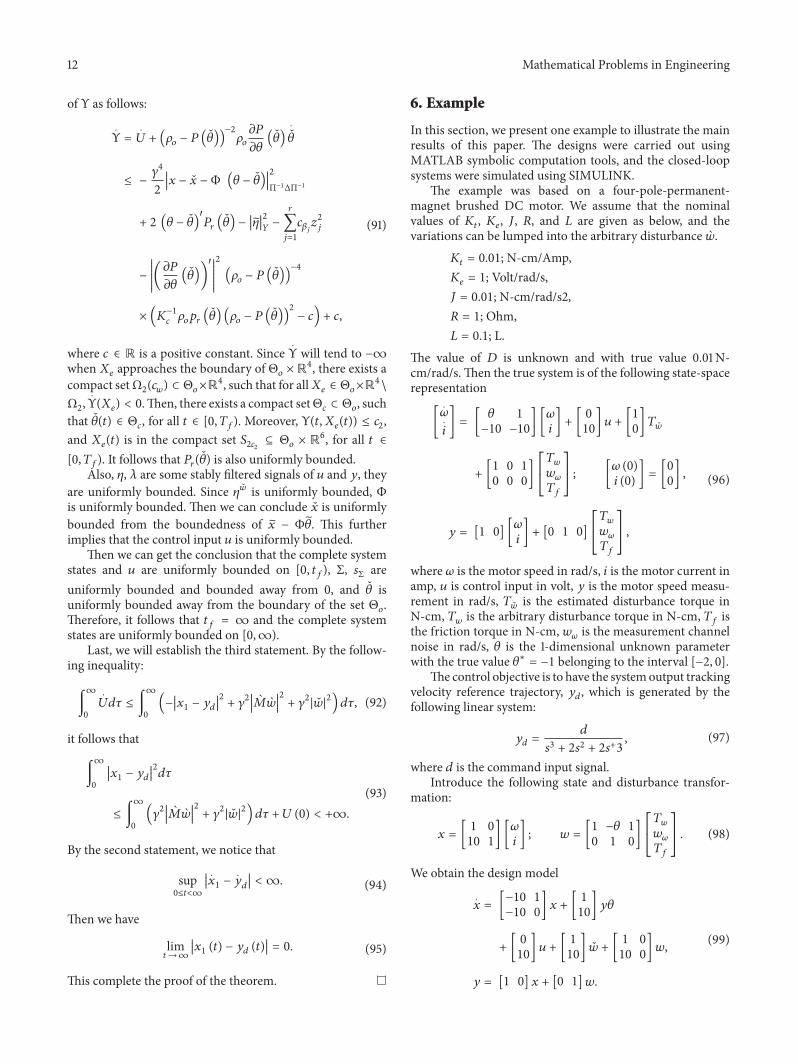
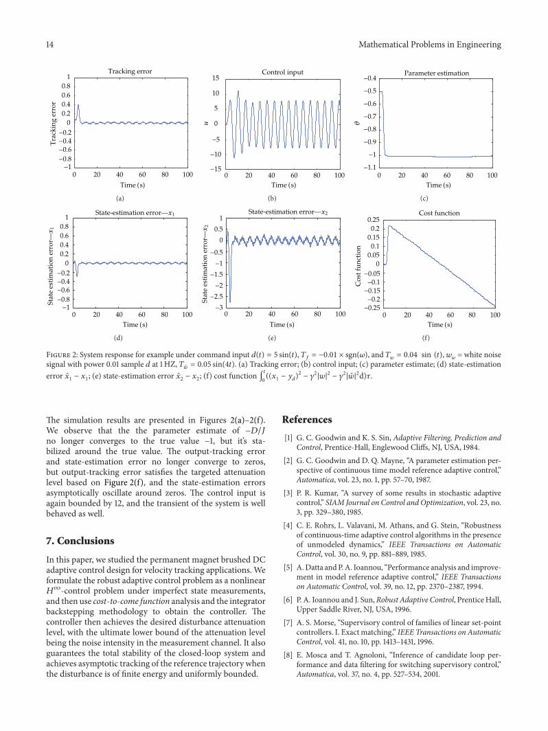applied to adaptive control problems [17ndash21] and offered apromising tool to system subjected to uncertainties

In this paper we study the adaptive control design forpermanent magnet DC motor based on worst-case analysisapproach We first model the permanent magnet DC motorservo system which is linear in all of the uncertainties Wethen formulate the robust adaptive control problem as anonlinear 119867infin-control problem under imperfect state mea-surements and apply the cost-to-come function analysis toderive the worst-case identifier and state estimator The con-trol design of the plant subsystem follows [22] and the adap-tive controller can be obtained by the integrator backstep-ping methodology The robust adaptive controller achievesasymptotic tracking if the disturbances are bounded andof finite energy and guarantees the stability of the closed-loop system with respect to the bounded disturbance inputsand the initial conditions Furthermore the close1d-loop sys-tem admits a guaranteed disturbance attenuation level withrespect to the exogenous disturbance inputs and the mea-sured disturbances where ultimate lower bound for theachievable attenuation performance level is only related tothe noise intensity in the measurement channel of the plantsystem

The balance of the paper is organized as follows InSection 2 we present the formulation of the adaptive controlproblem and discuss the general solution methodology thenwe obtain parameter identifier and state estimator usingthe cost-to-come function analysis in Section 3 In Section 4we derive the adaptive control law based on backsteppingmethod and present the main results on the robustness ofthe system in Section 5 The effectiveness of the proposedapproach is illustrated with an example in Section 6 and thepaper ends with some concluding remarks in Section 7

2 Problem Formulation

We consider a velocity-control problem of a brushed perma-nent magnet DC motor which is described by the followingdynamics

=

[[[

[

minus119863

119897

119869

119870119905

119869

minus119870

119890

119871minus119877

119871

]]]

]

119909 + [

0

1

119871

] 119906 + [

[

1

119869

0

]

]

119879+ (1a)

119910 = [1 0] 119909 + (1b)

where isin R2 is the state vector and represents load shaftangular speed and motor current respectively 119906 isin R is thescalar control input 119910 isin R is the load shaft angular speedmeasurement output 119871 isin R is the motor inductor 119877 isin R

is the armature resistance 119870119890is the back-emf constant 119870

119905is

the motor torque constant 119869 is the motor system inertia119863119897isin

R is the motor-system damping factor = [119879119908

120596

119879119891]1015840

is the arbitrary disturbance vector which is composed ofarbitrary disturbance torque 119879

119908isin R arbitrary disturbance

at the output measurement channel 120596

isin R and frictiondisturbance torque 119879

119891isin R 119879

isin R is the measured or

estimated disturbance torque In this paper we assume the

variables 119870119905 119870

119890 119869 119863

119897 119877 and 119871 are completely unknown or

partially unknownIt is easy to check that the true system is observable con-

trollable a minimal phase system and the transfer functionfrom 119906 to 119910 has relative degree 119903 = 2 And then we canfind a state diffeomorphism 119909 = and a disturbance trans-formation 119908 = by following [22] such that system (1a)and (1b) can be transformed into the following form in the 119909coordinates

119909 = 119860119909 + (11991011986021+ 119906119860

22+ 119860

23) 120579 + 119861119906 + 119863119908 + (2a)

119910 = 119862119909 + 119864119908 (2b)

where 119909 isin R2 is the state vector 119909 = [11990911199092]1015840 = 119879

120579 isin R120590 120590 isin N is the 120590-dimensional vector of unknownparameters of the true system the matrices 119860 119860

21 119860

22 119860

23

119863 119862 and 119864 are of appropriate dimensions known andhave the structure as below

119860 = [11988611

1

11988621

11988622

] 11986022

= [01times120590

11986022 0

]

119861 = [0

1198871199010

] 119862 = [1 0]

(3)

where 11986022 0

is a 120590-dimensional row vector and 1198871199010

isin R Thenthe high-frequency gain of (2a) and (2b) is 119887

0= 119887

1199010+ 119860

22 0120579

Since we consider a trajectory tracking control designproblem we make the following assumption about the refe-rence signal 119910

119889

Assumption 1 The reference trajectory 119910119889 is two times con-

tinuously differentiable Define vector119884119889= [119910

(0)

119889119910(1)

119889119910(2)

119889]1015840

and1198841198890

= [119910119889(0) 119910

(1)

119889(0)]

1015840

The signal119884119889is available for con-

trol design

To guarantee the stability of the closed-loop system andthe boundedness of the estimate of 120579 we assume there is an apriori convex compact set where the parameter vector 120579 liesin

Assumption 2 There exists a known smooth nonnegativeradially unbounded strictly convex function 119875 R120590

rarr Rsuch that the true value 120579 isin Θ = 120579 isin R120590

119875(120579) le 1 For all120579 isin Θ 119887

0= 119887

1199010+ 119860

22 0120579 gt 0

The control objective is to design a robust adaptive con-troller for system (1) such that the output 119910(119905) tracks adesired reference signal 119910

119889(119905) while rejecting the uncertain-

ties (119909(0) 120579 [0infin)

[0infin)

1198841198890 119910

(2)

119889) isin W = R2

times Θ times

C times C times R2

times C comprises the initial state the truevalues of unknown parameters unmeasured disturbancesand themeasured disturbances while all signals in the closed-loop system are uniformly bounded We make the controlobjective precise as follows



[0119905] 119879

[0119905]) and 119897

0(

0 120579

0) such that

sup(119909(0)120579119908

120596[0infin)119879119891[0infin)

119879119908[0infin)

119879[0infin)

)

119869119905

le 0 (4)

where

119869119905

= int

119905

0

((119862119909 minus 119910119889)2

+ 119897 minus 12057421003816100381610038161003816119879119908

1003816100381610038161003816

2

minus 120574210038161003816100381610038161003816119879119891

10038161003816100381610038161003816

2

minus12057421003816100381610038161003816119908120596

1003816100381610038161003816

2

minus 1205742 1003816100381610038161003816119879

1003816100381610038161003816

2

) 119889120591

minus 120574210038161003816100381610038161003816120579 minus 120579

0

10038161003816100381610038161003816

2

1198760

minus 12057421003816100381610038161003816119909 (0) minus

0

1003816100381610038161003816

2

Πminus1

0

minus 1198970

(5)









0 |119911|

119876denotes 119911

119879



119906 (119905) = 120583 (119905 119910[0119905]

[0119905]

) (6)




1003817100381710038171003817119862119909 minus 119910119889

1003817100381710038171003817

2

2(1003817100381710038171003817119879119908

1003817100381710038171003817

2

2+10038171003817100381710038171003817119879119891

10038171003817100381710038171003817

2

2

+1003817100381710038171003817119908120596

1003817100381710038171003817

2

2+1003817100381710038171003817119879

1003817100381710038171003817

2

2

+10038161003816100381610038161003816120579 minus 120579

0

10038161003816100381610038161003816

2

1198760

+1003816100381610038161003816119909 (0) minus

0

1003816100381610038161003816

2

Πminus1

0

+ 1198620)

minus1

le 1205742

(7)

where sdot2denotesL

2norm and119862

0is a constantWhen

2



lim119905rarrinfin





= [0 1]1015840


1199091015840

]1015840 we


120579 = 0

120585 = [0 0

11991011986021+ 119906119860

22+ 119860

23 119860

] 120585

+ [0119861] 119906 + [

0119863]119908 + [

0]

= 119860120585 + 119861119906 + 119863119908 +

(8a)

119910 = [0 119862] 120585 + 119864119908 = 119862120585 + 119864119908 (8b)


sup(119909(0)120579119908

[0infin)[0infin)

)isinW

119869119905

= sup119910[0infin)

[0infin)

sup(119909(0)120579119908


[0infin)

119869119905

(9)




3 Estimation Design



and [0infin)


2

119876

+ 2(120585 minus 120585)1015840



119869120574119905119891 =int

119905119891

0

(10038161003816100381610038161003816120585 minus 120585

10038161003816100381610038161003816

2

119876

+ 2(120585 minus 120585)1015840

1198972+ minus 120574

2

|119908|2

) d120591minus1205742100381610038161003816100381610038161205850

10038161003816100381610038161003816

2

1198760

(10)







Σminus1 and then


Σ = (119860 minus 1205772

119871119862)Σ + Σ(119860 minus 1205772

119871119862)1015840

+1

1205742119863119863

1015840

minus1

12057421205772

119871 1198711015840

minus Σ (1205742

1205772

1198621015840

119862 minus 1198621015840

119862 minus 119876)Σ

Σ (0) =1

1205742[119876

00

0119899times120590

Πminus1

0

]

minus1

(11a)

120585 = (119860 + Σ (1198621015840

119862 + 119876)) 120585 + 1205772

(1205742

Σ1198621015840

+ 119871) (119910 minus 119862 120585)

+ 119861119906 + minus Σ (1198621015840

119910119889+ 119876120585)

120585 (0) = [1205790

0

]

(11b)

where 120577 = 1(1198641198641015840

)12 and 119871 is defined as 119871 = [0 119871

1015840

]1015840 where

119871 = 1198631198641015840


119869119905

= minus10038161003816100381610038161003816120585 (119905) minus 120585 (119905)

10038161003816100381610038161003816

2

Σminus1(119905)

+ int

119905

0

(10038161003816100381610038161003816119862 120585 minus 119910

119889

10038161003816100381610038161003816

2

+1003816100381610038161003816120585119888

1003816100381610038161003816

2

119876

minus 1205742

120577210038161003816100381610038161003816119910 minus 119862 120585

10038161003816100381610038161003816

2

minus 120574210038161003816100381610038161003816119908 minus 119908

lowast

(119906[0120591]

119910[0120591]

[0120591]

120585[0120591]

120585[0120591]

120585[0120591]

)10038161003816100381610038161003816

2

)119889120591

(12)



119908lowast

(120591 119906[0120591]

119910[0120591]

[0120591]

120585[0120591]

120585[0120591]

120585[0120591]

)

= 1205772

1198641015840

(119910 minus 119862120585) +1

1205742(119868 minus 120577

2

1198641015840

119864)1198631015840

Σminus1

(120585 minus 120585)

(13)

We partition Σ as

Σ = [Σ Σ

12

Σ21

Σ22

] (14)



(Σ22minus Σ

21Σ

minus1

Σ12)



119876 = Σminus1

[0 00 Δ

]Σminus1

+ [120598Φ

1015840

1198621015840

(1205742

1205772

minus 1)119862Φ 00 0] (15)


120598 (120591) =

Tr (Σminus1

(120591))

119870119888

119870119888ge 120574

2 Tr (1198760) 120591 ge 0 (16)


Σ = minus (1 minus 120598) ΣΦ1015840

1198621015840

(1205742

1205772

minus 1)119862ΦΣ

Σ (0) =1

1205742119876

minus1

0

(17a)

Φ = (119860 minus 1205772

119871119862 minus1

1205742Π119862

1015840

(1205742

1205772

minus 1)119862)Φ

+ 11991011986021+ 119906119860

22+ 119860

23 Φ (0) = 0

(17b)

Π = (119860 minus 1205772

119871119862)Π+Π(119860 minus 1205772

119871119862)1015840

minusΠ1198621015840

(1205772

minus1

1205742)119862Π

+ 1198631198631015840

minus 1205772

1198711198711015840

+ 1205742

Δ Π (0) = Π0

(17c)




1

119870119888

le Σ (120591) le Σ (0) =1

1205742119876

minus1

0

1205742 Tr (119876

0) le Tr (Σminus1

(120591)) le 119870119888 forall120591 isin [0 119905]

(18)


by

119904Σ= 120574

2

1205772

(1 minus 120598) 119862ΦΦ1015840

1198621015840

119904Σ(0) = 120574

2 Tr (1198760) (19)

Then 120598(120591) = 119870minus1

119888119904minus1








2


minus1




(119860 minus 1205772

119871119862)Π + Π(119860 minus 1205772

119871119862)1015840

minus Π1198621015840

(1205772

minus1

1205742)119862Π

+ 1198631198631015840

minus 1205772

1198711198711015840

+ 1205742

Δ = 0

(20)


0






120588 = inf 119875 (120579) | 120579 isin R120590

1198871199010

+ 11986022 0

120579 = 0 (21)



Θ119900= 120579 isin R

120590

| 119875 (120579) lt 120588119900 (22)



1199010+ 119860

22 0

120579| gt 1198880

gt 0for some 119888



120597119875


120590

Θ (23)

We set 1198972= [minus(119875

119903( 120579))

1015840

0]1015840

where

119875119903( 120579) =

1198901(1minus119875(

120579))

((120597119875120597120579) ( 120579))1015840

(120588119900minus 119875 ( 120579))


119900 Θ


(24)

Then we obtain

120585 = minus Σ[(119875119903( 120579))

1015840

0]1015840

+ 119860 120585 + 119861119906 minus Σ119876120585119888

+ 1205772

(1205742

Σ1198621015840

+ 119871) (119910 minus 119862 120585) +

120585 (0) = [ 1205791015840

01015840

0]1015840

(25)

where 120585119888= 120585 minus 120585


(119860 minus 1205772

119871119862)Π + Π(119860 minus 1205772

119871119862)

minus Π1198621015840

(1205772

minus1

1205742)119862Π + 119863119863

1015840

minus 1205772

1198711198711015840

+ 1205742

Δ = 0

(26a)

Σ = minus (1 minus 120598) ΣΦ1015840

1198621015840

(1205742

1205772

minus 1)119862ΦΣ Σ (0) =1

1205742119876

minus1

0

(26b)

119904Σ= (120574

2

1205772

minus 1) (1 minus 120598) 119862ΦΦ1015840

1198621015840

119904120590(0) = 120574

2 Tr (1198760)

(26c)

120598 =1

119870119888119904Σ

(26d)

119860119891= 119860 minus 120577

2

119871119862 minus Π1198621015840

119862(1205772

minus1

1205742) (26e)

Φ = 119860119891Φ + 119910119860

21+ 119906119860

22+ 119860

23 Φ (0) = 0 (26f)

120579 = minus Σ119875119903( 120579) minus ΣΦ

1015840

1198621015840

(119910119889minus 119862)


] 119876120585119888+120574

2

1205772

ΣΦ1015840

1198621015840

(119910 minus 119862) 120579 (0)= 1205790

(26g)

= minus ΦΣ119875119903( 120579) + 119860 minus (

1

1205742Π + ΦΣΦ

1015840

)1198621015840

(119910119889minus 119862)

minus [ΦΣ1

1205742Π + ΦΣΦ

1015840

]119876120585119888

+ (11991011986021+ 119906119860

22+ 119860

23) 120579

+ 1205772

(Π1198621015840

+ 1205742

ΦΣΦ1015840

1198621015840

+ 119871)

times (119910 minus 119862) + + 119861119906 (0) = 0





119891= [119860

11989111990121199012] (27)


119891 119901

2)



120578 = 119860119891120578 + 119901

2119910 120578 (0) = 0 (28a)

120582 = 119860119891120582 + 119901

2119906 120582 (0) = 0 (28b)

120578

= 119860119891120578

+ 1199012 120578

(0) = 0 (28c)

Φ = [119860119891120578 120578]119872

minus1

119891119860

21+ [119860

119891120582 120582]119872

minus1

119891119860

22

+ [119860119891120578

120578

]119872minus1

119891119860

23

(28d)



119882(119905 120585 (119905) 120585 (119905) Σ (119905))

=10038161003816100381610038161003816120585 (119905) minus 120585 (119905)

10038161003816100381610038161003816

2

Σ

minus1

(119905)

=10038161003816100381610038161003816120579 minus 120579 (119905)

10038161003816100381610038161003816

2

Σminus1

(119905)


10038161003816100381610038161003816

2

Πminus1

(29)


119882 = minus1003816100381610038161003816119862119909 minus 119910

119889

1003816100381610038161003816

2


10038161003816100381610038161003816

2

Πminus1

ΔΠminus1

minus 120598 (1205742

1205772

minus 1)10038161003816100381610038161003816120579 minus 120579

10038161003816100381610038161003816

2

Φ10158401198621015840119862Φ

+ 1205742

|119908|2

+1003816100381610038161003816119862 minus 119910

119889

1003816100381610038161003816

2

+1003816100381610038161003816120585119888

1003816100381610038161003816

2

119876

minus 1205742

12057721003816100381610038161003816119910 minus 119862

1003816100381610038161003816

2

minus 120574210038161003816100381610038161003816119908 minus 119908

lowast

(119905 119906[0119905]

119910[0119905]

[0119905]

120585[0119905]

120585[0119905]

120585[0119905]

)10038161003816100381610038161003816

2

+ 2(120579 minus 120579)1015840

119875119903( 120579)

(30)




119869119905

= 119869119905

+119882(0) minus119882 (119905) + int

119905

0

119882119889120591

= minus10038161003816100381610038161003816120579 minus 120579 (119905)

10038161003816100381610038161003816

2

Σminus1

(119905)


10038161003816100381610038161003816

2

Πminus1

+ int

119905

0

(1003816100381610038161003816119862 minus 119910

119889

1003816100381610038161003816

2

+1003816100381610038161003816120585119888

1003816100381610038161003816

2

119876

minus 1205742

12057721003816100381610038161003816119910 minus 119862

1003816100381610038161003816

2

minus 120574210038161003816100381610038161003816119908 minus 119908

lowast

times (120591 119906[0120591]

119910[0120591]

[0120591]

120585[0120591]

120585[0120591]

120585[0120591]

)10038161003816100381610038161003816

2

+ minus 1205742

||2

) 119889120591

(31)


4 Control Design




119869119905


[0infin)

int

119905

0

(1003816100381610038161003816119862 minus 119910

119889

1003816100381610038161003816

2

+1003816100381610038161003816120585119888

1003816100381610038161003816

2

119876

minus 1205742

12057721003816100381610038161003816119910 minus 119862

1003816100381610038161003816

2

+ minus 1205742

||2

) 119889120591 minus 1198970

(32)

where function (120591 119910[0120591]

[0120591]


[0120591]




119907 = [120577 (119910 minus 119862)

] (33)

Then we have

120578 = 119860119891120578 + 119901

2119862 + 119901

2(1198901015840

21119907

120577) (34)

120579 = minus Σ119875119903( 120579) minus ΣΦ

1015840

1198621015840

(119910119889minus 119862)


] 119876120585119888+ 120574

2

ΣΦ1015840

1198621015840

1205771198901015840

21119907

(35)

= 119860 minus (1

1205742Π + ΦΣΦ

1015840

)1198621015840

(119910119889minus 119862) + 119860

21

120579119862

minus ΦΣ119875119903( 120579) minus [ΦΣ

1

1205742Π + ΦΣΦ

1015840

]119876120585119888+ 119861119906

+ 11986022

120579119906 + ((120577minus2

11986021

120579 + Π1198621015840

+ 1205742

ΦΣΦ1015840

1198621015840

+ 119871) 1205771198901015840

21

+11986023

1205791198901015840

22+ [0

119899times1] ) 119907

(36)

119882 = minus1003816100381610038161003816119862119909 minus 119910

119889

1003816100381610038161003816

2


10038161003816100381610038161003816

2

Πminus1

ΔΠminus1

minus 120598 (1205742

1205772

minus 1)10038161003816100381610038161003816120579 minus 120579

10038161003816100381610038161003816

2

Φ10158401198621015840119862Φ

+1003816100381610038161003816119862 minus 119910

119889

1003816100381610038161003816

2

+1003816100381610038161003816120585119888

1003816100381610038161003816

2

119876

+ 2(120579 minus 120579)1015840

119875119903( 120579)

+ 1205742

||2

+ 1205742

|119908|2

minus 1205742

|119907|2

minus 120574210038161003816100381610038161003816119908 minus 119908

lowast

(119905 119906[0119905]

119910[0119905]

[0119905]

120585[0119905]

120585[0119905]

120585[0119905]

)10038161003816100381610038161003816

2

(37)






Φ = 119860119891Φ + 119910119860

21+ 119906119860

22+ 119860

23 Φ (0) = 0 (38)


Φ = Φ119906

+ Φ119910

+ Φ

(39a)

Φ119910

= [119860119891120578 120578]119872

minus1

119891119860

21= [

1205781015840

1198791

1205781015840

1198792

] (39b)

Φ119906

= 119860119891Φ

119906

+ 11990611986022 Φ

119906

(0) = 0 (39c)

Φ

= 119860119891Φ

+ 11986023 Φ

(0) = 0 (39d)


depending on119860119891119872

119891 and119860



= [Φ1199061015840

1Φ

1199061015840

2]

1015840

andΦ

= [Φ1015840

1Φ

1015840

2]1015840

Then 119862Φ119910

= 1205781015840

1198791 119862Φ119906

= Φ119906

1 and 119862Φ

= Φ

1


119904Σ= (120574

2

1205772

minus 1) (1 minus 120598) (1205781015840

1198791+ Φ

119906

1+ Φ

1)

times (1205781015840

1198791+ Φ

119906

1+ Φ

1)1015840

(40a)

120598 =1

119870119888119904Σ

(40b)

Σ = minus (1 minus 120598) Σ(1205781015840

1198791+ Φ

119906

1+ Φ

1)1015840

times (1205742

1205772

minus 1) (1205781015840

1198791+ Φ

119906

1+ Φ

1) Σ

(40c)

120579 = 120575 (119910119889minus

1 120578 Φ

1 Φ

119906

1 120579

997888rarrΣ)

+ 120593(120578997888rarrΦ

997888rarrΦ

119906

997888rarrΣ)119876120585

119888+ 120581 (120578Φ

1 Φ

119906

1997888rarrΣ) 119907

(40d)

120578 = 119860119891120578 + 119901

21+ 119901

2(1198901015840

21119907

120577) (40e)

1=

2+ 119891

1(119910

119889minus

1

1 120579 120578 Φ

1 Φ

119906

1997888rarrΣ)

+ 9848581(120578

997888rarrΦ

997888rarrΦ

119906

997888rarrΣ)119876120585

119888

+ ℎ1( 120579 120578 Φ

1 Φ

119906

1997888rarrΣ) 119907

(40f)

2= 119886

222+ (119887

1199010+ 119860

220

120579) 119906

+ 1198912(119910

119889minus

1

1

2 120579 120578 Φ

1 Φ

2 Φ

119906

1 Φ

119906

2997888rarrΣ)

+ 9848582(120578

997888rarrΦ

997888rarrΦ

119906

997888rarrΣ)119876120585

119888

+ ℎ2( 120579 120578 Φ

1 Φ

2 Φ

119906

1 Φ

119906

2997888rarrΣ) 119907

(40g)

Φ119906

1= 120595

1(Φ

119906

1) + Φ

119906

2 (40h)

Φ

1= 120603

1(Φ

1) + Φ

2+ 119890

1015840

21119860

231198901015840

22119907 (40i)


2are smooth as


1 984858

2 ℎ

1 ℎ

2

1205951 and 120603


119906

1 Φ119906

2 Φ

1 and Φ

2



119888 which









120578119889= 119860

119891120578119889+ 119901

2119910119889 120578

119889(0) = 0

2 times 1 (41)


dynamics

120578 = 119860119891120578 + 119901

2(1198901015840

21119907

120577) + 119901

2(

1minus 119910

119889) (42)




1198601015840

119891119885 + 119885119860

119891+

1

12057421205772119885119901

21199011015840

2119885 + 119884 = 0 (43)



1198810(120578) =

10038161003816100381610038161205781003816100381610038161003816

2

119885 (44)


1198810= minus

10038161003816100381610038161205781003816100381610038161003816

2

119884+ 120574

2

|119907|2

minus 12057421003816100381610038161003816119907 minus 120584

0

1003816100381610038161003816

2

+ 21205781015840

119885119901119899(

1minus 119910

119889) (45)


where

1205840(120578) =

1

1205742120577119890211199011015840

2119885120578 (46)


1= 119910

119889 (47)





1199111=

1minus 119910

119889 (48)


119889


1199111= 119891

1(119911

1 119910

119889 120579 120578 Φ

1 Φ

119906

1997888rarrΣ) +

2minus 119910

(1)

119889

+ 9848581(120578

997888rarrΦ

997888rarrΦ

119906

997888rarrΣ)119876120585

119888+ ℎ

1( 120579 120578 Φ

1 Φ

119906

1997888rarrΣ) 119907

(49)


1198911(119911

1 119910

119889 120579 120578 Φ

1 Φ

119906

1997888rarrΣ)

= 1198911(119910

119889minus

1

1 120579 120578 Φ

1 Φ

119906

1997888rarrΣ)

(50)


1198811= 119881

0+1

21199112

1(51)


1198811= minus

10038161003816100381610038161205781003816100381610038161003816

2

119884+ 120574

2

|119907|2

minus 12057421003816100381610038161003816119907 minus 120584

0

1003816100381610038161003816

2

+ 21205781198851199011198991199111

+ 1199111(

2minus 119910

(1)

119889+ 119891

1+ 984858

1119876120585

119888+ ℎ

1119907)

= minus1199112

1minus10038161003816100381610038161205781003816100381610038161003816

2

119884minus 120573

11199112

1+ 119911

11199112+ 120589

1015840

1119876120585

119888

+ 1205742

|119907|2

minus 12057421003816100381610038161003816119907 minus 120584

1

1003816100381610038161003816

2

(52)

where

1199112=

2minus 119910

(1)

119889minus 120572

1 (53a)

1205841(119911

1 120579 120578 120578 Φ

1 Φ

119906

1997888rarrΣ) = 120584

0+

1

21205742ℎ1015840

11199111 (53b)

1205721(119911

1 119910

119889 120579 120578 120578 Φ

1 Φ

119906

1997888rarrΣ 119904) = minus 119911

1minus 120573

11199111minus 2119901

1015840

119899119885120578


11205840minus

1

41205742ℎ1ℎ1015840

11199111

(53c)

1205731(119911

1 119910

119889 120579 120578 120578 Φ

1 Φ

119906

1997888rarrΣ 119904) ge 119888

1205731

gt 0 (53d)

1205891(119911

1 119910

119889 120578 120578 Φ

1 Φ

119906

997888rarrΣ) = 984858

1015840

11199111 (53e)

where 1198881205731


1is




2= 119910

(1)

119889+ 120572

1 (54)


supply rate

minus10038161003816100381610038161

minus 119910119889

1003816100381610038161003816

2

minus10038161003816100381610038161205781003816100381610038161003816

2

119884minus 120573

11199112

1+ 120574

2

1199072

(55)



2 which is given by

1199112= 119886

222+ (119887

1199010+ 119860

220

120579) 119906

minus 119910(2)

119889+ 120594

21+ 2120574

2

12059422119907 + 120594

23119876120585

119888

(56)

where 12059421 120594

22 and 120594


12059421

= 1198912minus120597120572

1

1205971

(1198911+

2) minus

1205971205721

120597119910119889

119910(1)

119889

minus120597120572

1

120597 120579

120575 minus120597120572

1

120597120578(119860

119891120578 + 119901

21199111)

minus120597120572

1

120597120578(119860

119891120578 + 119901

21) minus

1205971205721

120597Φ

1

(Φ

2+ 120603

1)1015840

minus120597120572

1

120597Φ119906

1

(Φ119906

2+ 120595

1)1015840

minus120597120572

1

120597997888rarrΣ

(120598 minus 1)

times

997888997888997888997888997888997888997888997888997888997888997888997888997888997888997888997888997888997888997888997888997888997888997888997888997888997888997888997888997888997888997888997888997888997888997888997888997888997888997888997888997888997888997888997888997888997888997888rarr

(Σ(1205781015840

1198791+Φ

1+ Φ

119906

1)1015840

(1205742

1205772

minus1) (1205781015840

1198791+Φ

1+Φ

119906

1) Σ)

minus120597120572

1

120597119904Σ

(1205742

1205772

minus 1) (1 minus 120598) (1205781015840

1198791+ Φ

1+ Φ

119906

1)

times (1205781015840

1198791+ Φ

1+ Φ

119906

1)1015840

12059422

=1

21205742(ℎ

2minus120597120572

1

1205971

ℎ1minus120597120572

1

120597 120579

120581 minus120597120572

1

120597120578

11990121198901015840

21

120577

minus120597120572

1

120597120578

11990121198901015840

21

120577minus

1205971205721

120597Φ

1

1198601015840

23119890221198901015840

22)

12059423

= 9848582minus120597120572

1

1205971

9848581minus120597120572

1

120597 120579

120593

(57)


1198812= 119881

1+1

21199112

2 (58)


1198812= minus119911

2

1minus10038161003816100381610038161205781003816100381610038161003816

2

119884minus

2

sum

119895=1

1205731198951199112

119895+ 120574

2

|119907|2

minus 12057421003816100381610038161003816119907 minus 120584

2

1003816100381610038161003816

2

+ 1205891015840

2119876120585

119888

(59)



119906 = 120583 (1199111 119911

2

1

2 119910

119889 119910

(1)

119889

120579 120578 120578 Φ

1 Φ

2 Φ

119906

1 Φ

119906

119903

997888rarrΣ 119904

Σ)

= minus1

1198871199010

+ 119860220

120579

(119886222minus 119910

(2)

119889minus 120572

2)

(60)

where

1205722= minus 120594

21minus 2120574

2

120594222

minus 21205742

120594221

1198901015840

211205841

minus 1205742

1205942

2211199112minus 120573

21199112minus 119911

1

(61)

1205842= 120584

1+ 119890

21120594221

1199112 (62)

where 12059422

= [120594221

120594222


22

12059423 120584

2 and 120589


119900



119880 = 1198812+119882 =

10038161003816100381610038161003816120579 minus 120579

10038161003816100381610038161003816

2

Σminus1+ 120574


10038161003816100381610038161003816

2

Πminus1

+10038161003816100381610038161205781003816100381610038161003816

2

119885+1

2

2

sum

119895=1

(119895minus 119910

(119895minus1)

119889minus 120572

119895minus1)2

(63)



119880 = minus1003816100381610038161003816119862119909 minus 119910

119889

1003816100381610038161003816

2


10038161003816100381610038161003816

2

Πminus1

ΔΠminus1

minus 120598 (1205742

1205772

minus 1)10038161003816100381610038161003816120579 minus 120579

10038161003816100381610038161003816

2

Φ10158401198621015840119862Φ

+ 2(120579 minus 120579)1015840

119875119903( 120579) +

10038161003816100381610038161205851198881003816100381610038161003816

2

119876

+ 1205891015840

119903119876120585

119888minus10038161003816100381610038161205781003816100381610038161003816

2

119884

minus

2

sum

119895=1

1205731198951199112

119895+ 120574

2

|119908|2

+ 1205742

||2

minus 120574210038161003816100381610038161003816119908 minus 119908

lowast

(119905 119906[0119905]

119910[0119905]

[0119905]

120585[0119905]

120585[0119905]

120585[0119905]

)10038161003816100381610038161003816

2

minus 12057421003816100381610038161003816119907 minus 120584

2

1003816100381610038161003816

2

= minus1003816100381610038161003816119862119909 minus 119910

119889

1003816100381610038161003816

2


10038161003816100381610038161003816

2

Πminus1

ΔΠminus1

minus 120598 (1205742

1205772

minus 1)10038161003816100381610038161003816120579 minus 120579

10038161003816100381610038161003816

2

Φ10158401198621015840119862Φ

+ 2(120579 minus 120579)1015840

119875119903( 120579) +

1003816100381610038161003816100381610038161003816120585119888+1

21205892

1003816100381610038161003816100381610038161003816

2

119876

minus1

4

100381610038161003816100381612058921003816100381610038161003816

2

119876

minus10038161003816100381610038161205781003816100381610038161003816

2

119884minus

2

sum

119895=1

1205731198951199112

119895+ 120574

2

|119908|2

+ 1205742

||2

minus 120574210038161003816100381610038161003816119908 minus 119908

lowast

(119905 119906[0119905]

119910[0119905]

[0119905]

120585[0119905]

120585[0119905]

120585[0119905]

)10038161003816100381610038161003816

2

minus 12057421003816100381610038161003816119907 minus 120584

2

1003816100381610038161003816

2

(64)


120585lowast

119888= minus

1

21205892lArrrArr 120585

lowast

= 120585 minus1

21205892 (65)


minus10038161003816100381610038161199091

minus 119910119889

1003816100381610038161003816

2

+ 1205742

|119908|2

+ 1205742

||2

(66)


119908opt = 1205771198641015840

1198901015840

211205842+

1

1205742(119868 minus 120577

2

1198641015840

119864)1198631015840

Σminus1

(120585 minus 120585)

+ 1205772

1198641015840

119862 ( minus 119909)

(67)

opt = 119890221205842 (68)

5 Main Result



119883 = 119865 (119883 119910(2)

119889) + 119866 (119883)119908 + 119866

(119883) (69)


119883 = [1205791015840

1199091015840

119904Σ

1205791015840

1015840

1205781015840

1205781015840

1198891205781015840

997888rarrΦ

119906

1015840 larr997888Σ

1015840

119910119889

119910(1)

119889

]

1015840

(70)


119900119865


0isin D

0= 119883


Θ 1205790isin Θ Σ(0) = 120574

minus2

119876minus1

0gt 0Tr((Σ(0))minus1) le 119870

119888 119904

Σ(0) =

1205742 Tr(119876

0)


119889isin R

120597119880

120597119883(119883) 119865 (119883 119910

(2)

119889) +

1

41205742

120597119880

120597119883(119883) [119866 (119883) 119866

119908(119883)]

sdot [119866 (119883) 119866119908(119883)]

1015840

(120597119880

120597119883(119883))

1015840

+ 119876 (119883 119910(2)

119889) = 0

(71)



119876(119883 119910(2)

119889) =

100381610038161003816100381611990911minus 119910

119889

1003816100381610038161003816

2

+(10038161003816100381610038161003816120585 minus 120585

10038161003816100381610038161003816

2

119876

+119875119903( 120579)

10038161003816100381610038161205781003816100381610038161003816

2

119884minus2(120579 minus 120579)

1015840

times119875119903( 120579)+

2

sum

119895=1

1205731198951199112

119895+1

4

100381610038161003816100381612058921003816100381610038161003816

2

119876)

(72)




[0infin)

[0infin)

1198841198890 119910

(2)

119889) isin W

(2) Given a 119888119908




(119909(0) 120579 [0infin)

[0infin)

119884119889) with

|119909 (0)| le 119888119908 | (119905)| le 119888

119908 | (119905)| le 119888

119908

1003816100381610038161003816119884119889(119905)


(73)


119889


|119909 (119905)| le 119888119888 | (119905)| le 119888

119888 120579 (119905) isin Θ

119888

1003816100381610038161003816120578 (119905)1003816100381610038161003816 le 119888

119888

1003816100381610038161003816120578119889 (119905)1003816100381610038161003816 le 119888

119888 |120582 (119905)| le 119888

119888

1003816100381610038161003816100381612057810038161003816100381610038161003816le 119888

119888

1

119870119888

119868 le Σ (119905) le1

1205742119876

minus1

0

1

119870119888

le 119904Σ(119905) le

1

1205742 Tr (1198760)

(74)


[0infin)

119884119889[0infin)

) with [0infin)

isin L2capL

infin

[0infin)isin L

2capL

infin

and 119884119889[0infin)


1


is

lim119905rarrinfin

(1199091(119905) minus 119910

119889(119905)) = 0 (75)


1198970(

0 120579

0) = 119881

2(0) =

1

2

2

sum

119895=1

1199112

119895(0)

119897 (120591 120579 119909 119910[0119905]

[0119905]

) =10038161003816100381610038161003816120585 minus 120585

10038161003816100381610038161003816

2

119876

minus 2(120579 minus 120579)1015840

119875119903( 120579)

+1

4

100381610038161003816100381612058921003816100381610038161003816

2

119876

+10038161003816100381610038161205781003816100381610038161003816

2

119884+

2

sum

119895=1

1205731198951199112

119895


10038161003816100381610038161003816

2

Πminus1

ΔΠminus1

+ 120598 (1205742

1205772

minus 1)10038161003816100381610038161003816120579 minus 120579

10038161003816100381610038161003816

2

Φ10158401198621015840119862Φ

minus 2(120579 minus 120579)1015840

119875119903( 120579) +

1

4

100381610038161003816100381612058921003816100381610038161003816

2

119876

+10038161003816100381610038161205781003816100381610038161003816

2

119884+

2

sum

119895=1

1205731198951199112

119895

(76)

then we have

119869119905

= 119869119905

+ int

119905

0

119880119889120591 minus 119880 (119905) + 119880 (0)

le minus119880 (119905) le 0

(77)

It follows thatsup

(119909(0)120579119908[0infin)

[0infin)

)isinW

119869119905

le 0 (78)


119891)



Fix 119888119908

ge 0 and 119888119889


0 120579

[0infin)

[0infin) 119884


10038161003816100381610038161199090

1003816100381610038161003816 le 119888119908 | (119905)| le 119888

119908 | (119905)| le 119888

119908

1003816100381610038161003816119884119889(119905)

1003816100381610038161003816 le 119888119889


(79)





119883119890= [ 120579

1015840

(119909 minus Φ120579)1015840

1205781015840

11991111199112]

1015840

(80)


119880119872(119883

119890) = 119870

119888

1003816100381610038161003816100381612057910038161003816100381610038161003816

2

+ 120574210038161003816100381610038161003816119909 minus Φ120579

10038161003816100381610038161003816

2

Πminus1+10038161003816100381610038161205781003816100381610038161003816

2

119885+

2

sum

119895=1

1

21199112

119895

119880119898(119883

119890) = 120574

21003816100381610038161003816100381612057910038161003816100381610038161003816

2

1198760

+ 120574210038161003816100381610038161003816119909 minus Φ120579

10038161003816100381610038161003816

2

Πminus1+10038161003816100381610038161205781003816100381610038161003816

2

119885+

2

sum

119895=1

1

21199112

119895

(81)


then we have

119880119898(119883

119890)le119880 (119905 119883

119890)le119880

119872(119883

119890) forall (119905 119883

119890)isin [0 119879

119891)timesR

6+120590

(82)

Since119880119898(119883



= 119883119890isin R6+120590

|

119880119898(119883


119908 and



119880 le minus1205744

2


10038161003816100381610038161003816

2

Πminus1

ΔΠminus1+ 2 (120579 minus 120579)

1015840

119875119903( 120579)

minus10038161003816100381610038161205781003816100381610038161003816

2

119884minus

2

sum

119894=1

1205731198941199112

119894+ 120574

21003817100381710038171003817100381710038171003817100381710038171003817

2

2

1198882

119908+ 120574

2

1198882

119908

(83)

Since minus(1205744


Πminus1


2

119884+2 (120579 minus 120579)

1015840

119875119903( 120579)minus

sum2

119895=11205731198951199112




1(119888

119908) sub Θ

119900timesR6

such that

119880 lt 0 for for all 119883119890


Ω1 Then

119880(119905 119883119890(119905)) le 119888

1 and 119883


11198881



119890is uniformly


2are uniformly


119889 we have 120578

119889is uniformly



119871

120578 = 119860119891120578 + 119901

2119910

120578119871= 119879

119871120578

(84)




119910

+ Φ119906

+ Φ Since Φ

119910 and Φ are



Φ119906

= Φ119906119904

+ 120582119887119860

22 0

120582119887= [

1205821198871

1205821198872

]

120582119887= 119860

119891120582119887+ 119890

22119906 120582

119887(0) = 0

2times1

Φ119906119904

= [Φ

1199061199041

Φ1199061199042

]

Φ119906119904

= 119860119891Φ

119906119904

Φ119906119904

(0) = Φ119906 0

(85)




1199091minus Φ

1199061199041120579 minus 120582

1198871119860

22 0120579 minus Φ

1120579 minus 120578

10158401198791

120579

(86)


1198871119860



Φ and 120578 Since1199111=

1minus 119910

119889 and 119911

1 119910


1is


119891= 119860 minus 120577

2

119871119862 minus Π1198621015840

119862(1205772

minus 120574minus2

) and 1198870=

1198871199010

+ 11986022 0


01205821198871by

119909 minus 1198870

120582119887= 119860

119891(119909 minus 119887

0120582119887) + 119860

21120579119910 + 119863 + 119860

23120579

+ (1205772

119871 + Π1198621015840

(1205772

minus1

1205742)) (119910 minus 119864) +

1199091minus 119887

01205821198871

= 119862 (119909 minus 1198870120582119887)

(87)





01205821198871


1minus120582

1198871(119887

1199010+119860

212 0







01205821198871 and are



0120582119887since 119860






Θ119900such that 120579(119905) isin Θ

119888 for all 119905 isin [0 119879


function

Υ = 119880 + (120588119900minus 119875 ( 120579))

minus1

119875 ( 120579) (88)






Υ119872

= 119880119872(119883

119890) + (120588

119900minus 119875 ( 120579))

minus1

119875 ( 120579)

Υ119898= 119880

119898(119883

119890) + (120588

119900minus 119875 ( 120579))

minus1

119875 ( 120579)

(89)


Υ119898(119883

119890) le Υ (119905 119883

119890) le Υ

119872(119883

119890)

forall (119905 119883119890) isin [0 119879

119891) times Θ

119900timesR

6

(90)


= 119883119890isin Θ

119900times R6

| Υ119898(119883

119890) le 120572



of Υ as follows

Υ =

119880 + (120588119900minus 119875 ( 120579))

minus2

120588119900

120597119875

120597120579( 120579)

120579

le minus1205744

2


10038161003816100381610038161003816

2

Πminus1

ΔΠminus1

+ 2 (120579 minus 120579)1015840

119875119903( 120579) minus

10038161003816100381610038161205781003816100381610038161003816

2

119884minus

119903

sum

119895=1

119888120573119895

1199112

119895

minus

100381610038161003816100381610038161003816100381610038161003816

(120597119875

120597120579( 120579))

1015840100381610038161003816100381610038161003816100381610038161003816

2

(120588119900minus 119875 ( 120579))

minus4

times (119870minus1

119888120588119900119901119903( 120579) (120588

119900minus 119875 ( 120579))

2

minus 119888) + 119888

(91)






119908) sub Θ


119890isin Θ

119900timesR4

Ω2


119888sub Θ

119900 such


119891) Moreover Υ(119905 119883

119890(119905)) le 119888

2


21198882


[0 119879119891) It follows that 119875





119891) Σ 119904

Σare


119900



ing inequality

int

infin

0

119880119889120591 le int

infin

0

(minus10038161003816100381610038161199091

minus 119910119889

1003816100381610038161003816

2

+ 120574210038161003816100381610038161003816

10038161003816100381610038161003816

2

+ 1205742

||2

) 119889120591 (92)

it follows that

int

infin

0

10038161003816100381610038161199091minus 119910

119889

1003816100381610038161003816

2

119889120591

le int

infin

0

(120574210038161003816100381610038161003816

10038161003816100381610038161003816

2

+ 1205742

||2

) 119889120591 + 119880 (0) lt +infin

(93)


sup0le119905ltinfin

1003816100381610038161003816

1199091minus

119910119889

1003816100381610038161003816 lt infin (94)

Then we have

lim119905rarrinfin

10038161003816100381610038161199091(119905) minus 119910

119889(119905)

1003816100381610038161003816 = 0 (95)


6 Example



119905 119870



119905= 001 N-cmAmp

119870119890= 1 Voltrads

119869 = 001 N-cmrads2119877 = 1 Ohm119871 = 01 L


[

120596

119894] = [

120579 1

minus10 minus10] [

120596

119894] + [

0

10] 119906 + [

1

0]119879

+ [1 0 1

0 0 0][

[

119879119908

119908120596

119879119891

]

]

[120596 (0)

119894 (0)] = [

0

0]

119910 = [1 0] [120596

119894] + [0 1 0] [

[

119879119908

119908120596

119879119891

]

]

(96)




119891is






119910119889=

119889

1199043 + 21199042 + 2119904+3 (97)


mation

119909 = [1 0

10 1] [

120596

119894] 119908 = [

1 minus120579 1

0 1 0][

[

119879119908

119908120596

119879119891

]

]

(98)


119909 = [minus10 1

minus10 0] 119909 + [

1

10] 119910120579

+ [0

10] 119906 + [

1

10] + [

1 0

10 0]119908

119910 = [1 0] 119909 + [0 1]119908

(99)


0 5 10 15 20 25 30minus1


002040608

1Tracking error

Tra

ckin

g er

ror

Time (s)

(a)

0 5 10 15 20 25 30minus15

minus10

minus5

0

5

10

15Control input

u

Time (s)

(b)

0

0

5 10 15 20 25 30minus2




Time (s)

θ

(c)


000501

Time (s)


Stat

e es

tim

atio

n er

rormdash

x1

(d)

0 5 10 15 20 25 30minus4

minus35minus3

minus25minus2

minus15minus1

minus050

051

Time (s)


ate

esti

mat

ion

erro

rmdashx

2

(e)

0 5 10 15 20 25 300

005

01

015

02

025Cost function

Cos

t fun

ctio

n

Time (s)

(f)


119908= 0 119908

120596= 0 and 119879




2minus 119909


119905

0

((1199091minus 119910

119889)2

minus

1205742

|119908|2

minus 1205742

||2d)120591


119875 (120579) = (120579 + 1)2

(100)


0= [

01

05] 120579

0= minus05

1198760= 1 119870

119888= 100 Δ = [

1 0

0 1]

1205731= 120573

2= 05 119884 = [

1592262 minus170150

minus170150 18786]

(101)

Then we obtain

119860119891= [

minus102993 10000

minus122882 0] 119885 = [

88506 minus09393

minus09393 01229]

Π = [05987 45764

45764 431208]

(102)


119879119891= 0 N-cm

119879119908= 0 N-cm

119908120596= 0 rads

119879= 0 N-cm




119879119908= 004 sin (119905) N-cm


1 HZ rads119879= 005 sin (4119905) N-cm


0 20 40 60 80 100

Time (s)


002040608

1Tracking error

Tra

ckin

g er

ror

(a)

0 20 40 60 80 100

Control input

minus15

minus10

minus5

0

5

10

15

u

Time (s)

(b)

0 20 40 60 80 100minus11

minus1

minus09

minus08

minus07

minus06

minus05

minus04

Time (s)

θ


(c)

0 20 40 60 80 100Time (s)


002040608


Stat

e es

tim

atio

n er

rormdash

x1

(d)

0 20 40 60 80 100minus3

minus25

minus2

minus15

minus1

minus05

0

05

1

Time (s)


Stat

e es

tim

atio

n er

rormdash

x2

(e)


minus0050

00501

01502

025

Time (s)

Cost function

Cos

t fun

ctio

n

(f)


119908= 004 sin (119905) 119908

120596= white noise


error 1minus 119909


2minus 119909


119905

0

((1199091minus 119910

119889)2

minus 1205742

|119908|2

minus 1205742

||2d)120591



7 Conclusions



References














infin





















Volume 2014




Journal of











Journal of


Function Spaces






Algebra











[0119905] 119879

[0119905]) and 119897

0(

0 120579

0) such that

sup(119909(0)120579119908

120596[0infin)119879119891[0infin)

119879119908[0infin)

119879[0infin)

)

119869119905

le 0 (4)

where

119869119905

= int

119905

0

((119862119909 minus 119910119889)2

+ 119897 minus 12057421003816100381610038161003816119879119908

1003816100381610038161003816

2

minus 120574210038161003816100381610038161003816119879119891

10038161003816100381610038161003816

2

minus12057421003816100381610038161003816119908120596

1003816100381610038161003816

2

minus 1205742 1003816100381610038161003816119879

1003816100381610038161003816

2

) 119889120591

minus 120574210038161003816100381610038161003816120579 minus 120579

0

10038161003816100381610038161003816

2

1198760

minus 12057421003816100381610038161003816119909 (0) minus

0

1003816100381610038161003816

2

Πminus1

0

minus 1198970

(5)









0 |119911|

119876denotes 119911

119879



119906 (119905) = 120583 (119905 119910[0119905]

[0119905]

) (6)




1003817100381710038171003817119862119909 minus 119910119889

1003817100381710038171003817

2

2(1003817100381710038171003817119879119908

1003817100381710038171003817

2

2+10038171003817100381710038171003817119879119891

10038171003817100381710038171003817

2

2

+1003817100381710038171003817119908120596

1003817100381710038171003817

2

2+1003817100381710038171003817119879

1003817100381710038171003817

2

2

+10038161003816100381610038161003816120579 minus 120579

0

10038161003816100381610038161003816

2

1198760

+1003816100381610038161003816119909 (0) minus

0

1003816100381610038161003816

2

Πminus1

0

+ 1198620)

minus1

le 1205742

(7)

where sdot2denotesL

2norm and119862

0is a constantWhen

2



lim119905rarrinfin





= [0 1]1015840


1199091015840

]1015840 we


120579 = 0

120585 = [0 0

11991011986021+ 119906119860

22+ 119860

23 119860

] 120585

+ [0119861] 119906 + [

0119863]119908 + [

0]

= 119860120585 + 119861119906 + 119863119908 +

(8a)

119910 = [0 119862] 120585 + 119864119908 = 119862120585 + 119864119908 (8b)


sup(119909(0)120579119908

[0infin)[0infin)

)isinW

119869119905

= sup119910[0infin)

[0infin)

sup(119909(0)120579119908


[0infin)

119869119905

(9)




3 Estimation Design



and [0infin)


2

119876

+ 2(120585 minus 120585)1015840



119869120574119905119891 =int

119905119891

0

(10038161003816100381610038161003816120585 minus 120585

10038161003816100381610038161003816

2

119876

+ 2(120585 minus 120585)1015840

1198972+ minus 120574

2

|119908|2

) d120591minus1205742100381610038161003816100381610038161205850

10038161003816100381610038161003816

2

1198760

(10)







Σminus1 and then


Σ = (119860 minus 1205772

119871119862)Σ + Σ(119860 minus 1205772

119871119862)1015840

+1

1205742119863119863

1015840

minus1

12057421205772

119871 1198711015840

minus Σ (1205742

1205772

1198621015840

119862 minus 1198621015840

119862 minus 119876)Σ

Σ (0) =1

1205742[119876

00

0119899times120590

Πminus1

0

]

minus1

(11a)

120585 = (119860 + Σ (1198621015840

119862 + 119876)) 120585 + 1205772

(1205742

Σ1198621015840

+ 119871) (119910 minus 119862 120585)

+ 119861119906 + minus Σ (1198621015840

119910119889+ 119876120585)

120585 (0) = [1205790

0

]

(11b)

where 120577 = 1(1198641198641015840

)12 and 119871 is defined as 119871 = [0 119871

1015840

]1015840 where

119871 = 1198631198641015840


119869119905

= minus10038161003816100381610038161003816120585 (119905) minus 120585 (119905)

10038161003816100381610038161003816

2

Σminus1(119905)

+ int

119905

0

(10038161003816100381610038161003816119862 120585 minus 119910

119889

10038161003816100381610038161003816

2

+1003816100381610038161003816120585119888

1003816100381610038161003816

2

119876

minus 1205742

120577210038161003816100381610038161003816119910 minus 119862 120585

10038161003816100381610038161003816

2

minus 120574210038161003816100381610038161003816119908 minus 119908

lowast

(119906[0120591]

119910[0120591]

[0120591]

120585[0120591]

120585[0120591]

120585[0120591]

)10038161003816100381610038161003816

2

)119889120591

(12)



119908lowast

(120591 119906[0120591]

119910[0120591]

[0120591]

120585[0120591]

120585[0120591]

120585[0120591]

)

= 1205772

1198641015840

(119910 minus 119862120585) +1

1205742(119868 minus 120577

2

1198641015840

119864)1198631015840

Σminus1

(120585 minus 120585)

(13)

We partition Σ as

Σ = [Σ Σ

12

Σ21

Σ22

] (14)



(Σ22minus Σ

21Σ

minus1

Σ12)



119876 = Σminus1

[0 00 Δ

]Σminus1

+ [120598Φ

1015840

1198621015840

(1205742

1205772

minus 1)119862Φ 00 0] (15)


120598 (120591) =

Tr (Σminus1

(120591))

119870119888

119870119888ge 120574

2 Tr (1198760) 120591 ge 0 (16)


Σ = minus (1 minus 120598) ΣΦ1015840

1198621015840

(1205742

1205772

minus 1)119862ΦΣ

Σ (0) =1

1205742119876

minus1

0

(17a)

Φ = (119860 minus 1205772

119871119862 minus1

1205742Π119862

1015840

(1205742

1205772

minus 1)119862)Φ

+ 11991011986021+ 119906119860

22+ 119860

23 Φ (0) = 0

(17b)

Π = (119860 minus 1205772

119871119862)Π+Π(119860 minus 1205772

119871119862)1015840

minusΠ1198621015840

(1205772

minus1

1205742)119862Π

+ 1198631198631015840

minus 1205772

1198711198711015840

+ 1205742

Δ Π (0) = Π0

(17c)




1

119870119888

le Σ (120591) le Σ (0) =1

1205742119876

minus1

0

1205742 Tr (119876

0) le Tr (Σminus1

(120591)) le 119870119888 forall120591 isin [0 119905]

(18)


by

119904Σ= 120574

2

1205772

(1 minus 120598) 119862ΦΦ1015840

1198621015840

119904Σ(0) = 120574

2 Tr (1198760) (19)

Then 120598(120591) = 119870minus1

119888119904minus1








2


minus1




(119860 minus 1205772

119871119862)Π + Π(119860 minus 1205772

119871119862)1015840

minus Π1198621015840

(1205772

minus1

1205742)119862Π

+ 1198631198631015840

minus 1205772

1198711198711015840

+ 1205742

Δ = 0

(20)


0






120588 = inf 119875 (120579) | 120579 isin R120590

1198871199010

+ 11986022 0

120579 = 0 (21)



Θ119900= 120579 isin R

120590

| 119875 (120579) lt 120588119900 (22)



1199010+ 119860

22 0

120579| gt 1198880

gt 0for some 119888



120597119875


120590

Θ (23)

We set 1198972= [minus(119875

119903( 120579))

1015840

0]1015840

where

119875119903( 120579) =

1198901(1minus119875(

120579))

((120597119875120597120579) ( 120579))1015840

(120588119900minus 119875 ( 120579))


119900 Θ


(24)

Then we obtain

120585 = minus Σ[(119875119903( 120579))

1015840

0]1015840

+ 119860 120585 + 119861119906 minus Σ119876120585119888

+ 1205772

(1205742

Σ1198621015840

+ 119871) (119910 minus 119862 120585) +

120585 (0) = [ 1205791015840

01015840

0]1015840

(25)

where 120585119888= 120585 minus 120585


(119860 minus 1205772

119871119862)Π + Π(119860 minus 1205772

119871119862)

minus Π1198621015840

(1205772

minus1

1205742)119862Π + 119863119863

1015840

minus 1205772

1198711198711015840

+ 1205742

Δ = 0

(26a)

Σ = minus (1 minus 120598) ΣΦ1015840

1198621015840

(1205742

1205772

minus 1)119862ΦΣ Σ (0) =1

1205742119876

minus1

0

(26b)

119904Σ= (120574

2

1205772

minus 1) (1 minus 120598) 119862ΦΦ1015840

1198621015840

119904120590(0) = 120574

2 Tr (1198760)

(26c)

120598 =1

119870119888119904Σ

(26d)

119860119891= 119860 minus 120577

2

119871119862 minus Π1198621015840

119862(1205772

minus1

1205742) (26e)

Φ = 119860119891Φ + 119910119860

21+ 119906119860

22+ 119860

23 Φ (0) = 0 (26f)

120579 = minus Σ119875119903( 120579) minus ΣΦ

1015840

1198621015840

(119910119889minus 119862)


] 119876120585119888+120574

2

1205772

ΣΦ1015840

1198621015840

(119910 minus 119862) 120579 (0)= 1205790

(26g)

= minus ΦΣ119875119903( 120579) + 119860 minus (

1

1205742Π + ΦΣΦ

1015840

)1198621015840

(119910119889minus 119862)

minus [ΦΣ1

1205742Π + ΦΣΦ

1015840

]119876120585119888

+ (11991011986021+ 119906119860

22+ 119860

23) 120579

+ 1205772

(Π1198621015840

+ 1205742

ΦΣΦ1015840

1198621015840

+ 119871)

times (119910 minus 119862) + + 119861119906 (0) = 0





119891= [119860

11989111990121199012] (27)


119891 119901

2)



120578 = 119860119891120578 + 119901

2119910 120578 (0) = 0 (28a)

120582 = 119860119891120582 + 119901

2119906 120582 (0) = 0 (28b)

120578

= 119860119891120578

+ 1199012 120578

(0) = 0 (28c)

Φ = [119860119891120578 120578]119872

minus1

119891119860

21+ [119860

119891120582 120582]119872

minus1

119891119860

22

+ [119860119891120578

120578

]119872minus1

119891119860

23

(28d)



119882(119905 120585 (119905) 120585 (119905) Σ (119905))

=10038161003816100381610038161003816120585 (119905) minus 120585 (119905)

10038161003816100381610038161003816

2

Σ

minus1

(119905)

=10038161003816100381610038161003816120579 minus 120579 (119905)

10038161003816100381610038161003816

2

Σminus1

(119905)


10038161003816100381610038161003816

2

Πminus1

(29)


119882 = minus1003816100381610038161003816119862119909 minus 119910

119889

1003816100381610038161003816

2


10038161003816100381610038161003816

2

Πminus1

ΔΠminus1

minus 120598 (1205742

1205772

minus 1)10038161003816100381610038161003816120579 minus 120579

10038161003816100381610038161003816

2

Φ10158401198621015840119862Φ

+ 1205742

|119908|2

+1003816100381610038161003816119862 minus 119910

119889

1003816100381610038161003816

2

+1003816100381610038161003816120585119888

1003816100381610038161003816

2

119876

minus 1205742

12057721003816100381610038161003816119910 minus 119862

1003816100381610038161003816

2

minus 120574210038161003816100381610038161003816119908 minus 119908

lowast

(119905 119906[0119905]

119910[0119905]

[0119905]

120585[0119905]

120585[0119905]

120585[0119905]

)10038161003816100381610038161003816

2

+ 2(120579 minus 120579)1015840

119875119903( 120579)

(30)




119869119905

= 119869119905

+119882(0) minus119882 (119905) + int

119905

0

119882119889120591

= minus10038161003816100381610038161003816120579 minus 120579 (119905)

10038161003816100381610038161003816

2

Σminus1

(119905)


10038161003816100381610038161003816

2

Πminus1

+ int

119905

0

(1003816100381610038161003816119862 minus 119910

119889

1003816100381610038161003816

2

+1003816100381610038161003816120585119888

1003816100381610038161003816

2

119876

minus 1205742

12057721003816100381610038161003816119910 minus 119862

1003816100381610038161003816

2

minus 120574210038161003816100381610038161003816119908 minus 119908

lowast

times (120591 119906[0120591]

119910[0120591]

[0120591]

120585[0120591]

120585[0120591]

120585[0120591]

)10038161003816100381610038161003816

2

+ minus 1205742

||2

) 119889120591

(31)


4 Control Design




119869119905


[0infin)

int

119905

0

(1003816100381610038161003816119862 minus 119910

119889

1003816100381610038161003816

2

+1003816100381610038161003816120585119888

1003816100381610038161003816

2

119876

minus 1205742

12057721003816100381610038161003816119910 minus 119862

1003816100381610038161003816

2

+ minus 1205742

||2

) 119889120591 minus 1198970

(32)

where function (120591 119910[0120591]

[0120591]


[0120591]




119907 = [120577 (119910 minus 119862)

] (33)

Then we have

120578 = 119860119891120578 + 119901

2119862 + 119901

2(1198901015840

21119907

120577) (34)

120579 = minus Σ119875119903( 120579) minus ΣΦ

1015840

1198621015840

(119910119889minus 119862)


] 119876120585119888+ 120574

2

ΣΦ1015840

1198621015840

1205771198901015840

21119907

(35)

= 119860 minus (1

1205742Π + ΦΣΦ

1015840

)1198621015840

(119910119889minus 119862) + 119860

21

120579119862

minus ΦΣ119875119903( 120579) minus [ΦΣ

1

1205742Π + ΦΣΦ

1015840

]119876120585119888+ 119861119906

+ 11986022

120579119906 + ((120577minus2

11986021

120579 + Π1198621015840

+ 1205742

ΦΣΦ1015840

1198621015840

+ 119871) 1205771198901015840

21

+11986023

1205791198901015840

22+ [0

119899times1] ) 119907

(36)

119882 = minus1003816100381610038161003816119862119909 minus 119910

119889

1003816100381610038161003816

2


10038161003816100381610038161003816

2

Πminus1

ΔΠminus1

minus 120598 (1205742

1205772

minus 1)10038161003816100381610038161003816120579 minus 120579

10038161003816100381610038161003816

2

Φ10158401198621015840119862Φ

+1003816100381610038161003816119862 minus 119910

119889

1003816100381610038161003816

2

+1003816100381610038161003816120585119888

1003816100381610038161003816

2

119876

+ 2(120579 minus 120579)1015840

119875119903( 120579)

+ 1205742

||2

+ 1205742

|119908|2

minus 1205742

|119907|2

minus 120574210038161003816100381610038161003816119908 minus 119908

lowast

(119905 119906[0119905]

119910[0119905]

[0119905]

120585[0119905]

120585[0119905]

120585[0119905]

)10038161003816100381610038161003816

2

(37)






Φ = 119860119891Φ + 119910119860

21+ 119906119860

22+ 119860

23 Φ (0) = 0 (38)


Φ = Φ119906

+ Φ119910

+ Φ

(39a)

Φ119910

= [119860119891120578 120578]119872

minus1

119891119860

21= [

1205781015840

1198791

1205781015840

1198792

] (39b)

Φ119906

= 119860119891Φ

119906

+ 11990611986022 Φ

119906

(0) = 0 (39c)

Φ

= 119860119891Φ

+ 11986023 Φ

(0) = 0 (39d)


depending on119860119891119872

119891 and119860



= [Φ1199061015840

1Φ

1199061015840

2]

1015840

andΦ

= [Φ1015840

1Φ

1015840

2]1015840

Then 119862Φ119910

= 1205781015840

1198791 119862Φ119906

= Φ119906

1 and 119862Φ

= Φ

1


119904Σ= (120574

2

1205772

minus 1) (1 minus 120598) (1205781015840

1198791+ Φ

119906

1+ Φ

1)

times (1205781015840

1198791+ Φ

119906

1+ Φ

1)1015840

(40a)

120598 =1

119870119888119904Σ

(40b)

Σ = minus (1 minus 120598) Σ(1205781015840

1198791+ Φ

119906

1+ Φ

1)1015840

times (1205742

1205772

minus 1) (1205781015840

1198791+ Φ

119906

1+ Φ

1) Σ

(40c)

120579 = 120575 (119910119889minus

1 120578 Φ

1 Φ

119906

1 120579

997888rarrΣ)

+ 120593(120578997888rarrΦ

997888rarrΦ

119906

997888rarrΣ)119876120585

119888+ 120581 (120578Φ

1 Φ

119906

1997888rarrΣ) 119907

(40d)

120578 = 119860119891120578 + 119901

21+ 119901

2(1198901015840

21119907

120577) (40e)

1=

2+ 119891

1(119910

119889minus

1

1 120579 120578 Φ

1 Φ

119906

1997888rarrΣ)

+ 9848581(120578

997888rarrΦ

997888rarrΦ

119906

997888rarrΣ)119876120585

119888

+ ℎ1( 120579 120578 Φ

1 Φ

119906

1997888rarrΣ) 119907

(40f)

2= 119886

222+ (119887

1199010+ 119860

220

120579) 119906

+ 1198912(119910

119889minus

1

1

2 120579 120578 Φ

1 Φ

2 Φ

119906

1 Φ

119906

2997888rarrΣ)

+ 9848582(120578

997888rarrΦ

997888rarrΦ

119906

997888rarrΣ)119876120585

119888

+ ℎ2( 120579 120578 Φ

1 Φ

2 Φ

119906

1 Φ

119906

2997888rarrΣ) 119907

(40g)

Φ119906

1= 120595

1(Φ

119906

1) + Φ

119906

2 (40h)

Φ

1= 120603

1(Φ

1) + Φ

2+ 119890

1015840

21119860

231198901015840

22119907 (40i)


2are smooth as


1 984858

2 ℎ

1 ℎ

2

1205951 and 120603


119906

1 Φ119906

2 Φ

1 and Φ

2



119888 which









120578119889= 119860

119891120578119889+ 119901

2119910119889 120578

119889(0) = 0

2 times 1 (41)


dynamics

120578 = 119860119891120578 + 119901

2(1198901015840

21119907

120577) + 119901

2(

1minus 119910

119889) (42)




1198601015840

119891119885 + 119885119860

119891+

1

12057421205772119885119901

21199011015840

2119885 + 119884 = 0 (43)



1198810(120578) =

10038161003816100381610038161205781003816100381610038161003816

2

119885 (44)


1198810= minus

10038161003816100381610038161205781003816100381610038161003816

2

119884+ 120574

2

|119907|2

minus 12057421003816100381610038161003816119907 minus 120584

0

1003816100381610038161003816

2

+ 21205781015840

119885119901119899(

1minus 119910

119889) (45)


where

1205840(120578) =

1

1205742120577119890211199011015840

2119885120578 (46)


1= 119910

119889 (47)





1199111=

1minus 119910

119889 (48)


119889


1199111= 119891

1(119911

1 119910

119889 120579 120578 Φ

1 Φ

119906

1997888rarrΣ) +

2minus 119910

(1)

119889

+ 9848581(120578

997888rarrΦ

997888rarrΦ

119906

997888rarrΣ)119876120585

119888+ ℎ

1( 120579 120578 Φ

1 Φ

119906

1997888rarrΣ) 119907

(49)


1198911(119911

1 119910

119889 120579 120578 Φ

1 Φ

119906

1997888rarrΣ)

= 1198911(119910

119889minus

1

1 120579 120578 Φ

1 Φ

119906

1997888rarrΣ)

(50)


1198811= 119881

0+1

21199112

1(51)


1198811= minus

10038161003816100381610038161205781003816100381610038161003816

2

119884+ 120574

2

|119907|2

minus 12057421003816100381610038161003816119907 minus 120584

0

1003816100381610038161003816

2

+ 21205781198851199011198991199111

+ 1199111(

2minus 119910

(1)

119889+ 119891

1+ 984858

1119876120585

119888+ ℎ

1119907)

= minus1199112

1minus10038161003816100381610038161205781003816100381610038161003816

2

119884minus 120573

11199112

1+ 119911

11199112+ 120589

1015840

1119876120585

119888

+ 1205742

|119907|2

minus 12057421003816100381610038161003816119907 minus 120584

1

1003816100381610038161003816

2

(52)

where

1199112=

2minus 119910

(1)

119889minus 120572

1 (53a)

1205841(119911

1 120579 120578 120578 Φ

1 Φ

119906

1997888rarrΣ) = 120584

0+

1

21205742ℎ1015840

11199111 (53b)

1205721(119911

1 119910

119889 120579 120578 120578 Φ

1 Φ

119906

1997888rarrΣ 119904) = minus 119911

1minus 120573

11199111minus 2119901

1015840

119899119885120578


11205840minus

1

41205742ℎ1ℎ1015840

11199111

(53c)

1205731(119911

1 119910

119889 120579 120578 120578 Φ

1 Φ

119906

1997888rarrΣ 119904) ge 119888

1205731

gt 0 (53d)

1205891(119911

1 119910

119889 120578 120578 Φ

1 Φ

119906

997888rarrΣ) = 984858

1015840

11199111 (53e)

where 1198881205731


1is




2= 119910

(1)

119889+ 120572

1 (54)


supply rate

minus10038161003816100381610038161

minus 119910119889

1003816100381610038161003816

2

minus10038161003816100381610038161205781003816100381610038161003816

2

119884minus 120573

11199112

1+ 120574

2

1199072

(55)



2 which is given by

1199112= 119886

222+ (119887

1199010+ 119860

220

120579) 119906

minus 119910(2)

119889+ 120594

21+ 2120574

2

12059422119907 + 120594

23119876120585

119888

(56)

where 12059421 120594

22 and 120594


12059421

= 1198912minus120597120572

1

1205971

(1198911+

2) minus

1205971205721

120597119910119889

119910(1)

119889

minus120597120572

1

120597 120579

120575 minus120597120572

1

120597120578(119860

119891120578 + 119901

21199111)

minus120597120572

1

120597120578(119860

119891120578 + 119901

21) minus

1205971205721

120597Φ

1

(Φ

2+ 120603

1)1015840

minus120597120572

1

120597Φ119906

1

(Φ119906

2+ 120595

1)1015840

minus120597120572

1

120597997888rarrΣ

(120598 minus 1)

times

997888997888997888997888997888997888997888997888997888997888997888997888997888997888997888997888997888997888997888997888997888997888997888997888997888997888997888997888997888997888997888997888997888997888997888997888997888997888997888997888997888997888997888997888997888997888997888rarr

(Σ(1205781015840

1198791+Φ

1+ Φ

119906

1)1015840

(1205742

1205772

minus1) (1205781015840

1198791+Φ

1+Φ

119906

1) Σ)

minus120597120572

1

120597119904Σ

(1205742

1205772

minus 1) (1 minus 120598) (1205781015840

1198791+ Φ

1+ Φ

119906

1)

times (1205781015840

1198791+ Φ

1+ Φ

119906

1)1015840

12059422

=1

21205742(ℎ

2minus120597120572

1

1205971

ℎ1minus120597120572

1

120597 120579

120581 minus120597120572

1

120597120578

11990121198901015840

21

120577

minus120597120572

1

120597120578

11990121198901015840

21

120577minus

1205971205721

120597Φ

1

1198601015840

23119890221198901015840

22)

12059423

= 9848582minus120597120572

1

1205971

9848581minus120597120572

1

120597 120579

120593

(57)


1198812= 119881

1+1

21199112

2 (58)


1198812= minus119911

2

1minus10038161003816100381610038161205781003816100381610038161003816

2

119884minus

2

sum

119895=1

1205731198951199112

119895+ 120574

2

|119907|2

minus 12057421003816100381610038161003816119907 minus 120584

2

1003816100381610038161003816

2

+ 1205891015840

2119876120585

119888

(59)



119906 = 120583 (1199111 119911

2

1

2 119910

119889 119910

(1)

119889

120579 120578 120578 Φ

1 Φ

2 Φ

119906

1 Φ

119906

119903

997888rarrΣ 119904

Σ)

= minus1

1198871199010

+ 119860220

120579

(119886222minus 119910

(2)

119889minus 120572

2)

(60)

where

1205722= minus 120594

21minus 2120574

2

120594222

minus 21205742

120594221

1198901015840

211205841

minus 1205742

1205942

2211199112minus 120573

21199112minus 119911

1

(61)

1205842= 120584

1+ 119890

21120594221

1199112 (62)

where 12059422

= [120594221

120594222


22

12059423 120584

2 and 120589


119900



119880 = 1198812+119882 =

10038161003816100381610038161003816120579 minus 120579

10038161003816100381610038161003816

2

Σminus1+ 120574


10038161003816100381610038161003816

2

Πminus1

+10038161003816100381610038161205781003816100381610038161003816

2

119885+1

2

2

sum

119895=1

(119895minus 119910

(119895minus1)

119889minus 120572

119895minus1)2

(63)



119880 = minus1003816100381610038161003816119862119909 minus 119910

119889

1003816100381610038161003816

2


10038161003816100381610038161003816

2

Πminus1

ΔΠminus1

minus 120598 (1205742

1205772

minus 1)10038161003816100381610038161003816120579 minus 120579

10038161003816100381610038161003816

2

Φ10158401198621015840119862Φ

+ 2(120579 minus 120579)1015840

119875119903( 120579) +

10038161003816100381610038161205851198881003816100381610038161003816

2

119876

+ 1205891015840

119903119876120585

119888minus10038161003816100381610038161205781003816100381610038161003816

2

119884

minus

2

sum

119895=1

1205731198951199112

119895+ 120574

2

|119908|2

+ 1205742

||2

minus 120574210038161003816100381610038161003816119908 minus 119908

lowast

(119905 119906[0119905]

119910[0119905]

[0119905]

120585[0119905]

120585[0119905]

120585[0119905]

)10038161003816100381610038161003816

2

minus 12057421003816100381610038161003816119907 minus 120584

2

1003816100381610038161003816

2

= minus1003816100381610038161003816119862119909 minus 119910

119889

1003816100381610038161003816

2


10038161003816100381610038161003816

2

Πminus1

ΔΠminus1

minus 120598 (1205742

1205772

minus 1)10038161003816100381610038161003816120579 minus 120579

10038161003816100381610038161003816

2

Φ10158401198621015840119862Φ

+ 2(120579 minus 120579)1015840

119875119903( 120579) +

1003816100381610038161003816100381610038161003816120585119888+1

21205892

1003816100381610038161003816100381610038161003816

2

119876

minus1

4

100381610038161003816100381612058921003816100381610038161003816

2

119876

minus10038161003816100381610038161205781003816100381610038161003816

2

119884minus

2

sum

119895=1

1205731198951199112

119895+ 120574

2

|119908|2

+ 1205742

||2

minus 120574210038161003816100381610038161003816119908 minus 119908

lowast

(119905 119906[0119905]

119910[0119905]

[0119905]

120585[0119905]

120585[0119905]

120585[0119905]

)10038161003816100381610038161003816

2

minus 12057421003816100381610038161003816119907 minus 120584

2

1003816100381610038161003816

2

(64)


120585lowast

119888= minus

1

21205892lArrrArr 120585

lowast

= 120585 minus1

21205892 (65)


minus10038161003816100381610038161199091

minus 119910119889

1003816100381610038161003816

2

+ 1205742

|119908|2

+ 1205742

||2

(66)


119908opt = 1205771198641015840

1198901015840

211205842+

1

1205742(119868 minus 120577

2

1198641015840

119864)1198631015840

Σminus1

(120585 minus 120585)

+ 1205772

1198641015840

119862 ( minus 119909)

(67)

opt = 119890221205842 (68)

5 Main Result



119883 = 119865 (119883 119910(2)

119889) + 119866 (119883)119908 + 119866

(119883) (69)


119883 = [1205791015840

1199091015840

119904Σ

1205791015840

1015840

1205781015840

1205781015840

1198891205781015840

997888rarrΦ

119906

1015840 larr997888Σ

1015840

119910119889

119910(1)

119889

]

1015840

(70)


119900119865


0isin D

0= 119883


Θ 1205790isin Θ Σ(0) = 120574

minus2

119876minus1

0gt 0Tr((Σ(0))minus1) le 119870

119888 119904

Σ(0) =

1205742 Tr(119876

0)


119889isin R

120597119880

120597119883(119883) 119865 (119883 119910

(2)

119889) +

1

41205742

120597119880

120597119883(119883) [119866 (119883) 119866

119908(119883)]

sdot [119866 (119883) 119866119908(119883)]

1015840

(120597119880

120597119883(119883))

1015840

+ 119876 (119883 119910(2)

119889) = 0

(71)



119876(119883 119910(2)

119889) =

100381610038161003816100381611990911minus 119910

119889

1003816100381610038161003816

2

+(10038161003816100381610038161003816120585 minus 120585

10038161003816100381610038161003816

2

119876

+119875119903( 120579)

10038161003816100381610038161205781003816100381610038161003816

2

119884minus2(120579 minus 120579)

1015840

times119875119903( 120579)+

2

sum

119895=1

1205731198951199112

119895+1

4

100381610038161003816100381612058921003816100381610038161003816

2

119876)

(72)




[0infin)

[0infin)

1198841198890 119910

(2)

119889) isin W

(2) Given a 119888119908




(119909(0) 120579 [0infin)

[0infin)

119884119889) with

|119909 (0)| le 119888119908 | (119905)| le 119888

119908 | (119905)| le 119888

119908

1003816100381610038161003816119884119889(119905)


(73)


119889


|119909 (119905)| le 119888119888 | (119905)| le 119888

119888 120579 (119905) isin Θ

119888

1003816100381610038161003816120578 (119905)1003816100381610038161003816 le 119888

119888

1003816100381610038161003816120578119889 (119905)1003816100381610038161003816 le 119888

119888 |120582 (119905)| le 119888

119888

1003816100381610038161003816100381612057810038161003816100381610038161003816le 119888

119888

1

119870119888

119868 le Σ (119905) le1

1205742119876

minus1

0

1

119870119888

le 119904Σ(119905) le

1

1205742 Tr (1198760)

(74)


[0infin)

119884119889[0infin)

) with [0infin)

isin L2capL

infin

[0infin)isin L

2capL

infin

and 119884119889[0infin)


1


is

lim119905rarrinfin

(1199091(119905) minus 119910

119889(119905)) = 0 (75)


1198970(

0 120579

0) = 119881

2(0) =

1

2

2

sum

119895=1

1199112

119895(0)

119897 (120591 120579 119909 119910[0119905]

[0119905]

) =10038161003816100381610038161003816120585 minus 120585

10038161003816100381610038161003816

2

119876

minus 2(120579 minus 120579)1015840

119875119903( 120579)

+1

4

100381610038161003816100381612058921003816100381610038161003816

2

119876

+10038161003816100381610038161205781003816100381610038161003816

2

119884+

2

sum

119895=1

1205731198951199112

119895


10038161003816100381610038161003816

2

Πminus1

ΔΠminus1

+ 120598 (1205742

1205772

minus 1)10038161003816100381610038161003816120579 minus 120579

10038161003816100381610038161003816

2

Φ10158401198621015840119862Φ

minus 2(120579 minus 120579)1015840

119875119903( 120579) +

1

4

100381610038161003816100381612058921003816100381610038161003816

2

119876

+10038161003816100381610038161205781003816100381610038161003816

2

119884+

2

sum

119895=1

1205731198951199112

119895

(76)

then we have

119869119905

= 119869119905

+ int

119905

0

119880119889120591 minus 119880 (119905) + 119880 (0)

le minus119880 (119905) le 0

(77)

It follows thatsup

(119909(0)120579119908[0infin)

[0infin)

)isinW

119869119905

le 0 (78)


119891)



Fix 119888119908

ge 0 and 119888119889


0 120579

[0infin)

[0infin) 119884


10038161003816100381610038161199090

1003816100381610038161003816 le 119888119908 | (119905)| le 119888

119908 | (119905)| le 119888

119908

1003816100381610038161003816119884119889(119905)

1003816100381610038161003816 le 119888119889


(79)





119883119890= [ 120579

1015840

(119909 minus Φ120579)1015840

1205781015840

11991111199112]

1015840

(80)


119880119872(119883

119890) = 119870

119888

1003816100381610038161003816100381612057910038161003816100381610038161003816

2

+ 120574210038161003816100381610038161003816119909 minus Φ120579

10038161003816100381610038161003816

2

Πminus1+10038161003816100381610038161205781003816100381610038161003816

2

119885+

2

sum

119895=1

1

21199112

119895

119880119898(119883

119890) = 120574

21003816100381610038161003816100381612057910038161003816100381610038161003816

2

1198760

+ 120574210038161003816100381610038161003816119909 minus Φ120579

10038161003816100381610038161003816

2

Πminus1+10038161003816100381610038161205781003816100381610038161003816

2

119885+

2

sum

119895=1

1

21199112

119895

(81)


then we have

119880119898(119883

119890)le119880 (119905 119883

119890)le119880

119872(119883

119890) forall (119905 119883

119890)isin [0 119879

119891)timesR

6+120590

(82)

Since119880119898(119883



= 119883119890isin R6+120590

|

119880119898(119883


119908 and



119880 le minus1205744

2


10038161003816100381610038161003816

2

Πminus1

ΔΠminus1+ 2 (120579 minus 120579)

1015840

119875119903( 120579)

minus10038161003816100381610038161205781003816100381610038161003816

2

119884minus

2

sum

119894=1

1205731198941199112

119894+ 120574

21003817100381710038171003817100381710038171003817100381710038171003817

2

2

1198882

119908+ 120574

2

1198882

119908

(83)

Since minus(1205744


Πminus1


2

119884+2 (120579 minus 120579)

1015840

119875119903( 120579)minus

sum2

119895=11205731198951199112




1(119888

119908) sub Θ

119900timesR6

such that

119880 lt 0 for for all 119883119890


Ω1 Then

119880(119905 119883119890(119905)) le 119888

1 and 119883


11198881



119890is uniformly


2are uniformly


119889 we have 120578

119889is uniformly



119871

120578 = 119860119891120578 + 119901

2119910

120578119871= 119879

119871120578

(84)




119910

+ Φ119906

+ Φ Since Φ

119910 and Φ are



Φ119906

= Φ119906119904

+ 120582119887119860

22 0

120582119887= [

1205821198871

1205821198872

]

120582119887= 119860

119891120582119887+ 119890

22119906 120582

119887(0) = 0

2times1

Φ119906119904

= [Φ

1199061199041

Φ1199061199042

]

Φ119906119904

= 119860119891Φ

119906119904

Φ119906119904

(0) = Φ119906 0

(85)




1199091minus Φ

1199061199041120579 minus 120582

1198871119860

22 0120579 minus Φ

1120579 minus 120578

10158401198791

120579

(86)


1198871119860



Φ and 120578 Since1199111=

1minus 119910

119889 and 119911

1 119910


1is


119891= 119860 minus 120577

2

119871119862 minus Π1198621015840

119862(1205772

minus 120574minus2

) and 1198870=

1198871199010

+ 11986022 0


01205821198871by

119909 minus 1198870

120582119887= 119860

119891(119909 minus 119887

0120582119887) + 119860

21120579119910 + 119863 + 119860

23120579

+ (1205772

119871 + Π1198621015840

(1205772

minus1

1205742)) (119910 minus 119864) +

1199091minus 119887

01205821198871

= 119862 (119909 minus 1198870120582119887)

(87)





01205821198871


1minus120582

1198871(119887

1199010+119860

212 0







01205821198871 and are



0120582119887since 119860






Θ119900such that 120579(119905) isin Θ

119888 for all 119905 isin [0 119879


function

Υ = 119880 + (120588119900minus 119875 ( 120579))

minus1

119875 ( 120579) (88)






Υ119872

= 119880119872(119883

119890) + (120588

119900minus 119875 ( 120579))

minus1

119875 ( 120579)

Υ119898= 119880

119898(119883

119890) + (120588

119900minus 119875 ( 120579))

minus1

119875 ( 120579)

(89)


Υ119898(119883

119890) le Υ (119905 119883

119890) le Υ

119872(119883

119890)

forall (119905 119883119890) isin [0 119879

119891) times Θ

119900timesR

6

(90)


= 119883119890isin Θ

119900times R6

| Υ119898(119883

119890) le 120572



of Υ as follows

Υ =

119880 + (120588119900minus 119875 ( 120579))

minus2

120588119900

120597119875

120597120579( 120579)

120579

le minus1205744

2


10038161003816100381610038161003816

2

Πminus1

ΔΠminus1

+ 2 (120579 minus 120579)1015840

119875119903( 120579) minus

10038161003816100381610038161205781003816100381610038161003816

2

119884minus

119903

sum

119895=1

119888120573119895

1199112

119895

minus

100381610038161003816100381610038161003816100381610038161003816

(120597119875

120597120579( 120579))

1015840100381610038161003816100381610038161003816100381610038161003816

2

(120588119900minus 119875 ( 120579))

minus4

times (119870minus1

119888120588119900119901119903( 120579) (120588

119900minus 119875 ( 120579))

2

minus 119888) + 119888

(91)






119908) sub Θ


119890isin Θ

119900timesR4

Ω2


119888sub Θ

119900 such


119891) Moreover Υ(119905 119883

119890(119905)) le 119888

2


21198882


[0 119879119891) It follows that 119875





119891) Σ 119904

Σare


119900



ing inequality

int

infin

0

119880119889120591 le int

infin

0

(minus10038161003816100381610038161199091

minus 119910119889

1003816100381610038161003816

2

+ 120574210038161003816100381610038161003816

10038161003816100381610038161003816

2

+ 1205742

||2

) 119889120591 (92)

it follows that

int

infin

0

10038161003816100381610038161199091minus 119910

119889

1003816100381610038161003816

2

119889120591

le int

infin

0

(120574210038161003816100381610038161003816

10038161003816100381610038161003816

2

+ 1205742

||2

) 119889120591 + 119880 (0) lt +infin

(93)


sup0le119905ltinfin

1003816100381610038161003816

1199091minus

119910119889

1003816100381610038161003816 lt infin (94)

Then we have

lim119905rarrinfin

10038161003816100381610038161199091(119905) minus 119910

119889(119905)

1003816100381610038161003816 = 0 (95)


6 Example



119905 119870



119905= 001 N-cmAmp

119870119890= 1 Voltrads

119869 = 001 N-cmrads2119877 = 1 Ohm119871 = 01 L


[

120596

119894] = [

120579 1

minus10 minus10] [

120596

119894] + [

0

10] 119906 + [

1

0]119879

+ [1 0 1

0 0 0][

[

119879119908

119908120596

119879119891

]

]

[120596 (0)

119894 (0)] = [

0

0]

119910 = [1 0] [120596

119894] + [0 1 0] [

[

119879119908

119908120596

119879119891

]

]

(96)




119891is






119910119889=

119889

1199043 + 21199042 + 2119904+3 (97)


mation

119909 = [1 0

10 1] [

120596

119894] 119908 = [

1 minus120579 1

0 1 0][

[

119879119908

119908120596

119879119891

]

]

(98)


119909 = [minus10 1

minus10 0] 119909 + [

1

10] 119910120579

+ [0

10] 119906 + [

1

10] + [

1 0

10 0]119908

119910 = [1 0] 119909 + [0 1]119908

(99)


0 5 10 15 20 25 30minus1


002040608

1Tracking error

Tra

ckin

g er

ror

Time (s)

(a)

0 5 10 15 20 25 30minus15

minus10

minus5

0

5

10

15Control input

u

Time (s)

(b)

0

0

5 10 15 20 25 30minus2




Time (s)

θ

(c)


000501

Time (s)


Stat

e es

tim

atio

n er

rormdash

x1

(d)

0 5 10 15 20 25 30minus4

minus35minus3

minus25minus2

minus15minus1

minus050

051

Time (s)


ate

esti

mat

ion

erro

rmdashx

2

(e)

0 5 10 15 20 25 300

005

01

015

02

025Cost function

Cos

t fun

ctio

n

Time (s)

(f)


119908= 0 119908

120596= 0 and 119879




2minus 119909


119905

0

((1199091minus 119910

119889)2

minus

1205742

|119908|2

minus 1205742

||2d)120591


119875 (120579) = (120579 + 1)2

(100)


0= [

01

05] 120579

0= minus05

1198760= 1 119870

119888= 100 Δ = [

1 0

0 1]

1205731= 120573

2= 05 119884 = [

1592262 minus170150

minus170150 18786]

(101)

Then we obtain

119860119891= [

minus102993 10000

minus122882 0] 119885 = [

88506 minus09393

minus09393 01229]

Π = [05987 45764

45764 431208]

(102)


119879119891= 0 N-cm

119879119908= 0 N-cm

119908120596= 0 rads

119879= 0 N-cm




119879119908= 004 sin (119905) N-cm


1 HZ rads119879= 005 sin (4119905) N-cm


0 20 40 60 80 100

Time (s)


002040608

1Tracking error

Tra

ckin

g er

ror

(a)

0 20 40 60 80 100

Control input

minus15

minus10

minus5

0

5

10

15

u

Time (s)

(b)

0 20 40 60 80 100minus11

minus1

minus09

minus08

minus07

minus06

minus05

minus04

Time (s)

θ


(c)

0 20 40 60 80 100Time (s)


002040608


Stat

e es

tim

atio

n er

rormdash

x1

(d)

0 20 40 60 80 100minus3

minus25

minus2

minus15

minus1

minus05

0

05

1

Time (s)


Stat

e es

tim

atio

n er

rormdash

x2

(e)


minus0050

00501

01502

025

Time (s)

Cost function

Cos

t fun

ctio

n

(f)


119908= 004 sin (119905) 119908

120596= white noise


error 1minus 119909


2minus 119909


119905

0

((1199091minus 119910

119889)2

minus 1205742

|119908|2

minus 1205742

||2d)120591



7 Conclusions



References














infin





















Volume 2014




Journal of











Journal of


Function Spaces






Algebra











Σminus1 and then


Σ = (119860 minus 1205772

119871119862)Σ + Σ(119860 minus 1205772

119871119862)1015840

+1

1205742119863119863

1015840

minus1

12057421205772

119871 1198711015840

minus Σ (1205742

1205772

1198621015840

119862 minus 1198621015840

119862 minus 119876)Σ

Σ (0) =1

1205742[119876

00

0119899times120590

Πminus1

0

]

minus1

(11a)

120585 = (119860 + Σ (1198621015840

119862 + 119876)) 120585 + 1205772

(1205742

Σ1198621015840

+ 119871) (119910 minus 119862 120585)

+ 119861119906 + minus Σ (1198621015840

119910119889+ 119876120585)

120585 (0) = [1205790

0

]

(11b)

where 120577 = 1(1198641198641015840

)12 and 119871 is defined as 119871 = [0 119871

1015840

]1015840 where

119871 = 1198631198641015840


119869119905

= minus10038161003816100381610038161003816120585 (119905) minus 120585 (119905)

10038161003816100381610038161003816

2

Σminus1(119905)

+ int

119905

0

(10038161003816100381610038161003816119862 120585 minus 119910

119889

10038161003816100381610038161003816

2

+1003816100381610038161003816120585119888

1003816100381610038161003816

2

119876

minus 1205742

120577210038161003816100381610038161003816119910 minus 119862 120585

10038161003816100381610038161003816

2

minus 120574210038161003816100381610038161003816119908 minus 119908

lowast

(119906[0120591]

119910[0120591]

[0120591]

120585[0120591]

120585[0120591]

120585[0120591]

)10038161003816100381610038161003816

2

)119889120591

(12)



119908lowast

(120591 119906[0120591]

119910[0120591]

[0120591]

120585[0120591]

120585[0120591]

120585[0120591]

)

= 1205772

1198641015840

(119910 minus 119862120585) +1

1205742(119868 minus 120577

2

1198641015840

119864)1198631015840

Σminus1

(120585 minus 120585)

(13)

We partition Σ as

Σ = [Σ Σ

12

Σ21

Σ22

] (14)



(Σ22minus Σ

21Σ

minus1

Σ12)



119876 = Σminus1

[0 00 Δ

]Σminus1

+ [120598Φ

1015840

1198621015840

(1205742

1205772

minus 1)119862Φ 00 0] (15)


120598 (120591) =

Tr (Σminus1

(120591))

119870119888

119870119888ge 120574

2 Tr (1198760) 120591 ge 0 (16)


Σ = minus (1 minus 120598) ΣΦ1015840

1198621015840

(1205742

1205772

minus 1)119862ΦΣ

Σ (0) =1

1205742119876

minus1

0

(17a)

Φ = (119860 minus 1205772

119871119862 minus1

1205742Π119862

1015840

(1205742

1205772

minus 1)119862)Φ

+ 11991011986021+ 119906119860

22+ 119860

23 Φ (0) = 0

(17b)

Π = (119860 minus 1205772

119871119862)Π+Π(119860 minus 1205772

119871119862)1015840

minusΠ1198621015840

(1205772

minus1

1205742)119862Π

+ 1198631198631015840

minus 1205772

1198711198711015840

+ 1205742

Δ Π (0) = Π0

(17c)




1

119870119888

le Σ (120591) le Σ (0) =1

1205742119876

minus1

0

1205742 Tr (119876

0) le Tr (Σminus1

(120591)) le 119870119888 forall120591 isin [0 119905]

(18)


by

119904Σ= 120574

2

1205772

(1 minus 120598) 119862ΦΦ1015840

1198621015840

119904Σ(0) = 120574

2 Tr (1198760) (19)

Then 120598(120591) = 119870minus1

119888119904minus1








2


minus1




(119860 minus 1205772

119871119862)Π + Π(119860 minus 1205772

119871119862)1015840

minus Π1198621015840

(1205772

minus1

1205742)119862Π

+ 1198631198631015840

minus 1205772

1198711198711015840

+ 1205742

Δ = 0

(20)


0






120588 = inf 119875 (120579) | 120579 isin R120590

1198871199010

+ 11986022 0

120579 = 0 (21)



Θ119900= 120579 isin R

120590

| 119875 (120579) lt 120588119900 (22)



1199010+ 119860

22 0

120579| gt 1198880

gt 0for some 119888



120597119875


120590

Θ (23)

We set 1198972= [minus(119875

119903( 120579))

1015840

0]1015840

where

119875119903( 120579) =

1198901(1minus119875(

120579))

((120597119875120597120579) ( 120579))1015840

(120588119900minus 119875 ( 120579))


119900 Θ


(24)

Then we obtain

120585 = minus Σ[(119875119903( 120579))

1015840

0]1015840

+ 119860 120585 + 119861119906 minus Σ119876120585119888

+ 1205772

(1205742

Σ1198621015840

+ 119871) (119910 minus 119862 120585) +

120585 (0) = [ 1205791015840

01015840

0]1015840

(25)

where 120585119888= 120585 minus 120585


(119860 minus 1205772

119871119862)Π + Π(119860 minus 1205772

119871119862)

minus Π1198621015840

(1205772

minus1

1205742)119862Π + 119863119863

1015840

minus 1205772

1198711198711015840

+ 1205742

Δ = 0

(26a)

Σ = minus (1 minus 120598) ΣΦ1015840

1198621015840

(1205742

1205772

minus 1)119862ΦΣ Σ (0) =1

1205742119876

minus1

0

(26b)

119904Σ= (120574

2

1205772

minus 1) (1 minus 120598) 119862ΦΦ1015840

1198621015840

119904120590(0) = 120574

2 Tr (1198760)

(26c)

120598 =1

119870119888119904Σ

(26d)

119860119891= 119860 minus 120577

2

119871119862 minus Π1198621015840

119862(1205772

minus1

1205742) (26e)

Φ = 119860119891Φ + 119910119860

21+ 119906119860

22+ 119860

23 Φ (0) = 0 (26f)

120579 = minus Σ119875119903( 120579) minus ΣΦ

1015840

1198621015840

(119910119889minus 119862)


] 119876120585119888+120574

2

1205772

ΣΦ1015840

1198621015840

(119910 minus 119862) 120579 (0)= 1205790

(26g)

= minus ΦΣ119875119903( 120579) + 119860 minus (

1

1205742Π + ΦΣΦ

1015840

)1198621015840

(119910119889minus 119862)

minus [ΦΣ1

1205742Π + ΦΣΦ

1015840

]119876120585119888

+ (11991011986021+ 119906119860

22+ 119860

23) 120579

+ 1205772

(Π1198621015840

+ 1205742

ΦΣΦ1015840

1198621015840

+ 119871)

times (119910 minus 119862) + + 119861119906 (0) = 0





119891= [119860

11989111990121199012] (27)


119891 119901

2)



120578 = 119860119891120578 + 119901

2119910 120578 (0) = 0 (28a)

120582 = 119860119891120582 + 119901

2119906 120582 (0) = 0 (28b)

120578

= 119860119891120578

+ 1199012 120578

(0) = 0 (28c)

Φ = [119860119891120578 120578]119872

minus1

119891119860

21+ [119860

119891120582 120582]119872

minus1

119891119860

22

+ [119860119891120578

120578

]119872minus1

119891119860

23

(28d)



119882(119905 120585 (119905) 120585 (119905) Σ (119905))

=10038161003816100381610038161003816120585 (119905) minus 120585 (119905)

10038161003816100381610038161003816

2

Σ

minus1

(119905)

=10038161003816100381610038161003816120579 minus 120579 (119905)

10038161003816100381610038161003816

2

Σminus1

(119905)


10038161003816100381610038161003816

2

Πminus1

(29)


119882 = minus1003816100381610038161003816119862119909 minus 119910

119889

1003816100381610038161003816

2


10038161003816100381610038161003816

2

Πminus1

ΔΠminus1

minus 120598 (1205742

1205772

minus 1)10038161003816100381610038161003816120579 minus 120579

10038161003816100381610038161003816

2

Φ10158401198621015840119862Φ

+ 1205742

|119908|2

+1003816100381610038161003816119862 minus 119910

119889

1003816100381610038161003816

2

+1003816100381610038161003816120585119888

1003816100381610038161003816

2

119876

minus 1205742

12057721003816100381610038161003816119910 minus 119862

1003816100381610038161003816

2

minus 120574210038161003816100381610038161003816119908 minus 119908

lowast

(119905 119906[0119905]

119910[0119905]

[0119905]

120585[0119905]

120585[0119905]

120585[0119905]

)10038161003816100381610038161003816

2

+ 2(120579 minus 120579)1015840

119875119903( 120579)

(30)




119869119905

= 119869119905

+119882(0) minus119882 (119905) + int

119905

0

119882119889120591

= minus10038161003816100381610038161003816120579 minus 120579 (119905)

10038161003816100381610038161003816

2

Σminus1

(119905)


10038161003816100381610038161003816

2

Πminus1

+ int

119905

0

(1003816100381610038161003816119862 minus 119910

119889

1003816100381610038161003816

2

+1003816100381610038161003816120585119888

1003816100381610038161003816

2

119876

minus 1205742

12057721003816100381610038161003816119910 minus 119862

1003816100381610038161003816

2

minus 120574210038161003816100381610038161003816119908 minus 119908

lowast

times (120591 119906[0120591]

119910[0120591]

[0120591]

120585[0120591]

120585[0120591]

120585[0120591]

)10038161003816100381610038161003816

2

+ minus 1205742

||2

) 119889120591

(31)


4 Control Design




119869119905


[0infin)

int

119905

0

(1003816100381610038161003816119862 minus 119910

119889

1003816100381610038161003816

2

+1003816100381610038161003816120585119888

1003816100381610038161003816

2

119876

minus 1205742

12057721003816100381610038161003816119910 minus 119862

1003816100381610038161003816

2

+ minus 1205742

||2

) 119889120591 minus 1198970

(32)

where function (120591 119910[0120591]

[0120591]


[0120591]




119907 = [120577 (119910 minus 119862)

] (33)

Then we have

120578 = 119860119891120578 + 119901

2119862 + 119901

2(1198901015840

21119907

120577) (34)

120579 = minus Σ119875119903( 120579) minus ΣΦ

1015840

1198621015840

(119910119889minus 119862)


] 119876120585119888+ 120574

2

ΣΦ1015840

1198621015840

1205771198901015840

21119907

(35)

= 119860 minus (1

1205742Π + ΦΣΦ

1015840

)1198621015840

(119910119889minus 119862) + 119860

21

120579119862

minus ΦΣ119875119903( 120579) minus [ΦΣ

1

1205742Π + ΦΣΦ

1015840

]119876120585119888+ 119861119906

+ 11986022

120579119906 + ((120577minus2

11986021

120579 + Π1198621015840

+ 1205742

ΦΣΦ1015840

1198621015840

+ 119871) 1205771198901015840

21

+11986023

1205791198901015840

22+ [0

119899times1] ) 119907

(36)

119882 = minus1003816100381610038161003816119862119909 minus 119910

119889

1003816100381610038161003816

2


10038161003816100381610038161003816

2

Πminus1

ΔΠminus1

minus 120598 (1205742

1205772

minus 1)10038161003816100381610038161003816120579 minus 120579

10038161003816100381610038161003816

2

Φ10158401198621015840119862Φ

+1003816100381610038161003816119862 minus 119910

119889

1003816100381610038161003816

2

+1003816100381610038161003816120585119888

1003816100381610038161003816

2

119876

+ 2(120579 minus 120579)1015840

119875119903( 120579)

+ 1205742

||2

+ 1205742

|119908|2

minus 1205742

|119907|2

minus 120574210038161003816100381610038161003816119908 minus 119908

lowast

(119905 119906[0119905]

119910[0119905]

[0119905]

120585[0119905]

120585[0119905]

120585[0119905]

)10038161003816100381610038161003816

2

(37)






Φ = 119860119891Φ + 119910119860

21+ 119906119860

22+ 119860

23 Φ (0) = 0 (38)


Φ = Φ119906

+ Φ119910

+ Φ

(39a)

Φ119910

= [119860119891120578 120578]119872

minus1

119891119860

21= [

1205781015840

1198791

1205781015840

1198792

] (39b)

Φ119906

= 119860119891Φ

119906

+ 11990611986022 Φ

119906

(0) = 0 (39c)

Φ

= 119860119891Φ

+ 11986023 Φ

(0) = 0 (39d)


depending on119860119891119872

119891 and119860



= [Φ1199061015840

1Φ

1199061015840

2]

1015840

andΦ

= [Φ1015840

1Φ

1015840

2]1015840

Then 119862Φ119910

= 1205781015840

1198791 119862Φ119906

= Φ119906

1 and 119862Φ

= Φ

1


119904Σ= (120574

2

1205772

minus 1) (1 minus 120598) (1205781015840

1198791+ Φ

119906

1+ Φ

1)

times (1205781015840

1198791+ Φ

119906

1+ Φ

1)1015840

(40a)

120598 =1

119870119888119904Σ

(40b)

Σ = minus (1 minus 120598) Σ(1205781015840

1198791+ Φ

119906

1+ Φ

1)1015840

times (1205742

1205772

minus 1) (1205781015840

1198791+ Φ

119906

1+ Φ

1) Σ

(40c)

120579 = 120575 (119910119889minus

1 120578 Φ

1 Φ

119906

1 120579

997888rarrΣ)

+ 120593(120578997888rarrΦ

997888rarrΦ

119906

997888rarrΣ)119876120585

119888+ 120581 (120578Φ

1 Φ

119906

1997888rarrΣ) 119907

(40d)

120578 = 119860119891120578 + 119901

21+ 119901

2(1198901015840

21119907

120577) (40e)

1=

2+ 119891

1(119910

119889minus

1

1 120579 120578 Φ

1 Φ

119906

1997888rarrΣ)

+ 9848581(120578

997888rarrΦ

997888rarrΦ

119906

997888rarrΣ)119876120585

119888

+ ℎ1( 120579 120578 Φ

1 Φ

119906

1997888rarrΣ) 119907

(40f)

2= 119886

222+ (119887

1199010+ 119860

220

120579) 119906

+ 1198912(119910

119889minus

1

1

2 120579 120578 Φ

1 Φ

2 Φ

119906

1 Φ

119906

2997888rarrΣ)

+ 9848582(120578

997888rarrΦ

997888rarrΦ

119906

997888rarrΣ)119876120585

119888

+ ℎ2( 120579 120578 Φ

1 Φ

2 Φ

119906

1 Φ

119906

2997888rarrΣ) 119907

(40g)

Φ119906

1= 120595

1(Φ

119906

1) + Φ

119906

2 (40h)

Φ

1= 120603

1(Φ

1) + Φ

2+ 119890

1015840

21119860

231198901015840

22119907 (40i)


2are smooth as


1 984858

2 ℎ

1 ℎ

2

1205951 and 120603


119906

1 Φ119906

2 Φ

1 and Φ

2



119888 which









120578119889= 119860

119891120578119889+ 119901

2119910119889 120578

119889(0) = 0

2 times 1 (41)


dynamics

120578 = 119860119891120578 + 119901

2(1198901015840

21119907

120577) + 119901

2(

1minus 119910

119889) (42)




1198601015840

119891119885 + 119885119860

119891+

1

12057421205772119885119901

21199011015840

2119885 + 119884 = 0 (43)



1198810(120578) =

10038161003816100381610038161205781003816100381610038161003816

2

119885 (44)


1198810= minus

10038161003816100381610038161205781003816100381610038161003816

2

119884+ 120574

2

|119907|2

minus 12057421003816100381610038161003816119907 minus 120584

0

1003816100381610038161003816

2

+ 21205781015840

119885119901119899(

1minus 119910

119889) (45)


where

1205840(120578) =

1

1205742120577119890211199011015840

2119885120578 (46)


1= 119910

119889 (47)





1199111=

1minus 119910

119889 (48)


119889


1199111= 119891

1(119911

1 119910

119889 120579 120578 Φ

1 Φ

119906

1997888rarrΣ) +

2minus 119910

(1)

119889

+ 9848581(120578

997888rarrΦ

997888rarrΦ

119906

997888rarrΣ)119876120585

119888+ ℎ

1( 120579 120578 Φ

1 Φ

119906

1997888rarrΣ) 119907

(49)


1198911(119911

1 119910

119889 120579 120578 Φ

1 Φ

119906

1997888rarrΣ)

= 1198911(119910

119889minus

1

1 120579 120578 Φ

1 Φ

119906

1997888rarrΣ)

(50)


1198811= 119881

0+1

21199112

1(51)


1198811= minus

10038161003816100381610038161205781003816100381610038161003816

2

119884+ 120574

2

|119907|2

minus 12057421003816100381610038161003816119907 minus 120584

0

1003816100381610038161003816

2

+ 21205781198851199011198991199111

+ 1199111(

2minus 119910

(1)

119889+ 119891

1+ 984858

1119876120585

119888+ ℎ

1119907)

= minus1199112

1minus10038161003816100381610038161205781003816100381610038161003816

2

119884minus 120573

11199112

1+ 119911

11199112+ 120589

1015840

1119876120585

119888

+ 1205742

|119907|2

minus 12057421003816100381610038161003816119907 minus 120584

1

1003816100381610038161003816

2

(52)

where

1199112=

2minus 119910

(1)

119889minus 120572

1 (53a)

1205841(119911

1 120579 120578 120578 Φ

1 Φ

119906

1997888rarrΣ) = 120584

0+

1

21205742ℎ1015840

11199111 (53b)

1205721(119911

1 119910

119889 120579 120578 120578 Φ

1 Φ

119906

1997888rarrΣ 119904) = minus 119911

1minus 120573

11199111minus 2119901

1015840

119899119885120578


11205840minus

1

41205742ℎ1ℎ1015840

11199111

(53c)

1205731(119911

1 119910

119889 120579 120578 120578 Φ

1 Φ

119906

1997888rarrΣ 119904) ge 119888

1205731

gt 0 (53d)

1205891(119911

1 119910

119889 120578 120578 Φ

1 Φ

119906

997888rarrΣ) = 984858

1015840

11199111 (53e)

where 1198881205731


1is




2= 119910

(1)

119889+ 120572

1 (54)


supply rate

minus10038161003816100381610038161

minus 119910119889

1003816100381610038161003816

2

minus10038161003816100381610038161205781003816100381610038161003816

2

119884minus 120573

11199112

1+ 120574

2

1199072

(55)



2 which is given by

1199112= 119886

222+ (119887

1199010+ 119860

220

120579) 119906

minus 119910(2)

119889+ 120594

21+ 2120574

2

12059422119907 + 120594

23119876120585

119888

(56)

where 12059421 120594

22 and 120594


12059421

= 1198912minus120597120572

1

1205971

(1198911+

2) minus

1205971205721

120597119910119889

119910(1)

119889

minus120597120572

1

120597 120579

120575 minus120597120572

1

120597120578(119860

119891120578 + 119901

21199111)

minus120597120572

1

120597120578(119860

119891120578 + 119901

21) minus

1205971205721

120597Φ

1

(Φ

2+ 120603

1)1015840

minus120597120572

1

120597Φ119906

1

(Φ119906

2+ 120595

1)1015840

minus120597120572

1

120597997888rarrΣ

(120598 minus 1)

times

997888997888997888997888997888997888997888997888997888997888997888997888997888997888997888997888997888997888997888997888997888997888997888997888997888997888997888997888997888997888997888997888997888997888997888997888997888997888997888997888997888997888997888997888997888997888997888rarr

(Σ(1205781015840

1198791+Φ

1+ Φ

119906

1)1015840

(1205742

1205772

minus1) (1205781015840

1198791+Φ

1+Φ

119906

1) Σ)

minus120597120572

1

120597119904Σ

(1205742

1205772

minus 1) (1 minus 120598) (1205781015840

1198791+ Φ

1+ Φ

119906

1)

times (1205781015840

1198791+ Φ

1+ Φ

119906

1)1015840

12059422

=1

21205742(ℎ

2minus120597120572

1

1205971

ℎ1minus120597120572

1

120597 120579

120581 minus120597120572

1

120597120578

11990121198901015840

21

120577

minus120597120572

1

120597120578

11990121198901015840

21

120577minus

1205971205721

120597Φ

1

1198601015840

23119890221198901015840

22)

12059423

= 9848582minus120597120572

1

1205971

9848581minus120597120572

1

120597 120579

120593

(57)


1198812= 119881

1+1

21199112

2 (58)


1198812= minus119911

2

1minus10038161003816100381610038161205781003816100381610038161003816

2

119884minus

2

sum

119895=1

1205731198951199112

119895+ 120574

2

|119907|2

minus 12057421003816100381610038161003816119907 minus 120584

2

1003816100381610038161003816

2

+ 1205891015840

2119876120585

119888

(59)



119906 = 120583 (1199111 119911

2

1

2 119910

119889 119910

(1)

119889

120579 120578 120578 Φ

1 Φ

2 Φ

119906

1 Φ

119906

119903

997888rarrΣ 119904

Σ)

= minus1

1198871199010

+ 119860220

120579

(119886222minus 119910

(2)

119889minus 120572

2)

(60)

where

1205722= minus 120594

21minus 2120574

2

120594222

minus 21205742

120594221

1198901015840

211205841

minus 1205742

1205942

2211199112minus 120573

21199112minus 119911

1

(61)

1205842= 120584

1+ 119890

21120594221

1199112 (62)

where 12059422

= [120594221

120594222


22

12059423 120584

2 and 120589


119900



119880 = 1198812+119882 =

10038161003816100381610038161003816120579 minus 120579

10038161003816100381610038161003816

2

Σminus1+ 120574


10038161003816100381610038161003816

2

Πminus1

+10038161003816100381610038161205781003816100381610038161003816

2

119885+1

2

2

sum

119895=1

(119895minus 119910

(119895minus1)

119889minus 120572

119895minus1)2

(63)



119880 = minus1003816100381610038161003816119862119909 minus 119910

119889

1003816100381610038161003816

2


10038161003816100381610038161003816

2

Πminus1

ΔΠminus1

minus 120598 (1205742

1205772

minus 1)10038161003816100381610038161003816120579 minus 120579

10038161003816100381610038161003816

2

Φ10158401198621015840119862Φ

+ 2(120579 minus 120579)1015840

119875119903( 120579) +

10038161003816100381610038161205851198881003816100381610038161003816

2

119876

+ 1205891015840

119903119876120585

119888minus10038161003816100381610038161205781003816100381610038161003816

2

119884

minus

2

sum

119895=1

1205731198951199112

119895+ 120574

2

|119908|2

+ 1205742

||2

minus 120574210038161003816100381610038161003816119908 minus 119908

lowast

(119905 119906[0119905]

119910[0119905]

[0119905]

120585[0119905]

120585[0119905]

120585[0119905]

)10038161003816100381610038161003816

2

minus 12057421003816100381610038161003816119907 minus 120584

2

1003816100381610038161003816

2

= minus1003816100381610038161003816119862119909 minus 119910

119889

1003816100381610038161003816

2


10038161003816100381610038161003816

2

Πminus1

ΔΠminus1

minus 120598 (1205742

1205772

minus 1)10038161003816100381610038161003816120579 minus 120579

10038161003816100381610038161003816

2

Φ10158401198621015840119862Φ

+ 2(120579 minus 120579)1015840

119875119903( 120579) +

1003816100381610038161003816100381610038161003816120585119888+1

21205892

1003816100381610038161003816100381610038161003816

2

119876

minus1

4

100381610038161003816100381612058921003816100381610038161003816

2

119876

minus10038161003816100381610038161205781003816100381610038161003816

2

119884minus

2

sum

119895=1

1205731198951199112

119895+ 120574

2

|119908|2

+ 1205742

||2

minus 120574210038161003816100381610038161003816119908 minus 119908

lowast

(119905 119906[0119905]

119910[0119905]

[0119905]

120585[0119905]

120585[0119905]

120585[0119905]

)10038161003816100381610038161003816

2

minus 12057421003816100381610038161003816119907 minus 120584

2

1003816100381610038161003816

2

(64)


120585lowast

119888= minus

1

21205892lArrrArr 120585

lowast

= 120585 minus1

21205892 (65)


minus10038161003816100381610038161199091

minus 119910119889

1003816100381610038161003816

2

+ 1205742

|119908|2

+ 1205742

||2

(66)


119908opt = 1205771198641015840

1198901015840

211205842+

1

1205742(119868 minus 120577

2

1198641015840

119864)1198631015840

Σminus1

(120585 minus 120585)

+ 1205772

1198641015840

119862 ( minus 119909)

(67)

opt = 119890221205842 (68)

5 Main Result



119883 = 119865 (119883 119910(2)

119889) + 119866 (119883)119908 + 119866

(119883) (69)


119883 = [1205791015840

1199091015840

119904Σ

1205791015840

1015840

1205781015840

1205781015840

1198891205781015840

997888rarrΦ

119906

1015840 larr997888Σ

1015840

119910119889

119910(1)

119889

]

1015840

(70)


119900119865


0isin D

0= 119883


Θ 1205790isin Θ Σ(0) = 120574

minus2

119876minus1

0gt 0Tr((Σ(0))minus1) le 119870

119888 119904

Σ(0) =

1205742 Tr(119876

0)


119889isin R

120597119880

120597119883(119883) 119865 (119883 119910

(2)

119889) +

1

41205742

120597119880

120597119883(119883) [119866 (119883) 119866

119908(119883)]

sdot [119866 (119883) 119866119908(119883)]

1015840

(120597119880

120597119883(119883))

1015840

+ 119876 (119883 119910(2)

119889) = 0

(71)



119876(119883 119910(2)

119889) =

100381610038161003816100381611990911minus 119910

119889

1003816100381610038161003816

2

+(10038161003816100381610038161003816120585 minus 120585

10038161003816100381610038161003816

2

119876

+119875119903( 120579)

10038161003816100381610038161205781003816100381610038161003816

2

119884minus2(120579 minus 120579)

1015840

times119875119903( 120579)+

2

sum

119895=1

1205731198951199112

119895+1

4

100381610038161003816100381612058921003816100381610038161003816

2

119876)

(72)




[0infin)

[0infin)

1198841198890 119910

(2)

119889) isin W

(2) Given a 119888119908




(119909(0) 120579 [0infin)

[0infin)

119884119889) with

|119909 (0)| le 119888119908 | (119905)| le 119888

119908 | (119905)| le 119888

119908

1003816100381610038161003816119884119889(119905)


(73)


119889


|119909 (119905)| le 119888119888 | (119905)| le 119888

119888 120579 (119905) isin Θ

119888

1003816100381610038161003816120578 (119905)1003816100381610038161003816 le 119888

119888

1003816100381610038161003816120578119889 (119905)1003816100381610038161003816 le 119888

119888 |120582 (119905)| le 119888

119888

1003816100381610038161003816100381612057810038161003816100381610038161003816le 119888

119888

1

119870119888

119868 le Σ (119905) le1

1205742119876

minus1

0

1

119870119888

le 119904Σ(119905) le

1

1205742 Tr (1198760)

(74)


[0infin)

119884119889[0infin)

) with [0infin)

isin L2capL

infin

[0infin)isin L

2capL

infin

and 119884119889[0infin)


1


is

lim119905rarrinfin

(1199091(119905) minus 119910

119889(119905)) = 0 (75)


1198970(

0 120579

0) = 119881

2(0) =

1

2

2

sum

119895=1

1199112

119895(0)

119897 (120591 120579 119909 119910[0119905]

[0119905]

) =10038161003816100381610038161003816120585 minus 120585

10038161003816100381610038161003816

2

119876

minus 2(120579 minus 120579)1015840

119875119903( 120579)

+1

4

100381610038161003816100381612058921003816100381610038161003816

2

119876

+10038161003816100381610038161205781003816100381610038161003816

2

119884+

2

sum

119895=1

1205731198951199112

119895


10038161003816100381610038161003816

2

Πminus1

ΔΠminus1

+ 120598 (1205742

1205772

minus 1)10038161003816100381610038161003816120579 minus 120579

10038161003816100381610038161003816

2

Φ10158401198621015840119862Φ

minus 2(120579 minus 120579)1015840

119875119903( 120579) +

1

4

100381610038161003816100381612058921003816100381610038161003816

2

119876

+10038161003816100381610038161205781003816100381610038161003816

2

119884+

2

sum

119895=1

1205731198951199112

119895

(76)

then we have

119869119905

= 119869119905

+ int

119905

0

119880119889120591 minus 119880 (119905) + 119880 (0)

le minus119880 (119905) le 0

(77)

It follows thatsup

(119909(0)120579119908[0infin)

[0infin)

)isinW

119869119905

le 0 (78)


119891)



Fix 119888119908

ge 0 and 119888119889


0 120579

[0infin)

[0infin) 119884


10038161003816100381610038161199090

1003816100381610038161003816 le 119888119908 | (119905)| le 119888

119908 | (119905)| le 119888

119908

1003816100381610038161003816119884119889(119905)

1003816100381610038161003816 le 119888119889


(79)





119883119890= [ 120579

1015840

(119909 minus Φ120579)1015840

1205781015840

11991111199112]

1015840

(80)


119880119872(119883

119890) = 119870

119888

1003816100381610038161003816100381612057910038161003816100381610038161003816

2

+ 120574210038161003816100381610038161003816119909 minus Φ120579

10038161003816100381610038161003816

2

Πminus1+10038161003816100381610038161205781003816100381610038161003816

2

119885+

2

sum

119895=1

1

21199112

119895

119880119898(119883

119890) = 120574

21003816100381610038161003816100381612057910038161003816100381610038161003816

2

1198760

+ 120574210038161003816100381610038161003816119909 minus Φ120579

10038161003816100381610038161003816

2

Πminus1+10038161003816100381610038161205781003816100381610038161003816

2

119885+

2

sum

119895=1

1

21199112

119895

(81)


then we have

119880119898(119883

119890)le119880 (119905 119883

119890)le119880

119872(119883

119890) forall (119905 119883

119890)isin [0 119879

119891)timesR

6+120590

(82)

Since119880119898(119883



= 119883119890isin R6+120590

|

119880119898(119883


119908 and



119880 le minus1205744

2


10038161003816100381610038161003816

2

Πminus1

ΔΠminus1+ 2 (120579 minus 120579)

1015840

119875119903( 120579)

minus10038161003816100381610038161205781003816100381610038161003816

2

119884minus

2

sum

119894=1

1205731198941199112

119894+ 120574

21003817100381710038171003817100381710038171003817100381710038171003817

2

2

1198882

119908+ 120574

2

1198882

119908

(83)

Since minus(1205744


Πminus1


2

119884+2 (120579 minus 120579)

1015840

119875119903( 120579)minus

sum2

119895=11205731198951199112




1(119888

119908) sub Θ

119900timesR6

such that

119880 lt 0 for for all 119883119890


Ω1 Then

119880(119905 119883119890(119905)) le 119888

1 and 119883


11198881



119890is uniformly


2are uniformly


119889 we have 120578

119889is uniformly



119871

120578 = 119860119891120578 + 119901

2119910

120578119871= 119879

119871120578

(84)




119910

+ Φ119906

+ Φ Since Φ

119910 and Φ are



Φ119906

= Φ119906119904

+ 120582119887119860

22 0

120582119887= [

1205821198871

1205821198872

]

120582119887= 119860

119891120582119887+ 119890

22119906 120582

119887(0) = 0

2times1

Φ119906119904

= [Φ

1199061199041

Φ1199061199042

]

Φ119906119904

= 119860119891Φ

119906119904

Φ119906119904

(0) = Φ119906 0

(85)




1199091minus Φ

1199061199041120579 minus 120582

1198871119860

22 0120579 minus Φ

1120579 minus 120578

10158401198791

120579

(86)


1198871119860



Φ and 120578 Since1199111=

1minus 119910

119889 and 119911

1 119910


1is


119891= 119860 minus 120577

2

119871119862 minus Π1198621015840

119862(1205772

minus 120574minus2

) and 1198870=

1198871199010

+ 11986022 0


01205821198871by

119909 minus 1198870

120582119887= 119860

119891(119909 minus 119887

0120582119887) + 119860

21120579119910 + 119863 + 119860

23120579

+ (1205772

119871 + Π1198621015840

(1205772

minus1

1205742)) (119910 minus 119864) +

1199091minus 119887

01205821198871

= 119862 (119909 minus 1198870120582119887)

(87)





01205821198871


1minus120582

1198871(119887

1199010+119860

212 0







01205821198871 and are



0120582119887since 119860






Θ119900such that 120579(119905) isin Θ

119888 for all 119905 isin [0 119879


function

Υ = 119880 + (120588119900minus 119875 ( 120579))

minus1

119875 ( 120579) (88)






Υ119872

= 119880119872(119883

119890) + (120588

119900minus 119875 ( 120579))

minus1

119875 ( 120579)

Υ119898= 119880

119898(119883

119890) + (120588

119900minus 119875 ( 120579))

minus1

119875 ( 120579)

(89)


Υ119898(119883

119890) le Υ (119905 119883

119890) le Υ

119872(119883

119890)

forall (119905 119883119890) isin [0 119879

119891) times Θ

119900timesR

6

(90)


= 119883119890isin Θ

119900times R6

| Υ119898(119883

119890) le 120572



of Υ as follows

Υ =

119880 + (120588119900minus 119875 ( 120579))

minus2

120588119900

120597119875

120597120579( 120579)

120579

le minus1205744

2


10038161003816100381610038161003816

2

Πminus1

ΔΠminus1

+ 2 (120579 minus 120579)1015840

119875119903( 120579) minus

10038161003816100381610038161205781003816100381610038161003816

2

119884minus

119903

sum

119895=1

119888120573119895

1199112

119895

minus

100381610038161003816100381610038161003816100381610038161003816

(120597119875

120597120579( 120579))

1015840100381610038161003816100381610038161003816100381610038161003816

2

(120588119900minus 119875 ( 120579))

minus4

times (119870minus1

119888120588119900119901119903( 120579) (120588

119900minus 119875 ( 120579))

2

minus 119888) + 119888

(91)






119908) sub Θ


119890isin Θ

119900timesR4

Ω2


119888sub Θ

119900 such


119891) Moreover Υ(119905 119883

119890(119905)) le 119888

2


21198882


[0 119879119891) It follows that 119875





119891) Σ 119904

Σare


119900



ing inequality

int

infin

0

119880119889120591 le int

infin

0

(minus10038161003816100381610038161199091

minus 119910119889

1003816100381610038161003816

2

+ 120574210038161003816100381610038161003816

10038161003816100381610038161003816

2

+ 1205742

||2

) 119889120591 (92)

it follows that

int

infin

0

10038161003816100381610038161199091minus 119910

119889

1003816100381610038161003816

2

119889120591

le int

infin

0

(120574210038161003816100381610038161003816

10038161003816100381610038161003816

2

+ 1205742

||2

) 119889120591 + 119880 (0) lt +infin

(93)


sup0le119905ltinfin

1003816100381610038161003816

1199091minus

119910119889

1003816100381610038161003816 lt infin (94)

Then we have

lim119905rarrinfin

10038161003816100381610038161199091(119905) minus 119910

119889(119905)

1003816100381610038161003816 = 0 (95)


6 Example



119905 119870



119905= 001 N-cmAmp

119870119890= 1 Voltrads

119869 = 001 N-cmrads2119877 = 1 Ohm119871 = 01 L


[

120596

119894] = [

120579 1

minus10 minus10] [

120596

119894] + [

0

10] 119906 + [

1

0]119879

+ [1 0 1

0 0 0][

[

119879119908

119908120596

119879119891

]

]

[120596 (0)

119894 (0)] = [

0

0]

119910 = [1 0] [120596

119894] + [0 1 0] [

[

119879119908

119908120596

119879119891

]

]

(96)




119891is






119910119889=

119889

1199043 + 21199042 + 2119904+3 (97)


mation

119909 = [1 0

10 1] [

120596

119894] 119908 = [

1 minus120579 1

0 1 0][

[

119879119908

119908120596

119879119891

]

]

(98)


119909 = [minus10 1

minus10 0] 119909 + [

1

10] 119910120579

+ [0

10] 119906 + [

1

10] + [

1 0

10 0]119908

119910 = [1 0] 119909 + [0 1]119908

(99)


0 5 10 15 20 25 30minus1


002040608

1Tracking error

Tra

ckin

g er

ror

Time (s)

(a)

0 5 10 15 20 25 30minus15

minus10

minus5

0

5

10

15Control input

u

Time (s)

(b)

0

0

5 10 15 20 25 30minus2




Time (s)

θ

(c)


000501

Time (s)


Stat

e es

tim

atio

n er

rormdash

x1

(d)

0 5 10 15 20 25 30minus4

minus35minus3

minus25minus2

minus15minus1

minus050

051

Time (s)


ate

esti

mat

ion

erro

rmdashx

2

(e)

0 5 10 15 20 25 300

005

01

015

02

025Cost function

Cos

t fun

ctio

n

Time (s)

(f)


119908= 0 119908

120596= 0 and 119879




2minus 119909


119905

0

((1199091minus 119910

119889)2

minus

1205742

|119908|2

minus 1205742

||2d)120591


119875 (120579) = (120579 + 1)2

(100)


0= [

01

05] 120579

0= minus05

1198760= 1 119870

119888= 100 Δ = [

1 0

0 1]

1205731= 120573

2= 05 119884 = [

1592262 minus170150

minus170150 18786]

(101)

Then we obtain

119860119891= [

minus102993 10000

minus122882 0] 119885 = [

88506 minus09393

minus09393 01229]

Π = [05987 45764

45764 431208]

(102)


119879119891= 0 N-cm

119879119908= 0 N-cm

119908120596= 0 rads

119879= 0 N-cm




119879119908= 004 sin (119905) N-cm


1 HZ rads119879= 005 sin (4119905) N-cm


0 20 40 60 80 100

Time (s)


002040608

1Tracking error

Tra

ckin

g er

ror

(a)

0 20 40 60 80 100

Control input

minus15

minus10

minus5

0

5

10

15

u

Time (s)

(b)

0 20 40 60 80 100minus11

minus1

minus09

minus08

minus07

minus06

minus05

minus04

Time (s)

θ


(c)

0 20 40 60 80 100Time (s)


002040608


Stat

e es

tim

atio

n er

rormdash

x1

(d)

0 20 40 60 80 100minus3

minus25

minus2

minus15

minus1

minus05

0

05

1

Time (s)


Stat

e es

tim

atio

n er

rormdash

x2

(e)


minus0050

00501

01502

025

Time (s)

Cost function

Cos

t fun

ctio

n

(f)


119908= 004 sin (119905) 119908

120596= white noise


error 1minus 119909


2minus 119909


119905

0

((1199091minus 119910

119889)2

minus 1205742

|119908|2

minus 1205742

||2d)120591



7 Conclusions



References














infin





















Volume 2014




Journal of











Journal of


Function Spaces






Algebra












(119860 minus 1205772

119871119862)Π + Π(119860 minus 1205772

119871119862)1015840

minus Π1198621015840

(1205772

minus1

1205742)119862Π

+ 1198631198631015840

minus 1205772

1198711198711015840

+ 1205742

Δ = 0

(20)


0






120588 = inf 119875 (120579) | 120579 isin R120590

1198871199010

+ 11986022 0

120579 = 0 (21)



Θ119900= 120579 isin R

120590

| 119875 (120579) lt 120588119900 (22)



1199010+ 119860

22 0

120579| gt 1198880

gt 0for some 119888



120597119875


120590

Θ (23)

We set 1198972= [minus(119875

119903( 120579))

1015840

0]1015840

where

119875119903( 120579) =

1198901(1minus119875(

120579))

((120597119875120597120579) ( 120579))1015840

(120588119900minus 119875 ( 120579))


119900 Θ


(24)

Then we obtain

120585 = minus Σ[(119875119903( 120579))

1015840

0]1015840

+ 119860 120585 + 119861119906 minus Σ119876120585119888

+ 1205772

(1205742

Σ1198621015840

+ 119871) (119910 minus 119862 120585) +

120585 (0) = [ 1205791015840

01015840

0]1015840

(25)

where 120585119888= 120585 minus 120585


(119860 minus 1205772

119871119862)Π + Π(119860 minus 1205772

119871119862)

minus Π1198621015840

(1205772

minus1

1205742)119862Π + 119863119863

1015840

minus 1205772

1198711198711015840

+ 1205742

Δ = 0

(26a)

Σ = minus (1 minus 120598) ΣΦ1015840

1198621015840

(1205742

1205772

minus 1)119862ΦΣ Σ (0) =1

1205742119876

minus1

0

(26b)

119904Σ= (120574

2

1205772

minus 1) (1 minus 120598) 119862ΦΦ1015840

1198621015840

119904120590(0) = 120574

2 Tr (1198760)

(26c)

120598 =1

119870119888119904Σ

(26d)

119860119891= 119860 minus 120577

2

119871119862 minus Π1198621015840

119862(1205772

minus1

1205742) (26e)

Φ = 119860119891Φ + 119910119860

21+ 119906119860

22+ 119860

23 Φ (0) = 0 (26f)

120579 = minus Σ119875119903( 120579) minus ΣΦ

1015840

1198621015840

(119910119889minus 119862)


] 119876120585119888+120574

2

1205772

ΣΦ1015840

1198621015840

(119910 minus 119862) 120579 (0)= 1205790

(26g)

= minus ΦΣ119875119903( 120579) + 119860 minus (

1

1205742Π + ΦΣΦ

1015840

)1198621015840

(119910119889minus 119862)

minus [ΦΣ1

1205742Π + ΦΣΦ

1015840

]119876120585119888

+ (11991011986021+ 119906119860

22+ 119860

23) 120579

+ 1205772

(Π1198621015840

+ 1205742

ΦΣΦ1015840

1198621015840

+ 119871)

times (119910 minus 119862) + + 119861119906 (0) = 0





119891= [119860

11989111990121199012] (27)


119891 119901

2)



120578 = 119860119891120578 + 119901

2119910 120578 (0) = 0 (28a)

120582 = 119860119891120582 + 119901

2119906 120582 (0) = 0 (28b)

120578

= 119860119891120578

+ 1199012 120578

(0) = 0 (28c)

Φ = [119860119891120578 120578]119872

minus1

119891119860

21+ [119860

119891120582 120582]119872

minus1

119891119860

22

+ [119860119891120578

120578

]119872minus1

119891119860

23

(28d)



119882(119905 120585 (119905) 120585 (119905) Σ (119905))

=10038161003816100381610038161003816120585 (119905) minus 120585 (119905)

10038161003816100381610038161003816

2

Σ

minus1

(119905)

=10038161003816100381610038161003816120579 minus 120579 (119905)

10038161003816100381610038161003816

2

Σminus1

(119905)


10038161003816100381610038161003816

2

Πminus1

(29)


119882 = minus1003816100381610038161003816119862119909 minus 119910

119889

1003816100381610038161003816

2


10038161003816100381610038161003816

2

Πminus1

ΔΠminus1

minus 120598 (1205742

1205772

minus 1)10038161003816100381610038161003816120579 minus 120579

10038161003816100381610038161003816

2

Φ10158401198621015840119862Φ

+ 1205742

|119908|2

+1003816100381610038161003816119862 minus 119910

119889

1003816100381610038161003816

2

+1003816100381610038161003816120585119888

1003816100381610038161003816

2

119876

minus 1205742

12057721003816100381610038161003816119910 minus 119862

1003816100381610038161003816

2

minus 120574210038161003816100381610038161003816119908 minus 119908

lowast

(119905 119906[0119905]

119910[0119905]

[0119905]

120585[0119905]

120585[0119905]

120585[0119905]

)10038161003816100381610038161003816

2

+ 2(120579 minus 120579)1015840

119875119903( 120579)

(30)




119869119905

= 119869119905

+119882(0) minus119882 (119905) + int

119905

0

119882119889120591

= minus10038161003816100381610038161003816120579 minus 120579 (119905)

10038161003816100381610038161003816

2

Σminus1

(119905)


10038161003816100381610038161003816

2

Πminus1

+ int

119905

0

(1003816100381610038161003816119862 minus 119910

119889

1003816100381610038161003816

2

+1003816100381610038161003816120585119888

1003816100381610038161003816

2

119876

minus 1205742

12057721003816100381610038161003816119910 minus 119862

1003816100381610038161003816

2

minus 120574210038161003816100381610038161003816119908 minus 119908

lowast

times (120591 119906[0120591]

119910[0120591]

[0120591]

120585[0120591]

120585[0120591]

120585[0120591]

)10038161003816100381610038161003816

2

+ minus 1205742

||2

) 119889120591

(31)


4 Control Design




119869119905


[0infin)

int

119905

0

(1003816100381610038161003816119862 minus 119910

119889

1003816100381610038161003816

2

+1003816100381610038161003816120585119888

1003816100381610038161003816

2

119876

minus 1205742

12057721003816100381610038161003816119910 minus 119862

1003816100381610038161003816

2

+ minus 1205742

||2

) 119889120591 minus 1198970

(32)

where function (120591 119910[0120591]

[0120591]


[0120591]




119907 = [120577 (119910 minus 119862)

] (33)

Then we have

120578 = 119860119891120578 + 119901

2119862 + 119901

2(1198901015840

21119907

120577) (34)

120579 = minus Σ119875119903( 120579) minus ΣΦ

1015840

1198621015840

(119910119889minus 119862)


] 119876120585119888+ 120574

2

ΣΦ1015840

1198621015840

1205771198901015840

21119907

(35)

= 119860 minus (1

1205742Π + ΦΣΦ

1015840

)1198621015840

(119910119889minus 119862) + 119860

21

120579119862

minus ΦΣ119875119903( 120579) minus [ΦΣ

1

1205742Π + ΦΣΦ

1015840

]119876120585119888+ 119861119906

+ 11986022

120579119906 + ((120577minus2

11986021

120579 + Π1198621015840

+ 1205742

ΦΣΦ1015840

1198621015840

+ 119871) 1205771198901015840

21

+11986023

1205791198901015840

22+ [0

119899times1] ) 119907

(36)

119882 = minus1003816100381610038161003816119862119909 minus 119910

119889

1003816100381610038161003816

2


10038161003816100381610038161003816

2

Πminus1

ΔΠminus1

minus 120598 (1205742

1205772

minus 1)10038161003816100381610038161003816120579 minus 120579

10038161003816100381610038161003816

2

Φ10158401198621015840119862Φ

+1003816100381610038161003816119862 minus 119910

119889

1003816100381610038161003816

2

+1003816100381610038161003816120585119888

1003816100381610038161003816

2

119876

+ 2(120579 minus 120579)1015840

119875119903( 120579)

+ 1205742

||2

+ 1205742

|119908|2

minus 1205742

|119907|2

minus 120574210038161003816100381610038161003816119908 minus 119908

lowast

(119905 119906[0119905]

119910[0119905]

[0119905]

120585[0119905]

120585[0119905]

120585[0119905]

)10038161003816100381610038161003816

2

(37)






Φ = 119860119891Φ + 119910119860

21+ 119906119860

22+ 119860

23 Φ (0) = 0 (38)


Φ = Φ119906

+ Φ119910

+ Φ

(39a)

Φ119910

= [119860119891120578 120578]119872

minus1

119891119860

21= [

1205781015840

1198791

1205781015840

1198792

] (39b)

Φ119906

= 119860119891Φ

119906

+ 11990611986022 Φ

119906

(0) = 0 (39c)

Φ

= 119860119891Φ

+ 11986023 Φ

(0) = 0 (39d)


depending on119860119891119872

119891 and119860



= [Φ1199061015840

1Φ

1199061015840

2]

1015840

andΦ

= [Φ1015840

1Φ

1015840

2]1015840

Then 119862Φ119910

= 1205781015840

1198791 119862Φ119906

= Φ119906

1 and 119862Φ

= Φ

1


119904Σ= (120574

2

1205772

minus 1) (1 minus 120598) (1205781015840

1198791+ Φ

119906

1+ Φ

1)

times (1205781015840

1198791+ Φ

119906

1+ Φ

1)1015840

(40a)

120598 =1

119870119888119904Σ

(40b)

Σ = minus (1 minus 120598) Σ(1205781015840

1198791+ Φ

119906

1+ Φ

1)1015840

times (1205742

1205772

minus 1) (1205781015840

1198791+ Φ

119906

1+ Φ

1) Σ

(40c)

120579 = 120575 (119910119889minus

1 120578 Φ

1 Φ

119906

1 120579

997888rarrΣ)

+ 120593(120578997888rarrΦ

997888rarrΦ

119906

997888rarrΣ)119876120585

119888+ 120581 (120578Φ

1 Φ

119906

1997888rarrΣ) 119907

(40d)

120578 = 119860119891120578 + 119901

21+ 119901

2(1198901015840

21119907

120577) (40e)

1=

2+ 119891

1(119910

119889minus

1

1 120579 120578 Φ

1 Φ

119906

1997888rarrΣ)

+ 9848581(120578

997888rarrΦ

997888rarrΦ

119906

997888rarrΣ)119876120585

119888

+ ℎ1( 120579 120578 Φ

1 Φ

119906

1997888rarrΣ) 119907

(40f)

2= 119886

222+ (119887

1199010+ 119860

220

120579) 119906

+ 1198912(119910

119889minus

1

1

2 120579 120578 Φ

1 Φ

2 Φ

119906

1 Φ

119906

2997888rarrΣ)

+ 9848582(120578

997888rarrΦ

997888rarrΦ

119906

997888rarrΣ)119876120585

119888

+ ℎ2( 120579 120578 Φ

1 Φ

2 Φ

119906

1 Φ

119906

2997888rarrΣ) 119907

(40g)

Φ119906

1= 120595

1(Φ

119906

1) + Φ

119906

2 (40h)

Φ

1= 120603

1(Φ

1) + Φ

2+ 119890

1015840

21119860

231198901015840

22119907 (40i)


2are smooth as


1 984858

2 ℎ

1 ℎ

2

1205951 and 120603


119906

1 Φ119906

2 Φ

1 and Φ

2



119888 which









120578119889= 119860

119891120578119889+ 119901

2119910119889 120578

119889(0) = 0

2 times 1 (41)


dynamics

120578 = 119860119891120578 + 119901

2(1198901015840

21119907

120577) + 119901

2(

1minus 119910

119889) (42)




1198601015840

119891119885 + 119885119860

119891+

1

12057421205772119885119901

21199011015840

2119885 + 119884 = 0 (43)



1198810(120578) =

10038161003816100381610038161205781003816100381610038161003816

2

119885 (44)


1198810= minus

10038161003816100381610038161205781003816100381610038161003816

2

119884+ 120574

2

|119907|2

minus 12057421003816100381610038161003816119907 minus 120584

0

1003816100381610038161003816

2

+ 21205781015840

119885119901119899(

1minus 119910

119889) (45)


where

1205840(120578) =

1

1205742120577119890211199011015840

2119885120578 (46)


1= 119910

119889 (47)





1199111=

1minus 119910

119889 (48)


119889


1199111= 119891

1(119911

1 119910

119889 120579 120578 Φ

1 Φ

119906

1997888rarrΣ) +

2minus 119910

(1)

119889

+ 9848581(120578

997888rarrΦ

997888rarrΦ

119906

997888rarrΣ)119876120585

119888+ ℎ

1( 120579 120578 Φ

1 Φ

119906

1997888rarrΣ) 119907

(49)


1198911(119911

1 119910

119889 120579 120578 Φ

1 Φ

119906

1997888rarrΣ)

= 1198911(119910

119889minus

1

1 120579 120578 Φ

1 Φ

119906

1997888rarrΣ)

(50)


1198811= 119881

0+1

21199112

1(51)


1198811= minus

10038161003816100381610038161205781003816100381610038161003816

2

119884+ 120574

2

|119907|2

minus 12057421003816100381610038161003816119907 minus 120584

0

1003816100381610038161003816

2

+ 21205781198851199011198991199111

+ 1199111(

2minus 119910

(1)

119889+ 119891

1+ 984858

1119876120585

119888+ ℎ

1119907)

= minus1199112

1minus10038161003816100381610038161205781003816100381610038161003816

2

119884minus 120573

11199112

1+ 119911

11199112+ 120589

1015840

1119876120585

119888

+ 1205742

|119907|2

minus 12057421003816100381610038161003816119907 minus 120584

1

1003816100381610038161003816

2

(52)

where

1199112=

2minus 119910

(1)

119889minus 120572

1 (53a)

1205841(119911

1 120579 120578 120578 Φ

1 Φ

119906

1997888rarrΣ) = 120584

0+

1

21205742ℎ1015840

11199111 (53b)

1205721(119911

1 119910

119889 120579 120578 120578 Φ

1 Φ

119906

1997888rarrΣ 119904) = minus 119911

1minus 120573

11199111minus 2119901

1015840

119899119885120578


11205840minus

1

41205742ℎ1ℎ1015840

11199111

(53c)

1205731(119911

1 119910

119889 120579 120578 120578 Φ

1 Φ

119906

1997888rarrΣ 119904) ge 119888

1205731

gt 0 (53d)

1205891(119911

1 119910

119889 120578 120578 Φ

1 Φ

119906

997888rarrΣ) = 984858

1015840

11199111 (53e)

where 1198881205731


1is




2= 119910

(1)

119889+ 120572

1 (54)


supply rate

minus10038161003816100381610038161

minus 119910119889

1003816100381610038161003816

2

minus10038161003816100381610038161205781003816100381610038161003816

2

119884minus 120573

11199112

1+ 120574

2

1199072

(55)



2 which is given by

1199112= 119886

222+ (119887

1199010+ 119860

220

120579) 119906

minus 119910(2)

119889+ 120594

21+ 2120574

2

12059422119907 + 120594

23119876120585

119888

(56)

where 12059421 120594

22 and 120594


12059421

= 1198912minus120597120572

1

1205971

(1198911+

2) minus

1205971205721

120597119910119889

119910(1)

119889

minus120597120572

1

120597 120579

120575 minus120597120572

1

120597120578(119860

119891120578 + 119901

21199111)

minus120597120572

1

120597120578(119860

119891120578 + 119901

21) minus

1205971205721

120597Φ

1

(Φ

2+ 120603

1)1015840

minus120597120572

1

120597Φ119906

1

(Φ119906

2+ 120595

1)1015840

minus120597120572

1

120597997888rarrΣ

(120598 minus 1)

times

997888997888997888997888997888997888997888997888997888997888997888997888997888997888997888997888997888997888997888997888997888997888997888997888997888997888997888997888997888997888997888997888997888997888997888997888997888997888997888997888997888997888997888997888997888997888997888rarr

(Σ(1205781015840

1198791+Φ

1+ Φ

119906

1)1015840

(1205742

1205772

minus1) (1205781015840

1198791+Φ

1+Φ

119906

1) Σ)

minus120597120572

1

120597119904Σ

(1205742

1205772

minus 1) (1 minus 120598) (1205781015840

1198791+ Φ

1+ Φ

119906

1)

times (1205781015840

1198791+ Φ

1+ Φ

119906

1)1015840

12059422

=1

21205742(ℎ

2minus120597120572

1

1205971

ℎ1minus120597120572

1

120597 120579

120581 minus120597120572

1

120597120578

11990121198901015840

21

120577

minus120597120572

1

120597120578

11990121198901015840

21

120577minus

1205971205721

120597Φ

1

1198601015840

23119890221198901015840

22)

12059423

= 9848582minus120597120572

1

1205971

9848581minus120597120572

1

120597 120579

120593

(57)


1198812= 119881

1+1

21199112

2 (58)


1198812= minus119911

2

1minus10038161003816100381610038161205781003816100381610038161003816

2

119884minus

2

sum

119895=1

1205731198951199112

119895+ 120574

2

|119907|2

minus 12057421003816100381610038161003816119907 minus 120584

2

1003816100381610038161003816

2

+ 1205891015840

2119876120585

119888

(59)



119906 = 120583 (1199111 119911

2

1

2 119910

119889 119910

(1)

119889

120579 120578 120578 Φ

1 Φ

2 Φ

119906

1 Φ

119906

119903

997888rarrΣ 119904

Σ)

= minus1

1198871199010

+ 119860220

120579

(119886222minus 119910

(2)

119889minus 120572

2)

(60)

where

1205722= minus 120594

21minus 2120574

2

120594222

minus 21205742

120594221

1198901015840

211205841

minus 1205742

1205942

2211199112minus 120573

21199112minus 119911

1

(61)

1205842= 120584

1+ 119890

21120594221

1199112 (62)

where 12059422

= [120594221

120594222


22

12059423 120584

2 and 120589


119900



119880 = 1198812+119882 =

10038161003816100381610038161003816120579 minus 120579

10038161003816100381610038161003816

2

Σminus1+ 120574


10038161003816100381610038161003816

2

Πminus1

+10038161003816100381610038161205781003816100381610038161003816

2

119885+1

2

2

sum

119895=1

(119895minus 119910

(119895minus1)

119889minus 120572

119895minus1)2

(63)



119880 = minus1003816100381610038161003816119862119909 minus 119910

119889

1003816100381610038161003816

2


10038161003816100381610038161003816

2

Πminus1

ΔΠminus1

minus 120598 (1205742

1205772

minus 1)10038161003816100381610038161003816120579 minus 120579

10038161003816100381610038161003816

2

Φ10158401198621015840119862Φ

+ 2(120579 minus 120579)1015840

119875119903( 120579) +

10038161003816100381610038161205851198881003816100381610038161003816

2

119876

+ 1205891015840

119903119876120585

119888minus10038161003816100381610038161205781003816100381610038161003816

2

119884

minus

2

sum

119895=1

1205731198951199112

119895+ 120574

2

|119908|2

+ 1205742

||2

minus 120574210038161003816100381610038161003816119908 minus 119908

lowast

(119905 119906[0119905]

119910[0119905]

[0119905]

120585[0119905]

120585[0119905]

120585[0119905]

)10038161003816100381610038161003816

2

minus 12057421003816100381610038161003816119907 minus 120584

2

1003816100381610038161003816

2

= minus1003816100381610038161003816119862119909 minus 119910

119889

1003816100381610038161003816

2


10038161003816100381610038161003816

2

Πminus1

ΔΠminus1

minus 120598 (1205742

1205772

minus 1)10038161003816100381610038161003816120579 minus 120579

10038161003816100381610038161003816

2

Φ10158401198621015840119862Φ

+ 2(120579 minus 120579)1015840

119875119903( 120579) +

1003816100381610038161003816100381610038161003816120585119888+1

21205892

1003816100381610038161003816100381610038161003816

2

119876

minus1

4

100381610038161003816100381612058921003816100381610038161003816

2

119876

minus10038161003816100381610038161205781003816100381610038161003816

2

119884minus

2

sum

119895=1

1205731198951199112

119895+ 120574

2

|119908|2

+ 1205742

||2

minus 120574210038161003816100381610038161003816119908 minus 119908

lowast

(119905 119906[0119905]

119910[0119905]

[0119905]

120585[0119905]

120585[0119905]

120585[0119905]

)10038161003816100381610038161003816

2

minus 12057421003816100381610038161003816119907 minus 120584

2

1003816100381610038161003816

2

(64)


120585lowast

119888= minus

1

21205892lArrrArr 120585

lowast

= 120585 minus1

21205892 (65)


minus10038161003816100381610038161199091

minus 119910119889

1003816100381610038161003816

2

+ 1205742

|119908|2

+ 1205742

||2

(66)


119908opt = 1205771198641015840

1198901015840

211205842+

1

1205742(119868 minus 120577

2

1198641015840

119864)1198631015840

Σminus1

(120585 minus 120585)

+ 1205772

1198641015840

119862 ( minus 119909)

(67)

opt = 119890221205842 (68)

5 Main Result



119883 = 119865 (119883 119910(2)

119889) + 119866 (119883)119908 + 119866

(119883) (69)


119883 = [1205791015840

1199091015840

119904Σ

1205791015840

1015840

1205781015840

1205781015840

1198891205781015840

997888rarrΦ

119906

1015840 larr997888Σ

1015840

119910119889

119910(1)

119889

]

1015840

(70)


119900119865


0isin D

0= 119883


Θ 1205790isin Θ Σ(0) = 120574

minus2

119876minus1

0gt 0Tr((Σ(0))minus1) le 119870

119888 119904

Σ(0) =

1205742 Tr(119876

0)


119889isin R

120597119880

120597119883(119883) 119865 (119883 119910

(2)

119889) +

1

41205742

120597119880

120597119883(119883) [119866 (119883) 119866

119908(119883)]

sdot [119866 (119883) 119866119908(119883)]

1015840

(120597119880

120597119883(119883))

1015840

+ 119876 (119883 119910(2)

119889) = 0

(71)



119876(119883 119910(2)

119889) =

100381610038161003816100381611990911minus 119910

119889

1003816100381610038161003816

2

+(10038161003816100381610038161003816120585 minus 120585

10038161003816100381610038161003816

2

119876

+119875119903( 120579)

10038161003816100381610038161205781003816100381610038161003816

2

119884minus2(120579 minus 120579)

1015840

times119875119903( 120579)+

2

sum

119895=1

1205731198951199112

119895+1

4

100381610038161003816100381612058921003816100381610038161003816

2

119876)

(72)




[0infin)

[0infin)

1198841198890 119910

(2)

119889) isin W

(2) Given a 119888119908




(119909(0) 120579 [0infin)

[0infin)

119884119889) with

|119909 (0)| le 119888119908 | (119905)| le 119888

119908 | (119905)| le 119888

119908

1003816100381610038161003816119884119889(119905)


(73)


119889


|119909 (119905)| le 119888119888 | (119905)| le 119888

119888 120579 (119905) isin Θ

119888

1003816100381610038161003816120578 (119905)1003816100381610038161003816 le 119888

119888

1003816100381610038161003816120578119889 (119905)1003816100381610038161003816 le 119888

119888 |120582 (119905)| le 119888

119888

1003816100381610038161003816100381612057810038161003816100381610038161003816le 119888

119888

1

119870119888

119868 le Σ (119905) le1

1205742119876

minus1

0

1

119870119888

le 119904Σ(119905) le

1

1205742 Tr (1198760)

(74)


[0infin)

119884119889[0infin)

) with [0infin)

isin L2capL

infin

[0infin)isin L

2capL

infin

and 119884119889[0infin)


1


is

lim119905rarrinfin

(1199091(119905) minus 119910

119889(119905)) = 0 (75)


1198970(

0 120579

0) = 119881

2(0) =

1

2

2

sum

119895=1

1199112

119895(0)

119897 (120591 120579 119909 119910[0119905]

[0119905]

) =10038161003816100381610038161003816120585 minus 120585

10038161003816100381610038161003816

2

119876

minus 2(120579 minus 120579)1015840

119875119903( 120579)

+1

4

100381610038161003816100381612058921003816100381610038161003816

2

119876

+10038161003816100381610038161205781003816100381610038161003816

2

119884+

2

sum

119895=1

1205731198951199112

119895


10038161003816100381610038161003816

2

Πminus1

ΔΠminus1

+ 120598 (1205742

1205772

minus 1)10038161003816100381610038161003816120579 minus 120579

10038161003816100381610038161003816

2

Φ10158401198621015840119862Φ

minus 2(120579 minus 120579)1015840

119875119903( 120579) +

1

4

100381610038161003816100381612058921003816100381610038161003816

2

119876

+10038161003816100381610038161205781003816100381610038161003816

2

119884+

2

sum

119895=1

1205731198951199112

119895

(76)

then we have

119869119905

= 119869119905

+ int

119905

0

119880119889120591 minus 119880 (119905) + 119880 (0)

le minus119880 (119905) le 0

(77)

It follows thatsup

(119909(0)120579119908[0infin)

[0infin)

)isinW

119869119905

le 0 (78)


119891)



Fix 119888119908

ge 0 and 119888119889


0 120579

[0infin)

[0infin) 119884


10038161003816100381610038161199090

1003816100381610038161003816 le 119888119908 | (119905)| le 119888

119908 | (119905)| le 119888

119908

1003816100381610038161003816119884119889(119905)

1003816100381610038161003816 le 119888119889


(79)





119883119890= [ 120579

1015840

(119909 minus Φ120579)1015840

1205781015840

11991111199112]

1015840

(80)


119880119872(119883

119890) = 119870

119888

1003816100381610038161003816100381612057910038161003816100381610038161003816

2

+ 120574210038161003816100381610038161003816119909 minus Φ120579

10038161003816100381610038161003816

2

Πminus1+10038161003816100381610038161205781003816100381610038161003816

2

119885+

2

sum

119895=1

1

21199112

119895

119880119898(119883

119890) = 120574

21003816100381610038161003816100381612057910038161003816100381610038161003816

2

1198760

+ 120574210038161003816100381610038161003816119909 minus Φ120579

10038161003816100381610038161003816

2

Πminus1+10038161003816100381610038161205781003816100381610038161003816

2

119885+

2

sum

119895=1

1

21199112

119895

(81)


then we have

119880119898(119883

119890)le119880 (119905 119883

119890)le119880

119872(119883

119890) forall (119905 119883

119890)isin [0 119879

119891)timesR

6+120590

(82)

Since119880119898(119883



= 119883119890isin R6+120590

|

119880119898(119883


119908 and



119880 le minus1205744

2


10038161003816100381610038161003816

2

Πminus1

ΔΠminus1+ 2 (120579 minus 120579)

1015840

119875119903( 120579)

minus10038161003816100381610038161205781003816100381610038161003816

2

119884minus

2

sum

119894=1

1205731198941199112

119894+ 120574

21003817100381710038171003817100381710038171003817100381710038171003817

2

2

1198882

119908+ 120574

2

1198882

119908

(83)

Since minus(1205744


Πminus1


2

119884+2 (120579 minus 120579)

1015840

119875119903( 120579)minus

sum2

119895=11205731198951199112




1(119888

119908) sub Θ

119900timesR6

such that

119880 lt 0 for for all 119883119890


Ω1 Then

119880(119905 119883119890(119905)) le 119888

1 and 119883


11198881



119890is uniformly


2are uniformly


119889 we have 120578

119889is uniformly



119871

120578 = 119860119891120578 + 119901

2119910

120578119871= 119879

119871120578

(84)




119910

+ Φ119906

+ Φ Since Φ

119910 and Φ are



Φ119906

= Φ119906119904

+ 120582119887119860

22 0

120582119887= [

1205821198871

1205821198872

]

120582119887= 119860

119891120582119887+ 119890

22119906 120582

119887(0) = 0

2times1

Φ119906119904

= [Φ

1199061199041

Φ1199061199042

]

Φ119906119904

= 119860119891Φ

119906119904

Φ119906119904

(0) = Φ119906 0

(85)




1199091minus Φ

1199061199041120579 minus 120582

1198871119860

22 0120579 minus Φ

1120579 minus 120578

10158401198791

120579

(86)


1198871119860



Φ and 120578 Since1199111=

1minus 119910

119889 and 119911

1 119910


1is


119891= 119860 minus 120577

2

119871119862 minus Π1198621015840

119862(1205772

minus 120574minus2

) and 1198870=

1198871199010

+ 11986022 0


01205821198871by

119909 minus 1198870

120582119887= 119860

119891(119909 minus 119887

0120582119887) + 119860

21120579119910 + 119863 + 119860

23120579

+ (1205772

119871 + Π1198621015840

(1205772

minus1

1205742)) (119910 minus 119864) +

1199091minus 119887

01205821198871

= 119862 (119909 minus 1198870120582119887)

(87)





01205821198871


1minus120582

1198871(119887

1199010+119860

212 0







01205821198871 and are



0120582119887since 119860






Θ119900such that 120579(119905) isin Θ

119888 for all 119905 isin [0 119879


function

Υ = 119880 + (120588119900minus 119875 ( 120579))

minus1

119875 ( 120579) (88)






Υ119872

= 119880119872(119883

119890) + (120588

119900minus 119875 ( 120579))

minus1

119875 ( 120579)

Υ119898= 119880

119898(119883

119890) + (120588

119900minus 119875 ( 120579))

minus1

119875 ( 120579)

(89)


Υ119898(119883

119890) le Υ (119905 119883

119890) le Υ

119872(119883

119890)

forall (119905 119883119890) isin [0 119879

119891) times Θ

119900timesR

6

(90)


= 119883119890isin Θ

119900times R6

| Υ119898(119883

119890) le 120572



of Υ as follows

Υ =

119880 + (120588119900minus 119875 ( 120579))

minus2

120588119900

120597119875

120597120579( 120579)

120579

le minus1205744

2


10038161003816100381610038161003816

2

Πminus1

ΔΠminus1

+ 2 (120579 minus 120579)1015840

119875119903( 120579) minus

10038161003816100381610038161205781003816100381610038161003816

2

119884minus

119903

sum

119895=1

119888120573119895

1199112

119895

minus

100381610038161003816100381610038161003816100381610038161003816

(120597119875

120597120579( 120579))

1015840100381610038161003816100381610038161003816100381610038161003816

2

(120588119900minus 119875 ( 120579))

minus4

times (119870minus1

119888120588119900119901119903( 120579) (120588

119900minus 119875 ( 120579))

2

minus 119888) + 119888

(91)






119908) sub Θ


119890isin Θ

119900timesR4

Ω2


119888sub Θ

119900 such


119891) Moreover Υ(119905 119883

119890(119905)) le 119888

2


21198882


[0 119879119891) It follows that 119875





119891) Σ 119904

Σare


119900



ing inequality

int

infin

0

119880119889120591 le int

infin

0

(minus10038161003816100381610038161199091

minus 119910119889

1003816100381610038161003816

2

+ 120574210038161003816100381610038161003816

10038161003816100381610038161003816

2

+ 1205742

||2

) 119889120591 (92)

it follows that

int

infin

0

10038161003816100381610038161199091minus 119910

119889

1003816100381610038161003816

2

119889120591

le int

infin

0

(120574210038161003816100381610038161003816

10038161003816100381610038161003816

2

+ 1205742

||2

) 119889120591 + 119880 (0) lt +infin

(93)


sup0le119905ltinfin

1003816100381610038161003816

1199091minus

119910119889

1003816100381610038161003816 lt infin (94)

Then we have

lim119905rarrinfin

10038161003816100381610038161199091(119905) minus 119910

119889(119905)

1003816100381610038161003816 = 0 (95)


6 Example



119905 119870



119905= 001 N-cmAmp

119870119890= 1 Voltrads

119869 = 001 N-cmrads2119877 = 1 Ohm119871 = 01 L


[

120596

119894] = [

120579 1

minus10 minus10] [

120596

119894] + [

0

10] 119906 + [

1

0]119879

+ [1 0 1

0 0 0][

[

119879119908

119908120596

119879119891

]

]

[120596 (0)

119894 (0)] = [

0

0]

119910 = [1 0] [120596

119894] + [0 1 0] [

[

119879119908

119908120596

119879119891

]

]

(96)




119891is






119910119889=

119889

1199043 + 21199042 + 2119904+3 (97)


mation

119909 = [1 0

10 1] [

120596

119894] 119908 = [

1 minus120579 1

0 1 0][

[

119879119908

119908120596

119879119891

]

]

(98)


119909 = [minus10 1

minus10 0] 119909 + [

1

10] 119910120579

+ [0

10] 119906 + [

1

10] + [

1 0

10 0]119908

119910 = [1 0] 119909 + [0 1]119908

(99)


0 5 10 15 20 25 30minus1


002040608

1Tracking error

Tra

ckin

g er

ror

Time (s)

(a)

0 5 10 15 20 25 30minus15

minus10

minus5

0

5

10

15Control input

u

Time (s)

(b)

0

0

5 10 15 20 25 30minus2




Time (s)

θ

(c)


000501

Time (s)


Stat

e es

tim

atio

n er

rormdash

x1

(d)

0 5 10 15 20 25 30minus4

minus35minus3

minus25minus2

minus15minus1

minus050

051

Time (s)


ate

esti

mat

ion

erro

rmdashx

2

(e)

0 5 10 15 20 25 300

005

01

015

02

025Cost function

Cos

t fun

ctio

n

Time (s)

(f)


119908= 0 119908

120596= 0 and 119879




2minus 119909


119905

0

((1199091minus 119910

119889)2

minus

1205742

|119908|2

minus 1205742

||2d)120591


119875 (120579) = (120579 + 1)2

(100)


0= [

01

05] 120579

0= minus05

1198760= 1 119870

119888= 100 Δ = [

1 0

0 1]

1205731= 120573

2= 05 119884 = [

1592262 minus170150

minus170150 18786]

(101)

Then we obtain

119860119891= [

minus102993 10000

minus122882 0] 119885 = [

88506 minus09393

minus09393 01229]

Π = [05987 45764

45764 431208]

(102)


119879119891= 0 N-cm

119879119908= 0 N-cm

119908120596= 0 rads

119879= 0 N-cm




119879119908= 004 sin (119905) N-cm


1 HZ rads119879= 005 sin (4119905) N-cm


0 20 40 60 80 100

Time (s)


002040608

1Tracking error

Tra

ckin

g er

ror

(a)

0 20 40 60 80 100

Control input

minus15

minus10

minus5

0

5

10

15

u

Time (s)

(b)

0 20 40 60 80 100minus11

minus1

minus09

minus08

minus07

minus06

minus05

minus04

Time (s)

θ


(c)

0 20 40 60 80 100Time (s)


002040608


Stat

e es

tim

atio

n er

rormdash

x1

(d)

0 20 40 60 80 100minus3

minus25

minus2

minus15

minus1

minus05

0

05

1

Time (s)


Stat

e es

tim

atio

n er

rormdash

x2

(e)


minus0050

00501

01502

025

Time (s)

Cost function

Cos

t fun

ctio

n

(f)


119908= 004 sin (119905) 119908

120596= white noise


error 1minus 119909


2minus 119909


119905

0

((1199091minus 119910

119889)2

minus 1205742

|119908|2

minus 1205742

||2d)120591



7 Conclusions



References














infin





















Volume 2014




Journal of











Journal of


Function Spaces






Algebra











119882(119905 120585 (119905) 120585 (119905) Σ (119905))

=10038161003816100381610038161003816120585 (119905) minus 120585 (119905)

10038161003816100381610038161003816

2

Σ

minus1

(119905)

=10038161003816100381610038161003816120579 minus 120579 (119905)

10038161003816100381610038161003816

2

Σminus1

(119905)


10038161003816100381610038161003816

2

Πminus1

(29)


119882 = minus1003816100381610038161003816119862119909 minus 119910

119889

1003816100381610038161003816

2


10038161003816100381610038161003816

2

Πminus1

ΔΠminus1

minus 120598 (1205742

1205772

minus 1)10038161003816100381610038161003816120579 minus 120579

10038161003816100381610038161003816

2

Φ10158401198621015840119862Φ

+ 1205742

|119908|2

+1003816100381610038161003816119862 minus 119910

119889

1003816100381610038161003816

2

+1003816100381610038161003816120585119888

1003816100381610038161003816

2

119876

minus 1205742

12057721003816100381610038161003816119910 minus 119862

1003816100381610038161003816

2

minus 120574210038161003816100381610038161003816119908 minus 119908

lowast

(119905 119906[0119905]

119910[0119905]

[0119905]

120585[0119905]

120585[0119905]

120585[0119905]

)10038161003816100381610038161003816

2

+ 2(120579 minus 120579)1015840

119875119903( 120579)

(30)




119869119905

= 119869119905

+119882(0) minus119882 (119905) + int

119905

0

119882119889120591

= minus10038161003816100381610038161003816120579 minus 120579 (119905)

10038161003816100381610038161003816

2

Σminus1

(119905)


10038161003816100381610038161003816

2

Πminus1

+ int

119905

0

(1003816100381610038161003816119862 minus 119910

119889

1003816100381610038161003816

2

+1003816100381610038161003816120585119888

1003816100381610038161003816

2

119876

minus 1205742

12057721003816100381610038161003816119910 minus 119862

1003816100381610038161003816

2

minus 120574210038161003816100381610038161003816119908 minus 119908

lowast

times (120591 119906[0120591]

119910[0120591]

[0120591]

120585[0120591]

120585[0120591]

120585[0120591]

)10038161003816100381610038161003816

2

+ minus 1205742

||2

) 119889120591

(31)


4 Control Design




119869119905


[0infin)

int

119905

0

(1003816100381610038161003816119862 minus 119910

119889

1003816100381610038161003816

2

+1003816100381610038161003816120585119888

1003816100381610038161003816

2

119876

minus 1205742

12057721003816100381610038161003816119910 minus 119862

1003816100381610038161003816

2

+ minus 1205742

||2

) 119889120591 minus 1198970

(32)

where function (120591 119910[0120591]

[0120591]


[0120591]




119907 = [120577 (119910 minus 119862)

] (33)

Then we have

120578 = 119860119891120578 + 119901

2119862 + 119901

2(1198901015840

21119907

120577) (34)

120579 = minus Σ119875119903( 120579) minus ΣΦ

1015840

1198621015840

(119910119889minus 119862)


] 119876120585119888+ 120574

2

ΣΦ1015840

1198621015840

1205771198901015840

21119907

(35)

= 119860 minus (1

1205742Π + ΦΣΦ

1015840

)1198621015840

(119910119889minus 119862) + 119860

21

120579119862

minus ΦΣ119875119903( 120579) minus [ΦΣ

1

1205742Π + ΦΣΦ

1015840

]119876120585119888+ 119861119906

+ 11986022

120579119906 + ((120577minus2

11986021

120579 + Π1198621015840

+ 1205742

ΦΣΦ1015840

1198621015840

+ 119871) 1205771198901015840

21

+11986023

1205791198901015840

22+ [0

119899times1] ) 119907

(36)

119882 = minus1003816100381610038161003816119862119909 minus 119910

119889

1003816100381610038161003816

2


10038161003816100381610038161003816

2

Πminus1

ΔΠminus1

minus 120598 (1205742

1205772

minus 1)10038161003816100381610038161003816120579 minus 120579

10038161003816100381610038161003816

2

Φ10158401198621015840119862Φ

+1003816100381610038161003816119862 minus 119910

119889

1003816100381610038161003816

2

+1003816100381610038161003816120585119888

1003816100381610038161003816

2

119876

+ 2(120579 minus 120579)1015840

119875119903( 120579)

+ 1205742

||2

+ 1205742

|119908|2

minus 1205742

|119907|2

minus 120574210038161003816100381610038161003816119908 minus 119908

lowast

(119905 119906[0119905]

119910[0119905]

[0119905]

120585[0119905]

120585[0119905]

120585[0119905]

)10038161003816100381610038161003816

2

(37)






Φ = 119860119891Φ + 119910119860

21+ 119906119860

22+ 119860

23 Φ (0) = 0 (38)


Φ = Φ119906

+ Φ119910

+ Φ

(39a)

Φ119910

= [119860119891120578 120578]119872

minus1

119891119860

21= [

1205781015840

1198791

1205781015840

1198792

] (39b)

Φ119906

= 119860119891Φ

119906

+ 11990611986022 Φ

119906

(0) = 0 (39c)

Φ

= 119860119891Φ

+ 11986023 Φ

(0) = 0 (39d)


depending on119860119891119872

119891 and119860



= [Φ1199061015840

1Φ

1199061015840

2]

1015840

andΦ

= [Φ1015840

1Φ

1015840

2]1015840

Then 119862Φ119910

= 1205781015840

1198791 119862Φ119906

= Φ119906

1 and 119862Φ

= Φ

1


119904Σ= (120574

2

1205772

minus 1) (1 minus 120598) (1205781015840

1198791+ Φ

119906

1+ Φ

1)

times (1205781015840

1198791+ Φ

119906

1+ Φ

1)1015840

(40a)

120598 =1

119870119888119904Σ

(40b)

Σ = minus (1 minus 120598) Σ(1205781015840

1198791+ Φ

119906

1+ Φ

1)1015840

times (1205742

1205772

minus 1) (1205781015840

1198791+ Φ

119906

1+ Φ

1) Σ

(40c)

120579 = 120575 (119910119889minus

1 120578 Φ

1 Φ

119906

1 120579

997888rarrΣ)

+ 120593(120578997888rarrΦ

997888rarrΦ

119906

997888rarrΣ)119876120585

119888+ 120581 (120578Φ

1 Φ

119906

1997888rarrΣ) 119907

(40d)

120578 = 119860119891120578 + 119901

21+ 119901

2(1198901015840

21119907

120577) (40e)

1=

2+ 119891

1(119910

119889minus

1

1 120579 120578 Φ

1 Φ

119906

1997888rarrΣ)

+ 9848581(120578

997888rarrΦ

997888rarrΦ

119906

997888rarrΣ)119876120585

119888

+ ℎ1( 120579 120578 Φ

1 Φ

119906

1997888rarrΣ) 119907

(40f)

2= 119886

222+ (119887

1199010+ 119860

220

120579) 119906

+ 1198912(119910

119889minus

1

1

2 120579 120578 Φ

1 Φ

2 Φ

119906

1 Φ

119906

2997888rarrΣ)

+ 9848582(120578

997888rarrΦ

997888rarrΦ

119906

997888rarrΣ)119876120585

119888

+ ℎ2( 120579 120578 Φ

1 Φ

2 Φ

119906

1 Φ

119906

2997888rarrΣ) 119907

(40g)

Φ119906

1= 120595

1(Φ

119906

1) + Φ

119906

2 (40h)

Φ

1= 120603

1(Φ

1) + Φ

2+ 119890

1015840

21119860

231198901015840

22119907 (40i)


2are smooth as


1 984858

2 ℎ

1 ℎ

2

1205951 and 120603


119906

1 Φ119906

2 Φ

1 and Φ

2



119888 which









120578119889= 119860

119891120578119889+ 119901

2119910119889 120578

119889(0) = 0

2 times 1 (41)


dynamics

120578 = 119860119891120578 + 119901

2(1198901015840

21119907

120577) + 119901

2(

1minus 119910

119889) (42)




1198601015840

119891119885 + 119885119860

119891+

1

12057421205772119885119901

21199011015840

2119885 + 119884 = 0 (43)



1198810(120578) =

10038161003816100381610038161205781003816100381610038161003816

2

119885 (44)


1198810= minus

10038161003816100381610038161205781003816100381610038161003816

2

119884+ 120574

2

|119907|2

minus 12057421003816100381610038161003816119907 minus 120584

0

1003816100381610038161003816

2

+ 21205781015840

119885119901119899(

1minus 119910

119889) (45)


where

1205840(120578) =

1

1205742120577119890211199011015840

2119885120578 (46)


1= 119910

119889 (47)





1199111=

1minus 119910

119889 (48)


119889


1199111= 119891

1(119911

1 119910

119889 120579 120578 Φ

1 Φ

119906

1997888rarrΣ) +

2minus 119910

(1)

119889

+ 9848581(120578

997888rarrΦ

997888rarrΦ

119906

997888rarrΣ)119876120585

119888+ ℎ

1( 120579 120578 Φ

1 Φ

119906

1997888rarrΣ) 119907

(49)


1198911(119911

1 119910

119889 120579 120578 Φ

1 Φ

119906

1997888rarrΣ)

= 1198911(119910

119889minus

1

1 120579 120578 Φ

1 Φ

119906

1997888rarrΣ)

(50)


1198811= 119881

0+1

21199112

1(51)


1198811= minus

10038161003816100381610038161205781003816100381610038161003816

2

119884+ 120574

2

|119907|2

minus 12057421003816100381610038161003816119907 minus 120584

0

1003816100381610038161003816

2

+ 21205781198851199011198991199111

+ 1199111(

2minus 119910

(1)

119889+ 119891

1+ 984858

1119876120585

119888+ ℎ

1119907)

= minus1199112

1minus10038161003816100381610038161205781003816100381610038161003816

2

119884minus 120573

11199112

1+ 119911

11199112+ 120589

1015840

1119876120585

119888

+ 1205742

|119907|2

minus 12057421003816100381610038161003816119907 minus 120584

1

1003816100381610038161003816

2

(52)

where

1199112=

2minus 119910

(1)

119889minus 120572

1 (53a)

1205841(119911

1 120579 120578 120578 Φ

1 Φ

119906

1997888rarrΣ) = 120584

0+

1

21205742ℎ1015840

11199111 (53b)

1205721(119911

1 119910

119889 120579 120578 120578 Φ

1 Φ

119906

1997888rarrΣ 119904) = minus 119911

1minus 120573

11199111minus 2119901

1015840

119899119885120578


11205840minus

1

41205742ℎ1ℎ1015840

11199111

(53c)

1205731(119911

1 119910

119889 120579 120578 120578 Φ

1 Φ

119906

1997888rarrΣ 119904) ge 119888

1205731

gt 0 (53d)

1205891(119911

1 119910

119889 120578 120578 Φ

1 Φ

119906

997888rarrΣ) = 984858

1015840

11199111 (53e)

where 1198881205731


1is




2= 119910

(1)

119889+ 120572

1 (54)


supply rate

minus10038161003816100381610038161

minus 119910119889

1003816100381610038161003816

2

minus10038161003816100381610038161205781003816100381610038161003816

2

119884minus 120573

11199112

1+ 120574

2

1199072

(55)



2 which is given by

1199112= 119886

222+ (119887

1199010+ 119860

220

120579) 119906

minus 119910(2)

119889+ 120594

21+ 2120574

2

12059422119907 + 120594

23119876120585

119888

(56)

where 12059421 120594

22 and 120594


12059421

= 1198912minus120597120572

1

1205971

(1198911+

2) minus

1205971205721

120597119910119889

119910(1)

119889

minus120597120572

1

120597 120579

120575 minus120597120572

1

120597120578(119860

119891120578 + 119901

21199111)

minus120597120572

1

120597120578(119860

119891120578 + 119901

21) minus

1205971205721

120597Φ

1

(Φ

2+ 120603

1)1015840

minus120597120572

1

120597Φ119906

1

(Φ119906

2+ 120595

1)1015840

minus120597120572

1

120597997888rarrΣ

(120598 minus 1)

times

997888997888997888997888997888997888997888997888997888997888997888997888997888997888997888997888997888997888997888997888997888997888997888997888997888997888997888997888997888997888997888997888997888997888997888997888997888997888997888997888997888997888997888997888997888997888997888rarr

(Σ(1205781015840

1198791+Φ

1+ Φ

119906

1)1015840

(1205742

1205772

minus1) (1205781015840

1198791+Φ

1+Φ

119906

1) Σ)

minus120597120572

1

120597119904Σ

(1205742

1205772

minus 1) (1 minus 120598) (1205781015840

1198791+ Φ

1+ Φ

119906

1)

times (1205781015840

1198791+ Φ

1+ Φ

119906

1)1015840

12059422

=1

21205742(ℎ

2minus120597120572

1

1205971

ℎ1minus120597120572

1

120597 120579

120581 minus120597120572

1

120597120578

11990121198901015840

21

120577

minus120597120572

1

120597120578

11990121198901015840

21

120577minus

1205971205721

120597Φ

1

1198601015840

23119890221198901015840

22)

12059423

= 9848582minus120597120572

1

1205971

9848581minus120597120572

1

120597 120579

120593

(57)


1198812= 119881

1+1

21199112

2 (58)


1198812= minus119911

2

1minus10038161003816100381610038161205781003816100381610038161003816

2

119884minus

2

sum

119895=1

1205731198951199112

119895+ 120574

2

|119907|2

minus 12057421003816100381610038161003816119907 minus 120584

2

1003816100381610038161003816

2

+ 1205891015840

2119876120585

119888

(59)



119906 = 120583 (1199111 119911

2

1

2 119910

119889 119910

(1)

119889

120579 120578 120578 Φ

1 Φ

2 Φ

119906

1 Φ

119906

119903

997888rarrΣ 119904

Σ)

= minus1

1198871199010

+ 119860220

120579

(119886222minus 119910

(2)

119889minus 120572

2)

(60)

where

1205722= minus 120594

21minus 2120574

2

120594222

minus 21205742

120594221

1198901015840

211205841

minus 1205742

1205942

2211199112minus 120573

21199112minus 119911

1

(61)

1205842= 120584

1+ 119890

21120594221

1199112 (62)

where 12059422

= [120594221

120594222


22

12059423 120584

2 and 120589


119900



119880 = 1198812+119882 =

10038161003816100381610038161003816120579 minus 120579

10038161003816100381610038161003816

2

Σminus1+ 120574


10038161003816100381610038161003816

2

Πminus1

+10038161003816100381610038161205781003816100381610038161003816

2

119885+1

2

2

sum

119895=1

(119895minus 119910

(119895minus1)

119889minus 120572

119895minus1)2

(63)



119880 = minus1003816100381610038161003816119862119909 minus 119910

119889

1003816100381610038161003816

2


10038161003816100381610038161003816

2

Πminus1

ΔΠminus1

minus 120598 (1205742

1205772

minus 1)10038161003816100381610038161003816120579 minus 120579

10038161003816100381610038161003816

2

Φ10158401198621015840119862Φ

+ 2(120579 minus 120579)1015840

119875119903( 120579) +

10038161003816100381610038161205851198881003816100381610038161003816

2

119876

+ 1205891015840

119903119876120585

119888minus10038161003816100381610038161205781003816100381610038161003816

2

119884

minus

2

sum

119895=1

1205731198951199112

119895+ 120574

2

|119908|2

+ 1205742

||2

minus 120574210038161003816100381610038161003816119908 minus 119908

lowast

(119905 119906[0119905]

119910[0119905]

[0119905]

120585[0119905]

120585[0119905]

120585[0119905]

)10038161003816100381610038161003816

2

minus 12057421003816100381610038161003816119907 minus 120584

2

1003816100381610038161003816

2

= minus1003816100381610038161003816119862119909 minus 119910

119889

1003816100381610038161003816

2


10038161003816100381610038161003816

2

Πminus1

ΔΠminus1

minus 120598 (1205742

1205772

minus 1)10038161003816100381610038161003816120579 minus 120579

10038161003816100381610038161003816

2

Φ10158401198621015840119862Φ

+ 2(120579 minus 120579)1015840

119875119903( 120579) +

1003816100381610038161003816100381610038161003816120585119888+1

21205892

1003816100381610038161003816100381610038161003816

2

119876

minus1

4

100381610038161003816100381612058921003816100381610038161003816

2

119876

minus10038161003816100381610038161205781003816100381610038161003816

2

119884minus

2

sum

119895=1

1205731198951199112

119895+ 120574

2

|119908|2

+ 1205742

||2

minus 120574210038161003816100381610038161003816119908 minus 119908

lowast

(119905 119906[0119905]

119910[0119905]

[0119905]

120585[0119905]

120585[0119905]

120585[0119905]

)10038161003816100381610038161003816

2

minus 12057421003816100381610038161003816119907 minus 120584

2

1003816100381610038161003816

2

(64)


120585lowast

119888= minus

1

21205892lArrrArr 120585

lowast

= 120585 minus1

21205892 (65)


minus10038161003816100381610038161199091

minus 119910119889

1003816100381610038161003816

2

+ 1205742

|119908|2

+ 1205742

||2

(66)


119908opt = 1205771198641015840

1198901015840

211205842+

1

1205742(119868 minus 120577

2

1198641015840

119864)1198631015840

Σminus1

(120585 minus 120585)

+ 1205772

1198641015840

119862 ( minus 119909)

(67)

opt = 119890221205842 (68)

5 Main Result



119883 = 119865 (119883 119910(2)

119889) + 119866 (119883)119908 + 119866

(119883) (69)


119883 = [1205791015840

1199091015840

119904Σ

1205791015840

1015840

1205781015840

1205781015840

1198891205781015840

997888rarrΦ

119906

1015840 larr997888Σ

1015840

119910119889

119910(1)

119889

]

1015840

(70)


119900119865


0isin D

0= 119883


Θ 1205790isin Θ Σ(0) = 120574

minus2

119876minus1

0gt 0Tr((Σ(0))minus1) le 119870

119888 119904

Σ(0) =

1205742 Tr(119876

0)


119889isin R

120597119880

120597119883(119883) 119865 (119883 119910

(2)

119889) +

1

41205742

120597119880

120597119883(119883) [119866 (119883) 119866

119908(119883)]

sdot [119866 (119883) 119866119908(119883)]

1015840

(120597119880

120597119883(119883))

1015840

+ 119876 (119883 119910(2)

119889) = 0

(71)



119876(119883 119910(2)

119889) =

100381610038161003816100381611990911minus 119910

119889

1003816100381610038161003816

2

+(10038161003816100381610038161003816120585 minus 120585

10038161003816100381610038161003816

2

119876

+119875119903( 120579)

10038161003816100381610038161205781003816100381610038161003816

2

119884minus2(120579 minus 120579)

1015840

times119875119903( 120579)+

2

sum

119895=1

1205731198951199112

119895+1

4

100381610038161003816100381612058921003816100381610038161003816

2

119876)

(72)




[0infin)

[0infin)

1198841198890 119910

(2)

119889) isin W

(2) Given a 119888119908




(119909(0) 120579 [0infin)

[0infin)

119884119889) with

|119909 (0)| le 119888119908 | (119905)| le 119888

119908 | (119905)| le 119888

119908

1003816100381610038161003816119884119889(119905)


(73)


119889


|119909 (119905)| le 119888119888 | (119905)| le 119888

119888 120579 (119905) isin Θ

119888

1003816100381610038161003816120578 (119905)1003816100381610038161003816 le 119888

119888

1003816100381610038161003816120578119889 (119905)1003816100381610038161003816 le 119888

119888 |120582 (119905)| le 119888

119888

1003816100381610038161003816100381612057810038161003816100381610038161003816le 119888

119888

1

119870119888

119868 le Σ (119905) le1

1205742119876

minus1

0

1

119870119888

le 119904Σ(119905) le

1

1205742 Tr (1198760)

(74)


[0infin)

119884119889[0infin)

) with [0infin)

isin L2capL

infin

[0infin)isin L

2capL

infin

and 119884119889[0infin)


1


is

lim119905rarrinfin

(1199091(119905) minus 119910

119889(119905)) = 0 (75)


1198970(

0 120579

0) = 119881

2(0) =

1

2

2

sum

119895=1

1199112

119895(0)

119897 (120591 120579 119909 119910[0119905]

[0119905]

) =10038161003816100381610038161003816120585 minus 120585

10038161003816100381610038161003816

2

119876

minus 2(120579 minus 120579)1015840

119875119903( 120579)

+1

4

100381610038161003816100381612058921003816100381610038161003816

2

119876

+10038161003816100381610038161205781003816100381610038161003816

2

119884+

2

sum

119895=1

1205731198951199112

119895


10038161003816100381610038161003816

2

Πminus1

ΔΠminus1

+ 120598 (1205742

1205772

minus 1)10038161003816100381610038161003816120579 minus 120579

10038161003816100381610038161003816

2

Φ10158401198621015840119862Φ

minus 2(120579 minus 120579)1015840

119875119903( 120579) +

1

4

100381610038161003816100381612058921003816100381610038161003816

2

119876

+10038161003816100381610038161205781003816100381610038161003816

2

119884+

2

sum

119895=1

1205731198951199112

119895

(76)

then we have

119869119905

= 119869119905

+ int

119905

0

119880119889120591 minus 119880 (119905) + 119880 (0)

le minus119880 (119905) le 0

(77)

It follows thatsup

(119909(0)120579119908[0infin)

[0infin)

)isinW

119869119905

le 0 (78)


119891)



Fix 119888119908

ge 0 and 119888119889


0 120579

[0infin)

[0infin) 119884


10038161003816100381610038161199090

1003816100381610038161003816 le 119888119908 | (119905)| le 119888

119908 | (119905)| le 119888

119908

1003816100381610038161003816119884119889(119905)

1003816100381610038161003816 le 119888119889


(79)





119883119890= [ 120579

1015840

(119909 minus Φ120579)1015840

1205781015840

11991111199112]

1015840

(80)


119880119872(119883

119890) = 119870

119888

1003816100381610038161003816100381612057910038161003816100381610038161003816

2

+ 120574210038161003816100381610038161003816119909 minus Φ120579

10038161003816100381610038161003816

2

Πminus1+10038161003816100381610038161205781003816100381610038161003816

2

119885+

2

sum

119895=1

1

21199112

119895

119880119898(119883

119890) = 120574

21003816100381610038161003816100381612057910038161003816100381610038161003816

2

1198760

+ 120574210038161003816100381610038161003816119909 minus Φ120579

10038161003816100381610038161003816

2

Πminus1+10038161003816100381610038161205781003816100381610038161003816

2

119885+

2

sum

119895=1

1

21199112

119895

(81)


then we have

119880119898(119883

119890)le119880 (119905 119883

119890)le119880

119872(119883

119890) forall (119905 119883

119890)isin [0 119879

119891)timesR

6+120590

(82)

Since119880119898(119883



= 119883119890isin R6+120590

|

119880119898(119883


119908 and



119880 le minus1205744

2


10038161003816100381610038161003816

2

Πminus1

ΔΠminus1+ 2 (120579 minus 120579)

1015840

119875119903( 120579)

minus10038161003816100381610038161205781003816100381610038161003816

2

119884minus

2

sum

119894=1

1205731198941199112

119894+ 120574

21003817100381710038171003817100381710038171003817100381710038171003817

2

2

1198882

119908+ 120574

2

1198882

119908

(83)

Since minus(1205744


Πminus1


2

119884+2 (120579 minus 120579)

1015840

119875119903( 120579)minus

sum2

119895=11205731198951199112




1(119888

119908) sub Θ

119900timesR6

such that

119880 lt 0 for for all 119883119890


Ω1 Then

119880(119905 119883119890(119905)) le 119888

1 and 119883


11198881



119890is uniformly


2are uniformly


119889 we have 120578

119889is uniformly



119871

120578 = 119860119891120578 + 119901

2119910

120578119871= 119879

119871120578

(84)




119910

+ Φ119906

+ Φ Since Φ

119910 and Φ are



Φ119906

= Φ119906119904

+ 120582119887119860

22 0

120582119887= [

1205821198871

1205821198872

]

120582119887= 119860

119891120582119887+ 119890

22119906 120582

119887(0) = 0

2times1

Φ119906119904

= [Φ

1199061199041

Φ1199061199042

]

Φ119906119904

= 119860119891Φ

119906119904

Φ119906119904

(0) = Φ119906 0

(85)




1199091minus Φ

1199061199041120579 minus 120582

1198871119860

22 0120579 minus Φ

1120579 minus 120578

10158401198791

120579

(86)


1198871119860



Φ and 120578 Since1199111=

1minus 119910

119889 and 119911

1 119910


1is


119891= 119860 minus 120577

2

119871119862 minus Π1198621015840

119862(1205772

minus 120574minus2

) and 1198870=

1198871199010

+ 11986022 0


01205821198871by

119909 minus 1198870

120582119887= 119860

119891(119909 minus 119887

0120582119887) + 119860

21120579119910 + 119863 + 119860

23120579

+ (1205772

119871 + Π1198621015840

(1205772

minus1

1205742)) (119910 minus 119864) +

1199091minus 119887

01205821198871

= 119862 (119909 minus 1198870120582119887)

(87)





01205821198871


1minus120582

1198871(119887

1199010+119860

212 0







01205821198871 and are



0120582119887since 119860






Θ119900such that 120579(119905) isin Θ

119888 for all 119905 isin [0 119879


function

Υ = 119880 + (120588119900minus 119875 ( 120579))

minus1

119875 ( 120579) (88)






Υ119872

= 119880119872(119883

119890) + (120588

119900minus 119875 ( 120579))

minus1

119875 ( 120579)

Υ119898= 119880

119898(119883

119890) + (120588

119900minus 119875 ( 120579))

minus1

119875 ( 120579)

(89)


Υ119898(119883

119890) le Υ (119905 119883

119890) le Υ

119872(119883

119890)

forall (119905 119883119890) isin [0 119879

119891) times Θ

119900timesR

6

(90)


= 119883119890isin Θ

119900times R6

| Υ119898(119883

119890) le 120572



of Υ as follows

Υ =

119880 + (120588119900minus 119875 ( 120579))

minus2

120588119900

120597119875

120597120579( 120579)

120579

le minus1205744

2


10038161003816100381610038161003816

2

Πminus1

ΔΠminus1

+ 2 (120579 minus 120579)1015840

119875119903( 120579) minus

10038161003816100381610038161205781003816100381610038161003816

2

119884minus

119903

sum

119895=1

119888120573119895

1199112

119895

minus

100381610038161003816100381610038161003816100381610038161003816

(120597119875

120597120579( 120579))

1015840100381610038161003816100381610038161003816100381610038161003816

2

(120588119900minus 119875 ( 120579))

minus4

times (119870minus1

119888120588119900119901119903( 120579) (120588

119900minus 119875 ( 120579))

2

minus 119888) + 119888

(91)






119908) sub Θ


119890isin Θ

119900timesR4

Ω2


119888sub Θ

119900 such


119891) Moreover Υ(119905 119883

119890(119905)) le 119888

2


21198882


[0 119879119891) It follows that 119875





119891) Σ 119904

Σare


119900



ing inequality

int

infin

0

119880119889120591 le int

infin

0

(minus10038161003816100381610038161199091

minus 119910119889

1003816100381610038161003816

2

+ 120574210038161003816100381610038161003816

10038161003816100381610038161003816

2

+ 1205742

||2

) 119889120591 (92)

it follows that

int

infin

0

10038161003816100381610038161199091minus 119910

119889

1003816100381610038161003816

2

119889120591

le int

infin

0

(120574210038161003816100381610038161003816

10038161003816100381610038161003816

2

+ 1205742

||2

) 119889120591 + 119880 (0) lt +infin

(93)


sup0le119905ltinfin

1003816100381610038161003816

1199091minus

119910119889

1003816100381610038161003816 lt infin (94)

Then we have

lim119905rarrinfin

10038161003816100381610038161199091(119905) minus 119910

119889(119905)

1003816100381610038161003816 = 0 (95)


6 Example



119905 119870



119905= 001 N-cmAmp

119870119890= 1 Voltrads

119869 = 001 N-cmrads2119877 = 1 Ohm119871 = 01 L


[

120596

119894] = [

120579 1

minus10 minus10] [

120596

119894] + [

0

10] 119906 + [

1

0]119879

+ [1 0 1

0 0 0][

[

119879119908

119908120596

119879119891

]

]

[120596 (0)

119894 (0)] = [

0

0]

119910 = [1 0] [120596

119894] + [0 1 0] [

[

119879119908

119908120596

119879119891

]

]

(96)




119891is






119910119889=

119889

1199043 + 21199042 + 2119904+3 (97)


mation

119909 = [1 0

10 1] [

120596

119894] 119908 = [

1 minus120579 1

0 1 0][

[

119879119908

119908120596

119879119891

]

]

(98)


119909 = [minus10 1

minus10 0] 119909 + [

1

10] 119910120579

+ [0

10] 119906 + [

1

10] + [

1 0

10 0]119908

119910 = [1 0] 119909 + [0 1]119908

(99)


0 5 10 15 20 25 30minus1


002040608

1Tracking error

Tra

ckin

g er

ror

Time (s)

(a)

0 5 10 15 20 25 30minus15

minus10

minus5

0

5

10

15Control input

u

Time (s)

(b)

0

0

5 10 15 20 25 30minus2




Time (s)

θ

(c)


000501

Time (s)


Stat

e es

tim

atio

n er

rormdash

x1

(d)

0 5 10 15 20 25 30minus4

minus35minus3

minus25minus2

minus15minus1

minus050

051

Time (s)


ate

esti

mat

ion

erro

rmdashx

2

(e)

0 5 10 15 20 25 300

005

01

015

02

025Cost function

Cos

t fun

ctio

n

Time (s)

(f)


119908= 0 119908

120596= 0 and 119879




2minus 119909


119905

0

((1199091minus 119910

119889)2

minus

1205742

|119908|2

minus 1205742

||2d)120591


119875 (120579) = (120579 + 1)2

(100)


0= [

01

05] 120579

0= minus05

1198760= 1 119870

119888= 100 Δ = [

1 0

0 1]

1205731= 120573

2= 05 119884 = [

1592262 minus170150

minus170150 18786]

(101)

Then we obtain

119860119891= [

minus102993 10000

minus122882 0] 119885 = [

88506 minus09393

minus09393 01229]

Π = [05987 45764

45764 431208]

(102)


119879119891= 0 N-cm

119879119908= 0 N-cm

119908120596= 0 rads

119879= 0 N-cm




119879119908= 004 sin (119905) N-cm


1 HZ rads119879= 005 sin (4119905) N-cm


0 20 40 60 80 100

Time (s)


002040608

1Tracking error

Tra

ckin

g er

ror

(a)

0 20 40 60 80 100

Control input

minus15

minus10

minus5

0

5

10

15

u

Time (s)

(b)

0 20 40 60 80 100minus11

minus1

minus09

minus08

minus07

minus06

minus05

minus04

Time (s)

θ


(c)

0 20 40 60 80 100Time (s)


002040608


Stat

e es

tim

atio

n er

rormdash

x1

(d)

0 20 40 60 80 100minus3

minus25

minus2

minus15

minus1

minus05

0

05

1

Time (s)


Stat

e es

tim

atio

n er

rormdash

x2

(e)


minus0050

00501

01502

025

Time (s)

Cost function

Cos

t fun

ctio

n

(f)


119908= 004 sin (119905) 119908

120596= white noise


error 1minus 119909


2minus 119909


119905

0

((1199091minus 119910

119889)2

minus 1205742

|119908|2

minus 1205742

||2d)120591



7 Conclusions



References














infin





















Volume 2014




Journal of











Journal of


Function Spaces






Algebra














Φ = 119860119891Φ + 119910119860

21+ 119906119860

22+ 119860

23 Φ (0) = 0 (38)


Φ = Φ119906

+ Φ119910

+ Φ

(39a)

Φ119910

= [119860119891120578 120578]119872

minus1

119891119860

21= [

1205781015840

1198791

1205781015840

1198792

] (39b)

Φ119906

= 119860119891Φ

119906

+ 11990611986022 Φ

119906

(0) = 0 (39c)

Φ

= 119860119891Φ

+ 11986023 Φ

(0) = 0 (39d)


depending on119860119891119872

119891 and119860



= [Φ1199061015840

1Φ

1199061015840

2]

1015840

andΦ

= [Φ1015840

1Φ

1015840

2]1015840

Then 119862Φ119910

= 1205781015840

1198791 119862Φ119906

= Φ119906

1 and 119862Φ

= Φ

1


119904Σ= (120574

2

1205772

minus 1) (1 minus 120598) (1205781015840

1198791+ Φ

119906

1+ Φ

1)

times (1205781015840

1198791+ Φ

119906

1+ Φ

1)1015840

(40a)

120598 =1

119870119888119904Σ

(40b)

Σ = minus (1 minus 120598) Σ(1205781015840

1198791+ Φ

119906

1+ Φ

1)1015840

times (1205742

1205772

minus 1) (1205781015840

1198791+ Φ

119906

1+ Φ

1) Σ

(40c)

120579 = 120575 (119910119889minus

1 120578 Φ

1 Φ

119906

1 120579

997888rarrΣ)

+ 120593(120578997888rarrΦ

997888rarrΦ

119906

997888rarrΣ)119876120585

119888+ 120581 (120578Φ

1 Φ

119906

1997888rarrΣ) 119907

(40d)

120578 = 119860119891120578 + 119901

21+ 119901

2(1198901015840

21119907

120577) (40e)

1=

2+ 119891

1(119910

119889minus

1

1 120579 120578 Φ

1 Φ

119906

1997888rarrΣ)

+ 9848581(120578

997888rarrΦ

997888rarrΦ

119906

997888rarrΣ)119876120585

119888

+ ℎ1( 120579 120578 Φ

1 Φ

119906

1997888rarrΣ) 119907

(40f)

2= 119886

222+ (119887

1199010+ 119860

220

120579) 119906

+ 1198912(119910

119889minus

1

1

2 120579 120578 Φ

1 Φ

2 Φ

119906

1 Φ

119906

2997888rarrΣ)

+ 9848582(120578

997888rarrΦ

997888rarrΦ

119906

997888rarrΣ)119876120585

119888

+ ℎ2( 120579 120578 Φ

1 Φ

2 Φ

119906

1 Φ

119906

2997888rarrΣ) 119907

(40g)

Φ119906

1= 120595

1(Φ

119906

1) + Φ

119906

2 (40h)

Φ

1= 120603

1(Φ

1) + Φ

2+ 119890

1015840

21119860

231198901015840

22119907 (40i)


2are smooth as


1 984858

2 ℎ

1 ℎ

2

1205951 and 120603


119906

1 Φ119906

2 Φ

1 and Φ

2



119888 which









120578119889= 119860

119891120578119889+ 119901

2119910119889 120578

119889(0) = 0

2 times 1 (41)


dynamics

120578 = 119860119891120578 + 119901

2(1198901015840

21119907

120577) + 119901

2(

1minus 119910

119889) (42)




1198601015840

119891119885 + 119885119860

119891+

1

12057421205772119885119901

21199011015840

2119885 + 119884 = 0 (43)



1198810(120578) =

10038161003816100381610038161205781003816100381610038161003816

2

119885 (44)


1198810= minus

10038161003816100381610038161205781003816100381610038161003816

2

119884+ 120574

2

|119907|2

minus 12057421003816100381610038161003816119907 minus 120584

0

1003816100381610038161003816

2

+ 21205781015840

119885119901119899(

1minus 119910

119889) (45)


where

1205840(120578) =

1

1205742120577119890211199011015840

2119885120578 (46)


1= 119910

119889 (47)





1199111=

1minus 119910

119889 (48)


119889


1199111= 119891

1(119911

1 119910

119889 120579 120578 Φ

1 Φ

119906

1997888rarrΣ) +

2minus 119910

(1)

119889

+ 9848581(120578

997888rarrΦ

997888rarrΦ

119906

997888rarrΣ)119876120585

119888+ ℎ

1( 120579 120578 Φ

1 Φ

119906

1997888rarrΣ) 119907

(49)


1198911(119911

1 119910

119889 120579 120578 Φ

1 Φ

119906

1997888rarrΣ)

= 1198911(119910

119889minus

1

1 120579 120578 Φ

1 Φ

119906

1997888rarrΣ)

(50)


1198811= 119881

0+1

21199112

1(51)


1198811= minus

10038161003816100381610038161205781003816100381610038161003816

2

119884+ 120574

2

|119907|2

minus 12057421003816100381610038161003816119907 minus 120584

0

1003816100381610038161003816

2

+ 21205781198851199011198991199111

+ 1199111(

2minus 119910

(1)

119889+ 119891

1+ 984858

1119876120585

119888+ ℎ

1119907)

= minus1199112

1minus10038161003816100381610038161205781003816100381610038161003816

2

119884minus 120573

11199112

1+ 119911

11199112+ 120589

1015840

1119876120585

119888

+ 1205742

|119907|2

minus 12057421003816100381610038161003816119907 minus 120584

1

1003816100381610038161003816

2

(52)

where

1199112=

2minus 119910

(1)

119889minus 120572

1 (53a)

1205841(119911

1 120579 120578 120578 Φ

1 Φ

119906

1997888rarrΣ) = 120584

0+

1

21205742ℎ1015840

11199111 (53b)

1205721(119911

1 119910

119889 120579 120578 120578 Φ

1 Φ

119906

1997888rarrΣ 119904) = minus 119911

1minus 120573

11199111minus 2119901

1015840

119899119885120578


11205840minus

1

41205742ℎ1ℎ1015840

11199111

(53c)

1205731(119911

1 119910

119889 120579 120578 120578 Φ

1 Φ

119906

1997888rarrΣ 119904) ge 119888

1205731

gt 0 (53d)

1205891(119911

1 119910

119889 120578 120578 Φ

1 Φ

119906

997888rarrΣ) = 984858

1015840

11199111 (53e)

where 1198881205731


1is




2= 119910

(1)

119889+ 120572

1 (54)


supply rate

minus10038161003816100381610038161

minus 119910119889

1003816100381610038161003816

2

minus10038161003816100381610038161205781003816100381610038161003816

2

119884minus 120573

11199112

1+ 120574

2

1199072

(55)



2 which is given by

1199112= 119886

222+ (119887

1199010+ 119860

220

120579) 119906

minus 119910(2)

119889+ 120594

21+ 2120574

2

12059422119907 + 120594

23119876120585

119888

(56)

where 12059421 120594

22 and 120594


12059421

= 1198912minus120597120572

1

1205971

(1198911+

2) minus

1205971205721

120597119910119889

119910(1)

119889

minus120597120572

1

120597 120579

120575 minus120597120572

1

120597120578(119860

119891120578 + 119901

21199111)

minus120597120572

1

120597120578(119860

119891120578 + 119901

21) minus

1205971205721

120597Φ

1

(Φ

2+ 120603

1)1015840

minus120597120572

1

120597Φ119906

1

(Φ119906

2+ 120595

1)1015840

minus120597120572

1

120597997888rarrΣ

(120598 minus 1)

times

997888997888997888997888997888997888997888997888997888997888997888997888997888997888997888997888997888997888997888997888997888997888997888997888997888997888997888997888997888997888997888997888997888997888997888997888997888997888997888997888997888997888997888997888997888997888997888rarr

(Σ(1205781015840

1198791+Φ

1+ Φ

119906

1)1015840

(1205742

1205772

minus1) (1205781015840

1198791+Φ

1+Φ

119906

1) Σ)

minus120597120572

1

120597119904Σ

(1205742

1205772

minus 1) (1 minus 120598) (1205781015840

1198791+ Φ

1+ Φ

119906

1)

times (1205781015840

1198791+ Φ

1+ Φ

119906

1)1015840

12059422

=1

21205742(ℎ

2minus120597120572

1

1205971

ℎ1minus120597120572

1

120597 120579

120581 minus120597120572

1

120597120578

11990121198901015840

21

120577

minus120597120572

1

120597120578

11990121198901015840

21

120577minus

1205971205721

120597Φ

1

1198601015840

23119890221198901015840

22)

12059423

= 9848582minus120597120572

1

1205971

9848581minus120597120572

1

120597 120579

120593

(57)


1198812= 119881

1+1

21199112

2 (58)


1198812= minus119911

2

1minus10038161003816100381610038161205781003816100381610038161003816

2

119884minus

2

sum

119895=1

1205731198951199112

119895+ 120574

2

|119907|2

minus 12057421003816100381610038161003816119907 minus 120584

2

1003816100381610038161003816

2

+ 1205891015840

2119876120585

119888

(59)



119906 = 120583 (1199111 119911

2

1

2 119910

119889 119910

(1)

119889

120579 120578 120578 Φ

1 Φ

2 Φ

119906

1 Φ

119906

119903

997888rarrΣ 119904

Σ)

= minus1

1198871199010

+ 119860220

120579

(119886222minus 119910

(2)

119889minus 120572

2)

(60)

where

1205722= minus 120594

21minus 2120574

2

120594222

minus 21205742

120594221

1198901015840

211205841

minus 1205742

1205942

2211199112minus 120573

21199112minus 119911

1

(61)

1205842= 120584

1+ 119890

21120594221

1199112 (62)

where 12059422

= [120594221

120594222


22

12059423 120584

2 and 120589


119900



119880 = 1198812+119882 =

10038161003816100381610038161003816120579 minus 120579

10038161003816100381610038161003816

2

Σminus1+ 120574


10038161003816100381610038161003816

2

Πminus1

+10038161003816100381610038161205781003816100381610038161003816

2

119885+1

2

2

sum

119895=1

(119895minus 119910

(119895minus1)

119889minus 120572

119895minus1)2

(63)



119880 = minus1003816100381610038161003816119862119909 minus 119910

119889

1003816100381610038161003816

2


10038161003816100381610038161003816

2

Πminus1

ΔΠminus1

minus 120598 (1205742

1205772

minus 1)10038161003816100381610038161003816120579 minus 120579

10038161003816100381610038161003816

2

Φ10158401198621015840119862Φ

+ 2(120579 minus 120579)1015840

119875119903( 120579) +

10038161003816100381610038161205851198881003816100381610038161003816

2

119876

+ 1205891015840

119903119876120585

119888minus10038161003816100381610038161205781003816100381610038161003816

2

119884

minus

2

sum

119895=1

1205731198951199112

119895+ 120574

2

|119908|2

+ 1205742

||2

minus 120574210038161003816100381610038161003816119908 minus 119908

lowast

(119905 119906[0119905]

119910[0119905]

[0119905]

120585[0119905]

120585[0119905]

120585[0119905]

)10038161003816100381610038161003816

2

minus 12057421003816100381610038161003816119907 minus 120584

2

1003816100381610038161003816

2

= minus1003816100381610038161003816119862119909 minus 119910

119889

1003816100381610038161003816

2


10038161003816100381610038161003816

2

Πminus1

ΔΠminus1

minus 120598 (1205742

1205772

minus 1)10038161003816100381610038161003816120579 minus 120579

10038161003816100381610038161003816

2

Φ10158401198621015840119862Φ

+ 2(120579 minus 120579)1015840

119875119903( 120579) +

1003816100381610038161003816100381610038161003816120585119888+1

21205892

1003816100381610038161003816100381610038161003816

2

119876

minus1

4

100381610038161003816100381612058921003816100381610038161003816

2

119876

minus10038161003816100381610038161205781003816100381610038161003816

2

119884minus

2

sum

119895=1

1205731198951199112

119895+ 120574

2

|119908|2

+ 1205742

||2

minus 120574210038161003816100381610038161003816119908 minus 119908

lowast

(119905 119906[0119905]

119910[0119905]

[0119905]

120585[0119905]

120585[0119905]

120585[0119905]

)10038161003816100381610038161003816

2

minus 12057421003816100381610038161003816119907 minus 120584

2

1003816100381610038161003816

2

(64)


120585lowast

119888= minus

1

21205892lArrrArr 120585

lowast

= 120585 minus1

21205892 (65)


minus10038161003816100381610038161199091

minus 119910119889

1003816100381610038161003816

2

+ 1205742

|119908|2

+ 1205742

||2

(66)


119908opt = 1205771198641015840

1198901015840

211205842+

1

1205742(119868 minus 120577

2

1198641015840

119864)1198631015840

Σminus1

(120585 minus 120585)

+ 1205772

1198641015840

119862 ( minus 119909)

(67)

opt = 119890221205842 (68)

5 Main Result



119883 = 119865 (119883 119910(2)

119889) + 119866 (119883)119908 + 119866

(119883) (69)


119883 = [1205791015840

1199091015840

119904Σ

1205791015840

1015840

1205781015840

1205781015840

1198891205781015840

997888rarrΦ

119906

1015840 larr997888Σ

1015840

119910119889

119910(1)

119889

]

1015840

(70)


119900119865


0isin D

0= 119883


Θ 1205790isin Θ Σ(0) = 120574

minus2

119876minus1

0gt 0Tr((Σ(0))minus1) le 119870

119888 119904

Σ(0) =

1205742 Tr(119876

0)


119889isin R

120597119880

120597119883(119883) 119865 (119883 119910

(2)

119889) +

1

41205742

120597119880

120597119883(119883) [119866 (119883) 119866

119908(119883)]

sdot [119866 (119883) 119866119908(119883)]

1015840

(120597119880

120597119883(119883))

1015840

+ 119876 (119883 119910(2)

119889) = 0

(71)



119876(119883 119910(2)

119889) =

100381610038161003816100381611990911minus 119910

119889

1003816100381610038161003816

2

+(10038161003816100381610038161003816120585 minus 120585

10038161003816100381610038161003816

2

119876

+119875119903( 120579)

10038161003816100381610038161205781003816100381610038161003816

2

119884minus2(120579 minus 120579)

1015840

times119875119903( 120579)+

2

sum

119895=1

1205731198951199112

119895+1

4

100381610038161003816100381612058921003816100381610038161003816

2

119876)

(72)




[0infin)

[0infin)

1198841198890 119910

(2)

119889) isin W

(2) Given a 119888119908




(119909(0) 120579 [0infin)

[0infin)

119884119889) with

|119909 (0)| le 119888119908 | (119905)| le 119888

119908 | (119905)| le 119888

119908

1003816100381610038161003816119884119889(119905)


(73)


119889


|119909 (119905)| le 119888119888 | (119905)| le 119888

119888 120579 (119905) isin Θ

119888

1003816100381610038161003816120578 (119905)1003816100381610038161003816 le 119888

119888

1003816100381610038161003816120578119889 (119905)1003816100381610038161003816 le 119888

119888 |120582 (119905)| le 119888

119888

1003816100381610038161003816100381612057810038161003816100381610038161003816le 119888

119888

1

119870119888

119868 le Σ (119905) le1

1205742119876

minus1

0

1

119870119888

le 119904Σ(119905) le

1

1205742 Tr (1198760)

(74)


[0infin)

119884119889[0infin)

) with [0infin)

isin L2capL

infin

[0infin)isin L

2capL

infin

and 119884119889[0infin)


1


is

lim119905rarrinfin

(1199091(119905) minus 119910

119889(119905)) = 0 (75)


1198970(

0 120579

0) = 119881

2(0) =

1

2

2

sum

119895=1

1199112

119895(0)

119897 (120591 120579 119909 119910[0119905]

[0119905]

) =10038161003816100381610038161003816120585 minus 120585

10038161003816100381610038161003816

2

119876

minus 2(120579 minus 120579)1015840

119875119903( 120579)

+1

4

100381610038161003816100381612058921003816100381610038161003816

2

119876

+10038161003816100381610038161205781003816100381610038161003816

2

119884+

2

sum

119895=1

1205731198951199112

119895


10038161003816100381610038161003816

2

Πminus1

ΔΠminus1

+ 120598 (1205742

1205772

minus 1)10038161003816100381610038161003816120579 minus 120579

10038161003816100381610038161003816

2

Φ10158401198621015840119862Φ

minus 2(120579 minus 120579)1015840

119875119903( 120579) +

1

4

100381610038161003816100381612058921003816100381610038161003816

2

119876

+10038161003816100381610038161205781003816100381610038161003816

2

119884+

2

sum

119895=1

1205731198951199112

119895

(76)

then we have

119869119905

= 119869119905

+ int

119905

0

119880119889120591 minus 119880 (119905) + 119880 (0)

le minus119880 (119905) le 0

(77)

It follows thatsup

(119909(0)120579119908[0infin)

[0infin)

)isinW

119869119905

le 0 (78)


119891)



Fix 119888119908

ge 0 and 119888119889


0 120579

[0infin)

[0infin) 119884


10038161003816100381610038161199090

1003816100381610038161003816 le 119888119908 | (119905)| le 119888

119908 | (119905)| le 119888

119908

1003816100381610038161003816119884119889(119905)

1003816100381610038161003816 le 119888119889


(79)





119883119890= [ 120579

1015840

(119909 minus Φ120579)1015840

1205781015840

11991111199112]

1015840

(80)


119880119872(119883

119890) = 119870

119888

1003816100381610038161003816100381612057910038161003816100381610038161003816

2

+ 120574210038161003816100381610038161003816119909 minus Φ120579

10038161003816100381610038161003816

2

Πminus1+10038161003816100381610038161205781003816100381610038161003816

2

119885+

2

sum

119895=1

1

21199112

119895

119880119898(119883

119890) = 120574

21003816100381610038161003816100381612057910038161003816100381610038161003816

2

1198760

+ 120574210038161003816100381610038161003816119909 minus Φ120579

10038161003816100381610038161003816

2

Πminus1+10038161003816100381610038161205781003816100381610038161003816

2

119885+

2

sum

119895=1

1

21199112

119895

(81)


then we have

119880119898(119883

119890)le119880 (119905 119883

119890)le119880

119872(119883

119890) forall (119905 119883

119890)isin [0 119879

119891)timesR

6+120590

(82)

Since119880119898(119883



= 119883119890isin R6+120590

|

119880119898(119883


119908 and



119880 le minus1205744

2


10038161003816100381610038161003816

2

Πminus1

ΔΠminus1+ 2 (120579 minus 120579)

1015840

119875119903( 120579)

minus10038161003816100381610038161205781003816100381610038161003816

2

119884minus

2

sum

119894=1

1205731198941199112

119894+ 120574

21003817100381710038171003817100381710038171003817100381710038171003817

2

2

1198882

119908+ 120574

2

1198882

119908

(83)

Since minus(1205744


Πminus1


2

119884+2 (120579 minus 120579)

1015840

119875119903( 120579)minus

sum2

119895=11205731198951199112




1(119888

119908) sub Θ

119900timesR6

such that

119880 lt 0 for for all 119883119890


Ω1 Then

119880(119905 119883119890(119905)) le 119888

1 and 119883


11198881



119890is uniformly


2are uniformly


119889 we have 120578

119889is uniformly



119871

120578 = 119860119891120578 + 119901

2119910

120578119871= 119879

119871120578

(84)




119910

+ Φ119906

+ Φ Since Φ

119910 and Φ are



Φ119906

= Φ119906119904

+ 120582119887119860

22 0

120582119887= [

1205821198871

1205821198872

]

120582119887= 119860

119891120582119887+ 119890

22119906 120582

119887(0) = 0

2times1

Φ119906119904

= [Φ

1199061199041

Φ1199061199042

]

Φ119906119904

= 119860119891Φ

119906119904

Φ119906119904

(0) = Φ119906 0

(85)




1199091minus Φ

1199061199041120579 minus 120582

1198871119860

22 0120579 minus Φ

1120579 minus 120578

10158401198791

120579

(86)


1198871119860



Φ and 120578 Since1199111=

1minus 119910

119889 and 119911

1 119910


1is


119891= 119860 minus 120577

2

119871119862 minus Π1198621015840

119862(1205772

minus 120574minus2

) and 1198870=

1198871199010

+ 11986022 0


01205821198871by

119909 minus 1198870

120582119887= 119860

119891(119909 minus 119887

0120582119887) + 119860

21120579119910 + 119863 + 119860

23120579

+ (1205772

119871 + Π1198621015840

(1205772

minus1

1205742)) (119910 minus 119864) +

1199091minus 119887

01205821198871

= 119862 (119909 minus 1198870120582119887)

(87)





01205821198871


1minus120582

1198871(119887

1199010+119860

212 0







01205821198871 and are



0120582119887since 119860






Θ119900such that 120579(119905) isin Θ

119888 for all 119905 isin [0 119879


function

Υ = 119880 + (120588119900minus 119875 ( 120579))

minus1

119875 ( 120579) (88)






Υ119872

= 119880119872(119883

119890) + (120588

119900minus 119875 ( 120579))

minus1

119875 ( 120579)

Υ119898= 119880

119898(119883

119890) + (120588

119900minus 119875 ( 120579))

minus1

119875 ( 120579)

(89)


Υ119898(119883

119890) le Υ (119905 119883

119890) le Υ

119872(119883

119890)

forall (119905 119883119890) isin [0 119879

119891) times Θ

119900timesR

6

(90)


= 119883119890isin Θ

119900times R6

| Υ119898(119883

119890) le 120572



of Υ as follows

Υ =

119880 + (120588119900minus 119875 ( 120579))

minus2

120588119900

120597119875

120597120579( 120579)

120579

le minus1205744

2


10038161003816100381610038161003816

2

Πminus1

ΔΠminus1

+ 2 (120579 minus 120579)1015840

119875119903( 120579) minus

10038161003816100381610038161205781003816100381610038161003816

2

119884minus

119903

sum

119895=1

119888120573119895

1199112

119895

minus

100381610038161003816100381610038161003816100381610038161003816

(120597119875

120597120579( 120579))

1015840100381610038161003816100381610038161003816100381610038161003816

2

(120588119900minus 119875 ( 120579))

minus4

times (119870minus1

119888120588119900119901119903( 120579) (120588

119900minus 119875 ( 120579))

2

minus 119888) + 119888

(91)






119908) sub Θ


119890isin Θ

119900timesR4

Ω2


119888sub Θ

119900 such


119891) Moreover Υ(119905 119883

119890(119905)) le 119888

2


21198882


[0 119879119891) It follows that 119875





119891) Σ 119904

Σare


119900



ing inequality

int

infin

0

119880119889120591 le int

infin

0

(minus10038161003816100381610038161199091

minus 119910119889

1003816100381610038161003816

2

+ 120574210038161003816100381610038161003816

10038161003816100381610038161003816

2

+ 1205742

||2

) 119889120591 (92)

it follows that

int

infin

0

10038161003816100381610038161199091minus 119910

119889

1003816100381610038161003816

2

119889120591

le int

infin

0

(120574210038161003816100381610038161003816

10038161003816100381610038161003816

2

+ 1205742

||2

) 119889120591 + 119880 (0) lt +infin

(93)


sup0le119905ltinfin

1003816100381610038161003816

1199091minus

119910119889

1003816100381610038161003816 lt infin (94)

Then we have

lim119905rarrinfin

10038161003816100381610038161199091(119905) minus 119910

119889(119905)

1003816100381610038161003816 = 0 (95)


6 Example



119905 119870



119905= 001 N-cmAmp

119870119890= 1 Voltrads

119869 = 001 N-cmrads2119877 = 1 Ohm119871 = 01 L


[

120596

119894] = [

120579 1

minus10 minus10] [

120596

119894] + [

0

10] 119906 + [

1

0]119879

+ [1 0 1

0 0 0][

[

119879119908

119908120596

119879119891

]

]

[120596 (0)

119894 (0)] = [

0

0]

119910 = [1 0] [120596

119894] + [0 1 0] [

[

119879119908

119908120596

119879119891

]

]

(96)




119891is






119910119889=

119889

1199043 + 21199042 + 2119904+3 (97)


mation

119909 = [1 0

10 1] [

120596

119894] 119908 = [

1 minus120579 1

0 1 0][

[

119879119908

119908120596

119879119891

]

]

(98)


119909 = [minus10 1

minus10 0] 119909 + [

1

10] 119910120579

+ [0

10] 119906 + [

1

10] + [

1 0

10 0]119908

119910 = [1 0] 119909 + [0 1]119908

(99)


0 5 10 15 20 25 30minus1


002040608

1Tracking error

Tra

ckin

g er

ror

Time (s)

(a)

0 5 10 15 20 25 30minus15

minus10

minus5

0

5

10

15Control input

u

Time (s)

(b)

0

0

5 10 15 20 25 30minus2




Time (s)

θ

(c)


000501

Time (s)


Stat

e es

tim

atio

n er

rormdash

x1

(d)

0 5 10 15 20 25 30minus4

minus35minus3

minus25minus2

minus15minus1

minus050

051

Time (s)


ate

esti

mat

ion

erro

rmdashx

2

(e)

0 5 10 15 20 25 300

005

01

015

02

025Cost function

Cos

t fun

ctio

n

Time (s)

(f)


119908= 0 119908

120596= 0 and 119879




2minus 119909


119905

0

((1199091minus 119910

119889)2

minus

1205742

|119908|2

minus 1205742

||2d)120591


119875 (120579) = (120579 + 1)2

(100)


0= [

01

05] 120579

0= minus05

1198760= 1 119870

119888= 100 Δ = [

1 0

0 1]

1205731= 120573

2= 05 119884 = [

1592262 minus170150

minus170150 18786]

(101)

Then we obtain

119860119891= [

minus102993 10000

minus122882 0] 119885 = [

88506 minus09393

minus09393 01229]

Π = [05987 45764

45764 431208]

(102)


119879119891= 0 N-cm

119879119908= 0 N-cm

119908120596= 0 rads

119879= 0 N-cm




119879119908= 004 sin (119905) N-cm


1 HZ rads119879= 005 sin (4119905) N-cm


0 20 40 60 80 100

Time (s)


002040608

1Tracking error

Tra

ckin

g er

ror

(a)

0 20 40 60 80 100

Control input

minus15

minus10

minus5

0

5

10

15

u

Time (s)

(b)

0 20 40 60 80 100minus11

minus1

minus09

minus08

minus07

minus06

minus05

minus04

Time (s)

θ


(c)

0 20 40 60 80 100Time (s)


002040608


Stat

e es

tim

atio

n er

rormdash

x1

(d)

0 20 40 60 80 100minus3

minus25

minus2

minus15

minus1

minus05

0

05

1

Time (s)


Stat

e es

tim

atio

n er

rormdash

x2

(e)


minus0050

00501

01502

025

Time (s)

Cost function

Cos

t fun

ctio

n

(f)


119908= 004 sin (119905) 119908

120596= white noise


error 1minus 119909


2minus 119909


119905

0

((1199091minus 119910

119889)2

minus 1205742

|119908|2

minus 1205742

||2d)120591



7 Conclusions



References














infin





















Volume 2014




Journal of











Journal of


Function Spaces






Algebra










where

1205840(120578) =

1

1205742120577119890211199011015840

2119885120578 (46)


1= 119910

119889 (47)





1199111=

1minus 119910

119889 (48)


119889


1199111= 119891

1(119911

1 119910

119889 120579 120578 Φ

1 Φ

119906

1997888rarrΣ) +

2minus 119910

(1)

119889

+ 9848581(120578

997888rarrΦ

997888rarrΦ

119906

997888rarrΣ)119876120585

119888+ ℎ

1( 120579 120578 Φ

1 Φ

119906

1997888rarrΣ) 119907

(49)


1198911(119911

1 119910

119889 120579 120578 Φ

1 Φ

119906

1997888rarrΣ)

= 1198911(119910

119889minus

1

1 120579 120578 Φ

1 Φ

119906

1997888rarrΣ)

(50)


1198811= 119881

0+1

21199112

1(51)


1198811= minus

10038161003816100381610038161205781003816100381610038161003816

2

119884+ 120574

2

|119907|2

minus 12057421003816100381610038161003816119907 minus 120584

0

1003816100381610038161003816

2

+ 21205781198851199011198991199111

+ 1199111(

2minus 119910

(1)

119889+ 119891

1+ 984858

1119876120585

119888+ ℎ

1119907)

= minus1199112

1minus10038161003816100381610038161205781003816100381610038161003816

2

119884minus 120573

11199112

1+ 119911

11199112+ 120589

1015840

1119876120585

119888

+ 1205742

|119907|2

minus 12057421003816100381610038161003816119907 minus 120584

1

1003816100381610038161003816

2

(52)

where

1199112=

2minus 119910

(1)

119889minus 120572

1 (53a)

1205841(119911

1 120579 120578 120578 Φ

1 Φ

119906

1997888rarrΣ) = 120584

0+

1

21205742ℎ1015840

11199111 (53b)

1205721(119911

1 119910

119889 120579 120578 120578 Φ

1 Φ

119906

1997888rarrΣ 119904) = minus 119911

1minus 120573

11199111minus 2119901

1015840

119899119885120578


11205840minus

1

41205742ℎ1ℎ1015840

11199111

(53c)

1205731(119911

1 119910

119889 120579 120578 120578 Φ

1 Φ

119906

1997888rarrΣ 119904) ge 119888

1205731

gt 0 (53d)

1205891(119911

1 119910

119889 120578 120578 Φ

1 Φ

119906

997888rarrΣ) = 984858

1015840

11199111 (53e)

where 1198881205731


1is




2= 119910

(1)

119889+ 120572

1 (54)


supply rate

minus10038161003816100381610038161

minus 119910119889

1003816100381610038161003816

2

minus10038161003816100381610038161205781003816100381610038161003816

2

119884minus 120573

11199112

1+ 120574

2

1199072

(55)



2 which is given by

1199112= 119886

222+ (119887

1199010+ 119860

220

120579) 119906

minus 119910(2)

119889+ 120594

21+ 2120574

2

12059422119907 + 120594

23119876120585

119888

(56)

where 12059421 120594

22 and 120594


12059421

= 1198912minus120597120572

1

1205971

(1198911+

2) minus

1205971205721

120597119910119889

119910(1)

119889

minus120597120572

1

120597 120579

120575 minus120597120572

1

120597120578(119860

119891120578 + 119901

21199111)

minus120597120572

1

120597120578(119860

119891120578 + 119901

21) minus

1205971205721

120597Φ

1

(Φ

2+ 120603

1)1015840

minus120597120572

1

120597Φ119906

1

(Φ119906

2+ 120595

1)1015840

minus120597120572

1

120597997888rarrΣ

(120598 minus 1)

times

997888997888997888997888997888997888997888997888997888997888997888997888997888997888997888997888997888997888997888997888997888997888997888997888997888997888997888997888997888997888997888997888997888997888997888997888997888997888997888997888997888997888997888997888997888997888997888rarr

(Σ(1205781015840

1198791+Φ

1+ Φ

119906

1)1015840

(1205742

1205772

minus1) (1205781015840

1198791+Φ

1+Φ

119906

1) Σ)

minus120597120572

1

120597119904Σ

(1205742

1205772

minus 1) (1 minus 120598) (1205781015840

1198791+ Φ

1+ Φ

119906

1)

times (1205781015840

1198791+ Φ

1+ Φ

119906

1)1015840

12059422

=1

21205742(ℎ

2minus120597120572

1

1205971

ℎ1minus120597120572

1

120597 120579

120581 minus120597120572

1

120597120578

11990121198901015840

21

120577

minus120597120572

1

120597120578

11990121198901015840

21

120577minus

1205971205721

120597Φ

1

1198601015840

23119890221198901015840

22)

12059423

= 9848582minus120597120572

1

1205971

9848581minus120597120572

1

120597 120579

120593

(57)


1198812= 119881

1+1

21199112

2 (58)


1198812= minus119911

2

1minus10038161003816100381610038161205781003816100381610038161003816

2

119884minus

2

sum

119895=1

1205731198951199112

119895+ 120574

2

|119907|2

minus 12057421003816100381610038161003816119907 minus 120584

2

1003816100381610038161003816

2

+ 1205891015840

2119876120585

119888

(59)



119906 = 120583 (1199111 119911

2

1

2 119910

119889 119910

(1)

119889

120579 120578 120578 Φ

1 Φ

2 Φ

119906

1 Φ

119906

119903

997888rarrΣ 119904

Σ)

= minus1

1198871199010

+ 119860220

120579

(119886222minus 119910

(2)

119889minus 120572

2)

(60)

where

1205722= minus 120594

21minus 2120574

2

120594222

minus 21205742

120594221

1198901015840

211205841

minus 1205742

1205942

2211199112minus 120573

21199112minus 119911

1

(61)

1205842= 120584

1+ 119890

21120594221

1199112 (62)

where 12059422

= [120594221

120594222


22

12059423 120584

2 and 120589


119900



119880 = 1198812+119882 =

10038161003816100381610038161003816120579 minus 120579

10038161003816100381610038161003816

2

Σminus1+ 120574


10038161003816100381610038161003816

2

Πminus1

+10038161003816100381610038161205781003816100381610038161003816

2

119885+1

2

2

sum

119895=1

(119895minus 119910

(119895minus1)

119889minus 120572

119895minus1)2

(63)



119880 = minus1003816100381610038161003816119862119909 minus 119910

119889

1003816100381610038161003816

2


10038161003816100381610038161003816

2

Πminus1

ΔΠminus1

minus 120598 (1205742

1205772

minus 1)10038161003816100381610038161003816120579 minus 120579

10038161003816100381610038161003816

2

Φ10158401198621015840119862Φ

+ 2(120579 minus 120579)1015840

119875119903( 120579) +

10038161003816100381610038161205851198881003816100381610038161003816

2

119876

+ 1205891015840

119903119876120585

119888minus10038161003816100381610038161205781003816100381610038161003816

2

119884

minus

2

sum

119895=1

1205731198951199112

119895+ 120574

2

|119908|2

+ 1205742

||2

minus 120574210038161003816100381610038161003816119908 minus 119908

lowast

(119905 119906[0119905]

119910[0119905]

[0119905]

120585[0119905]

120585[0119905]

120585[0119905]

)10038161003816100381610038161003816

2

minus 12057421003816100381610038161003816119907 minus 120584

2

1003816100381610038161003816

2

= minus1003816100381610038161003816119862119909 minus 119910

119889

1003816100381610038161003816

2


10038161003816100381610038161003816

2

Πminus1

ΔΠminus1

minus 120598 (1205742

1205772

minus 1)10038161003816100381610038161003816120579 minus 120579

10038161003816100381610038161003816

2

Φ10158401198621015840119862Φ

+ 2(120579 minus 120579)1015840

119875119903( 120579) +

1003816100381610038161003816100381610038161003816120585119888+1

21205892

1003816100381610038161003816100381610038161003816

2

119876

minus1

4

100381610038161003816100381612058921003816100381610038161003816

2

119876

minus10038161003816100381610038161205781003816100381610038161003816

2

119884minus

2

sum

119895=1

1205731198951199112

119895+ 120574

2

|119908|2

+ 1205742

||2

minus 120574210038161003816100381610038161003816119908 minus 119908

lowast

(119905 119906[0119905]

119910[0119905]

[0119905]

120585[0119905]

120585[0119905]

120585[0119905]

)10038161003816100381610038161003816

2

minus 12057421003816100381610038161003816119907 minus 120584

2

1003816100381610038161003816

2

(64)


120585lowast

119888= minus

1

21205892lArrrArr 120585

lowast

= 120585 minus1

21205892 (65)


minus10038161003816100381610038161199091

minus 119910119889

1003816100381610038161003816

2

+ 1205742

|119908|2

+ 1205742

||2

(66)


119908opt = 1205771198641015840

1198901015840

211205842+

1

1205742(119868 minus 120577

2

1198641015840

119864)1198631015840

Σminus1

(120585 minus 120585)

+ 1205772

1198641015840

119862 ( minus 119909)

(67)

opt = 119890221205842 (68)

5 Main Result



119883 = 119865 (119883 119910(2)

119889) + 119866 (119883)119908 + 119866

(119883) (69)


119883 = [1205791015840

1199091015840

119904Σ

1205791015840

1015840

1205781015840

1205781015840

1198891205781015840

997888rarrΦ

119906

1015840 larr997888Σ

1015840

119910119889

119910(1)

119889

]

1015840

(70)


119900119865


0isin D

0= 119883


Θ 1205790isin Θ Σ(0) = 120574

minus2

119876minus1

0gt 0Tr((Σ(0))minus1) le 119870

119888 119904

Σ(0) =

1205742 Tr(119876

0)


119889isin R

120597119880

120597119883(119883) 119865 (119883 119910

(2)

119889) +

1

41205742

120597119880

120597119883(119883) [119866 (119883) 119866

119908(119883)]

sdot [119866 (119883) 119866119908(119883)]

1015840

(120597119880

120597119883(119883))

1015840

+ 119876 (119883 119910(2)

119889) = 0

(71)



119876(119883 119910(2)

119889) =

100381610038161003816100381611990911minus 119910

119889

1003816100381610038161003816

2

+(10038161003816100381610038161003816120585 minus 120585

10038161003816100381610038161003816

2

119876

+119875119903( 120579)

10038161003816100381610038161205781003816100381610038161003816

2

119884minus2(120579 minus 120579)

1015840

times119875119903( 120579)+

2

sum

119895=1

1205731198951199112

119895+1

4

100381610038161003816100381612058921003816100381610038161003816

2

119876)

(72)




[0infin)

[0infin)

1198841198890 119910

(2)

119889) isin W

(2) Given a 119888119908




(119909(0) 120579 [0infin)

[0infin)

119884119889) with

|119909 (0)| le 119888119908 | (119905)| le 119888

119908 | (119905)| le 119888

119908

1003816100381610038161003816119884119889(119905)


(73)


119889


|119909 (119905)| le 119888119888 | (119905)| le 119888

119888 120579 (119905) isin Θ

119888

1003816100381610038161003816120578 (119905)1003816100381610038161003816 le 119888

119888

1003816100381610038161003816120578119889 (119905)1003816100381610038161003816 le 119888

119888 |120582 (119905)| le 119888

119888

1003816100381610038161003816100381612057810038161003816100381610038161003816le 119888

119888

1

119870119888

119868 le Σ (119905) le1

1205742119876

minus1

0

1

119870119888

le 119904Σ(119905) le

1

1205742 Tr (1198760)

(74)


[0infin)

119884119889[0infin)

) with [0infin)

isin L2capL

infin

[0infin)isin L

2capL

infin

and 119884119889[0infin)


1


is

lim119905rarrinfin

(1199091(119905) minus 119910

119889(119905)) = 0 (75)


1198970(

0 120579

0) = 119881

2(0) =

1

2

2

sum

119895=1

1199112

119895(0)

119897 (120591 120579 119909 119910[0119905]

[0119905]

) =10038161003816100381610038161003816120585 minus 120585

10038161003816100381610038161003816

2

119876

minus 2(120579 minus 120579)1015840

119875119903( 120579)

+1

4

100381610038161003816100381612058921003816100381610038161003816

2

119876

+10038161003816100381610038161205781003816100381610038161003816

2

119884+

2

sum

119895=1

1205731198951199112

119895


10038161003816100381610038161003816

2

Πminus1

ΔΠminus1

+ 120598 (1205742

1205772

minus 1)10038161003816100381610038161003816120579 minus 120579

10038161003816100381610038161003816

2

Φ10158401198621015840119862Φ

minus 2(120579 minus 120579)1015840

119875119903( 120579) +

1

4

100381610038161003816100381612058921003816100381610038161003816

2

119876

+10038161003816100381610038161205781003816100381610038161003816

2

119884+

2

sum

119895=1

1205731198951199112

119895

(76)

then we have

119869119905

= 119869119905

+ int

119905

0

119880119889120591 minus 119880 (119905) + 119880 (0)

le minus119880 (119905) le 0

(77)

It follows thatsup

(119909(0)120579119908[0infin)

[0infin)

)isinW

119869119905

le 0 (78)


119891)



Fix 119888119908

ge 0 and 119888119889


0 120579

[0infin)

[0infin) 119884


10038161003816100381610038161199090

1003816100381610038161003816 le 119888119908 | (119905)| le 119888

119908 | (119905)| le 119888

119908

1003816100381610038161003816119884119889(119905)

1003816100381610038161003816 le 119888119889


(79)





119883119890= [ 120579

1015840

(119909 minus Φ120579)1015840

1205781015840

11991111199112]

1015840

(80)


119880119872(119883

119890) = 119870

119888

1003816100381610038161003816100381612057910038161003816100381610038161003816

2

+ 120574210038161003816100381610038161003816119909 minus Φ120579

10038161003816100381610038161003816

2

Πminus1+10038161003816100381610038161205781003816100381610038161003816

2

119885+

2

sum

119895=1

1

21199112

119895

119880119898(119883

119890) = 120574

21003816100381610038161003816100381612057910038161003816100381610038161003816

2

1198760

+ 120574210038161003816100381610038161003816119909 minus Φ120579

10038161003816100381610038161003816

2

Πminus1+10038161003816100381610038161205781003816100381610038161003816

2

119885+

2

sum

119895=1

1

21199112

119895

(81)


then we have

119880119898(119883

119890)le119880 (119905 119883

119890)le119880

119872(119883

119890) forall (119905 119883

119890)isin [0 119879

119891)timesR

6+120590

(82)

Since119880119898(119883



= 119883119890isin R6+120590

|

119880119898(119883


119908 and



119880 le minus1205744

2


10038161003816100381610038161003816

2

Πminus1

ΔΠminus1+ 2 (120579 minus 120579)

1015840

119875119903( 120579)

minus10038161003816100381610038161205781003816100381610038161003816

2

119884minus

2

sum

119894=1

1205731198941199112

119894+ 120574

21003817100381710038171003817100381710038171003817100381710038171003817

2

2

1198882

119908+ 120574

2

1198882

119908

(83)

Since minus(1205744


Πminus1


2

119884+2 (120579 minus 120579)

1015840

119875119903( 120579)minus

sum2

119895=11205731198951199112




1(119888

119908) sub Θ

119900timesR6

such that

119880 lt 0 for for all 119883119890


Ω1 Then

119880(119905 119883119890(119905)) le 119888

1 and 119883


11198881



119890is uniformly


2are uniformly


119889 we have 120578

119889is uniformly



119871

120578 = 119860119891120578 + 119901

2119910

120578119871= 119879

119871120578

(84)




119910

+ Φ119906

+ Φ Since Φ

119910 and Φ are



Φ119906

= Φ119906119904

+ 120582119887119860

22 0

120582119887= [

1205821198871

1205821198872

]

120582119887= 119860

119891120582119887+ 119890

22119906 120582

119887(0) = 0

2times1

Φ119906119904

= [Φ

1199061199041

Φ1199061199042

]

Φ119906119904

= 119860119891Φ

119906119904

Φ119906119904

(0) = Φ119906 0

(85)




1199091minus Φ

1199061199041120579 minus 120582

1198871119860

22 0120579 minus Φ

1120579 minus 120578

10158401198791

120579

(86)


1198871119860



Φ and 120578 Since1199111=

1minus 119910

119889 and 119911

1 119910


1is


119891= 119860 minus 120577

2

119871119862 minus Π1198621015840

119862(1205772

minus 120574minus2

) and 1198870=

1198871199010

+ 11986022 0


01205821198871by

119909 minus 1198870

120582119887= 119860

119891(119909 minus 119887

0120582119887) + 119860

21120579119910 + 119863 + 119860

23120579

+ (1205772

119871 + Π1198621015840

(1205772

minus1

1205742)) (119910 minus 119864) +

1199091minus 119887

01205821198871

= 119862 (119909 minus 1198870120582119887)

(87)





01205821198871


1minus120582

1198871(119887

1199010+119860

212 0







01205821198871 and are



0120582119887since 119860






Θ119900such that 120579(119905) isin Θ

119888 for all 119905 isin [0 119879


function

Υ = 119880 + (120588119900minus 119875 ( 120579))

minus1

119875 ( 120579) (88)






Υ119872

= 119880119872(119883

119890) + (120588

119900minus 119875 ( 120579))

minus1

119875 ( 120579)

Υ119898= 119880

119898(119883

119890) + (120588

119900minus 119875 ( 120579))

minus1

119875 ( 120579)

(89)


Υ119898(119883

119890) le Υ (119905 119883

119890) le Υ

119872(119883

119890)

forall (119905 119883119890) isin [0 119879

119891) times Θ

119900timesR

6

(90)


= 119883119890isin Θ

119900times R6

| Υ119898(119883

119890) le 120572



of Υ as follows

Υ =

119880 + (120588119900minus 119875 ( 120579))

minus2

120588119900

120597119875

120597120579( 120579)

120579

le minus1205744

2


10038161003816100381610038161003816

2

Πminus1

ΔΠminus1

+ 2 (120579 minus 120579)1015840

119875119903( 120579) minus

10038161003816100381610038161205781003816100381610038161003816

2

119884minus

119903

sum

119895=1

119888120573119895

1199112

119895

minus

100381610038161003816100381610038161003816100381610038161003816

(120597119875

120597120579( 120579))

1015840100381610038161003816100381610038161003816100381610038161003816

2

(120588119900minus 119875 ( 120579))

minus4

times (119870minus1

119888120588119900119901119903( 120579) (120588

119900minus 119875 ( 120579))

2

minus 119888) + 119888

(91)






119908) sub Θ


119890isin Θ

119900timesR4

Ω2


119888sub Θ

119900 such


119891) Moreover Υ(119905 119883

119890(119905)) le 119888

2


21198882


[0 119879119891) It follows that 119875





119891) Σ 119904

Σare


119900



ing inequality

int

infin

0

119880119889120591 le int

infin

0

(minus10038161003816100381610038161199091

minus 119910119889

1003816100381610038161003816

2

+ 120574210038161003816100381610038161003816

10038161003816100381610038161003816

2

+ 1205742

||2

) 119889120591 (92)

it follows that

int

infin

0

10038161003816100381610038161199091minus 119910

119889

1003816100381610038161003816

2

119889120591

le int

infin

0

(120574210038161003816100381610038161003816

10038161003816100381610038161003816

2

+ 1205742

||2

) 119889120591 + 119880 (0) lt +infin

(93)


sup0le119905ltinfin

1003816100381610038161003816

1199091minus

119910119889

1003816100381610038161003816 lt infin (94)

Then we have

lim119905rarrinfin

10038161003816100381610038161199091(119905) minus 119910

119889(119905)

1003816100381610038161003816 = 0 (95)


6 Example



119905 119870



119905= 001 N-cmAmp

119870119890= 1 Voltrads

119869 = 001 N-cmrads2119877 = 1 Ohm119871 = 01 L


[

120596

119894] = [

120579 1

minus10 minus10] [

120596

119894] + [

0

10] 119906 + [

1

0]119879

+ [1 0 1

0 0 0][

[

119879119908

119908120596

119879119891

]

]

[120596 (0)

119894 (0)] = [

0

0]

119910 = [1 0] [120596

119894] + [0 1 0] [

[

119879119908

119908120596

119879119891

]

]

(96)




119891is






119910119889=

119889

1199043 + 21199042 + 2119904+3 (97)


mation

119909 = [1 0

10 1] [

120596

119894] 119908 = [

1 minus120579 1

0 1 0][

[

119879119908

119908120596

119879119891

]

]

(98)


119909 = [minus10 1

minus10 0] 119909 + [

1

10] 119910120579

+ [0

10] 119906 + [

1

10] + [

1 0

10 0]119908

119910 = [1 0] 119909 + [0 1]119908

(99)


0 5 10 15 20 25 30minus1


002040608

1Tracking error

Tra

ckin

g er

ror

Time (s)

(a)

0 5 10 15 20 25 30minus15

minus10

minus5

0

5

10

15Control input

u

Time (s)

(b)

0

0

5 10 15 20 25 30minus2




Time (s)

θ

(c)


000501

Time (s)


Stat

e es

tim

atio

n er

rormdash

x1

(d)

0 5 10 15 20 25 30minus4

minus35minus3

minus25minus2

minus15minus1

minus050

051

Time (s)


ate

esti

mat

ion

erro

rmdashx

2

(e)

0 5 10 15 20 25 300

005

01

015

02

025Cost function

Cos

t fun

ctio

n

Time (s)

(f)


119908= 0 119908

120596= 0 and 119879




2minus 119909


119905

0

((1199091minus 119910

119889)2

minus

1205742

|119908|2

minus 1205742

||2d)120591


119875 (120579) = (120579 + 1)2

(100)


0= [

01

05] 120579

0= minus05

1198760= 1 119870

119888= 100 Δ = [

1 0

0 1]

1205731= 120573

2= 05 119884 = [

1592262 minus170150

minus170150 18786]

(101)

Then we obtain

119860119891= [

minus102993 10000

minus122882 0] 119885 = [

88506 minus09393

minus09393 01229]

Π = [05987 45764

45764 431208]

(102)


119879119891= 0 N-cm

119879119908= 0 N-cm

119908120596= 0 rads

119879= 0 N-cm




119879119908= 004 sin (119905) N-cm


1 HZ rads119879= 005 sin (4119905) N-cm


0 20 40 60 80 100

Time (s)


002040608

1Tracking error

Tra

ckin

g er

ror

(a)

0 20 40 60 80 100

Control input

minus15

minus10

minus5

0

5

10

15

u

Time (s)

(b)

0 20 40 60 80 100minus11

minus1

minus09

minus08

minus07

minus06

minus05

minus04

Time (s)

θ


(c)

0 20 40 60 80 100Time (s)


002040608


Stat

e es

tim

atio

n er

rormdash

x1

(d)

0 20 40 60 80 100minus3

minus25

minus2

minus15

minus1

minus05

0

05

1

Time (s)


Stat

e es

tim

atio

n er

rormdash

x2

(e)


minus0050

00501

01502

025

Time (s)

Cost function

Cos

t fun

ctio

n

(f)


119908= 004 sin (119905) 119908

120596= white noise


error 1minus 119909


2minus 119909


119905

0

((1199091minus 119910

119889)2

minus 1205742

|119908|2

minus 1205742

||2d)120591



7 Conclusions



References














infin





















Volume 2014




Journal of











Journal of


Function Spaces






Algebra











119906 = 120583 (1199111 119911

2

1

2 119910

119889 119910

(1)

119889

120579 120578 120578 Φ

1 Φ

2 Φ

119906

1 Φ

119906

119903

997888rarrΣ 119904

Σ)

= minus1

1198871199010

+ 119860220

120579

(119886222minus 119910

(2)

119889minus 120572

2)

(60)

where

1205722= minus 120594

21minus 2120574

2

120594222

minus 21205742

120594221

1198901015840

211205841

minus 1205742

1205942

2211199112minus 120573

21199112minus 119911

1

(61)

1205842= 120584

1+ 119890

21120594221

1199112 (62)

where 12059422

= [120594221

120594222


22

12059423 120584

2 and 120589


119900



119880 = 1198812+119882 =

10038161003816100381610038161003816120579 minus 120579

10038161003816100381610038161003816

2

Σminus1+ 120574


10038161003816100381610038161003816

2

Πminus1

+10038161003816100381610038161205781003816100381610038161003816

2

119885+1

2

2

sum

119895=1

(119895minus 119910

(119895minus1)

119889minus 120572

119895minus1)2

(63)



119880 = minus1003816100381610038161003816119862119909 minus 119910

119889

1003816100381610038161003816

2


10038161003816100381610038161003816

2

Πminus1

ΔΠminus1

minus 120598 (1205742

1205772

minus 1)10038161003816100381610038161003816120579 minus 120579

10038161003816100381610038161003816

2

Φ10158401198621015840119862Φ

+ 2(120579 minus 120579)1015840

119875119903( 120579) +

10038161003816100381610038161205851198881003816100381610038161003816

2

119876

+ 1205891015840

119903119876120585

119888minus10038161003816100381610038161205781003816100381610038161003816

2

119884

minus

2

sum

119895=1

1205731198951199112

119895+ 120574

2

|119908|2

+ 1205742

||2

minus 120574210038161003816100381610038161003816119908 minus 119908

lowast

(119905 119906[0119905]

119910[0119905]

[0119905]

120585[0119905]

120585[0119905]

120585[0119905]

)10038161003816100381610038161003816

2

minus 12057421003816100381610038161003816119907 minus 120584

2

1003816100381610038161003816

2

= minus1003816100381610038161003816119862119909 minus 119910

119889

1003816100381610038161003816

2


10038161003816100381610038161003816

2

Πminus1

ΔΠminus1

minus 120598 (1205742

1205772

minus 1)10038161003816100381610038161003816120579 minus 120579

10038161003816100381610038161003816

2

Φ10158401198621015840119862Φ

+ 2(120579 minus 120579)1015840

119875119903( 120579) +

1003816100381610038161003816100381610038161003816120585119888+1

21205892

1003816100381610038161003816100381610038161003816

2

119876

minus1

4

100381610038161003816100381612058921003816100381610038161003816

2

119876

minus10038161003816100381610038161205781003816100381610038161003816

2

119884minus

2

sum

119895=1

1205731198951199112

119895+ 120574

2

|119908|2

+ 1205742

||2

minus 120574210038161003816100381610038161003816119908 minus 119908

lowast

(119905 119906[0119905]

119910[0119905]

[0119905]

120585[0119905]

120585[0119905]

120585[0119905]

)10038161003816100381610038161003816

2

minus 12057421003816100381610038161003816119907 minus 120584

2

1003816100381610038161003816

2

(64)


120585lowast

119888= minus

1

21205892lArrrArr 120585

lowast

= 120585 minus1

21205892 (65)


minus10038161003816100381610038161199091

minus 119910119889

1003816100381610038161003816

2

+ 1205742

|119908|2

+ 1205742

||2

(66)


119908opt = 1205771198641015840

1198901015840

211205842+

1

1205742(119868 minus 120577

2

1198641015840

119864)1198631015840

Σminus1

(120585 minus 120585)

+ 1205772

1198641015840

119862 ( minus 119909)

(67)

opt = 119890221205842 (68)

5 Main Result



119883 = 119865 (119883 119910(2)

119889) + 119866 (119883)119908 + 119866

(119883) (69)


119883 = [1205791015840

1199091015840

119904Σ

1205791015840

1015840

1205781015840

1205781015840

1198891205781015840

997888rarrΦ

119906

1015840 larr997888Σ

1015840

119910119889

119910(1)

119889

]

1015840

(70)


119900119865


0isin D

0= 119883


Θ 1205790isin Θ Σ(0) = 120574

minus2

119876minus1

0gt 0Tr((Σ(0))minus1) le 119870

119888 119904

Σ(0) =

1205742 Tr(119876

0)


119889isin R

120597119880

120597119883(119883) 119865 (119883 119910

(2)

119889) +

1

41205742

120597119880

120597119883(119883) [119866 (119883) 119866

119908(119883)]

sdot [119866 (119883) 119866119908(119883)]

1015840

(120597119880

120597119883(119883))

1015840

+ 119876 (119883 119910(2)

119889) = 0

(71)



119876(119883 119910(2)

119889) =

100381610038161003816100381611990911minus 119910

119889

1003816100381610038161003816

2

+(10038161003816100381610038161003816120585 minus 120585

10038161003816100381610038161003816

2

119876

+119875119903( 120579)

10038161003816100381610038161205781003816100381610038161003816

2

119884minus2(120579 minus 120579)

1015840

times119875119903( 120579)+

2

sum

119895=1

1205731198951199112

119895+1

4

100381610038161003816100381612058921003816100381610038161003816

2

119876)

(72)




[0infin)

[0infin)

1198841198890 119910

(2)

119889) isin W

(2) Given a 119888119908




(119909(0) 120579 [0infin)

[0infin)

119884119889) with

|119909 (0)| le 119888119908 | (119905)| le 119888

119908 | (119905)| le 119888

119908

1003816100381610038161003816119884119889(119905)


(73)


119889


|119909 (119905)| le 119888119888 | (119905)| le 119888

119888 120579 (119905) isin Θ

119888

1003816100381610038161003816120578 (119905)1003816100381610038161003816 le 119888

119888

1003816100381610038161003816120578119889 (119905)1003816100381610038161003816 le 119888

119888 |120582 (119905)| le 119888

119888

1003816100381610038161003816100381612057810038161003816100381610038161003816le 119888

119888

1

119870119888

119868 le Σ (119905) le1

1205742119876

minus1

0

1

119870119888

le 119904Σ(119905) le

1

1205742 Tr (1198760)

(74)


[0infin)

119884119889[0infin)

) with [0infin)

isin L2capL

infin

[0infin)isin L

2capL

infin

and 119884119889[0infin)


1


is

lim119905rarrinfin

(1199091(119905) minus 119910

119889(119905)) = 0 (75)


1198970(

0 120579

0) = 119881

2(0) =

1

2

2

sum

119895=1

1199112

119895(0)

119897 (120591 120579 119909 119910[0119905]

[0119905]

) =10038161003816100381610038161003816120585 minus 120585

10038161003816100381610038161003816

2

119876

minus 2(120579 minus 120579)1015840

119875119903( 120579)

+1

4

100381610038161003816100381612058921003816100381610038161003816

2

119876

+10038161003816100381610038161205781003816100381610038161003816

2

119884+

2

sum

119895=1

1205731198951199112

119895


10038161003816100381610038161003816

2

Πminus1

ΔΠminus1

+ 120598 (1205742

1205772

minus 1)10038161003816100381610038161003816120579 minus 120579

10038161003816100381610038161003816

2

Φ10158401198621015840119862Φ

minus 2(120579 minus 120579)1015840

119875119903( 120579) +

1

4

100381610038161003816100381612058921003816100381610038161003816

2

119876

+10038161003816100381610038161205781003816100381610038161003816

2

119884+

2

sum

119895=1

1205731198951199112

119895

(76)

then we have

119869119905

= 119869119905

+ int

119905

0

119880119889120591 minus 119880 (119905) + 119880 (0)

le minus119880 (119905) le 0

(77)

It follows thatsup

(119909(0)120579119908[0infin)

[0infin)

)isinW

119869119905

le 0 (78)


119891)



Fix 119888119908

ge 0 and 119888119889


0 120579

[0infin)

[0infin) 119884


10038161003816100381610038161199090

1003816100381610038161003816 le 119888119908 | (119905)| le 119888

119908 | (119905)| le 119888

119908

1003816100381610038161003816119884119889(119905)

1003816100381610038161003816 le 119888119889


(79)





119883119890= [ 120579

1015840

(119909 minus Φ120579)1015840

1205781015840

11991111199112]

1015840

(80)


119880119872(119883

119890) = 119870

119888

1003816100381610038161003816100381612057910038161003816100381610038161003816

2

+ 120574210038161003816100381610038161003816119909 minus Φ120579

10038161003816100381610038161003816

2

Πminus1+10038161003816100381610038161205781003816100381610038161003816

2

119885+

2

sum

119895=1

1

21199112

119895

119880119898(119883

119890) = 120574

21003816100381610038161003816100381612057910038161003816100381610038161003816

2

1198760

+ 120574210038161003816100381610038161003816119909 minus Φ120579

10038161003816100381610038161003816

2

Πminus1+10038161003816100381610038161205781003816100381610038161003816

2

119885+

2

sum

119895=1

1

21199112

119895

(81)


then we have

119880119898(119883

119890)le119880 (119905 119883

119890)le119880

119872(119883

119890) forall (119905 119883

119890)isin [0 119879

119891)timesR

6+120590

(82)

Since119880119898(119883



= 119883119890isin R6+120590

|

119880119898(119883


119908 and



119880 le minus1205744

2


10038161003816100381610038161003816

2

Πminus1

ΔΠminus1+ 2 (120579 minus 120579)

1015840

119875119903( 120579)

minus10038161003816100381610038161205781003816100381610038161003816

2

119884minus

2

sum

119894=1

1205731198941199112

119894+ 120574

21003817100381710038171003817100381710038171003817100381710038171003817

2

2

1198882

119908+ 120574

2

1198882

119908

(83)

Since minus(1205744


Πminus1


2

119884+2 (120579 minus 120579)

1015840

119875119903( 120579)minus

sum2

119895=11205731198951199112




1(119888

119908) sub Θ

119900timesR6

such that

119880 lt 0 for for all 119883119890


Ω1 Then

119880(119905 119883119890(119905)) le 119888

1 and 119883


11198881



119890is uniformly


2are uniformly


119889 we have 120578

119889is uniformly



119871

120578 = 119860119891120578 + 119901

2119910

120578119871= 119879

119871120578

(84)




119910

+ Φ119906

+ Φ Since Φ

119910 and Φ are



Φ119906

= Φ119906119904

+ 120582119887119860

22 0

120582119887= [

1205821198871

1205821198872

]

120582119887= 119860

119891120582119887+ 119890

22119906 120582

119887(0) = 0

2times1

Φ119906119904

= [Φ

1199061199041

Φ1199061199042

]

Φ119906119904

= 119860119891Φ

119906119904

Φ119906119904

(0) = Φ119906 0

(85)




1199091minus Φ

1199061199041120579 minus 120582

1198871119860

22 0120579 minus Φ

1120579 minus 120578

10158401198791

120579

(86)


1198871119860



Φ and 120578 Since1199111=

1minus 119910

119889 and 119911

1 119910


1is


119891= 119860 minus 120577

2

119871119862 minus Π1198621015840

119862(1205772

minus 120574minus2

) and 1198870=

1198871199010

+ 11986022 0


01205821198871by

119909 minus 1198870

120582119887= 119860

119891(119909 minus 119887

0120582119887) + 119860

21120579119910 + 119863 + 119860

23120579

+ (1205772

119871 + Π1198621015840

(1205772

minus1

1205742)) (119910 minus 119864) +

1199091minus 119887

01205821198871

= 119862 (119909 minus 1198870120582119887)

(87)





01205821198871


1minus120582

1198871(119887

1199010+119860

212 0







01205821198871 and are



0120582119887since 119860






Θ119900such that 120579(119905) isin Θ

119888 for all 119905 isin [0 119879


function

Υ = 119880 + (120588119900minus 119875 ( 120579))

minus1

119875 ( 120579) (88)






Υ119872

= 119880119872(119883

119890) + (120588

119900minus 119875 ( 120579))

minus1

119875 ( 120579)

Υ119898= 119880

119898(119883

119890) + (120588

119900minus 119875 ( 120579))

minus1

119875 ( 120579)

(89)


Υ119898(119883

119890) le Υ (119905 119883

119890) le Υ

119872(119883

119890)

forall (119905 119883119890) isin [0 119879

119891) times Θ

119900timesR

6

(90)


= 119883119890isin Θ

119900times R6

| Υ119898(119883

119890) le 120572



of Υ as follows

Υ =

119880 + (120588119900minus 119875 ( 120579))

minus2

120588119900

120597119875

120597120579( 120579)

120579

le minus1205744

2


10038161003816100381610038161003816

2

Πminus1

ΔΠminus1

+ 2 (120579 minus 120579)1015840

119875119903( 120579) minus

10038161003816100381610038161205781003816100381610038161003816

2

119884minus

119903

sum

119895=1

119888120573119895

1199112

119895

minus

100381610038161003816100381610038161003816100381610038161003816

(120597119875

120597120579( 120579))

1015840100381610038161003816100381610038161003816100381610038161003816

2

(120588119900minus 119875 ( 120579))

minus4

times (119870minus1

119888120588119900119901119903( 120579) (120588

119900minus 119875 ( 120579))

2

minus 119888) + 119888

(91)






119908) sub Θ


119890isin Θ

119900timesR4

Ω2


119888sub Θ

119900 such


119891) Moreover Υ(119905 119883

119890(119905)) le 119888

2


21198882


[0 119879119891) It follows that 119875





119891) Σ 119904

Σare


119900



ing inequality

int

infin

0

119880119889120591 le int

infin

0

(minus10038161003816100381610038161199091

minus 119910119889

1003816100381610038161003816

2

+ 120574210038161003816100381610038161003816

10038161003816100381610038161003816

2

+ 1205742

||2

) 119889120591 (92)

it follows that

int

infin

0

10038161003816100381610038161199091minus 119910

119889

1003816100381610038161003816

2

119889120591

le int

infin

0

(120574210038161003816100381610038161003816

10038161003816100381610038161003816

2

+ 1205742

||2

) 119889120591 + 119880 (0) lt +infin

(93)


sup0le119905ltinfin

1003816100381610038161003816

1199091minus

119910119889

1003816100381610038161003816 lt infin (94)

Then we have

lim119905rarrinfin

10038161003816100381610038161199091(119905) minus 119910

119889(119905)

1003816100381610038161003816 = 0 (95)


6 Example



119905 119870



119905= 001 N-cmAmp

119870119890= 1 Voltrads

119869 = 001 N-cmrads2119877 = 1 Ohm119871 = 01 L


[

120596

119894] = [

120579 1

minus10 minus10] [

120596

119894] + [

0

10] 119906 + [

1

0]119879

+ [1 0 1

0 0 0][

[

119879119908

119908120596

119879119891

]

]

[120596 (0)

119894 (0)] = [

0

0]

119910 = [1 0] [120596

119894] + [0 1 0] [

[

119879119908

119908120596

119879119891

]

]

(96)




119891is






119910119889=

119889

1199043 + 21199042 + 2119904+3 (97)


mation

119909 = [1 0

10 1] [

120596

119894] 119908 = [

1 minus120579 1

0 1 0][

[

119879119908

119908120596

119879119891

]

]

(98)


119909 = [minus10 1

minus10 0] 119909 + [

1

10] 119910120579

+ [0

10] 119906 + [

1

10] + [

1 0

10 0]119908

119910 = [1 0] 119909 + [0 1]119908

(99)


0 5 10 15 20 25 30minus1


002040608

1Tracking error

Tra

ckin

g er

ror

Time (s)

(a)

0 5 10 15 20 25 30minus15

minus10

minus5

0

5

10

15Control input

u

Time (s)

(b)

0

0

5 10 15 20 25 30minus2




Time (s)

θ

(c)


000501

Time (s)


Stat

e es

tim

atio

n er

rormdash

x1

(d)

0 5 10 15 20 25 30minus4

minus35minus3

minus25minus2

minus15minus1

minus050

051

Time (s)


ate

esti

mat

ion

erro

rmdashx

2

(e)

0 5 10 15 20 25 300

005

01

015

02

025Cost function

Cos

t fun

ctio

n

Time (s)

(f)


119908= 0 119908

120596= 0 and 119879




2minus 119909


119905

0

((1199091minus 119910

119889)2

minus

1205742

|119908|2

minus 1205742

||2d)120591


119875 (120579) = (120579 + 1)2

(100)


0= [

01

05] 120579

0= minus05

1198760= 1 119870

119888= 100 Δ = [

1 0

0 1]

1205731= 120573

2= 05 119884 = [

1592262 minus170150

minus170150 18786]

(101)

Then we obtain

119860119891= [

minus102993 10000

minus122882 0] 119885 = [

88506 minus09393

minus09393 01229]

Π = [05987 45764

45764 431208]

(102)


119879119891= 0 N-cm

119879119908= 0 N-cm

119908120596= 0 rads

119879= 0 N-cm




119879119908= 004 sin (119905) N-cm


1 HZ rads119879= 005 sin (4119905) N-cm


0 20 40 60 80 100

Time (s)


002040608

1Tracking error

Tra

ckin

g er

ror

(a)

0 20 40 60 80 100

Control input

minus15

minus10

minus5

0

5

10

15

u

Time (s)

(b)

0 20 40 60 80 100minus11

minus1

minus09

minus08

minus07

minus06

minus05

minus04

Time (s)

θ


(c)

0 20 40 60 80 100Time (s)


002040608


Stat

e es

tim

atio

n er

rormdash

x1

(d)

0 20 40 60 80 100minus3

minus25

minus2

minus15

minus1

minus05

0

05

1

Time (s)


Stat

e es

tim

atio

n er

rormdash

x2

(e)


minus0050

00501

01502

025

Time (s)

Cost function

Cos

t fun

ctio

n

(f)


119908= 004 sin (119905) 119908

120596= white noise


error 1minus 119909


2minus 119909


119905

0

((1199091minus 119910

119889)2

minus 1205742

|119908|2

minus 1205742

||2d)120591



7 Conclusions



References














infin





















Volume 2014




Journal of











Journal of


Function Spaces






Algebra











119876(119883 119910(2)

119889) =

100381610038161003816100381611990911minus 119910

119889

1003816100381610038161003816

2

+(10038161003816100381610038161003816120585 minus 120585

10038161003816100381610038161003816

2

119876

+119875119903( 120579)

10038161003816100381610038161205781003816100381610038161003816

2

119884minus2(120579 minus 120579)

1015840

times119875119903( 120579)+

2

sum

119895=1

1205731198951199112

119895+1

4

100381610038161003816100381612058921003816100381610038161003816

2

119876)

(72)




[0infin)

[0infin)

1198841198890 119910

(2)

119889) isin W

(2) Given a 119888119908




(119909(0) 120579 [0infin)

[0infin)

119884119889) with

|119909 (0)| le 119888119908 | (119905)| le 119888

119908 | (119905)| le 119888

119908

1003816100381610038161003816119884119889(119905)


(73)


119889


|119909 (119905)| le 119888119888 | (119905)| le 119888

119888 120579 (119905) isin Θ

119888

1003816100381610038161003816120578 (119905)1003816100381610038161003816 le 119888

119888

1003816100381610038161003816120578119889 (119905)1003816100381610038161003816 le 119888

119888 |120582 (119905)| le 119888

119888

1003816100381610038161003816100381612057810038161003816100381610038161003816le 119888

119888

1

119870119888

119868 le Σ (119905) le1

1205742119876

minus1

0

1

119870119888

le 119904Σ(119905) le

1

1205742 Tr (1198760)

(74)


[0infin)

119884119889[0infin)

) with [0infin)

isin L2capL

infin

[0infin)isin L

2capL

infin

and 119884119889[0infin)


1


is

lim119905rarrinfin

(1199091(119905) minus 119910

119889(119905)) = 0 (75)


1198970(

0 120579

0) = 119881

2(0) =

1

2

2

sum

119895=1

1199112

119895(0)

119897 (120591 120579 119909 119910[0119905]

[0119905]

) =10038161003816100381610038161003816120585 minus 120585

10038161003816100381610038161003816

2

119876

minus 2(120579 minus 120579)1015840

119875119903( 120579)

+1

4

100381610038161003816100381612058921003816100381610038161003816

2

119876

+10038161003816100381610038161205781003816100381610038161003816

2

119884+

2

sum

119895=1

1205731198951199112

119895


10038161003816100381610038161003816

2

Πminus1

ΔΠminus1

+ 120598 (1205742

1205772

minus 1)10038161003816100381610038161003816120579 minus 120579

10038161003816100381610038161003816

2

Φ10158401198621015840119862Φ

minus 2(120579 minus 120579)1015840

119875119903( 120579) +

1

4

100381610038161003816100381612058921003816100381610038161003816

2

119876

+10038161003816100381610038161205781003816100381610038161003816

2

119884+

2

sum

119895=1

1205731198951199112

119895

(76)

then we have

119869119905

= 119869119905

+ int

119905

0

119880119889120591 minus 119880 (119905) + 119880 (0)

le minus119880 (119905) le 0

(77)

It follows thatsup

(119909(0)120579119908[0infin)

[0infin)

)isinW

119869119905

le 0 (78)


119891)



Fix 119888119908

ge 0 and 119888119889


0 120579

[0infin)

[0infin) 119884


10038161003816100381610038161199090

1003816100381610038161003816 le 119888119908 | (119905)| le 119888

119908 | (119905)| le 119888

119908

1003816100381610038161003816119884119889(119905)

1003816100381610038161003816 le 119888119889


(79)





119883119890= [ 120579

1015840

(119909 minus Φ120579)1015840

1205781015840

11991111199112]

1015840

(80)


119880119872(119883

119890) = 119870

119888

1003816100381610038161003816100381612057910038161003816100381610038161003816

2

+ 120574210038161003816100381610038161003816119909 minus Φ120579

10038161003816100381610038161003816

2

Πminus1+10038161003816100381610038161205781003816100381610038161003816

2

119885+

2

sum

119895=1

1

21199112

119895

119880119898(119883

119890) = 120574

21003816100381610038161003816100381612057910038161003816100381610038161003816

2

1198760

+ 120574210038161003816100381610038161003816119909 minus Φ120579

10038161003816100381610038161003816

2

Πminus1+10038161003816100381610038161205781003816100381610038161003816

2

119885+

2

sum

119895=1

1

21199112

119895

(81)


then we have

119880119898(119883

119890)le119880 (119905 119883

119890)le119880

119872(119883

119890) forall (119905 119883

119890)isin [0 119879

119891)timesR

6+120590

(82)

Since119880119898(119883



= 119883119890isin R6+120590

|

119880119898(119883


119908 and



119880 le minus1205744

2


10038161003816100381610038161003816

2

Πminus1

ΔΠminus1+ 2 (120579 minus 120579)

1015840

119875119903( 120579)

minus10038161003816100381610038161205781003816100381610038161003816

2

119884minus

2

sum

119894=1

1205731198941199112

119894+ 120574

21003817100381710038171003817100381710038171003817100381710038171003817

2

2

1198882

119908+ 120574

2

1198882

119908

(83)

Since minus(1205744


Πminus1


2

119884+2 (120579 minus 120579)

1015840

119875119903( 120579)minus

sum2

119895=11205731198951199112




1(119888

119908) sub Θ

119900timesR6

such that

119880 lt 0 for for all 119883119890


Ω1 Then

119880(119905 119883119890(119905)) le 119888

1 and 119883


11198881



119890is uniformly


2are uniformly


119889 we have 120578

119889is uniformly



119871

120578 = 119860119891120578 + 119901

2119910

120578119871= 119879

119871120578

(84)




119910

+ Φ119906

+ Φ Since Φ

119910 and Φ are



Φ119906

= Φ119906119904

+ 120582119887119860

22 0

120582119887= [

1205821198871

1205821198872

]

120582119887= 119860

119891120582119887+ 119890

22119906 120582

119887(0) = 0

2times1

Φ119906119904

= [Φ

1199061199041

Φ1199061199042

]

Φ119906119904

= 119860119891Φ

119906119904

Φ119906119904

(0) = Φ119906 0

(85)




1199091minus Φ

1199061199041120579 minus 120582

1198871119860

22 0120579 minus Φ

1120579 minus 120578

10158401198791

120579

(86)


1198871119860



Φ and 120578 Since1199111=

1minus 119910

119889 and 119911

1 119910


1is


119891= 119860 minus 120577

2

119871119862 minus Π1198621015840

119862(1205772

minus 120574minus2

) and 1198870=

1198871199010

+ 11986022 0


01205821198871by

119909 minus 1198870

120582119887= 119860

119891(119909 minus 119887

0120582119887) + 119860

21120579119910 + 119863 + 119860

23120579

+ (1205772

119871 + Π1198621015840

(1205772

minus1

1205742)) (119910 minus 119864) +

1199091minus 119887

01205821198871

= 119862 (119909 minus 1198870120582119887)

(87)





01205821198871


1minus120582

1198871(119887

1199010+119860

212 0







01205821198871 and are



0120582119887since 119860






Θ119900such that 120579(119905) isin Θ

119888 for all 119905 isin [0 119879


function

Υ = 119880 + (120588119900minus 119875 ( 120579))

minus1

119875 ( 120579) (88)






Υ119872

= 119880119872(119883

119890) + (120588

119900minus 119875 ( 120579))

minus1

119875 ( 120579)

Υ119898= 119880

119898(119883

119890) + (120588

119900minus 119875 ( 120579))

minus1

119875 ( 120579)

(89)


Υ119898(119883

119890) le Υ (119905 119883

119890) le Υ

119872(119883

119890)

forall (119905 119883119890) isin [0 119879

119891) times Θ

119900timesR

6

(90)


= 119883119890isin Θ

119900times R6

| Υ119898(119883

119890) le 120572



of Υ as follows

Υ =

119880 + (120588119900minus 119875 ( 120579))

minus2

120588119900

120597119875

120597120579( 120579)

120579

le minus1205744

2


10038161003816100381610038161003816

2

Πminus1

ΔΠminus1

+ 2 (120579 minus 120579)1015840

119875119903( 120579) minus

10038161003816100381610038161205781003816100381610038161003816

2

119884minus

119903

sum

119895=1

119888120573119895

1199112

119895

minus

100381610038161003816100381610038161003816100381610038161003816

(120597119875

120597120579( 120579))

1015840100381610038161003816100381610038161003816100381610038161003816

2

(120588119900minus 119875 ( 120579))

minus4

times (119870minus1

119888120588119900119901119903( 120579) (120588

119900minus 119875 ( 120579))

2

minus 119888) + 119888

(91)






119908) sub Θ


119890isin Θ

119900timesR4

Ω2


119888sub Θ

119900 such


119891) Moreover Υ(119905 119883

119890(119905)) le 119888

2


21198882


[0 119879119891) It follows that 119875





119891) Σ 119904

Σare


119900



ing inequality

int

infin

0

119880119889120591 le int

infin

0

(minus10038161003816100381610038161199091

minus 119910119889

1003816100381610038161003816

2

+ 120574210038161003816100381610038161003816

10038161003816100381610038161003816

2

+ 1205742

||2

) 119889120591 (92)

it follows that

int

infin

0

10038161003816100381610038161199091minus 119910

119889

1003816100381610038161003816

2

119889120591

le int

infin

0

(120574210038161003816100381610038161003816

10038161003816100381610038161003816

2

+ 1205742

||2

) 119889120591 + 119880 (0) lt +infin

(93)


sup0le119905ltinfin

1003816100381610038161003816

1199091minus

119910119889

1003816100381610038161003816 lt infin (94)

Then we have

lim119905rarrinfin

10038161003816100381610038161199091(119905) minus 119910

119889(119905)

1003816100381610038161003816 = 0 (95)


6 Example



119905 119870



119905= 001 N-cmAmp

119870119890= 1 Voltrads

119869 = 001 N-cmrads2119877 = 1 Ohm119871 = 01 L


[

120596

119894] = [

120579 1

minus10 minus10] [

120596

119894] + [

0

10] 119906 + [

1

0]119879

+ [1 0 1

0 0 0][

[

119879119908

119908120596

119879119891

]

]

[120596 (0)

119894 (0)] = [

0

0]

119910 = [1 0] [120596

119894] + [0 1 0] [

[

119879119908

119908120596

119879119891

]

]

(96)




119891is






119910119889=

119889

1199043 + 21199042 + 2119904+3 (97)


mation

119909 = [1 0

10 1] [

120596

119894] 119908 = [

1 minus120579 1

0 1 0][

[

119879119908

119908120596

119879119891

]

]

(98)


119909 = [minus10 1

minus10 0] 119909 + [

1

10] 119910120579

+ [0

10] 119906 + [

1

10] + [

1 0

10 0]119908

119910 = [1 0] 119909 + [0 1]119908

(99)


0 5 10 15 20 25 30minus1


002040608

1Tracking error

Tra

ckin

g er

ror

Time (s)

(a)

0 5 10 15 20 25 30minus15

minus10

minus5

0

5

10

15Control input

u

Time (s)

(b)

0

0

5 10 15 20 25 30minus2




Time (s)

θ

(c)


000501

Time (s)


Stat

e es

tim

atio

n er

rormdash

x1

(d)

0 5 10 15 20 25 30minus4

minus35minus3

minus25minus2

minus15minus1

minus050

051

Time (s)


ate

esti

mat

ion

erro

rmdashx

2

(e)

0 5 10 15 20 25 300

005

01

015

02

025Cost function

Cos

t fun

ctio

n

Time (s)

(f)


119908= 0 119908

120596= 0 and 119879




2minus 119909


119905

0

((1199091minus 119910

119889)2

minus

1205742

|119908|2

minus 1205742

||2d)120591


119875 (120579) = (120579 + 1)2

(100)


0= [

01

05] 120579

0= minus05

1198760= 1 119870

119888= 100 Δ = [

1 0

0 1]

1205731= 120573

2= 05 119884 = [

1592262 minus170150

minus170150 18786]

(101)

Then we obtain

119860119891= [

minus102993 10000

minus122882 0] 119885 = [

88506 minus09393

minus09393 01229]

Π = [05987 45764

45764 431208]

(102)


119879119891= 0 N-cm

119879119908= 0 N-cm

119908120596= 0 rads

119879= 0 N-cm




119879119908= 004 sin (119905) N-cm


1 HZ rads119879= 005 sin (4119905) N-cm


0 20 40 60 80 100

Time (s)


002040608

1Tracking error

Tra

ckin

g er

ror

(a)

0 20 40 60 80 100

Control input

minus15

minus10

minus5

0

5

10

15

u

Time (s)

(b)

0 20 40 60 80 100minus11

minus1

minus09

minus08

minus07

minus06

minus05

minus04

Time (s)

θ


(c)

0 20 40 60 80 100Time (s)


002040608


Stat

e es

tim

atio

n er

rormdash

x1

(d)

0 20 40 60 80 100minus3

minus25

minus2

minus15

minus1

minus05

0

05

1

Time (s)


Stat

e es

tim

atio

n er

rormdash

x2

(e)


minus0050

00501

01502

025

Time (s)

Cost function

Cos

t fun

ctio

n

(f)


119908= 004 sin (119905) 119908

120596= white noise


error 1minus 119909


2minus 119909


119905

0

((1199091minus 119910

119889)2

minus 1205742

|119908|2

minus 1205742

||2d)120591



7 Conclusions



References














infin





















Volume 2014




Journal of











Journal of


Function Spaces






Algebra










then we have

119880119898(119883

119890)le119880 (119905 119883

119890)le119880

119872(119883

119890) forall (119905 119883

119890)isin [0 119879

119891)timesR

6+120590

(82)

Since119880119898(119883



= 119883119890isin R6+120590

|

119880119898(119883


119908 and



119880 le minus1205744

2


10038161003816100381610038161003816

2

Πminus1

ΔΠminus1+ 2 (120579 minus 120579)

1015840

119875119903( 120579)

minus10038161003816100381610038161205781003816100381610038161003816

2

119884minus

2

sum

119894=1

1205731198941199112

119894+ 120574

21003817100381710038171003817100381710038171003817100381710038171003817

2

2

1198882

119908+ 120574

2

1198882

119908

(83)

Since minus(1205744


Πminus1


2

119884+2 (120579 minus 120579)

1015840

119875119903( 120579)minus

sum2

119895=11205731198951199112




1(119888

119908) sub Θ

119900timesR6

such that

119880 lt 0 for for all 119883119890


Ω1 Then

119880(119905 119883119890(119905)) le 119888

1 and 119883


11198881



119890is uniformly


2are uniformly


119889 we have 120578

119889is uniformly



119871

120578 = 119860119891120578 + 119901

2119910

120578119871= 119879

119871120578

(84)




119910

+ Φ119906

+ Φ Since Φ

119910 and Φ are



Φ119906

= Φ119906119904

+ 120582119887119860

22 0

120582119887= [

1205821198871

1205821198872

]

120582119887= 119860

119891120582119887+ 119890

22119906 120582

119887(0) = 0

2times1

Φ119906119904

= [Φ

1199061199041

Φ1199061199042

]

Φ119906119904

= 119860119891Φ

119906119904

Φ119906119904

(0) = Φ119906 0

(85)




1199091minus Φ

1199061199041120579 minus 120582

1198871119860

22 0120579 minus Φ

1120579 minus 120578

10158401198791

120579

(86)


1198871119860



Φ and 120578 Since1199111=

1minus 119910

119889 and 119911

1 119910


1is


119891= 119860 minus 120577

2

119871119862 minus Π1198621015840

119862(1205772

minus 120574minus2

) and 1198870=

1198871199010

+ 11986022 0


01205821198871by

119909 minus 1198870

120582119887= 119860

119891(119909 minus 119887

0120582119887) + 119860

21120579119910 + 119863 + 119860

23120579

+ (1205772

119871 + Π1198621015840

(1205772

minus1

1205742)) (119910 minus 119864) +

1199091minus 119887

01205821198871

= 119862 (119909 minus 1198870120582119887)

(87)





01205821198871


1minus120582

1198871(119887

1199010+119860

212 0







01205821198871 and are



0120582119887since 119860






Θ119900such that 120579(119905) isin Θ

119888 for all 119905 isin [0 119879


function

Υ = 119880 + (120588119900minus 119875 ( 120579))

minus1

119875 ( 120579) (88)






Υ119872

= 119880119872(119883

119890) + (120588

119900minus 119875 ( 120579))

minus1

119875 ( 120579)

Υ119898= 119880

119898(119883

119890) + (120588

119900minus 119875 ( 120579))

minus1

119875 ( 120579)

(89)


Υ119898(119883

119890) le Υ (119905 119883

119890) le Υ

119872(119883

119890)

forall (119905 119883119890) isin [0 119879

119891) times Θ

119900timesR

6

(90)


= 119883119890isin Θ

119900times R6

| Υ119898(119883

119890) le 120572



of Υ as follows

Υ =

119880 + (120588119900minus 119875 ( 120579))

minus2

120588119900

120597119875

120597120579( 120579)

120579

le minus1205744

2


10038161003816100381610038161003816

2

Πminus1

ΔΠminus1

+ 2 (120579 minus 120579)1015840

119875119903( 120579) minus

10038161003816100381610038161205781003816100381610038161003816

2

119884minus

119903

sum

119895=1

119888120573119895

1199112

119895

minus

100381610038161003816100381610038161003816100381610038161003816

(120597119875

120597120579( 120579))

1015840100381610038161003816100381610038161003816100381610038161003816

2

(120588119900minus 119875 ( 120579))

minus4

times (119870minus1

119888120588119900119901119903( 120579) (120588

119900minus 119875 ( 120579))

2

minus 119888) + 119888

(91)






119908) sub Θ


119890isin Θ

119900timesR4

Ω2


119888sub Θ

119900 such


119891) Moreover Υ(119905 119883

119890(119905)) le 119888

2


21198882


[0 119879119891) It follows that 119875





119891) Σ 119904

Σare


119900



ing inequality

int

infin

0

119880119889120591 le int

infin

0

(minus10038161003816100381610038161199091

minus 119910119889

1003816100381610038161003816

2

+ 120574210038161003816100381610038161003816

10038161003816100381610038161003816

2

+ 1205742

||2

) 119889120591 (92)

it follows that

int

infin

0

10038161003816100381610038161199091minus 119910

119889

1003816100381610038161003816

2

119889120591

le int

infin

0

(120574210038161003816100381610038161003816

10038161003816100381610038161003816

2

+ 1205742

||2

) 119889120591 + 119880 (0) lt +infin

(93)


sup0le119905ltinfin

1003816100381610038161003816

1199091minus

119910119889

1003816100381610038161003816 lt infin (94)

Then we have

lim119905rarrinfin

10038161003816100381610038161199091(119905) minus 119910

119889(119905)

1003816100381610038161003816 = 0 (95)


6 Example



119905 119870



119905= 001 N-cmAmp

119870119890= 1 Voltrads

119869 = 001 N-cmrads2119877 = 1 Ohm119871 = 01 L


[

120596

119894] = [

120579 1

minus10 minus10] [

120596

119894] + [

0

10] 119906 + [

1

0]119879

+ [1 0 1

0 0 0][

[

119879119908

119908120596

119879119891

]

]

[120596 (0)

119894 (0)] = [

0

0]

119910 = [1 0] [120596

119894] + [0 1 0] [

[

119879119908

119908120596

119879119891

]

]

(96)




119891is






119910119889=

119889

1199043 + 21199042 + 2119904+3 (97)


mation

119909 = [1 0

10 1] [

120596

119894] 119908 = [

1 minus120579 1

0 1 0][

[

119879119908

119908120596

119879119891

]

]

(98)


119909 = [minus10 1

minus10 0] 119909 + [

1

10] 119910120579

+ [0

10] 119906 + [

1

10] + [

1 0

10 0]119908

119910 = [1 0] 119909 + [0 1]119908

(99)


0 5 10 15 20 25 30minus1


002040608

1Tracking error

Tra

ckin

g er

ror

Time (s)

(a)

0 5 10 15 20 25 30minus15

minus10

minus5

0

5

10

15Control input

u

Time (s)

(b)

0

0

5 10 15 20 25 30minus2




Time (s)

θ

(c)


000501

Time (s)


Stat

e es

tim

atio

n er

rormdash

x1

(d)

0 5 10 15 20 25 30minus4

minus35minus3

minus25minus2

minus15minus1

minus050

051

Time (s)


ate

esti

mat

ion

erro

rmdashx

2

(e)

0 5 10 15 20 25 300

005

01

015

02

025Cost function

Cos

t fun

ctio

n

Time (s)

(f)


119908= 0 119908

120596= 0 and 119879




2minus 119909


119905

0

((1199091minus 119910

119889)2

minus

1205742

|119908|2

minus 1205742

||2d)120591


119875 (120579) = (120579 + 1)2

(100)


0= [

01

05] 120579

0= minus05

1198760= 1 119870

119888= 100 Δ = [

1 0

0 1]

1205731= 120573

2= 05 119884 = [

1592262 minus170150

minus170150 18786]

(101)

Then we obtain

119860119891= [

minus102993 10000

minus122882 0] 119885 = [

88506 minus09393

minus09393 01229]

Π = [05987 45764

45764 431208]

(102)


119879119891= 0 N-cm

119879119908= 0 N-cm

119908120596= 0 rads

119879= 0 N-cm




119879119908= 004 sin (119905) N-cm


1 HZ rads119879= 005 sin (4119905) N-cm


0 20 40 60 80 100

Time (s)


002040608

1Tracking error

Tra

ckin

g er

ror

(a)

0 20 40 60 80 100

Control input

minus15

minus10

minus5

0

5

10

15

u

Time (s)

(b)

0 20 40 60 80 100minus11

minus1

minus09

minus08

minus07

minus06

minus05

minus04

Time (s)

θ


(c)

0 20 40 60 80 100Time (s)


002040608


Stat

e es

tim

atio

n er

rormdash

x1

(d)

0 20 40 60 80 100minus3

minus25

minus2

minus15

minus1

minus05

0

05

1

Time (s)


Stat

e es

tim

atio

n er

rormdash

x2

(e)


minus0050

00501

01502

025

Time (s)

Cost function

Cos

t fun

ctio

n

(f)


119908= 004 sin (119905) 119908

120596= white noise


error 1minus 119909


2minus 119909


119905

0

((1199091minus 119910

119889)2

minus 1205742

|119908|2

minus 1205742

||2d)120591



7 Conclusions



References














infin





















Volume 2014




Journal of











Journal of


Function Spaces






Algebra










of Υ as follows

Υ =

119880 + (120588119900minus 119875 ( 120579))

minus2

120588119900

120597119875

120597120579( 120579)

120579

le minus1205744

2


10038161003816100381610038161003816

2

Πminus1

ΔΠminus1

+ 2 (120579 minus 120579)1015840

119875119903( 120579) minus

10038161003816100381610038161205781003816100381610038161003816

2

119884minus

119903

sum

119895=1

119888120573119895

1199112

119895

minus

100381610038161003816100381610038161003816100381610038161003816

(120597119875

120597120579( 120579))

1015840100381610038161003816100381610038161003816100381610038161003816

2

(120588119900minus 119875 ( 120579))

minus4

times (119870minus1

119888120588119900119901119903( 120579) (120588

119900minus 119875 ( 120579))

2

minus 119888) + 119888

(91)






119908) sub Θ


119890isin Θ

119900timesR4

Ω2


119888sub Θ

119900 such


119891) Moreover Υ(119905 119883

119890(119905)) le 119888

2


21198882


[0 119879119891) It follows that 119875





119891) Σ 119904

Σare


119900



ing inequality

int

infin

0

119880119889120591 le int

infin

0

(minus10038161003816100381610038161199091

minus 119910119889

1003816100381610038161003816

2

+ 120574210038161003816100381610038161003816

10038161003816100381610038161003816

2

+ 1205742

||2

) 119889120591 (92)

it follows that

int

infin

0

10038161003816100381610038161199091minus 119910

119889

1003816100381610038161003816

2

119889120591

le int

infin

0

(120574210038161003816100381610038161003816

10038161003816100381610038161003816

2

+ 1205742

||2

) 119889120591 + 119880 (0) lt +infin

(93)


sup0le119905ltinfin

1003816100381610038161003816

1199091minus

119910119889

1003816100381610038161003816 lt infin (94)

Then we have

lim119905rarrinfin

10038161003816100381610038161199091(119905) minus 119910

119889(119905)

1003816100381610038161003816 = 0 (95)


6 Example



119905 119870



119905= 001 N-cmAmp

119870119890= 1 Voltrads

119869 = 001 N-cmrads2119877 = 1 Ohm119871 = 01 L


[

120596

119894] = [

120579 1

minus10 minus10] [

120596

119894] + [

0

10] 119906 + [

1

0]119879

+ [1 0 1

0 0 0][

[

119879119908

119908120596

119879119891

]

]

[120596 (0)

119894 (0)] = [

0

0]

119910 = [1 0] [120596

119894] + [0 1 0] [

[

119879119908

119908120596

119879119891

]

]

(96)




119891is






119910119889=

119889

1199043 + 21199042 + 2119904+3 (97)


mation

119909 = [1 0

10 1] [

120596

119894] 119908 = [

1 minus120579 1

0 1 0][

[

119879119908

119908120596

119879119891

]

]

(98)


119909 = [minus10 1

minus10 0] 119909 + [

1

10] 119910120579

+ [0

10] 119906 + [

1

10] + [

1 0

10 0]119908

119910 = [1 0] 119909 + [0 1]119908

(99)


0 5 10 15 20 25 30minus1


002040608

1Tracking error

Tra

ckin

g er

ror

Time (s)

(a)

0 5 10 15 20 25 30minus15

minus10

minus5

0

5

10

15Control input

u

Time (s)

(b)

0

0

5 10 15 20 25 30minus2




Time (s)

θ

(c)


000501

Time (s)


Stat

e es

tim

atio

n er

rormdash

x1

(d)

0 5 10 15 20 25 30minus4

minus35minus3

minus25minus2

minus15minus1

minus050

051

Time (s)


ate

esti

mat

ion

erro

rmdashx

2

(e)

0 5 10 15 20 25 300

005

01

015

02

025Cost function

Cos

t fun

ctio

n

Time (s)

(f)


119908= 0 119908

120596= 0 and 119879




2minus 119909


119905

0

((1199091minus 119910

119889)2

minus

1205742

|119908|2

minus 1205742

||2d)120591


119875 (120579) = (120579 + 1)2

(100)


0= [

01

05] 120579

0= minus05

1198760= 1 119870

119888= 100 Δ = [

1 0

0 1]

1205731= 120573

2= 05 119884 = [

1592262 minus170150

minus170150 18786]

(101)

Then we obtain

119860119891= [

minus102993 10000

minus122882 0] 119885 = [

88506 minus09393

minus09393 01229]

Π = [05987 45764

45764 431208]

(102)


119879119891= 0 N-cm

119879119908= 0 N-cm

119908120596= 0 rads

119879= 0 N-cm




119879119908= 004 sin (119905) N-cm


1 HZ rads119879= 005 sin (4119905) N-cm


0 20 40 60 80 100

Time (s)


002040608

1Tracking error

Tra

ckin

g er

ror

(a)

0 20 40 60 80 100

Control input

minus15

minus10

minus5

0

5

10

15

u

Time (s)

(b)

0 20 40 60 80 100minus11

minus1

minus09

minus08

minus07

minus06

minus05

minus04

Time (s)

θ


(c)

0 20 40 60 80 100Time (s)


002040608


Stat

e es

tim

atio

n er

rormdash

x1

(d)

0 20 40 60 80 100minus3

minus25

minus2

minus15

minus1

minus05

0

05

1

Time (s)


Stat

e es

tim

atio

n er

rormdash

x2

(e)


minus0050

00501

01502

025

Time (s)

Cost function

Cos

t fun

ctio

n

(f)


119908= 004 sin (119905) 119908

120596= white noise


error 1minus 119909


2minus 119909


119905

0

((1199091minus 119910

119889)2

minus 1205742

|119908|2

minus 1205742

||2d)120591



7 Conclusions



References














infin





















Volume 2014




Journal of











Journal of


Function Spaces






Algebra










0 5 10 15 20 25 30minus1


002040608

1Tracking error

Tra

ckin

g er

ror

Time (s)

(a)

0 5 10 15 20 25 30minus15

minus10

minus5

0

5

10

15Control input

u

Time (s)

(b)

0

0

5 10 15 20 25 30minus2




Time (s)

θ

(c)


000501

Time (s)


Stat

e es

tim

atio

n er

rormdash

x1

(d)

0 5 10 15 20 25 30minus4

minus35minus3

minus25minus2

minus15minus1

minus050

051

Time (s)


ate

esti

mat

ion

erro

rmdashx

2

(e)

0 5 10 15 20 25 300

005

01

015

02

025Cost function

Cos

t fun

ctio

n

Time (s)

(f)


119908= 0 119908

120596= 0 and 119879




2minus 119909


119905

0

((1199091minus 119910

119889)2

minus

1205742

|119908|2

minus 1205742

||2d)120591


119875 (120579) = (120579 + 1)2

(100)


0= [

01

05] 120579

0= minus05

1198760= 1 119870

119888= 100 Δ = [

1 0

0 1]

1205731= 120573

2= 05 119884 = [

1592262 minus170150

minus170150 18786]

(101)

Then we obtain

119860119891= [

minus102993 10000

minus122882 0] 119885 = [

88506 minus09393

minus09393 01229]

Π = [05987 45764

45764 431208]

(102)


119879119891= 0 N-cm

119879119908= 0 N-cm

119908120596= 0 rads

119879= 0 N-cm




119879119908= 004 sin (119905) N-cm


1 HZ rads119879= 005 sin (4119905) N-cm


0 20 40 60 80 100

Time (s)


002040608

1Tracking error

Tra

ckin

g er

ror

(a)

0 20 40 60 80 100

Control input

minus15

minus10

minus5

0

5

10

15

u

Time (s)

(b)

0 20 40 60 80 100minus11

minus1

minus09

minus08

minus07

minus06

minus05

minus04

Time (s)

θ


(c)

0 20 40 60 80 100Time (s)


002040608


Stat

e es

tim

atio

n er

rormdash

x1

(d)

0 20 40 60 80 100minus3

minus25

minus2

minus15

minus1

minus05

0

05

1

Time (s)


Stat

e es

tim

atio

n er

rormdash

x2

(e)


minus0050

00501

01502

025

Time (s)

Cost function

Cos

t fun

ctio

n

(f)


119908= 004 sin (119905) 119908

120596= white noise


error 1minus 119909


2minus 119909


119905

0

((1199091minus 119910

119889)2

minus 1205742

|119908|2

minus 1205742

||2d)120591



7 Conclusions



References














infin





















Volume 2014




Journal of











Journal of


Function Spaces






Algebra










0 20 40 60 80 100

Time (s)


002040608

1Tracking error

Tra

ckin

g er

ror

(a)

0 20 40 60 80 100

Control input

minus15

minus10

minus5

0

5

10

15

u

Time (s)

(b)

0 20 40 60 80 100minus11

minus1

minus09

minus08

minus07

minus06

minus05

minus04

Time (s)

θ


(c)

0 20 40 60 80 100Time (s)


002040608


Stat

e es

tim

atio

n er

rormdash

x1

(d)

0 20 40 60 80 100minus3

minus25

minus2

minus15

minus1

minus05

0

05

1

Time (s)


Stat

e es

tim

atio

n er

rormdash

x2

(e)


minus0050

00501

01502

025

Time (s)

Cost function

Cos

t fun

ctio

n

(f)


119908= 004 sin (119905) 119908

120596= white noise


error 1minus 119909


2minus 119909


119905

0

((1199091minus 119910

119889)2

minus 1205742

|119908|2

minus 1205742

||2d)120591



7 Conclusions



References














infin





















Volume 2014




Journal of











Journal of


Function Spaces






Algebra














infin





















Volume 2014




Journal of











Journal of


Function Spaces






Algebra
















Volume 2014




Journal of











Journal of


Function Spaces






Algebra









research article adaptive speed control design for...

Documents