research article a heuristic approach based on clarke...

Hindawi Publishing CorporationThe Scientific World JournalVolume 2013, Article ID 874349, 11 pageshttp://dx.doi.org/10.1155/2013/874349

Research ArticleA Heuristic Approach Based on Clarke-Wright Algorithm forOpen Vehicle Routing Problem

Tantikorn Pichpibul and Ruengsak Kawtummachai

Faculty of Business Administration, Panyapiwat Institute of Management, 85/1 Moo 2, Chaengwattana Road, Bangtalad,Pakkred, Nonthaburi 11120, Thailand

Correspondence should be addressed to Ruengsak Kawtummachai; [email protected]

Received 15 July 2013; Accepted 8 October 2013

Academic Editors: A. Mine, D. Simson, and D. Talia

Copyright © 2013 T. Pichpibul and R. Kawtummachai. This is an open access article distributed under the Creative CommonsAttribution License, which permits unrestricted use, distribution, and reproduction in any medium, provided the original work isproperly cited.

We propose a heuristic approach based on the Clarke-Wright algorithm (CW) to solve the open version of the well-knowncapacitated vehicle routing problem in which vehicles are not required to return to the depot after completing service.The proposedCWhas been presented in four procedures composed of Clarke-Wright formula modification, open-route construction, two-phaseselection, and route postimprovement. Computational results show that the proposed CW is competitive and outperforms classicalCW in all directions. Moreover, the best known solution is also obtained in 97% of tested instances (60 out of 62).

1. Introduction

The open vehicle routing problem (OVRP) was firstly solvedby Sariklis and Powell [1] in their paper on distributionmanagement problems. The characteristics of OVRP aresimilar to the capacitated vehicle routing problem (CVRP),which can be described as the problem of determininga set of vehicle routes to serve a set of customers withknown geographical coordinates and known demands. Aroute represents a sequence of locations that a vehicle mustvisit. The distances between customer locations and betweenthem and the depot are calculated or known in advance. Foreach route, the vehicle departs from the depot and returns tothe depot after completing the service. The CVRP involvesa single depot, a homogeneous fleet of vehicles, and a set ofcustomers who require delivery of goods from the depot.Theobjective of the CVRP is to construct a feasible set of vehicleroutes that minimizes the total traveling distance and/or thetotal number of vehicles used. Furthermore, the route mustsatisfy the constraints that each customer must be visitedonce, the demands of customers are totally satisfied, and thevehicle capacity is not exceeded for each route. In contrast,in the OVRP the companies either do not have their ownvehicle available or the vehicles are inadequate to serve theircustomers. In this situation, the subcontracted vehicles will

be hired from logistics outsourcing companies.Therefore, thetransportation cost only depends on the traveling distancefrom depot to customers in which vehicles do not returnto the depot and the maintenance cost does not occur. Inanother situation, the vehicles may return to the depot byfollowing the same route in reverse order to collect itemsfrom the customers.The real-world case studies of OVRP arepresented including a train planmodel for British Rail freightservices through the Channel Tunnel [2], the school busrouting problem in Hong Kong [3], the distribution of freshmeat in Greece [4], the distribution of a daily newspaper intheUSA [5, 6], a lubricant distribution problem inGreece [7],and a mines material transport vehicle routing optimizationin China [8].

The CVRP is one of the most important and widelystudied problems in the area of combinatorial optimization.It comprises the traveling salesman problem (TSP) andthe bin packing problem. The main distinction betweenOVRP and CVRP is that in CVRP each route is TSP whichrequires a Hamiltonian cycle [9], but in OVRP each routeis a Hamiltonian path. Held and Karp [10] and Miller andThatcher [11] have shown that the TSP is classified as NP-hard (Non-deterministic Polynomial-time hard) problem. Inaddition, the Hamiltonian path has also been shown to beNP-hard [12]. Besides, the CVRP and OVRP are NP-hard

2 The Scientific World Journal

CVRP solution (724.570) OVRP solution (463.896)

F-n45-k4

Figure 1:Thedifference of best known solutions betweenCVRP andOVRP.

[13–15]. In Figure 1, the best known solution for the OVRPis very different from the CVRP, and we also refer to Sysloet al. [12] that deleting the largest edge from a minimumHamiltonian cycle does not necessarily yield the minimumHamiltonian path in the network. The CVRP has attractedmany researchers since Dantzig and Ramser [16] proposedthe problem in 1959. Many efficient heuristics were presentedto solve the CVRP. Conversely, from the early 1980s to the late1990s, OVRP received very little attention in the operationsresearch literature compared to CVRP. However, since 2000,several researchers have used various heuristics to solveOVRP, such as a tabu search [14, 17, 18], an ant colony system[19], a variable neighborhood search [20], a particle swarmoptimization [21], and a genetic algorithm [8].

The CW was proposed by Clarke and Wright [22] whointroduced the savings concept which is based on the compu-tation of savings for combining two customers into the sameroute. The CW is a widely known heuristic for solving thevehicle routing problem (VRP), and the applications of CWhave continued since it was proposed in 1964. Improvementsto the CW solution include proposed new parameters to theClarke-Wright formulation composed of the nearest terminal𝑘 for solving multidepot VRP [23], deleting 𝑐𝑗,1 for solvingOVRP [24], an estimate of the maximum savings value 𝑠max,and a penalty multiplier 𝛼 for solving VRP with backhauls[25], route shape 𝜆 for solving CVRP [26, 27], weight 𝜇for asymmetric solving CVRP [28], the customer demand] for solving CVRP [29], and the cosine value of polarcoordinate angles of customers with the depot cos 𝜃𝑖,𝑗 forsolving CVRP [30]. Second is improvements to the CWsolution by proposed new probabilistic approaches to theCW procedure composed of the Monte Carlo simulation,cache, and splitting techniques for solving CVRP [31, 32], thetwo-phase selection and route postimprovement for solvingCVRP [33, 34]. Based on our review, there are very few worksavailable in the literatures to modify the CW for solvingOVRP (only Bodin et al. [24]). Therefore, this is our majorcontribution to improve theCWsolution by using our simple,efficient, and competitive approach. In the proposed CW,we have modified the parallel version of CW to deal withOVRP andhave combined thiswith a route postimprovement

procedurewhich refers several neighborhood structures fromthe works of Subramanian et al. [35] and Groer et al. [36].Moreover, the numerical experiment of CW for solvingOVRP benchmark instances is also presented.

2. The Proposed Clarke-Wright Algorithm

Because CW is a heuristic algorithm, it cannot guarantee thebest solution. Therefore, we introduce the modified versionof the Clarke-Wright algorithm in which the parallel versionof CW is implemented since it usually generates betterresults than the corresponding sequential version [13, 37].The flowchart of the proposed CW is given in Figure 2. First,the Euclidean distance matrix (𝑐𝑖,𝑗) is calculated with thefollowing equation:

𝑐𝑖,𝑗 =√(𝑥𝑖 − 𝑥𝑗)

2+ (𝑦𝑖 − 𝑦𝑗)

2, (1)

where 𝑥𝑖, 𝑦𝑖 and 𝑥𝑗, 𝑦𝑗 are the geographical locations ofcustomer 𝑖 and 𝑗. Second, the savings value between customer𝑖 and 𝑗 is calculated as

𝑠𝑖,𝑗 = 𝑐1,𝑗 − 𝑐𝑖,𝑗, (2)

where 𝑐1,𝑗 is the traveling distance between depot and cus-tomer 𝑗 and 𝑐𝑖,𝑗 is the traveling distance between customer𝑖 and 𝑗. Equation (2) is modified by Bodin et al. [24] fromthe Clarke-Wright formulation which is shown in (3). Aftercalculation, all savings values are collected in the savings listas follows:

𝑠𝑖,𝑗 = 𝑐1,𝑖 + 𝑐𝑗,1 − 𝑐𝑖,𝑗. (3)

Third, the values in the savings list are sorted in decreasingorder. Finally, the route merging procedure starts from thetop of the savings list (the largest 𝑠𝑖,𝑗). Both customers 𝑖 and 𝑗will be combined into the same route if the total demand doesnot exceed vehicle capacity and no route constraints exist.Each condition for route constraints is described by threecases of five customers as shown in Figure 3. In Figure 3(a),(1 nor 3) have already been assigned to a route (1-2-3).In Figure 3(b), exactly one of the two customers (2 or 4)has already been included in an existing route (1-2-3) andcustomer (2) is not interior to that route (a customer isinterior to a route if it is not adjacent to the depot inthe order of traversal of customers). In Figure 3(c), bothcustomers (2 and 4) have already been included in twodifferent existing routes (1-2 and 3-4-5), and customer (4) isalso interior to its route (3-4-5).The routemerging procedureis repeated until no feasible merging in the savings list ispossible. Furthermore, in case of nonrouted customers, eachis assigned by a route that starts at the depot, visits theunassigned customer, and returns to the depot.

The proposed CW is an iterative improvement approachdesigned to find the global optimum solutions. It has beenpresented in four procedures consisting of Clarke-Wrightformula modification, open-route construction, two-phaseselection, and route postimprovement. The details of theseprocedures are shown below.

The Scientific World Journal 3

formula modification procedure

Calculate route merging

Is better

Update new savings list

Yes

No

Is iteration

selection procedure

Yes

No

End

Start

Proposed version

General version

Initialize basic input data such asvehicle capacity, customer demand, etc.

Calculate savings list by Clarke-Wright

Sort savings list in the decreasing order

Call open-route construction procedure

Call route postimprovement procedure

over?

solution?

Sort savings list by two-phase

Figure 2: The flowchart of the proposed CW.

1

23

4

5

(a)

1

23

4

5

(b)

1

23

4

5

(c)

Figure 3: The route constraints of route merging procedure.


1

23

4 1

23

4

1

2

2

3

1

2

2

3

Value = 1 + 2 + 2 + 3 = 8 Value = 3 + 2 + 2 + 1 = 8

Solution = 1-4-3-2-1Solution = 1-2-3-4-1

(a)

1

23

41

23

4

1

2

2

2

2

3

Value = 1 + 2 + 2 = 5 Value = 3 + 2 + 2 = 7

Solution = 1-2-3-4 Solution = 1-4-3-2

(b)

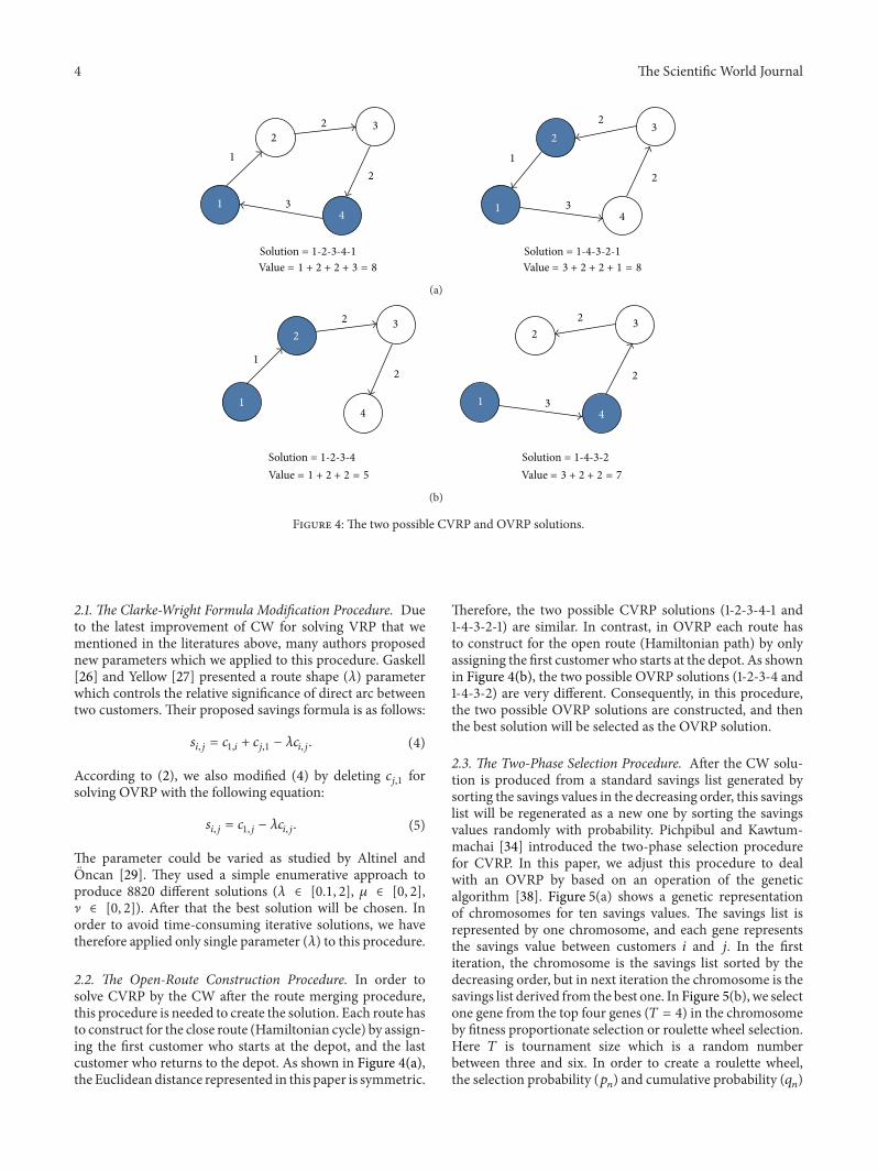
Figure 4: The two possible CVRP and OVRP solutions.

2.1. The Clarke-Wright Formula Modification Procedure. Dueto the latest improvement of CW for solving VRP that wementioned in the literatures above, many authors proposednew parameters which we applied to this procedure. Gaskell[26] and Yellow [27] presented a route shape (𝜆) parameterwhich controls the relative significance of direct arc betweentwo customers. Their proposed savings formula is as follows:

𝑠𝑖,𝑗 = 𝑐1,𝑖 + 𝑐𝑗,1 − 𝜆𝑐𝑖,𝑗. (4)

According to (2), we also modified (4) by deleting 𝑐𝑗,1 forsolving OVRP with the following equation:

𝑠𝑖,𝑗 = 𝑐1,𝑗 − 𝜆𝑐𝑖,𝑗. (5)

The parameter could be varied as studied by Altinel andOncan [29]. They used a simple enumerative approach toproduce 8820 different solutions (𝜆 ∈ [0.1, 2], 𝜇 ∈ [0, 2],] ∈ [0, 2]). After that the best solution will be chosen. Inorder to avoid time-consuming iterative solutions, we havetherefore applied only single parameter (𝜆) to this procedure.

2.2. The Open-Route Construction Procedure. In order tosolve CVRP by the CW after the route merging procedure,this procedure is needed to create the solution. Each route hasto construct for the close route (Hamiltonian cycle) by assign-ing the first customer who starts at the depot, and the lastcustomer who returns to the depot. As shown in Figure 4(a),the Euclidean distance represented in this paper is symmetric.

Therefore, the two possible CVRP solutions (1-2-3-4-1 and1-4-3-2-1) are similar. In contrast, in OVRP each route hasto construct for the open route (Hamiltonian path) by onlyassigning the first customer who starts at the depot. As shownin Figure 4(b), the two possible OVRP solutions (1-2-3-4 and1-4-3-2) are very different. Consequently, in this procedure,the two possible OVRP solutions are constructed, and thenthe best solution will be selected as the OVRP solution.

2.3. The Two-Phase Selection Procedure. After the CW solu-tion is produced from a standard savings list generated bysorting the savings values in the decreasing order, this savingslist will be regenerated as a new one by sorting the savingsvalues randomly with probability. Pichpibul and Kawtum-machai [34] introduced the two-phase selection procedurefor CVRP. In this paper, we adjust this procedure to dealwith an OVRP by based on an operation of the geneticalgorithm [38]. Figure 5(a) shows a genetic representationof chromosomes for ten savings values. The savings list isrepresented by one chromosome, and each gene representsthe savings value between customers 𝑖 and 𝑗. In the firstiteration, the chromosome is the savings list sorted by thedecreasing order, but in next iteration the chromosome is thesavings list derived from the best one. In Figure 5(b), we selectone gene from the top four genes (𝑇 = 4) in the chromosomeby fitness proportionate selection or roulette wheel selection.Here 𝑇 is tournament size which is a random numberbetween three and six. In order to create a roulette wheel,the selection probability (𝑝𝑛) and cumulative probability (𝑞𝑛)


1 2 3 4 5 6 7 8 9

1 2 3 4

1

1

1 2 3 4 5 6

2

1 2 3 4 5 6 7 8 9 10

(a)

(c)

(e)

Gene (n)

Savings (sn)

Savings (sn)

Savings (sn)

si,j

si,j

Savings (sn)

si,j

Savings (sn)

si,j

si,j

Savings (sn)

si,j

s2,6

s2,6

s2,6

s3,6 s3,5

s3,5

s3,5

s2,4

s2,4

s2,4

s2,5

s2,3

s2,3

s4,6

s4,6

s4,6

s5,6

s5,6

s3,6

s3,6

s5,6

s5,6

s4,5s2,6 s2,4 s3,5 s3,4s2,3

s2,5 s3,4 s4,5

s3,6

40.64

40.64

40.64

40.64 40.64

40.64

40.64 32.36 32.36

40.64

0.28 0.28 0.22 0.22

0.28

0.21 0.17

0.38

0.17

0.55 0.71 0.86

0.16 0.15 0.15

1.010.21

0.56 0.78 1.00

28.28

28.28

28.28 28.28 20.00 20.00 11.72

28.28

28.28

28.2830.58

30.58

30.58

32.3632.36

32.36 32.36

32.36 32.36

20.00 20.00

1 2 3 4 5 6 7 8 9 10Gene (n)

Savings (sn)

si,j s2,6 s2,3 s4,6 s5,6 s2,5 s3,4 s4,5s3,6 s2,4 s3,5

40.64 40.64 32.36 32.36 30.58 28.28 28.28 20.00 20.00 11.72

11.72

(b) T = 4

(d) T = 6

n

n

Pn

Pn

qn

qn

New gene (n)

New gene (n)

New gene (n)

Random spin (r) = 0.90

Random spin (r) = 0.38

Figure 5: The example of the two-phase selection procedure.

with savings value (𝑠𝑛) for each gene (𝑛) are calculated usingthe following equations:

𝑝𝑛 =𝑠𝑛

∑𝑖∈𝑇 𝑠𝑖

for 𝑛 ∈ 𝑇,

𝑞𝑛 = ∑

𝑖∈𝑛

𝑝𝑖 for 𝑛 ∈ 𝑇.(6)

After that, we spin the wheel with a random number (𝑟 =0.38) from the range between 0 and 1. The one savings value(𝑠2) will be selected to be a gene of a new chromosome byconsidering 𝑟 and 𝑞𝑛. If 𝑟 ≤ 𝑞1, then select the first savingsvalue 𝑠1; otherwise, select the 𝑛th savings value 𝑠𝑛 (2 ≤ 𝑛 ≤ 𝑇)

such that 𝑞𝑛−1 < 𝑟 ≤ 𝑞𝑛. The selected gene is removedfrom the chromosome which leaves nine savings values asshown in Figure 5(c). Figure 5(d) shows the same selectionprocess in the next iteration with parameters 𝑇 = 6 and𝑟 = 0.90. Therefore, this procedure will be executed until thelast gene of the chromosome is selected to be a gene of thenew chromosome which is shown in Figure 5(e).

When the new chromosome which represents the newsavings list is generated, it is calculated by the route mergingprocedure and the open-route construction procedure toproduce a new OVRP solution. After we compare twosolutions, the new chromosome will replace the previouschromosome only if the new solution is better than the


previous one. This acceptance criterion is referred to abasic variable neighborhood search which is to accept onlyimprovements [39]. Our approach is continued until thestopping criterion, which is the number of global iterationsfor two-phase selection, is satisfied.

2.4. The Route Postimprovement Procedure. In order to findany further improvements for the best solution found whenthe stopping criterion of the two-phase selection procedureis satisfied, we have developed the route postimprovementprocedure to generate different routes in our best solution.In order to explore the whole neighborhood of our bestsolution, we focus on the order of customers in single routecalled intraroute and multiple routes called interroute. Theneighborhood structures that we used are several well-knownmove operators found in the works of Subramanian et al. [35]andGroer et al. [36] including shiftmoves (1-0, 2-0, 3-0), swapmoves (1-1, 2-1, 2-2), and 𝜆-opt moves (𝜆 ∈ {2, 3}). The shiftmoves remove customers and insert them in another place.The swap moves select customers and exchange them. The𝜆-opt moves remove edges between customers and replacethem with new edges. Our scheme is adapted from the localsearch strategy found in Catay [40] by first applying a localneighborhood search to improve our best solution in eachroute. Then, a larger neighborhood search is applied acrosseach pair between routes, respectively, by using all eightmove operators with equal probability. This procedure isrepeated until the stopping criterion, which is the number ofconsecutive iterations without any improvements in the bestfound solution, is satisfied.

3. Computational Results

The proposed CW was coded in Visual Basic 6.0 on an IntelCore i7 CPU 860 clocked at 2.80GHz with 1.99GB of RAMunder Windows XP platform. The numerical experimentused five well-known data sets of Euclidean benchmarks(composed of 62 instances) of the OVRP consisting ofAugerat et al. [41] in data sets A, B, and P, Christofides andEilon [42] in data set E, and Fisher [43] in data set F.The inputdata is available online at http://www.branchandcut.org/ (lastaccess 1/2010). The best known solutions which are availableonline at http://www.hha.dk/∼lys/ (last access 7/2011) areobtained by a branch-and-cut algorithm from the work ofLetchford et al. [44]. In our approach, some parameters haveto be preset before the execution as shown in Table 1. Table 2describes the development of the proposed CW in detail.

The benchmark problem sizes that we highlighted in thispaper are classified as small-scale (less than 50 customers)and medium-scale (between 51 to 100 customers) with dif-ferent features, for example, uniformly and not uniformlydispersed customers, clustered and not clustered, with acentered or not centered depot. All problems also includecapacity constraints and minimum number of vehicles usedrestrictions. The first benchmark in data sets A, B, and Pwas proposed by Augerat et al. [41]. For the instances in dataset A, both customer locations and demands are randomlygenerated. The customer locations in data set B are clustered

Table 1: The parameters used in the proposed CW.

Parameter ValuesThe Clarke-Wright formula modificationprocedure

Route shape (𝜆) 0.1–2.0(increment of 0.1)

The two-phase selection procedure

Number of tournament sizes 3–20(random number)

Number of global iterations for two-phaseselection 5,000

The route postimprovement procedureNumber of consecutive iterations without anyimprovements in the best found solution 500

Probability to select each move operator 0.125

Table 2: The different features of the proposed CW.

Abbreviation Details

CW-1 Improve CW solution with Clarke-Wrightformula modification procedure

CW-2 Improve CW-1 solution with two-phase selectionprocedure

CW-3 Improve CW-2 solution with routepost-improvement procedure

instances. The modified version of other instances is data setP. In these data sets, the problem ranges in size from 16 to69 customers including the depot. The second benchmarkin data set E was proposed by Christofides and Eilon [42].In this data set, the customers are randomly distributed inthe plane and the depot is either in the center or near toit. The problem ranges in size from 22 to 101 customersincluding the depot. The third benchmark in data set F isthe real-life problem given by Fisher [43]. Instances F-n45-k4and F-n135-k7 represent a day of grocery deliveries from thePeterboro and Bramalea, Ontario terminals, respectively, ofNational Grocers Limited. Instance F-n72-k4 represents thedelivery of tires, batteries, and accessories to gasoline servicestations. The depot is not centered in both instances. Theproblem ranges in size from 45 to 135 customers includingthe depot. We discuss each benchmark problem in whichthe percentage improvement between CW solution (cws) andobtained solution (obs) is calculated as follows:

Percentage improvement = (cws − obscws) × 100. (7)

Moreover, the percentage deviation between obtained solu-tion (obs) and the best known solution (bks) is also calculatedas follows:

Percentage deviation = (obs − bksbks) × 100. (8)

The computational results for OVRP benchmark instances ofAugerat et al. [41], Christofides and Eilon [42], and Fisher[43] are reported in Tables 3–5. We do not only consider the


Table 3: Computational results between the proposed CW and CW for data sets A, B, P, E, C, and F.

Number Instance Solution Percentage improvement CPU time (seconds)CW CW-1 𝜆 CW-2 CW-3 CW-1 CW-2 CW-3

1 A-n32-k5 612.99 535.92 1.7 493.18 487.31 12.571 19.544 20.503 4.8192 A-n33-k5 496.61 458.52 1.5 425.54 424.54 7.669 14.311 14.512 5.4933 A-n33-k6 566.16 546.18 1.7 464.10 462.43 3.528 18.026 18.321 5.2894 A-n34-k5 547.27 520.09 1.1 519.51 508.17 4.966 5.071 7.143 5.6755 A-n36-k5 689.48 571.70 1.8 535.23 519.46 17.083 22.373 24.660 6.1346 A-n37-k5 579.74 541.64 1.9 511.12 486.24 6.572 11.836 16.128 6.6897 A-n37-k6 712.86 612.76 1.9 616.26 581.07 14.041 13.551 18.487 6.8258 A-n38-k5 552.83 520.78 1.6 531.49 498.00 5.796 3.859 9.918 7.0929 A-n39-k5 704.55 590.71 1.2 554.80 549.68 16.158 21.254 21.980 7.56810 A-n39-k6 720.55 558.86 1.9 547.57 533.07 22.439 24.007 26.019 7.49411 A-n44-k6 757.90 724.33 1.1 641.77 617.39 4.430 15.323 18.540 10.32312 A-n45-k6 734.97 643.56 2.0 716.52 648.67 12.437 2.511 11.742 10.41413 A-n45-k7 829.44 759.40 1.6 699.86 685.16 8.444 15.622 17.395 10.75414 A-n46-k7 738.00 645.24 1.1 593.57 583.54 12.569 19.570 20.930 11.25915 A-n48-k7 789.39 756.58 1.1 726.54 669.83 4.156 7.962 15.146 12.53416 A-n53-k7 816.38 702.85 1.5 665.39 655.18 13.907 18.495 19.746 15.62417 A-n54-k7 951.51 808.42 1.5 723.60 709.27 15.038 23.952 25.458 16.22418 A-n55-k9 802.06 736.91 1.9 696.52 669.06 8.123 13.158 16.582 17.32419 A-n62-k8 979.51 851.15 1.3 815.21 783.18 13.105 16.774 20.044 22.95920 A-n65-k9 844.35 800.41 1.2 783.42 728.59 5.205 7.217 13.710 24.52421 A-n69-k9 942.87 798.64 2.0 773.17 757.76 15.296 17.998 19.632 28.600

Average percentage improvement of data set A 10.644 14.877 17.933 11.6011 B-n31-k5 383.68 367.00 0.9 364.80 362.73 4.347 4.923 5.463 4.3652 B-n34-k5 541.34 506.26 0.9 459.59 458.76 6.480 15.103 15.254 5.5563 B-n35-k5 599.16 595.15 1.4 567.34 557.33 0.669 5.311 6.982 5.9814 B-n38-k6 500.64 483.14 1.4 450.72 445.63 3.495 9.972 10.989 7.1095 B-n39-k5 382.11 354.03 1.4 334.70 322.54 7.350 12.409 15.590 7.6026 B-n41-k6 539.15 507.25 1.8 493.34 483.07 5.917 8.496 10.402 8.5497 B-n43-k6 483.21 481.57 1.6 432.30 428.17 0.340 10.536 11.391 9.4228 B-n44-k7 575.52 560.54 1.9 512.64 501.31 2.603 10.927 12.895 10.2449 B-n45-k5 601.71 512.73 1.9 509.56 488.07 14.788 15.315 18.887 10.35710 B-n45-k6 459.90 430.83 1.1 431.54 403.81 6.323 6.168 12.197 10.57311 B-n50-k7 537.23 491.93 1.9 446.07 437.15 8.433 16.969 18.629 13.26512 B-n51-k7 703.81 683.31 2.0 656.01 625.14 2.913 6.792 11.178 13.50913 B-n52-k7 482.90 465.17 1.8 450.07 441.19 3.672 6.798 8.637 14.58614 B-n56-k7 497.15 474.13 1.5 463.06 420.48 4.629 6.856 15.420 17.40915 B-n63-k10 950.48 950.48 1.0 857.90 837.07 0.000 9.740 11.931 23.72416 B-n64-k9 572.41 541.70 1.2 581.72 520.47 5.364 −1.627 9.074 23.76417 B-n68-k9 830.48 777.68 1.1 758.69 701.72 6.357 8.644 15.504 27.874

Average percentage improvement of data set B 4.922 9.020 12.378 12.5821 P-n16-k8 235.89 235.89 0.3 235.06 235.06 0.000 0.352 0.352 1.1732 P-n19-k2 198.25 172.93 1.9 168.57 168.57 12.771 14.972 14.972 1.5653 P-n20-k2 210.01 184.50 1.9 170.28 170.28 12.147 18.918 18.918 1.7124 P-n21-k2 209.92 180.27 1.8 168.15 163.88 14.124 19.897 21.933 1.729


Table 3: Continued.

Number Instance Solution Percentage improvement CPU time (seconds)CW CW-1 𝜆 CW-2 CW-3 CW-1 CW-2 CW-3

5 P-n22-k2 206.00 183.58 1.8 171.46 167.19 10.883 16.765 18.840 1.8886 P-n22-k8 370.26 345.53 1.6 352.14 345.87 6.679 4.892 6.588 2.3307 P-n23-k8 309.74 307.28 1.7 304.83 302.87 0.794 1.586 2.219 2.6088 P-n40-k5 420.65 395.73 1.5 370.64 349.55 5.924 11.889 16.902 7.7499 P-n45-k5 459.29 442.23 1.5 396.64 391.81 3.714 13.641 14.692 10.15910 P-n50-k7 468.42 447.69 1.5 440.56 397.38 4.426 5.948 15.167 13.23711 P-n55-k7 513.45 464.90 1.4 452.69 411.58 9.455 11.833 19.840 16.62712 P-n55-k8 505.72 476.43 1.8 442.21 412.55 5.793 12.558 18.423 16.34913 P-n55-k10 555.25 502.56 1.6 488.65 444.31 9.490 11.995 19.981 17.38714 P-n60-k10 584.40 539.43 1.8 503.38 482.09 7.694 13.864 17.507 20.49915 P-n65-k10 649.31 592.35 1.6 531.57 522.50 8.772 18.133 19.529 29.626

Average percentage improvement of data set P 7.511 11.816 15.058 9.6421 E-n22-k4 286.91 260.61 1.3 252.61 252.61 9.169 11.955 11.955 3.7532 E-n23-k3 497.18 456.86 1.2 444.29 442.98 8.111 10.638 10.901 4.1563 E-n33-k4 633.04 576.29 1.4 518.04 511.26 8.965 18.165 19.236 12.2234 E-n51-k5 493.02 477.78 2.0 452.67 416.06 3.091 8.185 15.610 36.1545 E-n76-k10 697.03 641.48 1.9 587.35 567.14 7.971 15.736 18.635 68.9176 E-n101-k8 807.33 724.48 2.0 694.88 642.36 10.262 13.929 20.433 82.387

Average percentage improvement of data set E 7.928 13.101 16.128 34.5981 F-n45-k4 615.12 535.85 2.0 478.40 463.90 12.886 22.227 24.584 10.3652 F-n72-k4 208.29 191.18 2.0 187.67 177.00 8.212 9.899 15.021 42.5543 F-n135-k7 1033.24 856.33 1.9 816.30 775.80 17.122 20.996 24.916 112.258

Average percentage improvement of data set F 12.740 17.707 21.507 55.059Italic number indicates the infeasible solution (the number of vehicles used is inadequate).

Table 4: Computational results between the proposed CW and MA for data sets A, P, and F.

Number Instance Solution Percentage deviationBest Known MA Our CW MA Our CW

1 A-n32-k5 487.31 487.31 487.31 0.000 0.0002 A-n33-k5 424.54 424.54 424.54 0.000 0.0003 A-n33-k6 462.43 462.43 462.43 0.000 0.0004 A-n34-k5 508.17 508.52 508.17 0.068 0.0005 A-n36-k5 519.46 519.46 519.46 0.000 0.0006 A-n37-k5 486.24 486.24 486.24 0.000 0.0007 P-n19-k2 168.57 168.57 168.57 0.000 0.0008 P-n20-k2 170.28 170.28 170.28 0.000 0.0009 P-n21-k2 163.88 163.88 163.88 0.000 0.00010 P-n22-k2 167.19 167.19 167.19 0.000 0.00011 P-n40-k5 349.55 349.55 349.55 0.000 0.00012 P-n45-k5 391.81 391.81 391.81 0.000 0.00013 P-n50-k7 397.38 407.73 397.38 2.605 0.00014 F-n45-k4 463.90 463.90 463.90 0.000 0.00015 F-n72-k4 177.00 177.45 177.00 0.257 0.000

Average percentage deviation of data sets A, P, and F 0.195 0.000


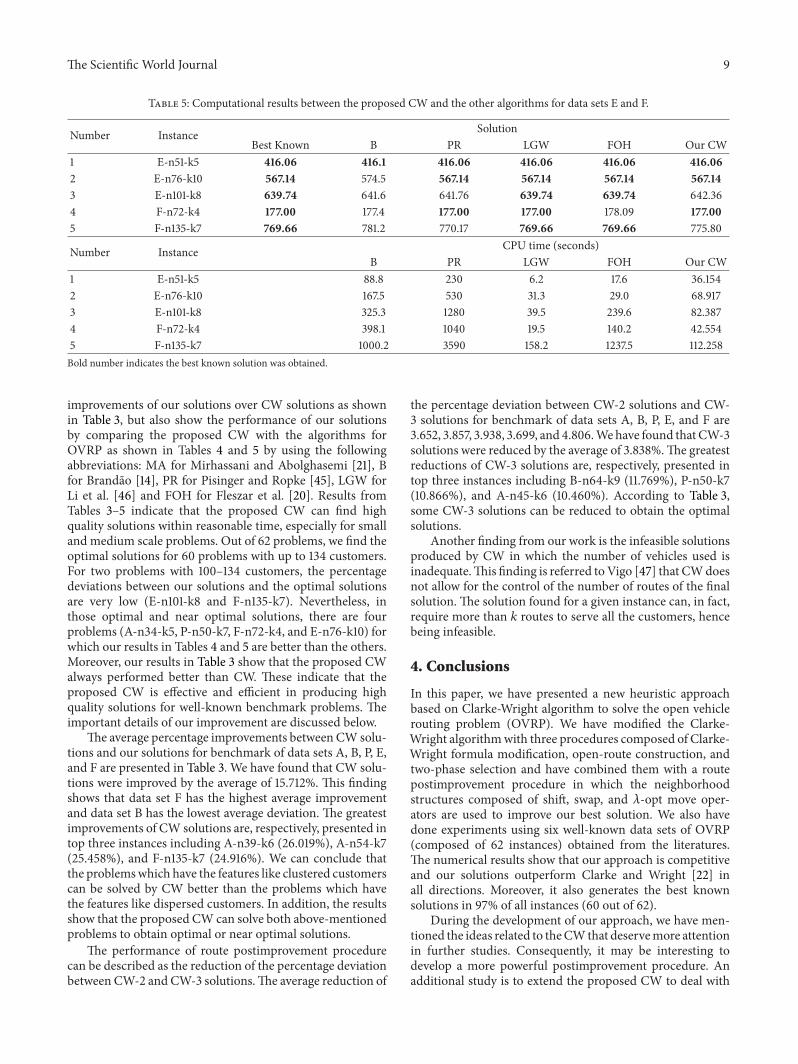
Table 5: Computational results between the proposed CW and the other algorithms for data sets E and F.

Number Instance SolutionBest Known B PR LGW FOH Our CW

1 E-n51-k5 416.06 416.1 416.06 416.06 416.06 416.062 E-n76-k10 567.14 574.5 567.14 567.14 567.14 567.143 E-n101-k8 639.74 641.6 641.76 639.74 639.74 642.364 F-n72-k4 177.00 177.4 177.00 177.00 178.09 177.005 F-n135-k7 769.66 781.2 770.17 769.66 769.66 775.80

Number Instance CPU time (seconds)B PR LGW FOH Our CW

1 E-n51-k5 88.8 230 6.2 17.6 36.1542 E-n76-k10 167.5 530 31.3 29.0 68.9173 E-n101-k8 325.3 1280 39.5 239.6 82.3874 F-n72-k4 398.1 1040 19.5 140.2 42.5545 F-n135-k7 1000.2 3590 158.2 1237.5 112.258Bold number indicates the best known solution was obtained.

improvements of our solutions over CW solutions as shownin Table 3, but also show the performance of our solutionsby comparing the proposed CW with the algorithms forOVRP as shown in Tables 4 and 5 by using the followingabbreviations: MA for Mirhassani and Abolghasemi [21], Bfor Brandao [14], PR for Pisinger and Ropke [45], LGW forLi et al. [46] and FOH for Fleszar et al. [20]. Results fromTables 3–5 indicate that the proposed CW can find highquality solutions within reasonable time, especially for smalland medium scale problems. Out of 62 problems, we find theoptimal solutions for 60 problems with up to 134 customers.For two problems with 100–134 customers, the percentagedeviations between our solutions and the optimal solutionsare very low (E-n101-k8 and F-n135-k7). Nevertheless, inthose optimal and near optimal solutions, there are fourproblems (A-n34-k5, P-n50-k7, F-n72-k4, and E-n76-k10) forwhich our results in Tables 4 and 5 are better than the others.Moreover, our results in Table 3 show that the proposed CWalways performed better than CW. These indicate that theproposed CW is effective and efficient in producing highquality solutions for well-known benchmark problems. Theimportant details of our improvement are discussed below.

The average percentage improvements between CW solu-tions and our solutions for benchmark of data sets A, B, P, E,and F are presented in Table 3. We have found that CW solu-tions were improved by the average of 15.712%. This findingshows that data set F has the highest average improvementand data set B has the lowest average deviation. The greatestimprovements of CW solutions are, respectively, presented intop three instances including A-n39-k6 (26.019%), A-n54-k7(25.458%), and F-n135-k7 (24.916%). We can conclude thatthe problemswhich have the features like clustered customerscan be solved by CW better than the problems which havethe features like dispersed customers. In addition, the resultsshow that the proposed CW can solve both above-mentionedproblems to obtain optimal or near optimal solutions.

The performance of route postimprovement procedurecan be described as the reduction of the percentage deviationbetween CW-2 and CW-3 solutions.The average reduction of

the percentage deviation between CW-2 solutions and CW-3 solutions for benchmark of data sets A, B, P, E, and F are3.652, 3.857, 3.938, 3.699, and 4.806.Wehave found that CW-3solutions were reduced by the average of 3.838%.The greatestreductions of CW-3 solutions are, respectively, presented intop three instances including B-n64-k9 (11.769%), P-n50-k7(10.866%), and A-n45-k6 (10.460%). According to Table 3,some CW-3 solutions can be reduced to obtain the optimalsolutions.

Another finding from our work is the infeasible solutionsproduced by CW in which the number of vehicles used isinadequate.This finding is referred toVigo [47] that CWdoesnot allow for the control of the number of routes of the finalsolution. The solution found for a given instance can, in fact,require more than 𝑘 routes to serve all the customers, hencebeing infeasible.

4. Conclusions

In this paper, we have presented a new heuristic approachbased on Clarke-Wright algorithm to solve the open vehiclerouting problem (OVRP). We have modified the Clarke-Wright algorithmwith three procedures composed of Clarke-Wright formula modification, open-route construction, andtwo-phase selection and have combined them with a routepostimprovement procedure in which the neighborhoodstructures composed of shift, swap, and 𝜆-opt move oper-ators are used to improve our best solution. We also havedone experiments using six well-known data sets of OVRP(composed of 62 instances) obtained from the literatures.The numerical results show that our approach is competitiveand our solutions outperform Clarke and Wright [22] inall directions. Moreover, it also generates the best knownsolutions in 97% of all instances (60 out of 62).

During the development of our approach, we have men-tioned the ideas related to theCWthat deservemore attentionin further studies. Consequently, it may be interesting todevelop a more powerful postimprovement procedure. Anadditional study is to extend the proposed CW to deal with


other variants of the studied problems such as simultaneouspickup and delivery (VRPSPD) or time windows (VRPTW).

References

[1] D. Sariklis and S. Powell, “A heuristic method for the open vehi-cle routing problem,” The Journal of the Operational ResearchSociety, vol. 51, no. 5, pp. 564–573, 2000.

[2] Z. Fu and M. Wright, “Train plan model for British railfreight services through the channel tunnel,”The Journal of theOperational Research Society, vol. 45, no. 4, pp. 384–391, 1994.

[3] L. Y. O. Li and Z. Fu, “The school bus routing problem: a casestudy,” The Journal of the Operational Research Society, vol. 53,no. 5, pp. 552–558, 2002.

[4] C. D. Tarantilis and C. T. Kiranoudis, “Distribution of freshmeat,” Journal of Food Engineering, vol. 51, no. 1, pp. 85–91, 2002.

[5] R. Russell, W.-C. Chiang, and D. Zepeda, “Integrating multi-product production and distribution in newspaper logistics,”Computers & Operations Research, vol. 35, no. 5, pp. 1576–1588,2008.

[6] W.-C. Chiang, R. Russell, X. Xu, and D. Zepeda, “A simu-lation/metaheuristic approach to newspaper production anddistribution supply chain problems,” International Journal ofProduction Economics, vol. 121, no. 2, pp. 752–767, 2009.

[7] P. P. Repoussis, D. C. Paraskevopoulos, G. Zobolas, C. D.Tarantilis, and G. Ioannou, “A web-based decision supportsystem for waste lube oils collection and recycling,” EuropeanJournal of Operational Research, vol. 195, no. 3, pp. 676–700,2009.

[8] S. Yu, C. Ding, andK. Zhu, “A hybrid GA-TS algorithm for openvehicle routing optimization of coal mines material,” ExpertSystems with Applications, vol. 38, no. 8, pp. 10568–10573, 2011.

[9] N. Christofides, “Worst-case analysis of a new heuristic for thetravelling salesman problem,” Tech. Rep. 388, Graduate Schoolof Industrial Administration, Canegie Mellon University, 1976.

[10] M. Held and R. M. Karp, “The traveling salesman problemand minimum spanning trees,” Operations Research, vol. 18, pp.1138–1162, 1970.

[11] R. E. Miller and J. W. Thatcher, Complexity of ComputerComputations, Plenum Press, New York, NY, USA, 1972.

[12] M. Syslo, N. Deo, and J. Kowaklik, Discrete OptimizationAlgorithms with Pascal Programs, Prentice Hall, EnglewoodCliffs, NJ, USA, 1983.

[13] P. Toth and D. Vigo, The Vehicle Routing Problem, SIAMMonographs on Discrete Mathematics and Applications, SIAMPublishing, Philadelphia, Pa, USA, 2002.

[14] J. Brandao, “A tabu search algorithm for the open vehicle routingproblem,” European Journal of Operational Research, vol. 157, no.3, pp. 552–564, 2004.

[15] M. Salari, P. Toth, and A. Tramontani, “An ILP improvementprocedure for the Open Vehicle Routing Problem,” Computers& Operations Research, vol. 37, no. 12, pp. 2106–2120, 2010.

[16] G. B. Dantzig and J. H. Ramser, “The truck dispatchingproblem,”Management Science, vol. 6, pp. 80–91, 1959.

[17] C. D. Tarantilis, D. Diakoulaki, and C. T. Kiranoudis, “Combi-nation of geographical information system and efficient routingalgorithms for real life distribution operations,” European Jour-nal of Operational Research, vol. 152, no. 2, pp. 437–453, 2004.

[18] Z. Fu, R. Eglese, and L. Li, “A new tabu search heuristic for theopen vehicle routing problem,” The Journal of the OperationalResearch Society, vol. 56, no. 3, pp. 267–274, 2005.

[19] X. Li and P. Tian, “An ant colony system for the open vehiclerouting problem,” in Ant Colony Optimization and SwarmIntelligence, M. Dorigo, L. M. Gambardella, M. Birattari, A.Martinoli, R. Poli, and T. Stutzle, Eds., vol. 4150 of Lecture Notesin Computer Science, pp. 356–363, Springer, Berlin, Germany,2006.

[20] K. Fleszar, I. H. Osman, and K. S. Hindi, “A variable neighbour-hood search algorithm for the open vehicle routing problem,”European Journal of Operational Research, vol. 195, no. 3, pp.803–809, 2009.

[21] S. A. Mirhassani and N. Abolghasemi, “A particle swarmoptimization algorithm for open vehicle routing problem,”Expert Systems with Applications, vol. 38, no. 9, pp. 11547–11551,2011.

[22] G. Clarke and J. W. Wright, “Scheduling of vehicles froma central depot to a number of delivery points,” OperationsResearch, vol. 12, pp. 568–581, 1964.

[23] F. A. Tillman, “The multiple terminal delivery problem withprobabilistic demands,” Transportation Science, vol. 3, pp. 192–204, 1969.

[24] L. Bodin, B. Golden, A. Assad, and M. Ball, “Routing andscheduling of vehicles and crews. The state of the art,” Comput-ers & Operations Research, vol. 10, no. 2, pp. 63–211, 1983.

[25] I. Deif and L. D. Bodin, “Extension of the Clarke-Wrightalgorithm for solving the vehicle routing problem with back-hauling,” in Proceedings of the Babson Conference on SoftwareUses in Transportation and Logistics Management, A. E. Kidder,Ed., pp. 75–96, Babson Park, Mass, USA, 1984.

[26] T. J. Gaskell, “Bases for vehicle fleet scheduling,” OperationalResearch Quarterly, vol. 18, pp. 281–295, 1967.

[27] P. Yellow, “A computational modification to the savings methodof vehicle scheduling,” Operational Research Quarterly, vol. 21,pp. 281–283, 1970.

[28] H. Paessens, “The savings algorithm for the vehicle routingproblem,” European Journal of Operational Research, vol. 34, no.3, pp. 336–344, 1988.

[29] I. K. Altinel and T. Oncan, “A new enhancement of the ClarkeandWright savings heuristic for the capacitated vehicle routingproblem,” The Journal of the Operational Research Society, vol.56, no. 8, pp. 954–961, 2005.

[30] T. Doyuran and B. Catay, “A robust enhancement to the Clarke-Wright savings algorithm,” The Journal of the OperationalResearch Society, vol. 62, no. 1, pp. 223–231, 2011.

[31] A. A. Juan, J. Faulin, R. Ruiz, B. Barrios, and S. Caballe, “TheSR-GCWS hybrid algorithm for solving the capacitated vehiclerouting problem,” Applied Soft Computing Journal, vol. 10, no. 1,pp. 215–224, 2010.

[32] A. A. Juan, J. Faulin, J. Jorba, D. Riera, D. Masip, and B.Barrios, “On the use of Monte Carlo simulation, cache andsplitting techniques to improve the Clarke and Wright savingsheuristics,”The Journal of the Operational Research Society, vol.62, no. 6, pp. 1085–1097, 2011.

[33] T. Pichpibul and R. Kawtummachai, “New enhancementfor Clarke-Wright savings algorithm to optimize the capaci-tated vehicle routing problem,” European Journal of ScientificResearch, vol. 78, pp. 119–134, 2012.

[34] T. Pichpibul and R. Kawtummachai, “An improved Clarke andWright savings algorithm for the capacitated vehicle routingproblem,” ScienceAsia, vol. 38, pp. 307–318, 2012.

[35] A. Subramanian, L. M. A. Drummond, C. Bentes, L. S. Ochi,and R. Farias, “A parallel heuristic for the vehicle routing


problem with simultaneous pickup and delivery,” Computers &Operations Research, vol. 37, no. 11, pp. 1899–1911, 2010.

[36] C. Groer, B. Golden, and E. Wasil, “A library of local searchheuristics for the vehicle routing problem,” Mathematical Pro-gramming Computation, vol. 2, no. 2, pp. 79–101, 2010.

[37] G. Laporte, M. Gendreau, J. Potvin, and F. Semet, “Classicaland modern heuristics for the vehicle routing problem,” Inter-national Transactions in Operational Research, vol. 7, no. 4-5, pp.285–300, 2000.

[38] M. Gen and R. Cheng, Genetic Algorithms and EngineeringDesign, John Wiley & Sons, New York, NY, USA, 1997.

[39] V. C. Hemmelmayr, K. F. Doerner, and R. F. Hartl, “A variableneighborhood search heuristic for periodic routing problems,”European Journal of Operational Research, vol. 195, no. 3, pp.791–802, 2009.

[40] B. Catay, “A new saving-based ant algorithm for the vehiclerouting problemwith simultaneous pickup anddelivery,”ExpertSystems with Applications, vol. 37, no. 10, pp. 6809–6817, 2010.

[41] P. Augerat, J. Belenguer, E. Benavent, A. Corbern, D. Naddef,and G. Rinaldi, “Computational results with a branch and cutcode for the capacitated vehicle routing problem,” ResearchReport 949-M, Universite Joseph Fourier, Grenoble, France,1995.

[42] N. Christofides and S. Eilon, “An algorithm for the vehicledispatching problem,” Operational Research Quarterly, vol. 20,pp. 309–318, 1969.

[43] M. L. Fisher, “Optimal solution of vehicle routing problemsusingminimumK-trees,”Operations Research, vol. 42, no. 4, pp.626–642, 1994.

[44] A. N. Letchford, J. Lysgaard, and R. W. Eglese, “A branch-and-cut algorithm for the capacitated open vehicle routing problem,”The Journal of the Operational Research Society, vol. 58, no. 12,pp. 1642–1651, 2007.

[45] D. Pisinger and S. Ropke, “A general heuristic for vehicle routingproblems,” Computers & Operations Research, vol. 34, no. 8, pp.2403–2435, 2007.

[46] F. Li, B. Golden, and E. Wasil, “The open vehicle routing prob-lem: algorithms, large-scale test problems, and computationalresults,” Computers & Operations Research, vol. 34, no. 10, pp.2918–2930, 2007.

[47] D. Vigo, “Heuristic algorithm for the asymmetric capacitatedvehicle routing problem,” European Journal of OperationalResearch, vol. 89, no. 1, pp. 108–126, 1996.

Submit your manuscripts athttp://www.hindawi.com

Computer Games Technology

International Journal of

Hindawi Publishing Corporationhttp://www.hindawi.com Volume 2014


Distributed Sensor Networks


Advances in

FuzzySystems

Hindawi Publishing Corporationhttp://www.hindawi.com

Volume 2014


ReconfigurableComputing

Hindawi Publishing Corporation http://www.hindawi.com Volume 2014


Applied Computational Intelligence and Soft Computing

Advances in

Artificial Intelligence


Advances inSoftware EngineeringHindawi Publishing Corporationhttp://www.hindawi.com Volume 2014


Electrical and Computer Engineering

Journal of

Journal of

Computer Networks and Communications


Hindawi Publishing Corporation

http://www.hindawi.com Volume 2014

Advances in

Multimedia


Biomedical Imaging


ArtificialNeural Systems

Advances in


RoboticsJournal of



Computational Intelligence and Neuroscience

Industrial EngineeringJournal of


Modelling & Simulation in EngineeringHindawi Publishing Corporation http://www.hindawi.com Volume 2014

The Scientific World JournalHindawi Publishing Corporation http://www.hindawi.com Volume 2014


Human-ComputerInteraction

Advances in

Computer EngineeringAdvances in


research article a heuristic approach based on clarke...

Documents