reprint indian journal of economics and development
TRANSCRIPT

Print ISSN 2277-5412 Online ISSN 2322-0430
Volume 12 No. 2April-June, 2016
Indian Journal of Economics and Development
Society of Economics and Developmentwww.soed.in
2004
Reprint

Indian Journal of Economics and DevelopmentEditorial Board
Chief Editor
Dr. S.S. ChahalFormer Director, Techonology Marketing and IPR Cell, Punjab Agricultural University, Ludhiana(India)
EditorsDr. S.S. Chhina, Former Dean, Faculty of Agriculture, Khalsa College, AmritsarDr. P. Kataria, Punjab Agricultural University, Ludhiana (India)Dr. Shalini Sharma, Punjab Agricultural University, Ludhiana (India)Dr. Sanjay Kumar, Punjab Agricultural University, Ludhiana (India)
MembersDr. Inderpal Singh, Trade and Investment, Economic Policy and Strategy, NSW (Australia)Dr. Timothy J. Colwill, Research Economist, Agriculture and Agri-food Canada, Ottawa (Canada)
Dr. Ravinderpal Singh Gill, Agriculture and Agri-Food Canada, Ottawa (Canada)Dr. Richard Kwasi Bannor, Ministry of Food and Agriculture, Kasoa-GhanaDr. I.P. Singh, SK Rajasthan Agricultural University, Bikaner (India)
Dr. J.L. Sharma, Eternal University, Baru Sahib (India)
Dr. K.K. Datta, National Dairy Research Institute, Karnal (India)
Dr. A.K. Vasisht, Indian Agricultural Statistics Research Institute, New Delhi (India)
Dr. V.P. Luhach, CCS Haryana Agricultural University, Hisar (India)
Dr. M.K.Sekhon, Punjab Agricultural University, Ludhiana (India)
Dr. Y.C. Singh, Central Agricultural University, Manipur (India)Dr. Jasdev Singh, Punjab Agricultural University, Ludhiana (India)Dr. Seema Bathla, Jawaharlal Nehru University, New Delhi (India)
Dr. R.B.Hile, MPKV, Rahuri (India)Dr. Baljinder Kaur Sidana, Punjab Agricultural University, Ludhiana (India)
Dr. Naresh Singla, Central University of Punjab, Bathinda
Dr. Sadiq Mohammed Sanusi, Federal University of Technology, Minna (Nigeria)
Dr. Rohit Singla, Boston College, Fulton (USA)
Dr. Deepak Upadhya, Local Initiatives for Biodiversity, Research and Development, Pokhara, Kaski (Nepal)
Ms. Donata Ponsian Kemirembe, Division of Environment, Vice President’s Office, Dar es Salaam (Tanzania)

Print ISSN 2277-5412Online ISSN 2322-0430
Indian Journal of Economics and Development
Society of Economics and Developmentwww.soed.in
Indian Journal of Economics and DevelopmentVolume 12 (2) 2016
©Society of Economics and Development
Printed and Published by Dr. Parminder Kaur on the behalf of the Society of Economics andDevelopment
Email: [email protected]: www.soed.inJournal is available on www.indianjournals.com
Printed at PRINTVIZION1766/1, Street No. 2Maharaj NagarLudhiana-141004Phone: 0161-4612199Email: [email protected]

Indian Journal of Economics and Development(Journal of the Society of Economics and Development)
Volume 12 April-June, 2016 No. 2Contents
Review ArticleChallenges and prospects of convenience food in India: An overview 203
Shivani Verma and Ramandeep Singh
Research ArticlesDomestic water consumption pattern and its linkage with socio-economic variables: A case study ofLudhiana city
215
Jasdeep Kaur, A.S. Bhullar, and R.S. GhumanSweet potato in Nigeria: Trends and socio-economic characteristics of farmers in selected local governmentarea of Kano state
223
Isah Musa Ahmad, Makama S.A., and Babagana G.A.Socio-economic impact of enterprises adoption on self-help group households in Punjab 229
Nirbhai Singh, Sanjay Kumar, and Jasdev SinghRelationship between urbanisation and economic growth: A causality analysis for India 237
Laxmi NarayanCost and return structure of tomato growers under open field, low tunnel and poly house conditions 243
Gurhemdeep Singh, J.S.Sidhu, and Jasdev SinghComposition, intensity and competitiveness of agricultural trade between India and ASEAN 249
Renjini V.R. and Amit KarStructure of assets among households in rural Punjab: An empirical analysis 255
Sukhdev Singh, Jasdeep Singh Toor, and Balwinder SinghAgricultural resource and income inequality in Northern Rajasthan 265
Mada Melkamu and N.K SinghBSE SME equity financing platform: A study of index risk return paradoxn 273
Amanjot Singh and Parneet KaurLevel of income, expenditure behaviour and poverty among farming community in rural Bihar 283
Ghanshyam PandayEconomic evaluation of Badrigad Watershed, Uttarakhand 293
Subhash Chandra and K.P. RaverkarSocio-economics of herbal processing units in Himachal Pradesh 301
Sukhjinder Singh and Sharanjit Singh DhillonAnalysis of growth, distributional pattern and density of tractors in India with special reference to Punjab 307
Vanusha Baregal and D.K.GroverInvestigating the relationship between transport infrastructure and economic growth: The case of India 315
Geet Kalra, Varun Chotia and Amit GoelSocio-economic factors affecting adoption behaviour of farmers for net-house vegetable cultivation inPunjab
321
Manjeet Kaur, M.K. Sekhon, Amrit Kaur Mahal, and Rakhi AroraAn empirical analysis of pilgrimage tourism in Jammu and Kashmir 327
Ruhi Refath Aara and Paramjeet Kaur Dhindhsa

Economic analysis of milk production among small holder dairy farmers in Punjab: A case study of Amritsardistrict
335
Kashish, Manjeet Kaur, M.K. Sekhon, and Vikrant DhawanHuman trafficking: A case of deceived aspiring emigrants in Punjab 341
Shivani Sharma, Simran Kang Sidhu, and Shalini SharmaResearch NotesProfit efficiency among smallholders milk producers in Mizoram state 347
Lalrinsangpuii, R. Malhotra, and Laishram PriscillaEconomic analysis of milk production and marketed surplus in Chittorgarh district of Rajasthan 353
R.L. Bairwa, A.K. Chauhan, and Bulbul G.. NagraleEconomics and growth performance of chrysanthemumf flower in Tumkur district of Karnataka 359
Gunabhagya, S.S. Guledgudda, and B.C. RajurCotton cultivation in Punjab: An economic analysis 365
Shaminder Kumar and J. SachdevaEntrepreneurial behaviour of vegetable growers in Karnataka 369
N. Kumara, A. Nehal Farooquee, and P.V.K.SasidharDeterminants of participation of dairy farmers in dairy cooperative societies in Manipur 377
L. Priscilla, A.K. Chauhan, Lalrinsangpuii, and Bulbul G. NagraleProviding social security through public expenditure: An evidendce from India’s largest employment guaranteeprogramme
381
Paramita Saha and Soma DebnathEvaluation of vocational training programmes on mushroom cultivation 393
Dharminder Singh and K.B. SinghEconomics of farm business of selected small farmers in Akola district of Maharashtra 399
Aditi S. Ghevade, G.D.Rede, and G. B. Malthane
Abstracts (Ph.D./M.Phil./M.Sc. Theses) 405

.
INDEXING AND ABSTRACTING SOURCESIndian Journal of Economics and Development
Indexing and Abstracting Sources WebsiteAcademicKeys www.socialsciences.academickeys.comAdvanced Science Index www,journal-index.orgAcademic Resource Index (Research Bible) www.journalseeker.researchbib.comAmerican Economic Association (JEL) www.aeaweb.org
Centre for Agriculture and Biosciences www.cabi.orgInternational (CABI)Cite Factor www.citefactor.orgCrossref www.crossref.orgCNKI Scholar www.eng.scholar.cnki.netDirectory of Research Journals Indexing www.drji.orgDirectory of Science www.directorofscience.comDiva Enterprises Private Limited www.indianjournals.comEurasian Scientific Journal Index www.esjindex.orgGlobal Impact Factor (2015: 0.435) www.globalimpactfactor.com
Google Scholar www.scholar.google.co.inIndian Science and Research www.indianscience.inInfobase Index www.infobaseindex.comInstitute for Information Resources www.rjifactor.comInternational Impact Factor Services www.impactfactorservice.comInternational Society for Research Activity www.israjif.orgJIFACTOR www.jifactor.orgJ-Gate www.jgateplus.comNational Academy of Agricultural Sciences www.naasindia.orgNational Documentation Centre www.eskep.ekt.grScientific Indexing Services www.sindexs.org
Ulrichsweb Global Serials Directory www.ulrichsweb.serialssolutions.comWorldCat www.worldcat.orgYahoo Search www.in.search.yahoo.com

Society of Economics and DevelopmentObjectives
1. To promote awareness on the issues relating to economic development.2. To promote better social and ethical values to promote development.3. To promote economic prosperity and serve as a tool to create the consciousness for development.4. To conduct research and publish reports on economic issues.5. To organize seminars, symposia, workshops to discuss the economic problems.6. To offer consultancy, liaison and services as a facilitator.
Executive CommitteeFounder President
Dr. S.S. Chhina, Former Dean, Faculty of Agriculture, Khasla College, Amritsar
PresidentDr. M.S. Toor, Professor of Economics, PAU, Ludhiana
Vice PresidentsDr. D.K. Grover, Director, AERC, PAU, LudhianaDr. A.K. Chauhan, Principal Scientist (Dairy Economics), NDRI, KarnalDr. Simran K. Sidhu, Professor of Sociology, PAU, LudhianaDr. Pratibha Goyal, Professor of Business Management, PAU, LudhianaDr. Narinder Pal Singh, District Extension Specialist (FM), FASS (PAU), Amritsar
General SecretaryDr. Parminder Kaur, Professor of Economics, PAU, Ludhiana
Finance SecretaryDr. Mini Goyal, Professor of Economics, PAU, Ludhiana
Joint SecretaryMr. Taptej Singh, Research Fellow, Technology Marketing and IPR Cell, PAU, Ludhiana
MembersDr. Gian Singh, Professor of Economics, Punjabi University, PatialaDr. Deepak Shah, Professor, Gokhale Institute of Politics and Economics, Deccan Gymkhana, PuneDr. S.S. Burak, Professor, Maharana Pratap University of Agriculture and Technology, UdaipurDr. Ranjit Kumar, Professor, International Crops Research Institute for Semi-Arid Tropics, HyderabadDr. Varinder Kumar, Professor, CSK HP Krishi Vishvavidyalaya, PalampurDr. Prabhjot Kaur, Professor of Extension Education, PAU, LudhianaDr. Seema Sharma, Professor, PAU, LudhianaDr. J.M. Singh, Senior Agricultural Economist, PAU, LudhianaDr. M. Javed, Associate Professor of Statistics, PAU, LudhianaDr. Sukhmani Virk, Assistant Professor, PAU, LudhianaDr. Arjinder Kaur, Professor of Economics, PAU, LudhianaDr. Jatinder Sachdeva, Assistant Economist, PAU, LudhianaDr. H.S. Kingra, Farm Economist, PAU, LudhianaDr. Amanpreet Kaur, Research Scholar, PAU, LudhianaMs. Sadika Beri, Research Scholar, PAU, Ludhiana
Subscription RatesParticular Academics Students Institutional Processing fee
Annual Life Retired Annual Life Annual Per articleIndia (`) 600.00 4000.00 300.00 300.00 2000.00 2000.00 300.00Other countries ($) 25.00 250.00 - - - 250.00 10.00Membership should be paid by demand draft drawn in favour of Society of Economics and Development payable at Ludhiana andbe sent to the General Secretary, Society of Economics and Development, Department of Economics and Sociology, Punjab AgriculturalUniversity, Ludhiana-141004 (Punjab). Alternately, the membership fee can be deposited in Saving Bank Account No.29380100009412 (IFSC: BARB0PAULUD), Bank of Baroda, Punjab Agricultural University, Ludhiana.Log in http://soed.in/?page_id=3725 to remit membership fee via CCAvenue thruogh net banking, debit, or credit cards.Log in http://soed.in/?product=processing-fee to remit article process fee via CCAvenue thruogh net banking, debit, or creditcards.

203
www.soed.in
Challenges and Prospects of Convenience Food in India: AnOverviewShivani Verma* and Ramandeep Singh
School of Business Studies, Punjab Agricultural University, Ludhiana-141004
*Corresponding author’s email: [email protected]
Received: November 18, 2015 Accepted: April 10, 2016
Indian Journal of Economics and DevelopmentVolume 12 No. 2: 203-214
April-June, 2016DOI: 10.5958/2322-0430.2016.00127.X
ABSTRACTIn today’s scenario, convenience food industry is getting adapted to Indian type of requirements and is growing leaps andbounds in India. The present study throws light on convenience food along with categories, market size, opportunitiesand challenges of convenience food market in India. Convenience food is commercially prepared food designed for easeof consumption. Ready-to-eat (RTE) foods, Ready-to-use (RTU) foods and beverages are the three major categories ofconvenience food. In India, the convenience food industry, with a 90 percent contribution of RTE segment in 2013, hasbeen growing at a Compounded Annual Growth Rate (CAGR) of 15 percent from 2007 to 2013. The dairy productssegment constitutes about 35 percent of the total convenience food industry in India. Changing demographics of theIndian population, convenience and nutritional benefits are the opportunities that fuel the Indian convenience foodmarket. In addition, varied tastes, strong unorganized market, higher prices and poor infrastructure are the key challengesfor Indian convenience food industry.
KeywordsConvenience food, ready-to-eat, ready-to-use, seasonings, beverages
JEL codesL66, M30, 047, P27, Q18, Q22
INTRODUCTIONIndia is the world’s second largest producer of food
next to China and has the potential of being the biggestwith the food and agricultural sector. The food processingsector mainly deals with the preservation of perishableproducts and utilization of by-products for other purposes(Verma, 2015). In India, the food processing industry ishighly fragmented and is dominated by the unorganizedsector. About 42 percent of the output comes from theunorganized sector, 25 percent from the organized sectorand the rest from small players. Though the unorganizedsegment varies across categories but approximately 75percent of the market is still in this segment (Rais et al.,2013). North India, comprising Punjab, Haryana andHimachal Pradesh, is fast emerging a hub of the foodprocessing industry, thanks to changing lifestyle of itspopulation, growing income of the middle class andsurplus production of fruits, vegetables and milk (Singhand Bansal, 2013).
India’s food processing industry has grownannually at 8.4 percent for the last five years, up to 2012-
13 (www.makeinindia.com). The total food productionin India is likely to double in the next 10 years with thecountry’s domestic food market has estimated to reachUS$ 258 billion by 2015 and US$ 344 billion by 2025(Singh et al., 2012). The Confederation of Indian Industry(CII) has estimated that the food processing sector hasthe potential of attracting US$ 33 billion of investment in10 years and generates employment of 9 million person-days (Anonymous, 2015a). During the last five yearsending 2011-12, employment in registered foodprocessing sector has been increasing at an AnnualAverage Growth Rate of 3.79 percent and unregisteredfood processing sector supports employment to 47.9 lakhworkers (Anonymous, 2014).
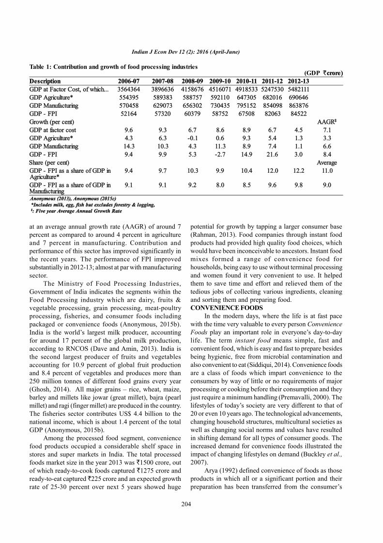
The perusal of Table 1 presented the contributionand growth of food processing industries (FPI). The foodprocessing sector forms an important segment of theIndian economy in terms of its contribution to GDP. Thesector contributed as much as 9.0 to 11.0 percent ofGDP in agriculture and manufacturing sector. During thelast 5 years ending 2012-13, FPI sector has been growing
204
Indian J Econ Dev 12 (2): 2016 (April-June)
at an average annual growth rate (AAGR) of around 7percent as compared to around 4 percent in agricultureand 7 percent in manufacturing. Contribution andperformance of this sector has improved significantly inthe recent years. The performance of FPI improvedsubstantially in 2012-13; almost at par with manufacturingsector.
The Ministry of Food Processing Industries,Government of India indicates the segments within theFood Processing industry which are dairy, fruits &vegetable processing, grain processing, meat-poultryprocessing, fisheries, and consumer foods includingpackaged or convenience foods (Anonymous, 2015b).India is the world’s largest milk producer, accountingfor around 17 percent of the global milk production,according to RNCOS (Dave and Amin, 2013). India isthe second largest producer of fruits and vegetablesaccounting for 10.9 percent of global fruit productionand 8.4 percent of vegetables and produces more than250 million tonnes of different food grains every year(Ghosh, 2014). All major grains – rice, wheat, maize,barley and millets like jowar (great millet), bajra (pearlmillet) and ragi (finger millet) are produced in the country.The fisheries sector contributes US$ 4.4 billion to thenational income, which is about 1.4 percent of the totalGDP (Anonymous, 2015b).
Among the processed food segment, conveniencefood products occupied a considerable shelf space instores and super markets in India. The total processedfoods market size in the year 2013 was `1500 crore, outof which ready-to-cook foods captured `1275 crore andready-to-eat captured `225 crore and an expected growthrate of 25-30 percent over next 5 years showed huge
potential for growth by tapping a larger consumer base(Rahman, 2013). Food companies through instant foodproducts had provided high quality food choices, whichwould have been inconceivable to ancestors. Instant foodmixes formed a range of convenience food forhouseholds, being easy to use without terminal processingand women found it very convenient to use. It helpedthem to save time and effort and relieved them of thetedious jobs of collecting various ingredients, cleaningand sorting them and preparing food.CONVENIENCE FOODS
In the modern days, where the life is at fast pacewith the time very valuable to every person ConvenienceFoods play an important role in everyone’s day-to-daylife. The term instant food means simple, fast andconvenient food, which is easy and fast to prepare besidesbeing hygienic, free from microbial contamination andalso convenient to eat (Siddiqui, 2014). Convenience foodsare a class of foods which impart convenience to theconsumers by way of little or no requirements of majorprocessing or cooking before their consumption and theyjust require a minimum handling (Premavalli, 2000). Thelifestyles of today’s society are very different to that of20 or even 10 years ago. The technological advancements,changing household structures, multicultural societies aswell as changing social norms and values have resultedin shifting demand for all types of consumer goods. Theincreased demand for convenience foods illustrated theimpact of changing lifestyles on demand (Buckley et al.,2007).
Arya (1992) defined convenience of foods as thoseproducts in which all or a significant portion and theirpreparation has been transferred from the consumer’s
Table 1: Contribution and growth of food processing industries(GDP `crore)
Description 2006-07 2007-08 2008-09 2009-10 2010-11 2011-12 2012-13GDP at Factor Cost, of which... 3564364 3896636 4158676 4516071 4918533 5247530 5482111GDP Agriculture* 554395 589383 588757 592110 647305 682016 690646GDP Manufacturing 570458 629073 656302 730435 795152 854098 863876GDP - FPI 52164 57320 60379 58752 67508 82063 84522Growth (per cent) AAGR$
GDP at factor cost 9.6 9.3 6.7 8.6 8.9 6.7 4.5 7.1GDP Agriculture* 4.3 6.3 -0.1 0.6 9.3 5.4 1.3 3.3GDP Manufacturing 14.3 10.3 4.3 11.3 8.9 7.4 1.1 6.6GDP - FPI 9.4 9.9 5.3 -2.7 14.9 21.6 3.0 8.4Share (per cent) AverageGDP - FPI as a share of GDP inAgriculture*
9.4 9.7 10.3 9.9 10.4 12.0 12.2 11.0
GDP - FPI as a share of GDP inManufacturing
9.1 9.1 9.2 8.0 8.5 9.6 9.8 9.0
Anonymous (2013), Anonymous (2015c) *Includes milk, egg, fish but excludes forestry & logging,
$: Five year Average Annual Growth Rate
205
Verma and Singh: Challenges and prospects of convenience food in India: An overview
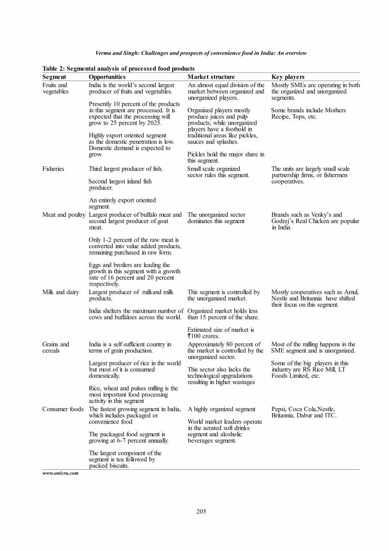
Table 2: Segmental analysis of processed food productsSegment Opportunities Market structure Key playersFruits andvegetables
India is the world’s second largestproducer of fruits and vegetables.
Presently 10 percent of the productsin this segment are processed. It isexpected that the processing willgrow to 25 percent by 2025.
Highly export oriented segmentas the domestic penetration is low.Domestic demand is expected togrow.
An almost equal division of themarket between organized andunorganized players.
Organized players mostlyproduce juices and pulpproducts; while unorganizedplayers have a foothold intraditional areas like pickles,sauces and splashes.
Pickles hold the major share inthis segment.
Mostly SMEs are operating in boththe organized and unorganizedsegments.
Some brands include MothersRecipe, Tops, etc.
Fisheries Third largest producer of fish.
Second largest inland fishproducer.
An entirely export orientedsegment.
Small scale organizedsector rules this segment.
The units are largely small scalepartnership firms, or fishermencooperatives.
Meat and poultry Largest producer of buffalo meat andsecond largest producer of goatmeat.
Only 1-2 percent of the raw meat isconverted into value added products,remaining purchased in raw form.
Eggs and broilers are leading thegrowth in this segment with a growthrate of 16 percent and 20 percentrespectively.
The unorganized sectordominates this segment
Brands such as Venky’s andGodrej’s Real Chicken are popularin India.
Milk and dairy Largest producer of milkand milkproducts.
India shelters the maximum number ofcows and buffaloes across the world.
This segment is controlled bythe unorganized market.
Organized market holds lessthan 15 percent of the share.
Estimated size of market is`100 crores.
Mostly cooperatives such as Amul,Nestle and Britannia have shiftedtheir focus on this segment.
Grains andcereals
India is a self sufficient country interms of grain production.
Largest producer of rice in the worldbut most of it is consumeddomestically.
Rice, wheat and pulses milling is themost important food processingactivity in this segment
Approximately 80 percent ofthe market is controlled by theunorganized sector.
This sector also lacks thetechnological upgradationsresulting in higher wastages
Most of the milling happens in theSME segment and is unorganized.
Some of the big players in thisindustry are RS Rice Mill, LTFoods Limited, etc.
Consumer foods The fastest growing segment in India,which includes packaged orconvenience food
The packaged food segment isgrowing at 6-7 percent annually.
The largest component of thesegment is tea followed bypacked biscuits.
A highly organized segment
World market leaders operatein the aerated soft drinkssegment and alcoholicbeverages segment.
Pepsi, Coca Cola,Nestle,Britannia, Dabur and ITC.
www.onicra.com

206
Indian J Econ Dev 12 (2): 2016 (April-June)
kitchen to the processing plant. He observed that all overthe world during the last two decades, the conveniencefood market had witnessed breath taking changes inquality and quantity of products available and thepackaging technology employed for their processing.Convenience food minimizes the working time but it doesnot save us from consuming high preservatives, extrasodium and hydrogenated fats. The study conducted byBanerjee et al. (2013) aimed to identify the factorsresponsible for awareness towards convenience foodamong women from Raipur city. Their study revealedthat 72 percent working and 94 percent non-workingwomen knew that consumption of convenience foodmight lead to obesity and cancer like diseases. Dealingwith convenience were difficult since multiplecharacteristics could contribute to the convenienceattribute of food products for example, preparationmethod and time, preservation, packaging and addedculinary skills were all characteristics which contributedto the convenience attribute of food products (Harris andShiptsova, 2007).
Priya and Mathew (2014) studied martialdissimilarities towards the consumption of conveniencefood. Their results showed that there was a significantdifference between married and unmarried respondentson the product attributes and sensory attributes and itwas observed that the behavioural, packing, healthconsequence factors of married and unmarried were notsignificantly different. Capps et al. (1985) analyzedconvenience foods based on the degree of processing oradded features and used three classifications ofconvenience food: 1) basic convenience foods, productswhere the processing was more related to preservationrather than to ease of preparation (foods with a single orlimited number of ingredients and foods with time orenergy inputs but not culinary expertise built in); 2)complex convenience foods, which encompassed multi-ingredient prepared mixtures and foods which have highlevels of time saving and energy inputs as well as culinaryexpertise built into the products; and 3) manufacturedconvenience foods, which deal with foods which haveno home-prepared counterparts. They also created a non-convenience food class composed of fresh (unprocessed)foods and home-produced, home-frozen home-cannedor home-preserved food items.
Ryan et al. (2002) revealed differences towardsconvenience orientation between six established consumersegments in the Irish population. The established groupsincluded: hedonistic food consumers (28 percent),conservative food consumers (21 percent), extremelyuninvolved food consumers (16 percent), enthusiasticfood consumers (14 percent), moderate food consumers(13 percent) and adventurous food consumers (8 percent).
It was found that the hedonistic, extremely uninvolvedand adventurous food consumers were the mostconvenience oriented out of the six groups, displayingthat differences were present between the groups’convenience-orientation. Olsen et al. (2007) investigatedcultural differences between five European countries inthe meaning of convenience orientation and the relationshipbetween convenience, attitudes and fish consumption. Itwas found that actual levels of convenience orientationdiffered from country to country. A study completed byMarquis (2005) confirmed the importance of conveniencein determining food choice among young, single adultsliving in residence halls. It was found that conveniencewas the most important food choice factor, while price,pleasure, health and concern about weight followed after.Similarly, Marquis and Manceau (2007) determined thatconvenience played a big role in determining food choicesof single men living in apartments in Montreal.
Botonaki et al. (2007) applied the model ofconvenience orientation in order to examine consumerbehaviour in the context of convenience food usage. Theirempirical results indicated that socio-demographiccharacteristics affect behaviour both directly andindirectly through perceived time resources andconvenience orientation towards meal preparation andclearing up. Even though traditionally convenience hasbeen examined in the context of strategies used by theconsumer to reduce time pressures, time is not the onlydimension involved in the consumption of conveniencefoods. Pearson et al. (1985) used preparation time as thefocal point to classify convenience foods, but alsoconsidered the use of the food in the household meal.The first component part of the categorization was adetailed system consisting of 14 categories. Those 14categories were then represented by a condensed three-category form consisting of no preparation, somepreparation and considerable preparation. Darian andCohen (1995) proposed two dimensions of convenience.The first one concerned the type of convenience, whichcould be saving time, physical energy and mental energy.The second dimension referred to the stage of the mealprocess that convenience was obtained.
The demand for convenience food has been fuelledby increased female participation in the workforce(Somogyi, 1990, Stafford and Wills, 1979). Warde (1999)emphasized that many people were constrained to eatwhat they called convenience foods as a provisionalresponse to intransigent problems of scheduling everydaylife. It was maintained that convenience food was requiredbecause people were too often in the wrong place; theimpulse to time-shifting aroused from the compulsion toplan ever more complex time-space paths in everydaylife. Brown and Mcenally (1993) suggested that it was

207
Verma and Singh: Challenges and prospects of convenience food in India: An overview
important to consider convenience at all stages in theprocess of food consumption and to determine theproportionate importance that consumers attached to timeand energy used in acquisition, consumption and disposal.Candel (2001) emphasized that there was a mental effortcomponent associated with convenience and in thecontext of meal preparation that related to the extent towhich the individual enjoyed the activity of preparingmeals. Studies have been conducted by manyresearchers, academicians, professionals and practitionerson convenience food yet there is tremendous room forresearch involving convenience foods. The present studyaimed at in-depth review of work related to changingscenario of food processing with reference toconvenience food in India.WHY CONVENIENCE FOODS?
Convenience food is gaining acceptance primarilyfrom Indian youth and is becoming part of day to day life(Srinivasan and Shende, 2015). With higher disposableincome, consumers today demand for quality and healthyfood that is offered as per their convenience and changingneeds (Jayadevan, 2012). The quality of convenience foodranges from the least expensive to the highest qualitygourmet items. Some of the economic advantages ofconvenience foods as perceived by Linstrom and Seigle(1976) are labour-saving equipment, time saving methodand reduced labour costs. With proper planning andmanagement, convenience items may reduce purchasingtime, storage facilities and food costs. Hales (2003) foundthat about 90 percent of Americans purchasedconvenience foods and nearly 25 percent used more timesaving convenience foods today than in 2001.Convenience foods require more freezer space but lesspreparation area. Faced with rising food prices, increasingwages and a lack of skilled personnel, the food serviceindustry can reduce some costs and increase efficiencyby using convenience foods. As a result of the widevariety of convenience foods, the operator can offercustomers special diet foods, such as those low incholesterol, salt, carbohydrates, or high in protein.CLASSIFICATION OF CONVENIENCE FOODS
Types of convenience foods can vary by countryand geographic region. Some convenience foods havereceived criticism due to concerns about nutritionalcontent and how its packaging may increase solid wastein landfills. Convenience foods are broadly classified intothree major categories:Ready-to-Eat (RTE) Foods: Ready-to-eat (RTE) foodsare foods intended to be consumed as they are. Thesefoods do not require additional cooking and are usuallystored in refrigeration or at room temperature (Muktawatand Varma, 2013). Goyal and Singh (2007) have exploredthat the young Indian consumer had passion for visiting
RTE outlets for fun and change but the consumeracceptability for RTE in the future would be decided onlyby the quality of food and customer service. The RTEmarket in India is expected to expand to reach 2,900crore by 2015, according to an analysis done by TataStrategic Management Group (Vijayabaskar andSundaram, 2012). In India, the convenience food industry,with a 90 percent contribution of ready-to-eat segmentin 2013 has been growing at a Compounded AnnualGrowth Rate (CAGR) of 15 percent from 2007 to 2013(Kulkarni, 2014). The consumers’ demand for RTE foodis showing consistent growth due to its convenient natureat a reasonable price and also the appeal of RTE food fortexture (Senthil et al., 2015).Ready-to-Use (RTU) Foods: Ready-to-use Foods (RTU)are highly fortified, oil-based nutrient dense pastesspecifically designed for the treatment ofmalnutrition. Patel et al. (2005) suggested thatsupplementary feeding with ready-to-use therapeutic foodpromotes better growth in children at risk of malnutritionthan the standard fortified cereal/legume-blended food.RTU foods are made from varying combinations of grains,pulses and seeds, milk powder, sugar, oil, vitamins andminerals. These foods need some preparations likecooking, frying, reconstitution, dilution etc. beforeconsumption. As they are oil-based, bacteria cannot growin ready-to-use foods which can be stored safely for upto one year without the need for refrigeration. In aresource poor setting, these products are literally life-savers (www.validnutrition.org). Thakur et al. (2013)compared the efficacy of locally-prepared ready-to-usetherapeutic food (LRUTF) and locally-prepared F100 dietin promoting weight-gain in children with severe acutemalnutrition during rehabilitation phase in hospital. Theyobserved that LRUTF promoted more rapid weight-gainwhen compared with F100 in patients with severe acutemalnutrition during rehabilitation phase.Beverages: Beverages are potable drinks which havethirst-quenching, refreshing, stimulating and nourishingqualities and they are specifically prepared for humanconsumption. Wolf et al. (2008) have demonstrated thatbeverages containing sugar, high fructose corn syrup(HFCS) or alcohol are handled differently by the bodythan when sugar or HFCS are incorporated in solidfoods. Increased sugar-sweetened beverages intake isassociated with weight gain and obesity (Malik et al.,2006). Beverages are broadly classified into alcoholicbeverages and non-alcoholic beverages. An alcoholicbeverage is a drink containing ethanol, commonly knownas alcohol. Current trends suggested increasinginvolvement of the alcoholic beverage industry in scientificresearch in ways that go beyond investigating the productsafety and consumer marketing (Babor, 2009). Non-

208
Indian J Econ Dev 12 (2): 2016 (April-June)
alcoholic beverage is a beverage that contains no alcohol.Such drinks are generally drunk for refreshment, or toquench people’s thirst. India is the third largest marketof alcoholic beverages.The beverages were estimated atUS$ 155 million out of which fruit juices and fruit-baseddrinks constituted US$ 60 million (Chetty, 2012).
SEASONINGS, KEY TO TASTY CONVENIENCEFOODS
The key to tasty and appetizing convenience foodsis the seasonings added to them. Seasoning is acomprehensive term applied to aromatic ingredients thatimprove the flavor of food products. These arecompounds, containing one or more spices, or spiceextractives, which when added to a food during itsmanufacturing, preparation or before it is served, enhancethe natural flavor of the food and increase its acceptanceby consumers (Farrell, 1998). Despite the limited use ofspices and seasonings in food, their impact on foodprocessed, stored or packaged is immense. If used in theright quantity, it is beneficial to health but then excessuse may result in harmful effects (Gadegbeku et al.,2014). Spices, herbs and dried vegetable seasonings arecurrently treated with ionizing radiation to eliminatemicrobial contamination (Khan and Abrahem, 2010).Proper seasoning is an art. With a little patience this art iseasy to learn and adapt. There are no hard-and-fast rulesfor the use of seasoning; however Thorner (1973) gavethree basic practices that should be followed: (1) underseason, rather than over season, because it is difficult toreduce the seasoning level without injuring the product;(2) experiment with various seasonings and becomefamiliar with the seasonings that are available; (3) useonly fresh, high-quality seasonings.MARKET SIZE OF CONVENIENCE FOODINDUSTRY IN INDIA
The total value of Indian food processing industrywas around US$12 billion in 2012 and was expected tobe around US$194 billion by 2015. According to theAgricultural & Processed Food Products ExportDevelopment Authority (APEDA), India’s agricultural andprocessed food exports stood at US$18.65 billion duringApril 2012-March 2013, which was US$13.22 billion lastyear. The Indian food processing sector employed over10 million people with total investment of US$24.04 billiongrown at 20 percent per annum in the last five years(Kulkarni, 2014). Demand for convenience foodsproducts in India remains need-based. Hence, productssuch as dairy and oil which form part of the daily stapledominate the total convenience food consumption.
Major players in the convenience food sector areNestle, Parle Agro, Britannia, Cadbury, MTR, KwalityDairy and ITC-Agro. The demand for convenience food
has increased manifold in past 2 years, according to asurvey conducted by Associated Chambers of Commerceand Industry of India (ASSOCHAM). The surveyindicated annual growth of about 40-60 percent between2011 and the end of 2015 for the convenience and ready-to-eat food segments. Growing at a compounded annualgrowth rate (CAGR) of about 15 to 20 percent annually,the Indian convenience food industry is likely to touch$30 billion by 2015 from the current level of $15 billionincluding snack foods, ready-to-eat foods, healthy andfunctional foods (Thomas and Pant, 2012).
THE RISE OF THE CONVENIENCE FOOD MARKETIN INDIA
Our ways of cooking have changed since morehouseholds are experiencing drastic change in eatinghabits and meals need to be prepared as quickly andconveniently as possible in order to keep up with the paceof life. There are various reasons which have graduallyresulted in the rise of convenience food in the country.These are:Pre-packaged Items: This is where convenience foodhas begun to fill the gap. More and more people now aredependent on convenience food as well as pre-packageditems to help them facilitate their day to day activity. Theconvenience food products are often sold in portioncontrolled, single serve packaging designed for portability.Then there are some packaged mixes which require somepreparation and cooking either in the oven or on the stovetop. Nutrition labelling on food products has emerged asa prominent policy tool for promoting healthy eating(Cowburn and Stockley, 2005). Therefore, nutrition labelson pre-packaged foods are among the most prominentsources of information (Campos et al., 2011) althoughingredients and health claims may be perceived as moreimportant (Reid and Hendricks, 1993).On-The-Go Lifestyle: The food-related lifestyledeterminants have been identified as important whenconsidering the convenience food purchasing patterns (DeBoer et al., 2004). Convenience foods are perceived toinvolve a lower degree of planning and preparation (Bogueand Sorenson, 2001). On-the-go lifestyles have emergedas a result of several factors, longer working hours, longercommuting times and a wider range of leisure activities,thus a family is less inclined to spend what valuable timeit has on preparing food. The main consequence of thishas been a greater reliance on ready-prepared foods inthe evening. Gofton (1995) suggested that in dual-incomehouseholds the family is often served convenience foodswhen parents are too tired and/or do not have enoughtime to prepare a home cooked meal.Mall Culture or Supermarkets: The supermarkets arecreating an environment of impulsive buying where most

209
of the convenience foods packed in their full splendourand tagged with hot offers lure the customers to try them.The entry of global supermarket chains into developingcountries has been an important factor behind theexpansion of the supermarket network and the increasedpresence of supermarkets in food markets (Arda, 2006).Emergence of mall culture has led to increase incompetition in the food retail supermarket industry(Mohan, 2013). Large-scale food manufacturers haveincreased their importance in the food system assupermarkets and have similar and indeed related impactsupstream in the food system’ (Reardon and Berdegué,2002).Packaging: One of the main reasons for the growth ofconvenience food is the packaging that comes with itand it serves a very important role to market conveniencefood products and improves their usefulness (Onyebuchi,2013). The packaging systems are now being designedkeeping environmental aspects in mind and there are eco-friendly packaging materials in the market that arerecyclable and biodegradable. McDaniel and Baker (1977)speculated that the consumers perceived a higher qualityof product in the more expensive packaging and they arewilling to sacrifice the ease of opening in order to obtaina higher quality. Further, packaging systems are designedkeeping storage aspects in mind and therefore we havezipper pack in the market, which is re-closable afteropening up the pack. There are also composite containerswith foil lining to keep the product fresh inside, whichcan replace conventional tin containers in the market.OPPORTUNITIES FOR THE CONVENIENCE FOODMARKET IN INDIA
Convenience food is a concept that is prevalent inthe developed world since long, while its inception intothe Indian market has been recent. According to Chadhaet al. (2010), the opportunities that fuel the Indianconvenience food market are:Changing Demographics of the Indian Population:The Indian population is younger, more urban, with greaterdisposable income and high purchasing power parity(PPP). Blaylock (1999) showed that a rise in incomehad a positive effect on food choice. Urban consumersare typically busier and more affluent, thus more willingto pay for convenience. The main impact of urbanizationhas created a growing demand for convenient products.Ready meals thus saw a strong 18 percent growth in2008 over the previous year, with these products regardedas a convenient alternative to cooking from scratch.Packaged soup also benefited, with dehydrated soupgrowing by 21 percent in current value terms, whileinstant noodles became an increasingly popular snack ormeal component, with sales thus growing by 24 percent.Veenma et al. (1995) assessed the significance of psycho-
social, demographic and life-style factors using acovariance structure model. Their results indicated thatthe most important determinants of convenience foodusage were nutritional knowledge, socio-economic status,marital status, employment status and stage in the familylife cycle.Convenience: It is evident that convenience plays aprominent role in the food choices of today’s customers.Wales (2009) suggested that food products offering lessconvenience are deemed to be less preferable toconsumers. The growing presence of drive-thruwindows, microwave dinners, take-out meals, homedelivery for groceries and internet shopping, alldemonstrate the importance of convenience in determiningfood choices (Jaeger and Cardello, 2007). Jaeger andMieselman (2004) investigated the construct of food-related convenience itself, looking over each stage of themeal preparation process. Scholderer and Grunert (2004)discovered that convenience includes dimensions of bothtime and effort saving. Verlegh and Candel (1999)investigated the situational influence as another dimensionof food related convenience and found that ‘socialsituations’ impacted the intention of consumers’consumption of convenience foods. Berry et al. (2002)indicated that convenience consumption has beenoperationalized by the use of convenience foods (frozenexpensive entrees, ready-to-eat cold cereal) and timesaving durables (microwave oven, dishwasher andfreezer).Nutritional and Health Benefits: The concept thatcertain foods can promote health by aiding in theprevention or treatment of disease, is increasingly gainingacceptance within the public arena and the scientificcommunity (Winter and Rodriguez, 1997). According tothe research conducted by Weaver et al. (2014), nutritionscientists, public health professionals, agriculturaleconomists, food scientists and other professionalsdedicated to meet the food and nutritional needs of peoplearound the globe recognized that fresh, local foods couldnot meet all nutritional requirements. Birch (1999) hasonly a rudimentary understanding of factors that promotethe development of food preferences consistent withhealthy diets and optimal nutrition. According to Dixonet al. (2006), consumers were being encouraged toembrace convenient food solutions, while also beingconcerned about the nutritional qualities of foods. Manyfood producers communicated that their products werepart of a healthy diet or claimed that they provided specifichealth benefits to inform the consumer through nutrientlabels and front-of-package labeling (McGuire, 2012).EMERGING NEW CATEGORIES OF CONVENIENCEFOOD IN INDIA
According to Agrawal, 2011, the emerging new
Verma and Singh: Challenges and prospects of convenience food in India: An overview
210
Indian J Econ Dev 12 (2): 2016 (April-June)
categories and the future of convenience food in Indiaare:Value-added Dairy Products: The dairy productssegment constitutes about 35 percent of the totalconvenience food industry in India. The main growthdrivers in this segment are curd, ghee and ice creams.Dairy product demand is anticipated to grow in the nextfive years by some 15-20 percent. Abdulla (2014) saidthat cheese and yoghurt offered a very good opportunityespecially when consumers had become more willing tospend on value-added dairy products. The IndianGovernment has been focusing on the dairy industry toothrough policy support with major supportive initiativeslike: In the sector of dairy processing, 51 percent offoreign equity participation is permitted. A recent reportby CARE Ratings said that the significant transformationtook place in the Indian demographic space which led toheightened consumer interest in Value-added DairyProducts. According to estimates, the share of Value-added Dairy Products in the milk and milk derivativessegment was growing at about 25 percent every yearand it was expected this pace would be maintained till2019-2020 (Das, 2014).Health-focused Snack Foods: Snack foods have beena long-time favorite in the Indian diet and now packagedand branded variants of namkeen, sweets and wafershave become the natural solution to the culinary cravingsinduced by the modern Indian lifestyle (Wanduragala,2012). Brown and Oqden (2004) compared the modellingand control theories of parental influence on children’seating attitudes and behaviour with a focus on snackfoods. His results showed that children whose parentsindicated greater attempts to control their child’s dietsreported higher intakes of both healthy and unhealthy snackfoods.
Ever increasing health consciousness gives a widermarket for snack foods which are health focused innature. Many of the large existing companies like ITCFoods, Parle Agro and Frito Lay, have considered thisfact and focused on this segment by targeting customersby offering a product line in health focused segment.Mclntyre and Baid (2009) analyzed that many adultsshowed some concerns about specific diet and healthrelated aspects of many snack products and would liketo be tempted by healthier versions. With the boostingdemand for healthy foods, this segment will witness ahuge share in snack food industry.Frozen Ready-to-eat Segment: The availability of frozenfoods in the Indian market has brought about great changein the life-style of the people of India. Among the differentreasons for the popularity of frozen foods in India, theimproving standard of living of the middle-income groupedpeople in India has also contributed towards the
development of companies in the frozen food industry inIndia (Raghu and Radha, 2013). As the penetration oforganized retail has improved, it is expected that therewill be a significant rise in the frozen ready-to-eat segment.Due to lack of cold chain facility, frozen food productswere wasted but with improved supply chain quality, theopportunities would be many (Rathore et al., 2010). It isexpected that freezer space will be doubled in the coming4-5 years, increasing the accessibility of frozen productsin the Indian market. The growth of this market will beaided by the entrance of enormous multinationalcompanies such as McCain, Tyson Foods, etc.Non-vegetarian Processed Foods: Presently, In Indiamajority of non-vegetarian products that are sold are inraw form which is unhygienic. Given the increasing needfor convenience and increasing health consciousness,considerable development in the category of nonvegetarian food is anticipated. The increasing penetrationof supermarkets/hypermarkets and improvement in coldchain infrastructure will significantly aid the growth ofthis segment. The Indian convenience food segment isnow at a very budding stage. Changes on the generalmarket, affecting demand and supply side such asincreasing urbanization, need for convenience, healthconsciousness, increased penetration of organized retailand entry of international players are key drivers that willresult in significant growth in the market.CHALLENGES FOR THE CONVENIENCE FOODINDUSTRY IN INDIA
Despite the strong growth, various regulatory andinfrastructural issues inhibit the growth of the Indianconvenience food industry. The main challenge is to retainthe nutritional value, aroma, flavour and texture of foods,and presenting them in near natural form with addedconveniences. Convenience foods need to be offered tothe consumer in hygienic and attractive packaging and atlow incremental costs (Harchekar, 2008). Key challengesfor the Indian convenience food industry are:Varied tastes and preferences: India is a country of aunique culture and has its own tastes and preferenceswhich again differ from region to region. Hence, it is achallenge for manufacturers to customise their productportfolio to local tastes and preferences rather than justbringing in global products into India.Strong unorganised market: All the key sectors of thefood industry face a stiff challenge from the unorganisedmarket. Success of the unorganised market is largely dueto easy accessibility and cheaper prices of products.Higher prices: Although convenience food products aretraditionally higher than the unorganised food market,increase in raw materials has led to further price rise inthe convenience food products.Poor infrastructure: Many categories in the convenience
211
food industry such as ready-to-eat products and frozenfood require strong infrastructural support such as coldchains and warehouses and dedicated logistic supply chainwhich is still not available in greater part of the country.CONCLUSIONS
The study revealed that the food-processing industryis significant for India’s development because it hasimportant link and synergy with industry and agriculture,the two main support of the economy. It widely comprisesof the various segments viz. fruits and vegetables, milkand milk products, poultry, packaged or convenience foodetc. Convenience foods are identified as those that arefully or partially prepared foods in which a significantamount of preparation time, culinary skills, or energyinputs have been transferred from the home kitchen tothe food processor and distributor. Convenience food isthe result of modern technological advances in the fieldof food processing, preservation techniques and theinvention of various new food additives. Its products arealways available, ready to use and properly stored butthey often contain a lot of fat and their energy content isalso very high. There is a greater demand for RTE foodsegments and the major attraction for these products isconvenience, availability and less time consumption tocook.
Ready-to-use products are free from bacteria andsafer than fresh goods, the shelf-life is longer, modernproduction techniques and preservation methods minimizethe nutritional loss of pre-cooked food products. Inregards to the dimensions of convenience, conveniencehas been defined to include aspects of both time and effortsaving - effort consisting of both physical and mentaleffort. As the customers are educated in present era theyfocus on consuming hygienic and healthy food products.Convenience foods contribute to both food security(ensuring that sufficient food is available) and nutritionsecurity (ensuring that food quality meets human nutrientneeds). The changing lifestyles and culture continue todrive the demand for convenience foods. Despite thestrong growth, various infrastructural issues and logisticsupply chain inhibit the growth of the Indian conveniencefood industry. The results of this study seem to be ofparticular interest not only for food product marketers,but also for food policy makers to understand the role ofconvenience food in India.REFERENCESAbdulla, H. 2014. Dairy in India: How to win over Indian
consumer. Culled from www.just-food.com/management-briefing/how-to-win-over-the-indian-consumer_id127988.aspx
Agrawal, N. 2011. Marketing strategies by packaged foodcompanies in India. M.Sc. Thesis, submitted to AstonBusiness School, England.
Anonymous. 2013. State of Indian Agriculture. Departmentof Agriculture and Cooperation, Ministry of Agriculture,Government of India, New Delhi.
Anonymous, 2014. Annual Report. Ministry of FoodProcessing Industries, Government of India, New Delhi.
Anonymous. 2015a. Importance of food processing sectorin India-A CII and Rabo equity report. Confederationof Indian Industry, New Delhi.
Anonymous. 2015b. A brief report on food processing sectorin India. Corporate Catalyst India, New Delhi.
Anonymous. 2015c. Data bank on economic parameters ofthe food processing sector. Ministry of Food ProcessingIndustries, Government of India, New Delhi.
Arda, M. 2006. Food retailing, supermarkets and foodsecurity: Highlights from Latin America. UNU- WorldInstitute for Development Economics Research. 107 (9):1-19.
Arya, S. S. 1992. Convenience foods- Emerging scenario.Indian Food Industry. 11 (4): 31-42.
Babor, T.F. 2009. Alcohol research and the alcoholic beverageindustry: Issues, concerns and conflicts of interest.Addiction.104 (1): 34-47.
Banerjee, S., Joglekar, A., and Kundle, S. 2013. Consumerawareness about convenience food among working andnon-working women. International Journal of ScientificResearch. 2 (10): 1-4.
Berry, L.L., Seiders, K., and Grewal, D. 2002. Understandingservice convenience. Journal of Marketing. 66 (4): 1-17.
Birch, L.L. 1999. Development of food preferences. AnnualReview of Nutrition. 19:41-62.
Blaylock, J. 1999. Economics, food choice and nutrition. FoodPolicy. 24 (2-3): 269-286.
Bogue, J. and Sorenson, D. 2001. An exploratory study ofconsumers’ attitude towards health-enhancing foods.Culled from www.ucc.ie
Botonaki, A., Natos, D., and Mattas, K. 2007. Exploringconvenience food consumption through a structuralequation model. In: Mediterranean Conference of Agro-Food Social Scientists, Spain: 1-18.
Brown, L.G. and Mcenally, M.R. 1993. Convenience:Definition, structure and application. Journal ofMarketing Management. 2 (2): 47-56.
Brown, R. and Oqden, J. 2004. Children’s eating attitudesand behaviour: a study of the modelling and controltheories of parental influence. Health EducationResearch. 19 (3): 261-271.
Buckley, M., Cowan, C., and McCarthy, M. 2007. Theconvenience food market in Great Britain: Conveniencefood lifestyle (CFL) segments. Appetite. 49 (3): 600-617.
Campos, S., Doxey, J., and Hammond, D. 2011. Nutrition labelson pre-packaged foods: A systematic review. PublicHealth Nutrition. 14 (8): 1496-1506.
Candel, M.J.J.M. 2001. Consumers’ convenience orientationtowards meal preparation: Conceptualization and
Verma and Singh: Challenges and prospects of convenience food in India: An overview

212
Indian J Econ Dev 12 (2): 2016 (April-June)
measurement. Appetite. 36 (1): 15-28.Capps, O., Tedford, J.R., and Havelicek, J. 1985. Household
demand for convenience and non-convenience foods.American Journal of Agricultural Economics. 67 (4):862-869.
Chadha, R., Bhatiani, R., and Dutta, S. M. 2010. Opportunitiesin the packaged food market in India. Technopakperspective. 3: 83-89.
Chetty, P. 2012. Major segments in India’s food processingsector. Culled from www.projectguru.in/publications/major-segments-in-indias-food-processing-sector/
Cowburn, G. and Stockley, L. 2005. Consumer understandingand use of nutrition labeling: A systematic review. PublicHealth Nutrition. 8 (1): 21-28.
Darian, J.C. and Cohen, J. 1995. Segmenting by consumertime shortage. Journal of Consumer Marketing. 12 (1):32-44.
Das, S. 2014. Dairies focus on value-added products for futuregrowth. Culled from http://www.business-standard.com/article/markets/dairies-focus-on-value-added-products-for-future-growth-114071900690_1.html
Dave, R. and Amin, A. 2013. Indian processed food: Recenttrends and future prospects. International Journal ofResearch in Business Management. 1 (1): 11-18.
De Boer, M., McCarthy, M., Cowan, C., and Ryan, I. 2004.The influence of lifestyle characteristics and beliefsabout convenience food on the demand for conveniencefoods in Irish market. Food Quality and Preference. 15:155-165.
Dixon, J.M., Hinde, S.J., and Banwell, C.L. 2006. Obesity,convenience and phood. British Food Journal. 108 (8):634-645.
Farrell, K.T. 1998. Spices, Condiments, and Seasonings.Aspen Publishers, Inc., New York
Gadegbeku, C., Tuffour, M.F., Katsekpor, P., and Atsu, B.2014. Herbs, spices, seasonings and condiments usedby food vendors in Madina, ACCRA. CaribbeanJournal of Science and Technology. 2: 589-602.
Ghosh, N. 2014. An assessment of the extent of foodprocessing in various food sub-sectors. Culled fromwww.iegindia.org/ardl/2014-11-n-1.pdf
Gofton, L. 1995. Food choice and the consumer. BlackieAcademic and Professional, Glasgow, United Kingdom.
Goyal, A. and Singh, N.P. 2007. Consumer perception aboutready-to-eat in India: An exploratory study. British FoodJournal. 109 (2): 182-195.
Hales, D. 2003. What (and who) is really cooking at yourhouse. Culled from http://www.utexas.edu/courses/stross/ant393b_files/ARTICLES/americaeats.htm
Harchekar, N. 2008. Indian processed food industry-Opportunities Galore. Culled fromwww.way2wealth.com/reports/RR150420084.PDF
Harris, J.M. and Shiptsova, R. 2007. Consumer demand forconvenience foods: Demographics and expenditures.Journal of Food Distribution Research. 38 (3): 22-36.
Jaeger, S.R. and Cardello, A.V. 2007. A construct analysis ofmeal convenience applied to military foods. Appetite.49 (1): 231-239.
Jaeger, S.R. and Meiselman, H.L. 2004. Perceptions of mealconvenience: The case of at home evening meals.Appetite. 42 (3): 317-325.
Jayadevan, G.R. 2012. Ethics and marketing of processedfoods in India. Abhinav National Journal of Researchin Commerce & Management. 1 (12): 8-15.
Khan, A. and Abrahem, M. 2010. Effect of irradiation on qualityof spices. International Food Research Journal. 17 (4):825-836.
Kulkarni, S. 2014. CAGR of convenience food market 15%and tetra pack preferred packaged material. Culled fromwww.fnbnews.com.
Linstrom, H.R. and Seigle, N. 1976. Convenience foods forthe hotel, restaurant and institutional market: Theprocessor’s view. National Economic Analysis Division,Economic Research Service, U.S. Department ofAgriculture, Washington, D.C.
Malik, V.S., Schulze, M.B., and Hu, F.B. 2006. Intake of sugar-sweetened beverages and weight gain: a systematicreview. The American Journal of Clinical Nutrition. 84(2): 274-288.
Marquis, M. 2005. Exploring convenience orientation as afood motivation for college students living in residencehalls. International Journal of Consumer Studies. 29(1): 55-63.
Marquis, M. and Manceau, M. 2007. Individual factorsdetermining the food behaviours of single men living inapartments in Montreal as revealed by photographs andinterviews. Journal of Youth Studies. 10 (3): 305-316.
McDaniel, C. and Baker, R.C. 1977. Convenience foodpackaging and the perception of product quality. Journalof Marketing. 41 (4): 57-58.
McGuire, S. 2012. Front-of-Package Nutrition Rating Systemsand Symbols: Promoting Healthier Choices. TheNational Academies Press, Washington, DC, USA.
Mclntyre, C. and Baid, A. 2009. Indulgent snack experienceattributes and healthy choice alternatives. British FoodJournal. 111 (5): 486-497.
Mohan, R. 2013. To identify the factors impacting customersatisfaction in food retail supermarkets. InternationalJournal of Research and Development- A ManagementReview. 2 (2): 51-54.
Muktawat, P. and Varma, N. 2013. Impact of ready to eat foodtaken by single living male and female. InternationalJournal of Scientific and Research Publications. 3 (11):1-3.
Olsen, S., Scholderer, J., Brunsø, K., and Verbeke, W. 2007.Exploring the relationship between convenience and fishconsumption: A cross-cultural study. Appetite. 49 (1):84-91.
Onyebuchi, N.J. 2013. Production, Characterization andshelf-life studies of Irvingia Gabonensis based ‘Ready-

213
to-prepare soup’. M.Sc. Thesis, submitted to Universityof Ibadan, Nigeria.
Patel, M.P., Sandige, H.L., Ndekha, M.J., Briend, A., Ashorn,P., and Manary, M.J. 2005. Supplemental feeding withready-to-use therapeutic food in Malawian children atrisk of malnutrition. Journal of Health, Population andNutrition. 23 (4): 351-357.
Pearson, J.M., Capps, O., Gassman, C., and Axelton, J. 1985.Degree-of-readiness classification system for foods:Development, testing and use. Journal of ConsumerStudies and Home Economics. 4: 249-255.
Premavalli, K.S. 2000. Convenience foods for defence forcesbased on traditional Indian foods. Defence ScienceJournal. 50 (4): 361-369.
Priya, G.B.S. and Mathew, A. 2014. A study on martialdissimilarity towards processed convenience food.ZENITH International Journal of MultidisciplinaryResearch. 4 (12): 222-232.
Raghu, G. and Radha, S. 2013. The market potential of frozenfood products in Bangalore. Social Science ResearchNetwork. (9): 1-29.
Rahman, T. 2013. RTE and RTC foods-A new era in theprocessed food industry with special reference to MTR.International Journal of Management and SocialSciences Research. 2 (5): 63-67.
Rais, M., Acharya, S., and Sharma, N. 2013. Food processingindustry in India: S&T capability, skills and employmentopportunities. Journal of Food Processing &Technology. 4 (9): 2-13.
Rathore, J., Sharma, A., and Saxena, K. 2010. Cold chaininfrastructure for frozen food: A weak link in Indian retailsector. The IUP Journal of Supply Chain Management.7 (1&2): 90-103.
Reardon, T. and Berdegué, J. 2002. The rapid rise ofsupermarkets in Latin America: Challenges andopportunities for development. Development PolicyReview. 20 (4): 371-388.
Reid, D.J. and Hendricks, S. 1993. Consumer awareness ofnutrition information on food package labels. Journalof Canadian Dietetic Association. 54 (3): 127-131.
Ryan, I., Cowan, C., McCarthy, M., and O’Sullivan, C. 2002.Food-related lifestyle segments in Ireland with aconvenience orientation. Journal of International Food& Agribusiness Marketing. 14 (4): 29-47.
Scholderer, J. and Grunert, K.G. 2004. Consumers, food andconvenience: The long way from resource constraintsto actual consumption patterns. Journal of EconomicPsychology. 26 (1): 105-128.
Senthil, A., Kumar, B.S., and Pathak, A. 2015. Comparativequality evaluation of commercial extruded snacks.Wudpecker Journal of Food Technology. 3 (1): 1-11.
Siddiqui, A. 2014. Study to evaluate the preferences ofworking women and housewives towards packaged andnon packaged food. Abhinav National Journal ofResearch in Commerce & Management. 3 (6): 1-6.
Singh, H. and Bansal, M. 2013. Major problems and prospectsof food processing industry in Punjab. InternationalJournal of Management Excellence. 1 (1): 7-12.
Singh, S.P., Tegegne, F., and Ekenem, E. 2012. The foodprocessing industry in India: Challenges andopportunities. Journal of Food Distribution Research.43 (1): 81-89.
Somogyi, J.C. 1990. Convenience foods and the consumer-Current questions and controversies. NutritionalAdaptation to New Lifestyles. 45: 104-107.
Srinivasan, S. and Shende, K.M. 2015. A study on the benefitsof convenience foods to working women. ATITHYA: AJournal of Hospitality. 1 (1): 43-50.
Stafford, T.H. and Wills, J.W. 1979. Consumer demandincreasing for convenience in food products. NationalFood Review. 13: 15-17.
Thakur, G.S., Singh, H.P., and Patel, C. 2013. Locally-preparedready-to-use therapeutic food for children with severeacute malnutrition: A controlled trial. Indian Pediatrics.50 (3): 295-299.
Thomas, T. and Pant, S. 2012. Rise of convenience food-Impact on the industry. Culled from http://www.fnbnews.com.
Thorner, M.E. 1973. Convenience and Fast food handbook.The AVI Publishing Company, Inc., Westport,Connecticut
Veenma, K.S., Kistemaker, C., Lowik, M.R.H., Hulshof,K.F.A.M., Steerneman, A.G.M., and Wedel, M. 1995.Socio-demographic, psycho-social and life-style factorsaffecting consumption of convenience food. EuropeanAdvances in Consumer Research. 2: 149-156.
Verlegh, P.W.J. and Candel, M.J.J.M. 1999. The consumptionof convenience foods: Reference groups and eatingsituations. Food quality and preference. 10 (6): 457-464.
Verma, S. 2015. Role of agro-industries for sustainableagricultural development in India. Indian Journal ofEconomics and Development. 11 (1): 277-284.
Vijayabaskar, M. and Sundaram, N. 2012. A market study onkey determinants of ready-to-eat/cook products withrespect to Tier-1 cities in southern India. InternationalJournal of Multidisciplinary Research. 2 (6): 168-180.
Wales, M.E. 2009. Understanding the role of convenience inconsumer food choices: A review article. Studies byUndergraduate Researchers at Guelph. 2 (2): 40-48.
Wanduragala, G. 2012. Strategies for success in India’s snackfood market. Culled from http://kanvic.com.
Warde, A. 1999. Convenience food: Space and timing. BritishFood Journal. 101 (7): 518-527.
Weaver, C.M., Dwyer, J., Fulgoni, V.L., King, J.C., Leveille,G.A., MacDonald, R.S., Ordovas, J., and Schnakenberg,D. 2014. Processed foods: Contributions to nutrition.The American Journal of Clinical Nutrition. 99 (6):1525-1542.
Winter, K. and Rodriguez, G. 1997. Consumers’ views on
Verma and Singh: Challenges and prospects of convenience food in India: An overview

214
Indian J Econ Dev 12 (2): 2016 (April-June)
nutrition and public health. Proceedings of the NutritionSociety. 56 (3): 879-888.
Wolf, A., Bray, G.A. and Popkin, B.M. 2008. A short history ofbeverages and how our body treats them. ObesityReviews. 9 (2): 151-164.
Webliographywww.makeinindia.comwww.onicra.comwww.validnutrition.org

215
Indian Journal of Economics and DevelopmentVolume 12 No.2: 216-222
April-June, 2016DOI: 10.5958/2322-0430.2016.00128.1
www.soed.in
Domestic Water Consumption Pattern and its Linkage withSocio-economic Variables: A Case Study of Ludhiana City
Jasdeep Kaur1*, A.S. Bhullar2, and R.S. Ghuman3
1Kamla Lohtia Sanatan Dharam College, Daresi, Ludhiana- 1410082Economics Program, University of Northern British Columbia, BC, Canada3Nehru SAIL Chair Professor, CRRID, Chandigarh-160019
*Corresponding author’s email: [email protected]
Received: January 07, 2016 Accepted: May 08, 2016
ABSTRACTThe consumption of water depends on the life style of the population, work and working conditions, climate, culture andfood habits etc. The per household and per capita water consumption in the selected households of the Ludhiana cityshowed that high income groups consume more water than the low income and slum households. The relationshipbetween demographic and socio-economic variables like education, occupation and household income and waterconsumption was positive. The paper reviews the domestic water consumption pattern and its linkage with socio-economicvariables in Ludhiana city.
KeywordsDeficiency, education, income, , occupation, water consumption
JEL CodesI25, P46, Q25, R21
INTRODUCTIONWater, the basic need of life, is likely to surpass the
scarcity of many other commodities during the twenty-first century. It will be a great challenge to meet increaseddemand for water due to increasing population, economicgrowth and technological changes. The opportunities toenhance the supply of potable water are becomingincreasingly limited (Marothia, 2003). The supply isshrinking year by year due to over exploitation, pollutionand inefficient water use methods and policies. This ismore so in the developing countries due to uncheckedpopulation growth, interest groups competition andconflict (Ballabh, 2003), expansion of economic activities(Biswas, 1993 and Narayanamoorthy, 2003) along withlack of institutional framework and policies for watermanagement. It is certain that coming generations haveto confront, among other things, demographic transitionof population, geographical shift of population,technological advancement, growing globalization,degradation of the environment and the emergence ofwater scarcity.
The quantity of water consumed in most of the
Indian cities is not determined by the demand but thesupply. People attempt to adjust to the quantity as well asquality of water supplied. A majority of households inmajor cities in India depend on the municipal water supplyfor their daily needs (Anonymous, 2010).
There are lots of asymmetries in the household waterconsumption. The water consumption varies acrosslocalities, household sizes, income and occupationalcategories, demographic profiles etc. These variations inthe water consumption, by and large, are the sum totalof activity-wise water use differentials.
This paper endeavors to examine the domestic waterconsumption pattern in Ludhiana city of Punjab. Thepaper has been divided into five sections. Section I dealswith the database and methodology of the study. The perday water consumption norms suggested in various plandocuments and by other organizations have been enlistedin the Section II. In Section III, an effort has been madeto examine the locality-wise, activity-wise and season-wise per household and per capita water consumption.Section IV deals with the relationship between the socio-economic and demographic variables. The summary and

216
Indian J Econ Dev 12 (2): 2016 (April-June)
conclusions have been presented in the last section.DATABASEAND METHODOLOGY
This paper is mainly based on primary data collectedthrough a survey of the households by personal interviewmethod. To examine the pattern of water consumption,cross sectional data from 360 households was collectedthrough a questionnaire. The data pertains to the year2009-10. The different localities of Ludhiana city werecategorized into six income clusters1 as following:1. Very High Income Group (VHIG) areas with well-
planned localities and buildings and the plot size morethan 400 square yards.
2. High Income Group (HIG) areas with well-plannedlocalities and buildings and the plot size varyingbetween 250 to 400 square yards.
3. Middle Income Group (MIG) areas with well-plannedlocalities and buildings and the plot size varyingbetween 125 to 250 square yards.
4. Low Income Group (LIG) areas with well-plannedlocalities and buildings and the plot size less than 125square yards.
5. Mixed areas2
6. Slum areasIn this way, a number of clusters falling under each
income group were identified. Four localities from eachincome cluster were selected and from each locality 15respondents were interviewed. Thus the total number ofhouseholds surveyed from each cluster was 60. In thisway, the total sample included 360 households from 6income clusters. From the selected households the dataregarding plot size, household income, occupationstructure, and education level of the head of the householdwere collected and analyzed so as to examine therelationship of these variables with water consumption.
The data were collected through a structured scheduleby recall method and the target respondents werehousewives. The volume of vessels in which householdsstore water was assessed and the number of vessels ofwater used in different activities like bathing, clotheswashing, utensil cleaning, house cleaning, watering thelawn and pots etc. were estimated. The quantity of watercontained in the vessels was assessed by physicallymeasuring the quantity of water contained in a vessel. Apilot survey of ten houses using different kind of vessels
was conducted for this purpose. In this way, the averagesize of the vessel was assessed and this average wasused to work out the quantity of water used for differentactivities. The average size of the vessel was 9.73 liters.
Where running tap or piped water was used in someactivities, the duration for which the tap was used wasestimated and the quantity of water delivered per minutefrom the tap was measured. The quantity of water usedin flushing toilet was measured by volume of bucket usedand flush tank capacity.RESULTSAND DISCUSSIONWater Requirement Norms and Standards
A number of factors like climate, culture, food habits,work, and working conditions, level and type ofdevelopment and physiology determine the requirementof water. The World Health Organization (WHO, 2003)classifies the supply and access to water in four servicecategories. These categories are:i. No Access (Water available below 5 lpcd)ii. Basic Access (Avg. app. 20 lpcd)iii. Intermediate Access (Avg. app. 50 lpcd)iv. Optimal Access (Avg. app. 100-200 lpcd)
The National Commission on Urbanization (1988)recommended that a per capita water supply of 90-100liters per day is needed to lead a hygienic existence andemphasized that this level of water supply must be ensuredto all citizens.
As per the Bureau of Indian Standards, IS: 1172-1993 a minimum water supply of 200 liters per capitaper day (lpcd) should be provided for domesticconsumption in cities with full flushing systems. IS: 1172-1993 also mentions that the amount of water supplymay be reduced to 135 lpcd for the LIG and theeconomically weaker sections of the society and in smalltowns.
The Ninth Plan (1997-2002) had advocated therequirement of water in urban areas as 125 lpcd in citieswith planned sewerage systems; 70 lpcd in cities withoutplanned sewerage systems; 40 lpcd for those collectingwater from public stand posts.
However, in the tenth plan (2002-2007), the citieswith planned sewerage systems were classified into twogroups based on population that is, metropolitan or megacities and non-metropolitan cities. In the former, therecommended water supply level was 150 lpcd, and inthe latter it was 135 lpcd (Anonymous, 1997-2002).
Twelfth Plan (2012-17) has set the objective toprovide 40 lpcd piped drinking water supply to 50 percentof rural population and 50 percent Gram Panchayats willachieve Nirmal Gram Status by the end of the TwelfthFive Year Plan.
Notwithstanding the IS: 1172-1993 and the five yearplan recommendations, almost every municipal
1 In a similar study Shaban and Sharma (2007) has classifiedthe households on the basis of type of houses i.e. HIG, LIG,MIG, Mixed and others etc. Broadly, the classification ofShaban and Sharma has been adopted in the study butlittle changes have been made according to the localsituation of the study area.2 Mixed areas represent where unplanned localities andbuildings within MC limits and the plot sizes varied.

217
Kaur et al.: Domestic water consumption pattern and its linkage with socio-economic variables
corporation/ municipality has defined the requirement ofwater in its own way. One agrees that industrial andcommercial development of towns and cities may differhence the amount of water required will also vary, butthe requirement for domestic use seems unlikely to varyso much. The Municipal Corporation of Greater Mumbaiadvocates 135 lpcd as the domestic requirement of water,Delhi Development Authority considers 225 lpcd as thewater required for domestic use and MunicipalCorporation Ludhiana advocates 220 lpcd for variousdomestic water related activities. This wide variation inrecommendations/ prescriptions for domestic use ofwater seems inexplicable, particularly when these megacities have well- developed sewerage/flushing systems.Domestic Consumption of Water
The main sources of water supply are MC/IT,supplemented with submersible pumps and hand pumps.Water requirements of 82.67 percent of the VHIGhouseholds was made up by Municipal Corporation (MC)and Improvement Trust (IT) while the other 17.33 percentrespondents of VHIG also having personal submersiblepumps while 13.33 percent of HIG and only 4 percent ofmixed areas use submersible pump as the other sourceof water (Table 1). Only 10 and 6 percent respondentsrespectively from LIG and mixed class use hand pumpsto supplement their water requirement. None of thehouseholds except above income class use hand pumpsfor their water requirement. So, therefore, MC/IT emergedas the major source of water supply to the residents ofurban Ludhiana.
cleaning, drinking and cooking, watering the garden,washing car and house cleaning are dependent on wateravailability. Residential water use is influenced by severalfactors, including climate, household income, price,fashion and conservation awareness programmes(Kennedy, 1984).
Since the consumption of water varies acrossseasons, so the seasonal fluctuations of household wateruse were recorded in the survey. Summer (April toOctober) and winter (November to March) seasons wereused in the study to know the water consumption patternsof the households in Ludhiana city. In India, mainlysummer and winter are prevalent in most of the states.Punjab also has two seasons (summer and winter). Thewater use is higher during summers than winters. Waterconsumption also varies by the type of dwelling unit.
At household level, average daily water consumptionduring the year for VHIG, HIG, MIG, LIG, mixed andslums was 798.55, 704.87, 627.87, 448.22, 524.86, and442.15 liters respectively (Table 2). Thus, average dailywater consumption shows that if we move from higherincome classes to lower income classes and then to slumsthe consumption goes on decreasing. The highestconsumption was on clothes washing followed by bathing,toilets and utensils cleaning. The car washing and wateringthe lawn by various household categories was very lessas compared to other activities. Some categories likemixed and slums do not have cars and area under lawnso the consumption was at zero level in these categories.
There were considerable differences in the waterusage in summer and winter months. The totalconsumption of water in various activities in summerswas 838.35 liters in VHIG, 744.33 liters in HIG, 667.34liters in MIG, 456.70 in LIG, 542.20 liters in mixed and471.60 liters in slum houses. Water consumption in winterwas 742.13, 648.93, 571.93, 436.20, 500.30, and 400.40liters in VHIG, HIG, MIG, LIG, mixed and slums,respectively (Table 2).
The water consumption in summer season washigher in comparison to winter season and it may be dueto the higher quantum of clothes to be washed, utensilsto be cleaned and bathing intensity was also higher duringsummers in comparison with the winter season.
VHIG, HIG, MIG and mixed income classes havehighest water usage on clothes washing and LIG andslums highest water usage was on bathing activity insummer season. Same pattern was analyzed in winterseason too. The water consumption by higher incomeclasses may be due to the usage of water purifyingappliances and in low income classes the usage of theseappliances is very rare and mostly these income classrespondents belong to labor class and most of the timethey remain out of the house.
Season and Activity-wise Consumption of Water byHouseholds
Residential water use includes water use for indoorand outdoor activities. At the household level, variousactivities like bathing, toilets, clothes washing, utensils
Table 1: Source of water supply(Percentage)
Sources VHIG HIG MIG LIG Mixed SlumMC/ITSummer 82.67 86.67 100.00 90.00 90.00 100.00Winter 82.67 86.67 100.00 90.00 90.00 100.00Submersible pumps*
Summer 17.33 13.33 0 0 4.00 0Winter 17.33 13.33 0 0 4.00 0Hand pumpsSummer 0 0 0 10.00 6.00 0Winter 0 0 0 10.00 6.00 0Source: Bedi, 2013*All the households having submersible pumps also have the supplyfrom MC/IT. So the submersible pumps are the additional source toensure adequate and timely supply of water.
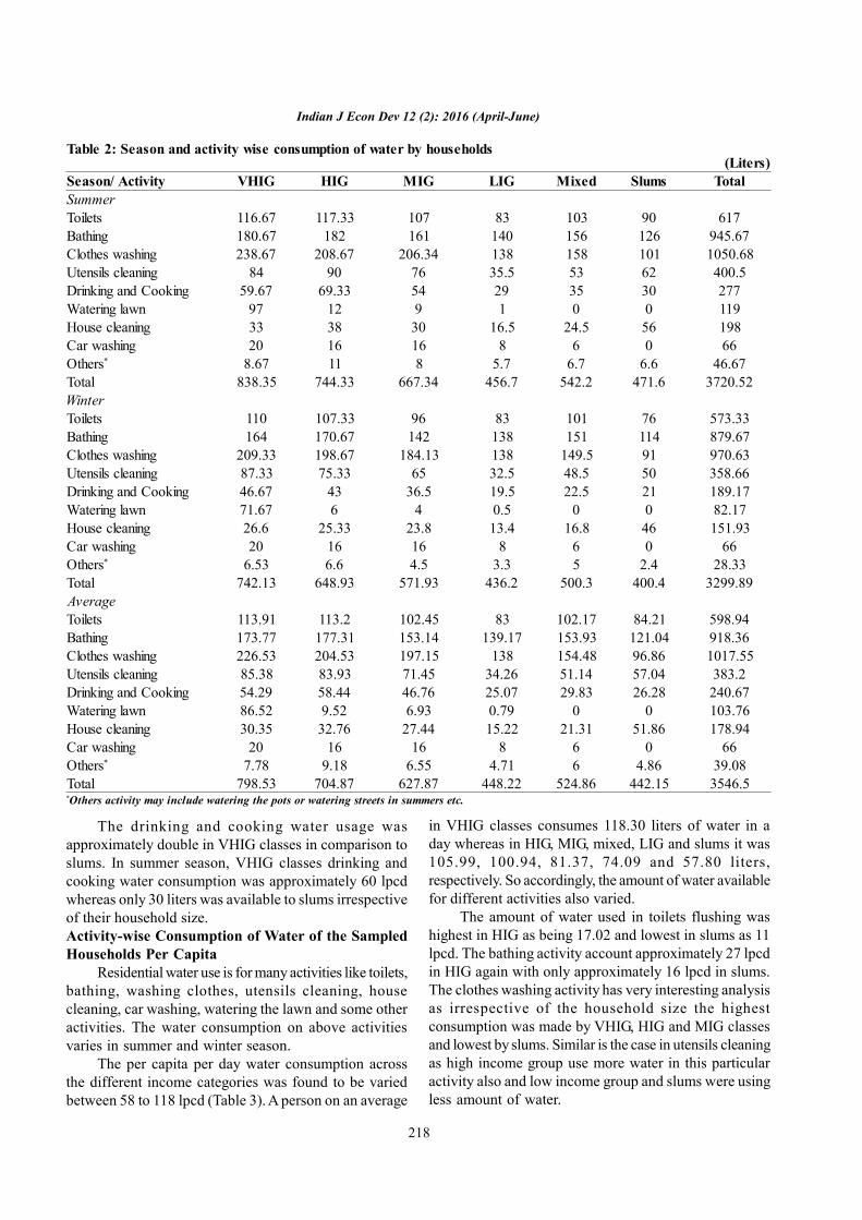
218
Indian J Econ Dev 12 (2): 2016 (April-June)
The drinking and cooking water usage wasapproximately double in VHIG classes in comparison toslums. In summer season, VHIG classes drinking andcooking water consumption was approximately 60 lpcdwhereas only 30 liters was available to slums irrespectiveof their household size.Activity-wise Consumption of Water of the SampledHouseholds Per Capita
Residential water use is for many activities like toilets,bathing, washing clothes, utensils cleaning, housecleaning, car washing, watering the lawn and some otheractivities. The water consumption on above activitiesvaries in summer and winter season.
The per capita per day water consumption acrossthe different income categories was found to be variedbetween 58 to 118 lpcd (Table 3). A person on an average
in VHIG classes consumes 118.30 liters of water in aday whereas in HIG, MIG, mixed, LIG and slums it was105.99, 100.94, 81.37, 74.09 and 57.80 liters,respectively. So accordingly, the amount of water availablefor different activities also varied.
The amount of water used in toilets flushing washighest in HIG as being 17.02 and lowest in slums as 11lpcd. The bathing activity account approximately 27 lpcdin HIG again with only approximately 16 lpcd in slums.The clothes washing activity has very interesting analysisas irrespective of the household size the highestconsumption was made by VHIG, HIG and MIG classesand lowest by slums. Similar is the case in utensils cleaningas high income group use more water in this particularactivity also and low income group and slums were usingless amount of water.
Table 2: Season and activity wise consumption of water by households(Liters)
Season/ Activity VHIG HIG MIG LIG Mixed Slums TotalSummerToilets 116.67 117.33 107 83 103 90 617Bathing 180.67 182 161 140 156 126 945.67Clothes washing 238.67 208.67 206.34 138 158 101 1050.68Utensils cleaning 84 90 76 35.5 53 62 400.5Drinking and Cooking 59.67 69.33 54 29 35 30 277Watering lawn 97 12 9 1 0 0 119House cleaning 33 38 30 16.5 24.5 56 198Car washing 20 16 16 8 6 0 66Others* 8.67 11 8 5.7 6.7 6.6 46.67Total 838.35 744.33 667.34 456.7 542.2 471.6 3720.52WinterToilets 110 107.33 96 83 101 76 573.33Bathing 164 170.67 142 138 151 114 879.67Clothes washing 209.33 198.67 184.13 138 149.5 91 970.63Utensils cleaning 87.33 75.33 65 32.5 48.5 50 358.66Drinking and Cooking 46.67 43 36.5 19.5 22.5 21 189.17Watering lawn 71.67 6 4 0.5 0 0 82.17House cleaning 26.6 25.33 23.8 13.4 16.8 46 151.93Car washing 20 16 16 8 6 0 66Others* 6.53 6.6 4.5 3.3 5 2.4 28.33Total 742.13 648.93 571.93 436.2 500.3 400.4 3299.89AverageToilets 113.91 113.2 102.45 83 102.17 84.21 598.94Bathing 173.77 177.31 153.14 139.17 153.93 121.04 918.36Clothes washing 226.53 204.53 197.15 138 154.48 96.86 1017.55Utensils cleaning 85.38 83.93 71.45 34.26 51.14 57.04 383.2Drinking and Cooking 54.29 58.44 46.76 25.07 29.83 26.28 240.67Watering lawn 86.52 9.52 6.93 0.79 0 0 103.76House cleaning 30.35 32.76 27.44 15.22 21.31 51.86 178.94Car washing 20 16 16 8 6 0 66Others* 7.78 9.18 6.55 4.71 6 4.86 39.08Total 798.53 704.87 627.87 448.22 524.86 442.15 3546.5*Others activity may include watering the pots or watering streets in summers etc.

219
Drinking and cooking activity accounts onlyapproximately 9 lpcd water in HIG and 8 lpcd each inVHIG and MIG, whereas low income categories wereable to have only 3 to 4 lpcd water for this main activity.The other activities like watering the lawn, house cleaning,car washing, watering the pots and washing the streetsetc. too show the same trend wherein high incomecategory households were able to have much water incomparison to other low income and slum households.Season-wise Consumption of Water Per Household
VHIG households consumed 838.35 liters of waterin summer and 742.13 liters in winters, thus on anaverage, 798.55 liters of water in a day. Similarly in HIG,MIG, mixed, LIG and slums the water consumption washigher in summer season than the winter consumptionof water (Table 4). In HIG, MIG, mixed, LIG and slumsthe average consumption of water per household wasapproximately 705, 628, 525, 448, and 442 liters of waterrespectively. In HIG, MIG, mixed, slums and LIG classesapproximately 744, 667, 542, 472 and 457 liters of waterwas consumed respectively in summer season. Waterconsumption in winter too shows this trend that lowincome classes and slums were having less water incomparison to other income classes.
This shows nothing but the adjustment of the peopleto the supply that they do not feel that water supplied to
them is not adequate. But this adjustment creates hygieneand sanitation problems resulting in health problems. Thedispersion statistic (S.D.) also shows wide variations inper household consumption of water in various localities.
Area and season wise per household waterconsumption is highly significant in slums and MIGclasses whereas the per household water consumptionin VHIG, HIG, LIG, and mixed are at par or equal use inboth seasons.Season-wise Per Capita Consumption of Water
The per capita water consumption gives us an ideaabout the water use by a person in various water relatedactivities. The perusal of Table 5 shows that the per capitawater consumption came to be in direct relationship withthe plot size and income class but was in inverserelationship with the household size of the household.Per capita water consumption was higher in higher incomeclasses as compared to lower income classes irrespectiveof their household size. The per capita water consumptionin summer for various income classes was higher incomparison to winter. In VHIG classes a personconsumed 124.20 liters of water per day; further for HIGit was reduced to 111.93 lpcd and for MIG, mixed, LIGand slums the water consumption per person per daycame to be 107.28, 84.06, 75.49 and 61.65 liters,
Table 3: Activity wise per capita per day consumption of water of the sampled households(Litres)
Area/ activity VHIG HIG MIG LIG Mixed SlumsToilets 16.88 17.02 16.47 13.72 15.84 11.00Bathing 25.74 26.66 24.62 23.00 23.86 15.83Clothes washing 33.56 30.76 31.70 22.81 23.95 12.66Utensils cleaning 12.65 12.62 11.49 5.66 7.93 7.46Drinking and Cooking 8.04 8.79 7.52 4.14 4.63 3.44Watering lawn 12.82 1.43 1.11 0.13 0 0House cleaning 4.50 4.93 4.41 2.52 3.30 6.78Car washing 2.96 2.41 2.57 1.32 0.93 0Others 1.15 1.37 1.05 0.79 0.93 0.63Total 118.30 105.99 100.94 74.09 81.37 57.80
Table 4: Season wise consumption of water per household (Liters per day)
Area/season
Summer Winter Average t-valueMean S.D. Mean S.D. Mean S.D.
VHIG 838.35 337.61 742.13 289.57 798.53 311.26 1.68NS
HIG 744.33 271.43 648.93 613.61 704.87 267.51 1.10NS
MIG 667.34 204.35 571.93 214.31 627.87 197.64 2.50**
LIG 456.7 221.18 436.2 209.12 448.22 212.48 0.52NS
Mixed 542.2 174.43 500.3 153.68 524.86 167.35 1.40NS
Slums 471.6 126.61 400.4 98.15 442.15 114.58 3.44***
*** and ** Significant at one and five percent level.NS: Non-significant
Kaur et al.: Domestic water consumption pattern and its linkage with socio-economic variables

220
Indian J Econ Dev 12 (2): 2016 (April-June)
respectively.If we analyze winter consumption of water, therein
also same trend was observed by different income classes.VHIG classes per capita water consumption was higherto the tune of 109.94 liters; while for HIG, MIG, mixed,LIG and slums per capita water consumption was below100 lpcd and above 50 lpcd. Similar trend was found inyearly average consumption of water. It is not that theconsumption was lower only in LIG areas and slums; incomparison to higher income classes while mixed, MIG,HIG, VHIG areas the consumption was also not adequatefrom health and sanitation aspects.
The per capita water consumption is much lowerthan what is recommended by the Bureau of IndianStandard, (IS-1172-1993) of 200 lpcd in cities havingfull flushing systems. The dispersion statistics (Standarddeviation) also shows that wide variations in per capitaconsumption of water exist within income classes. Areaand season wise per capita consumption in sampledhouseholds is insignificant i.e. per capita water use invarious income classes in summer and winter season isat par.Deficiency/Surplus in Consumption of Water on BIS-1172: 1993 Norms
The amount of water consumed by varioushouseholds in different income category households was
much lower than the Bureau of Indian Standardsrecommendations of 135 lpcd. The standardsrecommended by BIS are considered as the best standardsbecause these are based on the scientific methodology.The norms as suggested by BIS-1172: 1993, for toiletflushing was 30 lpcd but none of the household in differentincome categories was having this much of water (Table6).
There was deficiency in all the income categories ifwe see per capita per day consumption taking all theactivities together. So the deficiency in consumption ofwater showed that the water supplied to the residentswas not adequate and people try to adjust with the amountof water available to them. Similarly, in bathing, housecleaning and drinking and cooking activity also there wasdeficiency in the consumption of water in all the incomecategories. Clothes washing is the only activity on whichwater consumption was more than the norms in all theincome classes except slums. In utensils cleaning, thereis a mixed response as some were having more waterthan the norms and some were having less water.Demographic and Economic Profile vis-à-vis WaterConsumption
The field survey of the water consumption broughtout that per household and per capita water consumptionare closely linked with various socio-economic variableslike type of the household, education level, occupation
Table 6: Deficiency/surplus in consumption of water on BIS-1172: 1993 norms(lpcd)
Area/ activity Norms* VHIG HIG MIG LIG Mixed SlumsToilets 30 -13.12 -12.98 -13.53 -16.28 -14.16 -19Bathing 55 -29.26 -28.34 -30.38 -32 -31.14 -39.17Clothes washing 20 13.56 10.76 11.7 2.81 3.95 -7.34Utensils cleaning 10 2.65 2.62 1.49 -4.34 -2.07 -2.54Drinking and cooking 10 -1.96 -1.21 -2.48 -5.86 -5.37 -6.56House cleaning 10 -5.5 -5.07 -5.59 -7.48 -6.7 -3.22Total 135 -16.7 -29.01 -34.06 -60.91 -53.63 -77.2*BIS Standards: IS-1172:1993Note: Only those activities are considered for which breakup of water requirement was available in BIS-1172:1993. BIS-1172:1993 was reaffirmedin 1998, wherein for communities with a population between 20000 to 100000 - 100 to 150 lpcd and population of over 100000 - 150 to 200 lpcdwas recommended. But the breakup of 135 lpcd was given in BIS-1172: 1993 was available
Table 5: Season wise per capita consumption of water in the sampled households(lpcd)
Area/season
Summer Winter Average t-valueMean S.D. Mean S.D. Mean S.D. HH
VHIG 124.2 66.55 109.94 59.43 118.3 61.34 6.75 1.24NS
HIG 111.93 52.49 97.58 47.55 105.99 49.62 6.65 1.57NS
MIG 107.28 49.67 91.95 41.09 100.94 43.91 6.22 1.89*
LIG 75.49 43.98 72.1 35.52 74.09 37.13 6.05 0.46NS
Mixed 84.06 51.36 77.57 39.17 81.37 42.24 6.45 0.78NS
Slums 61.65 39.95 52.34 29.23 57.8 32.68 7.65 1.46NS
* Significant at ten percent level.NS: Non-significantHH: Households

221
and the income. This section describes the correlationbetween per household and per capita water consumptionwith its various socio-economic correlates.Household type and water consumption
As brought by the survey that in urban Ludhianamainly nuclear type of families are prevalent (Table 7).From the analysis of relationship between waterconsumption and household type of the surveyedhouseholds it came to light that a joint householdconsumes more water than nuclear household. The percapita water consumption of nuclear household was164.45 liters per day while for joint household it was
also varied with the occupation of the respondents. Theper household water use in case of labourer householdwas 448.82 liters per day which increased to 514.66 forself-employed, 571.11 for service class, 669.90 forbusiness households and 723.17 for the professionalhouseholds. Similarly, the per capita water consumptionwas lowest in the labourer category (60.08 liters per day)and the highest in the professional category (109.40 litersper day) as shown in Table 9. Evidently, the economicstatus of the household has a positive correlation withthe consumption of water.
Table 7: Household type and water consumption(l per day)
Household type Water use perhousehold
Householdsize
Water use percapita
Nuclear 593.68 3.61 164.45Joint 585.95 6.67 87.85
Table 8: Education level of households and water use(liters)
Education Water use perhousehold
Householdsize
Water useper capita
Illiterate 447.78 7.25 61.76Primary 486.68 7.07 68.84Above primary andbelow matric
524.64 6.65 78.89
Matric tograduation
649.02 6.45 100.62
Above graduation 657.36 6.46 101.76
87.85 liters per day.Education of head of household and water use
It was hypothesized in the study that theconsumption of water in the households is directly linkedwith the educational level of the household. The resultsof the survey confirmed this hypothesis. Per householdconsumption of water increased with the increase in thelevel of education of head of the household (Table 8).The total consumption of water of an illiterate householdwas 447.78 liters per day which increased to 657.36 litersper day in case of households having educationalqualification higher than the graduate level. In fact this isnot only because of higher level of education, it is alsobecause of higher level of income which is also closelyrelated with the level of education.
The per capita consumption of water also increasedfrom 61.76 liters per day to 101.76 liters per day as wemove from illiterate household to a household whose headwas graduate or above graduate.Occupational profile and water use
Per household and per capita consumption of water
Table 10: Household income and water use(l per day)
Income level(` lakh)
Water use perhousehold
Householdsize
Water useper capita
Upto 1 447.29 7.46 59.951-2 466.27 6.69 69.692-3 488.96 6.25 78.243-4 602.72 6.24 96.594-5 637.17 6.35 100.345-7.5 739.70 6.69 110.57Above 7.5 790.28 6.74 117.25
Table 9: Occupational profile and water use(l per day)
Occupationprofile
Water useper household
Householdsize
Water useper capita
Labour 448.82 7.47 60.08Self- employed 514.66 6.51 79.05Service 571.11 6.51 87.72Businessman 669.9 6.91 96.94Professional 723.17 6.61 109.4
Household income and water useThe analysis of data also brought out a very high
level of correlation between the level of household incomeand the consumption of water. The households havingincome up to one lac consumed 447.29 liters of waterper day with 59.95 liters per capita consumption (Table10). Per household water consumption went on increasingas we moved towards the higher income levels. The perhousehold consumption of water in the highest incomelevels (above `7.5 lakhs), was 790.28 liters per day andcorresponding per capita per day water consumption was117.25 liters. This means that the per capita waterconsumption of highest income level was almost doubleas compared to the lowest income level.
Distribution of Households According to Plot Size vis-a-vis Water Consumption
The perusal of Table 11 shows that approximately65 percent of the respondents in slums consume below
Kaur et al.: Domestic water consumption pattern and its linkage with socio-economic variables

222
Indian J Econ Dev 12 (2): 2016 (April-June)
100 lpcd of water, and approximately 40-50 percent ofrespondents of LIG and mixed houses consume this muchof little water. Around 38 and 28 percent respondents ofHIG and MIG houses consume below 100 lpcd, while avery less proportion of VHIG houses i.e. only 6.34 percentrespondents came in this range of water consumption.
A substantial number of respondents of VHIG, HIG,MIG and mixed houses consume water in the range of100-125 liters whereas LIG and slums proportion wascomparatively less in this range of water consumption.If we take above 150 liters of water consumption, thennone of the households from slums and a very lessproportion i.e. approximately 9 percent respondents ofother income classes consume this much of water, exceptVHIG, wherein around 31 percent respondents consumeabove 150 lpcd of water. The significant negativecoefficient of correlation (-0.449) indicated that theproportion of houses, where less than 100 lpcd waterwas consumed have an inverse relationship with the plotsize. Similar trend was observed in the case of waterconsumption between 100 to 125 l pcd. On the otherhand, the water consumption and proportion of houseswas in a significant positive relationship where more than150 liters of water was consumed per capita per day.CONCLUSIONS
In brief, the main source of water supply in Ludhianacity is MC/IT. The other sources of water supply maybe hand pumps or submersible pumps. The summerconsumption of water was somewhat more than thewinter. Per household and per capita consumption ofwater showed that high income groups use more waterin comparison to the low income households. The amountof water consumed in all the income classes was lessthan the norms suggested by BIS-1172:1993. It also cameto light that the consumption of water was somewhathigher in joint families in comparison to nuclear families.The education levels and water consumption patterns haspositive relationship. Similarly, the relationship betweenoccupation and household income and water consumptionwas found to be positive. As one moves up the occupationand income ladder, the consumption of water also goes
up.REFERENCESAnonymous. 1997-2002. Ninth Five Year Plan 1997-2002.
2. Planning Commission, New Delhi.Anonymous. 2002-07. Tenth Five Year Plan 2002-2007. 2.
Planning Commission, New Delhi.Anonymous. 2010. Housing condition and amenities in India.
65th Round, July 2008-June 2009. National Sample SurveyOffice. Government of India, New Delhi.
Anonymous. 2012-17. Twelfth Five Year Plan 2012-2017.2. Planning Commission, New Delhi.
Ballabh, V. 2003. Politics of water management and sustainablewater use. Indian Journal of Agricultural Economics.58 (3): 467-476.
Bedi, Jasdeep K. 2013. Domestic water consumption patternin urban Punjab: A case study of Ludhiana City. Ph. DThesis submitted to Punjabi University, Patiala.
BIS. 1993. Specifications for drinking water IS: 10500:1993.Bureau of Indian Standards, New Delhi.
Biswas, A.K. 1993. Water for sustainable development in thetwenty-first century: A global perspective. In: Biswas,Ajit K., Jellali, M., and Stout, G. (Eds.) Water forSustainable Development in the 21st Century.WaterResources Management Services, Oxford UniversityPress, New Delhi.
Kennedy, D N. 1984. Water conservation in California.Bulletin 198-84. Department of Water Resources, USA.
Marothia, K D. 2003. Enhancing sustainable management ofwater resources in agricultural sector: Role of institutions.Indian Journal of Agricultural Economics. 58 (3): 406-426.
Narayanamoorthy, A. 2003. Averting water crisis by dripmethod of irrigation: A study of two water intensivecrops. Indian Journal of Agricultural Economics. 58(3): 427-437.
National Commission on Urbanization. 1988. Report of theNational Commission on Urbanization. 1: 28. Governmentof India Press, New Delhi.
Shaban, A. and Sharma, RN. 2007. Water consumptionpatterns in domestic households in major cities.Economic and Political Weekly. 42 (23): 2190-2197.
WHO. 2003. The Right to Water, WHO, Geneva.
Table 11: Distribution of households according to plot size and water consumption(Percentage of households)
Lpcd VHIG HIG MIG LIG Mixed Slum t-valueBelow 100 6.34 37.62 28.16 46.98 45.23 64.49 -0.449***
100-125 40.39 26.63 33.84 24.21 28.25 23.78 -0.312***
125-150 22.03 25.17 28.16 20.64 17.47 11.73 -0.123***
150-200 29.56 9.14 8.47 7.15 7.89 0.00 0.363***
Above 200 1.68 1.44 1.37 1.02 1.16 0.00 0.589NS
Total 100.00 100.00 100.00 100.00 100.00 100.00*** significant at one percent level.NS: Non-significant

223
Indian Journal of Economics and DevelopmentVolume 12 No.(2): 223-228
April-June, 2016DOI: 10.5958/2322-0430.2016.00129.3
www.soed.in
Sweet Potato in Nigeria: Trends and Socio-EconomicCharacteristics of Farmers in Selected Local Government Areaof Kano StateIsah Musa Ahmad1*, Makama S.A.2 and Babagana G.A.3
1Department of Agricultural Economics, University of Agricultural Sciences, Dharwad-5800052Department of Agricultural Economics, University of Agriculrural Sciences, Raichur (Karnataka) 3Department of Crop Production, Faculty of Agriculture, University of Maiduguri, Niger, Nigeria
*Corresponding author’s email:[email protected]
Received: February 10, 2015 Accepted: March 15, 2016
ABSTRACTThe study examines the trend of sweet potato area, production and productivity and socio-economic characteristics of thefarmers in Gaya zone, Kano State, Nigeria. A sample of 120 farmers was randomly selected from three LGAs of the state.Primary data were collected through the use of structured questionnaire and were analyzed using descriptive statistics.Secondary data on area, production and productivity were obtained from FAOSTAT. Results of the analysis revealed that,area harvested increased from 28,000 Ha in 1990 to 933,500 ha in 2010, and production increased tenfold over the last20 years while yields showed a notable decline over the same period (from 5.1 metric tonne per ha in 1990 to 2.9 metrictonne per ha in 2011). Results further revealed that majority (43.3 percent) of the respondents were within the age of 30-42 years with mean age of 34 years, 70.83 per cent were males and majority (51.67 percent) attended non formaleducation, 45 per cent had farm size of between 0.2 -1.0 ha, and majority (85.83 percent) inherited their farm land.Majority of the respondents (85.8 percent) have experience of between 1-15 years. Findings also revealed that, poorprice, poor access to markets and credits, were the major constraints faced by farmers in the study area. The studytherefore suggested that, extension services should be enhanced and farmers are advice to form co-operative groups toenable them pool their resources and ease their credit needs. Government on the other side should ensure timely supplyof agricultural credits at low rate as well as provision roads that will link farming communities to the markets.
KeywordsFarmers, production, socio-economic characteristics, sweet potato, trend
JEL CodesD24, J01, J10, O13
INTRODUCTIONNigeria is the third largest producer of sweet
potatoes in the world in terms of quantity, after Chinaand Uganda. In 2010, Nigeria produced 2.5 percent ofthe world’s production of sweet potatoes. However,sweet potatoes are still considered as minor crop in thecountry. Sweet potatoes had the tenth highest productionlevel of any single food crop in Nigeria (after cassava,yam, oil palm fruit, maize, sorghum, millet, paddy rice,and plantains) in 2001. The gross agricultural productionvalue for sweet potatoes in the year 2010 was $954million and accounted for 1.73 percent of total
agricultural production value for all crops (Walker et al.,2011).
Currently, Sweet potato is an important crop in manyareas of the world being cultivated in over 100 countries.It ranks among the five most important food crops in thetropical areas where a high population of the world’spoorest people live. However, it ranks fourth in terms ofworld most important food crops, after rice, wheat, andcorn (Babatunde et al., 2007 and Jude, 2011).
In Nigeria, sweet potato cultivation is still restrictedto a few states and its production is mainly for localconsumption. Tewe et al. (2003) indicated that, Sweet

224
Indian J Econ Dev 12 (2): 2016 (April-June)
potato (Ipomoea batatas) is only a minor root crop intropical Africa despite its potentials as indicated by itsgrowth in terms of production. Among the root and tubercrops, it is the only one that had positive per capita annualrate of increase in production in sub-Saharan Africa. Sweetpotato received less intervention in the country as regardto boosting its production and utilization, but still it hashigher growth rate than other root crops like yam andcassava. Anonymous (2007) revealed that potatoproduction grew by 7.3 percent in 2007 compared to 5.5percent in 2006. However, yield estimate of sweet potatoin Nigeria vary widely among different agro-ecologicalzones.
Sweet potatoes have a number of additionalagricultural and industrial uses as well. Sweet potatovines, leaves and roots are used for animal feed for sheep,goats, and rabbits (Abu, 2003). Recent studies found thatanimals that are fed sweet potato vines actually produceless methane gas than animals given other types of feed,suggesting that sweet potato animal feed can help inreducing global emissions (International potato center).Sweet potatoes are also processed industrially into friedsnacks like sweet potato fries (chips), candy, starch,noodles, and flour. There is high demand in urban areasfor fried sweet potato crisps (Akoroda, 2009). Sweetpotatoes can also be exploited for ethanol and biofuelproduction. Sweet potatoes can be processed to yieldabout 137 liters of ethanol per MT of sweet potato tubers(Akoroda, 2009). Worldwide, sweet potato’s productionand consumption is huge. All over the world people eatand use this super food. In Nigerian the demands is quitehigher than the supply (Ajakaiye et al., 1999). The feedingof over 160 Million Nigerians is a common task but mustbe accomplished; otherwise poverty, malnutrition andhunger will increase rapidly in the coming years (Adegbolaand Olayemi, 1997).
Little research is known to have been undertakenon the economics of sweet potato production comparedto other roots and tubers like cassava, and yam. (Akinwumi2002). This study therefore, is important as a tool forNigeria to achieve the millennium development goalswhich are targeted towards poverty reduction and hunger,combating diseases and epidemics and finally developinga global partnership for development.Objectives of the Study
The study was focused toward achieving thefollowing objectives:i. to describe the trend of area, production and
productivity of sweet potato in Nigeria from 1990-2012,
ii. to describe the socio-economic characteristics ofsweet potato farmers in the study area, and
iii. to examine the constraints limiting sweet potato
production in the study area.MATERIALSAND METHODSStudy Area
Kano State is located on latitude 13.53 N and 10.25Nand longitude 7.4E and 10.53E. It shares boundary withJigawa State to the North East, Katsina State to the NorthWest and Kaduna State to the South. The State isadministratively divided into 44 local government areas.According to Anonymous (2006), the state has apopulation of 9.4 million with 446 person/km2 density.The estimated population as at 2008 and 2009 was be9.88 and 10.11million respectively at 2.5 per cent annualincrease. The annual rainfall of the state range between420mm 1000m and temperature is averagely warmthroughout at about 270c + 70c (Anonymous, 2007).Data Collection
Purposive random sampling technique was usedto select three 3 Local Government Areas that producessignificant quantities of Sweet potatoes within Gayaagricultural zone in the state. Albasu, Sumaila and Garkolocal government areas were purposively selected as such.Likewise, two villages with high sweet potato productionwere selected in Albasu and Sumaila, while three fromGarko respectively. From these Villages, three identifiedsweet potato farmer groups were randomly selected fromAlbasu and Garko, while two farmer groups in Sumailawere identified respectively. Moreover, 15 farmers wererandomly selected in each of the identified farmer groupsrespectively making the sum of 120 respondents.Analytical Techniques
The data were analyzed using descriptive statisticssuch as percentages, frequency tables and means.RESULTSAND DISCUSSION
In 2010, sweet potatoes had the tenth highestproduction level of any single food crops in Nigeria (aftercassava, yam, oil palm fruit, maize, sorghum, millet, paddyrice, and plantains). The gross agricultural productionvalue for sweet potatoes in 2010 was $954 million andaccounted for 1.73 per cent of total agricultural productionvalue for all crops (Walker et al., 2011).
The data suggest that sweet potato production hasincreased tenfold over the last 20 years, although someobservers suggest that the data reflect the state of disarrayof Nigeria’s agricultural statistics rather than actual growthin production. FAOSTAT data show that area harvestedhas increased rapidly through the past 20 years though ithas been somewhat in decline since 2007; in addition,production expanded greatly until 2006, after whichproduction has also been quite erratic (Table 1).
Sweet potato production continues to reflectsignificant yield gaps and stagnant productivity. Whilethe area harvested increased from 28,000 ha in 1990 to

225
Ahmad et al.: Sweet sotato in Nigeria: Trends and socio-economic characteristics of farmers
933,500 ha in 2010, yields have shown a notable declineover that same period (Table 1). The yield for sweetpotatoes was 2.9 MT/ha in 2011, down from 5.1 MT/hain 1990. In the 1960s, sweet potato yields were as highas 12.4 MT/ha.
The negative association between area harvested andyield is common to sweet potato data in Sub-SaharanAfrica, not just Nigeria. Walker et al. (2011) indicate thatone explanation is that sweet potatoes were planted onmore marginal land. It was believed it is more likely thatdecision makers releasing sweet potato statisticsmanipulated the yield downward (without any empiricalevidence). In addition, the declining productivity can beattributed to the non-adoption of modern farming practiceslack of improved varieties, none or low application ofinorganic fertilizer.Socio-economic Characteristics
In Nigeria, the possibilities for agriculturalimprovement are influenced by some socio-economic,political and as to some extent the prevailing environmentalas well as by some technical factors (Garba, 2008). It isevident from the Table 2 that majority of the respondents(70.83 percent) are males, while only 29.16 per cent ofthem are females. Thus, it can be said that majority of the
Table 2: Distribution of respondents according socio-economic characteristicsVariable Frequency PercentageGenderFemale 35 29.16Male 85 70.83Age (Years)17 - 29 40 33.3330 - 42 52 43.3343 - 55 19 15.8356 and Above 09 7.50Mean 34.5 100.00Farming experience (Years)01 - 15 103 85.8316 - 30 12 10.0031 - 45 01 0.83> 46 05 4.16Mean 15 yearsEducational levelNon formal 62 51.67Adult 20 16.67Primary 18 15.00Secondary 12 10.00Post secondary 08 06.67Source: Field Survey, 2012
Table 1: Area harvested and production of sweet potatoes in Nigeria, 1990-2012Year Area Harvested ('000 Ha) Production ('000MT) Productivity (Kg/ha)1990 140,000 715,000 25535.71991 155,000 920,000 29677.41992 255,000 1,090,000 21372.61993 345,000 1,795,000 26014.51994 345,000 1,525,000 22101.51995 1,495,000 5,840,000 19531.81996 1,505,000 7,390,000 24551.51997 1,665,000 7,465,000 22417.41998 1,411,000 7,800,000 27639.91999 4,085,000 12,255,000 15000.02000 4,115,000 12,340,000 14993.92001 4,120,000 12,365,000 15006.12002 4,385,000 13,155,000 15000.02003 4,475,000 14,000,000 15642.52004 4,770,000 14,980,000 15702.32005 4,945,000 16,025,000 16203.22006 5,105,000 17,310,000 16953.92007 5,655,000 12,160,000 10751.62008 5,530,000 16,590,000 15000.02009 5,500,000 16,500,000 15000.02010 5,500,000 16,500,000 15000.02011 5,500,000 16,500,000 15000.02012 5,575,000 17,000,000 15246.6Source: FAOSTAT

226
Indian J Econ Dev 12 (2): 2016 (April-June)
Sweet Potato farmers sampled in the study area are malesas the prevailing norm of the region. The results indicatesthe age category 30-42 years forms the majority of therespondents which are young and perhaps active withinthe economically productive age as defined by FAO, 2003(15-64 years); while none of the respondents fall belowthe age of 15 or above 70 years which is the dependentage as stipulated by FAO, 2003.
Further, the overwhelming majority of the farmershave farming experience between 1-15 years and thisagrees with the findings of Garba et al. (2008), that Sweetpotato farming experience is 1-10 years. About 56 percent of respondents possess only non-formal education,conversely Tewe et al. (2003) expressed that, twentypercent (20 percent) of the respondents were educatedup to first school leaving certificate.Access to Productive Resources
The findings also disclosed that large proportion ofthe respondents 45 per cent cultivate farm size less orequal to one hectare (Table 3). The average farm size is1.13 hectares, which suggest that majority of the farmersin the study area are small scale farmers. Contrary to thestudy of Garba et al. (2008), who reported in a surveyconducted in Toro (Bauchi State) showing that 51.7 per
cent of the farmers cultivate between 1-2 ha of land. Onthe other hand, the result showed that 85 per cent of theland cultivated by respondents was owned throughinheritance and more than 50 per cent of respondentsuse family labour as the main source of labour and 73.3per cent uses fertilizer in sweet potato farms. However,Jude et al. (2011) reported that an average sweet potatofarmer used 46.30kg of fertilizer. On the other hand,Gbigbi (2011) stressed that, on average 650.36 kg ofseed, and 105.24kg of fertilizer were used by farmers.Moreover, the study reveals that, 76 percent of therespondent’s source of capital is personal savings, 13.33from friends and relatives and 10 percent from Banks.This implies that farmers in the study area have verylimited contact with financial institutions and needs to belinked more to financial institutions to enable farmersobtain credit/loans and other financial benefits.Constraints to Sweet Potato Farming in the StudyArea
The results presented in Table 4 revealed that poorprices (75 percent), poor access to market (59.2 percent)and poor access to credit (48.3 percent) were the seriousproblems limiting sweet potato production in the studyarea. Ellen et al. (1994) noted that, the major constraint
Table 3: Distribution of respondents according to access to productive resourcesVariable Frequency PercentageFarm size (ha)0.2 - 1.0 54 45.01.1 - 1.9 21 17.52.0 - 2.8 16 13.332.9 - 3.7 08 6.663.8 and above 21 17.5Land ownershipInheritance 103 85.83Purchase 13 10.83Borrowed 02 1.66Rent/Lease/Hired 02 1.66Source of labourFamily 61 50.83Communal 55 45. 83Hired 04 4.17Source of capitalPersonal saving 92 76.66Friends and relatives 16 13.33Banks 12 10.00Use of fertilizer (kg)None 16 26.7025-100 34 56.70101200 08 13.30201-300 02 3.30Source: Field Survey, 2012

227
REFERENCESAbu, I. A. 2003. Economics of production and postharvest
technology in food yams In: Advances in research.Okwor, G.C, Asiedu, R.A, Ekanayake, I.J (eds.). NRCRIUmudike/IITA, Ibadan, Nigeria:187- 214.
Adegbola, P.S. and Olayemi, J.K.1997. The influence ofeducation and extension contact on food cropproduction in Gombe state, Nigeria. Journal ofAgribusiness and Rural Development. 1 (1): 80-92.
Ajakaiye D.O. and Akande, S.O. 1999. National AgriculturalResearch Programme in Nigeria. A characteristic ofindustrial demand for agricultural commodities inNigeria, NISER, Ibadan: 4-5.
Akinwumi, M.O. and Adebayo, F.A. 2002. Profitability andtechnical efficiency of sweet potato production inNigeria. Journal of Rural development. 31 (5): 105-120.
Akoroda, M. 2009. Sweet potato in West Africa. In: G.Loebenstein, G. and ThottapPilly, G. (Eds.). TheSweetpotato. Springer, Netherlands: 441-468.
Anonymous. 2006. National Population Commission 2006Nigerian Provisional population Figures. No. 1, MasakaClose Off Olusegun Obasanjo Way, Wuse Zone 7, Abuja,Nigeria.
Anonymous. 2007. Central Bank of Nigeria annual report andstatement of accounts, December: Federal CapitalTerritory, Abuja, Nigeria: 1-241.
Anonymous. 2007. Kano State Agricultural and RuralDevelopment Authority. Annual Report, 2007 Kano,Nigeria.
Babatunde, R. O., Olorunsanya, E. O., Orebiyi, J. S. and Falola,A. 2007. Optimal farm plan in sweet potato croppingsystems: A case of Offa and Oyun local governmentareas of Kwara State, North- Central, Nigeria.Agricultural Journal. 2 (2): 285-289.
Bamire, A. S.; Oluwasola, O. and Adesiyan, A. T. 2007. Landuse and socio-economic determinants of technicalefficiency of rice farms in Osun state, Nigeria. In: Haruna,U., Jibril, S.A., Mancha, Y.P., and Nasiru, M. (eds).Consolidation of growth and development of agriculturalsector. In: 9th Annual National Conference of theNigerian Association of Agricultural Economists.Abubakar Tafawa Balewa University Bauchi, Nigeria:27-35
Ellen, P., Gregory, B.K. and John, W.S. 1994. Study of womenin agricultural marketing in Chad. AMIT Project(Agricultural Marketing, and Technology Transfer)Funded By United States Agency for InternationalDevelopment USAID Ndjamena, Chad. PublicationAMIT No.53: 40-53.
FAO. 2003. Food and Agricultural Organisation of the UnitedNations. Production year book. FAO Rome. 40: 307.
Garba, M. 2008. Economics of sweet potato production inToro L.G.A. An undergraduate project submitted toAgricultural Economics and Extension ProgrammeATBU, Bauchi, Nigeria.
Ahmad et al.: Sweet sotato in Nigeria: Trends and socio-economic characteristics of farmers
preventing farmers from mobilization of funds appearsto be the lack of any sort of secured deposit facility. Therespondents also faced the problem Pest and Disease,modern storage and processing technology, implying thatmost sweet potato farmers in the study area relied onlocal storage and processing facilities.
However, Tewe et al. (2003) noted that constraintsin the industrialization of sweet potato in Nigeria includelack of storage technology and processing equipment,unavailability of farms inputs, marketing problems, andinadequate improved varieties among others. The resultalso indicated that, sweet potato farmers reported poorextension service and high cost of inputs as one of theproblem limiting their production. This is similar withBamire et al. (2007) who observed that, 84.30 per centof farmers reported problem of high cost of inputs inOsun State.CONCLUSIONAND RECOMMENDATIONS
This study was conducted to examine the trend ofarea, production and productivity in Nigeria and socio-economic factors of sweet potato farmers in Albasu,Garko and Sumaila LGA of Kano State. However, theresults of the study indicated that males represent 70.83per cent of sweet potato farmers in the study area. Thisshowed that the enterprise is gender bias. However, thereis the need to create awareness especially on the womenpart. In addition, effort should be made to minimize theconstraints faced by the farmers in the study area suchas making credit facilities accessible and affordable tothe farmers, strengthening extension service programs,formation of farmer groups or co-operatives to handlethe case of supplying farm inputs and marketing of theirproducts collectively among others. The study furtherrecommended that high yielding varieties should bedeveloped and made accessible to farmers so as to boostsweet potato enterprise in the study area. Similarly, agro-processing industries should be established to enhancesweet potato processing and utilization in order to reducepoverty and achieve food security.
Table 4: Distribution of respondents according toconstraintsConstraints Frequency PercentagePoor price 90 75.0Poor access to market 71 59.2Poor access to credit 58 48.3Pest and disease 36 30.0Insecurity 34 28.3Poor extension service 32 26.6High cost of input 31 25.8Inadequate infrastructure 23 19.2Source: Field Survey, 2012
228
Indian J Econ Dev 12 (2): 2016 (April-June)
Gbigbi, M. T. 2011. Economic efficiency of smallholder sweetpotato producers in Delta State, Nigeria. ResearchJournal of Agriculture and Biological Sciences. 7 (2):163-168.
Jude C.N., Benjamin, C.O., and Patrick, C.N. 2011. Measurementand determinants of production efficiency among small-holder sweet potato ( Ipomoea batatas ) farmers in ImoState. European Journal of Scientific Research. 59 (3):307-317.
Tewe, O.O., Oyeniyi F. F., and Abu O. A. 2003. Sweet potatoproduction, utilization and marketing in Nigeria.International Potato Centre (CIP) Lima, Peru.
Walker, T., Thiele, G., Suarez, V., and Crissman, C. 2011.Hindsight and foresight about Sweet potatoproduction and consumption. International PotatoCenter, Lima, Peru.
Webliographyhttp://www.fao.org/home/en/

229
www.soed.in
Socio-economic Impact of Enterprises Adoption on Self-helpGroup Households in PunjabNirbhai Singh*, Sanjay Kumar, and Jasdev Singh1
1Department of Economics and Sociology, Punjab Agricultural University, Ludhiana-141004
*Corresponding author’s email: [email protected]
Received: November 24, 2015 Accepted: May 16, 2016
Indian Journal of Economics and DevelopmentVolume 12 No. 2: 229-236
April-June, 0000DOI: 10.5958/2322-0430.2016.00130.X
ABSTRACTThe socio-economic impact of adoption of the enterprises on SHG member households has been studied in the Punjabstate by selecting the districts of Ludhiana, Jalandhar and Hoshiarpur. A sample of 30 SHGs was selected randomly fromthese districts. Amongst the selected SHGs, 2 members from each of the SHG were randomly selected making a total sampleof 60 respondents. Amongst the activities, the sample SHG members were found to adopt pickle and murabba, bee-keeping, papad/baddi and candle making enterprise, which were finally selected for the detailed analysis. The referenceyear of the study was 2014. The results of the study showed that SHGs had good impact on saving, income, assetsformation, employment and other social aspects of the members. The SHG member households confronted the problemsduring opening of bank account, low credit delivery, high rate of interest on credit amount, lack of training, marketingproblems and competition from MNCs. But it requires a lot more efforts on part of the government as well as the bankingsector to promote SHGs in the state. There is need to focus on awareness programmes for adopted economic activities,training facilities and providing credit delivery.
KeywordsSelf Help Groups, socio-economic impact, problems and prospects.
JEL CodesC81, C82, G21, Q13
INTRODUCTIONIndia, being a developing nation, has approximately
22 percent of its total population of 1.21 billion below thepoverty line (Anonymous, 2011). Provision of servicesto the poor and underprivileged sections of the societyhas always been in focus of various programmes initiatedby the government since independence (Dasgupta, 2001).However, anti-poverty or welfare measures, launched bythe government often tend to miss the targeted population.These poor people have skill, labour, zeal to work butthey lack capital. Therefore, credit plays an importantrole in rural development and poverty alleviation (Dattaand Raman, 2001). The structure of the rural financialmarket in India is dualistic consisting of both formal andinformal financial intermediaries. Since independence, theformal banking institutions had ignored the poor due toperceived high risks, high transaction costs involved insmall-scale rural lending to a large number of poorhouseholds and absence of collateral securities. In theabsence of a healthy institution- customer relationship
and the resulting unsatisfactory institutional supply ofcredit, the informal financial system continued to fulfilthe needs of the credit. Against this backdrop of failures,microfinance schemes using self-help groups (SHGs)were designed (Mansuri, 2010). Self-help group hasevolved as an accepted institutional framework to providefinancial services to the poor. Further, it is regarded asbetter mechanism to reduce poverty gradually as againstgiving one time loan for productive assets which may ormay not lead to sustained increase in income(Madheswaran and Dharmadhikary, 2001).
Many studies have made an attempt to study thesocio-economic impact of enterprises adopted bydifferent self-help groups in India. Manimekalai andRajeswari (2000) found that the income of the womenself-help groups formed by a sample NGO inTiruchirapalli, Tamil Naidu had improved from a meanincome of `4800 to `50874 after owing a micro enterprisethus providing them economic and social empowerment.Puhazhendhi and Satyasai (2001) studied the impact of

230
Indian J Econ Dev 12 (2): 2016 (April-June)
formation of self-help groups in 11 states of the country.The study revealed that 59 per cent of the samplehouseholds registered an increase in assets. The studyfurther revealed that 33 per cent increase in net incomefrom `20177 per household in the pre-SHG situation and47.9 percent of the families moved above the povertyline after formation of SHGs. Social empowerment wasalso evident in post SHG situation as measured byimprovement in their confidence, their treatment withinthe family, communication skill and other behaviouralchanges. Banerjee (2002) in his study on self-help groupsin four districts of Tamil Naidu found that saving doubledto `1216 per year per member as compared to presituation. The repayment was almost 100 per cent.
Moreover, the annual employment available to groupmembers increased by 85 per cent i.e. 172 man days inpost situation by undertaking supplementary activitiessuch as animal husbandry, poultry and non-farm activitieslike petty shops, kirana shops, etc. Singh (2006)conducted a study in Punjab state and found that afterjoining the SHG, the average annual income of memberhouseholds increased to ‘ 54474 showing about 76 percent increase than pre SHG situation. Further, majorityof the members (85 per cent) agreed that their influenceon economic resources of the family had increased afterjoining SHGs. Sorokhaibam (2014) conducted a study inPunjab and found that after joining the SHGs, averageannual income of the members increase to `82960showing about 29 percent increase from the pre-SHGsituation. Majority of the members revealed that theirinfluence on economic resources, decision making abilityand the status of their family in the society had increasedafter joining the groups.
The present study was therefore, designed to studythe socio-economic impact of enterprises adopted bydifferent SHG member households in Punjab.METHODOLOGY
Three districts having the highest number of SHGsin Punjab were selected namely, Ludhiana, Jalandhar andHoshiarpur. A detailed list of SHGs who have started theeconomic activities in these districts was obtained fromthe NABARD office and DRDA office. A sample of 30SHGs was selected randomly from these districts.Amongst the selected SHGs, 2 members from each ofthe SHG were randomly selected making a total sampleof 60 respondents. The main activities undertaken by SHG
member households in Punjab includes dairy, tailoring,pickle and murabba, football making, bee-keeping, banmaking, candle making, papad/baddi, surf making etc.(Singh, 2006 and Sorokhaibam, 2014). Amongst theseactivities, the selected sample SHG members were foundto adopt pickle and murabba, bee-keeping, papad/baddiand candle making enterprises, which were finally selectedfor the detailed analysis. The detail of enterprise wisenumber of selected SHGs and member households isprovided in Table 1.
Data were collected personally with the help ofstructured and pre-tested interview schedule developedfor the study. Presidents of the SHGs were identified andwith the help of presidents other members of the groupswere identified. Both primary and secondary data wereutilized in the present study.RESULTSAND DISCUSSIONSocio-economic Characteristics of the MemberHouseholds of the SHGs
About half of SHG member households werebetween the age group of 40-50 years. The average ageof SHG member households was found to be 41 years.About 28 percent of the sample member households wereilliterate. Of the literates, about 30 percent had studied upto primary followed by middle (about 20 percent), highschool (about 13 percent), graduation and above (about5 percent) and higher secondary (about 3 percent). About70 percent of the sample member households were livingin nuclear family. Most of the member households (about67 percent) had family members in the range of 5-7persons and the average family size was observed to be6 members per family. Most of the member households(about 38 percent) were belonging to the SC category.About 83 percent of the houses of the member householdswere pucca in nature and remaining 17 percent were semipucca. Most of the member households (about 38 percent)were involved in business followed by farming (about 35percent), labour (about 18 percent) and service (about 9percent) in Table 2.Socio-economic Impact of Adoption of the Enterpriseson SHG Member Households1. Impact of SHGs on the economic aspects of theSHG member households
An attempt has been made in this section tounderstand the economic benefits accrued to the membersdue to their involvement with the self-help groups based
Table 1: Classification of the sample SHG member households according to their adopted enterprisesParticulars Enterprises
Pickle and Murabba Bee-keeping Papad/baddi Candle making OverallNumber Percent Number Percent Number Percent Number Percent Number Percent
SHGs 12 40.00 6 20.00 6 20.00 6 20.00 30 100.00Respondents 24 40.00 12 20.00 12 20.00 12 20.00 60 100.00

231
Singh et al.: Socio-economic impact of enterprises adoption on self help group households in Punjab
Table 2: Socio-economic characteristics of the members of the SHGs, Punjab, 2014Particulars Enterprises
Pickle and murabba Bee-keeping Papad/baddi Candle making OverallNumber Percent Number Percent Number Percent Number Percent Number Percent
Age (years)20-30 2 8.33 ÑÑ 1 8.33 1 8.33 4 6.6730-40 8 33.33 5 41.67 7 58.33 4 33.34 24 40.0040-50 13 54.17 6 50.00 2 16.67 6 50.00 27 45.0050-60 1 4.17 1 8.33 2 16.67 1 8.33 5 8.33Average age(Years)
41 44 39 42 41
EducationIlliterate 7 29.17 1 8.33 2 16.67 7 58.33 17 28.34Primary 7 29.17 4 33.34 5 41.66 2 16.67 18 30.00Middle 5 20.83 3 25.00 2 16.67 2 16.67 12 20.00High school 2 8.33 2 16.67 3 25.00 1 8.33 8 13.33Higher secondary 1 4.17 1 8.33 ÑÑ ÑÑ 2 3.33Graduation andabove
2 8.33 1 8.33 ÑÑ ÑÑ 3 5.00
Family typeNuclear 15 62.50 8 66.67 10 83.33 9 75.00 42 70.00Joint 9 37.50 4 33.33 2 16.67 3 25.00 18 30.00Family size (No.)1 to 4 6 25.00 2 16.67 4 33.34 2 16.67 14 23.335 to 7 16 66.67 8 66.66 7 58.33 9 75.00 40 66.67>7 2 8.33 2 16.67 1 8.33 1 8.33 6 10.00Average size(No.)
5.67 6.08 5.33 5.75 5.70
Social classGeneral 6 25.00 5 41.67 8 66.66 2 16.67 21 35.00SC 11 45.83 3 25.00 2 16.67 7 58.33 23 38.33OBC 7 29.17 4 33.33 2 16.67 3 25.00 16 26.67House 50Pucca 19 79.17 12 100.00 11 91.67 8 66.67 50 83.33Semi-pucca 5 20.83 1 8.33 4 33.33 10 16.67Main OccupationService 2 8.33 2 16.67 1 8.33 5 8.34Farming 14 58.34 6 50.00 1 8.33 21 35.00Business 3 12.50 4 33.33 9 75.01 7 58.33 23 38.33 Labour 5 20.83 1 8.33 5 41.67 11 18.33Figures in the parentheses indicate per cent to the total.
on thrift and credit and start of the economic activities.Economic empowerment is the initial aspect ofdevelopment and it means greater access to financialresources, reducing helplessness of poor to crisissituations and development of entrepreneurship amongthe member households. Major economic indicators likeincome, saving, borrowings, occupation and assets werestudied in this section. The impact was ascertainedthrough the quantitative change in these parameters inpre and post SHG situation and presented in the followingsub sections:
Impact on the Level and Composition of HouseholdIncome
Based on the responses of the SHG members underthe study, data regarding the average annual income ofthe family before and after involving in SHGs weregathered and summarized in Table 3 and 4. From theTable 3 it can be seen that before involving in SHGs,most of the member households (about 48 percent) earnedan average of `50000-`100000 per annum and 25 percentof the member households had average annual income

232
Indian J Econ Dev 12 (2): 2016 (April-June)
between `100000-`150000 and only 3 percent of themember household earned more than `250000. However,after being involved in the SHGs, the average annualincome of the majority of the respondents (about 25percent) was between `100000-`150000. The percentageof households who earned between `50000-`100000decreased from 48 to 22 percent and those who earnmore than `250000 per annum increased from about 3to 18 percent.
The perusal of Table 4 revealed that the share ofincome in household income of member households fromservice, farming and labour decreased in post SHGsituation. But in absolute terms, their average annualincome from service increased to `23000 in post SHGsituation from `20667 in pre SHG situation, to `51167 inpost SHG situation from `44333 in pre SHG situationfrom farming and to `15617 from `13283 in case of
labour. The share of business activity in total householdincome increased from about 40 percent in pre-SHGsituation to about 55 percent in post-SHG situation. Afterjoining the SHGs, the total average annual householdincome of the members increased to `199650 a jump ofabout 50 percent as compared to the pre-SHG situation.Impact on Savings of the Member Households
Table 5 presents the average annual savings of themember households in pre and post-SHG situation. Itmay be noted that about 82 percent of the sample memberhouseholds were savings in pre-SHG situation ascompared to almost all the members saving in post-SHGsituation. Majority of the households, (about 33 percent)were saving up to `2500 in pre-SHG situation whichdecreased to about 22 percent in post-SHG situation. Afterjoining the SHG, some member households had moresaving and they were included in next category that is
Table 3: Distribution of sample member households according to the annual household income, Punjab, 2014(Percent)
Income level(`)
Enterprises OverallPickle and murabba Bee-keeping Papad/baddi Candle making
Pre-SHG50000-100000 54.17 16.67 41.67 75 48.33100000-150000 20.83 25 33.33 25 25150000-200000 12.5 33.33 25 16.67200000-250000 8.33 16.67 6.67>250000 4.17 8.33 3.33Total income (`) 126667 177917 124167 95167 130117Post-SHG50000-100000 29.17 8.33 41.67 21.67100000-150000 33.33 25 33.33 25150000-200000 20.83 41.67 25 21.67200000-250000 12.5 16.67 25 13.33>250000 4.17 83.33 18.33Total income (`) 165625 402500 154333 110167 199650
Table 4: Source-wise composition of annual household income for sample member households, Punjab, 2014(` per member household)
Source ofincome
EnterprisesPickle and murabba Bee-keeping Papad/baddi Candle making OverallAmount Percent Amount Percent Amount Percent Amount Percent Amount Percent
Pre-SHGService 21250 16.78 45833 27.76 15000 12.08 - - 20667 15.88Farming 70000 55.26 65000 36.53 16667 13.42 - - 44333 34.07Business 20417 16.12 67083 37.70 85833 69.13 65417 68.74 51833 39.84Labour 15000 11.84 6667 5.37 29750 31.26 13283 10.21Total 126667 100.00 177917 100.00 124167 100.00 95167 100.00 130117 100.00Post-SHGService 24167 14.59 47500 11.80 19167 12.42 - - 23000 11.52Farming 81250 49.06 72500 18.01 20833 13.50 - - 51167 25.63Business 42083 25.41 282500 70.19 106000 68.68 76667 69.59 109867 55.03Labour 18125 10.94 8333 5.40 33500 30.41 15617 7.82Total 165625 100.00 402500 100.00 154333 100.00 110167 100.00 199650 100.00

233
Singh et al.: Socio-economic impact of enterprises adoption on self help group households in Punjab
Table 5: Distribution of sample member households according to the average annual saving, Punjab, 2014(`)
Saving EnterprisesPickle and murabba Bee-keeping Papad/baddi Candle making OverallAmount Percent Amount Percent Amount Percent Amount Percent Amount Percent
Pre-SHGUp to 2500 1725 33.33 2333 25.00 1640 41.67 1550 33.33 1760 33.332500-5000 3417 25.00 3300 16.67 3800 16.67 3500 16.67 3475 20.005000-7500 6000 16.67 6167 25.00 6250 16.67 5500 8.33 6050 16.677500-10000 8250 8.33 8250 16.67 8000 8.33 8000 8.33 8167 10.00>10000 - - 24000 8.33 - - - - 24000 1.67Average 3117 83.33 6050 91.67 3025 83.33 2225 66.67 3507 81.67Post-SHGUp to 2500 2340 20.83 2500 8.33 2333 25.00 2250 33.33 2323 21.672500-5000 4113 33.33 4900 16.67 4500 33.34 4867 25.00 4429 28.335000-7500 6643 29.17 7250 16.67 7167 25.00 7250 16.67 6929 23.337500-10000 8900 12.50 9733 25.00 9000 8.33 8000 16.67 8838 15.00>10000 18000 4.17 33000 33.33 11000 8.33 10500 8.33 16125 11.67Average 5658 100.0 15667 100.00 5542 100.00 5383 100.00 6582 100.00
about 20 per cent member households were savingbetween `2500-`5000 in pre-SHG situation whichincreased to about 28 percent in post-SHG situation.Therefore, about 17 percent member households weresaving between `5000-`7500 in pre-SHG situation whichincreased to 23 percent in post-SHG situation. About 2per cent member households were saving more than`10000 in pre-SHG situation but in post-SHG situationthe proportion of these member households increased toabout 12 percent. The average annual saving of the samplehouseholds in pre-SHG situation was `3507 whichincreased to `6582 after joining the SHGs.Impact on Asset Position
The household assets consist of houses, farmhouses, animal sheds, milch and working animals,productive assets such as tractor, farm equipments,cartload, auto rikshaw, taxi, tools, etc. and consumer
durables consists of television, refrigerator, vehicles andsome other household durables. However, the impact wasexamined through the change in animal assets, productiveassets and consumer durables in pre and post-SHGsituation.
Table 6 presents detailed analysis of the assetsposition of the sample member households. About 43 percent increase in the overall average value of assets canbe seen from `118731 in pre-SHG situation to `170345in post-SHG situation. The increase in assets of the samplehousehold may be due to the increase in their purchasingpower as a result of easy access to credit facility throughSHG. The average value of productive assets had a majorshare to the total average value of assets both in pre-SHG (48.85 percent) and post-SHG (49.29 percent)situation. The share of animal assets decreased to about26.42 percent in post-SHG situation from 29.17 percent
Table 6: Asset position of the sample member households, Punjab, 2014(`)
Assets EnterprisesPickle and murabba Bee-keeping Papad/baddi Candle making OverallAmount Percent Amount Percent Amount Percent Amount Percent Amount Percent
Pre-SHGAnimals 34286 8.57 39375 33.98 35250 24.28 29571 48.37 34636 29.17Other productive assets 60971 50.82 45483 39.25 81500 56.14 10000 16.37 58000 48.85Consumer durables 24729 20.61 31025 26.77 28425 19.58 21567 35.28 26095 21.98Total 119986 100.00 115883 100.00 145175 100.00 61138 100.00 118731 100.00Post-SHGAnimals 43118 22.59 57500 35.34 36000 22.20 38143 45.24 45000 26.42Other productive assets 104857 54.93 59000 36.26 86000 53.03 11500 13.64 83957 49.28Consumer durables 42933 22.48 46225 28.41 40175 24.77 34675 41.12 41388 24.30Total 190908 100.00 162725 100.00 162175 100.00) 84318 100.00 170345 100.00

234
Indian J Econ Dev 12 (2): 2016 (April-June)
in pre-SHG situation but their average value increased to`45000 from `34636 in post SHG situation. The shareof consumer durables increased to 24.30 percent from21.98 percent. This revealed that with increased accessto credit and income there was an increase in thepurchasing power of the member households.Impact on Occupational Pattern
Table 7 showed a significant change in theoccupational pattern of the members in the post SHGsituation. In pre SHG situation, only 40 percent of themembers were involved in economic activities. But afterjoining the SHG all sample member households startedthe economic activities. Thus, it can be concluded thatSHGs provided the members with financial as well astechnical assistance in starting economic activities, whichresulted in the shift of occupation.
employment generated in non-farm and farm sectors asa result of joining the SHGs. The non-farm sector includesservice, business, labour etc. and farming sector includesonly farming.
As it can be seen from Table 8, in the non-farmsector the employment increased from 66.80 mandays/annum/ member to 108.73 mandays/ annum/member asall the member households have started the economicactivities after joining the SHG. This has registered anincrease of 62.77 percent. In the farming sector itdecreased by 2.70 percent change after joining the SHGsi.e. from 26.70 mandays/ annum/ member to 25.98 mandays/ annum/ member.Impact on Borrowing Pattern
The member households took loans from formalagencies like commercial banks, co-operatives and SHGsthrough inter loaning in order to meet their householdcredit needs. Besides these credit agencies, certaininformal agencies like moneylenders, commission agents,family and friends were also actively involved inforwarding credit to member households.
Table 9 revealed the borrowing pattern of memberhouseholds in pre and post SHG situation. An increase of38.56 per cent can be seen in the total borrowing of themember household from `53129 in pre-SHG situation to`73625 in post-SHG situation. This showed that accessto credit had increased after joining the SHG. In pre-SHGsituation, about 57 percent of the total credit wasforwarded by informal agencies and only 43 percent bythe formal agencies. However, in post-SHG situation thesituation is completely reversed. The dependence oninformal agencies for credit reduced drastically. Formalagencies forwarded about 70 percent of the total creditand the share of informal agencies was merely about 30per cent of the total credit. This shift in the borrowingpattern might be largely due to easy access to credit forconsumption as well as productive purposes at lowinterest rates as compared to private money lenders after
Table 8: Employment pattern in farming sector and non-farming for sample members, Punjab, 2014(Mandays per annum)
Particulars Enterprises OverallPickle and murabba Bee-keeping Papad/ baddi Candle making
Non-farming sectorPre SHG situation 61.79 75 98 44 66.8Post SHG situation 104.48 114.88 138.13 92.63 108.73Per cent change 69.09 53.17 40.95 110.52 62.77Farming sectorPre SHG situation 41.54 23.58 26.83 - 26.7Post SHG situation 39.75 23.58 26.83 - 25.98Percent change -4.31 - - - -2.7
Table 7: Involvement of sample member households ineconomic activities in Punjab, 2014
(Percent)Enterprises Pre-SHG Post-SHG
No. Percent No. PercentPickle and murabba 9 37.50 24 100.00Bee-keeping 8 66.67 12 100.00Papad/baddi 4 33.33 12 100.00Candle making 4 33.33 12 100.00Overall 24 40.00 60 100.00
Impact on Employment GenerationTimely availability of credit, especially when used
for productive purposes, enhances opportunities forundertaking income generating activities resulting inincrease in employment opportunities at the householdlevel. Thus, SHG had enabled poor people to take upincome generating activities in order to improve theirstandard of living. In this section, an attempt has beenmade to understand the real employment creation scenarioby calculating the mandays/ annum/ member of

235
joining the SHGs.2. Impact of SHGs on Social Aspects of Sample SHGMember Households
The perusal of Table 10 reveals that a majority ofthe member households (about 82 per cent) agreed thattheir influence on economic resources of the family hadincreased after joining the SHGs. Increased participationwhile taking important family decisions (about 65percent), more confidence and improvement in dealingwith people (about 67 percent), increased knowledge oncredit management and banking operation (65 percent)and increase in certain commercial and marketing skillswere some of the social benefits gained by the member
households after joining the SHGs. Only few memberhouseholds (10 percent) were found to be the membersof the Gram Panchayat. After joining the SHGs, about 73percent of the member households reported increasedstatus of their family and about 68 percent reportedimprovement in their standards of living.Problems faced by self-help group memberhouseholds
Table 11 shows the problems faced by SHGmember households about 35 per cent of the memberhouseholds reported that there were too many formalitiesduring opening the bank account. It was difficult for allmember households, particularly the women members
Singh et al.: Socio-economic impact of enterprises adoption on self help group households in Punjab
Table 9: Agency wise borrowings for the sample member households, Punjab, 2014(`)
Assets EnterprisesPickle and murabba Bee-keeping Papad/baddi Candle making OverallAmount Percent Amount Percent Amount Percent Amount Percent Amount Percent
Pre-SHGFormal agencies 19200 34.96 25000 48.19 26400 49.84 25000 46.78 22682 42.69Informal agencies 35714 65.04 26875 51.81 26571 50.16 28444 53.22 30447 57.31Total 54914 100.00 51875 100.00 52971 100.00 53444 100.00 53129 100.00Post-SHGFormal agencies 43125 69.98 78125 76.69 50000 66.67 42857 63.72 51625 70.12Informal agencies 18500 30.02 23750 23.31 25000 33.33 24400 36.28 22000 29.88Total 61625 100.00 101875 100.00 75000 100.00 67257 100.00 73625 100.00
Table 10: Impact of SHGs on social aspects of sample SHG member households, Punjab, 2014Aspects Enterprises Overall
Pickle and murabba Bee-keeping Papad/baddi Candle makingIncreased influence over economicresources
87.50 75.00 83.33 75.00 81.67
Increased participation while takingimportant family decisions
66.67 66.67 50.00 75.00 65.00
More confidence and improvement indealing with people
70.83 75.00 75.000 41.67 66.67
Increased knowledge on credit managementand banking operation
70.83 66.67 66.67 50.00 65.00
Member of Gram Panchayat 12.50 16.67 8.33 0 10.00Improved status of the family 70.83 83.33 75.00 66.67 73.33Improved standard of living 75.00 66.67 66.67 58.33 68.33
Table 11: Problems faced by SHG member householdsAspects Enterprises Overall
Pickle and murabba Bee-keeping Papad/baddi Candle makingTo many formalities 37.50 25.00 41.67 33.33 35.00High rate of interest 54.17 75.00 83.33 66.67 66.67Lack of adequate training 37.50 33.33 41.67 50.00 40.00Problem of raw material 75.00 33.33 50.00 58.33 58.33Competition in the market due to highquality products
87.50 83.33 75.00 66.67 80.00
236
Indian J Econ Dev 12 (2): 2016 (April-June)
of the group, due to their busy schedule in householdwork. About 67 percent member households reportedthat interest rates charged by banks were quiet high. Thebanks charged 10-15 percent interest rate from groupmembers, which was quiet high and they found it difficultto repay as the income generated from these micro levelenterprises was not sufficient. Trainings were providedby the government departments to the group memberhouseholds. But, still 67 percent of the memberhouseholds felt that there was lack of adequate trainingfacilities. Trainings were given at faraway places and itwas difficult for the member households to attend themdue to involvement in household chores. Moreover, theyfelt that the trainings were not practical oriented and notaccording to the need of the member households. Rawmaterial is important item for any enterprise and thesewere bought from the market at very high cost. About58 per cent member households reported the problem ofraw material which was most prevalent amongst thepickle and murabba entrepreneurs. About 80 per cent ofmember households reported that imported items andproducts of branded companies like AGMARK werepreferred by the people and they did not prefer theirproducts due to low standard. Many of the memberhouseholds were not aware of branding names. Also, thestandard of the products was a problem. Nowadays,people are more quality conscious and brand aware. As aresult, consumers are reluctant to buy the productsproduced by SHG member households when the highquality standard products produced by the MNCs areavailable in the market.CONCLUSIONS
This study showed that SHGs had good impact onsaving, income, assets formation, employment and othersocial aspects of the members. All members had startedsaving in the post SHG situation. After joining the SHGs,the average income of the member households increasedto `199650 from `130117, average value of assetsbecame `170345 from `118731 and average borrowingincreased to `73625 from `53129 in the pre SHGsituation. Almost all the members had started the economicactivities after joining the group. Majority of the memberhouseholds revealed that their influence on economicresources, decision making ability and the status of theirfamily in the society had increased after joining the groups.The study emphasised that Government should make
necessary policy measures to increase the per group loanamount to SHG member households at low rate of interest.There is need to ensures that SHGs become eligible forcertain schemes based on their performance and notbased on who promoted them. The appropriate trainingprogramme should be framed accordingly to the identifiedeconomically viable activities on the availability of rawmaterial and demand of products in the area. Sometimesthe training was given at the distant places and it was notpossible for the members, particularly the women to attendthem. So, training facility should be arranged at nearbyplaces. Members should also try to sell their produce atthe exhibitions/kisan melas and also try for branding oftheir products.REFERENCESAnonymous. 2011. Census of India. Ministry of Home Affairs,
Government of India, NewDelhi.Banerjee, G. D. 2002. Evaluation study on self help group.
Financing Agriculture. 34 (2): 38-40.Dasgupta, R. 2001. An informal journey through self help
groups. Indian Journal of Agricultural Economics. 56(3): 370- 386.
Datta, S.K. and Raman, M. 2001. Can heterogeneity and socialcohesion co-exist in self help groups?: An evidence fromgroup lending in Andhra Pradesh in India. IndianJournal of Agricultural Economics. 56 (3): 387-400.
Madheswaran, S. and Dharmadhikary, A. 2001. Empoweringrural women through self help groups: Lessons fromMaharashtra rural credit project. Indian Journal ofAgricultural Economics. 56 (3): 427-443.
Manimekalai, N. and Rajeswari, G. 2000. Empowerment ofwomen through self help groups. Margin. 32 (4): 74-87.
Mansuri, B.B. 2010. Microfinancing through self-helpgroups-A case study of bank linkage programme ofNABARD. Asia Pacific Journal of Research in BusinessManagement. 1 (3): 141-150.
Puhazhendhi, V. and Satyasai, K.J.S. 2001. Economic andsocial empowerment of rural poor through self helpgroups. Indian Journal of Agricultural Economics. 56(3): 450-451.
Singh, G. 2006 Evaluation of self help groups in Punjab.M.Sc. Thesis, submitted to Punjab AgriculturalUniversity, Ludhiana.
Sorokhaibam, S.D. 2014. Socio- economic impact of self-helpgroups formed by non-overnmental organisations(NGOs) in rural Punjab. M.Sc. Thesis, submitted toPunjab Agricultural University, Ludhiana.
237
Indian Journal of Economics and DevelopmentVolume 12 No. 2: 237-242
April-June, 2016DOI: 10.5958/2322-0430.2016.00131.1
www.soed.in
Relationship between Urbanisation and Economic Growth: ACausality Analysis for IndiaLaxmi Narayan*
Government P.G. College, Mahendergarh-123029 (Haryana)
*Corresponding author’s email: [email protected]
Received: February 12, 2016 Accepted: May 26, 2016ABSTRACTThe paper investigates the causal relationship between economic growth and urbanisation in India, utilising WorldDevelopment Indicators (WDI) data over the period 1960-2013. The period is chosen according to availability of data.On the basis of modern econometric techniques, the dynamic causal relationship between economic growth and urbanizationhas been examined. At the first step each variable was tested for unit root. If the variables contain a unit root, the secondstep is to test whether there is a long run co-integration relationship between the variables. If a long-run relationshipbetween the variables is found, then VECM Granger Causality Test is subsequently used to examine the direction ofcausality. The paper found urbanisation deficit in India, indicating level of urbanisation lesser than mandated by percapita GDP level. Our results for India indicated that economic growth had a positive causal effect on urbanisation, buturbanisation, in turn, does not have causal effect on economic growth.
KeywordsEconomic growth, Granger Causality Test, urbanisation
JEL CodesO10, O18, C50, P25, R10
INTRODUCTIONThere exists a vast literature on the role of
urbanisation for promoting economic growth.Urbanisation and economic development have long beenregarded as inter-connected processes. Urban economistssometimes determine the economic status of a nation bysimply counting the number of large cities it has. In fact,the development history of many present-day developednations has clearly demonstrated a dramatic rise inurbanisation as their economies grew (Hughes and Cain,2003). Abdel-Rahman et al. (2006) argued that viewingthe society as a whole, by crowding population into largeurban areas, urbanisation can enhance efficiencies interms of provision of infrastructures, law enforcement,social goods and service. Recently, studies tended to layheavy emphasis on econometrically testing the impactof urbanisation on economic development using moreadvanced mathematical techniques. Moomaw and Shatter(1993 and 1996) concluded that urban concentration notonly stimulate economic growth but it also increases thecontribution of GDP in the economy. Rosenthal and
Strange (2004) report that doubling the size of cities canlead to an increase in productivity of some 3 to 8 percent.Actually, urban areas generate 85 percent of GDP in high-income countries. Loughran and Schultz (2005) supportsthe findings and concluded that geographyaffects firms’ performance ceteris paribus, urban firmsare more profitable than rural firms. Abdel-Rahman et al.(2006) also highlighted a statistically significant positiverelationship between level of urbanity and real per capitaGDP in a cross-section study. However, many studies(Henderson, 2003, Duranton and Puga, 2004, Rosenthaland Strange, 2004, and Bertenelli and Strobl, 2007) pointedout that the degree of urban concentration may be moreimportant than urbanisation per se; the growth-enhancingeffects of urbanization, related to scale and agglomerationeconomies, and particularly in developing countries,become significant for large urban agglomerations, ratherthan for small ones. Bertenelli and Strobl (2003) usingsemi-parametric estimation techniques on a panel of 39developing countries during the period 1960-1990,revealed no systematic relationships between urbanisation

238
Indian J Econ Dev 12 (2): 2016 (April-June)
and economic growth. Brülhart and Sbergami (2009)suggest a critical level of per capita GDP of US $10.000(in 2006 prices) from which higher urbanisation becomesdetrimental for growth. Secondly, the growth-enhancingeffect of urbanisation also depends on the wayurbanisation takes place (Bloom et al., 2008). Anotherstudy by Abdel-Rahman et al. (2006) also reported thaturbanisation has no straightforward link to economicdevelopment.
Both economic theory and empirical studies suggestthat there is an inverted U-shape relationship betweenurbanisation and economic development (Henderson,2003). In the first stage of development, urbanisationimproves economic growth; in the second stage, there isa negative correlation between urbanisation and economicgrowth. Rapid urbanisation can negatively impact theeconomy via its effect on straining infrastructures. Thus,it seems that the effect of urbanisation on economicactivity is complex and depends on several factors suchas level of development, stage of urbanization, and natureof main economic activities. Indeed, Henderson (2010)argued that the relationship between urbanisation anddevelopment “… is an equilibrium not causalrelationship”.The majority of the literatures assume thaturbanisation and economic growth affect each othersimultaneously over time, i.e. the former could be boththe cause and consequence of the latter, without explicitlyacknowledging the lead-lag relationship of the twoprocesses.
Although there is a substantial literature focusingon the urbanisation process and its relationship witheconomic growth (Wheaton and Shishido 1981;Henderson 2003), there have been very few studies thatdirectly investigate the direction (or existence) of causalitybetween urbanisation and GDP per capita. The mostcomprehensive, in terms of countries analyzed (163), wasBloom et al. (2008), who found that urbanisation did notGranger-cause GDP per capita. The urbanization-GDPGranger-causality studies employing time-series methodswas taken by Solarin and Shahbaz (2013). Halicioglu(2007) for Turkey, Michieka and Fletcher (2012) forChina; both studies failed to determine causality betweenurbanisation and GDP. By contrast, Hossain (2011), whofocused on nine newly industrialized countries,determined one-way causality from urbanisation to GDP;whereas, Shahbaz and Lean (2012), who focused onTunisia, found bi-directional causality.
To the best of knowledge, there have not yet beenany in-depth empirical studies on the causal relationshipbetween urbanisation and economic development in caseof India.This paper investigates the causal relationshipbetween economic growth and urbanisation in the caseof India, utilizing World Development Indicators (WDI)
and CSO data over the period of 1960-2014. The periodis chosen according to availability of data. On the basisof modern econometrics techniques, the dynamic causalrelationship between economic growth, and urbanizationshas been examined. At the first step each variable wastested for unit root. If the variables contain a unit root,the second step is to test whether there is a long run co-integration relationship between the variables. If a long-run relationship between the variables is found, then finallythe VECM Granger causality test is subsequently used toexamine the direction of causality.ECONOMETRIC METHODOLOGY
In the traditional economic model, stationary seriesmixed with non-stationary series may lead to differentresults and cause false regression. Therefore, Engle andGranger put forward the concept of cointegration,providing the econometric methodology for modeling thenon-stationary series.The testing procedure involves thefollowing steps. At the first step whether each variablecontains a unit root has been examined. If the variablescontain a unit root, the second step is to test whetherthere is a long run cointegration relationship between thevariables. If a long-run relationship between the variablesis found, then final step is to estimate vector errorcorrection model in order to infer the Granger causalrelationship between the variables.Data and Statistics
The study attempts to verify whether there is a causalrelationship between the urbanisation process andeconomic development. Logarithmic transformations werefirst performed on the data in order to mitigate theproblems of heteroskedasticity and skewed distributions.For present study, Ln(GDP) refers to logarithmictransformation of per capita of real Gross DomesticProduct and Ln(Urb) means logarithmic transformationof urbanisation level (percentage of population living inurban areas).Unit root tests (Test for stationarity)
It is well known that the usual techniques ofregression analysis can result in highly misleadingconclusions when variables contains stochastic trend. Inparticular if the dependent variable and at least oneindependent variable contain stochastic trend, and if theyare not cointegrated, the regression results are spurious.As non-stationary series could lead to false regression,we must first identify whether the variables belong tostationary or non-stationary series by the unit root test.This test was initially introduced by Dickey and Fuller(1979), and the Augmented Dickey-Fuller (ADF) test isnow a standard unit test to check the stationarity of thedata series. The equation of the form is as follows:
tt
m
itot uXXtX
1
1111 (1)

239
Narayan: Relationship between urbanisation and economic growth: A causality analysis for India
Here Xt is the series under investigation, standsfor first difference and the lagged difference terms onthe right hand side of the equations are designed to correctfor serial correlations of the disturbance terms. The laggeddifferences are selected by using AIC and BIC criteria. If = 0, the series Xt contains a unit root and therefore anI(1) process governed by a stochastic trend. To examinethe stationary property of the variables used in this paper,we have carried out the ADF and KPSS unit root tests.All the tests have been conducted with and without trend.If the data generating process is following a unit root andtherefore non-stationary, then the data has to betransformed into first differences and unit root test hasto be repeated. If the data in first differences follow astationary process, or if data in difference form isstationary, then the variables in levels form have to betested for any Co integrating relationships (Engel andGranger, 1987 and Johansen and Juselius, 1990).Co-integration test
The next step is to test for co-integration whetherall the variables or one of the variable are non-stationary.One requirement of the EG and Johansen techniques isthat for there to be a cointegrating relationship, variablesunder consideration should be integrated of the sameorder. The test for cointegration is applied using the Engle-Granger two-step procedure (Granger, 1986 and Engleand Granger, 1987). The procedure includes the testingwhether the regression residuals of the following long –run regression were stationary.
Ln(GDP)t = a0+a1Ln(URB)t + u1 (2)Ln(URB)t = a0+a1Ln(GDP)t + u2 (3)Where u1,u2 are error terms assumed uncorrelated
with zero mean and constant variance. Supposing that utis subject to unit root analysis and found that it isstationary; that is, it is I~ (0). This is an interestingsituation, for although individually series are I~ (1), thatis they have stochastic trends, their linear combination isI~ (0). So to speak, the linear combination cancels outthe stochastic trends in the two series. In this case, wesay that the two variables are cointegrated.Error correction models
An error correction model is a dynamicalsystem with the characteristics that the deviation of thecurrent state from its long-run relationship will be fedinto its short-run dynamics. An error correction model isnot a model that corrects the error in another model.Error Correction Models (ECMs) are a category ofmultiple time series models that directly estimate the speedat which a dependent variable, returns to equilibrium aftera change in an independent variable. ECMs are atheoretically-driven approach useful for estimating bothshort-term and long-term effects of one time series onanother. ECMs are useful models when dealing
with cointegrated data, but can also be used withstationary data. Besides, according to Granger theoremand results of the two variables’ unit root test and the co-integration test, we can express the error correction modelof the short-term dynamic equilibrium relationshipbetween the urbanisation and GDP.Granger Causality Test
Cointegration is a necessary but not sufficientcondition for causality. In this study, we applied Granger’scausality test (1969, 1988) to examine the causal linkagebetween the two series. Theoretically, a time series XtGranger-causes another time series Yt if the addition ofpast values of Xt contribute significantly to the explanationof variations in Yt, other things being constant (Pindyckand Rubinfeld, 1998). In our study, if Ln(GDP) andLn(Urb) are cointegrated, vector autoregression (VAR)model can be constructed in terms of the levels of thedata. We can test for the absence of Granger causalityby estimating the following VAR model:
Ln(GDP)t = a0+a1Ln(GDP)t-1 + ... + apLn(GDP)t-p+b1 Ln(URB)t-1 + ... + bp Ln(URB)t-p + ut …........(4)Ln(URB)t = c0+c1Ln(URB)t-1 +...+ cpLn(URB)t-p+d1Ln(GDP)t-1 + ... + dpLn(GDP)t-p + vt ...…..(5)
Then, testing H0: b1 = b2 = ..... = bp = 0, against HA:‘Not H0’, is a test that Ln(URB) does not Granger-cause Ln(GDP).
Similarly, testing H0: d1 = d2 = ..... = dp = 0, againstHA: ‘Not H0’, is a test that Ln(GDP) does not Granger-cause Ln(URB). In each case, a rejection of the nullimplies there is Granger causality.
In estimating the models for causality analysis, it isimportant to decide the optimum lag length to include inthe model. We use AIC (Akaike Information criterion),BIC (Schwarz Bayesian criterion) and HQC (Hannan-Quinn criterion) for deciding lag lengths. According toBIC and HOC criteria the optimum lag length is 2 whereasas per AIC optimum lag length is 5. In view of this weestimated models using lag length from 1 to 5. FollowingGujarti (1978) we have computed F-value for testing thehypothesis of Granger Causality.RESULTSAND DISCUSSION
The results in Table 1 clearly show that GDP seriesis stationary at level whereas urbanisation variable isneither stationary at level not at first difference. As toapply the variables are not integrated of same order sothey are likely to give spurious results. To remove thisproblem, the variables were transferred to their naturallogarithms. Hence co-integration and causality test wasconducted on log transformed variables only.
To further analyze the long-term equilibrium relationbetween urbanisation and economic growth, the papermakes co-integration test on two set of the variables:Ln(GDP) and Ln(Urb). Now, with Engle-Granger test

240
Indian J Econ Dev 12 (2): 2016 (April-June)
(two-step testing method), we can make co-integrationtest between ln(GDP) and ln(Urb). First step, using OLSmethod estimate the long-term equilibrium equation cameout to be:
Ln(GDP)= -2.424+2.649Ln(Urb) + t (6)Second step, one should test whether the residuals
t of the above models are stable sequences, and makeunit root test to the estimated residuals t of the above-mentioned regressive equations. The absolute value ofthe ADF test statistic is -2.36, and it is greater than theabsolute value of the critical value at the level ofsignificance at 2.5 and 5 percent for equation with noconstant (-2.25 and -1.95) using the Engel-Grangercritical values for co-integration. Therefore, the estimatedresiduals sequence t is stationary sequence. So it indicatesthat cointegration relationship exists in Ln(Urb) andLn(GDP). The co-integration model concludes that thelevel of urbanisation and GDP have a positive correlation,and once the urbanisation changes one percent each time;it will make the proportion of the GDP value increasingto 2.649 percent.The result of VECM Model are given in
Table 1: Augmented Dickey-Fuller (ADF) test results for unot rootsSeries/Tests ADF test KPSS test+ (With trend)
Constant Constant with trendGDP 0.557*(5) Non-Stationary 0.536*(4) Non-Stationary 0.312*** Non-stationaryUrb -0.001(2) Non-Stationary -0.037(2) Non-Stationary 0.107NS Stationary GDP 0.644*(4) Non-Stationary 0.514(4) Non-Stationary 0.271NS Non-StationaryUrb -0.071(1) Non-Stationary -0.096(1) Non-Stationary -0.132NS StationaryLn(GDP) 0.082*(4) Non-Stationary -0.024(3) Non-Stationary 0.362*** Non-stationaryLn(Urb) -0.001(2) Non-Stationary -0.023(2) Non-Stationary 0.294*** Non-stationary Ln(GDP) -0.068(7) Non-Stationary -2.048*(7) Stationary 0.067NS Stationary Ln(Urb) -0.096(1) Non-Stationary -0.101(1) Non-Stationary 0.145NS Stationary*** and * Significant at 1 and 10 percent level.NS: Non-significant.1. The null and the alternative hypotheses are respectively b0 = 0 (series is non-stationary) and b0< 0 (series is stationary) in ADF test and thenull hypothesis in KPSS is that the series is stationary and the alternative is a unit root.2. As the coefficient b0 has a non-standard distribution, it is compared with critical values tabulated by MacKinnon (1991).3.The lags of the dependent variable used to obtain white-noise residuals are determined using Akaike Information Criterion (AIC).4. GDP-Real Per capita GDP; Urb- level of urbanization(%), ln - Natural Lograthimic of the concerned variable, G_GDP - Growth rate of percapita GDP, G_Urb - Growth rate of Urbanisation.
Table 2. The estimates of error correction model inEquation 6 shows that coefficient of ECM in the modelis significant statistically.
Table 2: Result of VECM modelParticulars Coefficient SE t-ratio -valueConstant -0.2471 0.0748 -3.3050 0.0018***
Ln GDP -0.1446 0.1449 -0.9979 0.3232NS
Ln Urb -0.8069 1.4768 -0.5465 0.5872NS
C 0.0195 0.0049 3.9810 0.0002***
Adjuste RDurbin-Watson = 2.0626AIC = -14.8612; BIC = -14.4894*** and * Significant at 1 and 10 percent level.NS: Non-significant.SE: Standard errors
Table 3: Statistic results of Granger Causality TestsGranger causality Lag length F-value Critical values ResultLn(Urb) does not Granger cause Ln(GDP) 1 2.052 4.023 AcceptLn(GDP) does not Granger cause Ln(Urb) 1 1.236 4.023 AcceptLn(Urb) does not Granger cause Ln(GDP) 2 0.688 3.178 AcceptLn(GDP) does not Granger cause Ln(Urb) 2 4.179 3.178 RejectLn(Urb) does not Granger cause Ln(GDP) 3 1.303 2.793 AcceptLn(GDP) does not Granger cause Ln(Urb) 3 2.254 2.794 AcceptLn(Urb) does not Granger cause Ln(GDP) 4 0.876 2.168 AcceptLn(GDP) does not Granger cause Ln(Urb) 4 2.432 2.168 RejectLn(Urb) does not Granger cause Ln(GDP) 5 0.956 2.084 AcceptLn(GDP) does not Granger cause Ln(Urb) 5 2.114 2.084 RejectSource: Author Computations using GRETL
Our empirical results presented in Table 3 suggestthat GDP and urbanisation are moving in tandemthroughout time, and the Granger causal link runs fromthe former to the latter. In the case of India, we foundevidence of one way causality from GDP to Urbanization.
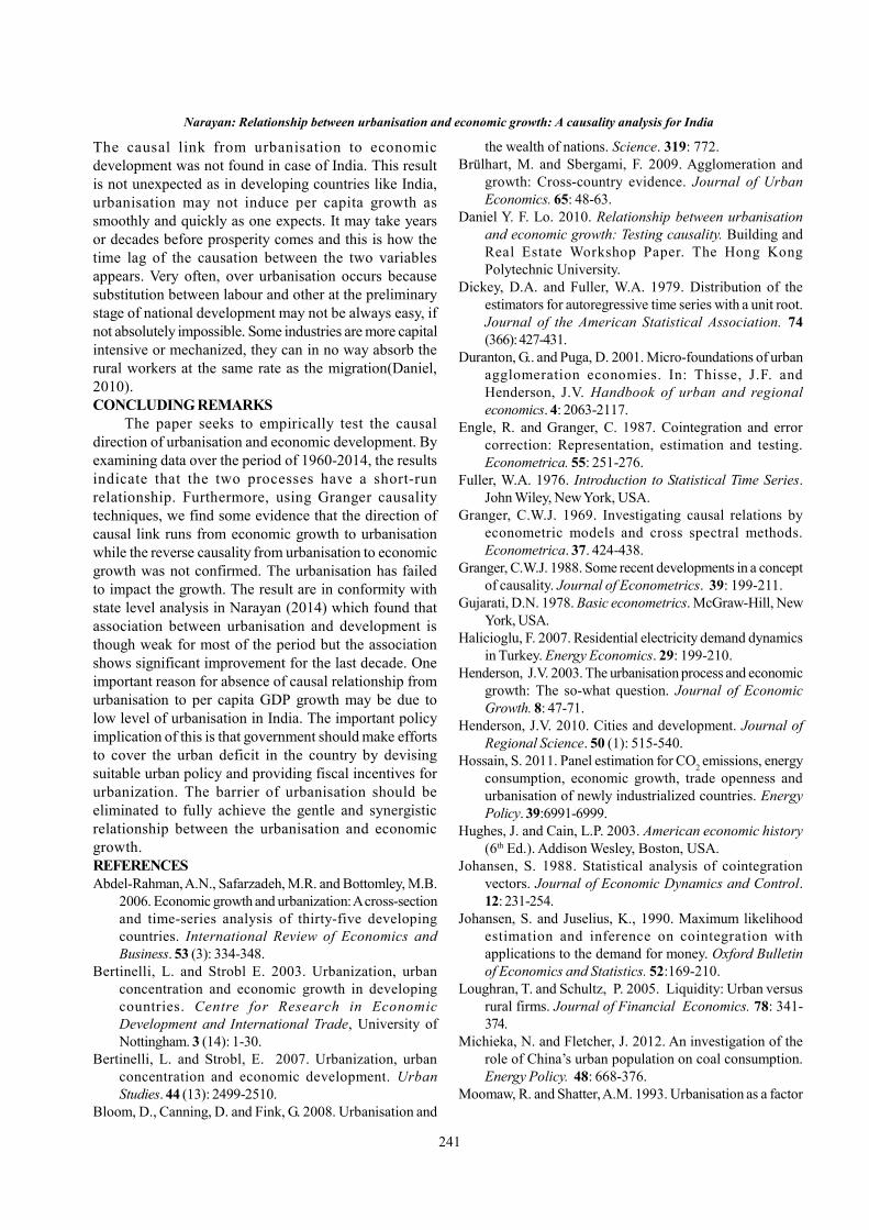
241
Narayan: Relationship between urbanisation and economic growth: A causality analysis for India
The causal link from urbanisation to economicdevelopment was not found in case of India. This resultis not unexpected as in developing countries like India,urbanisation may not induce per capita growth assmoothly and quickly as one expects. It may take yearsor decades before prosperity comes and this is how thetime lag of the causation between the two variablesappears. Very often, over urbanisation occurs becausesubstitution between labour and other at the preliminarystage of national development may not be always easy, ifnot absolutely impossible. Some industries are more capitalintensive or mechanized, they can in no way absorb therural workers at the same rate as the migration(Daniel,2010).CONCLUDING REMARKS
The paper seeks to empirically test the causaldirection of urbanisation and economic development. Byexamining data over the period of 1960-2014, the resultsindicate that the two processes have a short-runrelationship. Furthermore, using Granger causalitytechniques, we find some evidence that the direction ofcausal link runs from economic growth to urbanisationwhile the reverse causality from urbanisation to economicgrowth was not confirmed. The urbanisation has failedto impact the growth. The result are in conformity withstate level analysis in Narayan (2014) which found thatassociation between urbanisation and development isthough weak for most of the period but the associationshows significant improvement for the last decade. Oneimportant reason for absence of causal relationship fromurbanisation to per capita GDP growth may be due tolow level of urbanisation in India. The important policyimplication of this is that government should make effortsto cover the urban deficit in the country by devisingsuitable urban policy and providing fiscal incentives forurbanization. The barrier of urbanisation should beeliminated to fully achieve the gentle and synergisticrelationship between the urbanisation and economicgrowth.REFERENCESAbdel-Rahman, A.N., Safarzadeh, M.R. and Bottomley, M.B.
2006. Economic growth and urbanization: A cross-sectionand time-series analysis of thirty-five developingcountries. International Review of Economics andBusiness. 53 (3): 334-348.
Bertinelli, L. and Strobl E. 2003. Urbanization, urbanconcentration and economic growth in developingcountries. Centre for Research in EconomicDevelopment and International Trade, University ofNottingham. 3 (14): 1-30.
Bertinelli, L. and Strobl, E. 2007. Urbanization, urbanconcentration and economic development. UrbanStudies. 44 (13): 2499-2510.
Bloom, D., Canning, D. and Fink, G. 2008. Urbanisation and
the wealth of nations. Science. 319: 772.Brülhart, M. and Sbergami, F. 2009. Agglomeration and
growth: Cross-country evidence. Journal of UrbanEconomics. 65: 48-63.
Daniel Y. F. Lo. 2010. Relationship between urbanisationand economic growth: Testing causality. Building andReal Estate Workshop Paper. The Hong KongPolytechnic University.
Dickey, D.A. and Fuller, W.A. 1979. Distribution of theestimators for autoregressive time series with a unit root.Journal of the American Statistical Association. 74(366): 427-431.
Duranton, G.. and Puga, D. 2001. Micro-foundations of urbanagglomeration economies. In: Thisse, J.F. andHenderson, J.V. Handbook of urban and regionaleconomics. 4: 2063-2117.
Engle, R. and Granger, C. 1987. Cointegration and errorcorrection: Representation, estimation and testing.Econometrica. 55: 251-276.
Fuller, W.A. 1976. Introduction to Statistical Time Series.John Wiley, New York, USA.
Granger, C.W.J. 1969. Investigating causal relations byeconometric models and cross spectral methods.Econometrica. 37. 424-438.
Granger, C.W.J. 1988. Some recent developments in a conceptof causality. Journal of Econometrics. 39: 199-211.
Gujarati, D.N. 1978. Basic econometrics. McGraw-Hill, NewYork, USA.
Halicioglu, F. 2007. Residential electricity demand dynamicsin Turkey. Energy Economics. 29: 199-210.
Henderson, J.V. 2003. The urbanisation process and economicgrowth: The so-what question. Journal of EconomicGrowth. 8: 47-71.
Henderson, J.V. 2010. Cities and development. Journal ofRegional Science. 50 (1): 515-540.
Hossain, S. 2011. Panel estimation for CO2 emissions, energyconsumption, economic growth, trade openness andurbanisation of newly industrialized countries. EnergyPolicy. 39:6991-6999.
Hughes, J. and Cain, L.P. 2003. American economic history(6th Ed.). Addison Wesley, Boston, USA.
Johansen, S. 1988. Statistical analysis of cointegrationvectors. Journal of Economic Dynamics and Control.12: 231-254.
Johansen, S. and Juselius, K., 1990. Maximum likelihoodestimation and inference on cointegration withapplications to the demand for money. Oxford Bulletinof Economics and Statistics. 52:169-210.
Loughran, T. and Schultz, P. 2005. Liquidity: Urban versusrural firms. Journal of Financial Economics. 78: 341-374.
Michieka, N. and Fletcher, J. 2012. An investigation of therole of China’s urban population on coal consumption.Energy Policy. 48: 668-376.
Moomaw, R. and Shatter, A.M. 1993. Urbanisation as a factor

242
Indian J Econ Dev 12 (2): 2016 (April-June)
in economic growth. The Journal of Economics. 19 (2):1-6.
Moomaw, R. and Shatter, A M. 1996. Urbanisation andeconomic development: A bias toward larger cities?Journal of Urban Economics. 40:13-37.
Narayan, L. 2014. Urbanisation and development.International Journal of Research. 1 (8): 901-908.
Pindyck, R. and Rubinfeld, D. 1998. Econometric modelsand economic forecasts (Fourth Edition). McGraw-Hill,New York.
Rosenthal, S. and Strange, W. 2004. Evidence on the natureand sources of agglomeration economies. In:Thisse, J.F.and Henderson, J.V. (ed.) Handbook of urban and
regional economics. 4: 2119-2171.Shahbaz, M. and Lean, H. H. 2012. Does financial development
increase energy consumption? The role ofindustrialization and urbanisation in Tunisia. EnergyPolicy. 40: 473-479.
Solarin, S. and Shahbaz, M. 2013. Trivariate causality betweeneconomic growth, urbanisation and electricityconsumption in Angola: Cointegration and causalityanalysis. Energy Policy. 60: 876-884.
Wheaton, W. and Shishido, H. 1981. Urban concentration,agglomeration economies and economic development.Economic Development and Cultural Change. 30: 17-30.

243
Indian Journal of Economics and DevelopmentVolume 12 No.2: 243-248
April-June, 00000DOI: 10.5958/2322-0430.2016.00132.3
www.soed.in
Cost and Return Structure of Tomato Growers under OpenField, Low Tunnel and Poly House Conditions
Gurhemdeep Singh, J.S.Sidhu and Jasdev Singh1
Department of Economics and Sociology, Punjab Agricultural University, Ludhiana 141004 Punjab
*Corresponding author’s email:
Received: February 10, 2015 Accepted: April 24, 2016
ABSTRACTThe present investigation was carried out in the purposively selected Jandiala Guru block of Amritsar district during2013. The sample of 50 tomato growers were selected consisting of 30 open field, 10 poly house, 10 low tunnels tomatogrowers. The production and marketing practices followed by tomato growers under different methods of cultivation ledto relatively intensive use of inputs and labour in case of poly house tomato cultivation. Consequently, production andmarketing costs turned out to be higher under poly house. But due to about five times high productivity and better prices,the net returns under poly house cultivation was about seven times higher than that of open field tomato cultivation.There is further scope to enhance the productivity under poly house technology through better technical and managerialskills. At the same time, poly house technology is highly capital intensive and risky due to many constraints related toproduction and marketing. The promotion of poly house technology should be as per the demand- supply- price relationshipsof tomato, through contract cultivation integrated with processing and backed by proper insurance policy.
KeywordsCost of cultivation, protected cultivation, returns, tomato
JEL CodesM31, Q11, Q13
INTRODUCTIONTomato (Lycopersicon esculentum) is the world’s
most important productive and protective vegetable cropdue to its special nutritive value and wide spreadproduction under open field, greenhouses and net houses.Tomato is used as fresh as well as in the form ofpreserved products like ketch-up, sauce, chutney, soup,paste, puree etc. Tomato is a rich source of minerals,vitamins and organic acid, essential amino acids anddietary fibres. The world produced 163.29 million tonsof tomatoes in the year 2014-15 with the highestproduction of 51 million tonnes in China followed byIndia 18.73 million tons and America 13.8 million tons(Anonymous 2015). During 2014-15, the area andproduction of tomato in India was 9.82 million hectaresand 18.73 million tons respectively. The total area andproduction of tomatoes in Punjab was 7580 hectaresand 186.59 thousand tons respectively during 2014-15.The Amritsar district of the state has the highestproduction followed by Patiala, Kapurthala and Tarn
Taran. Protected cultivation means some level of controlover plant micro climate to alleviate one or more of abioticstress for optimum plant growth which can be achievedin poly house/net house. Production of vegetables underprotected conditions involves protection of productionstage of vegetables mainly from adverse environmentconditions such as temperature, hails, scorching sun,heavy rains, snow and frost (Singh and Vashist,1999).The production of off-season vegetable crops undernet house conditions was evaluated for total yield, earlinessand other character and incidence of insect pests. Thecultivation of vegetables in net house can play a betterrole in improving quality, advancing maturity as well asincreasing fruiting span and productivity (Cheema et al.,2004). A study on cost and return, labour employmentand marketing of vegetable crops in Jabalpur city ofMadhya Pradeshindicated that net returns from tomatowere the highest with `2037 per acre and the producer’sshare in the consumer’s rupee in the marketing ofvegetables worked out to be 42 per cent (Mishra and

244
Indian J Econ Dev 12 (2): 2016 (April-June)
Saraf 1987). Thakur et al. (1997) conducted a study ofseasonal vegetable in Kullu and found that the total costof production was higher for tomato followed bycauliflower, cabbage and capsicum. The net profits were`145961, `73900, `68246, `46266 and `44777 perhectare from tomato, cauliflower, cabbage, capsicum andpea respectively, in Himachal Pradesh. Sharma et al.(2000) examined tha income and the employment fromsummer vegetables vis-à-vis their competing crop (paddy)in Punjab. The results show that tomato crop was mostcapital intensive with an expenditure of `31642 perhectare against sponge gourd which was `16072 perhectare. The returns over production cost were highestfor tomato crop followed by capsicum and brinjal.
A study on economics of production and marketingof vegetables in Karim Nagar district of Andhra Pradeshrevealed that though’ the cost of cultivation was highestin tomato with `28055 per hectare yet net returns werehigh in cauliflower with `55792 per hectare followed bytomato with `49758 per hectare. The cost benefit ratiowas highest for cauliflower (1:2.90) and lowest for bhindicrop (1:0.28) (Radha and Prasad, 2001). Thyagarajan etal. (2005) studied the recommended technologies adoptedby the tomato growers of Tamil Nadu. They reportedthat the tomato growers faced the problems such as wideprice fluctuations, lack of knowledge to identify pestsand diseases, high cost of labour, inadequate water supply,non-availability of credit, exploitation by the middlemenby charging heavy rate of commission and brokerage,lack of adequate transport and market facilities and lackof storage facilities at the village level in the descendingorder. They suggested fixing a minimum economic pricefor tomato throughout the entire season, arrangingintensive training programs for tomato growers especiallycovering identification of pests and diseases, scientificstorage and educating the farm labourers through theirleaders. Singh and Asrey (2005) studied the performanceof tomato and sweet pepper under unheated greenhouse.Thus, the studies have indicated that cultivation oftomato and sweet pepper under green house would notonly help in getting higher productivity but also fetchbetter returns. Anonymous (2006) reported that Net houseis necessary to produce good quality vegetables and obtainhigher yields. The budget for vegetable cultivation in thenet house shows that a small farmer (with capital subsidyassistance including some risk coverage) starting from0.5 acre can earn more than `1 lakh per year. Singh andSirohi (2008) found that protected cultivation vegetablesoffers distinct advantages of quality, productivity andfavorable market price to the growers. Vegetable growerscan substantially increase their income by protectedcultivation of vegetables in off-season as the vegetablesproduced during their normal season generally do not get
good returns due to large availability of these vegetablesin the markets. According to Wani et al. (2011)greenhouses were the most efficient means to overcomeclimatic diversity. Greenhouse vegetable production makethe use of recent advances in technology to control theenvironment for maximizing crop productivity percentarea and increasing the quality of vegetables produce.India has entered into the area of greenhouse vegetablescultivation more recently and the total area under protectedvegetable production is not more than 10,000 ha. Thegreenhouse technology is still in its preliminary stage inIndia and concerted efforts are required from allconcerned agencies to bring it at par with the globalstandards. Economically viable and technologically feasiblegreenhouse technology suitable for the Indian agro-climatic and geographical conditions is needed at theearliest (Nair and Brache, 2014). Warner (1991) conducteda study in the German Republic to examine the prospectfor improving farm income from vegetable farming. Theresult showed that income from vegetable farming wasmuch higher than the income from traditional agriculturalproduction.METHODOLOGY
The study was conducted in Amritsar city during2014-15. The Jandiala Guru block of Amritsar districtwas purposively selected on the basis of highestconcentration of diverse population of tomato growers.From the selected block, ten villages having at least onepoly house and some open field and low tunnel growerswere selected .From the selected ten villages a sample of50 respondents in the ratio of 3:1:1 that is 3 open fieldfarmers and one each poly house and low tunnel tomatogrowers were selected. Primary data was collectedthrough a pre-tested and well-structured questionnaireRESULTSAND DISCUSSIONComparative cost and return under open field, lowtunnel and poly house tomato cultivation
The perusal of Table 1 depicted the composition ofproduction and marketing cost per acre in poly house,open field and low tunnel cultivation of the selected tomatocultivators. In the case of open field cultivation of tomato,the variable cost was worked out to be `27698/acre,accounting for 77.33 percent of the total variable costand the remaining 22.67 percent was the marketing costwhich was `8118. The total variable cost was `35816. Itwas observed that the highest proportion was spent onlabour with 21.61 percent followed by plant protection,seed, fertilizers, machinery and irrigation charges with20.26, 14.97, 10.68, 9.73 and 0.08 percent, respectively.
The production variable cost in poly house cultivationof tomato was worked out to be `165155/acre,accounting 78.50 percent and the remaining 21.50 percentof the total variable cost was marketing cost. The variable
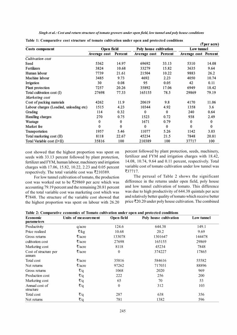
245
cost showed that the highest proportion was spent onseeds with 33.13 percent followed by plant protection,fertilizer and FYM, human labour, machinery and irrigationcharges with 17.06, 15.82, 10.22, 2.23 and 0.05 percentrespectively. The total variable cost was `210389.
For low tunnel cultivation of tomato, the productioncost was worked out to be `29869 per acre which wasaccounting 79.19 percent and the remaining 20.81 percentof the total variable cost was marketing cost which was`7848. The structure of the variable cost showed thatthe highest proportion was spent on labour with 26.20
Table 1: Comparative cost structure of tomato cultivation under open and protected conditions(`per acre)
Costs component Open field Poly house cultivation Low tunnelAverage cost Percent Average cost Percent Average cost Percent
Cultivation costSeed 5362 14.97 69692 33.13 5310 14.08Fertilizers 3824 10.68 33279 15.82 3635 9.64Human labour 7739 21.61 21504 10.22 9883 26.2Machine labour 3485 9.73 4692 2.23 4050 10.74Irrigation 30 0.08 95 0.05 42 0.11Plant protection 7257 20.26 35892 17.06 6949 18.42Total cultivation cost (I) 27698 77.33 165155 78.5 29869 79.19Marketing costCost of packing materials 4262 11.9 20619 9.8 4170 11.06Labour charges (Loadind, unloading etc) 1515 4.23 10344 4.92 1358 3.6Grading 114 0.32 0 0 240 0.64Handling charges 270 0.75 1523 0.72 938 2.49Wastage 0 0 1671 0.79 0 0Market fee 0 0 0 0 0 0Transportation 1957 5.46 11077 5.26 1142 3.03Total marketing cost (II) 8118 22.67 45234 21.5 7848 20.81Total Variable cost (I+II) 35816 100 210389 100 37717 100
percent followed by plant protection, seeds, machinery,fertilizer and FYM and irrigation charges with 18.42,14.08, 10.74, 9.64 and 0.11 percent, respectively. Totalvariable cost of tomato cultivation under low tunnel was`37717.
The perusal of Table 2 shows the significantdifference in the returns under open field, poly houseand low tunnel cultivation of tomato. This differencewas due to high productivity of 644.38 quintals per acreand relatively better quality of tomato which receive betterprice `20.20 under poly house cultivation. The combined
Singh et al.: Cost and return structure of tomato growers under open field, low tunnel and poly house conditions
Table 2: Comparative economics of Tomato cultivation under open and protected conditionsEconomicparameters
Units of measurement Open field Poly house cultivation Low tunnel
Productivity q/acre 124.6 644.38 149.1Price realized `/kg 10.68 20.2 9.69Gross returns `/acre 133078 1301647 144478cultivation cost `/acre 27698 165155 29869Marketing cost `/acre 8118 45234 7848Cost of structure perannum
`/acre 0 374227 17865
Total cost `/acre 35816 584616 55582Net returns `/acre 97262 717031 88896Gross returns `/q 1068 2020 969Production cost `/q 222 256 200Marketing cost `/q 65 70 53Annual cost ofstructure
`/q 0 312 103
Total cost `/q 287 638 356Net returns `/q 781 1382 596

246
Indian J Econ Dev 12 (2): 2016 (April-June)
effect resulted into high gross return of `1301692. Underopen field the average per acre production was 124.60quintals and realized price of `10.68 and the gross returnwas `133021. For low tunnel, the production was slightlymore than open field because of early sowing. It hadproduction of 149.10 quintals per acre with the realizedprice of `9.69 and the gross return worked out to be`144478. The low price realization under low tunnel wasdue to the attack of blight due to covering, to protectfrom frost which resulted in high moisture content andleads to abnormal growth and relatively poor quality fruitinspite of better yield. The total cost worked out in caseof open field, poly house and low tunnel was `35816,`584616 and `55582 respectively. Net return was highestfor poly house that was `717031 followed by `97262under open field and `88896 under low tunnel.Comparative economics of open field tomato-paddycrop rotation and poly house tomato cultivation
The cropping pattern of all three tomato growerswere given in the Table 3. The duration of crop underopen field and low tunnel was five months from Januaryto mid- June and for poly house it was nine months fromNovember to August and the poly house remained fellowfor the rest of the months to prepare it for the next tomatocrop. Open field and low tunnel growers grew paddyafter tomato crop. The Table 3 presents the comparativeannual economics of open field and low tunnel tomatogrowers under tomato- paddy rotation with poly housecultivation. The gross return per acre for open field undertomato-paddy rotation was `168048 and total cost was`55666 and so net return was `112382. For low tunnelsthe gross return was `179448 and total cost was `75432and net return was `104016. For the poly house the netreturns was `717031 over the total cost of `584616 andgross return was of `1301647. The lowest profitabilitywas under low tunnel due to high attack of fungus atearly stages, which effect quality as well as quantity ofthe fruit and hence less price. The annual net return inthe case of poly house cultivation was about seven timesthe net returns under unprotected cultivation. But poly
house technique requires high inputs, managerial andtechnical skills along with high initial investment.Comparative analysis of lowest, medium and highestreturn poly house tomato growers
In order to examine the potential of net returns underpoly house cultivation of tomato growers with lowest,medium and highest returns were segregated and theircomparative economics is presented in Table 4. The tableshowed that the lowest return grower got the productivityof 352 quintals and realized price of `2000 per quintal.His total cost of cultivation cost was `100510 andmarketing costs was `40520. The annual value of materialwas `374227 and total cost was `515257. The grossreturns were `704000 and net return was `188743. Themedium return grower used hybrid plants along withbetter quality inputs which result in relatively higher costof cultivation of `228206 and marketing cost of `71370.The annual fixed structure cost was same as `374227and the total cost was `673803. The productivity in caseof medium return grower was 580 quintals and he gotthe same price `2000 per quintal. The gross return was`1160000 and net return was `486197. The mediumreturn grower though got high productivity at high costdue to the attack of blight in the early stage which resultedretransplanting of the plants which costs him double andalso due to fungus attack, the high use of plant protectionmaterial also added to his production cost. More volumeof the produce increased the marketing cost also but stillgot more net returns as compared to low return growers.
The highest return tomato grower under poly housegot 730 quintals of tomato per acre realized better priceof `2200 per quintal. He imported the plant from Germancompany at the cost of `8 per plant and for 12000 plantshis cost was `96000. The production costed him `224265and marketing costed him `88750. High production ledto more number of picking and visits to the markets whichincreased the marketing cost. The total cost was `514197and gross return was `1606000 and net return was`918758. Due to good managerial skills and hightechnological production practices followed by high returngrower resulted in high production and also fetched betterprices for his produce. One case of a grower who closedhis poly house was also examined in order to know thereasons for the shutdown. The farmer had been doingprotected cultivation since last 8 years he used to cultivatetomato, capsicum, lilium, and gerbera. He had been usinghigh technological methods of cultivation. But during2012, he got 350 quintals of tomato and he sold at priceof `1700 per quintal. The total cost was `576052 andgross return was `595000 with net return only at `18948.The major reason was that due to high humidity andrainfalls, the attack of fungus along with sun scalp wasvery severe resulted into rottening of tomato fruit which
Table 3: Economics of tomato cultivation under protectedand open field with different crop-rotation
(`acre -1)Particulars Crop Gross
returnsTotalcost
Netreturns
Open field (Tomato-paddy rotation)
Tomato 133078 35816 97262Paddy 34970 19850 15120Total 168048 55666 112382
Poly house cultivation OnlyTomato
1301647 584616 717031
Low tunnel (Tomato-paddy rotation)
Tomato 144478 55582 88896Paddy 34970 19850 15120Total 179448 75432 104016

247
reduced the quality and hence got lower prices. At thesame time with the stormy weather and high velocitywinds, the poly sheet which was not of the desirablequality as described under government guidelines wascompletely destroyed. This adverse experience resultedin huge loss to the farmer and ultimately led to the decisionto shut down his protected cultivation.CONCLUSIONS
The use of inputs and labour employment was morein case of poly house than in open field and low tunnelcultivation of tomato. Consequently, the total costs ofproduction and marketing along with initial investmentwas very high under protective technique. At the sametime the gross returns and net returns of tomato underprotected cultivation were many times high as comparedto open field cultivation due to high productivity and goodquality of fruits. For the low tunnel the grower’s reactionwas not favorable due to high attack of blight. The qualityof fruit was also very poor resulting in low yield andprice.The management and technical skills played a keyrole in attaining high returns from the poly house
technology. It also faced many constraints as well asrisks and need constant monitoring and supervision. Anynegligence at any stage may render the whole poly housetechnology unviable as indicated by the case study of ashutdown experience of a farmer. Finally, poly housetechnology of vegetable growing is not everybody’sbusiness. It can be successfully adopted by highlymotivated, well trained and resourceful farmers along withdeveloped marketing and insurance system. It should haveintegrated with processing of tomato through contractfarming. Above all, the promoters should keep in mindthe commodity outlook in term of demand, supply andprice relationships. Which are highly sensitive in case ofvegetables in general and particularly for tomato crop.REFERENCESAnonymous. 2006. Agricultural and rural development of
Punjab. The Punjab State Farmers Commission,Government of Punjab, Mohali: 43-44.
Anonymous. 2015 Report on vegetables production.Horticulture Department. Government of Punjab,Chandigarh.
Cheema, D.S., Kaur, P., and Kaur, S. 2004. International
Singh et al.: Cost and return structure of tomato growers under open field, low tunnel and poly house conditions
Table 4: Economics of tomato cultivation in poly house with respect to low, medium, high and closed poly house productivityand returns
(`acre -1)Particulars Average cost
Low Medium High Closed downProduction costSeed 4800 99200 96000 61650Fertilizers 13400 26300 28700 30250Human labour 51450 54826 62625 20500Machine labour 4000 5000 4000 5500Irrigation 60 80 40 105Plant protection 26800 42800 32900 35450Total production cost (I) 100510 228206 224265 153455Marketing costCost of packing materials 25000 37500 32250 20250Labour charges 3520 6820 13500 10350Grading 0 0 0 0Handling charges 0 7050 19000 2500Wastage 0 0 0 0Market fee 0 0 0 0Transportation 12000 20000 24000 15250Total marketing cost (II) 40520 71370 88750 48350Total cost (I+II) 141030 299576 313015 201805Material cost 374227 374227 374227 374227Total cost 515257 673803 687242 576052ReturnsProductivity (qacre-1) 352 580 730 350Average price (` per q) 2000 2000 2200 1700Gross returns 704000 1160000 1606000 595000Total cost 515257 673803 687242 576052Net returns 188743 486197 918758 18948

248
Indian J Econ Dev 12 (2): 2016 (April-June)
symposium on protected cultivation in mild winterclimates: Production, pest management and globalcompetition. ISHS Acta Horticulture. 60:659.
Mishra, R.S. and Saraf, G.P. 1987. Cost and returns, labouremployment and marketing of vegetable crops in Jabalpurcity of Madhya Pradesh. Indian Journal of AgriculturalEconomics. 42 (4): 462-463.
Nair, R. and Brache, S. 2014. Protected cultivation ofvegetables-Present status and future prospects in India.Indian Journal of Applied Research. 4 (6): 245-247.
Radha, Y. and Parsad, E.Y. 2001 Economics of production andmarketing of vegetables in Karim Nagar district AndhraPradesh. Indian Journal of Agricultural Marketing 15:61-65.
Sharma, V.K., Sain, I., and Singh, G. 2000. Income andemployment from summer vegetables vis-à-vis theircompeting crop paddy in Punjab. Journal ofAgricultural Development and Policy 12: 38-43.
Singh, B. and Sirohi, N.P.S. 2008. Protected cultivation ofvegetables in India: Problems and future prospects. ActaHorticulture : 710.
Singh, K. and Vashist, G. D. 1999. An analysis of production
and marketing system of vegetable in Lambagaon blockof district Kangra (H.P.). The Bihar Journal ofAgricultural Marketing. 7: 376-389.
Singh, R. and Asrey, R. 2005. Performance of tomato andsweet pepper under unheated green house. HaryanaJournal of Horticulture Science 34 (1-2): 175.
Thakur, D., Lal, S.H., Thakur, D.R., Sharma, K.D., and Saini,A.S. 1997. Market supply response and marketing problemof farmers in the hills. Indian Journal of AgriculturalEconomics. 52: 139-150.
Thyagarajan, S. and Prabu, R. 2005. Recommendedtechnologies adopted by tomato growers. AgriculturalExtension Review. 17: 26-30.
Wani, K., Singh, P., Amin, A., Mushtaq, F., and Dar, Z. 2012.Protected cultivation of tomato, capsicum and cucumberunder Kashmir Valley conditions. S.K. University ofAgricultural Sciences and Technology of Kashmir. 58:246-249.
Werner, R. 1991. The income prospects of vegetable growingin close proximity to the market. Institute fur landWirtschaffluche Belnelislulzre del’ UniversitalMohenheul. 68: 393-403.

249
Indian Journal of Economics and DevelopmentVolume 12 No.(2): 249-254
April-June, 2016DOI: 10.5958/2322-0430.2016.00133.5
www.soed.in
Composition, Intensity and Competitiveness of AgriculturalTrade between India and ASEANRenjini V.R.* and Amit Kar
Division of Agricultural Economics, Indian Agricultural Research Institute, New Delhi, 110012
*Corresponding author’s email: [email protected]
Received: March 18, 2016 Accepted: May 25, 2016
ABSTRACTAn attempt was made to study the current status, composition, intensity and competitiveness of agricultural trade betweenIndia and the ASEAN for the period 1995-2014. The results revealed that, more than 10 percent of export and 30-40percent of import were directed to the ASEAN in comparison to world. Vietnam and Indonesia were found to be majorexport destination and source of agricultural commodities respectively. The ASEAN continued to be the most preferredtrading partner of India with a trade intensity index value of more than two for all the considered years. India hadmaintained higher trade intensity with Indonesia, Malaysia, Thailand, Vietnam and Myanmar compared to Brunei,Cambodia and Lao. India maintained competitiveness in marine products, spices, rice and oilcake meals over China,Australia and USA which are the major agricultural exporters to the ASEAN considered in the study. But, China hasemerged as a tough competitor to India in cotton, fruits, vegetable and coffee in the ASEAN market that point out the needof increasing the export competitiveness of the agricultural commodities.
KeywordsASEAN, export intensity, import intensity, Revealed Comparative Advantages
JEL CodesF00, F02, F13, F15, F19
INTRODUCTIONIndia’s relationship with the Association of South
East Asian Nations (ASEAN) countries commenced as apart of her “Look East” policy during economic reformera. Though India had a long term trade relationship withASEAN countries, bilateral trade has been intensified afterIndia became sectoral dialogue partner in 1992 andconsequently full dialogue partner in 1995. Since thenbilateral relationships has been extended to several sectorslike trade, science and technology, agriculture,environment, human resource development, informationand communication technology, tourism and culture, etc.(Kuppuswami, 2010).
ASEAN, which is a geo-political and economicorganization of ten South East Asian countries, came intoexistence in August 1967. Indonesia, Malaysia, thePhilippines, Singapore and Thailand were the foundercountries. Later, Brunei Darussalam, Cambodia, the LaoPeople’s Democratic Republic, Myanmar and Vietnamalso joined the association. ASEAN was the seventh largesteconomy in world and third largest economy in Asia with
a combined GDP of US$ 2.6 trillion in 2014 (ASEANTrade Statistics, 2014). It is the third largest market inthe world, after China, and India serving over 600 millionpopulations. Total trade of the ASEAN increased nearlyby US $ 1 trillion between 2007 and 2014, with a greatershare in intra regional trade proving it as the mostintegrated market. The combined average real GDP ofthe ASEAN countries during 2008-11 was 5.5 percent ascompared to the world GDP growth of 2.8 per cent. TheASEAN Economic Community formed in 2015, is anotheramong the steps to increase the integration to benefit allmember countries (Plummer et al., 2014).
The ASEAN India Free Trade Agreement (AIFTA)is considered as one of the world’s largest Free TradeAgreement that covers a market of nearly 1.8 billion peoplewith a combined GDP of US$ 2.8 trillion. It proposes togradually slash tariffs for about 4,000 product lines overa staggered period, by 2016. India is the tenth largestexport destination of ASEAN with a share of 3.4 per centin total exports. Also, 2.1 per cent of total ASEAN importsoriginate in India contributing to 2.7 percent share in total

250
Indian J Econ Dev 12 (2): 2016 (April-June)
trade with ASEAN. In addition, the ASEAN- India bilateraltrade has increased by several times from US$ 2.9 billionin 1993 to US$ 67.9 billion in 2014 (ASEAN TradeStatistics, 2014). At present, both the sides expect that,the bilateral trade among them will increase to $200 billionwithin a decade. These numbers suggests the substantialopportunity for India to improve and expand its tradingrelations within the ASEAN. In this scenario, an attemptis made here to study the present status, compositionand trade intensity among India and the ASEAN countries.Besides, India’s export competitiveness in selectedagricultural commodities were calculated and comparedwith the other major agricultural exporters to ASEANnamely China, USA and Australia.DATA BASEAND METHODOLOGY
The study was based on secondary data fromvarious sources. The bilateral agriculture trade data wereobtained from United Nations COMTRADE database andInternational Trade Centre Trade Map website for theperiod 1995 to 2014. Percentage shares and growth ratehas been worked out to get the composition and statusof agricultural trade between India and ASEAN countries.
Trade Intensity Index (TII) measures werecalculated to see the degree of trade relationship betweenIndia and the ASEAN. Further, Export Intensity Index(EII) and Import Intensity Index (III) were calculated tosee the extent to which the country prefers to trade withthe ASEAN in comparison to rest of the world. The indexcan be expressed as:Export Intensity Index (EII)
IWA
IIA
M-MMXX
countriesASEANandIndiabetweenEII =
XIA = Value of India’s agricultural export to ASEAN countriesXI = India’s total agricultural exportMA = Total agricultural import by ASEAN countriesMW = Total world’s agricultural importMI = India’s total agricultural import
Import Intensity Index (III)
)X-X(XMM
countriesASEANandIndiabetweenIIIIWA
IIA=
MIA= India’s agricultural import from ASEAN countriesMI = India’s total agricultural importXA = Total agricultural export of ASEAN countriesXW = Total world’s agricultural export
XI = India’s total agricultural exportAn index of greater (less) than unity indicates larger
(smaller) than expected trade flow between two parties.Revealed Comparative Advantage (RCA)
India’s competitiveness in export of agriculturalcommodities to ASEAN in comparison with that of other
major trading partners of ASEAN like Australia, Chinaand USA was calculated by calculating RevealedComparative Advantage Index. The index is expressedas:
)1965(Balassa.........XXXX
RCAAiA
BiB=
Where,XiB= India’s export of commodity ‘i’ to ASEANXB = India’s total agricultural export to ASEANXiA= The rival country’s export of commodity ‘i’ to ASEANXA = The rival country’s total agricultural export to ASEAN
A positive value of RCA indicates better comparativeadvantage for India as compared to other competingcountries in the ASEAN market.RESULTS AND DISCUSSIONStatus and Composition of Agricultural Tradebetween India and ASEAN
The agricultural trade between India and ASEAN,in comparison to the rest of world, is depicted in table1.It shows that, on an average, from 1995 to 2014, morethan ten per cent of India’s agricultural export to worldwas directed towards ASEAN countries. Agriculturalexport to ASEAN has steadily increased during the periodexcept in 2012. In the case of import, an average of 30-40 per cent of agricultural commodities were sourcedfrom ASEAN countries during this period. Emergence ofIndia as a major market for agricultural commodities ofASEAN can be observed in light of the increased shareof agricultural imports. The share of agricultural exportin total export has decreased from 31.32 percent in 1995to 13.32 per cent in 2005 after which it showed anincreasing trend. The same trend can be observed inagricultural import also. The percentage share ofagricultural trade between India and the ASEAN againpicked up the momentum from 2010 onwards, just afterthe implementation of free trade agreement, which is apositive sign. While total merchandise export and importwith ASEAN has grown by 10.96 per cent and 11.61 percent respectively during 1995-2010, agricultural exportand import grew at a slower pace of 6.80 per cent and7.50 per cent respectively. Thus, it is clear that agriculturalimport from ASEAN was always at a higher level thanexport.
During triennium ending 2014, India has exportedagricultural commodities worth US$ 8560.65 million andimported commodities worth US$ 9567.46 million, thusshowing a deficit in trade (Table 2). India’s major exportdestination was Vietnam with a share of around 47 percent in total agricultural exports worth US dollar4021.21million. Malaysia, Indonesia, and Thailand also

251
Renjini and Kar: Composition, intensity and competitiveness of agricultural trade between India and ASEAN
received a significant share of 15, 14, and 12 percentrespectively in exports. Indonesia stood first among thesource of agricultural import for India with a share ofaround 57 per cent in total agricultural import fromASEAN. Malaysia was the second largest source of import(25 percent) and a considerable volume of imports werealso sourced from Myanmar (7.19 percent), Thailand(4.94 percent) and Vietnam (4.52 percent) during thisperiod (Table 2). It is clear that, in triennium ending 2014,around 80 per cent of India’s agricultural trade wasconcentrated in Indonesia, Malaysia and Vietnam. India’sagricultural trade with less developed countries of ASEANlike Brunei, Cambodia and Lao was observed low duringthe study period with less than one per cent share in totalagricultural trade.
Composition of India’s agricultural trade with majorASEAN members provides better picture of bilateral trade.India’s export basket consisted of meat and edible meatoffal, fishery products, edible vegetables, cereals, coffee,tea, mate and spices, oilseeds, cotton, residues, and wasteof food industry, having more than one per cent share intotal agricultural export to ASEAN in triennium ending2014 (Table 3). Further, these commodities togetherconstituted more than 90 percent of the total agriculturalexport to ASEAN during this period. Vietnam holds
significant share in the import of these commoditiesmaking it the most preferred market for Indian agriculturalcommodities. Meat and edible meat offal is the majorexport item constituting 29 percent in total agriculturalexport to the ASEAN of which more than 60 percentwas exported to Vietnam due to the huge demand forbuffalo meat from the country. The cereals accounts for14 percent of the total agricultural export which is mainlydestined to Indonesia (39 percent), Malaysia (21 percent)and Vietnam (21 percent). Maize, wheat and non- basmatirice were the major cereals demanded in these countriesduring this period.
Vietnam, Thailand, and Malaysia were the mostpreferred destinations for export of fish products with acombined share of 94 percent in total fish products export.About 26 percent of tobacco export, mainly Flue CuredVirginia variety, was directed towards Philippines,followed by Singapore (17 percent) and Vietnam (17percent). Other important items in Indian export basketwere oilseeds (9 percent), residues of food industry (8.68percent), cotton (8.06 percent), coffee, and tea, mateand spices (5 percent). Vietnam and Indonesia togetherhave a share of more than 60 percent oilseeds importfrom India in 2014. Again, more than 40 percent of thecotton export to ASEAN was directed towards Vietnamdue to their increased demand in domestic garment andtextile sector.
Animal and vegetable oil was the dominated item in2014 with a share of 77 percent in total agricultural importof India from ASEAN (Table 4). Palm oil was the majorimported form under this category in this period whichwas mainly supplied by major producers of the world,Indonesia and Malaysia. The share of each country inIndia’s import of this commodity was 60 percent and 38per cent respectively. The neighbouring country Myanmaris the largest source of India’s edible vegetable. Duringthe same period, out of 7 percent of vegetable import byIndia from ASEAN, 99 percent was sourced fromMyanmar.
Apart from export, India considerably imports
Table 2: Country wise distributions of agricultural tradebetween India and ASEAN during triennium ending 2014
($ millions, Share in percent)Country Export Share Import Share Total ShareBrunei 16.80 0.20 0.09 0.00 16.89 0.09Cambodia 50.64 0.59 3.43 0.04 54.06 0.30Indonesia 1204.65 14.07 5433.97 56.80 6638.62 36.62Lao 19.40 0.23 0.10 0.00 19.50 0.11Malaysia 1326.16 15.49 2432.68 25.43 3758.84 20.73Myanmar 140.60 1.64 688.25 7.19 828.85 4.57Philippines 386.82 4.52 28.02 0.29 414.83 2.29Singapore 362.59 4.24 76.35 0.80 438.94 2.42Thailand 1031.79 12.05 472.28 4.94 1504.07 8.30Vietnam 4021.21 46.97 432.30 4.52 4453.51 24.57TotalASEAN
8560.65 100.00 9567.46 100.00 18128.12 100.00
Table 1: Agricultural trade between India and ASEAN, 1995-2014Particulars 1995 2000 2005 2010 2011 2012 2013 2014Agri export to ASEAN as a percent of export to world 8.45 9.71 10.11 13.92 16.07 14.91 17.11 18.14Agri import from ASEAN as a percent of import from world 35.28 40.14 30.19 43.38 46.78 47.91 45.91 40.63Agri export as a percent of total export to ASEAN 31.32 32.32 13.32 16.74 18.37 22.12 25.25 28.68Agri import as a percent of total import from ASEAN 31.65 29.06 18.44 21.83 21.05 23.66 22.11 20.77Growth in trade between India and ASEAN 1995-2014 (percent )Total export 11.61Total import 10.96Agri export 6.80Agri import 7.50Computed based on UNCOMTRADE database

252
Indian J Econ Dev 12 (2): 2016 (April-June)
coffee, tea, mate and spices also, which togetherconstituted around 3 percent share in total agriculturalimport from the ASEAN during the period. Vietnamsupplied 71 percent of coffee, tea, mate and spices toIndia whereas, 23 per cent import share goes to Indonesia.Even though India stands fifth in world in the productionof natural rubber, domestic demand has been increasingovertime and the commodity is mainly imported fromASEAN countries. Indonesia supplied 47 percent of thenatural rubber to India followed by Thailand (27 percent)and Vietnam (20 percent).Agricultural Trade Intensity between India andASEAN Countries
India’s agricultural export intensity and importintensity with the ASEAN as a whole were found to behigher than two in all the years (Table 5). It clearlyindicates that, India have strong trade relationship withthe ASEAN compared with that of world. However, India’simport intensity is higher than the export intensity
because, ASEAN exported more to India than imports. Itcan be inferred that, India exports much less to ASEANmarket than what it should be and ASEAN imports muchless from the Indian market than what it should be. Thecountry wise trade intensity showed that, India’s exportintensity was more than one for all the years for Indonesia,Malaysia, Thailand and Vietnam. India’s export intensityindex with Vietnam was found to be higher compared toother countries. Export intensity index began to rise in2000s for Cambodia, Philippines but followed a fluctuatingtrend. India had significant export intensity with Myanmarafter signing free trade agreement in 2010. Export intensityindex however started to decline post FTA for Singaporeshowing India’s changing market preference to otherASEAN countries. India had lesser export intensity withBrunei and Lao for all the years considered except in2014.
Import intensity index, also the indicator of demandof the agricultural products of ASEAN, revealed that,
Table 3: Composition of India's agricultural export to ASEAN, TE 2014HS code Commodity TE 2014
(‘000 $)Percent share of top 3 countries in India'sexport of respective commodities
2 Meat and edible meat offal 2510919.3(29.33)
Vietnam (67), Malaysia (15), Thailand (11)
3 Fish, crustaceans, molluscs, aquatic invertebrates nes 1092257.7(12.76)
Vietnam (84), Thailand (5), Malaysia (5)
7 Edible vegetables and certain roots and tubers 167294.67(1.95)
Malaysia (60), Indonesia (14), Singapore (10)
9 Coffee, tea, mate and spices 429397(5.02)
Vietnam (41), Malaysia (28), Thailand (17)
10 Cereals 1232687.70 (14.40)
Indonesia (39), Malaysia (21), Vietnam (21)
12 Oil seed, oleagic fruits, grain, seed, fruit, etc. 782306.00 (9.14)
Vietnam (34), Indonesia (32), Malaysia (13)
23 Residues, wastes of food industry, animal fodder 742625.33(8.68)
Vietnam (34), Thailand (33) Indonesia (16),
24 Tobacco and manufactured tobacco substitutes 134225.33(1.57)
Philippines (26), Singapore (17) Vietnam (17),
41 Raw hides and skins (other than fur skins) and leather 193110.33(2.26)
Vietnam (44), Malaysia (23) Indonesia (12),
52 Cotton 690107.33(8.06)
Vietnam (47), Indonesia (18), Thailand (10)
Other agricultural commodities 585721(6.84)
Total 8560651.67Computed based on UNCOMTRADE databaseFigures in parentheses (3rd column) are percentage to the total agricultural export to ASEAN
Table 4: Composition of India's agricultural import from ASEAN in TE 2014HS code Commodity TE 2014
(‘000 $)Percent share of top 3 countries in India'simport of respective commodities
7 Edible vegetables and certain roots, and tubers 680073.00 (7.11) Myanmar (99), Indonesia (0.3), Thailand (0.2)9 Coffee, tea, mate, and spices 243666.33 (2.55) Vietnam (71) Indonesia (23), Singapore (4)15 Animal, vegetable fats and oils, cleavage products, etc. 7342682.00 (76.76) Indonesia (60), Malaysia (38), Thailand (1)4001 Natural rubber, balata, gutta-percha, etc. 820035.67 (8.57) Indonesia (47), Thailand (27) Vietnam (20)
Others 430588 (5.02)Total 9567464.67Computed based on UNCOMTRADE database, Figures in parentheses (3rd column) are percentage to the total agricultural import from ASEAN

253
Renjini and Kar: Composition, intensity and competitiveness of agricultural trade between India and ASEAN
countries like Indonesia, Malaysia and Myanmar hadintensity value greater than one in all the considered years(Table 5). Myanmar which shares border with India,occupied the highest position in import intensity indexwith a double digit intensity value during the period understudy. Import intensity index for Cambodia was lowerin the period except in 2010 and 2011, whereas for Laoand Philippines the index remained less than one in all theconsidered years. Agricultural trade with Lao was meagerwhich might be due to its peculiar geographical naturewith difficulties in transportation and market expansion.
world; China holds comparative advantage in ASEANmarket in all the years of the study. As leading exportersof cotton in the world, USA and Australia also stood ascompetitors in cotton supply to ASEAN market till 2012with the exception in 2010. There is a substantialopportunity for India in ASEAN market in cotton exportto cater the demand of growing textile industries incountries like Vietnam and Indonesia. But, gainingcomparative advantage over major competitor China, inexport of key commodity like cotton in ASEAN marketis a matter of concern. It is clear from the results that,
India enjoyed monopoly in marine products exportin all the years as there is wide demand for the Indianfisheries products in ASEAN countries. China heldcompetitive position in export of vegetables to ASEANcountries, while India maintained comparativeadvantage over USA and Australia during the periodunder study. India doesn’t have any comparativeadvantage in export of fruits to the ASEAN marketbecause Indian fruits exports are mainly directedtowards neighbouring and gulf countries. As Indiahas emerged as net exporter of oil meals, it couldmaintain a superior status in export of oilcake mealsin ASEAN market without facing any competitionfrom other countries considered in the study. Beingthe second largest producer of tea, India hadadvantage over Australia and USA, while it facedcompetition from top producer cum exporter China,in all the years. Increased domestic demand in Indiaand ASEAN’s growing preference to green tea mighthave favoured China, which is a major supplier ofgreen tea to ASEAN.
In the case of coffee, India had comparativeadvantage over Australia and China till 2005, later onit lost the competency while, it could compete withUSA only in the year 1995. India, being largestproducer and exporter, maintained comparativeadvantage in export of spices over three countries in
which China was a competitor only in 1995. The higherpreference to Indian spice varieties in ASEAN countrieshad given substantial opportunities for India to competewith China. Being largest exporter of tobacco in the world,USA didn’t stand as a competitor for India after 2000,while China continued to be competitor against India inASEAN market. Australia and USA which are the majorexporters of dairy products globally, have maintained acompetitive position against India in ASEAN marketwhereas, India could dominate China in export of dairyproducts in most of the years. As a net exporter of rice inthe world, India remained unbeatable in the ASEAN marketexcept in the year 2000. From the results, it is clear that,emergence of China as a major competitor to India raisesmajor concerns for agricultural export to ASEAN market.
Table 5: India's agricultural Export Intensity Index (EEI) andImport Intensity Index (III) with ASEAN countriesYear Trade
intensity1995 2000 2005 2010 2011 2012 2013 2014
Brunei EII 0.16 0.30 0.67 0.91 0.89 0.90 0.87 1.09III 1.15 0.80 1.70 2.32 1.83 1.88 1.52 0.92
Cambodia EII 0.15 0.80 1.03 2.31 2.32 1.96 1.97 0.64III 0.00 0.01 0.60 3.50 1.61 0.92 0.36 0.28
Indonesia EII 1.92 2.33 2.74 1.98 2.33 2.08 1.98 1.54III 2.82 12.30 11.60 10.98 10.55 10.47 11.51 8.40
Lao EII 0.00 0.06 0.02 0.01 0.01 0.47 0.71 1.16III 0.00 0.00 0.69 0.08 0.00 0.04 0.02 0.02
Malaysia EII 2.22 3.67 2.96 2.36 2.20 1.76 1.86 1.62III 12.59 16.04 3.75 2.81 3.92 6.38 5.78 7.20
Myanmar EII 0.76 0.39 0.88 1.94 1.85 1.15 2.11 1.69III 44.56 12.48 35.18 34.39 26.68 23.47 26.10 28.23
Philippines EII 0.00 1.39 2.21 1.82 1.74 1.70 1.67 1.30III 0.77 0.16 0.15 0.23 0.20 0.17 0.33 0.51
Singapore EII 2.03 2.07 1.77 0.93 0.89 0.84 0.86 0.77III 1.52 1.06 0.42 0.56 0.71 0.57 0.53 0.57
Thailand EII 1.34 1.63 1.44 1.72 1.87 2.16 2.36 1.90III 0.49 0.34 0.34 0.81 0.54 0.63 0.86 0.66
Vietnam EII 2.55 3.33 4.04 5.44 7.17 6.48 8.13 4.89III 0.78 0.15 0.41 0.80 0.90 1.16 1.46 1.53
ASEAN EII 2.07 2.32 2.28 2.29 2.49 2.24 2.65 2.24III 5.97 6.34 4.19 4.41 4.31 4.76 4.94 4.42
India’s Competitiveness in Export of MajorAgricultural Commodities in ASEAN Market
India’s export competitiveness in selectedagricultural commodities in comparison to the majoragricultural trading partners of the ASEAN that is, China,USA and Australia was calculated for the period underthe study (Table 6). The percentage share of China, USAand Australia in ASEAN agriculture import in the year2014 was around 15, 10, and 6 percent, respectively.The analysis of competition faced by India from thesecountries will provide a better understanding of India’scompetency in agricultural trade with ASEAN. A perusalof the results showed that, China is the competitor in theexport of most of the agricultural commodities exportedby India to the ASEAN. Starting from the cotton in whichChina, India and USA are the leading producers in the
254
Indian J Econ Dev 12 (2): 2016 (April-June)
per cent in import as compared to the world signifyingthe importance of the bilateral relation with one of themost successful regions of the world. Even though bothhave considerable share in agricultural trade, growth inagricultural trade between India and ASEAN wasobserved to be lower as compared to merchandise tradeduring the study period. However, the export intensityand import intensity index of value greater than two duringthe period indicates substantial opportunity for both sidesto expand the agriculture trade in near future. Suitablemeasures should be adopted to promote the agriculturaltrade with Brunei and Lao as India have lesser tradeintensity with these countries. China has emerged as atough competitor against India in majority of theagricultural commodities exported to ASEAN market.Even though India had maintained competitiveness inexport of rice, marine products, oil cake meals and spicescompared to other countries, it faces tough competitionfrom China in cotton, fruits, vegetable and coffee. Since,these all are the key exportable commodities of India,steps should be taken to increase the exportcompetitiveness of these commodities. It will also helpthe country to intensify the agricultural trade with ASEANin particular and to accelerate its efforts to integrate inAsian continent in general.REFERENCESASEAN Secretariat. 2014. ASEAN statistical year book,
Jakarta.Balassa, B. 1965. Trade liberalization and revealed
comparative advantage. The Manchester School ofEconomics and Social Studies. 33: 99-123.
Chandran, S.B.P. 2007. Trade complementarity and similaritybetween India and ASEAN countries in the context ofthe RTA, SSRN Working Paper 1763299 AccessedOctober 2015. http://ssrn.com/
Chandran, S.B.P. and Sudarsan, P. K. 2012. India-ASEANFree Trade Agreement. Economic and Political Weekly,47:25-28.
Francis, S. 2011. A sectoral impact analysis of the ASEAN-India Free Trade Agreement. Economic and PoliticalWeekly. 46: 46-55.
Kuppuswamy, C.S. 2010. India’s Look East policy: A review.South Asia analysis group, Paper No.3662.http:www.southasiananalysis.org.
Plummer, G.M., Petri, A.P., and Zhai, F. 2014. Assessing theimpact of ASEAN economic integration on labourmarkets. ILO Asia-Pacific Working Paper Series, ILORegional Office for Asia and the Pacific, Bangkok.
Shinoj, P. 2009. India-ASEAN trade in agriculture: retrospectand prospect, Policy Brief No. 29, National Centre forAgricultural Economics and Policy Research, New Delhi.
Table 6: India's competitiveness in different agriculturalcommodities with re ference to major exporters toASEAN 1995-2014India's RCAin relationto
1995 2000 2005 2010 2011 2012 2013 2014
CottonAustralia -0.19 -0.31 -0.17 0.28 -0.10 -0.08 0.10 0.17China -0.29 -0.31 -0.47 -0.32 -0.53 -0.60 -0.56 -0.47USA -0.37 -0.05 -0.25 0.09 -0.30 -0.03 0.00 0.07Marine productsAustralia 0.48 0.70 0.62 0.71 0.77 0.64 0.37 0.28China 0.68 0.76 0.40 0.02 0.17 0.03 0.20 0.12USA 0.81 0.75 0.60 0.68 0.77 0.70 0.79 0.75Edible vegetablesAustralia 0.27 0.07 0.26 0.40 0.21 0.16 0.23 0.00China -0.16 -0.09 -0.56 -0.68 -0.79 -0.74 -0.70 -0.85USA 0.84 0.58 0.59 0.71 0.57 0.45 0.58 0.31FruitsAustralia -0.66 -0.53 -0.48 -0.44 -0.39 -0.49 -0.57 -0.45China -0.66 -0.70 -0.75 -0.86 -0.86 -0.90 -0.89 -0.85USA -0.66 -0.62 -0.69 -0.74 -0.74 -0.81 -0.82 -0.76Oilcake mealsAustralia 1.00 1.00 1.00 1.00 1.00 0.99 0.97 1.00China 0.82 0.89 0.97 0.95 0.92 0.75 0.87 0.43USA 0.81 0.44 0.84 0.48 0.83 0.62 0.54 0.01TeaAustralia 0.85 0.83 0.71 0.83 0.90 0.91 0.73 0.81China -0.73 -0.48 -0.27 -0.31 -0.35 -0.34 -0.54 -0.65USA 0.83 0.89 0.86 0.66 0.84 0.80 0.67 0.67CoffeeAustralia 0.77 0.46 0.08 -0.49 -0.49 -0.82 -0.70 -0.80China 1.00 0.61 0.84 -0.20 -0.52 -0.94 -0.93 -0.90USA 0.76 -0.17 -0.71 -0.76 -0.67 -0.95 -0.91 -0.92SpicesAustralia 0.92 0.97 0.97 0.98 0.96 0.98 0.98 0.99China -0.30 0.33 0.21 0.58 0.47 0.71 0.70 0.79USA 0.93 0.95 0.96 0.98 0.96 0.97 0.97 0.98TobaccoAustralia 0.77 0.95 0.9 0.7 0.53 0.48 0.53 0.46China -0.75 -0.64 0.04 0.01 -0.31 -0.22 -0.15 -0.19USA -0.83 -0.68 0.07 0.24 0.04 0.17 0.02 0.05Dairy productsAustralia -0.99 -0.99 -0.93 -0.91 -0.95 -0.93 -0.84 -0.9China -0.78 -0.61 0.36 0.4 -0.02 0.15 0.59 0.3USA -0.75 -0.86 -0.72 -0.86 -0.95 -0.91 -0.84 -0.9RiceChina 0.98 -0.7 0.66 0.23 0.53 0.86 0.8 0.81USA 0.93 -0.18 0.36 0.27 0.71 0.92 0.81 0.85
CONCLUSIONSIndia’s relation with the ASEAN in trade of
agricultural commodities was found to be impressive witha share of more than 10 percent in export and 30 to 40

255
Indian Journal of Economics and DevelopmentVolume 12 No. 2: 255-264
April-June, 2016DOI: 10.5958/2322-0430.2016.00134.7
www.soed.in
Structure of Assets among Households in Rural Punjab: AnEmpirical AnalysisSukhdev Singh*, Jasdeep Singh Toor, and Balwinder Singh Tiwana
Department of Economics, Punjabi University, Patiala-147002
*Corresponding author’s email: [email protected]
Received: February 23, 2016 Accepted: May 25, 2016
ABSTRACTThe present work is an attempt to study the structure of household assets across the categories in rural Punjab. It revealsthat the value of durable assets is the highest, followed by those of farm assets, financial assets, livestock assets and non-agricultural land in that order among the sampled households. It has been observed that there is direct relationshipbetween farm-size and possession of different household assets in absolute terms. But in relative terms, it has inverserelationship between farm-size and holding of durable as well as livestock assets. In case of non-farmer households, thevalue of durable assets is the highest among the rural artisans, followed by non-agricultural and agricultural labourerhousehold categories. There is direct relationship between having different farm assets and farm-size among all the farmerhousehold categories. The value of farm assets is the highest for rural artisan household category as compared to othernon-farmer categories. It is interesting to note that in relative terms, the average households from medium farmer categoryhas the higher share of financial assets a proportion out of total assets. It has been observed that the large farmer has anexpected the highest share of non-agricultural land and other assets.
KeywordsHousehold assets, rural household, durable assets, farm assets, livestock assets, financial assets.
JEL Codes
INTRODUCTIONPunjab is one of those Indian States which
experienced technological transformation in agricultureduring mid-sixties. Due to the introduction of modernmethods of cultivation during mid-sixties, the State ofPunjab has made spectacular progress in agriculturalproduction and that seems to no parallel example anywherein the world history of agriculture development (Rangiand Sidhu, 1998). The introduction of this newtechnology has completely replaced old mode ofproduction and traditional agriculture was progressivelygiven way to modern and commercial agriculture andsooner Punjab became the role model for other States inthe country. Since the introduction of green revolution,the state has contributed to produce mainly food graincrops like wheat and rice which made India sufficient infood grain production and thus, called food bowl of India.
The economy of the state depend on agriculture. Theadvances in agriculture has led the state one of theeconomically advances states in the country till 1980’s(Sangha, 2014). This led to changes in state’s agrarianstructure. However, it must be recognised that agrarianstructure of Punjab would not have been what it is today,if the country had not adopted technological changes tosolve the food grain shortage with it was faced in late1950s and early 1960s (Sidhu, 2005). Punjab contributed43.40 percent of wheat and 29.30 per cent of rice tocentral pool during the year 2013-14. The total food gainproduction in state has gone up from 7.3 million tons in1960-61 to 28.5 million tonnes in 2013-14 (Anonymous,2014).
However, since 1980s, the state of Punjab has lostits economic leadership among the states and steadilyslipped behind other states. Since 1990s, GDP growth of
R29, Q12, Q15, Q19

256
Indian J Econ Dev 12 (2): 2016 (April-June)
Punjab has lower than national average. The state GDPgrowth in 1994-2002 was 4.32 percent per annum againstnational average of 6.16 percent per annum and in 2002-11, it was 6.62 per cent against the national average 7.95per cent (Anonymous, 2011). Relative to other states,Punjab has kept slipping behind. The modern technologywas expensive and as a result, the demand for agriculturalcredit increased. The own sources of farmers were notsufficient for the purchase of modern agricultural inputs.Most of the inputs used by the farmers are now purchasedfrom the market and farmers have to pay huge amountof cash on purchasing market supply farm inputs to carryout production operation (Shergill, 1998). The yield ofprincipal crops increased tremendously during 1970’swhich led to increase the net returns of the farmers. After1970, the terms of trade turned against agriculture sectoras the cost of cultivation increased and the net returnsstarted declining (Singh, 2000). The wheat grower inPunjab was obtaining lower net return per hectare, evenafter incurring higher cost per hectare on modern inputsthan a wheat grower in Madhya Pradesh (Nadkarni,1988).
The low productivity, falling profits, heavyexpenditure on social obligations have pushed the farmersinto debt trap. There is an old adage that the Indianpeasant is born in debt, lives in debt and dies in debt.Presently 90.33 percent of the total farmer households inPunjab are under debt (Shergill, 2010). According to somestudies, as for as availability of credit is concerned, 65.72percent farmers regularly bowered from institutions and34.28 percent from non-institutions (Kaur and Singh,2010). The cost of informal credit is higher than that offormal credit. The commission agents charge a monthlyinterest of 2 to 3 percent (Jodka, 1995). All India Debtand Investment Survey, Anonymous (2013) data showedthat around 33.1 percent of the rural households in Punjabare under debt. The average outstanding debt per farmerhousehold is `64548 in 2012-13 in rural areas of Punjab.
The workers (farm labour), as a rule own no landor farm implements, though some of them have own avery small piece of land and very few farm implements(Zedong, 2011). These workers make their living mainlyby selling their labour power. The agricultural labourersare the large rural worker category accounting for 30.50percent of the total workers, slightly lower than that atall India as a whole where it is 31.80 percent (Singh,2000). The share of agricultural labourer in totalworkforce of the state increased from 20.10 percent in1971 to 22.16 percent in 1981 and then to 23.82 percentin 1991. However, in 2001 the proportion of workersrecorded a decline in their percentage to 16.32 percent(Singh and Tiwana, 2015). Rural artisan, who is animportant part of the rural population, which is suffering
during the post-independence period from the policy ofmodernisation adopted in the organised industry. Theincidence of poverty among the rural artisans is uniformlyhigh which is a clear incidence of low standard of livingand about 64.35 percent of the rural artisan householdsare living below poverty line and remaining are also notwell-off (Geetajli and Rao, 2011). More than 70 percentof the rural population is below the basest minimumacceptable level of living (Bardhan, 1970). The low levelsof earning force the majority of the rural population toborrow to meet their subsistence needs.
Ownership of assets plays an important role indetermining the levels of living of households of particularsection in any society. Having of productive assets directlyaffects their stranded of living. Debt and investmentsurveys under NSS rounds, often called All India Debtand Investment Survey are the principal official sourcesof data on assets, liabilities and capital expenditure of thehousehold sector. In order to assess the asset holdingsof the households, these surveys include both physicalassets as well as financial assets of the household suchas land, building, livestock, agricultural implements andmachinery, non-farm business equipments, transportequipments, household durables, deposits, cash and kinddue receivable and cash in hand etc.
A similar kind of attempt has been made in thepresent study to calculate average value of assets of thesample households across the categories in rural Punjab.The analysis is divided into five sections. Section-I presentsthe component wise distribution of household assets inrural Punjab. Section-II deals with category-wisedistribution of durable assets among the rural households.The detailed information about livestock assets ofhouseholds is given in Section-III. The distribution offarm asset holding among the households is presented inSection-IV and the last Section provides the informationabout financial and non-agricultural land assets amonghouseholds.RESEARCH METHODOLOGY
The present study is an empirical analysis ofstructure and pattern of assets among households areliving in rural Punjab, especially large farmers, mediumfarmers, small farmers, marginal farmers, agriculturallabourers, non-agricultural labourers and rural artisans.On the basis of per hectare yield of major crops (wheat,paddy, cotton, maize and sugarcane), the whole state hasbeen divided into three regions as high per hectare yieldregion, medium per hectare yield region and low perhectare yield region. In meantimes, Punjab State has threewell defined agro-climate regions namely Semi-hillyregion, Central plain region and South-western region.So keeping in view of differences in agro-climateconditions and to avoid the geographical contiguity of

257
Singh et al.: Structure of assets among households in rural Punjab: An empirical analysis
Table 1: Component-wise distribution of household assets(` '000)
Category LargeFarmers
MediumFarmers
SmallFarmers
MarginalFarmers
AgriculturalLabourers
Non-AgriculturalLabourers
RuralArtisans
All
Durable(per household)
2689 1480 620 428 116 122 140 908(43.25) (47.35) (48.04) (54.37) (77.05) (83.25) (78.53) (50.50)
Durable(Per capita)
394 259 132 113 27 29 30 197
Livestock 217 223 191 155 30 21 21 123(per household) (3.50) (7.13) (14.78) (19.70) (20.25) (14.37) (12.22) (6.84)Livestock(Per capita)
31 39 40 41 7 5 4 26
Farm(per household)
2274 882 325 109 3 2 15 511(36.58) (28.23) (25.16) (13.90) (2.02) (1.58) (8.54) (28.41)
Farm (Per capita) 333 154 69 29 0.71 0.55 3 110Financial Assets(per household)
923 501 140 89 0.64 0.71 0.78 232(14.85) (16.03) (10.86) (11.32) (0.42) (0.49) (0.44) (12.91)
Financial Assets(Per capita)
135 87 29 23 0.15 0.17 0.17 50
Non-agriculturalland(per household)
112 39 15 5 0.39 0.46 0.49 24
Non-agriculturalland(Per capita)
(1.82) (1.26) (1.16) (0.71) (0.26) (0.31) (0.27) (1.34)16 6 3 1 0.092 0.11 0.1 5
Total (perhousehold)
6218 3126 1292 787 151 147 178 1799(100.00) (100.00) (100.00) (100.00) (100.00) (100.00) (100.00) (100.00)
Total (Per capita) 912 548 275 208 35 35 39 356Source: Primary Field Survey. The figures given in parentheses represent percentages.
sampled districts, Fathegarh Sahib district has beenselected from high per hectare yield and Central plainregion, Hoshiarpur district has been taken from mediumper hectare yield and Semi-hilly region and Mansa districtsrepresents low per hectare yield and South-western regionof the Punjab.
At the second stage of sampling, one block fromeach district has been selected. To give the bestrepresentation two villages, one more developed and oneless-developed village have been selected. Thus, a totalof six villages have been selected by choosing two fromeach block. From the selected villages, the entirehousehold categories have enlisted. A total sample of 519households has been selected by taking 25 percent of theeach household category. The 519 selected householdswere personally visited to collect information on thevarious socio-economic aspects of their families.RESULTSAND DISCUSSIONComponent-wise Distribution of Household Assets
Ownership of assets plays an important role indetermining the levels of living of households of particularsection in any society. Having of productive assets directlyaffects their standard of living. Table 1 shows thecomponent-wise distribution of household assets acrossthe categories in rural Punjab. It shows that an average
sampled household has asset holdings of worth `1799thousand. But there are disparities in the distribution ofasset holdings among the categories. Among the farmerhouseholds, the value of assets appear to be highlycorrelated with farm-size. It is clear that the increase infarm-size is accompanied by an increase in the value ofassets across the different farmer households. In the caseof farmer households, Marginal farmers are at the lowestthan other categories with an asset holding worth `787thousand. On the top are the large farmers with an averageof `6218 thousand of asset holdings. The correspondingfigures for medium and small farmer household categoriesare `3126 thousands and `1292 thousand respectively.Among the non-farmer households, rural artisanhouseholds are at the top with worth `178 thousand ofasset holdings, followed by agricultural labourer and non-agricultural labourer households with worth `151thousand and `147 thousand respectively. Out of totalasset holdings, an average household in rural Punjab hasowner of durable assets worth `908 thousand with highervalue, followed by farm assets (`511 thousand), financialassets (`232 thousand), livestock assets (`123 thousand)and non-agricultural land (`24 thousand) in descendingorder.
The percentage shares of assets show that household

258
Indian J Econ Dev 12 (2): 2016 (April-June)
durables predominate in all the household categories. Itis accounted for 50.50 percent, followed by farm assets(28.41 percent), financial assets (12.91 percent), livestock(6.84 percent) and non-agricultural land (1.34 percent).As far as category-wise relative shares are concerned, itreveals that the ownership of an average household forhousehold durable assets in proportionate term is inverselyrelated to farm-size. It is noticed that household belongsto non-farming households is the highest share of perhousehold for durable asset holdings as compared tofarmer households. Livestock assets account the highestshare among agricultural labourer households (20.25percent), whiles the lowest 3.50 percent among largefarmer households. In other words, there is inverserelationship between livestock asset holdings and farm-size. The value of per household of the farm assets aredirectly related with farm-size. As farm-size increases,the holdings of farm assets also increase on the sameway. The category-wise analysis highlights that farmassets, other than land account 36.58 percent in the caseof large farmer households. It is recorded 28.23, 25.16,and 13.90 percent among medium, small and marginalfarmer household categories. Households from ruralartisan account 8.54 percent of farm asset holdings andcorresponding figures for agricultural labourer and non-agricultural labourer households are 2.02 and 1.58 percentrespectively. The financial assets such as having deposits,cash and ornaments are the also important assets whichshow the economically soundness of the household inany society. The medium farmer household category has16.03 percent financial assets out of total assets and thecorresponding figures for large farmer, small farmer,marginal farmer, non-agricultural labourer, agriculturallabourer and rural artisan household categories are 14.85,10.86, 11.32, 0.49, 0.44, and 0.42 percent out of theirtotal asset holdings respectively. The next component isnon-agricultural land which accounts the highest 1.82percent among large farmers and the lowest 0.26 percentfalls among agricultural labourer household category.
As far as per capita values of household assets areconcerned, the analysis highlights that per capita valueof an average household in rural Punjab is `356 thousand.For durable assets, it has been found the highest with`197 thousand, followed by farm assets (`110 thousand),financial assets (`50 thousand), livestock assets (`26thousands) and non-agricultural land (`5 thousand). Anaverage household belongs to large farmer category hasthe value of per capita is `912 thousand with the highestin rural Punjab. The corresponding figures of per capitavalue of asset holdings among medium farmer, smallfarmer, marginal farmer, rural artisan, non-agriculturallabourer and agricultural labourer household categoriesare `548, `275, `208, `39, `35, and `35 thousand
respectively.Durable Assets
Table 2 presents the values of ownership of durableasset holdings by households. These durable assets mainlyinclude homestead land and house, shops/commercialestablishments, means of transportation, furniture,refrigerator, B/W/colour TV, computer/laptop, AC, mobile,generator etc. It shows that an average a sampledhousehold has durable asset holdings of worth `908thousand. As far as category-wise ownership of durableassets of households is concerned, large farmer householdcategory has on top with durable assets of worth `2689thousand and the corresponding figures for mediumfarmer, small farmer, marginal farmer, agriculturallabourer, non-agricultural labourer and rural artisanhousehold categories are `1480, `620, `428, `116, `122,and `140 thousand respectively.
Homestead land and house is the main durable assetsamong all the sampled household categories which hasthe higher value as compare to other durable householdassets. In the case of large farmer household category,homestead land and house has the value of worth `1416thousand, followed by shops/commercial establishments(`422 thousand), car/jeep (`374 thousand) and furniture(`113 thousand). Among the medium farmer householdcategory, homestead land and house has the value of `792thousand, followed by shops/commercial establishments(`175 thousand), car/jeep (`207 thousand) and furniture(`67 thousand). Household from small farmer categoryhas homestead land and house of worth `42 thousand,followed by furniture `29 thousand, car/jeep `23thousand and shops/commercial establishments `21thousand durable assets. In the case of marginal farmerhousehold category, the value of homestead land andhouse is `329 thousand, followed by furniture worth `18thousand, motorcycle/scooter/moped `16 thousand andcot/bedding worth `13 thousand. Homestead land andhouse is the major durable asset of agricultural labourerhouseholds of worth `102 thousand, followed by cot/bedding `2 thousand and hand pump `1 thousand. Amongnon-agricultural labourer household category, the valueof homestead land and house of worth `103 thousand,followed by car/jeep `2 thousand and cot/bedding `2thousand. In the case of rural artisan householdshomestead land and house is the major durable asset,followed by shops/commercial establishments and otherdurable assets.
The percentage share of durable assets reveals thatin the case of all farm-size categories, there is inverserelationship between the value of homestead land andhouse and farm-size. As farm-size increases, thepercentage shares of ownership of homestead land andhouse decreases and vice-versa. Out of total durable

259
Singh et al.: Structure of assets among households in rural Punjab: An empirical analysis
Table 2: Value of durable assets of household: Category-wise(` '000)
Category LargeFarmers
MediumFarmers
SmallFarmers
MarginalFarmers
AgriculturalLabourers
Non-AgriculturalLabourers
RuralArtisans
All
Homestead land andhouse
1416 792 429 329 102 103 110 581(52.67) (53.52) (69.13) (76.97) (88.02) (84.60) (78.60) (64.04)
Shops/commercialestablishments
422 175 21 0 0.15 0.61 6 85(15.72) (11.86) (3.43) 0.00 (0.13) (0.50) (4.99) (9.44)
Bicycle 0 0.98 1 1 0.95 0.96 0.8 844.290.00 (0.07) (0.18) (0.25) (0.81) (0.79) (0.58) (0.09)
Motorcycle/scooter/m-oped
57 38 20 16 1 1 2 19(2.15) (2.63) (3.25) (3.85) (1.08) (1.39) (1.65) (2.18)
Car/jeep 374 207 23 0 0 2 0 86(13.94) (14.03) (3.82) 0.00 0.00 (1.99) 0.00 (9.57)
Cot/bedding 60 42 20 13 2 2 2 20(2.23) (2.87) (3.30) (3.11) (1.78) (1.74) (1.88) (2.25)
Furniture 113 67 29 18 1 0.94 1 33(4.21) (4.56) (4.75) (4.25) (1.12) (0.77) (1.13) (3.65)
Utensils 18 14 8 5 1 1 1 7(0.70) (0.98) (1.30) (1.24) (0.92) (0.98) (0.95) (0.79)
Refrigerator 13 11 6 4 0.52 0.55 0.92 5(0.52) (0.75) (1.08) (0.98) (0.45) (0.45) (0.66) (0.60)
B/W TV 0 0 0 0 0.36 0.3 0.067 0.10 0 0 0 (0.31) (0.25) (0.05) (0.01)
Colour TV 38 21 10 6 0.33 0.53 0.91 11(1.43) (1.46) (1.66) (1.58) (0.29) (0.44) (0.65) (1.24)
Dish antenna 4 3 2 1 0.27 0.35 0.58 1(0.16) (0.25) (0.33) (0.42) (0.24) (0.29) (0.42) (0.21)
Transistor/radio/taperecorder
1 0.95 0.72 0.58 0.2 0.17 0.23 0.59(0.05) (0.06) (0.12) (0.14) (0.16) (0.14) (0.16) (0.07)
Computer/laptop 19 12 2 0.32 0 0 0 4(0.72) (0.84) (0.40) (0.08) 0.00 0.00 0.00 (0.55)
AC 35 18 2 0 0 0 0 8(1.34) (1.27) (0.42) 0.00 0.00 0.00 0.00 (0.90)
Mobile/telephone 30 16 7 3 0.71 0.89 1 8(1.14) (1.11) (1.20) (0.91) (0.61) (0.73) (0.85) (0.96)
Electric fans 6 4 3 1 0.68 0.85 0.9 2(0.25) (0.32) (0.49) (0.47) (0.58) (0.70) (0.65) (0.30)
Coolers 5 4 3 2 0.15 0.47 1 2(0.20) (0.28) (0.63) (0.55) (0.14) (0.38) (1.00) (0.28)
Iron 0.69 0.56 0.48 0.36 0 153.3 0.28 0.36(0.03) (0.04) (0.08) (0.08) 0.00 (0.12) (0.20) (0.04)
Washing machine 10 9 4 4 0 0.034 0.14 4(0.38) (0.61) (0.79) (0.98) 0.00 (0.03) (0.10) (0.45)
Sewing machine 0.69 0.51 0.46 0.43 0.1 0.12 0.3 0.37(0.03) (0.03) (0.08) (0.10) (0.09) (0.10) (0.21) (0.04)
Watches and clocks 3 1 0.75 0.46 0.13 0.1 0.17 0.87(0.12) (0.09) (0.12) (0.11) (0.12) (0.08) (0.12) (0.10)
Cooking gas 6 4 3 3 0.45 0.52 0.62 2(0.23) (0.33) (0.60) (0.73) (0.39) (0.42) (0.44) (0.31)
Generator 11 8 0 0 0 0 0 2(0.44) (0.56) 0.00 0.00 0.00 0.00 0.00 (0.32)
Hand pump 7 5 4 3 1 1 2 3(0.26) (0.35) (0.76) (0.74) (1.62) (1.56) (1.91) (0.42)
Almirahs 3 2 1 1 0 0.46 0.66 1(0.12) (0.15) (0.28) (0.37) 0.00 (0.38) (0.48) (0.14)
Others 25 14 11 8 1 1 3 9(0.96) (0.98) (1.80) (2.09) (1.14) (1.17) (2.32) (1.05)
Total 2689 1480 620 428 116 122 140 908(100.00) (100.00) (100.00) (100.00) (100.00) (100.00) (100.00) (100.00)
Source: Primary Field Survey.The figures given in parentheses represent percentages.

260
Indian J Econ Dev 12 (2): 2016 (April-June)
assets, the share of homestead land and house is 52.67percent in case of large farmer households and in case ofmedium farmer, small farmer and marginal farmerhouseholds, it is noted 53.52, 69.13, and 76.97 percentrespectively. Households belonging to agricultural labourerhousehold category has 88.02 percent share of homesteadland and house out of total durable assets, followed bynon-agricultural labourer household category has 84.60percent and rural artisan households has ownership of78.60 percent of the same durable assets. It is interestingfact that ownership of shops/commercial establishmentsincreases as farm-size increases. In other words, thereis direct relationship between them. Not even a singlehousehold from marginal farmer category who has shops/commercial establishments. The agricultural labourer andnon-agricultural labourer household categories have only0.13 and 0.50 percent respectively ownership of thesekinds of establishments. An average rural artisanhousehold has ownership of shops/commercialestablishments of 4.99 percent out of total durable assetsbecause they do their traditional occupation at theseestablishments. Means of transportation which includesbicycle, motorcycle/ scooter/ moped, car/jeep are theimportant assets of durable assets. Not even a singlehousehold from large farmers who has a bicycle. It isnoticed that households from marginal farmer, agriculturallabourer, non-agricultural labourer and rural artisancategories have this mean of transportation with higherpercentage as compared to large, medium, and smallfarmer households. Two wheeler is commonly own byall the sampled household categories in rural Punjab. Theluxury means of transportation as car/jeep has mainlyown by large, medium and small farmer households inrural Punjab, while this asset is not own by householdbelongs to marginal farmer, agricultural labourer and ruralartisan categories. Non-agricultural labourer householdcategory has 1.99 percent ownership of four wheelerand this is because they use this type of vehicle forcommercial purposes to earn money. The share offurniture out of total durable assets varies 4.21 to 4.75percent among all farmer household categories, while itvaries between 0.77 to 1.13 percent among rural artisanhouseholds, agricultural labourer households and non-agricultural labourer households. Households from largefarmer category has computer/laptop asset of 0.72percent out of total durable assets and medium farmer(0.84 percent), small farmer (0.40 percent) and marginalfarmer (0.08 percent). AC is the other important durableasset among farmer categories which is possession bylarge farmers (1.34 percent) and correspondingpercentage among medium and small farmer categoriesare 1.27 and 0.42 percent respectively. It has beenobserved that not even a single household belongs to
marginal farmer category, agricultural labourer, non-agricultural labourer and rural artisan household categoriesthat have ownership of this kind of asset. The ownershipof mobile/telephone among all the sampled householdsvaries as 0.61 to 1.20 percent. The percentage share ofother kind of durable assets is negligible among all thesampled household categories in rural Punjab.Livestock Assets
Category-wise average value of livestock assets ofhouseholds is showed in Table 3. It shows that all thesampled households have possessed livestock assets ofworth `123 thousand. As far as each livestock asset isconcerned, it reveals that all sampled household possessedbuffaloes worth of `71 thousand followed by cows (`40thousand), poultry/fishery/piggery (`4 thousand), youngstock of cows and buffaloes (`3 thousand), bullock/ox(`1 thousand), bee keeping (`1 thousand), other livestockassets (`0.35 thousand), goat (`0.11 thousand) andsheep’s (Rs. 0.045 thousand). The value of livestockassets of large farmer household category is on top with`217 thousand and the corresponding figures for mediumfarmer, small farmer, marginal farmer, agriculturallabourer, non-agricultural labourer and rural artisanhouseholds are `223, `191, `155, `30, `21, and `21thousand respectively. The percentage-wise distributionof livestock assets among different household categoriesin rural Punjab highlighted that out of total livestock assets,on an average sampled household possessed the largestshare of buffaloes (58.01 percent) which prove to be themost preferable livestock assets than any other for thesampled households. The relative shares of cows (32.81percent), poultry/fishery/piggery (3.33 percent), youngstock of cows and buffaloes (2.78 percent), bullocks/ox(1.34 percent) bee keeping (1.30 percent), other livestockassets (0.29 percent), goats (0.11 percent) and sheep’s(0.4 percent) out of total livestock assets. As far ascategory-wise analysis is concerned, the highestpercentage for cows falls among small farmer householdcategory with 40.24 percent, while the lowest percentagegoes to agricultural labourer households (20.64 percent).In the case of possession of buffaloes, the highest sharecomes from non-agricultural labourer household categoryand the lowest share comes from large farmer householdcategory. Household from agricultural labourer categoryhas 3.77 percent of young stock of cows and buffaloeswith the highest percentage and the lowest percentagefalls among rural artisan household category (2.08percent). Not even a single household from agriculturallabourer, non-agricultural labourer and rural artisancategories which have possession of bullocks/ox assets.In case of farmer household categories, it ranges fallbetween 0.97 to 1.95 percent. Poultry/fishery/piggerylivestock asset is commonly possession by almost all the
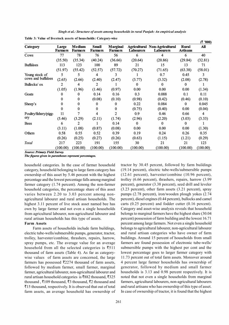
261
Singh et al.: Structure of assets among households in rural Punjab: An empirical analysis
Table 3: Value of livestock assets of households: Category-wise(` '000)
Category LargeFarmers
MediumFarmers
SmallFarmers
MarginalFarmers
AgriculturalLabourers
Non-AgriculturalLabourers
RuralArtisans
All
Cows 77 78 76 56 6 4 6 40(35.50) (35.34) (40.24) (36.66) (20.64) (20.86) (29.84) (32.81)
Buffaloes 113 123 100 89 21 15 13 71(51.97) (55.42) (52.57) (57.72) (70.27) (71.65) (63.38) (58.01)
Young stock ofcows and buffaloes
5 5 4 3 1 0.7 0.45 3(2.65) (2.66) (2.40) (2.47) (3.77) (3.32) (2.08) (2.78)
Bullocks/ ox 2 4 2 1 0 0 0 1(1.05) (1.96) (1.46) (0.97) 0.00 0.00 0.00 (1.34)
Goats 0 0 0.14 0.16 0.3 0.088 0.1 0.110 0 (0.08) (0.10) (0.98) (0.42) (0.46) (0.10)
Sheep’s 0 0 0 0 0.22 0.084 0 0.0450 0 0 0 (0.75) (0.40) 0.00 (0.04)
Poultry/fishery/pigg-ery
11 7 4 2 0.9 0.46 0.66 4(5.46) (3.29) (2.11) (1.74) (2.96) (2.20) (3.03) (3.33)
Bees 6 2 1 0.14 0 0 0 1(3.11) (1.08) (0.87) (0.08) 0.00 0.00 0.00 (1.30)
Others 0.58 0.55 0.52 0.39 0.19 0.24 0.26 0.35(0.26) (0.25) (0.27) (0.26) (0.63) (1.15) (1.21) (0.29)
Total 217 223 191 155 30 21 21 123(100.00) (100.00) (100.00) (100.00) (100.00) (100.00) (100.00) (100.00)
Source: Primary Field Survey.The figures given in parentheses represent percentages.
household categories. In the case of farmer householdcategory, household belonging to large farm category hasownership of this asset by 5.46 percent with the highestpercentage and the lowest percentage falls among marginalfarmer category (1.74 percent). Among the non-farmerhousehold categories, the percentage share of this assetvaries between 2.20 to 3.03 percent among non-agricultural labourer and rural artisan households. Thehighest 3.11 percent of live stock asset named bee hasown by large farmer and not even a single householdsfrom agricultural labourer, non-agricultural labourer andrural artisan households has this type of assets.Farm Assets
Farm assets of households include farm buildings,electric tube-wells/submersible pumps, generator, tractor,trolley, harvester/combine, thrashers, repairs, harrow,spray pumps, etc. The average value for an averagehousehold from all the selected categories is `511thousand of farm assets (Table 4). As far as category-wise values of farm assets are concerned, the largefarmers has possessed `2274 thousand of farm assets,followed by medium farmer, small farmer, marginalfarmer, agricultural labourer, non-agricultural labourer andrural artisan household categories is `882 thousand, `325thousand , `109 thousand, `3 thousand, `2 thousand and`15 thousand, respectively. It is observed that out of totalfarm assets, an average household has ownership of
tractor by 30.45 percent, followed by farm buildings(19.14 percent), electric tube-wells/submersible pumps(12.61 percent), harvester/combine (10.96 percent),trolley (6.66 percent), thrashers, repairs, harrow (3.99percent), generator (3.38 percent), seed drill and leveler(3.23 percent), other farm assets (3.21 percent), spraypumps (2.78 percent), iron/wooden plough yokes (2.74percent), diesel engines (0.44 percent), bullocks and camelcarts (0.25 percent) and fodder cutter (0.16 percent).Category and asset-wise analysis reveals that householdbelongs to marginal farmers have the highest share (30.04percent) possession of farm building and the lowest 16.71percent among large farmers. Not even a single householdbelongs to agricultural labourer, non-agricultural labourerand rural artisan categories who have owner of farmbuildings. Around 15 percent of households from smallfarmers are found possession of electronic tube-wells/submersible pumps with the highest per cent and thelowest percentage goes to larger farmer category with11.73 percent out of total farm assets. Moreover around4 percent large farmer households has ownership ofgenerator, followed by medium and small farmerhouseholds is 3.13 and 0.98 percent respectively. It isnoted that not even a single households from marginalfarmers, agricultural labourers, non-agricultural labourersand rural artisans who has ownership of this type of asset.In case of ownership of tractor, it is found that the highest

262
Indian J Econ Dev 12 (2): 2016 (April-June)
Table 4: Value of farm assets of households: Category-wise(` '000)
Category LargeFarmers
MediumFarmers
SmallFarmers
MarginalFarmers
AgriculturalLabourers
Non-AgriculturalLabourers
RuralArtisans
All
Farm buildings 380 195 78 32 0 0 0 97(16.71) (22.20) (24.26) (30.04) 0.00 0.00 0.00 (19.14)
Electric tube-wells/submersiblepumps
266 120 48 13 0 0 0 64(11.73) (13.68) (14.90) (12.57) 0.00 0.00 0.00 (12.61)
Generator 92 27 3 0 0 0 0 17(4.08) (3.13) (0.98) 0.00 0.00 0.00 0.00 (3.38)
Tractor 725 244 104 22 0 0 10 155(31.90) (27.64) (32.12) (20.13) 0.00 0.00 (68.88) (30.45)
Trolley 146 52 26 8 0 0 3 34(6.44) (5.99) (8.24) (7.79) 0.00 0.00 (23.35) (6.66)
Threshers, reapers,harrow
88 36 13 5 0 0 0 20(3.89) (4.13) (4.12) (4.92) 0.00 0.00 0.00 (3.99)
Bullocks/camelcarts
0 0 0 5 2 1 0 10 0 0 (4.86) (67.45) (66.13) 0.00 (0.25)
Iron/wooden ploughyokes
57 25 11 4 0.10. 0 0 14(2.54) (2.84) (3.45) (3.71) (3.38) 0.00 0.00 (2.74)
Harvester/combine 314 79 7 2 0 0 0 56(13.84) (9.03) (2.38) (1.92) 0.00 0.00 0.00 (10.96)
Seed drill andleveler
62 32 8 2 0 0 0 16(2.73) (3.67) (2.64) (1.86) 0.00 0.00 0.00 (3.23)
Diesel engines 11 4 0 0 0 0 0 2(0.49) (0.53) 0.00 0.00 0.00 0.00 0.00 (0.44)
Fodder cutter 2 1 0.88 0.65 0.22 0.14 0.22 0.82(0.10) (0.17) (0.27) (0.60) (7.26) (6.20) (1.48) (0.16)
Spray pumps 74 29 3 2 0.11 0.1 0.21 14(3.26) (3.38) (1.14) (1.94) (3.60) (4.68) (1.41) (2.78)
Others 52 31 17 10 0.56 0.53 0.74 16(2.29) (3.61) (5.50) (9.66) (18.31) (22.99) (4.88) (3.21)
Total 2274 882 325 109 3 2 15 511(100.00) (100.00) (100.00) (100.00) (100.00) (100.00) (100.00) (100.00)
Source: Primary Field Survey.The figures given in parentheses represent percentages.
(68.88 percent) percentage prevailing among rural artisanhousehold category, while the lowest (20.13 percent) fallsamong marginal farmer household category. Thepercentage of ownership of thresher, repair and harrowvaries as 3.89 to 4.92 percent among all farmer householdcategories. It is further found that 13.84 percent ofharvester/ combine possessed by large farm category withthe highest percentage, while the lower 1.92 percent goesto marginal farm category. Seed drill and leveler iscommonly found among all the farm-size categories inrural Punjab. All the sampled household categories haveownership of fodder cutter and spray pumps. In the caseof other farm assets, the highest percentage comes fromnon-agricultural labourer household category with 22.99percent, while the lowest percentage comes from large
farmer household category (2.29 percent) out of totalfarm assets possessed by all household categories in ruralPunjab.Financial and Non-agricultural Land Assets
The information regarding possession of financialassets (both cash/deposits and ornaments) and non-agricultural land assets among the households belongingto different categories is given in Table 5. It has beenobserved that an average household has financial assetsof worth `232 thousand. Category-wise analysis revealsthat the households from large farmer category have ahigher average value of financial assets of worth `923thousand. The corresponding figures for medium farmer,small farmer, marginal farmer, rural artisan, non-agricultural labourer and agricultural labourer household

263
categories are `501, `140, `89, `0.78, `0.71, and `0.64thousand respectively in descending order. The averagevalue of non-agricultural land has been found higheramong larger farmers of worth `112 thousand, followedby medium farmer (`39 thousand), small farmer (`15thousand), marginal farmer (`5 thousand), rural artisan(`0.49 thousand), non-agricultural labourer (`0.46thousand) and agricultural labourer (`0.39 thousand).CONCLUSIONS
The analysis reveals that among the sampledhouseholds, the value of durable assets is the highest,followed by those of farm assets, financial assets,livestock assets and non-agricultural land in that order.As far as category-wise ownership of different assetholdings is concerned, it has been observed that there isdirect relationship between farm-size and possession ofdifferent household assets in absolute terms among thefarmer household categories. But in relative terms, thereis an inverse relationship between farm-size and holdingof durable as well as livestock assets. The value of durableassets is the highest among the rural artisan householdcategory as compared to other non-farming householdcategories. There is direct relationship between havingdifferent farm assets and the farm-size among all farmerhousehold categories. The holding of farm assets increasedas farm-size increased and vice-versa in both absoluteand relative terms. Among the households belonging tonon-farming categories, the value of farm assets is thehighest among rural artisan household category. It isinteresting to note that in relative terms, the averagehousehold from medium farmer category has the highestshare of financial assets as a proportion out of total assets,followed by large farmer, marginal farmer, non-agricultural labourer, rural artisan and agricultural labourerhousehold categories. Wherever in absolute terms, it ishigher among large farmer household category, followedby medium farmer, small farmer, marginal farmer, ruralartisan, non-agricultural labourer and agricultural labourerhousehold categories. In the case of holding of non-
agricultural land and other assets, the highest share asexpected is of large farmer household category ascompare to other sampled household categories.REFERENCESAnonymous. 2011. Government of India. Economic survey
of India, Various Issues, Oxford University Press, NewDelhi.
Anonymous. 2013. Key indicators in debt and investmentin India. All India debt and investment survey. Ministryof Statistics and Programme Implementation,Government of India, New Delhi.
Anonymous. 2014. Government of Punjab. Statisticalabstract of Punjab, Various Issues, Economic Adviser,Government of Punjab, Chandigarh.
Bardhan, P. 1970. Green Revolution and agricultural labourers.Economic and Political Weekly. 5 (29, 30 & 31): 1239-1246.
Geetanjali, K and Rao, E.N. 2011. Poverty among weaver:Study of Srikakulam district in A.P. Southern Economist,44 (10): 21-24.
Jodhka, S.S. 1995. Who borrow? Who lends? : Changingstructure of informal credit in rural Haryana, Economicand Political Weekly. 30 (39): A123-A132.
Kaur, R. and Singh, G. 2010. Magnitude and correlates ofagriculture indebtedness in Punjab. Punjab Geographer,6: 51-60.
Nadkarni, M.V. 1988. Crisis of increasing costs in agriculture:Is there way out? Economic and Political Weekly. 23(39): A114-A119.
Rangi, P.S. and Sidhu, M.S. 1998. Growth of Punjabagriculture and sustainable development. 2. EcologicalSociety, Ludhiana and Centre for Research in Rural andIndustrial Development, Chandigarh.
Sangha, K.K. 2014. Modern agricultural practices and analysisof socio-economic and ecological impacts ofdevelopment in agriculture sector in Punjab: A review,Indian Journal of Agricultural Research. 48 (5): 331-341.
Shergill, H.S. 1998. Rural credit and indebtedness in Punjab.Monograph Series 4:1. Institute for Development andCommunications. Chandigarh, .
Table 5: Values of financial and non-agricultural land among households: Category-wise(` '000)
Category Cash and deposits Ornaments Total financial assets Non-agricultural landLarge farmers 167 756 923 112Medium farmers 57 444 501 393Small farmers 15 125 140 15Marginal farmers 9 80 89 5Agricultural labourers 0.35 0.29 0.64 0.39Non-agriculturallabourers
0.38 0.33 0.71 0.46
Rural artisans 0.42 0.36 0.78 0.49All 34 198 232 24Source: Primary Field Survey.

264
Indian J Econ Dev 12 (2): 2016 (April-June)
Shergill, H.S. 2010. Growth of farm debt in Punjab: 1997-2008. Institute for Development and Communications,Chandigarh.
Sidhu, H.S. 2005. Production condition on contemporaryPunjab. Journal of Punjab Studies. 12 (2):197-217.
Singh, P. and Tiwana, B.S. 2015. Rise in Capitalism in Punjab’sAgriculture: An Enquiry into the Mode of Production.In: Singh, G. Tiwana, B.S., Anupama, and Singh, S.
(ed.), Agricultural Performance and Rural Developmentin India, Publication Bureau, Punjabi University, Patiala.
Singh, S. 2000. Crisis in Punjab agricultural. Economic andPolitical Weekly. 35 (4): 1889-1892.
Zedong, Mao. 2011. How to differentiate classes in ruralareas. In: Patniak, U. (ed.), The agrarian questions inMarx and his successors. 2. Left World, Publication,New Delhi.

265
www.soed.in
Agricultural Resource and Income Inequality in NorthernRajasthanMada Melkamu* and N.K Singh
Department of Agricultural Economics, College of Agriculture, S.K Rajasthan Agricultural University, Bikaner
*Corresponding author’s email: [email protected]
Received: September 29, 2015 Accepted: April 15, 2016
Indian Journal of Economics and DevelopmentVolume 12 (2): 265-272
April-June, 2016DOI: 10.5958/2322-0430.2016.00135.9
ABSTRACTThe present study attempts to analyze resource and income inequality in Northern Rajasthan. The study used primarydata from 300 households following multistage random sampling process in the study area. To address resource andincome inequality, the study used Lorenz curve, Gini coefficients and dividing the sampled households into fifths (quintiles)approach. The study found Gini-coefficient value (0.499) for agricultural land, (0.476) for livestock holding (0.67) forirrigated land and (0.425) for income distribution, that indicates existence of high inequality among sampled householdsin Northern Rajasthan. Quintiles division analysis result also agrees with the Lorenz curve and Gini coefficients result.The uppermost 20 percent land holding is 2.5 times more than the assumed equal distribution rate, more than 102 timesmore than lowest 20 quintiles and more than six times the lowest 40 percent quintiles. The uppermost 20 percent quintileslivestock holding is more than 86 times higher than the lowest 20 percent quintiles and more than 2 times the expectedequal distribution amount. Surprisingly, uppermost 20 percent quintiles irrigated land holding is almost 8 times higherthan the lowest 60 percent quintiles and more than 3 times greater than the assumed equal distribution rate. All the dataresult indicates irrigated land is controlled by few people in Northern Rajasthan. The upper 20 percent quintiles incomeshare is more than two times higher than equal distribution and more than ten times higher than lowest 20 percent share.However, as compared to other inequality indicators, there is lower degree of income inequality. The Lorenz curveposition from equal distribution coincide with Gini coefficient results and quintiles division analysis results.
KeywordsAgricultural resource, Inequality, Income, poverty, Lorenz curve, Gini-coefficients, Rajasthan, India
JEL CodesD31, D63, I32, Q15
INTRODUCTIONAmong the most important economic challenges
facing India, the increases in the inequality of economicoutcomes needs attention like poverty. Growth alone isnot sufficient for poverty reduction-growth associatedwith progressive distributional changes will have a greaterimpact on poverty than growth that leaves distributionunchanged (Ames et al., 2001). The experience ofcountries that have succeeded in reducing povertysignificantly point to the important role of high rates ofeconomic growth combined with high rates ofemployment growth. High rates of economic growth ontheir own are insufficient to guarantee that povertyreduction will occur unless the benefits of economicgrowth are more equitably distributed. In the developing
world the main concern was focused on the relationshipbetween economic growth and income distribution, sincemany countries that had experienced growth rates abovetheir historical standard realized that such growth seemedto have negatively affected the income distribution, leadinginequality and failure to eliminate, even reduce, the levelof poverty (Todaro,1994)
Experience show that, absolute poverty can bealleviated if at least two conditions are met, first, economicgrowth occurs-or the mean income rises-on a sustainedbasis. Second, economic growth is either neutral to incomedistribution or reduces income inequality, poverty cannotbe reduced if economic growth does not occur; povertytends to change in the same direction as the mean income(Bruno et al., 1998). There are also good theoretical

266
Indian J Econ Dev 12 (2): 2016 (April-June)
reasons and empirical evidence to suggest that largeincome inequality is not good for either poverty reductionor economic growth, high levels of inequality contributeto high levels of poverty in several ways and initialdistribution of income (and wealth) can greatly affectthe prospects for growth and alleviation of mass poverty.In countries with high initial inequality, the poor tend tohave a lower share of the gains from growth. Economicinequality is major risk to poverty alleviation in its trend.
The report by Anonymous (2011) for India reiteratesthe growing divide. In 1994, the top 10 percent of India’spopulation and the bottom 40 percent controlled the sameportion of India’s wealth-around 25 percent. By 2010,India’s top 10 percent controlled nearly 30 percent ofIndia’s assets, and the share of the lower 40 percentdeclined to 21 percent. In addition, widely varying returnsto India’s very unequally distributed human capital areundoubtedly putting upward pressure on inequality. Poorhuman development attainments linked to povertycontribute to an inequitable growth process and losteconomic opportunities for India’s poor.
According to Anonymous (2015), rapid growth hasnot transformed the labour market and employmentconditions in the country. Employment grew merely by0.5 percent per annum from 2004-05 to 2011-12 - theperiod that saw the highest growth of GDP by 8.5 percentper annum. At the same time, 92 percent of workers arestill engaged in informal employment. Close to 276 millionworkers live below a poverty line of $2 per day, and theirbargaining positions have declined despite economygrowth. Further, both rural–urban disparities as well asinequality within urban areas in per capita expenditureare growing. Recent data also indicate a growingconcentration of per capita incomes at the top during thepost-reform period. As the distribution of incomes andexpenditures has become more unequal, poor people havenot gained sufficiently from rapid economic growth. MostEconomic Model postulates that resource inequalityaffects poverty by first.
Lack of assets is an effect as well as a cause ofpoverty in terms of income opportunities, consumptionand capability-building of people and their own institutions.The term ‘asset poverty’ indicates a vicious circle. Peoplewithout assets tend to be consumption-poor because theyrely mainly on selling their labour in poorly paid marketsor to the landed class, have nothing to sell or mortgage inhard times, and are economically dependent and politicallyweak. Land is the fundamental means of production inan agrarian society without which no agriculturalproduction can take place. An understanding of the patternof operational holdings distribution of land among statesis, therefore, of central importance to assist the process
of planning and targeting of poverty reduction. Well-targeted policies can reduce poverty by increasing theopportunities for poor people to gain and maintain secureaccess to productive assets, especially land, water andother natural resources, together with social assets suchas extension services, education and basic health care.Improving the assets of the rural poor has multiplier effectson the rate of economic growth.
Traditionally, governments have addressed thepoverty problem by implementing poverty-alleviationprograms through social safety nets that are intended toprovide some temporary relief for the poor. However, itis now well established that these programs at best providetemporary support, but they do not attack the causes ofpoverty. Poverty-alleviation programs are focused on the“consequences” of poverty rather than on its causes. Thistype of schemes provides benefits for rather short periodsof time, but leaves the poor in the same (or very similar)position when they are discontinued. Rural poverty is aproblem caused mainly by high inequality in resource.The ‘excess poverty’ present in many developingcountries is to be explained by the high level of inequality.This is in turn likely to be linked to high levels of inequalityin income generating assets (Attanazioand Székely, 1999). Therefore, to understand what causesincome inequality that we observe, we must firstdetermine how the distribution of income generating assetsis so unequal. This study was designed to assess howincomes generating agricultural assets are distributedamong households in Northern Rajasthan.METHODOLOGYSampling Technique
Multistage stratified random sampling procedurewas adopted for the selection of 300 sampled respondentsfrom Northern Rajasthan. Northern part of Rajasthanwas purposively selected for this study because ofRajasthan is one of the states where state-level HDIs(Human Development Indexes) are very low and thestate has given its 18th rank in poverty status among allthe states of India indicates poverty problem availabilitywhich needs further study. In the second stage, out ofseven districts, giving equal chance for each district, threedistricts namely Bikaner, Sri Ganga Negar and Nagaurwere selected. In the third stage, two tehsils from eachselected district were selected randomly. Namely: inBikaner district, Bikaner and Lunkaransar whereas in SriGanga Negar, Sadulshahar and Sri Ganganagar further inNagaur, Merta and Khinwsar tehsils were selectedrandomly. In the fourth stage, three villages from eachselected tehsil were selected randomly. Thus, totallyeighteen villages from six selected tehsils were selectedfor further selection of households. In the fifth stage, list
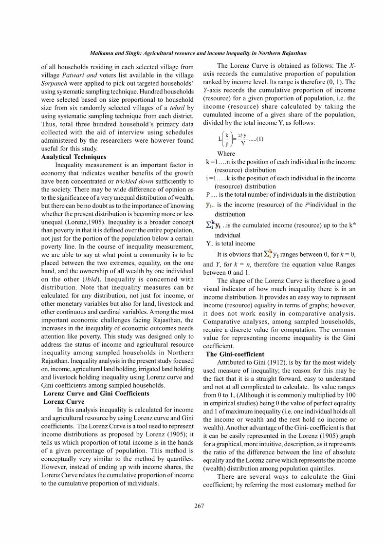
267
Malkamu and Singh: Agricultural resource and income inequality in Northern Rajasthan
of all households residing in each selected village fromvillage Patwari and voters list available in the villageSarpanch were applied to pick out targeted households’using systematic sampling technique. Hundred householdswere selected based on size proportional to householdsize from six randomly selected villages of a tehsil byusing systematic sampling technique from each district.Thus, total three hundred household’s primary datacollected with the aid of interview using schedulesadministered by the researchers were however founduseful for this study.Analytical Techniques
Inequality measurement is an important factor ineconomy that indicates weather benefits of the growthhave been concentrated or trickled down sufficiently tothe society. There may be wide difference of opinion asto the significance of a very unequal distribution of wealth,but there can be no doubt as to the importance of knowingwhether the present distribution is becoming more or lessunequal (Lorenz,1905). Inequality is a broader conceptthan poverty in that it is defined over the entire population,not just for the portion of the population below a certainpoverty line. In the course of inequality measurement,we are able to say at what point a community is to beplaced between the two extremes, equality, on the onehand, and the ownership of all wealth by one individualon the other (ibid). Inequality is concerned withdistribution. Note that inequality measures can becalculated for any distribution, not just for income, orother monetary variables but also for land, livestock andother continuous and cardinal variables. Among the mostimportant economic challenges facing Rajasthan, theincreases in the inequality of economic outcomes needsattention like poverty. This study was designed only toaddress the status of income and agricultural resourceinequality among sampled households in NorthernRajasthan. Inequality analysis in the present study focusedon, income, agricultural land holding, irrigated land holdingand livestock holding inequality using Lorenz curve andGini coefficients among sampled households. Lorenz Curve and Gini Coefficients Lorenz Curve
In this analysis inequality is calculated for incomeand agricultural resource by using Lorenz curve and Ginicoefficients. The Lorenz Curve is a tool used to representincome distributions as proposed by Lorenz (1905); ittells us which proportion of total income is in the handsof a given percentage of population. This method isconceptually very similar to the method by quantiles.However, instead of ending up with income shares, theLorenz Curve relates the cumulative proportion of incometo the cumulative proportion of individuals.
The Lorenz Curve is obtained as follows: The X-axis records the cumulative proportion of populationranked by income level. Its range is therefore (0, 1). TheY-axis records the cumulative proportion of income(resource) for a given proportion of population, i.e. theincome (resource) share calculated by taking thecumulated income of a given share of the population,divided by the total income Y, as follows:
.....(1)Yy
pkL
ki i
Wherek =1….n is the position of each individual in the income
(resource) distributioni =1…..k is the position of each individual in the income
(resource) distributionP…. is the total number of individuals in the distribution
.. is the income (resource) of the ithindividual in thedistribution
..is the cumulated income (resource) up to the kth
individualY.. is total income
It is obvious that ranges between 0, for k = 0,and Y, for k = n, therefore the equation value Rangesbetween 0 and 1.
The shape of the Lorenz Curve is therefore a goodvisual indicator of how much inequality there is in anincome distribution. It provides an easy way to representincome (resource) equality in terms of graphs; however,it does not work easily in comparative analysis.Comparative analyses, among sampled households,require a discrete value for computation. The commonvalue for representing income inequality is the Ginicoefficient. The Gini-coefficient
Attributed to Gini (1912), is by far the most widelyused measure of inequality; the reason for this may bethe fact that it is a straight forward, easy to understandand not at all complicated to calculate. Its value rangesfrom 0 to 1, (Although it is commonly multiplied by 100in empirical studies) being 0 the value of perfect equalityand 1 of maximum inequality (i.e. one individual holds allthe income or wealth and the rest hold no income orwealth). Another advantage of the Gini- coefficient is thatit can be easily represented in the Lorenz (1905) graphfor a graphical, more intuitive, description, as it representsthe ratio of the difference between the line of absoluteequality and the Lorenz curve which represents the income(wealth) distribution among population quintiles.
There are several ways to calculate the Ginicoefficient; by referring the most customary method for

268
Indian J Econ Dev 12 (2): 2016 (April-June)
calculating the Gini coefficient based on the Lorenz curve.Graphically, the Gini coefficient can be easily representedby the area between the Lorenz curve and the line ofequality. If income is distributed completely equally, thenthe Lorenz curve and the line of total equality are mergedand the Gini coefficient is zero. If one individual receivesall the income, the Lorenz curve would pass through thepoints (0,0), (100,0) and (100,100), and the surfaces Aand B would be similar, leading to a value of one for theGini-Coefficient.RESULTS AND DISCUSSION
Inequality is concerned with distribution. The overalllevel of inequality in a country, region or population group-and more generally the distribution of income, resourceor other attributes – is also in itself an important dimensionof welfare in that group. Inequality measures can becalculated for any distribution-not just for income orother monetary variables, but also for land, livestock andother continuous and cardinal variables (Anonymous,2011).
However, in the present study, inequality is calculatedfor agricultural resource and total family income byusing Lorenz curve and Gini coefficients. In addition tothese, the study utilized simplest way to measure inequalityby dividing the sampled households into fifths (quintiles)from poorest to richest, and reporting the levels orproportions of income (resource) that accrue to eachlevel using descriptive analysis. First the study investigatedthe status of agricultural resource inequality amongsampled households in Northern Rajasthan. Agriculturalresource inequality analysis focused on agricultural landholding, irrigated land holding and livestock holding usingLorenz curve and Gini Coefficients. Then, it assessestotal income inequality among sampled households in thestudy area. The pattern of resource distribution amongthe surveyed households of Northern Rajasthan iscalculated and results are reported in Table 1.
The perusal of Table 1 shows agricultural landdistributions among surveyed households in NorthernRajasthan. Land is the fundamental means of production
Table 1: Agricultural land distribution among surveyed households in Northern RajasthanAgricultural land (quintiles) Households
(No.)Cumulative
frequency ofhouseholds (%)
Totalagricultural
land (ha)
Share of totalagricultural land
(%)
Per householdagricultural land
(ha)Lowest 20 percent 60 20 8.5 0.49 0.142Low-mid 20 percent 60 40 123.75 7.10 2.063Middle 20 percent 60 60 273.1 15.67 4.55Mid-upper 20 percent 60 80 465.15 26.69 7.75Upper 20 percent 60 100 871.9 50.05 14.53Overall 300 - 1742.4 100 5.81Source: Authors' computations, based on household Survey Data, 2015
in an agrarian society without which no agriculturalproduction can take place. An understanding of the patternof operational holdings distribution of land among statesis, therefore, of central importance to assist the processof planning and targeting of poverty reduction. Upper20 percent land holders take the lion share and owned50.05 percent of total agricultural land whiles the lowest20 percent sampled household share is less than onepercent. Majority middle 60 percent household owned49.46 percent of total agricultural land. If each individualhad the same agricultural land holding in NorthernRajasthan, a household in each quintile can averagelyowned 5.81 hectare.
Conversely, a household from upper 20 percentowned 14.53 hectare but household from lowest 20percent owned only 0.142 hectare agricultural land. Theuppermost 20 percent land holding is 2.5 times more thanthe assumed equal distribution rate, more than 102 timesmore than lowest 20 quintiles and more than six timesthe lowest 40 percent quintiles. All these shows thepotential agricultural resource, land is unequallydistributed among sampled households in NorthernRajasthan. The Gini-coefficient value (0.499) obtainedfrom the data shows existence of unequal distribution ofagricultural land among sampled households (Table 5).This means few households hold major agricultural landand the rest households hold little agricultural land. Thisresult coincides with Melkamu and Bannor (2015), whofound and concluded Gini coefficient (0.6) value and theshape of the Lorenz curve shows existence of skeweddistribution of land holding and only five states hold morethan 50 percent of operational holdings of the country.Livestock Distribution among Surveyed Households
Livestock is capital assets produced in the past andcontributing to future product output. In India livestockis the source of food, income, employment and foreignexchange hence has potential key role in reducing ruralpoverty. For low income producers, livestock can serveas a store of wealth; provide draught power and organicfertilizer for crop production. Livestock sector in its bid

269
to help rural poor recently introduced technology whichis applicable for landless households.
This land-saving technology is alternative solutionfor household income poverty alleviation. Thereforeunderstanding of the pattern of operational holdingsdistribution of livestock among sampled households iscentral importance to assist the process of planning andtargeting of poverty reduction. Surveyed householdslivestock holding in TLU in Northern Rajasthan iscalculated and results are shown in Table 2.
Livestock distributions among surveyed householdsin Northern Rajasthan are depicted on Table 2. The resultsshow, the lowest 20 percent households owned just 0.56percent of total livestock holdings and highest 20 percenthouseholds owned 48.45 percent of total livestockholdings. The middle 60 percent households owned 50.99percent of total livestock holdings in Northern Rajasthan.If every household possessed equal number of livestockin TLU, a household in each quintile can averagely owned2.84 livestock in TLU. However, averagely eachhousehold from upper 20 percent possessed 6.9 livestockin TLU whereas each household from lowest 20 percentaveragely owned only 0.08 livestock in TLU. Theuppermost 20 percent quintiles livestock holding is morethan 86 times higher than the lowest 20 percent quintilesand more than 2 times the expected equal distributionamount. The livestock distribution results also indicatepresence of uneven distribution of livestock amongsampled households in Northern Rajasthan.
The Gini-coefficient (0.476) also supports existence
Table 2: Livestock distribution among surveyed households in Northern RajasthanLivestock (quintiles) Households
NumberPer Household Livestock
(TLU)Cumulative
frequency ofhouseholds (%)
Totallivestock in
(TLU)
Share of totallivestock (%)
Lowest 20 percent 60 20 4.94 0.56 0.08Low-mid 20 percent 60 40 75.93 8.91 1.30Middle 20 percent 60 60 142.43 16.72 2.40Mid-upper 20 percent 60 80 216.03 25.36 3.60Upper 20 percent 60 100 412.96 48.45 6.90Overall 300 852.29 100 2.84Source: Authors' computations, based on household survey data, 2015
of inequality in livestock holding among sampledhouseholds (Table 5). This result agrees with Melkamuand Bannor (2015), who found Gini coefficient (0.54)value for Indian livestock distribution among states andtheir Lorenz curve shape showed existence of skeweddistribution for livestock distribution. They finallyconclude that only five states owned more than 55 percentshare and the countries 90 percent livestock populationis accumulated only in 14 states.Irrigated Land Distribution among Households
Recently farm household income depends more onwater than land. Whereas land was the primary resourceaffecting agricultural production in the early decades ofthe twentieth century, access to irrigation has taken onincreasing importance in recent decades. Improved accessto irrigation infrastructure will increase crop yield,agricultural production and farm income within a region.The irrigated land distribution among households ofNorthern Rajasthan is presented in Table 3. According totable 3, lowest 20 percent and low-mid 20 percenthousehold’s do not owned any irrigated land. Upper 20percent owned more than 63 percent of total irrigatedland. The mid-40 percent owned 36.49 percent of totalirrigated land in Northern Rajasthan. If every householdowned equal irrigated land holding in Northern Rajasthan,a household in each quintile can averagely possessed 2.41hectare irrigated land. However, each household fromupper 20 percent in Northern Rajasthan averagely owned7.66 hectare irrigated land on the other hand householdfrom lowest 20 percent and low-mid 20 percent do not
Malkamu and Singh: Agricultural resource and income inequality in Northern Rajasthan
Table 3: Irrigated Land distribution among surveyed households in Northern RajasthanLivestock (quintiles) Households
(No.)Cumulative frequency
of households (%)Total irrigated
land (ha)Share of total
irrigated land (%)Per household
irrigated land (ha)Lowest 20 percent 60 20.00 - - -Low-mid 20 percent 60 40.00 - - -Middle 20 percent 60 60.00 59.50 8.22 0.99Mid-upper 20 percent 60 80.00 204.50 28.27 3.41Upper 20 percent 60 100.00 459.40 63.51 7.66Overall 300 - 723.40 100.00 2.41Source: Authors' computations, based on household survey data, 2015

270
Indian J Econ Dev 12 (2): 2016 (April-June)
owned any irrigated land.Surprisingly, uppermost 20 percent quintiles irrigated
land holding is almost 8 times higher than the lowest 60percent quintiles and more than 3 times greater than theassumed equal distribution rate. All the data result indicatesirrigated land is controlled by few people in NorthernRajasthan. To see the distribution of irrigated land amongsampled households graphically, Lorenz curve is drawnand depicted on figure 3.
Gini coefficient value (0.67) obtained from the datashows existence of skewed distribution of irrigated landamong sampled households (Table 5). This outcomeagrees with Melkamu and Bannor (2015), who foundalmost equal value of Gini coefficient (0.66) for irrigatedland distribution in India and showed existence of bigdifference in irrigation land distribution among states andconcluded that five states own more than 56 percent ofirrigated area of the country and more than 90 percent ofirrigated land found in only 11 states.Income Inequality
Total income is defined as household’s disposableincome in a particular year. It consists of farm or non-farm income or both. In this particular study, total incomeis sum of farm and non-farm income of a family memberin a particular year (March 2014 to April 2015). To starttotal income inequality analysis, the pattern of total incomedistribution among the surveyed households of NorthernRajasthan is calculated and results are reported in Table4.
The perusal of Table 4 shows income distributionsamong the surveyed households in Northern Rajasthan.The share of the lowest 20 percent households in incomewas 4.48 percent. The share of the middle 60 percenthouseholds accounted for 47.54 percent and uppermost20 percent households owned as much as 47.98 percentof the total income. If each individual had the sameincome in Northern Rajasthan, a household in each quintilepossessed `272,513 income annually. Conversely,averagely each household from upper 20 percentmaintained `653,759 income annually whereas ahousehold from lowest 20 percent maintained `61,055
income annually. The upper 20 percent share is morethan two times higher than equal distribution and morethan ten times higher than lowest 20 percent share. Theresult shows that in Northern Rajasthan, income is notequally distributed. However, as compared to otherinequality indicators, there is lower degree of incomeinequality.
Gin-coefficient value of 0.425 also approves theexistence of inequality in income distribution in the studyarea (Table 5). This outcome agrees with Melkamu andBannor (2015), who found and concluded existence ofper capital income inequality in India. They finallyconclude that, inequality in per capital income in thecountry is not serious like other resources inequality.
Table 4: Overall Gini-coefficient summaryParticulars Gini-CoefficientAgricultural land 0.499Irrigated land 0.670Livestock 0.476Income 0.425
CONCLUSIONSAND RECOMMENDATIONSUpper 20 percent land holders take the lion share
and owned 50.05 percent of total agricultural land whilesthe lowest 20 percent sampled household share is lessthan one percent. Majority middle 60 percent householdowned 49.46 percent of total agricultural land. If eachindividual had the same agricultural land holding inNorthern Rajasthan, a household in each quintile canaveragely owned 5.81 hectare. Conversely, a householdfrom upper 20 percent owned 14.53 hectare but householdfrom lowest 20 percent owned only 0.142 hectareagricultural land. The uppermost 20 percent land holdingis 2.5 times more than the assumed equal distributionrate, more than 102 times more than lowest 20 quintilesand more than six times the lowest 40 percent quintiles.All these shows the potential agricultural resource, landis unequally distributed among sampled households in
Table 4: Total Income distribution among surveyed households in Northern RajasthanIncome quintiles Households
NumberCumulative frequency
of householdsTotal income
(`)Share of total
income (percent)Income per
household (`)Lowest 20 percent 60 20 3,663,280 4.48 61,055Low-mid 20 percent 60 40 8,399,080 10.27 139,985Middle 20 percent 60 60 12,660,631 15.49 211,011Mid-upper 20 percent 60 80 17,805,221 21.78 296,754Upper 20 percent 60 100 39,225,576 47.98 653,759Overall 300 81,753,788 100 272,513Source: Authors' computations, based on household survey data, 2015

271
Northern Rajasthan. The Lorenz curve locus foragricultural land holding shows, existence of skeweddistribution among sampled households. Gini-coefficientvalue (0.499) obtained from the data shows existence ofunequal distribution of agricultural land among sampledhouseholds. This means few households hold majoragricultural land and the rest households hold littleagricultural land.
The lowest 20 percent households owned just 0.56percent of total livestock holdings and highest 20 percenthouseholds owned 48.45 percent of total livestockholdings. The middle 60 percent households owned 50.99percent of total livestock holdings in Northern Rajasthan.If every household possessed equal number of livestockin TLU, a household in each quintile can averagely owned2.84 livestock in TLU. However, averagely eachhousehold from upper 20 percent possessed 6.9 livestockin TLU whereas each household from lowest 20 percentaveragely owned only 0.08 livestock in TLU. Theuppermost 20 percent quintiles livestock holding is morethan 86 times higher than the lowest 20 percent quintilesand more than 2 times the expected equal distributionamount. The livestock distribution results also indicatepresence of uneven distribution of livestock amongsampled households in Northern Rajasthan. The curveshows the existence of inequality. The Gini-coefficient(0.476) also supports existence of inequality in livestockholding among sampled households.
Lowest 20 percent and low-mid 20 percenthousehold does not owned any irrigated land. Upper 20percent owned more than 63 percent of total irrigatedland. The mid-40 percent owned 36.49 percent of totalirrigated land in Northern Rajasthan. If every householdowned equal irrigated land holding in Northern Rajasthan,a household in each quintile can averagely possessed 2.41hectare irrigated land. However, each household fromupper 20 percent in Northern Rajasthan averagely owned7.66 hectare irrigated land on the other hand householdfrom lowest 20 percent and low-mid 20 percent do notowned any irrigated land. Surprisingly, uppermost 20percent quintiles irrigated land holding is almost 8 timeshigher than the lowest 60 percent quintiles and more than3 times greater than the assumed equal distribution rate.All the data result indicates irrigated land is controlled byfew people in Northern Rajasthan. The Lorenz curve locusmove far away from line of perfect equality in figure 3.It shows existence of unequal distribution of irrigatedland among sampled households. Gini coefficient value(0.67) obtained from the data shows existence of skeweddistribution of irrigated land among sampled households.
The share of the lowest 20 percent households inincome was 4.48 percent. The share of the middle 60percent households accounted for 47.54 percent and
uppermost 20 percent households owned as much as47.98 percent of the total income. If each individual hadthe same income in Northern Rajasthan, a household ineach quintile possessed `272,513 income annually.Conversely, averagely each household from upper 20percent maintained `653,759 income annually whereas ahousehold from lowest 20 percent maintained `61,055income annually. The upper 20 percent share is morethan two times higher than equal distribution and morethan ten times higher than lowest 20 percent share. Theresult shows that in Northern Rajasthan, income is notequally distributed. However, as compared to otherinequality indicators, there is lower degree of incomeinequality. The Lorenz curve drawn to see how totalincome is distributed among the surveyed households inNorthern Rajasthan shows the existence skeweddistribution. Gin-coefficient value of 0.425 also approvesthe existence of inequality in income distribution in thestudy area.
In sum, we have constructed a detailed profile andcorrelates of resource and income inequality based onthe household survey data of 300 households. Theevidence from empirical analysis suggests that irrigatedland and farm land inequality have highest Gin-coefficient.Income and livestock relatively diffused better than otherresource in Northern Rajasthan.
The policymakers need to focus on both reduceinequality and promote economic growth. Assessmentsof economic performance should not focus solely onoverall income growth, but also take into account incomedistribution. Policies that encourage education, well-designed and sustainable employment creation institutions,proper tax and transfer systems can all reduce incomeinequality.REFERENCESAmes, B., Brown, W., Devarajan, S., and Izquierdo, A. 2001.
Macroeconomic policy and poverty reduction .International Monetary Fund and the World Bank:Washington DC.
Anonymous. 2011. Perspectives on poverty in India, Stylizedfacts from survey data. World Bank, 1818 H Street NW,Washington, DC 20433, USA.
Anonymous. 2014. Working for the few. World EconomicForum and Oxford Committee for Famine Relief) briefingPaper 178 (2014). Culled from www.oxfam.org
Anonymous. 2015. Addressing economic inequality in India.International Centre for Human Development (IC4HD),National Institute of Advanced Studies (NIAS ) Campus,Bengaluru.
Attanazio, O and Szekely, M. 1999. An asset-based approachto the analysis of poverty in Latin America. ResearchNetwork, office of the Chief Economic, Working PaperNo. R-376, IADB,Washington.
Bruno, M., Martin, R., and Lyn, S. 1998. Equity and growth in
Malkamu and Singh: Agricultural resource and income inequality in Northern Rajasthan

272
Indian J Econ Dev 12 (2): 2016 (April-June)
developing countries: Old and new perspectives on thepolicy issues. In: Income distribution and high-qualitygrowth (ed) Tanzi, V. and Chu, K.Y., Cambridge, Mass:MIT Press.
Gini, C. 1912. Variability and mutability. C. Cuppini, Bologna,Reprinted in Memorie di metodologica statistica (Ed.Pizetti, E and Salvemini, T.). Libreria Eredi Virgilio Veschi,Rome.
Lorenz, M.O. 1905. Methods of measuring the concentration
of wealth. American Statistical Association. New Series,No 70.
Melkamu, M. and Bannor, R.K. 2015. Estimation ofagricultural resource inequality in India using Lorenzcurve and Gini coefficient approach. InternationalJournal of Current Research and Academic Review. 3(4): 174-184.
Todaro, M.1994. Economic development, Fifth edition, Longman Group. Harlow, United Kingdom.

273
Indian Journal of Economics and DevelopmentVolume 12 No.(2): 273-282
April-June, 2016DOI: 10.5958/2322-0430.2016.00136.0
www.soed.in
BSE SME Equity Financing Platform: A study of Index Risk-Return ParadoxAmanjot Singh* and Parneet Kaur
University School of Applied Management, Punjabi University, Patiala-147002 (India)
*Corresponding author’s email: [email protected]
Received: March 03, 2016 Accepted: May 25, 2016
ABSTRACTThe study attempts to introduce an innovative initiative of the BSE’s SME equity financing segment and explore the timevarying risk-return relationship of the BSE SME IPO index by employing GARCH-M, TGARCH-M, EGARCH-M andAsymmetric CGARCH models. The results spotlight the existence of a positive risk-return relationship between short runvolatility component and the actual returns, whereas a negative relationship has been observed between the long runvolatility and index returns. The results reported by the GARCH-M, EGARCH-M and TGARCH-M model in the context ofthe BSE SME IPO index shows insignificant, but a positive relationship between the risk and return. A positive shock hasa more pronounced impact on volatility in case of the BSE SME IPO segment. A study relating to the relationship betweenthe index risk and returns is an imperative task to be performed by the existing and prospective investors.
KeywordsExpected volatility, GARCH, IPO, long run volatility, small and medium enterprise, unexpected volatility
JEL CodesC10, C58, G12
INTRODUCTIONThe present pragmatic ‘Make in India’ campaign of
the Modi Government is not achievable withoutconsidering the contribution of the Micro, Small andMedium Enterprises (MSME hereafter). There is nodearth of availability of data in the context of MSME’scontribution to the Gross Domestic Product, exports,employment creation, industrial assistance to the largeenterprises and overall prosperity of the nation. Despitethe contribution of the MSME segment to the overalldevelopment of an economy, it is still wriggling out ofthe financing gap, particularly in developing economiescreated due to the higher cost of capital, higher collateralrequirements, lack of financial intermediaries, inefficientdebt and equity markets (Dalberg, 2011). Moreover, it isdifficult for these industries to finance through non-bankdebt sources due to small scale driven inbuilt fluctuationspresent in the cash flow generation processes. Theexposure of the SMEs toward the international flows
has further made the segment to consider the currencyfluctuation risks as well (Gopal and Jain, 2007). Anotheralternative yet not that popular is raising funds throughthe equity market platform. A reason that could beattributed to the difficulties in the equity model of raisingfunds can be the availability of a separate segment, riskpremium expected by the investors, informationasymmetry, lower governance standards and listingrequirements. The very small and riskier nature of theindustries makes the sector to witness a financing gap,thereby having an impact on their working capital andfixed asset financing, technology levels and operatingefficiencies. Speaking overall, Bhattacharjee andChakrabarti (2013) highlighted risk aversive behavior ofthe banking sector that has led to a significant decline inthe availability of the loanable funds in the post liberalizationperiod for the Indian manufacturing sector. Even theofficial documents admitted subdued industrial growthas a result of lack of credit (Anonymous, 2013). The

274
Indian J Econ Dev 12 (2): 2016 (April-June)
term ‘MSME’ is taken differently across differentcountries keeping into view various criteria’s like thesales, number of employees employed, capital investedin the assets. In the context of Indian economy, thesegregation of the MSME sector is done on the basis ofcapital invested in the assets of the business. As per theprovisions of Micro, Small & Medium EnterprisesDevelopment (MSMED) Act (2006) the definition ofMicro, Small and Medium Enterprises (MSME) is basedon the nature of the industry i.e. a manufacturingenterprise or a service enterprise.
Chinese SME index. In this study, we will be focussingon the Small and Medium Enterprises’ trade platform onlybarring the Micro sector. The whole paper has beendivided into five sections. Section I introduces the studyto be undertaken, Section II reviews the SME financingpattern over a period of time, Section III highlights theBSE SME equity financing segment, Section IV estimatesthe time varying risk-return relationship of the BSE SMEIPO index and Chinese SME index and lastly Section Vconcludes the paper.II. SME Financing-A Review
In the present scenario, a first generationentrepreneur has so many alternatives to access seed aswell as developmental capital in India, but the equitysegment has not been fully exhausted by the industries.The various alternative options through which anentrepreneur can raise funds are securitisation of SMEcredit, factoring, accessing equity capital from SMEExchange, venture capital, cash flow based financing,etc. (Raj, 2012). The study also highlighted the fact thatabout 45.2 percent of the enterprises are being located inthe rural areas. The location of the industries in the ruralareas itself explain the probable low contribution of theinstitutional sources of funds towards the balance sheetof MSME sector. The emergence of the US financialcrisis in the year 2007-2009, have further exacerbatedthe financial clamour of these industries. Due to theadoption of quantitative easing policy by the US FederalReserve after the 2008 crisis, the circulation of ‘HotMoney’ or easy money has increased all over the world(Lim et al., 2014). As a result of this signalling effect anddamaged trade relations, the central bankers, especiallyin emerging markets like India increased the interest rates,reduced liquidity and adopted stringent restructuringprovisions, which further hampered the functioning andcontribution of the sector towards the economy.
According to RBI statistics, the contribution of thecommercial banks towards the medium sector hasremained more or less same all through the years from2007 to 2014, but the share of micro and small industrieshave increased over a period of time advocating theeffectiveness of priority sector lending policy of RBI forthe commercial banks. The bank borrowings act asprimary source of external financing for the small andmid cap segment, as indicated by Majumdar (2014).Anonymous (2012) in its report titled Micro, Small andMedium Enterprise Finance in India, advocated thesituation of MSME financing gap in India. As a matter offact, the total demand requirement was INR 32.5 trillion,out of which around INR 20 trillion is still considered asan institutional financial gap. The contribution of theimmediately addressable equity is far lesser in comparisonto the contribution of the debt sector, whereas in the
Table 1: Definition of MSMEs as per MSMED Act,2006Enterprises Investment in assetsMicro Less than `25 Lakh
Small More than `25 Lac but does not exceed`5 crores.
Medium More than `5 crores but does not exceed`10 crores
Table 1 reports the definition of MSM enterpriseskeeping in view the investments in plant & machinery.The turnover and the credit size of the industries alsoacts as another criteria of defining the MSM enterprisesby the financial institution (Anonymous , 2012). Thepresent study attempts to achieve three objectivestheoretically as well as empirically. The first objective isto review the Small and Medium enterprises’ access tofinance over a period of time. Secondly, to introduce thereaders with the SME exchange platform and an IPOindex of the Bombay Stock Exchange Ltd. Thirdly, wehave tried to capture time varying risk-return relationshipof the SME IPO index by employing GeneralisedAutoregressive Conditional Heteroskedastic in MeanModel [GARCH-M (1,1)], Threshold GARCH-M (1,1),Exponential GARCH-M (1,1) and especially AsymmetricComponent GARCH (1,1) model, making the study firstof its kind in all the perspectives. The SME exchangeplatform is an emerging platform introduced by theBombay Stock Exchange as an innovative initiative forthe small and medium enterprises garner funds from theinvestors. A study relating to the relationship between theindex returns and expected long run and short run volatilityfollowed by unexpected volatility is an imperative task tobe performed by the various financial institutions in theircapacity to invest in these companies. As the exchangeplatform is a secondary aspect of the capital market, itdoes provide information and signals with regard to therisk and return to the prospective companies as well asinvestors in the primary market. To make the thingscomparable with another emerging market, we alsoestimated the time varying risk-return relationship of the
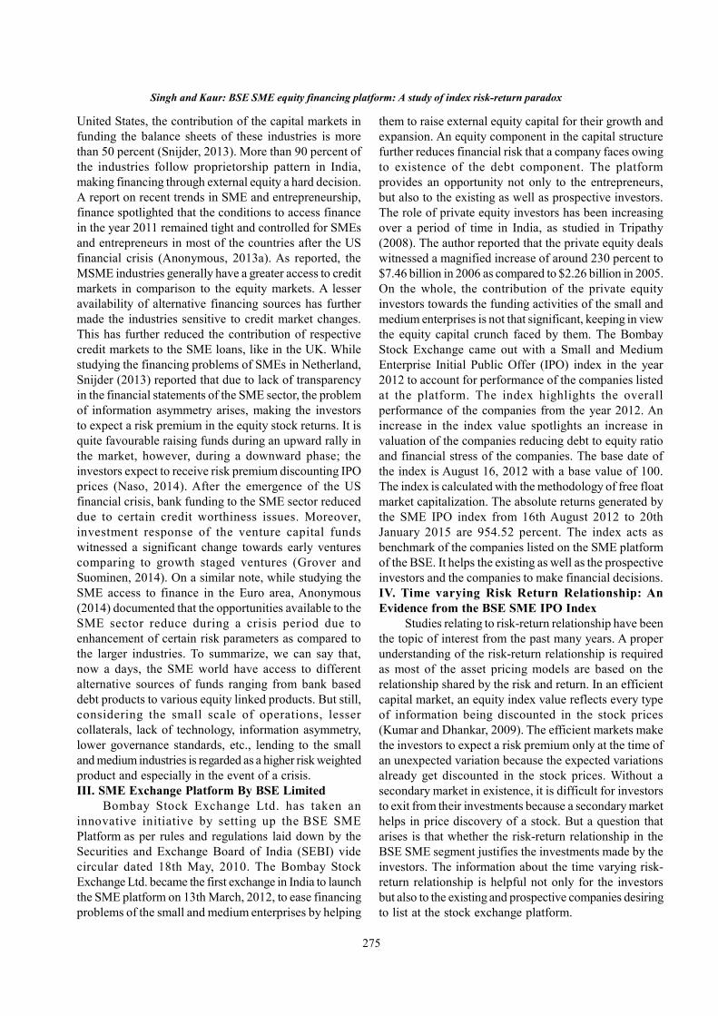
275
United States, the contribution of the capital markets infunding the balance sheets of these industries is morethan 50 percent (Snijder, 2013). More than 90 percent ofthe industries follow proprietorship pattern in India,making financing through external equity a hard decision.A report on recent trends in SME and entrepreneurship,finance spotlighted that the conditions to access financein the year 2011 remained tight and controlled for SMEsand entrepreneurs in most of the countries after the USfinancial crisis (Anonymous, 2013a). As reported, theMSME industries generally have a greater access to creditmarkets in comparison to the equity markets. A lesseravailability of alternative financing sources has furthermade the industries sensitive to credit market changes.This has further reduced the contribution of respectivecredit markets to the SME loans, like in the UK. Whilestudying the financing problems of SMEs in Netherland,Snijder (2013) reported that due to lack of transparencyin the financial statements of the SME sector, the problemof information asymmetry arises, making the investorsto expect a risk premium in the equity stock returns. It isquite favourable raising funds during an upward rally inthe market, however, during a downward phase; theinvestors expect to receive risk premium discounting IPOprices (Naso, 2014). After the emergence of the USfinancial crisis, bank funding to the SME sector reduceddue to certain credit worthiness issues. Moreover,investment response of the venture capital fundswitnessed a significant change towards early venturescomparing to growth staged ventures (Grover andSuominen, 2014). On a similar note, while studying theSME access to finance in the Euro area, Anonymous(2014) documented that the opportunities available to theSME sector reduce during a crisis period due toenhancement of certain risk parameters as compared tothe larger industries. To summarize, we can say that,now a days, the SME world have access to differentalternative sources of funds ranging from bank baseddebt products to various equity linked products. But still,considering the small scale of operations, lessercollaterals, lack of technology, information asymmetry,lower governance standards, etc., lending to the smalland medium industries is regarded as a higher risk weightedproduct and especially in the event of a crisis.III. SME Exchange Platform By BSE Limited
Bombay Stock Exchange Ltd. has taken aninnovative initiative by setting up the BSE SMEPlatform as per rules and regulations laid down by theSecurities and Exchange Board of India (SEBI) videcircular dated 18th May, 2010. The Bombay StockExchange Ltd. became the first exchange in India to launchthe SME platform on 13th March, 2012, to ease financingproblems of the small and medium enterprises by helping
them to raise external equity capital for their growth andexpansion. An equity component in the capital structurefurther reduces financial risk that a company faces owingto existence of the debt component. The platformprovides an opportunity not only to the entrepreneurs,but also to the existing as well as prospective investors.The role of private equity investors has been increasingover a period of time in India, as studied in Tripathy(2008). The author reported that the private equity dealswitnessed a magnified increase of around 230 percent to$7.46 billion in 2006 as compared to $2.26 billion in 2005.On the whole, the contribution of the private equityinvestors towards the funding activities of the small andmedium enterprises is not that significant, keeping in viewthe equity capital crunch faced by them. The BombayStock Exchange came out with a Small and MediumEnterprise Initial Public Offer (IPO) index in the year2012 to account for performance of the companies listedat the platform. The index highlights the overallperformance of the companies from the year 2012. Anincrease in the index value spotlights an increase invaluation of the companies reducing debt to equity ratioand financial stress of the companies. The base date ofthe index is August 16, 2012 with a base value of 100.The index is calculated with the methodology of free floatmarket capitalization. The absolute returns generated bythe SME IPO index from 16th August 2012 to 20thJanuary 2015 are 954.52 percent. The index acts asbenchmark of the companies listed on the SME platformof the BSE. It helps the existing as well as the prospectiveinvestors and the companies to make financial decisions.IV. Time varying Risk Return Relationship: AnEvidence from the BSE SME IPO Index
Studies relating to risk-return relationship have beenthe topic of interest from the past many years. A properunderstanding of the risk-return relationship is requiredas most of the asset pricing models are based on therelationship shared by the risk and return. In an efficientcapital market, an equity index value reflects every typeof information being discounted in the stock prices(Kumar and Dhankar, 2009). The efficient markets makethe investors to expect a risk premium only at the time ofan unexpected variation because the expected variationsalready get discounted in the stock prices. Without asecondary market in existence, it is difficult for investorsto exit from their investments because a secondary markethelps in price discovery of a stock. But a question thatarises is that whether the risk-return relationship in theBSE SME segment justifies the investments made by theinvestors. The information about the time varying risk-return relationship is helpful not only for the investorsbut also to the existing and prospective companies desiringto list at the stock exchange platform.
Singh and Kaur: BSE SME equity financing platform: A study of index risk-return paradox

276
Indian J Econ Dev 12 (2): 2016 (April-June)
The historical researchers concluded a linear positiverelationship between the expected returns and systematicrisk, i.e. the higher the risk higher the return to arrive ata price discovery model (Sharpe, 1964; Linter, 1965;Mossin, 1966). Extending this static linear relationship tothe dynamic framework, Merton (1973-1980) advocateda positive linear relationship between the conditionalexpected excess returns and time varying variance. Onthe other hand, Bowman (1980), Campbell (1987), Breenet al. (1989), and Whitelaw (1994) came out with thefindings of an inverse relationship between the risk andreturns. Badhani (2007) examined the said relationshipfrom three different angles: the effect of expected varianceon the expected returns, the effect of unexpected returnshocks on conditional variance and simultaneous regimeswitching relationship between the risk and return. Inthe present study, we have covered first and second aspectof the relationship with an additional focus on long andshort run risk-return relationship. The large number ofproblems faced by the SME sector has made the segmentquite riskier for an equity investor (Sharma, 2012). Theequity investors expect a risk premium for holding a riskierventure. Expected variations are regarded as expectedvolatility, whereas unexpected variations in the stockreturns are recognized as unexpected volatility.DATA
The daily data relating to the SME index have beencollected from the website of Bombay Stock Exchangeranging from, 16th August, 2012 to 20th January, 2015without adjusting for risk free rate of return. Althoughthe time period is small but sufficient enough to capturethe GARCH effects (Hwang & Pereira, 2006). To makea comparison with the Chinese market, Chinese SMEindex values have been gathered from the GOOGLEfinance database ranging from 6th March 2009 to 5thMay 2014 as per availability and without considering therisk free rate of return. A study can also be conducted bytaking respective stock prices of different companies listedat the platform to comprehend the risk return parameters.But here we are studying the overall SME market’s risk-return relationship. The daily continuously compoundingreturns are computed by taking natural log of the series.
( ) )1.......(100P-PLogR 1-ttt ×=Where Rt is the daily return, Pt is the current price
and Pt-1 is the previous day’s price. The returns arecalculated in the local currency terms.METHODOLOGY
The ICAPM (Intertemporal Capital Asset PricingModel) is generally employed to compute and explorethe said relationship, but, we have employed GARCH-M(1,1), EGARCH-M (1,1), TGARCH-M (1,1) andasymmetric CGARCH (1,1) model with ARMA (1,1) as
the ‘mean’ equation model. Generally, the markets areappeared to be inefficient because of the presence ofautocorrelation in the returns thereby making the seriesto witness heteroskedasticity in the error terms, wherebythe investors can earn abnormal returns. A very simplisticapproach to measure risk can be standard deviation ofthe past returns, but the historical estimates are not robustin comparison to other volatility modelling methods likeGARCH (Akgiray, 1989). The plain vanilla GARCH (1,1)model has been developed by Bollerslev (1986), whereina conditional variance is a function of past error termsand past conditional variances. The conditional variancesgenerated from a GARCH based model act as proxy oftime varying risk. To apply the GARCH type models, theresidual variances derived from the ‘mean’ equation shouldbe heterogeneous that is, changing over a period of time.The plain vanilla model has been further extended tovarious other GARCH type models, like EGARCH(Nelson, 1991), TGARCH (Glosten et al., 1993),CGARCH, PGARCH, etc.GARCH-M Model
The GARCH-M model with a variance parameter inthe ‘mean’ equation helps in analyzing the impact ofconditional variance on the expected returns. The meanequation, which is same for all the models employedexcept CGARCH (1,1) model, has been defined as follows:
)2.......(εhγqepRcR tt1-t1-tt ++++=
Where is the constant term, and are therespective coefficients of the Autoregressive (AR) andMoving average (MA) terms and is the error termwith mean zero and independently distributed. Parameter
in the mean equation measures the intertemporal impactof risk on the expected returns. The autoregressive partexplains contribution of the one day past return in theestimation of the current conditional return. On a similarnote, moving average explains the impact of one day pastnews on the current conditional return.
)3.......(hβεααh 1-t12
1-t10t ++=
1 and 1 capture the news impact on the conditionalvariance and the persistency in volatility respectively. Thetotal of 1 and should be less than one to make theresults stationary. The parameters of the GARCH modelshave been estimated by assuming normal distribution ofthe error terms and maximum likelihood approach.EGARCH-M Model
Another model which has been employed to accountfor leverage effect is the EGARCH model, which furthertakes into account logged variance to ensure positivity inthe conditional variances. The model has been developedby Nelson (1991).

277
)4.......(εhγqepRcR tt1-t1-tt ++++=
)5(.....2log 1-11-
1-
1-
1-21 t
t
t
t
tt h
hhh
Where is an asymmetric coefficient. Againconditional variance has been included in the ‘mean’equation to check for volatility feedback. The leverageeffect will be there when <0 and found to be significant.TGARCH-M Model
The TGARCH model, also known as GJR modelanalyses the impact of a negative shock on the volatilityor in short the ‘leverage effect’ (Black, 1976; Christie,1982). A leverage effect further entails to increasedexpected returns, thereby signifying a positive relationshipbetween volatility and the expected returns terming it asvolatility feedback hypothesis (French et al., 1987). Themodel is specified as:
)6.......(111-21-
21-10 tttttt hDh
Where, Dt-1 is a dummy variable to ascertain theleverage effect of a negative shock (Kaur and Singh,2015). If t-1<0 then the value 1 is assigned and otherwisezero. If is found to be significant and positive, then anegative shock has a leverage impact on the conditionalvariance ( ) as compared to the positive one. 1 and1capture the news impact on the conditional varianceand the persistency in volatility respectively. is aconditional variance parameter entered into the ‘mean’equation to capture volatility feedback. The non-negativityconstraints are o > 0, > 0, > 0, and > 0.CGARCH-M Model
The CGARCH model was introduced by Ding et al.(1993), which demarcates the volatility into twocomponents, long run and short run. Alom et al. (2012)employed CGARCH model to model food price volatilityand analysed the long run component and its spilloverimpacts. Similarly, to estimate the volatilities and spillovereffects between developed and emerging marketeconomies, Kharchenko and Tsvetkov (2013) usedCGARCH model. In the component GARCH (CGARCH)model, the constant conditional variance condition ofGARCH (1, 1) model is replaced with a time varyingcomponent ‘q’ to account for long-run volatility. Firstly,a ‘mean’ equation is defined, wherein the derived residualsare factored into the variance equation to captureconditional variances. To separately model the relationshipbetween the long run and short run risk component, theconditional variance term has not been included in themean equation.
)7.......(εeβRββR t1-t31-t21t +++=
)8)....(h-e(γ)γ-q(γγq 1-t2
1-t201-t10t ++=
)9....(ε)q-h(γd)q-e(δ)q-e(γqh
t1-t1-t4
1-t1-t2
1-t1-t2
1-t31t
+
+++=
Where qt is the long run component, (e2t-i-h t-1)
highlights the time varying movement of the permanent/long run component, wherein represents persistencyin the long run shock as arrived by the shock to long runcomponent 2 ( h t-1-q t-1) is the transitory/short runcomponent of the conditional variance. The sum of 3and 4 measures the persistency of the short run/transitoryshock generated by the shock to short run component ofvolatility (3). is the asymmetric coefficient in thevariance equation to check the leverage effects in theconditional volatility. If the coefficient is found to bepositive and significant then the leverage effect is inexistence. The model has been estimated by assumingnormal distribution of the error terms. To check therelationship between the actual returns and expected longrun and short run volatility coupled with unexpectedvolatility, the following equation has been developed underOLS regression framework:
)10....(εVol.expUnφVol.Short.ExpφVol.Long.ExpφφR
tt4
t3t21t,i +++=
Where is the constant term and 2, 3, and 4 arethe coefficients of the expected long run volatility, shortrun volatility and unexpected overall volatility respectively.The expected long run volatility and expected short runvolatility series are generated by employing the modeland the unexpected part in the volatility is the standardized
residual ( ) derived from the variance equation.
Similarly, to capture the relationship between expectedreturns and expected long run and short run volatilitycoupled with unexpected volatility, the following theequation has been developed under OLS regressionframework:
)11....(εVol.expUnφVol.Short.ExpφVol.Long.Expφφ(exp)R
tt4
t3t21t,i +++=
Where is the constant term 2, 3, and 4 are thecoefficients of the expected long run volatility, short runvolatility and unexpected overall volatility respectively.The relationship between the expected returns andvolatility would help in interpretation of the results in amuch more elucidated manner. The expected returns aremodeled using the ARMA (1,1) structure. The analysishas been done by using Eviews and Microsoft Excelsoftware.EMPIRICAL FINDINGS
The returns of the SME IPO index are quite volatilewith the presence of volatility clustering phenomenon i.e.
Singh and Kaur: BSE SME equity financing platform: A study of index risk-return paradox
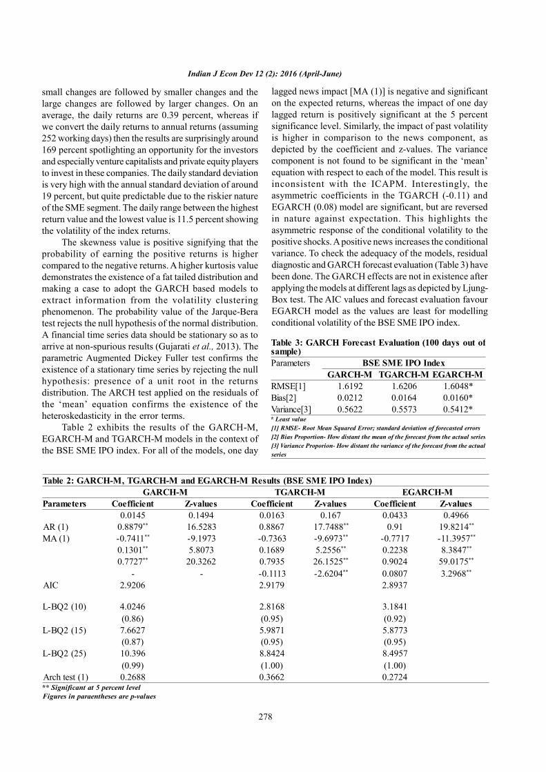
278
Indian J Econ Dev 12 (2): 2016 (April-June)
small changes are followed by smaller changes and thelarge changes are followed by larger changes. On anaverage, the daily returns are 0.39 percent, whereas ifwe convert the daily returns to annual returns (assuming252 working days) then the results are surprisingly around169 percent spotlighting an opportunity for the investorsand especially venture capitalists and private equity playersto invest in these companies. The daily standard deviationis very high with the annual standard deviation of around19 percent, but quite predictable due to the riskier natureof the SME segment. The daily range between the highestreturn value and the lowest value is 11.5 percent showingthe volatility of the index returns.
The skewness value is positive signifying that theprobability of earning the positive returns is highercompared to the negative returns. A higher kurtosis valuedemonstrates the existence of a fat tailed distribution andmaking a case to adopt the GARCH based models toextract information from the volatility clusteringphenomenon. The probability value of the Jarque-Beratest rejects the null hypothesis of the normal distribution.A financial time series data should be stationary so as toarrive at non-spurious results (Gujarati et al., 2013). Theparametric Augmented Dickey Fuller test confirms theexistence of a stationary time series by rejecting the nullhypothesis: presence of a unit root in the returnsdistribution. The ARCH test applied on the residuals ofthe ‘mean’ equation confirms the existence of theheteroskedasticity in the error terms.
Table 2 exhibits the results of the GARCH-M,EGARCH-M and TGARCH-M models in the context ofthe BSE SME IPO index. For all of the models, one day
lagged news impact [MA (1)] is negative and significanton the expected returns, whereas the impact of one daylagged return is positively significant at the 5 percentsignificance level. Similarly, the impact of past volatilityis higher in comparison to the news component, asdepicted by the coefficient and z-values. The variancecomponent is not found to be significant in the ‘mean’equation with respect to each of the model. This result isinconsistent with the ICAPM. Interestingly, theasymmetric coefficients in the TGARCH (-0.11) andEGARCH (0.08) model are significant, but are reversedin nature against expectation. This highlights theasymmetric response of the conditional volatility to thepositive shocks. A positive news increases the conditionalvariance. To check the adequacy of the models, residualdiagnostic and GARCH forecast evaluation (Table 3) havebeen done. The GARCH effects are not in existence afterapplying the models at different lags as depicted by Ljung-Box test. The AIC values and forecast evaluation favourEGARCH model as the values are least for modellingconditional volatility of the BSE SME IPO index.
Table 3: GARCH Forecast Evaluation (100 days out ofsample)Parameters BSE SME IPO Index
GARCH-M TGARCH-M EGARCH-MRMSE[1] 1.6192 1.6206 1.6048*Bias[2] 0.0212 0.0164 0.0160*Variance[3] 0.5622 0.5573 0.5412** Least value[1] RMSE- Root Mean Squared Error; standard deviation of forecasted errors[2] Bias Proportion- How distant the mean of the forecast from the actual series[3] Variance Proporion- How distant the variance of the forecast from the actualseries
Table 2: GARCH-M, TGARCH-M and EGARCH-M Results (BSE SME IPO Index)GARCH-M TGARCH-M EGARCH-M
Parameters Coefficient Z-values Coefficient Z-values Coefficient Z-values0.0145 0.1494 0.0163 0.167 0.0433 0.4966
AR (1) 0.8879** 16.5283 0.8867 17.7488** 0.91 19.8214**
MA (1) -0.7411** -9.1973 -0.7363 -9.6973** -0.7717 -11.3957**
0.1301** 5.8073 0.1689 5.2556** 0.2238 8.3847**
0.7727** 20.3262 0.7935 26.1525** 0.9024 59.0175**
- - -0.1113 -2.6204** 0.0807 3.2968**
AIC 2.9206 2.9179 2.8937
L-BQ2 (10) 4.0246 2.8168 3.1841(0.86) (0.95) (0.92)
L-BQ2 (15) 7.6627 5.9871 5.8773(0.87) (0.95) (0.95)
L-BQ2 (25) 10.396 8.8424 8.4957(0.99) (1.00) (1.00)
Arch test (1) 0.2688 0.3662 0.2724** Significant at 5 percent levelFigures in paraentheses are p-values
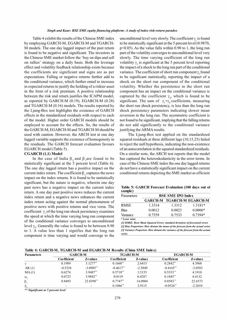
279
Table 4 exhibit the results of the Chinese SME indexby employing GARCH-M, EGARCH-M and TGARCH-M models. The one day lagged impact of the past returnis found to be negative and significant. The investors inthe Chinese SME market follow the ‘buy on dips and sellon rallies’ strategy on a daily basis. Both the leverageeffect and volatility feedback relationship exists becausethe coefficients are significant and signs are as perexpectations. Falling or negative returns further add tothe conditional variance, which further entail to increasein expected returns to justify the holding of a riskier assetin the form of a risk premium. A positive relationshipbetween the risk and return justifies the ICAPM model,as reported by GARCH-M (0.19), EGARCH-M (0.28)and TGARCH-M (0.16) models. The results reported bythe Ljung-Box test highlights the existence of GARCHeffects in the standardized residuals with respect to eachof the model. Higher order GARCH models should beemployed to account for the effects. So, the results ofthe GARCH-M, EGARCH-M and TGARCH-M should beused with caution. However, the ARCH test at one daylagged variable supports the existence of homogeneity inthe residuals. The GARCH forecast evaluation favoursEGARCH model (Table 5) .CGARCH (1,1) Model
In the case of India 2 and 3are found to bestatistically significant at the 5 percent level (Table 6).The one day lagged return has a positive impact on thecurrent index return. The coefficient 2 captures the newsimpact on the index returns. It is found to be statisticallysignificant, but the nature is negative, wherein one daypast news has a negative impact on the current indexreturn. A one day past positive news reduces the currentindex return and a negative news enhances the currentindex return acting against the normal phenomenon ofpositive news with positive returns and vice versa. Thecoefficient 1 of the long run shock persistency examinesthe speed at which the time varying long run componentof the conditional variance converges to unconditionallevel 0. Generally the value is found to be between 0.90to 1. A value less than 1 signifies that the long runcomponent is time varying and would converge to the
unconditional level very slowly. The coefficient 1 is foundto be statistically significant at the 5 percent level (0.9870,p<0.05). As the value falls within 0.90 to 1, the long runpart of the volatility converges to unconditional level veryslowly. The time varying coefficient of the long runvolatility 2 is significant at the 5 percent level reportingthe impact of a shock to the long run part of the conditionalvariance. The coefficient of short run component 3 foundto be significant statistically, reporting the impact of ashock on the short run component of the conditionalvolatility. Whether the persistence in the short runcomponent has an impact on the conditional variance iscaptured by the coefficient 4, which is found to besignificant. The sum of 3+4 coefficients, measuringthe short run shock persistency, is less than the long runshock persistency parameters indicating slower meanreversion in the long run. The asymmetric coefficient isnot found to be significant, implying that the falling returnsdo not add significantly to the conditional variancejustifying the ARMA results.
The Ljung-Box test applied on the standardizedsquared residuals at three different lags (10,15,25) failedto reject the null hypothesis, indicating the non-existenceof an autocorrelation in the squared standardized residuals.On a similar note, the ARCH test reports that the modelhas captured the heteroskedasticity in the error terms. Incase of the Chinese SME index the one day lagged returnsdo not have a statistically significant impact on the currentconditional returns depicting the SME market as efficient
Table 5: GARCH Forecast Evaluation (100 days out ofsample)Parameters BSE SME IPO Index
GARCH-M TGARCH-M EGARCH-MRMSE 1.3314 1.3312 1.3181*Bias 0.0012 0.0023 0.0006*Variance 0.7559 0.7533 0.7394** Least value[1] RMSE- Root Mean Squared Error; standard deviation of forecasted errors[2] Bias Proportion- How distant the mean of the forecast from the actual series[3] Variance Proporion- How distant the variance of the forecast from the actualseries
Singh and Kaur: BSE SME equity financing platform: A study of index risk-return paradox
Table 4: GARCH-M, TGARCH-M and EGARCH-M Results (China SME Index)Parameters GARCH-M TGARCH-M EGARCH-M
Coefficient Z-values Coefficient Z-values Coefficient Z-values 0.1989 3.1277** 0.1660** 2.6415 0.2842** 4.3968AR (1) -0.5354 -3.0985** -0.4617** -2.5849 -0.4165** -3.0583MA (1) 0.6274 3.9487** 0.5710** 3.5153 0.5333** 4.1918
0.0723 3.9842** 0.0119 0.4287 0.1845** 4.4132
0.8493 22.8398** 0.7747** 14.0904 0.8583** 22.6573 - - 0.1086** 2.9115 -0.0526** -2.2654** Significant at 5 percent level

280
Indian J Econ Dev 12 (2): 2016 (April-June)
(Table 6). The news impact on the index return is foundto be significant at the 5 percent level. The coefficient ispositive in nature, wherein a positive news adds to thecurrent index return and vice versa, contrary to the IndianSME markets. All the coefficients in the variance equationare found to be statistically significant at the 5 percentlevel except for the coefficient 2 capturing the timevarying long run component of the conditional variance.The initial effect of a shock is not found to be significanton the long run component. The sum of 3+4 coefficientsmeasuring the short run shock persistency is less thanthe long run persistence component signifying a slowerreversion to the mean level. An initial impact of a shockon the short run component only has been observed incomparison to the Indian SME market, wherein the impactof a shock has been observed on both the long run andshort run components. The asymmetric coefficient isfound to be statistically significant at the 5 percent levelindicating the existence of leverage effect in the indexreturns. A positive or negative return does not have asymmetric impact on the conditional variance. Thenegative returns increases the conditional variance incomparison to the positive returns in the Chinese SMEmarket. The Ljung-Box test and the ARCH tests confirmhomoskedasticity in the standardized residuals.Furthermore, the expected long run and short run volatilitycomponents are used to explore the relationship betweenthe index returns and the expected long run and shortrun component of volatility coupled with the unexpectedpart as well. Table 7 reports the results of the return andrisk relationship in the Indian SME segment as well asthe Chinese SME segment.
The expected long run volatility in the Indian SMEmarket has a significant negative impact on the actualindex returns, whereas the expected short run componentof the volatility has a positive impact on the index returns.Similar types of results are observed when we tried torelate the expected risk (long run and short run) with theexpected returns. Considering the SME segment as ariskier venture, the long run component of the volatilitymakes the investors to expect a reduced index return.But the short run component of the volatility increasesthe index returns, highlighting the expectations of theinvestors for a risk premium for holding the securities inthe short run. The unexpected part in the conditionalvolatility is found to be statistically significant and positivenature, making the investors to expect a risk premium inthe context of actual index returns as the expected returnsreduce for a temporary phase.
Table 7: Risk-Return parametersBSE SME IPO Index China SME Index
Parameters ActualReturns
ExpectedReturns
ActualReturns
ExpectedReturns
-0.1515** -0.0586** 0.0183** -0.0170**
(0.0002) (0.0116) (0.04) (0.00006) 0.2404** 0.1579** -0.0201 -0.0519**
(0.0000) (0.0000) (0.2482) (0.0000) 1.0472** -0.0132 1.5826** 0.0031
(0.0000) (0.2189) (0.0000) (0.50)** Significant at 5 percent level.Figures in paraentheses are p-values
Table 6: Asymmetric ARMA (1, 1) CGARCH (1, 1)resultsParameters BSE SME IPO Index China SME Index
Coefficient Z-values Coefficient Z-values
0.8971** 21.2942 -0.4584 -2.7282
-0.7462** -10.4787 0.528** 2.0891 1.4942** 4.3159 2.3728** 16.6709 0.987** 191.0444 0.8969** 20.3186 0.028** 3.2724 0.1032 0.5756 0.2185** 4.3842 -0.1573** -2.1910 0.4859** 4.3057 0.8396** 5.8152 -0.102 -1.462 0.1424** 3.3525+ 0.7044 0.6823AIC 2.9006 3.756L-BQ2 (10) 2.6946 10.907
(0.95) (0.21)L-BQ2 (15) 6.1299 15.255
(0.94) (0.29)L-BQ2 (25) 9.5406 22.174
(0.99) (0.51)Arch test (1) 0.8755 0.3045** Significant at 5 percent level
In the case of the Chinese SME segment (table 7),the expected long run component of the conditionalvolatility is significant at the 5 percent level. Therelationship between the expected returns and expectedpermanent component is negative in nature, stating thatthe long term volatility reduces the expected returns,whereas the impact of the expected long run componentis positive on the actual returns, which combats the longterm risk factors of the investors. On the other hand, therelationship between the expected short run volatility andexpected returns is negative and significant at the 5 percentlevel. The impact of the expected short run componenton the actual returns is not statistically significant depictingthat only the long term volatility has an impact on theactual returns. The unexpected part of the volatility has asignificant positive impact on the actual index returns.CONCLUDING REMARKS
The Indian investors in the SME segment witness apositive risk and return relationship in the short run,whereas a negative risk and return relation has beenobserved between the long run volatility component and

281
the index return. A reduced index return due to theexistence of long run volatility may discourage theinvestors to invest from a longer term perspective. Theinvestors should discount the information well in advanceand act accordingly in the adjustment of their portfolios.On the other hand, the case is quite interesting in theChinese SME market where the impact of a shock on thelong run component of the volatility is not statisticallysignificant, but the long run component adds to the indexreturns, due to the expectations of a risk premium. Whilethere has been a significant impact of a shock on theshort run volatility component yet that volatilitycomponent do not have a statistically significant impacton the index returns. So it’s only the long run volatilitythat shapes the Chinese SME index returns, whereas, inthe context of the Indian SME segment, both the longrun and short run volatility component contributes to thereturns but with an opposite direction. On the other hand,results reported by the GARCH-M, EGARCH-M andTGARCH-M model in the context of the BSE SME IPOindex shows insignificant, but positive relationshipbetween the risk and return, whereas a positive significantrelationship has been observed between risk and returnin case of Chinese SME segment. A positive shock has amore pronounced impact on the conditional variance incase of BSE SME IPO segment as compared to ChineseSME segment, wherein a negative shock increasesconditional volatility justifying leverage effect and volatilityfeedback hypothesis. The results reported by the risk-return dynamics, revealed a fact that a properestablishment of the Indian SME platform is going totake a longer period of time. The investors should get apart as a risk premium for investing in riskier venturesfor longer term. A lot more should be done on thetransparency, corporate governance norms, financialstatement disclosure, etc. so as to enhance the investors’confidence. This would further improve the opportunitiesavailable to the prospective companies to raise funds fromthe segment.REFERENCESAkgiray, V. 1989. Conditional heteroscedasticity in time series
of stock returns: Evidence and forecasts. Journal ofBusiness. 62 (1): 55-80.
Alom, F., Ward, B.D. and Hu, B. 2012. Modelling food pricevolatility and testing heat waves and/or meteor showersefffects: Evidence for Asia and Pacific. Asian SocialScience. 8 (12): 1-20.
Anonymous. 2012. Micro, small and medium enterprisefinance in India. International Finance Corporation (IFC).Washington, D.C., United States. Available atwww.intellegrow.com.
Anonymous. 2013. Economic Survey, 2012-13. Ministry ofFinance, Government of India, New Delhi.
Anonymous. 2013a. Recent trends in SME and
entrepreneurship finance. OECD, financing SMEs andentrepreneurs 2013: An OECD Scoreboard, OECDPublishing. Paris, France.
Anonymous. 2014. SME access to finance in the Euro area:Barriers and potential policy remedies. EuropeanCentral Bank Monthly Bulletin: 79-97.
Badhani, K.N. 2007. Intertemporal risk return relationship instock indices with alternative model specifications. TheIUP Journal of Applied Finance. 13 (7): 5-22.
Bhattacharjee, S. and Chakrabarti, D. 2013. Financialliberalization, financing constraint and Indianmanufacturing sector. Economic and Political Weekly.48 (6): 61-67.
Black, F. 1976. Studies in stock price volatility changes. InProc. of the 1976 Meetings of the American StatisticalAssociation: 171–181.
Bollerslev, T. 1986. Generalised autoregressive conditionalheteroskedasticity. Journal of Econometrics. 31: 307-327.
Bowman, E.H. 1980. A risk/return paradox for strategicmanagement. Working paper, Sloan School ofManagement.
Breen, W., Glosten, L.R. and Jagannathan, R. 1989. Economicsignificance of predictable variations in stock indexreturns. Journal of Finance. 44: 1177-1189.
Campbell, J.Y. 1987. Stock returns and the term structure.Journal of Financial Economics. 18: 373-399.
Christie, A.A. 1982. The stochastic behavior of common stockvariances: Value, leverage and interest rate effects.Journal of Financial Economics. 10: 407-432.
Dalberg. 2011. Report on support to SMEs in developingcountries through financial intermediaries. availableat http://www.eib.or (accessed 1st January, 2015)
Ding, S., Granger, C.W.J., and Engle, R.F. 1993. A long memoryproperty of stock market returns and a new model.Journal of Empirical Finance. 1 (1): 83-106.
French, K.R., Schwert G.W., and Stambaugh, R.F. 1987.Expected stock returns and volatility. Journal ofFinancial Economics. 19: 3-30.
Glosten, L., Jagannathan, R., and Runkle, D. 1993. On therelation between expected value and the volatility of thenominal excess return on stocks. Journal of Finance.48 (5): 1779-1801.
Gopal, M. and Jain, N. 2007. Impact of exchange ratefluctuations: Options for SMEs. FISME policy paper. 1:1-8.
Grover, A. and Suominen, K. 2014. Summary-State of SMEfinance in the United States. Available atwww.growadvisors.com.
Gujarati, D., Porter, D. and Gunasekar, S. 2013. Basiceconometrics. McGraw Hill Education (India), New Delhi.
Hwang, S. and Pereira, P.L.V. 2006. Small sample properties ofGARCH estimates and persistence. The EuropeanJournal of Finance. 12 (6-7): 473-494.
Kaur, P. and Singh, A. 2015. Investigating the leverage effectand volatility in the BRI C countries’equity markets after
Singh and Kaur: BSE SME equity financing platform: A study of index risk-return paradox

282
Indian J Econ Dev 12 (2): 2016 (April-June)
the U.S. financial crisis. The Journal of WealthManagement. 17 (4): 93-100.
Kharchenko, I. and Tsvetkov, P. 2013. Estimation ofvolatilities and spillover effects between developed andemerging market economies. Department of Economics,Lunds University. Sweden.
Kumar, R. and Dhankar, R.S. 2009. Asymmetric volatility andcross correlations in stock returns under risk anduncertainty. Vikalpa: The Journal for Decision Makers.34 (4): 25-36.
Lim, J. J., Mohapatra, S. and Stocker, M. 2014. Tinker, taper,QE, bye? The effect of quantitative easing on financialflows to developing countries. available at http://www.sanketmohapatra.com. Accessed on 15th May, 2015.
Linter, J. 1965. Volatility of risky assets and the selection ofrisky investments in stock portfolio and capital budget.Review of Economics and Statistics. 47: 13-37.
Majumdar, R. 2014. Indebtedness in the small and mid capsegments: New evidences from Indian manufacturingsector. Decision. 41 (1): 99-115.
Merton, R.C. 1973. An intertemporal capital asset pricingmodel. Econometrica. 41: 867-887.
Merton, R.C. 1980. On estimating the expected return on themarket: An exploratory investigation. Journal ofFinancial Economics. 8: 323-361.
Mossin, J. 1966. Equilibrium in capital asset market.
Econometrica. 35: 768-783.Naso, C. 2014. 5 Ditch IPO plans this week as markets continue
volatility. available at www.law360.com. Accessed on 15th
November, 2014.Nelson, D.B. 1991. Conditional heteroskedasticity in asset
returns: A new approach. Econometrica. 59 (2): 347-370.
Raj, B. 2012. Challenges in SME financing: Developingalternative financing source. available at www.skoch.org.Accessed on 15thFebruary, 2015.
Sharpe, W.F. 1964. Capital asset prices: A theory of marketequilibrium under conditions ofrisk. Journal ofFinance. 19 (3): 425-442.
Sharma, R. 2012. Problems and prospects of small scaleindustrial units (A case study of exporting and non-exporting units in Haryana). Asia Pacific Journal ofMarketing & Management Review. 1 (2): 191-210.
Snijder, A. 2013. The financing problems of SMES in theNetherlands. available at www.keijsercapital.nl. Accessedon 15th June, 2015.
Tripathy, N. 2008. Private equity-gaining momentum.Vilakshan XIMB Journal of Management. 5 (1): 147-156.
Whitelaw, R. F. 1994. Time variations and covariations in theexpectations and volatility of stock market returns.Journal of Finance. 49: 515-541.
283
Indian Journal of Economics and DevelopmentVolume 12 No.(2): 283-292
April-June, 2016DOI: 10.5958/2322-0430.2016.00137.2
www.soed.in
Level of Income, Expenditure Behaviour and Poverty amongFarming Community in Rural BiharGhanshyam Panday*
Agriculture Economics Research Unit, Institute of Economic Growth, New Delhi,
*Corresponding author’s email: [email protected]
Received: January 14, 2016 Accepted: May 25, 2016
ABSTRACTDuring the mature green revolution period, i.e., 1980s the trends of agricultural sector shows a favourable growth inBihar as compared to some major state even. However, increasing costs and declining farm income of the farmingcommunity in Bihar is not enough to cater to their farm and domestic expenditure, and hence a lot of people migrated fromthe state for the livelihood survive. Still Bihar is the one of the poorest state in the countryside, even a big hope foragriculture development. The present study examined the income, expenditure pattern and its distribution with povertyprevailing among the different farm size categories in rural areas of Bihar. A significant variation in the income andexpenditure level of different farm-size categories was observed. It shows the underdevelopment of the state, where morethan 60 per cent of the expenditure occurred on the non-durable items for the farmers. The small farmers were left with noamount of surplus compared to the larger farmers. It is a pity that about 64 per cent of the average farmers were below thepoverty line in the state during 2010-11. Ensuring effective distribution, allocation and implementation of variouswelfare schemes in order to brace the smaller farmers is a matter of prime concern and if left unattended will drag theeconomy of Bihar towards ambiguous development, where there is only one source of income in the absence of industriesand other sectors as well.
KeywordsIncome, expenditure, farmers, poverty, Bihar
JEL CodesD12, D24, H31, I30, R12
INTRODUCTIONAgriculture is the prime source of wealth in Bihar
and is the key to the overall development of the stateeconomy. Even at the national level, it is now widelyrecognized that high growth in agriculture is essentialfor stimulating high productivity of the non agriculturalsector to bring the desire improvement of thesociaoeconomic conditions of a large section of thepopulation (Kumar, 2011). Agriculture sector of the statenot performed as it was expected and still its lackingbehahind of the productivity of major food grains eventhis sector is backbone of the overall economy of thestate is going to the backfoot (Pandey, 2012). At the timeof independence, Bihar’s socio-political and economicsituation was not as depressing as it has gradually reachedtoday. Bihar was not only a politically stable state, but italso enjoyed the reputation of being one of the best
administration state in the 1950s; it has the legacy ofsound infrastructure in irrigation, power and industry andit registered an annual compound growth rate of 3.95percent as compared to the all-India growth rate of 3.3percent in the 1950s (Prasad, 2007). Bihar’s per capitaGDP was quite high relative to India’s in the early 1960sand, in fact, remained so well into the 1970s. It wasduring the 1980s that Bihar failed to grow fast enough tokeep up with the rest of the country. During that decade,Bihar’s rate of growth was 2.3 percent, while India’saveraged 3.2 percent. In fact, it was actually during thesecond-half of the decade, when the pre-liberalization erahad begun in India that Bihar fell dramatically behind. Itsrelative output per capita fell from 70 percent in 1985 to54 per cent by 1992. Once one takes into account thebifurcation of the state and subsequent decline in per capitaoutput, the share falls further to 43 percent. Moreover,
284
Indian J Econ Dev 12 (2): 2016 (April-June)
since 1993, which roughly coincides with the onset ofthe liberalized regime, Bihar continued to decline,bottoming out at 32 percent in 2005. Since then, it hasrecovered and in 2008 its share had risen to almost 40per cent. Thus, at least for Bihar, the story is mostly oneof divergence (Chanda, 2011).
Agriculture has played a more prominent role ofthe state, especially the bifurcation of Bihar and thecreation of Jharkhand as most of the industries andmineral resources went to later state. Bihar’s economicgrowth now depends highly on its agriculturaldevelopment. Agriculture is the main occupation of thepeople of the Bihar state. With the development ofagriculture, the socio-economic conditions of the ruralcommunity have changed significantly, and also thefinancial recuirments of the farmers surged whichincreased their dependency on outside finding. Farmingdemands regular outflow of cash to aquire variousagriculture inputs but the inflow of the same is notcontinueous due to seasonal nature of agriculture (Singhet al., 2013). However, agriculture in the state hasremained stagnant, though endowed with good soil,adequate rainfall and good ground water availability, richin nutrients such as nitrogen, potash and phosphorus.The state’s has not yet realized its full agricultural potential.This stagnation has been ascribed to several factors,including the state colonial legacy (Bharadwaj, 1993;Mearns, 1999; Banerjee and Iyer. 2002), ecologicalconditions (Ballabh and Pandey, 1999), demographicpressure and most importantly, the land tenure systemand the agrarian structure it supports (Bhaduri, 1973 andPrasad, 1974). In the plight of all these situation thepresent study an attempt to examine the levels of income,pattern of domestic as well as farm expenditure withpoverty level prevalining among the different farm sizecategories in the rural area of Bihar.METHODOLOGYSampling Design
The present study has been based on multistagestratified random sampling technique. The state of Biharhas been divided into three agro-climatic zones and zonethird further divided into two sub-zones. At the first stage,keeping in view the differences in agro-climaticconditions, one district from each zone has been selected,i.e.; Sheohar district from Zone-I, Purnia district fromZone-II, Lakhisarai district from zone-III (A) and Bhojpurdistrict from Zone-III (B). From each selected districtseach development blocks have been chosen and fromeach selected blocks one village was selected randomly.Further, from each selected village, five percent of farmhouseholds were selected randomly from each farm-sizecategories. Thus total sample consists of four districts,forty two blocks, forty two villages and 528 farm
households. Out of the total farm household surveyed,78, 257, 119, 52, and 22 were landless, marginal, small,medium, and large farmers, respectively. The details onhouseholds, cropping pattern, yield, consumption,indebtedness, assets and income from the differentsources were collected through a structure schedule forthe year 2010-11. The average operational area of thesampled farmers was 3.78 acre, of which the operationalland holding of the landless and marginal farmers was2.21 and 2.62 acre respectively. The operational holdingsof the landless farmers and marginal farmers havemarginal difference due to majority of them taking landon lease basis. Even majority of marginal farmers havetinny land plot and they were near to landless. The averagesize of operational holdings was observed more than itsllmit because majority of them taken land on crop sharingbasis and partially on cash. The operational land holdingof small farmers was 4.51 Acre, and medium and largefarmers was 6.67 acre and 12.18 acre, respectively. Theaverage family size of the sampled farmers was 7.71members per household, which shows the populationpressure on agriculture in the state. It was found thatthere were positive relationship between family size andFarm-size categories in the state of Bihar.
Table 1: Sampling characteristics of the study in Bihar,2010-11Farm Categories Sample
No.Operational
holdingsFamily
sizeLandless farmers (Notowned land but takenon lease)
78 2.21 7.3
Marginal farmers (upto2.5 Acre)
257 2.62 7.34
Small farmers (2.5 -5Acre)
119 4.51 8.02
Medium farmers (5-10Acre)
52 6.67 8.23
Large farmers (> 10Acre)
22 12.18 10.5
All Sampled Farmers 528 3.78 7.71
A simple average, percentages as well as Gini’scoefficient have used to analyses the data for the study.Gini’s coefficient which is a widely-used measure toinequality because of its certain desirable properties. It isthe ratio of the area between diagonals and the Lorenzcurve to the total area under the diagonals. It expressedas:
Gini’s coefficient = {(Xi)* (Yi+1)}- {(Xi+1)* (Yi)} Where,
Xi is cumulative percentage of householdsYi is is cumulative percentage of per capita income

285
Pandey: Level of income, expenditure behaviour and poverty among farming community in rural Bihar
Xi+1 is cumulative percentage of household log onYi+1 is cumulative percentage of per capita income log
onThe larger the value of Gini’s coefficient or closer
to the coefficient value to unity i.e. 1 the greater isinequality.RESULTSAND DISCUSSIONLevel of Household Income
The mean values of farm household income of thedifferent farm-size categories are given in Table 2. Thetable shows that an average farm household earned`62,588.29 per annum in the rural Bihar. There areconsiderable differences in the levels of income earnedby the different farm-size categories. The per householdincome of landless, marginal, small, medium and largefarm-size categories has been worked out at `32,615.37,`41,954.71, `74,701.16, `1,08,617.31 and `2,35,578.09respectively. A positive relationship between the farm-size and per household income is clearly visible for thestate. The average annual household income for the largefarm-size category is found to be around seven, five,three and two times of the income of the landless,marginal, small and medium farm-size categoriesrespectively.Other Income
The other income is the income received from othersources than farm income all the off-farmsources. It consists of the cash receivedby rendering service to a particularprofession outside the farm by one or moremembers of the farmer family during thegiven year. Such income also includespension received by any family memberand the remittance received from abroador outside the state . The study reveals thaton an average other income of farmers ofthe state was `18,255.72 which was byand large positively proportionate to the
farm size. It was `8038.46 for landless farmers,`12,416.71 for marginal farmers, `24,928.56 for smallfarmers, `26,144.23 for medium farmers and `67,955.37for large farmers (Table 2).Per Capita Income
Since the family-size varies across the sampledfarming households, so it becomes relevant to look intothe per capita income levels. The information regardingper capita income earned by the different farm-sizecategories has been presented in Table 3. An averagefarming household earns per capita income of `8,117.57annually. However, there are considerable variations inthe per capita income earning among different farm-sizecategories. Although the family-size increased with anincrease in the farm-size, yet the per capita income isalso positively associated with farm-size. It has been alsofound that there were positive relationship between farm-size and other income among the rural households exceptfor marginal farmers. However, there are considerabledifferences in the range of average per capita incomeand the average household income of the various farm-size categories. The per capita income earned by the largefarm-size category is around 5 times the per capita incomeearned by the landless farm-size category. On the otherhand, the average household income earned by the large
Table 3: Per capita income from different sources of farming householdsFarm category Sources of Income
Farm businessincome
Agriculture andallied sectors
Otherincome
Totalincome
Landless farmers 2930.17 496.14 1036.84 4463.15Marginal farmers 3586.94 863.07 1264.02 5714.03Small farmers 5651.98 1893.82 1762.51 9308.31Medium farmers 7994.39 3762.85 1439.25 13196.49Large farmers 12829.9 7129.87 2476.27 22436.01All sampledfarmers
4967.26 1713.95 1436.35 8117.56
Source: Field Survey, 2010-11.
Table 2: Level of income from different sources of farming householdsSources of income Farm category
Landless Marginal Small Medium Large All SampledFarm business income 21412.81 26336.81 45358.3 65800 134713.6 38298.67
(65.65) (62.77) (60.72) (60.58) (57.18) (61.19)Agriculture and Allied Sectors 3164.11 3201.56 4414.29 16673.07 32909.09 6033.91
(9.70) (7.63) (5.91) (15.35) (13.97) (9.64)Other income* 8038.46 12416.3 24928.56 26144.23 67955.37 18255.72
(24.65) (29.59) (33.37) (24.07) (28.85) (9.64)Total income 32615.37 41954.71 74701.16 108617.3 235578.1 62588.29
(100.00) (100.00) (100.00) (100.00) (100.00) (100.00)Source: Field Survey, 2010-11.Figures in parentheses are percent to the total.* Income includes salary, pensions, remittances, hiring out labour in agriculture, custome hiring services of machinery, etc,

286
Indian J Econ Dev 12 (2): 2016 (April-June)
farm-size category is 5.02 times the income earned bythe landless farm-size category.Domestic Expenditure
The study of domestic expenditure and itsdistribution is very important as it “ provides an idea ofthe levels of living of the farm population, consumptionpattern and degree of inequalities prevaIling in the society(Singh et al., 2013). The mean values of householdconsumption expenditure of the different farm-sizecategories are shown in Table 4. The perusal of Table 4shows that annual consumption expenditure of an averagefarming household is `81,798.53. However, there areconsiderable differences in the levels of consumptionexpenditure of the different farm-size categories. Amongnon-durables, foodgrains is an important item ofconsumption and an average farming household spendsabout 31 per cent of total consumption expenditure onthis item. The proportional share of foodgrains decreasesas the farm-size increases. The Engel`s Law ofConsumption stands proved as the portion of income spenton food items diminishes with an increase in income.Milk and milk products is the second important item ofconsumption among non-durables, and an averagefarming household spends 9.36 per cent of the totalconsumption expenditure on this item. However, fish,meat, eggs, fruits and intoxicants were the items in thefood group on which the minimum amount of expenditurewas incurred.
Among durable items, major share goes to the itemof house construction, addition of rooms & major repairsaccounting 1.59 percent for an average farminghousehold. The proportional share of house construction,addition of rooms and major repairs shows a negativerelationship with farm-size. This proportion is the highestfor the landless farm-size category, (2.25 percent)followed by the marginal, small, medium and large farm-size categories. Services account for 16.39 percent ofthe total consumption expenditure for an average farminghousehold. The proportional share of services shows apositive relationship with farm-size. Among the differentservices, the percentage share is the highest for healthcare(5.10 percent) followed by education (4.68 percent),transport (2.78 percent), communication (2.59 percent),others (0.75 percent) and entertainment (0.50 percent).The field survey revealed that in the absence ofgovernment primary health care facilities at the villagelevel, mostly farmers depended upon private health care/clinic and these institutions have taken higher chargesfor their services. Ceremonies account for 12.49 per centfor an average farming household. The proportion is thehighest (15.94 per cent) for the large farm-size categoryfollowed by the medium, marginal, small and landlessfarm-size categories. This phenomenon highlights the fact
that the ownership of means of production plays animportant role in determining the levels of living of farmers.Per Capita Consumption Expenditure
After having analysed the levels of householdconsumption expenditure and consumption pattern of thedifferent farm-size categories in the rural areas of Bihar,it becomes relevant to look into the per capitaconsumption expenditure across the different farm-sizecategories due to the differences in the family-size ofthese categories in the rural areas of Bihar. The datacollected in this regard is presented in Table 5. The tableshows that the per capita consumption expenditure of anaverage farming household is `10,609.09. However, thereare considerable variations in per capita consumptionexpenditure among the different farm-size categories inthe state. The per capita consumption expenditure is thehighest for the large farm-size category (`19,991.13)followed by the medium (`15,058.73), small(`11,579.73), marginal (`9,248.15) and landless(`6,344.94) farm-size categories. As the farm-size goesup, the per capita consumption expenditure on most ofthe items also goes on increasing. The annual per capitaconsumption expenditure of the large farm-size categoryis found to be 3.15, 2.16, 1.72 and 1.32 times of thelandless, marginal, small and medium farm-size categoriesrespectively, whereas per household consumptionexpenditure of the large farm-size category is 4.53, 3.09,2.26 and 1.69 times of the per household consumptionexpenditure of the landless, marginal, small and mediumfarm-size categories respectively.Farm Expenditure Per Hectare
Table 6 describes the break-up of expenditure oncultivation per farm households by the farm-sizecategories. In the above analysis it has been shown thatthe total income increases with farm-size categories, buthere the picture is different for the per acre gross returns;the relationship is inversely related with the farm-size.Total expenditure incurred on various inputs amount to`18,676 per acre per annum. For the all farm-size takentogether, the maximum expenditure is incurred on seeds,fertilisers and pesticides jointly. As against this, an averagegross returns from cultivation per farm household peracre works out to be `10,521. This means the net incomefrom cultivation is only `10,521 per acre. There areconsiderable variations in cost of inputs used by thefarmers. The table indicates that there is negativerelationship between the cost of inputs used and farm-size categories. The total cost of inputs per acre decreaseswith the increase in size holdings of the farmers; themedium and large farm-size categories enjoying the lowercost per acre compared to the other categories of farmhouseholds.
In Bihar the use of agricultural new technology is

287
Pandey: Level of income, expenditure behaviour and poverty among farming community in rural Bihar
Table 4: Share of consumption expenditure of farmers in rural Bihar: Category-wise(Percent)
Items of consumption Landlessfarmers
Marginalfarmers
Smallfarmers
Mediumfarmers
Largefarmers
All Sampledfarmers
Non-durablesFoodgrains 46.10 35.77 29.71 24.99 19.31 31.71
(a) Cereals 42.40 31.69 25.41 20.97 16.40 27.74(b) Pulses 3.70 4.08 4.30 4.02 2.91 3.97Condiments and spices 1.85 1.84 1.84 1.67 1.25 1.75Fruits 0.29 0.69 1.03 1.54 1.29 0.94Vegetables 4.53 4.84 5.09 4.73 3.29 4.70Milk and milk products 10.89 10.74 9.20 7.72 5.63 9.36Edible oils 0.39 0.85 1.21 1.16 0.87 0.95Sugarcane products 0.94 1.09 1.24 1.34 0.91 1.13Eggs, meat & fish 0.39 0.85 1.21 1.16 0.87 0.95Tea leaves 0.13 0.23 0.29 0.28 0.23 0.25Pickles, etc. 0.51 0.62 0.69 0.65 0.49 0.62Biscuits & sweets 0.92 1.46 1.99 2.09 1.88 1.69Intoxicants 0.55 0.88 0.76 0.73 0.95 0.81Fuel and light 5.58 5.07 4.91 4.51 3.30 4.80Clothing and bedding 1.99 2.76 3.50 3.98 3.66 3.16Footwear 0.36 0.56 0.69 0.71 0.76 0.62Washing articles 0.64 0.92 1.14 1.13 0.83 0.98Dry fruits 0.18 0.50 0.94 1.19 0.93 0.73Sub-total 77.78 70.68 66.15 60.30 46.95 66.03DurablesHouse construction, addition of rooms andmajor repairs
2.25 1.83 1.52 1.33 0.70 1.59
Radio and others 0.40 0.18 0.23 0.26 0.95 0.30Watches and clocks 0.01 0.07 0.11 0.12 0.02 0.08Fans 0.00 0.04 0.14 0.22 0.15 0.10Sewing machine 0.00 0.02 0.25 0.22 0.06 0.11Furniture 0.09 0.11 0.21 0.20 0.26 0.17Utensils 0.07 0.08 0.10 0.10 0.15 0.10Cars and jeeps 0.00 0.00 0.00 0.59 0.00 0.09Motorcycles, scooters, and mopeds 0.00 14.00 1.33 1.83 3.42 1.03Bicycles 0.29 0.16 0.27 0.16 0.26 0.21Hand pump 0.00 0.16 0.15 0.47 0.66 0.24Fridge 0.00 0.00 0.09 0.00 0.00 0.02Gas 0.11 0.00 0.14 0.13 0.26 0.09Fodder cutter 0.00 0.13 0.16 0.22 0.10 0.14Phone 0.59 0.48 0.68 0.70 1.08 0.64Others 0.11 0.15 0.15 0.13 0.50 0.18Sub-total 3.92 3.53 5.53 6.68 8.57 5.08ServicesEducation 1.54 3.31 4.96 4.16 12.78 4.68Healthcare 4.94 4.72 4.62 5.53 7.21 5.10Transport 2.12 2.32 3.12 3.27 3.53 2.78Communication 1.26 2.48 3.02 2.90 2.59 2.59Entertainment 0.16 0.36 0.61 0.76 0.63 0.50Others 0.34 0.37 0.67 1.39 1.80 0.75Sub-total 10.37 13.45 17.00 18.00 28.54 16.39CeremoniesMarriages and other social ceremonies 4.58 8.14 6.55 10.60 12.04 8.22Religious ceremonies 3.35 4.20 4.77 4.41 3.90 4.27Sub-total 7.93 12.34 11.32 15.01 15.94 12.49Total consumption expenditure(`) 46366.92 67903.78 92929.79 123944.9 209906.82 81798.53Source: Field Survey, 2010-11.

288
Indian J Econ Dev 12 (2): 2016 (April-June)
Table 5: Per capita consumption expenditure of farmers in rural Bihar: Category-wise(` per annum)
Items of consumption Landlessfarmers
Marginalfarmers
Smallfarmers
Mediumfarmers
Largefarmers
All Sampledfarmers
Non-durables Foodgrains 2925.08 3308 3440.36 3763.2 3860.6 3364.65(a)Cereals 2690.52 2930.63 2942.04 3157.12 3278.35 2943.23(b) Pulses 234.56 377.37 498.32 606.07 582.25 421.41Condiments & spices 117.1 169.63 212.73 250.98 248.26 185.4Fruits 18.68 63.89 119.47 232.24 258 99.31Vegetables 287.71 447.48 589.73 712.61 657.14 498.25Milk & milk products 691.22 993.69 1065.02 1162.15 1125.54 993.26Edible oils 122.63 171.83 222.09 283.64 271.86 194.16Sugarcane products 59.43 100.62 143.71 201.63 182.25 120.21Eggs, meat & fish 24.45 78.8 139.68 174.06 174.89 100.94Tea leaves 8.56 21.65 33.82 42.1 45.67 26.18Pickles, etc. 32.54 57.35 80.03 97.96 98.91 65.83Biscuits & sweets 58.42 134.97 230.2 314.48 376.62 179.18Intoxicants 34.84 81.59 88.21 110.07 190.47 85.77Fuel & light 353.85 469.02 568.06 679.67 660.17 509.12Clothing & bedding 126.14 255.22 405.86 599.88 731.6 335.75Footwear 22.64 51.76 80 107.47 152.38 65.87Washing articles 40.63 85.44 132.29 169.97 165.36 103.58Dry fruits 11.21 45.84 108.27 178.62 186.58 77.58Sub-total 4935.21 6536.85 7659.62 9080.8 9386.36 7005.13DurablesHouse construction, addition of rooms andmajor repairs
142.8 168.78 175.49 199.76 139.39 168.31
Radio & others 25.08 16.64 26.59 38.78 189.61 32.3Watches & clocks 0.78 6.2 12.56 17.52 3.46 7.97Fans 0 3.39 16.54 32.47 30.3 10.58Sewing machine 0 1.58 28.48 33.64 12.98 11.69Furniture 5.7 10.3 24.76 30.84 51.51 17.55Utensils 4.64 7.85 11.04 15.18 30.3 10.19Cars & jeeps 0 0 0 88.78 0 9.33Motorcycles,scooters & mopeds 0 12.71 153.92 275.7 683.98 109.8Bicycles 18.24 14.89 31.3 24.29 52.81 22.35Hand pump 0 14.73 17.8 70.09 132.03 25.86Fridge 0 0 10.47 0 0 2.45Washing machine 0 0 0 0 0 0Gas 7.01 0 16.23 19.39 51.94 9.77Fodder cutter 0 11.92 19.05 33.87 19.48 14.66Phone 37.54 43.98 78.74 105.6 216.45 67.5Others 6.84 13.56 17.48 19.85 99.56 19.08Sub-total 248.68 326.58 640.52 1005.84 1713.85 539.45ServicesEducation 97.71 296.55 574.45 625.7 2554.11 496.61Healthcare 313.15 436.67 534.76 833.17 1441.55 541.09Transport 134.82 214.46 361.78 492.64 705.62 294.98Communication 80.26 229.17 349.84 436.21 518.61 274.82Entertainment 10.35 32.98 70.89 114.48 125.54 52.53Others 21.57 33.78 77.17 208.87 359.3 79.13Sub-total 657.89 1243.64 1968.9 2711.09 5704.76 1739.18CeremoniesMarriages & other social ceremonies 290.35 752.88 757.9 1596.72 2406.92 871.87Religious ceremonies 212.8 388.18 552.77 664.25 779.22 453.45Sub-total 503.15 1141.07 1310.68 2260.98 3186.14 1325.32Total Consumption Expenditure 6344.94 9248.15 11579.73 15058.73 19991.13 10609.09Source: Field Survey, 2010-11.

289
negligible among the small landholdings and even formajority of large farmers because of expensive cost andmaintenance. The agriculture in the state is still based ontraditional technology. There is inverse relationship foundby the analysis of data between the net income fromcultivation and farmsize categories. The perusal of Table6 indicates that per acre net income by the marginal andsmall farmers is highest followed by the landless, mediumand large farmers. This also raises the frequently debatedquestion of inverse relationship between farm-size andproductivity: weather, marginal and small farmers arerelatively efficient vis-à-vis larger class farmers? Asreminder it should be borne in mind that, many studieshave supported the existence of an inverse relationshipbetween farm-size and productivity (Mazumdar, 1965,Rao, 2005, Khusro, 1964, Bardhan, 1973, Sen, 1964,Rudra, 1968, Rosenzwenig and Biswanger, 1993, Saini,1969, Krishna, 1995, and Chattopadhyay and Sengupta,1997). The present study also supports the evidence ofinverse relationship between the farm-size andproductivity in agriculture of Bihar. However, many otherstudies shows that in the developed state there were apositive relationship only due to to the adoption of newtechnology in the field of agriculture. It shows that stillfarmers of the state using traditional technology/methodfor cultivation.The results presented in Table 6 show theshare expenses of different inputs on cultivation and peracre income from agriculture and allied activities for ruralBihar. The maximum expenditure incurred is on seeds,fertilisers, pesticides jointly, followed by lease rent forland, charges for machinery, labour charges and irrigationetc., for the all sampled. The above analysis alsoemphasises that the cost to maintain and feed animalsand poultry as well as net income from it, shows positiverelationship with the farm-size categories.
Table 6: Gross and net return and input cost per acre by the different farm-size categories in rural Bihar(` per annum)
Items of consumption Landlessfarmers
Marginalfarmers
Smallfarmers
Mediumfarmers
Largefarmers
All Sampledfarmers
Gross value of out put 29588 29325 29970 28471 23858 29197Total seeds, fertilizers, pesticide, etc. 6550 9339 10701 9983 8632 9268Land rent 10360 3032 793 353 0 3220Labour charges 174 1336 2249 2467 1913 1506Charges for animal 98 137 118 123 77 123Charges for mach & implements 1327 1618 1777 1710 961 1592Transport cost 307 419 464 495 391 419Marketing comm. 43 47 178 262 194 103Irrigation charge 1316 1612 1384 1212 878 1447Others 61 510 1469 2133 4816 999Total cost per acre 20236 18047 19133 18737 17861 18676Net income per acre 9351 11278 10836 9733 5996 10521Source: Field Survey, 2010-11.
Average Propensity to ConsumeThe average propensity to consume, defined as the
proportion of income spent on consumption, has beenworked out for the different farm-size categories in ruralBihar. A detailed profile of average propensity to consumeof the different farm-size categories is presented in Table7. For an average sampled farm household, the averagepropensity to consume comes to 1.30. It is more thanone for all the farm-size categories except the large farm-size category. It is 1.42, 1.61, 1.24, 1.14 and 0.89 forthe landless, marginal, small, medium and large farm-size categories respectively.
Table 7: Average propensity to consume of farmers:Category-wise
(`)Farmcategory
Averageconsumption
Averageincome
Average propensity toconsume
Landless 46366.92 32615.37 1.42Marginal 67903.78 41954.71 1.61Small 92929.79 74701.16 1.24Medium 123944.9 108617.31 1.14Large 209906.8 235578.09 0.89All sampled 81798.53 62588.28 1.3Source: Field Survey, 2010-11.
Since the average propensity to consume is greaterthan one for the landless, marginal, small and mediumfarm-size categories, it shows that these categories offarmers in rural areas of Bihar are trying to maintain aminimum level of consumption whether they can affordit or not. In order to maintain a minimum level ofconsumption, they have to obtain loans from institutionalas well as non-institutional sources. An average householdin the sample incurs an annual deficit of `19,210.25. Thehighest deficit of `25,949.07 is incurred by the marginal
Pandey: Level of income, expenditure behaviour and poverty among farming community in rural Bihar

290
Indian J Econ Dev 12 (2): 2016 (April-June)
farm-size category. The large farm-size category has asurplus of `25,671.29.Concentration of Income and Expenditure
Analysis of the concentration of farm income andexpenditure is very important for understanding the equityissue of the rural economy in general and particul forBihar, which is know for more inequality . Therefore,the pattern of the distribution of farm income andexpenditure has been worked out and given in Table 8.The results show that the lower 10 per cent of the farmholdings accounted for only 2.15 per cent and 4.2 percent of the total farm income and expenditure in the state.The share of lower fifty per cent of the farm holdings inthe total income was only 21.89 per cent and expenditurewas 31.17 per cent. Contrary to this, the share of upper10 per cent of the farm holdings in the total farm incomeand expenditure was about 31.96 per cent and 24.24 percent over the same respectively.
Table 8: Distribution of domestic expenditure andincome among farm families in BiharCumulativepercentage ofhouseholds
Householdexpenditure
Per capitaexpenditure
Householdincome
Percapitaincome
10 4.2 4.34 2.15 1.5320 9.79 10.02 5.59 4.0930 16.2 16.5 9.99 7.4440 23.17 23.72 15.38 11.8550 31.17 31.87 21.89 17.4160 40.1 41.02 29.77 24.3770 50.23 51.2 39.75 33.0280 62.07 62.78 52.22 44.2390 76.76 76.86 68.04 59.99100 100 100 100 100Gini Coefficient 0.27 0.26 0.41 0.49Source: Field Survey, 2010-11.
Table also clearly indicates that income inequality ismore as compared to the consumtion expenditure. It isalso clearly visible that the per capita income inequality ismore as compare to the household income inequalitywhich is gini coefficient 0.49 as compared to 0.41.however, the situation is opposite in the case ofexpenditure inequality, where household inequality is moreas compared to per capita expenditure.Incidence of Poverty
The alleviation of poverty in particular, andimprovement in the standard of living of the farmers ingeneral have been the vital objectives of developmentstrategies of India. Poverty is regarded as a matter oflow absolute income. A household is classified as poor ifconsumption level is below the poverty norms. In India,the welfare profile is usually measured using consumptionexpenditure of the households because income represents
potential, but not actual consumption. Poverty is thedeprivation of food, shelter, money and clothing thatoccurs when people can’t satisfy their basic needs.Poverty can be understood simply as a lack of money ormore broadly in the term of barriers to everyday life(Wikipedia). In India, the people living below the povertyline are considered poor. They are unable to procure adefined minimum level of calories. However, the way toascertain poverty has always been matter of debate inIndia.
Table 9: Incidence of poverty among farmers in ruralBiharCategories of farmers Percentage of poor farmersLandless 91.77Marginal 78.99Small 46.22Medium 15.38Large NilAll categories taken together 63.83Source: Computed from primary data
According to Tendulkar Committee’s report onPoverty, the poverty line was `530 per capita per monthfor rural Bihar during 2009-10. This poverty line isestimated for the year 2010-11 by using general consumerprice index for agricultural labourers (CPI-AL). Theconsumer price index includes food and non-food items.The CPI-AL for the year 2009-10 was `530 whichincreased to `577 during the year 2010-11. Based on thisindex the poverty line for rural Bihar is estimated as`697.55 per capita per month, which comes to be`8370.70 per capita per annum. With the updated figuresof `8370.70 per annum, the extent of rural poverty havebeen worked out by estimating the proportion of farmfamilies living below poverty line i.e. getting less than`8370.70 per capita per annum.
The table shows that as many as around 64 percent of the farm households in rural Bihar live below thepoverty line on the basis of latest Tendulkar Committeemethod of poverty. Percentage of population below thepoverty line is 91.03, 78.99, 46.24, and 15.38 percentfor the landless, marginal, small and medium farm-sizecategories respectively. However, there is no singlehousehold from large farm-size category have been foundto live below poverty line in the state. It was expectedand general perception also found for the poverty in thestate that there is an inverse relationship betweenpopulation below the poverty line and farm-size.CONCLUSION AND POLICY IMPLICATION
The dominance of agriculture in Bihar’s economyis apparent. In terms of population dependent onagriculture as well share of agriculture in the state GDP,the numbers for Bihar are significantly higher than the

291
national average and almost all other state of the countrydue to prominence of agriculture in the state’s GDP andemployment, its performance remains a central concernof policy and planning in Bihar. But unfortunately, theincome of farming community, is not enough to cater tothe needs of farm as well as domestic expenditure. Theaverage annual net income from agriculture and alliedactivities, which is calculated after deducting theexpenditure from the gross income of agriculture andallied activities, of the farmers in the Bihar state wasworked out to be `44,332.58 and that from other activitieswas `18255.72 during the year 2010-11. The incomefrom agriculture was positively realted to the size of landholding as it increased with increase in the size of landholding. However, the share of FBI is inversely relatedwith farm-size categories. While, other income was alsopositively proportionate to the size of land holding. Theannual average net income of the farmers was `62588.29.The average domestic consumption expenditure was`81798.53. However, there is a significant variation inthe income and expenditure level of different farmcategories. The larger farmers incurred more for domesticconsumption compared to the smaller farmers. Theaverage propensity to consume is more than one for allthe farm-size categories except for large farmers. Thesmaller farmers were left with meagre amount of surpluscompared to the larger farmers. It is a pity that about 81per cent of the landless farmers, 40 per cent of marginalfarmers and 18.49 per cent of the small farmers werebelow the poverty line in Bihar with an overall 36.11 percent of the farmers living below poverty line.
To reduce the gap between level of income andconsumption, income should be increase by creating non-farm employment opportunities which is totally negligiblein the state. The government should provide basis healthcentre at the ground level to reduce the burden ofexpenditures due private health care which is exploitedcharged by private clinic owner in the absence of such afacility. Agro-based and small scale industries in the statemust be given up top priority in the absence of industryin the state to improve the level of income of the farmers.Apart from it, there is also need to educate the farmersabout subsidiary occupation and consciousness so thatthey may establish their own venture, to earn theirlivelihood as well to expenditure more on productivepurposes rather than social-economic and religiousceremonies. In the state of Bihar, landholding structureis dominated by marginal and small farmers; theimplementation of land reform which was not successfulimplemented during 1960s, in the favour of marginal andsmall farmers will be helpful in increasing their farmbusiness income and so on consumption levels at al.Reducing the percentage of families below poverty line
has been a center stage issue of the state for quite a longtimes. For reducing poverty and raising income of smallfarmers, government should supply inputs like, betterquality of seeds, fertilisers, equipments etc at subsidisedrates in order to increase their productivity andproduction. Ensuring effective distribution, allocation andimplementation of various schemes in order to brace thesmaller farmers is a matter of prime concern and if leftunattended will drag the economy of Bihar towardsambiguous development.REFERENCESBallabh, V. and Pandey, S. 1999. Transitions in rice production
systems in Eastern India: Evidence from two villages inUttar Pradesh. Economic and Political Weekly. 34 (13):A111-A116.
Banerjee, A. and Iyer, L. 2002. History, institutions andeconomic performance: The legacy of colonial landtenure systems in India. The WorldBank, Washington,D.C., United States. Culled fromwww.info.worldbank.org.
Bardhan, P.K. 1973. Size, productivity and returns to Scale:An analysis of farm-level data in Indian agriculture.Journal of Political Economy. 81 (6): 1370-1381
Bhaduri, A. 1973. A study in agricultural backwardness undersemi feudalism. Economic Journal. 83: 120-137.
Bharadwaj, K. 1993. Regional differentiation in India. In: BinoyN. Verma (ed.) Agrarian relation Institutional changeand colonial Legacy. 3, Ashish Publishing House, NewDelhi.
Chanda, A. 2011. Accounting for Bihar’s productivity toIndia’s: What can we learn from recent developments ingrowth theory?. International Growth Centre. WorkingPaper 11/0759. August, 2011.
Chattopadhyay, M. and Sengupta, A. 1997. Farm size andproductivity: A new look at the old debate. Economicand Political Weekly. 32 (52): A172-A175
Khusro, A.M. 1964. Returns to scale in Indian agriculture.Indian Journal of Agricultural Economics. 19 (3/4): 51-80.
Krishna, R. 1995. Toward a theory of optimum land reform fora dualistic agriculture. In: Vijay Krishna (ed.) RajKrishna’s selected writings. Oxford University PressNew Delhi.
Kumar, A. 2011. Agriculture performance and challenges offood security in Bihar. Agricultural Situation in India.58: 609-615
Mazumdar, D. 1965. Size of farm and productivity: A problemof Indian peasant agriculture. Economica. 32 (126): 161-173.
Mearns, R. 1999. Access to land in rural India: Policy issuesand options, World Bank Policy Research Working: 2123.
Pandey, G.K. 2012. Backbone of Bihar economy on backfoot.Mainstream. 50 (34): 28-30.
Prasad, J. 2007. Bihar-Dynamics of development. A MittalPublishers, New Delhi.
Pandey: Level of income, expenditure behaviour and poverty among farming community in rural Bihar

292
Indian J Econ Dev 12 (2): 2016 (April-June)
Prasad, P.H. 1974. Reactionary role of usurer’s capital in ruralIndia. Economic and Political Weekly. 9 (32-34): 1305-1308
Rao, C.H.H. 2005. Agricultural growth, farm size, and ruralpoverty alleviation in India. Academic Foundation, NewDelhi.
Rosenzweig, M.R. and H.P. Binswanger 1993. Wealth, weatherrisk and the composition and profitability of agriculturalinvestments. Economic Journal. 103 (416): 56-78.
Rudra, A. 1968. Farm size and yield per acre. Economic andPolitical Weekly. 3 (26/28): 1041-1044.
Saini, G.R. 1969. Farm size, productivity and returns to scale.Economic and Political Weekly. 4 (26): 323-334.
Sen, A.K. 1964. Size of holdings and productivity. TheEconomic Weekly. 6 (5/7): A119-A122
Singh, S., Sharma, V.K, Kingra, H.S., and Bhogal, S. 2013.Income level, expenditure pattern and poverty amongPunjab farmers. Journal of Agriculture Developmentand Policy. 23 (2): 26-39.

293
www.soed.in
Economic Evaluation of Badrigad Watershed, UttarakhandSubhash Chandra1* and K.P. Raverkar2
1Agricultural Economics Research Centre, DSE Campus, University of Delhi, Delhi-1100072College of Agriculture, GBPUA&T Pantnagar, Uttarakhand
Corresponding author’s email: [email protected]
Received: October 20, 2015 Accepted: March 24, 2016
Indian Journal of Economics and DevelopmentVolume 12 No. 2: 293-300
April-June, 2016DOI: 10.5958/2322-0430.2016.00138.4
ABSTRACTThe economic evaluation of Badrigad watershed in Tehri Garhwal district of Uttarakhand has been evaluated in a ‘pre’and ‘post’ framework. This study used primary data of randomly selected 150 households and secondary data fromdifferent sources. Overall, the watershed development increased productivity and intensity of cropping in all seasons.Livestock population has increased considerably. The watershed development programme increased the number oftechnology users and household income in all categories of farmers (18.8 per cent). Majority of them had expressed “lackof subsidized rate input supply”, as one of the major constraint followed by others. Frequent visits of the extension workerand expansion of agriculture infrastructure should be encouraged to help increase benefit from watershed development.
KeywordsSocio-economic, cropping pattern, cropping intensity, watershed project, Uttarakhand
JEL Codes
INTRODUCTIONThe Himalayan massif is a relatively young and geo-
morphologically unstable region. It is a major contributorof run-off and sediment in the principal rivers of SouthAsia. Constitutional wisdom holds that widespreaddeforestation and population pressure have exacerbatederosion and led to increased downstream flood hazards(Datta and Virgo, 1998). Efficient and sustainable use ofnatural resources is necessary for economic development,especially in resources poor countries. More so in theagricultural dominated economies like India where twothird of the cropped area is dependent on rainfall withoutany protective irrigation facilities. These regions have longbeen the victims of neglect on the policy front. This neglectis mainly due to the concentration of public resources inthe well-endowed regions for meeting the country’s foodrequirement through irrigation development and greenrevolution technologies (Reddy, 2000).
The watershed development programme has beenconceived basically as a strategy for productivity therebysecuring the livelihoods of people inhabiting the fragileecosystems suffering from soil erosion and moisturestress. The objectives of these programme has been
focused to ensure the availability of drinking water, fuelwood, and fodder and raise the income and employmentfor farmers and landless labourers through improvementsin agriculture production and productivity (Rao, 2000).Watershed development is the overall development of aparticular region, including the development of animalhusbandry, forest, soil and water conservation, soilfertility, pasture land, agriculture and horticulture etc. Thewatershed management programmes were initiated inIndia over 35 years ago, initially with a focus on droughtprone areas. In the past several useful studies have beenconcluded to assess the socio-economic impact ofwatershed programmes (Dhyani et al., 1993, FarringtonLobo, 1997, Marothia,1997, Samra,1997, Deshpande andThimmaiah,1999, Kerr et al., 2000, Joshi et al., 2004,and Babu et al., 2004). These evaluation studies provideduseful insights on the performance of various watershedsand examining the condition for the success acrossdifferent regions.
Badrigad micro watershed (MWS) project is spreadover the 6875 ha area. The central point of the area lies inbetween 78005’ longitude and 30034’ latitude. The activitiesfor its treatment and development were undertaken by
C81, Q16, Q18, Q25, Q56, Q57, Q58

294
Indian J Econ Dev 12 (2): 2016 (April-June)
the State Department of Agriculture under IWDP program.It is located about 200 kms from district head quarterand 130 kms from block office. MWS area gets rainalmost round the year with varying amount and intensityfrom season to season. The major share of the rainfalldoes occur during the monsoon (June to September).High intensity storms and cloud bursts during rainy seasonoften cause floods in Nala/Gad taking a toll of fertile soilwith run-off. There were total of 9922 inhabitants in theBadrigad MWS area in 1389 families. Therefore this studywas designed to evaluate the socio-economic impact ofwatershed development programme in Uttarakhand.Importance of watershed development in the region
The Uttarakhand is very rich in natural resourcesespecially forest (64.6 percent) and water, as it has morethan 12000 glaciers, dense forest mountain peaks andnetwork of 8 major rivers catchment acts as the lifelinefor the entire hydrological system of Indo-Gangetic plain(Watershed Management Directorate, 2015) . The hillyparts of the state have several typical features such asundulating topography, steep slopes, poor accessibility,heavy run-off, light textured poorly fertile soils,marginality, high risk low pay off agricultural productionsystem, and poor economic conditions of the farmersetc. At the same time, mountain system is highly energized,dynamic and extremely vulnerable to unscientific landuse changes. Therefore, conservation of natural resourcesin the mountain areas is an issue of utmost concern forsustainable development and improving livelihoodsecurities. Due to the undulating topographic features themajor part of the precipitation received through rainsrushes down to ‘Bhabhar’ and ‘Tarai’ region of the stateand other plains often creating the flood situation.
Agriculture and allied enterprises are the mainstaysof the people of Uttrakhand. About 14 per cent of thearea is under cultivation and of this only 10.7 per cent isirrigated. In hilly region, the agriculture has been atsubsistence level and thus increasing population, both ofhuman and animal, exerting excessive pressure on thenatural resources. Indiscriminate exploitation of thesevaluable resources has turned the ecological situationunfavorable and unbalanced. The productivity of thecrops particularly in hilly terrains is quite low. The available
produce from the farms is just sufficient to cater theneed of the farmers for 6-10 months. Like-wise, theanimals that are backbone of hill farming are malnourisheddue to degradation of pastures and reduction in naturalvegetation. Therefore, to arrest the declining resources,boosting the crop productivity and uplifting the socio-economic conditions of the farmers, the only way toachieve these objectives is to adopt a developmentprogramme in a watershed1 mode for sustainability ofthe ecosystem.Evolution of watershed program in Uttarakhand
The concept of watershed management in the regionwas evolved after the occurrence of dreadful flood inAugust, 1978 in Northern India. The Government of Indiaappointed a working group to formulate an action planfor flood control in Indo-Gangetic basin. The CentralWorking Group (CWG) submitted its report to theGovernment of India in 1979. As per the recommendationsof Working Group, the Government of India decided totake-up plan for treatment of the catchments of variousrivers and their tributaries. In November 1981, the forestdepartment of the erstwhile Uttar Pradesh formulated anoverall development plan for treating this region. It wasdecided to get the work done on the basis of the watershedareas through a ‘Multi-disciplinary Force’ on the basis ofmicro-watershed approach. It led to establishment ofseparate WMDat state level in 1981 to carry out the workunder the principles to check the obscure problems.Subsequently watershed management projects wereundertaken in the Himalayan region of Uttar Pradesh(presently Uttarakhand) w.e.f. 1982-83 with financialassistance of World Bank and European Union. Anapproach to watershed development in the region wasevolved through I to IV generation projects (Table1).Besides above watershed development programmesfunded by external agencies, various programs fundedby the central government were also undertaken in thestate. From the information available with WMD, it isenvisaged that in Uttarakhand various projects underIWDP, DPAP, NWDPRA and River Valley programs arein vogue since the inception of state.
In the backdrop of above discussion it becameimportant to assess the impact of such a holistic approachfor area development in the state.
Table 1: Evolution of watershed development region Uttarakhand
Projects Year Aided byFirst Generation 1982-1988 European Union: South Bhagirathi Phase-I, World Bank: Himalayan IWMPSecond Generation 1988-1992 European Union: South Bhagirathi Phase-IIThird Generation 1993-2005 European Union:Doon Valley Project, World Bank: IWDP Shivalik Hills-IIFourth Generation 2004-2011 World Bank: Uttarakhand Decentralized Watershed Development Project
(GRAMYA)Source: Data compiled from various sources, including from the WMD site, Uttarakhand

295
Chandra and Reverkar: Economic evaluation of Badrigad Watershed, Uttarakhand
METHODOLOGYThe study is based on the data collected under the
study ‘Comprehensive Assessment of WatershedProgramme in India: Case Study of Watershed Programmein Uttarakhand’. Badrigad Micro Watershed project (1999-2010), one of the watershed development projectscompleted in Uttarakhand was selected considering thebudget utilization and size of the project. Badrigadwatershed had 12 watershed committees comprised 53villages of Narendra Nagar Development Block of Tehri-Garhwal district. The study used quantitative andqualitative information collected through pre-testedschedule on various socio-economic indicators andproduction aspect in two situations viz. pre-project andpost-project from various sources and participants.Though, the impact evaluation study was based mainlyon intensive sample survey conducted during 2011-12.The secondary data were collected form PIA/DRDA,revenue records, watershed committees and other relatedagencies (Anonymous, 2012 and 2013)
In order to draw sample out of 53 villages 150farmer-respondents (about 10 percent of totalbeneficiaries) were selected at randomly. The selectedfarmer-respondents on the basis of their holdings werecategorized in three size groups viz. Small (<20 Nalis or<0.40 ha), Medium (20-50 Nalis or 0.40-1.00 ha) andLarge (50 and above Nalis or > 1.00 ha). Descriptivedata analysis method was used.RESULTSAND DISCUSSIONFamily Structure on Sample Farms
The average family size for the marginal, small andlarge farmer households has been worked out at 6.33,7.24 and 7.56 persons per family in the watershed. Thefamily size was the largest in large group of farmers.The average male percentage in the family was more thanfemales (34.71 percent). The percentage of children wasthe maximum (25.13 percent) in marginal category offarmers. It decreased in the order of 22.38 in small
category and 16.61 percent in large category.Status on literacy
Literate members were found in all the categoriesof farmers, however, with varying level of education.None of the member was post graduate level in case ofmarginal farmers (Table 3). In well doing farmer’shouseholds the members were found more educated incomparison to marginal and small ones. In Badrigad MWSarea total of 37.39 per cent population was illiteratedominating more in marginal households.
Table 2: Family size and its composition among samplehouseholdsItems Size groups
Small Medium Large TotalHousehold (No.) 61 50 39 150No. of family members (Person per family)Male 2.51 3.22 3.59 3.03
(39.64) (44.47) (47.46) (43.53)Female 2.23 2.4 2.72 2.41
(35.23) (33.15) (35.93) (34.71)Children 1.59 1.62 1.26 1.51
(25.13) (22.38) (16.61) (21.76)Total 6.33 7.24 7.56 6.95
(100.00) (100.00) (100.00) (100.00)Figures in parentheses indicate percentage Source: Field survey
Table 4: Occupation status in sample householdsOccupation Size groups
Small Medium Large TotalAgriculture 141 134 113 388
(79.21) (71.66) (72.90) (74.62)Dairy 8 14 18 40
(4.49) (7.49) (11.61) (7.69)Non-farm labour 10 8 2 20
(5.62) (4.28) (1.29) (3.85)Governmentjobs
3 9 5 17(1.69) (4.81) (3.23) (3.27)
Private Jobs 11 17 11 39(6.18) (9.09) (7.10) (7.50)
Business/Trade 5 5 6 16(2.81) (2.67) (3.87) (3.07)
Total 178 187 155 520(100.00) (100.00) (100.00) (100.00)
Figures in parentheses indicate percentage to total
Table 3: Education level of sample householdsItems Size group
Small Medium Large TotalIlliterate 157 133 100 390
(40.67) (36.74) (33.90) (37.39)Primary 92 76 58 226
(23.83) (21.00) (19.66) (21.67)Middle 65 51 44 160
(16.84) (14.09) (14.92) (15.34)High school 31 53 36 120
(8.03) (14.64) (12.20) (11.51)Intermediate 24 19 25 68
(6.23) (5.25) (8.47) (6.52)Graduate 17 23 26 66
(4.40) (6.35) (8.81) (6.33)Post graduate - 7 6 13
(1.93) (2.03) (1.25)Total 386 362 295 1043
(100.00) (100.00) (100.00) (100.00)Figures in parentheses indicate percentage to total
Status of occupation and employmentIn the rural economy, the main economic activities
providing opportunities to the work force are mainly inthe sphere of agriculture, animal husbandry and nonagricultural activities. The nature of occupation of samplehouseholds is presented in Table 4. Across the farm size,

296
Indian J Econ Dev 12 (2): 2016 (April-June)
Cropping Pattern on Sample HouseholdsSince, irrigation is a basic requirement for the spread
of high yielding varieties, a shift from traditional to themodern variety and from subsistence crop to commercialcrop is the normal outcome of enhanced irrigationfacilities.Comparable data on cropping pattern followedby the sample farmers pre and post watershed arepresented in Table 6, indicates that the food cropsdominate the cropping pattern of pre and post watershed
the maximum 74.62 per cent members were involved infarming activates, followed by the number of dairy (7.69per cent). In small families, more members were engagedin government and private jobs.Cultivated Area under Irrigated and RainfedConditions
Irrigation plays an important role in increasingagricultural production, diversifying cropping pattern andimproving economic base of the farmers. The detailsshowing irrigation resources pre and post watershed inthe watershed area are shown in Table 5.
The total cultivated area in the watershed increasedfrom 130.60 to 157.39 ha during the implementationperiod indicating conversion of waste land into cultivatedland. There was reduction in rainfed area, being 2.08 percent and increase in irrigated area being 25.5 percent.
Table 5: Cultivated area under irrigated and rainfedconditions pre and post-watershed
(ha)Period Irrigated Rainfed TotalPre-watershed 81.24 49.36 130.60Post-watershed 109.04 48.35 157.39Percentage change 25.50 2.08 17.02
Table 6: Cropping Pattern followed by the households pre and post-watershed(ha)
Season/ Name of theCrop
Size groupsSmall Percentage Medium Percentage Large Percentage Total Percentage
Pre-period: KharifCereals 14.7 31.94 26.26 30.16 32.12 30.14 73.08 30.49Millets 8.10 17.6 15.38 17.66 22.68 21.28 46.16 19.26Pulses 1.90 4.13 5.44 6.25 5.06 4.75 12.4 5.18Vegetables 0.26 0.56 0.60 0.69 0.42 0.39 1.28 0.53Others 0.22 0.48 0.64 0.74 0.20 0.19 1.06 0.44RabiCereals 15.5 33.68 28.5 32.73 34.58 32.44 78.58 32.79Pulses 4.18 9.08 7.60 8.73 8.28 7.77 20.06 8.37Oilseeds 0.44 0.96 0.86 0.99 1.24 1.16 2.54 1.06Vegetables 0.18 0.39 0 0 0.39 0.37 0.57 0.24Others 0.24 0.52 0.26 0.30 0.33 0.31 0.83 0.35SummerCereals 0 0 0.60 0.69 0 0 0.6 0.25Vegetables 0.30 0.65 0.92 1.06 1.28 1.20 2.5 1.04Gross cropped area 46.02 100 87.06 100 106.58 100 239.66 100Post-period KharifCereals 11.92 22.84 23.54 23.44 30.84 25.49 66.3 24.23Millets 7.96 15.25 12.22 12.16 15.58 12.88 35.76 13.07Pulses 4.09 7.84 9.34 9.30 11.86 9.8 25.29 9.24Vegetables 1.9 3.64 5.66 5.64 4.94 4.08 12.50 4.57Others 0.72 1.38 1.74 1.73 1.04 0.86 3.50 1.28RabiCereals 16.00 30.67 32.38 32.24 37.86 31.29 86.24 31.52Pulses 4.16 7.97 8.18 8.14 7.36 6.08 19.70 7.20Oilseeds 0.26 0.50 1.20 1.19 1.16 0.96 2.62 0.96Vegetables 0.45 0.86 0.38 0.38 0.20 0.17 1.03 0.38Others 0.62 1.19 0.56 0.56 1.82 1.50 3.00 1.10SummerCereals 0 0 0 0 0.36 0.30 0.36 0.13Vegetables 3.82 7.32 5.16 5.14 7.76 6.42 16.74 6.12Others 0.28 0.54 0.08 0.08 0.20 0.17 0.56 0.20Gross cropped area 52.18 100 100.00 100.00 100.00 100.00 273.6 100.00

297
Chandra and Reverkar: Economic evaluation of Badrigad watershed, Uttarakhand
programme. The season wise cropping pattern prior toimplementation of the programme, area under Kharif was30.49, Rabi 32.79 and summer 0.25 percent cereals. Inall the reassures, the area under cereals got reduced duringthe programme execution period. The maximum decreasewas noticed in Kharif cereals. Area under Kharif pulses,increased from 5.17 to 9.24 percent. While in Rabi pulsesslight decrease was recorded. There was tremendousincrease in area under Kharif and summer vegetables. Itincreased from 1.04 (pre-programme) to 6.12 per cent(post-programme), in the case of summer seasonvegetables and from 0.53 to 4.57 percent in the case ofKharif season vegetable. Similarly, Singh (2000) andChaudhary et al. (2015) observed that the watershedprogramme helped farmers to cover more area underirrigation. Thus a comparison of the cropping patternpre and post indicated that there was a trend towardcommercialization of agriculture.Cropping Intensity
As expected, with the increase in irrigated area underwatershed and use of modern input, the intensity ofcropping as measured by the ratio of net cropped area togross cropped area increased.The details are shown inTable 7.The cropping intensity was the maximum withmarginal farmers pre and post watershed programme. Itwas lowest with the large farmers. The average croppingwas 165.5 per cent at the launch of the watershedprogramme. This increased to 189.3 percent at thecompletion of the watershed programme. The per centincrease in cropping intensity, due to watershedprogramme did not vary much across the size group offarmers. The percentage change in the intensity ofcropping at the overall level was found to be 12.57 percent.
in case of pulses. The vegetable yield increased in all theresource however, the highest increase was observed incase of summer vegetables (74.4 percent), followed byRabi season vegetables (47.5 percent) and the lowest wasin case of Kharif. Especially in the case of vegetables thehigher increase was found in case of marginal farmersfollowed by small and then large this suggests that insmall holdings, farmers put more effects that is, bettermanagement. That main reason for higher cropproductivity observed that soil moisture and fertility statusin watershed area. Similar results were reported byPokharkar et al. (2014) and Amale et al. (2015).
Table 7: Cropping intensity pre and post-watershed(Percent)
Sizegroups
Cropping IntensityPre-watershed Post-watershed Percentage
changeSmall 202.51 230.2 12.02Medium 161.94 187.8 13.76Large 132.07 150.1 12.01Average 165.51 189.3 12.57
Yield of different Crops on Sample HouseholdsComparative picture of yield rates of selected crops
pre and post implementation of watershed amongdifferent categories of sample households are presents inTable 8.The yield of most of the crops increasedremarkable due to effects mode in the watershedprogramme. The average productivity of Kharif cerealsincreased from 15.25 to 21.11 q/ha and that of Rabi cerealsfrom 11.45 to 13.96 q/ha. Similar trend was also observed
Adoption of Improved TechnologyAgricultural technologies viz. use of HYVs, fertilizers
and pesticides were adopted by a large number of farmers
Table 8: Yield of different crops pre-and post-watershedperiod
(q)Name of the crop Size groups
Small Medium Large AveragePre-watershedKharifCereals 16.37 13.55 15.83 15.25Millets 15.27 8.67 12.29 12.08Pulses 7.98 7.13 5.34 6.82Vegetables 52.69 40.33 33.81 42.28Others 7.27 7.09 7.00 7.12RabiCereals 12.09 10.96 11.30 11.45Pulses 4.85 3.90 3.92 4.22Oilseeds 2.98 6.86 8.51 6.12Vegetables 23.33 0.00 34.87 29.10Others 5.88 3.65 10.91 6.81SummerCereals - 10.00 0.00 3.33Vegetable 21.00 27.34 45.70 31.35Post-watershedKha:rifCereals 21.29 20.08 21.96 21.11Millets 10.09 10.87 10.49 10.48Pulses 9.39 9.16 8.18 8.91Vegetables 68.00 34.66 60.04 54.23Others 9.22 10.82 11.07 10.37RabiCereals 15.77 12.55 13.56 13.96Millets 6.67 11.00 5.13 7.60Pulses 5.98 5.51 8.18 6.56Oilseed 3.12 7.58 8.72 6.47Vegetables 61.56 43.42 23.75 42.91Others 19.68 12.79 19.41 17.29SummerCereals - - 9.72 3.24Vegetables 60.56 56.87 46.59 54.67Others 16.07 6.75 2.55 8.46

298
Indian J Econ Dev 12 (2): 2016 (April-June)
due to efforts made by the watershed teams. Thewatershed programme being one of such developmentscheme aim at the propagation and adoption of improvedagricultural practices in the project area. Therefore thespread effect of the programme in the area may be seenfrom the Table 9. In all the categories of farmers, thenumber of farmers adopting improved technologies wasincreased considerably. The maximum increase of 68.9percent was recorded in case of marginal farmers followedby small farmers (53.9 percent) and the lowest increasewas in case of large farmers (32.0 per cent). At the overalllevel the percentage of adoption of improved technologieswas 53.53. As far as individual technology is concernedthe highest increase (74.74 percent) was observed inpesticides use and the lowest (38.18 percent) was withfertilizer use.
Table 9: Adoption of improved technology by the samplehouseholds pre and post-watershedItems Size groups
Small Medium Large TotalPre-watershedHYV’s 12 21 26 59Fertilizers 16 24 28 68Pesticides 4 8 12 24Total 32 53 66 151Post-watershedHYV’s 40 45 35 120Fertilizers 34 41 35 110Pesticides 29 29 27 95Total 103 115 97 325Percentage increase 68.93 53.91 31.96 53.53HYV's: High yielding varieties
Livestock position on sample householdsDevelopment of the animal resources is one of the
important activities under watershed developmentprogramme. It has got special importance in the contextof generating supplementary income in the watersheddevelopment area. The watershed programme did notshow much impact on animal wealth of the area (Table10). The total livestock population in the villages increasedfrom 1800 to 1928 pre and post-watershed programme.Only some increase in number of goat, sheep and mulewas noticed during post programme survey. The numberof buffalos increased, while the number of cowsdecreased. This was observed across the group of thefarmers. This indicated that helped in the diversificationof crop-livestock mixes and reduced risks.Change in household income on sample households
Various activities of watershed programme made theimpact on the living standard of the inhabitants. The annualhousehold income presented in Table 11. Sown mean
Table 10: Adoption of improved technology by the samplehouseholds pre and post-watershedItems Size groups
Small Medium Large TotalPre-watershedCow 86 104 214 405Buffalo 64 53 68 186Bullock 92 88 81 261Goats 204 260 389 852Sheep 16 8 52 75Mule 3 6 12 21Total 465 519 816 1800Post-watwershedCow 73 91 227 391Buffalo 84 67 76 227Bullock 95 84 77 256Goats 195 272 461 928Sheep 26 10 66 102Mule 5 5 14 24Total 478 529 921 1928
Table 11: Change in household income due to watershedprogrammeSizegroups
Cropping IntensityPre-watershed Post-watershed Percentage
changeMarginal 26725 30930 13.60Small 35983 45830 21.40Large 46912 58246 19.40Average 36540 45002 18.80
household income increased in all the categories of farmersthe mean being 18.8 percent, while in the case of 21.4percent small,19.4 percent large and 13.5 percent marginalrespectively. Theses estimates further supported thatimplementation of watershed programme in the areaenabled the households contributing more to the totalhousehold income.Constraint in implementation of watersheddevelopment programme
Watershed development programme can not beimplemented smoothly without experiencing obstacles inone form or the other. Hence, the constraints as perceivedby the farmer are to be sorted out and put forth beforethe implementing agencies for taking appropriate measuresto overcome them. Table 12 show the constraints asperceived by the participating farmers have been placedin order of the rank. Of all the household surveyed,majority of them had expressed “lack of subsidized rateinput supply”, as one of the major constraint (58.67percent) followed by,” inadequate water harvestingstructure for irrigation”,(54.66 percent),” poor extensionservices” (50.67 percent),” Inadequate funds allocated

299
Chandra and Reverkar: Economic evaluation of Badrigad watershed, Uttarakhand
for the development work (48.00 percent) as perceivedby the participating farmers. Among other constraintslike ,” Irregular organization of training”,” Insufficientinfrasture facilities”, Lack of scientific motivation aboutrecommended practices, around 32 to 41 per centhousehold expressed their views in its favour.
REFERENCESAmale, A. J., Pokharkar, V. G., Kalhapure, S.P., and Yadav, D.B.
2015. Sustainable agriculture through watersheddevelopment programme: A study of Bahirwadiwatershed project, Ahmednagar, Maharashtra. IndianJournal of Economic Development. 11 (1): 207-216.
Anonymous. 2012. Watershed Management Directorate,Government of Uttarakhand, Dehradun. Culled fromwww.wmduk.gov.in
Anonymous. 2013. Statistical Dairy of Uttarakhand.Government of Uttarakhand, Dehradun. Culled fromwww.wmduk.gov.in
Babu, G., Singh, R.K., and Singh, B. 2004. Socio-economicimpact of watershed development in Kanpur.Agricultural Economics Research Review. 17: 125-130.
Choudhary, G., Pawariya, V., and Jheeba, S. 2015. Impactevaluation of cropping pattern and production patternto watershed development project in Rajasthan. IndianJournal of Economics and Development. 11 (1): 157-165.
Datta, S.K. and Virgo,K.J. 1998. Towards sustainablewatershed development through people’s participation:Lessons from the lesser Himalaya, Uttar Pradesh.India.Mountain Research and Development. 18 (3): 213-233.
Deshpande, R. S. and Thimmaiah, G. 1999. Watersheddevelopment approach and experience of NationalWatershed Development in the country. Journal of RuralDevelopment. 18 (3): 453-469.
Dhyani, B.L., Babu, R., Ram, S., Katiyar, V.S., Arora, Y.K.,Juyal, G..P., and Vishwanathan, M.K. 1993. Economicanalysis of watershed management programme in OuterHimalaya: A case study of operational research project,Fakot. Indian Journal of Agricultural Economics. 48(2): 237-245.
Farrington, J. and C. Lobo. 1997. Scaling up participatorywatershed development in India: Lessons from the Indo-German Watershed Development Programme. NationalResource Perspective. Number 17. February 1997.Overseas Development Institute, London, U.K.
Joshi, P.K., Pangare, B., Shiferaw, B., Wani, S.P., Bouma, J.,and Scott, C. 2004.Watershed development inIndia:Synthesis of past experiences and needs for futureresearch. Indian Journal of Agricultural Econmics. 59(3): 303:320.
Kerr, J., Pangare, G.., and George, P.J. 2000. An evaluation ofdryland watershed development in India . EPTDDiscussion Paper No. 68. International Food PolicyResearch Institute, Washington.
Marothia, O.K. 1997. Agriculture technology andenvironmental quality: An institutional perspective.Indian Journal of Agricultural Economics. 52 (3): 473-487.
Pokharkar, V. G., Waykar, K.R., Kalhapure, S.P., and Amale,A.J. 2014. Economic re-evaluation of Bahirwadi
Table 12: Constraints in implementation of watersheddevelopment programme
Constraints Frequency Percentage RankInadequate funds allocated forthe development work
72 48 IV
Inadequate waterharvesting structure forirrigation
82 54.66 II
Lack of subsidized rateinput supply
88 58.67 I
Poor extension services 76 50.67 IIIIrregular organization of training 61 40.66 VInsufficient infrasturcturefacilities
58 38.67 VI
Lack of scientificmotivation aboutrecommended practices
48 32 VII
CONCLUSIONS AND POLICY IMPLICATIONSThe study has concluded that the watershed
programme has resulted in area expansion, improvementin crop productivity, intensity of cropping and increasesin livestock population. Crop diversification and therebycould provide enhanced employment and form income.Agricultural technologies viz. use of HYVs, fertilizer andpesticides were adopted by a larger number of farmers.At the overall level the percentage of adoption of improvedtechnologies was 53 percent due to efforts made by thewatersheds team. Various activities of watershedsprogramme made the impact on household incomeincreased overall around 19 percent. Under watersheddevelopment programme majority of them had expressed,lack of subsidized rate input supply, as one of the majorconstraint (58.67) percent followed by other.
Farmers were more concerned about the cropcultivation as it was their primary source of income, thusfor the development of the watershed a holistic approachneeds to be practiced including the complete package ofcrop cultivation i.e. from sowing of crop till marketing.Frequent visits of the Watershed Development Team areessential for motivating local support, formation of groupfacilitating planning, implantation and evaluation.Expansion of agriculture infrastructure should beencouraged to help increase benefit from watersheddevelopment.

300
Indian J Econ Dev 12 (2): 2016 (April-June)
watershed area development project in Ahmednagardistrict. Research Review Committee Meeting,Department of Agricultural Economics, MPKV, Rahuri-2008-09: 210-222.
Rao, C.H.H. 2000.Watershed developmentin India: Recentexperience and emerging issues. Economic and PoliticalWeekly. 35 (45): 3943-3947.
Reddy,V.R. 2000. Sustainable watershed management:
Institutional approach. Economic and Political Weekly.35 (38): 3435-3444.
Samra, J.S. 1997. Status of research on watershedmanagement. Central Soil and Water ConservationResearch and Training Institute, Dehradun.
Singh, J.P. 2000. Economic evaluation of watershed. NationalInstitute of Agricultural Extension Management,Rajendranagar, Hyderabad.

301
www.soed.in
Socio-Economics of Herbal Processing Units in HimachalPradeshSukhjinder Singh1* and Sharanjit Singh Dhillon2
1C.S.I.R.- IHBT, Palampur-176061 (H.P.)2Punjab Scholol of Economics, Guru Nanak Dev University, Amritsar- 143005 (Punjab)
*Corresponding author’s email: [email protected]
Received: February 26, 2015 Accepted: March 17, 2016
Indian Journal of Economics and DevelopmentVolume 12 No. 2: 301-306
April-June, 2016DOI: 10.5958/2322-0430.2016.00139.6
ABSTRACTThe study was designed to investigate the economics of herbal industrial units in Himachal Pradesh. Most of the herbalindustries are organized as sole proprietorship followed by partnership, private, co-operative and private. Most of theentrepreneurs of herbal industrial units in H.P. were having experience between 21 to 30 years. As an entrepreneur ofherbal industry having education in ayurvedic medicine system was high as compared to not having education inayurvedic medicine system. Profitability analysis revealed that herbal processing industry is a profitable venture. Multipleregression analysis showed that explanatory variables positively affecting the gross return of herbal industry were foundto be; expenses on packaging and qualification.
KeywordsHerbal industry, Socio economic characters, Cost, Net returns, Multiple regressions
JEL CodesO13, O14, O22, O25
INTRODUCTIONThe Ayurvedic industry in India is probably the oldest
medical care system in the world. The history of herbsin ancient India is so old that the ancient form of herbalhealing has even been mentioned in the Vedas. Even today,herbal medicines play a significant role in India. A similarpractice is also prevalent in China, South East Asia andAfrica. Survey of 123 countries conducted by WHO in2001 revealed that national recognition and regulation oftraditional medicine (TM) vary greatly amongst thesecountries. However there is increasing popularity ofTraditional Medicine in the world due to its moreaffordability and proven efficacy in number of importanthealth treatment areas. At global level, 80 percentpopulation depends on traditional medicines for theirprimary health care need (Owolabi et al., 2007). Thedemand for plant based products is increasing in bothdeveloping and developed countries as these areconsidered safe for consumption and use (Kalia, 2005).
The annual turnover of the Indian herbal industry isabout `2,300 crore with a growth rate of 15 percent(Krishnan, 1998). Indian herbal market is likely to reach
`15,000 crore by 2015 (ASSOCHAM). USA, Pakistan,Germany, Japan, UK, Spain, China, France, Vietnam andMexico were the top ten destinations for India’s herbalexports since last three years from 2007-08 to 2009-10(Anonymous, 2011) . USA is at the top with 35.7 percentof India’s total herbal exports in 2009-10 followed byPakistan (10.6 percent).
Due to different agro-climatic zones, HimachalPradesh is enriched with plant diversity. State MedicinalPlants Boards (SMPB), CSIR- IHBT, Other GovernmentResearch Bodies, Universities, NGOs, etc. are doingresearch for the purpose of promotional and commercial/economic activity leading to cultivation and value additionof medicinal plants in the state.METHODOLOGY
There are 88 Ayurvedic Pharmacies in the State,which are manufacturing herbal medicines after gettingthe license from the Department of Indian Systems ofMedicine and Homeopathy (ISMH), Himachal Pradesh. 19 herbal units of the total 70 working herbal units: 3from Solan, 10 from Kangra, 3 from Paonta Sahib and 1each from Bilaspur, Chamba and Una District were
302
Indian J Econ Dev 12 (2): 2016 (April-June)
selected purposively. In accordance with the provisionof Micro, Small and Medium Enterprises Development(MSMED) Act, 2006; four of these purposively sampleindustries fall under the category of small scale industrialcategory, whereas 15 fall under the category of microindustries.
The required primary data were collected throughpersonal interview method with the help of a wellstructured and pre-tested schedule for the year 2012-13.The relevant basic information such as number of yearsof experience in herbal processing, qualification, type ofownership was collected. The data pertaining toinvestment pattern of the different units on land, building,machinery and equipments and tools etc. was alsocollected. Cost components were calculated for thedifferent items viz., raw material, electricity & diesel,repair of building, causal and permanent labour, taxespaid etc. during the year 2012-13.
Cost components for herbal processing units havebeen divided into two categories (a) fixed cost and (b)variable cost. Fixed cost included depreciation ofmachinery and equipments, rental value of building andland, permanent labour and interest on fixed capital.Variable cost includes the cost on casual labour, rawmaterials used, chemicals, transportation charges,promotional charges, fuel, electricity, repair andmaintenance, packing material, audit and account charges,postage and stationary charges, medical and otherexpenses, taxes and interest on working capital.Functional Analysis of Herbal Industries
The following form of production function equationwas used to study the resource use efficiency andinfluence of inputs on gross returns of herbal industrialunits in the state:Y= a X1
b1 X2b2 X3
b3 …………..Xnbn + eu
The above function was converted into the linearform through logarithmic transformation of all variablesand is written as:Log Y = log a + b1log X1 + b2log X2 + b3log X3 + ------ +bn log Xn +u
Descriptions, measurement and expected signs ofvariables:Dependent Variable (Y)
Gross returns of herbal industrial unit - Thedependent variable Y which represents the actual grossreturns of herbal industrial unit by respondents, is acontinuous random variable measured in Rupees.Independent Variables (Xi)X1=Depreciation on tools (`)X2= Electricity cost (`)X3= Fuel cost (`)X4=Labour cost (`)X5= Packaging cost (`)
X6= Cost of Raw Materail inputs (`): These variablesare measured in terms of amount spent ondepreciation of fixed items, electricity, fuel, labourused, packaging and raw material inputs respectively.They are measured in rupees and expected to havenegative relationship with the net returns.
X7= Processing Experience (years): This indicated thenumber of years spent in processing business.According to Omoti (2001), the primary determinantsof a potential processor’s capabilities are experiencein business and the quality of the information providedas far as extension workers are concerned. Basedon their exposure it could be adjudged that they possesgreater ability to predict possible problems and likelysolutions that result in higher income. It is thereforeexpected that the business experience will have apositive relationship with net returns.
X8 = Education (years): This refers to the level of formaleducation received by the producers. It is measuredby the year of schooling. Educational level of theproducers is expected to have positive relationshipwith the net returns since educated producers aremore likely to be business alert and possess the abilityto seize business initiatives or advantage.
RESULTSAND DISCUSSIONSSocio-Economic Characteristics of the SampledHerbal Units
It is necessary to look into the various socio-economic characteristics of sample herbal units beforeproceeding for analyzing a particular enterprise. Varioussocio-economic characteristics of sample respondents(herbal units) which include their organization andmanagement, educational status of herbal entrepreneursand experience of the enterprises in herbal processinghas been analysed and discussed in the followingsubsections:Organization and Management
The success of an industry depends on theentrepreneurs who manage it. It implies that the type ofownership and form of organization are important in ananalysis of industrial performance of agro-processingunits.
It was found during the survey that agro-processingindustrial units in the study area are organized on fivetypes of ownership viz: as sole proprietorship; as
Table 1: Type of Ownership of herbal industriesType of ownership PercentProprietary 40.00Partnership 20.00Co-operative 10.00Private 15.00Government 15.00
303
partnership; as co-operative society; as private limitedcompany and as government concern. Distribution ofunits on the basis of the form of organization is given inTable 1. It was found that 40 percent of the surveyedherbal industrial units in the state were organized as soleproprietorship: 20.00 percent as partnership: 10.00percent as cooperative: 15.00 percent as private; andanother 15.00 percent are government concerns.
Thus most of the herbal industries are being run assole proprietorship followed by partnership, private,government and co-operative.Education of Herbal Entrepreneurs in AyurvedicMedicine System
In order to analyze the educational levels of herbal-processing entrepreneurs, they are categorized into twomain categories: having education in ayurvedic medicine,and the others not having any education in ayurvedicmedicine system as given in Table 2. Majority ofentrepreneurs (63.16 percent) in herbal industry in stateof Himachal Pradesh, were having education in ayurvedicmedicine and rest (36.84 percent) were not having anyeducation in ayurvedic medicine system.
Table 2: Education of herbal enterpreursQualification (years) PercentHaving education in ayurvedic medicinesystem
63.16
Not having any education in ayurvedicmedicine system
36.84
Table 3. Experience of enterprises in herbal processingExperience (years) Percent1 to5 5.266 to 10 26.3211 to 20 26.3221 to 30 31.58More than 30 10.53
It is clear from the Table that majority of theentrepreneurs (68.43 percent) had more than ten yearsof processing experience. Thus it is expected that theirearning will be positively affected by their experience intheir field.Cost and Revenue Structure of Sampled HerbalProcessing Units
Different cost components (variable and fixed) andrevenue structure of herbal industrial units in the state ofHimachal Pradesh are indicated in Table 4. Study foundthat of the different cost components of fixed cost,depreciation of plant & machinery as percentage of totalcost (3.17 percent) was higher for small herbal units ascompared to the micro herbal units (1.41 percent):whereas for other cost components like permanent labour,interest on fixed cost and rental value of building aspercentage of total cost (6.74, 1.31 and 0.92) were higherfor micro herbal units as compared to small herbal units(1.60, 0.77, and 0.81 percent) and hence total fixed costas percentage to total cost was more (11.19 percent) formicro herbal units as compared to small herbal units (6.54percent).
Similarly, per unit cost for these different costcomponents of fixed cost were also evaluated and it wasfound that depreciation on plant & machinery, permanentlabour, interest on fixed cost and rental value of building(`2290214, `1158250.00, `553502.00 and `588831,respectively) was higher for small units as compared tomicro herbal units (`68458.00, `326031.00, `63349.00and `44509, respectively).
Raw material cost, cost of packing material, intereston variable cost and labour wages are major variable costcomponents. Variable cost as well as percentage of totalcost for different variable cost components has beenevaluated. Study found that of the different costcomponents of variable cost,- raw material cost aspercentage of total cost was almost same for small andmicro units (33.45 percent and 33.63 percent ) and costof packing material as percentage of total cost was higher(28.89 percent) for micro herbal units as compared tothe small herbal units ( 20.04 percent): whereas for othercost components like interest on total variable costs andlabour wages were higher (10.75 and 9.50 percent,respectively) for small herbal units as compared to microherbal units (10.22 and 6.23 percent, respectively). Totalvariable cost as percentage to total cost was higher (93.46percent) for small herbal units as compared to micro herbalunits (88.81 percent).
Similarly per unit cost for these different costcomponents of variable cost were also evaluated and itwas found that raw material cost, cost of packing material,interest on variable cost and labour wages were higher(`24200000.00, `14500000.00, ` 7778238.00 and
Singh and Dhillon: Socio-economics of herbal processing units in Himachal Pradesh
Experience of Enterprises in Processing HerbsYears of experience in herbal processing also plays
an important role for the success of an enterprise.Enterprises were divided into five categories on the basisof years of experience, that is, 1 to 5 years, 6 to 10years, 11 to 20 years, 21 to 30 years, 21 to 30 years andmore than 30 years and have been depicted in Table 3.There were 5.26 percent herbal units having experienceof 1 to 5 years; 26.32 percent herbal units had experienceat 6 to 10 years; 26.32 percent herbal units had experiencebetween 11 to 20 years; 31.58 percent herbal units werehaving experience between 21 to 30 years; and 10.53percent herbal entrepreneurs were having experience ofmore than 30 years in the herbal processing.

304
Indian J Econ Dev 12 (2): 2016 (April-June)
Table 4. Costs and returns in herbal processing units of Himachal Pradesh(`)
Chemicals and preservatives Small MicroFixed Cost (F.C.)Insurance premium 90500
(0.13)1000(0.02)
Rental value of land 36625(0.05)
37361(0.77)
Building rent 588831(0.81)
44509(0.92)
Depreciation on plant, machinery and other equipments 2290214(3.17)
68458(1.41)
License fee 12950(0.02)
744(0.02)
Permanent labour charges 1158250(1.60)
326031(6.74)
Interest on fixed cost 553502(0.77)
63349(1.31)
Total fixed cost (TFC) 4730872(6.54)
541452(11.19)
Variable cost (VC)Raw material 24200000
(33.45)1627740(33.63)
Sugar 3125000(4.32)
74708(1.54)
Chemicals and preservatives 2700000(3.73)
30047(0.62)
Electricity 1340000(1.85)
39636(0.82)
Fuel 575000(0.79)
151745(3.14)
Transportation charges 2275000(3.14)
51599(1.07)
Repair and maintenance charges 125000(0.17)
16892(0.35)
Labour wages 6876000(9.50)
301736(6.23)
Promotion charges 75000(0.10)
30623 (0.63)
Packing material 14500000(20.04)
1398123(28.89)
Audit and account charges 500000(0.69)
38388(0.79)
Postage and stationary 286250(0.40)
11501(0.24)
Medical and other expenditure 255350(0.35)
10869(0.22)
Taxes 3000000(4.15)
20004(0.41)
Interest on variable cost 7778238(10.75)
494469(10.22)
Total variable cost (TVC) 67610838(93.46)
4298080(88.81)
Total cost (TFC+TVC) 72341710 4839532Gross returns (Sale) 117500000 6057297Returns over variable costs 50487488 2253686Net returns 45158290 1217765Return per rupee in percent 62.42 25.16Benefit cost ratio 1.62 1.25Gross ratio 0.62 0.8Figures in parentheses indicate percentage to total cost

305
`6876000, respectively) for small herbal units ascompared to micro herbal units (`1627740.00, `1398123,`494469.00 and `301736, respectively).
Gross returns per small herbal unit (`117500000.00)was more than that of micro herbal unit (`6057297) inthe state of Himachal Pradesh as depicted in Table 4.
Returns over variable costs of small herbal industrialunits (`50487488.00) was more than micro herbalindustries (Rs. 2253686.00) in the state. Similarly, netreturns of small herbal industries (`45158290.00) weremore than micro herbal industries (`1217765.00) in thestate of Himachal Pradesh. Return per rupee from theherbal industry was 62.42 percent and 25.26 percent forsmall and micro herbal units respectively, implying thaton every rupee invested, a profit of 62 paisa for smalland 25 paisa for micro herbal units was realized. Benefit-Cost Ratio (BCR) is high (1.62) for small herbal units ascompared to micro herbal units (1.25). Since, BCR ismore than one for both micro and small enterprisesindicating that both types of enterprise are profitable.Gross ratio was calculated as 0.62 and 0.80 for smalland micro herbal processing units respectively, whichimplies that return to the herbal industry from every rupeeinvested was 62 paisa for small and 80 paisa for microherbal units.Multiple Regression Results of Sampled HerbalIndustrial Units
The results of Multiple Regression of gross returnsof Herbal Industry in the state of Himachal Pradesh arepresented in Table 5. The F-ratio value was 29.328, andwas found to be statistically significant both at 5 percentand 1 percent level of significance, which imply that themodel is adequate for use in further analysis. Thecoefficient of determination (R2) in the case of herbalunits was 0.967, which implies that the independent
variables explain at least 96.70 percent of the variabilityin gross returns of herbal industry in the study area ofHimachal Pradesh.
The coefficient of packaging expenditure was foundto be positive and significant at five per cent level ofsignificance showing thereby that with increase inexpenditure on packaging by one per cent the resultantgross return will increases by 0.758 percent.Thecoefficient of qualification of owner was also positivelyrelated to gross returns at one per cent level ofsignificance. It shows that with increase in qualificationof owner by one percent, the resultant gross returnincreases by 14.002 percent. The regression coefficientsof other explanatory variables such as electricity, labourand experience were found to be positive but non-significant. The coefficient of depreciation cost, fuel costand raw material input cost were found to be negativebut non-significant.
Therefore, the explanatory variables positively andsignificantly affecting the gross return of herbal industryin the state of Himachal Pradesh were found to be,expenses on packaging and qualification.CONCLUSIONS
The present study was undertaken with a view toanalyze the profitability as well as socio-economiccharacteristics of herbal industry in the state of HimachalPradesh. Most of the herbal industries are organized assole proprietorship followed by partnership, private,government concern and co-operative society. Majorityof the entrepreneurs (68.43 percent) had more than tenyears of processing experience. Entrepreneurs havingeducation in ayurvedic medicine system were high (63.16percent as compared to those not having education inayurvedic medicine system (36.84 percent). Building rent,depreciation of plant & machinery, permanent labour and
Singh and Dhillon: Socio-economics of herbal processing units in Himachal Pradesh
Table 5: Determinants of gross returns of herbal industry in Himachal PradeshExplanatory variables Regression coefficients Standard errorsIntercept -17.819** 7.068Depreciation -0.0882NS 0.200Electricity cost 0.413NS 0.231Fuel cost -0.0102NS 0.054Labour cost 0.452NS 0.328Packaging cost 0.758** 0.213Raw material cost -0.224NS 0.187Experience 0.289NS 0.275Qualification 14.022*** 6.230Coefficient of Multiple Determination (R2) 0.967 0.967Adjusted (R2) 0.934 0.934F-ratio 29.328 29.328*** and ** significant at one and five percent level.NS: Non-significant

306
Indian J Econ Dev 12 (2): 2016 (April-June)
interest on fixed cost are major fixed cost components;whereas raw material cost, cost of packing material,interest on variable cost and labour wages are majorvariable cost components of small and micro herbal units.Total variable cost constitutes a major share (more than80 percent) of total cost for both small and micro herbalunits. Returns over variable costs as well as net returnswere higher for small as compared to micro herbal units.Explanatory variables positively affecting the gross returnof herbal industry were found to be; expenses onpackaging and qualification.REFERENCESAnonymous. 2011. DGCIS, Pharmexcil Research 2011. Market
Size of Herbal Medicines in Various Countries. Retrieved
from www.hosted.comm100.com.Kalia, A.N. 2005. Text book of industrial pharmacognosy.
Oscar Publication, Delhi.Krishnan, R. 1998. Indian Drug Manufactured Association
Bulletin. 13: 318- 320.Omoti, U. 2001. The future of the oil palm industry in Africa
and strategies for development: The Nigerian situation.Paper prepared for the Africa Development Bank (ADB)workshop on The Future of oil palm industry in Africaand strategies for development, Cote D’ Ivoire.
Owolabi, J., Omogbai, EKI., and Obasuyi, O. 2007. Antifungaland antibacterial activities of the ethanolic and aqueousextract of Kigelia africana (Bignoniaceae) stem bark.African Journal of Biotechnology. 6 (14): 882-85.
307
www.soed.in
Analysis of Growth, Distributional Pattern and Density ofTractors in India with Special Reference to PunjabVanusha Baregal* and D.K.Grover1Department of Economics and Sociology, Punjab Agricultural University, Ludhiana-141004
*Corresponding author’s email: [email protected]
Received: November 24, 2015 Accepted: March 08, 2016
Indian Journal of Economics and DevelopmentVolume 12 No. 2: 307-314
April-June, 2016DOI: 10.5958/2322-0430.2016.00140.2
ABSTRACTTractors form an integral part of farm mechanisation and have a crucial role to play in increasing agricultural productivity.Owing to the changing dynamics globally and nationally present study was conducted to analyse the growth, distributionalpattern and density of tractors in India and Punjab. The examination of compound growth rates revealed the rate ofgrowth of tractors was higher during Period-I (1974-75 to1994-95) as compared to Period-II (1995-96 to 2010-11) bothin the country as well as in the state. Haryana, Punjab, Uttar Pradesh and Gujarat had the highest concentration oftractors. Thetractor density i.e. number of tractors per thousand hectares of net area sown in the country was observed tobe 35.74 in 2009-10 whereas in Punjab it was112.57in 2010-11.
KeywordsTractors, growth rates, distribution, tractor density
JEL CodesB23, C22, C35, O33
INTRODUCTIONIndia’s well-orchestrated Green Revolution began
in the mid sixties. It was ushered in through the adoptionof high yielding varieties, use of balanced doses ofchemical pesticides and fertilizers, expansion of irrigationfacilities. The increased use of the above purchased inputsin agriculture necessitated to raise their use efficienciesthrough mechanization. The increase in the use of humanand bullock labour and rising wage rates and cost of up-keep of bullock further made the case of farmmechanization still stronger. Agricultural machinery,particularly tractorisation helped the farmers to go fortimely land preparation and sowing of crops and intensivecultivation.
Agriculture, being seasonal in nature requires all theoperations to be completed during specific times leadingto the shortage of human labour during the peak workload periods. The crop pattern has undergone fast changesin favour of labour intensive crops like paddy and wheat.Increase in the area under cultivation, cropping intensityand increased application of higher and split dozes offertilizers have further enhanced the labour use in stateagriculture. The seasonal index of labour use was ashigh as 196.1 in October and as low as 44.3 in March
2004-05 leading to over employment/under employmentof agriculture labour at different points of time in a year(Singh and Singh, 2006). Owing to the implementationof Mahatma Gandhi National Rural EmploymentGuarantee Scheme, wages for labour throughout Indiahave gone up leading to scarcity of farm labourers forperforming agricultural operations (EPWRF, 2003). Theshortage of labour creates problems for the farmers toperform various farm operations in peak periods. Theuse of tractors, therefore, became indispensable formaking an optimal use of other resources and timelyperformance of various farm operations.
Though it has been widely recognised thatmechanisation in general and tractorisation in particularhas played a revolutionary role in modernisation ofagriculture, still tractorisation has been a controversialissue with regard to its impact on production, productivity,human employment and more importantly regarding theeconomic rationale of investment in farm machinery. Abrief review of literature on the issue highlighted that somestudies concluded that tractorisation has displaced humanlabour and created unemployment. The share ofagricultural workers continuously declined since 1981and expected to be only 5.09 percent by 2011-12 and
308
Indian J Econ Dev 12 (2): 2016 (April-June)
that of draught animal power from 27.23 percent to 6.37per cent in 2011-12. The increase in power has beenmainly through introduction of tractors, whosecontribution has increased from 7.5 percent in 1971 to51.08 percent in 2011-12 (Kulkarni, 2011). While othershowed that tractorisation shifted cropping pattern infavour of more intensive crops and therefore, createdadditional employment. As a study conducted ontractorised and non-tractorised farms in nine States ofIndia revealed that tractor-owning farms had a highercropping intensity of 137.5 per cent as compared to 131.8percent in the case of those without a tractor and therebycreating additional employment opportunities(Anonymous, 1974).
The tractor penetration level in India has been veryslow and not remained uniform throughout the country.In1980’s Punjab, Haryana and western UP constituted themajor Tractor market with 55-57 percent share of totaltractor population in the country. Whereas in1990’s,Gujarat, MP and Rajasthan have seen good growthmainly because of good successive rains coupled withchanges in cropping patterns like adoption of moreprofitable cash crops (Oilseeds, Pulses, etc.) and betterprices. The contribution of these states improved from20-22 percent in early 1990’s to 30-32 percent by theclose of the decade (2000). The share of eastern states,namely Bihar, Orissa, West Bengal and Assam had beenconsistently low at 35 percent due to various socio-economic, agro-climatic and other reasons. The creditavailability to the farmers in this area has been anothermajor reason for the slow growth in the eastern states.Maharashtra, Tamil Nadu, Karnataka and Andhra Pradeshhave shown consistent growth since mid 1980’s. Theirshare in the Indian Tractor industry, which was about14-15 percent in 1990, had increased to around 25 percent in 1997 when the farmers suffered on account ofuneven monsoons, poor cotton crops, etc. This region isexpected to contribute more than 30 per cent to the tractorindustry. This expectation is based on the fact that thefarmers in this southern region have been adopting highvalue case crops and latest crop production/ managementpractices (Jain, 2006).
Although the controversy of tractorisation, its formand extent, stands unresolved, yet there has beenconsistent increase in the demand for tractors in thecountry as well as in Punjab. The number of tractorsincreased from 0.1 million in 1971 to 2.7 million in 2004and increased to 5.8 million in 2011-12 in the country.Whereas, the numbers of tractors in Punjab were 0.047million in 1974-75 to 0.33 million in 1993-94 whichfurther increased to 0.52 million in 2011-12 (GOP 2012).In this context of new challenges and changing order inthe tractor industry, an extensive research is needed to
understand the growth pattern,distributional pattern oftractors in the country and in the state.DATAAND METHODOLOGY
The study was undertaken on a macro frameworkbased on secondary data. To meet the objectives of thisstudy, data on different variables such as number oftractors, net area sown, cultivated area, total croppedarea, irrigated area and area under high yielding varietieswere obtained from various issues of Statistical Abstractof India and Statistical Abstract of Punjab.Trend Analysis
Time series data on number of tractors in leadingagricultural states of India and Punjab for the period of1974-75 to 2010-11 were collected and the growth trendswere worked out. To study the comparative pattern ofgrowth of tractors in leading agricultural states of Indiaand in various districts of Punjab over time, the wholeperiod under the study was divided into two periods.Period-I is characterised by high rate of growth inagriculture mainly due to technological revolution thatoccurred during mid sixties and spread during this periodand where as Period-II is characterised by moderate rateof growth in agriculture .The classification is as follows:Period-I (1974-75 to 1994-95) ;Period-II (1995-96 to 2010-11) andOverall Period (1974-75 to 2010-11).
The growth of tractors in India and Punjab wasstudied through compound growth rates
(CGR), which was computed by fitting theexponential trend equation:
Y = ABt
Where,Y = number of tractorsA = constantB = regression coefficientt = time period
Compound growth rate in per cent (r) was thusestimated as under:r = (B-1)×100
The significance of growth rate was tested byapplying Students- t-statistics.Tractor Density
To see the inter-state and inter-district variations inthe tractor concentration, the percentage share of differentstates and districts in the total tractor population of thecountry and of the state was worked out. But as the sizeof different states and districts is not uniform with regardto cultivatable area, the tractor population per thousandhectares of total cropped area, net area sown, grossirrigated area, net irrigated area and area under high yieldingvariety was also worked out for three points of time.Tractor density was calculated as follows:

309
1000areasownNet
tractorsofNumberdensityTractor
RESULTSAND DISCUSSIONThe results have been discussed under the following2 heads:(i) Growth, distributional pattern and density of tractors
in India(ii) Growth and distributional patternand density of
tractors in Punjab.Growth, Distributional Pattern And Density OfTractors In IndiaGrowth of tractors
The compound growth rates of tractors in leadingagricultural states of India have been presented in Table1. The growth rates were worked out for three timeperiods, 1974-75 to 1994-95 (Period-I), 1995-96 to 2010-11 (Period-II) and 1974-75 to 2010-11 (overall).
A glance on the Table 1 revealed that the tractors inthe country increased at a rate of 12.55 per cent perannum during the Period-I but the rate of growth declinedto 6.24 per cent during the Period-II. The overall annual
rate of growth was observed to be 9.72 per cent.The state-wise analysis showed that during Period-
I (1974-75 to 1994-95), the maximum growth rate of19.52 per cent was recorded for Madhya Pradeshfollowed by Haryana (17.08 percent), Rajasthan (14.37percent) and Uttar Pradesh (13.49 percent). Among otherstates Gujarat, Maharashtra, Andhra Pradesh, Karnataka,Punjab, Kerala and Tamil Nadu had the growth rates12.66, 12.14, 11.06, 10.90, 10.85, 5.06 and 3.55 percent respectively. The growth rates in the states ofMadhya Pradesh, Haryana, Rajasthan, Gujarat and UttarPradesh were observed to be higher than the average forIndia as a whole (12.55 percent).
During the Period-II (1994-95 to 2010-11),Karnataka attained the maximum growth rate of 11.1 percent followed by Maharashtra (8.13 percent), MadhyaPradesh (7.61 percent), Andhra Pradesh and Rajasthan(6.89 percent), Uttar Pradesh (6.57 percent), Tamil Nadu(6.45 percent), Haryana (6.30 percent) and Punjab (1.90percent). Kerala showed a negative rate of growth of -0.37 per cent. The rate of growth during the period 1995-96 to 2010-11, compared to earlier period of 1974-75to1994-95 was lower in almost all the states with anexception of Karnataka and Tamil Nadu where it increasedfrom 10.47 and 2.93 per cent in Period-I to 11.13 and9.35 in Period-II (1995-96 to 2010-11) respectively.Further it was found that in the states namely Gujarat,Haryana, Maharashtra, Rajasthan, Uttar Pradesh, AndhraPradesh, Karnataka, Madhya Pradesh and Tamil Nadu,the growth rates were higher than that of India as whole(6.24 percent) during the Period-II.
When the overall picture of two periods wasanalysed, it indicated that Madhya Pradesh recorded thehighest rate of growth (13.63 percent), followed byRajasthan (12.02 percent), Haryana (11.62 percent), TamilNadu (10.35 percent), Maharashtra (10.30 percent) andGujarat (10.09 percent). The rate of growth was thelowest in Kerala (3.65 percent).
Few points clearly emerge from the precedingdiscussion. Firstly, the growth of tractors, in general,was higher during the period I (1974-75 to 1994-95) ascompared to Period-II (1995-96 to 2010-11). Thisimpressive rise in the rate of growth of tractors duringthe Period-I could be credited to the Green revolutionwhich started in mid sixties but spread during this period.Thus it was the impact of Green revolution and newtechnology that contributed significantly and positivelytowards the demand for tractors during these years (1974-75 to 1994-95). Secondly, in Period-II (1994-95 to 2010-11) it can be seen that growth has been relatively high instates where tractor penetration was low initially viz.states like Tamil Nadu and Karnataka. The more heavily
Vanusha and Grover: Analysis of growth, distributional pattern and density of tractors
Table 1: Compound growth rates of tractors in differentstates of India
(Percent)States Period I Period II OverallGujarat 12.66***
(0.73)6.74***
(0.23)10.09***
(0.33)Haryana 17.08***
(0.78)6.30***
(0.43)11.62***
(0.53)Maharashtra 12.14***
(0.60)8.13***
(0.37)10.30***
(0.26)Punjab 10.85***
(0.65)1.90***
(0.17)6.26***
(0.44)Rajasthan 14.37***
(0.92)6.89***
(0.22)12.02***
(0.41)Uttar Pradesh 13.49***
(1.0.3)6.57**
(3.29)9.36***
(0.76)Andhra Pradesh 11.06***
(0.49)6.89***
(0.22)9.51***(0.55)
Karnataka 10.90***
(0.45)11.13***
(2.87)9.70***
(0.26)Kerala 5.06***
(1.45)-0.37NS
(1.82)3.65***
(0.60)Madhya Pradesh 19.52***
(1.36)7.61***
(1.37)13.63***
(0.71)Tamil Nadu 3.55***
(0.89)6.45**
(2.34)10.35***
(0.82)Other States 9.30***
(2.26)9.35***
(1.91)10.70***
(0.81)India 12.55***
(0.42)6.24***
(0.14)9.72***
(0.29)Source: Statistical Abstract of India and Statistical Abstract of Punjab*** and ** significance at 1 and 5 percent levelNS: Non-significantFigures in parentheses are standard errors

310
Indian J Econ Dev 12 (2): 2016 (April-June)
mechanised regions particularly Punjab, Haryana, andUttar Pradesh, overtime the pace of tractorisation in thesestates had slowed down significantly reason being thatthe number of tractors have almost reached a saturationlevel from both economic as well as operational point ofview. A study conducted by Bhattathiri (2013) indicatedthat Kerala has exhibited decreased and negative growthrate overtime, mainly citing the reason of declining trendin the paddy cultivation due to escalating cost of riceproduction, hike in diesel prices etc.Distribution of tractors
It is evident that, the pattern of tractorisationwas not uniform in all the states, the relative share ofeach state in the total number of tractors of the countryhas been worked out and demonstrated in Table 2.
The number of tractors which was only 1.64 lakhduring 1974-75 increased to 53.1 lakh in 2011-12 (Table1.2). The interstate analysis for distributional pattern oftractors revealed that six states namely, Punjab, UttarPradesh, Gujarat, Rajasthan, Maharashtra and Karnatakaaccounted for about 77 per cent of the total tractorpopulation in the country during 1974-75. During 1993-94, about 79 per cent was concentrated in six states
namely, Uttar Pradesh, Punjab, Haryana, Rajasthan andGujarat and Madhya Pradesh.
In 2011-12, Uttar Pradesh, Rajasthan, MadhyaPradesh, Haryana and Punjab occupied first five positionsin terms of percentage share in the total tractor population.These states taken together accounted for about 57percent of tractor population in the country.
The most impressive fact which came out of aboveanalysis was that 40-50 per cent of total tractors in Indiawere concentrated only in two states – Punjab and UttarPradesh during 1974-75 and 1993-94 mainly because ofthe higher level of agricultural development and size ofcultivated area in these states respectively. During 2011-12, Rajasthan and Uttar Pradesh occupied more than 30per cent of the total tractors concentrated in the country.This is mainly because of higher MSP‘s, limitedavailability of labour forcing higher mechanisation ,greater availability of finance for the purchase of tractor,and increasing non- agricultural use of tractors and sizeof cultivated area in these states respectively.Tractor Density in India
The higher percentage share of any state in totaltractor population or the more tractors in terms of absolutenumber does not signify in any way the higher level oftractorisation in that particular state. The size of stateswith regard to cultivable land in India varies too much. Itis, therefore, the tractor density, that is, tractor populationper thousand hectares of total cropped area, or grossirrigated area or net area sown or net irrigated area whichpresents the comparative picture of intensity oftractorisation in different states of the country.
Tractor population per thousand hectares of totalcropped area, net area sown, net irrigated area or grossirrigated area has been worked out to have a comparativepicture of intensity of tractors in various states of India.The higher the gap between the number of tractorsavailable per thousand hectares of gross cropped area orgross irrigated area or net area sown and net irrigatedarea implied the lower level of irrigation facilities availablein a particular state.
The perusal of Table 3 showed that the number oftractors availability per thousand hectares of net area sownin India was only 1.19 in 1974-75 which moved up to11.76 in 1993-94 and 35.74 in the year 2009-10. Theinter-state analysis of tractor concentration brought outthat in the states like Madhya Pradesh, Maharashtra,Andhra Pradesh, Karnataka, Tamil Nadu and Rajasthan,the tractor availability per thousand hectares of net areasown was even less than one.
Tractor density was found to be the highest inPunjab, being 11.64 thousand hectares of net area sownfollowed by Gujarat with 2.02 tractors and Haryana with1.87 tractors per thousand hectares of net area sown.
Table2: Distribution of tractors in different states ofIndia at different points of time
(Number)States 1974-75 1993-94 2011-12Gujarat 16054
(9.79)120951(7.23)
495136 (8.53)
Haryana 6598(4.02)
192815(11.53)
516658(8.9)
Maharashtra 9260(5.65)
83088(4.96)
419291(7.22)
Punjab 47611(29.06)
338494(20.24)
518915(8.92)
Rajasthan 13444(8.20)
185576(11.09)
699881(12.05)
Uttar Pradesh 30702(18.7)
360415(21.55)
1064284(18.32)
Andhra Pradesh 6929(4.22)
50780(3.03)
342416(5.9)
Karnataka 8370(5.10)
56189(3.36)
363993(6.27)
Kerala 2466(1.50)
11675(0.69)
11602(0.2)
Madhya Pradesh 8022(4.89)
126288(7.55)
517743(8.91)
Tamil Nadu 4799(2.92)
15604(0.93)
186670(3.22)
Other States 9576(5.84)
130188(7.78)
689147(11.86)
India 163831(100.00)
1672063(100.00)
5811131(100.00)
Source: Statistical Abstract of India and Statistical Abstract of PunjabFigures in the parentheses are percentage to the total tractors in thecountry

311
The tractor population per thousand hectares of net areasown was found to be lowest in Madhya Pradesh (0.43).In the period (1993-94) too, Punjab maintained the highestposition with regard to density of tractors. It was 80.32per thousand hectares of net area sown. Haryana with54.88 tractors and Uttar Pradesh with 20.89 tractors werenext to Punjab. The other states such as Madhya Pradesh,Kerala, Maharashtra, Andhra Pradesh, Tamil Nadu,Karnataka, had less than 7 tractors per thousand hectaresof net area sown. During 2009-10, Haryana was foundto be the highest with 138.2 tractors per thousandhectares of net area sown, Punjab and Uttar Pradesh werenext to Haryana with 119.6 and 57.5 tractors, respectively.
The above description indicated that althoughincrease in tractor population (absolute number) wasobserved more or less in all the states yet number oftractors per thousand hectares of net area sown was stillvery low in some states. It was observed that the tractorpopulation per thousand hectares of net area sown indifferent states was quite skewed and varied between5.12 and 138.2 tractors per thousand hectares of net areasown in Kerala and Haryana respectively. Furthermore,it indicated that Haryana, Punjab, Uttar Pradesh andGujarat had the highest concentration of tractors whileKerala, Maharashtra, Andhra Pradesh and MadhyaPradesh were the states with lower tractor density in thecountry. The density of tractors in Haryana was thehighest at 138.2 tractors per thousand hectares of netarea sown, thereby establishing the fact that the Haryanaagriculture is highly mechanised.Growth, Distributional Pattern and Density ofTractors in PunjabGrowth of tractors
The compound growth rates of tractors in differentdistricts of Punjab have been worked out pertaining to
the periods 1974-75 to 1996-97 (Period-I), 1996-97 to2011-12 (Period-II) and 1974-75 to 2011-12 (overall),and the same have been depicted in Table 4. It wasobvious from the table that the annual compound growthrate of tractors in Punjab was 9.92 per cent during Period-I and it declined to 1.32 per cent in Period-II. The overallrate of growth over the span 1974-75 to 2011-12 wasobserved to be 5.71 percent per annum. The district-wise position revealed that all the districts recorded asignificant rate of growth in tractors throughout the periodunder review. Furthermore, it was observed that duringPeriod-I (1974-75 to 1996-97). The highest rate ofgrowth was attained by Sangrur district (16.50 percent)followed by Faridkot (14.08 percent), Rupnagar (12.23percent) and Amritsar (11.67 percent). The lowest rateof growth was recorded by Jalandhar (7.41 percent). Inthe districts Sangrur, Faridkot, Rupnagar, Amritsar andGurdaspur the growth rates was higher than the state’soverall average (9.92 percent)
In the Period-II (1997-98 to 2011-12) Hoshiarpurdistrict witnessed highest growth rate of 3.09 percentfollowed by Patiala (2.61 percent), Rupnagar (2.17percent), and Jalandhar (2.12 percent) while Faridkotshowed the lowest growth rate of 0.57 per cent perannum. The districts which showed growth rates higherthan that of state average (1.32 percent) were Hoshiarpur,Patiala, Rupnagar, Jalandhar and Kapurthala.
The overall growth rate (1974-75 to 2011-12)was maximum in the district of Sangrur (8.71 per cent)followed by Faridkot (7.7 percent), Rupnagar (7.19percent) and Amritsar (6.11 percent). The minimum rateof growth was observed for Bathinda (4.70 percent).Among other districts, Firozpur, Hoshiarpur, Gurdaspur,Patiala and Kapurthala showed growth rates of 5.72, 5.67,5.66, 5.60 and 5.22 per annum, respectively.
Table 3: Number of tractors per thousand hectares of Net area sown (NAS), Total cropped area (TCA), Net irrigatedarea (NIA), Gross irrigated area (GIA) in India and major statesStates 1974-75 1993-94 2009-10
NAS TCA NIA GIA NAS TCA NIA GIA NAS TCA NIA GIAGujarat 2.02 1.88 11.71 10.79 12.87 11.33 47.61 39.18 39.8 36.8 94.67 83.21Haryana 1.87 1.36 3.71 2.54 54.88 33.15 72.4 42.7 138.2 77.2 159.93 88.51Maharashtra 0.51 0.47 5.74 4.79 4.61 3.88 31 25.47 19.06 15.69 101.93 76.21Punjab 11.64 8.06 14.96 9.98 80.32 44.4 86.19 46.76 119.6 63.18 122.15 64.49Rajasthan 0.96 0.86 5.08 4.28 11.43 9.63 40.36 33.16 35.67 27.84 103.51 82.84Uttar Pradesh 1.79 1.35 3.94 3.34 20.89 14.1 31.16 22.02 57.5 38.52 70.88 50.48Andhra Pradesh 0.6 0.52 2.07 1.57 4.9 4 24.14 10.11 26.17 20.82 62.05 45.36Karnataka 0.81 0.76 6.61 5.62 5.2 4.51 36.03 18.91 30.64 24.76 94.05 77.84Kerala 1.12 0.81 5.3 3.78 5.21 3.83 23.62 28.26 5.12 3.99 27.62 23.43Madhya Pradesh 0.43 0.39 4.91 4.72 6.39 5.08 5.57 22.84 30.62 21.41 66.51 64.01Tamil Nadu 0.86 0.72 1.97 1.58 2.64 2.64 14.8 4.4 30.75 26.99 52.52 46.45India 1.19 1 4.86 3.92 11.76 8.96 32.4 24.36 35.74 26.04 44.91 57.91Source: Statistical Abstract of India and Statistical Abstract of Punjab
Vanusha and Grover: Analysis of growth, distributional pattern and density of tractors

312
Indian J Econ Dev 12 (2): 2016 (April-June)
Thus, one of the striking observations which cameout of above discussion was that all those districts wherethere was less number of tractors in the base period,exhibited higher rate of growth. Another point thatemerged from the above analysis was that growth ratesof tractors showed a decline in all the districts in Period-II as compared to Period-I. The higher growth ratesduring this period (Period-I) may be attributed to the‘technological revolution’ which initiated in mid sixtiesand the higher rate of growth of tractors in this period(during seventies and mid eighties) was in quick responseto the increased power requirements which wereconsequence of intensive cultivation and incredibleincrease in the cropping intensity. But in Period-II thepace of tractorisation in these state had slowed downsignificantly reason being that the number of tractors havealmost reached a saturation level from both economic aswell as operational point of view.Distribution of tractors
The district-wise position of tractor population alongwith the percentage share of each district in total tractorpopulation in the state has been presented in Table 5. Thenumber of tractors which was only 55,327 recorded a
phenomenal rise (during the period 1975 to 2012) to518915 tractors. The inter-district analysis ofdistributional pattern brought out that the districts namelyBathinda, Ludhiana, Patiala, Jalandhar, and Firozpuroccupied first five positions and these districts collectivelyconstituted approximately about 70 per cent of the tractorpopulation in the state during the period 1975-76.
During 1994-95, Firozpur, Bathinda, Faridkot,Sangrur and Ludhiana taken together accounted for about60 per cent, whereas all the remaining districts sharedonly about 40 per cent of the total tractor population inthe state. In 2011-12, 65 percent of the total tractorpopulation of the state was concentrated in the districtsof Bathinda, Firozpur, Faridkot, Sangrur, Patiala andLudhiana.
The foregoing analysis indicated that tractors in thestate were concentrated in the districts of Bathinda,Firozpur, Ludhiana, Patiala, Jalandhar, Sangrur, andFaridkot whereas Rupnagar, Gurdaspur, Hoshiarpurdistricts being sub mountainous regions had relatively lowpercentage share in total tractor population of the state.
Table5: Distribution of tractors in different districts ofPunjab at different points of time
(Number)District 1975-76 1994-95 2011-12Gurdaspur 1960
(3.54)12614(3.55)
14812(2.85)
Amritsar 3267(5.90)
32288(9.10)
39954(7.69)
Kapurthala 2709(4.90)
11979(6.94)
17224(3.32)
Jalandhar 6183(11.18)
24632(6.94)
36525(7.03)
Hoshiarpur 3361(6.07)
12858(3.62)
24403(4.70)
Rupnagar 1043(1.89)
9285(2.61)
13247(2.55)
Ludhiana 9191(16.61)
37722(10.63)
50364(9.70)
Firozpur 4021(7.27)
49278(13.89)
58832(11.3)
Faridkot 3448(6.23)
41973(11.83)
55508(10.96)
Bathinda 11752(21.24)
48448(13.66)
59437(11.45)
Sangrur 1846(3.34)
41794(11.78)
54813(10.56)
Patiala 6546(11.83)
31789(8.96)
52503(10.11)
Punjab 55327(100.00)
354660(100.00)
518915(100.00)
Source: Statistical Abstract of Punjab
Table 4: Compound growth rates of tractors in differentdistricts of Punjab
(Percent)District Period-I Period -II OverallGurdaspur 10.73***
(0.74)0.79***
(0.06)5.66***
(0.53)Amritsar 11.67***
(0.87)1.11***
(0.09)6.11***
(0.58)Kapurthala 8.45***
(0.50)1.55***
(0.13)5.22***
(0.73)Jalandhar 7.41***
(0.34)2.12***
(0.04)4.75***
(0.27)Hoshiarpur 7.45***
(0.19)3.09***
(0.10)5.67***
(0.19)Rupnagar 12.23***
(0.44)2.17***
(0.08)7.19***
(0.49)Ludhiana 7.54***
(0.38)1.20***
(0.07)4.76***
(0.30)Firozpur 11.29***
(1.29)0.61***
(0.02)5.72***
(0.67)Faridkot 14.08***
(1.46)0.57***
(0.04)7.72***
(0.77)Bathinda 7.57***
(0.17)0.84***
(0.03)4.70***
(0.29)Sangrur 16.50***
(1.22)1.23***
(0.08)8.71***
(0.82)Patiala 8.60***
(0.58)2.61***
(0.18)5.60***
(0.34)Punjab 9.92***
(0.59)1.32***
(0.04)5.71***
(0.44)Source: Statistical Abstract of Punjab*** significant at one percent levelNS: Non-significantFigures in parentheses are standard errors
Density of tractorsAs the geographical size of the districts varies from
one to another, the density of tractors was worked out to

313
Table 6: Number of tractors per thousand hectares of Net area sown (NAS), Total cropped area (TCA), Net irrigatedarea (NIA), Gross irrigated area (GIA), Area under high yielding variety (HYV) in Punjab and major districtsDistricts 1975-76 1993-94 2010-11
NAS TCA NIA GIA HYV NAS TCA NIA GIA HYV NAS TCA NIA GIA HYVGurdaspur 7.6 4.76 11.63 7.32 10.32 43.87 25.5 61.98 31.54 32.99 51.47 29.27 59.36 33.13 33.38Amritsar 8.00 5.19 8.55 5.42 9.25 69.81 37.42 69.84 37.46 50.66 182.13 93.21 182.13 93.12 105.11Kapurthala 20.37 15.84 25.06 18.45 27.64 85.5 44.07 85.24 44.07 50.76 125.23 62.15 125.23 62.05 73.6Jalandhar 21.1 13.8 24.45 15.92 25.66 77.64 46.17 78.31 46.79 61.5 150.41 87.21 150.41 87.17 104.09Hoshiarpur 13.23 8.8 31.01 24.99 29.33 53.34 33.32 83.31 49.49 47.14 115.6 64.7 124.97 72.81 80.55Rupnagar 8.41 5.27 21.2 13.27 20.44 77.61 44.34 117.84 65.61 60.02 158.64 85.84 179.04 100.42 100.26Ludhiana 28.46 16.99 32.72 19.31 32.94 113.79 59.67 114.01 59.73 70.58 164.47 82.64 164.47 82.71 95.94Firozpur 8.29 5.66 10.87 8.45 10.87 92.11 51.83 95.21 52.7 75.93 122.79 65.4 123.57 65.65 88.53Faridkot 6.56 4.77 7.92 5.6 12.01 76.46 41.97 78.46 42.81 71.21 433.87 216.9 437.31 291.7 252.76Bathinda 23 16.32 34.65 21.4 60.58 153.26 89.47 163.24 92.84 169.91 194.64 103.62 195.3 103.79 135.56Sangrur 4.07 2.57 4.97 2.94 5.46 90.15 45.85 90.42 45.96 56.76 172.25 86.95 172.25 86.93 96.27Patiala 16.83 10.7 19.45 23.16 14.21 96.94 52.35 103.23 55.21 63.62 195.45 99 195.47 99.3 109.15Punjab 13.31 8.83 17.57 11.19 19.4 80.45 44.47 86.31 46.86 61.45 112.57 59.35 114.93 60.56 72.32Source: Statistical Abstract of Punjab
have a comparative picture of different districts withregard to the degree of tractorisation.
The tractor population per thousand hectares of netarea sown, total cropped area, net irrigated area and areaunder high-yielding variety seeds has been presented inTable 6. The results showed that tractor density that is,tractor population per thousand hectares of net area sownin the state which was 13.31 in 1975-76, increased rapidlyto 112.57 in 2010-11. The inter-district analysis showedthat during 1975-76, the tractor population per thousandhectares of net area sown was found to be highest inLudhiana with 28.46 tractors followed by Bathinda with23 tractors and Jalandhar with 21.10 tractors. The lowesttractor density i.e. tractor population per thousandhectares of net area sown was observed to be in Sangrur,being 4.07 tractors .
During the period 1993-94, Bathinda showed thehighest tractor density. It was 153.26 tractors perthousand hectares of net area sown. Ludhiana and Patialadistricts were next to Bathinda district with 113.79 and96.94 tractors respectively. The tractor population perthousand hectares of net area sown was the lowest inGurdaspur with 43.87 tractors.
In the period 2010-11, the highest tractors densitywas noticed in Faridkot district. It was 433.87 perthousand hectares of net area sown. Patiala and Bathindadistricts were next to Faridkot district in terms of tractorpopulation per thousand hectares of net area sown whereit was 195.45 and 194.64 tractors respectively. Thetractor density was the lowest in Gurdaspur being 51.47tractors per thousand hectares of net area sown. Thehigher the gap between the number of tractors availableper thousand hectares of gross cropped area and totalarea under high yielding varieties implied relatively the
less area under high yielding varieties in a particulardistrict. So the analysis showed that the tractor availabilityper thousand hectares of net area sown was much morein the districts of Bathinda, Faridkot, Patiala, Ludhianaand the tractor density in the districts of Gurdaspur andHoshiarpur was relatively low.
The whole analysis leads to the conclusion thatalthough the role of other factors cannot be ruled out butit was higher cropping intensity (obviously higher levelsof irrigation facilities also) which contributed remarkablytowards the higher level of concentration of tractors inthese districts.CONCLUSIONS
The study revealed that the tractors in India increasedat the rate of 12.55 per cent per annum in Period-I (1974-75 to 1994-95), but the growth rate declined to 6.24 percent in Period-II (1994-95 to 2010-11).The state–wiseanalysis showed that during Period I the maximum growthrate of 19.52 per cent was recorded for Madhya Pradeshbut during Period-II,Karnataka attained the maximumgrowth rate of 11.1 per cent. The tractor population perthousand hectares of net area sown increased from 1.19in 1974-75 to 11.76 in 1993-94 and 35.74 in 2009-10.The inter-state tractor concentration revealed that tractorpopulation per thousand hectares of net area sown wasquite skewed and it varied between 5.12 and 138 tractorsin Kerala and Haryana respectively.Haryana, Punjab, UttarPradesh and Gujarat had the highest concentration oftractors while Kerala, Maharashtra, Andhra Pradesh andMadhya Pradesh were the states with lower tractor densityin the country. In Punjab also, the scenario was same asin India.All those districts, where there were less numberof tractors in the base period, exhibited higher rate ofgrowth and growth rates of tractors showed a decline in
Vanusha and Grover: Analysis of growth, distributional pattern and density of tractors

314
Indian J Econ Dev 12 (2): 2016 (April-June)
all the districts in Period-II as compared to Period-I. Theannual compound growth rate of tractors in Punjab was9.92 per cent during Period-I and it declined to 1.32 percent in Period-II. The overall rate of growth over thespan 1974-75 to 2011-12 was observed to be 5.71 percent per annum. The highest rate of growth was attainedby Sangrur district (16.50 percent) in Period-I whereasin Period-II the rate of growth was maximum inHoshiarpur (3.09 percent). The tractor density i.e. numberof tractors per thousand hectares of net area sown inthe state which was 13.31 in 1975-76, increased rapidlyto 112.57 in 2010-11. The inter-district tractor populationper thousand hectares of net area sown in different districtswas quiet skewed and it varied between 52 and 434tractors in Gurdaspur and Faridkot respectively. Tractorsin the state were concentrated in the districts of Bathinda,Firozpur, Ludhiana, Patiala, Jalandhar, Sangrur, andFaridkot whereas Rupnagar, Gurdaspur, Hoshiarpurdistricts being sub mountainous regions had relatively lowpercentage share in total tractor population of the state.The analysis carried out confirmed the existence ofconsiderable differences between the various regions ofthe country and the state in terms of tractorisation. Thepast trend of tractor demandi.e. Compound AnnualGrowth Rate in the state (district-wise) along with thedistributional patternwill help to a great extent to the
government to focus on the reach of tractorisation to theunreached regions and farmers of the country and thestate through its various schemes and also help in decidingthe future marketing approach and strategies by the tractormanufacturing firms.REFERENCESAnonymous. 1974. Demand for tractors. National Council of
Applied Economic Research (NCAER), Parisila Bhawan,New Delhi.
Bhattathiri, S. 2013. Segmentation and tractor usage analysisof Kerala market. MBA Report. Mahatma GandhiUniversity, Cochin.
EPW Research Foundation (EPWRF). 2003. Tractor Industry:Due for restructuring. Economic and Political Weekly.38: 4496.
Government of Punjab. 2014. Statistical abstract of Punjab,Economics and Statistical Organisation, Chandigarh.
Jain, R.C. 2006. Tractor industry in India-present and future.In Proc: Roundtable forum for regional agriculturalmachinery manufacturers and distributors associations,Seoul, November. 22-23.
Kulkarni, S. D. 2011. Mechanization of agriculture-Indianscenario. Conferenceof the Technical Committee ofAPCAEM, New Delhi, India.
Singh, G. and Singh, J. 2006. Green Revolution and economicplight of agricultural labour in Punjab. Indian Journalof Labour Economics. 49: 855-862.

315
Indian Journal of Economics and DevelopmentVolume 12 No. 2: 315-320
April-June, 2016DOI: 10.5958/2322-0430.2016.00141.4
www.soed.in
Investigating the Relationship between TransportInfrastructure and Economic Growth: The Case of IndiaGeet Kalra, Varun Chotia*and Amit Goel
Department of Economics and Finance, 6165, New Academic Block, Birla Institute of Technology and Science, Pilani-333031 (Rajasthan)
*Corresponding author’s email: [email protected]
Received: January 18, 2016 Accepted: May 24, 2016
ABSTRACTThe paper aims to empirically analyze the relationship between Transport Infrastructure and Economic growth for Indiausing yearly data over the time period of 1999 to 2014. We have aimed to assess this eye catching issue after the recentfocus of Indian government to focus on Infrastructure and in particular Transport infrastructure as it plays an importantrole in the economic development of the country. We have taken data indicators like Road length, Rail route, Gross fixedcapital formation (GFCF) and GDP (Gross domestic product) for our analysis. The Road and Rail indicators representthe Transport Infrastructure whereas GFCF and GDP represent infrastructure investment and economic growthrespectively. The empirical results from our analysis establish there exist only a short term relationship between GDP andTransport infrastructure. Further, Granger Causality test showed that there exists bidirectional causality between GDPand Transport Infrastructure. Therefore, keeping in view of the long term stability, it is suggested that boosting foreigninflows, particular focus on increasing the private participation, along with strengthing Transport infrastructure is quiteimportant if we are to proficiently move on the path of economic development.
KeywordsExpected volatility, GARCH, IPO, long run volatility, small and medium enterprise, unexpected volatility
JEL CodesH54, H72, O11
INTRODUCTIONGoing by what economic experts and policymakers
have to say, India can tap its full potential as a majoreconomic power, if it is to focus on one fundamentalexercise i.e improve its infrastructural facilities whichare currently not sufficient enough to meet the everincreasing demands of the economy. Failure to improvethe infrastructure levels will surely constrain India’sgrowth momentum. While we are talking aboutInfrastructure and its resounding role in bringing economicgrowth, we cannot leave out the importance of TransportInfrastructure. Transport infrastructure plays animportant role in the economic development of thecountry. When transport systems are efficient, theyprovide economic and social opportunities and benefitsthat impact throughout the economy. When transportsystems are deficient, they can have an economic cost in
terms of reduced or missed opportunities (Caulifield,2012). The interface between transportation investmentand economic development has broad ramifications thatgo beyond transportation’s basic purpose of movinggoods and people from one place to another. Whereasthere is no doubt that transportation is essential in theoperation of a market economy, but there’s still exist alag in the research that can better correlate the transportsystems with the productivity of an economy (Eberts,2000). For any country the transport infrastructureaffects the economy by mobility of the resources andgoods and it also increases the productivity of aneconomy by making it work efficiently. This leads us tothe critical issue of assessing the important relationshipbetween Transport Infrastructure and how it is relatedto economic growth.
Therefore, all the above discussion leads us to the

316
Indian J Econ Dev 12 (2): 2016 (April-June)
fact that there is an utmost need to evaluate this significantrelationship between Transport Infrastructure andeconomic growth and that too for a developing nationlike India.LITERATURE REVIEW
Development of transport infrastructure andeconomic development of a country are related both waysi.e. if the transport infrastructure is improved, then itleads to better use of resources which in turn enhancesthe productivity of the individuals within a nation. At thesame time if the standard of living of the individuals isenhanced as a proxy of economic development within anation, it would increase the demand of transport facilitiesby the population of that particular country. Transportinfrastructure can also affect economic growth bychanging aggregate demand. For instance, transportationinfrastructure construction can create and increasedemand for intermediate inputs from other sectors andstimulate multiplier effects in the economy (Pradhan andBagchi, 2013). The development of transportinfrastructure also leads to the betterment of society interms of provision of education and healthcare facilities.In short, transport would always remain a crucialinfrastructure that boosts economic development of anation (Anonymous, 1994, Esfahani and Ramirez, 2003;Phang, 2003, Sanchez-Robles, 1998, Shah, 1992, Shortand Kopp, 2005 and Wang, 2002). Similarly thedevelopment of public transport infrastructure can leadto better private investments like labor and capital. Thismay have both positive and negative implications since itmay also completely eliminate private infrastructure if itacts as a substitute to the previous one. Transportationindustry also contributes significantly towards the energyconsumption of a nation like petroleum and coal. All theseare basically the non-renewable sources of energy whichposes a question of judicious utilization of them.
To analyze the relationship between economicdevelopment and transport infrastructure within a country,two approaches are given in the literature - cost-benefitanalysis and macro-econometric modeling, which canbe used to analyze this eye catching issue.COST BENEFIT ANALYSIS
In cost-benefit analysis, the rate of return of theinfrastructure projects is calculated it is then comparedwith the expenditure on a particular infrastructure projectand benefits out of it. For a company which deals in thetransport infrastructure, accepting or rejecting a projectmay lead to the analysis of real options i.e. whether totake up the project or not. If a project is taken up, whatwould be the cost of dropping it in the middle of theproject time period? Similarly, considering governmentto be the decision taker the cost-benefit analysis of aparticular project can be done by evaluating the outcomes
of a particular project and retrieved benefits out of it.This is primarily done by evaluating the expectedeconomic growth after the implementation of the projectand comparing it with the cost involved to implement thesame project. Hence, a model which would depict thecorrelation between these two variables is important toevaluate the expected performance of a particularinfrastructure project.MACRO-ECONOMETRIC MODELING
This approach is used to test the correlation amongdifferent variables and the effect of one over the other.In our analysis we will be applying the simple tests ofmultivariate modeling to test the correlation amongdifferent variables. For our convenience we will alsoconstruct different infrastructure indices by usingdifferent econometric techniques to solve our purpose.
The link between infrastructure provision andeconomic growth has been the subject of extensivediscussion during the last decade (Banister andBerechman, 2001). Llanto (2007), using data on roadquality for both the total road network and local roadnetwork, finds that the quality of roads has a positiveand significant effect on regional growth. Canning andBennathan (2000), using cointegration methods for a panelof 41 countries, find that the length of paved roads ishighly correlated with physical and human capital. It isclearly seen from the above trend that there is an increasein the freight as well as passenger traffic in the past 50years in India. This is due to the economic developmentof India which has grown monotonically. With theincreasing GDP, there has been an uptrend in the transportinfrastructure investment due to its rising demand. Thisfact is substantiated by the Table 1. The perusal of Table1 indicates the infrastructure trends for two mostimportant means of transport (roads and railways).
Table 1: Transport infrastructure trends, India(km)
Year Road length Rail route1950-51 399942 535961960-61 524478 562471970-71 914979 597901980-81 1485421 612401990-91 2327362 623672000-01 3373520 630282010-11 4690342 64460Source: Ministry of Statistics and Planning Implementation (MOSPI),Government of India
DATAAND METHODOLOGYYearly time series data from 1999-2014 has been
taken for this study. The data sources comprise of WorldDevelopment Index indicators, Basic Statistics of Roadtransport, Government of India and Planning Commission

317
data, etc. While analyzing the effect of transportinfrastructure of economic development of India, we mustfirst check whether the variables that we are taking intothe consideration are significant or not. In our analysis,we have used four different variables namely Road (Roadlength in km), Rail (Rail line in km), GFCF (Gross fixedcapital formation measured in crores) and GDP (GrossDomestic Product in crores). The first two variables aretaken as a proxy of transport infrastructure, GFCF as aproxy of infrastructure investment and GDP as ofeconomic growth.
According to the model given above)INFRA,TI(fEG=
EG: Economic GrowthTI: Transport InfrastructureINFRA: Infrastructure Investment
After using the proxies given above the above modelcan be restated as:
)Rail(A)Road(A)GFCF(AAGDP 3210 +++=For our convenience, we are intended to construct
an index out of the Road length and Rail line data whichis named as Transport index for our further analysis. Toconstruct the index out of thes two variables, we willuse Principal Component analysis (PCA) to obtain principalcomponents of the variables and Eigen values for thesame. To perform Principal Component Analysis, we willfirst normalize the original variables we are using toconstruct index. This is basically done to eliminate anyrange and high variance difference within the variabledata. The result of our analysis is as follows.
Component Eigen value Difference1 1.87121 1.742422 0.128788 .
In our analysis we have to check the componentsthat have Eigen values greater than 1. In our analysis,there is only Component 1 that has an Eigen value greaterthan 1. Hence, we will use only one principal componentin our analysis.
and their Eigen values and apply the principal componentanalysis to arrive at the final transport index, as presentedin Table 2. For all our further analysis, we will take thevalues of transport index. Hence, our model is shrinkedto:
Table 2 : Final transport index Year Road Rail Transport index1991 0.0120 0.0371 0.02551992 0.0140 0.0571 0.03551993 0.0020 0.1487 0.07531994 0.0015 0.2657 0.13361995 0.1009 0.3098 0.20531996 0.1334 0.3976 0.26551997 0.1334 0.4111 0.27221998 0.5235 0.3813 0.45241999 0.1505 0.4102 0.28042000 0.1503 0.4225 0.28642001 0.2847 0.4427 0.36372002 0.3407 0.4652 0.40292003 0.3317 0.5084 0.42002004 0.3706 0.5477 0.45922005 0.5030 0.6271 0.56502006 0.4366 0.6573 0.54702007 0.4341 0.7148 0.57442008 0.4341 0.7542 0.59412009 0.4071 0.9074 0.65722010 0.7572 0.9543 0.85582011 0.7657 0.9641 0.86792012 0.7925 0.9670 0.86922013 0.7983 0.9693 0.87302014 1.0000 1.0000 1.0000
Kalra et al. Investigating the relationship between transport infrastructure and economic growth: The case of India
Principal components (Eigen vectors)Variable Component 1 Component 2NV(Road) 0.7071 0.7071NV(Rail 0.7071 -0.7071
Since, we have to take only one principalcomponent, hence we will take only one component inour analysis (Component 1) and the values correspondingto it. After doing standard operations to be performed onthe given variables, we make use of principal components
)TI(A)GFCF(AAGDP 210 ++=Where TI is the Transport Infrastructure index.In order to test the number of significant variables
affecting Economic Growth, we will check the order ofintegration. Following the same we need to test for thecointegration to know the long run relationship betweenthe variables. The cointegration technique is dependenton the lag length. In order to select the number of lags tobe allowed while testing the correlation The SchwarzBayesian Criterion (SBC) is used. We will also check forthe causality relationship among the variables by usingthe same appropriate tests.EMPIRICAL RESULTSAND DISCUSSION
We run linear regression to test for the significanceof variables on the dependant variable. We will also runthe test of multicollinearity to remove any inter-relatedvariables within the model to counter the same. Tworegressions were run in order to check the R2 values forthe two different models. One model used the values ofGFCF, Road and Rail as the independent variables and
318
Indian J Econ Dev 12 (2): 2016 (April-June)
the other model used the values of GFCF and TI(Transport infrastructure index) as their independentvariables. The results are presented in Table 3.
Table 3: Results of regression analysisVariable Model-I Model-II
Coefficient t-values Coefficient t-valuesConstant -2.8×10¹⁴ -154 -7.8×10¹² -5.82Road 4.21×10⁹ 1.45 - -Rail 1929183 0.53 - -GFCF 2064 8.59 2.59 9.58TI - - 1.41×10¹³ 1.74R2 0.984 0.984Adjusted R2 0.983 0.983
By observing the p and R-square values, we observethat second model is better than the first one. The modelhad no multicollinearity and was also checked forautocorrelation using Durbin-Watson Test andheteroskedasticity using Breusch Pagan test. Afterperforming all these tests, we conclude that the variablesare significant are upto our economic expectations. Ourmain aim is to find the long term relation between thesevariables and dependency between the independent anddependant variables. This analysis starts with checkingthe stationarity of the variables. If they are non-stationary,they must be made stationary first using differencingmethod.
Augmented Dickey Fuller test has been widely usedin analysis to test the stationarity of the variables whichessentially checks the autocorrelation among the variables.The hypothesis testing can be stated asH0: Variable is not stationary or has got the unit rootH1: Variable is stationary or does not have a unit root
By applying Augmented Dickey Fuller test we acceptour Null hypothesis and conclude that the variable is notstationary and has got the unit root. It is also evidentfrom its monotonically increasing nature also. We makethe variable stationary by applying first differencingmethod.
Now we can check for DY (value of GDP afterfirst differencing), we can reject the null hypothesis andconclude that the value of DY is stationary. Hence, nowwe can apply the desired VECM and Cointegration testson the above variables.
We then proceed to apply Johansen test ofcointegration. It begins by finding out the optimumnumber of lags where we use the Akaike Informationcriterion (AIC) and Schwarz Information Criterion (SIC).Since, the data is annually, we prefer to chose the laglength to be 1. The results pertaining to the rank estimationof Johanson Test of Cointegration are presented in Table4.
Table 5: Results of Johansen test of cointegrationEquation Parameters 2 P>2
I 2 25.01796 0.0765
Since, for the rank 0 the value of trace statistic isgreater than the 5 percent critical value, we can rejectthe null hypothesis that there is no cointegration amongthe variables. From the rank of the cointegration we foundthat there exists a cointegration, we may go for applyingVECM to test the short and long run causality among thedependant and independent variables.Vector Error Correction Model (VECM)
Our next step is to test certain hypothesized causality.On the basis of cointegration results, VECM model isdeployed to know the presence of short term or longterm causality between the two sets of variables. Thepresence of long run causality is checked by the sign andsignificance of the error correction term. After we applythe VECM model on our obtained results of cointegrationmax rank of 1 and optimal lags to be also equal to 1, thecoefficient of cointegrating equation is coming out to be0.1076 and significance level is greater than 0.5 (Table5). This confirms the fact that there is no long runrelationship in the model. Hence, we can say that thereexists a short term causality in the model.
Table 4: : Results of rank estimation of Johansen test ofcointegrationMax rank Eigen
valueTrace
statisticCritical value(at 5 percent)
0 52.1061 29.681 0.91543 2.7017 15.412 0.12636 0 3.763 0
Granger Causality TestTo test the direction of causality between the two
variables that is, transport infrastructure and economicdevelopment, we apply the granger causality test.
To perform the granger causality test, the variablesneeds to be stationary. Since, we have already made themstationary by using first differencing method. Thereforewe can proceed to apply Granger Causality Test in themodel and results are given below in Table 6.
By observing the above results for 2 lagged variable,we cannot reject the null hypothesis. Hence var10 (GDP)does cause the Transport Infrastructure. In other wordswe can say that economic development does have aneffect on the improvement of Transport Infrastructurein India. Therefore there exists bidirectional causalitybetween the two variables.
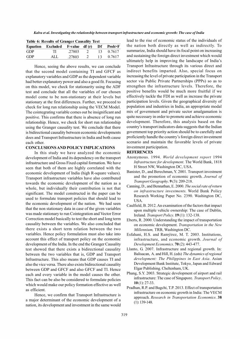
319
Hence, seeing the above results, we can concludethat the second model containing TI and GFCF asexplanatory variables and GDP as the dependent variablehad better explanatory power and also a good fit. Focusingon this model, we check for stationarity using the ADFtest and conclude that all the variables of our chosenmodel come to be non-stationary at their levels butstationary at the first differences. Further, we proceed tocheck for long run relationship using the VECM Model.The cointegrating variable comes out be insignificant andpositive. This confirms that there is absence of long runrelationship. Hence, we check for short run relationshipusing the Granger causality test. We conclude that thereis bidirectional causality between economic developmentsdoes and Transport Infrastructure in India and both causeeach other.CONCLUSIONS AND POLICY IMPLICATIONS
In this study we have analyzed the economicdevelopment of India and its dependency on the transportinfrastructure and Gross Fixed capital formation. We haveseen that both of them are highly correlated with theeconomic development of India (high R-square values).Transport infrastructure variables have also contributedtowards the economic development of the nation as awhole, but individually their contribution is not thatsignificant. The model constructed in the paper can beused to formulate transport policies that should lead tothe economic development of the nation. We had seenthat the non stationary data in case of the given variableswas made stationary to run Cointegration and Vector ErrorCorrection model basically to test the short and long termcausality between the variables. We also concluded thatthere exists a short term relation between the twovariables. Hence policy formulation must also take intoaccount this effect of transport policy on the economicdevelopment of the India. In the end the Granger Causalitytest showed that there exists a bidirectional causalitybetween the two variables that is, GDP and TransportInfrastructure. This also means that GDP causes TI andalso the vice versa. There also exists bidirectional causalitybetween GDP and GFCF and also GFCF and TI. Henceeach and every variable in the model causes the other.This fact can be also be considered to formulate policieswhich would make our policy formation effective as wellas efficient.
Hence, we confirm that Transport Infrastructure isa major determinant of the economic development of anation, its development and investment in the same would
lead to the rise of economic status of the individuals ofthe nation both directly as well as indirectly. Tosummarize, India should have its focal point on increasingand sustaining the foreign direct investment which wouldultimately help in improving the landscape of India’sTransport Infrastructure through its various direct andindirect benefits imparted. Also, special focus onincreasing the level of private participation in the Transportsector via Public Private Partnerships (PPPs) so as tostrengthen the infrastructure levels. Therefore, thepositive benefits would be much more fruitful if weeffectively tackle the FDI as well as increase the privateparticipation levels. Given the geographical diversity ofpopulation and industries in India, an appropriate modalmix of government and private sector amalgamation isquite necessary in order to promote and achieve economicdevelopment. Therefore, this analysis based on thecountry’s transport indicators data suggests that the Indiangovernment top priority action should be to carefully andproficiently handle the country’s foreign direct investmentscenario and maintain the favorable levels of privateinvestment participation.REFERENCESAnonymous. 1994. World development report 1994
Infrastructure for development. The World Bank, 1818H Street NW, Washington DC, USA.
Banister, D., and Berechman, Y. 2001. Transport investmentand the promotion of economic growth. Journal ofTransport Geography. 9 (3): 209-218.
Canning, D., and Bennathan, E. 2000. The social rate of returnon infrastructure investments. World Bank PolicyResearch Working Paper No. 2390. Washington DC,USA.
Caulfield, B. 2012. An examination of the factors that impactupon multiple vehicle ownership: The case of Dublin,Ireland. Transport Policy. 19 (1): 132-138.
Eberts, R. 2000. Understanding the impact of transportationon economic development. Transportation in the NewMillennium, TRB, Washington DC.
Esfahani, H.S. and Ramýìrez, M. T. 2003. Institutions,infrastructure, and economic growth. Journal ofDevelopment Economics. 70 (2): 443-477.
Llanto, G. 2007. Infrastructure and regional growth. In:Balisacan, A. and Hill, H. (eds) The dynamics of regionaldevelopment: The Philippines in East Asia. AsianDevelopment Bank Institute, Tokyo, Japan and EdwardElgar Publishing. Cheltenham, UK.
Phang, S.Y. 2003. Strategic development of airport and railinfrastructure: The case of Singapore. Transport Policy.10 (1): 27-33.
Pradhan, R.P. and Bagchi, T.P. 2013. Effect of transportationinfrastructure on economic growth in India: The VECMapproach. Research in Transportation Economics. 38(1): 139-148.
Kalra et al. Investigating the relationship between transport infrastructure and economic growth: The case of India
Table 6: Results of Granger Causality TestEquation Excluded F-value df (r) Df Prob>FGDP TI .27803 2 13 0.7617GDP ALL 2 0.7617

320
Indian J Econ Dev 12 (2): 2016 (April-June)
Sanchez Robles, B. 1998. Infrastructure investment andgrowth: Some empirical evidence. ContemporaryEconomic Policy. 16 (1): 98-108.
Shah, A. 1992. Dynamics of public infrastructure, industrialproductivity and profitability. The Review of Economicsand Statistics. 74 (1): 28-36.
Short, J., and Kopp, A. 2005. Transport infrastructure:Investment and planning. Policy and researchaspects. Transport Policy. 12 (4): 360-367.
Wang, E.C. 2002. Public infrastructure and economic growth:A new approach applied to East Asianeconomies. Journal of Policy Modeling. 24 (5): 411-435.

321
Indian Journal of Economics and DevelopmentVolume 12 No.(2): 321-326
April-June, 2016DOI: 10.5958/2322-0430.2016.00142.6
www.soed.in
Socio-Economic Factors Affecting Adoption Behaviour ofFarmers for Net-House Vegetable Cultivation in PunjabManjeet Kaur1*, M.K. Sekhon1, Amrit Kaur Mahal2, and Rakhi Arora1
1Department of Economics and Sociology, Punjab Agricultural University, Ludhiana 1410042Department of Mathematics, Statistics and Physics, Punjab Agricultural University, Ludhiana 141004
*Corresponding author’s email: [email protected]
Received: April 10, 2015 Accepted: June 06, 2016
ABSTRACTThis paper explores the impact of various socio-economic characteristics of farmers in adoption of net house vegetablecultivation. The study is based on the primary data collected from a sample of 120 farmers consisting of 60 net house and60 open field vegetable growers. The data were collected for the year 2011-12. Logistic Regression Model was used toempirically quantify the relative influence of various socio-economic variables in the adoption of net house cultivation.The socio-economic variables considered were age, family size, farm size, education, income, extension contacts andmembership of farmers’ professional societies. The analysis brought out that the income from other sources than cropincome, farmers having extension contacts and membership of professional societies significantly enhance the adoptionof net house technology.
KeywordsNet house vegetable cultivation, adoption behavior, logit model
JEL CodesO33, Q12, Q16
INTRODUCTIONIndia is the second largest producer of fruits and
vegetables in the world, next to China with an estimatedannual production of about 256.1 million tonnes from anarea of about 15.6 million hectares at an average yield of16.3 tonnes per hectare in 2014-15 (www.agricoop.nic.in)India’s share is about 10 per cent of the world output ofvegetables. However, its per capita per day availability iswell below the recommended level. The presentproduction is not sufficient to meet the requirement; thetarget can be achieved by bringing additional area undervegetable crops, using hybrid seeds, improved agrotechniques, perfection and promotion of protectedcultivation of vegetables. Fruits and vegetable cropsreceive considerably high quantity of pesticides, and witha cropped area of three per cent, these crops consume13 per cent of the total pesticides in the country (Nigamand Murthy, 2000). The effect of chemical and pesticideuse is more harmful in vegetables as compared to otherfood crops.
In Punjab state, vegetables occupied 1.92 lakh haarea and formed 2.5 per cent of total cropped area in thestate during 2012-13. Though vegetable farming seemsto be a good replacement for paddy-wheat monoculturebecause vegetable crops give high returns per unit areaas compared to rice wheat and being more labourintensive as compared to cereals , provide moreemployment opportunities for hired as well as familylabour (Bhatti and Singh, 1993; Kaur et al., 2001, andSekhon and Kaur, 2004). But farmers are not willing toleave paddy-wheat rotation because vegetable crops aremore prone to weather conditions and are risky (Kaur etal., 2005). The high-tech production of vegetables underprotected conditions is the recent development in thisfield.
Producing vegetables under net house structure hasseveral benefits including reduced pesticides use, offseason vegetable production, advancing maturity,increased productivity period and improved quality.Adoption of technological innovations in agriculture seems

322
Indian J Econ Dev 12 (2): 2016 (April-June)
to offer opportunities to increase production and incomesubstantially. But the introduction of many newtechnologies has met with only partial success, asmeasured by the observed rate of adoption (Feder etal.,1985). In the light of the facts mentioned above, thepresent study has been planned in the Punjab state withthe objectives:i) to analyse the influence of various socio-economic
factors of vegetable growers on the adoption behaviorof net house vegetable cultivation and
ii) to ascertain the opinion of non-adopter vegetablegrowers for not adopting net house technology forvegetable cultivators.
METHODOLOGYThe study is based on primary data collected from
vegetable growers of Punjab State. For the selection ofsample households cultivating vegetable under net house,a list of net house vegetable growers was obtained fromthe officials of Punjab State Farmers’ Commission, Mohali.As per the list the net house vegetable cultivators werethinly spread all over the state. The districts having highconcentration of net house users were selected. A sampleof 60 net house vegetable cultivators was selected from12 districts of Punjab. For comparison purpose an equalnumber of vegetable growers, cultivating vegetables inthe open field were also selected either from the samevillages or nearby villages. Thus, sample size comprisedof 120 vegetable growers consisting of 15 small, 20medium and 25 large net house vegetable cultivators; 23small, 18 medium and 19 large open field vegetablecultivators. The data on various socio-economiccharacteristics such as age, education, annual incomefrom agriculture, off-farm income, extension contacts,sources of information of new technology, membershipstatus of different farmers’ societies/clubs etc. werecollected from both categories of vegetable growers. Datawere collected during September 2012 to January 2013for the reference year 2011-12.
Simple averages and percentages were used to depictsocio-economic profile of sample households and opinionof farmers for non-adoption of net house vegetablecultivation.
Logistic Regression Model was used to empiricallyquantifying the relative influence of various socio-economic parameters in adoption of net house technologyin vegetable cultivation. The study has postulated thatthe probability of a farmer adopting net house technologydepends on socio-economic variables such as age,education, farm size, income from subsidiary occupations,number of earners in the family and extension contacts.The Index Variable Li indicating whether a farmer isadopting new technology has been expressed as a linearfunction of the independent variables. Thus, the logit
regression model has been specified as follows:Li=0+ 1X1+2X2 + 3X3+ 4X4+ 5X5+ 6X6+ 7X7 + Ui
X1 =Age of the head of the household (years)X2 = Family size (No.)X3 = Farm size (Acre)X4 = Education of head of the household (above secondary level =1; otherwise = 0)X5 = Off-farm income (`per annum)X6 = Extension contacts (If yes = 1; if no = 0)X7 = Membership of society (If yes=1, if no =0) = Constant1 to = Parameters to be estimated, andUi = Error term
RESULTS AND DISCUSSIONSocio-economic Characteristics of Farmers
The socio-economic characteristics of farmers havegreat bearing on adoption of new technologies/techniquesof production. Important socio-economic characteristicsof both categories of vegetable growers have beendepicted in Table 1. Among the sample household’smaximum concentration of farmers was in the age groupof 41-50 years among both categories of vegetablegrowers, the average age being 48 and 45 years in nethouse and open field vegetable cultivators respectively.Education-wise, the distribution of farmers showed thatthe net house vegetable growers were comparatively moreeducated, none of the farmer was illiterate among thiscategory whereas 15 per cent open field vegetable growerswere illiterate. Household’s in the category of educationalqualification of +2 and above were 43 percent and 28percent in case of net house vegetable growers and openfield vegetable growers respectively; farmers havingeducation up to graduation and post-graduation were moreamong net house vegetable growers. The average numberof years in the school were 11 and 9 in the case of nethouse and open field category households respectively.
The operational size of holding was 6.07 ha and5.06 ha in net house and open field vegetable cultivatorsrespectively. About 30 per cent of total cropped area wasunder vegetables in both the categories. Family size was5.95 and 6.75 members respectively. The average numberof members working in agriculture was higher in openfield category than net house vegetable cultivators. Thedependency ratio was also higher at 2.00 members inopen field category than net house vegetable cultivatorsat 1.90 members mainly because of large family size incase of the open field vegetable cultivators than theircounterpart net house vegetable growers. Family incomeduring the survey period was `959097 and `485426 fornet house and open field vegetable cultivators respectively.The farm income (crops+dairy) constituted about threeforth of family income in both the categories. The incomefrom net house vegetable cultivation formed 10.21 percent

323
of family income in case of net house vegetablecultivators.Membership of Farmer Societies/Clubs
The distribution of vegetable growers according tothe membership of different Societies/Clubs which showsthe progressive minds of farmers has been presented inTable 2. It is clear from the table that more number ofnet house vegetable growers were members of differentSocieties/Clubs than open field vegetable growers. Among
the net house vegetable cultivators, 30 percent of thefarmers were members of cooperative societies, whereasonly about 12 percent of open field vegetable cultivatorshave membership of cooperative societies. Twenty threepercent of net house vegetable cultivators were membersof Farmer’s Club PAU, whereas only about 2 percent ofopen field vegetable cultivators were members ofFarmer’s Club. Net house vegetable growers were alsothe members of other societies but the open field growers
Table 1: Important Socio-economic characteristics of sampled householdsSocio-economic parameters Net house cultivators Open field cultivators
Number Per cent Number Per cent1. Age (years)< 40 17 28.30 20 33.3041-50 23 38.30 18 30.00>50 20 33.40 22 36.70Average age (Years) 48 452. Education (No. of years in school)Illiterate - - 9 15.00Upto matric 35 58.30 34 56.7010+2 and above 26 43.30 17 28.30Average no of years in school 11 - 9 -3.Size of operation holdings (ha) 6.07 5.064.Family size and dependency ratio (No.)Family size 5.95 - 6.75 -No. of working members in family 3.1 - 3.39 -No of working members in agriculture 1.9 - 2 -Dependency ratio 1.92 - 1.995. Family income (` per annum)Income from crops 596294 62.17 355213 73.17Income from net house vegetable cultivation 97888 10.21 - -Total agricultural income 694182 72.38 355213 73.17Dairy 29319 3.05 35511 7.32Non-farm income 235596 24.57 94702 19.51Total family income/farm 959097 100.00 485426 100.00Figures within the parentheses are percentages to their respective total.
Table 2: Distribution of vegetable growers according to membership of societies/clubsNet house cultivators Open field cultivators
Particulars Number Percent* Number PercentCooperative Society 18 30.00 7 11.70Punjab Dairy Fed Association/Milkfed 10 16.70Agricultural Technology Management Agency 5 8.30Self help group 2 3.30Farmers’ Club PAU 14 23.30 1 1.70Net house vegetable growers Association/Societies 2 3.30Vegetable/horticulture growers Association 6 10.00Suraksha Agri. Rural Development Society 5 8.30*Multiple responseFigures within the parentheses are percentages to their respective total.
Kaur et al.: Socio-economic factors affecting adoption behaviour of farmers for net-house vegetable cultivation in Punjab
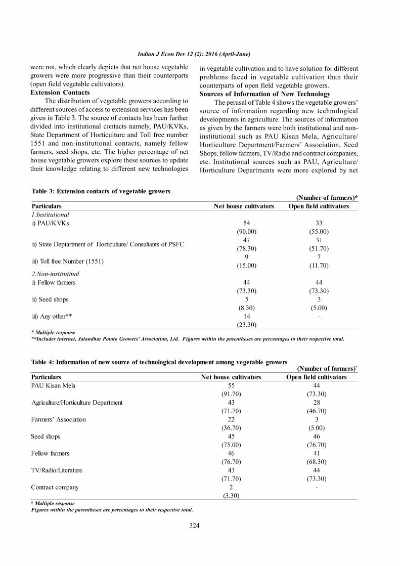
324
Indian J Econ Dev 12 (2): 2016 (April-June)
were not, which clearly depicts that net house vegetablegrowers were more progressive than their counterparts(open field vegetable cultivators).Extension Contacts
The distribution of vegetable growers according todifferent sources of access to extension services has beengiven in Table 3. The source of contacts has been furtherdivided into institutional contacts namely, PAU/KVKs,State Department of Horticulture and Toll free number1551 and non-institutional contacts, namely fellowfarmers, seed shops, etc. The higher percentage of nethouse vegetable growers explore these sources to updatetheir knowledge relating to different new technologies
in vegetable cultivation and to have solution for differentproblems faced in vegetable cultivation than theircounterparts of open field vegetable growers.Sources of Information of New Technology
The perusal of Table 4 shows the vegetable growers’source of information regarding new technologicaldevelopments in agriculture. The sources of informationas given by the farmers were both institutional and non-institutional such as PAU Kisan Mela, Agriculture/Horticulture Department/Farmers’ Association, SeedShops, fellow farmers, TV/Radio and contract companies,etc. Institutional sources such as PAU, Agriculture/Horticulture Departments were more explored by net
Table 3: Extension contacts of vegetable growers(Number of farmers)*
Particulars Net house cultivators Open field cultivators1.Institutionali) PAU/KVKs 54 33
(90.00) (55.00)
ii) State Deptartment of Horticulture/ Consultants of PSFC 47 31(78.30) (51.70)
iii) Toll free Number (1551) 9 7(15.00) (11.70)
2.Non-institutinali) Fellow farmers 44 44
(73.30) (73.30)ii) Seed shops 5 3
(8.30) (5.00)iii) Any other** 14 -
(23.30)* Multiple response**Includes internet, Jalandhar Potato Growers' Association, Ltd. Figures within the parentheses are percentages to their respective total.
Table 4: Information of new source of technological development among vegetable growers(Number of farmers)*
Particulars Net house cultivators Open field cultivatorsPAU Kisan Mela 55 44
(91.70) (73.30)Agriculture/Horticulture Department 43 28
(71.70) (46.70)Farmers’ Association 22 3
(36.70) (5.00)Seed shops 45 46
(75.00) (76.70)Fellow farmers 46 41
(76.70) (68.30)TV/Radio/Literature 43 44
(71.70) (73.30)Contract company 2 -
(3.30)* Multiple responseFigures within the parentheses are percentages to their respective total.

325
house vegetable growers and non-institutional sourcesare equally approached by both categories of farmers.
From the above discussion, it is concluded that thenet house vegetable growers were having comparativelylarge size of holdings, more educated had smaller familysize, consequently lower dependency ratio, higher socialstatus in terms of membership of various farmers’societies/clubs, had more extension contacts and moreprogressive in adoption of new technologies than theircounterparts of open field vegetable growers.Factors Affecting the Adoption Behaviour
A functional analysis using Logit Model was carriedout to identify the probability of dependence of adoptionof net house technology on various socio-economicparameters of the selected farmers. The parametersincluded were age, education, family size, farm size,income from other sources than crop income, extensioncontacts and membership of societies. The variables suchas income from other sources other than crop income,farmers having extension contacts and membership ofprofessional farmers societies enhance the probability ofadoption of the net house technology (Table 5). Theprobability of adoption of net house technology improvesby 50 per cent with farmers having income from sources
other than crop income. The probability of adoption hasincreased by five per cent with improvement of extensioncontacts and being membership of societies each. Thusoff-farm income, extension contacts and membership ofsociety has significant impact on the adoption of net housetechnology.Open Field Vegetable Cultivators’ Opinion for Non-adoption of Net House Technology
The information from farmers cultivating vegetablesin open field was sought for the non-adoption of net housetechnology. Various reasons were quoted by them, whichare presented in Table 6. One-fourth of sample households(25 percent) reported as no knowledge of this technologyas the reason of non-adoption followed by high investmentcost, low subsidy and lack of finance as the reason fornon-adoption of net house technology for vegetablecultivation. Lack of time and labour, lack of land, smallscale of operations of net house were the other reasonsmentioned by them.
Lack of electricity connection for agriculturepurpose and farm being at distant place from theresidence were the other reasons quoted by some of openfield vegetable cultivators for non-adoption of net housetechnology.
Table 5: Parameter estimates for Logit ModelVariables Coefficients 95% wald Confidence Limits Probability of adoption of NHInterceptAge 1.003 0.959 1.049 0.5007Family size 1.163 0.979 1.383 0.5376Farm size 1.010 0.985 1.035 0.5024Education 0.972 0.328 2.882 0.4929Income 1.000** 1.000 1.000 0.5000Extension contacts 0.056** 0.014 0.230 0.0530Membership of societies 0.059** 0.014 0.246 0.0557Logliklihood ratio test Chi-square=61.7436 Pr >chi sq. <0.0001**significant at 5 percent level of significance Pi <0.05: significant at 5% level of significanceNH: Net house
Kaur et al.: Socio-economic factors affecting adoption behaviour of farmers for net-house vegetable cultivation in Punjab
Table 6: Reasons quoted by open field vegetable cultivators for non-adoption of net house technologyReason of non-adoption of technology No. of farmers PercentLack of awareness 15 25Hesitation about its success 4 6.7High cost and less subsidy/lack of finance 13 21.7Lack of time and labour 12 20Lack of incentive price for net house vegetables 4 6.7Farm at far distance from village 3 5.1Lack of land/electric tube-well connection 4 6.7Meagre area covered by it 2 3.3Prone to high insects/pests attack 1 1.6Adopted but uprooted due to lack of electric tube-well 1 1.6Total 60 100
326
Indian J Econ Dev 12 (2): 2016 (April-June)
CONCLUSIONSThe two major findings emerged from the study.
Firstly, those farmers who were involved in groups/clubsor societies were showing more interest in adoption ofnet house and Secondly, farmers with sources of incomeother than crops favoured the adoption of net housetechnology. While introducing new technique/method orpractice in agriculture there is need to create awarenessamong the farmers. There are different ways to introducenew practices, the present study finds that farmers’ club/groups can play a pivotal role in influencing the behaviorof farmers towards use of net house for vegetablecultivation. Majority of the net house adopters weremembers of the farmers’ related societies in theirrespective areas. Secondly, the adoption of new practicesinvolved both production and market risks, which farmerswere unable to take without financial support. Toencourage the net house cultivation farmers should besupported by providing financial and institutional back-up.REFERENCESBhatti, J.P. and Singh, R.L. 1993. Change in the population of
labour force and land use in Himachal Pradesh: A strategyfor agricultural development in hilly area. The BiharJournal of Agricultural Marketing. 1: 329-338.
Feder, Jusc G.R.E and Zilberman, D. 1985. Adoption ofagricultural innovations in developing countries.Economic Development and Cultural Change. 33 (2):255-298.
Kaur, M., Kaur, M.K., and Rangi, P.S. 2001. Small farmers:Their problems and possibilities of development inPunjab state. Political Economy Journal of India. 10(1-2): 59-67.
Kaur, M., Singh, R., and Sekhon, M.K. 2005. Economicevaluation of contract farming system for snow-peascultivation in Punjab. Productivity. 46 (1): 142-145.
Nigam, G.L. and Murthy, K.S. 2000. An optimum use ofpesticides in integrated pest management technology.Pesticides Information. 25 (1): 6-9.
Sekhon, M.K and Kaur, M. 2004. Role of small farmers indiversification of Punjab agriculture with vegetables.Indian Journal of Agricultural Marketing. 18 (1): 80-88.
Webliographywww.agricoop.nic.in
327
Indian Journal of Economics and DevelopmentVolume 12 No. 2: 327-334
April-June, 2016DOI: 10.5958/2322-0430.2016.00143.8
www.soed.in
An Empirical Analysis of Pilgrimage Tourism in Jammu andKashmirRuhi Refath Aara*and Paramjeet Kaur Dhindhsa
Punjab School of Economics, Guru Nanak Dev University, Amritsar-143005 (Punjab)
*Corresponding author’s email: [email protected]
Received: September 22, 2015 Accepted: May 10, 2016
ABSTRACTThis study aims at to find out the factors which are purely responsible for the growth, development and sustainability ofTourism Industry of Jammu and Kashmir with special reference to Pilgrimage Tourism. Study uses both primary andsecondary data, consisting of 26 different categories of responses from the respondents. Principal Component and FactorAnalysis has been used to derive the important factors affecting the growth and development of the pilgrimage tourism.The empirical analysis reveals that eight factors came out to be significantly affecting the pilgrimage tourism in Jammuand Kashmir. Among them, provision of Private facilities came out to be the most significant followed by Public facilitiesand accommodation facilities. The other five factors which affecting Pilgrimage Tourism, directly or indirectly, wereMarket infrastructure, Hygiene and Banking infrastructure, Medical and Telecommunication infrastructure, Transportinfrastructure and Security and Information and Publicity. Furthermore, the study also shows that there is an urgent needfor well-planned strategy by all the stakeholders of the tourism industry of the state.
KeywordsTourism, pilgrimage tourism, factor analysis, Jammu and Kashmir, Amar-Nath Yatra
JEL CodesR42, Z12, Z30, Z32
INTRODUCTIONTourism has emerged as a key sector of the world
economy and has become a major sector toaccommodate large workforce globally. It has beenmaking a revolutionary and significant impact on the worldeconomic scenario. WTO states that tourism is, “Theactivity of the people who travel to places outside theircustomary surrounding and stay there, for leisure,business or other purpose, for no longer than one yearwithout interruption” (Bhatt and Badan, 1999). Themultifaceted nature of this industry makes it a catalyst toeconomic development and helps balanced regionaldevelopment. It is a low capital, labor intensive industrywith economic multiplier and offers opportunities to earnforeign exchange at low social cost. Tourism industryacts as a powerful agent of both economic and socialchange. It stimulates employment and investment,modifies economic structure and makes positive
contributions towards balance of payment (Anonymous,2015).
Tourism has now become a significant industry inIndia, contributing around 5.9 percent of the GrossDomestic Product (GDP) and providing employment toabout 41.8 million people (Sharma et al., 2012). As perthe World Travel and Tourism Council, the tourismindustry in India is likely to generate 121.4 billion of USdollars of economic activities by 2015 and Hospitalitysector has the potential to earn 24 billion US dollars offoreign exchange by 2015 (www.indiacore.com).Tourism today is the most vibrant tertiary activity and amulti-billion industry in India. Traditionally known for itshistorical and cultural dimensions, tourism today ishighlighted for its immense business opportunities (Patel,2012). In India Religion is a dominant motivation for traveland pilgrimage sites render them different from touristdestinations (Kaur, 2013). Travel for religious purpose

328
Indian J Econ Dev 12 (2): 2016 (April-June)
has been there form the most ancient times, particularly,all religions- Hinduism, Buddhism, Jainism, Islam andSikhism. The term “pilgrimage tourism” implies travel toa site or worship or a sacred place that has motivated byreligious motives. Conceptually it is not unlike recreationalor tourism movements as a form of short term migration.It is one of the most geographically significant forms ofreligious behavior. Pilgrimage tourism in India has beenpracticed since times immemorial. It is land of religiousand pilgrimage centers and is showing phenomenal growthin this direction (Chand, 2011) and (Gupta, 2007). It isregarded as the most suitable consideration for sustainabledevelopment of tourism in this subcontinent.Brief Review of Literature
There is good body of literature discussing aboutthe relation between tourism and pilgrimage on variedtheoretical grounds (MacCanell, 1976, Cohen, 1992,Smith, 1992, and Graburn, 2001). Pilgrimage tourism isbeing recognized as a prime industry in most parts of theworld. For the purpose of earning maximum foreignexchange. Pilgrimage tourism is playing a major role insocio-economic development. Tourism has been identifiedas the major export industry in the world (Anonymous,2014). The economic significance of pilgrimage tourismis very large, when measured against GDP and exports.And the social significance of pilgrimage tourismmeasured in terms of employment (especially unskilledlabor) is very large. A part from devotional aspect lookedat from the broader point of view, pilgrimage involvessightseeing, travelling, visiting different places and in somecases voyaging by air or sea, etc. and buying the localmemorabilia, almost everything a tourist does (Gupta,1999).
Given the importance and magnitude of pilgrimagetourism, the infrastructure and services at the pilgrimagesites needs to be developed in such a way that can bepositively sustained for the coming millenniums (Kumarand Singh, 2014). Kaul and Gupta (2009), stated that thebalance between sustainable development and pilgrimagetourism not only improve economic development but mustalso be synonyms with environmental, socio-culturalpreservation and protection in order to ensure a successfulpilgrimage tourism industry. Kumar and Singh (2014) isof the opinion that the pilgrimage destinations have enoughpotential to benchmark as a famous tourist spots. Gupta,(2007) highlighted that among various tourism forms,pilgrimage tourism can achieve the goal of sustainabilityeffectively as it is inherently having features such as lessburden on environment, local communities are involvedto a large extent, and very less cultural difference betweenguest and host as well. (Vijayanand, 2012), for manycountries in general and the least developed countries inparticular, pilgrimage tourism is a sector in which they
have comparative advantages, if not competitive for whichthey can efficiently convert domestic tourism into foreignexchange. Tourism is an effective means of earningforeign exchange and providing tremendous employmentopportunities beside, guiding modernization ofinfrastructure and acting as a catalyst in the growth of allsectors of economy. In simple words tourism meanstransfer of wealth from one country to other (Kaur, 2013).
The above literature though significant enough todeliver the behavior of tourism industry of India. However,lack a very important aspect of quantifying the strengthand the factors which may be responsible for the growthand sustainability of the industry directly or indirectly.Further there is no study in the literature, to the best ofour knowledge, for sub national level (like state of Jammuand Kashmir). This study aims at examining the growthand potential of Pilgrimage Tourism in Jammu andKashmir, with special reference to Amar-Nath shrine. Thestudy also attempts to measure the satisfaction level ofpilgrims with respect to the various tourism services duringAmar-Nath Yatra. The main purpose of performing thisanalysis is that it will highlight the factors which are purelyresponsible for growth and sustainability of tourismindustry of Jammu and Kashmir. The rest of the paper issequenced as: Section 3 provides a brief description aboutthe data. Section 4 deals with detailed description aboutthe methodology used. Section 5 provides results anddiscussion. Section 6 concludes the paper and providespolicy implications.DATAAND METHODOLOGY
The study is based on both primary and secondarydata. Secondary data have been taken from variouspublished and unpublished records of Ministry of Tourism,Government of India, Government of Jammu andKashmir, Digest of Statistics, Directorate of Economicsand Statistics Planning Jammu and Kashmir, Directorateof Tourism Department Jammu and Kashmir. Inadequacyin the secondary data has necessitated the collection ofadditional information directly from the pilgrims/tourists.Accordingly a pretested questionnaire was administeredpersonally and 100 respondents were selected on the basesof random sampling technique. The questionnaire wasdesigned to understand the difficulties, expectations andneeds of the tourists in connection with transportation,boarding, lodging and shopping services and behavior ofthe local public. The data collected has been compiled,tabulated and analyzed with the help of various statisticaltechniques.
In order to understand and measure the satisfactionlevel of pilgrims/tourists during Amar-Nath Yatra, in Jammuand Kashmir, Factor Analysis technique has been appliedon a series of 26 statements showing the level ofagreement/disagreement with the availability of various

329
Arra and Dhindsha: An empirical analysis of pilgrimage ourism in Jammu and Kashmir
services/facilities available at the pilgrimage/religiousplace. Factor analysis is generally used in a regression toinvestigate dimensionality between the linearly related andunobservable variables/factors (Harman, 1967). It has apower to reduce the redundancy of the data set to aneffective application without losing the information ofspecification. The basic function used in multifactor model
with set of variables qiy 1 , factors n
k 1 and residuals qi 1
for a particular specification can be represented as:
)1....(
.........
..............
,,,1,2,02,
2,,,21,2,202,
1,,1,1,101,
qinknnkni
inknki
inknki
y
yy
Where: 0 is an intercept, s represent the factor
loadings, s are factor values and qi , is stochastic errorterm with zero mean and constant variance. The abovemodel can be represented in simplest form of Matrixnotation.
)2(.......εηββγ iii0i ++=
)3(.......
.
.
.
............
..........
.
.
.
,...
,
1,
,
1,
,1,
,1,
,0
1,01,
ni
i
ni
i
nmm
nii
n
i
nyi
y
Where 0 is the vector of intercepts, 1 is thematrix of factor loadings, (i 1. . . . . .k n) is the matrix offactors (variance and covariance) and i is the matrix ofresiduals. The above equations helps to identify the factorsto be analyzed and suggests the true factor value for eachcategory. In order to have better understanding about thefactors, the loadings have been rotated using Kaiser’sRaw Varimax Criterion (Kaiser, 1958). All the factors whichturned out to be significant have been grouped in theirrespective group and interpreted accordingly.EMPIRICAL RESULTSOver View of Jammu and Kashmir Tourism-Pilgrimage Tourism
The Jammu and Kashmir is the one of the northernstates of India with huge potential of attracting touristsfrom within and across the globe probably due to its ethnicbeauty. Although it is not so attractive on religious basisit still has some renowned pilgrimages and shrines within.Jammu and Kashmir is a state that is considered a holyplace by people of all the religions and gets the maximum
share of tourism from pilgrimage tourism. Jammu andKashmir has been called paradise on earth by, as it oftenhas been by its lovers, it is not for its natural beautyalone; for the shrines have preserved a communion faithtranscending all other barriers. Of equal importance tothe travelers are the valley’s many monuments reflectingthe glory of mankind. Legends and history haveintertwined to give its shrines an evocative embrace thatbrings to life the richness of the state’s spiritual culture.
The State of Jammu and Kashmir has been a seat ofreference to all major religions of the world. This state isfull of holy sites and most of these sites are located inbetween scenic surroundings of great Himalayas. Thisaspect is responsible for attracting large number oftourists every year, which has ultimately led to boom inthe tourism industry of the state. This way, tourists notonly just explore the spectacular landscapes but theopportunity of worshipping at the respective religiousshrines. It has various religious centers which are justmarvel creations. Visiting Hari Parbat Pilgrim Centerwhere a Temple (Hindu worship site), a Gurudwara (Sikhworship site) and a Mosque (Muslim worship site) standside by side gives a feeling of pure brotherhood in betweenof major religions of the state. It has various pilgrimdestinations for Hindus, Muslims and Buddhists. The veryfamous Sri Amar-Nath Shrine is one of them. It is themost valued and sanctified of Hindu pilgrimage site wherethousands of devotees pay homage every year.Sterilized Facts about Tourism industry of the State-Pilgrimage Tourism
Amar Nath pilgrimage is a huge attraction for touristsand pilgrims in Jammu and Kashmir as reported by (Dograand Gupta, 2012). Amar-Nath shrine is situated in anarrow gorge at the farther end of the Kashmir(Pahalgam). Every year thousands of Hindu pilgrimsgather in the month of Shraven (July-August) to offerprayers to this incredible shrine. Entrance to the shrine isregulated as Darshan (site seeing) mostly controlled byPandits (priests).
The results presented in Table 1 show that the inflowof devotes visiting the holy shrine have been continuouslyincreasing over the period of time. No doubt there arefluctuations in the devotees’ influx but on the whole therehas been a continuous increase in pilgrims visiting theshrine. In 1984 only 9483 pilgrims visited the shrine andits number has increased to 96055 pilgrims in 1988.However, the number starts declining after 1990 due tothe fact that certain militant out-fits had imposed a banon the movement of tourist traffic visiting Amar-NathShrine; hence there was sharp decline in the number ofpilgrims visiting the shrine during 1990’s. But after 1995the inflow of pilgrims picked up and this might be due tothe efforts of the government put forward to provide

330
Indian J Econ Dev 12 (2): 2016 (April-June)
KashmirThe main purpose of performing factor analysis is
that it will highlight the factors which are purelyresponsible for growth and sustainability of tourismindustry of Jammu and Kashmir. The application thismethod helped in finding out the relative significance ofthe factors that determine the satisfaction level of therespondents for the pilgrimage tourism in the state. Inorder to find out relevant factors which are responsiblefor the growth and development of the tourism industryof the state a simple factor model described in section 4and principle component analysis (PCA) has been usedfor extracting factors. The PCA has been computed anddetermined by Eigen vectors and their values from acovariance matrix. This matrix is being used to understandthe variations in dimensions with respect to each otherfrom the estimated mean. The number of factors to beretained was based on the Eigen Values and percentageof variance accounted by the same. The general agreementabout the selection of factors based on Eigen values isthat only those factors can be traced out and used forfurther analysis whose Eigen values turn out to be greaterthan 1. Following this procedure the results shows thatonly eight factors could be extracted which explained52.94 percent of total variance. All factors were seen tobe highly significant. Hence all the eight factors werepresented for the analysis. The number of factors andtheir respective explained variance is reported in Table 2.are purely responsible for determining the relationship.
In order to have better understanding about thefactors, the loadings have been rotated using Kaiser’sRaw Varimax criterion (1958). All the factors which turnedout to be significant have been grouped in their respectivegroups and interpreted accordingly in the next section.The results were obtained through an iteration processwhich converged in only 20 replications reflecting a highreliability of factors chosen. The result of rotational matrixfor over all sample are reported in Table 3. The resultsclearly shows that the factors are highly relevant and are
Table 1: Year-wise flow of yatries/visitors to Jammu andKashmir
(No.)Year No. of yatries/visitors Percentage change1984 9483 -1985 42000 342.961986 51000 21.431987 52000 1.961988 96055 -84.721989 95238 -0.851990 4824 -94.931991 15599 223.361992 54638 250.271993 56000 2.491994 37000 -33.931995 60000 62.101996 120000 100.001997 79035 -34.101998 149920 89.601999 114366 -23.702000 173334 51.502001 119037 -31.302002 110793 -6.922003 145772 92.392004 171811 17.862005 388000 125.822006 265000 -31.702007 213565 -19.402008 498198 133.272009 373419 -25.042010 458212 22.702011 635660 38.72Source: Directorate of Tourism, Government of Jammu and Kashmir
various types of facilities and amenities to the pilgrimsfor their safe and comfortable arrivals. Because of allthese efforts the devotees visiting holy shrine, which haddeclined to 4829 in 1990, again started increasing andwent up to 635660 in 2011.Factor Analysis-Pilgrimage Tourism of Jammu and
Table 2: Extracted number of factors using PCA and factor modelComponent Initial Eigen values Extraction Sums of Squared Loadings Rotation Sums of Squared
LoadingsTotal Percentage
of VarianceCumulativePercentage
Total Percentageof Variance
CumulativePercentage
Total Percentageof Variance
CumulativePercentage
1 2.36 9.077 9.077 2.36 9.077 9.077 1.995 7.672 7.6722 1.964 7.554 16.631 1.964 7.554 16.631 1.851 7.12 14.7923 1.868 7.186 23.817 1.868 7.186 23.817 1.766 6.794 21.5854 1.842 7.084 30.901 1.842 7.084 30.901 1.71 6.579 28.1645 1.63 6.271 37.172 1.63 6.271 37.172 1.71 6.576 34.746 1.524 5.86 43.031 1.524 5.86 43.031 1.651 6.35 41.097 1.311 5.043 48.074 1.311 5.043 48.074 1.578 6.07 47.168 1.266 4.868 52.942 1.266 4.868 52.942 1.503 5.782 52.942

331
explaining significant portion of the relation. The resultsfurther confirms the factor loadings of the factors chosen.
Identifying the variables that have large loading onthe same factor facilitates naming and interpretations. Thenames of the factors, the statement labels’ and factorloadings have been summarized in the Table 4.Private Facilities (F1): This has emerged as the mostimportant factor explaining 9.007 percent of total variance.Three out of 26 statements load on to this factor. Highestloading is for the statement ‘private sector should be giventhe job to promote religious tourism in Jammu and Kashmir(0.757), followed by Cloak room facility and securityarrangements at the temple are satisfactory (0.599) andClean drinking water facilities are adequate on the wayand at the religious place (0.59). The respondents feelthat there is a need for more improved clean drinkingwater facilities on the way and at the religious place andproper cloak room facilities and security arrangement atthe temple. Most of the respondents state that the facilitiesprovided by the state government are somehowsatisfactory, but as the pilgrim’s traffic increases, therebecomes the shortage of these necessary facilities. So
this factor gives the direct policy implication that privatesector investment should be encouraged to develop thetourism infrastructure.Public Facilities (F2): This factor comprises of threestatements and it accounts for 7.554 percent of totalvariance. Highest loading in this factor is for the statement‘govt. provide adequate facilities on the way of the shrine(0.822), followed by ‘well connectivity of this place toyour place (0.715) and ‘food facilities are adequate at thereligious place (0.614). The responses regarding the firststatement of this factor was not much satisfactorybecause as per their opinion, which stated that govt. istrying its best in providing the basic necessities /facilitiesto the tourists/pilgrims but there always lies a gap betweenthe demand and supply.Accommodation Facilities (F3): The three statementsthat load into this factor explain 7.186 percent of thetotal variance. Highest loading in this factor is for thestatement ‘Simple but clean accommodation with propersanitation and hygiene is available in the city at reasonablerates (0.75), followed by ‘Adequate accommodationfacilities are available there on the way to the religious
Arra and Dhindsha: An empirical analysis of pilgrimage ourism in Jammu and Kashmir
Table 3: Extracted factors with rotational matrixVariables Components / Factors
F1 F2 F3 F4 F5 F6 F7 F8X19 0.757X20 0.599X09 0.59X08X18 0.82X02 0.75X07 0.64X24X14 0.75X16 0.641X04 0.531X21 0.633X13 0.63X12 0.54X06 0.671X23 0.555X05X03X25X26 0.712X11 0.558X10 0.555X17 0.726X01 0.552X15 0.644X22 0.522

332
Indian J Econ Dev 12 (2): 2016 (April-June)
place (0.641) and the behavior of the locals towardstourists is good. The third statement, though not directlyrelating to this factor is also included in it. But theresponses regarding this statement, state that pilgrimsare highly satisfied with the behavior of locals, which isthe essential condition to stay in other culture and society.This factor also calculates that there is a great need toimprove the accommodation facilities mostly in the peakdays of the Amar-Nath Yatra. Because during these daysthe pilgrims/tourists flow increase very fast, this led to agap between the demand for and supply of adequateaccommodation facilities.Market Infrastructure (F4): This factor was found tobe significant, and explained 7.084 percent of totalvariance. It reveals that ‘There is need to open moreshopping centers of the state Art and Craft and otherreputed items around the place (-0.633), followed byShopkeepers around the religious place don’t cheat thetourists (0.63) and arrangement for Prasad and otherofferings for prayers are good (0.54). This factor clearlyindicates that there is ample scope for the opening ofnew shopping centers of state Art and Craft and other
reputed items around the place. And there is also a needto improve the services through light and sound programswhich will definitely motivate the respondents to repeattheir visit in the state.Hygiene and Banking Infrastructure (F5): The fifthfactor explains 6.271 percent of total variance. Highloading for the statement ‘Toilets and bathrooms aresufficient in number in relation to pilgrim traffic (0.671)followed by ‘Banking facilities are adequate at this place(0.555). The respondents do not much appreciatesufficient toilets and bathroom facilities in relation topilgrim traffic. Therefore this factor calls for strengtheningof various facilities and services for tourists and suggestspromoting and modernizing banking services around thereligious places.Medical and Telecommunication Infrastructure (F6):This factor which accounts for the 5.86 percent of totalvariance states that pilgrims feel inadequatetelecommunication facilities at the tourist destination(0.712). Most of the respondents were highly unsatisfiedwith the telecommunication facilities. They claim that theirown mobile number does not work there and they are
Table 4: Naming of factors (over all sample)Factors Name of Dimension Label Statements/ (Factor Loading)F1 Private Facilities X19 Private sector should be given the job to promote religious tourism in the State of
Jammu and Kashmir.X20 Cloak room facility and security arrangements at the temple are satisfactory.X21 Clean drinking water facilities are adequate on the way and at the religious place.
F2 Public facilities X18 Govt. provides adequate facilities on the way of the shrine.X01 Well connectivity of this place with your place.X06 Food facilities are adequate at the religious place.
F3 AccommodationFacilities
X14 Simple but clean accommodation with proper sanitation and hygiene is available inthe city at reasonable rates.
X16 Adequate accommodation facilities are available there on the way to the religiousplace.
X04 The behavior of locals towards tourists is good.F4 Market Infrastructure X21 There is need to open more shopping centers of the state Art and Craft and other
reputed items around the place.X13 Shopkeepers around the religious place don’t cheat the tourists.X12 Arrangement for Prasad and other offerings for prayers are good.
F5 Hygiene and BankingInfrastructure
X06 Toilets and bathrooms are sufficient in number in relation to pilgrim traffic.X23 Banking facilities are adequate are there at this place
F6 Medical andTelecommunicationInfrastructure
X26 Inadequate telecommunication facilities are there at this placeX11 Adequate medical facilities are available on the way and at the religious placeX10 Fresh and hygienic food at langar (Junction) is appreciable.
F7 TransportInfrastructure andSecurity
X17 Adequate transport facilities are available to reach the base-camp
X014 There is a good feeling of safety at this religious place.
F8 Information andPublicity
X15 Information centers here provide relevant information relating the religious place.X22 Government. Publicity regarding pilgrimage tourism is adequate.

333
not allowed to get new SIM card from the statetelecommunication authorities. They are satisfied withthe medical facilities provided by the State governmenton the way and at the base-camp and also appreciatedthe fresh and hygienic food at langar (food Junction).Transport infrastructure and Security (F7): This factoraccounts 5.043 percent of total variance. Which statesthat pilgrims feel ‘adequate transport facilities are availableto reach the base-camp (0.726), but they did not feel‘There a good feeling of safety at this religious place (-0.552). It was evident from the responses of the pilgrimsthat they feel insecure in the state and at the religiousplace too. They appreciated the security facilities providedby the government of Jammu and Kashmir, but still theyare having the serious threat in their hearts and minds,due to the past militant kidnapping events regarding theyatries/tourist in the state. Therefore this factor focusestowards the light and sound programs/counseling isneeded to make the brainwash of this threat in the touristsas a whole by the State government through print andelectronic media.Information and Publicity (F8): In this last factor twostatements load which explains 4.868 percent of totalvariance. Highest loading in this factor is for ‘informationcenters which provide relevant information relating tothe religious place (0.644) followed by ‘government.Publicity regarding pilgrimage tourism is adequate (0.522).Which suggests that respondents are satisfied withrespect to information centers which provide relevantinformation to the pilgrims, but they are not much satisfiedwith the government publicity regarding pilgrimagetourism of the state. This factor gives a direct policyimplication that high level of promotion and publicity bythe state government is required to increase the pilgrims/tourists flow in the state.
Results of the factor analysis reveal that factor 1has emerged as the most important factor which presentsthe direct policy implications that ‘private sectorinvestment should be encouraged to develop tourisminfrastructure and tourism should be extensivelypropagated’. Factor 2 was defined as public facilities,which reveals that proper, improved and sufficient basicfacilities should be developed. For the tourists/pilgrimsthe availability of basic facilities and dispensation ofservices are of utmost importance. Factor 3 reveals theadequate accommodation facilities, which need to bedeveloped and improved so that the gap between supplyand demand should be bridged. Factor 4 presents mixedfeelings of tourists while shopping and staying at thereligious place. Pilgrims rued that lack of shopping centersof the state Art and craft. Factor 5 calls for thestrengthening of the tourist information services andsuggests promoting and modernizing banking services
around the religious place. Factor 6 reveals that thetelecommunication facilities should be improved. Factor7 suggests that light and sound programs by thegovernment authorities should be used to ensure thetourists/pilgrims a safe and happy tour in the state. Factor8 also suggests better publicity and information of allother tourist destinations through print and electroniccommunication. Besides all, the tourists have been foundto be expecting pro-active role being played by theGovernment in providing customer services includingmedical, banking, shopping and civic amenities includingroad signs and indications, information services,cleanliness of the surroundings of the shrine, transportfacilities, ample inexpensive accommodation and eatingjunctions etc.CONCLUSIONS
In conclusion, it may be re-emphasized that theconcerned religious bodies, government, NGO’s and othertourism stakeholders should make concrete efforts toprofessionally promote and support programs tostrengthen various services and facilities available for thepilgrims/tourists. The role of government lies in creatinga policy environment, in the formulation and enforcementof rules and regulations, in providing financial incentivesand infrastructural support in areas such as humanresource development and in the promotion and marketingof tourism, both domestically and internationally.SUGGESTIONSAND POLICY IMPLICATIONS
An effective pilgrimage tourism promotion strategyshould strongly focus on promoting and attracting theflow of domestic tourists from across different parts ofthe country. Since the analysis also revealed that Indiandomestic tourists particularly belong to affluent classes,visit other places primarily with religious motive. Thus adirect policy implication that a ‘tourism promotion policymust target rich domestic Indian tourists, who are keento visit for religious purposes is the need of hour. At thesame time, foreign tourists can be profitably targetedkeeping into consideration their ‘holidaying motive.
There is a strong need to construct pavilions, likemalls, containing shops and sale outlets for specific itemssuch as, pavilion for state Art and Craft, pavilion ofreligious items, folk items and pavilion for food and soon, so that the pilgrim’s desire for specific items can besatisfied within one enclosure. In addition, there is a strongneed to refurbish and expand government emporiumsselling diversified traditional culture items of Kashmir atfixed prices.
The Government of Jammu and Kashmir shouldorganize youth and cultural exchange programs for thedomestic tourists from neighboring states. One maysuggest a joint regional advertisement and publicity’ policywith a view to promote travel to the region.
Arra and Dhindsha: An empirical analysis of pilgrimage ourism in Jammu and Kashmir

334
Indian J Econ Dev 12 (2): 2016 (April-June)
Integration of excursion outings with religioustourism and to develop and professionally manage scenicpicnic of religious shrines. Hence, the promotional strategydiversifying reasons to visit’ can be adopted by linkingsacred sites with other attractions/motivators and torevalorize the holy place through its cultural identities.
Proper information including publicity of the placesof pilgrimage; public tourist information center; roadsignboards, and road maps, published tourism informationliterature in different languages strongly need to beaugmented. As the floodgates of the tourism sector havebeen opened, the opportunities, therefore, provided canbe profitably tapped only if thrust to increase inflow oftourists on one side is coupled with adequacy ofinfrastructure facilities available. As the present studyreports gross dissatisfaction with respect to banking,communication and other facilities available. Therefore,physical infrastructure and other infrastructure services,including elevated roads, traffic management, state ofart, banking facilities, mobile dispensaries, generalcleanliness of the places of stay and food and cateringservices need to be upgraded.
Public–private sector partnership is now witnessedin the development of infrastructure services for primereligious destinations. Such partnerships should also beundertaken for other important destinations as well. Theprivate sector as it is by the motive of profit, has theadvantage in providing the local development.
Adequate promotion of religious destinations ispossible if the associated management bodies tie-up withtour and travel operators who can importantly serve topromote religious destinations. They can serve thetourists/pilgrims by offering a suitable package as wellas impart required information, thus facilitating touristtravel and visit.REFERENCESAnonymous. 2014. World Tourism Organization. 2014. News
from the World Tourism Organization. Madrid, SpainBhatt, H. and Badan, B.S. 1999. Cultural tourism. Crescent
Publishing Corporation, New Delhi.Chand, M. 2011. Understanding religious tourism
motivations in India: An empirical investigationreligious tourism in Asia and the Pacific. UNWTOPublication. Madrid, Spain: 313-328.
Cohen, E. 1992. Pilgrimage and tourism: Convergence and
divergence. In: Morinis, A. (ed.) Sacred journeys: Theanthropology of pilgrimage. Greenwood Press, SantaBarbara, California, USA.
Dogra, R. and Gupta, A. 2012. Barriers to communityparticipation in tourism development empirical evidencefrom a rural destination. South Asian Journal of Tourismand Heritage. 1: 129-142.
Graburn, N.H. 2001. Secular ritual: A general theory of tourism.In: Smith, V.L. and Brent, M. (eds) Hosts and guestsrevisited: Tourism issues of 21st Century, CognizantCommunication Corporation, New York, USA.
Gupta, B. 2007. Pilgrimage tourism: A resource forsustainable tourism development. Anmol Publication,New Delhi: 220-226
Gupta, V. 1999. Sustainable tourism: Learning from Indianreligious traditions. International Journal ofContemporary Hospitality Management. 11: 91-95.
Harman, H.H. 1967. Modern factor analysis. University ofChicago Press, Chicago, USA.
Kaiser, H.F. 1958. The varimax criterion for analytic rotationin factor analysis. Psychometrica. 23. 187-200.
Kaul, H and Gupta, S. 2009. Sustainable tourism in India.Worldwide Hospitality and Tourism Themes. 1: 12-18.
Kaur, S. 2013. Tourism in Jammu and Kashmir with specialreference to Shri Mata Vaishno Devi. SIT Journal ofManagement. 3: 147-156.
Kumar, R.B. and Singh, L. 2014. Pilgrimage tourism inKurukshetra (Haryana): A sustainable developmentapproach. African Journal of Hospitality, Tourism andleisure. 3: 1-13.
MacCannell, D. 1976. The tourist: A new theory of leisureclass. Shocklen Books, New York.
Patel, R. 2012. Indian tourism industry- Progress and emergingissues. Arth Prabhand: A Journal of Economics andManagement (APJEM). 1: 1-10.
Sharma, A., Johri, A., and Chauhan A. 2012. FDI: Aninstrument of economic growth and development intourism industry. International Journal of Scientific andResearch Publication. 2 (10):1-6.
Smith, V. 1992. The quest in guest. Annals of TourismResearch. 19: 1-17.
Vijayanand, S. 2012. Socio-economic impacts in pilgrimagetourism. International Journal of MultidisciplinaryResearch. 2: 329-343.
Webliographywww.indiacore.com/tourism.html.

335
Indian Journal of Economics and DevelopmentVolume 12 No.2: 335-340
April-June, 2016DOI: 10.5958/2322-0430.2016.00144.X
www.soed.in
Economic Analysis of Milk Production among Small holderDairy Farmers in Punjab: A Case Study of Amritsar districtKashish*, Manjeet Kaur1, M.K. Sekhon1, and Vikrant Dhawan2
1Department of Economics and Sociology, Punjab Agricultural University, Ludhiana-1410042Department of Agronomy, Punjab Agricultural University, Ludhiana-141004
*Corresponding author’s email: [email protected]
Received: April 15, 2015 Accepted: April 20, 2016
ABSTRACTThe present study analyzed economics of milk production among small holder dairy farmers in Punjab. Amritsar districtwas selected purposively because the average milk production was quiet high in the district than state average and haswell developed milk cooperative societies. A sample of 80 dairy farmers consisting of 20 dairy farmers each from landless(LL), marginal (MR), small (SM) and other (OT) categories were selected from two blocks and four villages of Amritsardistrict. The average herd size was 6.35, 7.70, 9.40 and 10.05 dairy animals for LL, MR, SM and OT dairy farmers,respectively. The total variable cost was `145948.90, `170122.85, `200487.20 and `204122.60 for LL, MR, SM and OTdairy farmers, respectively. The average variable cost was to the tune of `180762.60. Feed and fodder cost was accountedfor 83.84 per cent out of the total variable cost. The total fixed cost accounted was `32733.5, `37537.59, `42640.5 and`46723.75 for LL, MR, SM and OT dairy farmers, respectively. Gross income from dairying was accounted to be `306946.80for LL, `397644.90 for MR farmers, `458120.60 for SM and `511401.50 for OT dairy farmers, respectively. The cost andincome had direct relationship with herd size for different categories of dairy farmers. To estimate the resources useefficiency in milk production, Cobb Douglas Production Function was used. The variables included in regression modelwere green fodder, dry fodder, concentrates, labour hours and veterinary and insemination charges considered asindependent variables and milk production per farm per day as dependent variable. The coefficient of multiple determination(R2) was 0.80 and indicating that about 80 per cent of total variations in milk productivity were explained by thevariables included in the selected regression model. The coefficients of dry fodder and concentrates were positive andsignificant indicating increase in feed and fodder inputs will increase the milk productivity.
KeywordsResource use efficiency, economic analysis, milk production.
JEL CodesC81, D57, R15INTRODUCTION
The prosperity of rural economy is closely linked toagriculture and allied activities (Bhasin, 2009). Thelivestock enterprise is adequately combined with cropenterprise by farmers of dry land region to overcomerisk (Anbukkani, 2015). Livestock production have beenviewed by planners and policy makers as an effectiveinstrument of social and economic change in the ruralareas, as they provide employment to the weaker sectionsand thereby help them in augmenting their incomes(Manhas, 2015). Dairying is an important segment oflivestock sector and is being considered as one of theviable options for diversifying the agricultural economy.
This sector provides 15-40 per cent income to nearly 70per cent of rural households. Dairying provides a regularsupplementary income and employment not only tomillions of producers in the rural areas but also to verylarge number of people engaged in secondary and tertiarybusiness related to livestock business and importantoccupation and a source of family income for largenumber of women in the village. It employs two thirdfemale work force (Kumar et al., 2010). Mostly 70 percent of milk was produced by small holder dairy farmersso there is need to increase the productivity of milk tomeet the increasing demand by providing some benefitsin the form of wages and subsidies to small farmers

336
Indian J Econ Dev 12 (2): 2016 (April-June)
(Kashish et al., 2014). Misra and Pal (2003) reportedthat 25% of the total earnings of villagers come fromdairying as a subsidiary activity of crop livestockintegration in rural area. The cost and return structure ofdairying is an important aspect for producers andconsumers to get better remunerative prices for milk saleand purchasing price by consumers at reasonable andcheaper rates (Bharti et al., 2015). The milk productionis influenced by various factors like quantity and qualityof feeds and fodders fed, order of lactation, stage oflactation, herd size, labour use etc. Hence there is needfor selection of suitable variables to study the milkproduction. The primary concern was regardingmaximum output of milk with minimum use of inputs.The feed cost was the major component and accountedfor 64 percent in Andhra Pradesh, 72 percent in TamilNadu and 74 percent in Karnataka (Reddy et al., 2004).In the economics of milk production among the variablefeeds, the cost of concentrates constitutes more thanone-third of the feed cost (Goswami and Rao, 1992 andKumar and Balishter, 1996). Resource use efficiencycomprised the distribution of a given amount of scarefactor among the set of alternatives in the production soas to maximize the profit (Kumar et al., 2000). Anempirical assessment of determinants of milk productionand resource use efficiency are important for planning,projecting and formulating dairy development policies ina particular region (Meena et al., 2012). The input-outputrelationship in milk production and resource use efficiencyhave been studied by several researchers in the variousparts of the country and found different for differentareas depending upon the type of milch animals and themilk production technology an increase in the level ofthis input demonstrated an increase in the production. Inthis context, the present study in-depth was undertakento study economics of milk production and resource useefficiency in milk production among different categoriesof dairy farmers.DATA AND METHODOLOGY
The study was based on primary data collected fromdairy farmers in the year 2013-14. For the selection ofsample households multistage random sampling techniquewas used. Amritsar district was selected at the first stageof sampling having higher milk productivity than the stateaverage and well established milk cooperative structure.In the second and third stage of sampling two blocksand two villages from each block were randomly selected.In the fourth stage of sampling, a list of all the dairy farmhouseholds from all the four villages were prepared andfarmers were categorized in to landless farmers (havingno land), marginal farmers (< 1 ha), small farmers (1-2ha) and other dairy farmers (> 2 ha). At the last stage ofsampling five dairy farm households from each category
were selected from each selected villages. Thus a sampleof 20 dairy farmers of each size category of landless(LL), marginal (MR), small (SM) and other (OT) wasselected making a sample of 80 dairy farm householdsfrom the selected categories.Analytical Techniques
Tabular analysis was employed to work out the coststructure and returns from dairy farming. To examinethe resource use efficiency multiple regression analysiswas carried out and log linear was selected on the basisof goodness of fit two models were tried as under:
Cob-Douglas functionY=b0X1
b1X2b2X3
b3X4b4X5
b5+U Log Y= b0 + b1 log X1 + b2 log X2 + b3 log X3 + B4 log
X4 + B5 log X5 + log D1 + log D2 + log D3 +UWhere,
Y= Milk production (litres/animal/day)b0= InterceptX1= Green fodder (kg/animal/day)X2 = Dry fodder (kg/animal/day)X3 = Concentrates (kg/animal/day)X4 = Labour employed (hours/animal/day)X5 = Veterinary charges (`/animal/day)D1 = Dummy variable (D1 for LL = 1 and for MR, SM and OT = 0)D2 = Dummy variable (D2 for MR = 1 and for OT, SM and LL = 0)D3 = Dummy variable (D3 for SM = 1 and for MR, OT and LL = 0)U = Error term
RESULTSAND DISCUSSIONImportant characteristics of sample dairy farmers
Before discussing the economics and resource useefficiency in milk production brief description of socioeconomic profile of sample households has been presentedin Table 1.The operational size of holding of MR, SMand OT dairy farmers was 0.65, 1.75 and 3.08 ha,respectively. The family size comprises of 5.1, 5.4, 5.3and 5.4 members for LL, MR, SM and OT dairy farmers,respectively. The herd size constituted of 6.35, 7.70, 9.40and 10.05 dairy animals among selected categories ofdairy farmers, respectively. The milch animals constitutedthe 63.77, 66.24, 65.43 and 63.68 per cent of the totalherd size, respectively. The herd size and milch animalshas direct relationship with farm size. The percentage ofbuffaloes in the total animals was 51.96, 50.00, 50.53and 47.76 and cows were 11.81, 16.24, 14.90 and 15.92for LL, MR, SM and OT dairy farmers, respectively.
The fixed investment in dairying was in form ofmilch animals and other investment includes cattle shed,store for feed and fodder, chaff cutter (manual and powerdrive) and milk cans etc. The investment on milch animalson LL, MR, SM and OT sized dairy farmers was 56.02,

337
58.46, 60.21 and 57.90 per cent, respectively of totalfixed investment, which is indicating that small dairyfarmers have more invested on milch animals. On anaverage out of the total fixed investment 58.22 percentwas invested on milch animals. Other investmentscontribute 43.98, 41.54, 39.79 and 42.10 percent to thetotal fixed investment for LL, MR, SM and OT dairyfarmers, respectively.
The total fixed investment by different dairy farmsize categories viz. landless, marginal, small and otherdairy farmers was accounted to be `346760, `398680,`453725 and `491870.These figures show the capitalintensive nature of dairy enterprise.
Costs and returns structure of milk productionThe profitability of an enterprise depends upon its
income generating capacity which depends upon costsincurred and income received from that enterprise. Totalcosts of milk production include fixed costs and variablecosts. The variable costs includes cost of green fodder,dry fodder, labour used, veterinary expenses etc. Thecomponents of fixed costs are interest and depreciationon fixed investment such as investment on buildings,equipment’s and dairy animals. The variable cost whichincludes expenditure on feed and fodder etc. has given inTable 2 as per farm basis per day of milch animals.
Table 2: Variable costs among different size categories of dairy farmers in Punjab, 2013-14(`/day/farm)
Cost items Landless Marginal Small Others Overall1. Variable costa) Green fodder 117.13 149.93 168.78 185.38 152.39
(29.29) (32.17) (30.73) (33.13) (30.75)b) Dry fodder 81.25 113 128.13 117 109.84
(20.32) (24.24) (23.33) (20.91) (22.17)c) Concentrates 112.45 107.1 137.35 128.7 126.16
(28.12) (22.98) (25.00) (23.00) (25.45)d) Mineral mixture 20 21.25 29.63 37.5 27.09
(5.00) (4.56) (5.39) (6.70) (5.47)Total feed cost 330.83 391.28 463.89 468.58 415.48
(82.73) (83.95) (84.45) (83.74) (83.84)
2. Hired human labour 64.16 68.33 78.33 83.67 73.63(16.05) (14.66) (14.26) (14.96) (14.86)
3. Veterinary and insemination charges 4.87 6.48 7.06 7.29 6.43(1.22) (1.39) (1.29) (1.30) (1.30)
Total variable cost 399.86 466.09 549.28 559.54 495.54(100.00) (100.00) (100.00) (100.00) (100.00)
Figures in parentheses indicate the percentage to the total variable costsNote: Total variable cost was calculated by multiplying variable cost with 365 days
Table 1: Important characteristics of sample dairy households in Punjab, 2013-14Particulars Landless Marginal Small OthersOperational Holding (ha) - 0.65 1.75 3.08Average Age of head of family (years) 42.9 41.05 44.6 42.6Average size of family (number) 5.1 5.4 5.3 5.4Herd size (number) 6.35 7.7 9.4 10.05
(100.00) (100.00) (100.00) (100.00)Milch animals (number) 4.05 5.1 6.15 6.4
(63.77) (66.24) (65.43) (63.68)Buffalo (number) 3.3 3.85 4.75 4.8
(51.96) (50.00) (50.53) (47.76)Cow (number) 0.75 1.25 1.4 1.6
(11.81) (16.24) (14.90) (15.92)Fixed investment in dairy (`) 346760 398680 453725 491870
(100.00) (100.00) (100.00) (100.00)Milch animals 194250 233050 273200 284800
(56.02) (58.46) (60.21) (57.90)Other investment 152510 165630 180525 207070
(43.98) (41.54) (39.79) (42.10)Figures in parentheses indicate the percentages to the respective total.
Kashish et al.: Economic analysis of milk production among small holder dairy farmers in Punjab

338
Indian J Econ Dev 12 (2): 2016 (April-June)
The total variable costs per day per farm have beenestimated which were of `399.86, `466.09, `549.28 and`559.54 for the LL, MR, SM and OT dairy farmer,respectively. On an average the variable cost accountedfor `495.54 per day per farm. Among the variable costsfeed and fodder costs were found to be the higher costcomponent with `330.83 (82.73 percent), `391.28 (83.95percent), `463.89 (84.45 percent) and `468.58 (83.74percent) on LL, MR, SM and OT dairy farmers,respectively. On an average feed and fodder costaccounted for 83.84 percent. Hired human labour wasthe next component with `64.16 (16.05 percent), `68.33(14.66 percent) `78.33 (14.26 percent) and `83.67(14.96 percent) on the LL, MR, SM and OT dairy farms,respectively. On an average the expenditure on labourcharges was accounted for `73.63 per day per farm.Theresults are comparable to the earlier studies under fieldconditions (Pandey et al., 1980, Sharma and Singh, 1993,Shah et al., 1995, and Dixit et al., 2006).
The expenditure on medicine, veterinary andinsemination charges was estimated to be `4.87 (1.22percent), `6.48 (1.39 percent), `7.06 (1.29 percent) and`7.29 (1.30 percent), respectively on the correspondingfarms.
The labour cost was increasing with increase in herdsize. The increasing feed and fodder cost, veterinaryexpenditure clearly shows that it increases with increasein herd size. The labour at the farm is coming from eitherfamily labour or the hired labour. It can be summarizedthat the feed and fodder cost was the higher input cost in
dairy farming. It included green fodder, dry fodder andconcentrates and mineral mixture. Small and large farmerspent more or less the same amount on feeds and fodder.
Fixed cost includes depreciation on the value of fixedinvestment excluding value of dairy animals and intereston fixed investment. The perusal of Table 3 showed thatthe total fixed investment was amounted to be `346760,`398680, `453725, and `491870 for LL, MR, SM andOT dairy farmers, respectively and on an average basisthe total fixed investment was amounted to be`423093.75.
The total fixed investment excluding value of dairyanimal was `152510, `165630, `180525 and `245545for different categories of dairy farmers and on an averagebasis the amount was `176768.75. It was observed thatinterest on fixed investment was the major item of totalfixed cost. Interest on fixed investment was major itemof fixed cost and it accounted for `31208.4, `35881.29,`40835.25 and `44268.30 for selected dairy farmers,respectively. On an average it was to the tune of`38078.44.
The depreciation on fixed investment accounted fora relatively smaller proportion of the total fixed cost.Depreciation was worked out at one percent per annumon total fixed investment (excluding value of dairy animals)and interest rate was calculated at 9 percent per annumon total fixed investment. The depreciation on fixedinvestment to the tune of `1525.10, `1656.30, `1805.25and `2455.45 for LL, MR, SM and OT dairy farmers,respectively. The total fixed cost accounted was
Table 4: Returns over total cost of selected households in Punjab, 2013-14(` per annum)
Particulars Landless Marginal Small Others OverallMilk production (litres) 10055.75 13523.25 14946.75 16498 13833.5Gross income 306946.8 397644.9 458120.6 511401.5 418528.5Total variable cost 145948.9 170122.85 200487.2 204232.1 180872.1Total fixed cost 32733.5 37537.59 42640.5 46723.75 39846.12Total cost 178682.4 207660.44 243127.7 250955.9 220718.2Returns over variable cost 160997.9 227522.05 257633.4 307169.4 237656.4Returns over fixed cost 274213.3 360107.31 415480.1 464677.8 378682.4Net income 128264.4 189984.46 214992.9 260445.7 197810.3
Table 3: Total fixed cost per farm on different size categories of dairy households in Punjab, 2013-14(`/annum)
Particulars Landless Marginal Small Others OverallTotal iixed investment 346760 398680 453725 491870 423093.75Total fixed investment(excluding value of dairy animals) 152510 165630 180525 245545 176768.75
Interest on fixed investment (nine percent per annum) 31208.4 35881.29 40835.25 44268.3 38078.44Depreciation (one percent per annum) 1525.1 1656.3 1805.25 2455.45 1767.68Total 32733.5 37537.59 42640.50 46723.75 39846.12

339
`32733.50, `37537.59, `42640.50 and `46723.75 forLL, MR, SM and OT dairy farmers, respectively. Thetotal fixed cost on an average basis was `39846.12.Return from dairying
The gross returns consisting of total milk producedand value of milk during the year were worked out andpresented in Table 4.Gross income from dairying wasaccounted to be `306946.80 for LL, `397644.90 for MR,`458120.60 for SM and `511401.50 for OT dairy farmersrespectively. The gross income clearly shows that itincreases with increase in herd size. On an average thegross income was to the tune of `418528.50.
The total variable cost was `145948.90, `170122.85,`200487.20 and `204232.10 for LL, MR, SM and OTdairy farmers, respectively. The average variable cost wasto the tune of `180872.10.
The total cost was accounted for `178682.40,`207660.44, `243127.70, and `250955.90, respectivelyfor selected categories of dairy farmers. The net annualincome from dairying was `128264.40, `189984.46,`214992.90 and `260445.70 for LL, MR, SM and OTdairy farmers, respectively. On an average the net annualincome was to the tune of `197810.30. Returns overvariable cost were calculated by deducting the variablecost from gross income and Returns over fixed cost wascalculated by deducting the fixed cost from gross income.The value of milk production and value of milkconsumption was included in gross income.Resource use efficiency in milk production
Various resources were used for the production ofmilk by different farmers. The green fodder, dry fodder,concentrates, labour hours and veterinary and inseminationcharges were considered as independent variables andmilk production per farm per day as dependent variable.Summary statistics of key variables was presented inTable 5. The results revaeled revealed that milk productionranged between 3.25 to13.33 litres/day whereas greenfodder ranged up to 18.50 kg/day, dry fodder ranged upto 12.43 kg/day and concentrates ranged up to 6 kg/day,respectively. The labour hours varies from 1.55 to 3.70hours/day whereas minimum expenditure on veterinarywas `22 and maximum expenditure was to the tune of`96.
The Regression coefficientsMilk production function describes input-output
relationship in milk production. Cobb-Douglas productionfunction for selected sample households was fitted andthe results of regression analysis were presented in Table6. Similar results were propounded by Bhangoo, 2007;Singh et al., 2012 and Pandian, 2013.
A close perusal of the Table 6 revealed that theadjusted coefficient of multiple determination (AdjR2) wasranged from 0.781 for the selected dairy farmers. Thecoefficient of multiple determination (R2) was 0.80 andindicating that about 80 per cent of total variations inmilk productivity were explained by the variables includedin the selected regression model. The coefficients of dryfodder and concentrates were positive and significantindicating increase in feed and fodder items these willincrease the milk productivity. Shah and Singh (1994)advocated an increase in the use of green fodder andconcentrate for higher milk production and profits. Thecoefficients of dummy variable D1 and D2 were negativeand significant indicating that milk productivity in caseof landless and marginal farmers was significantly lowerthan the milk productivity in case of small and other farmhouseholds. A coefficient of D3 was positive and significantindicating the significant higher productivity of milkincome of small farmers lies all other categories of dairy
Table 5: Summary statistics of key variables used inproduction functionParticulars Units Minimum MaximumMilk production Litres/day 3.25 13.33Green fodder Kg/day 13 18.5Dry fodder Kg/day 8.5 12.43Concentrates Kg/day 1 6Labour employed Hours/day 1.55 3.7Veterinary charges Rs/day 22.00 96.00
Table 7: Estimates of parameters of Cobb-Douglasproduction function for milk production among dairyfarmers in Punjab, 2013-14Particulars OverallIntercept 0.068
(0.11)Green fodder (X1) 0.212
(0.99)Dry fodder (X2) 0.626*
(3.44)Concentrates (X3) 0.093*
(2.74)Labour employed (X4) -0.122**
(-1.96)Veterinary charges (X5) 2.39
(0.00)Dummy variable (D1) -0.475*
(-3.956)Dummy variable (D2) -0.447*
(-3.446)Dummy variable (D3) 0.505*
(3.86)R2 0.803Adjusted R2 0.781Figures in parentheses indicate t- value of regression coefficients** and *denotes significant at 1 and 5 percent, respectively
Kashish et al.: Economic analysis of milk production among small holder dairy farmers in Punjab

340
Indian J Econ Dev 12 (2): 2016 (April-June)
farm households. Gupta and Kumar (1988), Sharma andRajpali (1989) and Shah et al. (1995) conductednumerous surveys to identify the factors effecting milkproductionCONCLUSIONS
The results of study revealed that dry fodder andconcentrates were positive and significant indicatingincrease in feed and fodder items these will increase themilk productivity while labour employed variable wasnegative. The variable green fodder was positive but non-significant. Since, the feed and fodder resourcesencompass around 80 percent of the cost of milkproduction, care should be taken to use these resourcesoptimally. An empirical assessment of determinants ofmilk production and resource use efficiency are importantfor planning and formulating dairy development policiesin a particular region.REFERENCESAnbukkani, P. 2015. Economic analysis of dairy farming in
dry farming areas of Tamil Nadu. Indian Journal of DairyScience. 69 (1): 86-93.
Bhangoo, K. S. 2007. An economic analysis of dairy farmingin rural Punjab: A case study. Journal of AgriculturalDevelopment and Policy. 17: 26-38.
Bharti, P., Tomar, A.K.S., Khan, T.A., Sharma, V. B. and Pandey,H. O. 2015. Economic viability of milk production inprivate dairy farms in Uttar Pradesh. Economic Affairs60 (1): 33-39.
Bhasin, N.R. 2009.From the president’s desk. IndianDairyman. 61(7):4-5.
Dixit, P. K., Singh, R.V., Dhaka, J.P., Sajeesh, M.S. and Kumar,M. K. 2006. Economic analysis of milk production inKerala- A spatial analysis. The Asian Economic Review.48 (3): 405-416.
Goswami, S. N. and Rao, N.V. 1992. Economics of milkproduction in the east Kashi district. Indian Journal ofDairy Science. 45: 59-63.
Gupta, J. N. and Kumar, P. 1988. Resource use efficiency inmilk production in Muzaffarnagar district of UttarPradesh. Asian Journal of Dairy Research. 7 (4): 203-212.
Kashish., Kaur, M., Sekhon, M.K., and Dhawan, V. 2014.Marketable surplus, pattern and constraints faced bysmallholder dairy farmer in Punjab. Economic Affairs.59 (4): 641-47.
Kumar, G.B., Kumaravel, K.S., and Verma, N. K. 2000. Resourceproductivity in dairy farming in Tamilnadu. Journal of
Dairying Foods and Home Science. 19: 105-109.Kumar, P. and Balishter. 1996. Economics of cross bred cow
and Murrah buffalo-A study in Firozabad district of U.P.Indian Journal of Dairy Science. 49: 371-375.
Kumar, R., Singh, R. A., Singh, K.K., and Singh, R.P. 2010.Economics of milk production (cow) in Faizabad districtof eastern U.P. The Journal of Rural and AgriculturalResearch. 10 (2): 5-9.
Manhas, J.S. 2015. Adoption of improved dairy farmingpractices in Jammu district of Jammu and Kashmir. AsianJournal of Dairy and Food Research. 34 (4): 294-296.
Meena, G. L., Burark, S., Pant, D.C., Sharma, H. and Yogi, R. K.2012. Milk production function and resource useefficiency in Alwar district of Rajasthan. InternationalJournal of Scientific and Technology Research. 1: 115-119.
Misra, R.K. and Pal, P.K. 2003. Prospects and constraints ofdairying in rural Bengal: A case study. Indian Dairyman.55 (12): 55-59.
Pandey, U.K., Singh, J.P., and Suhag, K.S. 1980. Milkproduction functions for Bundelkhand region of UttarPradesh. Indian Journal of Dairy Science. 33 (1): 99-109.
Pandian, A.S.S., Shree, J.S., Raja, M.B., and Vetrivel, D. 2013.Efficiency of resources use in urban milk production inthe state of Tamil Nadu. International Journal ofVeterinary Science. 2: 118-120.
Reddy, J.M., Reddy, Y.V.R., and Krishna, R.Y.S. 2004. Acomparative study of cost of milk production underdifferent agro-climatic regions in semi-arid regions.Indian Journal of Agricultural Economics. 59 (3): 611.
Shah, D., Jain, D.K., and Sharma, K.N.S. 1995. Milk productionfunctions for Bulandshahar district of Uttar Pradesh.Indian Journal of Dairy Science. 48 (8): 505-516.
Shah, D. and Singh, P. 1994. Resource productivity in milkproduction for crossbred cows. Dairy Guide. 16 (13):23-29.
Sharma, A.K. and Rajpali, S.K. 1989. Resource use efficiencyin dairying under existing management levels. IndianJournal of Dairy Science. 42 (2): 312-315.
Sharma, V. P. and Singh, R. 1993. Resource productivity andallocation efficiency in milk production in HimachalPradesh. Indian Journal of Agricultural Economics. 48(2): 201-215.
Singh., Kumar, S., Aggarwal, S.B., and Chandel, B.S. 2012.Resource use efficiency in buffalo milk production inVaranasi district of Uttar Pradesh in India. Journal ofDairying Foods and Home Science. 31: 56-68.

341
Indian Journal of Economics and DevelopmentVolume 12 No. 2: 341-346
April-June, 2016DOI: 10.5958/2322-0430.2016.00145.1
www.soed.in
Human Trafficking: A Case of Deceived Aspiring Emigrants inPunjabShivani Sharma, Simran Kang Sidhu* and Shalini Sharma
Department of Economics and Sociology, Punjab Agricultural University, Ludhiana 141004 Punjab
*Corresponding author’s email: [email protected]
Received: July 26, 2015 Accepted: May 25, 2016
ABSTRACTExploratory in nature, the study conducted on 120 deceived aspiring emigrants from purposively selected two districts ofDoaba region in Punjab revealed that most of the respondents had education only up to school level. Majority of thosewho applied for visa to foreign countries belonged to general caste. Most of the respondents wanted to go to Canada buton travel agent’s suggestion opted for other countries. It was found that more than half of the respondents came to knowabout fraud within six months of applying for visa, whereas one third came to know within a year that they had beencheated of fraudulent travel agents. The amount they lost in fraud varied from 50 thousand to five lakhs. There is an urgentneed to aware the public about fraudulent cases through mass media. Government should formulate a specialized unit atthe national level as agents from several states collaborate in their operation.
KeywordsHuman trafficking travel agents deceive aspiring emigrants
JEL CodesC81, Y10, Y80, Z13
INTRODUCTIONHuman trafficking is a global industry which
employs millions of people and leads to the annual earningsof billions of dollars. Due to its relatively less risky anddangerous nature, it continues throughout Asia, Africaand Latin America. If caught in human trafficking, onedoes not risk capital punishment. Unlike othersupplementary forms of trafficking (like sexualexploitation and slavery) human trafficking in Punjab,popularly known as kabootarbazi is an illegal business inwhich consent of the victims is also involved. They wantto reach the destination of their choice and earnhandsomely to raise their standard of living. Usually suchpeople met with three outcomes, in some cases, theyhave reached the desired destination and earned goodmoney, in other cases, they have failed to reach and settlein the desired countries and have been deported back totheir native country. Thirdly, there are also a large numberof instances where the agents, who are part of trans-national networks, have collected huge amounts of moneyfrom the candidates to send them abroad, but had cheated
by not fulfilling their promise (Singh, 2008). The extentof the trade is so vast that in Punjab alone, it is estimatedto be worth over `100 crore per annum. The lure of easylucre, even if illegal, has made many known names indulgein human trafficking. From politicians to religious leaders;from folk artistes to sportspersons; and from travel agentsto overseas ‘handlers’, all are involved in this lucrativeracket (Mohamad, 2006).
According to Anil Malhotra, a High Court lawyer,30 million NRIs live in 180 countries abroad and anestimated four lakh persons are emigrating from Indiaevery year. “The lure of foreign jobs is so strong thatmany of the aspiring emigrants who do not have closefamily ties or work permits adopt illegal means to goabroad. High population growth and increasing localunemployment rates along with the urge to improveeconomic status and the lure of Euros fuels tendenciesof illegal immigration,” he says. Malhotra informed thatin September 1996 more than 170 Indian youths, mostlyfrom Punjab, attempting illegal immigration, drowned offthe Greek Coast. Some of the survivors told that they

342
Indian J Econ Dev 12 (2): 2016 (April-June)
had paid up to `4 lakhs for getting jobs abroad, mostlyby taking loans.
In an attempt to go abroad, Punjabis are using diversemethods to get around legalities such as, sponsorshipfrom relatives settled abroad, marriage to a foreign citizenor getting work permits and study visas (Zaidi, 2007).Moreover, Punjabis have not even hesitated to put theirlives and moral values at the stake while pursuing riskyand immoral methods. Many Punjabis applied thoughvarious travel agents, exploring the possibility of goingabroad after marrying someone of their own sex. In somecases, brothers and sisters have gone through marriagerituals in their bid to get the visa. In the process someend up in jails or dead.
A number of trafficked persons who, underdifferent contexts, were deported back to India by theconcerned foreign authorities now have to face a morehard and tough life in terms of finance than during thepre-trafficking period. They or their parents spent hugeamounts of money to send them abroad. Some of themborrowed from private moneylenders on a high rate ofinterest, using their houses, shops or farm land ascollateral, others sold their land, hoping that after earningmoney abroad, they will get rid of their debt. On returnthey have sunk into indebtedness for their whole life(Brothers, 2007). No doubt many examples of traffickedpersons as major beneficiaries can be quoted where theyhave successfully acquired citizenship in their destinationcountries and this enabling them to improve their financialstatus. At the same time, the number of deceived is onthe rise where they have been cheated by the traffickers.Traffickers have put them on treacherous and perilousvoyages, which have ultimately led to their death,imprisonment or exploitation. As human beings are directvictims of an illegitimate global business, which is repletewith human rights violations and abuses on a large scale,the issue becomes crucial and needs urgent policyformulation. With this backdrop, present study wasconducted on reported cheated cases of illegal emigrationgoing on in Punjab with the objective of finding out thesocio-economic background of the deceived aspiringemigrants and to examine the course of events they cameacross, from applying for visa till date.METHODLOGY
Exploratory in nature, the study was purposivelyconducted in Doaba region of Punjab state as maximumnumber of Non Resident Indian (NRIs) belongs to thisregion. Out of four districts, two districts Jalandhar andKapurthala were randomly selected. The respondents weredeceived aspiring emigrants who were not able to reachtheir destination country and who had lodged complaintsagainst travel agents at the local police station. A listincluding all such deceived persons in the last two years
(2011 and 2012) was prepared. Out of the total 455registered cases with police station in Jallandhar and 475cases in Kapurthala, a sample of 120 cases with an equalnumber of cases from each district was selected on thebases of random sampling technique. The respondentsrepresenting the case were personally contacted and theirresponses were recorded on self structured interviewschedule. Data were analyzed through simple percentages.A group interview with three established travel agentsfrom Jallandhar city was also carried out to gain deeperunderstanding of this on going business of illegalmigration.RESULTSAND DISCUSSION
The findings, which are related to the socio economicbackground of the respondents, their previous and presentoccupation, their destination country and the course ofevents in fraud i.e. source of information about travelagent, cheating by travel agents, amount involved in fraudetc are presented below. At the outset, an effort was madeto find out the socio-economic background of therespondents in Table 1. Age group is an important variableon the basis of which all societies make assumptionsabout the appropriate behavior and levels of functioningof people. As a matter of fact young age is considered asan appropriate age for planning the future specifically ifplanning includes migration to some other country. Datain Table.1 supports this reality by posing that all the
Table 1: Distribution of respondents according to theirsocio-economic background
(Percent)Socio-economiccharacteristics
Jalandhar(n1=60)
Kapurthala(n2=60)
Total(N=120)
Age group (Years)Upto 20 43.33 41.66 42.5021-49 53.33 50.00 51.6650 and above 3.33 8.33 5.83Educatin levelPrimary 3.33 6.67 5.00Matriculation 15.00 1.67 8.33Senior secondary 55.00 68.33 61.67Graduate 21.67 16.67 19.17Postgraduate 5.00 6.66 5.83Family TypeJoint family 48.33 36.67 42.50Nuclear family 51.67 63.33 57.50CasteGeneral 53.33 46.67 50.00SC 36.67 41.67 39.17OBC 10.00 11.67 10.83Annual income (`)50,000-1 lakhs 11.67 0.00 5.831-3 lakhs 41.67 31.67 36.673-5 lakhs 36.66 55.00 45.83>5 lakhs 10.00 13.33 11.67

343
Sharma et al.: Human trafficking: A case of deceived aspiring emigrants in Punjab
respondents were less than 40 years of age. Amongstthem only 5.83 percent of the respondents were above35 years of age as against 51.66 percent in the age group20-35 years. In all 42.5 percent belonged to 18- 20 yearsof age.
So far as education is concerned, maximum number(75 percent) of respondents found to be educated up toschool level only as against 25 percent who went to collegefor higher education. The reason quoted for not optingfor higher education by 61.67 percent of the respondentswas that at the age of 18-20 years (an average age forqualifying higher secondary) they decided to go abroadand settle there. According to them no matter how muchone is educationally qualified, she/ he has to start afreshthere. Consequently, they did not go for higher studiesbut started trying for ways leading to their destination.The number of respondents belonging to nuclear familieswas a little more (57.50 percent) than joint families (42.50percent). Among caste groups, half of the respondentswere from general caste followed by 39.17 percent fromscheduled caste. Out of the total sample only 10.83 percentwere from other backward castes.
According to the household income groupsformulated by Indian Human Development Survey-NCAER (Kamal, 2014), majority of respondents (82.50percent) fall under the upper middle income group. Therewere 11.67 percent respondents who belonged to the highincome group. Only 5.83 percent of the respondents werefrom lower middle income group. None of therespondents was found to be from low income group oraffluent income group.
Occupation is the financial indicator of the people.It is socially important because it makes the personbecome self-sufficient and stand on his own feet.Occupation also signifies the status of the individual insociety. While checking on the present occupational statusand prior to deception occupational status in Table.2 itwas found that 20 percent respondents were unemployedwhen they had applied for visa and percentage gotincreased to 25.83 percent at present. Further 6.67 percentof self-employed respondents had applied and at present
Table 2: Distribution of the respondents on the basis of previous and present occupation(Percent)
Occupations Jalandhar (n1=60) Kapurthala (n2=60) Total (N=120)Previous Present Previous Present Previous Present
Agriculture 3.33 1.67 - - 1.67 0.83Business 11.67 8.33 1.67 3.33 6.67 5.83Government service 5.00 0.00 1.67 3.33 3.33 1.67Private service 70.00 53.33 66.67 70.00 70.00 61.67Student - 5.00 - 3.33 0.00 4.17Unemployed 10.00 31.67 30.00 20.00 20.00 25.83
their number has decreased to only 5.83 percent.Moreover, 70 percent of private service is now decreasedto 61.67 percent after deception. The respondentsoccupying in agriculture sector were from Jalandhardistrict but the percentage was very low while applyingfor visa (1.67 percent) and it came to 0.83 percent afterdeception.
The results presented in Table 3 revealed thatcontrary to the notion of personal choice of destinationby the respondents, it was found that in most of the casestravel agents told the respondents to apply for theparticular country. All the respondents in both the districtswanted to go to Canada or Australia but on the suggestionof travel agents many of them changed their destinationsfor better chance of visa attainment and better prospectsof employment in other countries. The results showedthat 29.17 percent of the respondents applied for Canada,25.00 percent for New Zealand, 15.00 percent forArgentina and 7.50 percent for Singapore on thesuggestion of travel agent. Further, 6.67 percent ofrespondents from the Jalandhar district were suggestedto apply for Malaysia and 6.67 percent of respondentsfrom Kapurthala district were advised to apply for Dubai,Germany, France and UAE.
Table 3: Distribution of respondents according to thedestination countries for availing visa as suggested bythe travel agents
(Percent)
Country of destination Jalandhar(n1=60)
Kapurthala(n2=60)
Total(N=120)
Argentina 13.33 16.67 15.00Malaysia 6.67 10.00 8.33Canada 30.00 28.33 29.17Singapore 13.33 16.67 15.00New Zealand 28.33 21.67 25.00Others (Dubai/ Germany/UAE/France) 8.33 6.67 7.50
It is generally believed that the agents can send anynumber of persons to destination countries every day.However, it has to be accepted that agents manage tosend only a limited number of people in certain favorable

344
Indian J Econ Dev 12 (2): 2016 (April-June)
periods, taking into account the hindrances they have toovercome at different stages, beginning with procurementof documents, exit from the country and arrangementsin the transit countries and onward journeys to thedestination countries. At every stage, they have to takeinto consideration the fact that their actions should notcause any suspicion to the authorities. Thus, they arelikely to be satisfied with a small number of facilitationsat any one time. It can be seen that the supply side has itslimits but the demand side is growing every day as moreand more people become interested in migrating irregularly,resulting in an increase of fees. Due to this, the amount,the agents are likely to charge, may depend on the volumeof their business and also the costs they incur. Agentswho are new in the business are likely to charge lowerthan the others in order to establish themselves. Theperusal of Table 4 revealed that among the respondentsfrom Jalandhar and Kapurthala 53.33 percent paidprocessing fee from `25,000 to `50,000, while themaximum amount of `5 lakh and above was paid by 2.5percent of the respondents, contrary to which `5 lakhand above amount was paid by 35.00 percent of therespondents, whereas only 6.67 per cent paid `25,000-`50,000 as total expenditure.
Table 4: Distribution of the respondents according to theamount paid to travel agent
(Percent)Particulars Amount paid to travel agent (`` lakhs)
< 1 1-5 5- 10 >10
JalandharProcessing fee 56.67 28.33 13.33 1.67Total expenditure 5.00 11.67 50.00 33.33KapurthalaProcessing fee 50.00 35.00 11.67 3.33Total expenditure 8.33 13.33 41.67 36.67TotalProcessing fee 53.33 31.67 12.50 2.50Total expenditure 6.67 12.50 45.83 35.00
It was observed from the Table 5 that 87.50 percentrespondents were going on work permit. According tothree fourth of the respondents there had not been regularrecruitments in the Government sector. Moreover,admissions in good educational institutions were alsodifficult. They started considering the option of migration.They were aware that youth from the area had migratedsuccessfully in the past and were now well settled there.Only 11.67 percent respondents followed the route viaeducation for visa attainment. Only one case was foundin Kapurthala district where the respondent had appliedthrough marriage with an NRI.
As mentioned by a key person in Kapurthala district,there was a general perception amongst upper middlePunjabi families that the cheapest way to settle someone’sson was to spend `4-5 lakh to send him abroad whereasat the native place, it was difficult to secure a business orjob with such a meager amount. It was also observedthat 90 per cent respondents from Jalandhar approachedthe agent for work permit, whereas 1.67 percent ofrespondents from Kapurthala had approached to getmarried to NRI. It was observed that, 90 percentrespondents from Jalandhar approached the agent forwork permit.
Table 5: Distribution of respondents on the basis of routefollowed for applying for visa
(Percent)Route followed to applyfor visa
Jalandhar(n1=60)
Kapurthala(n2=60)
Total(N=120)
Marriage with foreigncitizen 1.67 0.83
Work permit 90.00 85.00 87.50For study 10.00 13.33 11.67
Usually the whole expenditure of migration processis borne by the parents. It is not that youth do not awareof or care for the difficulties of arranging huge amountsneeded for the whole affair. They along with their parentsstrongly believe that once they reach abroad, they willearn enough and not only they will make up for theexpenditure but also be able to support their parentsfinancially for the life time. The findings of Table 6 alsosupport this fact. Of all, 78.33 percent of the respondentsused parental saving for applying for visa. Under suchcircumstances, parents in rural Punjab were even sellingtheir landholdings and borrowing money from informalmoney lenders on high interest rates to send their childrenabroad (Singh, 2008).
Table 6: Distribution of respondents according to thesource of money arranged for emigration
(Percent)Source of Money Jalandhar
(n1=60)Kapurthala
(n2=60)Total
(N=120)Personal savings - 3.33 1.66Parental savings 80.00 76.67 78.33By selling land holdings - 20.00 10.00Loan 20.00 - 10.00
Twenty percent of the respondents from Kapurthalawere those who had taken loan and 20 percent inJallandhar sold off their land to arrange money to give totravel agents as processing fee. It was gathered duringfield visits that once a family in Punjab is able to send

345
someone abroad legally/illegally, the daughters in suchfamilies get married easily because it was considered asthe easiest gateway to prosperity. Such families go toany extent from taking loans to selling a piece of land.
When asked about the meetings with travel agents,the respondents told the investigator that initially theywere very much in touch with the travel agent on telephoneand he updated them with the advancements but one oddday they just lost the track of him. Data in Table7 revealedthat 66.67 percent respondents used to visit the agentevery week. Only 14.17 percent visited every month and19.17 percent visited twice a month. All the respondentsconfessed that throughout the course, the agent was verycooperative and friendly and they felt free to call him anytime between the visits. On comparing the results revealedthat 76.67 percent respondents from Kapurthala hadvisited the agent after every week. On the other hand,18.33 percent respondents from Jalandhar had visitedthe agent once in a month. Overall maximum number ofthe respondents visited the travel agent on weekly bases.
Table 7: Distribution of respondents on the basis offrequency of visits paid to travel agent
(Percent)Frequency of visit toagent
Jalandhar(n1=60)
Kapurthala(n2=60)
Total(N=120)
Once a week 56.67 76.67 66.67Once a month 18.33 10.00 14.17Twice a month 25.00 13.33 19.17
It was found that 58.33 percent of the respondentscame to know during the 6 months of applying for visa,whereas 35.83 per cent came to know within 12 monthsand 5.83 per cent of respondents realized after one yearof the visa application process that they had been cheatedof fraud by the travel agent (Table 8). While it wasobserved that 40 per cent of the respondents in Jalandharcame to know within 7-12 months of getting cheatedand 6.67 per cent of respondents from Kapurthala districtcame to know after one year of time.
Table 8: Distribution of respondents on the basis ofawareness period of cheating by the travel agent
(Percent)Time period Jalandhar
(n1=60)Kapurthala
(n2=60)Total
(N=120)Within 6 months 55.00 61.67 58.337-12 months 40.00 31.67 35.83After a year 5.00 6.67 5.83
The data presented in Table 9 show that 75.83percent of respondents realized that the travel agentseither prepared fake travel documents or the staff at theoffice of travel agents was altogether fake. According to
the respondents when one day they reached the office oftravel agent they found none there. By investigating fromthe nearby shopkeepers they came to know that theywere not aware of office there. It was observed that71.67 percent of the respondents from Jalandhar districtwere with the complaint of fake paper and fake officeand staff members. Fifteen per cent of respondents wereleft alone at the airport and 9.17 percent of respondentswere reported for delay in visa processing. Those werethe instances when they came to know about the deceptionand planned to file FIR against travel agent at local policestation.
Table 9: Distribution of the respondents on the basis oftype of deception by travel agent
(Percent)Time period Jalandhar
(n1=60)Kapurthala
(n2=60)Total
(N=120)Fake travel documents 35.00 40.00 37.50Fake staff/office of travelagent 35.00 40.00 37.50
Left at airport/ boarder 20.00 11.67 16.00Delay in processing 10.00 8.33 9.17
Though the respondents had filed FIR againstfraudulent travel agent but they had varied level ofsatisfaction regarding police investigations (Table 10). Ofthe total respondents, 12.50 percent were highly satisfiedwith police investigations as their cases werecompromised outside the court. On the filing of theircomplaint, the police not only caught the travel agentwithin days but also arranged a meeting of the respondentwith travel agent and compel him to return the full amountto the respondent. The highly satisfied respondents gottheir money back within a month after they filed the caseat police station.
Table 10: Distribution of respondents according to thesatisfaction level regarding police investigation
(Percent)Particulars Jalandhar
(n1=60)Kapurthala
(n2=60)Total
(N=120)Highly satisfied 10.00 15.00 12.50Satisfied 27.67 21.67 24.16Dissatisfied 62.33 63.33 62.83
About one fourth of them were satisfied with thepolice role in processing the investigation. Though theydid not get their money back yet they were quite confidentthat travel agents would be caught and put behind barsby the police. They were also hopeful that with the helpof police they would be able to recover their losses.However, more than half of the respondents (62.83percent) were dissatisfied by the police investigations.
Sharma et al.: Human trafficking: A case of deceived aspiring emigrants in Punjab

346
Indian J Econ Dev 12 (2): 2016 (April-June)
They were of the opinion that there was a nexus amongpolice, travel agents and lawyers and that all were inmoney making in this racket. According to them the policeactively pursued in investigations only if the complainerhas personal links with anyone in the police personnel. Inthe absence of their links with police, they had lost hopefor justice in their case.CONCLUSIONS
The study concludes that majority of the youngdeceived aspiring emigrants had education up to schoollevel only, were from general caste and belonged to uppermiddle class. The wish to move to foreign land was sosevere that they spent more than Rs five lakhs forobtaining visa of destined country for which they reliedon parents. Their parents either used their life time savingsor took loan from relatives and friends to pay theexpenses. Even after paying the hefty amount, they weredeceived by travel agents in the form of fake traveldocuments and left at the airport. More than half of thedeceived aspiring emigrants were not satisfy with postdeception investigations by the district police. It issuggested that the people interested in migration to foreigncountries must be alert and cautious enough and shouldcross check the agents’ whereabouts before proceedingfor emigration. The state governments should launch
awareness campaigns to discourage irregular migrationand carry out these campaigns on regular basis.Government should also formulate a specialized unit atthe national level as agents from several states collaboratein their operation. It is true that the immigration authoritieshad been successful in detecting use of forged traveldocuments in substantial number of cases but there isalways a scope to enhance their capabilities through useof latest technologies and training.REFERENCESBrothers, C. 2007. Lies, grief and tickets home for illegal Indian
migrants, The International Herald Tribune, April 12: 8.Gupta, R.M. 2007. Born Punjabi will travel, Hindustan Times,
Chandigarh. April 23: 6.Kamal, N. 2006. Punjab sees growing human trafficking rings.
Ohmy News International. Culled fromwww.international.ohmynews.com.
Mohamad,Y.F. 2006. Civil society response to humantrafficking in South Asia. Forced Migration Review, 25:6-17.
Nagrajan, S. 2014. Indian human development survey TheHindu, Chennai City Edition. April 5.
Singh, K. 2008. Human trafficking in Punjab. Journal ofPunjab Studies. 16: 89-112.
Zaidi, A. 2007. Craze to go West. Frontline. June 2-15: 24:11-14
*This article forms a part of M.Sc. Thesis of the first author submitted to the Punjab Agricultural University, Ludhiana

347
Indian Journal of Economics and DevelopmentVolume 12 No. 2: 347-352
April-June, 2016DOI: 10.5958/2322-0430.2016.00146.3
www.soed.in
Profit Efficiency among Smallholders Milk Producers inMizoram StateLalrinsangpuii*, R. Malhotra, and Laishram Priscilla
Division of Dairy Economics, Statistics & Management, National Dairy Research Institute, Karnal – 132001
*Corresponding author’s email: [email protected]
Received: January 01, 2016 Accepted: May 20, 2016
ABSTRACTThis study provided a direct measure of production efficiency of the smallholder milk producers in Mizoram using astochastic profit frontier and inefficiency model. The primary data were collected from 180 sample dairy farmers in thethree districts of Mizoram viz., Aizawl, Kolasib and Champhai districts during 2014-15 using structured interviewschedule. The result showed that profit efficiencies of the sampled farmers varied widely between 21 and 89 per cent witha mean of 53 per cent suggesting that an estimated 47 per cent of the profit is lost due to a combination of both technicaland allocative inefficiencies. This study further observed that level of education, experience, size of the farm and numberof animals influenced profit efficiency positively while profit efficiency decreased with age and non-farm income. Resultsfound a considerable capacity to improve milk profitability in the state.
Key wordsEfficiency, Profit-function, Milk, Mizoram State.
JEL CodesC14, C18, D21, Q12, Q18
INTRODUCTIONAgriculture in North Eastern Region (NER) of India
is characterized by subsistence, low input-low output,technologically lagged mixed farming system, and isdominated by smallholders. Although cereals dominate thecropping pattern in this region, livestock are an importantcomponent of mixed farming system and dependence onlivestock as an alternative source of income is significant(Kumar et al., 2007). Like other states of NER, livestocksector particularly dairy plays an important role in Mizoramwhere livelihood options of people are limited.Consumption of milk and milk products is lower in thestate due to food habit and less availability of milk but dueto increase in per capita income and changes in life style,demand for milk and milk products is also growing. Duringthe year 2012-2013, the milk production in the state wasonly 13639 tonnes and the per capita availability of milkper day was 33 gm (Anonymous, 2014) which was verylow comparing to the national average of 132.4 milliontonnes and 299 gm, respectively (Anonymous, 2014a).Moreover, the state is poverty ridden and the issue of
nutrition in the distant hills remains unresolved. Hence,enhancement of milk production especially in landlessand marginal households may be of prime importance.
The objective of this study is to estimate theeconomic efficiency of smallholder dairy milk producers/farmers in Mizoram. As the relationships betweenefficiency, market indicators and the householdcharacteristics have not been studied in Mizoram, thisstudy analyses the profit efficiency among sampledsmallholder dairy farmers and identifies farm specificcharacteristics that explain variation in efficiency. Themeasurement of efficiency remains an important area ofresearch both in developing and developed countries. Themeasurement of efficiency goes a long way to determinethe profitability of an enterprise and agricultural growthis linked to profit (Abdulai and Huffman, 2000). Anunderstanding of these relationships could provide thepolicy makers with information to design programmesthat can contribute to measures needed to expand thefood production potential of a country (Rahman, 2002)and better measures that can enhance agricultural

348
Indian J Econ Dev 12 (2): 2016 (April-June)
efficiency can be implemented. The significance of suchpolicies in the face of increasing competition betweendomestic and imported agriclltural products cannot beoveremphasized (Abdulai and Huffman, 2000). Themeasurement of efficiency has received considerableattention in economic literature.ANALYTICAL FRAMEWORK
Profit efficiency is defined as the capability of afarm to achieve the highest possible profit, given theprices and levels of fixed factors of that farm (Ali andFlinn, 1989). The most popular approach to measureefficiency is the use of stochastic frontier productionfunction (Rahman, 2003). Ali and Flinn (1989) arguedthat a frontier production function approach may not beappropriate when estimating efficiency when in realityfarmers face different prices and have different factorendowments. As a result, they have different best-practiceproduction functions and, thus, different optimal operatingpoints (Rahman, 2003). This led to the application ofstochastic profit function models to estimate farm-specificefficiency directly and simultaneously (Kumbhakar andBhattacharyyas, 1992, Rahman, 2003; Ali and Flinn,1989). The stochastic profit function specified for farmerin a given season is defined as:
( ) ( ) )1(.......ξexp.ZPfπ iikiji =
Where,iπ = Normalized profit of the ith farm defined as gross
revenue less variable cost, divided by farm specificoutput price
Pij = The price of jth variable input faced by the ith farmdivided by output price
Zik = The level of the kth fixed factor on the ith farmiξ = Error term
i = 1, ….., n, is the number of farms in the sampleThe error term iξ is assumed to behave in a manner
consistent with the frontier concept (Ali and Flinn, 1989),i.e.,
iξ = vi – ui …(2)where vis are assumed to be independently and
identically distributed N(0, ) two sided random errors,independent of the uis; and the uis are non-negative randomvariables, associated with inefficiency in production,which are assumed to be independently distributed astruncations at zero of the normal distribution with mean,
and variance ,where Wdi is the dth explanatory variable associated withinefficiencies on farm i and 0 and d are the unknownparameters.
The profit efficiency of farm i in the context of thestochastic frontier profit function is defined as:
( )[ ] ......(3)ξ|Wδ-δ-expE=ξ|u-expE=EFF i
D
1=didd0iii ∑
Where, E is the expectation operator. This isachieved by obtaining the expressions for the conditionalexpectation ui upon the observed value of i. The methodof maximum likelihood is used to estimate the unknownparameters, with the stochastic frontier and theinefficiency effects functions estimated simultaneously.The likelihood function is expressed in term of the varianceparameters, and (Battese andCoelli, 1995).MATERIALSAND METHODSSource of Data
The study was carried out in Mizoram state. Out ofthe eight districts in Mizoram, three districts viz., Aizawl,Kolasib and Champhai districts were purposively selectedas the bovine population as well as milk production isrelative higher in these districts comparing to the otherdistricts of the state. From each of the three districts,two blocks were selected randomly and from each ofthe selected block cluster of two to three villages wereselected. A sample of 30 households each was selectedfrom the selected blocks in order to make a total of 180sample dairy farmers. The primary data was collectedby conventional survey method on a well-structuredschedule through personal interview on various aspectsof dairy enterprises from selected households for the year2014-15.Description of the Study Area
In Aizawl district, as high as 63 per cent of the totalcrop area is under Jhum cultivation. Of the total croparea only 21 per cent in is put on the paddy and seasonalcrops. The cropping intensity is only 125 per cent. InKolasib district, food crops accounted for more than 80per cent of the gross cropped area, which is suggestiveof prevalence of subsistence agriculture and lack of cropdiversification. About 70 per cent of the gross croppedarea is accounted for by cereals alone. Major food cropsof the district are cereals and pulses which are cultivatedin 78.03 per cent of the gross cropped area (Anonymous,2013). The people of Champhai mainly depend on wetlandcultivation and the district is known as the ‘Rice bowl ofMizoram’ owing to its vast stretch of wet rice cultivationto the eastern fringe of the district. About 40 per cent ofthe total population is engaged in this wetland cultivationdirectly or indirectly. The District is also proud of itsgrape production throughout the state as almost all thegrape products (mainly wine-brewed locally) in the stateare contributed by this district.Empirical Model
The general form of the Translog profit frontier,dropping the ith subscript for the farm, is defined as:

349
∑ ∑ ∑∑ ∑
∑ ∑∑
m
1l=
2
1l=
2
1t=tlitlll
5
1=j
5
1l=
'jjl
k
5
1=j
5
1=k
'jjk
5
1=j
'jj0
'
u.....(4)-v+lnZlnZφ21
+lnZβ+lnZlnPφ
+InPInPτ21
+InPα+α='Inπ '
and
∑8
1=ddd0 ω+Wδ+δ=u
Where,’ = Restricted profit i.e.,total revenue less total cost of variable inputs normalized by price of output (Py)P’j= Price of the jth input (Pj) normalized by the output price (Py)
P1 = Normalized green fodder priceP2 = Normalized dry fodder priceP3 = Normalized concentrate priceP4 = Normalized veterinary priceP5 = Normalized labour wageZl = Quantity of fixed inputs, lZ1 = Size of land holdingZ2 = Farm capital usedv = Two sided random erroru = One sided half-normal errorln = Natural logarithmWd= Variables representing socio-economic characteristics of the farm to explain inefficiency, dW1= Level of educationW2= Farming experienceW3= Credit statusW4= Age
W5= Household sizeW6= Size of land holdingW7= Number of animalsW8= Non-farm income = Two sided random error0, j, jk, l, jl, lt, 0 and d = Parameters to be
estimated.The maximum likelihood estimates of the parameters
of the stochastic frontier profit function and theinefficiency model was simultaneously obtained usingFRONTIER 4.1 (Coelli, 1996).RESULTSAND DISCUSSION
The average statistics of the sampled dairy farmersare presented in Table 1. On the average, a farmer get anannual profit of `2002 per milch animal and milk wassold at `60 per litre in the study area. A typical dairyfarmer in the state was 52 years old, with 6 years ofeducation, 15 years of farming experience and an averagehousehold size of 7 persons. The average dairy farmercultivated 0.34 ha of land and kept 8 numbers of animals.Maximum Likelihood Values (MLE) Values forStochastic Function Profit Frontier
The results of the profit frontier function arepresented in the upper part of Table 2. The coefficientsof the variables are the estimates from profit functionmaximum likelihood and are interpreted as the elasticitiesof the variables. The elasticities estimates of green fodderprice and labour were positively significant at 1 and 5 percent level, respectively. This implies that with a one percent increased in expenditure on green fodder and labourused, the profit obtained by the farm would increase byabout 2.8 and 2.6 percent. The cost of green fodder wasthe most important variable determining profit efficiency.
Lalrinsangpuii et al.: Profit efficiency among smallholders milk producers in Mizoram state
Table 1: Summary statistics of descriptive variablesParameters Minimum Maximum Mean SDProfit (` per milch animal) 26.11 8858.49 2001.84 1807.95Output price (` per l) 50.00 95.00 60.14 11.81Green fodder price (` per milch animal) 27.71 3826.66 1292.44 926.15Dry fodder price (` per milch animal) - 6.76 0.34 0.86Concentrate price (` per milch animal) - 3580.24 127.51 371.17Veterinary price (` per unit) - 49.47 10.57 10.46Labour (` per day) 95.05 2409.61 1007.18 596.98Land holding (ha) - 1.2 0.34 0.31Farm capital (` per farm) 59.55 11999.67 1631.26 1693.37Education of the farmer (years) 1 15 5.98 3.88Farming experience (years) 1 49 14.83 10.5Credit (` per household) 0 200000 22927.78 49343.51Age of the farmer (years) 27 78 52.31 12.51Household size (No.) 3 12 6.74 1.78No. of animals (No.) 2 22 8.17 3.95Non-farm income (` per household) - 150000 46175.56 36197.12SD: Standard deviation

350
Indian J Econ Dev 12 (2): 2016 (April-June)
The result further reveals that the coefficient of dry fodderhad the negative sign but non-significant. The estimateof concentrate feed and veterinary charge were also foundto be non-significant indicating that such expenses did
not have any significant impact on the profit obtainedfrom milk production.
This result corroborates with the findings of Ngangaet al. (2010) who provided a direct measure of productionefficiency of the milk producers in Kenya. Their findingsshowed that cost of the feed was the most importantvariable determining profit efficiency and the elasticitiesof drug and feed cost were statistically significant whilethe estimate of wage rate and herd size were not significantat all conventional levels.
The lower section of Table 2 reports the results oftesting the hypothesis that the efficiency effects jointlyestimated with the profit frontier function are not simplyrandom errors. The key parameter is u
, which isthe ratio of the errors in Equation (1) and is boundedbetween zero and one, where if = 0, inefficiency is notpresent, and if = 1, there is no random noise. Theestimated value of is close to one and is significantlydifferent from zero, thereby, establishing the fact that ahigh level of inefficiencies exists among the dairy farmsin Mizoram. The diagnostics statistics showed that theestimated sigma-squared () is significant at one percent level. This indicated a good fit and correctness ofthe specified distributional assumptions of the compositeerror term. This signifies that subjecting the data toOrdinary Least Square (OLS) could not give an adequateestimate. In addition, the estimated gamma () of 0.73which is the ratio of the variance of farm specific profitefficiency to the total variance of the profit was significantat the one percent level of significance as indicted in Table2, signifying that 73 percent of the variation in actualprofit from maximum profit (profit frontier) among dairyfarms was due mainly to differences in farmers’ practices.Determinants of Profit Inefficiency
The parameter estimates for the determinant of profitinefficiency are presented in Table 3. Education plays asignificant role in technology transfer and skill acquisition.It enhances technology adoption and the ability of farmersto plan and take risks. The result reveals that the
Table 3: Determinants of profit inefficiencyVariable Coefficient t- ratioIntercept term -3.024*** -2.637Level of education -2.505*** -3.368Farming experience -0.005*** -2.896Credit status -0.008NS -0.011Age 0.057*** 3.013Household size -0.040NS -0.336Size of land holding -1.243NS -1.287Number of animals -0.135** -2.152Non-farm income -0.769 -1.601***, **, and * significant at 1, 5, and 10 percent level.NS: Non-significant
Table 2: Maximum likelihood estimates of profit frontierfunctionsVariables Parameters Coefficients t-ratioConstant 0 15.226 14.478***
ln P1 1 2.280 3.272***
ln P2 2 -0.771 -1.203ln P 3 0.803 1.025ln P4 4 1.005 1.147ln P5 5 2.554 2.315**
½ lnP1 % P1 11 0.464 2.419**
½ lnP2 % P2 22 0.117 0.882½ ln P3 % P3 33 0.051 0.803½ ln P4 % P4 44 -0.297 -0.711½ ln P5 % P5 55 -0.910 -1.865*
ln P1 % ln P2 12 -0.023 -0.376ln P1 % lnP3
13 0.278 2.511**
ln P1 % ln P4 14 0.305 1.886*
ln P1 % ln P5 15 0.042 0.219ln P2 % ln P3 23 0.054 1.344ln P2 % ln P4 24 -0.048 -1.187ln P2 % ln P5 25 0.071 1.284ln P3 % ln P4 34 -0.261 -1.068ln P3 % ln P5 35 0.232 2.043**
ln P4 % ln P5 45 -0.389 -1.149ln P1 % ln Z1 1Z1 0.004 2.729***
ln P1 % ln Z2 1Z2 0.014 1.972**
ln P2 % ln Z1 2Z1 0.165 3.199***
ln P2 % ln Z2 2Z2 0.004 0.127ln P3 % ln Z1 3Z1 0.035 0.513ln P3 % ln Z2 3Z2 0.014 0.403ln P4 % ln Z1 4Z1 -0.335 -1.728*
ln P4 % ln Z2 4Z2 0.001 0.01ln P5 % ln Z1 5Z1 0.257 1.413ln P5 % ln Z2 5Z2 -0.005 -0.036ln Z1 Z1 -1.853 -1.924*
ln Z2 Z2 -0.804 -2.208**
½ ln Z1 % Z1 Z1Z1 -0.616 -0.865½ ln Z2 % Z2 Z2Z2 0.205 2.547**ln Z1 % ln Z2 Z1Z2 -0.125 -1.066Variance parametersu
v 2 2.719 3.150***
u 0.729 34.309***
Log likelihood -189.182LR test of the one sidederror 106.485***, **, and * significant 1, 5, and 10 percent level, respectively
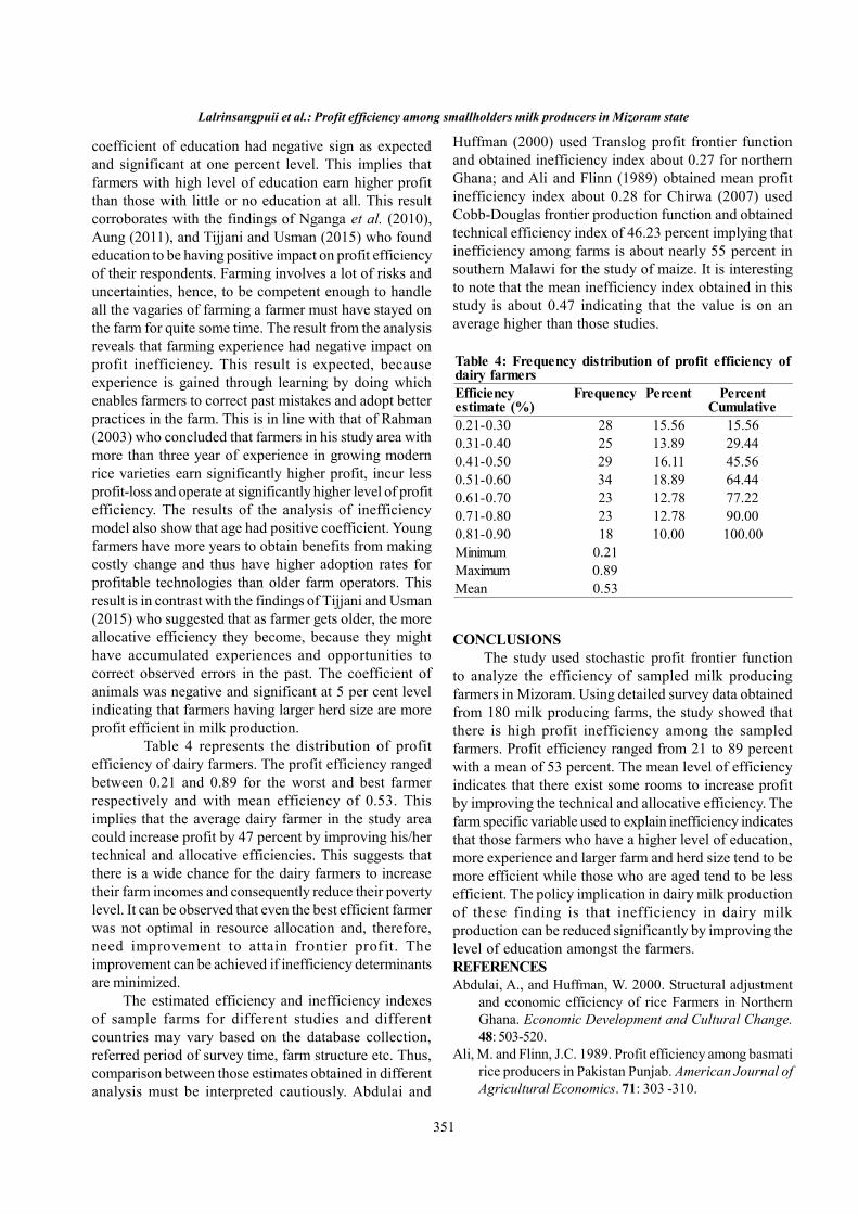
351
coefficient of education had negative sign as expectedand significant at one percent level. This implies thatfarmers with high level of education earn higher profitthan those with little or no education at all. This resultcorroborates with the findings of Nganga et al. (2010),Aung (2011), and Tijjani and Usman (2015) who foundeducation to be having positive impact on profit efficiencyof their respondents. Farming involves a lot of risks anduncertainties, hence, to be competent enough to handleall the vagaries of farming a farmer must have stayed onthe farm for quite some time. The result from the analysisreveals that farming experience had negative impact onprofit inefficiency. This result is expected, becauseexperience is gained through learning by doing whichenables farmers to correct past mistakes and adopt betterpractices in the farm. This is in line with that of Rahman(2003) who concluded that farmers in his study area withmore than three year of experience in growing modernrice varieties earn significantly higher profit, incur lessprofit-loss and operate at significantly higher level of profitefficiency. The results of the analysis of inefficiencymodel also show that age had positive coefficient. Youngfarmers have more years to obtain benefits from makingcostly change and thus have higher adoption rates forprofitable technologies than older farm operators. Thisresult is in contrast with the findings of Tijjani and Usman(2015) who suggested that as farmer gets older, the moreallocative efficiency they become, because they mighthave accumulated experiences and opportunities tocorrect observed errors in the past. The coefficient ofanimals was negative and significant at 5 per cent levelindicating that farmers having larger herd size are moreprofit efficient in milk production.
Table 4 represents the distribution of profitefficiency of dairy farmers. The profit efficiency rangedbetween 0.21 and 0.89 for the worst and best farmerrespectively and with mean efficiency of 0.53. Thisimplies that the average dairy farmer in the study areacould increase profit by 47 percent by improving his/hertechnical and allocative efficiencies. This suggests thatthere is a wide chance for the dairy farmers to increasetheir farm incomes and consequently reduce their povertylevel. It can be observed that even the best efficient farmerwas not optimal in resource allocation and, therefore,need improvement to attain frontier profit. Theimprovement can be achieved if inefficiency determinantsare minimized.
The estimated efficiency and inefficiency indexesof sample farms for different studies and differentcountries may vary based on the database collection,referred period of survey time, farm structure etc. Thus,comparison between those estimates obtained in differentanalysis must be interpreted cautiously. Abdulai and
Huffman (2000) used Translog profit frontier functionand obtained inefficiency index about 0.27 for northernGhana; and Ali and Flinn (1989) obtained mean profitinefficiency index about 0.28 for Chirwa (2007) usedCobb-Douglas frontier production function and obtainedtechnical efficiency index of 46.23 percent implying thatinefficiency among farms is about nearly 55 percent insouthern Malawi for the study of maize. It is interestingto note that the mean inefficiency index obtained in thisstudy is about 0.47 indicating that the value is on anaverage higher than those studies.
Lalrinsangpuii et al.: Profit efficiency among smallholders milk producers in Mizoram state
Table 4: Frequency distribution of profit efficiency ofdairy farmersEfficiencyestimate (%)
Frequency Percent PercentCumulative
0.21-0.30 28 15.56 15.560.31-0.40 25 13.89 29.440.41-0.50 29 16.11 45.560.51-0.60 34 18.89 64.440.61-0.70 23 12.78 77.220.71-0.80 23 12.78 90.000.81-0.90 18 10.00 100.00Minimum 0.21Maximum 0.89Mean 0.53
CONCLUSIONSThe study used stochastic profit frontier function
to analyze the efficiency of sampled milk producingfarmers in Mizoram. Using detailed survey data obtainedfrom 180 milk producing farms, the study showed thatthere is high profit inefficiency among the sampledfarmers. Profit efficiency ranged from 21 to 89 percentwith a mean of 53 percent. The mean level of efficiencyindicates that there exist some rooms to increase profitby improving the technical and allocative efficiency. Thefarm specific variable used to explain inefficiency indicatesthat those farmers who have a higher level of education,more experience and larger farm and herd size tend to bemore efficient while those who are aged tend to be lessefficient. The policy implication in dairy milk productionof these finding is that inefficiency in dairy milkproduction can be reduced significantly by improving thelevel of education amongst the farmers.REFERENCESAbdulai, A., and Huffman, W. 2000. Structural adjustment
and economic efficiency of rice Farmers in NorthernGhana. Economic Development and Cultural Change.48: 503-520.
Ali, M. and Flinn, J.C. 1989. Profit efficiency among basmatirice producers in Pakistan Punjab. American Journal ofAgricultural Economics. 71: 303 -310.

352
Indian J Econ Dev 12 (2): 2016 (April-June)
Anonymous. 2013. Agriculture statistical abstract 2012-13.Directorate of Agriculture (Crop Husbandry).Government of Mizoram, Aizawl - 796001.
Anonymous. 2014. Report on integrated sample survey forthe estimation of annual production of milk, eggs andmeat for the year 2013-2014. Directorate of AnimalHusbandry and Veterinary. Government of Mizoram,Aizawl -796001.
Anonymous. 2014a. Basic animal husbandry and fisheriesstatistics. Ministry of Agriculture, Department of AnimalHusbandry, Dairying and Fisheries, Krishi Bhawan, NewDelhi.
Aung, N. M. 2011. Agricultural efficiency of rice farmers inMyanmar: A case study in selected areas. IDEDiscussion Paper No. 306. Institute DevelopingEconomies, Jetro, Japan.
Battese, G. and Coelli, T. 1995. A model for technicalinefficiency effects in a stochastic frontier productionfunction for panel data. Empirical Economics. 20: 325-332.
Chirwa, E.W. 2007. Sources of technical efficiency amongsmallholder maize farmers in Southern Malawi. AERC
AcknowledgementThe authors acknowledge Director, ICAR-National Dairy Research Institute, Karnal-132001 (Haryana), India forproviding financial assistance and infrastructure to carry out the research work. The first author also acknowledgesthe University Grants Commission for providing financial assistant during the entire period of the research work.
Research Paper. African Economic Research Consortium,Nairobi.
Coelli, T.J. 1996. A guide to FRONTIER Version 4.1: Acomputer program for Stochastic Frontier Productionand Cost Function Estimation. CEPA. University of NewEngland, Armidale, NSW, 2351, Australia.
Kumar, A., Staal, S., Elumalai, K., and Singh, D.K. 2007.Livestock sector in North-Eastern Region of India: Anappraisal of performance. Agricultural EconomicsResearch Review. 20 (1): 255-272.
Kumbhakar, S.C. and Bhattacharyyas, A. 1992. Pricedistribution and resource-use inefficiency in Indianagriculture: A restricted profit function approach. Reviewof Economic and statistics. 74: 231-39.
Nganga, S.K., Kungu, J., N. de Ridder, and Herrero, M. 2010.Profit efficiency among Kenyan smallholders milkproducers: A case study of Meru-South district, Kenya.African Journal of Agricultural Research. 5 (4): 332-337.
Rahman, S. 2002. Profit efficiency among Bangladeshi ricefarmers. School of Economic Studies. The University ofManchester Oxford Road Manchester, M13 9PL England.

353
www.soed.in
Economic Analysis of Milk Production and Marketed Surplus inChittorgarh District of RajasthanR.L. Bairwa, A.K. Chauhan*, Bulbul G.. Nagrale, and Denny Franco
Department of Economics, Statistics and Management ICAR- NDRI, Karnal(Haryana)
*Corresponding author’s email: [email protected]
Received: April 24, 2015 Accepted: May 05 , 2016
Indian Journal of Economics and DevelopmentVolume 12 No. 2: 353-358
April-June, 2016DOI: 10.5958/2322-0430.2016.00147.5
ABSTRACTThe present study was conducted by selecting 150 milk producers adopting multistage stratified random samplingtechnique. The households were further post stratified into three herd size categories as small,medium and large usingcumulative square root frequency method. The distribution of sample household across each of the herd size categorieswere 68, 50 and 32, respectively. The study revealed that per day net maintenance cost was found higher for crossbredcow followed by buffalo and local cow. The high maintenance cost for crossbred cow was found, with higher cost ofconcentrate fed to these animals. In case of buffalo, the higher cost of maintenance was found with higher cost of greenfodder. The highest cost per litre was found, in case of local cow followed by buffalo and crossbred cow, which maypossible due to low milk productivity of these local cows. Cost of milk per litre was found decreased with increase in herdsize of milk producer across all type of animal breeds. Marketed surplus of milk was found more in the case of large herdsize category of households and there was no much difference in the case of medium and small herd size category ofhousehold. The higher amount of marketed surplus was disposed off to milk cooperatives society nearby sixty per cent oftotal surplus milk.
KeywordsCost of milk, marketed Surplus, milk productivity
JEL Codes
INTRODUCTIONLivestock sector provides employment to 70 million
farm families. Among these, 65 to 70 per cent are small,marginal farmers and landless labour. Further, dairy sectoris the major source of income and employment generationin the rural areas. Although, the share of agriculturalproducts/agriculture and allied sectors in Gross DomesticProduct (GDP) of the country has declined but the shareof livestock sector in the Ag. GDP is increasing. Duringthe past three decades, milk production in the countryhas increased from about 21.2 million tonnes in 1969 to137.6 million tonnes in 2013-14 (Anonymous, 2014).Dairy development is taking place in almost all the statesof the country.
Rajasthan is the second highest milk producing state(14.5 MT) after Uttar Pradesh (24.1 MT), among thetop ten milk producing states contributing 10.5 per centin India’s milk production (Anonymous, 2014).Thelivestock sector plays an important role in providing
supplementary income and employment to the majorityof resource poor farmers in the state. The large part ofthe state is arid or semi arid and fall under ‘Thar Desert’and adverse climatic conditions with scarcity of waterfor irrigation and erratic rainfall conditions. Therefore,livestock rearing plays an important role for livelihood inthe state.
Among the different districts of the state, Chittorgarhdistrict stands 3rd position in terms of number of cattleand buffalo population in the state. Total milk productionof district is about 222.95 thousand tonnes thus secured19th position in the state (Anonymous, 2012). The farmersrear dairy animals for alternative source of income andemployment for earning their livelihood. For launchingany dairy development programme in the area, the basicinformation on dairy farming practices and cost andreturns from milk production, marketed surplus and itsdisposal pattern is very useful to know for the planningpurpose. Keeping in mind the above facts, an attempt
D24, L11, Q12
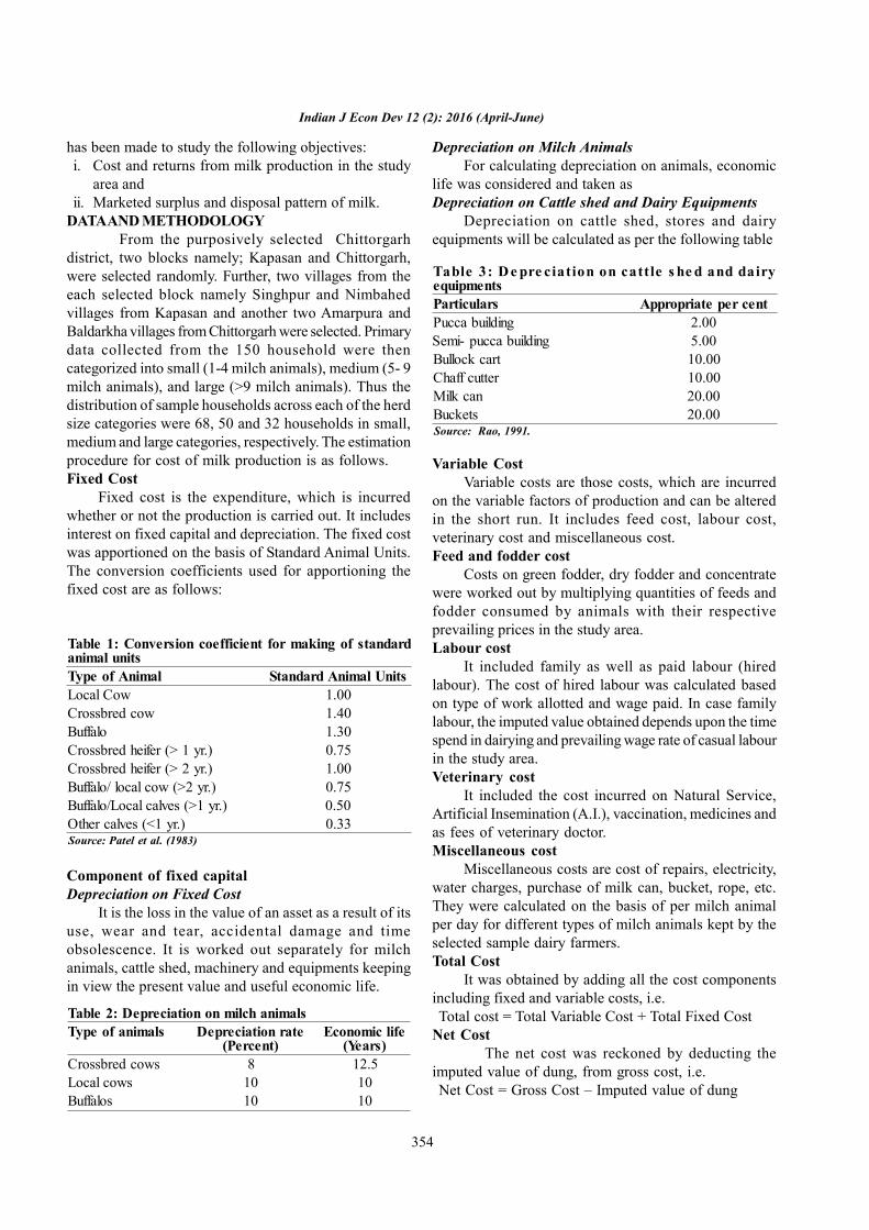
354
Indian J Econ Dev 12 (2): 2016 (April-June)
has been made to study the following objectives:i. Cost and returns from milk production in the study
area andii. Marketed surplus and disposal pattern of milk.
DATAAND METHODOLOGYFrom the purposively selected Chittorgarh
district, two blocks namely; Kapasan and Chittorgarh,were selected randomly. Further, two villages from theeach selected block namely Singhpur and Nimbahedvillages from Kapasan and another two Amarpura andBaldarkha villages from Chittorgarh were selected. Primarydata collected from the 150 household were thencategorized into small (1-4 milch animals), medium (5- 9milch animals), and large (>9 milch animals). Thus thedistribution of sample households across each of the herdsize categories were 68, 50 and 32 households in small,medium and large categories, respectively. The estimationprocedure for cost of milk production is as follows.Fixed Cost
Fixed cost is the expenditure, which is incurredwhether or not the production is carried out. It includesinterest on fixed capital and depreciation. The fixed costwas apportioned on the basis of Standard Animal Units.The conversion coefficients used for apportioning thefixed cost are as follows:
Variable CostVariable costs are those costs, which are incurred
on the variable factors of production and can be alteredin the short run. It includes feed cost, labour cost,veterinary cost and miscellaneous cost.Feed and fodder cost
Costs on green fodder, dry fodder and concentratewere worked out by multiplying quantities of feeds andfodder consumed by animals with their respectiveprevailing prices in the study area.Labour cost
It included family as well as paid labour (hiredlabour). The cost of hired labour was calculated basedon type of work allotted and wage paid. In case familylabour, the imputed value obtained depends upon the timespend in dairying and prevailing wage rate of casual labourin the study area.Veterinary cost
It included the cost incurred on Natural Service,Artificial Insemination (A.I.), vaccination, medicines andas fees of veterinary doctor.Miscellaneous cost
Miscellaneous costs are cost of repairs, electricity,water charges, purchase of milk can, bucket, rope, etc.They were calculated on the basis of per milch animalper day for different types of milch animals kept by theselected sample dairy farmers.Total Cost
It was obtained by adding all the cost componentsincluding fixed and variable costs, i.e.Total cost = Total Variable Cost + Total Fixed Cost
Net CostThe net cost was reckoned by deducting the
imputed value of dung, from gross cost, i.e.Net Cost = Gross Cost – Imputed value of dung
Table 1: Conversion coefficient for making of standardanimal unitsType of Animal Standard Animal UnitsLocal Cow 1.00Crossbred cow 1.40Buffalo 1.30Crossbred heifer (> 1 yr.) 0.75Crossbred heifer (> 2 yr.) 1.00Buffalo/ local cow (>2 yr.) 0.75Buffalo/Local calves (>1 yr.) 0.50Other calves (<1 yr.) 0.33Source: Patel et al. (1983)
Component of fixed capitalDepreciation on Fixed Cost
It is the loss in the value of an asset as a result of itsuse, wear and tear, accidental damage and timeobsolescence. It is worked out separately for milchanimals, cattle shed, machinery and equipments keepingin view the present value and useful economic life.
Table 2: Depreciation on milch animalsType of animals Depreciation rate
(Percent)Economic life
(Years)Crossbred cows 8 12.5Local cows 10 10Buffalos 10 10
Table 3: D e pre ciation on cattle s he d and dairyequipmentsParticulars Appropriate per centPucca building 2.00Semi- pucca building 5.00Bullock cart 10.00Chaff cutter 10.00Milk can 20.00Buckets 20.00Source: Rao, 1991.
Depreciation on Milch AnimalsFor calculating depreciation on animals, economic
life was considered and taken asDepreciation on Cattle shed and Dairy Equipments
Depreciation on cattle shed, stores and dairyequipments will be calculated as per the following table

355
Gross ReturnsGross returns were obtained by multiplying milk
yield of an individual animal with respective of prevailingprices in the study area:Gross Returns = Quantity of milk × Market price of milk
Price of MilkThe price of milk was calculated as average value
of all prices from different milk collection systems, itgiven on the basis of fat per cent in the milk. It is alsodepending upon type of milking animal and number oflactating period of animal.Net Returns
Net return was calculated by subtracting net costfrom gross returns:
Net Returns = Gross Returns – Net CostCost of Milk Production
In order to estimate the cost of per litre milk,the average net maintenance cost per animal per day wasdivided by average milk production per animal per day,that is,
per dayper animal producedTotal milkl per day per animacostNet
)itre (Cost per l `
Marketed Surplus of MilkMarketed surplus is that part of produce which is
actually brought to the market for sale. Overall marketedsurplus of milk was worked out according to herd sizecategory of sample households to the total marketedsurplus in each herd size category was also worked out.Disposal Pattern of Marketed Surplus of Milk
The disposal quantity consist of retention of liquidmilk and conversion of milk into different products atthe farm level and the remaining part out of total milkproduction that is available for sale liquid milk in themarket. The information regarding, quantity of milkconsumed at home, milk sold and the agency to whomsold i.e. co-operative societies, milk vendor or directly tothe consumers, tea stall/ hotel and others. The relativeshare of each marketing agency in the marketed surplusof milk was also worked out using tabular analysis.RESULTSAND DISCUSSION
The information regarding distribution of milchanimals across various categories of sample householdshas been presented in Table 4. The herd size across small,medium and large herd size category of households werefound to be 70, 138 and 133 of local cow 15, 24 and 27of crossbred cow 114, 189 and 216 of buffalo,respectively.
The overall average daily milk yield per milch animalswas found to be 1.94 litres for local cow, 4.86 litres forcrossbred cows, while it was 3.63 litres per day per milchanimal for buffalo (Table 5).
Average Quantity of Feed and Fodder of MilchAnimals
The information regarding average quantity of feedand fodder of milch animals has been presented in Table6. The information in the table revealed that the averagequantity of feed and fodder for local cow was found17.69 kg green fodder, 6.36 kg dry fodder, 0.75 kgconcentrate, and 0.01 kg Minerals. It was found 29.00kg green fodders, 6.72 dry fodders, 3.47 kg concentrate,and 0.05 kg mineral mixture for crossbred cow, while Itwas found 31.33 kg green fodders, 9.71 kg dry fodders,2.22 kg concentrate, and 0.04 kg mineral mixture forbuffalo.
Table 5: Average milk production of different milchanimalsType of milch animals Milk production (Litre/ day)Local cow 1.94Crossbred cow 4.86Buffalo 3.63
Maintenance Cost and Returns of Local Milch CowIt may be seen from Table 7 that the overall average
daily net maintenance cost per milch local cow wasworked out as `74.67, category-wise net maintenancecost was worked out as `75.63, `75.19 and `73.18 forsmall, medium and large herd size category of samplehouseholds, respectively. The overall net return per milchlocal cow was negative as `-9.79, while it was alsonegative as `-11.83, `-10.31 and `-7.21 across small,medium and large herd size category of households,respectively. The local cow gives negative surplus dueto its less productivity. Overall variable cost accountedfor 85.01 per cent of the gross cost where feed was themajor cost component with the total share of 65.42 percent.
The overall labour cost accounted for 14.76 per cent
Table 6: Average quantity of feed and fodder of milchanimals
(Kg/animal/day)Particular Green
fodderDry
FodderConcentrate Mineral
MixtureLocal cow 17.69 6.36 0.75 0.01Crossbred 29.00 6.72 3.47 0.05Buffalo 31.33 9.71 2.22 0.04
Bairwa et al.: Economic analysis of milk production and marketed surplus in Chittorgarh
Table 4: Distribution of milch animals across differentherd size categoriesHerd size Local cow Cross bred cow BuffaloSmall (1-4) 70 15 114Medium (5-9) 138 24 189Large (>9) 133 27 216Overall 341 66 519

356
Indian J Econ Dev 12 (2): 2016 (April-June)
Maintenance Cost and Returns of Milch CrossbredCow
It may be seen from Table 8 that the overall averagedaily net maintenance cost per milch crossbred cow wasworked out as `133.05, category-wise net maintenancecost was worked out as `145.35, `128.90 and `124.94for small, medium and large herd size category ofhouseholds, respectively. The overall net return per milchcrossbred cow was `25.73 while these were workedout `9.53, `28.29 and `39.34 for small, medium andlarge herd size category of households, respectively.Overall variable cost accounted for 78.60 per cent of thegross cost where feed was the major cost componentwith the total share of 54.38 per cent. The overall labourcost accounted for 10.67 per cent of the gross cost whileit was found 9.02, 11.23 and 12.01 per cent for small,medium and large herd size category of households,respectively. The overall average cost per liter was found`26.71 while these average costs were found `29.99,`26.12 and `24.19 for small, medium and large herd sizecategory of households, respectively.
Overall fixed cost is accounted for 21.40 percentof the gross cost, while it was found 21.91, 20.50 and
of the gross cost while it was found 16.47, 13.99 and13.80 per cent for small, medium and large herd sizecategory of sample households, respectively. The overallaverage cost per litre of milk was observed `37.05 whilecategory-wise these costs were found `38.23, `37.31and `35.64 for small, medium and large herd size categoryof households, respectively. The overall fixed costaccounted for 14.99 per cent of the gross cost whilethese costs were found 14.86, 14.66 and 15.47 per centacross small, medium and large herd size category ofhouseholds, respectively. Overall loss from local milchcow per litre was `-5.05 while the highest loss was found`-6.23, for small category and the lowest loss was found`-3.64 for large category. Negative returns from localcows were attributed to the low milk yield of this species.The overall average milk yield per milch animal wasobserved 1.94 litre, while it was found 1.90, 1.94 and1.98 litres for small, medium and large herd size categoryof households, respectively. The relatively higher perlitre cost of milk production was observed in the presentstudy could be mainly attributed to the high cost of greenfodder as less milk yield which accounted for 29.18 percent of gross cost.
Table 7: Maintenance cost and returns per local milchcow
(`/animal/day)Cost component Herd size category
Small Medium Large OverallFeed and Fodder 48.02
(63.49)49.77
(66.19)48.75
(66.61)48.85
(65.42)Labour 12.45
(16.47)10.52
(13.99)10.1
(13.80)11.02
(14.76)Miscellaneous 3.92
(5.18)3.88
(5.16)3.01
(4.12)3.6
(4.83)Total variable cost(A)
64.39(85.14)
64.17(85.34)
61.86(84.53)
63.47(85.01)
Depreciation on fixedcost
9.44(12.48)
9(11.97)
9.54(13.04)
9.33(12.49)
Interest on fixed cost 1.8(2.38)
2.02(2.69)
1.78(2.43)
1.87(2.50)
Total fixed cost (B) 11.24(14.86)
11.02(14.66)
11.32(15.47)
11.2(14.99)
Gross cost (A+B) 75.63(100.0-
0)
75.19(100.00)
73.18(100.00)
74.67(100.00)
Value of dung 3 2.8 2.61 2.8Net cost 72.63 72.39 70.57 71.87Sale price of milk `per litre
32 32 32 32
Milk production inlitres
1.9 1.94 1.98 1.94
Gross returns 60.8 62.08 63.36 62.08Net returns -11.83 -10.31 -7.21 -9.79Cost per litre 38.23 37.31 35.64 37.05Net returns per litres -6.23 -5.31 -3.64 -5.05Figures in parentheses indicate percentage to gross cost
Table 8: Maintenance cos t and re turns per milchcrossbred cow
(`/animal/day)Cost component Herd Size Category
Small Medium Large OverallCost of feed andfodder
73.94(50.88)
72.3(56.09)
70.84(56.70)
72.35(54.38)
Labour 13.12(9.02)
14.47(11.23)
15.01(12.01)
14.2(10.67)
Miscellaneous 26.44(18.19)
15.71(12.18)
11.93(9.55)
18.03(13.55)
Total variable cost(A)
113.5(78.09)
102.48(79.50)
97.78(78.26)
104.58(78.60)
Depreciation onfixed capital
21.88(15.05)
20.82(16.15)
21.37(17.10)
21.35(16.05)
Interest on fixedcapital
9.97(6.86)
5.6(4.35)
5.79(4.64)
7.12(5.35)
Total fixed cost (B ) 31.85(21.91)
26.42(20.50)
27.16(21.74)
28.47(21.40)
Gross cost (A+B) 145.35(100.00)
128.9(100.00)
124.94(100.00)
133.05(100.00)
Value of dung 3.52 3.27 3 3.26Net cost 141.83 125.63 121.94 129.79Sale price of milk`/litre
32 32 32 32
Milk production inlitre
4.73 4.81 5.04 4.86
Gross returns 151.36 153.92 161.28 155.52Net returns 9.53 28.29 39.34 25.73Cost per litre 29.99 26.12 24.19 26.71Net returns per litre 2.01 5.88 7.81 5.29Figures in parentheses indicate percentage to gross cost

357
of households, respectively. Overall variable costaccounted for 84.89 per cent of the gross cost wherefeed was the major cost component with the total shareof 65.58 per cent. The overall labour cost accounted for14.39 per cent of the gross cost while category-wisethese labour costs were found 14.51, 14.64 and 13.99per cent for small, medium and large herd size categoryof households, respectively. The overall average cost perliter was found `28.58 while it was found `32.23, `29.56and `24.81 for small, medium and large herd size categoryof households, respectively. The overall fixed costaccounted for 15.11 per cent of the gross cost while itwas found 14.36, 14.45 and 16.63 percent for small,medium and large herd size category of households,respectively.
This was to be found in agreement with the findingsof Chandra (1998). The overall average milk yield permilch animal was observed 3.63 litres while it was 3.34,3.49, and 4.05 litres for small, medium and large herdsize categories of households, respectively. The overallaverage returns per litre was found `7.42 while it wasfound 3.77, `6.44 and `11.19 for small, medium andlarge herd size category of households, respectively. Therelatively higher per litre cost of milk production observedin the present study could be mainly attributed to thehigh cost of green fodder which accounted for 27.88per cent of gross cost. The overall sale price per litre ofmilk was found to be `36.00.Average Milk Production, Consumption andMarketed Surplus
The information regarding average milk production,consumption and marketed surplus of differenthousehold’s category has been presented in Table 10.The average milk production was found 8.6, 20.84 and39.79 litres per day for small, medium and large herdsize category of households, respectively in the studyarea. The average milk consumption was found 1.76,3.45 and 4 .11 litres for small, medium and large categoriesof households, respectively. Average milk marketedsurplus was found 79.48, 83.45 and 89.67 percent oftotal milk production for small, medium and large herd
21.74 percent for small, medium and large herd sizecategory of households, respectively. This was to befound in agreement with the findings of Chandra (1998).The overall average milk yield per milch animal wasobserved 4.86 litres while it was found 4.73, 4.81 and5.04 litres for small, medium and large herd size categoriesof households, respectively.The overall average returnsper litre was found `5.29 while it was found `2.01, `5.88and `7.81 for small, medium and large herd size categoryhouseholds, respectively. The relatively higher per litrecost of milk production observed in the present studycould be mainly attributed to the high cost of concentratewhich accounted for 24.88 percent of gross cost .Theoverall sale price per litre of milk was found to be `32.00.Maintenance Cost and Returns of Milch Buffalo
It may be seen from Table 9 that the overall averagedaily net maintenance cost per milch buffalo was workedout as `107.18; category-wise these costs were found`111.48, `106.42 and `103.64 for small, medium andlarge herd size category of sample households,respectively. The overall net return per milch buffalo wasworked out `26.92 while it was found `12.59, `22.49and `45.31 for small, medium and large herd size category
Table 9: Maintenance cost and returns per milch buffalo(`/animal/day)
Cost component Herd size categorySmall Medium Large Overall
Cost of feed andfodder
71.55(64.18)
70.55(66.29)
68.76(66.34)
70.29(65.58)
Labour 16.18(14.51)
15.58(14.64)
14.5(13.99)
15.42(14.39)
Miscellaneous 7.75(6.95)
4.92(4.62)
3.15(3.04)
5.27(4.92)
Total variable cost (A) 95.48(85.64)
91.05(85.55)
86.41(83.37)
90.98(84.89)
Depreciation on fixedcapital
13.53(12.14)
13.41(12.60)
15.45(14.91)
14.13(13.18)
Interest on fixedcapital
2.47(2.22)
1.96(1.85)
1.78(1.72)
2.07(1.93)
Total fixed cost (B ) 16(14.36)
15.37(14.45)
17.23(16.63)
16.2(15.11)
Gross cost (A+B) 111.48(100.00)
106.42(100.00)
103.64(100.00)
107.18(100.0-
0)Value of dung 3.83 3.27 3.15 3.42Net cost 107.65 103.15 100.49 103.76Sale price of milkRs/litre
36 36 36 36
Milk production inlitres
3.34 3.49 4.05 3.63
Gross returns 120.24 125.64 145.8 130.68Net returns 12.59 22.49 45.31 26.92Cost per liters 32.23 29.56 24.81 28.58Net returns per litre 3.77 6.44 11.19 7.42Figures in parentheses indicate percentage to gross cost
Table 10: Average milk production, consumption andmarketed surplus of among different categories ofhouseholdsCategory (Litres/day) Milk marketed
surplus as percentageof milk production
Milkproduction
Milkconsumption
Small (1-4) 8.6 1.76 6.83(79.48)
Medium (5-9) 20.84 3.45 17.39(83.45)
Large ( >9) 39.79 4.11 35.68(89.67)
Figures in parentheses indicate percentage of the milk production
Bairwa et al.: Economic analysis of milk production and marketed surplus in Chittorgarh district of Rajasthan

358
Indian J Econ Dev 12 (2): 2016 (April-June)
size category of households, respectively. Inter-categoryanalysis revealed that the marketed surplus increased withthe increase in size of herd size category.Disposal Pattern of Milk
Milk producers of small category disposed off thesurplus quantity of milk to dairy co-operative (60.87percent), halwai and hotel (23.51 percent), milk vendor(10.68 percent), private dairy (3.22 percent) and localconsumer (1.72 percent). Milk producers of mediumcategory disposed off the surplus quantity of milk to dairyco-operative (70.57 percent), halwai and hotel (18.58percent), milk vendor (6.01 percent), private dairy (3.32percent) and local consumer (1.52 percent). Milkproducers of large category disposed off the surplusquantity of milk to dairy co-operative (65.05 percent),halwai and hotel (17.61 percent), local consumer (7.74percent), milk vendor (5.90 percent), private dairy (3.70percent).
increase the share of cooperatives will boost the dairydevelopment activities and economy of the milk producersin the study area.REFERENCESAnonymous. 2012. Report on animal husbandry, dairying
and fisheries. Government of India. New Delhi.Anonymous. 2014. Basic animal husbandry and fisheries
report. Government of India, Ministry of Agriculture andFarmers Welfare, Department of Animal Husbandry,Dairying and Fisheries, Krishi Bhawan, New Delhi.
Desai, V. 2005. An economic analysis of Milk productionand disposal pattern of milk in rural area of Bidardistrict (Karnataka). M.Sc. Thesis submitted to NDRI(Deemed University), Karnal, Haryana.
Ghule, A.K. 2010. Economics of milk production and itsdisposal pattern on commercial dairy farms inAhmednagar district of Maharashtra. M.V.Sc. Thesissubmitted to NDRI (Deemed University), Karnal,Haryana, India.
Khan, A.R. 2006. Economic analysis of milk productionsystem in New Alluvial Zone of West Bengal, Ph.D.Thesis submitted to NDRI (Deemed University), Karnal,Haryana, India.
Khoveio, M. 2011. Economics of milk production, marketedsurplus and its disposal pattern in Nagaland. M.V.Sc.Thesis submitted to NDRI (Deemed University), Karnal,Haryana, India..
Nagrale, B.G. 2011. Economics of milk production in Vidarbharegion of Maharashtra. M.V.Sc. Thesis submitted toNDRI (Deemed University), Karnal, Haryana, India.
Prasad, S.M. 2010. Economic analysis of dairy productionsystem in Nanded district of Maharashtra. M.V.Sc.Thesis submitted to NDRI (Deemed University), Karnal,Haryana, India.
Rajendran, K. and Prabaharan, R. 1993. A study on production,consumption and disposal of milk in Dharampuri districtof Tamil Nadu. Indian Journal of Dairy Sciences. 46(19): 458-459.
Shah, D., Jain, D.K., and Sharma, K.N.S. 1995. Milk productionof Bulandshahar disrict of Uttar Pradesh. IndianJournal of Dairy Sciences. 48 (8): 505-506.
Sharma, V.P. and Sigh, R.V. 1994. An economic analysis ofmilk production by different breeds of milch animals inhumid-temperate zone of Himachal Pradesh. IndianJournal of Dairy Sciences. 47 (9): 749-755.
Shiyani, R.L. and Singh, R.V. 1995. Economics of milkproduction- A comparative study. Indian Journal ofDairy Sciences. 48 (1): 21-26.
Milk producers of all categories disposed off thesurplus quantity of milk to dairy co-operative (66.28percent), halwai and hotel (18.78 percent), local consumer(4.82 percent), milk vendor (6.62 percent), private dairy(3.50 percent).CONCLUSIONS
The cost and returns measures of milk productionobtained in present study suggested that buffalo milkproduction is relatively more profitable than cow in thestudy area on the basis of net returns per litre of milk.Thus sound economic logic exists for persuading buffalowhile negative condition was found for local cow.Therefore, efforts should be made to upgrade local cowthrough efficient livestock support services so that itsnet returns can be increased. The study showed thatMPCS collects more than 60 per cent of marketed surplusof milk in the study area and these were found morefavorable to the milk producers, therefore, efforts to
Table 11: Disposal pattern of milk in percentageParticular Small Medium Large overallDirectly to local consumer 1.72 1.52 7.74 4.82Selling to milk vendor 10.68 6.01 5.90 6.62Selling to Halwai and hotel 23.51 18.58 17.61 18.78Selling to dairy co-operative 60.87 70.57 65.05 66.28Selling to private dairy 3.22 3.32 3.70 3.50

359
www.soed.in
Economics and Growth Performance of ChrysanthemumFlower in Tumkur district of KarnatakaGunabhagya1*, S.S. Guledgudda2 and B.C. Rajur2
1Department of Agricultural Economics, College of Agriculture [UAS-R], Raichur - 584102, Karnataka (E-mail: ).2College of Agriculture [UAS-D], Bijapur-586101, Karnataka
*Corresponding author’s email: [email protected]
Received: February 03, 2016 Accepted: April 15, 2016
Indian Journal of Economics and DevelopmentVolume 12 No. 2: 359-364
April-June, 2016DOI: 10.5958/2322-0430.2016.00148.7
ABSTRACTTumkur district is well known for flower production. It is the major flower-growing district in Karnataka. Tumkur districtstands first in area and production of chrysanthemum flower cultivation. Hence, Tumkur district has been selected for thestudy purposively. The area under chrysanthemum is increasing at a higher rate (14.36 per cent per annum) in Tumkur butin case of Karnataka as a whole the growth in area was 5.86 percent per annum while productivity of chrysanthemumflower (-2.40 percent) in Tumkur district found to be negatively growing. Further it could be observed from the study that,per hectare cost of cultivation of chrysanthemum flower was `61767. And the average annual gross return realized perha, by the respondents amounted to `190541. Thus, it could be summarised that cultivation of chrysanthemum flowerprovided assured return of `128773 per ha even after recovering the fixed costs and variable costs.
KeywordsEconomics, Growth performance, cost and returns of chrysanthemum, Netreturns
JEL CodesB42, C18, C20, Q18
INTRODUCTIONFloriculture is an important agribusiness, gaining
commercial importance in Indian agriculture. India beinga tropical country has several advantages in floricultureproduction, mainly consists of cut flowers and ornamentalfoliage plants. The flowers, which are more important incut flower trade, are orchid, rose, carnation,chrysanthemum and gladiolus. Most of these flowers aregrown under protected conditions. About 2.15 lakhhectare of area was under floriculture cultivation in 2014-15 (Anonymous, 2012).
As chrysanthemum flower (Chrysanthemummorifolium) is popularly called the queen of the east itadmires and enthusiasts all over the world. It belongs tothe family Asteraceae and recognized as a potent flowercrop in many countries and widely grown in open fieldsin India for loose flowers. It is a native of china and wasunder cultivation even before 500 BC in that country. Itis often described as the autumn queen as it blooms inNovember-December. Chrysanthemum is the Nationalflower of Japan, and it occupies third rank in the
international cut flower trade next to carnation and rose.The year 1995-96 was celebrated as an International yearof chrysanthemum.
The country has exported 4.10 million tons offloriculture products worth `374.32 crores in 2013-14and the major export destinations were USA, Germany,Netherlands, United Kingdom, Japan, Canada and UAEduring the same period.
The major flower growing states in India areKarnataka, Tamil Nadu and Andhra Pradesh in the South,West Bengal in the East, Maharashtra in the West andRajasthan, Delhi and Haryana in the North. Presently anarea of about 60,000 hectare is under floriculture incountry and estimated production is 2,00,000 tonnes ofloose flowers and 500 million cut flowers (Anonymous,2012a).
Among the flower crops grown in Karnatakachrysanthemum ranks third in terms of area (3,157 lakhha) and second in terms of production (23,493 tonnes)followed by jasmine which ranks second in terms of area(4097 lakh ha) and third in terms of production (21,299

360
Indian J Econ Dev 12 (2): 2016 (April-June)
Table 1: Trends in Area, production and productivity ofchrysanthemum flower in Karnataka and Tumkur , 2001-02 to 2011-12Particulars Growth rates (Percent per annum)
Tumkur KarnatakaArea 14.63* 5.86*
Production 11.61* 7.03*
Productivity -2.40** 1.11Area 50.05 22.24Production 53.6 24.15Productivity 13.93 11.53* and ** Significant at 1 and 5 percent level
tonnes) (Anonymous, 2012b).In southern part of the country, chrysanthemum
flower is mostly grown in farmer fields for supply to themarkets as loose flowers for garlands, hair decorationby the ladies and for religious ceremonies. Yellow colouredflowers are preferred in south, while in North varioushues of red, purple, yellow and white flowers are grownin abundance.
Tumkur district is well known for flower production.It is the major flower-growing district in Karnataka.Tumkur district stands first in area and production ofchrysanthemum flower cultivation. Hence, Tumkurdistrict has been selected for the study purposively (Area,Production and Productivity of Chrysanthemum flowerin Karnataka (2012-13) is given in Appendices-I).
In Tumkur district, fresh flowers are being cultivatedin an area of 2,878 hectares (2012) of whichchrysanthemum flower occupied first place (1162 ha)followed by Jasmine-Multiflora (730 ha) and Aster (593ha) (Anonymous, 2012a). Thus, a chrysanthemum flowerforms an important flower crop of the district andpromotes livelihood to the larger sector of the farmingcommunity. The area under this crop is increasing yearby year in the district. This flower crop is very oftensubjected to wide price fluctuations in the domesticmarkets. There is no systematic organising flower marketlike other fruits and vegetables markets.
Chrysanthemum is high value and labour intensivecrop and it is cultivated by most of the farmers on smallscale. The knowledge on cost of cultivation and returnsand growth performance of area, production andproductivity of chrysanthemum flower cultivation is veryessential for the cultivators to adjust and coordinate theavailable resources in a profitable manner. In the backdrop of this the present study was carried out with thefollowing objectives:i. to analyse the growth in chrysanthemum flower
production in Tumkur district andii. to workout the cost and returns in chrysanthemum
flower production;MATERIALAND METHODS
The study was conducted during 2013-14 and itincludes both primary and secondary data. Necessarysecondary time series data on area, production andproductivity was collected from Directorate ofHorticulture, Bangalore, District Horticulture Office,Tumkur and office of the Senior Assistant Director ofHorticulture, Tumkur, Sira and Koratagere taluks. Thesecondary data collected for the study included district-wise area under chrysanthemum flower in Karnataka,taluk-wise area under chrysanthemum flower in Tumkurdistrict, cropping pattern, etc. And for evaluating the
specific objectives of the study, important primary datarelating to production of chrysanthemum flower werecollected from the selected 60 sample farmers in the studyarea. The data collected from the respondents includessome general information, cost of cultivation and inputuse, etc.
The compound growth rate analysis was carriedout to ascertain the growth in area, production andproductivity and to work out the cost of cultivation farmmanagement cost concepts and descriptive statistics wereused.Compound Annual Growth Rate Analysis: Forevaluating the trend in area and production ofchrysanthemum flower in Tumkur district and selectedtaluks, an exponential form of the growth function wasused.Instability Analysis: The extent of variability in area,production and productivity of chrysanthemum flowerwas analysed through Coefficient of Variation.Farm Management Cost Conceptsa) Cost A1/ Cost A2: Sum of planting material, weeding,application of manure and fertilizers, value of plantprotection chemicals, irrigation charges, value of hiredlabour, harvesting, imputed value of family labour, intereston working capital, land revenue and depreciation.b) Cost B1: Cost A1 + Interest on fixed capitalc) Cost B2: Cost B1 + Rental value of landd) Cost C1: Cost B1 + Imputed value of family laboure) Cost C2: Cost B2 + Imputed value of family labourf) Farm business income = Gross income-Cost A1g) Family labour income = Gross income-Cost B2
RESULTSAND DISCUSSIONTable 1 presents the growth rate of area, production
and productivity of chrysanthemum flower in Tumkurdistrict and Karnataka state as whole since 2001-02through 2011-2012. The area and production of Tumkurdistrict has registered a positive and significant growthrate of 14.63 and 11.61 percent per annum respectivelywhile their productivity registered negative growth rateof 2.4 percent per annum during the same period. This
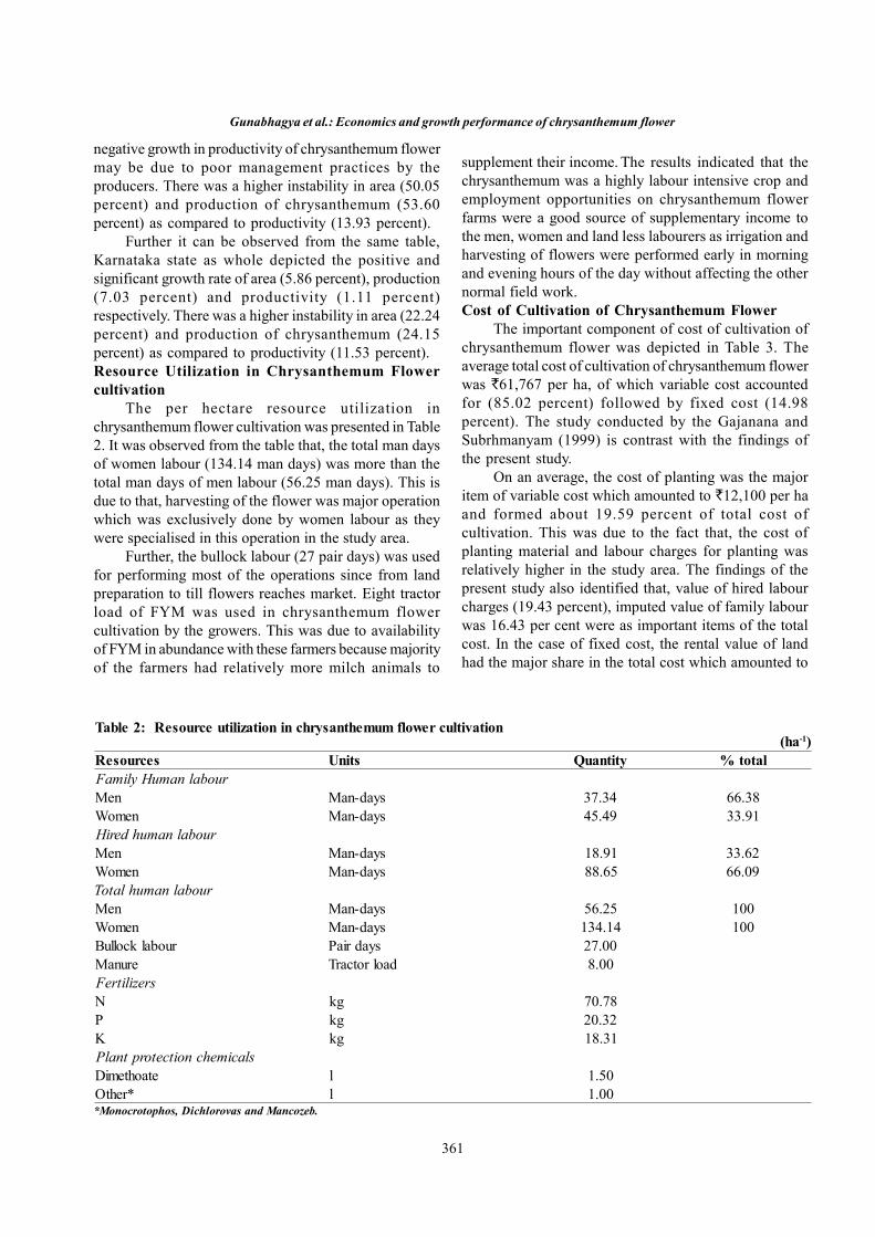
361
Gunabhagya et al.: Economics and growth performance of chrysanthemum flower
negative growth in productivity of chrysanthemum flowermay be due to poor management practices by theproducers. There was a higher instability in area (50.05percent) and production of chrysanthemum (53.60percent) as compared to productivity (13.93 percent).
Further it can be observed from the same table,Karnataka state as whole depicted the positive andsignificant growth rate of area (5.86 percent), production(7.03 percent) and productivity (1.11 percent)respectively. There was a higher instability in area (22.24percent) and production of chrysanthemum (24.15percent) as compared to productivity (11.53 percent).Resource Utilization in Chrysanthemum Flowercultivation
The per hectare resource utilization inchrysanthemum flower cultivation was presented in Table2. It was observed from the table that, the total man daysof women labour (134.14 man days) was more than thetotal man days of men labour (56.25 man days). This isdue to that, harvesting of the flower was major operationwhich was exclusively done by women labour as theywere specialised in this operation in the study area.
Further, the bullock labour (27 pair days) was usedfor performing most of the operations since from landpreparation to till flowers reaches market. Eight tractorload of FYM was used in chrysanthemum flowercultivation by the growers. This was due to availabilityof FYM in abundance with these farmers because majorityof the farmers had relatively more milch animals to
Table 2: Resource utilization in chrysanthemum flower cultivation(ha-1)
Resources Units Quantity % totalFamily Human labourMen Man-days 37.34 66.38Women Man-days 45.49 33.91Hired human labourMen Man-days 18.91 33.62Women Man-days 88.65 66.09Total human labourMen Man-days 56.25 100Women Man-days 134.14 100Bullock labour Pair days 27.00Manure Tractor load 8.00FertilizersN kg 70.78P kg 20.32K kg 18.31Plant protection chemicalsDimethoate l 1.50Other* l 1.00*Monocrotophos, Dichlorovas and Mancozeb.
supplement their income. The results indicated that thechrysanthemum was a highly labour intensive crop andemployment opportunities on chrysanthemum flowerfarms were a good source of supplementary income tothe men, women and land less labourers as irrigation andharvesting of flowers were performed early in morningand evening hours of the day without affecting the othernormal field work.Cost of Cultivation of Chrysanthemum Flower
The important component of cost of cultivation ofchrysanthemum flower was depicted in Table 3. Theaverage total cost of cultivation of chrysanthemum flowerwas `61,767 per ha, of which variable cost accountedfor (85.02 percent) followed by fixed cost (14.98percent). The study conducted by the Gajanana andSubrhmanyam (1999) is contrast with the findings ofthe present study.
On an average, the cost of planting was the majoritem of variable cost which amounted to `12,100 per haand formed about 19.59 percent of total cost ofcultivation. This was due to the fact that, the cost ofplanting material and labour charges for planting wasrelatively higher in the study area. The findings of thepresent study also identified that, value of hired labourcharges (19.43 percent), imputed value of family labourwas 16.43 per cent were as important items of the totalcost. In the case of fixed cost, the rental value of landhad the major share in the total cost which amounted to

362
Indian J Econ Dev 12 (2): 2016 (April-June)
`6,650 per ha (10.77 percent). This was mainly due tothe higher rental value of land as they were located veryclose to city.Cost and Returns Structure for ChrysanthemumFlower
The average quantity of flowers produced and grossreturns realized per ha have been discussed in this section.
The per hectare cost of cultivation of chrysanthemumflower was `61,767. And the average annual gross returnrealized per ha, by the respondents amounted to `1,90,541(Table 4). It was interesting to note that the gross incomewas high due to higher value of flowers especially duringwinter season as this is the season of marriages andfestivals and also there was less supply of flowers in themarket. The similar phenomena were observed in caseof total returns also. The study conducted by Swati
Table 4: Costs and returns structure of chrysanthemumflowerParticulars Amount (`/ ha)Operational cost 52512.00Overhead cost 9255.00Cost of cultivation 61767.00Cost A1 44022.00Cost A2 44022.0.00Cost B1 44967.00Cost B2 51617.00Cost C1 55117.00Cost C2 61767.00Yield (Kg/ha) 7622.00Gross Income 190541.00Farm Business income 146519.00Family Labour income 138923.00Net income 128773.00Return per rupee of investment 2.00Cost of Production (`/Kg) 8.00
Table 3: Cost of cultivation of chrysanthemum flowerParticulars Amount (`) Percent of total costVariable costPlanting 12,100 19.59Weeding 1,703 2.76Application of manures and fertilizers 3,600 5.83Value of plant protection chemicals 1,300 2.1Irrigation 2,100 3.4Value of laboura) Value of hired labour 12,002 19.43b) Imputed value of family labour 10,150 16.43Harvesting 5,668 9.18Interest on working capital @ 8% 3,890 6.3Sub-total 52,512 85.02Fixed costRental value of land 6,650 10.77Land revenue 510 0.83Depreciation on implements and machineries 1,150 1.86Interest on fixed capital @ 12% 945 1.53Sub-total 9,255 14.98Total cost 61,767 100
Table 3: Cost of cultivation of chrysanthemum flowerParticulars Amount
(`)Percent oftotal cost
Variable costPlanting 12,100 19.59Weeding 1,703 2.76Application of manures and fertilizers 3,600 5.83Value of plant protection chemicals 1,300 2.1Irrigation 2,100 3.4Value of laboura) Value of hired labour 12,002 19.43b) Imputed value of family labour 10,150 16.43Harvesting 5,668 9.18Interest on working capital @ 8% 3,890 6.3Sub-total 52,512 85.02Fixed costRental value of land 6,650 10.77Land revenue 510 0.83Depreciation on implements andmachineries
1,150 1.86
Interest on fixed capital @ 12% 945 1.53Sub-total 9,255 14.98Total cost 61,767 100

363
Gunabhagya et al.: Economics and growth performance of chrysanthemum flower
(2001) also revealed the similar pattern of behaviour ofreturns.
It was observed that the cost of producing one Kgof chrysanthemum flower was `8.00. And return fromrupee investment was `2.00. The finding of the presentstudy was much more than the study conducted by Patil(1985). This might be due to increase in cost due to highercharges of labour, electricity etc.,
Thus, it could be summarised that cultivation ofchrysanthemum flower provided assured return of`1,28,773 per ha even after recovering the fixed costsand variable costs. The findings of the present study werein line with Swati (2001) study on chrysanthemum inMaharashtra.CONCLUSIONS
Tumkur district is well known for flower productionand it stands first in area and production ofchrysanthemum flower cultivation (2011-12). The studyaims to analyze growth rate in area, production,productivity, utilization pattern and cost and returnsstructure. The growth rate analysis indicated that theincrease in production of chrysanthemum was due tothe increase in area, rather than productivity, which callsfor intensive efforts to increase the productivity ofchrysanthemum in the study area. Chrysanthemum flowercultivation has found to be little capital intensive and riskyto overcome such type of situations, chrysanthemum
cultivation needs to be insured. The resources like humanlabour, fertilizers, plant protection chemicals and irrigationcan be used optimally in order to get maximum returnsfrom the chrysanthemum cultivation. Proper marketingfacilities need to be developed in the study area, and further,there is a need to establish regulated market for floriculturecrops like of fruits and vegetables.REFERENCESAnonymous. 2012. Directorate of Horticulture, Lalbagh,
Bangalore.Anonymous. 2012a. Agriculture and Processed Food
Products Export Development Authority, Bangalore.Anonymous. 2012b. Office of the Assistant Director of
Horticulture, Tumkur, and District Statistical Office,District Department of Horticulture, Tumkur.
Gajanana, T. M. and Subrahmanyam, K.V. 1999. Economicsof production and marketing of Anthuriums in Karnataka.Agricultural Economics Research Review. 12 (1): 48-55.
Patil, S.T. 1985. Production and marketing of chrysanthemumin Dharwad district, Karnataka - An economic analysis.M.Sc. (Agri.) Thesis submitted to University ofAgricultural Sciences, Dharwad.
Swati, N.T. 2001. Economics of production and marketing ofchrysanthemum in Pune district. M.Sc. Thesis submittedto Mahatma Pule Krishi Vidyapeeth, Rahuri,Maharashtra.

364
Indian J Econ Dev 12 (2): 2016 (April-June)
Appendix-IArea, production and productivity of chrysanthemum in Tumkur (2001-02 to 2011-12)
Year Area (ha) Production (tonnes) Productivity (tonnes/ ha)2000-01 275 4125 41252001-02 273 3958.5 40952002-03 277 3878 41552003-04 291 3928.5 43652004-05 406 5278 60902005-06 539 6737.5 80852006-07 601 7212 90152007-08 792 9108 118802008-09 705 7755 105752009-10 904 9275.04 135602010-11 643 6430 96452011-12 1162 17430 17430Source: District Department of Horticulture, Tumkur (2012).
Appendix-IIArea, production and productivity of chrysanthemum flower in Karnataka
Year Area (ha) Production (tonnes) Productivity (tonnes/ ha)2000-01 2945 26033.00 35340.002001-02 3097 37674.00 37164.002002-03 3010 41741.00 42140.002003-04 2964 36419.00 36427.562004-05 3719 41843.00 40907.132005-06 3521 49266.00 49254.592006-07 4046 56474.00 56648.902008-09 4429 54092.00 54078.092009-10 4815 57929.00 57885.912010-11 4884 56674.00 56654.402011-12 5290 65180.00 65167.002012-13 4639 59826.00 59846.45Source: Statistical Wing, Directorate of Horticulture, Lalbagh, Bangalore.

365
Indian Journal of Economics and DevelopmentVolume 12 No.2: 365-368
April-June, 2016DOI: 10.5958/2322-0430.2016.00149.9
www.soed.in
Cotton Cultivation in Punjab: An Economic Analysis
Shaminder Kumar* and J. Sachdeva
Department of Economics and Sociology, Punjab Agricultural University, Ludhiana 141004 Punjab
*Corresponding author’s email: [email protected]
Received: April 15, 2015 Accepted: May 16, 2016
ABSTRACTThe present study was conducted to analyze the economics of cotton cultivation in south-western districts of Punjab attwo different points of time viz. 2001-02 and 2009-10. The cross-section data collected from centrally sponsored“Comprehensive scheme to study the cost of cultivation of principal crops in Punjab” from seven villages of differenttehsils of south-western zone of Punjab having more than 50 percent of the net sown area under cotton were taken for thestudy. The cost structure changed significantly during the two study years. During 2001-02, the major share (50.09percent) in total variable cost was of plant protection, followed by human labor (24.50 percent), machine labor (7.13percent), fertilizer (5.34 percent) and seed (4.48 percent). While during 2009-10, the major share (45.92 percent) was ofhuman labor followed by seed (15.13 percent), machine labor (8.25 percent) and fertilizers (7.95 percent). Due to higheryield advantage, picking in Bt cotton required more labor as this operation is done manually. So, mechanization ofpicking operation can provide solution to this problem. Adequate storage facility and credit facility will help the farmersto avoid distress sale during glut period and increase their income.
KeywordsBt-cotton, plant protection, cost of cultivation, input use, cost structure
JEL CodesA11, D24, E23, Q18, Q33
INTRODUCTIONCotton is an important commercial crop worldwide
and is more so in India. It accounts nearly 44 percent ofworld fiber and 10 percent of world’s edible oil production.At present, cotton is being cultivated in about 80 countriesin the world, of which the top five countries are China,India, USA, Pakistan and Brazil. The largest producersof cotton during 2013-14 were China and India withannual production of about 6967 thousand metric tonsand 6641 thousand metric tons, respectively. Most ofthis production was consumed by their respective textileindustries (Anonymous 2014). Although cotton iscultivated in almost all the states in India, but the ninestates of Maharashtra, Gujarat, Punjab, Haryana, AndhraPradesh, Madhya Pradesh, Karnataka, Rajasthan and TamilNadu account for more than 95 percent area under itscultivation and output. As with many cotton growing areasof the world, in India a major limiting factor was damagedue to insect pests, especially the bollworm complex
(American bollworm, Spotted bollworm and Pinkbollworm). The average yield of cotton in India was aslow as 225 kg per hectare during 1990-91. This trendcontinued till 2001. In March 2002, the Indian governmentpermitted commercial cultivation of genetically modifiedBt (Bacillus thuringiensies) cotton. The Bt gene producesa protein that is toxic to bollworms. (Benett et al., 2004).After the introduction of Bt cotton the productivity tooka U-turn and started increasing. It reached to 518 kg perhectare during the year 2012-13. The area under cottonalso increased from 7440 thousand hectare during 1990-91 to 11980 thousand hectare during 2012-13. Thecorresponding figures for cotton production are 9840and 3650 thousand bales, respectively during same period(Anonymous 2014a).
Being a major commercial crop, cotton occupies animportant place in agricultural scenario of Punjab. It isthe main kharif crop of south-western districts popularlyknown as cotton-belt of Punjab. Cotton is being cultivated

366
Indian J Econ Dev 12 (2): 2016 (April-June)
under irrigated conditions in Punjab. Cotton-belt havingabout 33 percent of the geographical area of the state,largely cover Bathinda, Mansa, Sri Muktsar Sahib,Faridkot, Fazilka and Barnala districts of Punjab. Duringthe year 1990-91, the area under cotton in Punjab was701 thousand hectare which declined to 474 thousandhectare in 2000-01. After the introduction of Bt cotton itagain started increasing and reached to 481 thousand hain 2012-13. The production of cotton also followed thesame trend. It decreased from 1909 thousand bales in1990-91 to1199 thousand bales in 2000-01. After thatproduction started increasing. During the year 2012-13,it touched the level of 1627 thousand bales. Thecorresponding figures for yield are 766, 845 and 1035kg per ha, respectively (Anonymous, 2013). The Punjabfarmers started Bt cotton cultivation from the year 2002-03, though it has been officially approved by Governmentof India for its cultivation in Punjab in March 2005. Theadoption of Bt cotton could help in protecting the cropagainst potentially most damaging pest and thus couldreduce the risk of crop failure. Thus cotton growers ofPunjab started shifting area from non- Bt cotton to Btcotton. During the period 2006-07, the area under Btcotton in Punjab was 60 thousand hectare, whichincreased to 497 thousand hectares in 2013-14(Anonymous, 2014). The present study has beenconducted to examine the changes in cost and returnstructure of cotton cultivation with the adoption of Bt-cotton.DATA AND METHODOLOGY
The present study has been conducted in south-western districts of Punjab. The cross-section data,related to the various inputs and output for cottoncultivation in Punjab for the year 2001-02 and 2009-10were taken from the data collected under centrallysponsored Comprehensive scheme to study the cost ofcultivation of principal crops in Punjab operating in theDepartment of Economics and Sociology, PunjabAgricultural University, Ludhiana. Out of 10 selectedtehsils of this zone under the comprehensive scheme, 7tehsils having more than 50 percent of the net sown area,sown under cotton were taken. Thus a total number of 7villages, with a sample of 70 farms comprising of 28small, 28 medium and 14 large farms were selected. Thedata on input and output variables like cost of seed, labor,
irrigation, fertilizers, pesticides and capital collected underthe cost of cultivation scheme were used for the study.To study the overtime changes, the two normalagricultural years 2001-2002 (before the introduction ofBt cotton) and 2009-2010 (after the adoption of Btcotton), for which data were available with sufficienttime gap were taken. To examine the cost and returnstructure of cotton cultivation among different sizecategories of farms, simple averages and percentageswere worked out for various cost and return items. Toovercome the conceptual problems in quantifying theimpact of technology at two points of time, the value ofinputs used and outputs produced were estimated atconstant prices with base period 2000-01.RESULTSAND DISCUSSION
The cost and returns from cotton over differentfarm size holding during 2001-02 and 2009-10 arepresented in Table 2. In 2001-02, the total variable costat current prices was `18918.35 per ha. It was higheston medium farms (`19517.07 per ha) followed by largefarms (`18822.11 per hectare) and small farms(`18367.55 per ha). While gross returns were highest onlarge farms `24118.41 per ha and lowest on small farms`20421 per hectare during 2001-02. The returns overvariable cost were very low ranging between `2053.45to `5296.30 per ha.
During the year 2009-10 total variable cost at currentprices was `26793.45 per ha. Among different sizecategory farms the total variable cost as well as grossreturns were highest on large farms while, total variablecost was lowest on small farms and gross returns werelowest on medium farms. During this period small farmscame out to be most efficient with highest return overvariable cost `43164.88 per ha followed by mediumfarms, where it was `38785.11 per ha and large farms`37577.43 per ha.
The input-wise breakup of cost for different farmsize categories during 2001-02 and 2009-10 at currentprices as well as constant prices of 2000-01 is presentedin Table 3. Upto 2001-02 Bt-cotton was not introducedin Punjab state and most of the cotton area was undernon-Bt hybrids and varieties of cotton which require largenumber of pesticides sprays. So, the major share in totalvariable cost was of plant protection `9476.93 (50.09percent). The cost incurred on human labor was `4635.06
Table 1: Area, production and yield of cottonYear India Punjab
Area('000 ha)
Production('000 bales)
Yield(kg/ha)
Area('000 ha)
Production('000 bales)
Yield(kg/ ha
1990-91 7440 9840 225 701 1909 7662000-01 8530 9520 190 474 1199 8452012-13 11980 3650 518 481 1627 1035
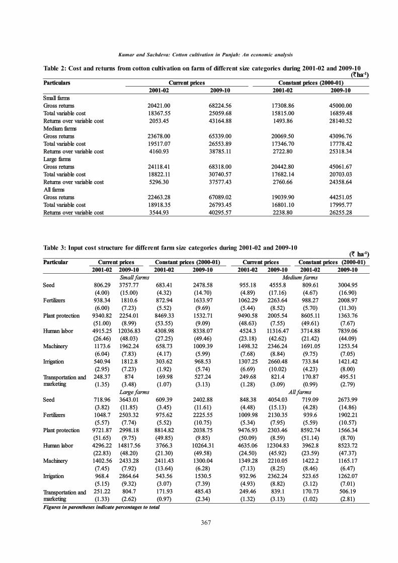
367
Kumar and Sachdeva: Cotton cultivation in Punjab: An economic analysis
Table 3: Input cost structure for different farm size categories during 2001-02 and 2009-10(` ha-1)
Particular Current prices Constant prices (2000-01) Current prices Constant prices (2000-01)2001-02 2009-10 2001-02 2009-10 2001-02 2009-10 2001-02 2009-10
Small farms Medium farmsSeed 806.29 3757.77 683.41 2478.58 955.18 4555.8 809.61 3004.95
(4.00) (15.00) (4.32) (14.70) (4.89) (17.16) (4.67) (16.90)Fertilizers 938.34 1810.6 872.94 1633.97 1062.29 2263.64 988.27 2008.97
(6.00) (7.23) (5.52) (9.69) (5.44) (8.52) (5.70) (11.30)Plant protection 9340.82 2254.01 8469.33 1532.71 9490.58 2005.54 8605.11 1363.76
(51.00) (8.99) (53.55) (9.09) (48.63) (7.55) (49.61) (7.67)Human labor 4915.25 12036.83 4308.98 8338.07 4524.3 11316.47 3714.88 7839.06
(26.46) (48.03) (27.25) (49.46) (23.18) (42.62) (21.42) (44.09)Machinery 1173.6 1962.24 658.73 1009.39 1498.32 2346.24 1691.05 1253.54
(6.04) (7.83) (4.17) (5.99) (7.68) (8.84) (9.75) (7.05)Irrigation 540.94 1812.8 303.62 968.53 1307.25 2660.48 733.84 1421.42
(2.95) (7.23) (1.92) (5.74) (6.69) (10.02) (4.23) (8.00)Transportation andmarketing
248.37 874 169.98 527.24 249.68 821.4 170.87 495.51(1.35) (3.48) (1.07) (3.13) (1.28) (3.09) (0.99) (2.79)
Large farms All farmsSeed 718.96 3643.01 609.39 2402.88 848.38 4054.03 719.09 2673.99
(3.82) (11.85) (3.45) (11.61) (4.48) (15.13) (4.28) (14.86)Fertilizers 1048.7 2503.32 975.62 2225.55 1009.98 2130.35 939.6 1902.21
(5.57) (7.74) (5.52) (10.75) (5.34) (7.95) (5.59) (10.57)Plant protection 9721.87 2998.18 8814.82 2038.75 9476.93 2303.46 8592.74 1566.34
(51.65) (9.75) (49.85) (9.85) (50.09) (8.59) (51.14) (8.70)Human labor 4296.22 14817.56 3766.3 10264.31 4635.06 12304.83 3962.8 8523.72
(22.83) (48.20) (21.30) (49.58) (24.50) (45.92) (23.59) (47.37)Machinery 1402.56 2433.28 2411.43 1300.04 1349.28 2210.05 1422.2 1165.17
(7.45) (7.92) (13.64) (6.28) (7.13) (8.25) (8.46) (6.47)Irrigation 968.4 2864.64 543.56 1530.5 932.96 2362.24 523.65 1262.07
(5.15) (9.32) (3.07) (7.39) (4.93) (8.82) (3.12) (7.01)Transportation andmarketing
251.22 804.7 171.93 485.43 249.46 839.1 170.73 506.19(1.33) (2.62) (0.97) (2.34) (1.32) (3.13) (1.02) (2.81)
Figures in parentheses indicate percentages to total
Table 2: Cost and returns from cotton cultivation on farm of different size categories during 2001-02 and 2009-10(`ha-1)
Particulars Current prices Constant prices (2000-01)2001-02 2009-10 2001-02 2009-10
Small farmsGross returns 20421.00 68224.56 17308.86 45000.00Total variable cost 18367.55 25059.68 15815.00 16859.48Returns over variable cost 2053.45 43164.88 1493.86 28140.52Medium farmsGross returns 23678.00 65339.00 20069.50 43096.76Total variable cost 19517.07 26553.89 17346.70 17778.42Returns over variable cost 4160.93 38785.11 2722.80 25318.34Large farmsGross returns 24118.41 68318.00 20442.80 45061.67Total variable cost 18822.11 30740.57 17682.14 20703.03Returns over variable cost 5296.30 37577.43 2760.66 24358.64All farmsGross returns 22463.28 67089.02 19039.90 44251.05Total variable cost 18918.35 26793.45 16801.10 17995.77Returns over variable cost 3544.93 40295.57 2238.80 26255.28
368
Indian J Econ Dev 12 (2): 2016 (April-June)
(24.50 percent) followed by machine labor `1349.28(7.13 percent), fertilizers `1009.98 (5.34 percent) andseed `848.38 (4.48 percent) per ha. Bt-cotton, requiringlesser number of plant protection sprays due to its pestresistant characteristics, covered most of the cottongrowing area of the state by the year 2009-10. Amongthe total variable cost in 2009-10, the major share was ofhuman labor (45.92 percent) as picking is a labor intensiveoperation and is still done manually. Due to higher yieldadvantage, picking in Bt- cotton required more labor. Thecost incurred on seed was `4054.03 per ha (15.13percent) followed by irrigation Rs. 2362.24 (8.82 percent),plant protection `2303.46 (8.59 percent), machine labor`2210.05 (8.25 percent) and fertilizers `2130.35 (7.95percent).
It can be seen from the Table 3 that during 2001-02, the selected cultivators incurred maximum cost onplant protection. Whereas, during 2009-10 the farmersincurred maximum cost on human labor. The requirementof fertilizers and irrigation for Bt-cotton was more ascompared to non-Bt cotton. However, the plant protectioncost for Bt-cotton was much lesser than that of non-Btcotton.
At constant prices of 2000-01 the cost of seed whichwas `719.09 per hectare in 2001-02 increased to `2673.99per hectare during 2009-10. Similarly, cost of fertilizersincreased from `939.60 to `1902.21 and irrigationincreased from `523.65 to `1262.07 per ha during thesame period. However, cost of plant protection whichwas as high as `8592.74 per hectare during 2001-02declined to `1566.34 per ha during 2009-10.
CONCLUSION AND POLICY IMPLICATIONSSeed of Bt-cotton hybrid is costly and farmer has
to purchase it from market every year. During 2009-10around 15 percent of the total variable cost was incurredon seed by the sampled farmers. So, the governmentshould take pre-requisite administrative steps in providingquality seed in each possible market, ensuring the quality,in league with the state agriculture agencies. Thegovernment may provide quality Bt seed to small andmarginal farmers at subsidized prices though cooperativesand state agriculture department. Cotton picking is a labourintensive operation and is still done by human labour. So,during picking time farmers face shortage of labour andforced to hire human labour at higher rates. During 2009-10, about 46 percent of the total variable cost was spenton hiring human labour by the sampled farmers.Mechanization of picking operation can provide solutionto this problem. So, research should be focused ondeveloping the mechanical pickers for cotton picking.REFERENCESAnonymous. 2013. Statistical abstracts of Punjab. Economic
and Statistical organization, Chandigarh.Anonymous. 2014. http://www.statista.com/263055/cotton-
production-worldwide-by-top-countries/Anonymous. 2014a. http://www.indiastat.com/table/
agriculture/2/cotton/17205/17400/data.aspxAnonymous. 2015. Cotton monthly research report. Culled
from http://www.agriwatch.com.Bennett, R.M., Ismael,Y., Kambhampati, U. and Morse, S.
2004. Economic impact of genetically modified cotton inIndia. Ag Bio Forum. 7: 96-100.
*This article forms a part of M.Sc. Thesis of the first author submitted to the Punjab Agricultural University, Ludhiana

369
www.soed.in
Entrepreneurial Behaviour of Vegetable Growers inKarnatakaN. Kumara*, A. Nehal Farooquee, and P.V.K.Sasidhar
School of Extension and Development Studies, IGNOU, New Delhi (110068)
*Corresponding author’s email: [email protected]
Received: November 24, 2015 Accepted: March 25, 2016
Indian Journal of Economics and DevelopmentVolume 12 No. 2: 369-376
April-June, 0000DOI: 10.5958/2322-0430.2016.00150.5
ABSTRACTThis study has attempted to investigate entrepreneurial behaviour of vegetable growers and the factors contributingtowards entrepreneurial behavior and its association with their personal and socio-economic traits. The importantfindings of the study were: majority (41 percent) of farmers had medium entrepreneurial behaviour followed by low (39percent) and high level (19 percent) of Entrepreneurial behavior.A positive and significant relationship was observedbetween entrepreneurial behaviour of farmers and their personal, socio-economic and psychological characteristicssuch as education, land holding, social participation, mass media participation, extension participation, level of aspirationand adoption. It was found that the most important components of entrepreneurial behaviour were information seekingbehaviour, innovativeness, farm decision making, and assistance of management service and achievement motivation.
KeywordsVegetable grower, entrepreneur, farm decision, innovative, risk taking, knowledge
JEL CodesA13, D80, L10, L53, Q10, Q13
INTRODUCTIONVegetables constitute about 55 percent of
horticultural crop production in the country with a totalproduction of 85 million tonnes which is estimated tocross 100 million tonnes in near future. Vegetable growingnot only provides continuous income and improves dietarystandards of family, but also supplements the income andreduces unemployment to a large number of the ruralpoor. Vegetables play a significant role in human nutritionespecially as a source of vitamin, minerals and traceelements apart from being the major supplier of dietaryfibre. ICMR has recommend a daily intake of 275 gm ofvegetables per adult per day, however actual consumptionless than 100 gm.
In vegetables production, India is next only to Chinawith an annual production of 87.53 million tonnes from5.86 million hectares having a share of 14.4 percent tothe world production. Karnataka stands 5th position inarea and production of vegetable crops. Horticulture cropsoccupy an area of 17.25 lakh hectares in the State. TheState produces 12 percent of total fruits and 8 percent oftotal vegetables grown in the country. 2010-11 vegetables
occupy an area of 4.38 lakh ha with production of 73.80million tonnes of Vegetables with growth rate of 10.0percent in production with a growth rate in area of 6.1percent (Karnataka State Horticulture Department).
Entrepreneurship stands as a vehicle to improve thequality of life for individuals, families and communitiesand to sustain a healthy economy and environment.(Petrin, 1994.). An entrepreneur is someone whoproduces for the market. An entrepreneur is a determinedand creative leader, always looking for opportunities toimprove and expand his business. An entrepreneur likesto take calculated risks, and assumes responsibility forboth profits and losses. An entrepreneur is passionateabout growing his business and is constantly looking fornew opportunities.Entrepreneurs are also innovators.They always look for better and more efficient andprofitable ways to do things. Being innovative is animportant quality for a farmer-entrepreneur, especiallywhen the business faces strong competition or operatesin a rapidly changing environment (Kahan, 2012).Farmersthose who are progressive cannot be identified asagricultural entrepreneurs but those who are entrepreneurs
370
Indian J Econ Dev 12 (2): 2016 (April-June)
are essentially progressive farmers. The entrepreneur isan economic man, who strives to maximize his profitsby innovations. He is a man with a will to act, to assumerisk and to bring about a change through organization ofhuman efforts.
India has immense potential for entrepreneurshipdevelopment in terms of diversity of rural occupations.Vegetable production is one of the promising sectors ofentrepreneurship development in India. Development ofentrepreneurship ensures optimal utilization of resourcesand facilities and value addition to product and services.It also helps in developing capability to cope up with theimpact of globalization. There are many factors thatinfluence the entrepreneurial behaviour of human beings.According to Amarnath and Samvel (2008) the emergenceof entrepreneurs in a society depends upon closelyinterlinked social, religious, cultural, psychological andeconomic factors. Understanding the role of these factorsis essential for creating an environment which canfacilitate the development of entrepreneurial behaviour.
Entrepreneurial behavior can be attributed as thechange in knowledge, skills and attitude of entrepreneursin the enterprise they have taken up. In the presentscenario, entrepreneurship development in agriculture andfood sector is a key driver for promoting and sustainingthe momentum of growth and providing employment. Inthis backdrop, this study has aimed to investigate theentrepreneurial behavior of vegetable growers, the factorscontributing towards entrepreneurial behavior and itsassociation with their personal and socio-economic traitswere taken up.METHODOLOGY
The present study was conducted in four villagesof kadur and chikmagalore talukas of chickmagaloredistrict of Karnataka state during June 2014 to April 2015and study site classified under central dry zone, liesbetween 12 54’ and 13 53’ North latitude and 75 04’ and76 21’ East longitudes receives annual rainfall of about1925 mm with maximum temperature of 31 C andminimum of 14 C.
Random sampling technique with purposive selectionwas employed to select 100 vegetable growers. Therewere three categories based on their Land Holdings. Thus85 small farmers (1-2 Ha), 12 medium farmers (2-5 Ha)and 3 large farmers (5 ha above) (90 were Male & 10were female) were taken as respondents. The data wascollected through personal interview and was analyzedby using suitable statistical techniques.
Entrepreneurial behaviour was taken as a functionof ten components viz., innovativeness, farm decisionmaking, achievement motivation, and knowledge offarming enterprise, risk taking ability, information seekingbehaviour, ability to co-ordinate farm activities, assistance
of management service, leadership ability andcosmopoliteness. The summation of scores of all theseten components constitutes the entrepreneurial behaviourScore of the respondents. The ten selected componentsof entrepreneurial behaviour were measured by using thefollowing methods.Innovativeness: Innovativeness was operationallydefined as the degree to which an individual adopts newideas relatively earlier than others in his social system(Rogers and Svenning, 1969).The scale developed by Rao(1985) with suitable modifications was used to measureinnovativeness of respondents. For measuringinnovativeness of respondents, the most importantvarieties and practices recommended during last 5 to 10years were selected in consultation with farmers,extension workers of the study area. There were eightitems in the scale and nine th item was kept open for anyother new practice adopted by the respondents applicableto them. A score of one was given for each year from thetime the respondent first adopted that particular practicetill 2004. Summated score over all the items over yearsof adoptionFarm decision making: The decision making ability ofa farmer is operationally defined as the degree of weighingthe available alternatives in terms of their desirability andtheir likelihoods and choosing the most appropriate onefor achieving maximum profit on his farming. The scaledeveloped by Supe (1969), which was also adopted byRao (1985) with modifications was found to be moreappropriate to measure decision making ability of farmers.Hence, it was used in the present study with suitablemodification. The original scale of Supe (1969) containedeight items on package of practices for cotton crop. Theseitems were modified for measuring the decision makingin choosing the different alternatives of package ofpractices in general. The weight ages of 3, 2 and 1 assuggested by Supe (1969) were assigned to the threerationality levels namely ‘rational’, ‘inter mediate’ and ‘lessrational’, respectively. Thus, the possible score for eachfarmer on his decision making ability ranged from 7 to21.Based on the total score obtained by respondents ondecision making, they were grouped into following threecategories, keeping the mean and standard deviation ascheck.Low : <X – 1/2 SD,Medium : X + 1/2 SD,High :>X + 1/2 SDAchievement motivation: Achievement motivation isimportant to excel in one’s personal life, community orsocial work and to influence the environment is very muchneeded to achieve development (Sharma et al. (2008). Itwas operationalized as the desire for excellence to attaina sense of personal accomplishment. It was measuredwith the help of procedure adopted by Chandrapaul(1998).The instrument consisted of six statements and

371
Kumara et al.: Entrepreneurial behaviour of vegetable growers in Karnataka
responses obtained on three point continuum namely‘agree’, ‘undecided’ and ‘disagree’. A weightage of 3, 2and 1, respectively were assigned to the responsecategories in the case of positive statements and thescoring was reversed for negative statements. The totalscore of the respondents on their achievement motivationwas arrived summing up the weightages of responsesfor each statement. Thus, the total score for each farmeron his achievement motivation ranged from 6 to 18.Basedon the total score obtained by respondents onachievement motivation, they were grouped into threecategories, keeping the mean and standard deviation ascheck.Low : <X – 1/2 SD,Medium : X + 1/2 SD, High :>X + 1/2 SDKnowledge of farming enterprise: It is the degree towhich the factual information is possessed by therespondent regarding the farming enterprise. In thepresent study, knowledge of farming enterprise wasmeasured with the help of a scale developed byVenkataramaiah (1991) with suitable modifications byusing rating scale which consists of ‘Yes’ and ‘No’ typeof questions. The ‘Yes’ item was scored by giving onepoint and zero if respondent has not answered correctly.The maximum score on this scale was 10. Based on thetotal score obtained by the respondents on knowledge offarming enterprise, they were grouped into threecategories, keeping the mean and standard deviation ascheck .Low : <X – 1/2 SD, Medium : X + 1/2 SD, High: >X + 1/2 SDRisk taking ability: Risk taking ability wasoperationalized as the degree to which the farmer isoriented towards risk and uncertainty in facing problemsin farming. In the present study, risk taking ability ofrespondents was measured with the help of a scaledeveloped by Supe (1969). The scale contained sixstatements of which first and fifth statements werenegatively keyed. Modification in the scoring procedurewas made by giving a weightage of 2 for the ‘Yes’ responseand 1 for ‘No’ response for positive statement. This wasreversed in case of negative statements. The aggregateof weights over six statements was the total score of arespondent on this variable. The possible score range wasfrom 6 to 12. Based on the total score obtained by therespondents on risk taking ability, they were grouped intothree categories, keeping the mean and standard deviationas check.Low : <X – 1/2 SD, Medium: X + 1/2 SD, High: >X + 1/2 SD
Information seeking behavior; Informationseeking was operationally defined as the frequency ofcontact or exposure of a farmer to different sources forobtaining farm information. The information seekingbehaviour of a farmer was measured with rating scale
developed by Rao (1985). The scale contains 16 itemsand were categorized under three sub-heads namelyinformal sources, formal sources and mass media. Fordetermining the degree of information seeking by therespondents through these sources, four responsecategories namely frequently, occasionally, rarely andnever were provided with weight ages 3, 2, 1 and 0,respectively. Based on the score obtained by respondentson information seeking, they were grouped into threefollowing categories, keeping the mean and standarddeviation as check. Low : <X – 1/2 SD, Medium: X + 1/2 SD, High : >X + 1/2 SDAbility to co-ordinate farm activities: It was definedas the degree to which an individual co-ordinates actionin a time dimension. The scale developed by Nandapurkar(1980) with suitable modifications was used to measurethe farmer’s ability to co-ordinate farm activities. Thescale consists of five questions. A score of 2, 1 and 0were assigned for the responses “well in advance”, “atthe nick of time” and “don’t consider” respectively. Totalscore was obtained by summing up the scores recorded.Thus the maximum and minimum possible score was 10and 0 respectively. Based on the score obtained byrespondents on their ability to coordinate farm activities,they were grouped into three categories, keeping the meanand standard deviation as check. Low : <X – 1/2 SD,Medium: X + 1/2 SD, High : >X + 1/2 SDAssistance of management service: It refers to thedegree to which a farmer gets assistance of managementservice. The scale developed by Nandapurkar (1980) wasused to measure the assistance of management service.The scale contained 5 questions. A score of 2, 1 and 0were assigned for responses “always”, “Some times” and“never” respectively. Total score was obtained bysumming up the scores recorded. Thus maximum andminimum possible score for each respondent will be 10and 0 respectively. Based on the scores obtained byrespondents on assistance of management service, theywere grouped into three categories, keeping the meanand standard deviation as check. Low : <X – 1/2 SD,Medium: X + 1/2 SD, High : >X + 1/2 SDLeadership ability: Leadership ability was operationalizedas the degree to which an individual initiates or motivatesthe action of others. Scale developed by Nandapurkar(1980) with suitable modifications was used to measureleadership ability. In the present study, leadership abilitywas measured along a three point rating scale “Always”,“Some times” and “never” with decreasing score from2, 1 and 0 respectively. The total score was computedfor each respondent by summing up the scores recorded.Based on the total scores obtained, the respondents wereclassified into 3 categories, keeping the mean and standard

372
Indian J Econ Dev 12 (2): 2016 (April-June)
deviation as check. Low : <X – 1/2 SD, Medium: X + 1/2 SD, High : >X + 1/2 SDCosmo politeness: It was operationalized as the degreeto which a farmer is oriented outside his community orvillage that might make him more accessible withinnovations. In the present study cosmopoliteness wasmeasured by using the procedure adopted by Nandapurkar(1980) and Venkataramaiah (1991). The scale consistsof three statements. The responses were obtained andscores were given in terms of 1 for ‘Yes’ and 0 for ‘No’.The total score was computed by summing up all thescores recorded based on the total scores obtained, therespondents were classified into 3 categories, keepingthe mean and standard deviation as check. Low : <X – 1/2 SD, Medium: X + 1/2 SD, High : >X + 1/2 SDRESULTS AND DISCUSSIONPersonal, Socio-economic and PsychologicalFharacteristics of FarmersAge: It is apparent from Table 1 that majority of therespondents (44 percent) were under middle age categoryfollowed by young age (36 percent) and old age (16.67percent) categories. Among categories majority (66.67percent) were old age group. Among the groups, 44.70percent of small farmers, 41 percent of medium farmersand 33.33 percent of big farmers were under middle agecategory, while small (37.64 percent), medium (33.33 v)farmers and zero per cent of big farmers were underyoung age category. The remaining 15.00 percent of smallfarmers, 25.00 percent of medium farmers and 66.67percent of big farmers were under old age category.
Table 1: Distribution of respondents according to theirage
(Percent)Category Farm category
Small(n1=85)
Medium(n2=12)
Large(n3=3)
Overall(n=100)
Young age (<35 years) 37.64 33.33 0.00 36.00Middle age (36-50 years) 44.70 41.00 33.33 44.00Old age (>50 years) 17.65 25.00 66.67 16.67Total 100.00 100.00 100.00 100.00
Education: It is clear from the Table 2 that majority (60.00percent) of small farmers, 16.66 percent of mediumfarmers were illiterates. The results revealed that 33.00and 50.00 percent of small and medium farmers wereeducated up to middle school, respectively. Only 2.50percent of small farmers, 16.66 percent of mediumfarmers and 33.33 percent of big farmers were educatedup to middle school. Around 7.50 percent of smallfarmers, 8.33 percent of medium farmers and 33.33percent of big farmers were educated up to high school.About 8.35 percent of medium farmers and 33.33 percentof big farmers were educated up to higher secondary
school, However, glance at sample as a whole indicatethat majority of respondents were illiterates 53 percentfollowed by education up to primary school, middleschool, high school, higher secondary school with 26.11,8.2, percent respectively.
Table 2: Distribution of respondents according to theireducation
(Percent)Category Farm category
Small(n1=85)
Medium(n2=12)
Large(n3=3)
Overall(n=100)
Illiterate 60.00 16.66 - 53.00Primary school 30.00 50.00 - 26.00Middle school 2.50 16.66 33.33 11.00Middle school 2.50 16.66 33.33 11.00High School 7.50 8.33 33.33 8.00Higher secondary school - 8.35 33.33 2.00Total 100.00 100.00 100.00 100.00
Occupation: The results from Table 3 indicated frompooled data that majority (69 percent) of the respondentswere dependent only on Farming (Agriculture,Horticulture). Whereas, 25 percent of respondents werepracticing agricultural and subsidiary enterprises like dairy,poultry and only 6 per cent of respondents werepracticing agricultural and subsidiary enterprises inaddition to other sources of income like business. Amongthe categories, majority (72.94 percent) of small farmers,medium (58.33 percent) were dependent only onagriculture, Horticulture followed by 23.52 percent ofsmall farmers, 25 percent of medium farmers and 66.64percent of big farmers practicing agricultural andsubsidiary enterprises. Whereas 3 percent of small farmers16.64 percent of medium farmers and 33.34 percent bigfarmers were practicing agricultural and subsidiaryenterprises in addition to other sources of income.
Table 3: Distribution of respondents according to theiroccupation
(Percent)Category Farm category
Small(n1=85)
Medium(n2=12)
Large(n3=3)
Overall(n=100)
Farming alone 72.94 58.33 0.00 69.00Farming + subsidiary 23.52 25.00 66.66 25.00Farming + subsidiary +others
3.54 16.64 33.34 6.00
Total 100.00 100.00 100.00 100.00
Land Holding; For the study purpose, Respondents werecategorized into three groups based on their land holdingand their distribution and as per Table 4, indicates 85percent were small farmers 12 percent were mediumfarmers and 3 percent were big farmers.

373
Kumara et al.: Entrepreneurial behaviour of vegetable growers in Karnataka
Table 4: Distribution of respondents according to theirland holdingCategory Frequency PercentSmall farmers (<5 acres) 85 85.00Medium farmers (5-10 acres) 12 12.00Big farmers (>10 acres) 3 3.00Total 100 100.00
Social participation: The findings from Table 5 showedthat majority (75 percent) of the respondents had lowsocial participation, followed by medium (19 percent)and high (6 percent) social participation, respectively.Among the categories, majority (78.82 percent) of smallfarmers, 66.66 percent of medium farmers had low socialparticipation. Whereas, 16.47 percent of small farmers,25 percent of the medium farmers and 66.67 percent ofbig farmers had medium social participation. And only4.71 percent of small farmers, 8.34 percent of mediumfarmers and 33.34 percent of big farmers had high socialparticipationMass media participation: It is evident from the Table5 that majority of small farmers (41.17 percent), mediumfarmers (41.66 percent) and big farmers (33.33 percent)had medium mass media participation. Whereas, equalper cent (30.60 percent, 33.34 percent and 33.33 percent)of small, medium and big farmers had low mass mediaparticipation. The remaining 28.23 percent of smallfarmers, 25.00 percent of medium farmers and 33.34percent of big farmers had high social participation. Theresults from pooled data indicated that majority (41percent) of the respondents belonged to medium massmedia participation category. Whereas, 31 and 28 percentof farmers belonged to low and high mass mediaparticipation categories, respectively.Extension participation: It is quite clear from the Table5 that majority (46 percent) of the respondents belongedto low extension participation category followed bymedium (34 percent) and high (20 percent) extensionparticipation categories, respectively. Among the groups,majority (66.67 percent) of big farmers, 48.24 percentof small farmers and 25 percent of medium farmers hadlow extension participation. While 32.94 percent of smallfarmers, 41.66 percent of medium farmers and 33.34percent of big farmers had medium extensionparticipation. Whereas, 18.82 percent of small, 33.34percent of medium farmers had high extensionparticipation.
Level of aspiration: The results from Table 5revealed that majority (45 percent) of the respondentshad medium level of aspiration followed by 34 and 21percent of respondents having low and high level ofaspiration, respectively. Among the categories, 44.71percent of small farmers, 41.66 percent of medium
farmers and 66.67 percent of big farmers had mediumlevel of aspiration followed by 35.29 percent of small, 25percent of medium and 33.33 percent of big farmershaving low level of aspiration. Whereas, 20.00 percentof small farmers, 33.34 percent of medium farmers hadhigh level of aspiration.Adoption of improved practices: It is evident from theTable 5 that 41.17 percent of small farmers, 50 percenteach of medium farmer’s and 66.67 percent big farmershad medium level of adoption. Whereas, 34.12 percentof small farmers, 25 percent of medium farmers had lowlevel of adoption. Further, high level of adoption wasobserved from big, medium and small farmers with 33.33,25.00 and 24.71 percent respectively. However, fromfindings it could be observed that 43 percent ofrespondents had medium level of adoption, 32 percenthad low level of adoption while 25 percent had high levelof adoption.
Table 5: Number of farmers in social participation, massmedia participation, extension participation, level ofaspiration and adoption level
(Percent)Category Farm category
Small(n1=85)
Medium(n2=12)
Large(n3=3)
Overall(n=100)
Social ParticipationLow 78.82 66.66 0.00 75.00Medium 16.47 25.00 66.66 19.00High 4.71 8.34 33.34 6.00Total 100.00 100.00 100.00 100.00Mass media participationLow 30.60 33.34 33.33 31.00Medium 41.17 41.66 33.33 41.00High 28.23 25.00 33.34 28.00Total 100.00 100.00 100.00 100.00Extension participationLow 48.24 25.00 66.67 46.00Medium 32.94 41.66 33.33 34.00High 18.82 33.34 0.00 20.00Total 100.00 100.00 100.00 100.00Level of aspirationLow 35.29 25.00 33.33 34.00Medium 44.71 41.66 66.67 45.00High 20.00 33.34 0.00 21.00Total 100.00 100.00 100.00 100.00Adoption levelLow 34.12 25.00 0.00 32.00Medium 41.17 50.00 66.67 43.00High 24.71 25.00 33.33 25.00Total 100.00 100.00 100.00 100.00
Entrepreneurial BehaviorThe summation of scores of all the ten selected
components constitutes the entrepreneurial Behaviourscore of the respondents.
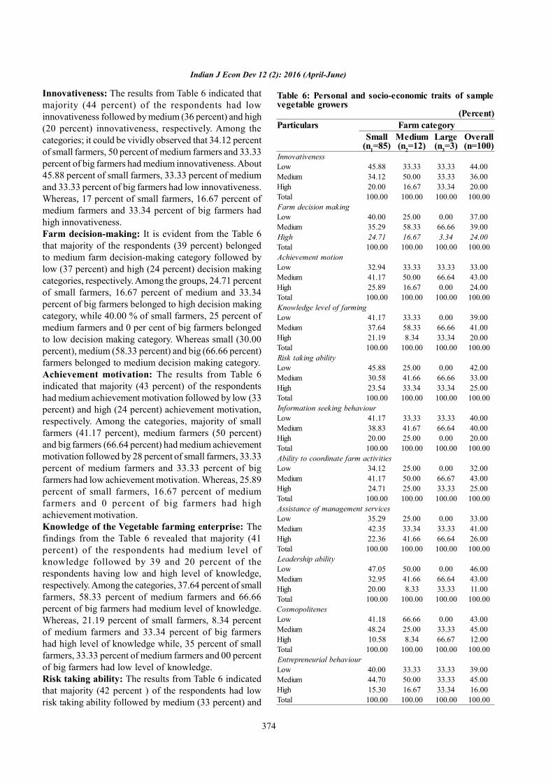
374
Indian J Econ Dev 12 (2): 2016 (April-June)
Innovativeness: The results from Table 6 indicated thatmajority (44 percent) of the respondents had lowinnovativeness followed by medium (36 percent) and high(20 percent) innovativeness, respectively. Among thecategories; it could be vividly observed that 34.12 percentof small farmers, 50 percent of medium farmers and 33.33percent of big farmers had medium innovativeness. About45.88 percent of small farmers, 33.33 percent of mediumand 33.33 percent of big farmers had low innovativeness.Whereas, 17 percent of small farmers, 16.67 percent ofmedium farmers and 33.34 percent of big farmers hadhigh innovativeness.Farm decision-making: It is evident from the Table 6that majority of the respondents (39 percent) belongedto medium farm decision-making category followed bylow (37 percent) and high (24 percent) decision makingcategories, respectively. Among the groups, 24.71 percentof small farmers, 16.67 percent of medium and 33.34percent of big farmers belonged to high decision makingcategory, while 40.00 % of small farmers, 25 percent ofmedium farmers and 0 per cent of big farmers belongedto low decision making category. Whereas small (30.00percent), medium (58.33 percent) and big (66.66 percent)farmers belonged to medium decision making category.Achievement motivation: The results from Table 6indicated that majority (43 percent) of the respondentshad medium achievement motivation followed by low (33percent) and high (24 percent) achievement motivation,respectively. Among the categories, majority of smallfarmers (41.17 percent), medium farmers (50 percent)and big farmers (66.64 percent) had medium achievementmotivation followed by 28 percent of small farmers, 33.33percent of medium farmers and 33.33 percent of bigfarmers had low achievement motivation. Whereas, 25.89percent of small farmers, 16.67 percent of mediumfarmers and 0 percent of big farmers had highachievement motivation.Knowledge of the Vegetable farming enterprise: Thefindings from the Table 6 revealed that majority (41percent) of the respondents had medium level ofknowledge followed by 39 and 20 percent of therespondents having low and high level of knowledge,respectively. Among the categories, 37.64 percent of smallfarmers, 58.33 percent of medium farmers and 66.66percent of big farmers had medium level of knowledge.Whereas, 21.19 percent of small farmers, 8.34 percentof medium farmers and 33.34 percent of big farmershad high level of knowledge while, 35 percent of smallfarmers, 33.33 percent of medium farmers and 00 percentof big farmers had low level of knowledge.Risk taking ability: The results from Table 6 indicatedthat majority (42 percent ) of the respondents had lowrisk taking ability followed by medium (33 percent) and
Table 6: Personal and socio-economic traits of samplevegetable growers
(Percent)Particulars Farm category
Small(n1=85)
Medium(n2=12)
Large(n3=3)
Overall(n=100)
InnovativenessLow 45.88 33.33 33.33 44.00Medium 34.12 50.00 33.33 36.00High 20.00 16.67 33.34 20.00Total 100.00 100.00 100.00 100.00Farm decision makingLow 40.00 25.00 0.00 37.00Medium 35.29 58.33 66.66 39.00High 24.71 16.67 3.34 24.00Total 100.00 100.00 100.00 100.00Achievement motionLow 32.94 33.33 33.33 33.00Medium 41.17 50.00 66.64 43.00High 25.89 16.67 0.00 24.00Total 100.00 100.00 100.00 100.00Knowledge level of farmingLow 41.17 33.33 0.00 39.00Medium 37.64 58.33 66.66 41.00High 21.19 8.34 33.34 20.00Total 100.00 100.00 100.00 100.00Risk taking abilityLow 45.88 25.00 0.00 42.00Medium 30.58 41.66 66.66 33.00High 23.54 33.34 33.34 25.00Total 100.00 100.00 100.00 100.00Information seeking behaviourLow 41.17 33.33 33.33 40.00Medium 38.83 41.67 66.64 40.00High 20.00 25.00 0.00 20.00Total 100.00 100.00 100.00 100.00Ability to coordinate farm activitiesLow 34.12 25.00 0.00 32.00Medium 41.17 50.00 66.67 43.00High 24.71 25.00 33.33 25.00Total 100.00 100.00 100.00 100.00Assistance of management servicesLow 35.29 25.00 0.00 33.00Medium 42.35 33.34 33.33 41.00High 22.36 41.66 66.64 26.00Total 100.00 100.00 100.00 100.00Leadership abilityLow 47.05 50.00 0.00 46.00Medium 32.95 41.66 66.64 43.00High 20.00 8.33 33.33 11.00Total 100.00 100.00 100.00 100.00CosmopolitenesLow 41.18 66.66 0.00 43.00Medium 48.24 25.00 33.33 45.00High 10.58 8.34 66.67 12.00Total 100.00 100.00 100.00 100.00Entrepreneurial behaviourLow 40.00 33.33 33.33 39.00Medium 44.70 50.00 33.33 45.00High 15.30 16.67 33.34 16.00Total 100.00 100.00 100.00 100.00

375
Kumara et al.: Entrepreneurial behaviour of vegetable growers in Karnataka
high (25 percent) risk taking ability, respectively. Amongthe groups, majority (45.88 percent) of small farmers,25 percent of medium farmers had low risk taking abilityfollowed by 23.54 percent of small farmers, 33.34 percentof medium farmers and 33.34 percent of big farmershaving high risk taking ability. Whereas, 26 percent ofsmall farmers, 41.66 percent of medium farmers and66.66 percent of big farmers had medium risk takingability.Information seeking behavior: It could be inferredfrom the Table 6 that majority (40 percent) of therespondents had medium and low information seekingbehaviour followed by low (20 percent) informationseeking behavior categories. Among the categories, it isobserved that 38.83 percent of small farmers, 41.67percent of medium farmers and 66.64 percent of bigfarmers had medium information seeking behaviour.Whereas, 41.17 percent of small farmers, 33.33 percentof medium farmers and 33.33 percent of big farmershad low information seeking behavior, while 20.00 percentof small farmers, 25 percent of medium farmers and 0percent of big farmers had high information seekingbehaviour.Ability to co-ordinate farm activities: It is apparentfrom Table 6 that maximum (43 percent) of mediumfarmers had medium ability to co-ordinate farm activitiesfollowed by 32 percent of small farmers, and 25 percentof big farmers. 24.71 percent of small farmers 25 percentof medium farmers and 25 percent of big farmers havinghigh ability to co-ordinate farm activities. Whereas small(34.12 percent), medium (25 percent) farmers and 00percent of big farmers had low ability to co-ordinate farmactivities. Overall, majority (43 percent) of therespondents had medium ability to co-ordinate farmactivities.Assistance of management service: From Table 6, itis evident that majority (41 percent) of the respondentshad medium assistance of management service followedby low (33 percent) and high (26 percent) assistance ofmanagement service, respectively. Among the groups,42.35 percent of small farmers, 33.34 percent of mediumfarmers and 33.33 percent of big farmers had mediumassistance of management service. Whereas, 35.29percent of small farmers, 25 percent of medium farmershad low assistance of management service. And 22.36percent of small farmers, 41.66 percent of mediumfarmers and 66.64 percent of big farmers had highassistance of management service.Leadership ability: The findings from Table 6 showedthat majority (46 percent) of the respondents had lowlevel of leadership ability followed by medium (35 percent)and high (19 percent) level of leadership abilityrespectively. Among the categories, majority of small
farmers (47.05 percent), medium farmers (50 percent)had low level of leadership ability followed by 32.95percent of small farmers, 41.66 percent of mediumfarmers and 66.64 percent of big farmers having mediumlevel of leadership ability. Whereas, 20.00 percent of smallfarmers, 8.33 percent of medium farmers and 33.33percent of big farmers had high level of leadership ability.Cosmo politeness: From the Table 6, it is observed thatmajority (45 percent) of the respondents had mediumlevel of cosmopoliteness followed by low (43 percent)and high (12 percent) level of cosmopoliteness,respectively. Among the categories majority (66.67percent) of big farmers had high level of cosmopoliteness.It is observed that 48.24 percent of small farmers, 25percent of medium farmers and 33.33 percent of bigfarmers had medium level of cosmopoliteness. Whereas,majority (66.66 percent) of medium farmers, 41.18percent of small farmers had low level of cosmopoliteness.And 10.58 percent of small farmers, 8.34 percent ofmedium farmers and 66.67 percent of big farmers hadhigh level of cosmopoliteness.Entrepreneurial behavior: The summation of scoresof all the ten selected components constitutes theentrepreneurial behaviour score of the respondents. Itwas apparent from Table 6 that 40 percent of smallfarmers, 33.33 percent of medium farmers and 33.33percent of big farmers had low level of entrepreneurialbehaviour. Whereas, 44.70 percent of small farmers, 50percent of medium farmers and 33.33 percent of bigfarmers had medium level of entrepreneurial behaviour,while 15.30 percent of small farmers, 16.67 percent ofmedium farmers and 33.33 percent of big farmers hadhigh level of entrepreneurial behaviour. A glance at thesample as a whole indicated that majority (45 percent) ofthe respondents belonged to medium entrepreneurialbehaviour category, whereas 39 percent were in lowentrepreneurial behaviour category and 16 percent of therespondents were in high entrepreneurial behaviourcategory.CONCLUSIONS
The data revealed that in case of small and mediumfarmers, majority of them had medium entrepreneurialbehaviour followed by low level. In case of large farmers,majority of them had high entrepreneurial behaviourfollowed by medium level. Large farmers because of theirresource richness and high risk taking ability had higherentrepreneurial behaviour than the small and mediumfarmers. Hence special consideration is required to developenterpreunarship in vegetable farmers. The entrepreneurbehavior was positively and significantly related witheducation of the respondent, land holding, materialpossession, economic status, social participation,economic motivation, marketing orientation, extension
376
Indian J Econ Dev 12 (2): 2016 (April-June)
agency contact and mass media communication.REFERENCESAmaranth, J.S. and Samvel, A.P.V. 2008. Agri business
management. Satish Serial Publishing House, Delhi.Chandrapaul, K. 1998. A study on entrepreneurial behaviour
of growers in Krishna district of Andhra Pradesh. M.Sc.(Agri.) Thesis submitted to Acharya N.G. RangaAgricultural University, Hyderabad.
Kahan, D. 2012. Entrepreneurship in farming. Food andAgriculture Organization, United Nations, Rome.
Nandapurkar, G.G., 1980. A study of the entrepreneurialbehavior of small farmers. Ph.D. Thesis submitted toU.A.S., Bangalore.
Petrin,T. 1994. Entrepreneurship as an economic force in rural
development. Keynote paper presented at the SeventhFAO/REU International Rural Development SummerSchool, Herrsching, Germany 8-14.
Rogers, E.M. and Svenning, L. 1969. Modernization amongPeasants. Holt McDougal, Rigby (US).
Sharma A.K , Rao, U.M.D., and Singh, L. 2008. Achievementmotivation in vegetable growers. Indian ResearchJournal of Extension Education. 8: 79-82.
Supe, S.V. 1969. Factors related to different degrees ofnationality indecision making among Farmers. Ph.D.Thesis sumitted to IARI, New Delhi.
Venkataramaiah, P. 1991. Development of socio-economicstatus scale for farm families of North Karnataka. Ph.D.Thesis submitted to University of Agricultural Sciences,Bangalore, Karnatka.

377
Determinants of Participation of Dairy Farmers in DairyCooperative Societies in ManipurL. Priscilla*, A.K. Chauhan, Lalrinsangpuii, and Bulbul G. Nagrale1Dairy Economics, Statistics and Management Division, ICAR-National Dairy Research Institute, Karnal
*Corresponding author’s email: [email protected]
Received: February 15, 2016 Accepted: March 10, 2016
Indian Journal of Economics and DevelopmentVolume 12 No. 2: 377-379
April-June, 2016DOI: 10.5958/2322-0430.2016.00151.7
www.soed.in
ABSTRACTThe study was conducted in Manipur state to study the determinants of dairy farmers’ participation in Dairy CooperativeSocieties (DCS). Four districts were selected purposively from the state and a sample of 240 milk producing householdswas drawn (120 members and 120 non-members). The primary data was collected on various variables and analysedusing Logistic regression technique. The results of the regression showed that average annual milk production, years offarming experience and distance to market were the important variables (significant at one percent) favourably influencinga dairy farmers participation in DCS. This implies that farmers having higher average annual milk production and moreexperience in dairy farming are more likely to participate in DCS. Also, greater the distance to market, higher thetransaction costs for the farmers which makes them favour participation in DCS located in their villages. Number ofdependents and size of landholding adversely affected (significant at 10 percent) participation meaning that farmers withlarger family size and also those with smaller landholding were more likely to participate in DCS.
KeywordsManipur, dairy cooperative societies, determinants, logistic regression
JEL CodesC81, D22, J54, Q13
INTRODUCTION:The dairy sector occupies an important place in the
Indian economy which is evident from the fact that milkis the second largest agricultural commodity contributingto GNP of the country, next only to rice. Dairying isrecognized as suitable for employment generation andvalue addition in the agricultural sector in the Indianeconomy in general and for rural families, especially, smalland marginal farmers and landless agricultural labourersin particular. During 2013-14, milk production was at arecord high of 137.69 Mt, thus becoming an importantsecondary source of income for 70 million ruralhouseholds engaged in dairying. The average year on yeargrowth rate of milk, at 4.18 per cent vis-à-vis the worldaverage of 2.2 per cent shows sustained growth inavailability of milk and milk products for the growingpopulation (Anonymous, 2015). The success of OperationFlood programme and AMUL paved the way for
cooperative movement and gave a momentum for dairydevelopment in almost all the states of the country. But inManipur, the dairy sector is far from realizing its potential.The total milk production of the state was 80.0 thousandtonnes during the year 2012-13 which was one of thelowest in the country. In spite of having the highestnumber of Dairy Cooperative Societies compared to theother North-East states (National Cooperative Union ofIndia, 2007-08), the per capita availability of milk isstagnant over the years, which was was 80 g/day during2010-11. This is far behind the national average of 281gm/day and WHO recommendation of 282 g/day(Anonymous, 2012). Consumption of milk and milkproducts is lower due to food habit and less availabilityof milk. However, increase in per capita income andchanges in life style are leading to an increase in demandfor milk and milk products in the state. The state haswitnessed a steady increase in milk production over the

378
Indian J Econ Dev 12 (2): 2016 (April-June)
yearsJoining dairy cooperatives have been found to be
beneficial to the members by many authors, such as thatof Kumar and Sharma (1999), Bihar; Meena (2008),Rajasthan; Singh (2012), Meghalaya in their studies.However, literature relating to the field of dairy is verylimited for the state of Manipur since a very limitedresearch has been done in this state till now. It will beessential to explore why some dairy farmers do not jointhe dairy cooperatives even though it is found that acrossthe country. Hence, the present study attempts to studythe factors which determine the participation of dairyfarmers in the cooperative societies in the state.METHODOLOGY
The present study was conducted in Manipur stateto study the determinants of dairy farmers’ participationin DCS. Out of the nine districts of Manipur, four districts,viz., Imphal East, Thoubal, Senapati and Churachandpurwere selected purposively from the state on the basis ofnumber of functioning DCS. From each district, one blockwas selected randomly. Three DCS was selectedrandomly from each of the four blocks making a total oftwelve DCS. A list of households having at least onelactating animal was prepared for each selected society.Then, a total of 120 milk producer members and 120non-members of similar socio-economic status wereselected from the same villages of member householdsmaking the total sample size of 240. To find out thedeterminants of participation by dairy farmers in DCS,primary data was collected on various variables.
A Logit model was used recognizing the discretechoice nature of the dependent variable as previously usedby Karli et al. (2006). The model postulates that Pb”, theprobability that ithdairy farmer joins the DCS, is a functionof an index variable Zi, summarizing a set of explanatoryvariables. Zi is equal to the logarithm of the odds ratio,i.e., the ratio of probability that a dairy farmer would jointhe DCS to the probability that he would not join it. Zi isexpressed as a linear function of explanatory variablesXi. Mathematically, the logit model is expressed as:
iziii eXFZFP
1
1)()(
m
k kiki
ii X
PPZ
11ln
Where, Pi = Probability that i th farmer would be a member of DCS i = 1, 2,…., 240= Number of dairy farmers
k = 1, 2,….,9 = Number of explanatory variables = Constant = Unknown parameter
The parameters of the model will be estimated usingthe maximum likelihood method. The index variable Zb”indicating whether a dairy farmer joins a cooperative ornot, will be a linear combination of a set of explanatoryvariables and the functional form can be written as:
Zi= + 1 X 1i+ 2X 2i+ 3 X 3i+……..+ 9 X 9iThe description of the variables is given below:
Explanatory variables MeasurementX 1 Age of respondents YearX 2 Education level 0 = Illiterate
1= Primary2 = Secondary3 = Higher secondary4 = University
X 3 Marital status (Married = 1, Otherwise = 0)X 4 Number of
dependentsTotal number of dependentsper household
X 5 Self- employment inoff-farm activities
1 = Engaged in off-farmactivities0 = Otherwise
X 6 Total number of milchanimals owned
Number
X 7 Land holding AcresX8 Years of farming
experienceYears
X9 Distance to market km
RESULTSAND DISCUSSIONThe results of the logistic regression are presented
in Table 1. A perusal of the Table 1 reveals that averageannual milk production, years of farming experience anddistance to market were the important variables(significant at one percent) favourably influencing a dairyfarmers participation in DCS. This implies that farmershaving higher average annual milk production and moreexperience in dairy farming are more likely to participatein DCS. Also, greater the distance to market, higher thetransaction costs for the farmers which makes themfavour participation in DCS located in their villages.Number of dependents and size of landholding adverselyaffected (significant at 10 percent) participation meaningthat farmers with larger family size and also those withsmaller landholding were more likely to participate in DCS.Farmers with larger landholding were found to mainlytake up crop cultivation as their main occupation andtherefore have lower participation in DCS.CONCLUSIONS
The study concluded that average annual milkproduction, years of farming experience and distance tomarket were the important variables (significant at onepercent) favourably influencing a dairy farmersparticipation in DCS. This implies that farmers having

379
higher average annual milk production and moreexperience in dairy farming are more likely to participatein DCS. Also, greater the distance to market, higher thetransaction costs for the farmers which makes themfavour participation in DCS located in their villages.Number of dependents and size of landholding adverselyaffected (significant at 10 percent) participation meaningthat farmers with larger family size and also those withsmaller landholding were more likely to participate in DCS.Farmers with larger landholding were found to mainlytake up crop cultivation as their main occupation andtherefore have lower participation in DCS.REFERENCESAnonymous. 2012. Basic animal husbandry statistics.
Department of Animal Husbandry, Dairying andFisheries, Ministry of Agriculture, Government of India,New Delhi
Anonymous. 2015. Economic survey 2014-15. Ministry ofFinance, Economic Division, Department of Economic
Affairs, Government of India, New Delhi.Karli, B., Bilgi, A., and Gill, Y. 2006. Factors affecting
farmers’decision to enter agricultural cooperatives usingRandom Utility Model in the South Eastern AnatolianRegion of Turkey. Journal of Agricultural and RuralDevelopment in Tropics and Subtropics. 107 (2): 115-127.
Kumar, R. and Sharma, A.K. 1999. Impact of dairy cooperativeson rural economy in Nalanda district. Journal ofDairying. Foods and Home Sciences. 18 (2): 92-97
Meena, G.L. 2008. Impact of dairy cooperatives on theeconomy of rural households in Alwar district ofRajasthan. Ph.D. Thesis submitted to National DairyResearch Institute (Deemed University), Karnal,Haryana.
Singh, R. 2012. Economic impact of integrated dairydevelopment project on rural households in MeghalayaState. Ph.D. Thesis submitted to National Dairy ResearchInstitute (Deemed University), Karnal, Haryana.
Priscilla et al.: Determinants of participation of dairy farmers in dairy cooperative societies in Manipur
Table 1: Determinants of dairy farmers' participation in dairy cooperative societiesVariables Estimated coefficients SEs p-valueConstant 2.841 1.311 0.03Age -0.015 0.023 0.53NS
Education 0.071 0.137 0.607NS
Marital status -0.402 0.367 0.274NS
Number of dependents -0.232 0.134 0.085*
Self employment in off-farm activities 0.471 0.388 0.225NS
Total number of milch animals 0.208 0.1 0.037**
Land Holding -0.5 0.272 0.067*
Years of farming experience 0.086 0.024 0.000***
Distance to market 0.377 0.065 0.000**
***, **, and * Significant at 1, 5, and 10 percent level.NS: Non-significant

380
Indian J Econ Dev 12 (2): 2016 (April-June)

381
www.soed.in
Providing Social Security through Public Expenditure: AnEvidence from India’s Largest Employment GuaranteeProgrammeParamita Saha and Soma Debnath*
Department of Economics, Tripura University Suryamaninaga-799022,
*Corresponding author’s email: [email protected]
Received: November 18, 2015 Accepted: May 28, 2016
Indian Journal of Economics and DevelopmentVolume 12 No. 2: 381-386
April-June, 2016DOI: 10.5958/2322-0430.2016.00152.9
ABSTRACTTThe present study examines the social security and inclusiveness aspects of MGNREGA (India’s largest employmentguarantee programme). The situation of north-eastern states is also studied here. The results indicate that during theperiod, the rank correlation between share of rural households having job card and the percentage of BPL population indifferent states are positive. In six north-eastern states (Mizoram, Manipur, Nagaland, Meghalaya, Sikkim and Tripura)share of rural household having job card is more than 62 percent which is higher than all other states. In Bihar, Gujarat,Haryana, Maharashtra and Punjab share of rural household having job card is very low (less than 11 percent). For Indiaas a whole share of rural household having job card is less than 28 percentin the year 2014-15. The states which havedone exceptionally well in distributing the benefits of MGNREGS in favour of women are Andhra Pradesh, Goa, HimachalPradesh, Karnataka, Kerala, Punjab, Rajasthan, Tamil Nadu, Sikkim and Tripura. Different caste people get job cardunder the programme which means all groups of people getting chance to work under the programme, which indeed awell appreciated trend.The states which are failed to provide social security and include people under MGNREGS; thereis scope for achieving higher output levels through better management of the programme.
KeywordsSocial security, inclusion, MGNREGS.
JEL CodesI38
INTRODUCTIONAccording to Planning Commission Working Group
report on social security 2002-2007, the two basicelements of social security are provision of a ‘minimumliving to those who are deprived of the same and ‘selectiveredistribution of income’ to a target group to reduceinequalities….. social security is an instrument for socialtransformation and good governance (Anonymous, 2001).
The extent and quality of social security providedto the citizens of a country in terms of employmentstrategies and work creation, health care, contributorypension, alleviate poverty and enhance living standards.International institutions like World Development Bank,Regional Development Banks, the European Union,bilateral donors and the International Monetary Fund(IMF) are now taking up policies for social developmentand to ensure pro-poor growth, that is, social growth
(Schmidt et al., 2005).In the wake of globalization informal sector workers
in India are adversely affected by the fallout of frequentworldwide and domestic crises. In such a situation it isimportant to provide social security to the informal sectorworkers.
Different social security measures implemented byGovernment of India can be broadly categorized as:(i) measures for improving living standards of the poor(ii) targeted social security programmes for the very
poor,(iii) social security measures for unorganized/informal
sector workers, and(iv) social security measures for organized/formal sector
workersMGNREGS is one of the important social security
programmes for the very poor category. The Mahatma

382
Indian J Econ Dev 12 (2): 2016 (April-June)
Gandhi National Rural Employment Guarantee Act(MGNREGA) was enacted on 5th September, 2005 toprovide minimum livelihood security of people in ruralareas. MGNREGS (introduced as NREGA in selectedareas in 2006) was launched in the entire rural area withthe objective of providing income insurance throughemployment in the slack period of agriculture. Itguarantees 100 days employment in a year to every ruralhousehold who are willing to work at the wage ratestipulated under the programme. Thus, the programmehas universal coverage on self selection basis, as distinctfrom targeted beneficiary oriented programmes. Theuniversal coverage approach not only makes theprogramme unique but also makes it imperative that hugefund be allocated towards the implementation of theprogramme. The total programme expenditure amountedto more than `33 thousand crores in every financial yearsince 2009-10 to 2013-14. The Act covers all the districtsacross the country. The Scheme also has the potential ofupgrading infrastructure and increasing agriculturalproductivity and thereby, reducing rural poverty,empowering women and also reduce distress migration.
Social security has number of positive economiceffects. It helps people to earn income and also increasetheir productive potential. There is positive impact of cashtransfer programme and rural employment guaranteeschemes on poverty reduction and living standard of thepeople (Sharma, 2014). The social security programmesplays multiple roles in social and economic development.Through proper implementation of social securityprogramme, it is possible to provide income security,reduce poverty and inequality and ensure social inclusionand dignity (Anonymous, 2015).
The paper is organised in the following way: afterthe introduction, Section 2 presents research question,data sources and methodology. Section 3 shows coverageof MGNREGS. Section 4 analyses the inclusion aspectsof MGNREGS. Section 5 concludes the paper with somepolicy suggestions. The situation of north-eastern statesis also studied in comparison with different states of India.The specific objectives of the present study were:i. To what extent MGNREGS is able to provide social
security to the rural households across the states inIndia and the status of the north-eastern states inthis respect?
ii. To what extent MGNREGS is able to include womenand SC and ST communities, across states in Indiaand the status of the north-eastern states in thisrespect?
DATA AND METHODOLOGYThe following data sources have been used for the
present study: information available on the official websiteof MGNREGA (www.nrega.nic.in) and Census 2011 data.
Extent of social security is studied by Share of ruralhouseholds getting job card under the programme. Extentof inclusion is studied by (a) Share of women registeredunder the programme, (b) Share of women person-daysin total person-days, (c) Favour Ratio for women, (d)Women participation in MGNREGS and in labour force,(e) Share of different caste getting job card under theprogramme, (f) Share of different caste in total person-days generated under the programme, and (g) FavourRatio for SC and ST and (h) SC and ST participation inMGNREGS and in labour force.RESULTSAND DISCUSSIONProviding Social Security through MGNREGS:Evidence
MGNREGS provide social security by providingemployment security to the rural households. How farthe programme is able to provide social security acrossthe country has been analysed with respect to share ofhouseholds having job card and the correlation betweenthe share of households having job card and the percentageof BPL population in the states. Here number ofhousehold demand for work is used as a household havingjob cards. In Meghalaya, Arunachal Pradesh, Sikkim,Tripura, Tamil Nadu and Karnataka more than 50 percenthouseholds have job cards. In some other states less than50 percent households have job cards (Table 1). Shareof rural households having job card across states varieswidely. It is expected that in states with high proportionof BPL population the need for Social Security is higherand households registered under NREGS will alos behigher. It is evident from Table 1 that percentage of BPLpopulation is not same across states. The rank correlationbetween share of rural households having job card andthe percentage of BPL population in different states arepositive (r=0.180). As data regrading Manipur, Mizoram,and Nagaland appears to be faulty and these are excludedwhile calculating the correlates. The coverage of theprogramme depends on the demand for work under theprogramme. States where percentage of BPL populationis more coverage of MGNREGS is also high means poorpeople find the programme as a livelihood options.Inclusion Aspects of MGNREGS
Whether different population groups have receivedequitable share of income and employment opportunitiesgenerated through the programme is studied byconsidering (i) Inclusion of women and (ii) Inclusion ofdifferent caste. To improve the condition of women,providing job opportunity and social protection are twoimportant actions. Income and employment supportthrough public works can significantly improve the livingconditions of the marginalized communities. For womenempowerment economic independence is most importantand it is expected that in future MGNREGS may play

383
crucial rule in this regards (Mukherjee and Ghosh, 2009).To study gender inclusion ‘proportion of women
person-days in total persondays’ is considered. Thisindicates women’s share in income and employment.Favour Ratio for Women (FRW) is calculated for eachstate by taking the ratio of ‘proportion of women person-days in total person-days’ and ‘proportion of women intotal population’ (Mukharjee and Ghosh, 2009). Unit valueof the favour ratio indicates gender inclusion. A valueless than one indicate that presence of women inMGNREGS is lower compared to their presence in thepopulation and hence lower inclusion. In addition to thiswomen participation in MGNREGS (WNPR=Womenworkers registered in MGNREGS / Total workersregistered in MGNREGS) is compared with womenlabour force participation (WLFPR=Rural Womenworkers/Total rural workers).
The perusal of Table 2 reveals that women registered
under MGNREGS in the year 2014-15 is more than 40percent at all India level, which is quiteencouraging.However, in Jammu and Kashmir, Bihar,Assam, and West Bengal women registered under theprogramme ranged between 26 to 39 percent. The resultsrevealed that except in six states (Jammu and Kashmir,Jharkhand, Uttar Pradesh, Arunachal Pradesh,Assam andNagaland) in all other states women received more thanthe mandatory 33 percent of work.
Table 1: Percentage of rural households having job cardand percentage of BPL populationStates Percent of rural
householdshaving job cards
(2014-15)
Percent of BPLpopulation(2011-12)
Andhra Pradesh 25.71 10.96Bihar 8.7 34.06Chhattisgarh 46.77 44.61Goa 5.47 6.81Gujarat 8.78 21.54Haryana 8.64 11.64Himachal Pradesh 37.87 8.48Jammu and Kashmir 22.58 11.54Jharkhand 25.72 40.84Karnataka 55.37 24.53Kerala 37.64 9.14Madhya Pradesh 27.97 35.74Maharashtra 9.54 24.22Odisha 20.75 35.69Punjab 10.03 7.66Rajasthan 43.18 16.05Tamil Nadu 58.06 15.83Uttar Pradesh 17.3 30.4Uttarakhand 33.9 11.62West Bengal 41.17 22.52Arunachal Pradesh 52.1 38.93Assam 18.61 33.89Manipur 138.56 38.8Meghalaya 79.98 12.53Mizoram 183.52 35.43Nagaland 144.4 19.93Sikkim 62.9 9.85Tripura 96.08 16.53Grand Total 27.28 25.7Source: www.nrega.nic.in, Planning Commission Report
Saha and Debnath: Providing social security through public expenditure
The perusal of Table 3 shows that, in ten statesFavour Ratio equals one. These states are successful indistributing the benefits of MGNREGS in favour ofwomen. The states which have done exceptionally wellin distributing the benefits of MGNREGS in favour ofwomen are Andhra Pradesh, Goa, Himachal Pradesh,Karnataka, Kerala, Punjab, Rajasthan, Tamil Nadu, Sikkimand Tripura. Other states also provided a considerable
Table 2: Percent of registered women workers and shareof women persondays 2014-2015State Percent of
registered womenworkers
Percent ofwomen person
daysAndhra Pradesh 48.89 58.55Bihar 32.79 37.2Chhattisgarh 47.02 49.89Goa 62.23 74.68Gujarat 47.21 43.07Haryana 40.13 41.64Himachal Pradesh 47.85 61.34Jammu and Kashmir 26.69 26.37Jharkhand 40.58 32.05Karnataka 47.49 56.79Kerala 63.97 92.32Madhya Pradesh 46.23 43.25Maharashtra 47.21 43.38Odisha 46.35 33.67Punjab 42.37 57.29Rajasthan 47.98 68.31Tamil Nadu 63.36 85.69Uttar Pradesh 14.06 24.42Uttarakhand 46.49 49.52West Bengal 39.43 40.95Arunachal Pradesh 49.86 29.52Assam 32.8 28.02Manipur 52.12 38.34Meghalaya 51.32 42.79Mizoram 48.43 38.93Nagaland 45.79 31.7Sikkim 47.88 49.1Tripura 45.79 49.6India 45.32 55.03Source: www.nrega.nic.in

384
Indian J Econ Dev 12 (2): 2016 (April-June)
share of MGNREGS work to the women.There are several provisions in the programmes
which facilitates women participation. The WNPR ishigher than WLFPR for all the states except J &K andUttar Pradesh in 2011-12. It is also noticed that in Goa,Kerala and Punjab WNPR is more than double comparedto WLFPR (Table 3). This indicates a hidden demand forwork by women that has been drawn out by theMGNREGS. The correlation between WNPR andWLFPR is positive (r=0.441). This means in the stateswhere women participated in labour force traditionallyalso participated in MGNREGS more in higher number.
To see the inclusion of Scheduled Caste (SC) andScheduled Tribe (ST) population, Scheduled Caste andScheduled Tribe population are considered together andtheir proportion in total population is compared to theproportion of person days generated by them. When thesetwo proportions are equal the value of favour ratio of the
SC and ST communities (FRMC) is 1 and it is inferredthat inclusion has taken place. A value less than oneindicate that presence of SC and ST in MGNREGS islower compared to their presence in the population andhence lower inclusion.SC and ST participation inMGNREGS (SNPR= SC and ST registered workers inMGNREGS / Total registered workers in MGNREGS) iscompared with SC and ST participation in Labour Force(SLFPR=Rural SC and ST workers/Total rural workers).
The perusal of Table 4 reveals that members ofdifferent caste get job card under the programme whichmeans all groups of people getchance to work under theprogramme. In Meghalaya, Mizoram, Nagaland andArunachal Pradesh highest percentage of job card holders
Table 3: Favour ratio for women (FRW) and womenparticipation rate in MGNREGS and labour forceStates Favour
ratioWNPR
(2011-12)WLFPR(2011)
Andhra Pradesh 1.00 49 43Bihar 0.78 31 28Chhattisgarh 0.99 47 45Goa 1.00 61 29Gujarat 0.88 47 35Haryana 0.89 39 27Himachal Pradesh 1.00 47 44Jammu And Kashmir 0.55 20 29Jharkhand 0.65 40 40Karnataka 1.00 46 39Kerala 1.00 65 29Madhya Pradesh 0.89 46 40Maharashtra 0.89 48 42Odisha 0.68 46 34Punjab 1.00 40 19Rajasthan 1.00 48 44Tamil Nadu 1.00 62 41Uttar Pradesh 0.51 19 26Uttarakhand 0.99 46 40West Bengal 0.84 38 24Arunachal Pradesh 0.60 52 44Assam 0.57 31 30Manipur 0.78 51 43Meghalaya 0.86 51 42Mizoram 0.79 49 42Nagaland 0.65 46 47Sikkim 1.00 47 39Tripura 1.00 45 31Correlation - 0.441 -Source: Computed from MIS data (www.nrega.nic.in accessed on 28-09-2015) and Census of India
Table 4: Share of different caste among job card holders,and in total person-days, 2014-15State SCJH SCPDGP
SC ST Others SC ST OthersAP 24.43 7.98 67.59 23.39 11.67 64.94Bihar 26.24 1.7 72.07 28.33 1.85 69.82Chhattisgarh 10.38 32.53 57.09 10.82 31.97 57.21Goa 2.28 30.15 67.58 3.25 27.27 69.48Gujarat 8.18 32.53 59.29 6.95 40.28 52.76Haryana 44.57 0.05 55.39 44.32 - 55.68HimachalPradesh
27.1 6.04 66.85 27.29 8.42 64.29
J & K 7.09 14.85 78.06 4.39 20.37 75.24Jharkhand 13.16 37.04 49.8 13.73 35.25 51.02Karnataka 19.27 11.47 69.3 21.47 15.92 62.61Kerala 12.91 2.72 84.37 17.60 3.98 78.428MP 14.61 24.9 60.49 15.97 28.53 55.50Maharashtra 9.87 13.68 76.45 10.17 18.93 70.90Odisha 18.5 27.98 53.52 15.84 41.52 42.63Tamil Nadu 27.35 1.58 71.07 28.94 1.10 69.96Uttar Pradesh 32.55 0.3 67.16 34.36 0.8 64.84Uttarakhand 20.13 3.55 7 6.32 18.54 2.63 78.82West Bengal 27.58 7.75 64.67 33.32 8.61 58.07Punjab 74.33 0.03 25.64 76.49 - 23.51Rajasthan 18.08 17.16 64.76 19.76 26.56 53.68ArunachalPradesh
0.06 91.55 8.39 - 89.79 10.21
Assam 6.07 16.46 77.47 6.03 15.11 78.85Manipur 2.62 46.1 51.28 3.17 49.66 47.17Meghalaya 0.8 92.12 7.08 0.59 95.56 3.85Mizoram 0.07 99.54 0.39 - 99.65 0.35Nagaland 0.85 93.91 5.24 0.42 93.25 6.33Sikkim 4.89 36.6 58.5 4.28 35.12 60.6Tripura 17.52 39.34 43.14 17.24 44.75 38.01Total 19.93 14.55 65.52 22.52 17.04 60.44Source: www.nrega.nic.inSCJH: Share of different caste among job card holdersSCPDGP: Share of different caste person-days in total person-daysgenerated under the programme

385
are ST as these are ST majority states. However, SC andothers also get job cards in these states.
The perusal of Table 4 shows that in ST majoritystates STs got more work compared to others which isquite obvious. There is significant variation in share ofperson-days in total person days for different socio-economic groups. For example, in total share of person-days in total person days by the SC, ST and othercommunities are 22.52, 17.04 and 60.44 days respectively.
The perusal of Table 5 shows that, exceptChhattisgarh, Uttarakhand and Sikkim in all other statesfavour ratio is greater than one in the year 2014-15. Thus,the majority of the states were successful in distributingthe benefits of MGNREGS in favour of SC and ST.
Table 5: Favour ratio for SC and ST in the Year 2014-15States Favour
ratioStates Favour
ratioAndhra Pradesh 1.2 Rajasthan 1.32Bihar 1.68 Tamil Nadu 1.11Chhattisgarh 0.86 Uttar Pradesh 1.53Goa 1.7 Uttarakhand 0.85Gujarat 1.57 West Bengal 1.2Himachal Pradesh 1.12 Arunachal Pradesh 1.21Jammu and Kashmir 1.03 Assam 1.01Jharkhand 1.11 Sikkim 0.96Karnataka 1.29 Tripura 1.09Kerala 1.66 Manipur 1.1Madhya Pradesh 1.03 Meghalaya 1.06Maharashtra 1 Mizoram 1.03Odisha 1.3Source:www.nrega.nic.in and census of India 2011
Saha and Debnath: Providing social security through public expenditure
Table 6: SC and ST participation rate in MGNREGS andlabour forceStates SNPR SLFPRAndhra Pradesh 37.11 30.24Arunachal Pradesh 97.46 71.29Assam 23.84 22.54Bihar 26.75 19.85Chhattisgarh 45.93 50.86Goa 36.67 19.61Gujarat 41.11 32.45Haryana 50.84 22.53Himachal Pradesh 34.98 32.22Jammu and Kashmir 23.57 24.67Jharkhand 53.04 47.54Karnataka 25.12 30.26Kerala 13.41 16.31Madhya Pradesh 38.45 44.9Maharashtra 20.79 27.75Manipur 48.40 57.78Meghalaya 93.03 91.70Mizoram 99.76 96.2Nagaland 91.29 92.61Odisha 47.07 47.62Punjab 77.78 38.00Rajasthan 34.97 35.95Sikkim 42.28 39.82Tamil Nadu 30.85 28.25Tripura 57.97 59.40Uttar Pradesh 33.32 24.74Uttarakhand 24.57 25.31West Bengal 38.05 38.78All India 35.98 32.20Source: Computed from MIS data (www.nrega.nic.in) and Census ofIndiaSNPR = SC and ST registered workers in MGNREGS / Total registeredworkers in MGNREGS is compared with SC and ST participation inLabour ForceSLFPR = Rural SC and ST workers/Total rural workers.
The results presented in Table 6 revealed that SNPRis higher than SLFPR for all other states exceptChhattisgarh,Karnataka, Kerala, Madhya Pradesh,Maharashtra, Manipur and Rajasthan in 2011-12. Thisimplies that MGNREGS provide a great source of incomeearning opportunity to the SC and STs.CONCLUSIONS
In the present study an attempt has been made toexamine how far MGNREGS is able to provide socialsecurity to the rural people. Through the state levelsecondary data analysis, the present study tries toemphasize the fact that the programme provides socialsecurity to the poor people and also is inclusive.Thefindings from secondary data revealthat the programmeachieves the desired goal as more people became registeredunder the programme in the states where the percentageof BPL population is high. It must be mentioned that theprogramme is able to include women and members ofdifferent caste also. The performance of Tripura is goodcompared to other states in providing social security, to
women and different caste under MGNREGS. Under thisprogramme women got more than 33 percent work Theprogramme is highly significant to include rural peopleirrespective of gender and caste.
The study suggests that to improve the life of therural people through the programme it is necessary toimprove coverage under this programme. It is essentialto cover more people under the programme in the stateswhere very low percentage of rural people participateunder the programme. It is also essential to provide moreperson days to the people in the states where averageperson days are low. It is also essential to give moreemphasis on income generating assets through whichpeople may earn extra income and will be able to attain abetter standard of living.

386
Indian J Econ Dev 12 (2): 2016 (April-June)
REFERENCESAnonymous. 2001. Report of the working group on social
security for the Tenth Five Year Plan (2002-2007). TFYPWORKING GROUP Sr. No. 48/2001. PlanningCommission, Government of India, New Delhi.
Anonymous. 2015. Social protection: A developmentpriority in the post-2015 UN development agenda.Thematic Think Piece. ECA, ILO, UNCTAD, UNDESA,UNICEF.
Mukherjee, S. and Ghosh, S. 2009.What determines thesuccess of NREGS at the panchayat level? A case studyof Birbhum district in West Bengal. The Indian Journalof Labour Economics. 52 (1): 121-137.
Sharma, A.K. 2014. Economic impact of social protectionprogrammes in India: A social accounting matrix multiplieranalysis. In Proc: 22nd International Input-OutputAssociation Conference, July 14-18, 2014, Lisbon,Portugal.
Schmidt, J., Schramm, B., Hohmann, J., Holst, J., Jowett, M.,Ramm, G., and Siegert, N. 2005. Linking up socialprotection systems in developing countries-Overviewof some experiences and approaches, downloaded fromwww.social-protection.org.
Webliographywww.nrega.nic.in

387
www.soed.in
Evaluation of Vocational Training Programmes on MushroomCultivationDharminder Singh*1 and K B Singh2
1Department of Extension Education, Punjab Agricultural University ,Ludhiana-1440042Department of Soil and Water Engineering, Punjab Agricultural University, Ludhiana-144004
*Corresponding author’s email: [email protected]
Received: March 03, 2015 Accepted: April 27, 2016
Indian Journal of Economics and DevelopmentVolume 12 No. 2: 387-392
April-June, 2016DOI: 10.5958/2322-0430.2016.00153.0
ABSTRACTTo address the livelihood security of the small and marginal farmers, adoption of subsidiary occupations have beenconstantly advocated by the extension scientists. Mushroom cultivation, having no requirement of arable land, can be animportant subsidiary enterprise for small and marginal farmers. The present study was conducted to evaluate the trainingprogrammes on mushroom cultivation organized by KVK, Moga (Punjab). Study revealed that majority of the traineeswere found to be satisfied with respect to various aspects of training programmes like subject matter content, trainingduration, practical exercises, provision of literature. More than 90 per cent trainees found their training programmeeffective in meeting their expectations. Study further reveals that most of the trainees scored medium to high knowledgescores after attending the training programme on mushroom cultivation. There was significant gain in knowledge oftrainees after participating in mushroom cultivation training programmes. It was also observed that 37.24 percent of thetrainees had adopted mushroom cultivation enterprise after training whereas 29.79 percent of the trainees discontinuedthe enterprise over time. Lack of proper infrastructure, discouragement by fellow farmers, lack of assured market, non-remunerative prices, and poor quality of spawn were found to be the main reasons for non-adoption and discontinuanceof the mushroom cultivation enterprise.
KeyWordsMushroom cultivation, reactions, knowledge, vocational, training, KVK, Punjab
JEL Codes
INTRODUCTIONAgriculture is the mainstay of Indian economy and
country has achieved the food security by producing morethan 260 million tons of food grains annually. Punjab is aleading agricultural state of the country. With only 1.53per cent of the total geographical area of India, it produces22, 11, and 10 percent of wheat, rice, and cottonrespectively of the country (Anonymous, 2012). Paddy-wheat being the predominant cropping pattern in the state,it contributes about 45 per cent of wheat and 25 per centof rice to the central pool of the country. This high inputcapital intensive agriculture has not only put strain on thenatural resources of the state but also increased thefinancial pressure on the farmers. The average land holdingin the state has decreased from 3.95 ha in 2005-06 to3.77 ha in 2010-11.According to agriculture census2010-11, small and marginal farmers constitute 34.19per cent of total land holdings in the state (Anonymous,
2014) The figures reveal that agriculture is becoming un-remunerative particularly for the small and marginalfarmers of the state. It is learnt that small and marginalfarmers are shifting away from farming in view ofdecreasing net income from agriculture (Singh and Bhogal,2014). The extension scientists constantly emphasize theneed to diversify the farming system of small and marginalfarmers and include other allied agricultural occupationslike mushroom cultivation.
Mushroom cultivation is an important subsidiaryoccupation for the landless and small farmers and can beadopted by them with equal ease. Mushroom, being anindoor crop, can be cultivated by utilizing vertical spacegiving high productivity per unit area and time. Abundanceof agricultural residues and plenty of manpower makesmushroom cultivating easier in the country. India producesabout 600 million tonnes of agricultural by-products,which can profitably be utilized for the cultivation of
Q10, Q13, Q16, Q18

388
Indian J Econ Dev 12 (2): 2016 (April-June)
mushrooms. Currently, 0.04 percent of these residuesis being used for producing around 1.2 lakh tons ofmushrooms. India contributes about 3 percent of thetotal world button mushroom production. Even if 1percent of the residues can be used for mushroomproduction, 3.0 million tons of mushrooms can beproduced, which will be almost equal to current globalbutton mushroom production. Button mushroomcontinues to occupy a prominent place and contributesabout 85 percent of the total mushroom production ofthe country (Vijay et al., 2011). Mushroom cultivation isa low cost enterprise. With the changing lifestyle, foodhabits, increased awareness in urban and peri-urban areasabout health benefits of mushroom and increasingpopulation, the mushroom consumption is increasing atfaster rate. Mushroom cultivation enterprise can also playa significant role in alleviation of poverty throughgeneration of additional employment in the rural areas. Itis estimated that about 35 lakhs persons are unemployedin Punjab, out of which about 24 lakhs belong to ruralareas (Singh et al., 2007).
The KVKs are imparting vocational trainings fordeveloping entrepreneurship skill. There are 641 KrishiVigyan Kendras, established in almost all the districts ofthe country, has the mandate to organize vocationaltraining programmes for the small and marginal farmersespecially rural youth (Anonymous, 2015). Thesetrainings are conducted with the aim to augment thefarmers’ net income from limited resources. Under theadministrative set up of Punjab Agricultural University,seventeen Krishi Vigyan Kendras (KVKs) have beenestablished in the state with the financial assistance fromthe ICAR and are functional at district headquarters. KVKMoga is imparting vocational training on mushroomcultivation to promote entrepreneurship in this area. Fiveday long vocational training programme is being organizedon the principle of learning by doing. The present studyis an attempt to evaluate the vocational trainingprogrammes on mushroom cultivation organized by KVKMoga.METHODOLOGY
The study was carried out in Moga district of Punjab.Krishi Vigyan Kendra, Moga is organizing vocationaltraining programmes on mushroom cultivation for theunemployed rural youth, farmers and farmwomen. Studywas conducted on all the 94 trainees participated inmushroom cultivation trainings at KVK, Moga during theyears 2008-09 to 2013-14. Formative evaluation wasconducted with the help of well structured interviewschedule consisting of statements related to their socioeconomic profile, knowledge test and reactions of traineesregarding various aspects of teaching-learning situationof the training programmes viz. trainer, subject matter,
teaching material and physical facilities. Knowledge testcontaining 40 statements was administered to therespondents before and after the training. One and zeroscore was assigned for the correct and incorrect responsesrespectively and thus maximum attainable score was 40.The gain in knowledge was reflected in terms of thedifference between the number of trainees giving correctresponses before and after the training programme.Overall mean knowledge score was also calculated toseek the effectiveness of training programme in terms ofthe knowledge gain of the trainees. Summative evaluationwas conducted to know the adoption status of mushroomcultivation enterprise by the trainees and problems facedby them in adoption of this enterprise. The data regardingthe adoption status and reasons for non-adoption/discontinuance were collected by telephone and personalcontact method using semi-structured interview schedule.The data were analyzed using appropriate statistical toolssuch as frequency, percentages.RESULTSAND DISCUSSIONSocio-economic Profile of Trainees
The data in Table 1 pertains to the socio economicprofile of the trainees. It is evident from the data thatmajority of the trainees participated in mushroomcultivation training programmes were below the 50 yearsof age. Most of the trainees (59.39 percent) wereeducated up to matriculation. Majority of them belongedto medium size rural families having 5-8 family members.As many as 72.34 per cent of them were engaged inagriculture as their family profession. Data shows that14.89 per cent of the trainees were landless whereas 35.09per cent of them were marginal or small farmers. Nearlyhalf of the trainees had two to ten hectares of land foragriculture. Thus it can be inferred from the data in Table1 that profile of a typical trainee was a young, lesseducated small farmer keen to adopt mushroom cultivationas an additional income source.Reactions and Knowledge Gain of Trainees
Trainees were asked to give their reactions towardsvarious aspects of training programme and theirresponses were tabulated in Table 2. As depicted in thetable, majority of the trainees (75.53 percent) were highlysatisfied with subject matter content taught to them inthe training programme. None of the trainees were foundto be dissatisfied with the subject matter content of thetraining. Nearly 80 per cent of trainees felt satisfactionover duration of the training. Most of the trainees (65.96percent) felt highly satisfied with the practical exercisesconducted in the training programme. Trainees had alsoexpressed their satisfaction regarding comprehension oflanguage of the trainer, punctuality and use of audio visualaids during various sessions of training programme.

389
Table 2: Reactions of trainees towards various aspectsof training programme.
(n = 94)Aspect of TrainingProgramme
HighlySatisfied
Satisfied Notsatisfied
Subject matter content 71 (75.53)
23 (24.47)
-
Duration of Training 47 ( 50.00)
30(31.92)
17 (18.08)
Practical exercises 62 (65.96)
22 (23.40)
10 (10.64)
Language of trainer 83 (88.29)
9(9.57)
2 (2.13)
Use of Audio visual aids 57(60.64)
32 (34.04)
5 (5.31)
Punctuality 60 (63.83)
26 (27.66)
8(8.51)
Availability of literature 38(40.43 )
43 (45.75 )
13(13.83)
Sitting arrangements 28(29.78)
45 (47.87)
21(22.34)
Figures in parentheses indicate percentages to the trainees.
Singh and Singh: Evaluation of training programme on mushroom cultivation
Table 3: Distribution of trainees according to perceivedeffectiveness of the training.
(n=94)Perceived effectiveness Frequency (f) PercentageHighly effective 51 54.25Effective 38 40.43Less effective 5 5.32
Table 1: Socio-economic profile of the respondents.(n = 94)
Variables Frequency (f) PercentageAgeYoung ( Below 30 Years) 43 45.74Middle (31-50 years) 39 41.49Old (Above 50 Years) 12 12.77EducationIlliterate & Primary 10 10.64Upto Matriculation 53 56.38Above Matriculation 31 32.98Family TypeJoint 37 39.36Nuclear 57 60.64Family SizeSmall (< 5 members) 23 24.47Medium (5-8 members) 55 58.51Large ( > 8 members) 16 17.02Family BackgroundRural 73 77.66Urban 21 22.34Family OccupationAgriculture 68 72.34Other than Agriculture 26 27.66Farm SizeLandless 14 14.89Marginal ( < 1ha) 19 20.2Small (1-2 ha) 13 13.83Semi Medium (2-4 ha) 36 38.29Medium (4-10 ha) 11 11.7
Majority of the trainees (86.18 percent) also felt satisfiedwith the extension literature made available to them in thetraining programme. Although most of the trainees feltsatisfaction regarding sitting arrangements however,22.34 percent of them reported that it could have beenimproved. Regarding assessment of overall effectivenessof the training programme, majority of the trainees (54.25percent) were perceived it highly effective whereas only5.32 percent perceived it to be less effective in fulfillingtheir expectations from the training programme (Table3). Similar findings were also reported by Koshti andVijayaragavan (2007) regarding effectiveness of training

390
Indian J Econ Dev 12 (2): 2016 (April-June)
programmes on mushroom cultivation.The results in Table 4 represents the response of
trainees with respect to their knowledge about variousmushroom cultivation practices. It can be seen from thedata that more number of trainees was able to give correctresponse regarding various mushroom cultivationpractices after attending the training programme. Majorityof the trainees gained knowledge in the practices likegrowing seasons, varieties of mushroom, inputrequirements, compost preparation, spawning, casing,crop management, insect-pest and disease management,harvesting, marketing and nutritional value of mushrooms.Thus, it can be inferred that training programmes onmushroom cultivation were able to bring gain inknowledge of the participants. Gain in knowledge aboutvarious mushroom cultivation practices were also reportedby Goel et al. (2013) and Singh et al. (2010).
The data in Table 5 pertains to the overall knowledgescores of the trainees attained in pre and post trainingknowledge test. Majority of the trainees had lowknowledge score before training however afterparticipating in the training programmes most of thetrainees (90.43 percent) were reported medium or highknowledge score. Overall pre-training mean knowledgescore of the trainees was 1.93 which increased to 21.56after the training. Thus inference can be drawn that therewas significant gain in knowledge of the trainees afterparticipating in mushroom cultivation trainingprogrammes organized by Krishi Vigyan Kendra. Gain inknowledge of the participants in the mushroom cultivationtraining programmes organised by the KVK was also
Table 5: Distribution of respondents according to over allknowledge level of the trainees.
(n=94)Knowledge level Pre Training Post
TrainingLow (0-13) 88
(93.62)9
(9.57)Medium (13-26) 6
(6.38)47
(50.00)High (26-39) - 38
(40.43)Overall mean knowledge score* 1.93 21.56*Significant at p<0.01 with t- value 25.646.Figures in parentheses indicate percentages to the trainees
reported by Singh et al. (2010) and Goel et al. (2013).Adoption Status of Mushroom Cultivation
Adoption status of mushroom cultivation was studiedto know the impact of vocational training programmesand was measured in terms of continued adopters,discontinued and non-adopters of mushroom cultivationenterprise. It can be observed from Table 6 that 37.24
Table 6: Adoption of mushroom cultivation by thetrainees
(n=94)Category Number PercentageContinued adopters 7 7.45Discontinued 28 29.79Non-adopters 59 62.76
Table 4: Distribution of the trainees according to their knowledge about mushroom cultivation practices(n=94)
Particulars Pre Training Post TrainingGrowing seasons/ Varieties of mushroom 2
(2.13)93
(98.94)Input requirements 1
(1.06)92
(97.87)Compost preparation 2
(2.13)90
(95.74)Qualities of good compost - 72
(76.59)Spawning - 84
(89.36)Casing 2
(2.13)74
(78.73)Crop management 5
(5.32)81
(86.17)Insect-pest and disease management - 53
(56.38)Harvesting and Marketing 2
(2.13)87
(92.55)Nutritional value of mushrooms 8
(8.51)91
(96.80)Figures in parentheses indicate percentages to the trainees.

391
per cent of the trainees had adopted mushroom cultivationenterprise whereas 29.79 per cent of the traineesdiscontinued the enterprise over time. Singh (2010) alsoreported the higher number of non-adopters in mushroomcultivation vocational training programmes of KVKs.Reasons for non-adoption and discontinuance were probedand presented in Table 7. It can be observed that variousreasons for non-adoption of mushroom cultivationenterprise by the trainees were lack of properinfrastructure (57.63 percent), discouragement by fellowfarmers (35.59 percent) and labour intensive nature ofthe enterprise (30.51 percent). The main reasons fordiscontinuance of the mushroom cultivation enterprisegiven by the trainees were lack of assured market (85.71percent); non-remunerative prices (75.00 percent), poorquality of spawn (53.57 percent), and labour intensivenature of the enterprise (46.43 percent). However themajor problems faced by the adopters of this enterprisewere non-remunerative prices (85.71 percent), lack ofassured market (57.14 percent), poor quality of spawn(28.57 percent), and labour intensive nature of theenterprise (28.57 percent). Jahan et al. (2010), and Singhand Singh (2014) also reported the problems of poorquality of spawn, lack of assured marketing and pricefluctuation by the mushroom growers.CONCLUSIONS
The findings of the study indicate that trainees werefound to be satisfied with respect to various aspects ofvocational training programme on mushroom cultivationorganized by the Krishi Vigyan Kendra. Trainees found
these training programmes highly effective in meetingtheir expectations and they had gained knowledge indifferent mushroom cultivation practices. Problems ofpoor quality of spawn, lack of assured marketing andnon-remunerative prices and labour intensive nature ofthe enterprise were the major hindrances in adoption ofmushroom cultivation enterprise by the trainees. Thetrainees follow up, may provide them timely guidanceand may avoid the discontinuance of the enterprise. Govtshould promote the processing of mushrooms so thatmarket prices may remain stable and remunerative forthe mushroom growers. Timely market information andavailability of good quality spawn may also improve theadoption of mushroom cultivation enterprise in the state.Thus, there is urgent need to remove these hindrancesfor accelerated adoption of mushroom cultivationenterprise among small and medium farmers as a sourceof additional income.REFERENCESAnonymous. 2012. A saga of progress: Compendium of 50
years of achievements. Punjab Agricultural University,Ludhiana, Punjab, India.
Anonymous. 2014. Agriculture census 2010-11 (Phase-I):All India Report on Number and Area of OperationalHoldings. Agriculture Census Division, Department ofAgriculture and Co-Operation, Ministry of Agriculture,Government of India, New Delhi, India.
Anonymous. 2015. Krishi Vigyan Kendras (KVKs)Agricultural Extension Division, Indian Council ofAgricultural Research, New Delhi. Culled from
Table 7: Problems faced in adoption of mushroom cultivation#
(n=94)Problem Non-adopters Discontinued Continued adopters
(n1 =59) (n2=28) (n3=7)Lack of proper infrastructure 34 - -
(57.63)Discouragement by fellow farmers 21 - -
(35.59)Labour intensive enterprise 18 13 2
(30.51) (46.43) (28.57)Lack of assured market 8 24 4
(13.56) (85.71) (57.14)Non-remunerative prices - 21 6
(75.00) (85.71)Non availability of spawn - 6 1
(21.43) (14.29)Poor quality of spawn - 15 2
(53.57) (28.57)Lack of technical support - 5 -
(17.86)# Multiple ResponseFigures in parentheses indicate percentages to the trainees
Singh and Singh: Evaluation of training programme on mushroom cultivation

392
Indian J Econ Dev 12 (2): 2016 (April-June)
www.icar.org.in/en/krishi-vigyan-kendra.htm on22.11.2015.
Goel, R.R. and Sodhi, G.P.S. 2013. Evaluation of vocationaltraining programmes organized on mushroom farmingby Krishi Vigyan Kendra, Patiala. Journal of KrishiVigyan. 2 (1): 26-29.
Jahan, N. M., Moonmoon, and Shah, M.M.I. 2010. Grower’sresponse to mushroom cultivation technologiesdisseminated by mushroom development project.Journal of Agriculture and Social Sciences. 6 (4): 96–100.
Koshti, N. R. and Vijayaragavan, K. 2007. Evaluation of trainingprogramme on mushroom cultivation. Indian Journal ofExtension Education. 43 (2): 31-36.
Singh, K., Peshin, R., and Saini, S.K . 2010. Evaluation of theagricultural vocational training programmes conductedby the Krishi Vigyan Kendras (Farm Science Centres) in
Indian Punjab. Journal of Agricultural and RuralDevelopment in Tropics and Subtropics. 111 (2): 65-77.
Singh, K., Singh, S., and Kingra, H. S. 2007. Status of farmerswho left farming in Punjab. The Punjab State FarmersCommission, Government of Punjab, Punjab AgriculturalUniversity, Ludhiana, Punjab, India.
Singh, R and Singh, J.M. 2014. Marketing scenario andproblems of mushroom growing in Punjab. IndianJournal of Economics and Development. 10 (1a): 131-140.
Singh, S. and Bhogal, S. 2014. Depeasantization in Punjab:Status of farmers who left farming. Current Science: 106(10): 1364-1368.
Vijay, B., Sharma, V.P., Ahlawat, O.P., and Kamal, S. 2011.Vision-2030. Directorate of Mushroom Research, ICAR,Chambaghat, Solan, Himachal Pradesh, India.

393
Indian Journal of Economics and DevelopmentVolume 12 No. 2: 393-398
April-June, 2016DOI: 10.5958/2322-0430.2016.00154.2
www.soed.in
Economics of Farm Business of Selected Small Farmers inAkola district of Maharashtra
Aditi S. Ghevade1, G.D.Rede2* and G. B. Malthane3
1Department of Agricultural Economics and Statistics, Dr. PDKV, Akola2Department of Agricultural Economics, BCKV, Mohanpur3Department of Agricultural Economics, College of Agriculture Akola, Dr. PDKV, Akola
*Corresponding author’s email: [email protected]
Received: March 18, 2016 Accepted: May 28, 2016
ABSTRACTIn the present study the efforts have been made to examine the economics of farm business of selected small farmers inAkola district of Maharashtra. It helps us to know the economic condition of small famers. The economics of selectedfarmers is worked out using different cost concepts. For the analysis four major crops were selected from Kharif and Rabiseason viz. cotton, soybean, gram, Wheat. The net returns of gram was highest (`43059.72) among all the crops followedby cotton `32939.56. and gram was the more profitable crop among the selected crops of both seasons. The study will helpthe policy makers to formulate some policies for such small farmers and also helpful for the researchers who are interestedin further studies related to small farmers and their economics. As small holders farmers can contribute to greater foodsupply for the country, they first need to secure access to land and water as well as to rural financial services to pay forinputs.
KeywordsCost concepts, cotton, farm business, gram, small farmers, soybean, wheatJEL CodesD24, D61, M29
INTRODUCTIONAgriculture has occupied a place of pride in Indian
economy and is the main source of national income. Indiais a largely populated democratic country andcharacterized by the diversified cropping system, peasantmixed farming and it has major characteristic ofagriculture sector of our country is the dominance ofsmall and marginal farmers in village communities. Thestudy of small farmer is important because country hasmajor problem of poverty and the role of small farms indevelopment and poverty reduction is well recognized(Lipton, 2006). The global experience of growth andpoverty reduction shows that GDP growth originating inagriculture is at least twice as effective in reducingpoverty as GDP growth originating outside agriculture(Anonymous, 2008). Small holdings play important rolein raising agricultural development and poverty reduction.The consumption expenditure of marginal and small
farmers exceeds their estimated income by a substantialmargin and presumably the deficits have to be pluggedby borrowing or other means. It was also indicates thatthe poverty for small holding farmers is much higherthan other farmers. The need for increase in productivityand incomes of small holdings and promotion of non-farm activities for these farmers are obvious (Anonymous,2008a).
The study of farm economics is necessary becausethere are marked inequalities in the consumption and livingstandard of people. The living standard is reflected intheir family budget. The study of family budget is ofgreat use from the economic point of view. The economicand statistical organizations in India made special studiesof family budget for different classes. The study of familybudget will help us to know the direction of expenditureon various items as against income. The householder isto derive maximum satisfaction from his limited income.

394
Indian J Econ Dev 12 (2): 2016 (April-June)
The per capita income of an Indian is substantially lowerthan that of developed countries. Unemployment andpartial employment are the main reasons for lower incomeresulting in poverty. The role of small farms indevelopment and poverty reduction in countries (or regionswithin a country) with persistent mass poverty. Itdiscusses the arguments supporting the importance ofagricultural development for poverty and argues that initialsuccess in reduction of mass poverty requires prioragricultural developments. It explores in particular therole of small-scale farming and policy requirements toensure the competitive advantage of small farms. (Lipton.2006).The farm business is concerned with theorganization of farmers resources in such a way as toassists the family in meeting their family and businessgoals. Good management requires sound knowledge ofeconomic principles because they are framework for farmoperations and organizations. Good management alsorequires knowledge of farm practices which suits to thesituation considering the new developments in the field.Farm management deals with the organizations andoperation on a farm with the objective of maximizationof profit from the farm business on a continuous basis.The farmers need to adjust his farm organization fromyear to year to keep abreast of changes in methods, pricevariability and resources available to him.METHODOLOGY
The present study was undertaken in Akola district.The district was selected purposively. The present studypertains to three tehsils. From each tehsil two villageswere selected purposively. In all 90 farmers were selectedfor present study from three tehsils of Akola district. Toselect the farmers from selected villages, the list of smallfarmers along with total land holding less than 2 hectareswas obtained from relevant farmers. Table 1. Depictsthe distribution of farmers from three tehsils on villagesin Akola district.
Table 1: Distribution of farmers in Akola districtTehsil Villages No.of farmersAkola Vani 15
Babhulgaon 15Patur Hingna 15
Charangaon 15Balapur Wadegaon 15
Sambhapur 15Total 90
For the present study, the primary data for the year2011-2012 were collected from selected farmers withthe help of particularly designed questionnaire. Aquestionnaire was designed for data collection by keeping
objectives of the study, in view. Data pertaining to costof cultivation and returns, indebtness were collected fromthe selected farmers by personal interview.Economics of Farm Business
The economics of selected farmers is worked outusing different cost concepts. For the analysis four majorcrops were selected viz. cotton, soybean, Gram, Wheat.Cost A1: It is actual cost paid by cultivator. Cost Aincludes expenses on all variable items as hired humanlabour, bullock labour, machine charges, manures, seed,fertilizers, plant protection measures, irrigation charges,land revenue, depreciation cost, repairing and hiringimplement, interest on working capital.Cost B1: Cost B1 = Cost A 1+interest on fixed capital+rental value of land.Cost C1: Cost C1 = Cost B1+ Imputed value of familylabour.Measurement and Evaluation of Different CostComponentsHired human labour: It includes both family and hiredhuman labour used on the farm. The value of familyhuman labour was evaluated at the hiring wage ratesprevailing in the locality from time to time.Family human labour: The general wage rate prevailingin the village (while performing various operations) wasconsidered for assessing the wage of family male andfemale labour.Bullock labour: Hired and owned bullock labour costwas estimated at actual rate paid for hiring of bullocklabour in the local market from time to time.Seed: The actual cost paid for purchasing of seed fromthe market was taken into account for evaluation.Manures: The cost of farm yard manure produced onthe farm was estimated at the prevailing rates in the village.In case of purchased farm yard manure the actual pricepaid was taken into account.Fertilizers: The actual price paid for the fertilizers wastaken into account.Implement and machinery charges: The actual pricepaid for the machinery and implements was taken intoaccount.Irrigation charges: Irrigation charges were calculatedat the rate of charges actually paid by the cultivatorregarding electricity, repairs of machinery and labourcharges paid for the irrigation operation.Plant protection: Actual cost of purchase forinsecticides and pesticides was taken into account.Land revenue: It includes actual land revenue and othercesses paid by the farmers for area under crop intoaccount.Depreciation and repairing charges: It includesdepreciation charges and repairing charges of implementand machinery. The depreciation charges on implement

395
Ghevade et al.: Economics of farm business of selected small farmers in Akola district of Maharashtra
machines and farm building were worked out by straightline method. In case of repairs to implement the actualcost incurred was taken into account:
lifemainingRe(%)ValueJunk-valueesentPr
onDepreciati =
Interest on working capital: The interest on workingcapital was worked out @ 6 percent per annum on costexcluding land revenue and depreciation for the entirelife period of crop.Rental value of land: Rental value of land wascalculated @ 1/6th of gross value of produce – landrevenue.Interest on fixed capital: Interest on fix capital wascharged @ 12 percent per annum for the crop periodunder consideration on total cost of fixed capital ownedby cultivator excluding land value and calculated byapportioning it over GCA (Gross cropped area).
areacroppedGross)landExcluding(capitalFixed
)haper(Capital =
Then interest @ 12 percent was calculated.Gross return: Gross return of the farmers under thepresent study was estimated from returns obtained fromsale of main produce.Net return: Net returns were computed at differentcosts namely, Cost A, B, and C by deducting respectivecost from the gross returns.RESULTSAND DISCUSSIONEconomics of Farm Business
The cost of cultivation and the returns from themajor crops are given as follows. Two Kharif seasoncrops (cotton and soybean) and two Rabi season crops(gram and wheat) were selected purposively from studyarea.Input utilization of Kharif Crops
Farm product is the result of different input factorsutilized in the process of production. A study of inpututilization helps to determine the profitability of cropenterprises. The labour utilization for cotton was 88.34days and for soybean it was 65.27 including hired andfamily male and female labour. The utilization of hiredfemale labour was highest 62.11 days for cotton thansoybean. The utilization of family male labour is higherthan family female labour. The family male labourrequirement was 8.72 days for cotton while for soybeanit was 11.85 days for cotton crop more female labourrequire than soybean crop but in soybean male labourrequired higher than cotton crop. Generally cotton cropwas labour intense crop of Kharif season. The averageper hectare bullock requirement was 10.83 pair days forcotton and 11.43 pair days for soybean. The machineryutilization was 14.50 hr per hectare for cotton and near
Table 2: Per hectare input utilization of Kharif crops inAkola districtParticular Unit Cotton SoybeanHired Human labourMale Days 12.68 21.52Female Days 62.11 25.42Family human labourMale Days 8.72 11.85Female Days 4.81 6.48Bullock labour Pair days 10.83 11.43Machinery hr 14.5 14.09Seed kg 2.56 77.27Manures t 2.01 0.39Fertilizers kgN 69.67 23.17P 46.69 43.59K 14.55 0Crop protection ` 4803.44 619.95
about same (14.09 hr) for soybean. The per hectare seedrequirement was 2.56 kg for cotton and 77.27 kg forsoybean. Cotton utilized higher amount of manure (2.01tonnes) than soybean (0.39 tonne). The per hectarefertilizer utilization was higher for cotton (130.91 kg)than soybean (66.76 kg).Per hectare Cost of cultivation of Kharif Crops
The cost of cultivation of Kharif crops of selectedfarmers in Akola district is represented in Table 3. Theshares of each item in the total cost provide informationon expenditure on different items. The cost has beendetermined on the basis of standard cost concepts namely,Cost A1, Cost B1, and Cost C1. The different cost conceptshave different utilities. Here an attempt has been made toestimate the figures of cost of cultivation of cotton in thestudy area presented in Table 3.
It is revealed from the Table 3 that the cropprotection, seeds, fertilizers, manures and machinerycontributes major part in total cost. For cotton the shareof human labour in total cost was 18.58 percent and forsoybean it was 24.04 percent. Among all expensesincurred in Cost B1 the percentage share of rental valueof land was highest, the percentage share of rental valueof land was 27.94. The cost of seed required for cottonwas `3424.54 and for soybean it was `3387.79. Theshare of fertilizers was 6.08 percent for cotton and itwas 4.39 percent for soybean. The cost of plant protectionwas high in cotton than in soybean. It was `4803.44 forcotton and `619.95 for soybean. The interest on fixedcapital was `1699.39 for cotton and `945.33 for soybean.It accounts 3.86 percent in cotton and 3.11 percent insoybean. The Cost A1 which include direct expenses was`28187.97 in cotton and `19404.66 in soybean. Cost B1which include indirect expenses accounts 97.52 percent

396
Indian J Econ Dev 12 (2): 2016 (April-June)
Economics of Kharif Crops in Akola district.As regards to the economics of Kharif crops were
concerned in the study area it is presented in the Table 4.The per hectare production and returns from
cultivation of cotton and soybean are given in Table 4. Itrevealed from the table that, the yield of cotton receivedwas 19.48 q and from soybean it was 20.58 quintal. Theper hectare gross return of cotton was found to be`76872.63 and `47480.4 in soybean. The net returnsobtained from cotton at Cost C1 was `32939.56 and fromsoybean it was `17121.74.
in cotton and 94.34 percent in soybean. The total cost ofcultivation (Cost C) was highest in cotton than soybean.It was `43933.07 in cotton and `30358.67 in soybean.
Table 3: Per hectare cost of cultivation of Kharif cropsin Akola district
(` ha-1)Particular Cotton SoybeanHired human labourMale 1509.28 2998.34
(3.43) (9.87)Female 5567.69 2695.36
(12.67) (8.87)Bullock labour 2204.96 2759.96
(5.01) (99.09)Machinary 1432.66 1256.16
(3.26) (4.13)Seeds 3424.54 3387.79
(7.79) (11.15)FertilizersN 1355.64 440.80
(3.08) (1.45)P 1051.46 892.55
(2.39) (2.94)K 270.56 0.00
(0.61) 0.00Manures 1832.38 340.34
(4.17) (1.12)Crop protection 4803.44 619.95
(10.93) (2.04)Land revenue 22.33 20.83
(0.05) (0.06)Depreciation 2598.57 2594.86
(5.91) (8.54)Repairing and hiring charge 148.66 183.33
(0.33) (0.60)Incidental charges 266.33 269.00
(0.60) (0.88)Interest on working capital 1699.39 945.33@6 percent (3.86) (3.11)Total cost ‘A1’ 28187.97 19404.66
(64.16) (63.91)Rental value of land 12277.29 6860.65
(27.94) (22.91)Interest on fixed capital 2373.01 2373.01@ 12 percent (5.40) (7.81)Total cost ‘B1’ 42838.26 28638.32
(97.52) (94.34)Family labours 758.02 1135.17Male (1.72) (3.73)Female 336.77 585.16
(0.76) (1.93)Total cost ‘C1’ 43933.07 30358.67
(100.00) (100.00)Figures in parentheses indicates the percentage to the total cost
Table 4: Economics of Kharif crops in Akola district(`ha-1)
Particulars Cotton SoybeanYield of main produce (q) 19.48 20.58Price per quintal 4058.02 2277.91Gross returns 76872.63 47480.4Cost A1 28187.97 19404.66Cost B1 42838.26 28638.32Cost C1 43933.07 30358.67Net returns OverCost A1 48684.67 28075.75Cost B1 34034.37 18842.08Cost C1 32939.56 17121.74B:C RatioCost A1 2.72 2.44Cost B1 1.79 1.65Cost C1 1.74 1.56Figures in parentheses indicates the percentage to the total cost
Output-input ratioThe benefit cost ratio indicates the returns of each
rupee invested in crop cultivation. The result revealedthat the returns at Cost A1 was `2.72 in cotton and `2.44in soybean. At Cost B1, the B:C ratio declines due to rentalvalue of land and interest on fixed capital. It was 1.79 incotton and 1.65 in soybean. At Cost C1, B:C ratio 1.74indicate that returns was `1.74 received per rupee investedin cotton and `1.56 in soybean.Per hectare input utilization of Rabi Crops
The input requirement for Rabi Crops in Akola districtwas represented in Table 5. Farm product is the outcomeof diverse input factors applied in the process ofproduction. A study of input exploitation helps to decidethe viability of crop enterprises.
The per hectare input utilization of Gram and Wheatin Akola district is represented in Table 5. The per hectarelabour utilization was 38.04 days in gram and 56.93 daysin wheat. Amongst the human labour family male labourconstitute major part (13.54 days) in gram and 17.55days in wheat. The bullock labour utilization was 7.91pair days in gram and 13.15 pair days in wheat. The perhectare machinery requisite was approximately similar in

397
Table 5: Per hectare input utilization of Rabi crops inAkola districtParticular Gram WheatHired Human labour (Days)Male 10.58 7.43Female 8.6 26.18Family human labour (Days)Male 13.54 17.55Female 5.32 5.77Bullock labour (Pair days) 7.91 13.15Machinery (hr) 12.44 11.59Seed (kg) 80.1 117.51Fertilizers (kg)N 23.66 68.64P 39.04 34.21Crop protection (`) 963.69 58.17
gram and wheat. Fertilizer utilization was highest in wheatthan gram. It was 62.70 kg in gram and 102.85 kg inwheat.Per hectare cost of cultivation of Rabi Crops in Akoladistrict.
The different cost components viz. hired humanlabour, family labour, machine labour, seed cost, plantprotection materials, fertilizer, interest on working capital,land revenue, rental value of owned land, depreciationand interest on fixed capital were taken into considerationfor the study. The cost has been determined on the basisof standard cost concepts namely, Cost A1, B1, and C1.The different cost concepts have different utilities. Herean attempt has been made to estimate the figures of costof cultivation of Rabi crops in the study area presented inTable 6.
The perusal of Table 6 revealed the per hectare costof cultivation of gram and wheat in Akola district. Theper hectare cost incurred on labour constitute share 12.47per cent in gram and 18.26 percent in wheat. The perhectare share of bullock labour was 5.10 percent in gramand 8.49 percent in Wheat. The cost incurred on theaccount of use of machine power in the cultivation ofgram was 3.90 per cent for small farmer and 3.64 percent for wheat cultivation. The per hectare seed costwas `2376.39 in gram and `3387.95 in wheat. Rentalvalue of own land was higher for gram (40.74 percent)while rent for leased in land was smaller for wheat (18.40percent). The per hectare cost of fertilizer was higher inwheat than gram. The Cost A1 includes direct expenseswas constituting share of 45.17 percent in gram and 66.01percent in wheat. The cost of family labour involved inthe cultivation of Wheat was higher than the gram. Thetotal cost of cultivation was depicted in Cost C1. The perhectare Cost C1 was `27404.48 in gram and `27109.61in wheat.
Economics of Rabi Crops in Akola district.Economics of cultivation of Rabi crops for the small
farmers is given in Table 7. The perusal of Table 7 showsthe proportion of different cost items in the economicsof Rabi crops in the study area. On an average, the yieldof main produce per acre was accounted as 23.16 quintalsfor gram and 19.58 quintals for wheat. The price of main
Table 6: Per hectare cost of cultivation of Rabi Crops inAkola districct
(` ha-1)Particular Cotton SoybeanHired human labourMale 1157.16 919.13
(4.22) (3.39)Female 790.62 2181.1
(2.88) (8.04)Bullock labour 1398.02 2302.21
(5.10) (8.49)Machinery 1070.64 987.13
(3.90) (3.64)Seeds 2376.39 3387.95
(8.67) (12.49)Fertilizers N 435.12 1308.83
(1.58) (4.82)P 877.38 715.09
(3.20) (2.63)Crop protection 963.69 58.17
(3.51) (0.21)Land revenue 15.80 13.26
(0.05) (0.04)Depreciation 2527.60 2510.83
(9.22) (9.26)Repairing and hiring charge 95.33 81.00
(0.34) (0.29)Incidental charges 109.66 108.66
(0.40) (0.40)Interest on working capital 563.66 870.07@6 per cent (2.05) (3.20)Total cost ‘A1’ 12381.13 17895.5
(45.17) (66.01)Rental value of land 11167.28 4989.7
(40.74) (18.40)Interest on fixed capital 2373.01 2373.01@ 12 percent (8.65) (8.75)Total cost ‘B1’ 25921.43 25258.21
(94.58) (93.17)Family labours Male 1112.51 1458.17
(4.05) (5.38)Female 370.53 393.22
(1.32) (1.45)Total cost ‘C1’ 27404.48 27109.61
(100.00) (100.00)Figures in parentheses indicates the percentage to the total cost
Ghevade et al.: Economics of farm business of selected small farmers in Akola district of Maharashtra

398
Indian J Econ Dev 12 (2): 2016 (April-June)
produce per quintal was `3025.29 for gram and `1596.81for wheat. The byproducts of both crops contributes asmaller amount in total yield. It was noted that the netreturns over Cost A1 were `58083.07 in gram and`13373.09 in wheat. The Cost B1 was `44542.77 in gramand `6010.37 in wheat. The net returns over Cost C1worked out to be `43059.72 in gram and `4158.97 inwheat.Output-input ratio.
The enefit cost ratio in the cultivation of Rabi cropsin the study area indicate the returns received per rupeeinvested. The B:C ratio at Cost A1 was 5.68 for Gramand 1.74 for wheat. The B:C ratio at Cost ‘B1’ was 2.71ingram and 1.23 in wheat. The economic analysis was doneby B:C ratio at Cost C1 which is higher in gram (2.57)than in wheat (1.15). The B: C ratio at Cost C1 was 2.57indicated that net `2.57 received from per rupee investedin gram cultivation, similarly in wheat it was `1.15.Hence, the gram growers earned better returns whencompared to wheat growers in study area.Economics of selected crops
The details of economics of selected crops aresummarized in Table 8. The perusal of Table 8. revealedthe gross returns, cost of cultivation, net returns overcost and B: C ratio. The net returns of gram was highest(`43059.72) among all the crops followed by cotton`32939.56. From the table it has been seen that the gramwas the more profitable crop among the selected crops.The benefit: cost ratio indicate the returns received perrupee invested. In Kharif season cotton crop indicatesthe higher B: C ratio than soybean which means thatcotton is more profitable crop as compare to soybean
Table 7: Economics of Rabi crops in Akola district(`ha-1)
Particulars Gram WheatYield of main produce (q) 23.16 19.58Yield of by produce (q) 5.28 1.72Rate per quintal 3025.29 1596.81Rate of byproduce 107.74 106.19Gross return 70464.20 31268.58Cost A1 12381.13 17895.50Cost B1 25921.43 25258.21Cost C1 27404.48 27109.61Net returns OverCost A1 58083.07 13373.09Cost’ B1 44542.77 6010.37Cost C1 43059.72 4158.97B:C RatioCost A1 5.68 1.74Cost B1 2.71 1.23Cost C1 2.57 1.15Figures in parentheses indicates the percentage to the total cost
Table 8: Economics of selected crops in Akola district(` ha-1)
Particulars Kharif Crops Rabi CropsCotton Soybean Gram Wheat
Gross income 76872.63 47480.40 70464.2 31268.58Cost 43933.07 30358.67 27404.48 27109.61Net returns 32939.56 17121.74 43059.72 4158.97B:C Ratio 01:01.7 01:01.6 01:02.6 01:01.1
crop. Similarly, in Rabi season rram is more profitablecrop in comparison of wheat crop. Among the all selectedcrops of both seasons B: C ratio in gram was highest(1:2.57) followed by cotton (1: 1.74) in Akola district.
CONCLUSIONSLooking to the above research findings it can be
concluded that not only gram is a profitable crop in thestudy area but still there is a scope to generate furtherincome from crops like cotton, wheat and soybeanrespectively. The results conclude that there is amplescope for increasing the returns from small farmers.Exposure to more trainings as well as increase in technicalguidance would enhance the productivity and efficiencyof small farms in study area. The small farmers usedtheir scare resources optimally as compared to mediumand large farms. Small farmers are unaware of optimumutilization of fertilizers, pesticides and manures. So theyneed training programs. To make aware the small farmersto optimum use of resources should be applied for. Thesmall farmers of Akola district reported that there wassome problems faced in production and marketing suchas lack of knowledge of recommended package ofpractices, unavailability of hired human labour at peakoperation time, low price, lack of knowledge aboutminimum support prices, irregularity of electricity supply,lack of capital, lack of knowledge of mandi charges,unavailability of high yielding variety seed and high costof input, lack of fertilizer etc. Therefore, the present studywill helpful for the researchers who are interested infurther studies related to small farmers and theireconomics.REFERENCESAnonymous. 2008. World development report, 2008:
Agriculture for development. The World Bank,Washington, DC. Culled from www.worldbank.org.
Anonymous. 2008a. A special programme for marginal andsmall farmers. A report prepared by the NationalCommission for Enterprises in the Unorganized Sector,NCEUS, New Delhi. Culled from www.nceus.gov.in
Lipton, M. 2006. Can small farmers survive, prospect or to bethe key channel to cut mass poverty? The ElectronicJournal of Agricultural Development Economics. 3 (1):58-85.

399
ABSTRACTS
Ph.D. Dissertaion
Amanpreet Kaur. 2016. An Economic Assessment ofConservation Agricultural Practices with SpecialEmphasis on Happy Seeder Technology for Rice-WheatSystem in Punjab. Department of Economics andSociology, Punjab Agricultural University, Ludhiana-141004.
Subject: Agricultural EconomicsMajor Advisor: Dr. D.K.GroverJEL Codes: Y40
The present study examines the impact assessmentof Happy Seeder Technology (HST) in terms of inputuse, cost effectiveness and addressing the sustainabilityissues at the farm level in districts namely Sangrur,Fatehgarh Sahib and Ludhiana of Punjab using primarydata. Study highlighted that during 2003-04 to 2012-13average area under resource conservation techniques(RCTs) was the highest in district Sangrur with 67267hectares followed by Patiala 66713. Growth analysis ofarea under RCTs revealed that district Ludhiana, FatehgarhSahib and Sangrur showed 12.49, 6.92 and 9.96 per centannum significant growth rate respectively over period2003-2013. Input use pattern revealed saving of 6.57 and18.09 per cent human and machine labour hours ha-1
respectively with HST. Results brought out that surfaceretention of rice straw also helps in recycling of plantnutrients which resulted in 3.13 per cent saving offertilizer doses with HST. The per hectare total variablecost in HST (`26019 ha-1) was lower when comparedwith TM (`26170 ha-1). Results pointed out that yieldharvested were more with HST (45.09 qha-1) over TM(44.58 qtl ha-1) mainly due to better germination and betterstand of wheat crop. The returns per rupee spend in TMwas `1.81 against `1.86 in HST. Water productivityresults indicated HST was an efficient technique forenhancing water productivity of wheat crop. Regressionanalysis applied to examine resource use efficiencyhighlighted that in Traditional Method value productivitywould increase by 0.12 per cent for every one per centincreased in expenditure on DAP. In case of Happy HST,the wheat value productivity would increase by 0.076per cent and 0.062 per cent for every one per centincreased in expenditure on DAP and seed respectively.Study suggested that for faster adoption of HST subsidyshould be made hassle free, role of extension servicesneed to be strengthen. Custom hiring should be increasedthrough co-operative societies and co-farmers keepingin view the high cost of HS.
M. Phil. Theses
Pushpinder Kaur. 2015. Flow of Institutional Creditin Indian Agriculture: Growth and Performance. Centrefor Economic Studies, Central University of Punjab,Bathinda-151001: p. 55
Subject: Development EconomicsMajor Advisor: Dr. Naresh SinglaJEL Codes: Y40
Institutional credit plays an important role in agriculturaldevelopment as it enables the farmers to undertake newinvestments and/or use of modern agriculturaltechnologies for enhancing agricultural production. Theemphasis on the institutional credit is being placed sincethe beginning of planned development era in India. As aresult several institutional agencies such as cooperatives,regional rural banks (RRBs), scheduled commercial banks(SCBs) etc. are involved in disbursement of short andlong term institutional credit. Besides, acceptance of RuralCredit Survey Committee Report (1954), nationalizationof major commercial banks (1969 and 1980),establishment of RRBs (1975), establishment of NationalBank for Agriculture and Rural Development (NABARD)(1982), the financial sector reforms (1991 onwards) etc.led to manifold increase in the flow of institutional creditin agriculture. Similarly, during post reform period, SpecialAgricultural Credit Plan (1994-95), initiating of KisanCredit Cards (KCCs) (1998-99), and Doubling AgriculturalCredit Plan within three years (2004) placed emphasison increase flow of institutional credit. No doubt, thesepolicy level changes have increased flow of institutionalcredit for agriculture, but many changes have also takenplace among the various institutional sources in distributionof agricultural credit. It is also argued that large chunk ofinstitutional credit has gone to those states, where greenrevolution took place and states have higher agriculturalproductivities than lower productivity states. The studyis a step in this direction to examine the growth andpattern in flow of institutional credit in Indian agricultureby various agencies. The study is mainly based on varioussecondary data sources such as Handbook of Statisticsof Indian Economy published by the Reserve Bank ofIndia, Agricultural Statistics at a Glance, Economic Surveyof India, etc. during 1980-81 to 2011-12. The structureof the sources of credit has witnessed a clear shift infavor of commercial banks. The share of investment creditin total credit has also declined which may restrict theagricultural sector to realize its full potential. The studyalso points that institutional credit delivery to theagriculture sector still continues to be inadequate as about30% of credit is financed by non-institutional agencies,
Indian J Econ Dev 12 (2): 2016 (April-June)
400
Indian J Econ Dev 12 (2): 2016 (April-June)
which includes money lenders. SCBs are still hesitant todisburse agricultural credit to small and marginal farmers.There also exist large inter-state variations in distributionof agricultural credit per hectare and KCCs. Finally, thestudy concludes that efficiency in the credit deliverysystem in rural areas should be improved by revampingcooperative credit structure. Also, concerted effortsshould also be made to increase the flow of indirectinstitutional credit for development of infrastructures suchas irrigation, electricity, marketing, storage, extensionservices, etc which will go a long way in improving theproductivity of the agricultural sector.
Mamandeep Kaur. 2015. Structural Transformationsand Pattern of Agricultural Development in India,Centre for Economic Studies, Central University ofPunjab, Bathinda-151001, P 67
Subject: Development EconomicsMajor Advisor: Dr. Naresh SinglaJEL Codes: Y40
Structural transformation is usually referred to along-term shift in the basic production and employmentstructure of an economy, which is often linked toeconomic growth and development. The study dwellingon secondary data covering the period 1980-81 to 2012-13, aims at tracing the trends of growth in agriculturalsector and the resulting transformation of the Indianeconomy. The structural transformation in Indianeconomy has been slow, with a widening laborproductivity differential between the non-agriculturalsectors and the agriculture sector. About 50 per cent ofpopulation, especially rural Indians, still depend onagriculture sector and the sector is considered as abackbone of the economy. India is the second largestproducer of food in the world. An analysis of structuraltransformation in Indian economy reveals that the shareof primary sector in GDP has declined from about 35 percent in 1980-81 to about 14 per cent in 2012-13, whilethat of secondary sector and tertiary sector has increasedfrom 18.5 per cent to 19.61 per cent and 45.26 per centto 66.44 per cent respectively during the same period.This reduction in share of the sector in GDP is notaccompanied by a matching reduction in its share in totalemployment. The employment pattern has also observedchanges in sectoral composition. The share of primarysector in employment has declined from 68.45 per centin 1983 to 50.63 per cent in 2012, while employment insecondary sector has increased from 12.1 per cent to13.14 per cent and that in tertiary sector increased from19.45 per cent to 35.63 per cent during the same period.The study espies that share of primary sector in GDP
has declined sharply, but the corresponding decline inemployment share has not taken place. Moreover, theexcess labour force has moved from primary sector tosecondary sector. The share of income from servicessector in GDP has increased sharply, but it failed to registera sharp increase in employment. The study suggestedchecking area under non-agriculture use, more irrigationfacilities such as micro irrigation system like drips andsprinklers, rise in public investment, establishment offinancial institutions for the small and marginal farmersand use of rational agri-inputs, etc.
Mandeep Kaur. 2015. Public Distribution System inIndia: A Case Study of Rural Beneficiaries in MansaDistrict of Punjab. Centre for Economic Studies, CentralUniversity of Punjab, Bathinda-151001, P 68
Subject: Development EconomicsMajor Advisor: Dr. Naresh SinglaJEL Codes: Y40
The emphasis of various developing economiesalways lies in ensuring the food security of its citizens.Like various developing countries, India has also adoptedvarious welfare programmes to ensure minimumnutritional support for its people. Public DistributionSystem (PDS) in India is one of the largest food subsidyprogrammes in the world that has created a relativelyeffective social safety net but is also under increasingcriticism because of its large contributions to governmentbudget deficits, economic inefficiency and poor targeting.This study analyses the growth and performance of thePDS and examines its impact at micro level with the helpof primary survey of 100 beneficiaries in Mansa districtof Punjab. The study has shown that PDS has been ableto expand its outreach and number of BPL householdscovered under the scheme has increased with somevariations across different states. The expansion was alsoevident from the rising food subsidies. Although the studyhas pointed that leakages in the distribution of food grainshave decreased on account of major reforms in PDS insome of the states like Odisha, Chhatisgarh and Bihar,but still the extent of leakages is as high as 42 per cent asper NSSO data and 32 per cent as per human developmentsurvey. The field survey analysis reveals that most of thebeneficiaries availing the scheme were illiterate and SCs;worked as labourers. There was a huge differencebetween the actual receiving and entitlements of thedifferent commodities among BPL, APL and AAY families.The study also points the irregularities done by the depotholders such as missing and fake entries, non-renewal ofcards, lack of proper maintenance of cards etc. Most ofthe beneficiaries were not getting the full quota of the

401
Indian J Econ Dev 12 (2): 2016 (April-June)
commodities, thus they have to purchase the commoditesfrom the open market at high prices. The study pointedthat the beneficiaries were willing to avail this schemeand asked for the addition of few more commodites suchas sugar, tea, oils etc., besides the full quota of existingcommodites. Finally, the study has suggested that leakagesin the system should be reduced as it would result inincrease in availability of the commodities for thebeneficiaries. Besides, the study has also suggestedcomputerisation of whole system of procuring anddistribution at all levels, use of electronic cards insteadof ration cards, use of electronic chips on the bags of thefood grains to trace their movement during transportation,etc.
M.Sc. Theses
Nishu Sharma. 2015. Reproductive Health Status ofScheduled Castes and Non-scheduled Castes ofLudhiana District in Punjab. Department of Economicsand Sociology, Punjab Agricultural University, Ludhiana-141 004.
Subject: SociologyMajor Advisor: Dr. Shalini SharmaJEL Codes: Y40
Status of women health is affected by multifacetedsocial, economic and cultural factors. These areinterrelated and could only be addressed in acomprehensive way. In India, caste system plays a majorrole in assessing people's health. The present researchwas undertaken with the specific objectives to assessthe reproductive health slalus of SCs and Non-SCs womento examine the influence of socio-economic and culturalfactors on the reproductive health of women fromdifferent castes, and to assess the quality of health servicesavailable and access of women from different castes tothese services to gauge the discrimination, if any. Fourblocks were randomly selected and »om these two tothree villages were taken for the study. The samplecomprised of 120 respondents of which 60 werescheduled castes women and 60 were non-scheduledcastes. The study was conducted on ever-marriedwomen. A Reproductive Index (RHI) was computed fromseries of reproductive health indicators for both castesgroup. The study found 33.30 percent of SCs had lowreproductive health status, whereas one third of Non-SCs had high reproductive health status. While examiningthe influence of various socio-economic factors onreproductive health of women, a significant associationwas found between RHI and age, family income, exposureto mass media, family planning knowledge and spousal
communication. The study found that majority of Non-SCs (96.60 percent) underwent deliveries at privatehospitals, whereas 86.70 percent of SCs visited privatehospitals for the same. Infrastructural facilities andconduct of medical staff was found unsatisfactory atpublic hospitals. Study recommended revamping theinfrastructure of public health services for the benefitsof rnral and marginalized scheduled castes (who do nothave access to private hospitals) with effective andefficient governmental interventions rivate hospitals) witheffective and efficient governmental interventions.
Anup Adhikari. 2014. Export of Rice from IndiaPerformance and Determinants , Department ofEconomics and Sociology, Punjab Agricultural University,Ludhiana-141004
Subject: EconomicsMajor Advisor: Dr. M.K. SekhonJEL Codes: Y40
Being highly dynamic with volatile nature of internationalmarket and increase demand of Indian rice globally,present study was carried out to examine the changes incomposition of rice expo assessing exportcompetitiveness and to analyze the factors afrectinggrowth of rice exports. The study was based onsecondary data. However primary data were also used,of rice exports in terms of basmati rice and non-basmatirice collected from APEDA, various published journals,books, reports and websites for the period of 33 years(1980-81 to 2012-13); Period-I (Pre-WTO) : 1980-81 to1994-95 and Period-II ( Post-WTO): 1995-96 to 2012-13. Tabular analysis, compound growth rate, instabilityindex, Markov chain analysis, nominal protectioncoemcient, multiple linear regression and augmentedDickey Fuller test were employed to arrive at meaningfulresults. The study lias revealed that the global export ofrice is significantly increased from 11.70 million tonnesin 1990 to 38. 66 million tonnes in 2013, mainly due tohigh demand. India ranks second in global production ofrice aRer China and leading exporter of rice to globalmarkets with market share 27.16 percent during 2013.Rice is among the most important exportable agriculturalcommodity from Indi which contributes substantially tothe national income. The study illustrated that thepercentage share of total rice exports to total agriculturalexports increased frotn 9.42 percent in 1980-8l to 14.71per cent during 2012-13. It was observed that the growthin value of basmati rice export (15.87 percent) was higherthan quantity of export (7.55 percent). The growth rateof unit value of basmati rice export was higher in Period-I (13.48 percent) than Period-II (5.06 percent). The

402
Indian J Econ Dev 12 (2): 2016 (April-June)
growth rates in export of non-basmati rice in tenus ofquantity, export earnings and unit value were 23.03, 30.91,and 6.83 percent respectively during the study period.The instability index was found highest for quantity (43.37percent) in the case of basmati rice and value (106.25percent) in the case ofnon basmati rice during entireperiod. The UAE was found to be highly preferred marketfor Indian basmati rice and Nigeria for Indian non basmatirice, as indicated by the probability of retention of theirPrevious shares. It was estimated that during 2013-14maj or markets for Indian basmati rice would be Iran,Saudi Arabia and others where as for Indian non-basmatirice major markets would be Nigeria, South Africa andothers. The study indicated that India is highly competitivein export of basmati rice due to higher price in internationalmarket and non competitive in export of non basmatirice due to lower price in global and exchange rate werethe major factors affecting the growth of rice export »omIndia. market. The results revealed that export price,international price, domestic consumption, laggedproduction. The study suggested that to develop andproduce exportable quality of rice, improve post harvesttechnology, sanitary measures, and transportationfacilities, handling and loading in order to gain accessover global markets. Potential, stable and reliable marketsshould be taqgeted according to varieties of rice. Thereforesuitable export promotion strategies have to be executedby the government and policy makers in order to boostrice exports at particular and overall exports in general.
Shivani Sharma. 2015. Human Trafficking: A Studyon Deceived Aspiring Emigrants in Doaba Region ofPunjab. Department of Economics and Sociology, PunjabAgricultural University, Ludhiana-141 004.
Subject: EconomicsMajor Advisor: Dr. Simran Kang SidhuJEL Codes: Y40
India has become the nucleus of human traffickingas the rate of cross-border and intra-state trafficking inhuman beings has mounted swiftly. Due to the risingphenomenon of migration among Punjabis, reports andcases of illegal inigration, human trafficking, and fraudby travel agents in Punjab have become a routine featurereported in daily and weekly newspapers and magazinesat local, national and international levels. Tramcking inhuman beirrgs is orie of the hottest issues in Punjab alrdonly few field studies have been conducted in this field,present study is an effort to explor. e the issue of humantrafficking with the specific objectives of i) to examinethe course of events from applying for visa by the victimstill date and ii) to find out the factors influencing the
phenomenon of going abroad through illegal practices.The study has been conducted in two randomly selecteddistricts namely Jalandher and Kapurthala of Doaba regionof Punjab as maximum number of NRis belongs to thisregion. The respondents of the study were deceivedaspiring emigrants who had lodged complaints againsttravel agents in a last two years (2011 to 2012). Samplesize was 120 deceived aspiring emigrants. The studyrevealed that three Tortlt of the respondents had educationbelow school level of the total sample 20 percent ofrespondents were unemployed before applying foremigration but after the incidence of deceptionunemployment increased to 25.83 percent. Respondentsfrom generai caste had applied more as compared toscheduled and backward castes. Majority (96.67 percent)of the respondents preferred to move abroad alone ratherthan with the whole family. Canada was the mostpreferred destination. Two third of the respondents werestill perusing the already filed case. Majority of therespondents (82.50 percent) were still planning to goabroad but more cautious this time. Punjab passed theact Prevention of Human Smuggling Act, 2012 to regulatetrayev agents and curb their illegal or fraudulent activities.people should be educated about the risks involv ed inhuman trafficking. More efrorts should be made to breakthe official and non-official nexus involved in humantrafficking.
Kaushik Bora. 2015. Productivity Analysis of Paddyand Wheat crops in Indo-gangetic Plains of India,Department of Economics and Sociology, PunjabAgricultural University, Ludhiana-141 004.
Subject: Agricultural EconomicsMajor Advisor: Dr. Manjeet KaurJEL Codes: R11
The present study was conducted to examine theproductivity of paddy and wheat crops in Indo-gangeticplains of India by analyzing growth pattern, instability,cost structure and total factor productivity across differentstates namely, Punjab, Haryana, UP, Bihar and WestBengal(only for paddy) of this region. The study wasbased on the secondary data collected for 1981-82 to21010-11. State wise analysis was carried out for theperiod 1981-82 to 2010-11.The period was divided intothree periods for the analysis as Period I: 1981-82 to1990-91; Period II: 1991-92 to 2000-01; Period III: 2001-02 to 2010-11.To calculate growth pattern and instability,time series data on area, production and productivity ofdifferent states were collected from various issues ofHandbook of Reserve Bank of India. State wise data oncost of cultivation and input use for paddy and wheatwere collected for published year reports of Commission
403
for Agricultural Cost and Prices (CACP). The total factorproductivity has been computed by using a non-parametric technique “Malmquist productivity index”. Forthe analysis the output variable was yield per hectare (kg/ha) and six input variables were used in the analysis. Theyincluded usage of chemical nutrients (NPK, hg/ha),manure (q/ha), animal labour (pair hours/ha), humanlabour (human-hours/ha), and real costs of machine labourand irrigation. The analysis revealed that both cropsregistered significant increase in production over the studyperiod; the rate of growth in production was maximummainly because of higher rate of growth of yield in boththe crops in IGP region. Per hectare cost of cultivationof paddy and wheat increased by 9 to 12 times and 7 to12 times respectively across different states. Item wise,all the states in IGP region experienced positive growthof fertilizers and machine labour but negative growth incase of manure, animal labour and human labour in boththe crops during the period of study. Highest and lowestprofitability in paddy cultivation was shown by Haryanaand West Bengal with ratio of 1.43 and 1.01 in TE 2009-11. In wheat cultivation most profitable state was Haryanawith ratio of 1.45 and least profitable state was UttarPradesh with ratio of 1.26 in TE 2009-11.TFP changewas 1.96 and 6.1 percent for paddy and wheat croprespectively. The study calls for urgent attention towardsprofitability and productivity concerns of paddy and wheatcrop in light of sustainability of rice and wheat farmingin this region.
Shaminder Kumar. 2015. Economics of CottonCultivation in Punjab: A temporal Analysis. Departmentof Economics and Sociology, Punjab AgriculturalUniversity, Ludhiana-141 004.
Subject: Agricultural EconomicsMajor Advisor: Dr. Jatinder SachdevaJEL Codes: Y40
The present study was conducted to analyze theeconomics of cotton cultivation in south-western districtsof Punjab at two different points of time viz. 2001-02and 2009-10. The cross-section data collected undercentrally sponsored “Comprehensive scheme to study thecost of cultivation of principal crops in Punjab” fromseven villages of different tehsils of south-western zoneof Punjab having 50 percent of the net sown area undercotton were taken for the study. The results revealedthat there was significant change in the use of variousinputs for the cotton cultivation during the two yearsunder study. The use of human labor, chemical fertilizers,and irrigation hours increased, while use of insecticidesand pesticides decreased. Major reason for this change
was replacement of non-Bt cotton with pest resistant Bt-cotton. The cost structure also changed significantlyduring the two study years. During 2001-02, the majorshare (50.09 percent) in total variable cost was of plantprotection followed by human labor (24.50 percent),machine labor (7.13 percent), fertilizer (5.34 percent)and seed (4.48 percent), while during 2009-10, the majorshare (45.92 percent) was of human labor followed byseed (15.13 percent), machine labor (8.25 percent) andfertilizers (7.95 percent). Due to higher yield advantage,picking in Bt cotton required more labor as this operationis done manually. So, mechanization of picking operationcan provide solution to this problem. Adequate storagefacility and credit facility will help the farmers to avoiddistress sale during glut period and increase their income.
Nirbhai Singh. 2015. An Economic Evaluation ofEnterprises Adopted by Self Help Group MemberHouseholds in Punjab, Department of Economics andSociology, Punjab Agricultural University, Ludhiana-141004.
Subject: Agricultural EconomicsMajor Advisor: Dr. Sanjay KumarJEL Codes: Y40
The present study examined the economics ofenterprises adopted by member households and to assessthe impact of Self Help Groups (SHGs) on various socio-economic parameters of the member households in Punjabstate. The study was carried out in Ludhiana, Jalandharand Hoshiarpur districts of Punjab. A sample of 30 SHGswas selected randomly from these districts. Amongst theselected SHGs, 2 members from each of the SHG wererandomly selected making a total sample of 60respondents. Amongst the activities, the sample SHGmembers were found to adopt pickle and murabba, bee-keeping, papad/baddi and candle making enterprise, whichwere finally selected for the detailed analysis. Thereference year of the study was 2014. The results of thestudy showed that the net returns per annum were thehighest from bee-keeping with absolute value of ‘ 263806followed by pickle and murabba `39870, papad/baddi`9623 and candle making `1714. So, bee-keepingenterprise was economically the most successful/viableenterprise for the member households followed by pickleand murabba, papad/baddi and the candle makingenterprise. SHGs had the impact on saving, income, assetsformation, employment and other social aspects of themembers. All members had started saving in the postSHG situation. After joining the SHGs, the average incomeof the member households increased to `199650 from`130117, average value of assets became `170345 from
Indian J Econ Dev 12 (2): 2016 (April-June)

404
Indian J Econ Dev 12 (2): 2016 (April-June)
`118731 and average borrowing increased to `73625 from`53129 in the pre SHG situation. Almost all the membershad started the economic activities after joining the group.Majority of the member households revealed that theirinfluence on economic resources, decision making abilityand the status of their family in the society had increasedafter joining the groups. The problems faced by SHGmember households were found to be the opening ofbank account, low credit delivery, high rate of interest
on credit amount, lack of training, marketing problemsand competition from MNCs. The study suggested thatthe socio-economic impact of the SHG led to increase inincome and employment. But it requires a lot more effortson part of the government as well as the banking sectorto promote SHGs in the state. There is need to focus onawareness programmes for adopted economic activities,training facilities and providing credit delivery.