Representation of Discourse Markersin Vector Spaces

Joel Pocostales Mercè

TFM

Master in Theoretical and Applied Linguistics

Universitat Pompeu Fabra

Department of Translation and Language Sciences (DTCL)

Advisor: Dra. Núria Bel July 2015

Acknowledgements

I would like to especially thank Núria Bel Rafecas for her inestimable effort to teach

me how to play the first scales of the exiting Computational Linguistics compositions

with almost no previous knowledges of solfège and less time for rehearsals.

I am also sincerely grateful to Marco del Tredici because without his help I would

have not be able to tune some of the instruments that form part of this chamber

concerto for discourse markers and vector spaces.

Abstract

Vector Space Semantic models (VSMs) have gained attention over the last years

in a great variety of computational language modelling tasks. Some of the most

popular approaches to computational semantic models use various training methods

based on neural-networks language modelling to obtain dense vector representations,

which are commonly known as neural embeddings or word embeddings. These

neural models have been proved to capture what Turney (2006) calls attributional

similarities as well as relational similarities between words.

The goal of this master’s thesis is to explore the extent and the limitations of the

word embeddings with regards to their capacity to encode the complex coherence

relations that Discourse Markers signal along a given text. To that end, we have

built different vector spaces of DMs using new Log-linear Models (CBOW and

Skip-gram). The subsequent DMs representations have been evaluated by means of

data mining techniques such as clustering and supervised classifications.

The results obtained in this research show that only those DMs where the lexi-

cal effect is greater can be represented efficiently by word embeddings. Likewise,

comparing both data mining techniques (clustering and supervised classification),

we conclude that the relations among similar DMs can be induced better with a

supervised methods previously trained on a given data.

Keywords: Discourse Markers, Vector Spaces, Artificial Neural Networks, Data

Mining.

Contents

List of Figures ix

List of Tables xi

1 Introduction 1

1.1 From words to vectors . . . . . . . . . . . . . . . . . . . . . . . . 1

1.2 From discourse markers to vectors . . . . . . . . . . . . . . . . . . 4

1.3 Motivations . . . . . . . . . . . . . . . . . . . . . . . . . . . . . . 7

1.4 Research questions . . . . . . . . . . . . . . . . . . . . . . . . . . 11

2 Methods 13

2.1 Experimental design and set-up . . . . . . . . . . . . . . . . . . . . 13

2.2 Procedures used to obtain data and results . . . . . . . . . . . . . . 14

3 Results 17

3.1 Key results obtained in the study . . . . . . . . . . . . . . . . . . . 17

3.1.1 K-means clustering . . . . . . . . . . . . . . . . . . . . . . 17

3.1.2 Decision tree classification . . . . . . . . . . . . . . . . . . 20

4 Discussion and Conclusion 21

4.1 Clustering . . . . . . . . . . . . . . . . . . . . . . . . . . . . . . . 21

4.2 Supervised classification . . . . . . . . . . . . . . . . . . . . . . . 22

4.3 Relevance with respect to state of the art . . . . . . . . . . . . . . . 23

4.4 Future steps . . . . . . . . . . . . . . . . . . . . . . . . . . . . . . 24

References 25

Contents

Appendix A: 29

Table of Cue Phrase Definitions . . . . . . . . . . . . . . . . . . . . . . 30

Appendix B: 31

Small portion of the overall Knott’s taxonomy . . . . . . . . . . . . . . . 32

viii

List of Figures

1.1 A portion of taxonomy for POSITIVE and NEGATIVE phrases. . . 7

1.2 Adapted classification of DMs based on Hutchinson (2003). . . . . 8

1.3 Vector space adapted from Manning et al. (2008) . . . . . . . . . . 9

3.1 DMs versus Class plot . . . . . . . . . . . . . . . . . . . . . . . . 18

3.2 Cluster versus Class plot . . . . . . . . . . . . . . . . . . . . . . . 19

ix

List of Tables

1.1 Pre-experimental cosine distance test . . . . . . . . . . . . . . . . . 10

3.1 Clustering results . . . . . . . . . . . . . . . . . . . . . . . . . . . 17

3.2 Classification results . . . . . . . . . . . . . . . . . . . . . . . . . 20

xi

CHAPTER 1

Introduction

1.1 From words to vectors

The distributional hypothesis of Harris (1954) stated that the words occurring in

similar contexts will tend to have similar meanings, and this hypothesis has become

the starting point for those techniques focused on obtaining vector space semantic

representations of words using cooccurrence statistics from a large corpus of text

(see (Deerwester, Dumais, Furnas, Landauer, & Harshman, 1990; Turney & Pantel,

2010; Baroni & Lenci, 2010) for comprehensive survey).

In most of the vector space semantic models (VSMs) the words are represented

as a very high dimensional but sparse vectors capturing the contexts in which the

words occurs. That is, following the formal definition of O. Levy and Goldberg

(2014), for a vocabulary V and a set of contexts C, the result is a |V |× |C| sparse

matrix S in which Si j corresponds to the strength of the association between word

i and context j. The variant positive pointwise mutual information (PPMI) metric

(Niwa & Nitta, 1995) has been demonstrated to perform well in Bullinaria and J. P.

Levy (2007) as a measure of the association strength between a word w ∈V and a

context c ∈C. From O. Levy and Goldberg (2014):

1

Introduction

Si j = PPMI(wi,c j)

PPMI(w,c) =

0 PMI(w,c)< 0

PMI(w,c) otherwiswe

PMI(w,c) = logP(w,c)

P(w)P(c)= log

f req(w,c)|corpus|f req(w) f req(c)

where |corpus| is the number of tokens in the corpus, f req(w,c) is the number

of times that word w is found in context c, and f req(w), f req(c) are the corpus

frequencies of the word and the context, respectively.

The extremely high-dimensional word-vector spaces can be reduced using math-

ematical techniques such a Singular Value Decomposition (SVD) to obtain a smaller

set of k new dimensions accounting for the variance in the data. These techniques

have recently been used in Latent Semantic Analysis (LSA) (Bullinaria & J. P. Levy,

2007) and Latent Dirichlet Allocation (LDA) (Ritter & Etzioni, 2010; Séaghdha,

2010; Cohen, Goldberg, & Elhadad, 2012).

More recently, some related works have focused on building dense real-valued

vectors of words in R instead of the above-mentioned sparse vectors. These ap-

proaches use various training methods based on neural-network language modelling

to obtain the dense vector representations, which are commonly known as neural

embeddings or word embeddings because they embed an entire vocabulary into a

relatively low-dimensional linear space, whose dimensions are latent continuous

features (Bengio, Ducharme, Vincent, & Janvin, 2003; Collobert & Weston, 2008;

Mikolov & Kombrink, 2011; Mikolov, Chen, Corrado, & Dean, 2013).

The word embeddings have gained attention over the last years as they have

been proved to capture what Turney (2006) calls attributional similarities between

vocabulary items (Collobert et al., 2011; Socher, Pennington, Huang, Ng, & Manning,

2011). That is, two words occurring in similar contexts are projected to similar

2

1.1 From words to vectors

subspaces of vectors. Therefore, given two words A and B, the amount of attributional

similarity between A and B is a function that maps the degree of correspondence

between the properties of those two words to a real number, sima(A,B) ∈ R: for

instance, "dog" and "wolf" will be grouped in similar subspace, and likewise syntactic

related words as "books", "cars" and "dogs".

In the same way, Turney (2006) proposed the term relational similarity in contrast

to attributional similarity for the degree of correspondence between the relations of

two words A and B and the relations between words C and D, whose measure of

relational similarity is a function that maps two pairs of words, A : B and C : D, to

real number, simr(A : B,C : D) ∈ R. Their relational similarity degree will be given

by the correspondence between the relations of A : B and C : D: for instance, the

relation between man : boy and woman : girl.

Both, attributional and relational similarities have been demonstrated to be cap-

tured by Recurrent Neural Net Language Models (RNNLM) and the new Log-linear

Models, Continuous Bag-of-Words Model (CBOW) and Continuous Skip-gram

Model (Skip-gram). The latter, provided within the word2vec2 toolkit1 (Mikolov &

Kombrink, 2011; Mikolov, Chen, et al., 2013; Mikolov, Corrado, Chen, & Dean,

2013; Mikolov, Yih, & Zweig, 2013). The internal performance of this model will

be extended in section 1.3.

Such similarities can be recovered by simple vector arithmetics in the embedded

representation. As shown by Mikolov, Corrado, et al. (2013):

vectorX = vector(”biggest”)− vector(”big”)+ vector(”small”)

Then, from the vector space and applying the cosine distance, we might find the

word closest to X , "smallest".

1https://code.google.com/p/word2vec/

3

Introduction

Alternatively to word2vec, Pennington, Socher, and Manning (2014) propose

a new global log-bilinear regression model, GloVe2. The main difference with the

former methods is that during the training, only the nonzero values in the word-word

co-ocurrence matrix are processed, whereas in previous models the entire sparse

matrix or individual contex windows in the corpus are taken into account. As a result,

the statistical information is leveraged more efficiently and the corpus statistics

captured directly by the model, outperforming some related models on similarity

tasks and named entity recognition.

Despite the outstanding performance pointed out above, only CBOW and Skip-

gram models will be considered for the research purposes of this thesis, as we will

see in the following sections.

1.2 From discourse markers to vectors

The distinction between discourse markers and connectives is by no means clear.

As Bordería (2001) has noted, the terminology confusion has to do with the fact

that the term connectives is not a widespread concept in US linguistics. American

linguist have traditionally considered connectives as a subset within the wider class

of discourse markers (henceforth, DMs), and consequently blurring the boundaries

between those two terms. For exemple, Schiffrin (1987, p.328) give the following

unclear conditions to allow an expression to be used as a DMs:

• it has to be syntactically detachable from sentence

• it has to be commonly used in initial position of an utterance

• it has to have a range of prosodic contours

• it has to be able to operate at both local and global levels of dis-

course, and on different planes of discourse

2The source code for the model can be find at http://nlp. stanford.edu/projects/glove/

4

1.2 From discourse markers to vectors

whereas Fraser (1999, p.950) posits more accurately definition for DMs:

pragmatic class, lexical expressions drawn from the syntactic classes

of conjunctions, adverbials, and prepositional phrases. With certain

exceptions, they signal a relationship between the segment they intro-

duce, S2, and the prior segment, S1. They have a core meaning which

is procedural, not conceptual, and their more specific interpretation is

’negotiated’ by the context, both linguistic and conceptual. There are

two types: those that relate aspects of the explicit message conveyed by

S2 with aspects of a message, direct or indirect, associated with S1; and

those that relate the topic of S2 to that of S1.

Although this terminology confusion seems to be relevant enough to be ad-

dressed in this paper, we will adopt a different approach based on Knott (1996) and

Hutchinson (2003).

The former, proposes in his doctoral dissertation a hierarchical taxonomy (see

appendix A and B), representing the relationship between cue phrases (assumed

here as a simply DMs) and their relations when linking one portion of text to another

(such relations can roughly be taken as the coherence relations of the whole text),

giving as a result a model of feature-based relations signalled by the cue phrases.

Although Knott (1996) justifies every feature definition individually, only a

summary of the motivated features will be considered for the aim of this thesis and,

likewise, just one example of how the portions of the taxonomy are derived will be

provided here:

Given the following sentences

Jim had just washedhis car,

so

✓and# but

he wasn’t keen on lending itto us.

(1.1)

5

Introduction

It was odd. Bob shoutedvery loudly,

but

✓and# so

nobody heard him. (1.2)

we can conclude that and is contingently substituable both for but and for so.

Hence, it seems that but and so are defined for different values of some feature,

which does not apply for and since it can be substituted for both, but and so.

Back to the examples, we can observe that A, so C signals a sort of implication or

cause relation, where A is the antecedent/cause and C the consequent/result. On the

other hand, A, but C signals a violation of the type of relations signalled by so, but

both phrases can be interpreted as having a consequential component, though. As a

result, we can posit that the consequence relation for so is specified as succeeding,

whereas for but, an expected consequence is not forthcoming. In the case of and, the

information is left to be inferred by the reader because the consequence relation is

not specified whether or not succeeds.

Formalising the above ideas, the difference between the relations signalled by

so and those signalled by but is that, given a ’statement of implication’ P → Q, for

so, P relates to the proposition in the first span of text and Q to that in the second,

whereas for but, P relates to the proposition in the first span and Q to the negation

of that in the second span. That is what Sanders, Spooren, and Noordman (1993)

roughly calls POSITIVE and NEGATIVE POLARITY relations.

Assuming that causal and consequential rules can be defeated, Knott (1996)

hypothesise a feature called POLARITY with alternative values NEGATIVE and

POSITIVE, where each relation presupposes the presence of defeasible rule P → Q:

POLARITY

• POSITIVE: A = P; C = Q. The rule is specified to succeed.

• NEGATIVE: A = P; C is inconsistent with Q. The rule is specified to fail.

6

1.3 Motivations

Where A and C are the propositional contents of the two related text spans SA

and SC.

This feature is represented in Knott’s taxonomy as shown in Fig. 1.1.

Figure 1.1 A portion of taxonomy forPOSITIVE and NEGATIVE phrases.

As will be detailed in Chapter 2 (methodology), a manual classification of DMs

is required for test the accuracy of their representations in the vector spaces. For this

reason, we have adopted the above Knott’s taxonomy as well as Hutchinson (2003),

which it also based on Knott (1996).

Following Hutchinson (2003) classification, we set a group of 61 DMs distributed

in 5 broad classes so that, although this DMs may be ambiguous as to which relation

they signal, no DM is ambiguous as to which class it belongs in3 (see Fig.1.2 bellow).

1.3 Motivations

In contrast with other approaches to semantics such as hand-coded knowledge bases

and ontologies, VSMs have been proved to automatically extract semantic knowledge

from given corpus, reducing the labour involved for achieving so successfully (Turney

& Pantel, 2010). In the same way, the attested relation between VSMs and the

distributional hypothesis as well as related hypotheses (see section 1.1), makes

them especially appropriate for related semantic task. Among those performing

3Hutchinson (2003), for example, points out the signal ambiguity of when, which can signal eithersimultaneity or succession between events.

7

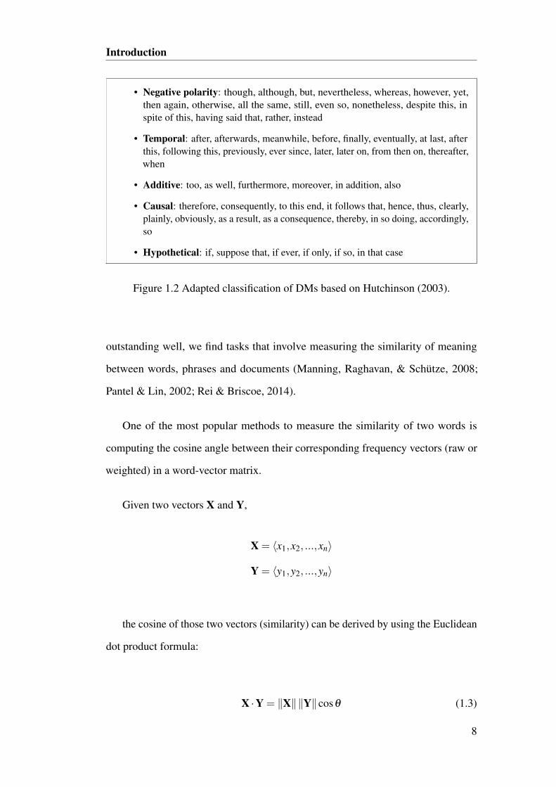
Introduction

• Negative polarity: though, although, but, nevertheless, whereas, however, yet,then again, otherwise, all the same, still, even so, nonetheless, despite this, inspite of this, having said that, rather, instead

• Temporal: after, afterwards, meanwhile, before, finally, eventually, at last, afterthis, following this, previously, ever since, later, later on, from then on, thereafter,when

• Additive: too, as well, furthermore, moreover, in addition, also

• Causal: therefore, consequently, to this end, it follows that, hence, thus, clearly,plainly, obviously, as a result, as a consequence, thereby, in so doing, accordingly,so

• Hypothetical: if, suppose that, if ever, if only, if so, in that case

Figure 1.2 Adapted classification of DMs based on Hutchinson (2003).

outstanding well, we find tasks that involve measuring the similarity of meaning

between words, phrases and documents (Manning, Raghavan, & Schütze, 2008;

Pantel & Lin, 2002; Rei & Briscoe, 2014).

One of the most popular methods to measure the similarity of two words is

computing the cosine angle between their corresponding frequency vectors (raw or

weighted) in a word-vector matrix.

Given two vectors X and Y,

X = ⟨x1,x2, ...,xn⟩

Y = ⟨y1,y2, ...,yn⟩

the cosine of those two vectors (similarity) can be derived by using the Euclidean

dot product formula:

X ·Y = ∥X∥∥Y∥cosθ (1.3)

8

1.3 Motivations

similarity = cos(θ) =X ·Y

∥X∥∥Y∥=

n∑

i=1xi · yi√

n∑

i=1x2

i ·√

n∑

i=1y2

i

(1.4)

Therefore, given the vector space in Fig. 1.3, we can compute the similarity

between the target word and word1, word2 or word3 applying (1.4), being the

maximum degree of similarity when the cosine is 0 (orthogonal vectors, θ is 90

degrees):

Figure 1.3 Vector space adapted fromManning et al. (2008,p.112)

On the basis of the above, at the beginning of this thesis we tested whether some

of the mentioned VSMs in section 1.1 could capture the particular linguistic features

of DMs or not. Using word2vec tool kit trained in a small corpus text8 (17000K

words) provided with the model, we obtained the the cosine distances for the target

word although (the six most similar words are separated by narrower line) shown in

Fig (1.4).

9

Introduction

word Cosine distancethough 0.874836

however 0.829028but 0.776965

because 0.660516nevertheless 0.626817nonetheless 0.589289

have 0.587005still 0.572910yet 0.566393

since 0.535253indeed 0.535020while 0.527823

Table 1.1 Cosine distance obtained with the followingparameters: model, CBOW; size, 200; window, 8.

In sum, it seems that even with such a small corpus as text8, word embeddings

can capture some of the relation signalled by DMs (recall section 1.2), leading us to

further research in this direction as it will be shown in the forthcoming sections.

It remains to be seen why we have chosen word embedding models among others

with similar performance. Although we will not go into mathematical arguments,

Mikolov, Corrado, et al. (2013) have noted that most of the complexity in previous

models (Latent Semantic Analysis (LSA) and Latent Dirichlet Allocation (LDA),

for example) is caused by a non-linear hidden layer, which hinders the possibility

to be trained on large data efficiently. On this basis, Mikolov, Corrado, et al.

(2013) have developed simple models where the non-linear hidden layer is removed,

increasing the speedup and the efficient computation of word similarities, with

similar performance to other state-of-the-art word embedding methods.

• Continuous Bag-of-Words Model (CBOW): "the projection layer is shared for

all words; thus, all words get projected into the same position (their vectors

are averaged)."

• Continuous Skip-gram Model (Skip-gram): "similar to CBOW, but instead

of predicting the current word based on the context, it tries to maximize

classification of a word based on another word in the same sentence".

10

1.4 Research questions

All things considered, henceforth the above models will be used for the proposes

of this thesis.

1.4 Research questions

In the previous sections we have talked about different methods by which we can

represent words with vectors. Likewise, we have introduced a data-driven classifica-

tion of DMs based on Knott (1996) that seems to be followed by our preliminary

small experiment with word embeddings.

Having reached this point and on the basis of previous sections, we are in the

position to address the following research question:

• Despite the fact that DMs signal relations that go beyond simple local phenom-

ena, can word embeddings capture some of these relations and the linguistic

particularities of DMs?

• If so, is it necessary to train a classifier in order to recognise them?

In sum, these are the two main questions that have motivated this thesis and

further research as it will be discussed in next sections.

11

CHAPTER 2

Methods

2.1 Experimental design and set-up

Any experimental design must first have an objective and a clear picture of every

task in order to achieve it. Since the main objective of this master’s thesis is to verify

whether the word embedding can capture the linguistic particularities of DMs or not,

we need a theoretical framework and a classification of DMs based on their context.

That is what we attempted in section 1.2 and 1.3, where adapted classification of

DMs based on Hutchinson (2003) was proposed as a starting point (we reproduced

Fig. 1.2 again for reading facilities).

Note that in this classification some DMs may be ambiguous as to which relation

they signal, but no DM is ambiguous as to which class it belongs in, and that fact

will be of crucial importance for further evaluations.

The second step is to obtain the word representations of the above-mentioned

DMs. For this aim we used word2vec tool kit as detailed subsequently in section 2.2.

On the other hand, the quality of the word representation in vector space depends

to a large extent on the training data, among other parameters. For this reason, we

chose the British National Corpus (BNC), a 100-million-word balanced sample of

13

Methods

• Negative polarity: though, although, but, nevertheless, whereas, however, yet,then again, otherwise, all the same, still, even so, nonetheless, despite this, inspite of this, having said that, rather, instead

• Temporal: after, afterwards, meanwhile, before, finally, eventually, at last, afterthis, following this, previously, ever since, later, later on, from then on, thereafter,when

• Additive: too, as well, furthermore, moreover, in addition, also

• Causal: therefore, consequently, to this end, it follows that, hence, thus, clearly,plainly, obviously, as a result, as a consequence, thereby, in so doing, accordingly,so

• Hypothetical: if, suppose that, if ever, if only, if so, in that case

written (90%) and spoken (10%) English produced in the UK (The British National

Corpus, 2007).

Once the word embeddings are obtained, it remains to be seen how to evaluate

the distances among DMs vectors and if they are grouped accordingly with our

classification in vector space or not. For this task, we will use Weka software (Hall

et al., 2009). Weka is a collection of machine learning algorithms for data mining

tasks, such a classification, regression or clustering. In this thesis, we will focus in

clustering and classification techniques as detailed bellow.

2.2 Procedures used to obtain data and results

In order to obtain the DMs vector representations we needed to preprocess our data

(the British National Corpus, about 100 million tokens). The preprocessing steps

involved tokenisation and lowercasing. The punctuation, however, was not removed

as it is considered a potential feature in our model.

As a result our processed data was formed by 115,376,293 words and a vocabu-

lary size of 158,035.

The models and the parameters introduced in section 1.3 (Skip-gram and CBOW)

were tested with the aim of determining the best configuration for our DMs repre-

14

2.2 Procedures used to obtain data and results

sentation. Therefore, following the comparisons between CBOW and Skip-gram

models made by Mikolov, Chen, et al. (2013) as well as several tests in the vector

spaces provided by Rei and Briscoe (2014)1,2, we set our model with the following

parameters:

• Architecture: skip-gram (skip-gram seems to perform better than CBOW

with infrequent words. Since we assumed DMs to be infrequent words in

comparison with the rest of the vocabulary, skip-gram was used as a main

model).

• The training algorithm: hierarchical softmax (same reason than above: HS

seems to perform better than negative sampling with infrequent words).

• Sub-sampling of frequent words: 10−4 (this parameter indicates that frequent

words, 10−4, are down-sampled, improving the accuracy and speed for large

data sets).

• Dimensionality of the word vectors: 200 (we matched the best results with

values in range 200 to 300).

• Context (window) size: 10.

Before training the model in our data, we converted all the DMs constituted for

more than one word in a single item using underscores (in spite of ⇒ in_spite_of ).

The reason for that has to do with the way word2vec builts its internal vocabulary.

Since we want a single vector for each DMs, underscoring is the most effective

method to achieve so, otherwise, we would obtain an independent vectors for in,

spite and of.

After the training, each word from our data is map onto word-vector, giving as a

result a 200 dimensions vector space containing the target DMs that later on will be1http://www.marekrei.com/projects/vectorsets/2The tests consisted mostly in simple task such as measurements of cos distance or accuracy and

analogy tasks based on \demo-word-accuracy-sh and \demo-analogy.sh scripts included in word2vectool kit.

15

Methods

isolated from the vector space. The resulting subspaces are evaluated by means of

clustering and classification algorithms in Weka software:

The first subspace used for clustering can be encoded in a m− by− n matrix,

where m = 61, n = 202. Each row maps a DM vector (61 DMs) and the columns

(202) are organized respectively as follows: Classes (Temporal, Negative Polarity,

Causal, etc), DM name, features up to 200 (dimensionality of the word vectors).

K-means clustering method is used to partition the 61 observations (DMs vectors)

into 5 clusters (the 5 DMs classes). The results and the evaluation of the clusters are

given in the next chapter.

For classification, we created 10 vector spaces: 5 for training and the other 5 for

the tests. Each training file contains a vector space composed of several DMs of only

one class tagged accordingly, and a random number of DMs from different class

tagged as no. Therefore, we have 5 binary training files for each class of DMs, and 5

test files also binary but containing DMs that have not been seen during training (2

DMs for each of the 5 classes, plus random DMs from different classes).

A Hoeffding decision tree (VFDT) algorithm is used to evaluate the classification.

The results are given below.

16

CHAPTER 3

Results

3.1 Key results obtained in the study

3.1.1 K-means clustering

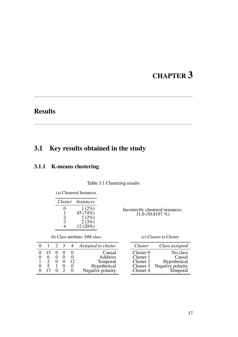
Table 3.1 Clustering results

(a) Clustered Instances

Cluster Instances0 1 (2%)1 45 (74%)2 1 (2%)3 2 (3%)4 12 (20%)

Incorrectly clustered instances:31.0 (50.8197 %)

(b) Class attribute: DM class

0 1 2 3 4 Assigned to cluster0 15 0 0 0 Causal0 6 0 0 0 Additive1 2 0 0 12 Temporal0 5 1 0 0 Hypothetical0 17 0 2 0 Negative polarity

(c) Classes to Cluster

Cluster Class assignedCluster 0 No classCluster 1 CausalCluster 2 HypotheticalCluster 3 Negative polarityCluster 4 Temporal

17

Results

Figure3.1

DM

svs

Class

(cluster0,cluster1,cluster2,cluster3,cluster4)

18

3.1 Key results obtained in the study

Figu

re3.

2C

lust

ers

vsC

lass

(clu

ster

0,cl

uste

r1,c

lust

er2,

clus

ter3

,clu

ster

4)

19

Results

3.1.2 Decision tree classification

Table 3.2 Classification results

Caus. Add. Temp. Hypo. Neg. TOTALCorrect classified 7 (70%) 8 (80%) 10 (10%) 8 (80%) 8 (80%) 41 (82%)Incorrect classified 3 (30%) 2 (20%) 0 (0%) 2 (20%) 2 (20%) 9 (18%)Precision 0.622 0.640 1.000 0.640 0.900 0.760Recall 0.700 0.800 1.000 0.800 0.800 0.820F-Measure 0.659 0.711 1.000 0.711 0.819 0.780

Weighted averages (Precision, Recall and F-Measure )

20

CHAPTER 4

Discussion and Conclusion

4.1 Clustering

From Table 3.1 we can observe that most of DMs (74%) were grouped in the same

cluster, cluster 1. Yet, we expected to find the DMs instances distributed along the

five clusters in line with the five DMs classes.

If we take a closer look at the clustering results, we find that the great majority

of temporal DMs are clustered together in cluster 4 (80%). Looking at the sentences

where those DMs appear in the BNC corpus, we find that temporal DMs are mostly

used along with temporal nouns and adverbs of time such a day, time, shortly, soon,

etc. In the same way, the only temporal DMs that is clustered in cluster 0 has certain

differential particularities: although ever since can appear in different positions in a

sentence, in our corpus it is almost always seen in the final position followed by a

dot, which in our model is taken as a potential feature when word vectors are built.

On the other hand, the negative polarity DMs despite this and in spite of are

clustered in cluster 3. They seem to share the same context schema unfeasible for

most of the other negative polarity DMs: the DM preceded by another DM such a

nevertheless, however, so or the coordinating conjunctions and, or and but.

21

Discussion and Conclusion

Finally, we have the hypothetical DM suppose that clustered in cluster 2. In this

case, it is not clear whether suppose that can be taken as a pure DM or not. Since we

followed Hutchinson (2003) in our initial DMs classification, we decided to include

it for further comparisons with the results obtained by this researcher.

Although DMs are quite diverse from a syntactic point of view, most of them

fall into four syntactic classes: coordinators, subordinators, conjunct adverbs and

prepositional phrases. However, a few of them, such as suppose that, fall into a

different category: phrases which take sentential complements. For that reason, the

schema of the sentence is often different. Likewise, we can see in our corpus suppose

that preceded by subject pronouns, auxiliary verbs such a don’t or the infinitive

marker to. All of them either infeasible or infrequent with the rest of DMs.

Therefore, our experiment reflects the local lexical effect that word embeddings

capture: words combining with same words have similar vector representations. That

is, those words which do not have similar contexts in terms of lexical items, appear to

be less related in the vector space (different vectors), so that the word representations

are not grouped in similar clusters.

Bringing back our first question research (Despite the fact that DMs signal

relations that go beyond simple local phenomena, can word embeddings capture

some of this relations and the linguistic particularities of DMs?), we conclude

that only those DMs where the above-mentioned lexical effect is greater, can be

represented efficiently by word embeddings, as it has been clearly seen with temporal

DMs. Since those DMs appear with similar adverbs of time or temporal nouns

(greater lexical effect), most of the temporal DMs are clustered in the same cluster.

4.2 Supervised classification

The results obtained in the supervised classification appear to be slightly better with

an overall precision, recall and F-measure of 0.760, 0.820 and 0.780, respectively.

22

4.3 Relevance with respect to state of the art

However, it should be noted that although the number of correct and incorrect

classified instances are the same for the additive, hypothetical and negative polarity

classes (8 vs 2), the confusion matrices are different. In the case of the additive

and the hypothetical classes, all of the instances where classified as no, whereas in

the negative polarity class, all NP instances were correctly classified but also two

instances of no were classified as NP.

Therefore, the best performances are found again with temporal DMs followed

by the NP DMs. Additive, hypothetical and causal DMs obtain, respectively, the

worst performances.

Comparing both methods (clustering and supervised classification), we conclude

that the relations among similar DMs can be induced better with the second, a super-

vised classification which has been trained previously. That is, word embeddings

may provide the required information to establish the common features between

DMs given a known sample.

4.3 Relevance with respect to state of the art

In the beginning of the thesis, we saw related research where vector space models

were used to distinguish polysemous from monosemous prepositions in vector space

and to determine salient vector-space features for a classification of preposition senses

(Koper & Schulte im Walde, 2014). Likewise Rei and Briscoe (2014) investigate

how dependency-based vector space models performs in hyponym generation, that

is, returning a list of all possible hyponyms, given only a single word as input.

It is likely due to the fact that vectors space models are quite new in linguistics,

we only found one research focus exclusively in DMs and data obtained from

corpora (Hutchinson, 2003). Although the goal of that research was the automatic

classification of DMs based on co-occurrence, no vector space models are involved

to achieve it.

23

Discussion and Conclusion

In this regard, Hutchinson (2003) research faced similar problems than us with

hypothetical and additive DMs. He obtained the poorest performance with those

classes, which he believe could be improved by means of reducing the noise of

some co-occurrences. That is, in the case of hypothetical DMs, selecting either only

those instances where modality is clearly involved (the presence of will or may) or

selecting the co-occurrences of DMs in specific position (if in a subordinate clause

is known to collocate with then in the main clause).

4.4 Future steps

We believe on the basis of the results shown along this thesis that certain noise

has been originated during the training process as a result of incorrectly taken

occurrences such too in too far or so in I think so, which are clearly not a DMs. The

former, as Hutchinson (2003) pointed out, could be easily addressed using a parsed

version of BNC and considering only DMs attached at either the S or VP nodes. The

second could also be disambiguated using similar strategies. So it remains to be seen

whether a parsed version of the corpora could improve the overall performance of

the model or not.

24

References

Baroni, M. & Lenci, A. (2010). Distributional Memory: A General Framework forCorpus-Based Semantics. Computational Linguistics, 36(4), 673–721.

Bengio, Y., Ducharme, R., Vincent, P., & Janvin, C. (2003). A Neural ProbabilisticLanguage Model. The Journal of Machine Learning Research, 3, 1137–1155.

Bordería, S. P. (2001). Connectives/Discourse markers. An overview. Quaderns deFilologia. Estudis Literaris. 6, 219–143.

Bullinaria, J. A. & Levy, J. P. (2007). Extracting semantic representations from wordco-occurrence statistics: a computational study. Behavior research methods,39(3), 510–526.

Cohen, R., Goldberg, Y., & Elhadad, M. (2012). Domain Adaptation of a DependencyParser with a Class-Class Selectional Preference Model. In Proceedings ofACL 2012 Student Research Workshop (ACL ’12) (pp. 43–48).

Collobert, R. & Weston, J. (2008). A Unified Architecture for Natural LanguageProcessing : Deep Neural Networks with Multitask Learning. Architecture,20(1), 160–167.

Collobert, R., Weston, J., Bottou, L., Karlen, M., Kavukcuoglu, K., & Kuksa, P.(2011). Natural Language Processing (almost) from Scratch. Journal of Ma-chine Learning Research, 12(Aug), 2493–2537.

Deerwester, S., Dumais, S. T., Furnas, G. W., Landauer, T. K., & Harshman, R.(1990). Indexing by latent semantic analysis. Journal of the American Societyfor Information Science, 41(6), 391–407.

Fraser, B. (1999). What are discourse markers? Journal of Pragmatics, 31(November1996), 931–952.

Hall, M., Frank, E., Holmes, G., Pfahringer, B., Reutemann, P., & Witten, I. H. (2009).The WEKA Data Mining Software: An Update. SIGKDD Explorations, 11(1).

Harris, Z. S. (1954). Distributional structure. Word, 10(23), 146–162.

25

References

Hutchinson, B. (2003). Automatic classification of discourse markers on the basis oftheir co-occurrences. In Proceedings of the ESSLLI Workshop The Meaningand Implementation of Discourse Particles (pp. 1–8).

Knott, A. (1996). A Data-Driven Methodology for Motivating a Set of CoherenceRelations (Doctoral dissertation, University of Edinburgh).

Koper, M. & Schulte im Walde, S. (2014). A Rank-based Distance Measure toDetect Polysemy and to Determine Salient Vector-Space Features for GermanPrepositions. In Proceedings of the 9th Edition of the Language, Resourcesand Evaluation Conference (LREC 2014) (pp. 4459–4466).

Levy, O. & Goldberg, Y. (2014). Linguistic Regularities in Sparse and Explicit WordRepresentations. In Proceedings of the 18th Conference on ComputationalNatural Language Learning (CoNLL 2014) (pp. 171–180).

Manning, C. D., Raghavan, P., & Schütze, H. (2008). Introduction to InformationRetrieval.

Mikolov, T., Chen, K., Corrado, G., & Dean, J. (2013). Distributed Representationsof Words and Phrases and their Compositionality. In Advances in NeuralInformation Processing Systems 26 (NIPS) (pp. 1–9).

Mikolov, T., Corrado, G., Chen, K., & Dean, J. (2013). Efficient Estimation ofWord Representations in Vector Space. In Proceedings of the InternationalConference on Learning Representations (ICLR 2013) (pp. 1–12).

Mikolov, T. & Kombrink, S. (2011). Extensions of recurrent neural network lan-guage model. In International Conference on Acoustics, Speech and SignalProcessing (ICASSP), 2011 IEEE (pp. 5528–5531).

Mikolov, T., Yih, W.-t., & Zweig, G. (2013). Linguistic regularities in continuousspace word representations. In Proceedings of the 2013 Conference of theNorth American Chapter of the Association for Computational Linguistics:Human Language Technologies (June, pp. 746–751).

Niwa, Y. & Nitta, Y. (1995). Co-occurrence Vectors from Corpora vs. DistanceVectors from Dictionaries. In Proceedings of the 15th Conference on Compu-tational Linguistics (p. 6). COLING ’94. Stroudsburg, PA, USA: Associationfor Computational Linguistics.

Pantel, P. & Lin, D. (2002). Discovering word senses from text. In Proceedings ofthe eighth ACM SIGKDD International Conference on Knowledge Discoveryand Data Mining (pp. 613–619).

Pennington, J., Socher, R., & Manning, C. D. (2014). GloVe: Global Vectors forWord Representation. In Proceedings of the 2014 Conference on EmpiricalMethods in Natural Language Processing.

26

References

Rei, M. & Briscoe, T. (2014). Looking for Hyponyms in Vector Space. In Proceedingsof the Eighteenth Conference on Computational Natural Language Learning(pp. 68–77).

Ritter, A. & Etzioni, O. (2010). A Latent Dirichlet Allocation method for SelectionalPreferences. In Proceedings of the 48th Annual Meeting of the Association forComputational Linguistics (July, pp. 424–434).

Sanders, T. J. M., Spooren, W. P. M., & Noordman, L. G. M. (1993). Coherence rela-tions in a cognitive theory of discourse representation. Cognitive Linguistics,4(2), 93–134.

Schiffrin, D. (1987). Discourse Markers. Cambridge University Press.

Séaghdha, D. O. (2010). Latent variable models of selectional preference. In Pro-ceedings of the 48th Annual Meeting of the Association for ComputationalLinguistics (July, pp. 435–444).

Socher, R., Pennington, J., Huang, E. H., Ng, A. Y., & Manning, C. D. (2011). Semi-Supervised Recursive Autoencoders for Predicting Sentiment Distributions. InProceedings of the Conference on Empirical Methods in Natural LanguageProcessing (EMNLP 2011) (2, pp. 151–161).

The British National Corpus, v. 3. ( X. E. (2007). Distributed by Oxford UniversityComputing Services on behalf of the BNC Consortium. Retrieved from http://www.natcorp.ox.ac.uk/

Turney, P. D. (2006). Similarity of Semantic Relations. Association for Computa-tional Linguistics, 32(3).

Turney, P. D. & Pantel, P. (2010). From frequency to meaning: Vector space modelsof semantics. Journal of Artificial Intelligence Research, 37, 141–188.

27

Appendix A:

29

Appendix A:

Table of Cue Phrase Definitions

Extracted from Knott (1996, p.201), where A and C are the propositional contents

of the two related text spans SA and SC.

30

Appendix B:

31

Appendix B:

Small portion of the overall Knott’s taxonomy

Extracted from Knott (1996, p.125).

32