report · rose water quality program to iteratively improve field sampling. the 2014 water quality...
TRANSCRIPT

Report
EC-QUA-FT-0001
White Rose
Environmental Effect Monitoring Program
2014
Volume 1 of 2
Canada-Newfoundland and Labrador Offshore Petroleum Board
5th Floor, TD Place
St. John’s, NL
A1C 6H6
Husky Energy
351 Water Street, Suite 107
St. John’s, NL
A1C 1C2
Signature: Hard copy signed Hard Copy signed Hard copy signed
Initial Last Name / Title:
Dr. M. Skinner and & E. Tracy D. Pinsent
Sr. Environmental Advisor
G. Igloliorte
Manager, HSEQ
Prepared By Reviewed By Approved By
Document No.: WR-HSE-RP-4392 Version No.: 2; January 2017
CONFIDENTIALITY NOTE: No part of this document may be reproduced or transmitted in any form or by any means without the written permission of Husky Oil Operations Limited.
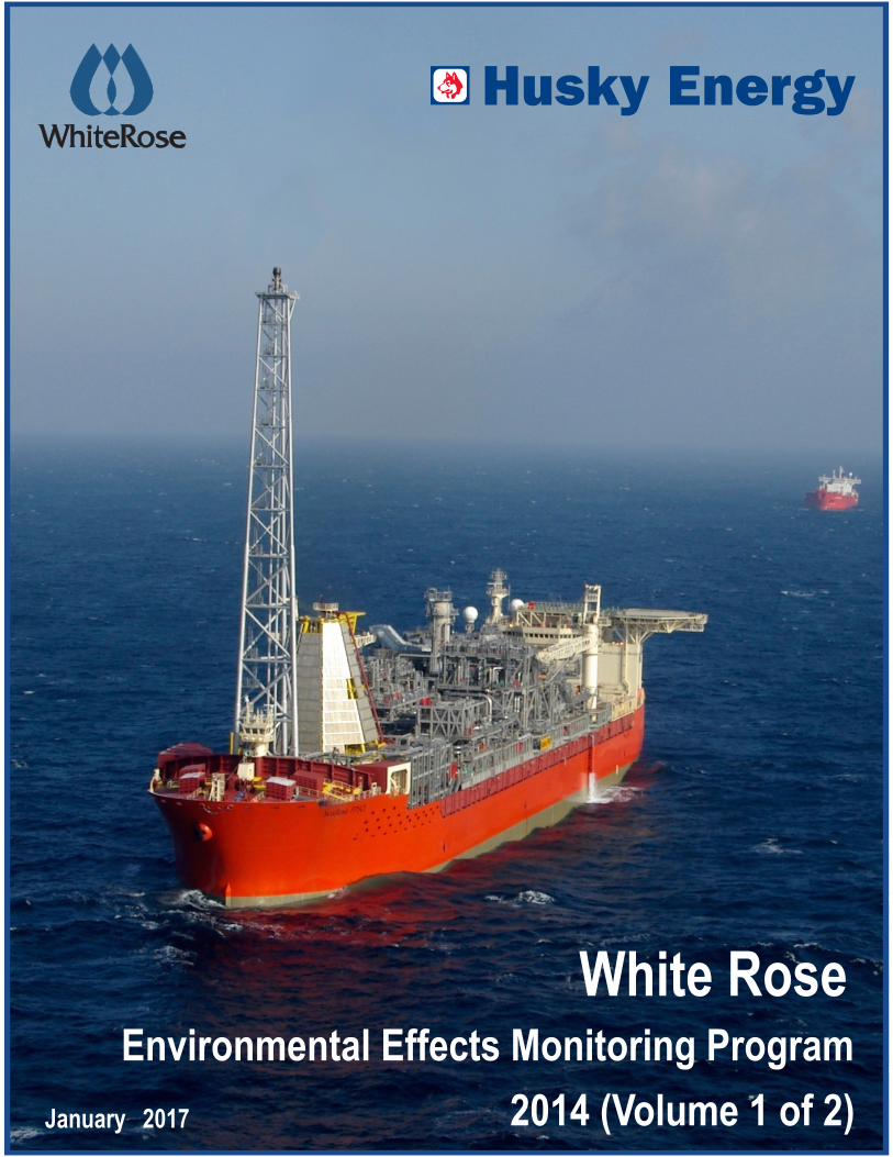
White Rose
2014 (Volume 1 of 2)
Environmental Effects Monitoring Program
January 2017

Submitted To 2014 EEM Program Report
Page i of xv
2014 Executive Summary
The White Rose Environmental Effects Monitoring (EEM) program was designed to evaluate the environmental effects of Husky Energy’s offshore oil drilling and production activities for the White Rose Development. Program design drew on the predictions and information in the White Rose Development Plan Environmental Impact Statement (EIS) and its supporting modelling studies on drill cuttings and produced water dispersion. A baseline study to document pre-development conditions was conducted in 2000 and 2002. This study, combined with stakeholder and regulatory agency consultations, initiated the detailed design phase of the program. Further input on EEM program design was obtained from an expert advisory group called the White Rose Advisory Group. Beyond this, EEM results are reviewed by the regulatory community after each EEM cycle. Comments from the regulatory community on the 2012 EEM program are provided in Appendix A.
The purpose of the EEM program is to assess environmental effects predictions made in the EIS and determine the area demonstrably affected by Husky Energy activities in the White Rose Field. In accordance with the design protocol, the program is updated to accommodate expansions and the establishment of new drill centres within the White Rose Field. The main components of the EEM program are sediment quality, commercial fish and water quality.
Seabed sediments and commercial fish species from the White Rose Field have been collected in 2004, 2005, 2006, 2008, 2010, 2012 and 2014 to assess environmental effects. Sediment samples collected as part of the Sediment Quality Component of the EEM program have been processed for physical and chemical characteristics, toxicity and an evaluation of benthic (seafloor) invertebrate communities. These three sets of measurements are known as the Sediment Quality Triad and are used in a weigh-of-evidence approach to assess changes in overall sediment quality over time and space. For the Commercial Fish Component of the EEM program, American plaice (a common flatfish species) and snow crab (an important commercial shellfish species), have been processed for contaminants (chemical body burden), taint and, for plaice, various health indices. A series of measurements (e.g., length, weight, maturity) are also made on each species.
Seawater samples have been collected at White Rose in 2008, 2010, 2012 and 2014 and processed for chemistry and total suspended solids. The Water Quality sampling program in 2008 was preliminary, with fewer stations and variables sampled in that year than in 2010, 2012 and 2014. In addition to collection of seawater samples, the Water Quality Component of the EEM program in 2010 included sampling for sediment chemistry at Water Quality stations and a produced water modelling component to assess which constituent of produced water (the main liquid discharge from White Rose) would have a higher probability of being detected in seawater samples. The 2012 Water Quality program included seawater sampling, sediment chemistry sampling at Water Quality stations and a modelling component to assess potential concentrations of produced water constituents in sediments. Modelling was used as part of the White Rose Water Quality program to iteratively improve field sampling. The 2014 Water Quality program included seawater sampling and sediment chemistry sampling at Water Quality stations; there was no modelling component in the 2014 Water Quality program.
Figure 1 illustrates the components of the EEM program.

Submitted To 2014 EEM Program Report
Page ii of xv
Figure 1 EEM Program Components
Notes: BTEX: Benzene, toluene, ethylbenzene, xylene. PAH: Polycyclic aromatic hydrocarbon.
TSS: Total suspended solids.
This report provides the results from the seventh round of post-development sampling under the program conducted in the summer (commercial fish survey) and fall (sediment and water survey) of 2014. The findings are interpreted in the context of results of previous sampling years and the baseline data collected pre-development.
Sediment Quality
In 2014, seafloor sediments were sampled for Sediment Quality Triad variables at 53 locations surrounding the Northern, Central, Southern, North Amethyst and South White Rose Extension Drill Centres. This allowed an assessment of environmental conditions over an area of 1,200 km² around the White Rose Field.
Analysis of sediment physical and chemical characteristics showed that concentrations of drill mud hydrocarbons and barium were elevated near active drill centres and concentrations decreased with distance from drill centres, as expected. To a lesser extent, sediment lead, fines, TOC, ammonia, sulphide, sulphur, and redox potential were also affected by drilling. There was no evidence of project effects on other physical and chemical parameters measured in sediments.
Maximum drill mud hydrocarbon (hydrocarbons in the >C10-C21 range) and barium concentrations at White Rose in 2014 were 120 mg/kg and 1,400 mg/kg, respectively. The estimated distance over which hydrocarbons concentrations were correlated with distance from active drill centres (i.e., the threshold distance) extended to an average 5.8 km in 2014, which was greater than upper 95% confidence intervals noted for both 2010 and 2012, but the mean is less than in previous years. The distance over which

Submitted To 2014 EEM Program Report
Page iii of xv
barium concentrations were correlated with distance from active drill centres extended to an average of 1 km, unchanged from 2012 and less than in previous years.
In 2014, project effects on sediment lead concentrations were noted, but threshold distances for lead have consistently decreased from a maximum 1.5 km in 2006 to a minimum 0.6 km in 2014; unchanged from 2012. For the first time, project effects on sediment fines concentrations were noted in 2014, with an estimated threshold distance of 0.7 km from the nearest active drill centre. Similarly, project effects on both TOC and ammonia were observed for the first time in 2014 sampling. The absolute magnitude of TOC values across all stations, including reference stations in 2014, was greater than those observed in previous years. For ammonia, all recorded 2014 concentrations were below the 12.2 mg/kg background threshold.
Project effects were also established for sulphide, sulphur and redox potential. No threshold distance could be reliably estimated for each of these analytes; however, values varied significantly with distance from the nearest active drill centre. For redox potential, the only value below baseline concentrations (found near the Southern Drill Centre) was well within the range of oxic conditions. Sulphur levels increased modestly at some stations less than 1 km from active drill centres, with levels ranging from approximately 0.02% to 0.18% in the immediate vicinity of drill centres.
Sediments from certain stations were found to cause toxicity in the laboratory in 2014, though toxicity outcomes could not be related to project effects on sediment physical and chemical characteristics. Of 53 sediment samples tested for toxicity, two significantly reduced survival of amphipods in the laboratory and three significantly reduced bacterial luminescence in 2014. Percent amphipod survival in 2014 was not significantly correlated with any assessed variables. Further, no samples resulted in significant toxicity in both laboratory tests.
There continues to be no detectable project effects on benthic invertebrate community richness1. As has been noted since 2008, evidence of effects on total abundance was marginal and benthic biomass was affected by project activity. Declines in echinoderm biomass at drill centre locations relative to reference sites appear to be driving this total biomass decline. There was also evidence of effects on one species of polychaete (Paraonidae: a marine worm). There was little evidence of project effects on Spionidae (a polychaete), Tellinidae (a bivalve) and amphipods (a crustacean) in 2014. Total abundance, biomass and the abundance of Paraonidae were lower in sediments with high concentrations of barium and >C10-C21 hydrocarbons near active drill centres.
Overall, some sediment chemical characteristics and indices of benthic community at White Rose were affected by project activity, based on a weight of evidence approach.
Commercial Fish
During the summer of 2014, samples of American plaice and snow crab were collected near White Rose (the Study Area) and at four Reference Areas, located approximately 28 km to the southwest, northwest, southeast and northeast of White Rose. As noted above, samples were analyzed for chemical body burden and taint. In addition, analyses were also performed on American plaice for a variety of fish health indices, as outlined in
1 Number of taxonomic groups per unit area.

Submitted To 2014 EEM Program Report
Page iv of xv
Figure 1. Physical measurements taken on American plaice and snow crab (e.g., length, weight, maturity) were used as supporting information for analyses of body burden, taint and health.
In 2014, metal and hydrocarbon concentrations in American plaice and snow crab tissue continued to show that body burden in these species is mostly unaffected by project activities. For plaice liver, percent fat and concentrations of >C21-C32 hydrocarbons were significantly lower in the Study Area and percent moisture and concentrations of cadmium and zinc were significantly higher in the Study Area. For crab tissue, significant differences in trends between the Study and Reference Areas were noted for silver and mercury. Mercury concentrations remained relatively constant in the Study Area, while Reference Areas concentrations declined steeply from elevated levels in 2005. Silver has shown significant trends (initial values decreasing followed by an increase) at both the Study Area and Reference Areas; however, Study Area concentrations of silver have generally remained within the range of variability of Reference Area concentrations.
The results of taste tests, carried out at the Marine Institute, demonstrated that the two species were not tainted. Indicators of fish health used to evaluate potential effects, or precursors of effects, on America plaice showed that the general health and condition of this species was similar in the Study and Reference Areas.
Overall, analyses of fish tissue chemistry, taste and fish health characteristics revealed no compelling evidence of effects of project activities on commercial fish.
Water Quality
In the fall of 2014, water samples were collected in the vicinity of the SeaRose floating, production, storage and offloading (FPSO) vessel and in two Reference Areas, located approximately 28 km to the northeast and northwest. Samples were processed for parameters listed in Figure 1. Results indicated no difference in water chemistry between the Study and Reference Areas in 2014, other than higher barium concentrations at mid-depth in Reference Area samples and at the surface in near-field Study Area samples near the SeaRose FPSO. Differences were small. Examination of 2010, 2012 and 2014 data indicated that barium concentrations have generally varied from approximately 3 to 9 µg/L, with levels in all Areas lower than the background average for oceanic regions. Although barium is a constituent of drill muds, some natural barium in seawater samples is to be expected.
Conclusions
The following sediment quality variables were affected by the White Rose development in 2014: drill mud hydrocarbons, barium, fines, lead, TOC, ammonia, sulphide, sulphur redox, total benthic invertebrate abundance and biomass. Of the benthic invertebrate taxa examined, one family of polychaete worms (Paraonidae) was most affected by drilling discharge. Despite changes in sediment contamination and benthic invertebrate responses since drilling began at White Rose in 2004, there has not been any consistent accentuation of contamination or responses in sediment toxicity or benthic community structure over those years. As there has been no continued degradation at White Rose, sediment contamination and the benthic invertebrate responses justify continued monitoring, without further mitigation.

Submitted To 2014 EEM Program Report
Page v of xv
Sediment contamination and effects on benthos noted in 2014 and in previous years have not translated into effects on the fisheries resources, as indicated by fish health assessment and taint tests. No project-related tissue contamination was noted for crab and plaice. Neither species were tainted; plaice health was similar between White Rose and more distant Reference Areas. These results indicate that changes in sediments and benthic community have not affected fish in EEM years (i.e., since baseline collections in 2000 and 2002).
There was no evidence of project effects on water quality.

Submitted To 2014 EEM Program Report
Page vi of xv
Acknowledgements
Project management for the White Rose EEM program was executed by Ellen Tracy at Stantec Consulting Ltd. (St. John’s, Newfoundland and Labrador). Participants in the commercial fish survey included Doug Rimmer and Melinda Watts from Stantec Consulting Ltd., and Adam Templeton and Joseph Woodford from Oceans Ltd. (St. John’s, Newfoundland and Labrador). Participants in the sediment and water survey included Doug Rimmer, Scott Finlay, Kristian Greenham, Alexandra Eaves, Justin Bath and Jim Harrison from Stantec Consulting Ltd. Fugro Jacques Geosurveys Inc. (Rob Boland and Shane Sullivan) provided geopositional services for sediment and water collections. Benthic invertebrate sorting, identification and enumeration was led by Patricia Pocklington of Arenicola Marine (Wolfville, Nova Scotia). Chemical analyses of tissues and sediment toxicity tests were conducted by petroforma inc. (St. John's, Newfoundland and Labrador). Chemical analyses of sediment were conducted by petroforma inc. and Maxxam Analytics (Halifax, Nova Scotia). Chemical analyses of water were conducted by Maxxam Analytics and RPC (Fredericton, New Brunswick). Particle size analysis was conducted by Maxxam Analytics. Fish and shellfish taste tests were performed at the Marine Institute of Memorial University. Laboratory analyses for fish health indicators were supervised by Dr. Juan Perez Casanova of Oceans Ltd. Sediment quality, body burden and fish health data were analyzed by Dr. Marc Skinner (Stantec Consulting Ltd.). Water quality data analysis was performed by Dr. Elisabeth DeBlois (Elisabeth DeBlois Inc., St. John’s, Newfoundland and Labrador) and Dr. Marc Skinner. Drs Elisabeth DeBlois, Marc Skinner and Juan Perez Casanova wrote sections of the report. Editing and report consolidation was performed by Ellen Tracy (Stantec Consulting Ltd.). Lois Strangemore and Ryan Melanson (Stantec Consulting Ltd.) provided administrative and graphics support, respectively. Ellen Tracy and Mary Murdoch reviewed the report from a quality control perspective at Stantec Consulting Ltd. The report was prepared and finalized under the direction of David Pinsent (Husky Energy). David Pinsent (Husky Energy) reviewed the document before final production.

Submitted To 2014 EEM Program Report
Page vii of xv
TABLE OF CONTENTS
Page No.
1.0 INTRODUCTION .............................................................................................................. 1
1.1 Project Setting and Field Layout ............................................................................ 1
1.2 Project Commitments .............................................................................................. 2
1.3 EEM Program Design .............................................................................................. 2
1.4 EEM Program Objectives ........................................................................................ 2
1.5 White Rose EIS Predictions .................................................................................... 3
1.6 EEM Program Components and Monitoring Variables.......................................... 4
1.7 Monitoring Hypotheses ........................................................................................... 5
1.8 EEM Sampling Design ............................................................................................. 6
1.8.1 Modifications to the Sediment Component ................................................................. 6
1.8.2 Modifications to the Commercial Fish Component .................................................. 17
1.8.3 Modifications to the Water Quality Component ........................................................ 25
2.0 SCOPE ............................................................................................................................31
2.1 Background Material ..............................................................................................31
3.0 ABBREVIATIONS, ACRONYMS AND UNITS OF MEASURE ........................................33
4.0 PROJECT ACTIVITIES ...................................................................................................35
4.1 Introduction .............................................................................................................35
4.2 Project Activities .....................................................................................................35
4.3 Drilling and Completions Operations ....................................................................36
4.3.1 Drilling Mud and Completion Fluids Discharges ...................................................... 36
4.3.2 Other Discharges from Drilling Operations ............................................................... 41
4.4 SeaRose FPSO Production Operations .................................................................41
4.5 Supply Vessel Operations ......................................................................................42
5.0 SEDIMENT COMPONENT ..............................................................................................43
5.1 Methods ...................................................................................................................43
5.1.1 Field Collection ............................................................................................................. 43
5.1.2 Laboratory Analysis ..................................................................................................... 46
5.1.3 Data Quality Control ..................................................................................................... 54
5.1.4 Data Analysis ................................................................................................................ 54
5.2 Results .....................................................................................................................57
5.2.1 Physical and Chemical Characteristics ..................................................................... 57
5.2.2 Toxicity ........................................................................................................................ 105
5.2.3 Benthic Community Structure .................................................................................. 106

Submitted To 2014 EEM Program Report
Page viii of xv
5.3 Summary of Results ............................................................................................. 139
5.3.1 Whole-Field Response ............................................................................................... 139
5.3.2 Effects of Individual Drill Centres ............................................................................. 141
6.0 COMMERCIAL FISH COMPONENT ............................................................................. 143
6.1 Methods ................................................................................................................. 143
6.1.1 Field Collection ........................................................................................................... 143
6.1.2 Laboratory Analysis ................................................................................................... 145
6.1.3 Data Analysis .............................................................................................................. 152
6.2 Results ................................................................................................................... 155
6.2.1 Biological Characteristics ......................................................................................... 155
6.2.2 Body Burden ............................................................................................................... 161
6.2.3 Taste Tests .................................................................................................................. 173
6.2.4 Fish Health .................................................................................................................. 176
6.3 Summary of Results ............................................................................................. 181
6.3.1 Biological Characteristics ......................................................................................... 181
6.3.2 Body Burden ............................................................................................................... 182
6.3.3 Taste Tests .................................................................................................................. 182
6.3.4 Fish Health Indicators ................................................................................................ 183
7.0 WATER QUALITY COMPONENT ................................................................................. 184
7.1 Background ........................................................................................................... 184
7.2 Seawater ................................................................................................................ 184
7.2.1 Modelling Study .......................................................................................................... 184
7.2.2 Field Sampling ............................................................................................................ 185
7.3 Sediment ............................................................................................................... 197
7.3.1 Modelling Study .......................................................................................................... 197
7.3.2 Field Sampling ............................................................................................................ 197
7.4 Summary of Results ............................................................................................. 207
7.4.1 Water ............................................................................................................................ 207
7.4.2 Sediment ..................................................................................................................... 208
8.0 DISCUSSION ................................................................................................................ 209
8.1 Sediment Quality Component .............................................................................. 209
8.1.1 Physical and Chemical Characteristics ................................................................... 209
8.1.2 Laboratory Toxicity Tests .......................................................................................... 213
8.1.3 Benthic Invertebrate Community Structure ............................................................. 214
8.1.4 Sediment Quality Summary ....................................................................................... 215
8.2 Commercial Fish Component .............................................................................. 216
Submitted To 2014 EEM Program Report
Page ix of xv
8.2.1 Body Burden ............................................................................................................... 216
8.2.2 Taste Tests .................................................................................................................. 217
8.2.3 Fish Health Indicators ................................................................................................ 218
8.2.4 Commercial Fish Summary ....................................................................................... 220
8.3 Water Quality Component .................................................................................... 220
8.3.1 Seawater Chemistry ................................................................................................... 221
8.3.2 Sediment Iron Concentration .................................................................................... 222
8.3.3 Water Quality Summary ............................................................................................. 222
8.4 Summary of Effects and Monitoring Hypotheses ............................................... 222
8.5 Recommendations for the 2014 EEM program ................................................... 225
8.5.1 Sediment Quality ........................................................................................................ 225
8.5.2 Commercial Fish......................................................................................................... 225
8.5.3 Water Quality .............................................................................................................. 226
8.6 Regulator Comments on the 2012 EEM Program ............................................... 226
9.0 REFERENCES .............................................................................................................. 227
9.1 Personal Communications ................................................................................... 227
9.2 Literature Cited ..................................................................................................... 227
LIST OF FIGURES
Page No.
Figure 1-1 Location of the White Rose Oilfield ..................................................................................... 1 Figure 1-2 White Rose Oilfield Layout .................................................................................................. 1 Figure 1-3 EEM Program Components ................................................................................................ 5 Figure 1-4 2000 Baseline Program Sediment Quality Stations ............................................................ 7 Figure 1-5 2004 EEM Program Sediment Quality Stations .................................................................. 8 Figure 1-6 2005 EEM Program Sediment Quality Stations .................................................................. 9 Figure 1-7 2006 EEM Program Sediment Quality Stations ................................................................ 10 Figure 1-8 2008 EEM Program Sediment Quality Stations ................................................................ 11 Figure 1-9 2010 EEM Program Sediment Quality Stations ................................................................ 12 Figure 1-10 2012 EEM Program Sediment Quality Stations ................................................................ 13 Figure 1-11 2014 EEM Program Sediment Quality Stations ................................................................ 14 Figure 1-12 2004 EEM Program Commercial Fish Transect Locations ............................................... 18 Figure 1-13 2005 EEM Program Commercial Fish Transect Locations ............................................... 19 Figure 1-14 2006 EEM Program Commercial Fish Transect Locations ............................................... 20 Figure 1-15 2008 EEM Program Commercial Fish Transect Locations ............................................... 21 Figure 1-16 2010 EEM Program Commercial Fish Transect Locations ............................................... 22 Figure 1-17 2012 EEM Program Commercial Fish Transect Locations ............................................... 23 Figure 1-18 2014 EEM Program Commercial Fish Transect Locations ............................................... 24 Figure 1-19 2000 Baseline Program Water Quality Stations ............................................................... 26 Figure 1-20 2008 EEM Program Water Quality Stations ..................................................................... 27 Figure 1-21 2010 EEM Program Water Quality Stations ..................................................................... 28 Figure 1-22 2012 EEM Program Water Quality Stations ..................................................................... 29 Figure 1-23 2014 EEM Program Water Quality Stations ..................................................................... 30

Submitted To 2014 EEM Program Report
Page x of xv
Figure 5-1 2014 Sediment Quality Triad Stations .............................................................................. 44 Figure 5-2 Sediment Corer Diagram .................................................................................................. 45 Figure 5-3 Sediment Corer ................................................................................................................. 45 Figure 5-4 Gas Chromatogram Trace for PureDrill IA35-LV .............................................................. 50 Figure 5-5 Amphipod Survival Test .................................................................................................... 51 Figure 5-6 Spearman Rank Correlations with Distance from the Nearest Active Drill Centre for
>C10-C21 Hydrocarbons ..................................................................................................... 59 Figure 5-7 Variations in >C10-C21 Concentrations with Distance from the Nearest Active Drill
Centre (all Years) .............................................................................................................. 60 Figure 5-8 Location of Stations with >C10-C21 Hydrocarbon Values within the Baseline Range
(not detected), Stations Showing Mild Enrichment up to 5 mg/kg, and Stations with
Values Greater than 5 mg/kg (2014) ................................................................................. 61 Figure 5-9 Dot Density Plot of >C10-C21 Hydrocarbon Values by Year .............................................. 62 Figure 5-10 Spearman Rank Correlations with Distance from the Nearest Active Drill Centre for
Barium ............................................................................................................................... 63 Figure 5-11 Variations in Barium Concentrations with Distance from the Nearest Active Drill
Centre (all Years) .............................................................................................................. 64 Figure 5-12 Location of Stations with Barium Levels Within the Baseline Range, Stations
Showing Mild Enrichment up to 300 mg/kg, and Stations with Values Greater than
300 mg/kg (2014) .............................................................................................................. 65 Figure 5-13 Dot Density Plot of Barium Values by Year ...................................................................... 66 Figure 5-14 Spearman Rank Correlations with Distance from the Nearest Active Drill Centre for
Fines ................................................................................................................................. 67 Figure 5-15 Variations in Percent Fines with Distance from the Nearest Active Drill Centre (all
Years) ................................................................................................................................ 68 Figure 5-16 Location of Stations with Percent Fines Levels (2014) Within and Above the
Baseline Range ................................................................................................................. 69 Figure 5-17 Dot Density Plot of Percent Fines by Year........................................................................ 70 Figure 5-18 Spearman Rank Correlations with Distance from the Nearest Active Drill Centre for
Gravel ................................................................................................................................ 71 Figure 5-19 Variations in Percent Gravel with Distance from the Nearest Active Drill Centre (all
Years) ................................................................................................................................ 72 Figure 5-20 Dot Density Plot of Percent Gravel by Year ...................................................................... 73 Figure 5-21 Spearman Rank Correlations with Distance from the Nearest Active Drill Centre for
Total Organic Carbon ........................................................................................................ 74 Figure 5-22 Variations in Total Organic Carbon with Distance from the Nearest Active Drill
Centre (all Years) .............................................................................................................. 75 Figure 5-23 Location of Stations with Total Organic Carbon Levels (2014) Within and Above the
Baseline Range ................................................................................................................. 76 Figure 5-24 Dot Density Plot of Total Organic Carbon by Year ........................................................... 77 Figure 5-25 Spearman Rank Correlations with Distance from the Nearest Active Drill Centre for
Ammonia ........................................................................................................................... 79 Figure 5-26 Variations in Ammonia Concentrations with Distance from the Nearest Active Drill
Centre (all Years) .............................................................................................................. 80 Figure 5-27 Location of Stations with Ammonia Concentrations (2014) Within and Above the
Background Range ........................................................................................................... 81 Figure 5-28 Dot Density Plot of Ammonia Concentrations by Year ..................................................... 82 Figure 5-29 Spearman Rank Correlations with Distance from the Nearest Active Drill Centre for
Sulphide ............................................................................................................................ 83 Figure 5-30 Variations in Sulphide with Distance from the Nearest Active Drill Centre (all Years) ..... 84 Figure 5-31 Location of Stations with Sulphide (2014) Within and Above the Baseline Range .......... 85
Submitted To 2014 EEM Program Report
Page xi of xv
Figure 5-32 Dot Density Plot of Sulphide Concentrations by Year ...................................................... 86 Figure 5-33 Spearman Rank Correlations with Distance from the Nearest Active Drill Centre for
Sulphur .............................................................................................................................. 87 Figure 5-34 Variations in Sulphur Concentrations with Distance from the Nearest Active Drill
Centre (all Years) .............................................................................................................. 88 Figure 5-35 Location of Stations with Sulphur (2014) Within and Above the Background Range ....... 89 Figure 5-36 Dot Density Plot of Sulphur Concentrations by Year ........................................................ 90 Figure 5-37 Spearman Rank Correlations with Distance from the Nearest Active Drill Centre for
Metals PC1 ........................................................................................................................ 91 Figure 5-38 Variations in Metals PC1 Scores with Distance from the Nearest Active Drill Centre
(all Years) .......................................................................................................................... 92 Figure 5-39 Dot Density Plot of Metals PC1 Scores by Year ............................................................... 93 Figure 5-40 Spearman Rank Correlations with Distance from the Nearest Active Drill Centre for
Lead .................................................................................................................................. 94 Figure 5-41 Variations in Lead with Distance from the Nearest Active Drill Centre (all Years) ........... 95 Figure 5-42 Location of Stations with Lead (2014) Within and Above the Baseline Range ................ 96 Figure 5-43 Dot Density Plot of Lead by Year ...................................................................................... 97 Figure 5-44 Spearman Rank Correlations with Distance from the Nearest Active Drill Centre for
Strontium ........................................................................................................................... 98 Figure 5-45 Variations in Strontium with Distance from the Nearest Active Drill Centre (all Years) .... 99 Figure 5-46 Dot Density Plot of Strontium by Year ............................................................................ 100 Figure 5-47 Spearman Rank Correlations with Distance from the Nearest Active Drill Centre for
Redox Potential ............................................................................................................... 101 Figure 5-48 Variations in Redox Potential with Distance from the Nearest Active Drill Centre (all
Years) .............................................................................................................................. 102 Figure 5-49 Location of Stations with Redox Potential (2014) Within and Above the Baseline
Range .............................................................................................................................. 103 Figure 5-50 Dot Density Plot of Redox Potential by Year .................................................................. 104 Figure 5-51 Dot Density Plot of Laboratory Amphipod Survival by Year ........................................... 106 Figure 5-52 Spearman Rank Correlations with Distance from the Nearest Active Drill Centre for
Total Benthic Abundance ................................................................................................ 109 Figure 5-53 Variation in Total Abundance (#/m²) with Distance from Nearest Active Drill Centre
(all Years) ........................................................................................................................ 110 Figure 5-54 Location of Stations with Total Abundance Values Within and Below the Baseline
Range (2014) .................................................................................................................. 111 Figure 5-55 Dot Density Plot of Total Benthic Abundance by Year ................................................... 112 Figure 5-56 Spearman Rank Correlations with Distance from the Nearest Active Drill Centre for
Total Benthic Biomass .................................................................................................... 113 Figure 5-57 Variation in Total Benthic Biomass (g/m²) with Distance From Nearest Active Drill
Centre (all Years) ............................................................................................................ 114 Figure 5-58 Location of Stations with Total Biomass Values Within and Below the Baseline
Range (2014) .................................................................................................................. 115 Figure 5-59 Variation in Echinoderm Abundance (#/m²) with Distance From Nearest Active Drill
Centre (all Years) ............................................................................................................ 117 Figure 5-60 Location of Stations with Echinoderm Abundance (#/m²) Within and Below the
Baseline Range (2014) ................................................................................................... 118 Figure 5-61 Dot Density Plot of Total Benthic Biomass by Year ........................................................ 119 Figure 5-62 Spearman Rank Correlations with Distance from the Nearest Active Drill Centre for
Taxa Richness ................................................................................................................ 120 Figure 5-63 Variation in Taxa Richness with Distance From Nearest Active Drill Centre
(all Years) ........................................................................................................................ 121

Submitted To 2014 EEM Program Report
Page xii of xv
Figure 5-64 Location of Stations with Richness Values Within and Below the Baseline Range
(2014) .............................................................................................................................. 122 Figure 5-65 Dot Density Plot of Taxa Richness by Year .................................................................... 123 Figure 5-66 Spearman Rank Correlations with Distance from the Nearest Active Drill Centre for
Paraonidae Abundances ................................................................................................. 124 Figure 5-67 Variation in Paraonidae Abundance (#/m²) with Distance from Nearest Active Drill
Centre (all Years) ............................................................................................................ 125 Figure 5-68 Location of Stations with Paraonidae Abundance Values Within and Below the
Baseline Range (2014) ................................................................................................... 127 Figure 5-69 Dot Density Plot of Paraonidae Abundance by Year ...................................................... 128 Figure 5-70 Spearman Rank Correlations with Distance from the Nearest Active Drill Centre for
Spionidae Abundances ................................................................................................... 129 Figure 5-71 Variation in Spionidae Abundance (#/m²) with Distance From Nearest Active Drill
Centre (all Years) ............................................................................................................ 130 Figure 5-72 Dot Density Plot of Spionidae Abundance by Year ........................................................ 131 Figure 5-73 Spearman Rank Correlations with Distance from the Nearest Active Drill Centre for
Tellinidae Abundance...................................................................................................... 132 Figure 5-74 Variation in Tellinidae Abundance (#/m²) with Distance From Nearest Active Drill
Centre (all Years) ............................................................................................................ 133 Figure 5-75 Location of Stations with Tellinidae Abundance Values Within and Below the
Baseline Range (2014) ................................................................................................... 134 Figure 5-76 Dot Density Plot of Tellinidae Abundance by Year ......................................................... 135 Figure 5-77 Spearman Rank Correlations with Distance from the Nearest Active Drill Centre for
Amphipoda Abundance ................................................................................................... 136 Figure 5-78 Variation in Amphipoda Abundance (#/m²) with Distance From Nearest Active Drill
Centre (all Years) ............................................................................................................ 137 Figure 5-79 Dot Density Plot of Amphipoda Abundance by Year ...................................................... 138 Figure 6-1 2014 EEM Program Transect Locations ......................................................................... 144 Figure 6-2 Plaice Taste Test Preparations ....................................................................................... 149 Figure 6-3 Questionnaire for Taste Evaluation by Triangle Test ...................................................... 150 Figure 6-4 Questionnaire for Taste Evaluation by Hedonic Scaling ................................................. 151 Figure 6-5 Box Plot of Plaice Gutted Weight (g) .............................................................................. 156 Figure 6-6 Box Plots of Variable Concentrations in Plaice Livers in Reference and Study Areas
(2014) .............................................................................................................................. 162 Figure 6-7 Variations in Area Means of Detectable Metals and Hydrocarbons in Plaice Liver
Composites from 2004 and 2014 .................................................................................... 164 Figure 6-8 Box Plots of Variable Concentrations in Plaice Fillets in Reference and Study Areas
(2014) .............................................................................................................................. 166 Figure 6-9 Variations in Fat, Moisture, Mercury, Arsenic and Zinc Concentrations in Plaice
Fillets from 2004 to 2014 ................................................................................................ 168 Figure 6-10 Box Plots of Variable Concentrations in Crab Claw in Reference and Study Areas
(2014) .............................................................................................................................. 170 Figure 6-11 Variation in Area Means of Detectable Variable Concentrations in Crab Claw
Composites from 2004 to 2014 ....................................................................................... 172 Figure 6-12 Plaice Frequency Histogram for Hedonic Scaling Taste Evaluation (2014) ................... 173 Figure 6-13 Crab Frequency Histogram for Hedonic Scaling Taste Evaluation (2014) ..................... 175 Figure 6-14 Box Plots of EROD Activity in the Liver of: Top) Pre-spawning (F-510 to F-540); and
Bottom) Spent (F-550 to F-580) Female Plaice .............................................................. 177 Figure 7-1 Water Quality Stations 2014 ........................................................................................... 186 Figure 7-2 Niskin Bottle Water Samples .......................................................................................... 187 Figure 7-3 Boxplots of Water Chemistry by Area and Depth for 2014 ............................................. 192
Submitted To 2014 EEM Program Report
Page xiii of xv
Figure 7-4 Barium Concentration in the Combined Study and Reference Areas in 2010 2012
and 2014 ......................................................................................................................... 196 Figure 7-5 Spearman Rank Correlations with Distance from SeaRose FPSO for Iron
Concentrations in Sediments .......................................................................................... 200 Figure 7-6 Spearman Rank Correlations with Distance from the SeaRose FPSO for Iron
Residuals ........................................................................................................................ 200 Figure 7-7 Variation in Iron Concentrations in Sediments (mg/kg) with Distance from the
SeaRose FPSO (all Years) ............................................................................................. 202 Figure 7-8 Variation in Iron Residuals with Distance from the SeaRose FPSO (all Years) ............. 203 Figure 7-9 Location of Stations with Iron Concentrations Within and Outside the Baseline
Range (2014) .................................................................................................................. 204 Figure 7-10 Location of Stations with Iron Residuals Within and Outside the Baseline Range
(2014) .............................................................................................................................. 205 Figure 7-11 Dot Density Plot of Iron Concentrations in Sediments (mg/kg) by Year ......................... 206 Figure 7-12 Dot Density Plot of Iron Residuals by Year ..................................................................... 207
LIST OF TABLES
Page No.
Table 1-1 Table of Concordance between Baseline and 2014 EEM Sediment Stations .................. 16 Table 4-1 Cuttings and Water-based Mud Discharges from 2003 to December 2014 ..................... 37 Table 4-2 Cuttings and Synthetic-based Mud Discharges from 2003 to December 2014 ................ 38 Table 4-3 Completion Fluid Discharges from 2003 to December 2014 ............................................ 39 Table 5-1 Date of Sediment Field Programs ..................................................................................... 43 Table 5-2 Particle Size Classification ................................................................................................ 47 Table 5-3 Sediment Chemistry Variables (2000, 2004, 2005, 2006, 2008, 2010, 2012 and
2014) ................................................................................................................................. 48 Table 5-4 Summary of Commonly Detected Sediment Variables (2014) ......................................... 58 Table 5-5 Results of Threshold Regressions on Distance from the Nearest Active Drill Centre
for >C10-C21 Hydrocarbons ................................................................................................ 59 Table 5-6 Repeated-measures Regression Testing for Changes in >C10-C21 Concentrations
over Time .......................................................................................................................... 62 Table 5-7 Results of Threshold Regressions on Distance from the Nearest Active Drill Centre
for Barium .......................................................................................................................... 63 Table 5-8 Repeated-measures Regression Testing for Changes in Barium Concentrations over
Time .................................................................................................................................. 66 Table 5-9 Repeated-measures Regression Testing for Changes in Percent Fines over Time ........ 70 Table 5-10 Repeated-measures Regression Testing for Changes in Percent Gravel over Time ...... 73 Table 5-11 Repeated-measures Regression Testing for Changes in Percent Total Organic
Carbon over Time ............................................................................................................. 78 Table 5-12 Repeated-measures Regression Testing for Changes in Ammonia Concentrations
over Time .......................................................................................................................... 82 Table 5-13 Results of Threshold Regressions on Distance from the Nearest Active Drill Centre
for Sulphide ....................................................................................................................... 83 Table 5-14 Repeated-measures Regression Testing for Changes in Sulphide Concentrations
over Time .......................................................................................................................... 86 Table 5-15 Repeated-measures Regression Testing for Changes in Sulphur Concentrations
over Time .......................................................................................................................... 90 Table 5-16 Principal Component Analysis Component Loadings (Correlations) of Metals
Concentrations .................................................................................................................. 91

Submitted To 2014 EEM Program Report
Page xiv of xv
Table 5-17 Repeated-measures Regression Testing for Changes in Metals PC1 scores over
Time .................................................................................................................................. 93 Table 5-18 Results of Threshold Regressions on Distance from the Nearest Active Drill Centre
for Lead ............................................................................................................................. 94 Table 5-19 Repeated-measures Regression Testing for Changes in Lead over Time ....................... 97 Table 5-20 Results of Threshold Regressions on Distance from the Nearest Active Drill Centre
for Strontium ...................................................................................................................... 98 Table 5-21 Repeated-measures Regression Testing for Changes in Strontium over Time ............. 100 Table 5-22 Repeated-measures Regression Testing for Changes in Redox Potential over Time ... 104 Table 5-23 Spearman Rank Correlations (s) Between Amphipod Survival versus Distance from
the Nearest Active Drill Centre and Sediment Physical and Chemical Characteristics
(2014) .............................................................................................................................. 105 Table 5-24 Relative Abundance of Dominant Benthic Invertebrates Major Groups ......................... 107 Table 5-25 Spearman Rank Correlations (S) of Indices of Benthic Community Composition with
Environmental Descriptors (2014) .................................................................................. 108 Table 5-26 Repeated-measures Regression Testing for Changes in Total Benthic Abundance
over Time ........................................................................................................................ 112 Table 5-27 Threshold Distances Computed from Threshold Regressions on Distance from the
Nearest Active Drill Centre for Total Biomass ................................................................ 113 Table 5-28 Repeated-measures Regression Testing for Changes in Total Benthic Biomass over
Time ................................................................................................................................ 119 Table 5-29 Repeated-measures Regression Testing for Changes in Taxa Richness over Time ..... 123 Table 5-30 Threshold Distances Computed from Threshold Regressions on Distance from the
Nearest Active Drill Centre for Paraonidae Abundance .................................................. 124 Table 5-31 Repeated-measures Regression Testing for Changes in Paraonidae Abundance
over Time ........................................................................................................................ 128 Table 5-32 Repeated-measures Regression Testing for Changes in Spionidae Abundance over
Time ................................................................................................................................ 131 Table 5-33 Repeated-measures Regression Testing for Changes in Tellinidae Abundance over
Time ................................................................................................................................ 135 Table 5-34 Repeated-measures Regression Testing for Changes in Amphipoda Abundance
over Time ........................................................................................................................ 138 Table 5-35 Values at Drill Centre Stations for Selected Variables .................................................... 142 Table 6-1 Field Trip Dates ............................................................................................................... 143 Table 6-2 Plaice Selected for Body Burden, Taste and Health Analyses (2014) ........................... 146 Table 6-3 Crab Selected for Body Burden and Taste Analysis (2014) ........................................... 147 Table 6-4 Body Burden Variables (2000, 2002, 2004, 2005, 2006, 2008, 2010, 2012 and 2014) . 147 Table 6-5 Completely Random ANOVA Used for Comparison of Body Burden Variables
Among Years (2004, 2005, 2006, 2010, 2012 and 2014)............................................... 153 Table 6-6 Summary Statistics for Plaice Composite Mean Gutted Weight (g) (2014) .................... 156 Table 6-13 Results of ANOVA Comparing Plaice Composite Mean Gutted Weight (g) Among
Areas (2014) ................................................................................................................... 156 Table 6-8 Numbers of Female and Male Plaice (2014) .................................................................. 157 Table 6-9 Frequency of Maturity Stages of Female Plaice (2014) .................................................. 157 Table 6-10 Mean Biological Characteristics and Condition of Pre-Spawning Female Plaice
(2014) .............................................................................................................................. 158 Table 6-11 Results of ANCOVA Comparing Biological Characteristics and Condition of Pre-
spawning Female Plaice (2014) ...................................................................................... 158 Table 6-12 Biological Characteristics and Condition of Spent Female Plaice (2014) ....................... 159 Table 6-13 Results of ANCOVA Comparing Biological Characteristics and Condition of Spent
Females Plaice (2014) .................................................................................................... 159

Submitted To 2014 EEM Program Report
Page xv of xv
Table 6-14 Number (and %) of Crab and Associated Index Values (2014) ...................................... 160 Table 6-15 Summary Statistics for Biological Characteristics of Crab Based on Composite Mean
Carapace Width and Claw Height (2014) ....................................................................... 160 Table 6-16 Results of ANOVA Comparing Crab Biological Characteristics Among Areas (2014) ... 160 Table 6-17 Results of ANOVA Comparing Plaice Liver Body Burden Variables among Areas
(2014) .............................................................................................................................. 161 Table 6-18 Results of ANOVA Testing for Differences in Average Plaice Liver Body Burden
Variables and Temporal Trends Between the Reference and Study Areas (2004 to
2014) ............................................................................................................................... 163 Table 6-19 Results of ANOVA Comparing Plaice Fillet Body Burden Variables among Areas
(2014) .............................................................................................................................. 165 Table 6-20 Results of ANOVA Testing for Differences in Average Fillet Body Burden Variables
and Temporal trends Between the Reference Areas and the Study Areas (2004 to
2014) ............................................................................................................................... 167 Table 6-21 Results of ANOVA Comparing Crab Body Burden Variables among Areas (2014) ....... 169 Table 6-22 Results of ANOVA Testing for Differences in Average Crab Body Burden Variables
and Temporal trends Between the Reference Areas and the Study Areas (2004 to
2014) ............................................................................................................................... 171 Table 6-23 ANOVA for Taste Preference Evaluation of Plaice by Hedonic Scaling (2014) ............. 173 Table 6-24 Summary of Comments from the Triangle Taste Test for Plaice (2014) ........................ 174 Table 6-25 Summary of Comments from the Hedonic Scaling Taste Test for Plaice (2014) ........... 174 Table 6-26 ANOVA for Taste Preference Evaluation of Crab by Hedonic Scaling (2014) ............... 174 Table 6-27 Summary of Comments from the Triangle Taste Test for Crab (2014) .......................... 175 Table 6-28 Summary of Comments from Hedonic Scaling Taste Tests for Crab (2014) ................. 176 Table 6-29 Results of ANOVA Comparing EROD Activities in Female Plaice (2014) ...................... 177 Table 6-30 Number and Frequency of Plaice with Specific Types of Hepatic Lesions and
Prevalence of Lesions (2014) ......................................................................................... 178 Table 6-31 Occurrence of Lesions in the Gill Tissues of Plaice (2014)............................................. 180 Table 6-32 Number of Plaice with Specific Types of Gill Lesions and Percentages of Fish
Exhibiting the Lesions (2014) .......................................................................................... 181 Table 7-1 Water Sample Storage .................................................................................................... 187 Table 7-2 Water Chemistry Constituents (2010, 2012 and 2014)................................................... 188 Table 7-3 Results of ANOVA (p-values) Testing Differences Between Areas and Depth .............. 195 Table 7-4 ANOVA by Depth Class for Barium ................................................................................ 195 Table 7-5 Principal Component Analysis Component Loadings (Correlations) of Metals
Concentrations (All Years) .............................................................................................. 199 Table 7-6 Repeated-measures Regression Testing for Changes in Iron Concentrations, and
Iron Residuals over Time ................................................................................................ 206 Table 8-1 Total Petroleum Hydrocarbons and Barium with Distance from Source at White
Rose and at Other Developments ................................................................................... 210 Table 8-2 Monitoring Hypotheses ................................................................................................... 222

Submitted To 2014 EEM Program Report
Page 1 of 236
1.0 Introduction
1.1 Project Setting and Field Layout
Husky Energy (Husky), with its joint-venture partner Suncor Energy, is developing and operating the White Rose oilfield on the Grand Banks, offshore Newfoundland. The field is approximately 360 km east-southeast of St. John’s, Newfoundland and Labrador, and 50 km from both the Terra Nova and Hibernia fields (Figure 1-1). At first oil in November 2005, the White Rose Development consisted of three drill centres – the Northern, Central and Southern Drill Centres. The North Amethyst Drill Centre was excavated in 2007 and the South White Rose Extension (SWRX) Drill Centre was excavated in 2012 (Figure 1-2). Nalcor Energy is an additional partner in the North Amethyst and SWRX Drill Centres developments.
Figure 1-1 Location of the White Rose Oilfield
Figure 1-2 White Rose Oilfield Layout

Submitted To 2014 EEM Program Report
Page 2 of 236
1.2 Project Commitments
Husky committed in its Environmental Impact Statement (EIS) (Part One of the White Rose Oilfield Comprehensive Study (Husky Oil 2000)) to develop and implement a comprehensive Environmental Effects Monitoring (EEM) program. This commitment was integrated into Decision 2001.01 (Canada-Newfoundland Offshore Petroleum Board 2001) as a condition of project approval.
Also, as noted in Condition 38 of Decision 2001.01 (Canada-Newfoundland Offshore Petroleum Board 2001), Husky committed, in its application to the Canada-Newfoundland and Labrador Offshore Petroleum Board (C-NLOPB), to make environmentally-related information available to interested parties and the general public. Husky’s Environmental Protection and Compliance Monitoring Plans, prerequisites for the issuance of Operating Authorizations by the C-NLOPB, state that Husky will make the Baseline and EEM reports available to the public via Husky’s corporate website.
1.3 EEM Program Design
Husky submitted an EEM program design to the C-NLOPB in May 2004, which was approved for implementation in July 2004. The design drew on information provided in the White Rose EIS (Husky Oil 2000), drill cuttings and produced water dispersion modelling for White Rose (Hodgins and Hodgins 2000), the White Rose Baseline Characterization program carried out in 2000 and 2002 (Husky Energy 2001, 2003), stakeholder consultations and consultations with regulatory agencies. Revised versions of the EEM program design document to accommodate the development of the North Amethyst Drill Centre were submitted to the C-NLOPB in July 2008 and, subsequently, in March 2014 to accommodate the SWRX Drill Centre and incorporate the Water Quality monitoring component.
1.4 EEM Program Objectives
The EEM program is intended to provide the primary means to determine and quantify project-induced change in the surrounding environment. Where such change occurs, the EEM program enables the evaluation of effects relative to EIS predictions and the identification of appropriate modifications to project activities.
Objectives to be met by the White Rose EEM program are:
to estimate the zone of influence2 of project contaminants;
to test biological effects predictions made in the EIS;
to provide feedback to Husky for project management decisions requiring modification of operations practices where/when necessary; and
to provide a scientifically-defensible synthesis, analysis and interpretation of data.
2 The zone of influence is defined as the zone where project-related physical and chemical alterations might
occur.

Submitted To 2014 EEM Program Report
Page 3 of 236
1.5 White Rose EIS Predictions
The White Rose EIS assessed the significance of environmental effects on Valued Ecosystem Components. Valued Ecosystem Components addressed within the context of the Husky EEM program are Fish and Fish Habitat and Commercial Fisheries (Husky Oil 2000). As such, predictions on physical and chemical characteristics of sediment and water, and predictions on benthos, fish and fisheries, apply to the EEM program.
In general, development operations at White Rose were expected to have the greatest effects on near-field sediment physical and chemical characteristics through release of drill cuttings, while regular operations were expected to have the greatest effect on physical and chemical characteristics of water, through release of produced water. The zone of influence for these two waste streams, predicted from an initial modelling study for White Rose (Hodgins and Hodgins 2000), was not expected to extend beyond approximately 9 and 3 km from source for drill cuttings and produced water, respectively. Effects of other waste streams (see Section 4 for details) on physical and chemical characteristics of sediment and water were considered small relative to effects of drill cuttings and produced water discharge.
Effects of drill cuttings on benthos were expected to be low to high in magnitude3 within approximately 500 m, with overall effects low in magnitude. However, direct effects to fish populations, rather than benthos (on which some fish feed), as a result of drill cuttings discharge were expected to be unlikely. Effects resulting from contaminant uptake by individual fish (including taint) were expected to range from negligible to low in magnitude and be limited to within 500 m of the point of discharge. These predictions and the rankings used to assess effects are described in greater detail in project environmental assessments (Husky Oil 2000; LGL 2006). Further discussion on environmental assessment predictions are also provided in Section 8.
Effects of produced water (and other liquid waste streams) on physical and chemical characteristics of water were expected to be localized near the point of discharge. Liquid waste streams were not expected to have any effect on physical and chemical characteristics of sediment or benthos. Direct effects on adult fish were expected to be negligible.
Given predictions of effects on sediment and water quality, anticipated effects on Fish and Fish Habitat and Commercial Fisheries were assessed as not significant in the White Rose EIS (Husky Oil 2000).The development of the North Amethyst and SWRX Drill Centres was assessed in the New Drill Centre Construction and Operations Program Environmental Assessment (LGL 2006). Predictions in the New Drill Centre Environmental Assessment were consistent with the White Rose development EIS (Husky Oil 2000) in that, based on modelling, 500 m was estimated as the radius of each well’s biological zone of influence (i.e., potential smothering due to a minimum of 1 cm thickness of deposited cuttings and mud). Cumulative effects from new drill centre construction and operations were assessed as non-significant.
3Low = Affects 0 to 10 percent of individuals in the affected area; medium = affects 10 to 25 percent of
individuals; high = affects more than 25 percent of individuals.
Submitted To 2014 EEM Program Report
Page 4 of 236
Further details on environmental assessment methodologies can be obtained from the White Rose EIS and the New Drill Centre Construction and Operations Program Environmental Assessment (Husky Oil 2000; LGL 2006). For the purpose of the EEM program, testable hypotheses that draw on effects predictions were developed as part of EEM design and are discussed in Section 1.7.
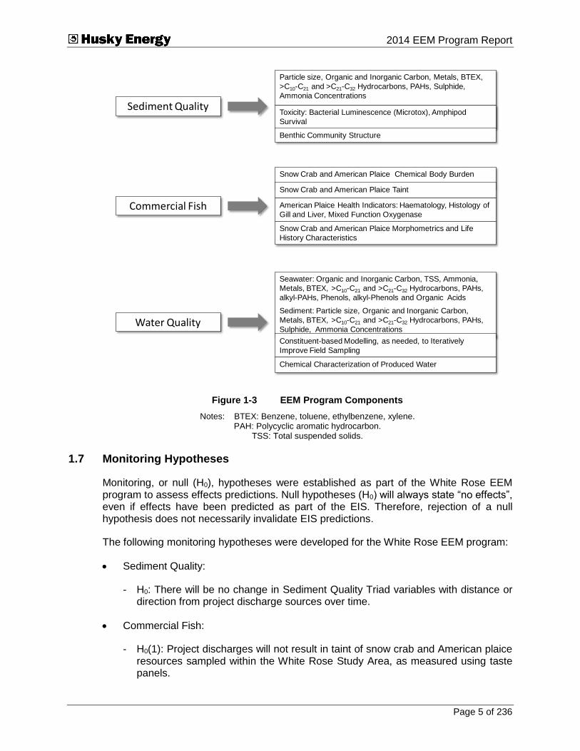
1.6 EEM Program Components and Monitoring Variables
The White Rose EEM program is divided into three components: Sediment Quality, Commercial Fish and Water Quality (Figure 1-3).
Assessment of Sediment Quality includes measurement of alterations in chemical and physical characteristics, measurement of sediment toxicity and assessment of benthic community structure. These three sets of measurements are commonly known as the Sediment Quality Triad (Long and Chapman 1985; Chapman et al. 1987, 1991; Chapman 1992). These tests are used to assess drilling effects (Section 1.5).
Assessment of effects on Commercial Fish species includes measurement of chemical body burden, taint, morphometric and life history characteristics for snow crab (Chionoecetes opilio) and American plaice (Hippoglossoides platessoides) and measurement of various health indices for American plaice.
Assessment of Water Quality includes measurement of alteration of physical and chemical characteristics in the water column and measurement of alterations in sediment chemistry as a result of liquid discharge. Because contamination from liquid discharges from offshore installations is expected to be difficult to detect, constituent-based modelling is also undertaken, as needed, to attempt to identify constituents that would have a higher chance of being detected.
Further details on the selection of monitoring variables are provided in the White Rose EEM Program Design documents (Husky Energy 2004, 2008, 2010a, 2010b, 2014).
Submitted To 2014 EEM Program Report
Page 5 of 236
Particle size, Organic and Inorganic Carbon, Metals, BTEX,
>C10-C21 and >C21-C32 Hydrocarbons, PAHs, Sulphide,
Ammonia Concentrations
Toxicity: Bacterial Luminescence (Microtox), Amphipod
Survival
Benthic Community Structure
Sediment Quality
Commercial Fish
Snow Crab and American Plaice Chemical Body Burden
Snow Crab and American Plaice Taint
American Plaice Health Indicators: Haematology, Histology of
Gill and Liver, Mixed Function Oxygenase
Snow Crab and American Plaice Morphometrics and Life
History Characteristics
Water Quality
Seawater: Organic and Inorganic Carbon, TSS, Ammonia,
Metals, BTEX, >C10-C21 and >C21-C32 Hydrocarbons, PAHs,
alkyl-PAHs, Phenols, alkyl-Phenols and Organic Acids
Sediment: Particle size, Organic and Inorganic Carbon,
Metals, BTEX, >C10-C21 and >C21-C32 Hydrocarbons, PAHs,
Sulphide, Ammonia Concentrations
Constituent-based Modelling, as needed, to Iteratively
Improve Field Sampling
Chemical Characterization of Produced Water
Figure 1-3 EEM Program Components
Notes: BTEX: Benzene, toluene, ethylbenzene, xylene. PAH: Polycyclic aromatic hydrocarbon.
TSS: Total suspended solids.
1.7 Monitoring Hypotheses
Monitoring, or null (H0), hypotheses were established as part of the White Rose EEM program to assess effects predictions. Null hypotheses (H0) will always state “no effects”, even if effects have been predicted as part of the EIS. Therefore, rejection of a null hypothesis does not necessarily invalidate EIS predictions.
The following monitoring hypotheses were developed for the White Rose EEM program:
Sediment Quality:
- H0: There will be no change in Sediment Quality Triad variables with distance or direction from project discharge sources over time.
Commercial Fish:
- H0(1): Project discharges will not result in taint of snow crab and American plaice resources sampled within the White Rose Study Area, as measured using taste panels.
Submitted To 2014 EEM Program Report
Page 6 of 236
- H0(2): Project discharges will not result in adverse effects to fish health within the White Rose Study Area, as measured using histopathology, haematology and Mixed Function Oxygenase (MFO) induction.
Water Quality:
- H0: The distribution of produced water from point of discharge, as assessed using moorings data and/or vessel-based data collection, will not differ from the predicted distribution of produced water.
No hypotheses were developed for American plaice and snow crab chemical body burden and morphometrics and life history characteristics, as these tests were considered to be supporting tests, providing information to aid in the interpretation of results of other monitoring variables (taste tests and health).
1.8 EEM Sampling Design
Sediment samples are collected at stations in the vicinity of drill centres and at a series of stations located at varying distances from drill centres, extending to a maximum of 28 km along north-south, east-west, northwest-southeast and northeast-southwest axes. The sediment sampling design is commonly referred to as a gradient design. This type of design assesses change in monitoring variables with distance from source.
Commercial fish are sampled near White Rose, in the vicinity of the drill centres, and at four distant Reference Areas located approximately 28 km to the northeast, northwest, southeast and southwest.
Water samples are collected in the vicinity of the SeaRose floating, production, storage and offloading (FPSO) vessel (at approximately 300 m), at mid-field stations located 4 km to the southeast of White Rose and in two Reference Areas located approximately 28 km to the northeast and northwest. The sampling designs for water samples and for commercial fish are control-impact designs (Green 1979). This type of design compares conditions near discharge source(s) to conditions in areas unaffected by the discharge(s).
1.8.1 Modifications to the Sediment Component
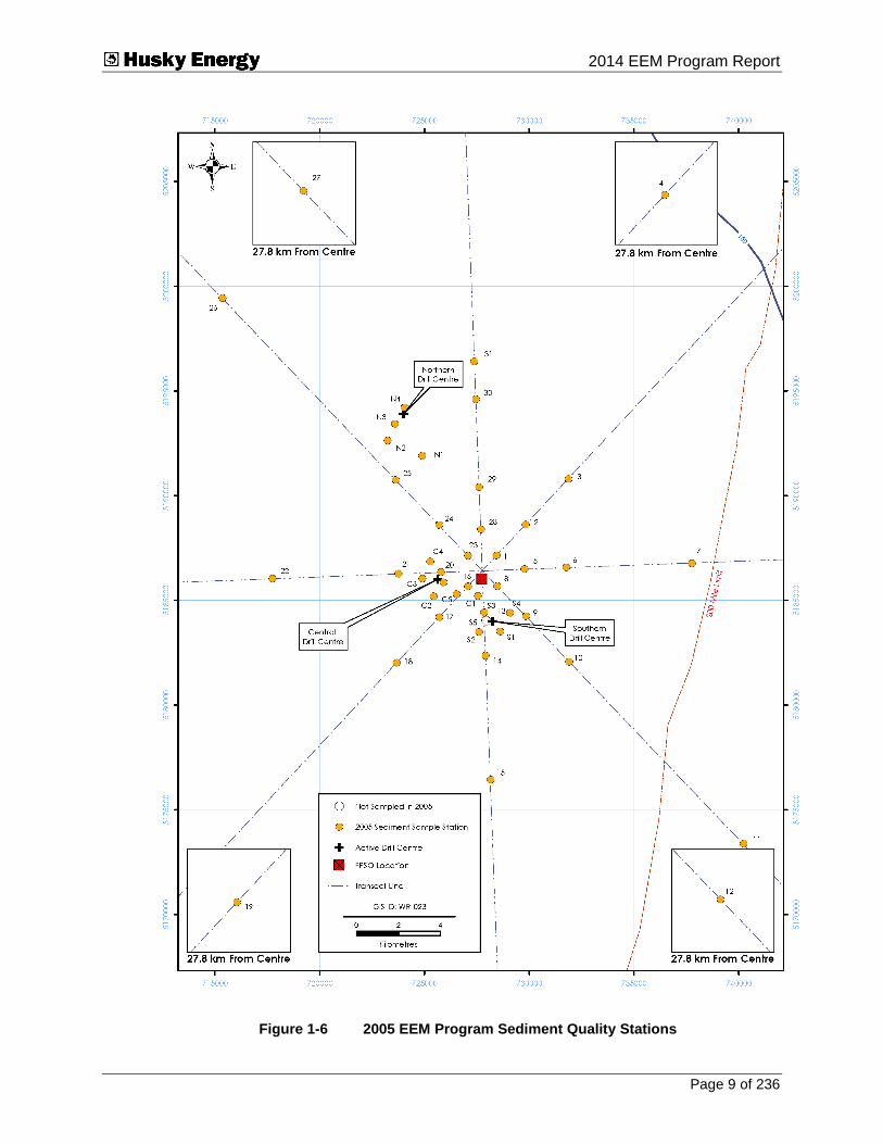
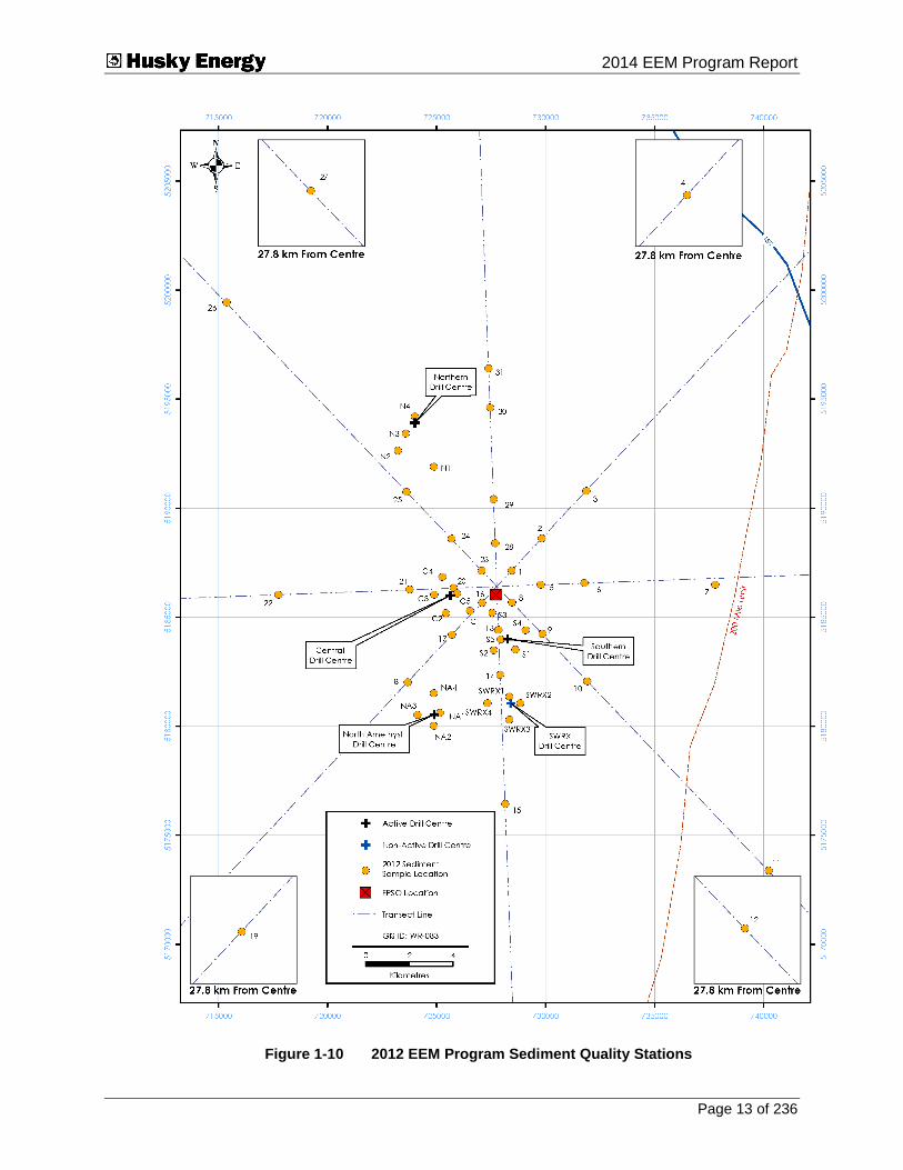
There are some differences between sediment stations sampled for baseline (2000) and for EEM programs (2004, 2005, 2006, 2008, 2010, 2012 and 2014). A total of 48 sediment stations were sampled during baseline (Figure 1-4), 56 stations were sampled for the 2004 EEM program (Figure 1-5), 44 stations were sampled for the 2005 EEM program (Figure 1-6), 59 stations were sampled in 2006 (Figure 1-7), 47 stations were sampled in 2008 (Figure 1-8), 49 stations were sampled in 2010 (Figure 1-9), 53 stations were sampled in 2012 and 2014 (Figures 1-10 and 1-11, respectively). In all, 36 stations were common to all sampling programs.

Submitted To 2014 EEM Program Report
Page 7 of 236
Figure 1-4 2000 Baseline Program Sediment Quality Stations

Submitted To 2014 EEM Program Report
Page 8 of 236
Figure 1-5 2004 EEM Program Sediment Quality Stations
Submitted To 2014 EEM Program Report
Page 9 of 236
Figure 1-6 2005 EEM Program Sediment Quality Stations

Submitted To 2014 EEM Program Report
Page 10 of 236
Figure 1-7 2006 EEM Program Sediment Quality Stations

Submitted To 2014 EEM Program Report
Page 11 of 236
Figure 1-8 2008 EEM Program Sediment Quality Stations

Submitted To 2014 EEM Program Report
Page 12 of 236
Figure 1-9 2010 EEM Program Sediment Quality Stations
Submitted To 2014 EEM Program Report
Page 13 of 236
Figure 1-10 2012 EEM Program Sediment Quality Stations

Submitted To 2014 EEM Program Report
Page 14 of 236
Figure 1-11 2014 EEM Program Sediment Quality Stations

Submitted To 2014 EEM Program Report
Page 15 of 236
As part of EEM program design (Husky Energy 2004, 2008), seven baseline stations in the immediate vicinity of drill centres were eliminated because they were redundant. These stations were sampled during baseline because the final location of the Central, Northern and Southern Drill Centres had not been established. Two remote reference stations located 35 km south-southeast and 85 km northwest of White Rose were eliminated for the EEM programs because of their distance from the development and because sediment chemistry results from baseline sampling showed that the northwest reference station might not be comparable to other stations. Two 18-km stations were eliminated because of redundancies with other stations (see Husky Energy 2004 for details).
Original station additions for the EEM program included four reference stations at 28 km from the centre of the development, one station along the north axis at approximately 8 km from the centre of the development and three drill centre stations located approximately 300 m from each of the Northern, Central and Southern Drill Centres. However, in 2005, one of these stations (station S5) could not be sampled because of drilling activity at the Southern Drill Centre.
In 2004, six drill centre stations were sampled at 1 km from the proposed location of each of more northerly (NN) and more southerly (SS) drill centres to provide additional baseline data should drilling occur at these drill centres (see Figure 1-5). Since there are no immediate plans to drill at these drill centres, these stations were not sampled in subsequent programs. Similarly, 14 ‘West’ stations were sampled in 2006 around the proposed location of the West-Alpha and West-Bravo Drill Centres located to the northwest of the Central Drill Centre (Figure 1-7).
In 2008, four new stations were added to the EEM program around the North Amethyst Drill Centre (Figure 1-8). These four stations, along with stations 14 and 18, were also sampled in 2007 to provide additional pre-drilling baseline information for that drill centre.
In 2010, stations NA1, NA4, C5 and 23 were moved slightly because of proximity to subsea infrastructure. NA4, 23 and C5 were relocated less than 15 m from the original locations. NA1 was relocated approximately 85 m from its original location but at the same distance from the drill centre as the original location.
In 2012, four stations were added around the SWRX Drill Centre (Figure 1-10) and stations 23, 25, C5, NA1, NA3 and N4 were moved slightly because of proximity to subsea infrastructure. All stations were moved less than 50 m from their original location.
In 2014, stations C1 and C5 were moved slightly because of proximity to subsea infrastructure. All stations were moved less than 50 m from their original location.
Table 1-1 provides a summary of changes between the 2000 baseline program and the 2014 EEM program for sediment, as well as station name changes that were proposed in the EEM design document to simplify reporting of results.

Submitted To 2014 EEM Program Report
Page 16 of 236
Table 1-1 Table of Concordance between Baseline and 2014 EEM Sediment Stations
EEM Program Station Name Corresponding Station Name during the 2000 Baseline Program
1 F1-1,000
2 F1-3,000
3 F1-6,000
4 Not Sampled in 2000
5 F2-2,000
6 F2-4,000
7 F2-10,000
8 F3-1,000
9 F3-3,000
10 F3-6,000
11 F3-18,000
12 Not Sampled in 2000
13 F4-2,000
14 F4-4,000
15 F4-10,000
16 F5-1,000
17* F5-3,000
18 F5-6,000
19 Not Sampled in 2000
20 F6-2,000
21 F6-4,000
22 F6-10,000
23 F7-1,000
24 F7-3,000
25 F7-6,000
26 F7-18,000
27 Not Sampled in 2000
28 F8-2,000
29 F8-4,000
30 F8-10,000
31 Not Sampled in 2000
C1 GH2-3
C2 GH2-4
C3 GH2-5
C4 GH2-6
C5* Not Sampled in 2000
N1 GH3-3
N2 GH3-5
N3 GH3-6
N4 Not Sampled in 2000
S1 GH1-3
S2 GH1-4
S3 GH1-6
S4 GH1-2
S5** Not Sampled in 2000
NA1 Not Sampled in 2000
NA2 Not Sampled in 2000
NA3 Not Sampled in 2000
NA4 Not Sampled in 2000
SWRX1 Not Sampled in 2000
SWRX2 Not Sampled in 2000
SWRX3 Not Sampled in 2000
SWRX4 Not Sampled in 2000
Notes: - For 2000 baseline stations, only those stations retained for the EEM program are listed. - Additional baseline stations sampled in 2004 and 2006 are not listed in the above Table; see text and
figures for details. - *Not sampled in 2008 because of drilling activity; ** Not sampled in 2005 because of drilling activity.

Submitted To 2014 EEM Program Report
Page 17 of 236
1.8.2 Modifications to the Commercial Fish Component
For American plaice and snow crab, sampling for the baseline program (2000 and 2002) occurred near White Rose and in one Reference Area located 85 km to the northwest. For the EEM program, this Reference Area was replaced with four Reference Areas located approximately 28 km northwest, northeast, southwest and southeast of the development. Figures 1-12 to 1-18 provide transect locations for the 2004, 2005, 2006, 2008, 2010, 2012 and 2014 EEM programs, respectively. The fisheries exclusion zone was larger in 2004 than in 2005 and 2006 to accommodate possible drilling at the NN and SS Drill Centres. The zone was again increased in size in 2008 and 2010, from 2005 and 2006, to accommodate the North Amethyst Drill Centre. In 2008, heavy commercial fishing activity for crab in Reference Areas 3 and 4 precluded sampling. In 2012, the approved White Rose safety zone was used as the boundary for fishing, and that area was expanded in 2014 to accommodate the SWRX Drill Centre.

Submitted To 2014 EEM Program Report
Page 18 of 236
Figure 1-12 2004 EEM Program Commercial Fish Transect Locations

Submitted To 2014 EEM Program Report
Page 19 of 236
Figure 1-13 2005 EEM Program Commercial Fish Transect Locations

Submitted To 2014 EEM Program Report
Page 20 of 236
Figure 1-14 2006 EEM Program Commercial Fish Transect Locations

Submitted To 2014 EEM Program Report
Page 21 of 236
Figure 1-15 2008 EEM Program Commercial Fish Transect Locations
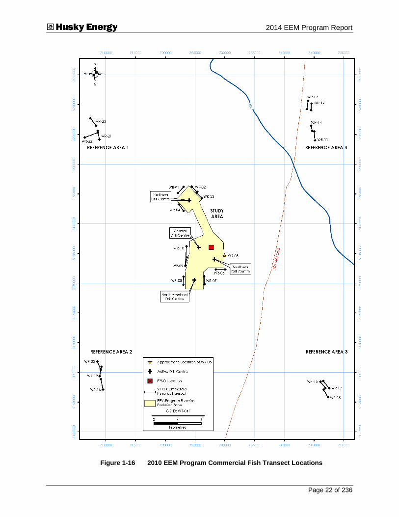
Submitted To 2014 EEM Program Report
Page 22 of 236
Figure 1-16 2010 EEM Program Commercial Fish Transect Locations

Submitted To 2014 EEM Program Report
Page 23 of 236
Figure 1-17 2012 EEM Program Commercial Fish Transect Locations

Submitted To 2014 EEM Program Report
Page 24 of 236
Figure 1-18 2014 EEM Program Commercial Fish Transect Locations

Submitted To 2014 EEM Program Report
Page 25 of 236
1.8.3 Modifications to the Water Quality Component
The Water Quality Component of the White Rose EEM targets both seawater and sediments as receiving environments for constituents from liquid discharge, predominantly produced water, from White Rose.
1.8.3.1 Seawater Samples
Water samples were collected at 13 randomly selected stations during baseline sampling in 2000 (Figure 1-194). Produced water discharge began from the SeaRose FPSO in March 2007. A preliminary EEM water sampling program was executed in 2008, with eight stations near the SeaRose FPSO (the main source of liquid discharge) and one station located approximately 28 km to the northwest (Figure 1-20). A greater number of stations (18) were sampled in 2010, with 10 stations located near the SeaRose FPSO and eight stations located in Reference Areas to northwest and northeast (Figure 1-21). Modelling was used in the 2010 program to assess the probability of detection of produced water constituents in seawater given anticipated dilution and laboratory detection limits. The Water Quality program then was modified based on modelling, as well as field results. Sampling of radionuclides (sampled in seawater) was discontinued in 2012. Sampling of selected process chemicals in seawater was discontinued in 2014. In 2012 and 2014, five stations were sampled near the SeaRose FPSO in the direction of winds and currents at the time of sampling; five stations were sampled in the mid-field (4 km from the SeaRose FPSO) in the direction of the prevailing seasonal current; and the same eight stations sampled in Reference Areas in 2010 were again sampled in 2012 and 2014 (Figures 1-22 and 1-23, respectively). Since 2010, EEM water samples have been processed for a larger number of constituents and at lower detection limits than in baseline (see Section 7 and Husky Energy 2010a for details).
1.8.3.2 Sediment Samples
In 2010, stations sampled for seawater (Figure 1-21) were also sampled for sediment particle size and sediment chemistry, including radionuclide concentration. Thirteen stations sampled as part of the Sediment Component of the EEM program were also sampled for radionuclide concentrations, for a total of 27 radionuclide stations.
In 2012, a modelling exercise examined the probability of detection of produced water radionuclides in sediments. Based on model results, sampling of sediment radionuclides was discontinued in 2012 (also see Section 7), but all other analyses on sediments at Water Quality stations (Figure 1-20) were retained.
4 Figure 1-19 excludes water samples collected at the two control stations sampled during baseline and
subsequently excluded from the EEM sampling.

Submitted To 2014 EEM Program Report
Page 26 of 236
Figure 1-19 2000 Baseline Program Water Quality Stations
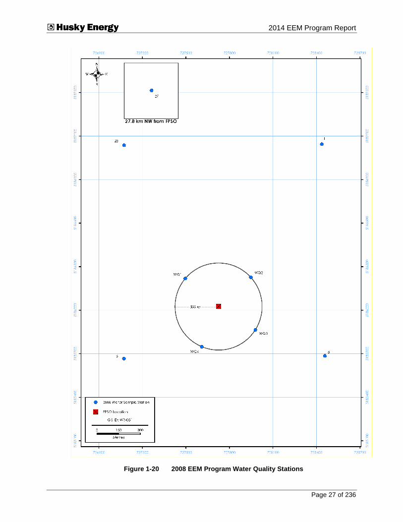
Submitted To 2014 EEM Program Report
Page 27 of 236
Figure 1-20 2008 EEM Program Water Quality Stations

Submitted To 2014 EEM Program Report
Page 28 of 236
Figure 1-21 2010 EEM Program Water Quality Stations

Submitted To 2014 EEM Program Report
Page 29 of 236
Figure 1-22 2012 EEM Program Water Quality Stations
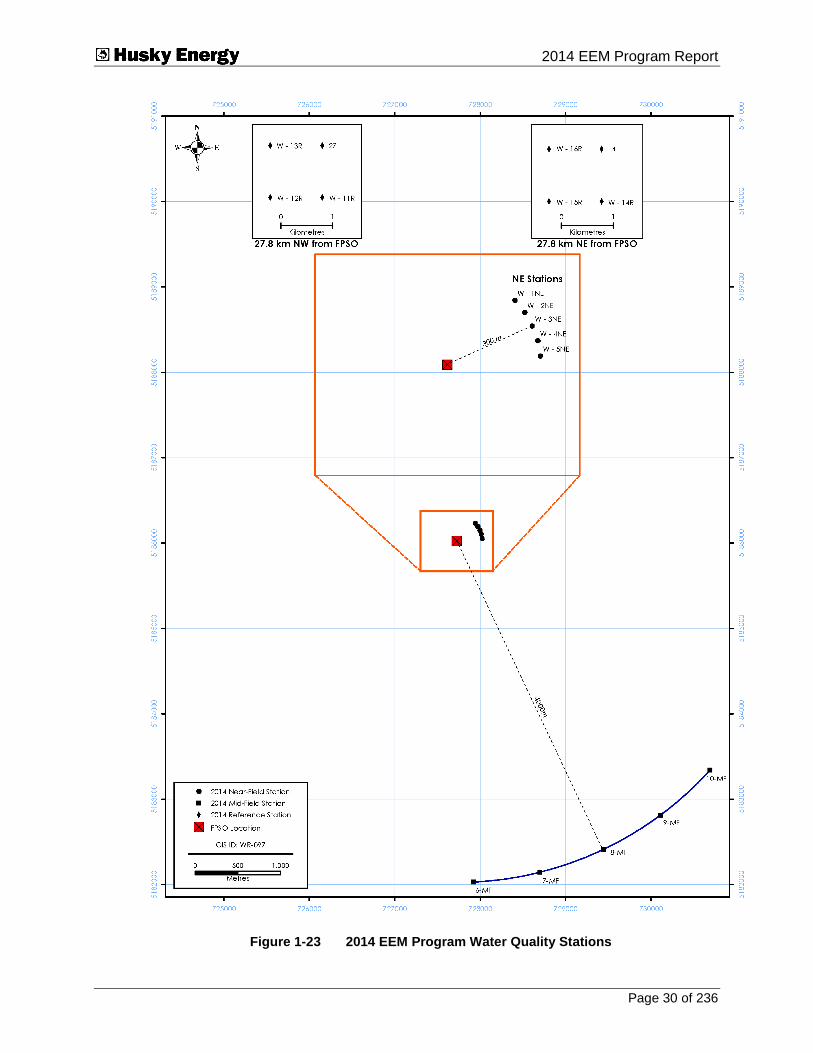
Submitted To 2014 EEM Program Report
Page 30 of 236
Figure 1-23 2014 EEM Program Water Quality Stations

Submitted To 2014 EEM Program Report
Page 31 of 236
2.0 Scope
This document, White Rose Environmental Effects Monitoring Program 2014 (Volume 1), provides summary results, analysis and interpretation for the White Rose 2014 EEM program. Where applicable, results from the baseline and previous EEM programs are compared to 2014 results. Since analyses of results are often highly technical, a summary of findings section is included at the end of each results section. The discussion section of the report provides interpretation of results and an overall assessment of potential project effects with respect to monitoring hypotheses (Section 1.7).
Most methods are provided in Volume 1. However, some more detailed methods as well as ancillary analyses are included in Appendices (White Rose Environmental Effects Monitoring Program 2014 (Volume 2)). Raw data and other information supporting Volume 1 are also provided in Volume 2.
2.1 Background Material
The executive summary and discussion section of this document are written for a general audience. The methods and results sections assume a certain level of understanding of EEM, survey design and statistical analysis. References to statistical methods used are provided in the reference section of this document. The most useful references, as well as other standard references, are provided below.
Armsworthy, S.L., P.J. Cranford and K. Lee (Editors). 2005. Offshore Oil and Gas Environmental Effects Monitoring: Approaches and Technologies. Battelle Press, Columbus, OH. xvi + 631 pp.
DeBlois, E.M., J.W. Kiceniuk, M.D. Paine, B.W. Kilgour, E. Tracy, R.D. Crowley, U.P. Williams, G.G. Janes. 2014. Examination of body burden and taint for Iceland scallop (Chlamys islandica) and American plaice (Hippoglossoides platessoides) near the Terra Nova offshore oil development over ten years of drilling on the Grand Banks of Newfoundland, Canada. Deep-Sea Research II, 110: 65-83.
DeBlois, E.M., M.D. Paine, B.W. Kilgour, E. Tracy, R.D. Crowley, U.P. Williams and G.G. Janes. 2014. Alterations in bottom sediment physical and chemical characteristics at the Terra Nova offshore oil development over ten years of drilling on the Grand Banks of Newfoundland, Canada. Deep-Sea Research II, 110: 13-25.
Ellis, J.L. and D.C. Schneider. 1997. Evaluation of a gradient design for environmental impact assessment. Environmental Monitoring and Assessment, 48: 157-172.
Environment Canada. 1998. Reference Method for Determining Acute Lethality of Sediment to Marine or Estuarine Amphipods. Report EPS 1/RM/35. Environment Canada Environmental Protection Service, Ottawa, ON. xviii + 56 pp.
Environment Canada. 2002. Biological Test Method: Reference Method for Determining the Toxicity of Sediment Using Luminescent Bacteria in a Solid-Phase Test. Report EPS 1/RM/42. xxii + 60 pp.
Submitted To 2014 EEM Program Report
Page 32 of 236
Environment Canada. 2010. Pulp and Paper Environmental Effects Monitoring (EEM) Technical Guidance Document. http://www.ec.gc.ca/Publications/7CCC415A-FE25-4522-94E4-024B9F3EAE7E%5CPP_full_versionENGLISH%5B1%5D-FINAL-2.0.pdf
Gilbert, R.O. 1987. Statistical Methods for Environmental Pollution Monitoring. Van Nostrand Reinhold, New York, NY. 320 pp.
Green, R.H. 1979. Sampling Design and Statistical Methods for Environmental Biologists. John Wiley and Sons, Toronto, ON. 257 pp.
Green, R.H. 1993. Application of repeated-measures design in environmental impact and monitoring studies. Australian Journal of Ecology, 18: 81-98.
Green, R.H., J.M. Boyd and J.S. Macdonald. 1993. Relating sets of variables in environmental studies: The Sediment Quality Triad as a paradigm. Environmetrics, 44: 439-457.
Ludwig, J.A. and J.F. Reynolds. 1988. Statistical Ecology: A Primer on Methods and Computing. John Wiley & Sons, New York, NY. 337 pp.
Paine, M.D., E.M. DeBlois, B.W. Kilgour, E. Tracy, P. Pocklington, R.D. Crowley, U.P. Williams, G.G. Janes. 2014. Effects of the Terra Nova offshore oil development on benthic macro-invertebrates over 10 years of development drilling on the Grand Banks of Newfoundland, Canada. Deep-Sea Research II, 110: 38-64.
Paine, M.D., M.A. Skinner, B.W. Kilgour, E.M. DeBlois, E. Tracy. 2014. Repeated-measures regression designs and analysis for environmental effects monitoring programs. Deep-Sea Research II, 110: 84-91.
Quinn, G.P. and M.J. Keough. 2002. Experimental Design and Data Analysis for Biologists. Cambridge University Press, Cambridge, UK. 537 pp.
Schmitt, R.J. and C. W. Osenberg (Editors). 1996. Detecting Ecological Impacts: Concepts and Applications in Coastal Habitats. Academic Press, San Diego, CA. 401 pp.
van Belle, G. 2002. Statistical Rules of Thumb. John Wiley & Sons, New York, NY. 221 pp. (more recent rules of thumb are posted at http://www.vanbelle.org).
Various Authors. 1996. Canadian Journal of Fisheries and Aquatic Science, Volume 53(11) (this volume provides reviews of GOOMEX studies).
Whiteway, S.A., M.D. Paine, T.A. Wells, E.M. DeBlois, B.W. Kilgour, E. Tracy, R.D. Crowley, U.P. Williams and G.G. Janes. 2014. Toxicity assessment in marine sediments for the Terra Nova environmental effects monitoring program (1997 -2010). Deep-Sea Research II, 110: 26-37.

Submitted To 2014 EEM Program Report
Page 33 of 236
3.0 Abbreviations, Acronyms and Units of Measure
The following abbreviations, acronyms and units of measure are used in this report.
Abbreviations Definition
°C degrees Celsius
#/m² number [of organisms] per square metre
ANCOVA Analysis of Covariance
ANOVA Analysis of Variance
Bq/g Becquerel per gram
BTEX benzene, toluene, ethylbenzene and xylenes
CCME Canadian Council of Ministers of the Environment
cm centimetre
C-NLOPB Canada-Newfoundland and Labrador Offshore Petroleum Board
DFO Fisheries and Oceans Canada
EEM environmental effects monitoring
EIS Environmental Impact Statement
EPCMP Environmental Protection and Compliance Monitoring Plan
EROD 7-ethoxyresorufin O-deethylase
FPSO floating, production, storage and offloading vessel
g gram
g/kg gram per kilogram
g/m² gram per square metre
H0 null hypothesis
HOIMS Husky Operational Integrity Management System
ISQG Interim Sediment Quality Guidelines
kg kilogram
km kilometre
km² square kilometre
L litre
L/s litre per second
m metre
m² square metre
m³ cubic metre
MFO Mixed Function Oxygenase
mg milligram
mg/kg milligram per kilogram
mg/L milligram per litre
ml millilitre
mm millimetre
mV millivolts
PAH polycyclic aromatic hydrocarbon
PCA Principal Component Analysis
ppm parts per million
QA/QC quality assurance/quality control
SD standard deviation
SWRX South White Rose Extension
TIC total inorganic carbon

Submitted To 2014 EEM Program Report
Page 34 of 236
Abbreviations Definition
TOC total organic carbon
TSS total suspended sediment
µg/L microgram per litre

Submitted To 2014 EEM Program Report
Page 35 of 236
4.0 Project Activities
4.1 Introduction
This section reports on both drilling and production activities in the White Rose Field and summarizes the authorized discharges associated with these operations.
Husky’s Environmental Protection and Compliance Monitoring Plan (EPCMP) describes the environmental protection measures and compliance monitoring requirements applicable to Husky’s drilling and production related operations. The EPCMP is prepared in alignment with the C-NLOPB’s Environmental Protection Plan Guidelines, Offshore Waste Treatment Guidelines, Drilling and Production Guidelines and all other applicable regulatory requirements. The EPCMP has its basis in the Husky Operational Integrity Management System (HOIMS), and is responsive to the C-NLOPB’s regulatory approval process and other relevant regulatory requirements.
The purpose of this section is to provide context for the interpretation of the results from the EEM program.
4.2 Project Activities
Activities associated with the White Rose Development Project to date fall into five general categories:
construction and installation operations for the original White Rose Field were completed in Fall 2005 (see Husky Energy 2006); flowlines and protective berms were installed to connect the North Amethyst Drill Centre to the Southern Drill Centre in 2009;
A new drill centre at SWRX was excavated in 2012. In 2013, a gas injection flowline from the Northern Drill Centre was tied-in directly to the SWRX Drill Centre. In 2014, the SWRX Drill Centre was tied back to the existing production, water injection and gas lift flowlines from the North Amethyst Drill Centre and the Southern Drill Centre.
drilling operations including development, and delineation drilling in the White Rose field (ongoing for the foreseeable future by one or more drilling platforms);
SeaRose FPSO operations (ongoing for the foreseeable future); and
supply vessel operations (ongoing for the foreseeable future).
Production operations (i.e., oil and gas production, storage and offloading to a tanker) began at the White Rose Field once hook-up, commissioning and introduction of hydrocarbons to the SeaRose FPSO were completed in November of 2005. In May 2010, White Rose started producing from the North Amethyst Drill Centre. Production from the SWRX drill centre began in June, 2015. Since the last EEM in August 2012, the SeaRose FPSO was shut down for maintenance from August 21 to 28, 2014, during which time there was no production-related discharge.

Submitted To 2014 EEM Program Report
Page 36 of 236
4.3 Drilling and Completions Operations
Drilling activities continued since the last round of EEM sampling in August 2012 through to the latest EEM sampling in October 2014. Husky uses both water-based drill muds and synthetic fluid-based drill muds in its drilling programs. Water-based drill muds are used for the upper two drill hole sections, which is riserless drilling, while synthetic fluid-based drill muds are used in deeper hole sections, especially during directional drilling operations, where drilling conditions are more difficult and hole stability is critical to safety and success.
HOIMS and Husky’s Waste Management Procedures commit to an active program to manage the generation, reuse or recycling and disposal of waste materials generated by any of Husky’s Atlantic Region offshore or onshore operations.
This is achieved through the following objectives:
limit or minimize the waste generated from East Coast operations; and
all waste from East Coast operations is handled in an environmentally responsible manner.
There are several tools currently in place to assist with the implementation of these objectives:
White Rose Waste Management Plan (EC-M-99-X-PR-00109-001);
SeaRose Waste Management Procedure (WR-O-00-X-PR-00001-001);
internal reviews of waste manifesting procedures; and
management of key contractors.
4.3.1 Drilling Mud and Completion Fluids Discharges
Table 4-1 summarizes the volumes of drill cuttings and water-based drill muds discharged during development drilling activities by year and drill centre. The months during which drilling activities took place are also indicated.
Table 4-2 summarizes the volumes of drill cuttings and synthetic fluid-based drill muds discharged during development drilling activities by year and drill centre. The months during which drilling activities took place are also indicated.
Upon completion, a well bore needs to be cleaned of residual cuttings. This is done by flushing with “completion fluids”, consisting primarily of sodium chloride or potassium formate brines. Table 4-3 summarizes the volumes of completion fluids discharged during well completions by year and drill centre. The months during which these activities took place are also indicated.
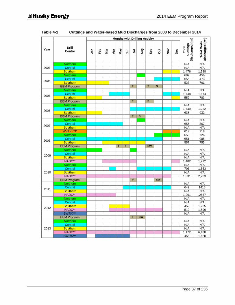
Submitted To 2014 EEM Program Report
Page 37 of 236
Table 4-1 Cuttings and Water-based Mud Discharges from 2003 to December 2014
Year Drill
Centre
Months with Drilling Activity
To
tal
Cu
ttin
gs
Dis
ch
arg
ed
(m
t)
To
tal M
ud
s
Dis
ch
arg
ed
(m
³)
Jan
Fe
b
Ma
r
Ap
r
Ma
y
Ju
n
Ju
l
Au
g
Sep
Oct
No
v
Dec
2003
Northern N/A N/A
Central N/A N/A
Southern 1,476 1,588
2004
Northern 682 456
Central 655 473
Southern 537 761
EEM Program F S S
2005
Northern N/A N/A
Central 1,748 1,674
Southern 552 783
EEM Program F S
2006
Northern N/A N/A
Central 1,749 1,282
Southern 638 932
EEM Program F S
2007
Northern N/A N/A
Central 655 867
Southern N/A N/A
Well K 03* 619 718
2008
Northern 653 726
Central 651 985
Southern 557 753
EEM Program F F SW
2009
Northern N/A N/A
Central N/A N/A
Southern N/A N/A
NADC** 1,482 1,772
2010
Northern N/A N/A
Central 706 1,553
Southern N/A N/A
NADC** 1,331 2,703
EEM Program F SW
2011
Northern N/A N/A
Central 649 1413
Southern N/A N/A
NADC** 1,261 ,2557
2012
Northern N/A N/A
Central N/A N/A
Southern 459 1,285
NADC** 512 1,596
SWRX*** N/A N/A
EEM Program F SW
2013
Northern N/A N/A
Central N/A N/A
Southern N/A N/A
NADC** 1,172 6,480
SWRX*** 458 1,620

Submitted To 2014 EEM Program Report
Page 38 of 236
Year Drill
Centre
Months with Drilling Activity
To
tal
Cu
ttin
gs
Dis
ch
arg
ed
(m
t)
To
tal M
ud
s
Dis
ch
arg
ed
(m
³)
Jan
Fe
b
Ma
r
Ap
r
Ma
y
Ju
n
Ju
l
Au
g
Sep
Oct
No
v
Dec
2014
Northern N/A N/A
Central N/A N/A
Southern N/A N/A
NADC** 0 90
SWRX*** 641 3,704
EEM Program F SW
Total Discharge at Northern Drill Centre 1,335 1,182
Total Discharge at Central Drill Centre 6,813 8,247
Total Discharge at Southern Drill Centre 4,219 6,102
Total Discharge at NADC** 5,758 15,198
Total Discharge at SWRX*** 1,099 5,324
Total Field Discharge 19,224 36,053
Note: - * Well K 03 is a Delineation Well. - ** NADC – North Amethyst Drill Centre. - *** SRWX – South White Rose Drill Centre. - F = Commercial Fish portion of the EEM program. - S = Sediment Quality portion of the EEM program. - W = Water Quality portion of the EEM program. - mt = metric tonne - m³ = cubic metre
Table 4-2 Cuttings and Synthetic-based Mud Discharges from 2003 to December 2014
Year Drill
Centre
Months with Drilling Activity
To
tal
Cu
ttin
gs
Dis
ch
arg
ed
(m
t)
To
tal S
olid
s
Dis
ch
arg
ed
(m
t)
To
tal
Base O
il
Dis
ch
arg
ed
(m
³)
Jan
Fe
b
Ma
r
Ap
r
Ma
y
Ju
n
Ju
l
Au
g
Sep
Oct
No
v
Dec
2003
Northern N/A N/A N/A
Central N/A N/A N/A
Southern 416 957 228
2004
Northern 350 473.1 35
Central 253 1,197 141
Southern 1,193 3,358 512
EEM Program F S S
2005
Northern N/A N/A N/A
Central 1,291 2,382 482
Southern 741 1,464 157
EEM Program F S
2006
Northern N/A N/A N/A
Central 1,268 3,163 335
Southern 1,028 1,927 185
EEM Program F S
2007
Northern 409 719.9 71
Central 1,291 2,382 241
Southern N/A N/A N/A
Well K 03* 437 775 65
2008
Northern 771 1,765.6 202
Central 483 979 88
Southern 668 1,518 151
EEM Program F F SW
2009
Northern 106 186 22
Central N/A N/A N/A
Southern N/A N/A N/A
NADC** 752 1,345 117

Submitted To 2014 EEM Program Report
Page 39 of 236
Year Drill
Centre
Months with Drilling Activity
To
tal
Cu
ttin
gs
Dis
ch
arg
ed
(m
t)
To
tal S
olid
s
Dis
ch
arg
ed
(m
t)
To
tal
Base O
il
Dis
ch
arg
ed
(m
³)
Jan
Fe
b
Ma
r
Ap
r
Ma
y
Ju
n
Ju
l
Au
g
Sep
Oct
No
v
Dec
2010
Northern N/A N/A N/A
Central 524 1,141 106
Southern N/A N/A N/A
NADC** 1,034 3,149 223
EEM Program F SW
2011
Northern N/A N/A N/A
Central 429 1,392 101
Southern N/A N/A N/A
NADC** 799 1,309 111
2012
Northern N/A N/A N/A
Central N/A N/A N/A
Southern 732 847 185
NADC** 853 907 148
SWRX*** N/A N/A N/A
EEM Program F SW
2013
Northern N/A N/A N/A
Central N/A N/A N/A
Southern N/A N/A N/A
NADC** 1,465 2,362 210
SWRX*** 712 1,761 160
2014
Northern N/A N/A N/A
Central N/A N/A N/A
Southern N/A N/A N/A
NADC** 814 1,459 103
SWRX*** 284 563 17
EEM Program F SW
Total Discharge at Northern Drill Centre 1,636 3,144 330
Total Discharge at Central Drill Centre 5,539 12,636 1,494
Total Discharge at Southern Drill Centre 4,778 10,071 1,418
Total Discharge at NADC** 5,717 10,531 912
Total Discharge at SWRX*** 996 2,324 177
Total Field Discharge 18,666 38,706 4,331
Notes: - * Well K 03 is a Delineation Well. - ** NADC – North Amethyst Drill Centre. - *** SWRX – South White Rose Extension Drill Centre. - F = Commercial Fish portion of the EEM program. - S = Sediment Quality portion of the EEM program. - W = Water Quality Portion of the EEM program. - mt = metric tonne - m³ = cubic metre
Table 4-3 Completion Fluid Discharges from 2003 to December 2014
Year Drill
Centre
Months with Drilling Activity
To
tal
Co
mp
leti
on
Flu
ids
Dis
ch
arg
ed
(m
³)
Jan
Fe
b
Ma
r
Ap
r
Ma
y
Ju
n
Ju
l
Au
g
Sep
Oct
No
v
Dec
2003
Northern N/A
Central N/A
Southern N/A
2004
Northern N/A
Central N/A
Southern 1,619
EEM Program

Submitted To 2014 EEM Program Report
Page 40 of 236
Year Drill
Centre
Months with Drilling Activity
To
tal
Co
mp
leti
on
Flu
ids
Dis
ch
arg
ed
(m
³)
Jan
Fe
b
Ma
r
Ap
r
Ma
y
Ju
n
Ju
l
Au
g
Sep
Oct
No
v
Dec
2005
Northern F S S N/A
Central 1,015
Southern 1,372
EEM Program F S
2006
Northern N/A
Central 901.1
Southern 476
EEM Program F S
2007
Northern 150
Central 573
Southern N/A
Well K 03* N/A
2008
Northern N/A
Central 186
Southern 250
EEM Program F F SW
2009
Northern 235
Central N/A
Southern N/A
NADC** 29
2010
Northern N/A
Central N/A
Southern N/A
NADC** 2,293
EEM Program F SW
2011
Northern N/A
Central 673
Southern N/A
NADC** 821
2012
Northern N/A
Central 445
Southern 597
NADC** 592
SWRX*** N/A
EEM Program F SW
2013
Northern N/A
Central N/A
Southern N/A
NADC** 838
SWRX*** 359
2014
Northern N/A
Central N/A
Southern N/A
NADC** N/A
SWRX*** 103
EEM Program F SW
Total Discharge at Northern Drill Centre 385
Total Discharge at Central Drill Centre 3,793
Total Discharge at Southern Drill Centre 4,314
Total Discharge at NADC** 4,573
Total Discharge at SWRX*** 462
Total Field Discharge 13,527
Notes: - * Well K 03 is a Delineation Well. - ** NADC – North Amethyst Drill Centre. - *** SWRX – South White Rose Extension Drill Centre. - F = Commercial Fish portion of the EEM program. - S = Sediment Quality portion of the EEM program. - W = Water Quality portion of the EEM program. - m³ = cubic metre

Submitted To 2014 EEM Program Report
Page 41 of 236
4.3.2 Other Discharges from Drilling Operations
Between November 2012 and September 2014, a total of 526.7 m³ of bilge water from drilling operations was discharged. All bilge water is treated in an oily water separator prior to release to reduce hydrocarbon content to 15 ppm or less in accordance with Husky’s EPCMP. In total, 7.8 kg of hydrocarbons were released to the marine environment from bilge water. Similarly, all deck drainage is collected and treated to reduce hydrocarbon content to 15 ppm or less. However, there was no deck drainage discharged to the marine environment during this period.
Water and ethylene glycols are routinely discharged during function testing of a seabed blowout preventer and subsea flowline valves. In total, over the reporting period between November 2012 and September 2014, approximately 171.1 m³ of water and glycols have been discharged from these sources, at between 25% and 35% of total volume, approximately 51.2 m³ of which have been active ingredients.
4.4 SeaRose FPSO Production Operations
The primary points of hydrocarbon discharge to the marine environment from the SeaRose FPSO are the bilge, the slops tanks and produced water. Bilge water on the SeaRose FPSO is typically directed towards the slops tanks to discharge. Slops tanks are reservoirs for collecting both rainwater (washed over the production facility from open and closed drains) and the redirected bilge water. Contents of the slops tanks undergo oil/water separation and testing prior to discharge to a level of less than 15 ppm hydrocarbon, as per Husky’s EPCMP. Between November 2012 and September 2014, a total of 17,531 m³ of water was released from the slops tanks, representing 57.32 kg (average 3.25 ppm) of hydrocarbons to the marine environment.
Produced water is a by-product of oil production and is a combination of water entrained within the reservoir (formation) and seawater injected into the reservoir to maintain pressure. Produced water is removed from crude oil through a series of separation processes in the production train. Produced water has two regulatory limits for oil in water, as per Husky’s EPCMP: a 24-hour arithmetic mean less than 44 ppm; and a volume-weighted 30-day rolling average less than 30 ppm. Between November 2012 and September 2014, 7,663,485 m³ of produced water was released, representing 106,111 kg (average for end-of month 30-day rolling average was 13.85 ppm) of hydrocarbons to the marine environment.
Seawater is pumped aboard the SeaRose FPSO and is circulated around equipment as cooling water to reduce operating temperatures. To prevent biofouling within the cooling water system, the seawater is treated with chlorine and is managed such that the residual chlorine level at discharge is 1.0 ppm or less, approximately the same as drinking water. Between November 2012 and September 2014, the monthly average concentration of chlorine prior to release was 0.23 ppm.

Submitted To 2014 EEM Program Report
Page 42 of 236
4.5 Supply Vessel Operations
All offshore facilities and operations are supported by supply and standby vessels. Normal vessel operations involve discharge of both treated sewage and bilge water. Bilge water from vessels is treated such that it contains 15 ppm or less of dispersed oil and is released in accordance with the International Convention for the Prevention of Pollution from Ships (MARPOL 73/78) requirements.

Submitted To 2014 EEM Program Report
Page 43 of 236
5.0 Sediment Component
5.1 Methods
5.1.1 Field Collection
The Sediment Component of the 2014 EEM Program was conducted from October 31 to November 4, 2014, using the offshore supply vessel Atlantic Raven. Sampling dates for the baseline program and EEM programs are summarized in Table 5-1. Sediment stations for the baseline and EEM programs are shown in Figures 1-4 to 1-10 (Section 1), with the 2014 station locations provided again in Figure 5-1. Differences in sampling locations among years are described in Section 1. More details on the baseline survey and the Year 1, 2 3, 4, 5 and 6 EEM programs can be found in Husky Energy (2001; 2005; 2006; 2007; 2009; 2011; 2013). Geographic coordinates and distances to drill centres for EEM stations sampled in 2014 are provided in Appendix B-1.
Table 5-1 Date of Sediment Field Programs
Trip Date
Baseline Program September 9 to September 19, 2000
EEM Program Year 1 September 26 to October 11, 2004
EEM Program Year 2 September 16 to September 22, 2005
EEM Program Year 3 August 14 to August 18, 2006
EEM Program Year 4 September 17 to September 21, 2008
EEM Program Year 5 October 4 to October 13, 2010
EEM Program Year 6 August 21 to August 26, 2012
EEM Program Year 7 October 31 to November 4, 2014
Sediment was collected using a large-volume corer (mouth diameter = 35.6 cm, depth = 61 cm) designed to mechanically take an undisturbed sediment sample over approximately 0.1 m² (0.0995 m²) of seabed (Figures 5-2 and 5-3). Sediment oxidation/ reduction potential (redox) was measured on each sediment core before sample collection. In 2014, sediment quality stations were sampled for physical and chemical characteristics, toxicity and benthic community structure. These three sets of variables constitute the Sediment Quality Triad (see Section 1). Physical and chemical characteristics variables included particle size, total organic carbon (TOC) and total inorganic carbon (TIC), metals, total petroleum hydrocarbons, benzene, toluene, ethylbenzene, xylene (BTEX), and >C10-C21 and >C21-C32 hydrocarbons), polycyclic aromatic hydrocarbons (PAHs), sulphur, sulphide, ammonia and moisture. Toxicity variables included bacterial luminescence and amphipod survival. Benthic community variables included total abundance, biomass and richness.

Submitted To 2014 EEM Program Report
Page 44 of 236
Figure 5-1 2014 Sediment Quality Triad Stations

Submitted To 2014 EEM Program Report
Page 45 of 236
Figure 5-2 Sediment Corer Diagram
Figure 5-3 Sediment Corer
Submitted To 2014 EEM Program Report
Page 46 of 236
Sediment samples collected for physical and chemical analyses were a composite from the top layer of three cores per station. Sediment was sampled with a stainless steel spoon at the surface of the cores and at least 2 cm away from the corer walls (i.e., over an area of approximately 0.078 m²) and down to a depth of approximately 2 to 3 cm. Sediments were then stored in pre-labelled 120-ml or 250-ml glass jars at -20°C. Sediment samples collected for toxicity were taken from the top 7.5 cm of one core and stored at 4°C, in the dark, in a 4-L pail (amphipod toxicity) and a Whirl-Pak (bacterial luminescence). Sediment samples for benthic community structure analysis were collected from the top 15 cm of two cores and stored in two separate 11-L pails5. These samples were preserved with approximately 1 L of 10% buffered formalin. Benthic invertebrate counts from these two samples were later pooled for analysis.
Sediment chemistry field blanks composed of clean sediment obtained from petroforma inc. (laboratory that conducted the sediment (first round) and tissue chemistry analyses and the sediment toxicity testing) were collected for stations 9, N4 and C2. Blank vials were opened as soon the core samples from these three stations were brought on board the vessel and remained opened until chemistry samples from these stations were processed. Blank vials were then sealed and stored with other chemistry samples. Field duplicates were collected for sediment chemistry at stations 1, 2, 14, NA2 and SWRX1. Blanks were collected for analysis of BTEX, PAHs, ammonia, sulphur, sulphides, TIC and TOC6 . Duplicates were collected for these same parameters, plus metals and >C10-C21 and >C21-C32 hydrocarbons. Both field blanks and field duplicates were assigned randomly to stations.
The following Quality Assurance/Quality Control (QA/QC) protocols were implemented for collection of samples. Core samples were immediately covered with clean, plastic-lined metal covers and moved to a working area near the laboratory facility. Sampling personnel were supplied with new latex gloves for each station. The laboratory facility and sampling tools were washed with isopropanol then rinsed with distilled water between each station to prevent cross-contamination between stations. Processed samples were transferred to cold storage within one hour of collection.
5.1.2 Laboratory Analysis
5.1.2.1 Physical and Chemical Characteristics
Sediment particle size analysis was conducted by Maxxam Analytics, in Halifax, Nova Scotia, following the Wentworth particle size classification scale (Table 5-2, also see Appendix B-2 for the method summary). Laboratory analyses of metals, and >C10-C21 and >C21-C32 hydrocarbons also were conducted by Maxxam Analytics. The remaining chemical analyses were conducted by petroforma inc., in St. John's, Newfoundland and Labrador. The full suite of chemical parameters is provided in Table 5-3 along with the laboratory detection limits. Sample hold-time (the recommended time interval before analysis) was exceeded for TIC, TOC, sulphides, ammonia, >C10-C21 and >C21-C32 hydrocarbons. More details on exceedances and their implications are provided in
5 Those chemistry samples collected from the same core as benthic community samples made up
approximately 3% of the volume of sediment sampled for benthic community analysis. 6 Because of difficulties with sample hold-time (see Section 5.1.2), archive samples were used for assessment of >C10-C21 and >C21-C32 hydrocarbons and metals,. Archive samples consist of one additional sample collected at each station and held in storage at -20°C as back-up.
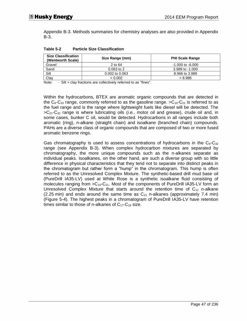
Submitted To 2014 EEM Program Report
Page 47 of 236
Appendix B-3. Methods summaries for chemistry analyses are also provided in Appendix B-3.
Table 5-2 Particle Size Classification
Size Classification (Wentworth Scale)
Size Range (mm) PHI Scale Range
Gravel 2 to 64 -1.000 to -6.000
Sand 0.063 to 2 3.989 to -1.000
Silt 0.002 to 0.063 8.966 to 3.989
Clay < 0.002 < 8.986
Note: - Silt + clay fractions are collectively referred to as "fines".
Within the hydrocarbons, BTEX are aromatic organic compounds that are detected in the C6-C10 range, commonly referred to as the gasoline range. >C10-C21 is referred to as the fuel range and is the range where lightweight fuels like diesel will be detected. The >C21-C32 range is where lubricating oils (i.e., motor oil and grease), crude oil and, in some cases, bunker C oil, would be detected. Hydrocarbons in all ranges include both aromatic (ring), n-alkane (straight chain) and isoalkane (branched chain) compounds. PAHs are a diverse class of organic compounds that are composed of two or more fused aromatic benzene rings.
Gas chromatography is used to assess concentrations of hydrocarbons in the C6-C32 range (see Appendix B-3). When complex hydrocarbon mixtures are separated by chromatography, the more unique compounds such as the n-alkanes separate as individual peaks. Isoalkanes, on the other hand, are such a diverse group with so little difference in physical characteristics that they tend not to separate into distinct peaks in the chromatogram but rather form a “hump” in the chromatogram. This hump is often referred to as the Unresolved Complex Mixture. The synthetic-based drill mud base oil (PureDrill IA35-LV) used at White Rose is a synthetic isoalkane fluid consisting of molecules ranging from >C10-C21. Most of the components of PureDrill IA35-LV form an Unresolved Complex Mixture that starts around the retention time of C11 n-alkane (2.25 min) and ends around the same time as C21 n-alkanes (approximately 7.4 min) (Figure 5-4). The highest peaks in a chromatogram of PureDrill IA35-LV have retention times similar to those of n-alkanes of C17-C18 size.

Submitted To 2014 EEM Program Report
Page 48 of 236
Table 5-3 Sediment Chemistry Variables (2000, 2004, 2005, 2006, 2008, 2010, 2012 and 2014)
Variables Method Laboratory Detection Limit
Units 2000 2004 2005 2006 2008 2010/2012 2014
Hydrocarbons
Benzene Calculated 0.03 0.03 0.03 0.03 0.03 0.03 0.03 mg/kg
Toluene Calculated 0.03 0.03 0.03 0.03 0.03 0.03 0.04 mg/kg
Ethylbenzene Calculated 0.03 0.03 0.03 0.03 0.03 0.03 0.03 mg/kg
Xylenes Calculated 0.05 0.05 0.05 0.05 0.05 0.05 0.05 mg/kg
C6-C10 Calculated 3 3 3 4 3 3 3 mg/kg
>C10-C21 GC/FID 0.3 0.3 0.3 0.3 0.3 0.3 0.3 mg/kg
>C21-C32 GC/FID 0.3 0.3 0.3 0.3 0.3 0.3 0.3 mg/kg
PAHs
1-Chloronaphthalene GC/FID NA 0.05 0.05 0.05 0.05 0.01 0.01 mg/kg
2-Chloronaphthalene GC/FID NA 0.05 0.05 0.05 0.05 0.01 0.01 mg/kg
1-Methylnaphthalene GC/FID 0.05 0.05 0.05 0.05 0.05 0.01 0.01 mg/kg
2-Methylnaphthalene GC/FID 0.05 0.05 0.05 0.05 0.05 0.01 0.01 mg/kg
Acenaphthene GC/FID 0.05 0.05 0.05 0.05 0.05 0.01 0.01 mg/kg
Acenaphthylene GC/FID 0.05 0.05 0.05 0.05 0.05 0.01 0.01 mg/kg
Anthracene GC/FID 0.05 0.05 0.05 0.05 0.05 0.01 0.01 mg/kg
Benz[a]anthracene GC/FID 0.05 0.05 0.05 0.05 0.05 0.01 0.01 mg/kg
Benzo[a]pyrene GC/FID 0.05 0.05 0.05 0.05 0.05 0.01 0.01 mg/kg
Benzo[b]fluoranthene GC/FID 0.05 0.05 0.05 0.05 0.05 0.01 0.01 mg/kg
Benzo[ghi]perylene GC/FID 0.05 0.05 0.05 0.05 0.05 0.01 0.01 mg/kg
Benzo[k]fluoranthene GC/FID 0.05 0.05 0.05 0.05 0.05 0.01 0.01 mg/kg
Chrysene GC/FID 0.05 0.05 0.05 0.05 0.05 0.01 0.01 mg/kg
Dibenz[a,h]anthracene GC/FID 0.05 0.05 0.05 0.05 0.05 0.01 0.01 mg/kg
Fluoranthene GC/FID 0.05 0.05 0.05 0.05 0.05 0.01 0.01 mg/kg
Fluorene GC/FID 0.05 0.05 0.05 0.05 0.05 0.01 0.01 mg/kg
Indeno[1,2,3-cd]pyrene GC/FID 0.05 0.05 0.05 0.05 0.05 0.01 0.01 mg/kg
Naphthalene GC/FID 0.05 0.05 0.05 0.05 0.05 0.01 0.01 mg/kg
Perylene GC/FID 0.05 0.05 0.05 0.05 0.05 0.01 0.01 mg/kg
Phenanthrene GC/FID 0.05 0.05 0.05 0.05 0.05 0.01 0.01 mg/kg
Pyrene GC/FID 0.05 0.05 0.05 0.05 0.05 0.01 0.01 mg/kg
Carbon
Carbon LECO 0.1 0.2 0.2 0.2 0.2 0.2 0.2 g/kg
Organic Carbon LECO 0.1 0.2 0.2 0.2 0.2 0.2 0.2 g/kg
Inorganic Carbon By Diff 0.2 0.3 0.2 0.2 0.2 0.2 0.2 g/kg
Metals
Aluminum ICP-MS 10 10 10 10 10 10 10 mg/kg
Antimony ICP-MS 2 2 2 2 2 2 2 mg/kg
Arsenic ICP-MS 2 2 2 2 2 2 2 mg/kg
Barium ICP-MS 5 5 5 5 5 5 5 mg/kg
Beryllium ICP-MS 5 2 2 2 2 2 2 mg/kg
Cadmium GFAAS 0.05 0.05 0.05 0.05 0.05 0.05 0.05 mg/kg
Chromium ICP-MS 2 2 2 2 2 2 2 mg/kg
Cobalt ICP-MS 1 1 1 1 1 1 1 mg/kg
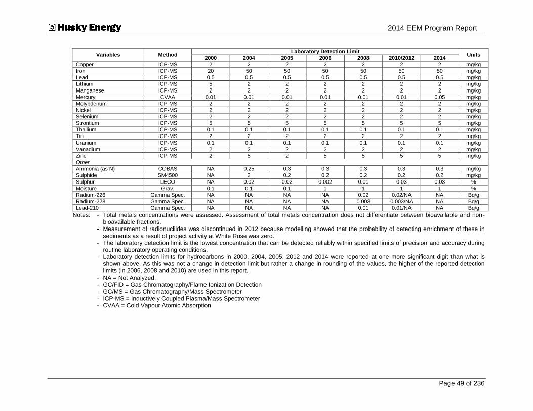
Submitted To 2014 EEM Program Report
Page 49 of 236
Variables Method Laboratory Detection Limit
Units 2000 2004 2005 2006 2008 2010/2012 2014
Copper ICP-MS 2 2 2 2 2 2 2 mg/kg
Iron ICP-MS 20 50 50 50 50 50 50 mg/kg
Lead ICP-MS 0.5 0.5 0.5 0.5 0.5 0.5 0.5 mg/kg
Lithium ICP-MS 5 2 2 2 2 2 2 mg/kg
Manganese ICP-MS 2 2 2 2 2 2 2 mg/kg
Mercury CVAA 0.01 0.01 0.01 0.01 0.01 0.01 0.05 mg/kg
Molybdenum ICP-MS 2 2 2 2 2 2 2 mg/kg
Nickel ICP-MS 2 2 2 2 2 2 2 mg/kg
Selenium ICP-MS 2 2 2 2 2 2 2 mg/kg
Strontium ICP-MS 5 5 5 5 5 5 5 mg/kg
Thallium ICP-MS 0.1 0.1 0.1 0.1 0.1 0.1 0.1 mg/kg
Tin ICP-MS 2 2 2 2 2 2 2 mg/kg
Uranium ICP-MS 0.1 0.1 0.1 0.1 0.1 0.1 0.1 mg/kg
Vanadium ICP-MS 2 2 2 2 2 2 2 mg/kg
Zinc ICP-MS 2 5 2 5 5 5 5 mg/kg
Other
Ammonia (as N) COBAS NA 0.25 0.3 0.3 0.3 0.3 0.3 mg/kg
Sulphide SM4500 NA 2 0.2 0.2 0.2 0.2 0.2 mg/kg
Sulphur LECO NA 0.02 0.02 0.002 0.01 0.03 0.03 %
Moisture Grav. 0.1 0.1 0.1 1 1 1 1 %
Radium-226 Gamma Spec. NA NA NA NA 0.02 0.02/NA NA Bq/g
Radium-228 Gamma Spec. NA NA NA NA 0.003 0.003/NA NA Bq/g
Lead-210 Gamma Spec. NA NA NA NA 0.01 0.01/NA NA Bq/g
Notes: - Total metals concentrations were assessed. Assessment of total metals concentration does not differentiate between bioavailable and non-bioavailable fractions.
- Measurement of radionucliides was discontinued in 2012 because modelling showed that the probability of detecting enrichment of these in sediments as a result of project activity at White Rose was zero.
- The laboratory detection limit is the lowest concentration that can be detected reliably within specified limits of precision and accuracy during routine laboratory operating conditions.
- Laboratory detection limits for hydrocarbons in 2000, 2004, 2005, 2012 and 2014 were reported at one more significant digit than what is shown above. As this was not a change in detection limit but rather a change in rounding of the values, the higher of the reported detection limits (in 2006, 2008 and 2010) are used in this report.
- NA = Not Analyzed. - GC/FID = Gas Chromatography/Flame Ionization Detection - GC/MS = Gas Chromatography/Mass Spectrometer - ICP-MS = Inductively Coupled Plasma/Mass Spectrometer - CVAA = Cold Vapour Atomic Absorption

Submitted To 2014 EEM Program Report
Page 50 of 236
Figure 5-4 Gas Chromatogram Trace for PureDrill IA35-LV
5.1.2.2 Toxicity
Analytical Methods
Sediment toxicity analyses were conducted at petroforma inc. in St. John’s, Newfoundland and Labrador. Sediment samples were examined using the amphipod survival bioassay and the bacterial luminescence assay. Both bioassays used whole sediment as the test matrix. Tests with lethal endpoints, in this case, amphipod survival, measure survival over a defined exposure period. Tests with sublethal endpoints measure physiological functions of the test organism, such as metabolism, fertilization and growth, over a defined exposure period. Bacterial luminescence, in this case, was used as a measure of metabolism. Tests that rely on sublethal endpoints are a potential gauge of long-term effects.
Amphipod survival tests were conducted according to Environment Canada (1998) protocols using the marine amphipod Rhepoxynius abronius obtained from West Beach, Whidbey Island, Washington State (USA). R. abronius is a standard and widely used test species. Although it is not native to the East Coast of Canada, related species in the family Phoxocephalidae are among the more abundant amphipods in White Rose benthic invertebrate communities. Tests involved five replicate 1-L test chambers with approximately 2 cm of sediment and approximately 800 mL of overlying water (Figure. 5-5).

Submitted To 2014 EEM Program Report
Page 51 of 236
Figure 5-5 Amphipod Survival Test
Each test container was set up with 20 test organisms and maintained for 10 days under appropriate test conditions, after which survival was recorded. An additional test container was used for water quality monitoring only. Negative control sediment was tested concurrently, since negative controls provide a baseline response against which test organisms can be compared. Negative control sediment, known to support a viable population, was obtained from the collection site for the test organisms. A positive (toxic) control in aqueous solution was tested for each batch of test organisms received. Positive controls provide a measure of precision for a particular test, monitor seasonal and batch sensitivity to a specific toxicant. Ancillary testing of total ammonia and sulphides in overlying water was conducted by an ammonia ion selective probe and colorimetric determination, respectively.
Amphipod toxicity tests were initiated two to six days outside the six weeks holding period recommended by Environment Canada (1998) because of amphipod unavailability (amphipod collection delays due to inclement weather).
Submitted To 2014 EEM Program Report
Page 52 of 236
The bacterial luminescence test was performed with Vibrio fishcheri. This bacterium emits light as a result of normal metabolic activities. This assay was conducted according to the Environment Canada (2002) Reference Method using the large volume solid phase assay. Analysis was conducted on a Model 500 Photometer with a computer interface. A geometric series of sediment concentrations was set up using Azur solid phase diluent. The actual number of concentrations was dependent on the degree of reduction in bioluminescence observed. Negative (clean) and positive (toxic) controls were run concurrently with the test samples. Reduction of light after 15 minutes was used to measure toxicity. Data interpretation for 2004, 2005, 2006, 2008, 2010, 2012 and 2014 was conducted as outlined in Environment Canada’s (2002) Reference Method. Data from the 2000 (baseline) program were reexamined using the criteria outlined in Environment Canada (2002) because analyses in 2000 were conducted using earlier Environment Canada guidelines (small volume solid phase assay; Environment Canada 1992). Reinterpretation of 2000 data using Environment Canada (2002) did not alter any of the 2000 interpretations.
All bacterial luminescence tests were initiated within six weeks of sample collection, as recommended by Environment Canada (2002).
Results Interpretation
The statistical endpoint for the amphipod toxicity test is the determination of whether the biological endpoint (percent survival) differs statistically from the control or reference sample. This endpoint was calculated using the Dunnett’s Multiple Comparison Test using the CETIS computer program (©2001-2010 Tidepool Scientific, LLC). The statistical endpoint for the bacterial luminescence toxicity test is the determination of whether the biological endpoint (bioluminescence) for the sample is significantly different from the negative control (0%), calculated as the IC50
7 value.
petroforma inc. conducted amphipod toxicity tests using two separate reference samples: negative control sediment that comes from the source site for the amphipods (B6178-09); and a site reference that is a composite of four reference stations (stations 4, 12, 19, 27) and is called “WRRS (4, 12, 19, 27). Using two reference samples to define toxicity reduces an already very low risk of false positives. Sample toxicity was assessed using standard toxicity testing statistical programs. The amphipod survival test results for sediments were considered toxic if the survival was reduced by more than 30% reduction as compared to the negative control sediment; and the result was statistically significantly different from survival in the negative control sediment. Amphipod survival was also compared to White Rose Reference Station sediment (WRRS; stations 4, 12, 19 and 27). For this EEM program, the amphipod survival test results for sediments were considered toxic if survival was reduced by more than 20% as compared to WRRS sample and the result was statistically significantly different from survival in the WRRS sample.
The Reference Method for Determining the Toxicity of Sediment Using Luminescent Bacteria in a Solid-Phase Test (Environment Canada 2002) was also used to assess sediments. Sediments with levels of silt/clay greater than 20% are considered to be toxic if the IC50 is less than 1,000 mg/L as dry solids.
7 An IC50 (50% inhibitory concentration) is the concentration of a substance that produces 50% of the
maximum possible inhibitory response to that substance.
Submitted To 2014 EEM Program Report
Page 53 of 236
For any test sediment from a particular station that is comprised of less than 20% fines and that has an IC50 of ≥1,000 mg/L (dry weight), the IC50 of this sediment must be compared against a sample of “clean” reference sediment or negative control sediment (artificial or natural) with a percent fines content that does not differ by more than 30% from that of the test sediment. Based on this comparison, the test sediment is judged to have failed the sediment toxicity test if, and only if, both of the following two conditions apply:
1. its IC50 is more than 50% lower than that determined for the sample reference sediment or negative control sediment; and
2. the IC50s for the test sediment and reference sediment or negative control sediment differ significantly.
5.1.2.3 Benthic Community Structure
All 2014 benthic invertebrate samples were provided whole to Arenicola Marine Limited (Wolfville, Nova Scotia). Individual core samples were processed separately but data were pooled for data analysis (see Section 5.1.4).
Sandy samples were washed through a 0.5 mm sieve. Samples with larger proportions of coarse material (gravel and shell) were elutriated and sieved by directing a high volume (1 L/s) flow of freshwater into the sample, tilting the sample bucket and catching the overflow on the sieve. This washing removed the silt/clay and finer sand fractions from the samples. The procedure was adjusted to leave coarser sediment fractions in the pail. The flow suspended the less dense organisms (e.g., polychaetes) and separated small gastropods and clams which, with a suitable balance of flow in and out of the bucket, could be separated as well. Elutriation was continued until the water leaving the pail was free of organisms and when no additional heavier organisms could be seen after close examination of the sediment. Usually, larger organisms such as scallops and propeller clams were separated manually as they were found. Barnacles and sponges were scraped off rocks. With coarser sediments such as gravels, which were occasionally encountered, a 1.2 cm mesh in combination with the 0.5 mm screen was used to aid in separating the organisms. Organisms were placed in 70% alcohol after sieving.
Samples were sorted under a stereomicroscope at 6.4x magnification, with a final scan at 16x. After sorting, substrate from 10% of samples was reexamined by a different sorter to determine sorting efficiency. Efficiency levels ranging from 98 to 100% were achieved (i.e., the first sorter recovered 98 to 100%% of the organisms recovered by both sorters combined). Wet weight biomass (g/sample) was estimated by weighing animals to the nearest milligram at the time of sorting after blotting to remove surface water. None of the samples were subsampled.
Organisms were identified to the lowest practical taxonomic level, typically to species, using conventional literature for the groups involved (Appendix B-4). All organisms were identified by Patricia Pocklington, a specialist in marine benthic invertebrate taxonomy.
Benthic invertebrate samples for 2004, 2005, 2006, 2008, 2010 and 2012 were also processed by Arenicola Marine Limited. Benthic invertebrate samples from 2000 were processed by Pat Stewart of Envirosphere Limited. Methods and the level of taxonomy

Submitted To 2014 EEM Program Report
Page 54 of 236
were similar to those used for the 2004 to 2014 samples (see Husky Energy 2001 for details).
5.1.3 Data Quality Control
Analytical labs used for the sediment program included Maxxam Analytics (particle size analyses and sediment chemistry analyses (extractable petroleum hydrocarbons, metals)) and petroforma inc. (sediment chemistry analyses (volatile petroleum hydrocarbons, PAH, moisture, mercury, sulphides, sulphur, TIC/TOC/total carbon) and sediment toxicity analyses). Quality assurance samples were collected for the water and sediment chemistry analyses, as well as field blanks, and the laboratories conducted their own lab duplicates during the analyses. Results, including quality assurance and quality control samples, are provided in Appendices B-1 (particle size analyses) and B-2 (chemistry analyses). In general, the overall quality control for the analyses met acceptability criteria.
As there were substantial differences in (TOC) values in 2014 compared to previous years, petroforma inc. conducted a review of the QC, data and the method protocol. Prior to sample preparation, samples were kept frozen in their containers. Each sample was treated in the same fashion during sample preparation for the test. While not in direct testing, the prepped samples were kept isolated from the general lab area to avoid contamination with organics wherever possible until the time of analysis. petroforma inc. performed duplicate tests every 20 samples to ensure repeatability of the instrument. Daily quality control calibration checks were performed, and all were acceptable. In instances where the signal was high (i.e., the total carbon amount was high), the sample masses were reduced and the result verified. The sample analysis was repeated on a smaller sample size (for example, this occurred for stations S4 and S1, which had the highest total carbon content of the set), and since the high total carbon amount observed was duplicated on a second aliquot of sample, it was therefore concluded that the high total carbon result for that sample was a real response (i.e., the sample aliquot used in the analysis was not contaminated). Since the QC and other duplicate sample results were satisfactory, this also supported the conclusion that the result was real. Based on petroforma inc.’s review, the results appear valid.
5.1.4 Data Analysis
The White Rose Sediment Quality survey is based on a gradient design, with sampling locations radiating out from the general operations area defined by the Northern, Southern, Central, North Amethyst and SWRX Drill Centres. Effects during development drilling periods (since operations began; from 2004 to present) at White Rose have historically been most evident close to active drill centres and have decreased with distance away from them. The general approach for the examination of the Sediment Quality data was to confirm the presence of spatial patterns (i.e., changes in response variables with distance from active drill centres) that were consistent with development drilling effects and to identify the potential zone of influence8 for sediment chemistry. Drill centres were considered active if any drilling had occurred there in the past.
8 The zone of influence has been defined as the zone where physical and chemical alterations might occur (see Section 1).

Submitted To 2014 EEM Program Report
Page 55 of 236
As indicated in Husky’s response to regulator comments on the 2008 EEM program (see Appendix A-1 in the 2010 EEM Program Report, Husky Energy 2011), the EEM reports now rely on both statistical analysis and visual display of information in order to assess effects. Occurrence above or below the range of values observed during baseline sampling (2000) is used to assess effects from individual drill centres.
Station 31 was excluded from all analyses of physical and chemical characteristics of sediments in 2008, 2010, 2012 and 2014 because it is a clear outlier in terms of chemistry (hydrocarbons and barium in particular). Station 31 is located 4.2 km from the nearest development drill centre but the station is located near the site of a delineation well drilled in 2007. Station 31 was included in distance trend analyses in 2014 for laboratory toxicity test results and benthic indices, because it was not an outlier for biological measures.
5.1.4.1 Physical and Chemical Characteristics
Data were first screened to identify and exclude variables that frequently occurred below detectable concentrations. The variables selected for detailed analysis in 2014 included >C10-C12 hydrocarbons, barium, sediment particle size (% fines and % gravel), concentrations of TOC, ammonia, sulphide9, sulphur, redox potential and a summary measure of concentration of metals other than barium (derived from a principal component analysis (PCA) of metals data). Also, because the metals PCA indicated that lead and strontium behaved differently from other metals, these two metals were examined separately. The rationale for selecting these variables is provided below.
Synthetic-based drill muds have elevated concentrations of >C10-C21 hydrocarbons. Barium, as barium sulphate (barite), can be a constituent of both water-based and synthetic-base drill muds. Sediment particle size (particularly % fines) and TOC content could be altered by drilling activity. Water-based and synthetic-based muds and associated drill cuttings are finer than the predominantly sand substrate on the Grand Banks, and synthetic-based muds have a higher organic carbon content than natural substrates.
Percent gravel has previously been correlated with indices of benthic community structure. As in previous years, percent sand was not examined because it is strongly negatively correlated with percent gravel and, generally speaking, percent fines constitute a very small fraction of sediment particle size.
Sulphur, as sulphate in barite, is also an important constituent of drill muds. Ammonia and sulphide levels are typically high, and redox levels are low, in sediments where decomposition or degradation of natural or synthetic organic matter is extensive. Ammonia and sulphides, as well as particle size, are also important confounding factors that need to be considered in the interpretation of toxicity test results (Tay et al. 1998). Metals other than barium can also be enriched in drill cuttings, albeit to a lesser extent.
Five statistical tools were used to explore the spatial variations of these selected variables as they might relate to drilling. These tools are described below.
9 Sulphide results were dominated by data below laboratory detection limits across all years; however, all available sulphide data were used in statistical analyses to aid in interpretation of data from 2006, 2008 and 2014 that had the majority of results above laboratory detection limits.

Submitted To 2014 EEM Program Report
Page 56 of 236
Spearman rank correlation (Tool 1) was used to statistically test for associations between distance from the nearest active drill centre and concentration of the subset of variables selected for detailed analysis.
Threshold models (Tool 2) were constructed in order to estimate the spatial extent (threshold distance) of influence of active drill centres, overall, on concentrations of substances in sediments for those variables that were demonstrated with Spearman rank correlations to be significantly correlated with distance from the nearest active drill centre.
The third tool (Tool 3) involved visual inspection of response variable data from 2000 to present. Scatterplots of concentration (or percent as appropriate) in relation to distance from the nearest active drill centre were produced in order to visualize the nature of the relationship with distance.
Maps (Tool 4) indicating concentrations within and exceeding the variability observed in baseline (2000), or background variability (stations with a distance to the nearest drill centre greater than 10 km) if baseline data were unavailable, were generated to visually assess the effects of individual drill centres on variables that were demonstrated with Spearman rank correlations to be significantly correlated with distance from the nearest active drill centre.
Repeated-measures regression (Tool 5) was used to test for spatial and temporal variation for barium and >C10-C21 hydrocarbons, and other variables brought forward for detailed analysis, at those stations that have been repeatedly sampled since baseline. The repeated-measures regression method was used to determine if there were changes over time both in terms of changes in mean concentration across all sampling locations (i.e., an increase in or decrease in concentration that is similar across all stations), or a change in the nature of the relationship between distance to the nearest active drill centre (i.e., Min D) and concentration (i.e., the slope of the relationship may get steeper over time, indicating an increase in concentrations adjacent to active drill centres). The repeated-measures regression was carried out with the 35 stations that were repeatedly sampled in baseline and EEM years (excluding station 31 because it was an outlier, see Section 5.1.3). Repeated-measured regression was complemented by Spearman rank correlations computed between response variables and Min D, by year, using all stations where sediment triad data were available. The Spearman rank correlations were based on more stations than was the repeated-measures regression, and so the results of each analysis did at times indicate different trends over time. However, plots of the Spearman rank correlations assisted in the interpretation of the repeated-measures regression analysis.
All statistical methods pertaining to sediment quality are described in greater detail in Appendix B-5.
5.1.4.2 Toxicity
In 2014 and in previous years, no analyses of results for bacterial luminescence toxicity tests were conducted because there were very few samples which were determined to be toxic using this test. A single toxic sample was noted in 2010. Three samples were toxic in 2014. No toxic response was noted in any other year.

Submitted To 2014 EEM Program Report
Page 57 of 236
The evidence that amphipod survival was influenced by drilling was tested using Spearman rank correlation of survival and distance to the nearest active drill centre.
5.1.4.3 Benthic Community Composition
In 2014, benthic community composition analysis focused on three summary indices:
total abundance (number of organisms per m²);
biomass (wet weight of organisms per m²); and
taxonomic richness (number of families per station).
Abundances of four taxa were also analyzed in some detail. These analyses were secondary to analyses of indices of benthic community composition and were performed to provide insight on the more general indices. Taxa examined were:
Paraonidae (Polychaeta);
Spionidae (Polychaeta);
Tellinidae (Bivalvia); and
Amphipoda.
Paraonidae, Spionidae and Tellinidae were the three most abundant taxa. Although Amphipoda were relatively rare, they were included in analyses of individual taxa because they are generally considered sensitive and were also reduced in abundance near active drill centres and at relatively high >C10-C21 hydrocarbon concentrations in past years (Husky Energy 2011).
As with the sediment chemistry and amphipod toxicity results, the objective of the detailed analysis of the benthic community data was to test for evidence effects from active drill centres. Five statistical tools were used to explore the spatial variations of the selected indices of benthic community composition: rank regression (Tool 1), threshold models (Tool 2), graphical display of data (Tool 3), maps (Tool 4) and repeated-measures regression (Tool 5). For individual taxa, only those taxa that showed significant correlations with distance from active drill centres were examined using maps.
All of these methods are described in greater detail in Appendix B-5.
5.2 Results
5.2.1 Physical and Chemical Characteristics
Appendix B-3 provides summary statistics at Sediment Quality Triad stations for sediment physical and chemical characteristics occurring at or above the laboratory detection limit in 2000, 2004, 2005, 2006, 2008, 2010, 2012 and 2014. All variables measured on sediment are provided above in Table 5-3. Toluene was detected at levels close to the laboratory detection limit at one station in 2005 and was not detected in other years. >C10-C21 and >C21-C32 hydrocarbons have been detected in sediments since 2004,
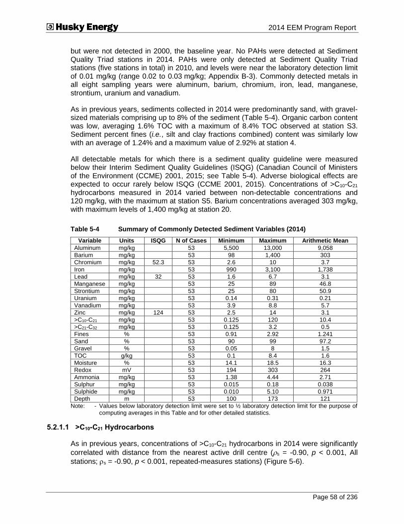
Submitted To 2014 EEM Program Report
Page 58 of 236
but were not detected in 2000, the baseline year. No PAHs were detected at Sediment Quality Triad stations in 2014. PAHs were only detected at Sediment Quality Triad stations (five stations in total) in 2010, and levels were near the laboratory detection limit of 0.01 mg/kg (range 0.02 to 0.03 mg/kg; Appendix B-3). Commonly detected metals in all eight sampling years were aluminum, barium, chromium, iron, lead, manganese, strontium, uranium and vanadium.
As in previous years, sediments collected in 2014 were predominantly sand, with gravel-sized materials comprising up to 8% of the sediment (Table 5-4). Organic carbon content was low, averaging 1.6% TOC with a maximum of 8.4% TOC observed at station S3. Sediment percent fines (i.e., silt and clay fractions combined) content was similarly low with an average of 1.24% and a maximum value of 2.92% at station 4.
All detectable metals for which there is a sediment quality guideline were measured below their Interim Sediment Quality Guidelines (ISQG) (Canadian Council of Ministers of the Environment (CCME) 2001, 2015; see Table 5-4). Adverse biological effects are expected to occur rarely below ISQG (CCME 2001, 2015). Concentrations of >C10-C21
hydrocarbons measured in 2014 varied between non-detectable concentrations and 120 mg/kg, with the maximum at station S5. Barium concentrations averaged 303 mg/kg, with maximum levels of 1,400 mg/kg at station 20.
Table 5-4 Summary of Commonly Detected Sediment Variables (2014)
Variable Units ISQG N of Cases Minimum Maximum Arithmetic Mean
Aluminum mg/kg 53 5,500 13,000 9,058
Barium mg/kg 53 98 1,400 303
Chromium mg/kg 52.3 53 2.6 10 3.7
Iron mg/kg 53 990 3,100 1,738
Lead mg/kg 32 53 1.6 6.7 3.1
Manganese mg/kg 53 25 89 46.8
Strontium mg/kg 53 25 80 50.9
Uranium mg/kg 53 0.14 0.31 0.21
Vanadium mg/kg 53 3.9 8.8 5.7
Zinc mg/kg 124 53 2.5 14 3.1
>C10-C21 mg/kg 53 0.125 120 10.4
>C21-C32 mg/kg 53 0.125 3.2 0.5
Fines % 53 0.91 2.92 1.241
Sand % 53 90 99 97.2
Gravel % 53 0.05 8 1.5
TOC g/kg 53 0.1 8.4 1.6
Moisture % 53 14.1 18.5 16.3
Redox mV 53 194 303 264
Ammonia mg/kg 53 1.38 4.44 2.71
Sulphur mg/kg 53 0.015 0.18 0.038
Sulphide mg/kg
53 0.010 5.10 0.971
Depth m 53 100 173 121
Note: - Values below laboratory detection limit were set to ½ laboratory detection limit for the purpose of computing averages in this Table and for other detailed statistics.
5.2.1.1 >C10-C21 Hydrocarbons
As in previous years, concentrations of >C10-C21 hydrocarbons in 2014 were significantly
correlated with distance from the nearest active drill centre (s = -0.90, p < 0.001, All
stations; s = -0.90, p < 0.001, repeated-measures stations) (Figure 5-6).

Submitted To 2014 EEM Program Report
Page 59 of 236
RM Stations
All Stations
2000 2002 2004 2006 2008 2010 2012 2014
Year
-1.0
-0.5
0.0
0.5
1.0
Sp
earm
an
Ran
k >C10-C21 Hydrocarbons
Figure 5-6 Spearman Rank Correlations with Distance from the Nearest Active Drill Centre for >C10-C21 Hydrocarbons
Notes: Station 31 was excluded. n = 52 for All Stations. n = 35 for Repeated-Measures (RM) Stations. Dotted lines indicate rank correlations of |0.3|, which were generally significant at p < 0.01,
depending on sample size in the given year; however, significance from specific statistical tests reported in text.
A threshold model describing the relationship between concentrations of >C10-C21 hydrocarbons and distance from the nearest active drill centre was significant (p < 0.001). In 2014, the threshold distance was estimated to be 5.8 km (Table 5-5). Figure 5-7 provides a graphical representation of threshold models.
Table 5-5 Results of Threshold Regressions on Distance from the Nearest Active Drill Centre for >C10-C21 Hydrocarbons
Year Threshold Distance (km)
2004 6.3 (4.1, 9.7)
2005 8.9 (4.9, 16)
2006 5.9 (4.2, 8.5)
2008 10.4 (5.2, 20.9)
2010 3.6 (2.9, 4.4)
2012 3.6 (2.6, 4.8)
2014 5.8 (3.5, 9.5)
Notes: - 95% confidence limits are provided in brackets. - n = 52 in 2014 with station 31 excluded.
As indicated in Figure 5-7, no hydrocarbons were detected in White Rose sediments during baseline sampling. As in previous EEM years, >C10-C21 hydrocarbon concentrations were enriched around active drill centres in 2014 (Figure 5-8). >C10-C21 hydrocarbons were also still enriched at station 31, located near the site of a delineation well drilled in 2007 (Figure 5-8).

Submitted To 2014 EEM Program Report
Page 60 of 236
Station 31
Station 31
Station 31
Station 31
0.1 1 10 100
Min D (km)
0.1
1
10
100
1000
>C
10 -C
21(m
g/k
g)
2000
0.1 1 10 100
0.1
1
10
100
2004
1 10 100
Min D (km)
1000
>C
10 -C
21(m
g/k
g)
0.1 1 10 100
0.1
1
10
100
1000
2005
1 10 100
Min D (km)
>C
10 -C
21(m
g/k
g)
0.1 1 10 100
0.1
1
10
100
1000
2006
1 10 100
Min D (km)
>C
10 -C
21(m
g/k
g)
1 10 100
10
100
1000
0.1 1 10 100
Min D (km)
1
10
>C
10 -C
21(m
g/k
g)
1 10 100
Min D (km)
1
10
21
1 10 100
Min D (km)
0.1
1
10
21
0.1 1 10 100
0.1
10
100
1000
1 10 100
Min D (km)
1
10
>C
10
21(m
g/k
g)
2010
1 10 100
Min D (km)
1
10 -C
21
1 10 100
Min D (km)
1 10 100
0.1
1
10
100
1000
2012
0.1 1 10 100
Min D (km)
>C
10 -C
21
1 10 100
Min D (km)
21
1 10 100
Min D (km)
(mg/k
g)
0.1 1 10 100
10
100
1000
2014
0.1 1 10 100
Min D (km)
0.1
1
10
>C
10 -C
21(m
g/k
g)
1 10 100
Min D (km)
1
1 10 100
Min D (km)
1
2008
Figure 5-7 Variations in >C10-C21 Concentrations with Distance from the Nearest Active Drill Centre (all Years)
Notes: Min D = distance (km) to the nearest active drill centre, except in 2000 (baseline), where Min D is distance to the nearest future drill centre. The ½ of the detection limit is indicated in each graph by a
horizontal dotted line (0.15 mg/kg), to indicate the levels observed in the baseline year (2000).
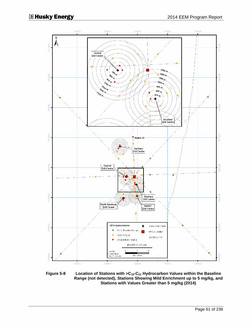
Submitted To 2014 EEM Program Report
Page 61 of 236
Figure 5-8 Location of Stations with >C10-C21 Hydrocarbon Values within the Baseline Range (not detected), Stations Showing Mild Enrichment up to 5 mg/kg, and
Stations with Values Greater than 5 mg/kg (2014)

Submitted To 2014 EEM Program Report
Page 62 of 236
Repeated-measures regression indicated no change over time in the relationship between distance and concentrations of >C10-C21 hydrocarbons for repeated-measures stations (p = 0.502; Table 5-6), and no changes in area-wide concentrations over time (p = 0.642). This conclusion applies to the time period from 2004 to present. (i.e., EEM years). Concentrations of >C10-C21 hydrocarbons were non-detectable in 2000, and generally have been at detectable concentrations since 2004 (Figures 5-7 and 5-9).
Table 5-6 Repeated-measures Regression Testing for Changes in >C10-C21 Concentrations over Time
Trend Over Time Before to After
Slope Mean Slope Mean
0.502 0.642 NA NA
Notes: - Values are probabilities. - n = 35 with station 31 excluded.
- The trend over Time contrast tests for trends over time since operations began (i.e., from 2004 to 2014).
- The Before to After contrast tests for differences between year 2000 (baseline) and the mean in the period including 2004 to 2012. The Before to After contrast cannot be performed for >C10-C21 hydrocarbons since all concentrations were below detection limit during baseline.
2000 2004 2005 2006 2008 2010 2012 2014
Year
0.1
1
10
100
1000
>C
10-C
21
(mg
/kg
)
Figure 5-9 Dot Density Plot of >C10-C21 Hydrocarbon Values by Year
Note: The horizontal dotted line indicates ½ the detection limit (0.15 mg/kg), to indicate the levels observed in the baseline year (2000).
5.2.1.2 Barium
Like >C10-C21 hydrocarbons, barium produced a significant Spearman rank correlation
with distance to active drill centres in 2014 (s = -0.59, p < 0.001, All stations; s = -0.60, p < 0.001, repeated-measures stations), as in previous years (Figure 5-10).

Submitted To 2014 EEM Program Report
Page 63 of 236
RM Stations
All StationsBarium
2000 2002 2004 2006 2008 2010 2012 2014
Year
-1.0
-0.5
0.0
0.5
1.0
Sp
earm
an
Ran
k
Figure 5-10 Spearman Rank Correlations with Distance from the Nearest Active Drill Centre for Barium
Notes: Station 31 was excluded. n = 52 for All Stations. n = 35 for Repeated-Measures (RM) Stations. Dotted lines indicate rank correlations of |0.3|, which were generally significant at p < 0.01, depending on
sample size in the given year; however, significance from specific statistical tests reported in text.
The threshold model in 2014 was again significant (p < 0.001). The estimated threshold distance in 2014 was 1 km (Table 5-7). Figure 5-11 provides a graphical representation of threshold models.
Table 5-7 Results of Threshold Regressions on Distance from the Nearest Active Drill Centre for Barium
Year Threshold Distance (km)
2004 2.4 (1.6 to 3.5)
2005 3.6 (2.1 to 6.2)
2006 1.9 (1.4 to 2.6)
2008 2.4 (1.5 to 3.8)
2010 2.0 (1.6 to 2.5)
2012 1.0 (0.8, 1.2)
2014 1.0 (0.8, 1.4)
Notes: - 95% confidence limits are provided in brackets. - n = 52 in 2014 with station 31 excluded.
As indicated in Figure 5-11, the “normal range” of variation for barium concentration in sediments across the sampling area was computed from the 2000 baseline data. Values in 2000 ranged between 120 and 210 mg/kg. The value 202 mg/kg was used as a “benchmark” against which to judge spatial variation in the sampling area in Figures 5-11 and 5-12. The steepest threshold regression slopes were noted between 2006 and 2012, with the slope for 2014 noticeably reduced (Figure 5-11).
Barium was enriched to levels exceeding 300 mg/kg around the Central, North Amethyst Southern and Northern Drill Centres (Figure 5-12). Barium was also enriched at station 31, located near the site of a delineation well drilled in 2007 (Figure 5-12). Barium was not enriched near the SWRX Drill Centre (Figure 5-12).

Submitted To 2014 EEM Program Report
Page 64 of 236
0.1 1 10 100
Min D (km)
100
1000
Barium
(m
g/k
g)
2000
0.1 1 10 100
100
2004
1 10 100
Min D (km)
1000
Barium
(m
g/k
g)
1 10 100
100
1000
2005
0.1 1 10 100
Min D (km)
Barium
(m
g/k
g)
0.1 1 10 100
1000
2006
1 10 100
Min D (km)
100
Barium
(m
g/k
g)
0.1 1 10 100
100
1000
0.1 1 10 100
Min D (km)1 10 100
Min D (km)1 10 100
Min D (km)
Barium
(m
g/k
g)
0.1 1 10 100
100
1000
2010
0.1 1 10 100
Min D (km)B
arium
(m
g/k
g)
1 10 100
Min D (km)1 10 100
Min D (km)
1 10 100
100
1000
2012
1 10 100
Min D (km)0.1 1 10 100
Min D (km)
Barium
(m
g/k
g)
0.1 1 10 100
Min D (km)
0.1 1 10 100
100
1000
2014
0.1 1 10 100
Min D (km)1 10 100
Min D (km)1 10 100
Min D (km)
Barium
(m
g/k
g)
2008Station 31
Station 31
Station 31
Station 31
Figure 5-11 Variations in Barium Concentrations with Distance from the Nearest Active
Drill Centre (all Years)
Notes: Min D = distance (km) to the nearest active drill centre, except in 2000 (baseline), where Min D is distance to the nearest future drill centre. A concentration of 202 mg/kg is indicated in each graph by a
horizontal line, based on the mean values + 2 SDs from 2000 (baseline).

Submitted To 2014 EEM Program Report
Page 65 of 236
Figure 5-12 Location of Stations with Barium Levels Within the Baseline Range, Stations Showing Mild Enrichment up to 300 mg/kg, and Stations with
Values Greater than 300 mg/kg (2014)

Submitted To 2014 EEM Program Report
Page 66 of 236
Repeated-measures regression indicated that there was no significant linear trend over time in the slope of the relationship between barium concentration and distance to the nearest active drill centre from 2004 to 2014 for repeated-measures stations (p = 0.119; Table 5-8). However, there was a significant trend over time in the average barium concentration (p = 0.015), with barium generally increasing over time in EEM years (Figure 5-13). Slopes differed from before to after drilling operations began (p < 0.001) (Figure 5-1010; Table 5-8). Concentrations of barium in year 2000 averaged 168 mg/kg, with no significant correlation noted between barium concentrations and distance from drill centres (e.g., Figure 5-10). Conversely, distance correlations have been strong for barium since drilling began. Overall average barium concentrations have been higher since drilling operations began (p < 0.001; Table 5-8).
Table 5-8 Repeated-measures Regression Testing for Changes in Barium Concentrations over Time
Trend over Time Before to After
Slope Mean Slope Mean
0.119 0.015 <0.001 <0.001
Notes: - Values are probabilities. - n = 35 with station 31 excluded. - The trend over Time contrast tests for trends over time since operations began (i.e., from 2004 to
2014). - The Before to After contrast tests for differences between year 2000 (baseline) and the mean in
the period including 2004 to 2014.
2000 2004 2005 2006 2008 2010 2012 2014
Year
100
1000
Bari
um
(m
g/k
g)
Figure 5-13 Dot Density Plot of Barium Values by Year
Note: A concentration of 202 mg/kg is indicated in each graph by a horizontal line, as based on the mean values + 2 SDs using data from the baseline year (2000).
10 Although slopes from Spearman rank correlations (Figure 5-10 and other similar figures) are not the same as slopes from repeated-measures regression (the former is non-parametric and includes all stations, the latter is parametric and includes only repeated-measures stations), Figure 5-10 (and other similar figures) can often be used to better understand repeated-measures regression results.
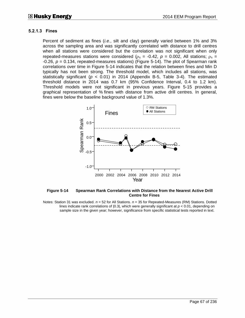
Submitted To 2014 EEM Program Report
Page 67 of 236
5.2.1.3 Fines
Percent of sediment as fines (i.e., silt and clay) generally varied between 1% and 3% across the sampling area and was significantly correlated with distance to drill centres when all stations were considered but the correlation was not significant when only
repeated-measures stations were considered (s = -0.42, p = 0.002, All stations; s = -0.26, p = 0.134, repeated-measures stations) (Figure 5-14). The plot of Spearman rank correlations over time in Figure 5-14 indicates that the relation between fines and Min D typically has not been strong. The threshold model, which includes all stations, was statistically significant (p < 0.01) in 2014 (Appendix B-5, Table 3-4). The estimated threshold distance in 2014 was 0.7 km (95% Confidence Interval, 0.4 to 1.2 km). Threshold models were not significant in previous years. Figure 5-15 provides a graphical representation of % fines with distance from active drill centres. In general, fines were below the baseline background value of 1.3%.
RM Stations
All StationsFines
2000 2002 2004 2006 2008 2010 2012 2014
Year
-1.0
-0.5
0.0
0.5
1.0
Sp
earm
an
Ran
k
Figure 5-14 Spearman Rank Correlations with Distance from the Nearest Active Drill Centre for Fines
Notes: Station 31 was excluded. n = 52 for All Stations. n = 35 for Repeated-Measures (RM) Stations. Dotted lines indicate rank correlations of |0.3|, which were generally significant at p < 0.01, depending on sample size in the given year; however, significance from specific statistical tests reported in text.

Submitted To 2014 EEM Program Report
Page 68 of 236
0.1 1.0 10.0 100.0
Min D (km)
0
2
4
6
8
10
Fin
es (
%)
2000
0.1 1.0 10.0 100.0
Min D (km)
0
2
4
6
8
10
Fin
es (
%)
2004
0.1 1.0 10.0 100.0
Min D (km)
0
2
4
6
8
10
Fin
es (
%)
2005
0.1 1.0 10.0 100.0
Min D (km)
0
2
4
6
8
10
Fin
es (
%)
2006
0.1 1.0 10.0 100.0
Min D (km)
0
2
4
6
8
10
Fin
es (
%)
2008
0.1 1.0 10.0 100.0
Min D (km)
0
2
4
6
8
10
Fin
es (
%)
2010
0.1 1.0 10.0 100.0
Min D (km)
0
2
4
6
8
10
Fin
es (
%)
2012
0.1 1.0 10.0 100.0
10
2014
Min D (km)
0
2
4
6
8
Fin
es (
%)
Figure 5-15 Variations in Percent Fines with Distance from the Nearest Active Drill Centre (all Years)
Notes: Min D = distance (km) to the nearest active drill centre, except in 2000 (baseline), where Min D is distance to the nearest future drill centre. A concentration of 1.3% is indicated in each graph by a horizontal
line, based on the mean values + 2 SDs in 2000 (baseline).
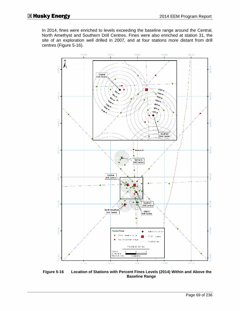
Submitted To 2014 EEM Program Report
Page 69 of 236
In 2014, fines were enriched to levels exceeding the baseline range around the Central, North Amethyst and Southern Drill Centres. Fines were also enriched at station 31, the site of an exploration well drilled in 2007, and at four stations more distant from drill centres (Figure 5-16).
Figure 5-16 Location of Stations with Percent Fines Levels (2014) Within and Above the Baseline Range

Submitted To 2014 EEM Program Report
Page 70 of 236
Repeated-measures regression (Table 5-9) indicated that there was no significant trend over time in the slope of the relationship between fines and distance from the nearest active drill centre for repeated-measures stations since drilling began (p = 0.058). There were also no significant differences in the nature of this relationship from before to after drilling (p = 0.056). However, there was a significant difference in percent fines across the sampling area from before to after drilling operations (p < 0.001) with fines levels generally lower before drilling began (Figure 5-17), and a significant trend over time in mean % fines after drilling (p < 0.001).
Table 5-9 Repeated-measures Regression Testing for Changes in Percent Fines over Time
Trend over Time Before to After
Slope Mean Slope Mean
0.058 <0.001 0.056 <0.001
Notes: - Values are probabilities. - n = 35 with station 31 excluded. - The trend over Time contrast tests for trends over time since operations began (i.e., from 2004 to
2014). - The Before to After contrast tests for differences between year 2000 (baseline) and the mean in
the period including 2004 to 2014.
2000 2004 2005 2006 2008 2010 2012 2014
Year
0
1
2
3
4
Fin
es (
%)
Figure 5-17 Dot Density Plot of Percent Fines by Year
Note: A concentration of 1.3% is indicated in each graph by a horizontal line, as based on the mean values + 2 SDs using data from the baseline year (2000).
Review of the plots in Figure 5-15 and the dot-density distribution (Figure 5-17) suggest that overall percent fines were highest in 2004, and have generally declined since that time. The upper limit of the baseline range of percent fines was approximately 1.2%, based on the mean observed in 2000 + 2 SD. Overall percent fines were generally above pre-drilling levels from 2004 to 2010, and generally at or below pre-drilling levels in 2012 and 2014 (Figure 5-15 and 5-17).

Submitted To 2014 EEM Program Report
Page 71 of 236
5.2.1.4 Gravel
Percent of substrate as gravel varied between 0.05 and 8% in 2014 across the sampling area and was not significantly correlated with distance from the nearest active drill centre
in 2014 (s = 0.002, p > 0.05, All stations; s = -0.144, p > 0.05, repeated-measures stations), as in previous EEM years (Figure 5-18).
RM Stations
All StationsGravel
2000 2002 2004 2006 2008 2010 2012 2014
Year
-1.0
-0.5
0.0
0.5
1.0
Sp
earm
an
Ran
k
Figure 5-18 Spearman Rank Correlations with Distance from the Nearest Active Drill
Centre for Gravel
Note: Station 31 was excluded. n = 52 for All Stations. n = 35 for Repeated-Measures (RM) Stations. Dotted lines indicate rank correlations of |0.3|, which were generally significant at p < 0.01, depending on sample
size in the given year; however, significance from specific statistical tests reported in text.
Figure 5-19 provides a graphical representation of percent gravel with distance from nearest active drill centres.
Repeated-measures regression (Table 5-10) indicated that the relationship between percent gravel and distance from the nearest active drill centres did not vary linearly over time during the period of active drilling for repeated-measures stations (p = 0.816), nor did it vary from before to after drilling (p = 0.597). In contrast to 2012 trends, mean percent gravel across the sampling area did not vary significantly over time during the period of active drilling (p = 0.138) with inclusion of 2014 data. The 2012 result was likely driven by greater but less variable percent gravel results in that year (Figure 5-20). Overall, mean percent gravel across the sampling area did not vary significantly from before to after drilling (p = 0.265; Figure 5-20).

Submitted To 2014 EEM Program Report
Page 72 of 236
0.1 1 10 100
Min D (km)
0
5
10
15
Gra
vel
(%)
2000
0.1 1 10 100
Min D (km)
0
5
10
15
Gra
vel
(%)
2004
0.1 1 10 100
Min D (km)
0
5
10
15
Gra
vel
(%)
2005
0.1 1 10 100
Min D (km)
0
5
10
15
Gra
vel
(%)
2006
0.1 1 10 100
Min D (km)
0
5
10
15
Gra
vel
(%)
2008
0.1 1 10 100
Min D (km)
0
5
10
15
Gra
vel
(%)
2010
0.1 1 10 100
Min D (km)
0
5
10
15
Gra
vel
(%)
2012
0.1 1 10 100
Min D (km)
0
5
10
15
Gra
vel
(%)
2014
Figure 5-19 Variations in Percent Gravel with Distance from the Nearest Active Drill Centre (all Years)
Notes: Min D = distance (km) to the nearest active drill centre, except in 2000 (baseline), where Min D is distance to the nearest future drill centre. Background levels of 1.75% are indicated based on the mean
values + 2 SDs in 2000 (baseline).

Submitted To 2014 EEM Program Report
Page 73 of 236
Table 5-10 Repeated-measures Regression Testing for Changes in Percent Gravel over Time
Trend over Time Before to After
Slope Mean Slope Mean
0.816 0.138 0.597 0.265
Notes: - Values are probabilities. - n = 35 with station 31 excluded. - The trend over Time contrast tests for trends over time since operations began (i.e., from 2004 to
2014). - The Before to After contrast tests for differences between year 2000 (baseline) and the mean in
the period including 2004 to 2014.
2000 2002 2004 2006 2008 2010 2012 2014
Year
0.1
1
10
Gra
ve
l (%
)
Figure 5-20 Dot Density Plot of Percent Gravel by Year
Note: Background levels of 1.75% are indicated, based on the mean values + 2 SDs in the baseline year (2000).
5.2.1.5 Total Organic Carbon
TOC content varied between approximately 0.1 and 8.4 g/kg in 2014 across the sampling area and was not significantly correlated with distance from the nearest active drill centre, though the results from all stations sampled were tending towards significance
(s = -0.26, p = 0.06, All stations; s = -0.64, p > 0.05, repeated-measures stations; Figure 5-21). Initially, a threshold value could not be computed because station SWRX3 was identified as an outlier (studentized residual = -4.036; TOC < laboratory detection limit). Omission of SWRX3 permitted model estimation of a threshold; however, it did not account for considerable variation in TOC in 2014. Figure 5-22 also seems to suggest a linear relationship between TOC and distance from drill centres in 2014, and a bivariate linear regression between TOC and distance, (also excluding station SWRX3), was significant (r2 = 0.34, p = 0.015, Appendix B-5, Table 3-4).
The results displayed in Figure 5-23 corroborate the significant bivariate regression findings (Appendix B-5, Table 3-4), as well as the near-significant result of the Spearman rank correlation with all stations included (Figure 5-21). Approximately 63% of sampled stations exceeded baseline ranges for TOC, with the majority of these values found at stations nearest drill centres (Figure 5-23).

Submitted To 2014 EEM Program Report
Page 74 of 236
RM Stations
All StationsTOC
2000 2002 2004 2006 2008 2010 2012 2014
Year
-1.0
-0.5
0.0
0.5
1.0
Sp
earm
an
Ran
k
Figure 5-21 Spearman Rank Correlations with Distance from the Nearest Active Drill Centre for Total Organic Carbon
Notes: Station 31 was excluded. n = 52 for All Stations. n = 35 for Repeated-Measures (RM) Stations. Dotted lines indicate rank correlations of |0.3|, which were generally significant at p < 0.01, depending on sample
size in the given year; however, significance from specific statistical tests reported in text.

Submitted To 2014 EEM Program Report
Page 75 of 236
0.1 1 10 100
Min D (km)
0.1
1
10
TO
C (
mg/k
g)
2000
0.1 1 10 100
Min D (km)
0.1
1
10
TO
C (
mg/k
g)
2004
0.1 1 10 100
Min D (km)
0.1
1
10
TO
C (
mg/k
g)
2005
0.1 1 10 100
Min D (km)
0.1
1
10
TO
C (
mg/k
g)
2006
0.1 1 10 100
Min D (km)
0.1
1
10
TO
C (
mg/k
g)
2008
0.1 1 10 100
Min D (km)
0.1
1
10
TO
C (
mg/k
g)
2010
0.1 1 10 100
Min D (km)
0.1
1
10
TO
C (
mg/k
g)
2012
0.1 1 10 100
Min D (km)
0.1
1
10
TO
C (
mg/k
g)
2014
Figure 5-22 Variations in Total Organic Carbon with Distance from the Nearest Active
Drill Centre (all Years)
Notes: Min D = distance (km) to the nearest active drill centre, except in 2000 (baseline), where Min D is distance to the nearest future drill centre. A concentration of 1 g/kg is indicated in each graph by a horizontal
line, based on the mean values + 2 SDs in 2000 (baseline).

Submitted To 2014 EEM Program Report
Page 76 of 236
Figure 5-23 Location of Stations with Total Organic Carbon Levels (2014) Within and Above the Baseline Range
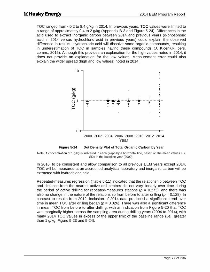
Submitted To 2014 EEM Program Report
Page 77 of 236
TOC ranged from <0.2 to 8.4 g/kg in 2014. In previous years, TOC values were limited to a range of approximately 0.4 to 2 g/kg (Appendix B-3 and Figure 5-24). Differences in the acid used to extract inorganic carbon between 2014 and previous years (o-phosphoric acid in 2014 versus hydrochloric acid in previous years) could explain the observed difference in results. Hydrochloric acid will dissolve some organic compounds, resulting in underestimation of TOC in samples having these compounds (J. Kiceniuk, pers. comm., 2015). Although this provides an explanation for the high values noted in 2014, it does not provide an explanation for the low values. Measurement error could also explain the wider spread (high and low values) noted in 2014.
2000 2002 2004 2006 2008 2010 2012 2014
Year
0.1
1
10T
OC
(g/k
g)
Figure 5-24 Dot Density Plot of Total Organic Carbon by Year
Note: A concentration of 1 g/kg is indicated in each graph by a horizontal line, based on the mean values + 2 SDs in the baseline year (2000).
In 2016, to be consistent and allow comparison to all previous EEM years except 2014, TOC will be measured at an accredited analytical laboratory and inorganic carbon will be extracted with hydrochloric acid.
Repeated-measures regression (Table 5-11) indicated that the relationship between TOC and distance from the nearest active drill centres did not vary linearly over time during the period of active drilling for repeated-measures stations (p = 0.273), and there was also no change in the nature of the relationship from before to after drilling (p = 0.128). In contrast to results from 2012, inclusion of 2014 data produced a significant trend over time in mean TOC after drilling began (p = 0.026). There was also a significant difference in mean TOC from before to after drilling, with an indication from Figure 5-20 that TOC was marginally higher across the sampling area during drilling years (2004 to 2014), with many 2014 TOC values in excess of the upper limit of the baseline range (i.e., greater than 1 g/kg; Figure 5-23 and 5-24).
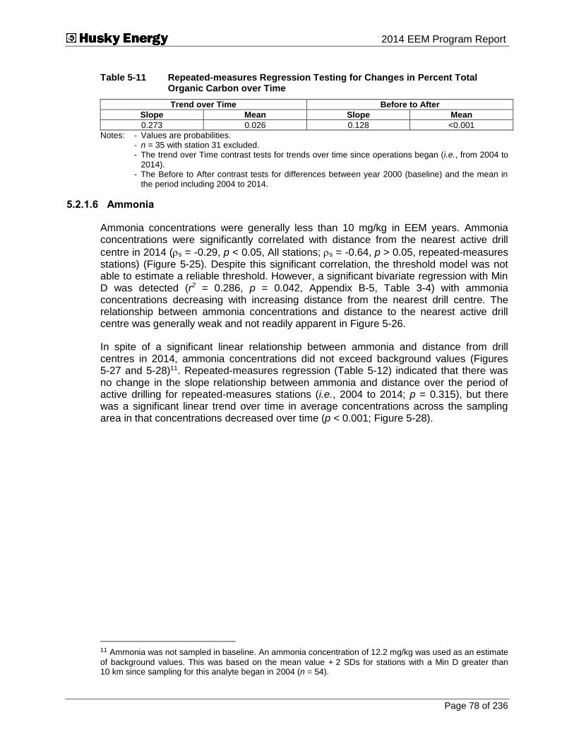
Submitted To 2014 EEM Program Report
Page 78 of 236
Table 5-11 Repeated-measures Regression Testing for Changes in Percent Total Organic Carbon over Time
Trend over Time Before to After
Slope Mean Slope Mean
0.273 0.026 0.128 <0.001
Notes: - Values are probabilities. - n = 35 with station 31 excluded. - The trend over Time contrast tests for trends over time since operations began (i.e., from 2004 to
2014). - The Before to After contrast tests for differences between year 2000 (baseline) and the mean in
the period including 2004 to 2014.
5.2.1.6 Ammonia
Ammonia concentrations were generally less than 10 mg/kg in EEM years. Ammonia concentrations were significantly correlated with distance from the nearest active drill
centre in 2014 (s = -0.29, p < 0.05, All stations; s = -0.64, p > 0.05, repeated-measures stations) (Figure 5-25). Despite this significant correlation, the threshold model was not able to estimate a reliable threshold. However, a significant bivariate regression with Min D was detected (r2 = 0.286, p = 0.042, Appendix B-5, Table 3-4) with ammonia concentrations decreasing with increasing distance from the nearest drill centre. The relationship between ammonia concentrations and distance to the nearest active drill centre was generally weak and not readily apparent in Figure 5-26.
In spite of a significant linear relationship between ammonia and distance from drill centres in 2014, ammonia concentrations did not exceed background values (Figures 5-27 and 5-28)11. Repeated-measures regression (Table 5-12) indicated that there was no change in the slope relationship between ammonia and distance over the period of active drilling for repeated-measures stations (i.e., 2004 to 2014; p = 0.315), but there was a significant linear trend over time in average concentrations across the sampling area in that concentrations decreased over time (p < 0.001; Figure 5-28).
11 Ammonia was not sampled in baseline. An ammonia concentration of 12.2 mg/kg was used as an estimate
of background values. This was based on the mean value + 2 SDs for stations with a Min D greater than 10 km since sampling for this analyte began in 2004 (n = 54).

Submitted To 2014 EEM Program Report
Page 79 of 236
RM Stations
All StationsAmmonia
2000 2002 2004 2006 2008 2010 2012 2014
Year
-1.0
-0.5
0.0
0.5
1.0
Sp
earm
an
Ran
k
Figure 5-25 Spearman Rank Correlations with Distance from the Nearest Active Drill Centre for Ammonia
Notes: Station 31 was excluded. n = 52 for All Stations n = 35 for Repeated-Measures (RM) Stations. Dotted lines indicate rank correlations of |0.3|, which were generally significant at p < 0.01, depending on sample
size in the given year; however, significance from specific statistical tests reported in text. Ammonia was not measured in the 2000 baseline survey.

Submitted To 2014 EEM Program Report
Page 80 of 236
0.1 1.0 10.0 100.0
Min D (km)
0
10
20
30
40
50
60
70
Am
monia
(m
g/k
g)
2004
0.1 1.0 10.0 100.0
Min D (km)
0
10
20
30
40
50
60
70
Am
monia
(m
g/k
g)
2005
0.1 1.0 10.0 100.0
Min D (km)
0
10
20
30
40
50
60
70
Am
monia
(m
g/k
g)
2006
0.1 1.0 10.0 100.0
Min D (km)
0
10
20
30
40
50
60
70
Am
monia
(m
g/k
g)
2008
0.1 1.0 10.0 100.0
Min D (km)
0
10
20
30
40
50
60
70
Am
monia
(m
g/k
g)
2010
0.1 1.0 10.0 100.0
Min D (km)
0
10
20
30
40
50
60
70
Am
monia
(m
g/k
g)
2012
0.1 1.0 10.0 100.0
Min D (km)
0
10
20
30
40
50
60
70
Am
monia
(m
g/k
g)
2014
Figure 5-26 Variations in Ammonia Concentrations with Distance from the Nearest
Active Drill Centre (all Years)
Notes: Min D = distance (km) to the nearest active drill centre. Ammonia was not measured the 2000 baseline survey. An ammonia concentration of 12.2 mg/kg was used as an estimate of background values. This was based on the mean value + 2 SDs for stations with a Min D greater than 10 km since sampling for
this analyte began in 2004 (n = 54).

Submitted To 2014 EEM Program Report
Page 81 of 236
Figure 5-27 Location of Stations with Ammonia Concentrations (2014) Within and Above the Background Range

Submitted To 2014 EEM Program Report
Page 82 of 236
2000 2004 2005 2006 2008 2010 2012 2014
Year
0.1
1.0
10.0
Am
mo
nia
(m
g/k
g)
Figure 5-28 Dot Density Plot of Ammonia Concentrations by Year
Note: A concentration of 12.2 mg/kg is indicated in each graph by a horizontal line, based on the mean values + 2 SDs for stations with a Min D greater than 10 km since sampling for this analyte began in 2004
(n = 54).
Table 5-12 Repeated-measures Regression Testing for Changes in Ammonia Concentrations over Time
Trend over Time Before to After
Slope Mean Slope Mean
0.315 <0.001 NA NA
Notes: - Values are probabilities. - n = 35 with station 31 excluded. - The trend over Time contrast tests for trends over time since operations began (i.e., from 2004 to
2014). - The Before to After contrast tests for differences between year 2000 (baseline) and the mean in
the period including 2004 to 2012. The Before to After contrast cannot be performed for ammonia as this variable was not measured during baseline.
5.2.1.7 Sulphide
Sulphide concentrations were generally less than 10 mg/kg in EEM years. Sulphide
concentrations were significantly correlated (s = -0.724, p < 0.001, All stations; s = -0.589, p < 0.001, repeated-measures stations) with distance from the nearest active drill centre in 2014 (Figure 5-29).

Submitted To 2014 EEM Program Report
Page 83 of 236
RM Stations
All StationsSulphide
2000 2002 2004 2006 2008 2010 2012 2014
Year
-1.0
-0.5
0.0
0.5
1.0
Spearm
an R
ank
2000 2002 2004 2006 2008 2010 2012 2014
-1.0
-0.5
0.0
0.5
1.0
Figure 5-29 Spearman Rank Correlations with Distance from the Nearest Active Drill
Centre for Sulphide
Notes: Station 31 was excluded. n = 52 for All Stations n = 35 for Repeated-Measures (RM) Stations. Dotted lines indicate rank correlations of |0.3|, which were generally significant at p < 0.01, depending on sample
size in the given year; however, significance from specific statistical tests reported in text. Sulphide was not measured in the 2000 baseline survey.
Despite a significant correlation with distance from the nearest active drill centre, the model was not able to estimate a reliable threshold in 2014. However, a significant bivariate regression with Min D was detected (r2 = 0.519; Appendix B-5, Table 3-4) with sulphide concentrations decreasing with increasing distance from the nearest drill centre. In 2006 and 2008, the threshold distances were estimated to be just greater than 1 km (Table 5-13). Figure 5-30 provides a graphical representation of threshold models.
Table 5-13 Results of Threshold Regressions on Distance from the Nearest Active Drill Centre for Sulphide
Year Threshold Distance (km)
2004 No threshold
2005 No threshold
2006 1.05 (0.74, 1.49)
2008 1.01 (0.64, 1.59)
2010 No threshold
2012 No threshold
2014 No threshold
Notes: - 95% confidence limits are provided in brackets. - n = 52 in 2014 with station 31 excluded.
Figure 5-31 corroborates the significant bivariate regression findings (Figure 5-30; Appendix B-5, Table 3-4) as well as the results of the Spearman rank correlations (Figure 5-29). Approximately 33% of stations exceeded the background range for sulphide in 2014, with the majority of these values found at stations nearest drill centres. Sulphide levels were elevated around the Central, North Amethyst, Southern and Northern Drill Centres. Sulphides were elevated at station 31, the site of an exploration well drilled in 2007. Sulphide levels were not elevated around the SWRX Drill Centre. Four stations more distant from drill centres have elevated sulphide levels.
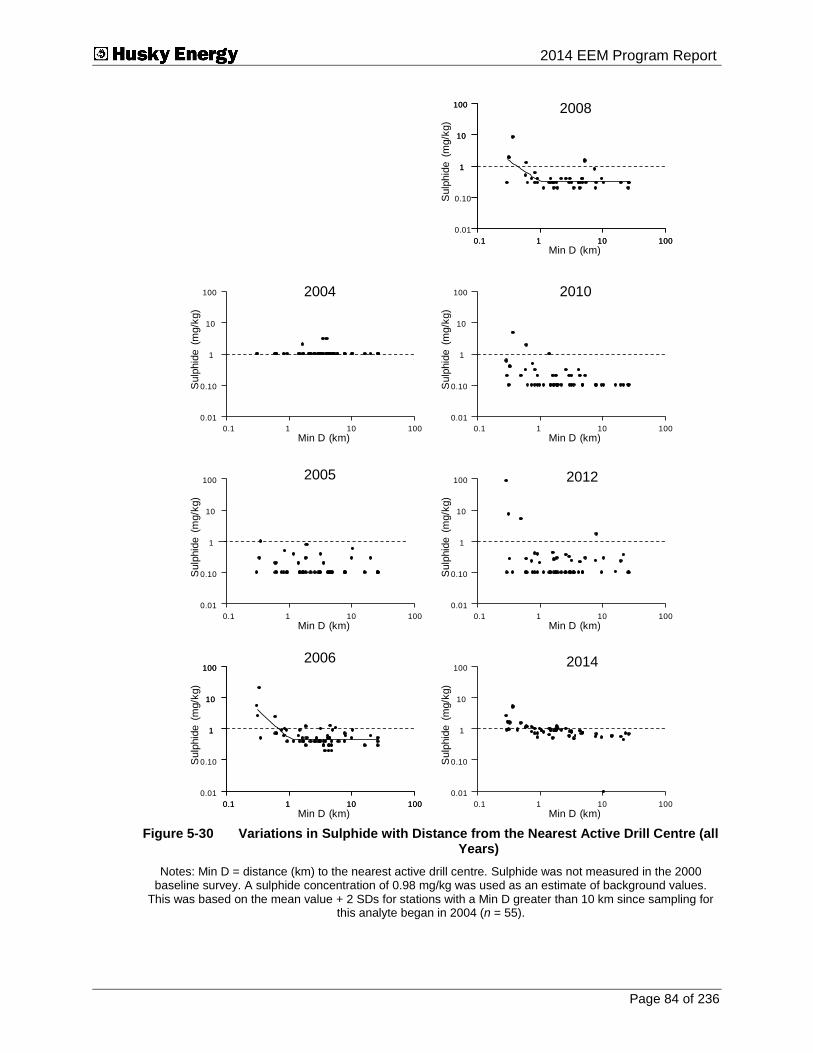
Submitted To 2014 EEM Program Report
Page 84 of 236
0.1 1 10 100
Min D (km)
0.01
0.10
1
10
100
Sulp
hid
e (
mg/k
g)
0.1 1 10 100
Min D (km)
0.01
0.10
1
10
100
Sulp
hid
e (
mg/k
g)
0.1 1 10 100
Min D (km)
1
10
100
Sulp
hid
e (
mg/k
g)
0.1 1 10 100
0.01
0.10
1
10
100
0.1 1 10 100
Min D (km)
0.01
0.10
1
10
100
Sulp
hid
e (
mg/k
g)
0.1 1 10 100
1
10
100
0.1 1 10 100
Min D (km)
0.01
0.10
1
10
100
Sulp
hid
e (
mg/k
g)
0.1 1 10 100
Min D (km)
0.01
0.10
1
10
100
Sulp
hid
e (
mg/k
g)
0.1 1 10 100
Min D (km)
0.01
0.10
1
10
100
Sulp
hid
e (
mg/k
g)
2004
2005
2006
2008
2010
2012
2014
Figure 5-30 Variations in Sulphide with Distance from the Nearest Active Drill Centre (all
Years)
Notes: Min D = distance (km) to the nearest active drill centre. Sulphide was not measured in the 2000 baseline survey. A sulphide concentration of 0.98 mg/kg was used as an estimate of background values.
This was based on the mean value + 2 SDs for stations with a Min D greater than 10 km since sampling for this analyte began in 2004 (n = 55).
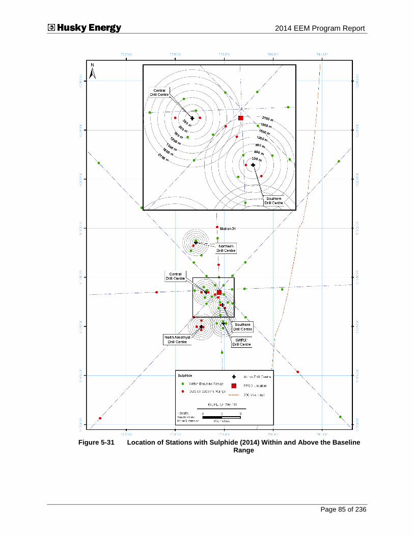
Submitted To 2014 EEM Program Report
Page 85 of 236
Figure 5-31 Location of Stations with Sulphide (2014) Within and Above the Baseline
Range

Submitted To 2014 EEM Program Report
Page 86 of 236
Repeated-measures regression (Table 5-14) indicated that there was a significant change in the slope relationship between sulphide and distance over the period of active drilling for repeated-measures stations (i.e., 2004 to 2014; p < 0.001), as well as a significant difference over time in average concentrations across the sampling area (i.e., decreasing concentrations over time, p < 0.001; Figure 5-32). Average sulphide concentrations in 2014 were the highest observed since 2004 (Figure 5-32).
Table 5-14 Repeated-measures Regression Testing for Changes in Sulphide Concentrations over Time
Trend over Time Before to After
Slope Mean Slope Mean
<0.001 0.001 NA NA
Notes: - Values are probabilities. - n = 35 with station 31 excluded. - The trend over Time contrast tests for trends over time since operations began (i.e., from 2004 to
2014). - The Before to After contrast tests for differences between year 2000 (baseline) and the mean in
the period including 2004 to 2012. The Before to After contrast cannot be performed for sulphide as this variable was not measured during baseline.
2000 2004 2005 2006 2008 2010 2012 2014
Year
0.01
0.10
1
10
100
Sulp
hid
e (
mg/k
g)
Figure 5-32 Dot Density Plot of Sulphide Concentrations by Year
Note: Sulphide was not measured in baseline. A concentration of 0.98 mg/kg is indicated in each graph by a horizontal line, based on the mean values + 2 SDs for stations with a Min D greater than 10 km since
sampling for this analyte began in 2004 (n = 55).

Submitted To 2014 EEM Program Report
Page 87 of 236
5.2.1.8 Sulphur
Sulphur and distance to the nearest active drill centre were significantly correlated (s =
-0.53, p < 0.001, All stations; s = -0.36, p < 0.05, repeated-measures stations; Figure 5-33). Despite this significant correlation, the threshold model was not able to estimate a reliable threshold. However, a significant bivariate regression with Min D was detected (r2 = 0.448, p = 0.001, Appendix B-5, Table 3-4) with sulphur concentrations decreasing with increasing distance from the nearest drill centre. The relationship between sulphur concentrations and distance to the nearest active drill centre is illustrated in Figure 5-34. Sulphur was elevated around the Central, North Amethyst and Southern Drill Centres (Figure 5-35).
RM Stations
All StationsSulphur
2000 2002 2004 2006 2008 2010 2012 2014
Year
-1.0
-0.5
0.0
0.5
1.0
Sp
earm
an
Ran
k
Figure 5-33 Spearman Rank Correlations with Distance from the Nearest Active Drill Centre for Sulphur
Notes: Station 31 was excluded. n = 52 for All Stations. n = 35 for Repeated-Measures (RM) Stations. Dotted lines indicate rank correlations of |0.3|, which were generally significant at p < 0.01, depending on sample
size in the given year; however, significance from specific statistical tests reported in text.

Submitted To 2014 EEM Program Report
Page 88 of 236
0.1 1.0 10.0 100.0
Min D (km)
0.0
0.1
0.2
0.3
0.4
0.5
Sulp
hur
(%)
2004
0.1 1.0 10.0 100.0
Min D (km)
0.0
0.1
0.2
0.3
0.4
0.5
Sulp
hur
(%)
2005
0.1 1.0 10.0 100.0
Min D (km)
0.0
0.1
0.2
0.3
0.4
0.5
Sulp
hur
(%)
2006
0.1 1.0 10.0 100.0
Min D (km)
0.0
0.1
0.2
0.3
0.4
0.5
Sulp
hur
(%)
2008
0.1 1.0 10.0 100.0
Min D (km)
0.0
0.1
0.2
0.3
0.4
0.5
Sulp
hur
(%)
2010
0.1 1.0 10.0 100.0
Min D (km)
0.0
0.1
0.2
0.3
0.4
0.5
Sulp
hur
(%)
2012
0.1 1.0 10.0 100.0
Min D (km)
0.0
0.1
0.2
0.3
0.4
0.5
Sulp
hur
(%)
2014
Figure 5-34 Variations in Sulphur Concentrations with Distance from the Nearest Active
Drill Centre (all Years)
Note: Min D = distance (km) to the nearest active drill centre. Sulphur was not measured in the 2000 baseline survey. A concentration of 0.05 % is indicated in each graph by a horizontal line, based on the
mean values + 2 SDs for stations with a Min D greater than 10 km since sampling for this analyte began in 2004 (n = 55).

Submitted To 2014 EEM Program Report
Page 89 of 236
Figure 5-35 Location of Stations with Sulphur (2014) Within and Above the Background Range
Repeated-measures regression (Table 5-15) indicated that there was no change in the slope of the relationship between sulphur and distance from active drill centres over the drilling period for repeated-measures stations (p = 0.365). There was a significant linear time trend in average sulphur concentrations (increasing) in the overall sampling area (p < 0.001). The dot density graph of percent sulphur (Figure 5-36) illustrated that mean
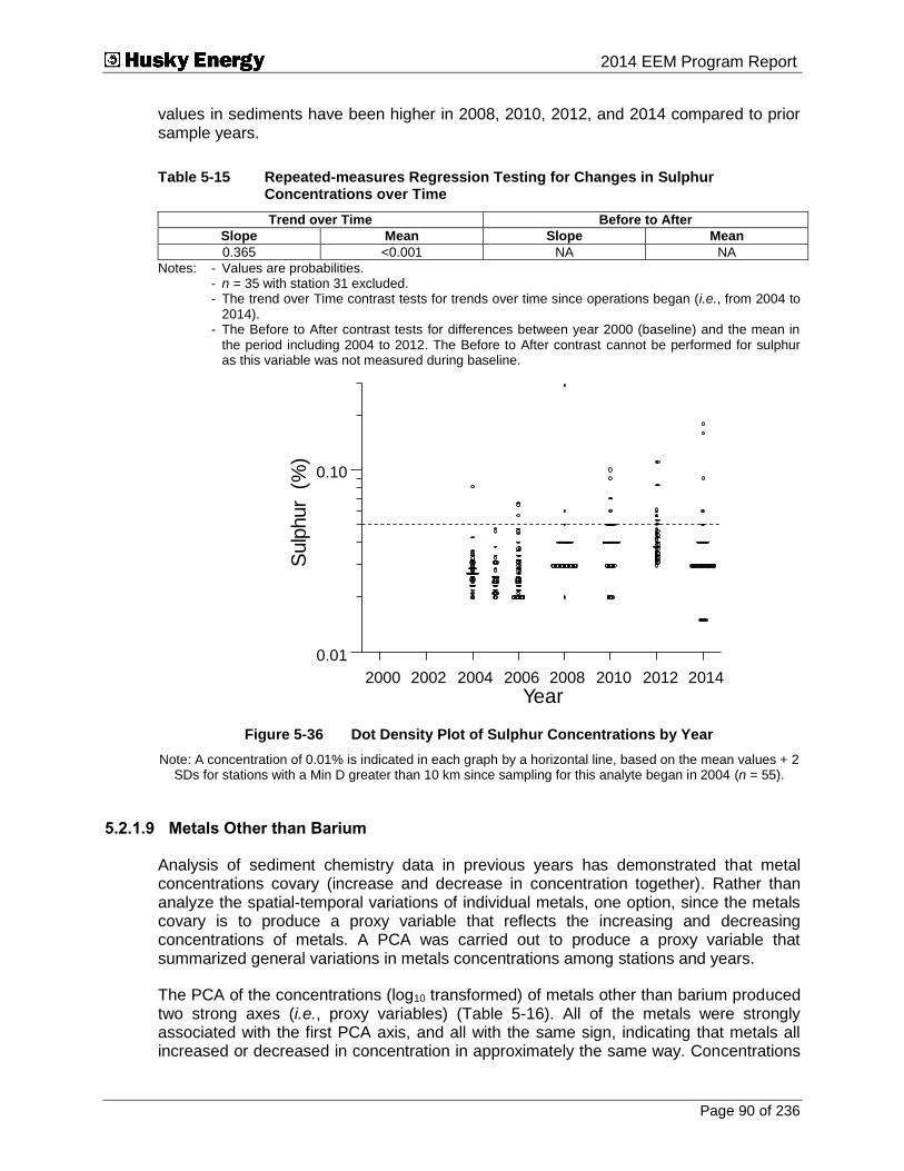
Submitted To 2014 EEM Program Report
Page 90 of 236
values in sediments have been higher in 2008, 2010, 2012, and 2014 compared to prior sample years.
Table 5-15 Repeated-measures Regression Testing for Changes in Sulphur Concentrations over Time
Trend over Time Before to After
Slope Mean Slope Mean
0.365 <0.001 NA NA
Notes: - Values are probabilities. - n = 35 with station 31 excluded. - The trend over Time contrast tests for trends over time since operations began (i.e., from 2004 to
2014). - The Before to After contrast tests for differences between year 2000 (baseline) and the mean in
the period including 2004 to 2012. The Before to After contrast cannot be performed for sulphur as this variable was not measured during baseline.
2000 2002 2004 2006 2008 2010 2012 2014
Year
0.01
0.10
Sulp
hur
(%)
Figure 5-36 Dot Density Plot of Sulphur Concentrations by Year
Note: A concentration of 0.01% is indicated in each graph by a horizontal line, based on the mean values + 2 SDs for stations with a Min D greater than 10 km since sampling for this analyte began in 2004 (n = 55).
5.2.1.9 Metals Other than Barium
Analysis of sediment chemistry data in previous years has demonstrated that metal concentrations covary (increase and decrease in concentration together). Rather than analyze the spatial-temporal variations of individual metals, one option, since the metals covary is to produce a proxy variable that reflects the increasing and decreasing concentrations of metals. A PCA was carried out to produce a proxy variable that summarized general variations in metals concentrations among stations and years.
The PCA of the concentrations (log10 transformed) of metals other than barium produced two strong axes (i.e., proxy variables) (Table 5-16). All of the metals were strongly associated with the first PCA axis, and all with the same sign, indicating that metals all increased or decreased in concentration in approximately the same way. Concentrations

Submitted To 2014 EEM Program Report
Page 91 of 236
of strontium and lead were also strongly correlated with the second PCA axis indicating that those metals, independently of the others, covaried in relation to other factors. Scores on the first PCA axis were used as the proxy variable (Metals PC1) summarizing variations in metals concentrations in subsequent analyses. Lead and strontium, which correlated strongly with the second PCA axis, were analyzed separately.
Table 5-16 Principal Component Analysis Component Loadings (Correlations) of Metals Concentrations
Variable Principal Component
1 2
Aluminum 0.781 -0.144
Chromium 0.791 0.190
Iron 0.905 0.321
Lead 0.589 -0.726
Manganese 0.846 0.403
Strontium 0.739 -0.621
Uranium 0.685 0.003
Vanadium 0.822 0.262
Percent Variance Explained 60.1 16.3
Notes: - |r| 0.6 in bold. n = 52, with station 31 excluded.
Metals PC1
Metals PC1 scores were not correlated with distance from the nearest active drill centre
in 2014 (s = 0.02, p > 0.05, All stations; (s = 0.185, p > 0.05, repeated-measures stations; Figure 5-37).
RM Stations
All StationsMetals PC1
2000 2002 2004 2006 2008 2010 2012 2014
Year
-1.0
-0.5
0.0
0.5
1.0
Sp
earm
an
Ran
k
Figure 5-37 Spearman Rank Correlations with Distance from the Nearest Active Drill Centre for Metals PC1
Notes: Station 31 was excluded. n = 52 for All Stations n = 35 for Repeated-Measures (RM) Stations. Dotted lines indicate rank correlations of |0.3|, which were generally significant at p < 0.01, depending on sample
size in the given year; however, significance from specific statistical tests reported in text.
Figure 5-38 provides a graphical representation of Metals PC1 scores with distance from active drill centres.

Submitted To 2014 EEM Program Report
Page 92 of 236
0.1 1 10 100
Min D (km)
-3
-2
-1
0
1
2
3
4
Meta
ls P
C 1
0.1 1 10 100
Min D (km)
-3
-2
-1
0
1
2
3
4
Meta
ls P
C 1
2004
0.1 1 10 100
Min D (km)
-3
-2
-1
0
1
2
3
4
Meta
ls P
C 1
2005
0.1 1 10 100
Min D (km)
-3
-2
-1
0
1
2
3
4
Meta
ls P
C 1
2006
0.1 1 10 100
Min D (km)
-3
-2
-1
0
1
2
3
4
Meta
ls P
C 1
2008
0.1 1 10 100
Min D (km)
-3
-2
-1
0
1
2
3
4
Meta
ls P
C 1
2010
0.1 1 10 100
Min D (km)
-3
-2
-1
0
1
2
3
4
Meta
ls P
C 1
2012
0.1 1 10 100
Min D (km)
-3
-2
-1
0
1
2
3
4
Meta
ls P
C 1
2014
2000
Figure 5-38 Variations in Metals PC1 Scores with Distance from the Nearest Active Drill Centre (all Years)
Notes: Min D = distance (km) to the nearest active drill centre, except in 2000 (baseline), where Min D is distance to the nearest future drill centre. Background PC1 scores (-2 and 2) are indicated by a horizontal
line, based on the mean values ± 2 SDs using data from 2000.

Submitted To 2014 EEM Program Report
Page 93 of 236
Repeated-measures regression (Table 5-17) indicated that there was no change in the slope of the relationship between Metals PC1 scores and distance to the nearest active drill centre over the active drilling period for repeated-measures stations (p = 0.855), and no change in the slope from before to after drilling began (p = 0.593). There were also no significant variations in the average PC1 axis scores in the overall sampling area (p = 0.359), and no difference from before drilling to after drilling began (p = 0.488).
Table 5-17 Repeated-measures Regression Testing for Changes in Metals PC1 scores over Time
Trend over Time Before to After
Slope Mean Slope Mean
0.855 0.359 0.593 0.488
Notes: - Values are probabilities.
- n = 35 with station 31 excluded.
- The trend over Time contrast tests for trends over time since operations began (i.e., from 2004 to
2014).
- The Before to After contrast tests for differences between year 2000 (baseline) and the mean in
the period including 2004 to 2014.
The dot density graph of scores (Figure 5-39) further illustrated that Metals PC1 scores were consistent across years, with scores in 2014 mostly within the baseline range of variation for scores in 2000.
2000 2002 2004 2006 2008 2010 2012 2014
Year
-4
-3
-2
-1
0
1
2
3
4
Me
tals
PC
1
Figure 5-39 Dot Density Plot of Metals PC1 Scores by Year
Note: Background PC1 scores are indicated by a horizontal line, based on the mean values ± 2 SDs using data from the baseline year (2000).

Submitted To 2014 EEM Program Report
Page 94 of 236
Lead
Lead concentrations in sediments were negatively correlated with distance to the nearest
active drill centre in 2014 (s = -0.32, p < 0.05, All stations; s = -0.41, p < 0.05, repeated-measures stations), similar to what was observed in 2006, 2008, and 2012 (Figure 5-40). A threshold distance explained significant variation in the distance relationship in each of the surveys from 2006 to 2014 (Appendix B-5), with the threshold distance typically near 1 km. The threshold distance decreased consistently from 2006 (1.5 km) to 2014 (0.6 km) (Table 5-18). The relationship between lead concentrations and Min D is illustrated in Figure 5-41. In 2014, lead was enriched around the Central and Southern Drill Centres (Figure 5-42).
RM Stations
All StationsLead
2000 2002 2004 2006 2008 2010 2012 2014
Year
-1.0
-0.5
0.0
0.5
1.0
Sp
earm
an
Ran
k
Figure 5-40 Spearman Rank Correlations with Distance from the Nearest Active Drill Centre for Lead
Notes: Station 31 was excluded. n = 52 for All Stations. n = 35 for Repeated-Measures (RM) Stations. Dotted lines indicate rank correlations of |0.3|, which were generally significant at p < 0.01,
depending on sample size in the given year; however, significance from specific statistical tests reported in text.
Table 5-18 Results of Threshold Regressions on Distance from the Nearest Active Drill Centre for Lead
Year Threshold Distance (km)
2004 No threshold
2005 No threshold
2006 1.5 (1.0, 2.3)
2008 1.1 (0.7, 1.7)
2010 0.9 (0.6, 1.4)
2012 0.6 (0.5, 0.8)
2014 0.6 (0.4, 1.0)
Notes: - 95% confidence limits are provided in brackets. - n = 52 in 2014 with station 31 excluded.

Submitted To 2014 EEM Program Report
Page 95 of 236
0.1 1 10 100
Min D (km)
1
10
Lead (
mg/k
g)
0.1 1 10 100
Min D (km)
1
10
Lead (
mg/k
g)
0.1 1 10 100
Min D (km)
1
10
Lead (
mg/k
g)
0.1 1 10 100
Min D (km)
1
10
Lead (
mg/k
g)
0.1 1 10 100
0.1 1 10 100
Min D (km)
1
10
Lead (
mg/k
g)
0.1 1 10 100
0.1 1 10 100
Min D (km)
1
10
Lead (
mg/k
g)
0.1 1 10 100
0.1 1 10 100
Min D (km)
1
10
Lead (
mg/k
g)
0.1 1 10 100
0.1 1 10 100
Min D (km)
1
10
Lead (
mg/k
g)
0.1 1 10 100
2000 2008
2004 2010
2005 2012
2006 2014
Figure 5-41 Variations in Lead with Distance from the Nearest Active Drill Centre (all Years)
Notes: Min D = distance (km) to the nearest active drill centre, except in 2000 (baseline), where Min D is distance to the nearest future drill centre. Background concentrations of 2.1 and 3.7 mg/kg are indicated by
horizontal lines, based on the mean values ± 2 SDs from 2000 (baseline), respectively.

Submitted To 2014 EEM Program Report
Page 96 of 236
Figure 5-42 Location of Stations with Lead (2014) Within and Above the Baseline Range
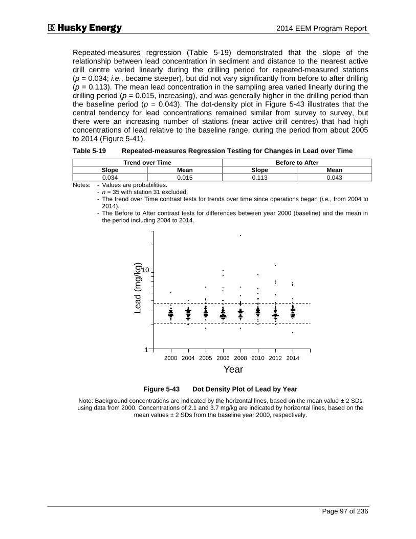
Submitted To 2014 EEM Program Report
Page 97 of 236
Repeated-measures regression (Table 5-19) demonstrated that the slope of the relationship between lead concentration in sediment and distance to the nearest active drill centre varied linearly during the drilling period for repeated-measured stations (p = 0.034; i.e., became steeper), but did not vary significantly from before to after drilling (p = 0.113). The mean lead concentration in the sampling area varied linearly during the drilling period (p = 0.015, increasing), and was generally higher in the drilling period than the baseline period (p = 0.043). The dot-density plot in Figure 5-43 illustrates that the central tendency for lead concentrations remained similar from survey to survey, but there were an increasing number of stations (near active drill centres) that had high concentrations of lead relative to the baseline range, during the period from about 2005 to 2014 (Figure 5-41).
Table 5-19 Repeated-measures Regression Testing for Changes in Lead over Time
Trend over Time Before to After
Slope Mean Slope Mean
0.034 0.015 0.113 0.043
Notes: - Values are probabilities. - n = 35 with station 31 excluded. - The trend over Time contrast tests for trends over time since operations began (i.e., from 2004 to
2014). - The Before to After contrast tests for differences between year 2000 (baseline) and the mean in
the period including 2004 to 2014.
2000 2004 2005 2006 2008 2010 2012 2014
Year
1
10
Lea
d (
mg
/kg
)
Figure 5-43 Dot Density Plot of Lead by Year
Note: Background concentrations are indicated by the horizontal lines, based on the mean value ± 2 SDs using data from 2000. Concentrations of 2.1 and 3.7 mg/kg are indicated by horizontal lines, based on the
mean values ± 2 SDs from the baseline year 2000, respectively.

Submitted To 2014 EEM Program Report
Page 98 of 236
Strontium
Strontium concentrations in sediments were not significantly correlated with distance to
the nearest active drill centre in 2014 (s = -0.23, p > 0.05, All stations; s = -0.14, p > 0.05, repeated-measures stations). This contrasts with trends observed between 2004 and 2012 (for All stations; Figure 5-44). The relationship between strontium concentrations and distance to the nearest active drill centre is illustrated in Table 5-20 and Figure 5-45. Threshold distances, when detected, were variable (Figure 5-45) yet still maintain overlapping 95% confidence intervals (Table 5-20).
RM Stations
All StationsStrontium
2000 2002 2004 2006 2008 2010 2012 2014
Year
-1.0
-0.5
0.0
0.5
1.0S
pearm
an
Ran
k
Figure 5-44 Spearman Rank Correlations with Distance from the Nearest Active Drill Centre for Strontium
Notes: Station 31 was excluded. n = 52 for All Stations n = 35 for Repeated-Measures (RM) Stations. Dotted lines indicate rank correlations of |0.3|, which were generally significant at p < 0.01, depending on sample
size in the given year; however, significance from specific statistical tests reported in text.
Table 5-20 Results of Threshold Regressions on Distance from the Nearest Active Drill Centre for Strontium
Year Threshold Distance (km)
2004 No threshold
2005 No threshold
2006 1.2 (0.7, 1.8)
2008 1.6 (0.7, 3.6)
2010 No threshold
2012 0.6 (0.5, 0.9)
2014 No threshold
Notes: - 95% confidence limits are provided in brackets. - n = 52 in 2012 with station 31 excluded.
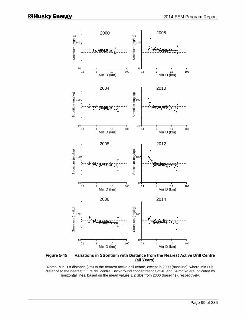
Submitted To 2014 EEM Program Report
Page 99 of 236
0.1 1 10 100
Min D (km)
10
100
Str
ontium
(m
g/k
g)
0.1 1 10 100
Min D (km)
10
100
Str
ontium
(m
g/k
g)
0.1 1 10 100
Min D (km)
10
100
Str
ontium
(m
g/k
g)
0.1 1 10 100
Min D (km)
10
100
Str
ontium
(m
g/k
g)
0.1 1 10 100
1 10 100
Min D (km)
10
100
Str
ontium
(m
g/k
g)
0.1 1 10 100
0.1 1 10 100
Min D (km)
10
100
Str
ontium
(m
g/k
g)
0.1 1 10 100
Min D (km)
100
Str
ontium
(m
g/k
g)
0.1 1 10 100
10
0.1 1 10 100
Min D (km)
10
100
Str
ontium
(m
g/k
g)
2000 2008
2004 2010
2005 2012
2006 2014
Figure 5-45 Variations in Strontium with Distance from the Nearest Active Drill Centre (all Years)
Notes: Min D = distance (km) to the nearest active drill centre, except in 2000 (baseline), where Min D is distance to the nearest future drill centre. Background concentrations of 40 and 54 mg/kg are indicated by
horizontal lines, based on the mean values ± 2 SDs from 2000 (baseline), respectively.
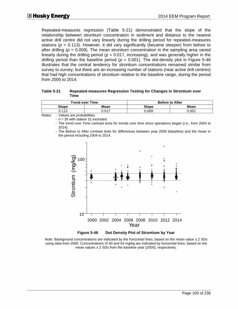
Submitted To 2014 EEM Program Report
Page 100 of 236
Repeated-measures regression (Table 5-21) demonstrated that the slope of the relationship between strontium concentration in sediment and distance to the nearest active drill centre did not vary linearly during the drilling period for repeated-measures stations (p = 0.113). However, it did vary significantly (became steeper) from before to after drilling (p = 0.009). The mean strontium concentration in the sampling area varied linearly during the drilling period (p = 0.017, increasing), and was generally higher in the drilling period than the baseline period (p = 0.001). The dot-density plot in Figure 5-46 illustrates that the central tendency for strontium concentrations remained similar from survey to survey, but there are an increasing number of stations (near active drill centres) that had high concentrations of strontium relative to the baseline range, during the period from 2005 to 2014.
Table 5-21 Repeated-measures Regression Testing for Changes in Strontium over Time
Trend over Time Before to After
Slope Mean Slope Mean
0.113 0.017 0.009 0.001
Notes: - Values are probabilities. - n = 35 with station 31 excluded. - The trend over Time contrast tests for trends over time since operations began (i.e., from 2004 to
2014). - The Before to After contrast tests for differences between year 2000 (baseline) and the mean in
the period including 2004 to 2014.
2000 2002 2004 2006 2008 2010 2012 2014
Year
10
100
Str
ontium
(m
g/k
g)
Figure 5-46 Dot Density Plot of Strontium by Year
Note: Background concentrations are indicated by the horizontal lines, based on the mean value ± 2 SDs using data from 2000. Concentrations of 40 and 54 mg/kg are indicated by horizontal lines, based on the
mean values ± 2 SDs from the baseline year (2000), respectively.

Submitted To 2014 EEM Program Report
Page 101 of 236
5.2.1.10 Redox Potential
Redox potential varied between 194 and 303 mV in 2014, and was significantly and
positively correlated with distance from the nearest active drill centre (s = 0.43, p < 0.01,
All stations; s = 0.35, p < 0.05, repeated-measures stations) (Figure 5-47). Despite this significant correlation, the threshold model was not able to estimate a reliable threshold. However, a significant bivariate regression with Min D was detected (r2 = 0.485, p < 0.001, Appendix B-5, Table 3-4) with redox potential increasing with increasing distance from the nearest drill centre. The relationship between redox potential and distance to the nearest active drill centre is illustrated in Figure 5-48.
RM Stations
All StationsRedox
2000 2002 2004 2006 2008 2010 2012 2014
Year
-1.0
-0.5
0.0
0.5
1.0
Spe
arm
an R
an
k
2000 2002 2004 2006 2008 2010 2012 2014
-1.0
-0.5
0.0
0.5
1.0
Figure 5-47 Spearman Rank Correlations with Distance from the Nearest Active Drill Centre for Redox Potential
Notes: Station 31 was excluded. n = 52 for All Stations. n = 35 for Repeated-Measures Stations. Dotted lines indicate rank correlations of |0.3|, which were generally significant at p < 0.01, depending on sample size in
the given year; however, significance from specific statistical tests reported in text.
The scatterplots of redox potential with distance from active drill centres are provided in Figure 5-48. There was a modest tendency for redox potential to be greater at stations further from the nearest active drill centre, and for that tendency to increase over time. However, only a single station (S5, redox potential = 194 mV) immediately adjacent to a drill centre was below the baseline range (207-294 mV; Figure 5-49).
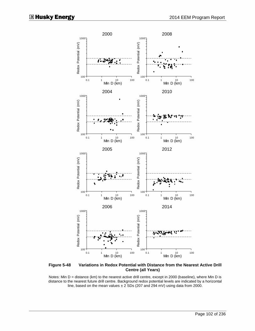
Submitted To 2014 EEM Program Report
Page 102 of 236
0.1 1 10 100
Min D (km)
100
1000
Redox P
ote
ntial
(mV
)
2000
0.1 1 10 100
Min D (km)
100
1000
Redox P
ote
ntial
(mV
)
2004
0.1 1 10 100
Min D (km)
100
1000
Redox P
ote
ntial
(mV
)
2005
0.1 1 10 100
Min D (km)
100
1000
Redox P
ote
ntial
(mV
)
2006
0.1 1 10 100
Min D (km)
100
1000
Redox P
ote
ntial
(mV
)
2008
0.1 1 10 100
Min D (km)
100
1000
Redox P
ote
ntial
(mV
)
2010
0.1 1 10 100
Min D (km)
100
1000
Redox P
ote
ntial
(mV
)
2012
0.1 1 10 100
Min D (km)
100
1000
Redox P
ote
ntial
(mV
)
2014
Figure 5-48 Variations in Redox Potential with Distance from the Nearest Active Drill Centre (all Years)
Notes: Min D = distance (km) to the nearest active drill centre, except in 2000 (baseline), where Min D is distance to the nearest future drill centre. Background redox potential levels are indicated by a horizontal
line, based on the mean values ± 2 SDs (207 and 294 mV) using data from 2000.

Submitted To 2014 EEM Program Report
Page 103 of 236
Figure 5-49 Location of Stations with Redox Potential (2014) Within and Above the Baseline Range

Submitted To 2014 EEM Program Report
Page 104 of 236
Repeated-measures regression (Table 5-22) indicated that there was no significant change in the slope of the relationship between redox potential and distance to the nearest active drill centre during drilling years for repeated-measures stations (p = 0.145). However, there was a significant linear trend over time in mean redox potential across the sampling area (p = 0.015), and from before to after drilling (p = 0.001).
Table 5-22 Repeated-measures Regression Testing for Changes in Redox Potential over Time
Trend over Time Before to After
Slope Mean Slope Mean
0.145 0.015 0.367 0.001
Notes: - Values are probabilities. - n = 35 with station 31 excluded. - The trend over Time contrast tests for trends over time since operations began (i.e., from 2004 to
2014). - The Before to After contrast tests for differences between year 2000 (baseline) and the mean in
the period including 2004 to 2014.
The dot density graph (Figure 5-50) illustrated that redox values were generally higher in 2014 than in 2012, and comparable to the baseline period (year 2000). While redox potential has varied with time, all sediments since baseline have been oxic.
2000 2002 2004 2006 2008 2010 2012 2014
Year
100
1000
Re
do
x (
mV
)
Figure 5-50 Dot Density Plot of Redox Potential by Year
Note: Background concentrations are indicated by the horizontal lines, based on the mean value ± 2 SDs using data from 2000. Thresholds of 207 mV and 294 mV are indicated by horizontal lines, based on the
mean values ± 2 SDs from the baseline year (2000), respectively.

Submitted To 2014 EEM Program Report
Page 105 of 236
5.2.2 Toxicity
In 2014, three samples were toxic to bacterial luminescence. A single toxic sample was noted in 2010. No toxic response was noted in other years. Toxicity in 2014 occurred at stations 19, N1 and N2. Station 19 is a reference station and is located 22 km from the nearest drill centre. Stations N1 and N2 are located 2.2 and 1.5 km from the Northern Drill Centre, respectively. Full test results bacterial luminescence toxicity for 2014 are provided in Appendix B-6. No analysis is provided as too few samples were toxic to bacterial luminescence.
For amphipod toxicity testing of sediment, amphipod survival was greater than 80% for all but two samples. For this EEM program, samples were considered toxic if they were more than 20% lower in terms of survival than the site reference, WRRS. Survival in WRRS was 97% and only two samples had more than 20% reduced survival and were significantly different from WRRS: station C1, located 1.1 km from the Central Drill Centre, had 64% survival, and station 16, located 5.59 km from the North Amethyst Drill Centre had 76% survival. In 2000, 2004 and 2010, no sediments were considered toxic; in 2005, sediment from one station was considered toxic; in 2006, sediment from three stations were considered toxic; in 2008, sediment from eight stations were considered toxic; and in 2012, sediment from one station was considered toxic according to the amphipod survival test. Full results for amphipod toxicity for 2014 are provided in Appendix B-7. A review of the sediment chemistry and particle size results does not reveal any apparent cause for the toxicity.
Percent survival in 2014 was not significantly correlated with any assessed variables (p > 0.05; Table 5-23).
Table 5-23 Spearman Rank Correlations (s) Between Amphipod Survival versus Distance from the Nearest Active Drill Centre and Sediment Physical and Chemical Characteristics (2014)
Variable Spearman Rank Correlation (s) with Amphipod Survival
Distance from nearest active drill centre -0.120
>C10–C21 hydrocarbons 0.117
Barium 0.079
% Fines 0.204
% Gravel -0.001
TOC -0.019
Metals PC1 -0.121
Lead -0.008
Strontium 0.030
Ammonia 0.079
Sulphur 0.153
Notes: - *p 0.05; **p 0.01; ***p 0.001 (in bold).
- n = 53 stations.
The 2014 data, and toxicity data from prior years, suggest little change over time. Variation in amphipod survival was somewhat higher in 2005, 2006 and 2008, and was similar in 2014 to what was observed in 2000 (baseline), 2004, 2010, and 2012 (Figure 5-51).

Submitted To 2014 EEM Program Report
Page 106 of 236
2000 2002 2004 2006 2008 2010 2012 2014
Year
0
20
40
60
80
100
Am
phip
od S
urv
iva
l (%
)
Figure 5-51 Dot Density Plot of Laboratory Amphipod Survival by Year
Note: The horizontal line denotes 70% survival. Values above 70% indicate a non-toxic response.
5.2.3 Benthic Community Structure
5.2.3.1 General Composition
Raw data for benthic community structure in 2014 are provided in Appendix B-4. A total of 219 taxa, from 87 families, were identified from 106 samples collected from 53 stations in 2014. As in prior years, Polychaeta were numerically dominant, accounting for 67% of total numbers, while Bivalvia (16%), Amphipoda (2%) and Tellinidae (3%) were sub-dominant numerically, and Cnidaria, Gastropoda, Cirrepedia, Cumacea, Decapoda, Echinodermata, Hemichordata and Urochordata were found in trace numbers (1% or less).
Table 5-24 lists all families and their associated higher taxonomic classifications that represented 1% or more of the total number of organisms collected in all sample years. Polychaetes in the family Spionidae (primarily Prionospio steenstrupi and several Spio species) were the most abundant (dominant) family in 2014, as in prior years. Bivalves were dominated by the family Tellinidae (primarily Macoma calcarea) in 2014, again as in prior years.

Submitted To 2014 EEM Program Report
Page 107 of 236
Table 5-24 Relative Abundance of Dominant Benthic Invertebrates Major Groups
Major Taxon Class or Order Family Year
2000 2004 to 2012 2014
Porifera <1
Cnidaria <1 <1 <1
Annelida Polychaeta
Total 77 72 to 81 67
Maldanidae 1 2 2
Orbiniidae 5 4 to 6 5
Paraonidae 15 10 to 21 10
Phyllodocidae 3 3 to 6 2
Spionidae 37 35 to 48 33
Syllidae 1 1 to 2 1
Capitellidae 1 1 to 2 1
Cirratulidae 13 1 to 2 2
Mollusca Bivalvia
Total 17 12 to 18 16
Tellinidae 13 10 to 16 13
Gastropoda
<1 <1 to 1 1
Crustacea
Total 4 5 to 7 5
Amphipoda 3 2 to 3 2
Isopoda Total 1 2 to 4 <1
Tanaidacea 1 2 to 3 3
Cirrepedia <1 <1 <1
Cumacea <1 <1 <1
Decapoda <1 0 to <1 <1
Echinodermata 1 1 to 2 1
Hemichordata 0 to <1 <1
Urochordata 0 to <1
5.2.3.2 Correlations with Sediment Physical and Chemical Characteristics
In 2014, none of the indices of benthic community composition were significantly related to percent of substrate as gravel (% gravel), TOC, metals PC1, or laboratory amphipod survival (Table 5-25). However, there were a variety of significant correlations between indices of benthic community composition and other environmental descriptors. Total abundance, biomass and Paraoniade abundance were significantly correlated with distance to the nearest active drill centre. These and in-situ amphipod abundance were significantly correlated with sediment concentrations of >C10-C21 hydrocarbons. Biomass, richness and Paraonidae abundance were significantly correlated with sediment barium concentrations. Biomass, Paraonidae and amphipod abundance were significantly correlated with sediment sulphur concentrations. Biomass, richness and Paraonidae abundance were significantly correlated with sediment lead concentrations. Richness and Paraoniade abundance were significantly correlated with sediment strontium concentrations. Richness was correlated with sediment % fines content, and Paraonidae abundance was correlated with water depth. Most of those same correlations were statistically significant in 2012, as well as in 2010, and reflect consistent relationships over the last three EEM surveys. Benthic community variables were analyzed in greater detail in Sections 5.2.3.3 to 5.2.3.6.

Submitted To 2014 EEM Program Report
Page 108 of 236
Table 5-25 Spearman Rank Correlations (S) of Indices of Benthic Community Composition with Environmental Descriptors (2014)
Environmental Descriptor
Index of Invertebrate Community Composition
To
tal
Ab
un
da
nce
Bio
ma
ss
Ric
hn
ess
Pa
rao
nid
ae
Ab
un
da
nce
Sp
ion
idae
Ab
un
da
nce
Te
llin
ida
e
Ab
un
da
nce
Am
ph
ipo
da
Ab
un
da
nce
% Fines 0.148 -0.190 0.289** -0.473 0.197 0.166 0.259
% Gravel 0.054 0.004 0.177 -0.048 0.057 -0.090 0.136
TOC -0.001 -0.188 0.132 -0.094 -0.074 0.127 -0.006
>C10-C21 -0.297* -0.571* 0.112 -0.816* 0.079 -0.096 0.275*
Barium -0.082 -0.399*** 0.272* -0.603*** 0.100 -0.098 0.268
Metals PC1 0.224 0.076 0.252 0.045 0.047 0.140 -0.049
Lead 0.009 -0.288* 0.301* -0.369** 0.065 -0.124 0.212
Strontium 0.128 -0.225 0.282* -0.276* 0.053 0.037 0.143
Sulphur 0.071 -0.393** 0.117 -0.609*** 0.201 0.201 0.377**
Redox Potential 0.002 0.249 -0.115 0.318* -0.072 0.014 -0.097
Distance to nearest active drill centre
0.304* 0.573*** -0.149 0.765*** -0.047 0.051 -0.208
Laboratory Amphipod survival
0.118 0.130 -0.126 -0.061 0.046 0.162 0.012
Water Depth 0.121 0.259 0.103 0.271* 0.074 -0.084 -0.144
Notes: - *p < 0.05; **p < 0.01; ***p < 0.001 (in bold).
- n = 53. - Shaded cells also produced significant correlations in the 2012 data set.
5.2.3.3 Total Abundance
In 2014, total abundance of all benthic invertebrates varied between approximately 1,000 organisms per m² to over 6,200 per m² across the sampling area. The relationship between total abundance and distance from the nearest active drill centre was significant
in 2014 (s = 0.30, p < 0.05, All stations; s = 0.42, p = 0.01, repeated-measures stations), with comparable significance noted in 2005, 2006, 2008 and 2012 (Figure 5-52). While the data did not allow for precise estimation of a threshold (Appendix B-5), a significant bivariate regression with Min D was detected (r2 = 0.298, p = 0.030, Appendix B-5, Table 3-4), with total abundance increasing with increasing distance from the nearest drill centre. The relationship between total abundance and distance to the nearest active drill centre is illustrated in Figure 5-53.

Submitted To 2014 EEM Program Report
Page 109 of 236
RM Stations
All StationsAbundance
2000 2002 2004 2006 2008 2010 2012 2014
Year
-1.0
-0.5
0.0
0.5
1.0
Sp
earm
an
Ran
k
Figure 5-52 Spearman Rank Correlations with Distance from the Nearest Active Drill Centre for Total Benthic Abundance
Notes: n = 53 for All Stations. n = 36 for Repeated-Measures (RM) Stations. Dotted lines indicate rank correlations of |0.3|, which were generally significant at p < 0.01, depending on sample size in the
given year; however, significance from specific statistical tests reported in text.
As indicated in Figure 5-53, the “normal range” of variation for total abundance across the sampling area was computed from the 2000 baseline data. Values in 2000 ranged between 1,885 and 6,776 individuals per m². Those values were also used as “benchmarks” against which to judge spatial variations in the sampling area (Figure 5-54), as well as variations over time (Figure 5-55).

Submitted To 2014 EEM Program Report
Page 110 of 236
0.1 1 10 100
Min D (km)
100
1000
Tota
l A
bundance (
#/m
2)
2000
0.1 1 10 100
Min D (km)
100
1000
Tota
l A
bundance (
#/m
2)
2004
0.1 1 10 100
Min D (km)
100
1000
Tota
l A
bundance (
#/m
2)
2005
0.1 1 10 100
Min D (km)
100
1000
Tota
l A
bundance (
#/m
2)
2006
0.1 1 10 100
Min D (km)
100
1000
Tota
l A
bundance (
#/m
2)
2008
0.1 1 10 100
Min D (km)
100
1000
Tota
l A
bundance (
#/m
2)
2010
0.1 1 10 100
Min D (km)
100
1000
Tota
l A
bundance (
#/m
2)
2012
0.1 1 10 100
Min D (km)
100
1000
Tota
l A
bundance (
#/m
2)
2014
Figure 5-53 Variation in Total Abundance (#/m²) with Distance from Nearest Active Drill Centre (all Years)
Notes: Min D = distance (km) to the nearest active drill centre, except in 2000 (baseline), where Min D is distance to the nearest future drill centre. Background values of 1,885 and 6,776 individuals per m² are
indicated by horizontal lines, based on the mean values ± 2 SDs from 2000 (baseline).

Submitted To 2014 EEM Program Report
Page 111 of 236
Figure 5-54 Location of Stations with Total Abundance Values Within and Below the Baseline Range (2014)

Submitted To 2014 EEM Program Report
Page 112 of 236
2000 2002 2004 2006 2008 2010 2012 2014
Year
0
1000
2000
3000
4000
5000
6000
7000
8000
To
tal A
bunda
nce
(#
/m2)
Figure 5-55 Dot Density Plot of Total Benthic Abundance by Year
Note: Background values of 1,885 and 6,776 individuals.m-2 are indicated by horizontal lines, based on the mean values ± 2 SDs from the baseline year (2000).
Three stations near the Central Drill Central had abundances lower than the baseline range (Figure 5-54). Abundances at stations surrounding all other drill centres were within the baseline range.
The repeated-measures regression analysis (Table 5-26) demonstrated that the relationship between abundance and distance from nearest active drill centre did not vary linearly over time during the drilling period (i.e., years 2004 to 2014; p = 0.708) for repeated-measures stations, but it did vary from before to after drilling (p = 0.002) (steeper positive slope during drilling). There was also a tendency for lower overall numbers during the drilling period (p = 0.001) and between Before to After drilling (p < 0.001), although that trend reversed in 2014 with the abundance in almost all samples comparable to the baseline values (Figures 5-53 to 5-55).
Table 5-26 Repeated-measures Regression Testing for Changes in Total Benthic Abundance over Time
Trend over Time Before to After
Slope Mean Slope Mean
0.708 0.001 0.002 <0.001
Notes: - Values are probabilities. - n = 36. - The trend over Time contrast tests for trends over time since operations began (i.e., from 2004 to
2014). - The Before to After contrast tests for differences between year 2000 (baseline) and the mean in
the period including 2004 to 2014.
5.2.3.4 Total Biomass
In 2014, total biomass varied from approximately 4 to 1,100 g/m² near active drill centres to approximately 230 to 1,400 g/m² at stations more than 10 km from drill centres.

Submitted To 2014 EEM Program Report
Page 113 of 236
Variations in total biomass were significantly related to distance from active drill centres
in 2014 (s = 0.57, p < 0.001, All stations; s = 0.62, p < 0.001, repeated-measures stations; (Figure 5-56). A threshold model was also significant for 2014 data (p < 0.001; Appendix B-5) with the threshold distance estimated to be approximately 5.5 km, although the 95% confidence intervals were separated greatly, ranging from 1.5 and 20.1 km12 (Table 5-27).
RM Stations
All StationsBiomass
2000 2002 2004 2006 2008 2010 2012 2014
Year
-1.0
-0.5
0.0
0.5
1.0
Sp
earm
an
Ran
k
Figure 5-56 Spearman Rank Correlations with Distance from the Nearest Active Drill Centre for Total Benthic Biomass
Notes: n = 53 for All Stations. n = 36 for Repeated-Measures (RM) Stations. Dotted lines indicate rank correlations of |0.3|, which were generally significant at p < 0.01, depending on sample size in the
given year; however, significance from specific statistical tests reported in text.
Table 5-27 Threshold Distances Computed from Threshold Regressions on Distance from the Nearest Active Drill Centre for Total Biomass
Year Threshold Distance (km)
2012 1.5 (0.8 to 2.7)
2014 5.5 (1.5 to 20.1)
Note: - 95% confidence limits are provided in brackets.
Figure 5-57 provides a graphical representation of the relationship between biomass and distance from active drill centres. As indicated in Figure 5-57, the “normal range” of variation for total biomass across the sampling area was computed from the 2000 baseline data. Values ranged between 367 and 1,400 g/m² in 2000 (i.e., mean from year 2000 ± 2 SDs). Those values were used to judge spatial variation in the sampling area (Figure 5-58) and over time.
12 Confidence intervals are a measure of the long term probability that the threshold value falls within this estimated range (or interval). Datasets with increasing variability will result in wider confidence intervals (i.e., less certainty in the estimated threshold).

Submitted To 2014 EEM Program Report
Page 114 of 236
0.1 1 10 100
Min D (km)
1
10
100
1000
Bio
mass (
g/m
2)
2000
0.1 1 10 100
Min D (km)
1
10
100
1000
Bio
mass (
g/m
2)
2004
0.1 1 10 100
Min D (km)
1
10
100
1000
Bio
mass (
g/m
2)
2005
0.1 1 10 100
Min D (km)
1
10
100
1000
Bio
mass (
g/m
2)
2006
0.1 1 10 100
Min D (km)
1
10
100
1000
Bio
mass (
g/m
2)
2008
0.1 1 10 100
Min D (km)
1
10
100
1000
Bio
mass (
g/m
2)
2010
0.1 1 10 100
Min D (km)
10
100
1000
Bio
mass (
g/m
2)
2012
0.1 1 10 100
1
0.1 1 10 100
Min D (km)
1
10
100
1000
Bio
mass (
g/m
2)
2014
0.1 1 10 100
Figure 5-57 Variation in Total Benthic Biomass (g/m²) with Distance From Nearest Active Drill Centre (all Years)
Notes: Min D = distance (km) to the nearest active drill centre, except in 2000 (baseline), where Min D is distance to the nearest future drill centre. Background values of 367 and 1,400 g.m-2 are indicated by
horizontal lines, based on the mean values ± 2 SDs from 2000 (baseline),

Submitted To 2014 EEM Program Report
Page 115 of 236
Figure 5-58 Location of Stations with Total Biomass Values Within and Below the Baseline Range (2014)

Submitted To 2014 EEM Program Report
Page 116 of 236
Biomass was reduced to below the baseline range near the Central, North Amethyst and Southern Drill Centres (Figure 5-58). The station closest to the Northern Drill Centre had biomass within the baseline range of values, but other stations close to that drill centre had biomass values below the baseline range (Figure 5-58). All stations at the SWRX Drill Centre had biomass within the baseline range of values.
Of the major taxonomic groups noted in White Rose samples, numbers for the following taxa were most strongly associated with total biomass in 2014: Paraonidae polychaetes
(S = 0.666, p < 0.001), Tanaidacea crustaceans (S = 0.576, p < 0.001), and
Echinodermata (S = 0.605, p < 0.001) (see Table 3-2 in Appendix B-5). Paraonidae and Tanaidacea are both small, while echinoderms are much larger and heavier (P. Pocklington, pers. comm.). Therefore, the reduction in biomass near drill centres is probably more strongly related to reductions in echinoderms.
Echinoderms have historically accounted for a small fraction of the total numbers of organisms in the sampling area (interquartile range = 20 to 50 individuals per m²; also see Figure 5-59). In 2014, and since 2008, numbers of echinoderms in samples near active drill centres were lower than in previous years, and they were absent from some stations (Figure 5-59). Echinoderm numbers fell below their baseline range around Central, North Amethyst, Southern and Northern Drill Centres (Figure 5-60). Members of the Echinodermata included the sand dollar Echinarachnius parma, and the urchin Strongylocentrotus droebachiensis, both of which are relatively large and heavy. Of these, E. parma, represented 59% of echinoderm abundance in 2014 samples as compared to 6% for S. droebachiensis.
Overall, benthic biomass in 2014 fell below the baseline range at 40% of stations, as compared to 28% in 2012 and 26% in 2010. Stations lacking echinoderms were generally located within approximately 1 km of an active drill centre (Figure 5-59 and 5-60).
Repeated-measures regression (Table 5-28) indicated that there was a significant linear trend over time in the slope of the distance relationship for biomass for repeated-measures stations, becoming increasingly positive over time (p = 0.003), but there was no significant difference in the slope of the relationship from before to after drilling (p = 0.106). Mean biomass was greater before drilling than during drilling (p = 0.001; Figure 5-61), and a comparable trend of decreasing mean biomass combined with increasing variability was also noted since the start of drilling activity (p < 0.001) (also see Figure 5-61).
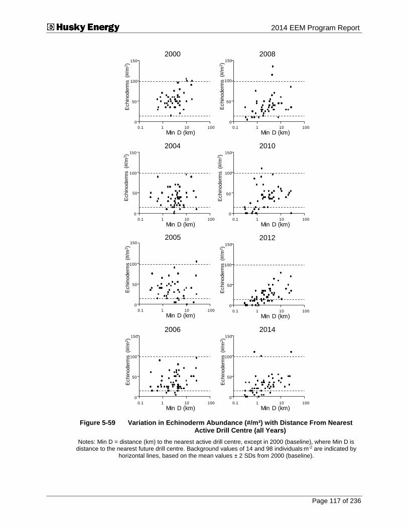
Submitted To 2014 EEM Program Report
Page 117 of 236
0.1 1 10 100
Min D (km)
0
50
100
150
Echin
oderm
s (
#/m
2)
2000
0.1 1 10 100
Min D (km)
0
50
100
150
Echin
oderm
s (
#/m
2)
2004
0.1 1 10 100
Min D (km)
0
50
100
150
Echin
oderm
s (
#/m
2)
2005
0.1 1 10 100
Min D (km)
0
50
100
150
Echin
oderm
s (
#/m
2)
2006
0.1 1 10 100
Min D (km)
0
50
100
150
Echin
oderm
s (
#/m
2)
2008
0.1 1 10 100
Min D (km)
0
50
100
150
Echin
oderm
s (
#/m
2)
2010
0.1 1 10 100
Min D (km)
0
50
100
150
Echin
oderm
s (
#/m
2)
2012
0.1 1 10 100
Min D (km)
0
50
100
150
Echin
oderm
s (
#/m
2)
2014
Figure 5-59 Variation in Echinoderm Abundance (#/m²) with Distance From Nearest Active Drill Centre (all Years)
Notes: Min D = distance (km) to the nearest active drill centre, except in 2000 (baseline), where Min D is distance to the nearest future drill centre. Background values of 14 and 98 individuals.m-2 are indicated by
horizontal lines, based on the mean values ± 2 SDs from 2000 (baseline).

Submitted To 2014 EEM Program Report
Page 118 of 236
Figure 5-60 Location of Stations with Echinoderm Abundance (#/m²) Within and Below the Baseline Range (2014)

Submitted To 2014 EEM Program Report
Page 119 of 236
Table 5-28 Repeated-measures Regression Testing for Changes in Total Benthic Biomass over Time
Trend over Time Before to After
Slope Mean Slope Mean
0.003 <0.001 0.106 0.001
Notes: - Values are probabilities. - n = 36. - The trend over Time contrast tests for trends over time since operations began (i.e., from 2004 to
2014). - The Before to After contrast tests for differences between year 2000 (baseline) and the mean in
the period including 2004 to 2014.
2000 2002 2004 2006 2008 2010 2012 2014
Year
0
500
1000
1500
2000
Bio
ma
ss (
g/m
2)
Figure 5-61 Dot Density Plot of Total Benthic Biomass by Year
Note: Background values of 367 and 1,400 g.m-2 are indicated by horizontal lines, based on the mean values ± 2 SDs from the baseline year (2000),
5.2.3.5 Richness
Number of families per station (i.e., richness) varied between 22 and 56 in 2014, which compares well to the baseline range of between 21 and 38 families. Richness was not
significantly correlated with distance to the nearest active drill centre in 2014 (s = -0.15,
p > 0.05, All stations; s = -0.17, p > 0.05, repeated-measures stations), or other years (Figure 5-62). Figures 5-63 and 5-64 provide graphical representations of the relationship between richness and distance to active drill centres. In 2014, richness was not reduced at any drill centre (Figure 5-64).

Submitted To 2014 EEM Program Report
Page 120 of 236
RM Stations
All StationsRichness
2000 2002 2004 2006 2008 2010 2012 2014
Year
-1.0
-0.5
0.0
0.5
1.0
Sp
earm
an
Ran
k
Figure 5-62 Spearman Rank Correlations with Distance from the Nearest Active Drill Centre for Taxa Richness
Notes: n = 53 for All Stations. n = 36 for Repeated-Measures (RM) Stations. Dotted lines indicate rank correlations of |0.3|, which were generally significant at p < 0.01, depending on sample size in the
given year; however, significance from specific statistical tests reported in text.

Submitted To 2014 EEM Program Report
Page 121 of 236
0.1 1 10 100
Min D (km)
0
20
40
60
Ric
hness
2000
0.1 1 10 100
Min D (km)
0
20
40
60
Ric
hness
2004
0.1 1 10 100
Min D (km)
0
20
40
60
Ric
hness
2005
0.1 1 10 100
Min D (km)
0
20
40
60
Ric
hness
2006
0.1 1 10 100
Min D (km)
0
20
40
60
Ric
hness
2008
0.1 1 10 100
Min D (km)
0
20
40
60
Ric
hness
2010
0.1 1 10 100
Min D (km)
0
20
40
60
Ric
hness
2012
0.1 1 10 100
Min D (km)
0
20
40
60
Ric
hness
2014
Figure 5-63 Variation in Taxa Richness with Distance From Nearest Active Drill Centre (all Years)
Notes: Min D = distance (km) to the nearest active drill centre, except in 2000 (baseline), where Min D is distance to the nearest future drill centre. Background number of families (22) is indicated by a horizontal
line, based on the mean values + 2 SDs using data from 2000.

Submitted To 2014 EEM Program Report
Page 122 of 236
Figure 5-64 Location of Stations with Richness Values Within and Below the Baseline Range (2014)

Submitted To 2014 EEM Program Report
Page 123 of 236
Repeated-measures regression (Table 5-29) indicated the slope of the relationship between number of families and distance from the nearest active drill centre has not varied over time during the drilling period for repeated-measures stations (p = 0.169). The relationship also has not changed significantly from before to after drilling (p = 0.084). There was a significant linear trend (increase; p < 0.001; see Figure 5-65) in number of families during the active drilling period of 2004 to 2014. However, the number of families did not differ significantly between the drilling period compared to the baseline year (p = 0.281; see Figure 5-65).
Table 5-29 Repeated-measures Regression Testing for Changes in Taxa Richness over Time
Trend over Time Before to After
Slope Mean Slope Mean
0.169 <0.001 0.084 0.281
Notes: - Values are probabilities. - n = 36. - The trend over Time contrast tests for trends over time since operations began (i.e., from 2004 to
2014). - The Before to After contrast tests for differences between year 2000 (baseline) and the mean in
the period including 2004 to 2014.
2000 2002 2004 2006 2008 2010 2012 2014
Year
0
10
20
30
40
50
60
Ric
hne
ss
Figure 5-65 Dot Density Plot of Taxa Richness by Year
Note: Background number of families is indicated by horizontal lines, based on the mean values ± 2 SDs using data from 2000.
In 2014, no observations fell below the estimated limits of the baseline range (i.e., below 21 families) (Figure 5-65). Results indicate that there has been no reduction in the number of families (richness) in the sampling area and, in fact, there has been a slight increase in richness since 2005 with the greatest increase noted from 2012 to 2014 surveys.

Submitted To 2014 EEM Program Report
Page 124 of 236
5.2.3.6 Paraonidae Abundance
Paraonidae are a family of slender burrowing polychaete worms. Their abundances have been strongly related to distance from active drill centres (Figure 5-66), with abundances
depressed near drill centres in most EEM years and in 2014 (s = 0.76, p < 0.001, All
stations; (s = 0.75, p < 0.001, repeated-measures stations). Threshold models were significant for Paraonidae abundance for all years from 2004 to 2014 (Table 5-30). Threshold distances have been somewhat variable (1.5 km in 2014 to 4.1 km in 2004) (Table 5-30). Figure 5-67 provides a graphical representation of the relationship between Paraonidae abundance and distance to active drill centres.
RM Stations
All StationsParaonidae
2000 2002 2004 2006 2008 2010 2012 2014
Year
-1.0
-0.5
0.0
0.5
1.0
Sp
earm
an
Ran
k
Figure 5-66 Spearman Rank Correlations with Distance from the Nearest Active Drill Centre for Paraonidae Abundances
Notes: n = 53 for All Stations. n = 36 for Repeated-Measures (RM) Stations. Dotted lines indicate rank correlations of |0.3|, which were generally significant at p < 0.01, depending on sample size in the
given year; however, significance from specific statistical tests reported in text.
Table 5-30 Threshold Distances Computed from Threshold Regressions on Distance from the Nearest Active Drill Centre for Paraonidae Abundance
Year Threshold Distance (km)
2004 4.1 (2.0 to 8.6)
2005 2.6 (1.5 to 4.5)
2006 2.8 (1.9 to 4.2)
2008 3.8 (2.1 to 6.9)
2010 1.6 (1.0 to 2.7)
2012 2.5 (1.5, 4.3)
2014 1.5 (0.5 to 3.0)
Note: - 95% confidence limits are provided in brackets.
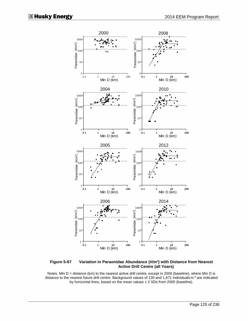
Submitted To 2014 EEM Program Report
Page 125 of 236
0.1 1 10 100
Min D (km)
1
10
100
1000
Para
onid
ae
(#/m
2)
2000
0.1 1 10 100
1
10
100
1000
2004
0.1 1 10 100
Min D (km)
Para
onid
ae
(#/m
2)
0.1 1 10 100
1
10
100
1000
2005
0.1 1 10 100
Min D (km)
Para
onid
ae
(#/m
2)
0.1 1 10 100
1
10
100
1000
2006
0.1 1 10 100
Min D (km)
Para
onid
ae
(#/m
2)
0.1 1 10 100
1
10
100
1000
0.1 1 10 100
Min D (km)
Para
onid
ae
(#/m
2)
0.1 1 10 100
1
10
100
1000
2010
0.1 1 10 100
Min D (km)P
ara
onid
ae
(#/m
2)
0.1 1 10 100
1
10
100
1000
2012
0.1 1 10 100
Min D (km)
Para
onid
ae
(#/m
2)
0.1 1 10 100
1
10
100
1000
2014
0.1 1 10 100
Min D (km)
Para
onid
ae
(#/m
2)
2008
Figure 5-67 Variation in Paraonidae Abundance (#/m²) with Distance from Nearest Active Drill Centre (all Years)
Notes: Min D = distance (km) to the nearest active drill centre, except in 2000 (baseline), where Min D is distance to the nearest future drill centre. Background values of 130 and 1,671 individuals.m-2 are indicated
by horizontal lines, based on the mean values ± 2 SDs from 2000 (baseline).

Submitted To 2014 EEM Program Report
Page 126 of 236
As indicated in Figure 5-67, the “normal range” of variation for Paraonidae abundance across the sampling area was computed from the 2000 baseline data. Values ranged from 130 and 1,671 per m² in 2000. The lower range of 130 individuals per m² was used as a “benchmark” against which to judge spatial variations in the sampling area (Figure 5-68) as well as variations over time (Figure 5-69).
Paraonidae abundances were reduced at several stations around the Central, North Amethyst and Southern Drill Centres in 2014 (Figure 5-68). Paraonidae abundances were reduced below baseline values at two stations around the Northern Drill Centre and at one station around the SWRX Drill Centre. There were approximately as many stations with Paraonidae abundance below the lower baseline range of abundance (i.e., less than 130 per m²) in 2014 (45%) as in 2012 (38%) or 2010 (40%) (Figure 5-69).
Repeated-measures regression (Table 5-31) indicated there was a significant linear trend over time in the slope of the relationship between distance and Paraonidae abundance during the period of drilling operations (increase in the slope, p < 0.001) for repeated-measures stations. There was also a difference in the slope from before to after drilling (higher slope during drilling, p < 0.001); a linear decrease over time in mean Paraonidae abundances during the drilling period (p < 0.001); and overall lower numbers of Paraonidae from before to after drilling (p < 0.001), with effects caused by the low abundances near active drill centres.
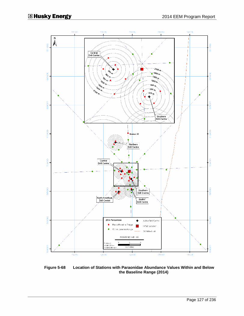
Submitted To 2014 EEM Program Report
Page 127 of 236
Figure 5-68 Location of Stations with Paraonidae Abundance Values Within and Below the Baseline Range (2014)
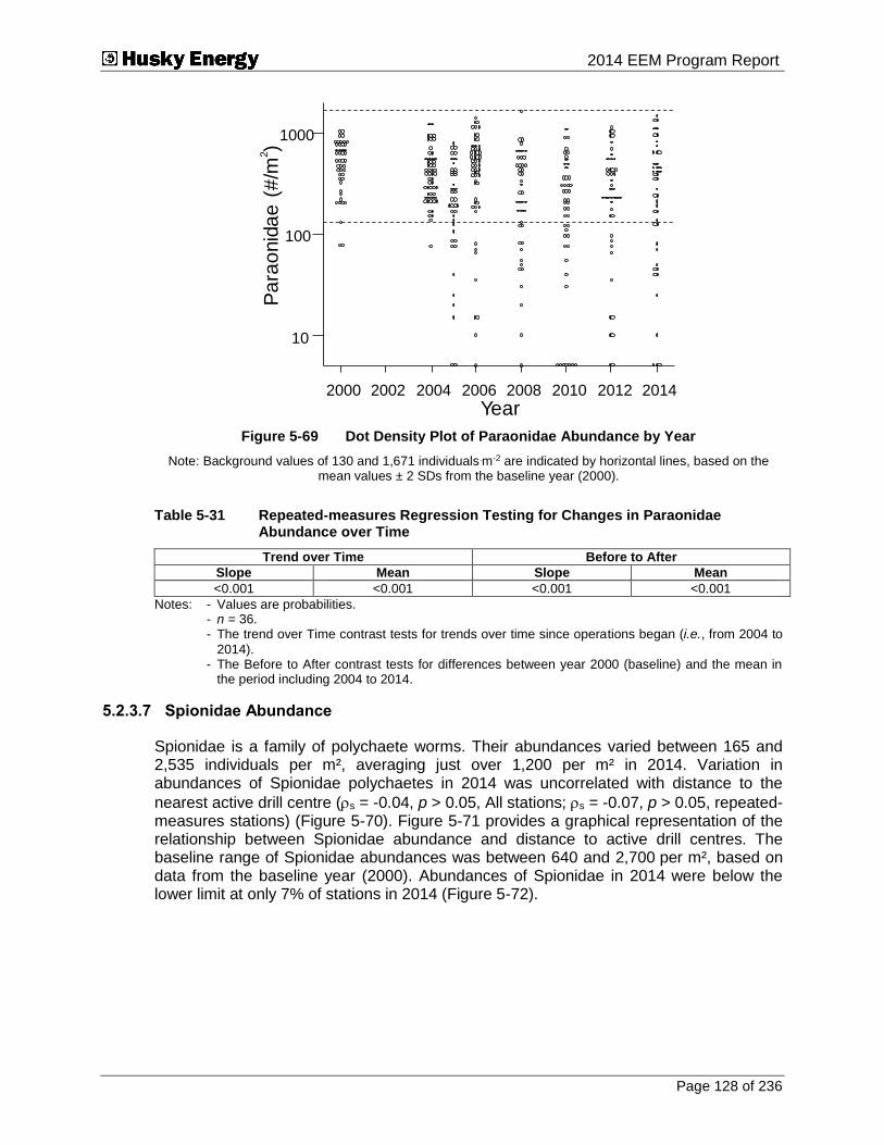
Submitted To 2014 EEM Program Report
Page 128 of 236
2000 2002 2004 2006 2008 2010 2012 2014
Year
10
100
1000
Pa
rao
nid
ae
(#
/m2)
Figure 5-69 Dot Density Plot of Paraonidae Abundance by Year
Note: Background values of 130 and 1,671 individuals.m-2 are indicated by horizontal lines, based on the mean values ± 2 SDs from the baseline year (2000).
Table 5-31 Repeated-measures Regression Testing for Changes in Paraonidae Abundance over Time
Trend over Time Before to After
Slope Mean Slope Mean
<0.001 <0.001 <0.001 <0.001
Notes: - Values are probabilities. - n = 36. - The trend over Time contrast tests for trends over time since operations began (i.e., from 2004 to
2014). - The Before to After contrast tests for differences between year 2000 (baseline) and the mean in
the period including 2004 to 2014.
5.2.3.7 Spionidae Abundance
Spionidae is a family of polychaete worms. Their abundances varied between 165 and 2,535 individuals per m², averaging just over 1,200 per m² in 2014. Variation in abundances of Spionidae polychaetes in 2014 was uncorrelated with distance to the
nearest active drill centre (s = -0.04, p > 0.05, All stations; s = -0.07, p > 0.05, repeated-measures stations) (Figure 5-70). Figure 5-71 provides a graphical representation of the relationship between Spionidae abundance and distance to active drill centres. The baseline range of Spionidae abundances was between 640 and 2,700 per m², based on data from the baseline year (2000). Abundances of Spionidae in 2014 were below the lower limit at only 7% of stations in 2014 (Figure 5-72).

Submitted To 2014 EEM Program Report
Page 129 of 236
RM Stations
All StationsSpionidae
2000 2002 2004 2006 2008 2010 2012 2014
Year
-1.0
-0.5
0.0
0.5
1.0
Sp
earm
an
Ran
k
Figure 5-70 Spearman Rank Correlations with Distance from the Nearest Active Drill Centre for Spionidae Abundances
Notes: n = 53 for All Stations. n = 36 for Repeated-Measures (RM) Stations. Dotted lines indicate rank correlations of |0.3|, which were generally significant at p < 0.01, depending on sample size in the
given year; however, significance from specific statistical tests reported in text.

Submitted To 2014 EEM Program Report
Page 130 of 236
0.1 1 10 100
Min D (km)
1
10
100
1000
Spio
nid
ae
(#/m
2)
2000
0.1 1 10 100
Min D (km)
1
10
100
1000
Spio
nid
ae
(#/m
2)
2004
0.1 1 10 100
Min D (km)
1
10
100
1000
Spio
nid
ae
(#/m
2)
2005
0.1 1 10 100
Min D (km)
1
10
100
1000
Spio
nid
ae
(#/m
2)
2006
0.1 1 10 100
Min D (km)
1
10
100
1000
Spio
nid
ae
(#/m
2)
2008
0.1 1 10 100
Min D (km)
1
10
100
1000
Spio
nid
ae
(#/m
2)
2010
0.1 1 10 100
Min D (km)
1
10
100
1000
Spio
nid
ae
(#/m
2)
2012
0.1 1 10 100
Min D (km)
1
10
100
1000
Spio
nid
ae
(#/m
2)
2014
Figure 5-71 Variation in Spionidae Abundance (#/m²) with Distance From Nearest Active Drill Centre (all Years)
Notes: Min D = distance (km) to the nearest active drill centre, except in 2000 (baseline), where Min D is distance to the nearest future drill centre. Background values of 640 and 2,700 individuals.m-2 are indicated
by horizontal lines, based on the mean values ± 2 SDs from 2000 (baseline).

Submitted To 2014 EEM Program Report
Page 131 of 236
2000 2002 2004 2006 2008 2010 2012 2014
Year
10
100
1000
Spio
nid
ae
(#
/m2)
Figure 5-72 Dot Density Plot of Spionidae Abundance by Year
Note: Background values of 640 and 2,700 individuals.m-2 are indicated by horizontal lines, based on the mean values ± 2 SDs from the baseline year (2000).
Repeated-measures regression (Table 5-32) indicated no significant change in the slope of the relationship between Spionidae abundance and distance from the nearest active drill centre over time for repeated measured stations (p = 0.093), and no difference in slope from before to after active drilling operations (p = 0.168). There was a difference in mean Spionidae abundance across the sampling area from before to after active drilling (p < 0.001) that appears to have been driven by reduced abundances in 2005, 2010 and 2012 (Figure 5-72). These same reductions combined with the relative increase in abundances in 2014 were likely the drivers of the significant difference in mean abundances observed between 2004 and 2014 (Figure 5-72).
Table 5-32 Repeated-measures Regression Testing for Changes in Spionidae Abundance over Time
Trend over Time Before to After
Slope Mean Slope Mean
0.093 0.003 0.168 <0.001
Notes: - Values are probabilities. - n = 36. - The Trend over Time contrast tests for trends over time since operations began (i.e., from 2004 to
2014). - The Before to After contrast tests for differences between year 2000 (baseline) and the mean in
the period including 2004 to 2014.
The absence of correlation between Spionidae abundances and distance to nearest active drill centres suggests no effects on Spionidae in 2014.

Submitted To 2014 EEM Program Report
Page 132 of 236
5.2.3.8 Tellinidae Abundance
Tellinidae is a family of marine bivalve molluscs. Their abundances varied between 5 and 1,245 individuals per m², with an area-wide average of approximately 500 per m² in 2014. The baseline range of Tellinidae abundances from year 2000 was between 151 and 1,303 individuals per m².. The correlation between Tellinidae abundance and distance to active drill centres was significant in 2014, 2012, 2010 and 2008 when only the repeated
stations were considered (2014: s = 0.05, p > 0.05, All stations; s = 0.53, p < 0.001, repeated-measures stations (Figure 5-73). Figures 5-74 and 5-75 provide a graphical representation of the relationship between Tellinidae abundance and distance to active drill centres.
RM Stations
All StationsTellinidae
2000 2002 2004 2006 2008 2010 2012 2014
Year
-1.0
-0.5
0.0
0.5
1.0
Sp
earm
an
Ran
k
Figure 5-73 Spearman Rank Correlations with Distance from the Nearest Active Drill Centre for Tellinidae Abundance
Notes: n = 53 for All Stations. n = 36 for Repeated-Measures (RM) Stations. Dotted lines indicate rank correlations of |0.3|, which were generally significant at p < 0.01, depending on sample size in the
given year; however, significance from specific statistical tests reported in text.
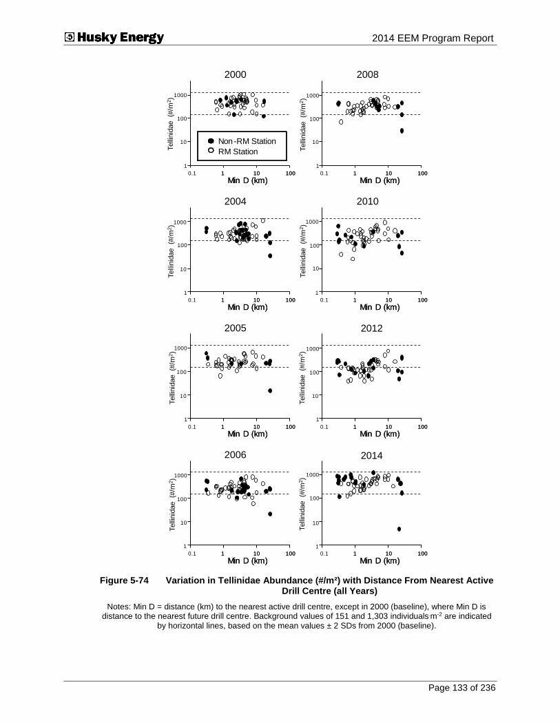
Submitted To 2014 EEM Program Report
Page 133 of 236
1 10 100
Min D (km)
1
10
100
1000
Telli
nid
ae
(#/m
2)
2000
0.1 1 10 100
Min D (km)
1 10 100
Min D (km)
1
10
100
1000
Telli
nid
ae
(#/m
2)
2004
0.1 1 10 100
Min D (km)
0.1 1 10 100
Min D (km)
1
10
100
1000
Telli
nid
ae
(#/m
2)
1 10 100
Min D (km)
2005
0.1 1 10 100
Min D (km)
1
10
100
1000
Telli
nid
ae
(#/m
2)
1 10 100
Min D (km)
2006
0.1 1 10 100
Min D (km)
1
100
1000
Telli
nid
ae
(#/m
2)
1 10 100
Min D (km)
10
2008
0.1 1 10 100
Min D (km)
1
10
100
1000
Telli
nid
ae
(#/m
2)
1 10 100
Min D (km)
2010
0.1 1 10 100
Min D (km)
1
10
100
1000
Telli
nid
ae
(#/m
2)
1 10 100
Min D (km)
1 10 100
Min D (km)
1
100
1000
Telli
nid
ae
(#/m
2)
0.1 1 10 100
Min D (km)
10
Non-RM Station
RM Station
2012
2014
Figure 5-74 Variation in Tellinidae Abundance (#/m²) with Distance From Nearest Active Drill Centre (all Years)
Notes: Min D = distance (km) to the nearest active drill centre, except in 2000 (baseline), where Min D is distance to the nearest future drill centre. Background values of 151 and 1,303 individuals.m-2 are indicated
by horizontal lines, based on the mean values ± 2 SDs from 2000 (baseline).

Submitted To 2014 EEM Program Report
Page 134 of 236
Figure 5-75 Location of Stations with Tellinidae Abundance Values Within and Below the Baseline Range (2014)

Submitted To 2014 EEM Program Report
Page 135 of 236
Repeated-measures regression (Table 5-33) indicated that the slope of the relationship between Tellinidae abundance and distance to the nearest active drill centre was different between drilling and pre-drilling years for repeated-measures stations (p = 0.005), yet the slope of the relationship did not significantly vary during drilling years (p = 0.171; Figure 5-73). There was no tendency for mean numbers of Tellinidae to vary over time during drilling years (p = 0.561) but a significant difference was noted from baseline to drilling periods (p < 0.001; although numbers in 2014 are comparable to numbers during baseline; Figure 5-76).
Table 5-33 Repeated-measures Regression Testing for Changes in Tellinidae Abundance over Time
Trend over Time Before to After
Slope Mean Slope Mean
0.171 0.561 0.005 <0.001
Notes: - Values are probabilities. - n = 36. - The trend over Time contrast tests for trends over time since operations began (i.e., from 2004 to
2014). - The Before to After contrast tests for differences between year 2000 (baseline) and the mean in
the period including 2004 to 2014.
2000 2002 2004 2006 2008 2010 2012 2014
Year
10
100
1000
Te
llinid
ae
(#
/m2)
Figure 5-76 Dot Density Plot of Tellinidae Abundance by Year
Note: Background values of 151 and 1,303 individuals.m-2 are indicated by horizontal lines, based on the mean values ± 2 SDs from 2000 (baseline).
The repeated-measures regression results for before to after active drilling operations support the simpler Spearman rank correlation analysis and suggest that there was a relationship between abundance of Tellinidae bivalves and distance to the nearest active drill centre for repeated-measures stations. The scatterplots in Figure 5-74 illustrate that when considering only the stations included in the repeated-measures regression, abundances of Tellinidae were somewhat lower nearer active drill centres in drilling

Submitted To 2014 EEM Program Report
Page 136 of 236
years. However, the stations included in the repeated-measures regression do not include the stations nearest and furthest from drill centres.
Only 6% (n = 3) of all stations had Tellinidae abundances in 2014 that were below the lower baseline value of 151 per m² (Figure 5-76). The absence of strong correlation of Tellinidae abundances with distance to nearest active drill centres for all data suggests that the observed variations are not solely related to proximity to White Rose operations.
5.2.3.9 Amphipoda Abundance
Amphipoda is shrimp-like family of crustaceans. Their abundances varied between 5 and 365 individuals per m², with an area-wide average of approximately 90 per m² in 2014. The range of amphipod abundances from baseline (year 2000) was between 44 and 313 individuals per m². In 2014 and when all stations were considered, amphipod abundance was not correlated with distance to nearest active drill centre. However, amphipod abundance at repeated-measures stations was significantly inversely
correlated with distance to nearest active drill centre (s = -0.21, p > 0.05, All stations;
s = -0.51, p = 0.001, repeated-measures stations) indicating higher amphipod abundance near drill centres; Figure 5-77). Figure 5-78 provides a graphical representation of the relationship between amphipod abundance and distance to active drill centres; and shows that the relationship between amphipod abundance at repeated-measures stations in 2014 was similar to the relationship noted in baseline for those stations (also compare Spearman rank correlations in Figure 5-77).
RM Stations
All StationsAmphipoda
2000 2002 2004 2006 2008 2010 2012 2014
Year
-1.0
-0.5
0.0
0.5
1.0
Sp
earm
an
Ran
k
Figure 5-77 Spearman Rank Correlations with Distance from the Nearest Active Drill Centre for Amphipoda Abundance
Notes: n = 53 for All Stations. n = 36 for Repeated-Measures (RM) Stations. Dotted lines indicate rank correlations of |0.3|, which were generally significant at p < 0.01, depending on sample size in the
given year; however, significance from specific statistical tests reported in text.

Submitted To 2014 EEM Program Report
Page 137 of 236
Non-RM Station
RM Station
0.1 1 10 100
Min D (km)
10
100
1000
Am
phip
oda
(#/m
2)
2000
0.1 1 10 100
Min D (km)
1
0.1 1 10 100
Min D (km)
1
10
100
1000
Am
phip
oda
(#/m
2)
2004
0.1 1 10 100
Min D (km)
0.1 1 10 100
Min D (km)
1
10
100
1000
Am
phip
oda
(#/m
2)
0.1 1 10 100
Min D (km)
2005
0.1 1 10 100
Min D (km)
1
10
100
1000
Am
phip
oda
(#/m
2)
0.1 1 10 100
Min D (km)
2006
0.1 1 10 100
Min D (km)
1
10
100
1000
Am
phip
oda
(#/m
2)
0.1 1 10 100
Min D (km)
2008
0.1 1 10 100
Min D (km)
1
10
100
1000
Am
phip
oda
(#/m
2)
0.1 1 10 100
Min D (km)
2010
0.1 1 10 100
Min D (km)
1
10
100
1000
Am
phip
oda
(#/m
2)
0.1 1 10 100
Min D (km)
0.1 1 10 100
Min D (km)
1
10
100
1000
Am
phip
oda
(#/m
2)
0.1 1 10 100
Min D (km)
2012
2014
Figure 5-78 Variation in Amphipoda Abundance (#/m²) with Distance From Nearest Active Drill Centre (all Years)
Notes: Min D = distance (km) to the nearest active drill centre, except in 2000 (baseline), where Min D is distance to the nearest future drill centre. Background values of 44 and 313 individuals.m-2 are indicated by
horizontal lines, based on the mean values ± 2 SDs from 2000 (baseline).
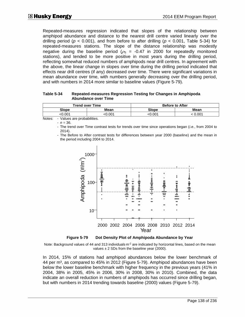
Submitted To 2014 EEM Program Report
Page 138 of 236
Repeated-measures regression indicated that slopes of the relationship between amphipod abundance and distance to the nearest drill centre varied linearly over the drilling period (p < 0.001), and from before to after drilling (p < 0.001, Table 5-34) for repeated-measures stations. The slope of the distance relationship was modestly
negative during the baseline period (S = -0.47 in 2000 for repeatedly monitored stations), and tended to be more positive in most years during the drilling period, reflecting somewhat reduced numbers of amphipods near drill centres. In agreement with the above, the linear change in slopes over time during the drilling period indicated that effects near drill centres (if any) decreased over time. There were significant variations in mean abundance over time, with numbers generally decreasing over the drilling period, and with numbers in 2014 more similar to baseline values (Figure 5-79).
Table 5-34 Repeated-measures Regression Testing for Changes in Amphipoda Abundance over Time
Trend over Time Before to After
Slope Mean Slope Mean
<0.001 <0.001 <0.001 < 0.001
Notes: - Values are probabilities. - n = 36. - The trend over Time contrast tests for trends over time since operations began (i.e., from 2004 to
2014). - The Before to After contrast tests for differences between year 2000 (baseline) and the mean in
the period including 2004 to 2014.
2000 2002 2004 2006 2008 2010 2012 2014
Year
10
100
1000
Am
phip
oda
(#/m
2)
Figure 5-79 Dot Density Plot of Amphipoda Abundance by Year
Note: Background values of 44 and 313 individuals.m-2 are indicated by horizontal lines, based on the mean values ± 2 SDs from the baseline year (2000).
In 2014, 15% of stations had amphipod abundances below the lower benchmark of 44 per m³, as compared to 45% in 2012 (Figure 5-79). Amphipod abundances have been below the lower baseline benchmark with higher frequency in the previous years (41% in 2004, 38% in 2005, 45% in 2006, 30% in 2008, 30% in 2010). Combined, the data indicate an overall reduction in numbers of amphipods has occurred since drilling began, but with numbers in 2014 trending towards baseline (2000) values (Figure 5-79).

Submitted To 2014 EEM Program Report
Page 139 of 236
5.3 Summary of Results
5.3.1 Whole-Field Response
Hydrocarbons in the >C10-C21 range found in oil-based drill muds and barium in sediments were clearly influenced by drilling operations in 2014, with concentrations elevated up to estimated threshold distances of 5.8 km and 1.0 km from the nearest active drill centre, respectively. Significant threshold values (i.e., the distance at which values return to background values) have been detected in all sampling years for >C10-C21 hydrocarbons and barium since drilling began. The threshold for >C10-C21 hydrocarbons has varied from 3.6 km (in 2010 and 2012) to 10.4 km (in 2008). The threshold distance for hydrocarbons in 2014 was 5.8 km, which is greater than the 3.6 km and less than the 10.4 km distances noted in the 2010, 2012 and 2008 EEM programs, respectively. The threshold for barium varied from 1 km (in 2012 and 2014) to 3.6 km (in 2005).
Sediment fines content and lead concentration were elevated near drill centres in 2014, with estimated threshold distances of 0.7 km, and 1 km, respectively. Thresholds could not be estimated for fines in previous years because there was no clear cut off distance between enriched stations and stations with background levels of fines. Thresholds for lead have varied from 1.5 km (in 2006) to 0.6 km (in 2012 and 2014).
Other sediment variables (TOC, ammonia, sulphide, sulphur and redox) showed increased levels in the immediate vicinity of drill centres in 2014, but threshold distances could not be estimated. For TOC, sulphide, and sulphur significant bivariate regressions (r2 = 0.286 to 0.519) showed decreasing concentrations with distance from nearest active drill centre. Redox potential also significantly increased with distance from the nearest active drill centre (r2 = 0.485).
For ammonia, analysis of trends over time (i.e., repeated-measured regression) indicated that there was no change in the relationship between ammonia and distance from drill centres over time, and overall ammonia levels have decreased over time; with all ammonia levels in 2014 below the background range. Therefore, the 2014 result does not strongly indicate project-related alterations.
Strontium concentrations were not correlated with distance to drill centres in 2014; but have been in previous years, with thresholds significant in 2006 (1.2 km), 2008 (1.6 km) and 2012 (0.6 km). There also was indication from analysis of trend over time (i.e., repeated-measures regression) that there has been a change between baseline and EEM years, with strontium higher near drill centres in EEM years. These data suggest that project-related alterations on sediment strontium concentrations have decreased over time.
There was no evidence of project-related alterations on sediment gravel content and overall metals concentration (metals PC1).
Sediments were generally non-toxic in 2014. Three samples were toxic to bacterial luminescence. Toxicity occurred in samples collected at stations 19, N1 and N2. Station 19 is a reference station and is located 22 km from the nearest drill centre. Stations N1 and N2 are located 2.2 and 1.5 km from the Northern Drill Centre, respectively. A single
Submitted To 2014 EEM Program Report
Page 140 of 236
sample was toxic to bacterial luminescence in 2010. No toxic response was noted in other years.
Two samples were toxic to laboratory amphipods in 2014 as compared to the site Reference sediment. Otherwise amphipod survival was generally greater than 80%. In 2014, the sediment sample from station C1 located 1.1 km from the Centre Drill Centre was toxic as well as the sample from station 16, located 5.59 km from the North Amethyst Drill Centre. Potential explanatory variables collected at this station (redox potential, ammonia, sediment particle size, other metal concentrations) did not suggest a cause for this toxic response at station C1. Amphipod percent survival was uncorrelated with sediment chemical or physical characteristics (including chemical characteristics influenced by project activity).
As in previous years, there was evidence of project effects on total benthic abundances and biomass; there was no evidence of effects on richness in 2014. For individual taxa, there was evidence of project effects on Paraonidae, little evidence of project effects on Tellinidae and no evidence of project effects on Spionidae and Amphipoda.
Total benthic abundances, benthic biomass and abundances of Paraonidae were correlated to concentrations of >C10-C21 hydrocarbons and barium. Total abundances and biomass, and abundances of Paraonidae were lower in sediments with high concentrations of barium and >C10-C21 hydrocarbons. Higher concentrations of sulphur also co-occurred with lower biomass and lower abundances of Paraonidae. In addition, Paraonidae abundance was negatively correlated with concentrations of lead and strontium. Paraonidae abundance has been strongly related to distance from active drill centres, with threshold distances significant in every EEM year. Threshold distances have varied from 1.5 (in 2014) to 4.1 km (in 2004).
As in previous years, the relationship between total benthic abundance and distance to active drill centres was relatively weak, with no threshold distance for effects. Total abundance ranged from approximately 1,050 to 5,920 organisms/m² near active drill centres. The range at the most distant stations (more than 10 km from drill centres) was 2,230 to 6,215 organisms/m².
Total biomass varied from approximately 4 to 1,100 g/m² near active drill centres to approximately 230 to 1,400 g/m² at the most distant stations (more than 10 km from drill centres). The relationship between total biomass and distance from active drill centres was significant in 2014, with a threshold distance for effects of approximately 5.5 km (range: 1.5 to 20.1 km). The relationship between total abundance and distance from drill centres has increased in strength since 2006. Additional analyses indicated that reductions in total biomass were associated with reductions in the numbers of larger echinoderms (mainly E. parma) near active drill centres.
Analysis results for Tellinidae differed between stations repeatedly sampled since baseline (i.e., repeated-measures stations) and all stations currently sampled, with analysis on repeated-measures station indicating a potential effect. Tellinidae abundances were reduced to levels below the baseline range at one station around the Central Drill Centre and at one station around the Southern Drill Centre. However, Tellinadae abundance was also reduced at a station 22 km from the nearest active drill centre. Overall, evidence of project effects on Tellinidae is weak.

Submitted To 2014 EEM Program Report
Page 141 of 236
5.3.2 Effects of Individual Drill Centres
Maps of response variables outside the baseline (2000) or background (>10 km from nearest active drill centre) range were used to qualitatively assess the spatial distribution of effects around individual drill centres, with a focus on benthic invertebrate responses.
In general, project effects were more pronounced around the North Amethyst, Southern and Central Drill Centres in 2014.
Total abundance in 2014 was reduced below the baseline range at two stations within 0.9 km of the Central Drill Centre, and at one station within 1.8 km of the Central Drill Centre.
Total benthic biomass in 2014 was below the baseline range at a number of stations around the Central, North Amethyst, Southern and Northern Drill Centres. Stations with reduced biomass extended to: approximately 1.8 km around the Central and Southern Drill Centres; approximately 0.9 km around the North Amethyst Drill Centre; and approximately 2.1 km around the Northern Drill Centre. The estimated spatial extent of effects from threshold models (5.5 km; Section 5.1.1) appears to be driven by the reduction in echinoderm biomass near drill centres. Paraonidae abundances in 2014 were also reduced below the baseline range at a number of stations around drill centres. Abundances were reduced to: approximately 1.8 km around the Central Drill Centre; approximately 0.9 km around the North Amethyst and Southern Drill Centres; 0.3 km (at only one station) around the SWRX Drill Centre; and approximately 0.6 km around the Northern Drill Centre. Therefore, a zone of effects of 1 to 2 km also seems appropriate for Paraonidae. In 2014, the threshold distance of 1.5 km generally agrees with the estimate of the zone of effects from examination of the maps; likely because the spatial extent of effects on Paraonidae is less extensive in 2014, resulting in reduced overlap in effects among drill centres.
As noted above, evidence of effects on Tellinidae abundance was weak in 2014. Abundances were reduced to less than the baseline range at one station located 0.3 km the Central Drill Centre and at one station located 0.6 km from the Southern Drill Centre.
Overall, 2014 data suggest that the majority of effects on benthos, excepting total biomass, are limited to within 2 km of drill centres.
In terms of magnitude of effect in 2014, and examining only the stations nearest the drill centres, mean barium and >C10-C21 hydrocarbon concentrations were highest around the North Amethyst, Southern and Central Drill Centres and mean concentrations were lowest around the SWRX Drill Centre (Table 5-35). Total benthic invertebrate abundance was reduced to less than 75% of the baseline range at one station (station C5) around the Central Drill Centre. Biomass was lowest at the Central Drill Centre overall, predominantly because of one extreme low value (4 g/m²) at station C5. Otherwise, there were more stations with benthic invertebrate biomass values less than 75% of the baseline range around North Amethyst and Southern Drill Centres. Paraonidae abundances were lowest at the North Amethyst Drill Centre, with frequent reductions also occurring at the Southern Drill Centre across the sampling years.

Submitted To 2014 EEM Program Report
Page 142 of 236
Table 5-35 Values at Drill Centre Stations for Selected Variables
Station
Distance to Drill Centre (km)
Barium (mg/kg)
>C10-C21 (mg/kg)
Fines (%)
Abundance (#/m²)
Biomass (g/m²)
Richness Paraonidae
(#/m²)
Central Drill Centre
C5 0.33 1000 92 1.73 1050 4 22 0
C3 0.74 340 17 1.10 1860 178 41 5
C2 0.83 430 18 1.28 3820 481 40 5
C4 0.92 200 1 0.97 2690 281 39 80
C1 1.14 200 5 1.10 2905 459 35 45
Mean
434 27 1.24 2465 281 35 27
Range
200 to 1000 1 to 92 0.97 to
1.73 1050 to 3820 4 to 481 22 to 41 0 to 80
Northern Drill Centre
N4 0.3 740 8 1.26 3445 385 38 45
N3 0.63 560 21 1.00 2760 202 33 5
N2 1.49 150 1 1.10 3280 349 31 470
N1 2.18 160 < 0.3 1.00 3805 263 29 460
Mean
403 8 1.09 3323 300 33 245
Range
150 to 740 < 0.3 to 21 1.00 to
1.26 2760 to 3805 202 to 385 29 to 38 5 to 470
North Amethyst Drill Centre
NA1 0.29 1000 89 1.87 2985 208 35 0
NA2 0.5 470 28 1.58 3285 145 37 0
NA3 0.76 170 3 1.11 2490 1133 33 40
NA4 1 200 2 1.12 3240 218 33 50
Mean
460 30 1.42 3000 426 35 23
Range
200 to 1000 2 to 89 1.11 to
1.87 2490 to 3285 145 to 1133 33 to 37 0 to 50
Southern Drill Centre
S5 0.31 1300 120 2.16 4810 195 41 0
S1 0.6 140 1 1.29 2870 46 40 0
S2 0.83 240 4 1.37 4700 223 47 0
S4 0.92 210 2 1.2 1940 257 37 70
S3 1.4 190 2 1.24 5920 465 50 350
Mean
416 26 1.45 4048 237 43 84
Range
140 to 1300 1 to 120 1.20 to
2.16 2870 to 5920 46 to 465 37 to 50 0 to 350
SWRX Drill Centre
SWRX1 0.32 160 2 1.28 3350 1043 41 125
SWRX2 0.44 200 1 1.22 3360 449 42 130
SWRX3 0.74 200 4 1.22 4120 713 35 175
SWRX4 1.06 160 1 1.1 3470 406 35 645
Mean
180 2 1.20 3575 653 38 269
Range
160 to 200 1 to 4 1.10 to
1.28 3350 to 4120 449 to 1043 35 to 41 125 to 645
Notes: - Stations N1 and N2 were also toxic to bacterial luminescence while station C1 was toxic to laboratory amphipods.
- Shading indicates values 75% below the baseline range for benthic invertebrates. Based on this threshold, cut-off levels for total abundance, biomass and Paraonidae abundance are 1,413 #/m², 275 g/m² and 97 #/m², respectively.

Submitted To 2014 EEM Program Report
Page 143 of 236
6.0 Commercial Fish Component
6.1 Methods
6.1.1 Field Collection
American plaice (plaice) and snow crab (crab) were collected on-board the commercial trawler M/V Kinguk between June 26 and June 28, 2014. Collection dates for the baseline program and subsequent EEM programs, and tests performed on collected specimens, are shown in Table 6-1.
Table 6-1 Field Trip Dates
Trip Collections/Tests Date
2000 Baseline Program
Study Area crab for body burden analysis; Study and Reference Area plaice for body burden and taste analysis; Study Area plaice for health analysis.
July 4 to July 10, 2000
2002 Baseline Program
Reference Area crab for body burden analysis; Study and Reference Area crab for taste analysis; Reference Area plaice for health analysis.
June 24 to July 10, 2002
2004 EEM Program
Study and Reference Area plaice and crab for body burden and taste analysis. Study and Reference Area plaice for health analysis.
July 10 to July 18, 2004
2005 EEM Program
Study and Reference Area plaice and crab for body burden and taste analysis. Study and Reference Area plaice for health analysis.
July 8 to July 13, 2005
2006 EEM Program
Study and Reference Area plaice and crab for body burden and taste analysis. Study and Reference Area plaice for health analysis.
July 11 to July 20, 2006
2008 EEM Program
Study and Reference Area plaice and crab for body burden and taste analysis. Study and Reference Area plaice for health analysis.
May 26 to June 2, 2008
2010 EEM Program
Study and Reference Area plaice and crab for body burden and taste analysis. Study and Reference Area plaice for health analysis.
July 2 to July 5, 2010
2012 EEM Program
Study and Reference Area plaice and crab for body burden and taste analysis. Study and Reference Area plaice for health analysis.
July 8 to July 10, 2012
2014 EEM Program
Study and Reference Area plaice and crab for body burden and taste analysis. Study and Reference Area plaice for health analysis.
June 26 to June 28, 2014
Notes: - Since the location of Reference Areas sampled from 2004 to 2014 differs from locations sampled in 2000 and 2002, data from Reference Areas collected during baseline cannot be compared to EEM Reference Area data (see Husky Energy 2004 for details).
Details on the collection and processing of 2000, 2002, 2004, 2005, 2006, 2008, 2010 and 2012 samples are presented in Husky Energy (2001, 2003, 2005, 2006, 2007, 2009, 2011, 2013). Sampling for the 2014 program was conducted under an experimental fishing license (NL-2578-14), which included Condition 13 (authorization to engage in activities that may incidentally kill, harm, harass, capture or take the following species listed on Schedule 1 of the Species at Risk Act (northern wolffish, spotted wolffish, Atlantic wolffish or leatherback turtle)) issued by Fisheries and Oceans Canada (DFO). A total of 100 plaice and 82 crab from the White Rose Study Area were retained from 10 transects for analysis in 2014. A total of 120 plaice and 105 crab were retained from 12 transects in Reference Areas. Plaice and crab that were not retained, as well as non-Species at Risk Act by-catch, were released with as little damage as possible. No species at risk were reported from any of the trawls. Location of transects are provided in Figure 6-1 and Appendix C-113.
13 In previous years, trawl by-catch was also provided in this Appendix. However, because a commercial trawl, rather than DFO’s Campelen trawl, has been used since 2010, by-catch is now minimal and not comparable to by-catch obtained in previous years.

Submitted To 2014 EEM Program Report
Page 144 of 236
Figure 6-1 2014 EEM Program Transect Locations
Submitted To 2014 EEM Program Report
Page 145 of 236
Preliminary processing of samples was done on-board the vessel. Plaice and crab that had suffered obvious trawl damage were discarded. Only plaice larger than 300 mm in length and crab larger than 60 mm in carapace width were retained for analysis. Tissue samples, top fillet for plaice and left legs for crab, were frozen at -20°C for taste analysis. Bottom fillets and liver (left half only) for plaice and right legs for crab were frozen at -20°C for body burden analysis. Blood, gill, liver (right half), heart, spleen, gonad, kidney and otolith samples from plaice were preserved for fish health analysis (see below). Additional measurements on plaice included fish length, weight (whole and gutted), sex and maturity stage, liver weight and gonad weight. For crab, measurements included carapace width, shell condition (see Appendix C-1 for shell condition indices), sex and chela height.
The following procedures were used for collection of fish health indicator samples. Each fish was assessed visually for any parasites and/or abnormalities on the skin and fins or on internal organs (liver, gonads, digestive tract, musculature and spleen) under the general framework of Autopsy-Based Condition Assessment described by Goede and Barton (1990). Fish were dissected and sex and maturity stage were determined by visual examination according to procedures used by DFO in the Newfoundland Region.
Approximately 0.5 to 1.0 ml of blood was drawn from a dorsal vessel near the tail with a disposable syringe previously coated with an anticoagulant, dispensed carefully into a labelled tube containing an anticoagulant and gently mixed. Two blood smears were prepared for each fish within one hour of blood collection according to standard haematological methods (Platt 1969). The entire liver was excised and bisected. A 4 to 5 mm-thick slice was cut from the centre portion of the right half of the liver (along the longitudinal axis) and placed in Dietrich’s fixative for histological processing. The remainder of the right half was frozen on dry ice until return to port, when it was placed in a -65°C freezer for MFO analysis. The first gill arch on the right side/top side of the fish was removed and placed in 10% buffered formalin for histological processing. A pair of otoliths was removed for ageing. Throughout the dissection process, any internal parasites and/or abnormal tissues were recorded and preserved in Deitrich's fixative for subsequent identification.
6.1.1.1 Sampling Quality Assurance/Quality Control
The following sampling QA/QC protocols were implemented. For each transect, the top deck of the survey vessel was washed with degreaser then flushed with seawater. The fishing deck and chute leading to the processing facilities were flushed continuously during the survey. All measuring instruments and work surfaces were washed with mild soap and water, disinfected with isopropyl alcohol, then rinsed with distilled water prior to the start of each transect. Sampling personnel wore new latex gloves for each transect. Processed samples were transferred to a -20°C freezer within one hour of collection where applicable.
6.1.2 Laboratory Analysis
6.1.2.1 Allocation of Samples
Plaice were used for body burden analysis, taste tests and fish health assessment. Plaice bottom fillets and liver tissues from each transect were composited to generate 10 individual body burden samples for fillet and liver for the Study Area and three composites for each of the Reference Areas, for a total of 12 composites for the

Submitted To 2014 EEM Program Report
Page 146 of 236
Reference Areas. When sufficient tissue was available, tissue from individual fish was archived for subsequent body burden on individuals if warranted by results of health analyses. Top fillets from a subset of fish used in body burden analysis were used in taste analysis. In this test, fish fillets selected from the Study Area and the Reference Areas were allocated to the triangle test and the hedonic scaling test (see Section 6.1.2.3 for details on taste tests) and then randomly assigned to panelists. Fish health analyses, by design, were conducted on individual fish rather than composite or randomly assigned samples (see Table 6-2).
Table 6-2 Plaice Selected for Body Burden, Taste and Health Analyses (2014)
Transect No.
Area No. of Fish Retained
Body Burden Composites
(Bottom Fillet, or Liver)
Taste Test (wt. (g) of
Top Fillets)
Fish Health (No. of Fish)
WR7 Study Area 10 WR7 (6 fish) 722.5 6
WR8 Study Area 10 WR8 (6 fish) 730.1 6
WR9 Study Area 10 WR9 (10 fish) 715.8 6
WR10 Study Area 10 WR10 (6 fish) 727.4 6
WR11 Study Area 10 WR11(10 fish) 725.5 6
WR12 Study Area 10 WR12 (10 fish) 718.2 6
WR13 Study Area 10 WR13 (10 fish) 726.8 6
WR14 Study Area 10 WR14 (10 fish) 729.5 6
WR15 Study Area 10 WR15 (6 fish) 728.2 6
WR16 Study Area 10 WR16 (6 fish) 708.3 6
Study Area Total
100 10 7,232.3 60
WR1 Reference Area 2 10 WR1 (10 fish) 733.1 10
WR2 Reference Area 2 10 WR2 (10 fish) 723.2 10
WR3 Reference Area 2 10 WR3 (10 fish) 699.2 10
WR4 Reference Area 3 10 WR4 (10 fish) 732.9 10
WR5 Reference Area 3 10 WR5 (10 fish) 723.4 10
WR6 Reference Area 3 10 WR6 (10 fish) 729.8 10
WR17 Reference Area 4 10 WR17 (10 fish) 724.2 10
WR18 Reference Area 4 10 WR18 (10 fish) 708.4 10
WR19 Reference Area 4 10 WR19 (10 fish) 724.8 10
WR20 Reference Area 1 10 WR20 (10 fish) 721.1 10
WR21 Reference Area 1 10 WR21 (10 fish) 727.4 10
WR22 Reference Area 1 10 WR22 (10 fish) 701.5 10
Reference Area Total
120 12 8,649.0 120
Note: - Additional fish were required for body burden composites for transects WR9, WR11, WR12, WR13 and WR14 to obtain necessary liver mass to perform all chemistry analyses.
- A much as feasible, tissue weights for taste tests were selected to generate relatively constant weights over all composites within the Study Area or over each of the Reference Areas.
Crab were used for body burden and taste analyses. Only hard shell crab were tested. From each transect, tissue from right legs was composited to generate 10 body burden samples for the Study Area and three composite samples for each of the four Reference Areas, for a total of 12 composite samples for the Reference Areas (see Table 6-3). Left leg tissue was used in taste analysis. In this test, leg tissue selected from the Study Area and the Reference Areas was allocated to the triangle test and the hedonic scaling test and then randomly assigned to panelists (see Section 6.1.2.3 for details on taste tests).

Submitted To 2014 EEM Program Report
Page 147 of 236
Table 6-3 Crab Selected for Body Burden and Taste Analysis (2014)
Transect No. Area No. of Crab
Body Burden Composites (Right Legs)
Taste Tests (wt. (g) of Crab,
Left Legs)
WR7 Study Area 7 WR7-crab (7 crab) 672.3
WR8 Study Area 6 WR8-crab (6 crab) 663.1
WR9 Study Area 6 WR9-crab (6 crab) 658.2
WR10 Study Area 3 WR10-crab (3 crab) 583.4
WR11 Study Area 12 WR11-crab (12 crab) 655.2
WR12 Study Area 12 WR12-crab (12 crab) 660.1
WR13 Study Area 12 WR13-crab (12 crab) 653.4
WR14 Study Area 12 WR14-crab (12 crab) 648.9
WR15 Study Area 6 WR15-crab (6 crab) 660.1
WR16 Study Area 6 WR16-crab (6 crab) 655.7
Study Area Total 82 10 6,510.4
WR1 Reference Area 2 11 WR1-crab (11 crab) 610.2
WR2 Reference Area 2 12 WR2-crab (12 crab) 605.2
WR3 Reference Area 2 12 WR3-crab (12 crab) 612.6
WR4 Reference Area 3 4 WR4-crab (4 crab) 540.2
WR5 Reference Area 3 6 WR5-crab (6 crab) 604.9
WR6 Reference Area 3 24 WR6-crab (24 crab) 613.0
WR17 Reference Area 4 6 WR17-crab (6 crab) 612.8
WR18 Reference Area 4 6 WR18-crab (6 crab) 622.1
WR19 Reference Area 4 6 WR19-crab (6 crab) 607.6
WR20 Reference Area 1 6 WR20-crab (6 crab) 604.7
WR21 Reference Area 1 6 WR21-crab (6 crab) 612.3
WR22 Reference Area 1 6 WR22-crab (6 crab) 599.6
Reference Area Total 105 12 7,245.2
Note: - A much as feasible, tissue weights for taste tests were selected to generate relatively constant weights over all composites within the Study Area or over each of the Reference Areas.
6.1.2.2 Body Burden
Samples of plaice fillet and liver as well as crab legs were delivered frozen to petroforma inc., an analytical and toxicology laboratory in St. John's, Newfoundland and Labrador, and processed for the variables listed in Table 6-4. Analytical methods for these tests are provided in Appendix C-2.
Table 6-4 Body Burden Variables (2000, 2002, 2004, 2005, 2006, 2008, 2010, 2012 and 2014)
Variables Method
Laboratory Detection Limits
Units 2000 2002
2004 & 2005
2006 2008, 2010
& 2012
2014
Hydrocarbons
>C10-C21 GC/FID 15 15 15 15 15 15 mg/kg
>C21-C32 GC/FID 15 15 15 15 15 15 mg/kg
PAHs
1-Chloronaphthalene GC/MS NA NA 0.05 0.05 0.05 0.05 mg/kg
2-Chloronaphthalene GC/MS NA NA 0.05 0.05 0.05 0.05 mg/kg
1-Methylnaphthalene GC/MS 0.05 0.05 0.05 0.05 0.05 0.05 mg/kg
2-Methylnaphthalene GC/MS 0.05 0.05 0.05 0.05 0.05 0.05 mg/kg
Acenaphthene GC/MS 0.05 0.05 0.05 0.05 0.05 0.05 mg/kg
Acenaphthylene GC/MS 0.05 0.05 0.05 0.05 0.05 0.05 mg/kg
Anthracene GC/MS 0.05 0.05 0.05 0.05 0.05 0.05 mg/kg
Benz[a]anthracene GC/MS 0.05 0.05 0.05 0.05 0.05 0.05 mg/kg
Benzo[a]pyrene GC/MS 0.05 0.05 0.05 0.05 0.05 0.05 mg/kg
Benzo[b]fluoranthene GC/MS 0.05 0.05 0.05 0.05 0.05 0.05 mg/kg
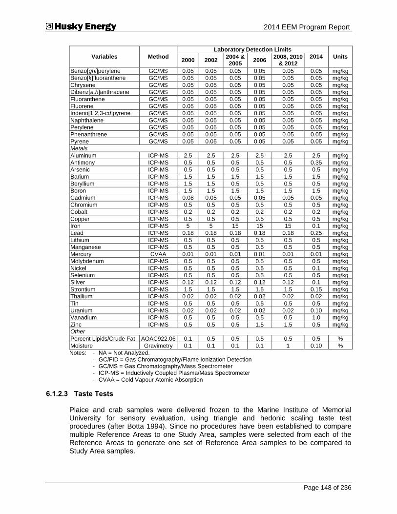
Submitted To 2014 EEM Program Report
Page 148 of 236
Variables Method
Laboratory Detection Limits
Units 2000 2002
2004 & 2005
2006 2008, 2010
& 2012
2014
Benzo[ghi]perylene GC/MS 0.05 0.05 0.05 0.05 0.05 0.05 mg/kg
Benzo[k]fluoranthene GC/MS 0.05 0.05 0.05 0.05 0.05 0.05 mg/kg
Chrysene GC/MS 0.05 0.05 0.05 0.05 0.05 0.05 mg/kg
Dibenz[a,h]anthracene GC/MS 0.05 0.05 0.05 0.05 0.05 0.05 mg/kg
Fluoranthene GC/MS 0.05 0.05 0.05 0.05 0.05 0.05 mg/kg
Fluorene GC/MS 0.05 0.05 0.05 0.05 0.05 0.05 mg/kg
Indeno[1,2,3-cd]pyrene GC/MS 0.05 0.05 0.05 0.05 0.05 0.05 mg/kg
Naphthalene GC/MS 0.05 0.05 0.05 0.05 0.05 0.05 mg/kg
Perylene GC/MS 0.05 0.05 0.05 0.05 0.05 0.05 mg/kg
Phenanthrene GC/MS 0.05 0.05 0.05 0.05 0.05 0.05 mg/kg
Pyrene GC/MS 0.05 0.05 0.05 0.05 0.05 0.05 mg/kg
Metals
Aluminum ICP-MS 2.5 2.5 2.5 2.5 2.5 2.5 mg/kg
Antimony ICP-MS 0.5 0.5 0.5 0.5 0.5 0.35 mg/kg
Arsenic ICP-MS 0.5 0.5 0.5 0.5 0.5 0.5 mg/kg
Barium ICP-MS 1.5 1.5 1.5 1.5 1.5 1.5 mg/kg
Beryllium ICP-MS 1.5 1.5 0.5 0.5 0.5 0.5 mg/kg
Boron ICP-MS 1.5 1.5 1.5 1.5 1.5 1.5 mg/kg
Cadmium ICP-MS 0.08 0.05 0.05 0.05 0.05 0.05 mg/kg
Chromium ICP-MS 0.5 0.5 0.5 0.5 0.5 0.5 mg/kg
Cobalt ICP-MS 0.2 0.2 0.2 0.2 0.2 0.2 mg/kg
Copper ICP-MS 0.5 0.5 0.5 0.5 0.5 0.5 mg/kg
Iron ICP-MS 5 5 15 15 15 0.1 mg/kg
Lead ICP-MS 0.18 0.18 0.18 0.18 0.18 0.25 mg/kg
Lithium ICP-MS 0.5 0.5 0.5 0.5 0.5 0.5 mg/kg
Manganese ICP-MS 0.5 0.5 0.5 0.5 0.5 0.5 mg/kg
Mercury CVAA 0.01 0.01 0.01 0.01 0.01 0.01 mg/kg
Molybdenum ICP-MS 0.5 0.5 0.5 0.5 0.5 0.5 mg/kg
Nickel ICP-MS 0.5 0.5 0.5 0.5 0.5 0.1 mg/kg
Selenium ICP-MS 0.5 0.5 0.5 0.5 0.5 0.5 mg/kg
Silver ICP-MS 0.12 0.12 0.12 0.12 0.12 0.1 mg/kg
Strontium ICP-MS 1.5 1.5 1.5 1.5 1.5 0.15 mg/kg
Thallium ICP-MS 0.02 0.02 0.02 0.02 0.02 0.02 mg/kg
Tin ICP-MS 0.5 0.5 0.5 0.5 0.5 0.5 mg/kg
Uranium ICP-MS 0.02 0.02 0.02 0.02 0.02 0.10 mg/kg
Vanadium ICP-MS 0.5 0.5 0.5 0.5 0.5 1.0 mg/kg
Zinc ICP-MS 0.5 0.5 0.5 1.5 1.5 0.5 mg/kg
Other
Percent Lipids/Crude Fat AOAC922.06 0.1 0.5 0.5 0.5 0.5 0.5 %
Moisture Gravimetry 0.1 0.1 0.1 0.1 1 0.10 %
Notes: - NA = Not Analyzed. - GC/FID = Gas Chromatography/Flame Ionization Detection - GC/MS = Gas Chromatography/Mass Spectrometer - ICP-MS = Inductively Coupled Plasma/Mass Spectrometer - CVAA = Cold Vapour Atomic Absorption
6.1.2.3 Taste Tests
Plaice and crab samples were delivered frozen to the Marine Institute of Memorial University for sensory evaluation, using triangle and hedonic scaling taste test procedures (after Botta 1994). Since no procedures have been established to compare multiple Reference Areas to one Study Area, samples were selected from each of the Reference Areas to generate one set of Reference Area samples to be compared to Study Area samples.
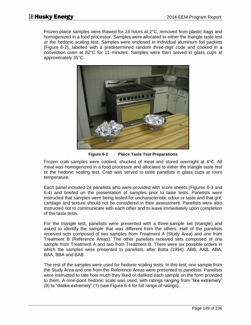
Submitted To 2014 EEM Program Report
Page 149 of 236
Frozen plaice samples were thawed for 24 hours at 2°C, removed from plastic bags and homogenized in a food processor. Samples were allocated to either the triangle taste test or the hedonic scaling test. Samples were enclosed in individual aluminum foil packets (Figure 6-2), labelled with a predetermined random three-digit code and cooked in a convection oven at 82°C for 11 minutes. Samples were then served in glass cups at approximately 35°C.
Figure 6-2 Plaice Taste Test Preparations
Frozen crab samples were cooked, shucked of meat and stored overnight at 4°C. All meat was homogenized in a food processor and allocated to either the triangle taste test or the hedonic scaling test. Crab was served to taste panelists in glass cups at room temperature.
Each panel included 24 panelists who were provided with score sheets (Figures 6-3 and 6-4) and briefed on the presentation of samples prior to taste tests. Panelists were instructed that samples were being tested for uncharacteristic odour or taste and that grit, cartilage and texture should not be considered in their assessment. Panelists were also instructed not to communicate with each other and to leave immediately upon completion of the taste tests.
For the triangle test, panelists were presented with a three-sample set (triangle) and asked to identify the sample that was different from the others. Half of the panelists received sets composed of two samples from Treatment A (Study Area) and one from Treatment B (Reference Areas). The other panelists received sets composed of one sample from Treatment A and two from Treatment B. There were six possible orders in which the samples were presented to panelists, after Botta (1994): ABB, AAB, ABA, BAA, BBA and BAB.
The rest of the samples were used for hedonic scaling tests. In this test, one sample from the Study Area and one from the Reference Areas were presented to panelists. Panelists were instructed to rate how much they liked or disliked each sample on the form provided to them. A nine-point hedonic scale was used, with ratings ranging from “like extremely” (9) to “dislike extremely” (1) (see Figure 6-4 for full range of ratings).

Submitted To 2014 EEM Program Report
Page 150 of 236
QUESTIONNAIRE FOR TRIANGLE TEST
Name: Date/Time: Product: American Plaice
1. Taste the samples in the order indicated and identify the odd sample. You must choose one of the samples.
Code Check Odd Sample
214
594
733
2. Comments: ________________________________________________________________ ________________________________________________________________ ________________________________________________________________ ________________________________________________________________ ________________________________________________________________ ________________________________________________________________ ________________________________________________________________ ________________________________________________________________
Figure 6-3 Questionnaire for Taste Evaluation by Triangle Test

Submitted To 2014 EEM Program Report
Page 151 of 236
QUESTIONNAIRE FOR HEDONIC SCALING
Name: Date/Time:
Product: American Plaice
1. Taste these samples and check how much you like or dislike each one.
619 835
like extremely like extremely
like very much like very much
like moderately like moderately
like slightly like slightly
neither like nor neither like nor
dislike dislike
dislike slightly dislike slightly
dislike moderately dislike moderately
dislike very much dislike very much
dislike extremely dislike extremely
2. Comments:
Figure 6-4 Questionnaire for Taste Evaluation by Hedonic Scaling
6.1.2.4 Fish Health Indicators
Blood smears were stained with Giemsa stain and examined with a Wild Leitz Aristoplan bright field microscope to identify different types of cells based on their general form and affinity to the dye after methods in Ellis (1976).
MFO induction was assessed in liver samples of plaice as 7-ethoxyresorufin O-deethylase (EROD) activity according to the method of Pohl and Fouts (1980) as modified by Porter et al. (1989).
Fixed liver and gill samples were processed by standard histological methods (Lynch et al. 1969).
Details on these methods are provided in Appendix C-3.

Submitted To 2014 EEM Program Report
Page 152 of 236
6.1.3 Data Analysis
6.1.3.1 Overview
For most analyses except taste tests, the commercial fish component of the White Rose EEM program uses a multiple-reference design, with four Reference Areas and a single Study Area. Such designs are common in environmental monitoring programs when a single Study Area of interest (i.e., one production area) exists (Underwood 1993). The goal of these “asymmetrical” designs is to assess for potential environmental effects at a Study Area relative to the average of many representative Reference Areas. Using multiple Reference Areas better estimates the natural variability in environmental conditions of the larger region, thus providing a more accurate benchmark against which to compare environmental conditions at the Study Area.
Taste test results from the triangle and hedonic scaling test compared Study Area samples to pooled Reference Area samples, as methods for these tests using multiple reference Areas are unavailable.
6.1.3.2 Biological Characteristics
Biological characteristics (morphometric and life history characteristics) of plaice and crab were analyzed to determine if there were differences among composites that could affect results of body burden analyses. Analyses were restricted to plaice and crab used for body burden analyses in 2014. Formal comparisons among years were not conducted.
Plaice
Composite mean gutted weights of plaice were compared among Areas in ANOVA to test for differences in size among Reference Areas and between Reference and Study Areas for chemistry composites. Additional analyses on plaice biological characteristics and condition were performed to support Fish Health Analyses. Differences in maturity stages between the Study and Reference Areas were assessed with Fisher's Exact Test. Biological characteristics and condition were compared among Areas via ANOVA (or ANCOVA equivalents for condition or liver and gonad indices). Total length, gutted weight and age were analyzed using ANOVA (i.e., with no covariate or X variable). The regression analogues of three condition indices - Fulton Condition Factor (CF), Hepatosomatic Index (HSI) and Gonadosomatic Index (GSI) - were analyzed via ANCOVA, which compares regression intercepts or adjusted means among Areas. Differences among Reference Areas and between the Reference and Study Areas were tested.
Crab
Biological characteristics of crab included carapace width and claw height (i.e., size), and frequency of recent moults based on the shell condition index. Recent moults included crab with shell condition index values of 1 or 2. Non-recent moults included crab with condition index values of 6 (probably one year since moult) and 3 or 4 (two or more years since moult).
Asymmetrical ANOVA was used to test for significant differences in carapace width and claw height between the Reference and Study Areas.

Submitted To 2014 EEM Program Report
Page 153 of 236
6.1.3.3 Body Burden
Plaice
Spatial Variations in 2014
Body burden data from composite samples were available for both liver and fillet tissue. Variables associated with liver tissue that were statistically analyzed were those that were frequently detected14 and included fat content, moisture content, concentrations of eight metals frequently detected (arsenic, cadmium, copper, iron, manganese, selenium, strontium and zinc) and >C10-C21 and >C21-C32 hydrocarbon concentrations. Values less than laboratory detection limits were set at ½ laboratory detection limits.
Fewer variables were detected in plaice fillets. Variables analyzed in fillets were fat content, moisture content and concentrations of arsenic, iron, mercury, strontium and zinc.
Log-transformed values for liver and fillets were compared among Areas in an asymmetrical one-way ANOVA.
Variations in Temporal Trends
Differences in temporal trends in plaice liver variables were tested using a two-way asymmetrical ANOVA of composite tissue concentrations from 2004, 2005, 2006, 2010, 2012 and 2014 (Table 6-5). In this ANOVA, linear orthogonal contrasts (Hoke et al. 1990) were used to test for differences in linear and quadratic time trends between Reference and Study Areas. Variations were judged relative to variations in average concentrations among Reference Areas (i.e., the Among-Reference Term in Table 6-5).
Table 6-5 Completely Random ANOVA Used for Comparison of Body Burden Variables Among Years (2004, 2005, 2006, 2010, 2012 and 2014)
Source/Term df Description
Study vs Reference (SR) 1 Tests for differences in concentration between Study and Reference Areas that are consistent across years
Year (overall) 5 Tests for differences in concentration among years that are consistent in both Study and Reference Areas
Linear Trend 1 Tests for a linear trend that is similar across all areas
Quadratic Trend 1 Tests for a trend that involves an increase followed by a decrease (or vice versa), in a fashion that is similar across all areas
SR x Year 5 Tests for variations in concentration between Study and Reference Areas that change from year to year
SR x Linear Trend 1 Tests for differences in linear time trends between the Reference and Study Areas
SR x Quadratic Trend 1 Tests for differences in quadratic time trends between the Reference and Study Areas
Among References (= Error) 15 Natural variance in concentrations among Reference Areas within years
14 Variables with greater than 25% of test results below laboratory detection limits were not included in
statistical analyses.

Submitted To 2014 EEM Program Report
Page 154 of 236
Data from 2000 were not included in analyses because Reference Area data were collected in different locations during that year (see Husky Energy 2004 for details on baseline collections). Data from 2008 were also excluded because data were not collected from Reference Areas 3 and 4 because of intense fishing activity in those two Reference Areas at the time of the survey. However, the data from the Study Area and Reference Areas in 2008 were included in scatter plots, so it was possible to visually inspect those data and compare them to data before and after that year.
Crab
Spatial Variations in 2014
Crab leg body burden variables analyzed were fat and moisture content as well as concentrations of eight frequently detected metals (arsenic, copper, iron, mercury, selenium, silver, strontium and zinc). Values less than laboratory detection limits were set at ½ laboratory detection limits. Variables with greater than 25% of test results below laboratory detection limits were not included in statistical analyses.
Log-transformed values for the above variables, except percent fat which was rank transformed, were compared among Areas with an asymmetrical one-way ANOVA.
Variations in Temporal Trends
Differences in temporal trends in crab tissue variables were tested using a two-way asymmetrical ANOVA of composite tissue concentrations from 2004, 2005, 2006, 2010, 2012 and 2014 (Table 6-5), as described above. As for plaice liver and fillets, linear orthogonal contrasts (Hoke et al. 1990) were used to test for differences in linear and quadratic time trends between Reference and Study Areas. Variations were judged relative to variations in average concentrations among Reference Areas (i.e., the Among-Reference Term in Table 6-5).
As with plaice, data from baseline were not included in these analyses because Reference Area data were collected in different locations. Data from 2008 were excluded because data were not collected from Reference Areas 3 and 4 because of intense fishing activity in those two Reference Areas at the time of the survey. However, the data from the Study Area and Reference Areas in 2008 were included in scatter plots, so it was possible to visually inspect those data and compare them to data before and after that year.
6.1.3.4 Taste Tests
As noted above, triangle tests and hedonic scaling tests compared Study Area samples to pooled Reference Area samples.
The triangle test datum is the number of correct sample identifications over the number of panelists. This value was calculated and compared to values in Appendix C-4 (after Larmond 1977) to determine statistical significance. For a panel size of 24, a statistically
significant discrimination between Areas (at = 0.05) requires that 13 panelists correctly identify samples.
Hedonic scaling results were processed in ANOVA and presented graphically in frequency histograms.

Submitted To 2014 EEM Program Report
Page 155 of 236
Ancillary comments from panelists were tabulated and qualitatively assessed for both tests.
6.1.3.5 Fish Health Indicators
Biological Characteristics
Sex Ratio and Maturity Stages
The Fisher’s Exact Test was used to compare maturity stages between the Study Area and the combined Reference Areas (SR contrast) for female fish. Statistical analyses of maturity stages for male fish or sex ratios (male to female) between the Study Area and Reference Areas were not conducted because of low sample size for male fish.
Size, Age and Condition
Variables for each sex were compared among Areas via ANOVA (or ANCOVA equivalents for condition or liver and gonad indices; see below). Both the Among-Reference and Study versus Reference contrasts were tested.
Total length, gutted weight and age were analyzed using ANOVA (i.e., with no covariate or X variable).
The regression analogues of three condition indices (Fulton Condition Factor, Hepatosomatic Index and Gonadosomatic Index) were analyzed via ANCOVA which compares regression intercepts or adjusted means among Areas.
Mixed Function Oxygenase Activity
ANOVAs were used to compare MFO activity in pre-spawning and spent females. MFO values were log-transformed for analyses.
Histopathology
Both male and female fish from each Area were combined for histopathological analysis.
Liver Histopathology
The Fisher’s Exact Test was used to compare presence versus absence of biliary parasites between the Study Area versus the Reference Areas. Other liver abnormalities were rare or absent and were not statistically analyzed.
Gill Histopathology
The Fisher’s Exact Test was used to compare frequencies of fish with at least one lamella affected by the different lesions between the Study Area and Reference Areas.
6.2 Results
6.2.1 Biological Characteristics
6.2.1.1 Plaice
Summary statistics for composite mean gutted weights of plaice are provided in Table 6-6.

Submitted To 2014 EEM Program Report
Page 156 of 236
Table 6-6 Summary Statistics for Plaice Composite Mean Gutted Weight (g) (2014)
Area n Min Max Mean SD
Reference 1 3 538 1140 833 163
Reference 2 3 518 1174 756 152
Reference 3 3 536 1768 1012 304
Reference 4 3 710 2350 1142 292
Reference Average 12 576 1608 936 228
Study 10 502 1570 910 223
Note: - n = number of composites per Area. Refer to Table 6-2 for number of fish per composite.
Variations in mean fish weight within composites differed significantly among Reference Areas (p = 0.012) but did not vary significantly between the Study and Reference Areas (p = 0.998, Table 6-7). The average Reference Area fish was 936 g ± 228 g, while the average Study Area fish was 910 g ± 223 g. The box plot in Figure 6-5 illustrates the spread of gutted weights among the Reference Areas, and shows that the range of gutted weights in Reference Area fish was greater than the range of gutted weights in Study Area fish.
Table 6-7 Results of ANOVA Comparing Plaice Composite Mean Gutted Weight (g) Among Areas (2014)
Source SS df MS F-Ratio p-value
Reference vs Study 0.13 1 0.13 0.00001 0.998
Among Reference 272,995 3 90,998 7.198a 0.012
Error 277,141 17 16,302
Note: - a F-ratio calculated using MS error from separate one-way ANOVA testing for differences among Reference Areas 1 to 4 (MS = 12,643; df = 8).
Ref 1 Ref 2 Ref 3 Ref 4 Study
Area
600
700
800
900
1,000
1,100
1,200
1,300
Gu
tted
Weig
ht
(g)
Figure 6-5 Box Plot of Plaice Gutted Weight (g)
Notes: The centre line is the median. Ends of the box indicate the lower and upper quartiles. Ends of the whiskers indicate the quartile ±1.5 x interquartile spread. Asterisks, where they are present, would indicate values falling within the quartile ±3 x interquartile spread. Open circles would indicate values falling outside
the quartile ±3 x interquartile spread.

Submitted To 2014 EEM Program Report
Page 157 of 236
Additional analyses on biological characteristics and condition of plaice by sex and maturity stage is undertaken within the context of fish health indicator assessment (Appendix C-3). More relevant information is provided below, with details in Appendix C-3.
Female plaice greatly outnumbered males in all Areas (Table 6-8), and there were too few males collected to undertake statistical analyses of biological characteristics and condition.
Table 6-8 Numbers of Female and Male Plaice (2014)
Area Females Males Total
Number % Number % Number
Reference Area 1 30 100 0 0 30
Reference Area 2 30 100 0 0 30
Reference Area 3 30 100 0 0 30
Reference Area4 29 96.7 1 3.33 30
All Reference Areas 119 99.2 1 0.833 120
Study Areas 100 100 0 0 100
All Areas 219 99.5 1 0.455 220
Virtually all females examined (98%) were mature (n = 217 of 219 fish), and 10% were spent (n = 22 of 219 fish) (Table 6-9). Frequencies of pre-spawning and spent mature females varied significantly between the combined Reference Areas and the Study Area (Fisher’s Exact test, p = 0.025).
Table 6-9 Frequency of Maturity Stages of Female Plaice (2014)
Area
Immature F-500 a
Maturing to spawn this year F-510 to F-540 a
Partly spent F-550 a
Spent this year F-560+F-570 a
Total
Number % Number % Number % Number % Number
Reference Area 1
0 0 29 97 0 0 1 3 30
Reference Area 2
1 3 23 77 0 0 6 20 30
Reference Area 3
0 0 22 73 0 0 8 27 30
Reference Area 4
1 3 26 90 0 0 2 7 29
All References
2 2 100 84 0 0 17 14 119
Study Area 2 2 93 93 1 1 4 4 100
All Areas
4 2 193 88 1 0 21 10 219
Note: - a Maturity stages were defined according to procedures used by DFO (Appendix C-3, Annex A)
Since female fish undergo physical and physiological changes during their reproductive period, it can be informative to carry out comparisons of biological characteristics and condition between like maturity stages, when numbers permit. In 2014, sufficient numbers of pre-spawning females (stages F-510 to F-540) and spent females (stage F560 to F580) were caught to allow comparison.
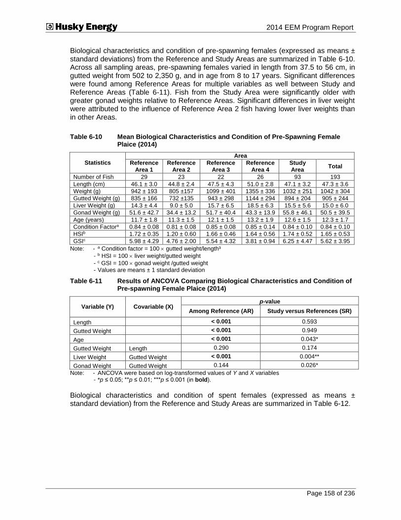
Submitted To 2014 EEM Program Report
Page 158 of 236
Biological characteristics and condition of pre-spawning females (expressed as means ± standard deviations) from the Reference and Study Areas are summarized in Table 6-10. Across all sampling areas, pre-spawning females varied in length from 37.5 to 56 cm, in gutted weight from 502 to 2,350 g, and in age from 8 to 17 years. Significant differences were found among Reference Areas for multiple variables as well between Study and Reference Areas (Table 6-11). Fish from the Study Area were significantly older with greater gonad weights relative to Reference Areas. Significant differences in liver weight were attributed to the influence of Reference Area 2 fish having lower liver weights than in other Areas.
Table 6-10 Mean Biological Characteristics and Condition of Pre-Spawning Female Plaice (2014)
Statistics
Area
Reference Area 1
Reference Area 2
Reference Area 3
Reference Area 4
Study Area
Total
Number of Fish 29 23 22 26 93 193
Length (cm) 46.1 ± 3.0 44.8 ± 2.4 47.5 ± 4.3 51.0 ± 2.8 47.1 ± 3.2 47.3 ± 3.6
Weight (g) 942 ± 193 805 ±157 1099 ± 401 1355 ± 336 1032 ± 251 1042 ± 304
Gutted Weight (g) 835 ± 166 732 ±135 943 ± 298 1144 ± 294 894 ± 204 905 ± 244
Liver Weight (g) 14.3 ± 4.4 9.0 ± 5.0 15.7 ± 6.5 18.5 ± 6.3 15.5 ± 5.6 15.0 ± 6.0
Gonad Weight (g) 51.6 ± 42.7 34.4 ± 13.2 51.7 ± 40.4 43.3 ± 13.9 55.8 ± 46.1 50.5 ± 39.5
Age (years) 11.7 ± 1.8 11.3 ± 1.5 12.1 ± 1.5 13.2 ± 1.9 12.6 ± 1.5 12.3 ± 1.7
Condition Factora 0.84 ± 0.08 0.81 ± 0.08 0.85 ± 0.08 0.85 ± 0.14 0.84 ± 0.10 0.84 ± 0.10
HSIb 1.72 ± 0.35 1.20 ± 0.60 1.66 ± 0.46 1.64 ± 0.56 1.74 ± 0.52 1.65 ± 0.53
GSIc 5.98 ± 4.29 4.76 ± 2.00 5.54 ± 4.32 3.81 ± 0.94 6.25 ± 4.47 5.62 ± 3.95
Note: - a Condition factor = 100 gutted weight/length³
- b HSI = 100 liver weight/gutted weight
- c GSI = 100 gonad weight /gutted weight - Values are means ± 1 standard deviation
Table 6-11 Results of ANCOVA Comparing Biological Characteristics and Condition of Pre-spawning Female Plaice (2014)
Variable (Y) Covariable (X) p-value
Among Reference (AR) Study versus References (SR)
Length < 0.001 0.593
Gutted Weight < 0.001 0.949
Age < 0.001 0.043*
Gutted Weight Length 0.290 0.174
Liver Weight Gutted Weight < 0.001 0.004**
Gonad Weight Gutted Weight 0.144 0.026*
Note: - ANCOVA were based on log-transformed values of Y and X variables - *p ≤ 0.05; **p ≤ 0.01; ***p ≤ 0.001 (in bold).
Biological characteristics and condition of spent females (expressed as means ± standard deviation) from the Reference and Study Areas are summarized in Table 6-12.

Submitted To 2014 EEM Program Report
Page 159 of 236
Table 6-12 Biological Characteristics and Condition of Spent Female Plaice (2014)
Statistics
Area
Reference Area 1
Reference Area 2
Reference Area 3
Reference Area 4
Study Area Total
Number of Fish
1 6 8 2 4 21
Length (cm) 45.8 47.8 ± 6.3 53.7 ± 5.1 50.5 ± 1.3 49.4 ± 3.7 50.5 ± 5.4
Weight (g) 832.0 936 ± 223 1478 ± 452 1188 ± 51 1142 ± 342 1201 ± 401
Gutted Weight (g)
776.0 847 ± 205 1201 ± 245 1017 ± 83 1014 ± 308 1026 ± 266
Liver Weight (g)
12.0 12.0 ± 4.0 17.5 ± 5.1 17.0 ± 1.4 13.0 ± 5.3 14.8 ± 4.9
Gonad Weight (g)
30.0 32.3 ± 11.3 60.6 ± 23.5 49.0 ± 4.2 68.5 ± 41.4 51.5 ± 26.6
Age (years) 11.0 12.0 ± 2.1 13.1 ± 1.0 12.5 ± 2.1 13.3 ± 1.0 12.7 ± 1.5
Condition Factora
0.81 0.78 ± 0.12 0.79 ± 0.15 0.79 ± 0.00 0.82 ± 0.11 0.79 ± 0.12
HSIb 1.55 1.43 ± 0.40 1.46 ± 0.33 1.67 ± 0.00 1.26 ± 0.16 1.44 ± 0.30
GSIc 3.87 3.76 ± 0.70 5.00 ± 1.26 4.82 ± 0.02 6.51 ± 2.15 4.86 ± 1.53
Note: - a Condition factor = 100 gutted weight/length³
- b HSI = 100 liver weight/gutted weight
- c GSI = 100 gonad weight /gutted weight - Values are means ± 1 standard deviation
Across all sampling locations, spent females varied in length from 42.5 to 60.1 cm, in gutted weight from 622 to 1,528 g, and in age from 10 to 15 years. There was only one spent female collected from Reference Area 1. Significant differences were found among Reference Areas for gutted weight, as well as between the Study and Reference Areas for gonad weight relative to gutted weight (Table 6-13). Fish from the Study Area had greater gonad weights relative to gutted weight than did fish from the Reference Areas.
Table 6-13 Results of ANCOVA Comparing Biological Characteristics and Condition of Spent Females Plaice (2014)
Variable (Y) Covariable (X) p-value
Among Reference (AR) Study versus References (SR)
Length 0.135 0.557
Gutted Weight 0.046* 0.914
Age 0.401 0.468
Gutted Weight Length 0.028 0.143
Liver Weight Gutted Weight 0.614 0.326
Gonad Weight Gutted Weight 0.423 0.008**
Note: - ANCOVA were based on log-transformed values of Y and X variables - *p ≤ 0.05; **p ≤ 0.01; ***p ≤ 0.001 (in bold).
6.2.1.2 Crab
Shell condition index values for the crab collected in 2014 and used for body burden analyses are provided in Table 6-14. All (100%) of the crab collected had moulted in 2013 (Table 6-14).

Submitted To 2014 EEM Program Report
Page 160 of 236
Table 6-14 Number (and %) of Crab and Associated Index Values (2014)
Index Value Year of Molt Area
Ref 1 Ref 2 Ref 3 Ref 4 All Ref Study
1,2 2014 0% 0% 0% 0% 0% 0%
6 2013 100% 100% 100% 100% 100% 100%
3,4 2012 or earlier 0% 0% 0% 0% 0% 0%
Total Crabs (n) 18 35 34 18 105 82
Summary statistics for composite means for carapace width and claw height are provided in Table 6-15. Crab carapace width and claw height differed significantly between the Reference and Study Areas (Table 6-16), with mean carapace widths of 115 and 108 mm for Reference and Study Areas, respectively (Table 6-15). Similar differences were observed with mean claw heights of 27.8 and 25.0 mm for Reference and Study Areas, respectively (Table 6-15). Crab size also varied significantly among the Reference Areas (Table 6-16). In general, crab from Reference Area 3 and the Study Area were similar in size; crab from the remaining Reference Areas were slightly larger (Table 6-15).
Table 6-15 Summary Statistics for Biological Characteristics of Crab Based on Composite Mean Carapace Width and Claw Height (2014)
Variable Area n Min Max Mean SD
Carapace width (mm)
Reference Area 1 3 108 137 118 7.09
Reference Area 2 3 99 133 114 6.93
Reference Area 3 3 76 122 107 10.6
Reference Area 4 3 108 140 123 9.22
Reference mean 12 97.8 133 115 8.46
Study Area 10 79.0 136 108 10.1
Claw height (mm)
Reference Area 1 3 23.0 44.0 29.3 4.41
Reference Area 2 3 17.0 35.0 26.0 3.44
Reference Area 3 3 14.0 32.0 24.7 3.85
Reference Area 4 3 25.0 41.0 31.1 3.89
Reference mean 12 19.8 38.0 27.8 3.90
Study Area 10 11.0 36.0 25.0 4.26
Table 6-16 Results of ANOVA Comparing Crab Biological Characteristics Among Areas (2014)
Variable Source Type III SS df Mean Squares F-Ratio p-value
Carapace Width
Study vs Reference 268.34 1.00 268.34 15.07 0.001
Among Reference 318.43 3.00 106.14 5.17a 0.010*
Error 302.74 17.00 17.81
Claw Height
Study vs Reference 54.30 1.00 54.30 13.30 0.002**
Among Reference 59.82 3.00 19.94 4.48b 0.017*
Error 69.40 17.00 4.08
Notes: - *p ≤ 0.05; **p ≤ 0.01; ***p ≤ 0.001 (in bold).
- a F-ratio calculated using MS error from separate one-way ANOVA testing for differences among Reference Area 1 to 4 (MS = 20.527; df = 8).
- b F-ratio calculated using MS error from separate one-way ANOVA testing for differences among Reference Area 1 to 4 (MS = 4.446; df = 8).

Submitted To 2014 EEM Program Report
Page 161 of 236
6.2.2 Body Burden
6.2.2.1 Plaice
Liver
Summary statistics for detected substances in plaice liver in 2004, 2005, 2006, 2008, 2010, 2012 and 2014 and raw data for 2014 are provided in Appendix C-2. Arsenic, cadmium, copper, iron, manganese, mercury, selenium and zinc were detected frequently in all years. These eight metals, fat and moisture content and >C10-C21 and >C21-C32 hydrocarbon concentrations are analyzed quantitatively. Hydrocarbons in the >C10-C21 and >C21-C32 range detected in all years have shown no resemblance to drill fluid or petroleum hydrocarbons (J. Kiceniuk, pers. comm.; Maxxam Analytics, pers. comm.; petroforma inc., pers. comm.), and similar compounds also have been consistently observed in liver tissue at the nearby Terra Nova site (Suncor Energy 2013). As in previous years, additional Gas Chromatography/Mass Spectrometer analysis of two liver samples in 2014 indicated that there was no indication of drill fluid or petroleum hydrocarbons in those samples.
In 2014, low levels of acenaphthene were detected in one liver sample from Reference Area 3. Low levels of naphthalene were detected in one sample from Reference Area 1 and one sample from Reference Area 3. Low levels of phenanthrene were detected in one sample from the Study Area. Low levels of naphthalene were detected in one sample from Reference Area 2 in 2012 (Appendix C-2).
Spatial Variations in 2014
The results of ANOVA are presented in Table 6-17, and the spatial variations in variable concentrations are illustrated in the box plots in Figure 6-6. Cadmium and selenium concentrations varied significantly among Reference Areas (p ≤ 0.001; Table 6-11). Percent fat, percent moisture and concentrations of cadmium, zinc and >C21-C32
hydrocarbons all varied significantly between the Reference Areas and Study area (Table 6-17). Percent fat and the concentration of >C21-C32 hydrocarbons were generally lower in the Study Area. Percent moisture and concentrations of cadmium and zinc were generally higher in the Study Area (Figure 6-6).
Table 6-17 Results of ANOVA Comparing Plaice Liver Body Burden Variables among Areas (2014)
Variable p-values
Among Reference Reference vs Study
Fat 0.264 0.027*
Moisture 0.119 0.012*
Arsenic 0.717 0.381
Cadmium ≤ 0.001*** 0.015*
Copper 0.824 0.091
Iron 0.124 1.000
Manganese 0.500 1.000
Selenium ≤ 0.001*** 1.000
Strontium 0.191 0.214
Zinc 0.028* 0.005**
>C10-C21 0.196 0.171
>C21-C32 0.126 0.012*
Notes: - Values are probabilities of no difference among areas, or no difference among or between the Areas.
- Variables were log10 transformed prior to analysis. - *p ≤ 0.05; **p ≤ 0.01; ***p ≤ 0.001 (in bold).
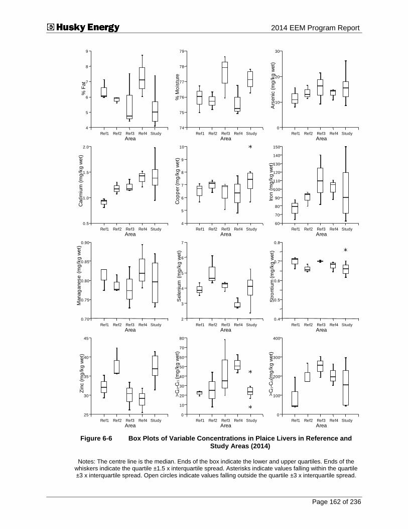
Submitted To 2014 EEM Program Report
Page 162 of 236
Ref1 Ref2 Ref3 Ref4 Study
Area
4
5
6
7
8
9
% F
at
Ref1 Ref2 Ref3 Ref4 Study
Area
74
75
76
77
78
79
% M
ois
ture
Ref1 Ref2 Ref3 Ref4 Study
Area
0
10
20
30
Ars
enic
(m
g/k
g w
et)
Ref1 Ref2 Ref3 Ref4 Study
Area
0.5
1.0
1.5
2.0
Cad
miu
m (
mg
/kg
wet)
Ref1 Ref2 Ref3 Ref4 Study
Area
4
5
6
7
8
9
10
Co
pp
er (m
g/k
g w
et)
Ref1 Ref2 Ref3 Ref4 Study
Area
60
70
80
90
100
110
120
130
140
150
Iro
n (
mg
/kg
wet)
Ref1 Ref2 Ref3 Ref4 Study
Area
0.70
0.75
0.80
0.85
0.90
Manag
anese (
mg
/kg
wet)
Ref1 Ref2 Ref3 Ref4 Study
Area
2
3
4
5
6
7
Sele
niu
m (
mg
/kg
wet)
Ref1 Ref2 Ref3 Ref4 Study
Area
0.4
0.5
0.6
0.7
0.8
Str
ontium
(m
g/k
g w
et)
Ref1 Ref2 Ref3 Ref4 Study
Area
25
30
35
40
45
Zin
c (m
g/k
g w
et)
Ref1 Ref2 Ref3 Ref4 Study
Area
0
10
20
30
40
50
60
70
80
>C
10-C
21(m
g/k
g w
et)
Ref1 Ref2 Ref3 Ref4 Study
Area
0
100
200
300
400
>C
21-C
32(m
g/k
g w
et)
Figure 6-6 Box Plots of Variable Concentrations in Plaice Livers in Reference and Study Areas (2014)
Notes: The centre line is the median. Ends of the box indicate the lower and upper quartiles. Ends of the whiskers indicate the quartile ±1.5 x interquartile spread. Asterisks indicate values falling within the quartile ±3 x interquartile spread. Open circles indicate values falling outside the quartile ±3 x interquartile spread.

Submitted To 2014 EEM Program Report
Page 163 of 236
Variations in Temporal Trends
Variations in mean concentrations of frequently detected variables in plaice livers between 2004 and 201415 are illustrated in Figure 6-7. Significant area-wide trends were noted for all variables (Table 6-18). Manganese and >C10-C21 hydrocarbon concentrations decreased over time, in all areas. Zinc concentrations increased over time, in all areas. Percent fat, percent moisture, arsenic, cadmium, copper, iron and selenium produced a strong quadratic effect (p < 0.001), which means that concentrations increased and then decreased, or vice versa. This occurred in all Areas (Figure 6-7). >C21-C32 hydrocarbons produced a weaker quadratic effect across all Areas (p = 0.032). A weakly statistically significant linear difference between the Reference Areas and the Study Area was observed for percent moisture (p = 0.041, Table 6-18). Averaged across all years, percent moisture concentrations in the Study Area were higher by a mean of 0.2% compared to the Reference Areas (although this difference is not apparent from Figure 6-7). There was also a significant difference (p = 0.002) in changes in concentrations of >C21-C32 hydrocarbons, likely influenced by lower concentrations in the Reference Areas in 2006 and 2010 (Figure 6-7).
Table 6-18 Results of ANOVA Testing for Differences in Average Plaice Liver Body Burden Variables and Temporal Trends Between the Reference and Study Areas (2004 to 2014)
Variable
Linear Quadratic
Area-Wide Trend
Difference Between Reference and Study
Area-Wide Trend
Difference Between Reference and Study
Fat <0.001*** 0.202 <0.001*** 0.309
Moisture <0.001*** 0.041* <0.001*** 1.000
Arsenic <0.001*** 0.076 <0.001*** 0.502
Cadmium <0.001*** 0.826 <0.001*** 0.756
Copper <0.001*** 0.700 <0.001*** 0.700
Iron <0.001*** 0.559 0.001*** 1.000
Manganese 0.013* 0.711 0.302 1.000
Selenium <0.001*** 0.333 <0.001*** 0.624
Zinc <0.001*** 1.000 0.216 0.333
>C10-C21 <0.001*** 0.765 1.000 0.086
>C21-C32 <0.001*** 0.126 0.032* 0.002**
Notes: - Values are probabilities of no temporal trend or no difference in temporal trends. - Variables were log10 transformed prior to analysis. - 2008 data were excluded from ANOVA because all Reference Areas were not sampled in that
year. - *p ≤ 0.05; **p ≤ 0.01; ***p ≤ 0.001 (in bold).
15 Data from 2000 were not included in ANOVA analyses because Reference Area data were collected in
different locations during that year. Data from 2008 were also excluded from the ANOVA analyses because data were not collected from Reference Areas 3 and 4 because of intense fishing activity in those two Reference Areas at the time of the survey. Data from 2008 are included in scatter plots.

Submitted To 2014 EEM Program Report
Page 164 of 236
Year
5
10
15
20
Perc
ent
Fat
Year
64
68
72
76
Perc
ent
Mo
istu
re
Year
0
10
20
30
40
Ars
enic
(m
g/k
g w
et)
Year
0.2
0.4
0.6
0.8
1.0
1.2
1.4
Cad
miu
m (
mg
/kg
wet)
Year
3
4
5
6
7
8
9
10
Co
pp
er (m
g/k
g w
et)
Year
40
60
80
100
120
Iro
n (
mg
/kg
wet)
Year
0.6
0.7
0.8
0.9
1.0
1.1
1.2
Mang
anese (
mg
/kg
wet)
Year
0.01
0.02
0.03
0.04
0.05
0.06
0.07
Merc
ury
(m
g/k
g w
et)
Year
1.5
2.0
2.5
3.0
3.5
4.0
4.5
5.0
Sele
niu
m (
mg
/kg
wet)
Year
24
28
32
36
40
Zin
c (m
g/k
g w
et)
Year
20
40
60
80
100
120
140
>C
10-C
21(m
g/k
g w
et)
Year
50
100
150
200
250
>C
21-C
32(m
g/k
g w
et)
Study
Reference
Figure 6-7 Variations in Area Means of Detectable Metals and Hydrocarbons in Plaice Liver Composites from 2004 and 2014
Note: Values shown are annual averages within Areas. Red circles are Study Area averages; open circles are averages for each Reference Area.

Submitted To 2014 EEM Program Report
Page 165 of 236
Fillets
Summary statistics for concentrations of detected substances in 2004, 2005, 2006, 2008, 2010, 2012 and 2014, and raw data for 2014 are provided in Appendix C-2. Arsenic, mercury and zinc were detected frequently in plaice fillet tissue in all years. Iron and strontium were detected frequently in 2014, but these metals were detected only sporadically in previous years. 2014 data for these metals and fat and moisture content were analyzed quantitatively. Multi-year comparisons included arsenic, mercury, zinc and fat and moisture content.
Boron, copper, lead, nickel and selenium were detected sporadically in fillets in some years (Appendix C-2). One fillet sample from Reference Area 4 had detectable compounds in the >C10-C21 hydrocarbon range in 2005, two samples from the same Area had detectable compounds in the >C10-C21 and >C21-C32 hydrocarbon ranges in 2006, and one sample from Reference Area 3 had detected levels of compounds in the >C10-C32 hydrocarbon range in 2014. However, chromatograms for these samples did not indicate the presence of drill muds or petrogenic compounds (J. Kiceniuk, pers. comm.; petroforma inc., pers. comm.). In 2014, low levels of acenaphthene were detected in seven fillet samples from Reference Areas, and one fillet sample from the Study Area (Appendix C-2). Low levels of naphthalene were detected in one fillet sample from the Study Area (Appendix C-2).
Spatial Variations in 2014
ANOVA was used to test for differences between the Reference Areas and the Study Area in fat, moisture and metals (arsenic, iron, mercury, strontium and zinc) concentrations of plaice fillets, and data are plotted in Figure 6-8. There were no differences in concentrations between the Reference Areas and the Study Area. A difference in concentration among Reference Areas was noted for strontium (Table 6-19). Strontium concentrations were higher in Reference Area 3 (Figure 6-8).
Table 6-19 Results of ANOVA Comparing Plaice Fillet Body Burden Variables among Areas (2014)
Variable p-values
Among Reference Study vs Reference
Fat 0.381 0.623
Moisture 0.381 0.691
Arsenic 0.112 1.000
Iron 0.052 0.414
Mercury 0.556 0.818
Strontium 0.002** 0.643
Zinc 0.077 0.109
Notes: - Values are probabilities of no difference among Areas, or between Reference and Study Areas. - Variables were log10 transformed prior to analysis. - *p ≤ 0.05; **p ≤ 0.01; ***p ≤ 0.001 (in bold).

Submitted To 2014 EEM Program Report
Page 166 of 236
Ref1 Ref2 Ref3 Ref4 Study
Area
0.5
0.6
0.7
0.8
0.9
1.0
1.1
1.2
1.3
Perc
ent F
at
Ref1 Ref2 Ref3 Ref4 Study
Area
82
83
84
85
86
Perc
ent M
ois
ture
Ref1 Ref2 Ref3 Ref4 Study
Area
3
4
5
6
7
8
Ars
enic
(m
g/k
g w
et)
Ref1 Ref2 Ref3 Ref4 Study
Area
0
1
2
3
4
5
Iron (
mg/k
g w
et)
Ref1 Ref2 Ref3 Ref4 Study
Area
0.00
0.05
0.10
0.15
0.20
Merc
ury
(m
g/k
g w
et)
Ref1 Ref2 Ref3 Ref4 Study
Area
0.2
0.3
0.4
0.5
0.6
0.7
0.8
0.9
1.0
Str
ontiu
m (
mg/k
g w
et)
Ref1 Ref2 Ref3 Ref4 Study
Area
2
3
4
5
6
7
8
9
10
11
Zin
c (m
g/k
g w
et)
Figure 6-8 Box Plots of Variable Concentrations in Plaice Fillets in Reference and
Study Areas (2014)
Notes: The centre line is the median. Ends of the box indicate the lower and upper quartiles. Ends of the whiskers indicate the quartile ±1.5 x interquartile spread. Asterisks indicate values falling within the quartile ±3 x interquartile spread. Open circles indicate values falling outside the quartile ±3 x interquartile spread.

Submitted To 2014 EEM Program Report
Page 167 of 236
Variations in Temporal Trends
Significant area-wide trends were seen for fillet fat and moisture content and arsenic, mercury and zinc concentrations. Percent fat decreased over time and percent moisture generally increased over time in both the Study and Reference Areas. Significant area-wide quadratic trends (in this case, a decrease followed by an increase) were seen for arsenic, mercury and zinc (Table 6-20; Figure 6-9). Zinc concentrations demonstrated significant differences in linear time trends between the Reference and Study Areas (p = 0.002). Further examination of the data indicated that this difference was a statistical artefact, and the more appropriate quadratic function (given the area-wide decreases and subsequent increases in zinc) showed no difference between the Reference and Study Areas16.
Table 6-20 Results of ANOVA Testing for Differences in Average Fillet Body Burden Variables and Temporal trends Between the Reference Areas and the Study Areas (2004 to 2014)
Variable
Linear Quadratic
Area-Wide Trend Difference Between
Reference and Study Area-Wide Trend
Difference Between Reference and Study
Fat <0.001*** 0.122 0.187 0.490
Moisture <0.001*** 1.000 1.000 1.000
Arsenic <0.001*** 0.490 0.010** 0.592
Mercury 0.168 0.752 0.005** 0.684
Zinc 0.002** 0.002** 0.013* 0.266
Notes: - Values are probabilities of no temporal trend or no difference in temporal trends. - Variables were log10 transformed prior to analysis. - 2008 data are excluded from ANOVA because not all Reference Areas were sampled in that year. - *p ≤ 0.05; **p ≤ 0.01; ***p ≤ 0.001 (in bold).
16 Zinc concentrations for 2014 from both Reference and Study Areas were elevated relative to the
preceding three sampling years, indicating that a region-wide phenomenon is responsible for elevations in zinc concentrations. This shift in the distribution of the data is therefore more appropriately tested using a quadratic function (i.e., a decrease in values with a subsequent increase). As such, the quadratic comparison results should be viewed as the more appropriate for interpretation of zinc concentrations in plaice fillet tissues. With respect to the difference in linear trends, examination of the data indicated that the 2014 mean composite Study Area value used in temporal analysis was heavily skewed by the presence of an individual composite sample. Aggregation of this individual composite sample into calculations of the mean of the Study Area composites created a data artifact whereby the 2014 Study Area unduly influenced the time series data (i.e., leveraged the trend) relative to all previous years such that the linear trend for Study Area
mean composite values was skewed away from that of the linear trend for Reference Area mean composite values.

Submitted To 2014 EEM Program Report
Page 168 of 236
2004 2006 2008 2010 2012 2014
Year
0
1
2
3
Pe
rce
nt
Fa
t
2004 2006 2008 2010 2012 2014
Year
0
20
40
60
80
Perc
en
t M
ois
ture
2004 2006 2008 2010 2012 2014
Year
2
3
4
5
6
Ars
enic
(m
g/k
g w
et)
2004 2006 2008 2010 2012 2014
Year
0.06
0.08
0.10
0.12
0.14
Me
rcu
ry (
mg/k
g w
et)
2004 2006 2008 2010 2012 2014
Year
3.5
4.0
4.5
5.0
Zin
c (
mg/k
g w
et)
Study
Reference
Figure 6-9 Variations in Fat, Moisture, Mercury, Arsenic and Zinc Concentrations in Plaice Fillets from 2004 to 2014
Note: Values shown are annual averages within Areas. Red circles are Study Area averages; open circles are averages for each Reference Area.
6.2.2.2 Crab
Summary statistics for concentrations of detected substances in crab claw composites in 2004, 2005, 2006, 2008, 2010, 2012 and 2014 are provided in Appendix C-2, as are raw data for 2014. Arsenic, copper, mercury, selenium, silver, strontium and zinc were detected frequently in crab claw tissue across all years. These metals and fat and moisture content are analyzed quantitatively. Iron was detected in all tissue samples in 2014 and is also included in analysis for that year. Iron was not detected in previous years when it was measured at a higher detection limit (Table 6-4). Aluminum, boron, cadmium, cobalt and lead were detected sporadically across all years. In 2014, hydrocarbons in the >C21-C32 range were detected in two samples from the Reference Areas and four samples from the Study Area. These hydrocarbons bore no resemblance to drill fluid or petrogenic compounds (J. Kiceniuk, pers. comm.; petroforma inc., pers. comm.). Low levels of naphthalene were detected in three samples from the Reference Areas and three samples from the Study Area (Appendix C-2).
Spatial Variations in 2014
Only silver concentrations varied significantly among Reference Areas in 2014 (p = 0.004; Table 6-21). The difference in silver concentrations among Reference Areas was driven by several non-detect values in Reference Areas 1 and 2 (Figure 6-10). There were no significant differences in concentrations between the Reference Areas and the Study Area (all p > 0.05; Table 6-21).
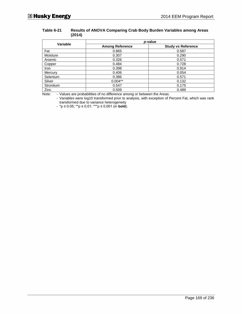
Submitted To 2014 EEM Program Report
Page 169 of 236
Table 6-21 Results of ANOVA Comparing Crab Body Burden Variables among Areas (2014)
Variable p-value
Among Reference Study vs Reference
Fat 0.865 0.587
Moisture 0.307 0.290
Arsenic 0.326 0.571
Copper 0.484 0.728
Iron 0.398 0.914
Mercury 0.406 0.054
Selenium 0.386 0.571
Silver 0.004** 0.132
Strontium 0.547 0.175
Zinc 0.509 0.489
Note: - Values are probabilities of no difference among or between the Areas. - Variables were log10 transformed prior to analysis, with exception of Percent Fat, which was rank
transformed due to variance heterogeneity - *p ≤ 0.05; **p ≤ 0.01; ***p ≤ 0.001 (in bold).

Submitted To 2014 EEM Program Report
Page 170 of 236
Ref1 Ref2 Ref3 Ref4 Study
Area
0.2
0.3
0.4
0.5
0.6
0.7
0.8
0.9
1.0
% F
at
Ref1 Ref2 Ref3 Ref4 Study
Area
80
81
82
83
84
% M
ois
ture
Ref1 Ref2 Ref3 Ref4 Study
Area
0
5
10
15
Ars
enic
(m
g/k
g w
et)
Ref1 Ref2 Ref3 Ref4 Study
Area
4
5
6
7
8
9
Co
pp
er (m
g/k
g w
et)
Ref1 Ref2 Ref3 Ref4 Study
Area
0
5
10
15
Iro
n (
mg
/kg
wet)
Ref1 Ref2 Ref3 Ref4 Study
Area
0.00
0.05
0.10
0.15
0.20
Merc
ury
(m
g/k
g w
et)
Ref1 Ref2 Ref3 Ref4 Study
Area
0.0
0.5
1.0
1.5
Sele
niu
m (
mg
/kg
wet)
Ref1 Ref2 Ref3 Ref4 Study
Area
0.0
0.1
0.2
0.3
0.4
Silv
er (m
g/k
g w
et)
Ref1 Ref2 Ref3 Ref4 Study
Area
0
5
10
15
Str
ontium
(m
g/k
g w
et)
Ref1 Ref2 Ref3 Ref4 Study
Area
0
10
20
30
Zin
c (m
g/k
g w
et)
Figure 6-10 Box Plots of Variable Concentrations in Crab Claw in Reference and Study Areas (2014)
Notes: The centre line is the median. Ends of the box indicate the lower and upper quartiles. Ends of the whiskers indicate the quartile ±1.5 x interquartile spread. Asterisks indicate values falling within the quartile ±3 x interquartile spread. Open circles indicate values falling outside the quartile ±3 x interquartile spread.
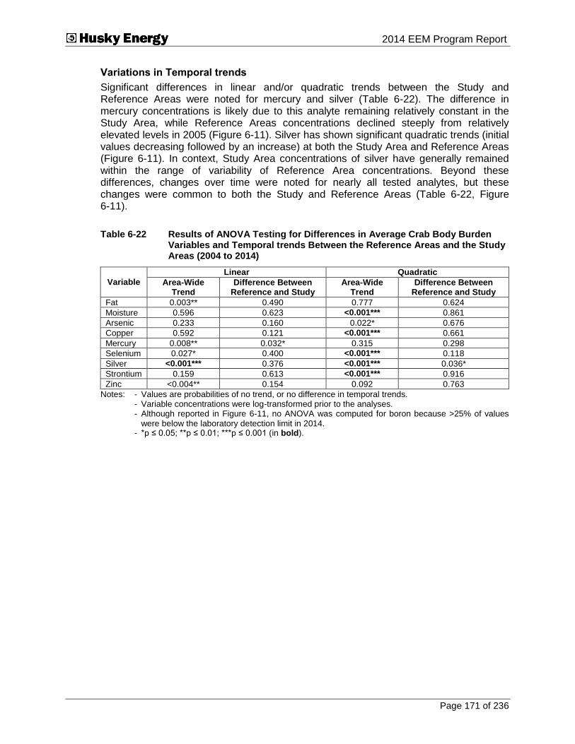
Submitted To 2014 EEM Program Report
Page 171 of 236
Variations in Temporal trends
Significant differences in linear and/or quadratic trends between the Study and Reference Areas were noted for mercury and silver (Table 6-22). The difference in mercury concentrations is likely due to this analyte remaining relatively constant in the Study Area, while Reference Areas concentrations declined steeply from relatively elevated levels in 2005 (Figure 6-11). Silver has shown significant quadratic trends (initial values decreasing followed by an increase) at both the Study Area and Reference Areas (Figure 6-11). In context, Study Area concentrations of silver have generally remained within the range of variability of Reference Area concentrations. Beyond these differences, changes over time were noted for nearly all tested analytes, but these changes were common to both the Study and Reference Areas (Table 6-22, Figure 6-11).
Table 6-22 Results of ANOVA Testing for Differences in Average Crab Body Burden Variables and Temporal trends Between the Reference Areas and the Study Areas (2004 to 2014)
Variable
Linear Quadratic
Area-Wide Trend
Difference Between Reference and Study
Area-Wide Trend
Difference Between Reference and Study
Fat 0.003** 0.490 0.777 0.624
Moisture 0.596 0.623 <0.001*** 0.861
Arsenic 0.233 0.160 0.022* 0.676
Copper 0.592 0.121 <0.001*** 0.661
Mercury 0.008** 0.032* 0.315 0.298
Selenium 0.027* 0.400 <0.001*** 0.118
Silver <0.001*** 0.376 <0.001*** 0.036*
Strontium 0.159 0.613 <0.001*** 0.916
Zinc <0.004** 0.154 0.092 0.763
Notes: - Values are probabilities of no trend, or no difference in temporal trends. - Variable concentrations were log-transformed prior to the analyses. - Although reported in Figure 6-11, no ANOVA was computed for boron because >25% of values
were below the laboratory detection limit in 2014. - *p ≤ 0.05; **p ≤ 0.01; ***p ≤ 0.001 (in bold).

Submitted To 2014 EEM Program Report
Page 172 of 236
Year
0.5
0.6
0.7
0.8
0.9
1.0
1.1
1.2
Perc
ent
Lip
id
Year
60
65
70
75
80
85
Perc
ent
Mo
istu
re
Year
4
5
6
7
8
9
10
11
12
Ars
enic
(m
g/k
g w
et)
Year
1.5
2.0
2.5
3.0
3.5
Bo
ron (m
g/k
g w
et)
Year
2
3
4
5
6
Co
pp
er (m
g/k
g w
et)
Year
0.04
0.08
0.12
0.16
0.20
Merc
ury
(m
g/k
g w
et)
Year
0.5
0.6
0.7
0.8
0.9
1.0
Sele
niu
m (
mg
/kg
wet)
Year
0.12
0.14
0.16
0.18
0.20
0.22
0.24
Silv
er (m
g/k
g w
et)
Year
10
15
20
25
30
Str
ontium
(m
g/k
g w
et)
Year
22
24
26
28
30
32
34
Zin
c (m
g/k
g w
et)
Study
Reference
Figure 6-11 Variation in Area Means of Detectable Variable Concentrations in Crab Claw Composites from 2004 to 2014
Note: Values shown are annual averages within Areas. Red circles are Study Area averages; open circles are averages for each Reference Area.

Submitted To 2014 EEM Program Report
Page 173 of 236
6.2.3 Taste Tests
6.2.3.1 Plaice
No significant difference in taste was noted between plaice from the Study and Reference Areas in 2014 in both the triangle and hedonic scaling tests. Panelists for the triangle test were successful in discriminating 8 out of 24 samples. These results are not
significant at = 0.05 (Appendix C-4). ANOVA statistics for hedonic scaling are provided
in Table 6-23. The results were not significant (p = 0.61; = 0.05) and, from the frequency histogram (Figure 6-12), samples from both the Study and Reference Areas were assessed similarly for preference. From ancillary comments (Tables 6-24 and 6-25, and Appendix C-4), there were no consistent comments identifying abnormal or foreign odour or taste.
Table 6-23 ANOVA for Taste Preference Evaluation of Plaice by Hedonic Scaling (2014)
Source of Variation SS df MS F p-value
Between Groups 0.52 1 0.52 0.26 0.61
Within Groups 91.79 46.00 2.00 Total 92.31 47.00
Note - *p ≤ 0.05; **p ≤ 0.01; ***p ≤ 0.001 (in bold).
0.0
5.0
10.0
15.0
20.0
25.0
30.0
35.0
40.0
45.0
Perc
en
t (%
)
Study Reference
Figure 6-12 Plaice Frequency Histogram for Hedonic Scaling Taste Evaluation (2014)

Submitted To 2014 EEM Program Report
Page 174 of 236
Table 6-24 Summary of Comments from the Triangle Taste Test for Plaice (2014)
Reference Area (RA) Study Area (SA)
Correctly identified as odd sample Correctly identified as odd sample
292 (RA) slightly different but not offensive Sample 271 (SA) has a more preferred flavour
A little difference in odor. No real flavour difference Slightly more salt
More "fishy" taste on sample 292 (RA) I found smell and taste different
Incorrectly identified as odd sample Incorrectly identified as odd sample
Very little difference in samples Hard to tell the difference
807 (RA) was more tasty than the 2 others, which were bland
Just a guess. Too similar! Thanks
Very close in taste; hard to choose Very slight difference
Much blander (and more watery) than others. Stronger flavour. The other samples had a mild flavour
Table 6-25 Summary of Comments from the Hedonic Scaling Taste Test for Plaice (2014)
Preferred Reference Area Preferred Study Area
Mild flavour 520 (SA) was more desirable and had a slightly sweeter flavour
No real difference Too strong taste on sample 110 (RA). Preferred 483 (SA)
Very good 483 (SA) tastes more natural (i.e., no salt added)
110 (RA) slightly more flavour 753 (SA) had a very nice seafood flavour and odour. 992 (RA) smelled good but left an off aftertaste
A bit more flavourful and sweet than 753 (SA) A bit more flavourful and sweet than 753 (SA)
Never found much difference in the two Never found much difference in the two
Both very good flavour, pleasant, no off flavours or odours. Both very similar in terms of flavour and odour
Both very good flavour, pleasant, no off flavours or odours. Both very similar in terms of flavour and odour
Not enough
483 (SA) was a little more bland
6.2.3.2 Crab
No significant difference in taste was noted between crab from the Study and Reference Areas in both the triangle and hedonic scaling tests. Panelists for the triangle test were successful in discriminating 10 out of 24 samples. These results were not significant at
= 0.05 (Appendix C-4). ANOVA statistics for hedonic scaling are provided in Table
6-26. The results were not significant (p = 0.76; = 0.05) and, from the frequency histogram (Figure 6-13), samples from both the Study and Reference Areas were assessed similarly for preference. From ancillary comments (Tables 6-27 and 6-28, and Appendix C-4), there were no consistent comments identifying abnormal or foreign odour or taste.
Table 6-26 ANOVA for Taste Preference Evaluation of Crab by Hedonic Scaling (2014)
Source of Variation SS df MS F p-value
Between Groups 0.19 1.00 0.19 0.09 0.76
Within Groups 91.29 46.00 1.98 Total 91.48 47.00
Note - *p ≤ 0.05; **p ≤ 0.01; ***p ≤ 0.001 (in bold).

Submitted To 2014 EEM Program Report
Page 175 of 236
0.0
5.0
10.0
15.0
20.0
25.0
30.0
35.0
40.0
45.0
Pe
rce
nt
(%)
Study Reference
Figure 6-13 Crab Frequency Histogram for Hedonic Scaling Taste Evaluation (2014)
Table 6-27 Summary of Comments from the Triangle Taste Test for Crab (2014)
Reference Area (RA) Study Area (SA)
Correctly identified as odd sample Correctly identified as odd sample
I couldn't determine much of a difference Quite similar taste and odour for all samples
Didn't really taste any difference 565 (SA) seems to have a slightly stronger crab taste than the other two. 263 (RA) and 701 (RA) were slightly unpalatable
458 (SA) too crunchy
Stronger crab taste. Other 2 samples are blander
Very difficult to choose - all very similar in taste
Incorrectly identified as odd sample Incorrectly identified as odd sample
Definitely - smelled nicer too No real difference
Tastes sweeter and more fresh Very difficult to tell any difference; I guessed at 458 (SA)
Slight off flavour on 263 (RA) Tasted off compared to others; not as sweet
All samples were similar
Very little difference

Submitted To 2014 EEM Program Report
Page 176 of 236
Table 6-28 Summary of Comments from Hedonic Scaling Taste Tests for Crab (2014)
Preferred Reference Area Preferred Study Area
No difference No difference
311 (RA) has a sweeter flavour while 631 (SA) was saltier
315 (SA) - strong odour but more flavour than 469 (RA)
Slight difference; 631 (SA) was a little more sour tasting
No real difference
No significant difference between the two samples They both taste and smell good
No real difference 368 (SA) sweeter taste
More flavour on sample 433 (RA) 368 (SA) was a little for flavourful
433 (RA) tasted sweeter Liked the smell of 671 (SA) more than 507 (RA). 671 (SA) had a nice seafood smell
Pleasant, sweet characteristic, OK. The homogenous state takes away from the overall appeal
507 (RA) tastes little sweeter but very good
6.2.4 Fish Health
6.2.4.1 Gross Pathology
No visible abnormalities were observed upon necropsy on the skin or fins of fish or on the external surface of the gonad, digestive tract, liver, body-cavity or spleen (Appendix C-3, Annex C).
6.2.4.2 Haematology
Blood smears collected during the 2014 survey displayed signs of clotting, water micro-droplets and lack of uniformity. Therefore, they were considered not suitable for carrying out reliable differential cell counts. Preliminary screening of the smears indicated that counts could vary by more than 20% upon examination of different regions of a slide. In human haematology, when 200 cells are counted, the variability is normally in the ±7 to 10% range (Lynch et al. 1969). Oceans Ltd. considered the quality of smears poor and the variability too high in the 2014 fish for carrying out haematological analysis.
6.2.4.3 Mixed Function Oxygenase Activity
No significant differences were found in hepatic EROD activity among Reference Areas for pre-spawning and spent females (p = 0.416 and 0.882, respectively). EROD activity was significantly lower in pre-spawning and spent female fish from the Study Area relative to fish from the combined Reference Areas (p = 0.009 and 0.024, respectively; Figure 6-14, Table 6-29). The mean ± standard deviation of pre-spawning females from the combined Reference Areas was 15.48 ± 9.89 pmol/min/mg protein, while that of fish from the Study Area was 11.39 ± 9.80 pmol/min/mg protein. For spent females, the mean ± standard deviation of the pre-spawning females from the combined Reference Areas was 18.13 ± 11.86 pmol/min/mg protein, while that of females from the Study Area was 8.49 ± 6.64 pmol/min/mg protein.
Too few male or immature female fish were captured to allow for statistical comparisons.

Submitted To 2014 EEM Program Report
Page 177 of 236
Area
01020304050607080
pm
ol/
min
/mg
pro
tein
Area
01020304050607080
pm
ol/
min
/mg
pro
tein
Figure 6-14 Box Plots of EROD Activity in the Liver of: Top) Pre-spawning (F-510 to F-540); and Bottom) Spent (F-550 to F-580) Female Plaice
Notes: The centre line is the median. Ends of the box indicate the lower and upper quartiles. Ends of the whiskers indicate the quartile ±1.5 x interquartile spread. Asterisks indicate values falling within the quartile ±3 x interquartile spread. Open circles indicate values falling outside the quartile ±3 x interquartile spread.
See Appendix C-3, Annex A for DFO maturity stage classifications.
Table 6-29 Results of ANOVA Comparing EROD Activities in Female Plaice (2014)
Variable (Y) p-value
Among References Study versus References
Pre-Spawn Females 0.416 0.009**
Spent Females 0.883 0.024*
Notes: - EROD activities were log-transformed. - *p ≤ 0.05; **p ≤ 0.01; ***p ≤ 0.001 (in bold).
- * See Appendix C-3, Annex A for maturity stage classifications.
6.2.4.4 Histopathology
Liver Histopathology
Results of liver histopathology expressed as the percentage of fish affected by each type of lesion/observation (or prevalence of lesion) in each Area are provided in Table 6-30. The complete data set is provided in Appendix C-3, Annex F. Representative photographs of normal liver as well as a number of histological changes are included in Appendix C-3, Annex H.
A B

Submitted To 2014 EEM Program Report
Page 178 of 236
Table 6-30 Number and Frequency of Plaice with Specific Types of Hepatic Lesions and Prevalence of Lesions (2014)
Hepatic Lesions Measure Area
Ref 1 Ref 2 Ref 3 Ref 4 All Ref Study Total
Number of Fish Number 30 30 30 30 120 60 180
Nuclear Pleomorphism Number 0 0 0 0 0 0 0
% 0 0 0 0 0.00 0
Megalocytic Hepatosis Number 0 0 0 0 0 0 0
% 0 0 0 0 0.00 0
Focus of cellular alteration Number 0 0 0 0 0 0 0
% 0 0 0 0 0.00 0
Proliferation of Macrophage Aggregates a
Number 7 13 16 15 51 35 86
% 23.33 43.33 53.33 50 42.50 58.33
Fibrillar Inclusions Number 0 0 0 0 0 0 0
% 0 0 0 0 0.00 0
Inflammatory Response b Number 0 0 0 0 0 0 0
% 0 0 0 0 0.00 0
Hepatocellular Vacuolation Number 1 1 0 1 3 2 5
% 3.33 3.33 0 3.33 2.50 3.33
Parasites Number 7 7 14 1 29 15 44
% 23.33 23.33 46.66 3.33 24.17 50
Golden Rings Number 0 0 0 1 1 2 3
% 0 0 0 3.33 0.83 3.33
Notes: - a Defined as scores greater than 3 on a 0-7 relative scale. - b Inflammation response including mild, moderate and severe scores.
No cases of nuclear pleomorphism, megalocytic hepatosis, focus of cellular alteration, fibrillar inclusions, or inflammatory response were detected in any of the fish. Five cases of hepatocellular vacuolation were detected, two in the Study Area and one in each of Reference Areas 1, 2 and 4. Proliferation of macrophage aggregates was detected in 86 fish, 35 from the Study Area and in 7, 13, 16 and 15 fish from Reference Areas 1, 2, 3 and 4, respectively, with one fish from Reference Area 3 showing a severe case of macrophage aggregation. Although such liver conditions are of interest, they are generally not a result of the presence of chemical pollutants17.
Golden rings were detected around bile ducts in two fish from the Study Area and one fish from Reference Area 4. The rings are most likely melanization at the margin of the bile duct.
Statistical analyses were conducted on macrophage aggregates and parasites only since the low incidence of all the other hepatic lesions prevented statistical comparisons. Overall, there were no significant differences in either biliary parasites (Fisher exact test, p = 1.00) or macrophage aggregates (Fisher exact test, p = 0.258) between fish from the Study and Reference Areas.
17 In addition to observations in association with toxicity, melano-macrophage aggregate proliferation has also been associated with infectious diseases and parasite infestation (Roberts 1989), starvation and nutritional imbalance (Agius 1979a; Agius and Roberts 1981) and ageing (Agius 1979b; Brown and George 1985). Due to the varied influences on the proliferation of melano-macrophage aggregates, its presence is considered a non-specific lesion according to the BEQUALM categories of histopathological lesions in fish that should be used in PAH-specific biological effects monitoring (OSPAR Convention Monitoring Guidelines 1998).

Submitted To 2014 EEM Program Report
Page 179 of 236
Gill Histopathology
Accurate gill histopathology counts were not possible for one fish from the Reference Area 3, two fish from Reference Area 4 and three fish from the Study Area. Detailed histopathological counts were thus carried out on gill tissues of 117 fish from the Reference Areas and 57 fish from the Study Area. In all cases, the frequencies of lamellae affected by the lesions were very low; all were less than 0.002%, except for one fish from Reference 3 with 21.30% of lamellae exhibiting telangiectasis. Representative photographs of gill slides used during the analysis can be found in Appendix C-3, Annex H.
Means ± standard deviation of frequencies of lamellae presenting each type of lesion per site are provided in Table 6-31.
Statistical comparisons were carried out on the number of fish exhibiting lesions between the Study Area versus the combined Reference Areas (Table 6-32) using Fisher’s Exact Test. Lesions were considered “present” if occurring on any of the lamellae examined for each fish. None of the gill lesions occurred either more or less frequently in Study Area fish compared to Reference Area fish (Fisher Exact test, p > 0.05 in all cases).

Submitted To 2014 EEM Program Report
Page 180 of 236
Table 6-31 Occurrence of Lesions in the Gill Tissues of Plaice (2014)
Gill Lesions
Area
Reference 1 Reference 2 Reference 3 Reference 4 Study Total
Number of Fish 30 30 29 28 57 174
Distal Hyperplasia a 0.0409 ± 0.1306 0.0769 ± 0.2735 0.0304 ± 0.0742 0.0463 ± 0.091 0.0501 ± 0.1441 0.0493 ± 0.1565
Tip Hyperplasia a 0.065 ± 0.1736 0.0932 ± 0.1769 0.061 ± 0.12 0.0946 ± 0.1721 0.0794 ± 0.1399 0.0787 ± 0.1541
Basal Hyperplasia 1a b 0.1425 ± 0.5884 0.0268 ± 0.0833 0.1352 ± 0.3077 0.133 ± 0.2725 0.176 ± 0.7914 0.1308 ± 0.5398
Basal Hyperplasia 2 a c 0.0924 ± 0.3193 0.012 ± 0.066 0.0076 ± 0.0412 0.0172 ± 0.0633 0.0212 ± 0.1601 0.029 ± 0.167
Fusion a 0.0626 ± 0.2442 0.029 ± 0.0906 0.0354 ± 0.1099 0.0087 ± 0.0461 0.0776 ± 0.2634 0.0485 ± 0.1918
Telangiectasis a 0.0041 ± 0.0224 0.0089 ± 0.0337 0 0 0.0075 ± 0.0564 0.0047 ± 0.0363
Notes: - Values are means 1 standard deviation. - a Mean frequency (%) of lamellae presenting the lesion. - b Basal hyperplasia 1: increase in thickness of the epithelium reaching 1/3 to 2/3 of total lamellar length. - c Basal hyperplasia 2: increase in thickness of the epithelium reaching more than 2/3 of total lamellar length.

Submitted To 2014 EEM Program Report
Page 181 of 236
Table 6-32 Number of Plaice with Specific Types of Gill Lesions and Percentages of Fish Exhibiting the Lesions (2014)
Gill Lesions Measure
Area
Ref 1 Ref 2 Ref 3 Ref 4 Reference
Mean Study
Number of Fish Number 30 30 29 28 29 57
Distal Hyperplasia Number 4 5 5 7 5 11
% 13 17 17 25 18 19
Tip Hyperplasia Number 7 8 9 11 9 19
% 23 27 31 39 30 33
Basal Hyperplasia 1 a Number 4 3 8 7 6 11
% 13 10 28 25 19 19
Basal Hyperplasia 2 b Number 3 1 1 2 2 1
% 10 3 3 7 6 2
Fusion Number 2 3 3 1 2 8
% 7 10 10 4 8 14
Telangiectasis Number 1 2 0 0 1 1
% 3 7 0 0 3 2
Notes: - Hyperplasia and fusion were considered “present” if those conditions occurred on any of the lamellae examined for each fish.
- a Basal hyperplasia 1: increase in thickness of the epithelium reaching 1/3 to 2/3 of total lamellar
length. - b Basal hyperplasia 2: increase in thickness of the epithelium reaching more than 2/3 of total
lamellar length.
6.3 Summary of Results
6.3.1 Biological Characteristics
There was no significant difference in mean gutted weight between the Reference Area composites and Study Area composites for plaice used in body burden analyses. There were significant differences in measures of crab size (carapace width and claw height) between the Study Area and the Reference Areas, and among the Reference Areas. In general, crab from Reference Area 3 and the Study Area were slightly smaller than crab from Reference Area 2 and 4.
Difference among Areas in plaice maturity stage, length, gutted weight, age, gutted weight (corrected for length) and liver weight and gonad weight (corrected for gutted weight) were also examined within the context of fish health analyses. Only one male was captured, and almost all of the females examined (215 of 219 females, or 98%) were mature. Of the mature females, 90% were pre-spawning and the remainder were spent. The frequency of pre-spawning mature females was lower in the Reference Areas compared to the Study Area (85% versus 93%, respectively). Fish length and gutted weight did not vary significantly between the Study and Reference Areas. Pre-spawning females from the Study Area were significantly older, and both pre-spawning and spent females from the Study Area had greater gonad weight relative to Reference Areas. Significant differences between the Study and Reference Areas in pre-spawning female liver weight relative to gutted weight were also noted; fish from Reference Area 2 had smaller livers.
Submitted To 2014 EEM Program Report
Page 182 of 236
6.3.2 Body Burden
In 2014, most frequently detected compounds in plaice liver (arsenic, copper, iron, manganese, selenium, strontium, >C10-C21) did not vary significantly in concentration between the Study and Reference Areas. However, percent fat and concentrations of >C21-C32 hydrocarbons were significantly lower in the Study Area; percent moisture and concentrations of cadmium and zinc were significant higher in the Study Area.
Compounds in the >C10-C21 and >C21-C32 hydrocarbon range were again detected in all liver samples in 2014. As in previous years, additional Gas Chromatography/Mass Spectrometer analysis did not indicate the presence of drill fluid or petroleum hydrocarbons in those samples.
There were no significant differences between the Study Area and the Reference Areas in trends over time (2004 to 2014) for most frequently detected compounds in liver. However, a difference in linear trend over time between the Reference Areas and the Study Area was observed for percent moisture, with marginally higher concentrations in the Study Area across all years. There was also a significant difference in quadratic trends over time (increase followed by a decrease, or vice versa) between the Study and Reference Areas for >C21-C32 hydrocarbon concentrations, likely influenced by lower concentrations in the Reference Areas in 2006 and 2010.
For plaice fillets in 2014, there were no significant differences in percent fat, moisture, arsenic, iron, mercury, strontium and zinc content between the Study Area and the Reference Areas. There were also no significant differences between the Study Area and the Reference Areas in trends over time (2004 to 2014), except for a significant difference in linear trends in zinc. Further examination of the data indicated that this difference was a statistical artefact, and the more appropriate quadratic function (given the area-wide decreases and subsequent increases in zinc) showed no difference between the Reference and Study Areas.
For crab tissue in 2014, there were no significant differences between the Study Area and the Reference Areas for frequently detected compounds (percent fat, percent moisture, arsenic, copper, iron, mercury, selenium, silver, strontium and zinc). Across years, significant differences in linear and/or quadratic trends between the Study and Reference Areas were noted for silver and mercury. Mercury concentrations remained relatively constant in the Study Area, while Reference Areas concentrations declined steeply from elevated levels in 2005. Silver has shown significant quadratic trends (initial values decreasing followed by an increase) at both the Study Area and Reference Areas (Figure 6-11). However, Study Area concentrations of silver have generally remained within the range of variability of Reference Area concentrations.
6.3.3 Taste Tests
There were no significant differences in taste test results between Study and Reference Areas plaice or crab. From ancillary comments, there were no consistent comments identifying abnormal or foreign odour or taste.
Submitted To 2014 EEM Program Report
Page 183 of 236
6.3.4 Fish Health Indicators
The results of the fish health survey carried out in 2014 indicated that the overall health of American plaice is similar between the Reference Areas and the Study Area, as assessed by a number of bioindicator responses. Although EROD activity was significantly lower in pre-spawning and spent female fish from the Study Area relative to fish from the Reference Areas, no visible abnormalities were observed upon necropsy on the skin or fins of fish or on the external surface of the gonad, digestive tract, liver, body-cavity, or spleen. Incidences of hepatic lesions were low in all Areas, and no significant differences between the Study and Reference Areas were noted in either biliary parasites or in liver macrophage aggregates. Incidence of gill lesions also did not differ between the Study and the Reference Areas.
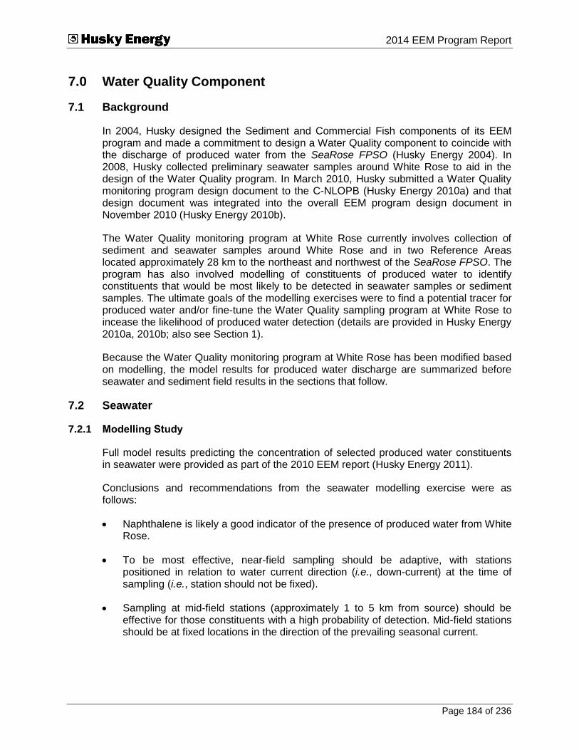
Submitted To 2014 EEM Program Report
Page 184 of 236
7.0 Water Quality Component
7.1 Background
In 2004, Husky designed the Sediment and Commercial Fish components of its EEM program and made a commitment to design a Water Quality component to coincide with the discharge of produced water from the SeaRose FPSO (Husky Energy 2004). In 2008, Husky collected preliminary seawater samples around White Rose to aid in the design of the Water Quality program. In March 2010, Husky submitted a Water Quality monitoring program design document to the C-NLOPB (Husky Energy 2010a) and that design document was integrated into the overall EEM program design document in November 2010 (Husky Energy 2010b).
The Water Quality monitoring program at White Rose currently involves collection of sediment and seawater samples around White Rose and in two Reference Areas located approximately 28 km to the northeast and northwest of the SeaRose FPSO. The program has also involved modelling of constituents of produced water to identify constituents that would be most likely to be detected in seawater samples or sediment samples. The ultimate goals of the modelling exercises were to find a potential tracer for produced water and/or fine-tune the Water Quality sampling program at White Rose to incease the likelihood of produced water detection (details are provided in Husky Energy 2010a, 2010b; also see Section 1).
Because the Water Quality monitoring program at White Rose has been modified based on modelling, the model results for produced water discharge are summarized before seawater and sediment field results in the sections that follow.
7.2 Seawater
7.2.1 Modelling Study
Full model results predicting the concentration of selected produced water constituents in seawater were provided as part of the 2010 EEM report (Husky Energy 2011).
Conclusions and recommendations from the seawater modelling exercise were as follows:
Naphthalene is likely a good indicator of the presence of produced water from White Rose.
To be most effective, near-field sampling should be adaptive, with stations positioned in relation to water current direction (i.e., down-current) at the time of sampling (i.e., station should not be fixed).
Sampling at mid-field stations (approximately 1 to 5 km from source) should be effective for those constituents with a high probability of detection. Mid-field stations should be at fixed locations in the direction of the prevailing seasonal current.

Submitted To 2014 EEM Program Report
Page 185 of 236
Aside from biological/chemical reactivity and physical properties, the probability of detection of a constituent is dictated by its release concentration and its laboratory detection limit. Therefore, the lowest reliable detection limit should be used for the analysis of field samples.
Recommendations were first implemented for the 2012 field program and continue to be implemented.
7.2.2 Field Sampling
7.2.2.1 Water Sample Collection
Water collection for the 2014 EEM Program was conducted from November 4 to November 5, 2014, using the offshore supply vessel Atlantic Raven. Collection stations for the 2014 program are shown in Figure 7-1. In accordance with recommendations in Section 7.2.1, samples in the near-field were collected down-current from the SeaRose FPSO. In 2014, those stations were located to the northeast of the SeaRose FPSO. Station coordinates and distance to the SeaRose FPSO are provided in Appendix D-1.
Water samples were collected at 10 m below surface (“surface”), 40 m below surface (“mid-depth”), and 10 m above bottom (“bottom”) using a string of three Teflon-lined, 10 L Niskin-X bottle water samplers (Figure 7-2). All stations were sampled for physical and chemical characteristics. Compounds analyzed included BTEX (benzene, toluene, ethylbenzene, and xylenes) hydrocarbons, >C10-C21 and >C21-C32 hydrocarbons, PAHs (polycyclic aromatic hydrocarbons) and alkyl PAHs, phenols and alkyl phenols, volatile organic acids, metals, total inorganic and organic carbon (TIC and TOC, respectively), total suspended solids (TSS) and ammonia. Samples were stored as detailed in Table 7-1.
A conductivity, temperature, depth (CTD) recorder cast was performed at all Water Quality stations to assess the depth of the thermocline relative to Niskin bottle sample location.
Field blanks for BTEX, >C10-C21 and >C21-C32 hydrocarbons, PAHs and alkyl PAHs, phenols and alkyl phenols, organic acids, metals and ammonia were collected at stations 4 (mid-depth), W-2NE (surface), W-5NE (mid-depth) and W-16R (mid-depth). Duplicate samples were collected at the same stations. Field blanks indicated no contamination from the field collection environment and duplicate samples provided similar results to the field sample (see Appendix D-2 – Results).
7.2.2.2 Laboratory Processing
Water samples were processed for constituents listed in Table 7-2. In the 2010 EEM program, most constituents were processed at RPC, Fredericton, NB. In 2012 and 2014, inorganic constituents (trace metals, mercury) were processed at Maxxam Analytics (Halifax, NS) because detection limits for most inorganic constituents of interest were lower at that analytical laboratory, as per recommendations in Section 7.2.1. TIC/TOC/TSS and ammonia were also processed at Maxxam Analytics in 2012 and 2014. The remaining constituents were processed at RPC. Details on analytical methods for RPC and Maxxam Analytics are provided in Appendix D-2.
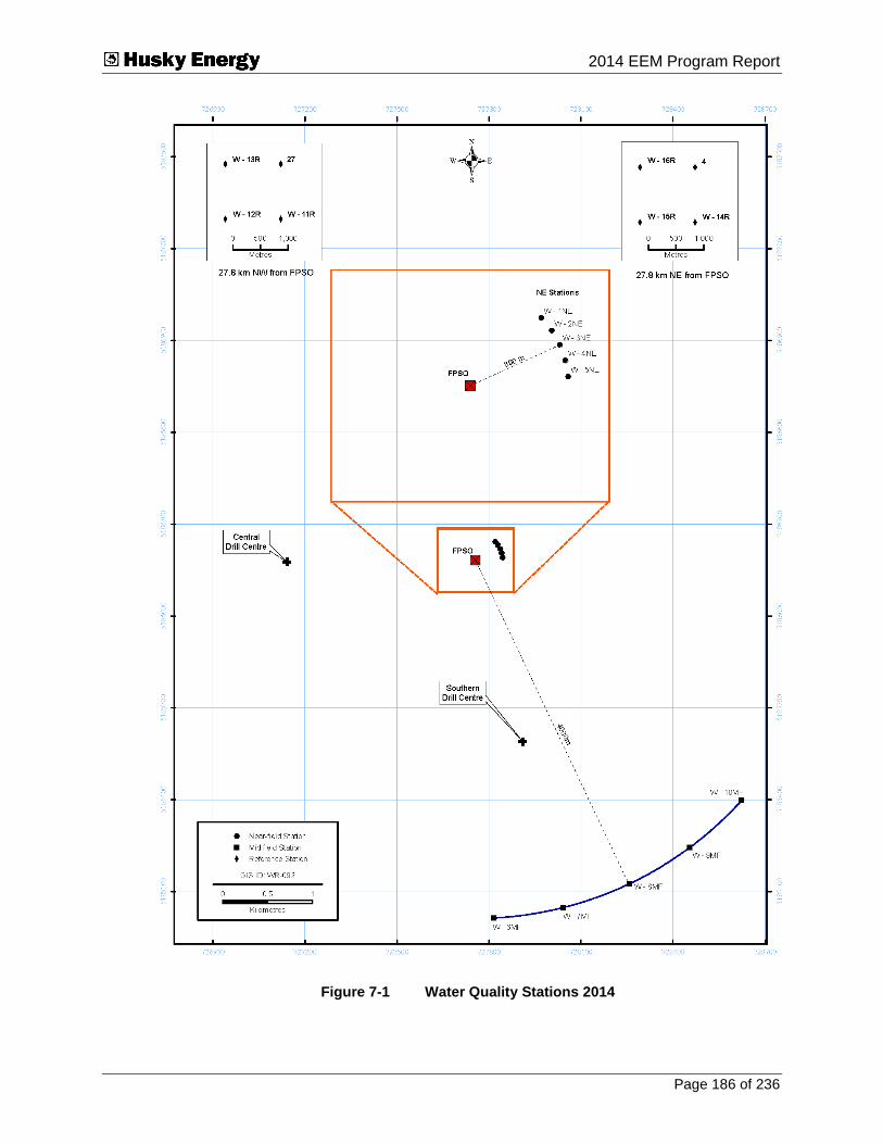
Submitted To 2014 EEM Program Report
Page 186 of 236
Figure 7-1 Water Quality Stations 2014
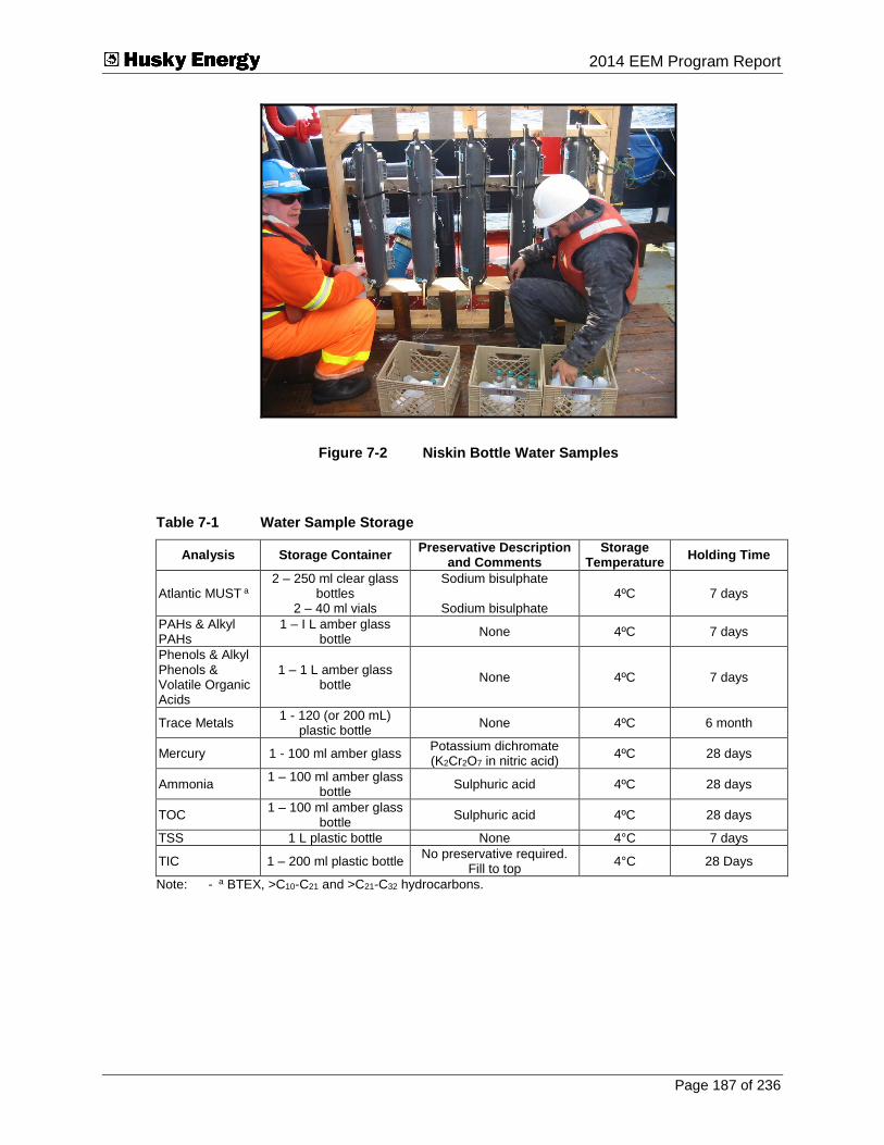
Submitted To 2014 EEM Program Report
Page 187 of 236
Figure 7-2 Niskin Bottle Water Samples
Table 7-1 Water Sample Storage
Analysis Storage Container Preservative Description
and Comments Storage
Temperature Holding Time
Atlantic MUST a 2 – 250 ml clear glass
bottles 2 – 40 ml vials
Sodium bisulphate
Sodium bisulphate 4ºC 7 days
PAHs & Alkyl PAHs
1 – I L amber glass bottle
None 4ºC 7 days
Phenols & Alkyl Phenols & Volatile Organic Acids
1 – 1 L amber glass bottle
None 4ºC 7 days
Trace Metals 1 - 120 (or 200 mL)
plastic bottle None 4ºC 6 month
Mercury 1 - 100 ml amber glass Potassium dichromate (K2Cr2O7 in nitric acid)
4ºC 28 days
Ammonia 1 – 100 ml amber glass
bottle Sulphuric acid 4ºC 28 days
TOC 1 – 100 ml amber glass
bottle Sulphuric acid 4ºC 28 days
TSS 1 L plastic bottle None 4°C 7 days
TIC 1 – 200 ml plastic bottle No preservative required.
Fill to top 4°C 28 Days
Note: - a BTEX, >C10-C21 and >C21-C32 hydrocarbons.

Submitted To 2014 EEM Program Report
Page 188 of 236
Table 7-2 Water Chemistry Constituents (2010, 2012 and 2014)
Constituent Unit Detection Limit
2010 2012 2014
Hydrocarbons
Benzene mg/L 0.001 0.001 0.001
Toluene mg/L 0.001 0.001 0.001
Ethylbenzene mg/L 0.001 0.001 0.001
Xylenes mg/L 0.001 0.001 0.001
C6-C10 (less BTEX) mg/L 0.01 0.01 0.01
>C10-C21 mg/L 0.05 0.05 0.05
>C21-C32 mg/L 0.1 0.1 0.1
Phenols and Alkyl Phenols
Phenol µg/L 10 10 10
o-cresol µg/L 10 10 10
m,p-cresol µg/L 10 10 10
Total C2 Phenols µg/L 20 20 20
Total C3 Phenols µg/L 20 20 20
Total C4 Phenols µg/L 20 20 20
Total C5 Phenols µg/L 20 20 20
4-n-hexylphenol µg/L 10 10 10
2,5-diisopropylphenol µg/L 10 10 10
2,6-diisopropylphenol µg/L 10 10 10
2-tert-butyl-4-ethylphenol µg/L 10 10 10
6-tert-butyl-2,4-dimethyphenol µg/L 10 10 10
4-n-heptylphenol µg/L 10 10 10
2,6-dimethyl-4-(1,1-dimethypropyl) phenol µg/L 10 10 10
4-(1-ethyl-1-methylpropyl)-2-methylphenol µg/L 10 10 10
4-n-octylphenol µg/L 10 10 10
4-tert-octylphenol µg/L 10 10 10
2,4-di-sec-butylphenol µg/L 10 10 10
2,6-di-tert-butylphenol µg/L 10 10 10
4-n-nonylphenol µg/L 20 20 20
2-methyl-4-tert-octylphenol µg/L 10 10 10
2,6-di-tert-butyl-4-methylphenol µg/L 10 10 10
4,6-di-tert-butyl-2-methylphenol µg/L 10 10 10
PAHs and Alkyl PAHs
Naphthalene µg/L 0.01 0.05 0.05
Acenaphthylene µg/L 0.01 0.01 0.01 Acenaphthene µg/L 0.01 0.01 0.01 Fluorene µg/L 0.01 0.01 0.01 Phenanthrene µg/L 0.01 0.01 0.01 Anthracene µg/L 0.01 0.01 0.01 Fluoranthene µg/L 0.01 0.01 0.01 Pyrene µg/L 0.01 0.01 0.01 Benzo(a)anthracene µg/L 0.01 0.01 0.01 Chrysene/Triphenylene µg/L 0.01 0.01 0.01 Benzo(b)fluoranthene µg/L 0.01 0.01 0.01 Benzo(k)fluoranthene µg/L 0.01 0.01 0.01 Benzo(e)pyrene µg/L 0.01 0.01 0.01 Benzo(a)pyrene µg/L 0.01 0.01 0.01 Indenopyrene µg/L 0.01 0.01 0.01 Benzo(g,h,i)perylene µg/L 0.01 0.01 0.01 Dibenzo(a,h)anthracene µg/L 0.01 0.01 0.01 C1-Naphthalenes a µg/L 0.05 0.10 0.10
C2-Naphthalenes a µg/L 0.05 0.10 0.10 C3-Naphthalenes µg/L 0.05 0.10 0.10 C1-Phenanthrenes µg/L 0.05 0.10 0.10 C2-Phenanthrenes µg/L 0.05 0.10 0.10 C3-Phenanthrenes µg/L 0.05 0.10 0.10 Dibenzothiophene µg/L 0.05 0.10 0.10 C1-Dibenzothiophenes µg/L 0.05 0.10 0.10 C2-Dibenzothiophenes µg/L 0.05 0.10 0.10 C3-Dibenzothiophenes µg/L 0.05 0.10 0.10 Perylene µg/L 0.01 0.01 0.01
Biphenyl µg/L 0.01 0.05 0.05

Submitted To 2014 EEM Program Report
Page 189 of 236
Constituent Unit Detection Limit
2010 2012 2014
Organic Acids
Acetic Acid mg/L 2 2 2
Propionic Acid mg/L 2 2 2
Iso-butyric Acid mg/L 2 2 2
Butyric Acid mg/L 2 2 2
Iso-valeric Acid mg/L 2 2 2
n-valeric Acid mg/L 2 2 2
Radionuclides b
Radium-228 Bq/L 1 NA NA
Radium-226 Bq/L 0.3 NA NA
Lead-210 Bq/L 1 NA NA
Metals
Aluminum µg/L 5 10 10
Antimony µg/L 1 0.5 0.5
Arsenic µg/L 10 0.5 0.5
Barium µg/L 0.1 1 1
Beryllium µg/L 0.05 1 1
Boron µg/L 10 50 50
Cadmium µg/L 0.05 0.05 0.05
Calcium mg/L 0.05 1 1
Chromium µg/L 2 0.5 0.5
Cobalt µg/L 0.5 0.10 0.10
Copper µg/L 5 0.5 0.5
Iron µg/L 10 5 5
Lanthanum µg/L 0.2 NA NA
Lead µg/L 0.05 0.1 0.1
Lithium µg/L 5 20 20
Magnesium mg/L 10 1 1
Manganese µg/L 0.01 0.50 0.50
Mercury µg/L 0.025 0.013 0.013
Molybdenum µg/L 0.1 1.0 1.0
Nickel µg/L 5 0.20 0.20
Potassium mg/L 20 1 1
Phosphorus µg/L NA 50 50
Selenium µg/L 10 0.5 0.5
Silicon µg/L NA 100 100
Silver µg/L 0.02 0.05 0.05
Sodium mg/L 0.05 1 1
Strontium µg/L 10 10 10
Sulfur mg/L 0.05 20 20
Tellurium µg/L 0.5 NA NA
Thallium µg/L 2 0.10 0.10
Tin µg/L NA 1.0 1.0
Titanium µg/L NA 10 10
Uranium µg/L 0.1 0.05 0.05
Vanadium µg/L 1 10 10
Zinc µg/L 1 1 1
Other
Unionized Ammonia mg/L NA 0.0001 0.0001
TIC mg/L 0.5 0.5 0.5
TOC mg/L 0.5 5 5
TSS mg/L 5 0.5 0.5
XCide450 mg/L 0.5 0.5 NA
SCW4453 mg/L 1 0.03 NA
Note: - a Includes 1- and 2-Chloronaphthalene. - b Radionuclide sampling was discontinued in 2012 based on model results that showed that
probability of detection in water samples was zero (Husky Energy 2011). - Measurement of the process chemicals XCide450 and SCW4453 was discontinued in 2014 in
accordance with recommendations in the 2012 EEM report (Husky Energy 2013).

Submitted To 2014 EEM Program Report
Page 190 of 236
7.2.2.3 Data Analysis
General Water Quality
Data analyses focused on 2014 data, with qualitative and quantitative comparisons to results from 2010 and 2012. Data collected during baseline (2000) are not comparable to EEM data because the Water Quality monitoring program at White Rose measures a greater number of constituents, many at lower laboratory detection limits, than in 2000. Similarly, preliminary data collected in 2008 are not discussed here because not all constituents were measured at all depths. Data from 2000 and 2008 are reported in Husky Energy (2001) and Husky Energy (2010a).
In 2014, the Water Quality component of the White Rose EEM program used a multiple-Reference and multiple Study Area design, with two Reference Areas and one near-field and one mid-field Study Area. Boxplots of variables that occurred above laboratory detection limit in all or most cases were generated for each Area. Values below detection limit were set to ½ detection limit for plotting.
Overall Area differences were tested on frequently detected variables using ANOVA with Depth and Area as factors. When no significant Area x Depth interaction was detected, the ANOVA was repeated excluding the Area x Depth interaction term from the model, with levels of significance for the factors Area and Depth reported as such. If overall Area differences were significant, then Study versus Reference (S vs R), near-field versus Reference (NF vs R) and mid-field versus Reference (MF vs R) contrasts were examined. One variable with significant Area differences also showed a significant Area x Depth interaction (Section 7.2.2.4); therefore, contrasts were examined within each level of the depth factor (surface, mid-depth and bottom).
Analyses were performed using Systat (version 13). Frequently detected variables with values less than laboratory detection limit were rank transformed before analysis. Rank transformation treats values below detection limit as tied for the lowest rank. Remaining variables were log10 transformed.
Produced Water Constituents
Concentrations of produced water constituents were compared to concentrations at Reference Area stations to generate an estimate of expected enrichment, or depletion, on release resulting from produced water. Individual stations in the near- or mid-field were then examined for produced water constituents with expected concentrations on release more than, or less than, 10 times seawater concentrations. The concentration of produced water constituents was obtained from a produced water chemical characterization performed on a sample collected on November 4, 2014, coincident with water quality sampling.

Submitted To 2014 EEM Program Report
Page 191 of 236
7.2.2.4 Results
General Water Quality
Raw data and summary statistics for analytes measured in seawater samples (Table 7-2) are provided in Appendix D-2. Conductivity, temperature, depth profiles are provided in Appendix D-3. The beginning of the thermocline was at approximately 20 m in the near-field and at most mid-field stations. Temperature readings were unavailable for mid-field stations W6-MF and W10-MF above 30 to 40 m. Therefore, the beginning of the thermocline cannot be located for these two stations. Reference Area stations tended to be more variable, with the beginning of the thermocline between approximately 10 and 20 m.
In 2014, arsenic, barium, boron, calcium, lithium, magnesium, mercury, molybdenum, potassium, sodium, strontium, sulphur, uranium, TIC and ammonia were detected in all samples. TSS was above detection limit in 87% of samples, and nickel was above detection in 81% of samples. With the exception of TIC, which varied over the narrow range of 26 and 28 mg/L, all these variables were included in quantitative analyses for 2014. Of the variables analyzed, most were also frequently detected in 2012. Mercury was not detected in any sample in 2012 and ammonia was only detected in 20% of samples in 2012 (Husky Energy 2013).
The following parameters were not included in quantitative analyses because they were detected in less than 50% of the samples: silicon; cadmium; zinc; iron; lead; copper; silver; thallium; benzene; toluene; silver; >C10-C21 and >C21-C32 hydrocarbons; PAHs and alkyl PAHs; phenols and alkyl phenols; organic acids; and TOC. Silicon was detected in 39% of samples in 2014 (in 10 out of 30 samples from the Study Area and 11 out of 24 samples in the Reference Areas). Cadmium was detected in 26% of samples (in 10 out of 30 samples from the Study Areas and 4 out of 24 samples from the Reference Areas). Zinc was detected in 17% of samples (in five samples from the Study Area and four samples from the Reference Areas). Iron was detected in 9% of samples (in two samples from the Study Areas and two samples from the Reference Areas). Lead was detected in 6% of samples (in two samples from the Study Areas and one sample from the Reference Areas). Copper, silver, thallium, benzene and toluene each were detected in 2% of samples. Copper, thallium, and low levels of benzene and toluene were detected in one sample from the near-field Study Area. Silver was detected in one sample from the mid-field Study Area. >C10-C21 and >C21-C32 hydrocarbons, PAHs and alkyl PAHs, phenols and alkyl phenols and organic acids were not detected in water samples.
Boxplots by area and depth for variables with most values above the laboratory detection limit are provided in Figure 7-3. Boxplots are not provided for TIC because values varied over a very narrow range. The concentration of many metals increased with depth, as in previous years (Husky Energy 2011, 2013). Ammonia decreased with depth (Figure 7.3, Table 7-3).
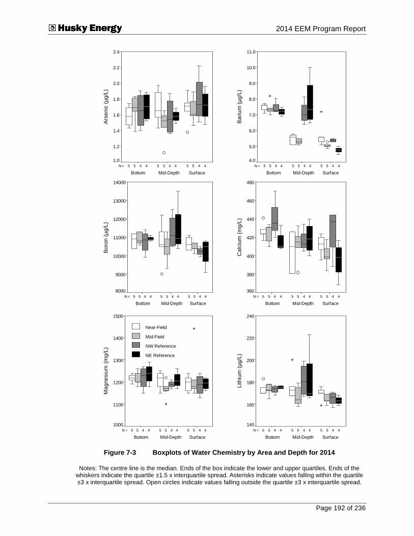
Submitted To 2014 EEM Program Report
Page 192 of 236
444 444 555 555N =
SurfaceMid-DepthBottom
Ars
enic
(µ
g/L
)
2.4
2.2
2.0
1.8
1.6
1.4
1.2
1.0444 444 555 555N =
SurfaceMid-DepthBottom
Barium
(µ
g/L
)
11.0
10.0
9.0
8.0
7.0
6.0
5.0
4.0
444 444 555 555N =
SurfaceMid-DepthBottom
Boro
n (
µg/L
)
14000
13000
12000
11000
10000
9000
8000444 444 555 555N =
SurfaceMid-DepthBottom
Ca
lciu
m (
mg
/L)
480
460
440
420
400
380
360
444 444 555 555N =
SurfaceMid-DepthBottom
Lith
ium
(µ
g/L
)
240
220
200
180
160
140444 444 555 555N =
SurfaceMid-DepthBottom
Ma
gn
esiu
m (
mg
/L)
1500
1400
1300
1200
1100
1000
Near-Field
Mid-Field
NW Reference
NE Reference
Figure 7-3 Boxplots of Water Chemistry by Area and Depth for 2014
Notes: The centre line is the median. Ends of the box indicate the lower and upper quartiles. Ends of the whiskers indicate the quartile ±1.5 x interquartile spread. Asterisks indicate values falling within the quartile ±3 x interquartile spread. Open circles indicate values falling outside the quartile ±3 x interquartile spread.
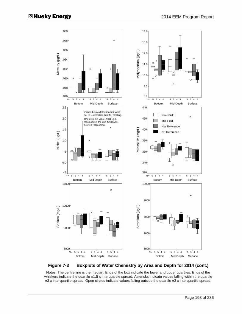
Submitted To 2014 EEM Program Report
Page 193 of 236
444 444 555 555N =
SurfaceMid-DepthBottom
Merc
ury
(µg/L
)
.030
.028
.026
.024
.022
.020
.018
.016444 444 555 555N =
SurfaceMid-DepthBottom
Mo
lyb
den
um
(µg
/L)
14.0
13.0
12.0
11.0
10.0
9.0
8.0
444 444 555 555N =
SurfaceMid-DepthBottom
Sodiu
m (
mg/L
)
11000
10000
9000
8000444 444 555 555N =
SurfaceMid-DepthBottom
Str
ontium
(µg/L
)
10000
9000
8000
7000
6000
444 444 555 555N =
SurfaceMid-DepthBottom
Pota
ssiu
m (
mg
/L)
440
420
400
380
360
340
320444 444 545 555N =
SurfaceMid-DepthBottom
Nic
kel (µ
g/L
)
2.5
2.0
1.5
1.0
.5
0.0
-.5
Values below detection limit were
set to ½ detection limit for plotting.
One extreme value (9.34 µg/L
measured in the mid-f ield) was
deleted for plotting.
Near-Field
Mid-Field
NW Reference
NE Reference
Figure 7-3 Boxplots of Water Chemistry by Area and Depth for 2014 (cont.)
Notes: The centre line is the median. Ends of the box indicate the lower and upper quartiles. Ends of the whiskers indicate the quartile ±1.5 x interquartile spread. Asterisks indicate values falling within the quartile ±3 x interquartile spread. Open circles indicate values falling outside the quartile ±3 x interquartile spread.

Submitted To 2014 EEM Program Report
Page 194 of 236
444 444 555 555N =
SurfaceMid-DepthBottom
Sulp
hur
(mg/L
)
1200
1100
1000
900
800444 444 555 555N =
SurfaceMid-DepthBottom
Ura
niu
m (
µg/L
)
4.4
4.2
4.0
3.8
3.6
3.4
3.2
3.0
2.8
2.6
444 444 555 555N =
SurfaceMid-DepthBottom
To
tal S
uspe
nd
ed
So
lids (
mg/L
)
2.0
1.5
1.0
.5
0.0444 444 555 555N =
SurfaceMid-DepthBottom
Un
ion
ize
d A
mm
on
ia (
mg
/L)
.005
.004
.003
.002
.001
0.000
Values below detection limit were
set to ½ detection limit for plotting.
Near-Field
Mid-Field
NW Reference
NE Reference
Figure 7-3 Boxplots of Water Chemistry by Area and Depth for 2014 (cont.)
Notes: The centre line is the median. Ends of the box indicate the lower and upper quartiles. Ends of the whiskers indicate the quartile ±1.5 x interquartile spread. Asterisks indicate values falling within the quartile ±3 x interquartile spread. Open circles indicate values falling outside the quartile ±3 x interquartile spread.

Submitted To 2014 EEM Program Report
Page 195 of 236
Table 7-3 Results of ANOVA (p-values) Testing Differences Between Areas and Depth
Variable p-values
Area Depth AxD
Arsenic 0.729 0.147 0.634
Barium 0.003** <0.001*** <0.001***
Boron 0.859 0.081 0.368
Calcium 0.067 0.006** 0.392
Lithium 0.448 0.007** 0.608
Magnesium 0.901 0.188 0.657
Mercury 0.154 0.937 0.756
Molybdenum 0.113 0.073 0.22
Nickel 0.788 0.631 0.451
Potassium 0.922 0.094 0.411
Sodium 0.36 0.344 0.711
Strontium 0.929 0.095 0.369
Sulphur 0.794 0.399 0.466
Uranium 0.386 0.173 0.503
TSS 0.101 0.618 0.711
Unionized Ammonia 0.140 <0.001*** 0.406
Notes: - ‘Area’ tests for differences among the four areas, overall. - ‘Depth' tests for depth differences, overall.
‘‘AxD' tests for differences in depth gradients among Areas. - Reported p-values for Area and Depth were from models with the interaction term removed
when the interaction term was not significant. - *p ≤ 0.05; **p ≤ 0.01; ***p ≤ 0.001 (in bold).
- High values for magnesium, potassium, strontium and sulphur were noted in one surface sample in the mid-field (see Figure 7-3 and Appendix D-2). Area differences remained non- significant (p > 0.05) for these variables with that one sample (W-7MF-SUR) removed.
With the exception of barium, no significant differences were noted between Areas (Table 7-3). Barium concentrations were higher at mid-depth in Reference Area samples, and barium concentrations were higher in near-field surface samples (Figure 7-3, Table 7-4). Differences were small. Median barium concentration in mid-depth Reference Area samples was 7.0 µg/L versus medians of 5.6 and 5.3 µg/L in the mid-depth near- and mid-field Study Area samples, respectively. Median barium concentration in near-field surface samples was 5.6 µg/L versus medians of 5.0 and 5.2 µg/L in the mid-field and Reference Areas, respectively.
Table 7-4 ANOVA by Depth Class for Barium
Depth Class Area S vs R NF vs R MF vs R
Surface 0.001** 0.095 0.012* 0.956
Mid-depth <0.001*** <0.001*** <0.001*** <0.001***
Bottom 0.690 0.451 0.456 0.608
Notes - 'Area' tests for differences among the four Areas, overall. - 'S vs R' tests for differences between the two Study Area and the two Reference Areas. - ‘NF vs R’ tests for a difference between the near-field and the Reference Areas. - ‘MF vs R’ tests for a difference between the mid-field and the Reference Areas. - *p ≤ 0.05; **p ≤ 0.01; ***p ≤ 0.001 (in bold).
In 2010, molybdenum and sulphur concentrations differed significantly between the Study Area and the Reference Areas, with concentrations lower in the Study Area in that year (Husky Energy 2011). In 2012, barium differed significantly between the Study and Reference Areas, with concentrations higher in bottom samples in the near- and mid-field, and lower in mid-depth and surface samples in those two Areas compared to the Reference Areas (Husky Energy 2013).

Submitted To 2014 EEM Program Report
Page 196 of 236
Figure 7-4 plots median barium concentration in 2010, 2012 and 2014 in the Study Area (2010)18, the combined Study Areas (2012 and 2014) and the combined Reference Areas (2010, 2012 and 2014). This figure indicates that median barium concentration have generally varied from approximately 3 to 9 µg/L. Differences among Areas were
greatest in 2012 and 2014, at mid-depth, with concentrations higher in the combined Reference Areas19.
0 2 4 6 8 10
Study Area
Reference Area
Study Area
Reference Area
Study Area
Reference Area
Bo
tto
mM
id-D
epth
Surf
ace
Barium (µg/L)
2014
2012
2010
Figure 7-4 Barium Concentration in the Combined Study and Reference Areas in 2010 2012 and 2014
Produced Water Constituents
As noted above, low concentrations of benzene and toluene (4 and 2 µg/L, respectively) were detected in one near-field surface sample (W-5NE-SUR, Appendix D-2) and, given that this sample was collected down-current from the SeaRose FPSO, these constituents could have been issued from produced water. A relatively high concentration of barium for surface samples (7.2 µg/L, see Figure 7-3) was also noted in that sample. Finally, copper was only detected at station W-5NE, in a mid-depth sample (copper concentration in that sample was 0.55 µg/L). Combined, these results indicate that produced water may have been detected at station W-5NE.
As noted above, one surface sample from a mid-field station (W-7MF-SUR) had elevated levels of magnesium, potassium, strontium and sulphur (see Appendix D-2), although this did not affect overall Area differences. Nickel was also elevated in one mid-depth sample in the mid-field (W-8MF-MID), without any effect on overall Area differences. Of these constituents, only strontium could be expected to be elevated by produced water input (Table 7-5). Therefore, it is unlikely that elevated levels for some variables noted at stations W-7MF and W-8MF resulted from produced water. Similarly, thallium, a constituent expected to be enriched in produced water, was elevated in the
18 Only one Study Area, with stations located up to 1 km of the SeaRose FPSO, was sampled in 2010. Reference Areas remained unchanged from 2010 to 2012. 19 The significantly higher concentration of barium in the near-field versus the Reference Areas in 2014 is not apparent with both the near- and mid-field data combined.

Submitted To 2014 EEM Program Report
Page 197 of 236
surface sample at W-1NE. However, as this was the only produced water constituent that was elevated, the observed concentration may not have resulted from produced water discharge.
7.3 Sediment
7.3.1 Modelling Study
Full model results predicting the concentration of selected produced water constituents in sediments were provided as part of the 2012 EEM report (Husky Energy 2013).
7.3.1.1 Constituent Selection
Concentrations of produced water constituents from the SeaRose FPSO were compared to concentrations in marine sediments around White Rose to identify those constituents that could settle to sediments at sufficiently high concentrations to act as tracers. Based on this, accumulation of Ra-228 was modelled, with results applicable to other potential tracers in produced water (see Husky Energy 2013 for details).
7.3.1.2 Conclusions and Recommendations
The following conclusions were drawn from the modelling study:
Radium radionuclides are not expected to be effective tracers of produced water constituents in sediments20.
Close attention should be paid to any increase in iron concentrations in sediments, particularly to the south, since modelling showed that deposition of constituents likely would be greater to the south of the SeaRose FPSO.
7.3.2 Field Sampling
7.3.2.1 Sediment Sample Collection and Laboratory Processing
Sediment collection and laboratory processing are described in Section 5. In addition to the sediment stations sampled as part of the Sediment Quality component of the EEM program (i.e., Sediment Quality Triad stations), one sediment core was also collected for chemistry analysis at those stations sampled for water (Figure 7-1).
7.3.2.2 Data Analysis
Quantitative analysis of sediment data for the Water Quality portion of the White Rose EEM program focuses on iron concentration in sediments, as per recommendations in Section 7.3.1.2. Quantitative analyses on other sediment quality variables at Sediment Quality Triad stations are provided in Section 5.
20 Based on this, the collection and examination of sediment radionuclide data as a potential tracer for produced water was discontinued.
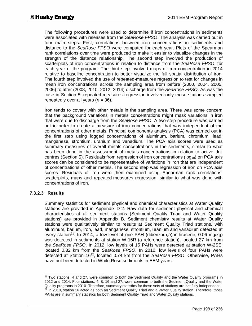
Submitted To 2014 EEM Program Report
Page 198 of 236
The following procedures were used to determine if iron concentrations in sediments were associated with releases from the SeaRose FPSO. The analysis was carried out in four main steps. First, correlations between iron concentrations in sediments and distance to the SeaRose FPSO were computed for each year. Plots of the Spearman rank correlations over time were produced to make it easier to visualize changes in the strength of the distance relationship. The second step involved the production of scatterplots of iron concentrations in relation to distance from the SeaRose FPSO, for each year of the program. The third step involved maps of iron concentration in 2014 relative to baseline concentration to better visualize the full spatial distribution of iron. The fourth step involved the use of repeated-measures regression to test for changes in mean iron concentrations across the sampling area from before (2000, 2004, 2005, 2006) to after (2008, 2010, 2012, 2014) discharge from the SeaRose FPSO. As was the case in Section 5, repeated-measures regression involved only those stations sampled repeatedly over all years (n = 36).
Iron tends to covary with other metals in the sampling area. There was some concern that the background variations in metals concentrations might mask variations in iron that were due to discharge from the SeaRose FPSO. A two-step procedure was carried out in order to create a measure of iron concentrations that was independent of the concentrations of other metals. Principal components analysis (PCA) was carried out in the first step using logged concentrations of aluminum, barium, chromium, lead, manganese, strontium, uranium and vanadium. The PCA axis scores were used as summary measures of overall metals concentrations in the sediments, similar to what has been done in the assessment of metals concentrations in relation to active drill centres (Section 5). Residuals from regression of iron concentrations (log10) on PCA axis scores can be considered to be representative of variations in iron that are independent of concentrations of other metals. The second step was regression of iron on PCA axis scores. Residuals of iron were then examined using Spearman rank correlations, scatterplots, maps and repeated-measures regression, similar to what was done with concentrations of iron.
7.3.2.3 Results
Summary statistics for sediment physical and chemical characteristics at Water Quality stations are provided in Appendix D-2. Raw data for sediment physical and chemical characteristics at all sediment stations (Sediment Quality Triad and Water Quality stations) are provided in Appendix B. Sediment chemistry results at Water Quality stations were qualitatively similar to results at Sediment Quality Triad stations, with aluminum, barium, iron, lead, manganese, strontium, uranium and vanadium detected at every station21. In 2014, a low-level of one PAH (dibenzo(a,h)anthracene; 0.06 mg/kg) was detected in sediments at station W-15R (a reference station), located 27 km from the SeaRose FPSO. In 2012, low levels of 15 PAHs were detected at station W-2SE, located 0.32 km from the SeaRose FPSO. In 2010, low levels of four PAHs were detected at Station 1622, located 0.74 km from the SeaRose FPSO. Otherwise, PAHs have not been detected in White Rose sediments in EEM years.
21 Two stations, 4 and 27, were common to both the Sediment Quality and the Water Quality programs in 2012 and 2014. Four stations, 4, 8, 16 and 27, were common to both the Sediment Quality and the Water Quality programs in 2010. Therefore, summary statistics for these sets of stations are not fully independent. 22 In 2010, station 16 acted as both an Sediment Quality Triad and a Water Quality station. Therefore, those PAHs are in summary statistics for both Sediment Quality Triad and Water Quality stations.

Submitted To 2014 EEM Program Report
Page 199 of 236
Principal Components Analysis
All metals were strongly associated (i.e., rP > |0.6|) with scores on the first PCA axis (Table 7-5); therefore, the first PCA axis was a good summary of overall concentrations of metals. Barium concentrations correlated strongly with both the first and second PCA axes; therefore, the second axis was a summary of variations in barium that were independent of variations in overall metals concentrations. Barium is examined in detail in Section 5. Residuals of iron concentrations (log10) were obtained from regression against scores on the first PCA axis.
Table 7-5 Principal Component Analysis Component Loadings (Correlations) of Metals Concentrations (All Years)
Parameter Principal Component
1 2
Aluminum 0.78 0.12
Barium 0.62 -0.68
Chromium 0.77 0.34
Lead 0.72 -0.58
Manganese 0.74 0.48
Strontium 0.86 -0.43
Uranium 0.69 0.23
Vanadium 0.78 0.43
Variance Explained 56 20
Note: - Bold indicates component loading (correlation) greater than 0.6 or -0.6.
Spearman Rank Correlations
Spearman rank correlations for iron in relation to distance to the SeaRose FPSO, and for iron residuals, for all years, are illustrated in Figures 7-5 and 7-6. Spearman rank
correlations were not significant for iron in 2014 (s = 0.06, p > 0.05, All stations; s = 0.15, p > 0.05, repeated-measures stations). Rank correlations were not significant for iron in any year (Figure 7-5).
Similarly ranked correlations were not significant for iron residuals when all stations or
repeated-measures stations were considered in 2014 (s = 0.14, p > 0.05, All stations;
s = 0.29, p > 0.05, repeated-measures stations; Figure 7-6).
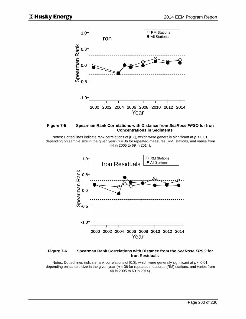
Submitted To 2014 EEM Program Report
Page 200 of 236
RM Stations
All StationsIron
2000 2002 2004 2006 2008 2010 2012 2014
Year
-1.0
-0.5
0.0
0.5
1.0
Spearm
an R
ank
2000 2002 2004 2006 2008 2010 2012 2014
-1.0
-0.5
0.0
0.5
1.0
Figure 7-5 Spearman Rank Correlations with Distance from SeaRose FPSO for Iron Concentrations in Sediments
Notes: Dotted lines indicate rank correlations of |0.3|, which were generally significant at p < 0.01, depending on sample size in the given year (n = 36 for repeated-measures (RM) stations, and varies from
44 in 2005 to 69 in 2014).
RM Stations
All StationsIron Residuals
2000 2002 2004 2006 2008 2010 2012 2014
Year
-1.0
-0.5
0.0
0.5
1.0
Spearm
an R
ank
2000 2002 2004 2006 2008 2010 2012 2014
-1.0
-0.5
0.0
0.5
1.0
Figure 7-6 Spearman Rank Correlations with Distance from the SeaRose FPSO for Iron Residuals
Notes: Dotted lines indicate rank correlations of |0.3|, which were generally significant at p < 0.01, depending on sample size in the given year (n = 36 for repeated measures (RM) stations, and varies from
44 in 2005 to 69 in 2014).

Submitted To 2014 EEM Program Report
Page 201 of 236
Scatterplots
The relationships between iron concentrations and iron residuals and distance to the SeaRose FPSO are illustrated in the Figures 7-7 and 7-8. The plots indicate no increase in iron concentrations in sediments near the SeaRose FPSO. The plots may indicate an increase in iron concentrations in 2008, 2010, 2012 and 2014 relative to the data from prior years (Figure 7-7), with this potentially more apparent for iron residuals between 2010 and 2014 (Figure 7-8).
Maps
Maps of stations with iron and iron residuals within and above the baseline background range are provided in Figures 7-9 and 7-10. Iron concentrations in Figure 7-9 are not corrected for the natural association between iron and other metals, and metals concentrations are elevated at the Northeast Reference Area. Those four stations are deeper than remaining stations and this could reflect a natural tendency for metals to increase with depth. The map of iron residuals (Figure 7-10), which would correct for the natural association among metals, does not show high iron at those four stations, relative to concentrations of other metals.
In 2012, there was a tendency for higher iron residuals between 5 and 10 km from the SeaRose FPSO, with more frequent enrichment to the south of the SeaRose FPSO (Husky Energy 2013). This increase in iron residuals between 5 and 10 km from the SeaRose FPSO was less apparent in 2014, but higher iron residual values did tend to occur more frequently to the northwest of the SeaRose FPSO.
Repeated-Measures Regression
Results of repeated-measures regression are provided in Table 7-6. For repeated-measures stations, there were no significant differences in slopes of the relations between iron or iron residuals and distance to the SeaRose FPSO from before to after produced water discharge began at the SeaRose FPSO in March, 2007. There has been a significant increase in sediment iron concentrations in the sampling area from before to after produced water discharge began at the SeaRose FPSO (p = 0.016), consistent with the scatterplots above. There was no change in mean iron residuals from before to after discharge began (p = 0.177).

Submitted To 2014 EEM Program Report
Page 202 of 236
0.1 1 10 100
FPSO D (km)
0
1000
2000
3000
4000
5000
Iron (
mg/k
g)
2000
0.1 1 10 100
FPSO D (km)
0
1000
2000
3000
4000
5000
Iron (
mg/k
g)
2004
0.1 1 10 100
FPSO D (km)
0
1000
2000
3000
4000
5000
Iron (
mg/k
g)
2005
0.1 1 10 100
FPSO D (km)
0
1000
2000
3000
4000
5000
Iron (
mg/k
g)
2006
0.1 1 10 100
FPSO D (km)
0
1000
2000
3000
4000
5000
Iron (
mg/k
g)
2008
0.1 1 10 100
FPSO D (km)
0
1000
2000
3000
4000
5000
Iron (
mg/k
g)
2010
0.1 1 10 100
FPSO D (km)
0
1000
2000
3000
4000
5000
Iron (
mg/k
g)
2012
0.1 1 10 100
FPSO D (km)
0
1000
2000
3000
4000
5000
Iron (
mg/k
g)
2014
Figure 7-7 Variation in Iron Concentrations in Sediments (mg/kg) with Distance from the SeaRose FPSO (all Years)
Notes: SeaRose FPSO D = distance (km) to the SeaRose FPSO. Background iron concentrations are indicated by horizontal lines (992 mg/kg and 1,970 mg/kg, respectively), based on the mean values ± 2 SDs
from 2000 (baseline).

Submitted To 2014 EEM Program Report
Page 203 of 236
0.1 1 10 100
FPSO D (km)
-0.30
-0.15
0.00
0.15
0.30
Iron R
esid
uals
2000
0.1 1 10 100
FPSO D (km)
-0.30
-0.15
0.00
0.15
0.30
Iron R
esid
uals
2004
0.1 1 10 100
FPSO D (km)
-0.30
-0.15
0.00
0.15
0.30
Iron R
esid
uals
2005
0.1 1 10 100
FPSO D (km)
-0.30
-0.15
0.00
0.15
0.30
Iron R
esid
uals
2006
0.1 1 10 100
FPSO D (km)
-0.30
-0.15
0.00
0.15
0.30
Iron R
esid
uals
2008
0.1 1 10 100
FPSO D (km)
-0.30
-0.15
0.00
0.15
0.30
Iron R
esid
uals
2010
0.1 1 10 100
FPSO D (km)
-0.30
-0.15
0.00
0.15
0.30
Iron R
esid
uals
2012
0.1 1 10 100
FPSO D (km)
-0.30
-0.15
0.00
0.15
0.30
Iron R
esid
uals
2014
Figure 7-8 Variation in Iron Residuals with Distance from the SeaRose FPSO (all Years)
Notes: SeaRose FPSO D = distance (km) to the SeaRose FPSO. Background iron residuals are indicated by horizontal lines (-0.113 and 0.047, respectively), based on the mean values ± 2 SDs from 2000
(baseline).

Submitted To 2014 EEM Program Report
Page 204 of 236
Figure 7-9 Location of Stations with Iron Concentrations Within and Outside the Baseline Range (2014)

Submitted To 2014 EEM Program Report
Page 205 of 236
Figure 7-10 Location of Stations with Iron Residuals Within and Outside the Baseline Range (2014)

Submitted To 2014 EEM Program Report
Page 206 of 236
Table 7-6 Repeated-measures Regression Testing for Changes in Iron Concentrations, and Iron Residuals over Time
Variable Change in Slope from Before to After Change in Mean from Before to After
Iron 0.119 0.016
Iron Residuals 0.174 0.177
Notes: - Values are probabilities. - n = 36
Variations in iron and iron residuals are illustrated in Figures 7-11 and 7-12. From these and analyses above, there is some evidence of enrichment of iron in sediments. Change, if any, in iron residuals since the release of produced water has been subtle.
2000 2002 2004 2006 2008 2010 2012 2014
Year
0
1000
2000
3000
4000
5000
Iro
n (
mg
/kg
)
Figure 7-11 Dot Density Plot of Iron Concentrations in Sediments (mg/kg) by Year
Note: Background iron concentrations are indicated by horizontal lines (992 mg/kg and 1,970 mg/kg, respectively), based on the mean values ± 2 SDs using data from 2000.
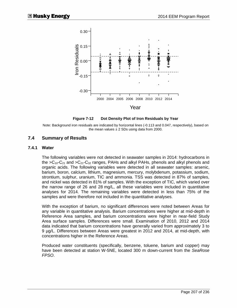
Submitted To 2014 EEM Program Report
Page 207 of 236
2000 2004 2005 2006 2008 2010 2012 2014
Year
-0.30
-0.15
0.00
0.15
0.30
Iro
n R
esid
ua
ls
Figure 7-12 Dot Density Plot of Iron Residuals by Year
Note: Background iron residuals are indicated by horizontal lines (-0.113 and 0.047, respectively), based on the mean values ± 2 SDs using data from 2000.
7.4 Summary of Results
7.4.1 Water
The following variables were not detected in seawater samples in 2014: hydrocarbons in the >C10-C21 and >C21-C32 ranges, PAHs and alkyl PAHs, phenols and alkyl phenols and organic acids. The following variables were detected in all seawater samples: arsenic, barium, boron, calcium, lithium, magnesium, mercury, molybdenum, potassium, sodium, strontium, sulphur, uranium, TIC and ammonia. TSS was detected in 87% of samples, and nickel was detected in 81% of samples. With the exception of TIC, which varied over the narrow range of 26 and 28 mg/L, all these variables were included in quantitative analyses for 2014. The remaining variables were detected in less than 75% of the samples and were therefore not included in the quantitative analyses.
With the exception of barium, no significant differences were noted between Areas for any variable in quantitative analysis. Barium concentrations were higher at mid-depth in Reference Area samples, and barium concentrations were higher in near-field Study Area surface samples. Differences were small. Examination of 2010, 2012 and 2014 data indicated that barium concentrations have generally varied from approximately 3 to 9 µg/L. Differences between Areas were greatest in 2012 and 2014, at mid-depth, with concentrations higher in the Reference Areas.
Produced water constituents (specifically, benzene, toluene, barium and copper) may have been detected at station W-5NE, located 300 m down-current from the SeaRose FPSO.

Submitted To 2014 EEM Program Report
Page 208 of 236
7.4.2 Sediment
Modelling results indicated that iron concentrations could potentially be enriched in sediments (Husky Energy 2013). In 2014, there was a tendency for iron enrichment to the northwest of the SeaRose FPSO, but this tendency was weaker than it was in 2012. As was the case in 2012, there was also some indication of an increase in iron since produced water discharge began at the SeaRose FPSO. At present, the link between iron enrichment in sediments and produced water release from the SeaRose FPSO remains weak. Continued examination is warranted in order to better assess this metal as a potential tracer of produced water constituents in sediments.

Submitted To 2014 EEM Program Report
Page 209 of 236
8.0 Discussion
8.1 Sediment Quality Component
Examination of sediment quality is standard in many EEM programs (e.g., Hurley and Ellis (2004) and references therein; Bjørgesaeter and Gray (2008); Netto et al. (2009); Pozebon et al. (2009); Santos et al. (2009)). The White Rose EEM program examines potential project effects on sediment chemistry, sediment toxicity and benthic community structure. These three sets of measurements are collectively known as the Sediment Quality Triad (Chapman 1992). The assessment of effects at White Rose is based on the change in relationships between Sediment Quality Triad variables and distance from the development. Distance to the nearest drill centre is used to assess drilling effects at the whole-field level. Occurrence above or below the range of values observed during baseline sampling (2000) is used to assess effects from individual drill centres.
8.1.1 Physical and Chemical Characteristics
In 2014, concentrations of >C10-C21 hydrocarbons and barium were elevated around all active drill centres, as was also the case in previous EEM years. The estimated zone of influence for >C10-C21 hydrocarbons from threshold models23 in 2014 was greater than the estimated zone of influence in 2012 and 2010, though less than all years prior to 2010. A threshold distance (distance at which concentrations are reduced to low or background level) of 5.8 km was noted in 2014, which was greater than upper 95% confidence intervals noted for both 2010 and 2012; 4.4 and 4.8 km, respectively. Threshold distances ranging from 5.9 to 10.4 km were noted in years prior to 2010. For barium, the estimated threshold distance was 1 km; unchanged from 2012 and less than in previous years. Thresholds distances for barium in previous years ranged from 1.9 to 3.624 km.
The maximum >C10-C21 hydrocarbon concentration in 2014 was 120 mg/kg (at station S5, located 0.31 km from the Southern Drill Centre) and the maximum barium concentration was 1,400 mg/kg (at station 20, located 0.37 km from the Central Drill Centre). The maximum observed concentrations of both >C10-C21 hydrocarbon and barium in 2014 were reduced compared to those observed in every year of the EEM program since baseline. Elevated concentrations of hydrocarbons and barium are expected near drill centres at offshore oil developments. Examples of concentrations at White Rose and at other developments are provided in Table 8-1. Levels of hydrocarbons and barium at White Rose were within the ranges noted from other projects and are among the lowest values of any of the listed project examples (Table 8-1).
23 Threshold models estimate the distance at which concentrations are reduced to low or background levels using distance to the nearest drill centre as the input variable. Details are provided in Section 5. 24 In part, the variation in threshold distances is a function of tightness of the relationship between the
analyte concentration and distance from nearest drill centre; strong correlations de facto produce shorter thresholds, while noisier relationships will produce longer threshold distances.

Submitted To 2014 EEM Program Report
Page 210 of 236
Table 8-1 Total Petroleum Hydrocarbons and Barium with Distance from Source at White Rose and at Other Developments
Location Year of Study
Distance from Source (m)
TPH (mg/kg)
Barium (mg/kg)
White Rose
2014
300 to 750 <0.3 to 120 140 to 1,400
750 to 2,500 0.45 to 21 150 to 560
2,500 to 5,000 <0.3 to 17 160 to 790
2012
300 to 750 <0.3 to 527 110 to 4,000
750 to 2,500 0.86 to 21.10 140 to 450
2,500 to 5,000 <0.3 to 3.18 140 to 210
2010
300 to 750 9.9 to 819 250 to 2,700
750 to 2,500 0.5 to 11.40 160 to 480
2,500 to 5,000 0.4 to 1.40 160 to 200
2008
300 to 750 2.2 to 1,615 170 to 3,400
750 to 2,500 1.3 to 55.7 160 to 600
2,500 to 5,000 <0.3 to 4.2 160 to 210
2006
300 to 750 1.5 to 576 200 to 3,100
750 to 2,500 0.7 to 53.4 150 to 770
2,500 to 5,000 <3 140 to 250
2005
300 to 750 <3 to 261.7 210 to 810
750 to 2,500 <3 to 54.6 140 to 380
2,500 to 5,000 <3 150 to 220
2004
300 to 750 8.99 to 275.9 190 to 1,400
750 to 2,500 <3 to 22.2 120 to 470
2,500 to 5,000 <3 to 6.9 140 to 230
2000
300 to 750 <3 140 to 180
750 to 2,500 <3 140 to 210
2,500 to 5,000 <3 150 to 210
Grand Banks, Terra Nova
(Suncor Energy 1998, 2001, 2002, 2003, 2005, 2007, 2009, 2011, 2013)
2012
140 to 750 <3 to 310 140 to 4,900
750 to 2,500 <3 to 7.5 72 to 330
2,500 to 5,000 <3 82 to 200
2010
140 to 750 <3 to 767 130 to 4,200
750 to 2,500 <3 to 339 87 to 420
2,500 to 5,000 <3 69 to 160
2008
140 to 750 <3 to 343 130 to 7,200
750 to 2,500 <3 to 11 89 to 280
2,500 to 5,000 <3 78 to 210
2006
140 to 750 8 to 986 240 to 16,000
750 to 2,500 <3 to 30 110 to 340
2,500 to 5,000 <3 89 to 230
2004
140 to 750 8 to 6,580 140 to 2,100
750 to 2,500 3 to 72 100 to 340
2,500 to 5,000 <3 to 4 63 to 190
2002
140 to 750 <3 to 931 110 to 2,200
750 to 2,500 <3 to 49 84 to 330
2,500 to 5,000 <3 to 5 83 to 200
2001 750 to 2,500 <3 to 30 100 to 190
2,500 to 5,000 <3 to 8 87 to 180
2000 750 to 2,500 <3 to 14 92 to 210
2,500 to 5,000 <3 to 6 80 to 230
1997 750 to 2,500 <3 87 to 190
2,500 to 5,000 <3 79 to 280
Gulf of Mexico (NPO-895) (Candler et al. 1995)
1993 50
200 2,000
134,428 80 to 11,460
24
47,437 542 to 5,641
Gulf of Mexico (MAI-686)
(Kennicutt et al. 1996) 1993
200 500
3,000
40 43 49
1,625 1,134 1,072

Submitted To 2014 EEM Program Report
Page 211 of 236
Location Year of Study
Distance from Source (m)
TPH (mg/kg)
Barium (mg/kg)
Gulf of Mexico (MU-A85) (Kennicutt et al. 1996)
1993 200 500
3,000
42.3 31.7 27.1
3,706 1,817 1,094
Gulf of Mexico (HI-A389) (Kennicutt et al. 1996)
1993 200 500
3,000
65 33 32
13,756 3,993 1,293
North Sea (Beatrice) (Addy et al. 1984)
1982 250 750
3,000
8 to 759 5 to 105 3 to 73
-
Dutch Continental Shelf (K14-13) (Daan and Mulder
1996) 200 54 to 161 -
North Sea
(Daan et al. 1994) 1994 200 2 to 4,700
Norway (Valhall)
(Hartley 1996) 1985
250 500
3,000 -
19,000 to 96,000 3,700 to 9,300
280 to 430
North Sea (Brent) (Massie et al. 1985)
1981 800
3,200 41 to 61 33 to 43
-
North Sea (Forties) (Massie et al. 1985)
1980 800
3,200 9 to 78
16 to 55 -
Gulf of Mexico (Matagorda 622) (Chapman et al. 1991; Brooks et al. 1990)
1987
25 150 750
3,000
757 ±1,818 6,233 12,333
980
Santa Maria Basin (Hidalgo) (Phillips et al. 1998)
1991 125 500
1,000 -
1,250 975
1,050
Norway (Ekofisk)
(Ellis and Schneider 1997) 1996
750 2,000 5,000
- 3,650 2,214 667
Norway (Gyda 2/1-9)
(Bakke et al. 1995) 1994 100 to 200 236 -
Norway (Tordis) (Gjøs et al. 1991)
1990 500 8,920 -
Norway (U/a 2/7-29) (Vik et al. 1996)
200 1,000 to 2,368 -
North Sea (UK)
(UKOOA 2001) 1975 to
1995
0 to 500 >500 to 2,000
>2,000 to 5,000
124 to 11,983 3 to 164 3 to 76
84 to 2,040 7 to 1595 8 to 729
Note: - TPH (total petroleum hydrocarbon) includes C6-C32 hydrocarbons. This range is reported for comparison to other offshore operations.
- Absolute barium levels should not be compared across projects because of potential differences in measurement techniques (Hartley 1996) and differences in background levels.
- Distance for White Rose in 2014 is distance to nearest of the Northern, Central, Southern, North Amethyst and South White Rose Extension Drill Centres. Distance for White Rose in 2010 and 2012 is distance to nearest of the Northern, Central, Southern and North Amethyst Drill Centres. Distance in 2000, 2005, 2006 and 2008 is distance to nearest of the Northern, Central and Southern Drill Centres. Distance in 2004 is distance to the nearest of the Northern and Southern Drill Centres.
- Station 31 at White Rose, near an exploration well drilled in 2007, was excluded from 2008, 2010, 2012 and 2014 statistics.
In 2014, project effects on sediment lead concentrations were noted. Those effects have also been noted since 2006, and threshold distances for lead have consistently decreased from a maximum 1.5 km in 2006 to a minimum 0.6 km in 2014, unchanged from 2012. In contrast to 2012 results, no significant project effects were found for strontium in 2014. There was no indication of project effects on sediment for other

Submitted To 2014 EEM Program Report
Page 212 of 236
metals and no sediment quality guidelines exceeded ISQGs (CCME 2001, 2015) (see Section 5).
In 2014, lead levels were higher near active drill centres, ranging from approximately 2.4 to 6.7 mg/kg as compared to 1.6 to 6.2 mg/kg at more distant stations. These lead levels were below the ISQG of 30.2 mg/kg., The maximum concentration for lead occurred at station S5, (0.31 km from the Southern Drill Centre) which was the station with the highest reported >C10-C21 hydrocarbon concentration.
For the first time, project effects on sediment fines concentrations were noted in 2014. A threshold distance of 0.7 km from the nearest active drill centre was estimated. As per lead and >C10-C21 hydrocarbons, the maximum percent fines value of 2.16% was observed at station S5, 0.31 km from the Southern Drill Centre. With the addition of 2014 data, mean percent fines values since operations began (1.21%) were significantly greater than the mean percent fines value of 1.03% recorded during baseline (2000) sampling.
Project effects on both TOC and ammonia were observed for the first time in 2014. The two greatest TOC concentrations in 2014 (8.4 and 7.2 g/kg) were observed at stations S3 (1.4 km from the nearest active drill centre) and S1 (0.6 km from the nearest active drill centre), respectively. TOC values from these two stations are the highest recorded concentrations since the beginning of the White Rose EEM program, representing 8.4-fold and 7.2-fold increases, respectively. That being said, the three next highest TOC concentrations (range = 2.8 to 5.4 g/kg) were recorded from stations 9, 10, and 22, with distances to the nearest active drill centre ranging from 1.61 to 7.89 km. As such, while 2014 TOC values did significantly decrease with distance from the nearest active drill centre, the absolute magnitude of TOC values across all stations in 2014 was greater than those observed in previous years. TOC ranged from <0.2 to 8.4 g/kg in 2014. In previous years, TOC values were limited to a range of approximately 0.4 to 2 g/kg (Appendix B-3 and Figure 5-24). Differences in the acid used to extract inorganic carbon between 2014 and previous years (o-phosphoric acid in 2014 versus hydrochloric acid in previous years) could explain the observed difference in results. Hydrochloric acid will dissolve some organic compounds, resulting in underestimation of TOC in samples having these compounds (J. Kiceniuk, pers. comm., 2015). Although this provides an explanation for the high values noted in 2014, it does not provide an explanation for the low values. Measurement error could also explain the wider spread (high and low values) noted in 2014.
In 2016, to be consistent and allow comparison to all previous EEM years except 2014, TOC will be measured at an accredited analytical laboratory and inorganic carbon will be extracted with hydrochloric acid.
With respect to ammonia, values significantly decrease with distance from the nearest active drill centre. All ammonia concentrations in 2014 were below the 12.2 mg/kg threshold established using stations with greater than 10 km from the nearest active drill centre since sampling for this analyte began in 2004 (n = 54). The two highest ammonia concentrations in 2014 (4.4 g/kg each) were observed at stations C2 (0.7 km from the nearest active drill centre) and 22 (7.9 km from the nearest active drill centre), respectively. Therefore, while ammonia showed a significantly declining trend with distance from the nearest active drill centre, it is important to note that this specific
Submitted To 2014 EEM Program Report
Page 213 of 236
indicator of organic matter decomposition was below background thresholds at all stations in 2014.
Project effects were also identified for both sulphide and redox potential. No threshold distance could be reliably estimated for these analytes; however, values did significantly vary with distance from the nearest active drill centre. As noted for TOC, the absolute magnitude of sulphide values across all stations in 2014 was greater than those observed in previous years. The five highest sulphide values in 2014 ranged from 1.53 to 5.1 mg/kg, with the greatest value recorded at station 20 (located 0.37 km from the Central Drill Centre), as was the case for barium. Station 20 has also had four of the ten highest sulphide values (8.7 to 21.6 mg/kg) recorded from any station since 2004. For redox potential, the only value below baseline concentrations was recorded at station S5; however, the observed value of 194 mV was well within the range of oxic conditions.
Sulphur levels increased significantly at some stations less than 1 km from active drill centres, with levels ranging from approximately 0.02% to 0.18% in the immediate vicinity of drill centres. No reliable threshold distance for effects could be estimated from the 2014 data. Sulphur is also a constituent of barite (BaSO4), and minor increases in sediment sulphur concentrations near active drill centres have been noted in previous years. Maximum sulphur levels occurred at two stations in 2014: C5 (0.18%), located 0.33 km from the Central Drill Centre; and NA1 (0.16%), located 0.29 km from the North Amethyst Drill Centre.
8.1.2 Laboratory Toxicity Tests
Sediments from certain stations were found to cause toxicity in the laboratory in 2014, though no direct effects related to project activity were readily apparent from the data. Toxicity testing focused on effects to bacterial luminescence and amphipod survival.
In 2014, three samples caused a significant decrease in bacterial luminescence at stations 19, N1 and N2. Station 19 is a reference station and is located 22 km from the nearest drill centre while stations N1 and N2 are located 2.2 and 1.5 km from the Northern Drill Centre, respectively. Only N1 and N2 exceeded baseline reference values for any key parameters. Each displayed elevated >C10-C21 hydrocarbons (0.45 mg/kg and 0.74 mg/kg, respectively relative to baseline values of 0.15 mg/kg) and reduced total biomass (263 g/m² and 349 g/m², respectively relative to baseline values of 367 g/m²). Previously, only one sample (in 2010) was classified as causing an effect to bacterial luminescence.
For amphipod survival, two samples in 2014 had more than 20% reduced survival and were significantly different from the reference station WRRS: station C1, located 1.1 km from the Central Drill Centre (64% survival); and station 16 (76% survival) located 5.59 km from the North Amethyst Drill Centre. Of these samples, station 16 had amphipod abundances below the lower benchmark of 44 per m². In 2012, one sample, from station N3 (0.6 km from the Northern Drill Centre), caused reduced survival to laboratory amphipods while sediments from the station nearest the Northern Drill Centre (station N4 at 0.3 km) were not toxic. Overall, amphipod survival in toxicity tests in most White Rose samples has been high (i.e., non-toxic) since operations began.

Submitted To 2014 EEM Program Report
Page 214 of 236
Percent amphipod survival in 2014 was not significantly correlated with any assessed variables. Further, no samples caused toxicity to both bacterial luminescence and amphipod survival.
8.1.3 Benthic Invertebrate Community Structure
Similar to 2012, analysis of benthic invertebrate community data from 2014 indicated there was weak evidence of project effects on total benthic species abundances, stronger evidence of effects on total biomass and little evidence of effects on richness. For individual taxa, there was strong evidence of project effects on Paraonidae (a family of polychaete worms) and minor yet statistically significant evidence of project effects on Spionidae (a family of deposit-feeding polychaetes), Tellinidae (a family of bivalve molluscs) and Amphipoda (a family of crustaceans).
Total benthic abundances, benthic biomass and numbers of Paraonidae were related to concentrations of >C10-C32 hydrocarbons and barium, as well as distance to the nearest active drill centre. Total abundances and biomass, and abundances of Paraonidae were lower in sediments with high concentrations of barium and >C10-C21 hydrocarbons. As was found in 2012, higher concentrations of sulphur and strontium in sediments also co-occurred with lower biomass and lower abundances of Paraonidae. In addition, Paraonidae abundance was negatively correlated with concentrations of lead and strontium while being positively correlated with redox potential. Interestingly, 2014 richness was positively correlated with concentrations of >C10-C32 hydrocarbons, barium, lead and strontium. Similar trends were noted between amphipod abundance and concentrations of >C10-C32 hydrocarbons and sulphur. The abundances of Spionidae polychaetes and Tellinidae were not significantly correlated with any sediment physical or chemical characteristics.
The assessment of the zone of effects on benthic invertebrates relied on: 1) an examination of changes in benthic indices, or taxa abundances, with distance from the nearest active drill centre (i.e., threshold models as described in Section 8.1.1); and 2) an examination of changes in benthic indices near individual drill centres (i.e., maps of indices or taxon abundance within or below the baseline range). The first approach can be regarded as a whole-field approach, whereas the second approach targets the effect of individual drill centres. This combined approach allows for the efficient assessment of effects of individual drill centres as well as potential cumulative effects from multiple drill centres.
The relationship between total benthic abundance and distance to the nearest active drill centre was relatively weak with abundance significantly greater with increasing distance from the nearest drill centre; no threshold distance for effects was established. Total abundance ranged from 1,050 to 5,920 organisms/m² near active drill centres (i.e., drill centre stations). The range for abundance at the most distant stations (more than 10 km from drill centres) was 2,230 to 6,215 organisms/m². Total abundance was lowest near the Central Drill Centre (mean = 2,465 organisms/m²); however, many stations farther away from drill centres, including the most distant stations, also had similarly low abundance, potentially reflecting natural variability.
Total biomass generally increased with distance from drill centres, varying from 4 to 1,193 g/m² near active drill centres to 232 to 1,643 g/m² at the most distant stations (more than 10 km from drill centres). The relationship between total biomass and

Submitted To 2014 EEM Program Report
Page 215 of 236
distance from the nearest active drill centre was significant in 2014, with a threshold distance for effects of approximately 5.5 km (95% confidence intervals: 1.5 to 20.1 km). This approximately 4-fold difference between the estimated threshold and the lower and upper confidence limits, not previously observed, appears to be driven by the variability in the relationship between biomass and distance to the nearest active drill centre. Many more samples closest to the drill centres and at intermediate distances (1 to 5 km) fell below background values in 2014 than in previous years. All drill centres, excepting SWRX, had more than one sample with relatively low total biomass (values ≤75% of baseline values) at distances ranging from 0.29 to 2.18 km from the nearest drill centre. Of these samples, most were found nearest to the North Amethyst and Southern Drill Centres. Additional analyses indicated that reductions in total biomass were associated with reductions in the numbers of larger echinoderms near active drill centres since sampling began in 2000. In contrast, echinoderm density has increased at Reference Stations 4, 12, 19 and 27 since sampling began in 2000.
Number of families per station (i.e., richness) varied between 22 and 56 in 2014, which is similar to the baseline range of between 21 and 38 families per station. As noted above, richness was positively correlated with concentrations of >C10-C32 hydrocarbons, barium, lead and strontium, though it was not correlated with distance from the nearest active drill centre. Richness values at all stations, including those nearest drill centres, were within the baseline range. From these data, there is insufficient evidence to conclude that richness was affected by project activity.
Responses of selected individual taxa at White Rose were examined to provide additional insight into the more general indices of community composition. Of the taxa examined, Paraonidae were clearly affected by project activities, but there was little evidence of project effects on Tellinidae and no evidence of project effects on Spionidae or Amphipoda.
As in previous years, Paraonidae abundance was strongly related to distance from the nearest active drill centre in 2014. Threshold distances for effects have been variable (1.5 km in 2014 to 4.1 km in 2004). Paraonidae abundances were reduced within: approximately 1.8 km from the Central Drill Centre; approximately 0.9 km from the Southern and North Amethyst Drill Centres; and approximately 2.2 km from the Northern Drill Centre. All of these distances are within the estimated range of threshold distances for the whole-field (0.5 to 3.0 km). Map results for the North Amethyst and the Northern Drill Centres indicate that effects on Paraonidae extended to between approximately 0.9 and 2.2 km, respectively.
As noted above, abundance of Spionidae, Tellinidae and Amphipoda were not significantly negatively related to any sediment physical and chemical characteristics. Abundances of these taxa were also unrelated to distance to the nearest active drill centre in 2014. Given these results, there is insufficient evidence to conclude that these taxa were affected by project activity.
8.1.4 Sediment Quality Summary
In summary, there were project effects on some sediment chemical characteristics and indices of benthic community at White Rose. Sediment concentrations of >C10-C21 hydrocarbons, barium, fines and lead were affected by project activity, with threshold distances estimated to range from 0.6 km for lead to 5.8 km for >C10-C21 hydrocarbons.

Submitted To 2014 EEM Program Report
Page 216 of 236
Project effects were also noted for TOC, ammonia, sulphide, sulphur and redox, which all varied significantly with proximity to drill centres in 2014, but threshold distances could not be estimated.
In terms of laboratory toxicity testing, all but three samples were non-toxic to bacterial bioluminescence, and all but two samples were non-toxic to amphipod survival. There was no association with toxicity of samples and distance from active drilling centres. No sample was assessed as toxic to both bacterial luminescence and amphipod survival. Amphipod survival in 2014 was not significantly correlated with any assessed variable.
Evidence of effects on total abundance, noted since 2005, was again marginal, with only a few stations affected and no threshold distance for effects. Benthic biomass was affected by project activity, with a threshold distance for effects of approximately 5.5 km (range: 1.5 to 20.1 km), seemingly related to an increase in the number of samples closest to the drill centres and at intermediate distances (1 to 5 km) with lower total biomass combined with decreases in the number of echinoderms near active drill centres. In general, echinoderms are not abundant around White Rose, but they are large organisms that account for a substantial proportion of benthic biomass.
As in previous years, no effects on richness were noted. The taxon most substantially affected by drilling activity, in term of numbers, remains the polychaete family Paraonidae. General increases or decreases noted for other Sediment Quality Triad components across the entire sampling area cannot reasonably be attributed to White Rose in the absence of relationships with distance from active drill centres, although these responses are of general interest.
After monitoring the effects of drilling on sediment quality seven times over a period of 11 years, distance relationships have varied somewhat in their strength, while threshold distances have also varied somewhat from year to year, with the annual variations depending on the analyte or measure of benthic community composition. With the exception of total biomass, there have been no trends to indicate that effects are getting greater in magnitude or in extent. This suggests that effects are staying the same from year to year, or potentially getting more localized.
8.2 Commercial Fish Component
8.2.1 Body Burden
On the East Coast of Canada, in the Gulf of Mexico, in the North Sea and elsewhere, fish and shellfish tissue have been examined for chemistry (body burden) to assess potential effects of offshore oil development on commercial fisheries resources (e.g., Rushing et al. 1991; Neff et al. 2000; Husky Energy 2004 and references therein; Armsworthy et al. 2005; DeBlois et al. 2005). At White Rose, American plaice liver and fillet and snow crab claw tissues from the Study Area and the four distant Reference Areas, (located 28 km from the centre of the White Rose development), are examined for body burden.
In 2014, most frequently detected compounds in plaice liver (arsenic, copper, iron, manganese, selenium, strontium, >C10-C21) did not vary significantly in concentration between the Study and Reference Areas. However, percent fat and concentrations of >C21-C32 hydrocarbons were significantly lower in the Study Area and percent moisture
Submitted To 2014 EEM Program Report
Page 217 of 236
and concentrations of cadmium and zinc were significantly higher in the Study Area. Compounds in the >C10-C21 and >C21-C32 hydrocarbon range were again detected in all liver samples in 2014. As in previous years, additional Gas Chromatography/Mass Spectrometry analysis did not indicate the presence of drill fluid or petroleum hydrocarbons in those samples, but a naturally occurring compound.
There were no significant differences between the Study Area and the Reference Areas in trends over time (2004 to 2014) for most frequently detected compounds in liver. However, a difference in linear trend over time between the Reference Areas and the Study Area was observed for percent moisture, with marginally higher concentrations in the Study Area across all years. There was also a significant difference in quadratic trends over time (increase followed by a decrease, or vice versa) between the Study and Reference Areas for >C21-C32 hydrocarbon concentrations, likely influenced by lower concentrations in the Reference Areas in 2006 and 2010.
There were no significant differences in percent fat, moisture, arsenic, iron, mercury, strontium and zinc content in plaice fillets between the Study Area and the Reference Areas in 2014. There were also no significant differences between the Study Area and the Reference Areas in trends over time (2004 to 2014), except for a significant difference in linear trends in zinc. Further examination of the data indicated that this difference was a statistical artefact, and the more appropriate quadratic function (given the area-wide decreases and subsequent increases in zinc) showed no difference between the Reference and Study Areas.
There were no significant differences between the Study Area and Reference Areas crab tissue in 2014 for frequently detected compounds (percent fat, percent moisture, arsenic, copper, iron, mercury, selenium, silver, strontium and zinc). Across years, significant differences in linear and/or quadratic trends between the Study and Reference Areas were noted for silver and mercury. Mercury concentrations remained relatively constant in the Study Area, while Reference Areas concentrations declined steeply from elevated levels in 2005. Silver has shown significant quadratic trends (initial values decreasing followed by an increase) at both the Study Area and Reference Areas (refer to Figure 6-11). However, Study Area concentrations of silver have generally remained within the range of variability of Reference Area concentrations.
Given the absence of differences between the Study and Reference Areas, many of the metals frequently detected in plaice and crab should be regarded as essential elements rather than contaminants originating from White Rose project activity (or any other anthropogenic source). Hydrocarbons have rarely been detected in edible tissue (crab claws and plaice fillets) at White Rose. Compounds in the >C10-C21 and >C21-C32 range frequently detected in plaice liver present as natural compounds, and not as a petrogenic source.
8.2.2 Taste Tests
There was no significant difference in taste between the Study and Reference Areas for both plaice and crab and there were no consistent comments from the taste panels identifying abnormal or foreign odour or taste. Results do not indicate the presence of taint in either resource.

Submitted To 2014 EEM Program Report
Page 218 of 236
8.2.3 Fish Health Indicators
Cellular and sub-cellular bioindicator responses along with observations of visible lesions on skin and internal organs are valuable monitoring tools for identifying adverse health conditions in animals in advance of population level responses. As such, they can provide early warning of potential health effects and aid in identifying their nature, scope and cause (see reviews by Payne et al. 1987; Peakall 1992; Society of Environmental Toxicology and Chemistry Special Publication Series 1992; Adams 2002; Tillitt and Papoulias 2003; Schlenk et al. 2008).
8.2.3.1 Biological Characteristics and Condition of Fish
Information on fish biological characteristics (morphometrics and life history characteristics) and condition is valuable for interpreting results of bioindicator studies (Levine et al. 1995; Barton et al. 2002). Therefore, fish biological characteristics were examined within the context of these studies.
Only one male fish was collected. With respect to maturity stages of female, there were significant differences in prevalence of pre-spawning and spent females between the Study Area and the combined Reference Areas, with a higher number of pre-spawning and spent females in the combined Reference Areas than in the Study Area.
Significant differences were found among References Areas for length, gutted weight and age as well as in liver weight versus gutted weight of pre-spawning females. When comparing the Study Area versus the combined Reference Areas, significant differences were found in age, gonad weight versus gutted weight and on liver weight versus gutted weight. In all cases, values from the combined Reference Areas were lower than in the Study Area. The difference in liver weight was attributed to fish from the Reference Area 2, which had lower liver weights than fish from all the other sites.
In the case of spent females, significant differences were observed among Reference Areas in gutted weight and gutted weight versus length. When comparing fish from the Study Area to those from the combined Reference Areas, significant differences were found only in gonad weight, with fish from the Study Area having significantly larger gonads than fish from the combined Reference Areas.
No statistical analyses were conducted on immature females (F-500) or partially spent females (F-550) due to low numbers of fish in this stages.
Overall, the differences observed in biological characteristics of fish between the two Areas could be attributed to normal inter-site variability linked to non-pollutant factors such as feeding and/or reproductive status (e.g., Mayer et al. 1989; Maddock and Burton 1999; Barton et al. 2002; Morgan 2003). For example, the way energy reserves such as liver glycogen are used by the fish as well as feeding behaviour and food availability may have a direct effect in the size of the liver (Barton et al. 2002).
8.2.3.2 Gross Pathology
Gross pathology was assessed visually in all fish during the necropsies for any external or internal abnormalities. There were no visible lesions on the skin or fins or on internal organs of any fish.

Submitted To 2014 EEM Program Report
Page 219 of 236
8.2.3.3 Haematology
Blood smears collected during the 2014 survey displayed signs of clotting, water micro-droplets and lack of uniformity, thus they were considered not suitable for carrying out reliable differential cell counts. Preliminary screening of the smears indicated that counts could vary by >20% upon examination of different regions of a slide. In human haematology, when 200 cells are counted, the variability is normally in the ± 7% to 10% range (Lynch et al. 1969). Oceans Ltd. considered the quality of smears too poor and the variability too high in the 2014 fish for carrying out haematological analysis.
During the environmental effects monitoring offshore surveys, including the 2014 survey, Oceans Ltd. has been tasked with collecting blood from American plaice to perform differential blood cell counts. This involves the preparation of blood smears at sea. However, the blood smears for the 2014 survey were not suitable for use in differential blood cell counts due to the following factors:
1. Samples showed various amounts of clotting. This has been an ongoing problem during different EEM surveys. To solve this problem the syringes were coated with EDTA prior to blood collection; however, this seemed to have no effect as various degrees of clotting were observed in the blood smears. It is worth mentioning that the blood collection tubes where the blood is stored for slide preparation, also contain EDTA as anticoagulant.
2. Microscopic droplets of water on the slides. Due to high humidity in the boat, microscopic droplets of water formed in the slides. These droplets affect the proper staining of the slides as well as the blood smear itself. Unfortunately, this was unavoidable due to environmental conditions aboard the vessel.
3. Blood smears have to be performed while the ship was either fishing or travelling to another sampling location. In several of the slides, there were indications of movement. That is, gaps in the continuity of the blood smear that indicate the blood spreader was lifted from the slide due most likely to the movement of the ship.
8.2.3.4 Mixed Function Oxygenase Activity
Since basal levels of MFO enzymes can vary seasonally between males and females of the same species (e.g., Walton et al. 1983; Mathieu et al. 1991), results were analyzed separately for each sex. Within the females, data were analyzed separately for immature, pre-spawning and spent females, since maturity stage can result in some loss of sensitivity for resolving contaminant mediated differences during spawning (e.g., Whyte et al. 2000).
No significant differences were found in hepatic EROD activity among Reference Areas in pre-spawning and spent females. However, when comparing fish from the Study Area and the combined Reference Areas, a significant lower hepatic EROD activity was observed in both pre-spawning and spent females from the combined Study Area.
In general, an induction (i.e., increase) of EROD activity is associated with chemical exposure (Andersson and Forlin 1992; Whyte et al. 2000; van der Oost et al. 2003). However, there are a number of chemical compounds that can cause an inhibition of

Submitted To 2014 EEM Program Report
Page 220 of 236
EROD activity or a decrease in basal activity of this enzyme in fish (Whyte et al. 2000). For example, 4-nonylphenol, benzene, and different pesticides have been shown to decrease EROD activity in fish (Arinç and Şen 1993; Arukwe et al. 1997; Whyte et al. 2000). It is possible that the lower EROD activity observed in the present study in fish from the Study Area might be due to increased levels of 17-β estradiol in the plasma of American plaice, since the fish were captured during their reproductive season. The lack of statistical significance in other markers of exposure (e.g., liver and gill lesions) during this study seems to add weight to this possibility.
8.2.3.5 Histopathology
Detailed studies were carried out on liver tissues of plaice with a focus on various lesions that have been associated with chemical toxicity in field and laboratory studies (e.g., Myers et al. 1987; Hinton et al. 1992; Johnson et al. 1993; Myers and Fournie 2002; ICES 2004; Blazer et al. 2007; Codi King et al. 2011).
No cases of nuclear pleomorphism, megalocytic hepatosis, focus of cellular alteration, fibrillar inclusions or inflammatory response were detected in any of the fish. Five cases of hepatocellular vacuolation likely due to gonadal maturation (Timashova 1981; Bodammer and Murchelano 1990; Couillard et al. 1997) were detected in two fish from the Study Area and in one fish from each of Reference Areas 1, 2 and 4.
Proliferation of macrophage aggregates was detected in 86 fish, 35 from the Study Area and in 7, 13, 16 and 15 fish from Reference Areas 1, 2, 3 and 4 respectively; however, no significant differences were found between fish from the Study and combined Reference Areas. The presence of parasites, most likely from the class myxosporean, was detected in the liver tissue of some fish but no significant differences in the prevalence of fish affected were found between the Study and combined Reference Areas. Although these liver conditions are of interest in relation to providing general information on their presence in the survey area, they are generally of lesser importance and not the result of the presence of chemical pollutants. However, it is important to note from an EEM perspective that liver lesions more commonly associated with chemical toxicity were absent.
As in the case of liver histopathology, no significant differences were found for any of the studied conditions in fish from the Study Area compared to the combined Reference Areas.
8.2.4 Commercial Fish Summary
Overall, results of the fish health survey carried out in 2014 indicated that the health of American plaice is similar between the Study Area and the Reference Areas.
8.3 Water Quality Component
The Water Quality monitoring program at White Rose currently involves collection of sediment and seawater samples around the SeaRose FPSO and in two Reference Areas, located approximately 28 km to the northeast and northwest of the SeaRose FPSO. These samples are assessed for water and sediment chemistry.

Submitted To 2014 EEM Program Report
Page 221 of 236
Based on results of modelling conducted in 2012 (see Husky 2013):
Near-field Study Area stations, located at approximately 300 m from the SeaRose FPSO, are positioned at the time of sampling so that they are down-current from the SeaRose FPSO.
Mid-field Study Area stations are located at 4 km from the SeaRose FPSO in the direction of the prevailing seasonal current (to the southeast of the SeaRose FPSO).
8.3.1 Seawater Chemistry
The following variables were not detected in seawater samples in 2014: hydrocarbons in the >C10-C21 and >C21-C32 ranges, PAHs and alkyl PAHs, phenols and alkyl phenols and organic acids. The following variables were detected in all seawater samples: arsenic, barium, boron, calcium, lithium, magnesium, mercury, molybdenum, potassium, sodium, strontium, sulphur, uranium, TIC and ammonia. TSS was detected in 87% of samples, and nickel was detected in 81% of samples. With the exception of TIC, which varied over the narrow range of 26 and 28 mg/L, all these variables were included in quantitative analyses for 2014. The remaining variables were detected in less than 75% of the samples and were therefore not included in the quantitative analyses.
With the exception of barium, no significant differences were noted between Study and Reference areas for any variable in quantitative analysis in 2014. Barium concentrations were higher at mid-depth in Reference Area samples and at surface in near-field Study Area samples. Differences were small. Examination of 2010, 2012 and 2014 data indicated that barium concentrations have generally varied from approximately 3 to 9 µg/L. Differences between Areas were greatest in 2012 and 2014, at mid-depth, with concentrations higher in the Reference Areas.
Because barium is a major constituent of drilling muds and it is enriched in produced water (see Appendix D-4), differences in barium concentrations noted among Areas in 2014 could partly be related to project activity. Jerez Vegueria et al. (2002) found no evidence of barium contamination in seawater samples near the Barcia de Campos oil field in Brazil. Similarly, no differences among Areas in barium levels were noted at White Rose in the 2010 EEM program.
Area differences in median barium concentration were not as great in 2014 as in 2012. Surface concentrations of barium at the Study Area in 2014 were greater than those observed in 2012, though reduced relative to 2010 levels. The difference in barium concentration between the Study Areas and the Reference Areas at the surface in 2014 resulted from lower levels in the Northeast Reference Area; differences were not distinguishable between the Northwest Reference Area and Study Area in 2014. Beyond this, Neff (2002) reports barium levels of approximately 15 µg/L in oceanic waters.
Therefore, barium levels at White Rose are within the background range25.
Produced water constituents (specifically, benzene, toluene, barium and copper) may have been detected at station W-5NE, located 300 m down-current from the SeaRose FPSO on the day of sampling.
25 Barium was not measured in water samples during baseline (2000). Therefore, only literature values are available.

Submitted To 2014 EEM Program Report
Page 222 of 236
8.3.2 Sediment Iron Concentration
Based on recommendations from the 2012 modelling exercise (see Husky 2013), sediment iron concentrations from 2000 to 2014 at both water quality and Sediment Quality Triad stations were examined.
Similar to 2012, qualitative examination of iron data (i.e., maps) from 2014 showed a tendency for iron enrichment at distances of approximately 5 to 10 km from the SeaRose FPSO. In contrast to 2012, where trends were noted to the south, in 2014 that tendency was greater to the north. Also as noted in 2012, data collected for 2014 indicated an increase in iron from before to after produced water discharge began at the SeaRose FPSO.
8.3.3 Water Quality Summary
With the exception of barium, no significant differences were noted in water quality between Areas for any variable in quantitative analysis in 2014. Overall, in 2014, barium concentration differences among Areas were small and the largest difference involved lower levels in the Study Areas compared to the Reference Areas at mid-depth.
At present, the link between iron enrichment in sediments and produced water release from the SeaRose FPSO is not strong, but examination of this metal as a potential as a tracer for produced water constituents in sediments should be continued.
8.4 Summary of Effects and Monitoring Hypotheses
As discussed in Section 1.7, monitoring hypotheses were developed in Husky Energy (2004) as part of EEM program design to test effects predictions and estimate physical and chemical zones of influence.
These hypotheses (reiterated in Table 8-2) were set up to guide interpretation of results. As noted in Section 1.7, the “null” hypothesis (H0) always state that no pattern will be observed.
Table 8-2 Monitoring Hypotheses
Sediment Component
H0: There will be no change in Sediment Quality Triad variables with distance or direction from project discharge sources over time.
Commercial Fish Component
H0(1): Project discharges will not result in taint of snow crab and American plaice resources sampled within the White Rose Study Area, as measured using taste panels.
H0(2): Project discharges will not result in adverse effects to fish health within the White Rose Study Area, as measured using histopathology, haematology and MFO induction.
Water Component
H0: The distribution of produced water from point of discharge, as assessed using moorings data and/or vessel-based data collection, will not differ from the predicted distribution of produced water.
Note: - No hypothesis was developed for plaice and snow crab body burden, as these tests are considered to be supporting tests, providing information to aid in the interpretation of results of other monitoring variables (taste tests and health).

Submitted To 2014 EEM Program Report
Page 223 of 236
Given results observed in the 2014 EEM program, the null hypothesis is rejected for the Sediment Component of the program, but null hypotheses are not rejected for the Commercial Fish and Water Components. Rejection of the null hypothesis for the Sediment Component was expected, since drill cuttings modelling and EIS predictions do indicate that there should be change in Sediment Quality Triad variables with distance from discharge sources. The following summarizes project effects and relates them to EIS predictions and/or literature-based information, as applicable.
As predicted, concentrations of >C10-C21 hydrocarbons and barium were elevated by drilling activity near drill centres. To a lesser extent, sediment lead, fines, TOC, ammonia, sulphide, sulphur, and redox potential were also affected by drilling. Elevated concentrations of >C10-C21 hydrocarbons and barium at White Rose in 2014 remain comparable to levels observed at other developments.
The spatial extent of contamination in 2014 was consistent with original predictions on the spatial extent of the zone of influence of drill cuttings (9 km from source; Hodgins and Hodgins 2000; Section 1.5). >C10-C21 hydrocarbon contamination extended to 5.8 km from source. Barium contamination extended to 1 km from source. Percent fines extended to 0.7 km and lead contamination extended to 0.6 km from source. The threshold distance model was not significant for TOC, ammonia, sulphide, sulphur and redox potential.
In 2014, three samples significantly reduced bacterial luminescence at stations 19, N1 and N2. Station 19 is a reference station and is located 22 km from the nearest drill centre. Stations N1 and N2 are located 2.2 and 1.5 km from the Northern Drill Centre, respectively. Two stations significantly reduced amphipod survival; station C1, located 1.1 km from the Central Drill Centre, had 64% survival, and station 16, located 5.59 km from the North Amethyst Drill Centre, had 76% survival. Taken together, the bacterial luminescence and amphipod toxicity tests indicate that there is no evidence of project-related effects to sediments in White Rose field.
In 2014, as in the last two EEM years, evidence of effects on total abundance was relatively weak, benthic biomass was affected by project activity and there was little evidence of project effects on richness. The taxon most affected by project activity remains Paraonidae. As in 2012, there was little evidence of project effects on Spionidae, Tellinidae and Amphipoda abundance.
The threshold distance model was not significant for total abundance, indicating that the relationship with distance was relatively weak. The threshold distance model for total biomass was significant in 2014, with effects noted to within approximately 5.5 km from source, an increase of 4.0 km relative to 2012. Effects on Paraonidae extended to approximately 1.5 km from source, a decrease of 1.0 km compared to 2012. As noted in 2012, an examination of the spatial extent of effects by drill centre in 2014 indicated that effects from the Central and Southern Drill Centres overlapped. For total biomass, effects around the North Amethyst Drill Centre, which was probably less affected by the proximity of another drill centre, extended to approximately 1.0 km from source.
As noted in previous EEM reports, the spatial extent of effects on benthic invertebrates at White Rose is generally consistent with the literature on effects of contamination from offshore oil developments. Davies et al. (1984) first described general zones of effects on benthic invertebrates around offshore platforms. The first zone was characterized by

Submitted To 2014 EEM Program Report
Page 224 of 236
a highly disrupted benthic community within approximately 0.5 km of discharge source. The second zone was described as a transition zone in benthic community structure from affected to unaffected. This scheme has been generally used elsewhere. For instance, Gerard et al. (1999) also describe a zone of approximately 0.5 km from source with a highly disrupted benthic community. Based on their review, the spatial extent of the transition zone from affected to unaffected could extend from 0.2 to 2 km.
The White Rose (Husky oil 2000) and North Amethyst (LGL 2006) environmental assessments predictions are consistent with observations of both Davies et al. (1984) and Gerard et al. (1999); highly disrupted communities can be expected near source. The environmental assessments estimated the spatial extent of effects around individual drill centres and predicted that effects on benthic communities would extend to approximately 0.5 km from any one drill centre. On a per-drill centre basis and because both literature results and results at White Rose can only be approximate, the EEM results for 2014 support EIS predictions, with effects noted from approximately 0.3 to 2.18 km from source.
Ratings of effects size are provided by Davies et al. (1984) and Kilgour et al. (2005). Davies et al. (1984) describes a highly disrupted community as impoverished and highly modified with abundances at or near zero. In agreement, Kilgour et al. (2005) state that benthic community effects are large when they co-occur with effects on fish and that this normally occurs when the benthic community is reduced to one or two types of organisms, and with either very high (10x more than normal) or very low (10x less than normal) abundances. This is not the condition at White Rose. In the worst case in 2014, total abundance was reduced to approximately 75% or less than the lower limit of the baseline range of variation at one station near active drill centres 26 . Biomass was reduced to 75% or less of the lower limit of the baseline range at 11 stations near active drill centres, more than the four stations in 2012 yet comparable to the nine stations noted in 2010. Richness levels did not fall to less than 75% of the baseline range at any drill centre station in 2014, as in previous years. Overall, richness has remained within the range of values noted in the baseline year (2000).
In spite of changes in sediment contamination and benthic invertebrate responses since drilling began at White Rose in 2004, there has generally not been any consistent accentuation of contamination or responses over those years. While total biomass appears to be more affected relative to previous years, this is likely being driven by echinoderm abundance as observed in previous years.
Zones of influence of project contaminants and effects on benthic community indices and taxa have not increased in severity or extent over time. As there has been no continued and consistent degradation at White Rose, sediment contamination and the benthic invertebrate responses justify continued monitoring without further mitigation.
Sediment contamination and effects on benthos noted in 2014 and in previous years have not translated into effects on the fisheries resources, as indicated by fish health assessment and taint tests. No project-related tissue contamination was noted for crab and plaice, neither resource was tainted, and plaice health was similar between White
26 See Section 5 for a list of stations and distances near drill centres where values were reduced to below 75% of the baseline range.

Submitted To 2014 EEM Program Report
Page 225 of 236
Rose and more distant Reference Areas. These results indicate that changes in sediments and benthic community have not translated to effects to commercial fish.
There was no evidence of project effects on water quality.
8.5 Recommendations for the 2014 EEM program
8.5.1 Sediment Quality
Based upon the results of the 2014 WR EEM program, the following recommendations are proposed to increase the efficiency, rigour, and defensibility of the sediment quality component:
1. If retained, repeated-measures regression should be modified to include categorical predictor variables (a.k.a., “dummy variables”) that explicitly test the effect of active drill centres, both individually and cumulatively. Paraonidae abundances, for example, have shown the potential to be influenced by the combined effects of multiple drill centres as recently as 2012. Such a modification to the statistical analyses would permit a more robust examination of the data and assessment of potential cumulative effects. Alternatively, in the absence of statistical differences, these tests would provide greater certainty in any conclusions that project-related effects do not exist.
2. Future assessment of the benthic community at White Rose should focus on a more holistic and rigourous approach to data analysis procedures and interpretation. The current program examines three summary indices (total abundance, total biomass, and taxonomic richness), and abundances of key taxonomic groups (Paraonidae, Spionidae, Tellinidae, Amphipoda, and Echinodermata) in isolation with basic multivariate ordination (Principal Components Analyses) to attempt to understand biotic relationships with sediment physical and chemical characteristics.
Newer multivariate techniques are available that are more useful in assessing biological-physical-chemical relationships in fewer tests with more statistical rigour and defensibility. These newer techniques are currently implemented as part of standard operational procedures in other international offshore oil and gas jurisdictions (International Association of Oil & Gas Producers 2012), such as Norway (Norwegian Climate and Pollution Agency 2011) and Italy (Manoukian et al. 2010)
8.5.2 Commercial Fish
In 2014, the retrieval speed of the trawl was adjusted so that the trawl was raised at the bottom at a slower speed. This resulted in lower mortality to bycatch. It is recommended that trawls continue to be retrieved at reduced speeds to allow for better survival of by-catch species, such as cod.
Due to the factors described in Section 8.2.3.3, and because the remaining health indices measured during the EEM program are sufficient to provide an overall assessment of fish health, we recommend that the haematological analysis be removed from the tasks to be performed during future offshore EEM surveys.

Submitted To 2014 EEM Program Report
Page 226 of 236
In accordance with a recommendation from Fisheries and Oceans Canada on the 2012 EEM report, histological staging of gonad development for plaice was performed and compared to the visual staging method used in prior EEM years. Results did not indicate that histological staging is a warranted replacement for visual staging (Appendix C-3, Annex E). Therefore, this method should not be used in future EEM years.
8.5.3 Water Quality
In 2014, there was some indication (albeit weak) that iron could act as a tracer of produced water constituents in sediments. Therefore, the analysis of iron in sediments using chemistry data from both Sediment Quality Triad and water quality stations should continue in 2016.
8.6 Regulator Comments on the 2012 EEM Program
Husky Energy actions and responses to comments from the regulatory community on the 2012 EEM report are provided in Appendix A.

Submitted To 2014 EEM Program Report
Page 227 of 236
9.0 References
9.1 Personal Communications
Kiceniuk, J., Environmental Scientist, Halifax, Nova Scotia.
Maxxam Analytics, Halifax, Nova Scotia.
petroforma inc., St. John’s, Newfoundland and Labrador.
Pocklington, P., Arenicola Marine Limited, Wolfville, Nova Scotia.
9.2 Literature Cited
Adams, S.M. (Editor). 2002. Biological Indicators of Aquatic Ecosystem Stress. American Fisheries Society, Bethesda, MD. 644 pp.
Addy, J.M., J.P. Hartley and P.J.C. Tibbetts. 1984. Ecological effects of low toxicity oil-based mud drilling in the Beatrice Oilfield. Mar. Poll. Bull., 15(12): 429-436.
Agius, C. 1979a. The role of melano-macrophage centres in iron storage in normal and diseased fish. J. Fish Dis., 2: 337-43.
Agius, C. 1979b. Aspects of the Melano-macrophage Centres in Fish. PhD Thesis, University of Stirling, Stirling, UK.
Agius, C. and R.J. Roberts. 1981. Effects of starvation on the melano-macrophage centers of fish. J. Fish Biol., 19: 161-9.
Andersson, T. and L. Forlin. 1992. Regulation of the cytochrome P450 enzyme system in fish. Aquat. Toxicol., 24: 1-19.
Armsworthy, S.L., P.J. Cranford, K. Lee and T. King. 2005. Chronic Effects of Synthetic Drilling Muds on Sea Scallops (Placopecten magellanicus). In: S.L. Armsworthy, P.J. Cranford and K. Lee (eds.). Offshore Oil and Gas Environmental Effects Monitoring: Approaches and Technologies, Battelle Press, Columbus, Ohio.
Arinç, E. and A. Şen. 1993. Effects of in vivo benzene treatment on cytochrome P450 and mixed-function oxidase activities of gilthead seabream (Sparus aurata) liver microsomes. Comp. Biochem. Physiol. C., 104: 61-65.
Arukwe, A., L. Förlin and A. Goksøyr. 1997. Xenobiotic and steroid biotransformation enzymes in Atlantic salmon (Salmo salar) liver treated with an estrogenic compound, 4-nonylphenol. Environ.Toxicol. Chem., 16: 2576-2583.
Bakke, T., J.S. Gray, R.G. Lichtenthaler and K.H. Palmork. 1995. Environmental Surveys in the Vicinity of Petroleum Installations on the Norwegian Shelf Report for 1993. SFT, Report No. 95: 15. SFT’s Expert Group for Evaluation of Offshore Environmental Surveys (in Norwegian with English summary).

Submitted To 2014 EEM Program Report
Page 228 of 236
Barton, B.A., J.D. Morgan and M.M. Vijayan. 2002. Physiological and condition-related indicators of environmental stress in fish. Pp. 111-148. In: M. Adams (ed.). Biological indicators of Aquatic Ecosystem Stress, Bethesda, MD.
Bjørgesaeter, A. and J.S. Gray. 2008. Setting Sediment Quality Guidelines: A simple yet effective method. Mar. Poll. Bull., 57: 221-235.
Blazer, V.S., Fournie, J.W., Wolf, J.C. and M.J. Wolfe. 2007. Manual for the Microscopic Diagnosis of Proliferative Liver and Skin Lesions in the Brown Bullhead (Ameiurus nebulosus). Pennsylvania Sea Grant. 38 pp.
Bodammer, J.E. and R.A. Murchelano. 1990. Cytological study of vacuolated cells and other aberrant hepatocytes in winter flounder from Boston Harbour. Canc. Res., 50: 6744-6756.
Botta, J.R. 1994. Sensory evaluation of tainted aquatic resources. Pp. 257-273. In: J.W. Kiceniuk and S. Ray (eds.). Analysis of Contaminants in Edible Aquatic Resources. VCH Publishers, New York, NY.
Brooks, J.M., M.C. Kennicutt, T.L. Wade, A.D. Hart, G.J. Denoux and T.J. McDonald. 1990. Hydrocarbon distributions around a shallow water multiwell platform. Env. Sci. Techn., 24: 1079-1085.
Brown C.L. and C.J. George. 1985. Age-dependent accumulation of macrophage aggregation in the yellow perch, Perca flavescens (Mitchill). J. Fish Dis., 8: 135-138.
Canada-Newfoundland Offshore Petroleum Board. 2001. Decision 2001.01: Application for Approval – White Rose Canada-Newfoundland Benefits Plan and White Rose Development Plan. St. John’s, NL.
Candler, J., E.S. Hoskin, M. Churan, C.W. Lai and M. Freeman. 1995. Seafloor Monitoring for Synthetic-Based Mud Discharge In the Western Gulf of Mexico. Paper presented at the SPE/USEPA Exploration and Production Environmental Conference held in Houston, TX, 27-29 March 1995.
CCME (Canadian Council of Ministers of the Environment). 2001. Canadian sediment quality guidelines for the protection of aquatic life: Summary Tables. Updated. In Canadian Environmental Quality Guidelines, 1999, Canadian Council of Ministers of the Environment, Winnipeg, MB.
CCME (Canadian Council of Ministers of the Environment). 2015. Water Quality Guidelines for the Protection of Aquatic Life. Available at: http://st-ts.ccme.ca/en/index.html?chems=all&chapters=all
Chapman, P.M. 1992. Pollution status of North Sea sediments: An international integrative study. Mar. Ecol. Prog. Ser., 91: 313-322.
Chapman, P.M., R.N. Dexter, H.A. Anderson and E.A. Power. 1991. Evaluation of effects associated with an oil platform, using the Sediment Quality Triad. Environ. Toxicol. Chem., 10: 407-424.

Submitted To 2014 EEM Program Report
Page 229 of 236
Chapman, P.M., R.N. Dexter and E.R. Long. 1987. Synoptic measures of sediment contamination, toxicity and infaunal community structure (the Sediment Quality Triad) in San Francisco Bay. Mar. Ecol. Prog. Ser., 37: 75-96.
Codi King, S., C. Conwell, M. Haasch, J. Mondon, J. Mueller, S. Zhu and L. Howitt. 2011. Field evaluation of a suite of biomarkers in an Australian tropical reef species, stripey seaperch (Lutjanus carponotatus): Assessment of produced water from the Harriet A Platform. Pp. 261-294. In: K. Lee and J. Neff (eds.). Produced Water Discharge from Offshore Oil and Gas Facilities: Environmental Risks and Advances in Mitigation Technologies, Springer Publishing Company, New York.
Couillard, C.M., P.V. Hodson and M. Castonguay. 1997. Correlations between pathological changes and chemical contamination in American eels, Anguilla rostrata, from the St. Lawrence River. Can. J. Fish. Aquat. Sci., 54: 1916-1927.
Daan, R. and M. Mulder. 1996. On the short-term and long-term impacts of drilling activities in the Dutch sector of the North Sea. ICES J. Mar. Sci., 53: 1036-1044.
Daan, R., M. Mulder and A.V. Leeuwen. 1994. Differential sensitivity of macrozoobenthic species to discharges of oil drill cuttings in the North Sea. Netherl. J. Sea Res., 33(1): 113-127.
Davies, J.M., J.M. Addy, R.A. Blackman, J.R. Blanchards, J.E. Ferbrache, D.C. Moore, H.J. Somerville, A. Whitehead and T. Wilkinson. 1984. Environmental effects of the use of oil-based drilling muds in the North Sea. Mar. Poll. Bull., 15, 363-370.
DeBlois, E.M., C. Leeder, K.C. Penney, M. Murdoch, M.D. Paine, F. Power and U.P. Williams. 2005. Terra Nova environmental effects monitoring program: From Environmental Impact Statement onward. Pp. 475-491. In: S.L. Armsworthy, P.J. Cranford and K. Lee (eds.). Offshore Oil and Gas Environmental Effects Monitoring: Approaches and Technologies, Battelle Press, Columbus, OH. 631 pp.
Ellis, A.E. 1976. Leucocytes and related cells in the plaice Pleuronectes platessa. J. Fish Biol., 8: 143-156.
Ellis, J.L. and D.C. Schneider. 1997. Evaluation of a gradient design for environmental impact assessment. Env. Monitor. Assess., 48: 157-172.
Environment Canada. 1992. Biological Test Method: Toxicity Test using Luminescent Bacteria Photobacterium phosphoreum. Report EPS 1/RM/24. Environment Canada, Environmental Protection Service, Ottawa, ON.
Environment Canada. 1998. Reference Method for Determining Acute Lethality of Sediment to Marine or Estuarine Amphipods. Report EPS 1/RM/35. Environment Canada Environmental Protection Service, Ottawa, ON.
Environment Canada. 2002. Biological Test Method: Reference Method for Determining the Toxicity of Sediment Using Luminescent Bacteria in a Solid-Phase Test. Report EPS 1/RM/42.

Submitted To 2014 EEM Program Report
Page 230 of 236
Gjøs, N., F. Oreld, T. Øfsti, J. Smith and S. May. 1991. ULA Well Site 7/12-9 Environmental Survey 1991. Report for BP Norway Ltd. 66 pp. + Appendices.
Goede R.W. and B.A. Barton. 1990. Organismic indices and an autopsy-based assessment as indicators of health and condition of fish. Pp. 93-108. In: S.M. Adams (ed.). Biological Indicators of Stress in Fish, American Fisheries Symposium 8, Bethesda, MD.
Green, R.H. 1979. Sampling Design and Statistical Methods for Environmental Biologists. John Wiley and Sons, Toronto, ON.
Hartley, J.P. 1996. Environmental monitoring of offshore oil and gas drilling discharges - a caution on the use of barium as a tracer. Mar. Poll. Bull., 32(10): 727-733.
Hinton, D.E., P.C. Baumann, G.R. Gardner, W.E. Hawkins, J.D. Hendricks, R.A. Murchelano and M.S. Okihiro. 1992. Histopathologic biomarkers. Pp. 155-209. In: R.J. Hugget, R.A. Kimerle, P.M. Mehrle, Jr. and H.L. Bergman (eds.). Biomarkers: Biochemical, Physiological and Histological Markers of Anthropogenic Stress, Lewis Publishers, Chelsea, MI.
Hodgins, D.O and S.L.M. Hodgins. 2000. Modeled predictions of Well Cuttings Deposition and Produced Water Dispersion for the Proposed White Rose Development. Part Two Document by Seaconsult Marine Research Ltd for Husky Oil Operations Ltd. 45 pp.
Hoke, R.A., J.P. Geisy and J.R. Adams. 1990. Use of linear orthogonal contrasts in environmental data. Environmental Toxicology and Chemistry, 9: 815-819.
Hurley, G. and J. Ellis. 2004. Environmental Effects of Exploratory Drilling Offshore Canada: Environmental Effects Monitoring Data and Literature Review - Final Report. Prepared for the Canadian Environmental Assessment Agency - Regulatory Advisory Committee. 114 pp.
Husky Energy. 2001. White Rose Baseline Characterization Report. Report prepared by Jacques Whitford Environment Limited for Husky Oil Operations, St. John’s, NL. 109 pp. + Appendices.
Husky Energy. 2003. White Rose Baseline Addendum. 2002 Biological Cruise. Report prepared by Jacques Whitford for Husky Energy, St. John’s, NL. 14 pp. + Appendices.
Husky Energy. 2004. White Rose Environmental Effects Monitoring Design Report. Report prepared by Jacques Whitford Environment Limited for Husky Oil Operations, St. John’s, NL. 42 pp. + Appendices
Husky Energy. 2005. White Rose Environmental Effects Monitoring Program. Prepared by Jacques Whitford Limited for Husky Energy, St. John’s, NL.
Husky Energy. 2006. White Rose Environmental Effects Monitoring Program. Prepared by Jacques Whitford Limited for Husky Energy, St. John’s, NL.

Submitted To 2014 EEM Program Report
Page 231 of 236
Husky Energy. 2007. White Rose Environmental Effects Monitoring Program. Prepared by Jacques Whitford Limited for Husky Energy, St. John’s, NL.
Husky Energy. 2008. White Rose Environmental Effects Monitoring Program Design Report 2008 (Revision). Report prepared by Elisabeth DeBlois Inc. for Husky Energy, St. John’s, NL.
Husky Energy. 2009. White Rose Environmental Effects Monitoring Program. Prepared
by Jacques Whitford Limited for Husky Energy, St. John’s, NL.
Husky Energy. 2010a. White Rose Water Quality Monitoring Program. Report No.:
WRHSE-RP-1584.
Husky Energy. 2010b. White Rose Environmental Effects Monitoring Design Report
(Revised 2010). Report No.: WR-HSE-RP-2008.
Husky Energy. 2011. White Rose Environmental Effects Monitoring Program. Prepared
by Stantec Consulting Ltd. for Husky Energy, St. John’s, NL.
Husky Energy. 2013. White Rose Environmental Effects Monitoring Program. Prepared
by Stantec Consulting Ltd. for Husky Energy, St. John’s, NL.
Husky Energy. 2014. White Rose Environmental Effects Monitoring Program Design Report 2014 (Revision). Report prepared by Elisabeth DeBlois Inc. for Husky Energy, St. John’s, NL.
Husky Oil Operations Limited. 2000. White Rose Oilfield Comprehensive Study. Part One: Environmental Impact Statement. Submitted to the Canada-Newfoundland Offshore Petroleum Board, St. John’s NL.
ICES (International Council for the Exploration of the Sea). 2004. Biological of contaminants: Use of liver pathology of the European flatfish dab (Limanda limanda) and flounder (Platichthys flesus) for monitoring. By S.W. Feist, T. Lang, G.D. Stentiford, and A. Kohler. ICES Techniques in Marine Environmental Sciences, No 38, 42p.
International Association of Oil & Gas Producers. 2012. Offshore Environmental Monitoring for the Oil & Gas Industry. OPG Report, No. 457. Available at: http://www.ogp.org.uk/
Jerez Vegueria, S.F., J.M. Godoy and N. Miekeley. 2002. Environmental impact studies of barium and radium discharges by produced waters from the “Bacia de Campos” oil-field offshore platforms, Brazil. Journal of Environmental Radioactivity, 62: 29-38.
Johnson, L.U., C.M. Stehr. O.P. Olson. M.S. Myers. S.M. Pierce. C.A. Wigren, B.B. McCain and U. Varanasi. 1993. Chemical contaminants and hepatic lesions in winter flounder (Pleuronectes americanus) from the Northeast Coast of the United States. Environ. Sci. Technol., 27(13): 2759-2771.
Kennicutt, M.C., R.H. Green, P. Montagna and P.F. Roscigno. 1996. Gulf of Mexico Offshore Operations Monitoring Experiment (GOOMEX), Phase I: Sublethal

Submitted To 2014 EEM Program Report
Page 232 of 236
responses to contaminant exposure – introduction and overview. Can. J. Fish. Aquat. Sci., 53: 2540-2553.
Kilgour, B.W., K.R. Munkittrick, C.B. Portt, K. Hedley, J. Culp, S. Dixit and G. Pastershank. 2005. Biological criteria for municipal wastewater effluent monitoring programs. Water Qual. Res. J. Can., 40: 374-387.
Larmond, E. 1977. Laboratory Methods for Sensory Evaluation of Food. Department of Agriculture. Research Branch, Ottawa, ON. 73 pp.
Levine, S.L., J.T. Oris and T.E. Wissing. 1995. Influence of environmental factors on the physiological condition and hepatic ethoxyresorufin O-deethylase (EROD) activity of gizzard shad (Dorosoma cepedianum). Environ. Toxicol. Chem., 14(1): 123-128.
LGL Limited. 2006. Husky White Rose Development Project: New Drill Centre Construction and Operations Program Environmental Assessment. LGL Report SA883, by LGL Limited, St. John’s, NL, for Husky Energy Inc., Calgary, AB. 299 pp. + Appendices.
Long, E.R. and P.M. Chapman. 1985. A Sediment Quality Triad: Measures of sediment contamination, toxicity and infaunal community composition in Puget Sound. Mar. Poll. Bull., 16: 405-415.
Lynch, M., S. Raphael, L. Mellor, P. Spare and M. Inwood. 1969. Medical Laboratory Technology and Clinical Pathology. Saunders (W.B.) Co. Limited, Philadelphia, PA. 1359 pp.
Maddock, D.M. and M.P. Burton. 1999. Gross and histological observations of ovarian development and related condition changes in American plaice. J. Fish Biol., 53: 928-944.
Manoukian S., A. Spagnolo, G. Scarcella, E. Punzo, R. Angelini and G. Fabi. 2010. Effects of two offshore gas platforms on soft-bottom benthic communities (northwestern Adriatic Sea, Italy). Mar. Environ. Res., 70: 402-410.
MARPOL (73/78). International Convention for the Prevention of Pollution from Ships, 1973, as modified by the Protocol of 1978 relating thereto. IMO Convention. http://www.imo.org/Conventions/contents.asp?doc_id=678&topic_id=258.
Massie, L.C., A.P. Ward, J.M. Davies and P.R. Mackie. 1985. The effects of oil exploration and production in the northern North Sea: Part 1 – The levels of hydrocarbons in water and sediments in selected areas, 1978-1981. Mar. Env. Res., 15: 165-213.
Mathieu, A., P. Lemaire, S. Carriere, P. Drai, J. Giudicelli and M. Lafaurie. 1991. Seasonal and sex linked variations in hepatic and extra hepatic biotransformation activities in striped mullet (Mullus barbatus). Ecotox. Environ. Safety, 22: 45-57.
Submitted To 2014 EEM Program Report
Page 233 of 236
Mayer, F.L., D.J. Versteeg, M. McKee, L.C. Folmar, R.L. Graney, D.D. McCume and B.A. Rattner. 1989. Physiological and nonspecific biomarkers. Pp. 5-85. In: R.J. Huggett, R.A. Kimerle, P.M. Mehrle, Jr. and H.L. Bergman (eds.). Biomarkers. Biochemical, Physiological, and Histological Markers of Anthropogenic Stress, Proceedings of the Eighth Pellston Workshop. Lewis Publishers, Keystone, CO. 347 pp.
Morgan, M.J. 2003. A preliminary examination of variability in condition of American plaice in NAFO divisions 3NLO. Northwest Atlantic Fisheries Organization (NAFO) SCR Doc., 03/11: 14 pp.
Myers, M.S. and J.W. Fournie. 2002. Histopathological biomarkers as integrators of anthropogenic and environmental stressors. Pp. 221-287. In: M. Adams (ed.). Biological Indicators of Aquatic Ecosystem Stress, American Fisheries Society, Bethesda, MD. 656 pp.
Myers, M.S., L.D. Rhodes and B.B. McCain. 1987. Pathologic anatomy and patterns of occurrence of hepatic neoplasms, putative preneoplastic pesions, and other idiopathic hepatic conditions in English sole (Parophrys vetulus) from Puget Sound, Washington. J. Nat., Cancer Inst., 78 (2): 333-363.
National Energy Board, Canada-Newfoundland and Labrador Offshore Petroleum Board and Canada-Nova Scotia Offshore Petroleum Board. 2010. Offshore Waste Treatment Guidelines. vi + 28 pp.
Neff, J.M. 2002. Bioaccumulation in Marine Organisms: Effect of Contaminants from Oil Well Produced Water. Elsevier Science Ltd., Oxford, UK. xv + 452 pp.
Neff, J.M., S. McKelvie and R.C. Ayers. 2000. Environmental Impacts of Synthetic Based Drilling Fluids. US Department of Interior Minerals Management Services, Gulf of Mexico OCS Region. Available at: http://www.gomr.mms.gov/PI/ PDFImages/ESPIS/3/3175.pdf
Netto, S.A., F. Gallucci and G. Fonseca. 2009. Deep-sea meiofauna response to synthetic-based drilling mud discharge off SE Brazil. Deep-Sea Res. II, 56: 41-49.
Norwegian Climate and Pollution Agency. 2011. Guidelines for Offshore Environmental Monitoring: The Petroleum Sector on the Norwegian Continental Shelf. Report No. TA 2849: 45 pp. + Appendices.
OSPAR (Oslo and Paris Commission). 1998. JAMP guidelines for contaminant-specific biological effects monitoring. OSPAR Agreement 2008-9. OSPAR, London, UK.
Payne, J.F., L. Fancey, A. Rahimtula and E. Porter. 1987. Review and perspective on the use of mixed-function oxygenase enzymes in biological monitoring. Comp. Pharmacol. Physiol., 86C(2): 233-245.
Peakall, D. 1992. Animal Biomarkers as Pollution Indicators. Chapman & Hall Ecotoxicology Series. 291 pp.
Submitted To 2014 EEM Program Report
Page 234 of 236
Phillips, C., J. Evans, W. Hom and J. Clayton. 1998. Long-term changes in sediment barium inventories associated with drilling-related discharges in the Santa Maria Basin, California, USA. Env. Tox. Chem., 17(9): 1653-1661.
Platt, WR. 1969. Color Atlas and Textbook or Hematology. Lippincott Company, Philadelphia, PA. 445 pp.
Pohl, E.L. and J.R. Fouts. 1980. A rapid method for assaying the metabolism of 7-Ethoxyresorufin by microsomal subcellular fractions. Analyt. Biochem., 107: 150-155.
Porter, E.L., J.F. Payne, J. Kiceniuk, L. Fancey and W. Melvin. 1989. Assessment of the potential for mixed-function oxygenase enzyme introduction in the extrahepatic tissues of cunners during reproduction. Mar. Env. Res., 28: 117-121.
Pozebon, D., J.H.Z. Santos, M.C.R. Peralda, S.M. Maia, S. Barrionuevo and T.M. Pizzolato. 2009. Metals, arsenic and hydrocarbon monitoring in marine sediment during drilling activity using NAFs. Deep-Sea Res. II, 56: 22-31.
Roberts, R.J. 1989. Melanin-containing cells of teleost fish and their relation to disease. Pp. 399-428. In: W.E. Ribelin and G. Migaki (eds.). The Pathology of Fishes, University of Wisconsin Press, Madison, WI.
Rushing, J.H., M.A. Churan and F.V. Jones. 1991. Bioaccumulation from Mineral Oil-wet and Synthetic Liquid-wet Cuttings in an Estuarine Fish, Fundulus grandis. SPE Health, Safety and Environment in Oil and Gas Exploration and Production Conference, 11-14 November 1991, The Hague, Netherlands.
Santos, M.F.L, P.C. Lana, J. Silva, J.G. Fachel and F.H. Pulgati. 2009. Effects of non-aqueous fluids cuttings discharge from exploratory drilling activities on the deep-sea macrobenthic communities. Deep-Sea Res. II, 56: 32-40.
Schlenk, D., R. Handy, S. Steinert, M.H. Depledge and W. Benson. 2008. Biomarkers. Pp. 683-733. In: R.T. Di Giulio and D.E. Hinton (eds.). The Toxicology of Fishes, CRC Press.
Society of Environmental Toxicology and Chemistry Special Publication Series. 1992. Biomarkers: Biochemical, Physiological, and Histological Markers of Anthropogenic Stress. R.J. Huggett, R.A. Kimerle, P.M. Mehrle, Jr. and H.L. Bergman (eds.). Technical Workshop held in Keystone, Colorado, July 23-28, 1989. Proceedings published in a SETAC Special Publication by Lewis Publishers, MI.
Suncor Energy. 1998. Terra Nova Baseline Characterization Data Report. Prepared by Jacques Whitford Environment Limited for Petro-Canada, St. John’s, NL. 17 pp. + Appendices.
Suncor Energy. 2001. 2000 Terra Nova Environmental Effects Monitoring Program. Prepared by Jacques Whitford Environment Limited for Petro-Canada, St. John’s, NL. 147 pp. + Appendices.

Submitted To 2014 EEM Program Report
Page 235 of 236
Suncor Energy. 2002. 2001 Terra Nova Environmental Effects Monitoring Program. Prepared by Jacques Whitford Environment Limited for Petro-Canada, St. John’s, NL. 194 pp. + Appendices.
Suncor Energy. 2003. 2002 Terra Nova Environmental Effects Monitoring Program. Prepared by Jacques Whitford Environment Limited for Petro-Canada, St. John’s, NL. 235 pp. + Appendices.
Suncor Energy. 2005. 2004 Terra Nova Environmental Effects Monitoring Program. Prepared by Jacques Whitford Limited for Petro-Canada, St. John’s, NL.
Suncor Energy. 2007. 2006 Terra Nova Environmental Effects Monitoring Program. Prepared by Jacques Whitford Limited for Petro-Canada, St. John’s, NL.
Suncor Energy. 2009. 2008 Terra Nova Environmental Effects Monitoring Program. Prepared by Jacques Whitford Stantec Limited for Suncor Energy Inc., St. John’s, NL.
Suncor Energy. 2011. 2010 Terra Nova Environmental Effects Monitoring Program. Prepared by Stantec Consulting Ltd. for Suncor Energy Inc., St. John’s, NL.
Suncor Energy. 2013. 2012 Terra Nova Environmental Effects Monitoring Program. Prepared by Stantec Consulting Ltd. for Suncor Energy Inc., St. John’s, NL.
Tay, K. L., K. G. Doe, A. J. MacDonald and K. Lee. 1998. The influence of particle size ammonia and sulfide on toxicity of dredged materials for ocean disposal. Pp. 559-574. In: P.G. Wells, K. Lee and C. Blaise (eds.). Microscale Testing in Aquatic Toxicology - Advances, Techniques and Practice, CRC Lewis Publishers, FL.
Tillitt, D.E. and D.M. Papoulias. 2003. Closing the gap between exposure and effects in monitoring studies. Pure Appl. Chem., 75(11-12): 2467-2475.
Timashova, L.V. 1981. Seasonal changes in the structure of the liver of the plaice, Pleuronectes platessa. J. Ichthyol., 21: 145-151.
UKOOA (United Kingdom Offshore Operators Association). 2001. An Analysis of UK Offshore Oil & Gas Environmental Surveys 1975-95. A study carried out by Heriot-University at the request of The United Kingdom Offshore Operators Association. 141 pp. + Appendices. Available at: http://www.ukooa.co.uk/issues/ ukbenthos/environsurvey.htm.
Underwood, A.J. 1993. The mechanics of spatially replicated sampling programmes to detect environmental impacts in a variable world. Aust. J. Ecol., 18: 99-116
van der Oost, R., J. Beyer and N.P.E. Vermeulen. 2003. Fish bioaccumulation and biomarkers in environmental risk assessment: a review. Environ. Toxicol. Pharmacol., 13: 57-149.
Submitted To 2014 EEM Program Report
Page 236 of 236
Vik, E.A., S. Dempsey and B.S. Nesgård. 1996. Evaluation of Available Test Results from Environmental Studies of Synthetic Based Drilling Muds. Report Prepared for Norwegian Oil Industry Association (OLF), Report No. 96-010: 127 pp.
Walton, D.G., L.L. Fancey, J.M. Green, J.W. Kiceniuk and W.R. Penrose. 1983. Seasonal changes in aryl hydrocarbon hydroxylase activity of a marine fish Tautogolabrus adspersus (walbaum) with and without petroleum exposure. Comp. Biochem. Physiol., 76C: 247-253.
Whyte, J.J., R.E. Jung, C.J. Schmitt and D.E. Tillitt. 2000. Ethoxyresorufin-O-deethylase (EROD) activity in fish as a biomarker of chemical exposure. Critical Rev. Toxicol., 30(4): 347-570.