report - pub.tik.ee.ethz.ch · 1 abstract a analysis method for embedded systems, called real time...

Institut fürTechnische Informatik undKommunikationsnetze

Valerio Bürker & Roman Hiestand

ReportTool für die Bewertung von Eingebetteten Systemen

Design und Integration einer Analysemethode in SymTA/S

Student Thesis SA-2004-2128th April 2004 / Summer Term 2004

Tutor: Simon KünzliSupervisor: Prof. Lothar Thiele

1

Abstract

A analysis method for embedded systems, called Real Time Calculus (RTC), has been devel-oped at the institute TIK of ETH Zurich in the last years. The method has not been embeddedin a graphical tool so far and therefore TIK has been looking for a possible implementation.A tool, called SymTA/S, to analyze embedded systems based on certain known analysismethods has been developed at TU Braunschweig. This tool fulfills the requirement of the TIKmethods and therefore the idea was to integrate the TIK method into SymTA/S.

This semester thesis shows how this implementation has been done. It starts with anevaluation of the requirements for the tool and gives then a detailed explanation about thechosen generic way of integrating the TIK method into this existing tool.

The major part of this thesis explains the exact implementation and the concepts behindit and further some details about the calculation flow.

Finally, it provides a short user guide which describes the usage of the TIK analysismethod specific parts of the SymTA/S tool. Furthermore, it shows an analysis example.

CONTENTS 2

Contents

1 Introduction 51.1 Problem Description . . . . . . . . . . . . . . . . . . . . . . . . . . . . . . . . . . 5

1.1.1 Subject . . . . . . . . . . . . . . . . . . . . . . . . . . . . . . . . . . . . . 51.1.2 Semester Thesis Task . . . . . . . . . . . . . . . . . . . . . . . . . . . . . 5

1.2 Approach . . . . . . . . . . . . . . . . . . . . . . . . . . . . . . . . . . . . . . . . 51.2.1 Understanding Analysis Methods . . . . . . . . . . . . . . . . . . . . . . . 51.2.2 Define Specifications . . . . . . . . . . . . . . . . . . . . . . . . . . . . . . 51.2.3 Get to Know SymTA/S . . . . . . . . . . . . . . . . . . . . . . . . . . . . . 51.2.4 Implementation . . . . . . . . . . . . . . . . . . . . . . . . . . . . . . . . . 51.2.5 Documentation . . . . . . . . . . . . . . . . . . . . . . . . . . . . . . . . . 5

1.3 Related Work . . . . . . . . . . . . . . . . . . . . . . . . . . . . . . . . . . . . . . 61.3.1 Analysis Method from TIK . . . . . . . . . . . . . . . . . . . . . . . . . . . 61.3.2 SymTA/S . . . . . . . . . . . . . . . . . . . . . . . . . . . . . . . . . . . . 6

2 Tool Specifications 72.1 Drawing Curves . . . . . . . . . . . . . . . . . . . . . . . . . . . . . . . . . . . . . 7

2.1.1 Functionality . . . . . . . . . . . . . . . . . . . . . . . . . . . . . . . . . . 72.1.2 Coordinate Plan . . . . . . . . . . . . . . . . . . . . . . . . . . . . . . . . 72.1.3 Upper and Lower Curve . . . . . . . . . . . . . . . . . . . . . . . . . . . . 7

2.2 Import and Export Format . . . . . . . . . . . . . . . . . . . . . . . . . . . . . . . 72.3 Data Structure . . . . . . . . . . . . . . . . . . . . . . . . . . . . . . . . . . . . . 8

2.3.1 Source Task . . . . . . . . . . . . . . . . . . . . . . . . . . . . . . . . . . 82.3.2 Regular Task . . . . . . . . . . . . . . . . . . . . . . . . . . . . . . . . . . 82.3.3 Sink Task . . . . . . . . . . . . . . . . . . . . . . . . . . . . . . . . . . . . 8

2.4 Curve Types . . . . . . . . . . . . . . . . . . . . . . . . . . . . . . . . . . . . . . 82.4.1 Alpha Curve . . . . . . . . . . . . . . . . . . . . . . . . . . . . . . . . . . 92.4.2 Alpha Prime Curve . . . . . . . . . . . . . . . . . . . . . . . . . . . . . . . 92.4.3 Beta Curve . . . . . . . . . . . . . . . . . . . . . . . . . . . . . . . . . . . 92.4.4 Beta Prime Curve . . . . . . . . . . . . . . . . . . . . . . . . . . . . . . . 9

2.5 Resources . . . . . . . . . . . . . . . . . . . . . . . . . . . . . . . . . . . . . . . 92.5.1 Scheduling Policies . . . . . . . . . . . . . . . . . . . . . . . . . . . . . . 9

2.6 Execute Analysis . . . . . . . . . . . . . . . . . . . . . . . . . . . . . . . . . . . . 10

3 SymTA/S 11

4 The Idea of Generic Objects and Libraries 134.1 General Structure . . . . . . . . . . . . . . . . . . . . . . . . . . . . . . . . . . . 134.2 Libpreferences.xml . . . . . . . . . . . . . . . . . . . . . . . . . . . . . . . . . . . 134.3 SymTA/S Core . . . . . . . . . . . . . . . . . . . . . . . . . . . . . . . . . . . . . 144.4 Data structure . . . . . . . . . . . . . . . . . . . . . . . . . . . . . . . . . . . . . . 14

4.4.1 Generic Resource . . . . . . . . . . . . . . . . . . . . . . . . . . . . . . . 144.4.2 Generic Process . . . . . . . . . . . . . . . . . . . . . . . . . . . . . . . . 144.4.3 Further Generic Data Structure Classes . . . . . . . . . . . . . . . . . . . 15

4.5 GUI . . . . . . . . . . . . . . . . . . . . . . . . . . . . . . . . . . . . . . . . . . . 154.6 Analysis . . . . . . . . . . . . . . . . . . . . . . . . . . . . . . . . . . . . . . . . . 15

5 Implementation 165.1 GUI . . . . . . . . . . . . . . . . . . . . . . . . . . . . . . . . . . . . . . . . . . . 16

5.1.1 Curve Drawer . . . . . . . . . . . . . . . . . . . . . . . . . . . . . . . . . . 165.1.2 Task and Resource Containers . . . . . . . . . . . . . . . . . . . . . . . . 18

5.2 Data Structure . . . . . . . . . . . . . . . . . . . . . . . . . . . . . . . . . . . . . 195.2.1 Class Curve . . . . . . . . . . . . . . . . . . . . . . . . . . . . . . . . . . 205.2.2 Class CurveSegment . . . . . . . . . . . . . . . . . . . . . . . . . . . . . 205.2.3 Class ProcessTIK . . . . . . . . . . . . . . . . . . . . . . . . . . . . . . 205.2.4 Class ResourceTIK . . . . . . . . . . . . . . . . . . . . . . . . . . . . . 215.2.5 Interface Drawable . . . . . . . . . . . . . . . . . . . . . . . . . . . . . . 22

5.3 Analysis . . . . . . . . . . . . . . . . . . . . . . . . . . . . . . . . . . . . . . . . . 23

CONTENTS 3

5.3.1 Calculation Flow . . . . . . . . . . . . . . . . . . . . . . . . . . . . . . . . 235.3.2 Class Analysis . . . . . . . . . . . . . . . . . . . . . . . . . . . . . . . . 245.3.3 Scheduler . . . . . . . . . . . . . . . . . . . . . . . . . . . . . . . . . . . . 265.3.4 FPS Scheduler . . . . . . . . . . . . . . . . . . . . . . . . . . . . . . . . . 275.3.5 TMDA Scheduler . . . . . . . . . . . . . . . . . . . . . . . . . . . . . . . . 285.3.6 Class WCET_calculation . . . . . . . . . . . . . . . . . . . . . . . . . . 295.3.7 Package Singlenode . . . . . . . . . . . . . . . . . . . . . . . . . . . . . 29

6 Short user manual 306.1 How To Use? . . . . . . . . . . . . . . . . . . . . . . . . . . . . . . . . . . . . . . 30

6.1.1 Tasks and Resources . . . . . . . . . . . . . . . . . . . . . . . . . . . . . 306.1.2 Curve Drawer . . . . . . . . . . . . . . . . . . . . . . . . . . . . . . . . . . 32

6.2 Analysis Example . . . . . . . . . . . . . . . . . . . . . . . . . . . . . . . . . . . 33

7 Outlook 36

8 Summary 37

A Acknowledgements 38

B Bibliography / References 39

C Example of a Curve XML File 40

D Libpreferences.xml 41

LIST OF FIGURES 4

List of Figures

1 Example for Fixed Priority Scheduling . . . . . . . . . . . . . . . . . . . . . . . . 82 Print Screen of SymTA/S Tool from TU Braunschweig, source: [11]. . . . . . . . . 113 Structure of Library Idea . . . . . . . . . . . . . . . . . . . . . . . . . . . . . . . . 134 UML Diagram for the Generic Resource . . . . . . . . . . . . . . . . . . . . . . . 155 UML Diagram for the Generic Process . . . . . . . . . . . . . . . . . . . . . . . . 156 Class Structure . . . . . . . . . . . . . . . . . . . . . . . . . . . . . . . . . . . . . 167 Coordinate Transformation . . . . . . . . . . . . . . . . . . . . . . . . . . . . . . . 178 Coordinate Rotation . . . . . . . . . . . . . . . . . . . . . . . . . . . . . . . . . . 189 Source Tasks and Appendant Curve Drawer Windows . . . . . . . . . . . . . . . 1910 UML Diagram of Data Structure . . . . . . . . . . . . . . . . . . . . . . . . . . . . 1911 Curve Segments of a Staircase Function . . . . . . . . . . . . . . . . . . . . . . . 2012 UML Diagram of Process Structure . . . . . . . . . . . . . . . . . . . . . . . . . . 2113 UML Diagram of Resource Structure . . . . . . . . . . . . . . . . . . . . . . . . . 2214 UML Diagram of Interface Drawable . . . . . . . . . . . . . . . . . . . . . . . . . 2215 Example to Explain the Calculation Flow Implemented in the Library . . . . . . . 2316 Architecture of the Method Analysis . . . . . . . . . . . . . . . . . . . . . . . . . 2417 Example of a Deadlock . . . . . . . . . . . . . . . . . . . . . . . . . . . . . . . . 2518 Architecture of the Error Handling . . . . . . . . . . . . . . . . . . . . . . . . . . . 2619 UML Diagram of the Environment of Scheduler Class . . . . . . . . . . . . . . . 2720 Weighted Beta Curves with the Option Evaluate Window Size and a Window Size

of 1.0 . . . . . . . . . . . . . . . . . . . . . . . . . . . . . . . . . . . . . . . . . . 2921 Weighted Beta Curves without the Option Evaluate Window Size . . . . . . . . . 2922 Properties of a Source Task . . . . . . . . . . . . . . . . . . . . . . . . . . . . . . 3023 Properties of a Regular Task . . . . . . . . . . . . . . . . . . . . . . . . . . . . . 3124 Properties of a Sink Task . . . . . . . . . . . . . . . . . . . . . . . . . . . . . . . 3125 Properties of a Resource . . . . . . . . . . . . . . . . . . . . . . . . . . . . . . . 3226 Curve Drawer Window . . . . . . . . . . . . . . . . . . . . . . . . . . . . . . . . . 3227 Simulation Example . . . . . . . . . . . . . . . . . . . . . . . . . . . . . . . . . . 3328 Alpha Curves Task T1 . . . . . . . . . . . . . . . . . . . . . . . . . . . . . . . . . 3329 Alpha Curves Task T3 . . . . . . . . . . . . . . . . . . . . . . . . . . . . . . . . . 3430 Beta Curves Resource R0 and R1 (Upper and lower curves are congruent.) . . . 3431 Alpha Prime Curves Task T2 . . . . . . . . . . . . . . . . . . . . . . . . . . . . . 3532 Alpha Prime Curves Task T5 . . . . . . . . . . . . . . . . . . . . . . . . . . . . . 35

1 Introduction 5

1 Introduction

1.1 Problem Description

1.1.1 Subject

During the last year researchers at the institute IDA (Institut für Datentechnik und Kommunika-tionsnetze) of TU Braunschweig developed a tool, which can be used to analyze embedded sys-tems consisting of processors and communication devices. The tool is called SymTA/S, whichstands for Symbolic Timing Analysis for Systems. It implements various analysis methods e.g.the methods described in [3].In the same time an analytical method has been developed at the computer engineering andnetworks laboratory (TIK) of Swiss Federal Institute of Technology Zurich (ETH) to evaluateembedded system. This method allows to investigate on performance parameters [1], and hasbeen applied to network processors [2, 7].

1.1.2 Semester Thesis Task

The analysis methods developed at TIK should be integrated into SymTA/S, the tool developedat TU Braunschweig. The methods should be implemented in a separate library. The choice ofwhich analyis method to use in SymTA/S, can be made in a separate XML document as [9]exemplarily shows.

1.2 Approach

The semester thesis has been split into several subtasks. The subtasks have been solved in thefollowing sequence.

1.2.1 Understanding Analysis Methods

The methods which have been developed at TIK are the core of the library, which has to be de-veloped during this thesis. Therefore it has been very important to gain an overall understandingof these analysis methods.

1.2.2 Define Specifications

The next step was to write clear specifications for the tool. They describe what the tool has tofulfill. The resulting specifications are part of this report and can be found in Section 2.

1.2.3 Get to Know SymTA/S

The library has to fit on an existing tool. A clear understanding of SymTA/S from a user point ofview is therefore the next step. But not only understanding how the user uses the tool, ratherget along with the existing programming work, how the interface looks like and how we can usethe existing tool and adapt it to our requirements, was the next step.

1.2.4 Implementation

The main part of this thesis was to implement the requirements and the adaption onto SymTA/S.The software has been tested during the programming work.

1.2.5 Documentation

The documentation has been written with LATEX and contains specifications, implementationand further information. The usage section contains a short user guide. The conclusions andan outlook of further work and research can be found in Section 7, the summary in Section 8and the bibliography and acknowledgments in the appendix.

1.3 Related Work 6

The main effort has been made for developing a user friendly tool, which fits all the requirements.

1.3 Related Work

1.3.1 Analysis Method from TIK

There have been published several papers about the analysis method Real Time Calculus(RTC) from TIK. Among others there are [1], [2], [4] and [7], which describe the method whichhas been developed at TIK.

1.3.2 SymTA/S

A user guide about how to use SymTA/S has been published by the institute IDA of TU Braun-schweig [11]. The papers [3], [5] and [6] give information about the implemented analysis meth-ods. The project web page at [10] gives more information about the SymTA/S project and con-tains a lot of papers about analysis methods, too.

2 Tool Specifications 7

2 Tool Specifications

This section summarizes the specifications which have been made from a user point of view.This means the specifications do not give any ideas, how user requirements as for example’drawing a curve’ are solved from a technical respectively implementing point of view.This section describes the requirements, we have on the tool.

The SymTA/S tool is enlarged by a library as described in Section 1. The requirementsdescribed in this section concern this library. The library is programmed as generic as possibleto simplify changes. Furthermore there exists a clear interface to use it within other applications.

2.1 Drawing Curves

The idea is to have a separate frame, where the user can input a curve pair consisting of anupper and a lower curve graphically.

2.1.1 Functionality

A curve is divided into curve segments. The following functionality is provided by the tool:

• drawing a curve segment

• selecting a curve segment

• shifting a curve segment

• deleting a curve segment

Selecting, shifting and deleting can also be applied on several curve segments.The user has also the possibilty to show the coordinates of one or several curve segments.When curves are drawn, shifted or selected these coordinates are automatically adjusted.

2.1.2 Coordinate Plan

The coordinate plan consists of two axis and the first quadrant is shown. The drawing ground isdivided into squares. Each square is divided by 10 in both axis directions where a start or endcurve point can be placed.

2.1.3 Upper and Lower Curve

Each curve (α, α’, β, β’)1 consists of two parts, a lower curve and an upper curve as discussedin [1]. In the drawing window the lower and upper part of the curve are drawn in different colors,can be saved and loaded separately and are also handled separately. If for example the userdraws a lower and upper curve and then loads an upper curve from an XML file2 the uppercurve is overwritten but the lower one remains unchanged.

2.2 Import and Export Format

Curves can be imported and exported to and from SymTA/S, using the XML format. The formatis defined in the DTD file in [8].For upper and lower curve separate XML files are created and read. The type (upper or lower)is also defined within the XML file. Furthermore the four illustration variables3 are also saved inthe XML document.

1Alpha, alpha prime, beta and beta prime stand for arrival, arrival prime, service and service prime curves. To simplifythis name we use alpha and beta as they are defined in [1].

2XML files and their usage are described in Section 2.2.3xgrid and ygrid indicates the number of squares in the drawing area per axes. Whereas xunit and yunit represents

the unit of one square. These four variables do not have to be defined in import files.

2.3 Data Structure 8

2.3 Data Structure

Figure 1 shows a possible simplified structure of two processes relocated to one resource.

Resource 1

Source TaskContainer I:

αU & αL

Sink TaskContainer I

αU’ & αL’Regular Task Container I

Source TaskContainer II:

αU & αL

Sink TaskContainer II

αU’ & αL’Regular Task Container II

βU & βL

βU’ & βL’

βU’ & βL’

Figure 1: Example for Fixed Priority Scheduling

Since we use the data structure and graphs, which are already implemented in SymTA/S, wehave to fit the TIK analysis method to this data structure and graphs of TU Braunschweig.

2.3.1 Source Task

The source task contains only the alpha curves. In the tasks internal frame there is a button EditAlpha Curves.

2.3.2 Regular Task

The regular task contains all four curve pairs. These are the alpha curves, beta curves, alphaprime curve and beta prime curve. In the Tasks internal frame there are four buttons ShowAlpha Curves, Show Beta Curves, Show Alpha Prime Curves and Show Beta Prime Curves.(No curves can be drawn on a regular task.) On the regular task the curves can only be viewed,but not edited. How to edit alpha curves is described in Section 2.3.1 and for beta curves seeSection 2.5. For more details compare also the Section 2.4.

The Worst Case Execution Time (WCET) is a factor which influences the alpha and al-pha prime curves. This time is related to a certain task and can therefore be entered on theregular task internal frame.In this first version of the library, the WCET is implemented as a factor, by which the alphacurves are multiplied and the result is divided after calculating the resulting alpha prime curves.

2.3.3 Sink Task

The sink task contains only the resulting alpha curves. In the Tasks internal frame there is abutton Show Alpha Prime Curves.

2.4 Curve Types

The various curves which are implemented are described in this section. Furthermore the wayto enter or to show them is described in this section, too.

2.5 Resources 9

2.4.1 Alpha Curve

The alpha curve pair is placed on a source task. For every alpha curve pair there is a separatesource task.4

To enter the curves, the user can click on the source in the editor internal frame and then canclick on the Edit Alpha Curves button in the task internal frame.

2.4.2 Alpha Prime Curve

One of the outcomes of the analysis is the alpha prime curve pair. The user can see the resultingalpha curves after executing a global analysis5.Within the tasks internal frame the user can click on the Show Alpha Prime Curves button. In anew window he can see the results and by clicking on the save icon he can save them to XMLfiles. The alpha prime curves on a regular task show the local result, the one ones the sink taskrepresent the global result.

2.4.3 Beta Curve

Beta curve pairs are related to resources. A certain resource has a certain amount of capacity.Therefore the curves are not implemented as the alpha curves in a separate task, but moreoverthere are directly related to a certain resource.Consequently the beta curve pair is entered by pressing the Edit Beta Curves button in theresource internal frame, after selecting the resource.

2.4.4 Beta Prime Curve

The resulting beta prime curves can be viewed on the regular task. The local beta prime curvescan be found on the regular task, the global ones on the resource.The local beta prime curve, can be viewed by selecting the regular task in the editor internalframe and then pressing the Show Beta Prime Curves button. A new window with the resultingbeta prime curve pair opens after pressing this button. To look at the resulting beta prime curvesof a resource, the button Show Beta Prime Curves in the resource internal frame shows theresults.

2.5 Resources

The resource internal frame shows the created resources. For each resource a schedulingpolicy can be allocated, which are described in Section 2.5.1. Each resource contains a servicecurve (so called beta curve) which can be entered by pressing the Edit Beta Curves button.

2.5.1 Scheduling Policies

The first version of this tool supports two scheduling policies, which are described in the subse-quent paragraphs. The architecture will be chosen as generic as possible to simplify the processof adding new scheduling policies. The scheduling policy can be chosen in the resource internalframe. Whereas parameters concerning a policy which are related to tasks can be input in thetask internal frame, after mapping a task to a resource and having already chosen a certainscheduling policy.

Fixed Priority Scheduling (FPS)

Fixed priority scheduling is a policy which allocates the resource to the task according to thepriority of the tasks. Therefore each task requires a priority. The priority can be entered in thetask internal frame as described above.

4In Figure 1 you can find two source task and each contains both the alpha curves (upper and lower).5The analysis process is described in Section 2.6.

2.6 Execute Analysis 10

Time Division Multiple Access (TDMA)

The Time Division Multiple Access policy gives each task a certain percentage of the availableresource. The percentage is related to the task and therefore can be entered in the task internalframe, as well.

2.6 Execute Analysis

To execute the calculation of the resulting curves, memory consumption and delay for each taskthe existing icon perform global analysis step can be used. By pressing this button all curvesare calculated and circular relations are solved. After finishing the calculation the user can lookat the curves and save them individually if requested.

3 SymTA/S 11

3 SymTA/S

This section describes the SymTA/S tool developed at the institute IDA of TU Braunschweig.The idea is to give a high-level overview and not to provide a user’s guide or to go into alldetails. We focus on the things, which are interesting regarding the new library which is goingto be implemented during this thesis. For those who require more detailed information, werecommend to read [11].

Figure 2 shows a print screen of the SymTA/S tool6 as it has been developed at TUBraunschweig.

Figure 2: Print Screen of SymTA/S Tool from TU Braunschweig, source: [11].

The main GUI contains the following parts:

1. Menu BarThe menu bar contains the menu. Here a user can for example save or load the currentworkspace including all settings of the various tasks.

2. Tool BarThe tool bar is used as main navigation tool. For example tasks can be inserted, thevarious windows can be hidden and shown or the user can execute an analysis by clickingon the corresponding icon.

3. Editor WindowIn this window the user can draw a graph of all involved tasks and how they are connectedwith each other.

6The print screen has been taken from version 0.4.

3 SymTA/S 12

4. Tasks WindowIn the upper right corner the user can enter the parameters of a task. There exist threedifferent tasks, which are Source Tasks, Regular Tasks and Sink Tasks. Depending on thetask the window shows a different content. The mapping of regular tasks on resourcescan be done as well within this window.

5. Resource WindowThe resource window contains the parameters of the hardware resources. Here the sched-uler can be chosen and further parameters can be defined in this window.

6. Event Streams WindowIn the lower right corner the user can define the event stream parameters.

7. Architecture WindowWhereas the mapping of tasks on resources is done in the tasks window, the resultingarchitecture is shown in the architecture window. The user can see here the names ofthe tasks and resources and which task is mapped on which resource. Furthermore thescheduling algorithms are displayed for each resource.

8. Output windowThe output window in the lower left corner displays the debugging messages. This is themain communication channel between the user and the tool to display important mes-sages.

Herewith we mentioned all parts of the program which are relevant for us.

4 The Idea of Generic Objects and Libraries 13

4 The Idea of Generic Objects and Libraries

This section describes how the implementation of the TIK analysis method into the SymTA/Stool is done and what the idea of the library is.

4.1 General Structure

Figure 3 shows the SymTA/S tool. The core of the tool can be found in the middle of the figure.This core consists of the main parts of the program which are not dependent on the analysismethod. This is for example the graphical Editor window where the user can draw the tasks andconnect them. This window can be used independently of the analysis method and is thereforepart of the SymTA/S core. One of the reason to implement the TIK method into the SymTA/Stool is exactly to use this functionality which is provided ty the SymTA/S core and which can beused in each analysis method.

SymTA/SCore

AnalysisTIK

AnalysisIDA

GUITIK

DatastructureTIK

DatastructureIDA

GUIIDA

Figure 3: Structure of Library Idea

The modules around the core in Figure 3 show the part of the tool, which can be chosen de-pending on the analysis method. This part is split into three subparts:

• the graphical user interface (GUI)

• the data structure which is needed depending on the analysis method

• and the analytical method itself.

The user can decide which analysis method he wants to use to do his evaluations. If the userwants to use the TIK analysis method, he chooses the TIK packages GUI TIK, DatastructureTIK and Analysis TIK, otherwise he chooses the IDA packages.The SymTA/S core and the IDA package names start with org.spiproject, whereas the TIKpackage names start with ch.ethz.ee.tik.rtc7.

4.2 Libpreferences.xml

The selection of the requested parts, respectively the analysis method, is done in a separateXML file, which is called libpreferences.xml and which can be found in the folderorg.spiproject. This paragraph explains the structure of this file.

The root element <Symta-S> contains four elements, which are:

<gui> In the GUI part pointers to the classes which are used for GUIs are defined.

<datastructure> This element contains the classes which are used for the data structure.7rtc stands for Realtime Calculus, the name of the TIK analysis method.

4.3 SymTA/S Core 14

<analysis> The analysis element references the analysis class.

<settings> And the last element contains further settings, for example which buttons are used.

An example is given in Appendix D. It shows the file as it is used in the current version of thetool.During run time the program reads the XML file and decides which packages respectivelyclasses are loaded together with the SymTA/S core.

4.3 SymTA/S Core

The Editor Window is part of the SymTA/S core. The user draws here the tasks and con-nects them. The Architecture Window is as well part of the SymTA/S core and can thereforeused for each analysis method, as the editor window. All tasks and appropriate resources inSymTA/S are stored in a graph, which extends the open-source library JGraph. The classApplicationGraph in the package org.spiproject.application represents this graphand herewith is part of the core program. A reference to the application graph can be initializedfrom every class in the program. This means we can access the tasks and resource from everylocation of the program. Within the analysis we can store for example the reference to the appli-cation graph in the variable ag:ApplicationGraph ag = parent.getMainGUI().getApplicationGraph();Now we can use ag to get a map with all resources the user has drawn in the editor window:Map resourceMap = ag.getCpuMap();The application graph is a very powerful tool to use the possibility SymTA/S offers.

4.4 Data structure

The data structure is the part of the library where the classes which hold the data are defined.The following subsections explain details about the parts which are chosen in the libprefer-ences.xml file.

4.4.1 Generic Resource

The structure which allows to choose between IDA and TIK classes (dependent on the analysismethod), is described in this paragraph for the resource exemplarily. This generic concept canalso be applied to new methods.

Because all libraries rely on their own datastructures, we have to implement the interfaceGenericResource for the classes ResourceIDA and ResourceTIK. The application graphaccesses the datastructures through this interface. Figure 4 shows an UML diagram8 of the de-pendencies of the resource. The package org.spiproject.interface.datastructurecontains the public interface, called GenericResource , which is part of the core SymTA/Stool. The interface requires certain methods to be implemented which are used in the applica-tion graph. Depending on the entries the user has written into the libpreferences.xml file, thecorresponding resource is implemented, as Figure 4 shows. This means, if the user wants touse the ResourceTIK he writes ch.ethz.ee.tik.rtc.datastructure.ResourceTIKinto the libpreferences.xml file and the interface than loads the TIK resource.

4.4.2 Generic Process

The same idea as described in Section 4.4.1 is also used for processes. The correspondingUML diagram is shown in Figure 5 and the interface GenericProcess can be found in packageorg.spiproject.interfaces.datastructure.

8The UML diagrams shown in this thesis are simplified to the elements which are relevant in the used context.

4.5 GUI 15

Figure 4: UML Diagram for theGeneric Resource

Figure 5: UML Diagram for theGeneric Process

4.4.3 Further Generic Data Structure Classes

The XML file also defines GenericInputPort, GenericOutputPort,GenericEventStream, GenericEventModel as generic classes. Because we do notuse an own derived version of this classes in our library at the moment, we do not explain themhere in detail. The concept is the same as described in Section 4.4.1.

4.5 GUI

There are several graphical user interfaces (GUI). Therefore in the XML file the various GUIscan be defined, too. These are:

• RegularTaskContainer

• SourceTaskContainer

• SinkTaskContainer

• ResourceContainer

• EventStreamContainer

The first three represent the different tasks, the fourth a resource and the last one an eventstream. The concept is the same as described in Section 4.4.1 and the generic classes can befound in package org.spiproject.interfaces.gui.

4.6 Analysis

Because the analysis is completely dependent on the analysis method, no common func-tions are defined in the core of SymTA/S and therefore the reference defined in the XMLfile points directly to the analysis class which implements GenericAnalysis. The interfaceGenericAnalysis can be found in package org.spiproject.interfaces.analysis. Itis very simpole as it just contains a single method run(), which is called by the SymTA/S core,if the user wants to analyse the specified system.

5 Implementation 16

5 Implementation

This section describes the implementation of the library and the concepts behind it. It is dividedinto the three parts GUI, data structure and analysis.

5.1 GUI

This part will describe all implemented Graphical User Interfaces (GUI) which consist of internalframes and different panels.

5.1.1 Curve Drawer

The Curve Drawer allows the user to draw or view upper and lower curves graphically in aseparate frame.

General Class Structure

The curve drawer consists of four classes. The visible frame is represented by theclass DrawCurveWindow which extends JInternalFrame. The area where the usercan paint curves is represented by the class DrawCurvePanel which extends JPanel.DrawCurvePanel uses a class named Grid which paints the curves and the grid. The ClassGridDialog which extends JInternelFrame opens a new frame and allows the user tochange the grid properties. Figure 6 shows a simplified UML diagram of the class structure.

Figure 6: Class Structure

Class DrawCurveWindow

This class has a BorderLayout. In the north one can find a tool bar. All buttons andcheck boxes are placed in the tool bar. The DrawCurvePanel is placed in the center of theJInternalFrame. DrawCurveWindow uses a boolean variable named editable which isset in the constructor. The variable editable decides whether the user can draw curves in theframe or whether curves can only been shown.

Class DrawCurvePanel

DrawCurvePanel offers the whole functionality to draw curves. A MouseListener is waitingfor user inputs and calls the appropriate methods. If the variable selectmode is set to 0, curvesegments can be selected and moved. If selectmode equals 1, an upper curve can be drawn.

5.1 GUI 17

If selectmode equals 2, a lower curve can be drawn. The drawing happens by getting thex and y coordinates, when the mouse has been pressed, and getting the x and y coordinates,when the mouse has been dragged. The two points are now connected by a line. As soon as theuser releases the mouse a curve segment can be stored. Selecting and shifting curve segmentsas well as storing them is delegated to the Grid class described in the next section.The functionality to save curves into the data structure and reload them is also implemented inthis class. To save curves into an XML file and to reload them, the methods from the Curveclass are called.Starting from java 1.4 the user is given the possibility to save the curves into a png file. In thiscase DrawCurvePanel draws all graphics into a image instead of the screen. The image thencan be saved to a png file by using the java ImageIO class.

Class Grid

This class is the most complex part of the Curve Drawer. It has to provide different methodsused by DrawCurvePanel. As it would be to detailed to explain every method of the classsome key spots are presented.The user can determine how many squares in the x and the y direction he wants to be shownon the coordinate plan. The Grid class now draws the grid with its wished number of squares. Ifthe size of the DrawCurvePanel changes, Grid is notified and the grid is drawn fitting to thenew panel size.The most important part of this class is to save and show the curves the user has entered.The curves are saved in a Vector in real coordinates9. Consequently a transformation fromscreen coordinates to real coordinates as shown in Figure 7 has to be done. The methodsaddUpperCurveSegment and addLowerCurveSegment get the coordinates of a curve seg-ment the user has drawn in pixels, calculate the real coordinates by mirroring the coordinateplan and stretching it depending on the grid properties the user has chosen and save them intothe Vector. To help the user entering curve segments, a square is divided into 10 subsquaresin both axis directions. A start or end point can be placed on the angles of this subsquares. Thissubdivision is done by using following rounding function:segment[i] = segment[i] * 10;segment[i] = java.lang.Math.round(segment[i]);segment[i] = segment[i] / 10;When the drawGrid method is called, the curves are read from the Vector, thereal coordinates are transformed to screen coordinates as shown in Figure 7 againand the curves then are drawn. If the user wants to select a curve segment, the

Panel.Width x[pixel]

y[pixel]

y

x

User Defined

User Defined

Panel.Height

Figure 7: Coordinate Transformation

methods findLowerCurveSegment(int x,int y) or findUpperCurveSegment(intx,int y) are called. x and y are the coordinates, where the mouse has been pressed. Todetermine whether a curve segment has been selected, a virtual rectangle is placed aroundeach curve segment and every rectangle is controlled if the mouse click lies inside it. But as it isdifficult to place a rectangle around a curve which is not parallel to x or y axis and as it is evenmore difficult to determine whether a point lies inside a rectangle whose edges are not parallelto the x or y axis, a coordinate transformation is done. To do so each curve segment is moved

9Real coordinates are the coordinates chosen by the user.

5.1 GUI 18

to the zero point of the coordinate plan and the end point of the curve segment is rotated in thefollowing way:

x2new = x2 ∗ cos(α) + y2 ∗ sin(α) (1)

y2new = 0 (2)

Figure 8 shows this rotation and movement. The coordinates of the mouse click are moved

�

x1

y1

Figure 8: Coordinate Rotation

and rotated by the same parameters. Now a rectangle can easily be placed around the curvesegment and it can easily be controlled if the mouse click lies inside the rectangle.

Class GridDialog

This class opens a new JInternalFrame. The user has the possibility to choose the numberof squares to be drawn in both axis directions and the number of units per square for both axis.Additionally a JColorChooser allows to define the color of the upper and lower curves as wellas the background color of the grid.

5.1.2 Task and Resource Containers

When a task or a resource is selected, the following classes derived from JPanel are shown:

• source task selected: SourceContainerTIK and SourcePanel

• regular task selected: RegularContainerTIK and RegularPanel

• sink task selected: SinkContainerTIK and SinkPanel

• resource selected: ResourceContainerTIK and ResourcePanel

The container classes only represent the generic part of the GUI and are empty, whereas thepanel classes are filled with objects and placed on the container classes.The instantiation of these classes is done by the SymTA/S core and therefore cannot beinfluenced by our library. As the core only creates one instance of each of these classes, alltasks of the same type and all resources have to share one container and one panel. For thisreason the context has to be changed every time another task or resource is selected. This isdone by using the methods setCurrentProcess or setCurrentResource, which assignthe selected task or resource to the panel. For the selected process the parameters are shownin the panel.

On the other hand every task and every resource has a curve drawer window for every curve.The reason for this is, that the access to each curve drawer window from different tasks of thesame type has to be kept. Herewith curves can be edited in several windows simultaneouslyand the data structure can be forced to save them in the corresponding tasks when a simulationis started. This leads to the structure shown in Figure 9, where several windows are mapped onthe same panel.For this reason the panels have a Vector where the actual curve drawer windows are stored.This Vector is updated when a new window on a task or a resource is created or when a task


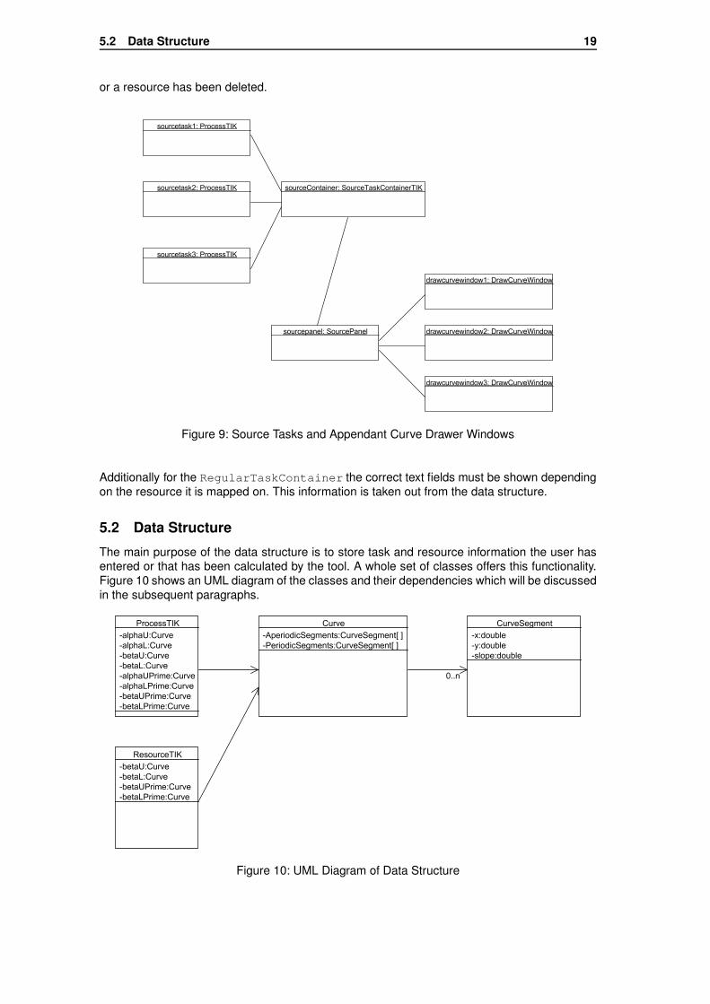
or a resource has been deleted.

Figure 9: Source Tasks and Appendant Curve Drawer Windows

Additionally for the RegularTaskContainer the correct text fields must be shown dependingon the resource it is mapped on. This information is taken out from the data structure.

5.2 Data Structure

The main purpose of the data structure is to store task and resource information the user hasentered or that has been calculated by the tool. A whole set of classes offers this functionality.Figure 10 shows an UML diagram of the classes and their dependencies which will be discussedin the subsequent paragraphs.

Figure 10: UML Diagram of Data Structure


5.2.1 Class Curve

This class represents one curve. This means an instance of this class stores either an upper ora lower curve. The String variable type which can be set to "upper" or "lower" determines thecurve type to be stored.A curve is approximated by a number of linear curve segments as shown in Figure 11 andcan be composed in different ways. It can be periodic, which means the curve is repeated af-ter a period T. On the other side it can be aperiodic, which means the last curve segment isextended to infinity. A combination of these two options is possible, too, but not implementedyet. Depending on whether a curve is periodic or aperiodic the curve segments are stored in aVector AperiodicCurveSegments or in a Vector PeriodicCurveSegments. The periodif needed is saved in the double variable period. The methods isStrictlyPeriodic andisStrictlyAperiodic return true if a curve is strictly periodic respectively strictly aperiodic.If both methods return false, the combination of the two possibilities is used.

Figure 11: Curve Segments of a Staircase Function

The information on how a curve has to be drawn in the grid is saved in this class, too. The wholegrid information including number of squares to be drawn, units per square, curve color andbackground color are saved in the accordant variables. This offers the advantage the user hasto enter the grid properties only once per curve.A curve can be saved to an XML file. This provides the possibility to make the curves portableand to use them in different programs. To save a curve the method saveCurve with the file-name as parameter is used. As this method is public it can be called on every instance of Curveand the user does not need to know about details on saving a curve into an XML file. Dependingon the variable type the curve is saved as upper or lower curve. The library used to write theXML file is JDOM. JDOM allows it to create a well structured XML file in an easy and fast way.Appendix C shows an example of an XML file representing a curve.To load a curve from an XML file an instance of Curve must first be created. Then the methodloadCurve with the name of the XML file can be called and the data is written into the classvariables. In this way it can be automatically recognized if a upper or a lower curve has beenloaded.The method compareCurves is able to compare two curves by comparing each curve seg-ment. If they are equal, the method returns true, otherwise false.The method prune is used to remove unused curve segments and can be applied to everyinstance of Curve.

5.2.2 Class CurveSegment

A curve segment is represented by this class. It can simply store the x and y value of the startingpoint and the slope assigned to the curve segment. Some more methods offer the option toclone a curve segment or to compare it to another one.

5.2.3 Class ProcessTIK

This class represents the different types of tasks. The main idea was to derive it from a genericprocess as described in Section 4.4.2 and in this way make it replaceable with the process class


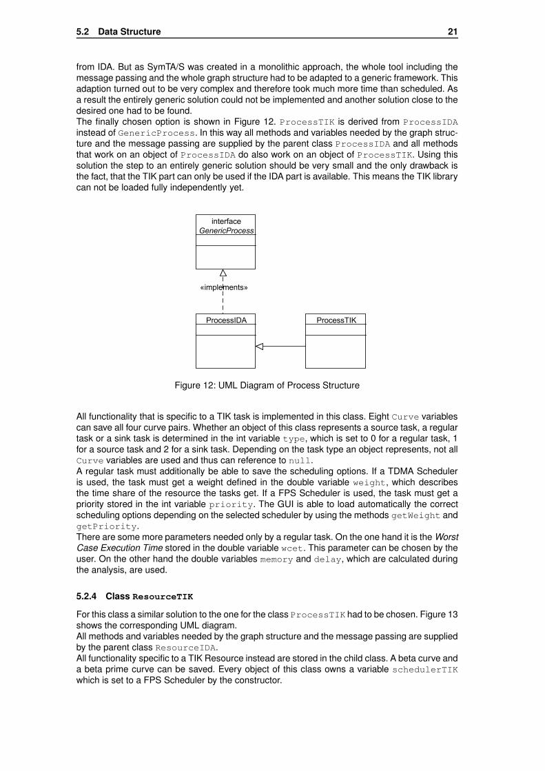
from IDA. But as SymTA/S was created in a monolithic approach, the whole tool including themessage passing and the whole graph structure had to be adapted to a generic framework. Thisadaption turned out to be very complex and therefore took much more time than scheduled. Asa result the entirely generic solution could not be implemented and another solution close to thedesired one had to be found.The finally chosen option is shown in Figure 12. ProcessTIK is derived from ProcessIDAinstead of GenericProcess. In this way all methods and variables needed by the graph struc-ture and the message passing are supplied by the parent class ProcessIDA and all methodsthat work on an object of ProcessIDA do also work on an object of ProcessTIK. Using thissolution the step to an entirely generic solution should be very small and the only drawback isthe fact, that the TIK part can only be used if the IDA part is available. This means the TIK librarycan not be loaded fully independently yet.

Figure 12: UML Diagram of Process Structure

All functionality that is specific to a TIK task is implemented in this class. Eight Curve variablescan save all four curve pairs. Whether an object of this class represents a source task, a regulartask or a sink task is determined in the int variable type, which is set to 0 for a regular task, 1for a source task and 2 for a sink task. Depending on the task type an object represents, not allCurve variables are used and thus can reference to null.A regular task must additionally be able to save the scheduling options. If a TDMA Scheduleris used, the task must get a weight defined in the double variable weight, which describesthe time share of the resource the tasks get. If a FPS Scheduler is used, the task must get apriority stored in the int variable priority. The GUI is able to load automatically the correctscheduling options depending on the selected scheduler by using the methods getWeight andgetPriority.There are some more parameters needed only by a regular task. On the one hand it is the WorstCase Execution Time stored in the double variable wcet. This parameter can be chosen by theuser. On the other hand the double variables memory and delay, which are calculated duringthe analysis, are used.

5.2.4 Class ResourceTIK

For this class a similar solution to the one for the class ProcessTIK had to be chosen. Figure 13shows the corresponding UML diagram.All methods and variables needed by the graph structure and the message passing are suppliedby the parent class ResourceIDA.All functionality specific to a TIK Resource instead are stored in the child class. A beta curve anda beta prime curve can be saved. Every object of this class owns a variable schedulerTIKwhich is set to a FPS Scheduler by the constructor.


Figure 13: UML Diagram of Resource Structure

5.2.5 Interface Drawable

The curve drawer must be able to access curves for editing the classes ProcessTIK andResourceTIK in the data structure. For this reason the interface Drawable has been intro-duced. It is implemented by both classes ProcessTIK and ResourceTIK as shown in Fig-ure 14. The interface guarantees, that the necessary methods to save and store curves areimplemented.The curve drawer accesses the data structure through the interface Drawable using a variableof the type Drawable in the class DrawCurveWindow which can be filled by an object of typeProcessTIK and ResourceTIK.Using this solution the curve drawer can be completely generic and does not have to know if itis used in connection with a process or a resource.

Figure 14: UML Diagram of Interface Drawable

5.3 Analysis 23

5.3 Analysis

The analysis package contains all analysis relevant classes. These are all scheduler classes,the classes, which do the calculation, and the classes, which do the main processing of theanalysis.In this subsection the analysis package is described in detail. But first we provide an explanationhow we run with the calculation through the various tasks that the user has drawn in the editorwindow.

5.3.1 Calculation Flow

Figure 15 shows a simple example with four regular tasks placed on two resources. The tasksT1, T2, T3 and T4 are connected in one line and therefore we call them a Row. The tasks T5,T6, T7 and T8 show the second row. T2 and T6 are mapped on resource R1 which uses thescheduling policy Fixed Priority Scheduling (FPS). T6 has priority 1, whereas T2 has priority2. T3 and T7 are mapped on resource R2 with the scheduling policy Time Division MultipleAccess (TDMA) with a weight of 0.6 respectively 0.4.

T1

T5

T22

T61

T30.6

T70.4

T4

T8

R1:FPS

R2:TDMA

Source Tasks Regular Tasks Regular Tasks Sink Tasks

αT2 α’T2 α’T3αT3

αT6 α’T6 α’T7αT7

Figure 15: Example to Explain the Calculation Flow Implemented in the Library

T1 contains the original alpha curves, T4 holds the resulting alpha prime curves after thecalculation. T2 gets his alpha curves from T1 (αT2) and his beta curves come from theresource. The resulting alpha prime curves of T2 (α′

T2) are the input alpha curves of T3 (αT3).The same can be applied to the tasks in the second row.There are two directions to pass through the tasks. The first direction is along the rows fromthe left to the right. As soon, as the alpha prime curves are calculated, they can be forwardedto the next task and are used there as alpha curves.It may happen that not all curves which are needed for the calculation are available and that wecannot continue from the left to the right. A reason for such an interrupt in the calculation flowcan be seen in Figure 15. The calculation methods starts at T1 and proceeds to the connectedregular task T2 on the right hand. Because we need the resulting beta prime curves on resourceR1 from the regular task with priority 1, we cannot continue our calculation and have to stopit here and first proceed on the second row. Therefore we need the second direction, which isfrom the top to the bottom, or with other words from one row to the next one.

We use a vector to retain the information how fare we could proceed in our calculationflow. The vector contains the references on the tasks which could be successfully handled, forregular tasks this means that all curves could be calculated successfully. The vector containsas many elements as rows exist and is initialized together with the sources.In our example from the former paragraph the first element has not been replaced by areference on T2 because we could not successfully calculate the curves to T2 and it shows thatwe have started with this row and have been stopped at T1 and therefore have to continue there

5.3 Analysis 24

after calculating in row two. In the last paragraphs we have picked out a part at the beginningof the calculation flow. The other tasks are handled in a similar way.We have now introduced the two directions in which we need to proceed our calculation. Thedescription of the implementation of this concept is given in the next subsection.

5.3.2 Class Analysis

The method performAnalysis is described in this paragraph. Figure 16 shows the programflow of this method.

boolean performAnalysis()

- check all parameters

- create Vector (all SOURCE tasks)

- Loop: until Vector contains only SINK tasks

For: Vector size (= number of Rows)

- Test: if actual task is not a SINK

Loop: until error or SINK has been reached

get next task in Row

Test: if REGULAR

- prepare all curves for this new task

-

- if calculation successful -> write new position in Vector

Test: if SINK

- write new position in Vector

(loop)

- Test: if Vector has changed

if not: BREAK! – because of Deadlock!(for)

(loop)

boolean startScheduler()

Calculates alpha and beta prime curves for a given scheduler

boolean totalBetaPrime()

Calculates the total beta curve of a resource

Figure 16: Architecture of the Method Analysis

5.3 Analysis 25

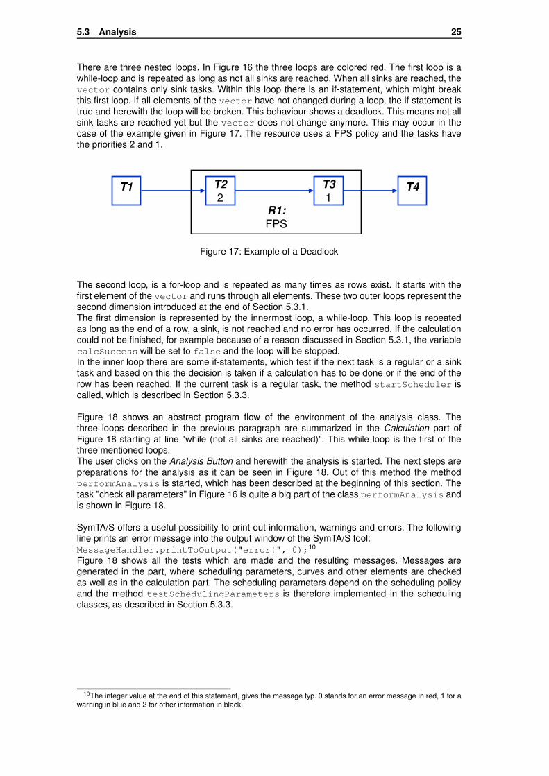
There are three nested loops. In Figure 16 the three loops are colored red. The first loop is awhile-loop and is repeated as long as not all sinks are reached. When all sinks are reached, thevector contains only sink tasks. Within this loop there is an if-statement, which might breakthis first loop. If all elements of the vector have not changed during a loop, the if statement istrue and herewith the loop will be broken. This behaviour shows a deadlock. This means not allsink tasks are reached yet but the vector does not change anymore. This may occur in thecase of the example given in Figure 17. The resource uses a FPS policy and the tasks havethe priorities 2 and 1.

T1 T22

T31

T4

R1:FPS

Figure 17: Example of a Deadlock

The second loop, is a for-loop and is repeated as many times as rows exist. It starts with thefirst element of the vector and runs through all elements. These two outer loops represent thesecond dimension introduced at the end of Section 5.3.1.The first dimension is represented by the innermost loop, a while-loop. This loop is repeatedas long as the end of a row, a sink, is not reached and no error has occurred. If the calculationcould not be finished, for example because of a reason discussed in Section 5.3.1, the variablecalcSuccess will be set to false and the loop will be stopped.In the inner loop there are some if-statements, which test if the next task is a regular or a sinktask and based on this the decision is taken if a calculation has to be done or if the end of therow has been reached. If the current task is a regular task, the method startScheduler iscalled, which is described in Section 5.3.3.

Figure 18 shows an abstract program flow of the environment of the analysis class. Thethree loops described in the previous paragraph are summarized in the Calculation part ofFigure 18 starting at line "while (not all sinks are reached)". This while loop is the first of thethree mentioned loops.The user clicks on the Analysis Button and herewith the analysis is started. The next steps arepreparations for the analysis as it can be seen in Figure 18. Out of this method the methodperformAnalysis is started, which has been described at the beginning of this section. Thetask "check all parameters" in Figure 16 is quite a big part of the class performAnalysis andis shown in Figure 18.

SymTA/S offers a useful possibility to print out information, warnings and errors. The followingline prints an error message into the output window of the SymTA/S tool:MessageHandler.printToOutput("error!", 0);10

Figure 18 shows all the tests which are made and the resulting messages. Messages aregenerated in the part, where scheduling parameters, curves and other elements are checkedas well as in the calculation part. The scheduling parameters depend on the scheduling policyand the method testSchedulingParameters is therefore implemented in the schedulingclasses, as described in Section 5.3.3.

10The integer value at the end of this statement, gives the message typ. 0 stands for an error message in red, 1 for awarning in blue and 2 for other information in black.

5.3 Analysis 26

void run()

Saves curves in unclosed windows

Assigns mapped tasks to resources

Calculation:

If false

Deletes allocation to resources

jbuttonpressed

boolean performAnalysis()

Gets application graph and a list of all processes

User input checking:

for all tasks:SOURCEs:

- checks if all sources have an upper and lower alpha curve

- creates vector with all sources

REGULARs:- sets all betastable flags to false

- checks if every regular task is mapped on a resource

- checks if there is at least one source task in source vector

- checks if all sources lead to a sink& that there is at least 1 regular task in between

- checks if there are unconnected regular or sink tasks

Resources:- checks if all resources have an upper and lower beta curve

Calculation- while (not all sinks are reached)

- at least one sink has not been reached

analysis finished and no error occurred!

Error: no upper/lower curve!

Error: not mapped!

Error: no source around!

Error: no task at output port!Error: no regular between!

Warning: unlinked tasks!

Error: no upper/lower curve!

Error: window size = 0!

Error: total weight > 1!

Warning: total weight < 1!

Error: 2 with same priority!

Info: Analysis started

Info: Analysis stopped

Error: analysis not started!

Warning: deadlock!

boolean startScheduler()

Calculates alpha and beta prime curves for a given scheduler

boolean testScheduling Parameters()

for TDMA:- checks if window size is > 0

- checks total weigth > 1

< 1

for FPS:- checks if all tasks have different priority

Figure 18: Architecture of the Error Handling

5.3.3 Scheduler

The scheduler is related to everything which has to do with the scheduling policy. The UMLdiagram in Figure 19 shows how the scheduler class is embedded into the other classes.There is a general scheduler class, which can be found in the center of the UML dia-gram. This class contains among other methods the three methods called startScheduler,

5.3 Analysis 27

computeFinalBetaPrime and testSchedulingParameters:

startScheduler: This method is called from the method performAnalysis11. The firstpart of the method decides if the calculation on a certain regular task can be done withthe given information, then does prepare all input curves and finally calls the calculationmethods.

computeFinalBetaPrime: Calculates the resulting beta prime curves on each resource andis called at the end of the method performAnalysis.

testSchedulingParameters: This method is designed to test the scheduling parametersand is called from the method performAnalysis.

The methods mentioned above are scheduler dependent and therefore overwritten in theclasses FPSScheduler and TDMAScheduler.

Figure 19: UML Diagram of the Environment of Scheduler Class

For each scheduling policy a separate scheduler class is implemented, which extendsScheduler as Figure 19 shows. Consequently they have to implement the three methodsmentioned above. In Section 5.3.5 and Section 5.3.4 the implementation of the two schedulingpolicies, which have been chosen for the first version of this library, is explained in more details.

The Scheduler contains also the protected Vector relatedTasks, which contains alltasks, which are mapped on one resource and therefore use the same scheduler.A further important variable is parentResource from the type ResourceTIK.parentResource contains a reference to the parent resource the scheduler runs on.The UML diagram in Figure 19 shows these two dependencies.

5.3.4 FPS Scheduler

The implementation of the FPSScheduler class concentrates on the three methodstestSchedulingParameters, startScheduler and computeFinalBetaPrime as ex-plained in the previous paragraph. Partitioned in three paragraphs we will explain the ideasbehind the implementation.

testSchedulingParameters

The FPS policy schedules the order of the tasks based on the priority of each task. The priorityis the only parameter which has to be set and accordingly has to be tested in this method.

11The method performAnalysis is described in Section 5.3.2.

5.3 Analysis 28

The test criteria is, if all tasks on one resource have different priorities.12 The method containstwo nested loops which run through all tasks and compare them to all the other ones. Figure 18contains this error message, too.

startScheduler

The method startScheduler is called out of the method performAnalysis as it can beseen in Figure 16, too. Before invoking the CurveTransform classes, we first have to check ifwe can do the calculation. Therefore we check if this task has the smallest priority. In this case,we get the beta curves directly from the resource and we can start the calculation. If there isa task with a smaller priority, than the current one gets the beta curves from the previous one.But first we have to check if the beta curves of the previous one are already calculated correctly.The method getStableBetaPrime() called on the the previous task tells us if these betacurves can be used or not. If we cannot use these beta curves, what means, that the task withthe smaller priority has not been calculated, we cannot do a calculation step and return false.Otherwise we get the beta curves from the previous task and start the analysis.

computeFinalBetaPrime

With FPS the resulting beta prime curves on a resource are the beta prime curves of the taskwith the lowest priority running on it. Therefore this method checks all task on this resource andstores the beta curves of the task with the lowest priority in the resource class.

5.3.5 TMDA Scheduler

The structure of the TDMAScheduler class is similar to the FPSScheduler class.

testSchedulingParameters

When the user chooses a TDMA scheduling policy, the parameter which reallocates the re-source is the weight of a task. The total weight is normally 1.0. This method adds all weights ona resource up and checks the result. If the totalized weight is greater than 1.0, the analysis willbe stopped. If it is smaller then 1.0 a warning will be printed out.13

The second parameter which has to be tested is the window size. The window size has to begreater than 0.0 if the window size is evaluated, otherwise we do not care about the enteredvalue.

startScheduler

The resource capability is split based on the weight. Therefore a calculation can always bestarted, contrary to the FPS scheduler.There are two possible scenarios now. The first one is, that we evaluate the window sizeand calculate the weighted beta curves regarding the window size. Such curves can be seenin Figure 20.14 On the other hand the user can choose to weight the beta curves withoutevaluating the window size, which can be seen in Figure 21.

After having finished the preparation of all needed curves we can calculate the curves usingagain the methods of the CurveTransform class.

computeFinalBetaPrime

If we have not evaluated the window size, we can calculate a beta prime curves, which are thesum of all beta prime curves on this resource. Otherwise the tool does not calculate a resultingbeta prime curves.

12The analysis is only started, if there are no task on a resource with the same priority. Otherwise the analysis wouldnot work properly.

13A totalized weight of smaller then 1.0 means that there are other tasks which run on this resource, which are notdrawn here.

14The method accepts for the case "evaluate window size" only curves which consist of exactly one curve segment.

5.3 Analysis 29

Figure 20: Weighted Beta Curves withthe Option Evaluate Window Size anda Window Size of 1.0

Figure 21: Weighted Beta Curveswithout the Option Evaluate WindowSize

5.3.6 Class WCET_calculation

The class WCET_calculation is a very simple class and consists only of two methods. TheWorst Case Execution Time (WCET) influences the alpha curves and the resulting alpha primecurves as described in Section 2.3.2.The current version of the library provides the possibility to enter a value for the WCET for eachtask. The two methods in this class provide multiplication and division of an alpha curves withthis chosen WCET value. They are called out of the scheduler, the multiplication at the beginningand the division at the end of the calculation process.

5.3.7 Package Singlenode

The package ch.ethz.ee.tik.rtc.analysis.singlenode contains all classes whichdo calculations based on the TIK analysis method on a single node. The most important classis the CurveTransform class, which can be used to call calculations. The other classes areonly used within the package.

The class CurveTransform contains the following methods:

getLowerArrivalPrime(...) returns the lower alpha prime curves based on the alphalower, beta lower and beta upper curves.

getUpperArrivalPrime(...) returns the upper alpha prime curves based on the alphaupper, beta lower and beta upper curves.

getLowerServicePrime(...) returns the lower beta prime curves based on the beta lowerand alpha upper curves.

getUpperServicePrime(...) returns the upper beta prime curves based on the beta up-per and alpha lower curves.

getDelay(...) returns the delay of a node based on the alpha upper and beta lower curves.

getMemory(...) returns the memory consumption of a node based on the alpha upper andbeta lower curves.

addCurves(...) can be used to add two curves.

multCurve(...) can be used to scale curves with a factor.

This package has not been implemented by us and we therefore do not explain any furtherdetails.

6 Short user manual 30

6 Short user manual

6.1 How To Use?

This section will give a short introduction on how to use SymTA/S focusing on the new featuresthat have been added by the TIK library.

6.1.1 Tasks and Resources

The user has the possibility to add three different tasks by clicking on the appropriate icon in thetool bar:

• a source task,

• a regular task,

• and a sink task.

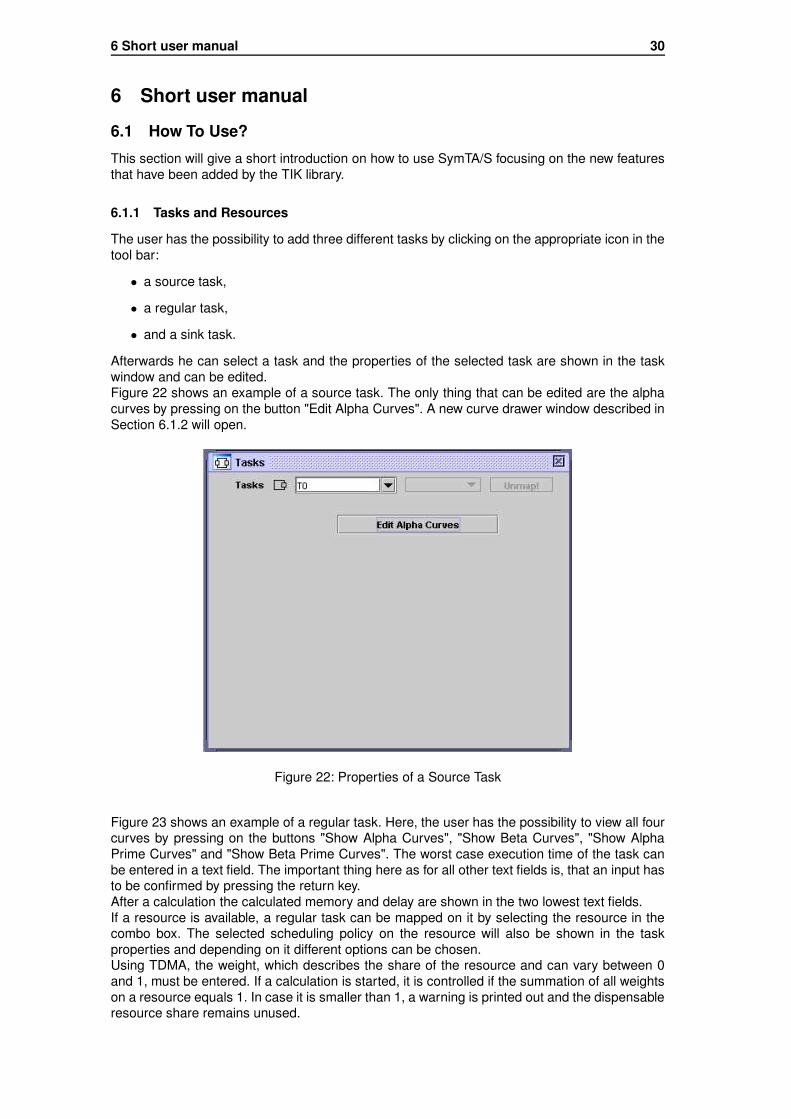
Afterwards he can select a task and the properties of the selected task are shown in the taskwindow and can be edited.Figure 22 shows an example of a source task. The only thing that can be edited are the alphacurves by pressing on the button "Edit Alpha Curves". A new curve drawer window described inSection 6.1.2 will open.

Figure 22: Properties of a Source Task

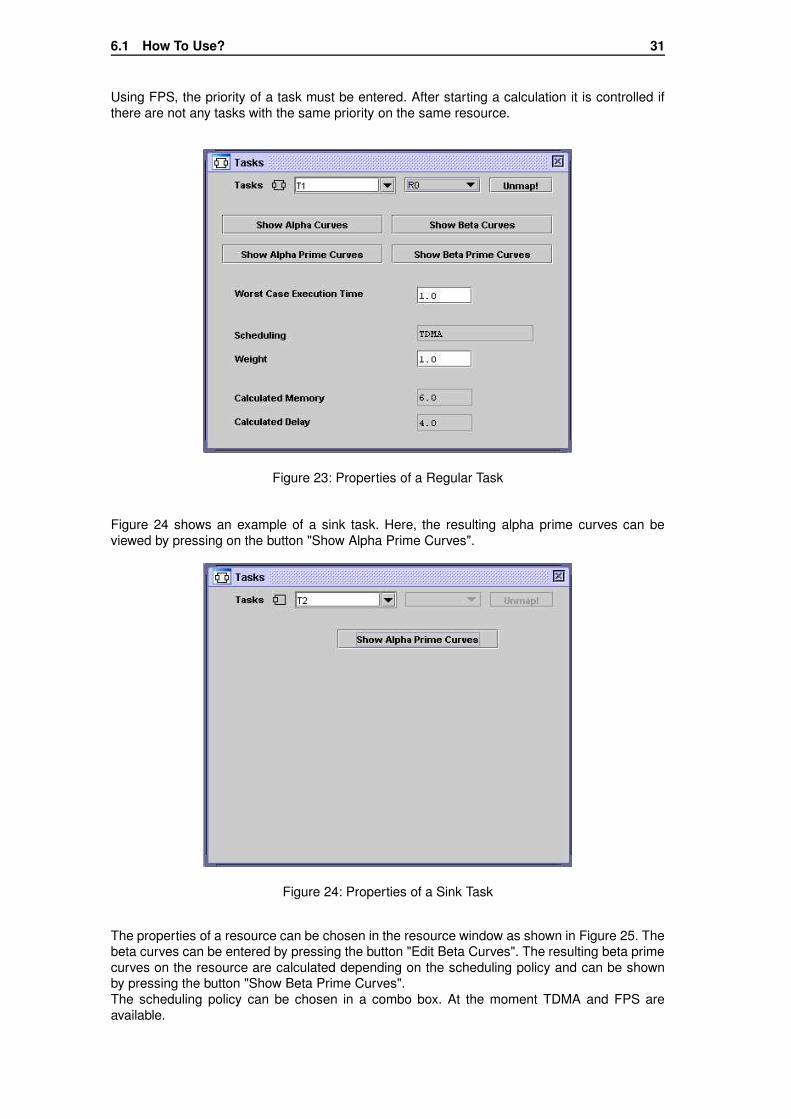
Figure 23 shows an example of a regular task. Here, the user has the possibility to view all fourcurves by pressing on the buttons "Show Alpha Curves", "Show Beta Curves", "Show AlphaPrime Curves" and "Show Beta Prime Curves". The worst case execution time of the task canbe entered in a text field. The important thing here as for all other text fields is, that an input hasto be confirmed by pressing the return key.After a calculation the calculated memory and delay are shown in the two lowest text fields.If a resource is available, a regular task can be mapped on it by selecting the resource in thecombo box. The selected scheduling policy on the resource will also be shown in the taskproperties and depending on it different options can be chosen.Using TDMA, the weight, which describes the share of the resource and can vary between 0and 1, must be entered. If a calculation is started, it is controlled if the summation of all weightson a resource equals 1. In case it is smaller than 1, a warning is printed out and the dispensableresource share remains unused.

6.1 How To Use? 31

Using FPS, the priority of a task must be entered. After starting a calculation it is controlled ifthere are not any tasks with the same priority on the same resource.

Figure 23: Properties of a Regular Task

Figure 24 shows an example of a sink task. Here, the resulting alpha prime curves can beviewed by pressing on the button "Show Alpha Prime Curves".

Figure 24: Properties of a Sink Task

The properties of a resource can be chosen in the resource window as shown in Figure 25. Thebeta curves can be entered by pressing the button "Edit Beta Curves". The resulting beta primecurves on the resource are calculated depending on the scheduling policy and can be shownby pressing the button "Show Beta Prime Curves".The scheduling policy can be chosen in a combo box. At the moment TDMA and FPS areavailable.

6.1 How To Use? 32

If TDMA is selected, two different calculation models are supported. The first model evaluatesthe window size, the second one does not.

Figure 25: Properties of a Resource

6.1.2 Curve Drawer

Figure 26 shows an example of an editable curve drawer window. All icons in the tool bar fromthe left to the right are described in this paragraph.

Figure 26: Curve Drawer Window

Curves can be painted by selecting the icons "Draw Upper Curve" or "Draw Lower Curve".

6.2 Analysis Example 33

Afterwards a single curve segment or a set of curve segments can be selected, if the "select"icon is active. The selected elements can be moved or deleted by pressing the "Delete" icon.The "Grid Properties" icon allows to change the grid properties in a new window.The next four icons are used to load and save curves to an XML file or to save the curves as ascreen shot into a png file.In the radio button group it is decided, whether a the curves are periodic or aperiodic. If periodicis selected, the period text field becomes editable.The check box "Show Positions" allows tho show the positions of the mouse cursor and allselected curve segments.By clicking on the "Close Window" icon or the cross icon in the upper right corner the windowis closed and the curves are saved to the data structure. If a curve is loaded from the datastructure and shown in the curve drawer window, the last curve segment gets automatically thelength 1 in the x direction, because the ending point is not defined.

6.2 Analysis Example

In this section an example of a simulation which has been done using the new TIK library willbe presented. Figure 27 shows the structure of the tasks and resources.

Figure 27: Simulation Example

T1 uses the alpha curves shown in Figure 28. T3 uses the alpha curves shown in Figure 29.

Figure 28: Alpha Curves Task T1


Figure 29: Alpha Curves Task T3

R0 has the following properties:

• FPS Scheduler

• mapped tasks: T1, T4

• priority T1: 1

• priority T4: 2

• beta curves shown in Figure 30

Figure 30: Beta Curves Resource R0 and R1 (Upper and lower curves are congruent.)

R1 has the following properties:

• TDMA Scheduler

• mapped tasks: T6, T7

• weight T6: 0.5

• weight T7: 0.5


• evaluate: not selected

• beta curves shown in Figure 30

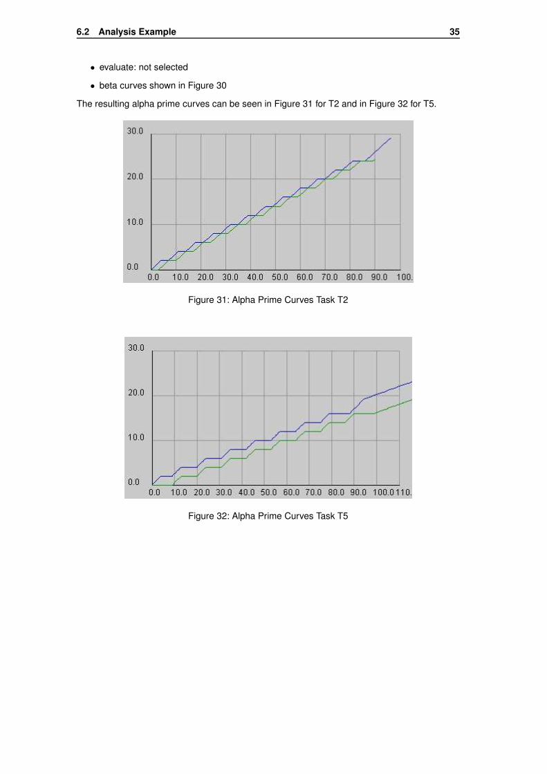
The resulting alpha prime curves can be seen in Figure 31 for T2 and in Figure 32 for T5.

Figure 31: Alpha Prime Curves Task T2

Figure 32: Alpha Prime Curves Task T5

7 Outlook 36

7 Outlook

The generic approach of the solution which has been pursued offers the possibility to improvethe tool.

The first step that will surely have to be taken is the implementation of the completelygeneric data structure. As soon as the generic framework is available, it should be possibleto adapt the concerned classes in an easy manner. As the data structure classes are alreadyprepared for this solution, some small changes will be necessary.

Probably, new scheduling policies will be desired. In this case a new class derived fromScheduler can be added and the methods specific to the new scheduling policy must beoverwritten. Some modification in the GUI container for the resource will also be necessary,but totally the modifications should be very small as the structure of the resource is alreadyprepared to add new schedulers.

A further problem to deal with is the improvement of the calculation performance. Simu-lations have shown, that a calculation can take a not negligible amount of time. An optimizationof the calculation algorithms or a limitation to a certain number of curve segments which is notdefined yet would surely improve the performance.

8 Summary 37

8 Summary

During this thesis a library to the SymTA/S tool has been developed to use the Real TimeCalculus methods efficiently. A generic approach has been almost totally implemented.Therequirements on the library could be fulfilled and the two scheduling policies Fixed PriorityScheduling and Time Division Multiple Access have been implemented successfully.

The program contains a useful tool to draw curves. The curves drawn can be used forthe analysis or be stored into XML files to use them in other programs. The major part of thework was to design a userfriendly solution and to develop a comprehensive error handling.

The current version of the library provides a stable solution which can be used to gainfirst experiences with this new tool.

A Acknowledgements 38

A Acknowledgements

Various helpful comments and ideas were received from Simon Künzli.

Furthermore, mainly lively discussions with colleagues created input to the work.

B Bibliography / References 39

B Bibliography / References

References

[1] S. Chakraborty, S. Künzli, and L. Thiele,A general framework for analysing system properties in platform-based embedded systemdesigns.;Proc. 6th Design, Automation and Test in Europe (DATE), pages 190 - 195, Munich, Ger-many, March 2003.

[2] S. Chakraborty, S. Künzli, and L. Thiele, A. Herkersdorf, and P. Sagmeister,Performance evaluation of network processor architectures: Combining simulation with an-alytical estimation.;ComputerNetworks, 41(5): 641 - 665, April 2003.

[3] C. L. Liu and James W. Layland,Scheduling algorithms for multiprogramming in a hard-real-time environment.;J. ACM, 20(1):46-61, 1973.

[4] A. Maxiaguine, S. Künzli, and L. Thiele,Workload characterization model for tasks with variable execution demand.;Proc. 7th Design, Automation and Test in Europe (DATE), pages 1040 - 1045, Paris,France, February 2004.

[5] Kai Richter, Marek Jersak, and Rolf Ernst,A formal approach to mpsoc performance verification.;Computer, 36(4): 60 - 67, 2003.

[6] Kai Richter, Razvan Racu, and Rolf Ernst,Scheduling analysis integration for heterogeneous multiprocessor SoC.;Proceedings of the IEEE Real-Time Systems Symposiums (RTSS), Cancun, Mexico, 122000. IEEE Computer Society.

[7] L. Thiele, S. Chakraborty, M. Gries, and Simon Künzli,Design spaces exploration of network processors architectures.;Mark Frankling, Patrick Crowley, Haldung Hadimioglu, and Peter Onufryk, editors, NetworkProcessor Design Issues and Practices, Volume 1, chapter 4, pages 55 - 90. Morgan Kauf-mann, October 2002. A preliminary version of this paper appeared in the Proc. 1st Work-shop on Network Processors, held in conjunction with the 8th International Symposium onHigh-Performance Computer Architecture, Cambridge, Massachusetts, 2002.

[8] flowspec.dtd;available at http://www.tik.ee.ethz.ch/˜ kuenzli/dtds/flowspec.dtd, April 2004.

[9] libpreferences.xml;document within source folder: /src/org/spiproject, March 2004.

[10] Institute IDA at TU Braunschweig,SymTA/S project webpage.;http://www.ida.ing.tu-bs.de/research/projects/symta-s/home.g.shtml, May 2004.

[11] Institute IDA at TU Braunschweig,Symta System, Quick Reference for advanced user;http://www.ida.ing.tu-bs.de/research/projects/symta-s/home.g.shtml, May 2004.

C Example of a Curve XML File 40

C Example of a Curve XML File

The example below shows an XML file of an upper curve, as it has been stored in the CurveDrawer Window.

<?xml version="1.0" encoding="UTF-8"?><curvecontainer xunit="1.0" yunit="1.0" xgrid="10" ygrid="10"><curve name="uppercurve" type="upper">

<aperiodic burstlength="0.0"><curvesegment x="0.0" y="2.0" slope="0.0" /><curvesegment x="11.0" y="4.0" slope="0.0" /><curvesegment x="22.0" y="6.0" slope="0.0" /><curvesegment x="33.0" y="8.0" slope="0.0" /><curvesegment x="44.0" y="10.0" slope="0.0" /><curvesegment x="55.0" y="12.0" slope="0.0" /><curvesegment x="66.0" y="14.0" slope="0.0" /><curvesegment x="77.0" y="16.0" slope="0.0" /><curvesegment x="90.0" y="18.0" slope="0.18181818182" />

</aperiodic><periodic period="0.0" />

</curve></curvecontainer>

D Libpreferences.xml

The Libpreferences.xml file defines which modules are used as described in Section 4.

<?xml version="1.0" encoding="UTF-8"?>

<Symta-S>

<gui>

<RegularTaskContainer>ch.ethz.ee.tik.rtc.gui.RegularTaskContainerTIK

</RegularTaskContainer><SourceTaskContainer>

ch.ethz.ee.tik.rtc.gui.SourceTaskContainerTIK</SourceTaskContainer><SinkTaskContainer>

ch.ethz.ee.tik.rtc.gui.SinkTaskContainerTIK</SinkTaskContainer><ResourceContainer>

ch.ethz.ee.tik.rtc.gui.ResourceContainerTIK</ResourceContainer><EventStreamContainer>

ch.ethz.ee.tik.rtc.gui.EventStreamContainerTIK</EventStreamContainer>

</gui>

<datastructure>

<GenericProcess>ch.ethz.ee.tik.rtc.datastructure.ProcessTIK

</GenericProcess><GenericResource>

ch.ethz.ee.tik.rtc.datastructure.ResourceTIK</GenericResource><GenericInputPort>

org.spiproject.lib.datastructure.InputPortIDA</GenericInputPort><GenericOutputPort>

org.spiproject.lib.datastructure.OutputPortIDA</GenericOutputPort><GenericEventStream>

org.spiproject.lib.datastructure.EventStreamIDA</GenericEventStream><GenericEventModel>

org.spiproject.lib.datastructure.EventModelIDA</GenericEventModel>

</datastructure>

<analysis>

<GenericAnalysis>

org.spiproject.lib.analysis.AnalysisIDA</GenericAnalysis>

</analysis>



<settings>

</settings>

</Symta-S>

report - pub.tik.ee.ethz.ch · 1 abstract a analysis method for embedded systems, called real time...

Documents