Report on Evaluation Experiments Using DifferentMachine Learning Techniques for Defect Prediction

Marios GrigoriouDept. of Computer Science

Western UniversityLondon, ON. Canada

mgrigori@uwo.ca

Kostas KontogiannisDept. of Computer Science

Western UniversityLondon, ON. Canada

kostas@csd.uwo.ca

Alberto GiammariaIBM

IBM Austin LaboratoryAustin TX. USA

agiammaria@us.ibm.com

Chris BrealeyIBM

IBM Toronto LaboratoryToronto ON. Canadacbrealey@ca.ibm.com

Abstract—With the emergence of AI, it is of no surprise thatthe application of Machine Learning techniques has attracted theattention of numerous software maintenance groups around theworld. For defect proneness classification in particular, the useof Machine Learning classifiers has been touted as a promisingapproach. As a consequence, a large volume of research workshas been published in the related research literature, utilizingeither proprietary data sets or the PROMISE data repositorywhich, for the purposes of this study, focuses only on the use ofsource code metrics as defect prediction training features. It hasbeen argued though by several researchers, that process metricsmay provide a better option as training features than source codemetrics. For this paper, we have conducted a detailed extractionof GitHub process metrics from 150 open source systems, andwe report on the findings of experiments conducted by usingdifferent Machine Learning classification algorithms for defectproneness classification. The main purpose of the paper is notto propose yet another Machine Learning technique for defectproneness classification, but to present to the community a verylarge data set using process metrics as opposed to source codemetrics, and draw some initial interesting conclusions from thisstatistically significant data set.

Index Terms—Machine learning, software maintenance, defect-proneness, experiments, data set, open source systems.

I. INTRODUCTION

The problem of classifying a file as failure prone or not hasattracted the attention of the software engineering communityearly on. Early approaches focused on the use of softwaremetrics to compute maintainability and software health indexes[19] [20]. These approaches were based on the compilation oflinear or non-linear formulas to yield maintainability indexeswhich were assumed to be associated with the overall health ofa component or a system. In this respect, the assumption wasthat a higher maintainability index would indicate a softwarecomponent (function, method, file, or module) that has a lowprobability of exhibiting a failure. As research progressed inthis field, the software engineering community experimentedwith approaches focusing on the static and dynamic analysisas well as the analysis of project data, such as the number,type and time interval between bug fixes [24] [25]. Theseapproaches utilized statistical analyses and heuristics to ex-perimentally yield predictions related to the fault-pronenessof a software component. However, over the past few years,research in this area has decisively shifted towards the use of

Machine Learning (ML) techniques. These techniques aim tofirst identify a collection of source code related and processrelated features which can serve as classiffiers for fault-proneness, and second apply these features for training MLmodels using a variety of ML algorithms (see Section II). Oncesuch models are trained they can be used to classify whethera newly seen software component is defect prone or not.

The challenge that arises using such ML techniques is thatthey yield models which perform as black boxes and donot provide any explanation on how their results have beenreached, as they are purely dependent on the training data setprovided, and the ML algorithm used. Another challenge thatarises is when ML models are trained on source code metricsalone. Large software systems are rarely implemented usinga single programming language and are often composed of acollection of different frameworks, configuration scripts anddynamically linked components. That makes the extraction ofaccurate source code metrics an almost impossible task. Onthe contrary, process related metrics can be extracted quiteaccurately and easily from various DevOps tools such asGitHub, Jira, Jenkins, and Slack.

This paper aims to shed light on two major issues.The firstissue is to identify, through the use of process metrics andextensive experimentation, the technique, or the combinationof techniques and features, that best classify whether a soft-ware component (i.e. file) can be considered defect proneor not. The second issue is whether process metrics can beused instead of source code metrics and whether these can beused to train models that yield similar of better classificationresults in a single project or across projects. These issues areformalized by the following research questions:

RQ1: By using a very large set of open source projectsto experiment with, which is the best combination ofclassifiers which are fast, easily trainable and able toyield the best results as these are measured in terms ofaccuracy, precision, recall, F1, and AUC?

RQ2: What is an optimal subset of available process metricswhich can be easily calculated and at the same timeyield the best results when provided as input to differentclassifiers?

RQ3: Is it possible to perform defect-proneness classificationusing process metrics while maintaining classificationperformance measures comparable to similar techniquesreported in the literature which use source code metrics?

RQ4: Is it possible to perform cross project defect pronenessclassification in the sense that data from different projectscan be used to train a model which will then be used toperform defect proneness prediction on other unknownprojects for which not enough training data may beavailable?

For this paper we take an experimental approach, aimingto draw conclusions by applying the techniques under exam-ination to a very large collection of open source projects.More specifically, we have considered a collection of 150open source systems from which we have extracted variousprocess metrics utilising a custom-made extraction tool. Theopen source projects were selected based on their complexity,size, prevalence, and the quality and availability of processrepository data. The importance of the work reported in thispaper lies on two parts. First, in the best of our knowledge, itis the first work which utilises such a large data set, providingthus a much more statistically significant result than previouslyreported works, and second providing answers to researchquestions which can assist researchers advance the state-of-the-art in the area.

The paper is organised as follows. Section II presentsrelated work. Section III discusses the features and the featureextraction process. Section IV presents the different MachineLearning techniques which we have evaluated. Section Vpresents the results obtained, while Section VI discusses andinterprets the obtained results. Finally, Section VII concludesthe paper and offers pointers for future work.

II. BACKGROUND

In the related literature there is a wealth of approaches fordefect prediction using Machine Learning techniques. Twowidely-used defect prediction techniques are regression andclassification. The main purpose of regression techniques isto estimate the number of software defects on a softwarecomponent. In contrast, classification techniques aim to tagwhether a software module is faulty or not. It has been shownthat classification models can be trained from defect data onearlier versions of the system being analyzed. Some of themost commonly used supervised learning techniques for defectprediction are outlined below.

Decision Trees (DT): Decision tree algorithms use treestructures to model decisions and their possible consequences.In decision trees each leaf node corresponds to a class labelwhile attributes are represented as internal tree nodes.

Logistic Regression (LR): Logistic regression is a supervisedclassification algorithm whereby the target variable O (i.eoutput), can take on values in the interval [0, 1] representingthe probability for a given set of input features I to belong toclass 1 or 0.

Random Forest (RF): RF is an ensemble type of learningmethod used for both classification and regression problems.The key idea behind RF is the construction of several decisiontrees at training time and outputting the mode/mean predictionof the individual trees.

Support Vector Machine (SVM): SVM is a discriminativeclassifier formally defined by a separating hyperplane. InSVMs, given a labeled training data set whereby each dataitem is marked as belonging to one or the other of twocategories, the algorithm outputs an optimal hyperplane, whichclassifies new unseen data in one of these two categories.

k-Nearest Neighbors (k-NN): k-NN is a non-parametricmethod that can be used for both classification and regressionproblems. In both cases, the input consists of the k closesttraining examples in a feature space. The output dependson whether k-NN is used for classification or regression. Inclassification, the output is to categorize an input to one ofequivalence classes. In regression, the output is to assign avalue to the input, usually the average of the values of itsclosest k-neighbors.

Naive Bayes Classifiers (NB): These classifiers refer to afamily of simple ”probabilistic classifiers” based on applyingBayes’ theorem and by considering a strong independenceassumption between features, that is the presence or absenceof a particular feature of a class is not related to the presenceor absence of any other feature.

Neural Networks (NN): Neural Networks are nonlinearpredictive structures that consist of interconnected processingelements called neurons that work together in parallel withina network to produce output, often simulating an unknownfunction or phenomenon.

Multi-layer Perceptron (MLP): MLPs refer to a class offeedforward artificial neural network (ANN). An MLP com-prised of a directed graph of multiple layers of nodes whichare fully connected to the nodes of the next layer. For trainingpurposes, MLP utilizes a supervised learning technique definedas backpropagation.

Radial Basis Function (RBF) Networks: RBF Networks area type of ANNs used to approximate through training the valueof an unknown function. They are different from MLPs in thesense that they are feedforward networks comprising of onlythree layers, the input layer, the hidden layer and the outputlayer.

A. Defect Prediction using Machine Learning

A variety of machine learning methods have been proposedand assessed for addressing the software bug prediction prob-lem. These methods include decision trees [4], neural networks[8], [12], Naive Bayes [7], [11], [17], support vector machines[6], Bayesian networks [16] and Random Forests [9].

1) Source CodeMetrics Approaches: Deciding whether acomponent has a high likelihood to be defective or not hasbeen proved to have a strong correlation with a number ofsoftware metrics. Identifying and measuring software metricsis vital for various reasons, including estimating program

execution, measuring the effectiveness of software processes,estimating required efforts for processes, estimating the num-ber of defects during software development as well as mon-itoring and controlling software project processes [21] [22].Various software metrics have been commonly used for defectprediction, including lines of code (LOC) metrics, McCabemetrics, Halstead metrics, and object-oriented software met-rics. Hence, the automated prediction of defective componentsfrom extracted software metrics evolved as a very activeresearch area. [36]. In [14], Nagappan aims to find the bestcode metric to predict bugs. The conclusion of this work isthat complexity metrics can successfully predict post-releasedefects, but there is no single set of metrics that is applicableto all systems. Hassan et. al have investigated the impact ofdifferent aspects of the modelling process to the end resultsand the interpretation of the models [28] [29] [30] [31] [40].

2) Process Metrics Approaches: In [10], Venkata et. alcompared different machine learning models for identifyingfaulty software modules and they found that there is no par-ticular learning technique that performs the best for all the datasets. In [5], Wang and Yao aim to find bugs without decreasingthe overall performance of the model. In this process, they findthat imbalanced distribution between classes in bug predictionis the root cause of its learning difficulty. Likewise, in ourpaper, we noted the issue and used re-sampling as described indetail in the section IV-C in an effort to minimise the impact ofclass imbalance to the quality of our results. Similarly, in [15],Zimmermann et. al propose an approach to predict bugs oncross-language systems. The work examined a large number ofsuch systems and concluded that only 3.4% of the systems hadprecision and recall prediction levels above 75% . The authorsalso tested the influence of several factors on the success ofcross-language prediction and concluded that there was nosingle factor which led to such successful predictions. Theauthors used decision trees to train the model and to estimateprecision, recall, and accuracy before attempting a predictionacross systems. Lastly, in [13], Hassan discusses how frequentsource code “commits” in the repository negatively affect thequality of the software system, meaning that the more changesincurred to a file, the higher the chance that the file will containcritical errors. Furthermore, the author in [13] presents a modelwhich can be used to quantify the overall system complexityusing historical code-change data, instead of plain source codefeatures.

III. DATA MODELING

For the purposes of this study we have designed twoseparate data models. The first data model denotes the rawinformation which can be mined from software repositories,while the second data model denotes the post-processed rawdata which are in a form that can be consumed by the machinelearning algorithms we have experimented with.

The design goal of the first data model was to have astructure which would be easy to populate while maintaining alow memory profile, would facilitate data reconciliation of data

Fig. 1. Data Model for Raw Repository Data

entries originating from different devOps tools (e.g. GitHub,Jenkins, Jira), would be scalable, and would be able to supportpreprocessing workflows of varying complexity at high speeds.The schema for this data model is depicted in Fig. 1.

The design of the second data model was to have a simplerelational structure which can be easily imported as a tab orcomma delimited file in various machine learning tools andwhich can be easily manipulated so that aggregate features canbe easily computed. The features in this second data model aredepicted in Table I.

A. Raw Data Model

For this study we have exhaustively collected process relatedmetrics from 150 open source systems of various sizes andcomplexities. The list of the systems along with all the dataobtained or computed are listed in the anonymous repository[23].1 The profile of the data set we have considered isdepicted in Table II. The data acquisition process is based ontwo steps. The first step is to utilize a custom made client-sideextractor tool which is able to connect to and reconcile dataobtained using various tools and namely GitHub, Bugzilla,Jira, and Jenkins. However, for this study we report resultson data acquired only from the GitHub repositories of these150 open source systems. The second step of the raw dataacquisition process is to fuse the information extracted by eachrepository record into one repository which conforms to theraw data schema depicted in Fig. 1. The extractor applicationand its data fusion module is implemented using Python 3.

1Please note that the repository is anonymous for the time being, in orderto protect the double blind review process and to facilitate the assessmentof this work by the reviewers. Please do not distribute or use without priorarrangements with the authors.

As depicted in Fig. 1, the raw data model is founded on theconcept of a Commit, the concept of a File, and the concept ofa CommitProperties. The extracted information is representedas a Json file stored in a Mongo DB server. As such, a run-time model of a GitHub repository was created which heldthe information of the unique commit records. Every commitcontained a list of fileChanges and the details for each of thesefiles’ change. This data model represents a GitHub recordstructure utilizing simple Python 3 objects which have a verylow memory profile and initialization time.

In this data model a commit is uniquely identified by it’scommitID, it contains attributes specific to it, including theauthor, the commit-time, the files committed as these aredenoted by their FileIds, a commit message, the overall linesadded, deleted as well as a tag field maintaining informationabout whether the Commit’s status is indicated as a bug fixingor as a clean Commit. For each File within a commit, theadded, and deleted lines as well as the current size of thefile are maintained. Storing the fileID is necessary since incase of a file changing locations the fileID remains the sameeven if the file changes name (the names are fully qualifiednames with respect to the root folder of a project). In additionto the version control model, another important componentof this extractor system is the issue tracker component. Thiscomponent is far simpler. It is a simple object maintaining aspecific issueID together with the issue tag its message and itsreferenced commitIDs. The data model is populated by initiallydownloading a complete repository from the correspondingGitHub site and then moving through each commit on themaster branch adding the relative data iteratively in it, thusmaintaining the initial structure. Once the model is populatedit undergoes several steps of preprocessing. The first task isto remove all files that cannot contribute to a defect, suchas any non-compilable and non-configuration related files.The next task is to use a simple heuristic to clean up theextracted commits so that only actual code changing commitsremain. This entails removing all commits that are clearlyannotated as a refactoring commit, and also removing allfiles which have been eventually removed from the systemfrom all past commits. Finally all merge commits are alsoremoved since they contain change information pertaining todifferent branches and will therefore introduce large ammountof noisy data points to the dataset. Given that this studyis not focusing on defect introducing software changes, theremoval of refactoring and merge commits from the datasetwill not impact its ability to discern between faulty and healthyfiles. After the cleanup stage is completed, the most importantremaining task is that of assigning the class label for eachcommit. This task is accomplished by parsing the commitmessage for terms that may indicate that it is a bug-fixingcommit as opposed to a clean one, linking commits to issuetracker entries labeled as faults and optionally, applying thesame parsing as above to the issue tracker messages. Theheuristic terms used to tag a commit as a bug-fixing oneare presented in Section IV-B below. This is an approachfor automatically generating datasets for such applications

TABLE IFEATURES USED FOR SYSTEM TRAINING

F1: NoOfCommits (CF) F2: LateNightCommits (LNC)F3: TotalAddedLines (TAL) F4: MaxAddedLines (MAL)F5: AvgAddedLines (AAL) F6: TotalDeletedLines (TDL)F7: MaxDeletedLines (MDL) F8: AvgDeletedLines (ADL)F9: TotalChurn (TCF) F10: MaxChurn (MC)F11: AvgChurn (AC) F12: TotalCoCommitSize (TCS)F13: MaxCoCommitSize (MCS) F14: AvgCoCommitSize (ACS)F15: TotalDistinctAuthors (TDA) F16: AgeInMonths (AIM)F17: FractalValue (FRV) F18: FailureIntensity (FI)

which has been known to work in the related literature [26].This approach however has the potential to produce a highnumber of false positives in the dataset because of the commitgranularity level at which it is applied. This is due to the factthat some commits may be only partially defective leading towrong labels for the non-defective part [39]. In this case theentirety of the commit and its modifications are annotated asbug-fixes, which is not acceptable for commits that contain asignificant percentage of a systems’ files.

B. Post-Processed Data Model

Once the raw data are extracted they are post-processedin order to yield a data model suitable for input to variousMachine Learning classification tools. Table I provides a listof the features considered for our study.

C. Explanation of the Features

The FractalValue [27] provides a measure for the contribu-tion of different authors to a file. It can take any value in therange (0, 1] where a value of 1 means that a file has had asingle author whereas a value close to 0 means that the filehas had similar contributions from multiple different authors.TotalCoCommitSize for a file Fi in a system S is the countof all files Fj ∈ S which have been committed alongside Fi,counting multiple occurrences of the same files.

IV. MACHINE LEARNING FRAMEWORK

In this section we discuss the machine learning algorithmsused and technical details on how training and testing wereconducted for this study.

A. Machine Learning Models Considered

For our experiments we have considered six different clas-sification algorithms, and namely (1) Logistic Regression; (2)Support Vector Machines; (3) Multi-Layer Perceptron; (4)Decision Trees; (5) Random Forests and; (6) Naı̈ve Bayes.The selection of these algorithms is based on the fact thatthese are the algorithms most commonly used in the relatedliterature [38], [35], [36] [37].

Each of the aforementioned algorithms comes with its ownbenefits and drawbacks. The most important benefit was thespeed at which these can be trained and evaluated while themost important drawback of all approaches except for LogisticRegression was the lack of explainability. Nevertheless, thecombination of these algorithms is currently the de-factostandard in the related literature as base classifiers [36] [38].

B. Commit Tagging

As discussed in Section III-B the raw data repository isconsidered as a container of commits. Each commit is taggedin the repository as a bug fixing commit or a clean commit.This tagging is based a) on the label of the GitHub commitrecord itself, or in the absence of such a label by analyzingthe comments section of the commit record. More specifically,if the comments section of the commit record contains any ofthe keywords ’bug’, ’bugs’, ’defect’, ’defects’, ’error’, ’errors’’fail’, ’fails’, ’failed’, ’failing’, ’failure’, ’failures’, ’fault’,’faults’, ’fix’, ’fixes’, ’fixed’, ’fixing’, ’problem’, ’problems’,’wrong’ which may indicate a bug fixing intention, then thecommit is tagged as a buggy commit (label 1), otherwise as aclean commit (label 0).

C. File Tagging

In its turn, a commit is considered itself as a container offiles. If a commit is tagged as a bug fixing one (see above),then all the files in the commit are also tagged as buggy.This is a heuristic that can introduce many false positives,but unfortunately in the absence of a gold standard this is thebest approximation and it is also a heuristic which is used inmost papers appearing in the related literature [26]. In our datamodel each file also contains details about the contribution ofthat file to the commit in terms of the lines of code added ordeleted as a percentage of the overall number of lines of codeadded or deleted in the commit.

In the related research literature there is no authoritativeset of tagged files which can serve as a gold standard. Theonly such data set is PROMISE which relates only to sourcecode metrics and does not include process metrics. We haveidentified an intersection of 11 projects available in PROMISE[33] which have a tagging (buggy or clean) and for which wecan extract process metrics. We have used these 11 projectsto answer research question Q3.

As most of the 150 systems which we have considered forthis study are open source systems the operational life of whichspans several years, we have split the commits into two eras.The rationale behind this split is that very old commits (e.g.commits which may be several years old) should not bearsignificant weight to the overall computation. The first eraconsists of the past 70% of the commits and the second era ofmost recent 30% of the commits. The experimentation set-upproceeds then as follows.

Feature EntriesLet Fi,j =< m1,m2, . . . .,m18 >i,j denote a feature value

vector entry for file Fi participating in commit Cj , where mk

is the value of a feature fk k ∈ {1, 2, ..18} (see Table I) relatedto file Fi in commit Cj .

Let also Fi,S = < v1, v2, ..., v18 >i,S be the feature valuevector entry for file Fi across all commits Cj , Cj ∈ S, inwhich Fi appears in, and where each value vp, p ∈ {1, 2, ..18},is obtained by combining all correcponding mp’s appearing infeature value vector entries Fi,j .

Let us also assume that the commits C1 C2, ... Cj−1 =S1 belong to the first era of 70% of commits and Cj Cj+1,... Cn = S2 belong to the era of the most recent 30% ofsystem commits. Then the resulting feature value vector, forall commits S = S1 ∪ S2 containing changes for this file Fi,will be Fi,S = Fi,S1∪S2 will be << v1, v2, ..., v18 >i,S1 , <v1, v2, ..., v18 >i,S2>.

Tagging ProcessIf a commit Ck appearing in the most recent 30% of

the system commits has been identified as a bug fixingcommit then the metrics vector for Fi,k is also tagged asbuggy and is then denoted by the feature value vector< m1,m2, . . . .,m18,1 >i,j . The resulting feature vectoraccross all system commits S in which Fi participates is<< v1, v2, ..., v18 >i,S1 , < v′1, v

′2, ..., v

′18 >i,S2 ,1 >>, where:

S1 is the set of all commits Cn Fi participates in and appearingin the past 70%, and S2 is the set of all commits Ck Fi

participates in, and are appearing in the most recent 30% of thesystem commits and at least one such Ck has been identifiedas a bug fixing commit.

If all commits Ck for a file Fi which appear in the last30% have been tagged as a clean commit then the featurevalue vector Fi,k is < m1,m2, . . . .,m18,0 >i,k, and theoverall feature vector used is << v1, v2, ..., v18 >i,S1 , <v′1, v

′2, ..., v

′18 >i,S2 , 0 >> where: S1 is the set of all commits

Cn, Fi participates in, and are appearing in the past 70%,and S2 is the set of all commits Ck Fi participates in, areappearing in the most recent 30% of the system commits andeach such Ck has been identified as a clean commit.

If for a file Fi all of its commits Cn appear in thepast 70% of the system commits (i.e. in the first era), thenthe feature value vector, is < v1, v2, ..., vn, DC >i,S1 , <NULL,NULL, ...NULL >i,∅>> (where DC stands for”Don’t care” value) and where: S1 is the set of all commitsCn, Fi participates in, and are appearing in the past 70%.

ExampleAs an example, consider the file F10 which appears in

commits C5, C50, and C1000 where C5, C50 belong to thefirst era (past 70%) while C1000 belongs to the recent 30%and is tagged as a bug fixing commit. Then the file F10 willhave the following feature vector:

<< v1, v2, . . . ., v18, >10,{5,50},

< v1, v2, ..., v18, 1 >10,{1000}>>

and which is produced by aggregating the feature valuevectors:

< m1,m2, ...,m18, DC >10,5

< m′1,m′2, . . . .,m

′18, DC >10,50

< m′′1 ,m′′2 , . . . .,m

′′18, 1 >10,1000

The post processed data model is essentially a relationaltable where each line in the table is the feature vector entryof the file < v1, v2, . . . ., v18, Tag >i,S .

The obtained results are then the data considered on thisstudy in order to answer questions Q1 – Q4.

RebalancingIn the related research literature rebalancing is applied in

order to avoid overfitting classifiers or other ML models tothe majority class. Likewise we used the random oversamplingtechnique [2] to tackle this threat, accepting that it may con-tribute to drift bias in the generated models [29]. The techniqueinvolves randomly selecting instances from the minority classwith replacement before the training stage, to create a newset of the minority class’ instances which will resemble incardinality that of the majority class.

D. Training and Test Set Data and Bias

Once we have calculated the feature vector entries for eachfile, we follow the 80-20 split rule for testing and training,and we consider all the entities in the post processed data (i.e.entries from the fisrt and second era of the commits). Thiswas done so that the produced results will be comparable tothe studies published in the relevant research literature [18].Aiming at reducing the effect of outliers across all 150 systemsconsidered, we trained and applied a scaler on the training datato decrease the effective range of all feature values, and alsoapplied rebalancing on the minority and majority classes asexplained in Section IV-C.

E. Evaluation and Performance metrics

The norm for extracting meaningful results from ML modelsis the use of the stratified k-fold cross validation technique[18]. The bootstrap and leave-one-out validation techniqueswere also used to provide a better understanding of how themodels would perform during the application of the trainedmodel. The performance metrics used in this study are theones most frequently mentioned in the literature [29] [32].In total, 7 different performance measures were calculatedfor each one of the variations of the technique and namelyprecision, recall, accuracy, F1-score, Brier-score, Receiver-operator-characteristic/area-under-curve, and where possible,support. In the context of academic research it has been arguedthat an overall high F1-score as well as a high area-under-curve are good indicators to identify whether a classifier is asuccessful one or not. Given, however, that F1 is a combinationof Precision and Recall, it means that a satisfactory valuefor it is not necessarily the result of an optimal combinationof it’s constituent values. However, in industry, it is oftenpreferred to maintain high precision even at the expense ofrecall. The rationale is that investigating false positives mayrequire significant effort, or may result to the prediction systemnot being easily adopted by developers.

V. EVALUATION STUDIES

In this section we present the details of the studies we haveconducted for answering the research questions Q1 - Q4. Asstated, some basic statistics of the 150 open source projectsconsidered, are depicted in Table II.

TABLE IIPROJECT STATISTICS

Project Size Avg. LOC No. of Avg. Age Avg. No.(in files) Projects (in years) of Commits

148,740 – 20,000 15 MLOC 4 13 77,23019,999 – 10,000 2.3 MLOC 4 11 18,870

9,999 – 5,000 1.3 MLOC 5 14 13,4004,999 – 2,000 500 KLOC 18 10 7,2881,999 – 1,000 457 KLOC 12 15 13,906

999 – 500 231 KLOC 26 10 3,900499 – 200 86 KLOC 32 9 2,213199 – 12 50 KLOC 47 9 1,325

A. Study 1: Identification of Best Classifiers

The first study aims to identify through experimentationthe combination of the best classifiers to be used for defectprediction (classification). Our study here is by far not thefirst study of its kind. In [36] the authors have reviewedvarious research approaches and concluded that the best resultsare consistently given by the application of simple modellingtechniques such as Logistic Regression and Naive Bayes.Similarly, the authors in [34] reported that the best featuresto use are owner experience, overall developer experience,owner contributed lines, minor contributor count, and distinctdev count of which only the last one is used in this approach.However, to our knowledge the study in this paper is the firstof its kind in that it uses a) a very large, comprehensive, andstatistically significant sample of 150 systems in a quest toobtain conclusive results in the topic, and b) repository processmetrics as opposed to source code metrics which as mentionedabove do not require the use of specialised parsers and sourcecode metrics calculators.

1) Study Set-up: For this study we have obtained fea-ture vector entries collected from post-processing raw dataextracted from 150 GitHub [1] repositories, as discussed inSection III-A and Section III-B. The Data were split intok-folds to apply k-fold cross validation were k=5. For eachof the folds the training data had to be rebalanced as mostprojects exhibit uneven numbers of fault-prone over healthyfiles. The rebalancing was performed by oversampling theminority class. The data were also normalized in order tomap feature values to be in the range of 0 and 1. This wasdone by utilising a scaler utility available in Python while thetesting data were scaled using the same scaler model. Finallythe training data were used for training and the remaining fortesting over 5 folds and the results extracted depict the averageof the score extracted for each fold.

2) Obtained Results: Due to space limitations, we onlyreport the highlights of the obtained results. The full resultslist can be found on the data repository accompanying thispaper [23]. For this study we have used all the combinationsof the following classifiers: Decision Trees (DT), RandomForests (RF), Linear Regression (LR), Multi-Layer Perceptron(MLP), Support Vector Machines, and Gaussian Naive Bayes

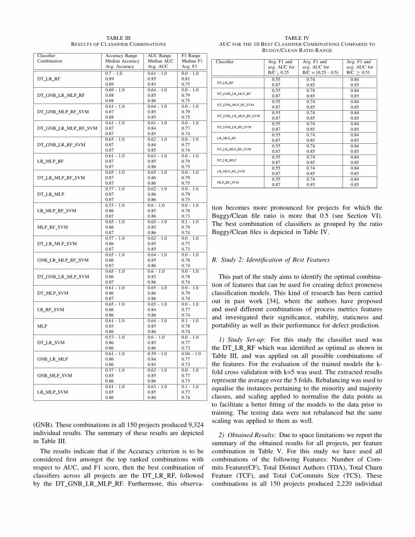
TABLE IIIRESULTS OF CLASSIFIER COMBINATIONS

Classifier Accuracy Range AUC Range F1 RangeCombination Median Accuracy Median AUC Median F1

Avg. Accuracy Avg. AUC Avg. F10.7 - 1.0 0.61 - 1.0 0.0 - 1.0

DT LR RF 0.89 0.85 0.810.89 0.85 0.750.69 - 1.0 0.64 - 1.0 0.0 - 1.0

DT GNB LR MLP RF 0.88 0.85 0.790.88 0.86 0.750.61 - 1.0 0.64 - 1.0 0.0 - 1.0

DT GNB MLP RF SVM 0.87 0.85 0.790.88 0.85 0.750.61 - 1.0 0.61 - 1.0 0.0 - 1.0

DT GNB LR MLP RF SVM 0.87 0.84 0.770.87 0.85 0.740.65 - 1.0 0.62 - 1.0 0.0 - 1.0

DT GNB LR RF SVM 0.87 0.84 0.770.87 0.85 0.740.61 - 1.0 0.63 - 1.0 0.0 - 1.0

LR MLP RF 0.87 0.85 0.790.87 0.86 0.750.65 - 1.0 0.65 - 1.0 0.0 - 1.0

DT LR MLP RF SVM 0.87 0.86 0.790.87 0.86 0.750.57 - 1.0 0.62 - 1.0 0.0 - 1.0

DT LR MLP 0.87 0.86 0.790.87 0.86 0.750.53 - 1.0 0.6 - 1.0 0.0 - 1.0

LR MLP RF SVM 0.86 0.85 0.780.87 0.86 0.730.65 - 1.0 0.65 - 1.0 0.1 - 1.0

MLP RF SVM 0.86 0.85 0.790.87 0.86 0.740.57 - 1.0 0.62 - 1.0 0.0 - 1.0

DT LR MLP SVM 0.86 0.85 0.770.87 0.85 0.730.65 - 1.0 0.64 - 1.0 0.0 - 1.0

GNB LR MLP RF SVM 0.86 0.85 0.780.87 0.86 0.740.65 - 1.0 0.6 - 1.0 0.0 - 1.0

DT GNB LR MLP SVM 0.86 0.85 0.780.87 0.86 0.740.61 - 1.0 0.65 - 1.0 0.0 - 1.0

DT MLP SVM 0.86 0.86 0.790.87 0.86 0.740.65 - 1.0 0.65 - 1.0 0.0 - 1.0

LR RF SVM 0.86 0.84 0.770.86 0.86 0.740.61 - 1.0 0.64 - 1.0 0.1 - 1.0

MLP 0.85 0.85 0.780.86 0.86 0.740.53 - 1.0 0.6 - 1.0 0.0 - 1.0

DT LR SVM 0.86 0.85 0.770.86 0.86 0.730.61 - 1.0 0.59 - 1.0 0.04 - 1.0

GNB LR MLP 0.86 0.84 0.770.86 0.85 0.730.57 - 1.0 0.63 - 1.0 0.0 - 1.0

GNB MLP SVM 0.85 0.85 0.770.86 0.86 0.730.61 - 1.0 0.63 - 1.0 0.1 - 1.0

LR MLP SVM 0.85 0.85 0.770.86 0.86 0.74

(GNB). These combinations in all 150 projects produced 9,324individual results. The summary of these results are depictedin Table III.

The results indicate that if the Accuracy criterion is to beconsidered first amongst the top ranked combinations withrespect to AUC, and F1 score, then the best combination ofclassifiers across all projects are the DT LR RF, followedby the DT GNB LR MLP RF. Furthermore, this observa-

TABLE IVAUC FOR THE 10 BEST CLASSIFIER COMBINATIONS COMPARED TO

BUGGY/CLEAN RATIO RANGE

Classifier Avg. F1 and Avg. F1 and Avg. F1 andavg. AUC for avg. AUC for avg. AUC forB/C ¡ 0.25 B/C = [0.25 - 0.5) B/C ≥ 0.51

DT LR RF0.550.87

0.740.85

0.840.85

DT GNB LR MLP RF0.550.87

0.740.85

0.840.85

DT GNB MLP RF SVM0.550.87

0.740.85

0.840.85

DT GNB LR MLP RF SVM0.550.87

0.740.85

0.840.85

DT GNB LR RF SVM0.550.87

0.740.85

0.840.85

LR MLP RF0.550.87

0.740.85

0.840.85

DT LR MLP RF SVM0.550.87

0.740.85

0.840.85

DT LR MLP0.550.87

0.740.85

0.840.85

LR MLP RF SVM0.550.87

0.740.85

0.840.85

MLP RF SVM0.550.87

0.740.85

0.840.85

tion becomes more pronounced for projects for which theBuggy/Clean file ratio is more that 0.5 (see Section VI).The best combination of classifiers as grouped by the ratioBuggy/Clean files is depicted in Table IV.

B. Study 2: Identification of Best Features

This part of the study aims to identify the optimal combina-tion of features that can be used for creating defect pronenessclassification models. This kind of research has been carriedout in past work [34], where the authors have proposedand used different combinations of process metrics featuresand investigated their significance, stability, staticness andportability as well as their performance for defect prediction.

1) Study Set-up: For this study the classifier used wasthe DT LR RF which was identified as optimal as shown inTable III, and was applied on all possible combinations ofthe features. For the evaluation of the trained models the k-fold cross validation with k=5 was used. The extracted resultsrepresent the average over the 5 folds. Rebalancing was used toequalise the instances pertaining to the minority and majorityclasses, and scaling applied to normalise the data points asto facilitate a better fitting of the models to the data prior totraining. The testing data were not rebalanced but the samescaling was applied to them as well.

2) Obtained Results: Due to space limitations we report thesummary of the obtained results for all projects, per featurecombination in Table V. For this study we have used allcombinations of the following Features: Number of Com-mits Feature(CF), Total Distinct Authors (TDA), Total ChurnFeature (TCF), and Total CoCommits Size (TCS). Thesecombinations in all 150 projects produced 2,220 individual

TABLE VRESULTS OF FEATURE COMBINATIONS

Feature a. Accuracy Range a. AUC Range a. F1 rangeCombination b.Median Accuracy b. Median AUC b. Median F1

c. Average Accuracy c. Average AIC c. Average F10.68 - 1.0 0.58 - 1.0 0.0 - 1.0

CF TCF TCS TDA 0.89 0.86 0.80.89 0.86 0.760.7 - 1.0 0.55 - 1.0 0.0 - 1.0

CF TCF TCS 0.89 0.85 0.810.89 0.85 0.750.63 - 1.0 0.59 - 1.0 0.0 - 1.0

CF TCS TDA 0.88 0.85 0.80.88 0.85 0.760.66 - 1.0 0.6 - 1.0 0.0 - 1.0

CF TCS 0.88 0.85 0.810.88 0.85 0.760.72 - 1.0 0.64 - 1.0 0.0 - 1.0

TCF TCS TDA 0.88 0.84 0.80.88 0.84 0.750.7 - 1.0 0.55 - 1.0 0.0 - 1.0

TCF TCS 0.87 0.82 0.780.87 0.83 0.730.6 - 1.0 0.46 - 1.0 0.0 - 1.0

TCS TDA 0.88 0.83 0.790.87 0.84 0.740.73 - 1.0 0.6 - 1.0 0.0 - 1.0

CF TCF TDA 0.86 0.83 0.780.87 0.83 0.720.62 - 1.0 0.5 - 1.0 0.0 - 1.0

CF TCF 0.85 0.81 0.760.86 0.82 0.710.69 - 1.0 0.61 - 1.0 0.0 - 1.0

TCF TDA 0.85 0.8 0.750.85 0.81 0.70.5 - 1.0 0.6 - 1.0 0.13 - 1.0

CF TDA 0.84 0.81 0.770.85 0.82 0.710.33 - 1.0 0.4 - 1.0 0.13 - 1.0

CF 0.82 0.8 0.750.84 0.81 0.690.47 - 1.0 0.44 - 1.0 0.0 - 1.0

TCS 0.84 0.79 0.710.83 0.79 0.670.63 - 1.0 0.5 - 1.0 0.0 - 1.0

TCF 0.82 0.76 0.690.83 0.77 0.650.39 - 1.0 0.4 - 1.0 0.07 - 1.0

TDA 0.8 0.81 0.730.81 0.81 0.68

results. The full results list can be found on the data repositoryaccompanying this paper [23].

C. Study 3: Comparison of Process and Source Code Metrics

This study aims at performing a comparison between theefficiency of using Source Code Metrics versus using ProcessMetrics for carrying out Fault-Proneness prediction. It iscarried out on a subset of data made available for softwareengineering research as part of the PROMISE repository [33].

1) Study Set-up: All combinations of the available clas-sifiers were used for this experiment and the Feature com-bination used was the one identified as optimal in SectionV-B. To select the subset of systems on which to conduct thisstudy we manually investigated the contents of the PROMISErepository to identify projects for which a valid Git repositoryis still available. Given the age of the repository and it’sspecific structure this process yielded only 11 systems for

which process metrics could be mined. For these 11 systemsthe data between the PROMISE dataset and our system werereconciled. The reconciliation process consisted of only usingdata pertaining to files present both in data extracted from Gitrepositories and in the PROMISE dataset. In addition, the fileshad to be active with at least a single commit in the latest 30%of the total commits of the system. The files’ classes were setfrom the manually curated PROMISE dataset. The processused afterwards is the same as in Sections V-A and V-B.The data were rebalanced in both cases and independentlyscaled. The process presented so far was designed to giveboth approaches an equal ammount of data and to be easilyreplicated by other researchers. The evaluation of the modelswas implemented using k-fold cross validation where k=5 foreach of the approaches, Source-Code Metrics and ProcessMetrics respectively, and the presented results depict theaverage over all 5-folds of this evaluation.

2) Obtained Results: Due to space limitations, we reporthere the highlights of the obtained results. The full resultslist can be found on the data repository accompanying thispaper [23]. For this study a voting classifier was utilised usingall combinations of the following classifiers: Decision Trees(DT), Random Forests (RF), Linear Regression (LR), Multi-Layer Perceptron (MLP), Support Vector Machines(SVM),and Gaussian Naive Bayes(GNB). The Features used were:Number of Commits Feature(CF), Total Distinct Authors(TDA), Total Churn (TC), and Total CoCommitsSize Feature(TCS) for extracting process metrics and all features availablewere used from the PROMISE dataset. This process wasapplied on 11 projects and yielded a total of 756 results foreach metric type. The results are shown in Table VI.

D. Study 4: Cross Project ValidationFor this study, we have trained the classifiers in a collection

of projects (training set) and we have applied them to anotherset projects (testing set) for comparing the obtained resultswith the ones obtained when the classifiers are trained andapplied only in one project.

1) Study Set-up: For this study the optimal classifier iden-tified in Section V-A and the optimal feature combinationidentified in Section V-B were used. To prepare the data wefiltered the available systems selecting only those having lessthan 20K and more than 250 files and then split these into threeperformance classes using the ratio of fault-prone over healthyfiles in the system. This yielded a total of 26 projects with aB/C ratio in the interval [0, 0.25), 20 projects with a ratio inthe interval [0.25, 0.5) and 44 projects with a B/C ratio ≥0.5 (see also Table IV). These groups were then divided intotwo randomly selected groups, and one group was used fortraining a model while the other group was used for evaluation.Given the uneven size of the different systems it was necessaryto upsample the data available for each one of them so asto have all projects represented approximately equally in thetraining set and avoiding it being dominated by the largestsystems. Rebalancing of the minority and majority classes was

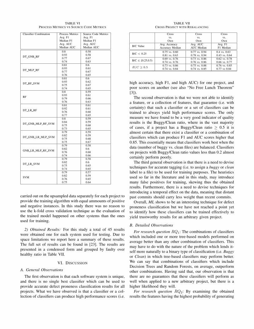
TABLE VIPROCESS METRICS VS SOURCE CODE METRICS

Classifier Combination Process Metrics Source Code MetricsAvg. F1 Avg. F1Median F1 Median F1Avg. AUC Avg. AUCMedian AUC Median AUC

DT GNB RF

0.80.930.770.74

0.580.580.670.63

DT MLP RF

0.810.930.770.76

0.60.610.670.65

DT RF SVM

0.810.930.750.74

0.60.620.670.65

RF

0.80.930.790.76

0.590.610.660.63

DT LR RF

0.810.920.760.77

0.610.610.680.65

DT GNB MLP RF SVM

0.80.840.750.73

0.590.590.680.65

DT GNB LR MLP SVM

0.790.820.750.75

0.590.590.680.67

GNB LR MLP RF SVM

0.790.820.760.74

0.580.60.680.66

DT LR SVM

0.790.820.750.74

0.580.60.650.65

SVM

0.790.820.760.75

0.570.590.650.64

carried out on the upsampled data separately for each project toprovide the training algorithm with equal ammounts of positiveand negative instances. In this study there was no reason touse the k-fold cross validation technique as the evaluation ofthe trained model happened on other systems than the onesused for training.

2) Obtained Results: For this study a total of 45 resultswere obtained one for each system used for testing. Due tospace limitations we report here a summary of these results.The full set of results can be found in [23]. The results arepresented in a condensed form and grouped by faulty overhealthy ratio in Table VII.

VI. DISCUSSION

A. General Observations

The first observation is that each software system is unique,and there is no single best classifier which can be used toprovide accurate defect proneness classification results for allprojects. What we have observed is that a classifier or a col-lection of classifiers can produce high performance scores (i.e.

TABLE VIICROSS PROJECT WITH REBALANCING

Cross Cross Crossvs. vs. vs.

Own Own Own

B/C Value Avg. AccuracyAccuracy Median

Avg. AUCAUC Median

Avg. F1F1 Median

B/C < 0.25 0.75 vs. 0.600.81 vs. 0.63

0.77 vs. 0.940.78 vs. 0.94

0.4 vs. 0.630.43 vs. 0.64

B/C ∈ [0.25,0.5) 0.69 vs. 0.760.74 vs. 0.76

0.73 vs. 0.860.76 vs. 0.86

0.62 vs. 0.780.66 vs. 0.77

B/C ≥ 0.50.73 vs. 0.860.74 vs. 0.84

0.75 vs. 0.880.74 vs. 0.85

0.76 vs. 0.850.77 vs 0.84

high accuracy, high F1, and high AUC) for one project, andpoor scores on another (see also “No Free Lunch Theorem”[3]).

The second observation is that we were not able to identifya feature, or a collection of features, that guarantee (i.e. withcertainty) that such a classifier or a set of classifiers can betrained to always yield high performance scores. The onlymeasure we have found to be a very good indicator of qualityresults is the Buggy/Clean ratio, where in the vast majorityof cases, if a project has a Buggy/Clean ratio ≥ 0.5 it isalmost certain that there exist a classifier or a combination ofclassifiers which can produce F1 and AUC scores higher that0.85. This essentially means that classifiers work best when thedata (number of buggy vs. clean files) are balanced. Classifierson projects with Buggy/Clean ratio values less than 0.2 almostcertainly perform poorly.

The third general observation is that there is a need to devisetechniques for accurate tagging (i.e. to assign a buggy or cleanlabel to a file) to be used for training purposes. The heuristicsused so far in the literature and in this study, may introducemany false positives for training, skewing thus the obtainedresults. Furthermore, there is a need to devise techniques forintroducing a temporal effect on the data, meaning that distantpast commits should carry less weight than recent commits.

Overall, ML shows to be an interesting technique for defectproneness classification but we have not reached a point yetto identify how these classifiers can be trained effectively toyield trustworthy results for an arbitrary given project.

B. Detailed Observations

For research question RQ1: The combinations of classifierswhich included one or more tree-based models performed onaverage better than any other combination of classifiers. Thismay have to do with the nature of the problem which lends it-self more naturally to a binary type of classification (i.e. Buggyor Clean) in which tree-based classifiers may perform better.We can say that combinations of classifiers which includeDecision Trees and Random Forests, on average, outperformother combinations. Having said that, our observation is thatthere are no guarantees that these classifiers will perform aswell when applied to a new arbitrary project, but there is ahigher likelihood they will.

For research question RQ2: By examining the obtainedresults the features having the highest probability of generating

high quality results is the combination of all four features,followed by the combination of CF (number of commits) andTCS (total co-commit size) and TCF (total churn). However,looking at the minimal set of features which can be used andstill produce high quality results is any combination of twoof CF (number of commits) and TCS (total co-commit size)and TCF (total churn). Another observation is that the TDA(total distinct authors) feature on its own does not provide highquality results, but only when combined with other features.

For research question RQ3: Here we can say that processmetrics seem to outperform the source code metrics for defect-proneness classification purposes. This is an encouragingobservation as process metrics are language agnostic and theircompilation does not require specialised parsers and metricsextractors. This result was anticipated, as software metrics maymore often exhibit a variability in values over the differentcommits while the files maintain their tag value (i.e. Buggy orClean), and vice versa, that is metrics may more often exhibit avariability in values over the different commits while the fileschange their tag value. This property may generate conflictingdata for the classifier. In contrast, process metrics may exhibita variability too, but maintain a better type of “history” featurevalues as the project evolves.

For research question RQ4: Here our observation is thatcross project classifier training and application does not yieldhigh quality results. When classifiers are trained in someprojects and applied to other projects the classification resultsare not as accurate as when the classifier is applied to the sameproject as the one it is trained on. This may be explained fromthe fact that the profiles of process metric values are kind ofproject specific as they depict the history of the project and theactivity on each file. This is an interesting result, as it disputesthe case of one trained model fits all.

C. Threats to Validity

We identify three threats. The first threat has to do with theway tagging is performed in order to create a training set. Forour study we consider for tagging purposes the most recent30% of the commits, while we maintain historical informationfrom the past 70% of commits. For the feature value vectorsof the distant past 70% of the commits we are either providinga DC value or no value (e.g. see Section IV-C). This createsthe potential for false positives to be generated during tagging.The second threat has to do with how files are tagged withina single commit. For this study, if a file participates on a bugfixing commit then we consider all files in the commit asbuggy. This is an overestimate and introduces the possibilityof false positives. The most accurate approach would be tobe able to tag all files in all commits in the history of theproject with their correct label. However, this would be almostimpossible for such large projects we have considered in thecourse of this study. It would be though a valid approach fornew projects, where accurate labeling can commence on earlystages of the project. The third threat has to do with the usedfeatures. Since the purpose of the study was to provide resultsfrom a large data set and not to propose new features, we

have considered features which are commonly used in theresearch literature. There may be other features which relate toprocess metrics and which the community has not consideredyet, which may produce good defect proneness classificationresults. This can also be considered an open problem forfurther investigation.

VII. CONCLUSION

This paper reports on the results of a set of experimentsconducted in order to evaluate the use of Machine Learningfor defect proneness classification. Over the past few years wehave seen a tremendous growth on research and publicationsrelated to Machine Learning for software maintenance, andin particular for defect proneness classification and defectprediction. Even though there is a significant body of workconducted on evaluating Machine Learning techniques fordefect proneness classification, the significance of this paper isthat it is the first work to our knowledge that examines such alarge corpus of open source data aiming to concretely addressfour key research questions which relate to experimentallyidentifying the best classifiers, the best features, whetherprocess metrics outperform software metrics as predictors, andwhether cross project training and application can be a viableoption with respect to the quality of the obtained results. Theexperiments conducted revealed a number of observations.First, Machine Learning techniques are not guaranteed toperform well in all projects. Each software project has aspecific life-cycle and “personality” profile of its own, and“a one classifier fits all” approach is not feasible. Second, wehave seen that Machine Learning techniques are more likely toperform well when the buggy/clean ratio of the system filesis between 0.5 and 2. Note that a ratio of 1 indicates thatthere are as many buggy files and clean files. Third, therewas a clear indication that process metrics perform betteror, in some cases, at least as well as software metrics. Thisimplies that there is a strong indication that process relatedmetrics can safely be used as predictors. Fourth, training theclassifiers in one set of systems and applying on another isnot a good approach, as the best classification results areobtained when the classifier is applied on the same system it istrained on. Overall, ML for defect proneness classification is apromising area of work that still has a number open problemsto investigate. These include identifying new features to useas predictors, creating better tagging tools, and combining MLwith static and dynamic analysis to increase the performanceof the classifiers.

REFERENCES

[1] Github, Build software better, together - https://github.com.[2] Guillaume Lemaı̂tre, Fernando Nogueira, and Christos K Aridas. 2017.

Imbalanced-learn: A python toolbox to tackle the curse of imbalanceddatasets in machine learning. The Journal of Machine Learning Research18, 1 (2017), 559–563.

[3] Wolpert D.H., Macready W.G. . “No Free Lunch Theorems for Opti-mization” . IEEE Transactions on Evolutionary Computation, Vol. 1, pp.67-82, 1997.

[4] Taghi M Khoshgoftaar and Naeem Seliya. 2002. Tree-based softwarequality estimation models for fault prediction. In Software Metrics, 2002.Proceedings. Eighth IEEE Symposium on. IEEE, 203–214.

[5] Shuo Wang and Xin Yao. 2013. Using class imbalance learning forsoftware defect prediction. IEEE Transactions on Reliability 62, 2(2013), 434–443.

[6] David Gray, et. al, 2009. Using the support vector machine as aclassification method for software defect prediction with static codemetrics. In International Conference on Engineering Applications ofNeural Networks. Springer, 223–234.

[7] Burak Turhan and Ayse Bener. 2009. Analysis of Naive Bayes’assumptions on software fault data: An empirical study. Data &Knowledge Engineering 68, 2 (2009), 278–290.

[8] Mie Mie Thet Thwin and Tong-Seng Quah. 2005. Application of neuralnetworks for software quality prediction using object-oriented metrics.Journal of systems and software 76, 2 (2005), 147–156.

[9] Cagatay Catal and Banu Diri. 2009a. Investigating the effect of datasetsize, metrics sets, and feature selection techniques on software faultprediction problem. Information Sciences 179, 8 (2009), 1040–1058.

[10] Venkata Udaya B Challagulla, Farokh B Bastani, I-Ling Yen, andRaymond A Paul. 2008. Empirical assessment of machine learning basedsoftware defect prediction techniques. International Journal on ArtificialIntelligence Tools 17, 02 (2008), 389–400.

[11] Tim Menzies, Jeremy Greenwald, and Art Frank. 2007. Data miningstatic code attributes to learn defect predictors. IEEE Trans. on SoftwareEngineering 1 (2007), 2–13.

[12] Jun Zheng. 2010. Cost-sensitive boosting neural networks for softwaredefect prediction. Expert Systems with Applications 37, 6 (2010), 4537–4543.

[13] Ahmed E Hassan. 2009. Predicting faults using the complexity of codechanges. In Proceedings of the 31st Intl. Conf. on Software Engineering.IEEE Comp. Society, 78–88.

[14] Nachiappan Nagappan, Thomas Ball, and Andreas Zeller. 2006. Miningmetrics to predict component failures. In Proceedings of the 28thinternational conference on Software engineering. ACM, 452–461.

[15] Thomas Zimmermann, Nachiappan Nagappan, Harald Gall, EmanuelGiger, and Brendan Murphy. 2009. Cross-project defect prediction: alarge scale experiment on data vs. domain vs. process. In Proceedingsof the the 7th joint meeting of the European software engineeringconference and the ACM SIGSOFT symposium on The foundations ofsoftware engineering. ACM, 91–100.

[16] Ahmet Okutan and Olcay Taner Yıldız. 2014. Software defect predictionusing Bayesian networks. Empirical Software Engineering 19, 1 (2014),154–181.

[17] Peng He, Bing Li, Xiao Liu, Jun Chen, and Yutao Ma. 2015. Anempirical study on software defect prediction with a simplified metricset. Information and Software Technology 59 (2015), 170–190.

[18] T. T. Wong, “Performance evaluation of classification algorithms byk-fold and leave-one-out cross validation”, Pattern Recognition, 48(9):pp.2839-2846, 2015.

[19] Shyam R. Chidamber and Chris F. Kemerer, “A metrics suite for objectoriented design”. IEEE Trans. Software Eng., 20(6):476 pp. 493, 1994.

[20] V. R. Basili, L. C. Briand, and W. L. Melo, “A Validation of Objectoriented Design Metrics as Quality Indicators,” Trans. on Software Eng., 22(10):pp. 751 - 761, 1996.

[21] D. Romano, M. Pinzger, “Using Source Code Metrics to Predict Change-Prone Java Interfaces”, 27th International Conference on SoftwareMaintenance, 2011.

[22] F. Toure, M. Badri, L. Lamontagne, “Predicting different levels of theunit testing effort of classes using source code metrics: a multiple casestudy on open-source software”, Innovations in Systems and SoftwareEngineering 14, pp. 15-46, 2018.

[23] https://figshare.com/s/b3741f9d0c3a939669db[24] F. Zhang, F. Khomh, Y. Zou and A. E. Hassan, “An Empirical Study on

Factors Impacting Bug Fixing Time,” 2012 19th Working Conferenceon Reverse Engineering, pp. 225-234, 2012.

[25] Menzies, T., Milton, Z., Turhan, B. et al. “Defect prediction from staticcode features: current results, limitations, new approaches”. AutomatedSoftware Eng. 17, pp. 375–407, 2010.

[26] Z. Toth, P. Gyimesiand R. Ferenc. “A Public Bug Database of GitHubProjects and Its Application in Bug Prediction”. Springer, Intern.Conf.on Computational Sciences and Its Applications pp. 625 - 638, 2016.

[27] A. Tornhill. “Your code as a crime scene: use forensic techniques toarrest defects, bottlenecks, and bad design in your programs.” PragmaticBookshelf, 2015.

[28] C. Tantithamthavorn, S. McIntosh, A. E. Hassan, K. Matsumoto. “TheImpact of Automated Parameter Optimization on Defect PredictionModels”. IEEE Trans. Software Eng., 45(7):pp. 683 - 711, 2018.

[29] C. Tantithamthavorn, A. E. Hassan, K. Matsumoto. “The Impact ofClass Rebalancing Techniques on the Performance and Interpreta-tion of Defect Prediction Models”. IEEE Trans. Software Eng., DOI10.1109/TSE.2018.2876537, IEEE, 2018.

[30] M. Kondo, C.P. Bezemer, Y. Kamei, A. E. Hassan, and O. Mizuno. “TheImpact of feature reduction techniques on defect prediction models.”Empirical Software Engineering 24:pp. 1925 - 1963, 2019.

[31] J. Jiarpakdee, C. Tantithamthavorn, A. E. Hassan. “The Impact of Corre-lated Metrics on the Interpretation of Defect Prediction Models.” IEEETrans. Software Eng. early access, DOI 10.1109/TSE.2019.2891758,2019.

[32] Y. Kamei, E. Shihab, B. Adams, A.E. Hassan, A. Mockus, A. Sinha,N. Ubayashi, “A large-scale empirical study of just-in-time qualityassurance”, IEEE Trans. Software Eng., 39 (6): pp. 757-773, 2013.

[33] J. Sayyad Shirabad and T.J. Menzies, “The PROMISE Repository ofSoftware Engineering Databases”, 2005.

[34] F. Rahman, P. Devanbu, “How, and Why, Process Metrics are Better,” inProceedings of the International Conference on Software Engineering,2013, pp. 432 – 441.

[35] S. Lessmann, B. Baesens, C. Mues, and S. Pietsch, “BenchmarkingClassification Models for Software Defect Prediction: A ProposedFramework and Novel Findings”. Trans. Software Eng., 34(4): pp. 485- 496, 2008.

[36] T. Hall, S. Beecham, D. Bowes, D. Gray, and S. Counsell, “A Sys-tematic Literature Review on Fault Prediction Performance in SoftwareEngineering”, IEEE Trans. on Software Eng., 38(6): pp. 1276 – 1304,2012.

[37] M. D’Ambros, M. Lanza, and R. Robbes, “Evaluating defect predictionapproaches: a benchmark and an extensive comparison”. EmpiricalSoftware Eng. 17, pp. 531–577, 2012.

[38] C. Tantithamthavorn and A. E. Hassan, “An Experience Report onDefect Modelling in Practice: Pitfalls and Challenges”. in Proceedingsof the International Conference on Software Engineering: SoftwareEngineering in Practice Track (ICSE-SEIP), pp. 286 – 295, 2018.

[39] L. Pascarella, F. Palomba, A. Bacchelli, “Fine-grained just-in-time defectprediction”, Journal of Systems and Software 150: pp.22-36, 2018.

[40] C. Tantithamthavorn, S. McIntosh, A. E. Hassan, K. Matsumoto, “TheImpact of Automated Parameter Optimization on Defect PredictionModels”. IEEE Trans. on Software Eng. 45(7): pp. 683 - 711, 2019.