report on compliance with mcs installation standards v32
TRANSCRIPT
Analysis of Heat Pump data from the Renewable Heat Premium Payment Scheme (RHPP) to the Department of Business, Energy and Industrial Strategy: Compliance with MCS Installation Standards. Issued: February 2017 RAPID-HPC authors: Colin Gleeson, Phillip Biddulph, Robert Lowe, Jenny Love, Alex Summerfield, Eleni Oikonomou, Jez Wingfield & Chris Martin
UK Data Archive Study Number 8151 - Renewable Heat Premium Payment Scheme: Heat Pump Monitoring: Cleaned Data, 2013-2015

1
Confidentiality, copyright & reproduction:
This report is the copyright of RAPID-HPC, prepared under contract to BEIS. The contents of this
report may not be reproduced in whole or in part, without acknowledgement. BEIS and RAPID-HPC
accept no liability whatsoever to any third party for any loss or damage arising from any interpretation or
use of the information contained in this report, or reliance on any views expressed herein.
©RAPID-HPC 2017.

2
Table of contents
Executive Summary .................................................................................................................................. 10
Report on compliance with MCS installation standards .............................................................. 14 1
Introduction ............................................................................................................................................................................... 14
Substantive MIS 3005 changes ............................................................................................................................................... 16
Installer qualifications and handover ..................................................................................................................................... 18
Number of heat pumps, manufacturers and models .......................................................................................................... 18
System boundaries and monitored data ................................................................................................................................ 19
Heat pump sizing; have installers complied with MCS standards? ............................................ 20 2
Introduction ............................................................................................................................................................................... 20
Heat loss calculations ............................................................................................................................................................... 20
Radiator sizing ........................................................................................................................................................................... 22
Heat pump sizing, compliance with MCS ............................................................................................................................ 24
Peak load and Plant size ratio ................................................................................................................................................. 26
Net capacity ................................................................................................................................................................................ 30
Load Factor ................................................................................................................................................................................ 34
Ground loop design .................................................................................................................................................................. 36
Conclusions ................................................................................................................................................................................ 39
How do actual space and water heating demand compare to the estimated figures on the 3
MCS certificate and on the EPC? ........................................................................................................... 41
Introduction ............................................................................................................................................................................... 41
RHPP annual energy assessment ............................................................................................................................................ 42
EPC annual energy assessment ............................................................................................................................................... 45
Conclusion .................................................................................................................................................................................. 49
Do systems sterilise the hot water tank for legionella control? If so, how often? ................... 51 4
Sterilisation ................................................................................................................................................................................. 51
Analysis methodology .............................................................................................................................................................. 53
Analysis results ........................................................................................................................................................................... 54
Conclusion .................................................................................................................................................................................. 55
What are the actual flow temperatures at the MCS 3005 design temperature conditions? 5
What Heat Emitter Guide star rating would apply, based on the actual flow temperatures? ....... 56
Introduction ............................................................................................................................................................................... 56
Maximum temperature assessment ........................................................................................................................................ 57
Weather compensation ............................................................................................................................................................. 60
Conclusions ................................................................................................................................................................................ 60

3
How do the measured SPFs for space heating compare with SPFs from the Heat Emitter 6
Guide? ......................................................................................................................................................... 62
Introduction ............................................................................................................................................................................... 62
Derived maximum flow temperatures ................................................................................................................................... 63
Modelling of SPF as a function of load factor ..................................................................................................................... 66
Conclusion .................................................................................................................................................................................. 66
References .................................................................................................................................................. 68
Appendix A ......................................................................................................................................... 71 7
System boundaries and monitored data parameters ........................................................................................................... 71
Appendix B ......................................................................................................................................... 74 8
Weather compensation curves ................................................................................................................................................ 74
Appendix C ......................................................................................................................................... 76 9
Heat pump net capacity ........................................................................................................................................................... 76
ASHP net capacity corrections ............................................................................................................................................... 78
ASHP fixed speed ..................................................................................................................................................................... 78
ASHP variable speed ................................................................................................................................................................ 78
Ground Source Heat Pump fixed speed ............................................................................................................................... 79
Conclusions ................................................................................................................................................................................ 80
Appendix D ...................................................................................................................................... 81 10
Potential impact of low Load Factor ..................................................................................................................................... 81
Figures
Figure 1-1 RHPP quote, installation and commission dates and dates of MCS standards ............................ 15
Figure 1-2 SPF, flow temperature and star rating (HEG, 2011) ........................................................................ 17
Figure 2-1 Example radiator catalogue ................................................................................................................... 23
Figure 2-2 Manufacturer’s ASHP capacity as a function of outdoor air temperature for 6 kW nominal
output ........................................................................................................................................................................... 30
Figure 2-3 Assessment of peak heat power versus installer net capacity (kW). ............................................... 32
Figure 2-4 Assessment of peak heat power versus installer net capacity (kW) showing HPs with >10%
boost............................................................................................................................................................................. 32
Figure 2-5 Load factor for all heat pumps ............................................................................................................. 35
Figure 2-6 Load factors ASHPs ............................................................................................................................... 35
4
Figure 2-7 Load factors GSHPs .............................................................................................................................. 36
Figure 2-8 “Rated” ground loop circulating pump power as a percentage of heat pump power ................. 38
Figure 2-9 Example evaporator pressure drop at design brine flow rate in the ground loop (for GSHPs)
....................................................................................................................................................................................... 39
Figure 3-1 Installers’ estimate of annual heat demand versus actual heat generated for all heat pumps ... 43
Figure 3-2 Installers’ estimate of annual heat demand versus actual heat demand - GSHPs ........................ 44
Figure 3-3 Installers’ estimate of annual heat demand versus actual annual heat demand ASHPs .............. 44
Figure 3-4 Difference between MCS predicted and actual heat energy for ASHPs and GSHPs ................. 44
Figure 3-5 EPC predicted annual space heating demand versus measured for all heat pumps .................... 46
Figure 3-6 EPC predicted annual DHW heat demand versus measured for all heat pumps ........................ 46
Figure 3-7 EPC predicted ASHP annual space heating heat demand versus measured ................................ 47
Figure 3-8 EPC predicted GSHP annual space heating heat demand versus measured ................................ 47
Figure 3-9 EPC and MCS predicted total heat demand versus actual (same sites joined). ............................ 48
Figure 3-10 EPC and MCS predicted ASHP total heat demand versus actual (same sites joined) .............. 48
Figure 3-11 EPC and MCS predicted GSHP total heat demand versus actual (same sites joined) .............. 49
Figure 4-1 Separate DHW cylinder with metered domestic hot water immersion ......................................... 52
Figure 4-2 Assessment of apparent immersion frequency .................................................................................. 54
Figure 5-1 Derived peak flow temperature for all heat pumps and all emitters .............................................. 58
Figure 5-2 Star temperature versus derived peak flow temperature .................................................................. 59
Figure 5-3 Derived peak flow temperatures for all heat pumps with radiators ............................................... 59
Figure 5-4 Derived peak flow temperatures for all heat pumps with underfloor heating ............................. 60
Figure 6-1 Derived peak flow temperatures for GSHPs ..................................................................................... 63
Figure 6-2 GSHP SPFH2 versus HEG SPF ........................................................................................................... 64
Figure 6-3 Derived peak flow temperatures for ASHPs ..................................................................................... 65
Figure 6-4 ASHP RHPP SPFH2 versus HEG SPF ............................................................................................... 65

5
Figure 7-1 SEPEMO system boundaries (derived from Riviere et al., 2011) with the addition of H5
boundary that accounts for heat losses from the hot water cylinder................................................................. 71
Figure 7-2 An example simplified schematic of the metering arrangement for a monobloc ASHP that
provides heat to space heating and a domestic hot water cylinder with an immersion element................... 73
Figure 7-3 An example of a GSHP with an integrated domestic hot water cylinder. ..................................... 73
Figure 8-1 Weather compensation curves.............................................................................................................. 75
Figure 10-1 Envelope of monthly COPs versus monthly load factors. The upper bound includes
continuous parasitic electrical loads. The lower bound includes a 200 W continuous parasitic electrical
load. .............................................................................................................................................................................. 81
Figure 10-2 Measured SPF as a function of Load Factor for all heat pumps .................................................. 82
Figure 10-3 Monthly COP and load factors for ASHPs ..................................................................................... 83
Figure 10-4 Monthly COP and load factors for GSHPs ..................................................................................... 84
Tables
Table 1–1 MCS heat pump installation standards in place during the RHPP programme............................ 14
Table 2–1 Typical panel radiator output correction factors ................................................................................ 23
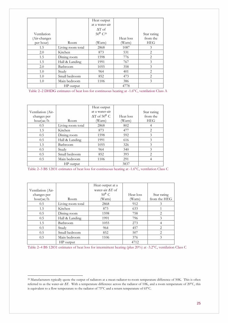
Table 2–2 DHDG estimates of heat loss for continuous heating at -1.6C, ventilation Class A ................. 25
Table 2–3 BS 12831 estimates of heat loss for continuous heating at -1.6C, ventilation Class C .............. 25
Table 2–4 BS 12831 estimates of heat loss for intermittent heating (plus 20%) at -3.2C, ventilation Class
C .................................................................................................................................................................................... 25
Table 2–5 BS 12831 estimates of heat loss for intermittent heating (plus 20%) at -3.2C, ventilation Class
C with throat restrictor chimneys in living and dining rooms (highlighted in red) ......................................... 26
Table 2–6 GSHP Manufacturer’s capacity data sheet .......................................................................................... 28
Table 2–7 GSHP capacity derived from manufacturer’s graphical data ........................................................... 28
Table 2–8 ASHP peak capacity values at different sink and source temperatures for a nominal 6 kW heat
pump ............................................................................................................................................................................ 29

6
Table 2–9 ASHP ‘integrated capacity values’ at different sink and source temperatures for a nominal for 6
kW heat pump ............................................................................................................................................................ 29
Table 2–10 Ground loop metadata provided by installers .................................................................................. 37
Table 6–1 Statistical analysis of measured and HEG SPF .................................................................................. 66
Table 7–1 The complete set of parameters included in the monitored data .................................................... 72
Table 8–1 Weather compensation derived return temperatures ........................................................................ 74
Table 9–1 ASHP EN 14511 test regime ................................................................................................................ 77
Table 9–2 GSHP EN 14511 test regime ................................................................................................................ 77
Table 9–3 ASHP Fixed speed compressor corrections for -2C ....................................................................... 78
Table 9–4 ASHP variable speed compressor corrections for -2C ................................................................... 79
Table 9–5 GSHP Fixed speed compressor corrections for -2C ....................................................................... 79
7
Nomenclature
PERFORMANCE EFFICIENCY NOMENCLATURE
COP Heat pump (HP) coefficient of performance
SPFHn HP seasonal performance factor for heating at SEPEMO boundary Hn
MONITORED VARIABLES
Eb Electricity for whole system boost only Edhw Electricity for domestic hot water (typically an immersion heater) Ehp Electricity for the heat pump unit (may include a booster heater and circulation pump) Esp Electricity for boost to space heating only Fhp Flow rate of water from heat pump (may be space heating only) Fhw Flow rate of water to DHW cylinder (if separately monitored) Hhp Heat from heat pump (may be space heating only) Hhw Heat to DHW cylinder (if separately monitored) Tco Temperature of water leaving the condenser Tin For ASHP: Temperature of refrigerant leaving the evaporator
For GSHP: Temperature of ground loop water into the heat pump Tsf Flow temperature of water to space heating Twf Flow temperature of water to cylinder
(Note that external temperature, Tex, was not measured directly. Data from a publicly available database
were used in the analysis.)
RHPP ENERGY AND POWER UNITS
Energy J Joule SI unit of energy Energy kWh 3.6 MJ Customary unit of energy for residential energy use
Energy MWh, GWh 3.6 GJ, 3.6 TJ
Power W Watt, J/s SI unit of power and heat flow Power Wh/2 minutes 30 W Base unit of energy for monitored data in RHPP trial,
limit of resolution of power – note that power and heat have been recorded at 2 minute intervals
Power kWh/year 3.6 MJ/year Customary unit for rate of residential energy use. 1kWh/yr ≈ 0.11416 W
Power kW 1000 W Typical unit for measurement of heating system ratings
KEY ACRONYMS AND ABBREVIATIONS
BEIS Department of Business, Energy and Industrial Strategy
DECC Department of Energy and Climate Change
EST Energy Saving Trust Preliminary Assessment
Preliminary assessment of the RHPP data performed by DECC (Wickins, 2014)
RAPID-HPC Research and Analysis on Performance and Installation Data – Heat Pump Consortium
RHPP Renewable Heat Premium Payment Scheme
MCS Microgeneration Certification Scheme - a nationally recognised quality assurance scheme. MCS certifies microgeneration technologies used to produce electricity and heat from renewable sources.

8
MIS Microgeneration Installation Standards. MIS 3005 sets out requirements for MCS contractors undertaking the supply, design, installation, set to work, commissioning and handover of microgeneration heat pump systems.
SEPEMO SEasonal PErformance factor and MOnitoring
DHW Domestic Hot Water
DHDG Domestic Heating Design Guide
HEG Heat Emitter Guide
Likely SPF HEG values of SPF based on heat pump type and space heating flow temperature

9
Context
The RHPP policy provided subsidies for private householders, Registered Social Landlords and
communities to install renewable heat measures in residential properties. Eligible measures included air
and ground-source heat pumps, biomass boilers and solar thermal panels.
Around 14,000 heat pumps were installed via this scheme. BEIS funded a detailed monitoring campaign,
which covered 700 heat pumps (around 5% of the total). The aim of this monitoring campaign was to
provide data to enable an assessment of the efficiencies of the heat pumps and to gain greater insight into
their performance. The RHPP scheme was administered by the Energy Savings Trust (EST) who engaged
the Buildings Research Establishment (BRE) to run the meter installation and data collection phases of
the monitoring program. They collected data from 31 October 2013 to 31 March 2015.
RHPP heat pumps were installed between 2009 and 2014. Since the start of the RHPP Scheme, the
installation requirements set by MCS standards and processes have been updated.
BEIS contracted RAPID-HPC to analyse this data. The data provided to RAPID-HPC included physical
monitoring data, and metadata describing the features of the heat pump installations and the dwellings in
which they were installed.
The work of RAPID-HPC consisted of cleaning the data, selection of sites and data for analysis, analysis,
and the development of conclusions and interpretations. The monitoring data and contextual information
provided to RAPID-HPC are imperfect and the analyses presented in this report should be considered
with this in mind. Discussion of the data limitations is provided in the reports and is essential to the
conclusions and interpretations presented. This report does not assess the degree to which the heat
pumps assessed are representative of the general sample of domestic heat pumps in the UK. Therefore
these results should not be assumed to be representative of any sample of heat pumps other than that
described.
Acknowledgements
The authors gladly acknowledge the inputs to this report of Roger Nordman of SP Technical Research
Institute and Tom Garrigan of BSRIA. The work has been supported throughout by colleagues at BEIS,
particularly by Penny Dunbabin, Amy Salisbury and Jon Saltmarsh.

10
Executive Summary
The Microgeneration Certification Scheme Installation Standard (MCS MIS) 3005 provides the
‘requirements for contractors undertaking the supply, design, installation, set to work commissioning and
handover’ of microgeneration heat pump systems for compliance with the certification scheme.
The aim of this report was to use monitored data from sites enrolled in the Department of Energy &
Climate Change’s (DECC) Renewable Heat Premium Payment (RHPP) scheme to assess how well RHPP
Trial installations reflect the design requirements of MCS MIS 3005. In July 2016, the Department of
Energy & Climate Change was merged with the Department for Business, Innovation and Skills to create
the Department for Business, Energy & Industrial Strategy (BEIS). The appellation BEIS is applied where
appropriate to reflect that change.
The MCS MIS 3005 standard was changed several times during the period over which RHPP heat pumps
were designed and installed. Some of these changes were significant. In principle, systems should have
been designed to whichever version of the standard was mandatory at the time of quotation, not
installation. The metadata supplied with the RHPP data does not include the MIS 3005 version used for
the design and quotation dates are only provided for privately owned properties. It is therefore not
possible to determine with certainty which version of the standards was applied by the designer in each
case.
For these reasons, the assessment in this report cannot provide precise estimates of how many systems
complied with the standards. However, we examine eight elements of the MIS 3005 standard, namely:
Calculation of heat loss
Heat pump sizing
Radiator sizing
Calculation of measured annual energy use and comparison with the installers’ estimates and
EPC calculations
Sterilisation of domestic hot water
Specification of flow temperature at design conditions.
Weather compensation
Actual measured SPFH2 for space heating compared to the SPFH2 predicted from the MCS Heat
Emitter Guide (MCS 021).
11
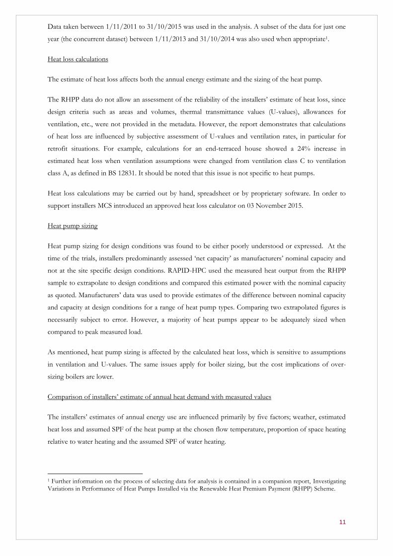
Data taken between 1/11/2011 to 31/10/2015 was used in the analysis. A subset of the data for just one
year (the concurrent dataset) between 1/11/2013 and 31/10/2014 was also used when appropriate1.
Heat loss calculations
The estimate of heat loss affects both the annual energy estimate and the sizing of the heat pump.
The RHPP data do not allow an assessment of the reliability of the installers’ estimate of heat loss, since
design criteria such as areas and volumes, thermal transmittance values (U-values), allowances for
ventilation, etc., were not provided in the metadata. However, the report demonstrates that calculations
of heat loss are influenced by subjective assessment of U-values and ventilation rates, in particular for
retrofit situations. For example, calculations for an end-terraced house showed a 24% increase in
estimated heat loss when ventilation assumptions were changed from ventilation class C to ventilation
class A, as defined in BS 12831. It should be noted that this issue is not specific to heat pumps.
Heat loss calculations may be carried out by hand, spreadsheet or by proprietary software. In order to
support installers MCS introduced an approved heat loss calculator on 03 November 2015.
Heat pump sizing
Heat pump sizing for design conditions was found to be either poorly understood or expressed. At the
time of the trials, installers predominantly assessed ‘net capacity’ as manufacturers’ nominal capacity and
not at the site specific design conditions. RAPID-HPC used the measured heat output from the RHPP
sample to extrapolate to design conditions and compared this estimated power with the nominal capacity
as quoted. Manufacturers’ data was used to provide estimates of the difference between nominal capacity
and capacity at design conditions for a range of heat pump types. Comparing two extrapolated figures is
necessarily subject to error. However, a majority of heat pumps appear to be adequately sized when
compared to peak measured load.
As mentioned, heat pump sizing is affected by the calculated heat loss, which is sensitive to assumptions
in ventilation and U-values. The same issues apply for boiler sizing, but the cost implications of over-
sizing boilers are lower.
Comparison of installers’ estimate of annual heat demand with measured values
The installers’ estimates of annual energy use are influenced primarily by five factors; weather, estimated
heat loss and assumed SPF of the heat pump at the chosen flow temperature, proportion of space heating
relative to water heating and the assumed SPF of water heating.
1 Further information on the process of selecting data for analysis is contained in a companion report, Investigating Variations in Performance of Heat Pumps Installed via the Renewable Heat Premium Payment (RHPP) Scheme.
12
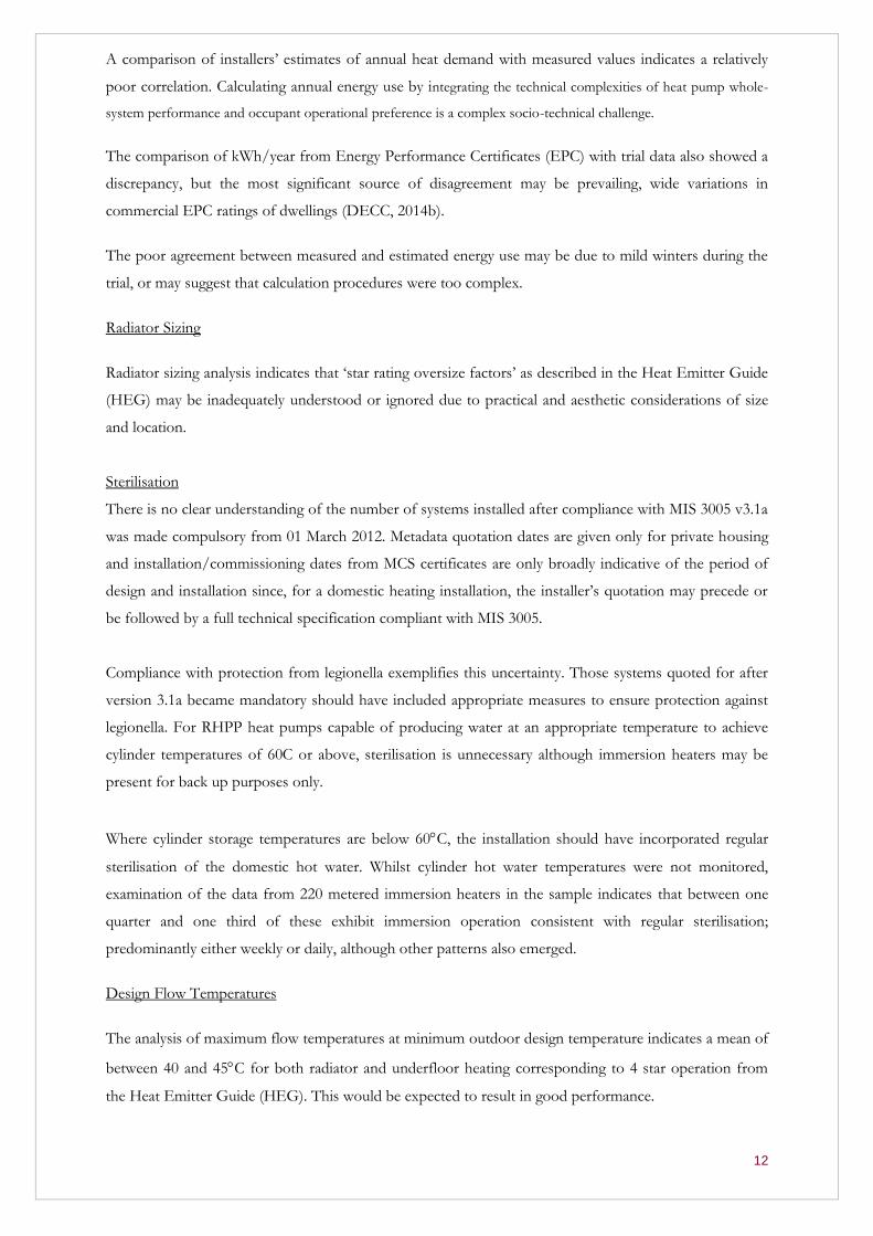
A comparison of installers’ estimates of annual heat demand with measured values indicates a relatively
poor correlation. Calculating annual energy use by integrating the technical complexities of heat pump whole-
system performance and occupant operational preference is a complex socio-technical challenge.
The comparison of kWh/year from Energy Performance Certificates (EPC) with trial data also showed a
discrepancy, but the most significant source of disagreement may be prevailing, wide variations in
commercial EPC ratings of dwellings (DECC, 2014b).
The poor agreement between measured and estimated energy use may be due to mild winters during the
trial, or may suggest that calculation procedures were too complex.
Radiator Sizing
Radiator sizing analysis indicates that ‘star rating oversize factors’ as described in the Heat Emitter Guide
(HEG) may be inadequately understood or ignored due to practical and aesthetic considerations of size
and location.
Sterilisation
There is no clear understanding of the number of systems installed after compliance with MIS 3005 v3.1a
was made compulsory from 01 March 2012. Metadata quotation dates are given only for private housing
and installation/commissioning dates from MCS certificates are only broadly indicative of the period of
design and installation since, for a domestic heating installation, the installer’s quotation may precede or
be followed by a full technical specification compliant with MIS 3005.
Compliance with protection from legionella exemplifies this uncertainty. Those systems quoted for after
version 3.1a became mandatory should have included appropriate measures to ensure protection against
legionella. For RHPP heat pumps capable of producing water at an appropriate temperature to achieve
cylinder temperatures of 60C or above, sterilisation is unnecessary although immersion heaters may be
present for back up purposes only.
Where cylinder storage temperatures are below 60C, the installation should have incorporated regular
sterilisation of the domestic hot water. Whilst cylinder hot water temperatures were not monitored,
examination of the data from 220 metered immersion heaters in the sample indicates that between one
quarter and one third of these exhibit immersion operation consistent with regular sterilisation;
predominantly either weekly or daily, although other patterns also emerged.
Design Flow Temperatures
The analysis of maximum flow temperatures at minimum outdoor design temperature indicates a mean of
between 40 and 45C for both radiator and underfloor heating corresponding to 4 star operation from
the Heat Emitter Guide (HEG). This would be expected to result in good performance.
13
However, a wide range of temperatures is observed; 17% of systems examined had design flow
temperatures of 50-60ºC, indicating 2 or 1 star operation in the HEG, and 34% had design flow
temperatures of <40ºC, indicating 5 or 6 star operation2. Note that regression calculations down to zero
degrees centigrade have been necessary due to the low number of days at design outdoor temperature.
Weather Compensation
The same analysis indicates weather compensation was used for 64% of installations. Weather
compensation is recommended by MCS MIS 3005 version 4.0; however, under some circumstances, for
example, intermittent heating, weather compensation may not be the most effective strategy.
Comparison between measured space heating SPF and Heat Emitter Guide “Likely space heating SPF”
Using the design flow temperatures calculated for each site, the Heat Emitter Guide (HEG) ‘likely space
heating SPF’ has been compared to the actual, measured space heating SPF. Correlations are poor, with
the observed SPF’s being significantly lower than the HEG values. This is more pronounced for GSHP
than ASHP.
In conclusion, MCS heat pump installation standards were updated significantly and on several occasions
during the RHPP period. Any changes inevitably take time to embed. The analysis presented here refers
to the monitored RHPP sample; it should not be assumed to apply to heat pumps installed after the
RHPP.
2 The flow temperature for UFH is a function of the floor and envelope resistances. Tf = {(Tin –Tout) * envelope area/ [floor area * (Rfloor / Renv)]} + Tin Where Tf = flow, Tin and Tout = inside and outside temperature, Rfloor & Renv = thermal resistances of floor and envelope construction. Where, e.g. UFH is embedded in timber floors with carpets, higher flow temperature may be necessary to ensure adequate heat emission.
14
Report on compliance with MCS installation standards 1
Introduction
The Microgeneration Certification Scheme (MCS) is an industry-led, nationally recognised,
BS EN ISO/IEC 17065:2012-compliant quality assurance scheme for microgeneration, launched in 2008.
It publishes product and installation standards, which are periodically updated to reflect evolving
technical understanding. The installation standards specifically relating to heat pumps are MCS MIS 3005,
MCS 021 plus a number of guidance documents relating to estimating heat loss, heat emitter design and
designing ground loops and hydraulics.
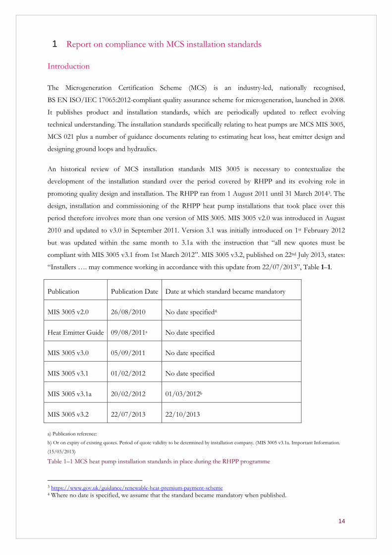
An historical review of MCS installation standards MIS 3005 is necessary to contextualize the
development of the installation standard over the period covered by RHPP and its evolving role in
promoting quality design and installation. The RHPP ran from 1 August 2011 until 31 March 20143. The
design, installation and commissioning of the RHPP heat pump installations that took place over this
period therefore involves more than one version of MIS 3005. MIS 3005 v2.0 was introduced in August
2010 and updated to v3.0 in September 2011. Version 3.1 was initially introduced on 1st February 2012
but was updated within the same month to 3.1a with the instruction that “all new quotes must be
compliant with MIS 3005 v3.1 from 1st March 2012”. MIS 3005 v3.2, published on 22nd July 2013, states:
“Installers …. may commence working in accordance with this update from 22/07/2013”, Table 1–1.
Publication Publication Date Date at which standard became mandatory
MIS 3005 v2.0 26/08/2010 No date specified4
Heat Emitter Guide 09/08/2011a No date specified
MIS 3005 v3.0 05/09/2011 No date specified
MIS 3005 v3.1 01/02/2012 No date specified
MIS 3005 v3.1a 20/02/2012 01/03/2012b
MIS 3005 v3.2 22/07/2013 22/10/2013
a) Publication reference:
b) Or on expiry of existing quotes. Period of quote validity to be determined by installation company. (MIS 3005 v3.1a. Important Information.
(15/03/2013)
Table 1–1 MCS heat pump installation standards in place during the RHPP programme
3 https://www.gov.uk/guidance/renewable-heat-premium-payment-scheme 4 Where no date is specified, we assume that the standard became mandatory when published.
15
The Provisional Report (Wickins, 2014) states of installations referred to in the present report: “the final
sets of meters started reporting valid data in October 2013”, thus establishing v3.2 as the latest probable
version for designing RHPP installations that were included in the RHPP trial. The design and installation
of systems covered by the present report would have involved versions v2.0; v3.0; v3.1a; and possibly
v3.2 of the MIS.
For each installation, there will be some ambiguity over the actual dates when installers changed to the
latest MIS version, since they were allowed to work with the previous version where they had already
provided the quotation/tender. It is expected that the version introduction date varied across
installations, depending mainly on the dates of and time elapsed between the quotation and installation
start date.
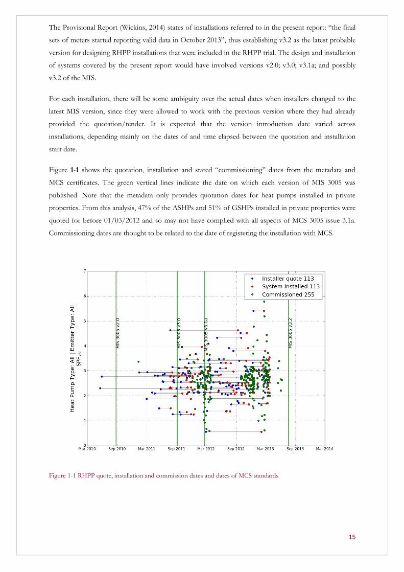
Figure 1-1 shows the quotation, installation and stated “commissioning” dates from the metadata and
MCS certificates. The green vertical lines indicate the date on which each version of MIS 3005 was
published. Note that the metadata only provides quotation dates for heat pumps installed in private
properties. From this analysis, 47% of the ASHPs and 51% of GSHPs installed in private properties were
quoted for before 01/03/2012 and so may not have complied with all aspects of MCS 3005 issue 3.1a.
Commissioning dates are thought to be related to the date of registering the installation with MCS.
Figure 1-1 RHPP quote, installation and commission dates and dates of MCS standards
16
Substantive MIS 3005 changes
This report identifies the development of the MIS 3005 design criteria including the change from earlier
versions that allowed monoenergetic bi-valent systems (to provide non-heat-pump backup during cold
weather) to later versions that require the heat pump to supply 100% of the design-day space heating load
without recourse to the backup heater; the removal of reference to SAP 2005 default SPFs and adjusted
efficiencies; the introduction of BS EN 12831:2003 Heating systems in buildings. Method for calculation
of the design heat load for room by room heat loss calculations; and the publication of the Heat Emitter
Guide (HEG).
MIS v3.0 (09/2011) introduced for the first time a standard method for calculating heat loss and radiatior
sizes and for estimating the system performance5, that is, BS 12831 along with the HEG. In 2011, DECC
supported a series of installer training sessions, the DECC Heat Pump Training road shows. These
included online webinars and spreadsheets produced and presented by David Matthews, then Chief
Executive of the Ground Source Heat Pump Association. Their purpose was to initiate the introduction
of MIS 3005 v3.0 including heat loss calculations based on the CIBSE Domestic heating design guide
(DHDG) and the national annex from BS EN 12831. Whilst BS 12831 provides guidance to the designer,
the calculation of U-values and ventilation rates for heat loss calculations is still dependent on a
qualitative, site-based assessment by the designer. The assessment of e.g. ground floor or window U-
values and air change rates can lead to significant variation in calculated room heat loss and the whole-
house heat pump power needed to satisfy the design day heat load.
The design assessment of SPF is necessary for the calculation of system annual energy use; it is a
requirement of MIS 3005 that annual energy use is calculated and given to customers as part of the
handover. The online webinars show how SPF could be derived from manufacturers’ technical literature
for both space heating and hot water, thus bypassing the use of SAP. However, a review of
manufacturers’ literature from the period shows that relatively few published sufficient COP data to
identify performance at design outside temperature for space heating and design hot water flow
temperatures. In addition, since all published COP values were from BS EN 14511 testing, the
assessment of likely SPF would be based on COP measurements at outside design temperature and
system flow temperature, in effect, a laboratory test condition of fixed source and sink temperatures and
heat sink load (albeit with possible defrost cycle for ASHPs) and thus not reflecting the annual variations
in these factors experienced in real installations. The installer also needs to assess a value for domestic hot
water (DHW) SPF by interpreting COP space heating test results at the most appropriate DHW flow
temperature, such as 55C.
5 MCS 3005 issue 2.0 stated that the installer should provide an estimate of heat loss but gave no details as to what temperature this should be for and contained no information on radiator sizing.
17
The calculation of SPF was rationalised with MIS 3005 v3.1/v3.1a, from which all references to SAP
efficiencies were removed and which required space heating SPF to be assessed using the Heat Emitter
Guide (HEG) based on flow temperatures6. The HEG is a look-up table which allows installers to select a
space heating SPF based on the design heating system flow temperature, calculated through radiator
oversize factors7. The look-up table values for the HEG “likely space heating SPF” are calculated based
on weather conditions for a single location (Leeds, UK) and assuming that “the SPF values for ASHP are
0.7 less than for GSHP, which is consistent with SAP”, plus an allowance of “100W for the electrical
consumption of heating circulation pumps”. The HEG definition of SPF is thus a combination of SPFH2
with circulating pump, or SPFH4 where there is no additional boost. The HEG SPF is for space heating,
“heating circuit flow temperature” with the assumption that flow temperature is weather compensated.
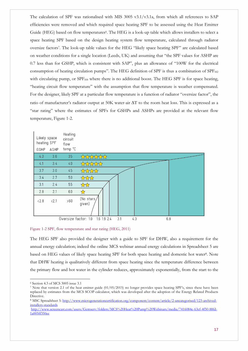
For the designer, likely SPF at a particular flow temperature is a function of radiator “oversize factor”, the
ratio of manufacturer’s radiator output at 50K water-air T to the room heat loss. This is expressed as a
“star rating” where the estimates of SPFs for GSHPs and ASHPs are provided at the relevant flow
temperature, Figure 1-2.
Figure 1-2 SPF, flow temperature and star rating (HEG, 2011)
The HEG SPF also provided the designer with a guide to SPF for DHW, also a requirement for the
annual energy calculation; indeed the online MCS webinar annual energy calculations in Spreadsheet 5 are
based on HEG values of likely space heating SPF for both space heating and domestic hot water8. Note
that DHW heating is qualitatively different from space heating since the temperature difference between
the primary flow and hot water in the cylinder reduces, approximately exponentially, from the start to the
6 Section 4.3 of MCS 3005 issue 3.1 7 Note that version 2.1 of the heat emitter guide (01/05/2015) no longer provides space heating SPF’s, since these have been replaced by estimates from the MCS SCOP calculator, which was developed after the adoption of the Energy Related Products Directive. 8 MSC Spreadsheet 5: http://www.microgenerationcertification.org/component/content/article/2-uncategorised/123-archived-
installers-standards http://www.screencast.com/users/Gemserv/folders/MCS%20Heat%20Pump%20Webinars/media/7416084e-63cf-4f50-88fd-1a005ff350ec

18
end of each heat-up cycle. The instantaneous performance of the heat pump will be determined by the
temperature of the water around the coil, stratification and the location of the indirect heat exchanger coil
within the cylinder. Actual SPF for each DHW cycle will be an integral from the start of the cycle, with
the heat exchanger coil likely surrounded by water at a temperature between room and cold water feed
temperature, to the end of the cycle, when the heat exchanger coil will be surrounded by water close to
the maximum primary water temperature or cylinder thermostat set-point9.
Instantaneous COP for DHW production is covered by BS EN 16147:2011 although, in practice, few
manufacturers of GSHPs and ASHPs provide DHW data. Given that COP for DHW is not available to
the designer, the HEG provides a solution for addressing DHW SPF.
Installer qualifications and handover
MIS 3005 has been the engine for driving enhanced installer training and quality management with the
expectation that such an approach would raise the overall performance of heat pump installations. From
as early as MIS 3005 v1.2 (2008), MCS has demanded a range of specific competences of designers and
installers. Alongside a list of formal qualifications, MCS have been careful not to disadvantage those
working on heat pumps without formal qualifications but who can show accredited prior learning for
registration under the ‘Experienced Worker Route’, through:
Manufacturer’s product training – this is product specific and requires independent verification
Experience gained through a mentoring process – this requires independent verification
Demonstrable track record of successful installation – this requires independent verification
The original competence requirements have since been updated to establish ‘nominated technical’ and
‘designer’ contractual roles along with online qualifications and experience mapping. For MCS company
registration, evidence of these competencies is evaluated by MCS Certification Bodies.
Number of heat pumps, manufacturers and models
Of the total 699 sites in the RHPP sample supplied to RAPID-HPC (referred to as “Sample A”), 99 sites
were excluded at the outset of the project due to technical issues with the metering equipment and a
further 104 sites were omitted due to missing data streams and other issues affecting the calculation of
SPFs. The RHPP sample available for consideration in this analysis therefore comprised 496 sites. A
further series of checks and filters were then applied to generate two sub-samples:
Sample B2 (Broad data) with 417 sites (318 ASHP and 99 GSHPs) with sufficiently complete and
stable (based on circulation rates) monitoring data of the HP system over a year to enable
9 …unless the cylinder thermostat is set to a temperature below the maximum supply temperature from the heat pump. This would represent a failure of commissioning, but it is not impossible.

19
calculation of SPFs. The specific annual period selected for SPF analysis differs from site to site.
Sample C (Concurrent data) with 299 sites (223 ASHP and 76 GSHPs) is a subset of sites in
Sample B, but where data from the same annual monitoring period of 1/11/2013 to 31/10/2014
was selected. Sample C was used for adjustment of data to calculate the SPFs under UKSET
conditions.
This report on compliance with MCS installation standards will use Sample B2 where actual recorded data
provides the clearest explanation of installation performance, and use Sample C where weather corrected
data provides the best solution to the questions posed. RHPP metadata will also be used where
appropriate.
The RHPP MCS certificates show that sample A contains 23 separate manufacturers and up to 115
different heat pump models.
System boundaries and monitored data
Appendix A presents information on system boundaries and monitored data for the RHPP sample.
20
Heat pump sizing; have installers complied with MCS standards? 2
Introduction
Analysis of heat pump sizing for the RHPP must be referenced against the design requirements of
MIS 3005 from version 2.0 to version 3.0 and 3.1a. Before MIS 3005 v 3.0 there was no specific guidance
for designers regarding heat loss calculations and emitter sizing. Any method that the designer thought
appropriate would have satisfied the requirements of MIS 3005 v2.0, whether rule of thumb, a manual
calculator or manufacturers’ software. Version 3.0 introduced the specific requirement that sizing should
comply with the CIBSE Domestic Heating Design Guide (DHDG) and the BS EN 12831 National
Annex.
DHDG and the National annex of BS 12831 are based on fabric and ventilation heat losses as expressed
by (𝜮𝑼𝑨 +𝑵𝑽
𝟑) 𝜟𝑻. Thus a heating system design requires the assessment of U-values (U) for fabric
elements and their areas (A), the assessment of appropriate ventilation rates (N - air changes per hour) for
each room and its volume (V) and the difference between the room temperature and the design outdoor
air temperature for the geographic region (ΔT)10. The designer therefore has to assess three factors in
order to meet MCS criteria: U-values for structural elements, ventilation rates for room-type (living,
kitchen, bedroom, etc) and room temperatures along with the appropriate design outside air temperature
from three sources – the DHDG, BS 12831 and MIS 3005. The designer has to measure the building for
areas and volumes and to complete room-by-room heat loss calculations. Allowances for thermal bridging
(BRE, 2006), and technical underperformance of thermal elements are not specifically addressed in either
the National annex of BS 12831, DHDG or MIS 3005 v3.011.
Following the introduction of MIS 3005 v 3.0, DECC subsidised a series of roadshows and webinars for
installers, exploring heat loss calculations and heat pump sizing. When assessing whether RHPP
installations comply with MCS standards, RAPID-HPC consider it appropriate to reference system design
calculations to this online resource, which can be found on the MCS website12.
Heat loss calculations
Assessing fabric element U-values from the DHDG is not always straightforward. Wall construction in
the UK is generally either solid brick, solid stone or cavity wall. Cavity walls may be brick and brick, or
10 The problem with ventilation heat loss is that, over periods of the order of 24 hours or less, it actually appears mainly in those
rooms in the infiltration zone of the dwelling. Those rooms in the exfiltration zone experience low or no ventilation heat loss. But the respective in/exfiltration zones move around depending on weather conditions. In a 2 storey dwelling, infiltration is mostly downstairs, but on windy days it may be the whole of the windward façade. Thus, the heat output required in each room varies with the weather. This aspect of design is not taken into account in the guides cited. Such calculation techniques have to be seen primarily as pragmatic rather than theoretically consistent representations of heat loss. 11 Party wall heat loss is included, based on the assumption that the other side of the wall is at 10C on average. 12 http://www.microgenerationcertification.org/component/content/article/2-uncategorised/123-archived-installers-standards
21
brick and block where block conductivity varies significantly depending on the block materials. The
eligibility criteria for the RHPP included cavity wall insulation (where appropriate) and at least 250mm of
loft insulation where possible. Commonly used cavity-fill materials include mineral wool, polystyrene
beads and foam, which all have varying thermal properties. The designer will generally not have the
technical specification for the insulation and, allied to the variable quality of installation, must make an
assessment of the likely U-value. The DHDG provides a range of U-values for brick/brick and
brick/block walls with 13 mm plaster and 50 mm mineral fibre-filled cavity from 0.56 to 0.39 W/m2K
resulting in a potential difference of 35%13. Even if the most appropriate value is selected from the
DHDG, the actual performance of the wall is likely to be substantially different. Wingfield et al. (2010)
present measurements of the in situ performance of insulated cavity walls and conclude that the ratio of
actual to design U-values is typically between 1.5 and 2. Hulme and Doran (2014) concluded that the ratio
of actual to RDSAP estimated U-values was between 0.86 and 0.99 for uninsulated cavities (based on 50
homes) and that the ratio for insulated cavity walls was 1.29-1.34 (based on 109 homes). U-values for
solid walls are known to be overestimated in many cases (Li et al. 2014).
Conversely, the DHDG provides a double glazing default of 2.8 W/m2K whereas most double glazed
windows installed since 2002 will outperform this value. For example, 10 year old 12 mm gap double
glazing that complied with Approved Document L1 2000 (DCLG, 2000:23) may have a U value ranging
from 2.8 to 1.8 W/m2K (Table A1). It is therefore possible that estimates of window heat losses may vary
between designers by 40%. Additional losses, such as at window reveals and lintels, may be significant,
and are unlikely to be taken into account.
Ventilation rates offer yet another example of the potential for variation in heat loss assessment. The
DHDG provides design ventilation rates ranging from 3.0 air changes per hour (ac/h) for a bathroom,
2.0 ac/h for a kitchen, 1.5 ac/h for a living room and 1.0 ac/h for a bedroom. These air change rates are
all significantly higher than the whole house ventilation requirement of 0.5 ac/h. MIS 3005 v3.1a suggests
the use of lower ventilation rates where appropriate: “However, this option should only be taken with
caution as field trials indicate these ventilation rates tend to provide good in-use estimates of power and
energy consumption”14. BS 12831 introduces three ventilation categories (A, B and C) based on year of
build – pre-2000, 2000 to 2006 and post 2006 where Category B and C provide 1.0 and 0.5 ac/h for living
rooms. The RHPP required homes to have cavity insulation where practical and statistics from the BRE
Housing tool suggest that they are likely to have had reasonable draught stripping with double glazed
windows that reduce air infiltration15, indicating that lower estimates of ventilation rates may have been
chosen by the installer. Further complexity is introduced for rooms with open fires, a condition identified
in many of the RHPP off-gas grid houses. A 40m2 room with chimney with a throat restrictor, typical of a
wood burner, requires 3 ac/h. 13 Percentage difference = ( (V1 - V2 ) / ((V1 + V2)/2) ) * 100 14 Room heat loss is based on the worst-case assumption that the room is on the windward side of the building (see earlier footnote). This cannot be true for all rooms at the same time, so summing individual room heat losses, will lead to an overestimate of whole house heat loss. This does not invalidate the procedure, whose purpose is purely pragmatic. 15 BRE housing tool indicates that, in 2011-12, 88% of RSL and local authority houses had full double glazing. In the owner occupier sector, the figure was 77%. http://housingdata.bre.co.uk/Home/Crosstab
22
The summation of room losses provides the power required for space heating in continuous mode. For
intermittent heating, an additional allowance of 15% (DHDG) or 20% (BS 12831) is added to the room
heat losses to provide an estimate of the heat pump heat output rating required for the dwelling.
BS 12831 also suggests that for intermittent heating, outdoor design temperature is reduced in accordance
with Table NA.1c External Design Temperatures and resulting in a percentage difference in heat loss of
an additional 1.5 to 2%. The DHDG suggests a further 10% allowance for distribution losses and hot
water allowance from 2.0 to 3.0 kW. We may comment that uninsulated pipes within the insulated
envelope would provide useful space heating during the space heating season whilst primary pipework to
the hot water cylinder (which operates in both winter and summer) has been required to be insulated
under Part L of the Building Regulations for new dwellings since 2002. Observations in the RHPP case
studies indicate that whilst pipe insulation around the heat pump and cylinder is generally provided, the
quality of that insulation is variable. For these reasons it is difficult to say whether that DHDG
recommendations for allowances for distribution losses will be met. Heat pump DHW switching is
generally by diverter valve, since DHW is required at the highest heat pump output temperature. The heat
pump will switch between space heating and DHW rather than supply both at the same time. With
diverter supplied DHW, it is most unlikely that installers would add the hot water power load when sizing
for maximum heat pump output. The situation is best described with an example: for a house with an 8
kW design day heat loss, the additional allowances would result in the selection of a circa 13 kW heat
pump. For heat pumps, unlike for gas boilers, the additional cost of the larger unit output would also be
significant, at approximately 40% of the base case price16.
The final heat loss assessment and heat pump sizing therefore reflects the designer’s technical ability to
navigate through the DHDG, BS 12831 and MIS 3005 as well their commercial judgement when
tendering. Apart from the heat pump specifics of MIS 3005, many of these design decisions apply to
boilers.
Radiator sizing
For the installation designer, maximising heat pump Carnot efficiency is a primarily a function of sink
temperature, that is the temperature of the water flowing to the emitters, whether underfloor heating,
radiators or hot water cylinder17. Thus to maximise the SPF of an installation, a designer should select the
lowest flow temperature consistent with meeting the heat demand of the dwelling. This selection
procedure will comprise several factors including typical default flow temperatures. Providing the
designer understands this relationship, we would expect the selection of radiators to be a compromise
between radiator size (high SPF requires larger radiators) and annual efficiency. Lower temperatures
require larger radiators or, where wall space is limited, progressively higher outputs are achieved for the
16 http://www.airconwarehouse.com/acatalog/Mitsubishi_Ecodan_Air_Source_Heat_Pumps.html 17 Carnot efficiency = Tsink / (Tsink – Tsource) . Actual SPFs are typically around half the Carnot efficiency.
23
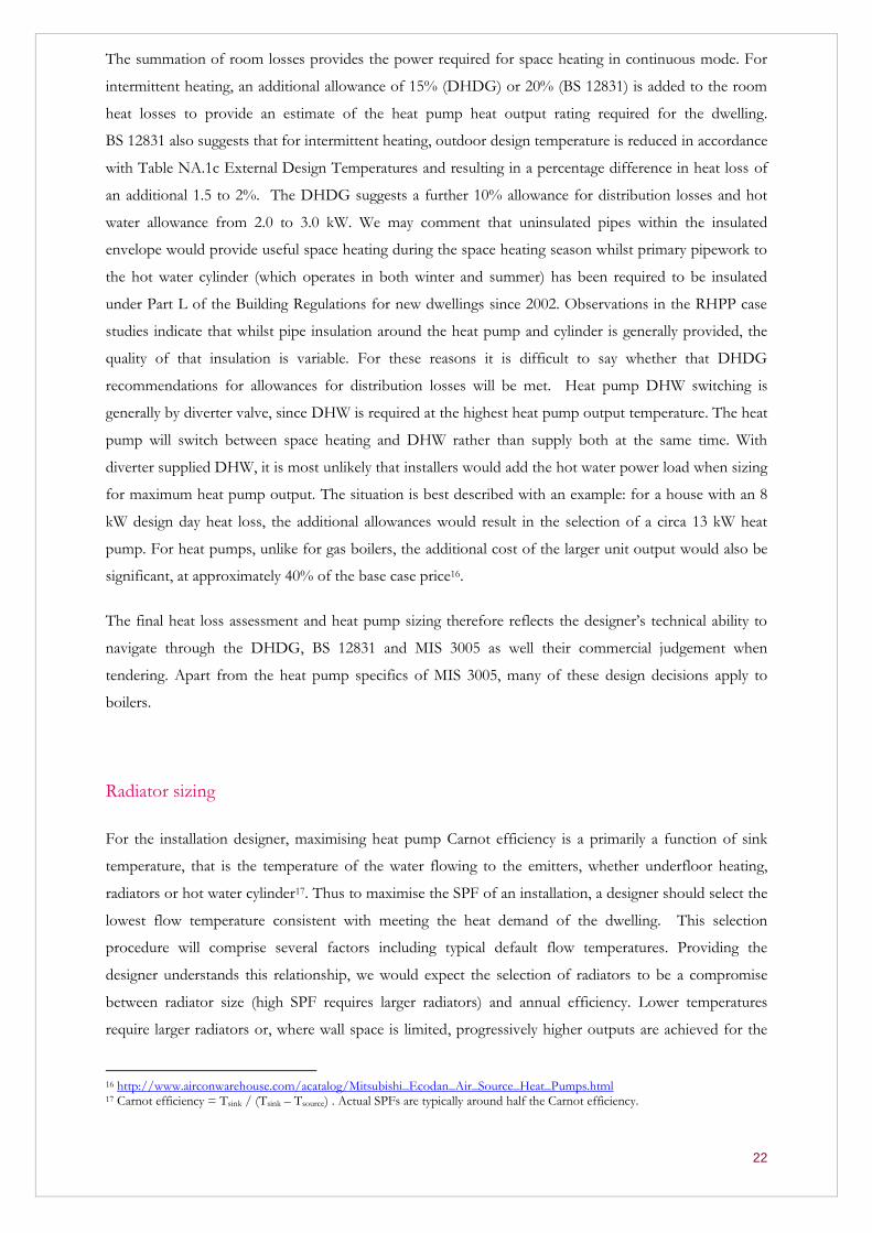
same height and length through the addition of double or triple panels and convectors, Figure 2-1.
Figure 2-1 Example radiator catalogue
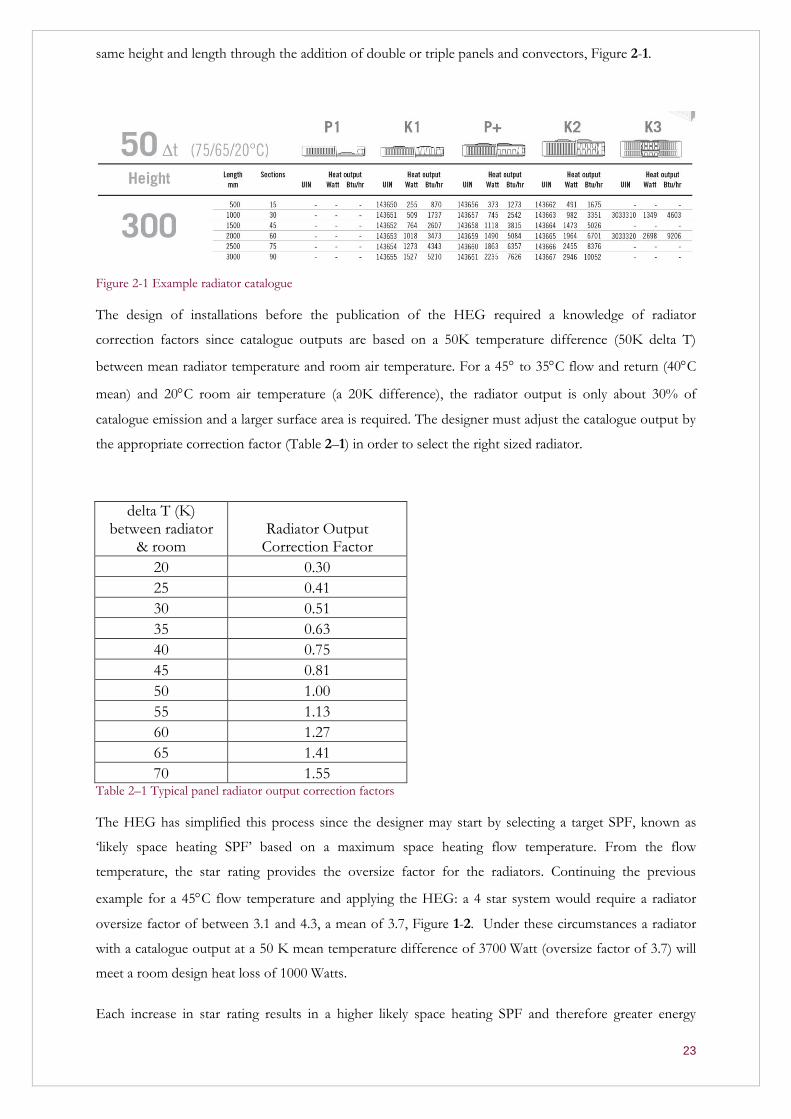
The design of installations before the publication of the HEG required a knowledge of radiator
correction factors since catalogue outputs are based on a 50K temperature difference (50K delta T)
between mean radiator temperature and room air temperature. For a 45 to 35C flow and return (40C
mean) and 20C room air temperature (a 20K difference), the radiator output is only about 30% of
catalogue emission and a larger surface area is required. The designer must adjust the catalogue output by
the appropriate correction factor (Table 2–1) in order to select the right sized radiator.
delta T (K) between radiator
& room Radiator Output
Correction Factor
20 0.30
25 0.41
30 0.51
35 0.63
40 0.75
45 0.81
50 1.00
55 1.13
60 1.27
65 1.41
70 1.55 Table 2–1 Typical panel radiator output correction factors
The HEG has simplified this process since the designer may start by selecting a target SPF, known as
‘likely space heating SPF’ based on a maximum space heating flow temperature. From the flow
temperature, the star rating provides the oversize factor for the radiators. Continuing the previous
example for a 45C flow temperature and applying the HEG: a 4 star system would require a radiator
oversize factor of between 3.1 and 4.3, a mean of 3.7, Figure 1-2. Under these circumstances a radiator
with a catalogue output at a 50 K mean temperature difference of 3700 Watt (oversize factor of 3.7) will
meet a room design heat loss of 1000 Watts.
Each increase in star rating results in a higher likely space heating SPF and therefore greater energy
24
efficiency in annual operation. However, when replacing, for example an oil boiler-fed high temperature
radiator system with low temperature heat pump-fed radiators, achieving a 4 star output is not just a
technical decision of radiator replacement. A typical 600 x 1100 single panel-single convector with an
actual output at 50K of 1078 W cannot be replaced by the same size radiator to achieve a heat pump 4
star design. A 4 star design requires an output at 50K of 3700 Watts and the same size double panel-
double convector or triple panel-triple convector have outputs at 50K of only 1905 W and 2628 W
respectively – they are not large enough. The triple panel would achieve a star rating of only 2.6 (against a
requirement for 3.7) and cost approximately three times as much as the original double panel-single
convector. Achieving a 4 star design would require either more than one radiator or replacing the 600 x
1100 single panel-single convector with a 600 x 1800 triple panel-triple convector with a catalogue output
of 4300 W18. It is worth noting that triple panel-triple convectors of 600 x 1100 and 600 x 1800 weigh
over 50 kg and 80 kg respectively19 with implications for occupational health and safety and increased
labour costs.
It is apparent that, even for the technically competent designer, radiator selection will be based on
multiple factors that include space availability, client demand, room aesthetics and capital and labour cost.
The likely result is that radiator star ratings will vary from room to room as illustrated in Section 2.4.
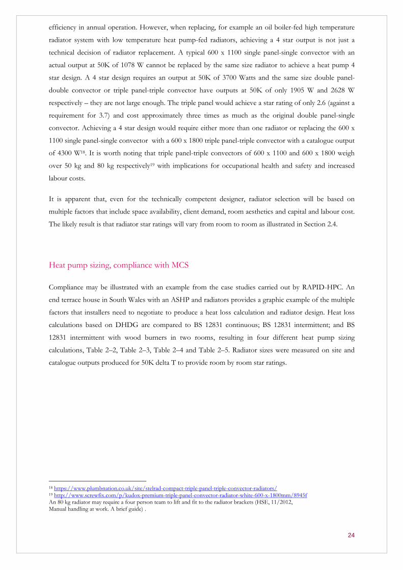
Heat pump sizing, compliance with MCS
Compliance may be illustrated with an example from the case studies carried out by RAPID-HPC. An
end terrace house in South Wales with an ASHP and radiators provides a graphic example of the multiple
factors that installers need to negotiate to produce a heat loss calculation and radiator design. Heat loss
calculations based on DHDG are compared to BS 12831 continuous; BS 12831 intermittent; and BS
12831 intermittent with wood burners in two rooms, resulting in four different heat pump sizing
calculations, Table 2–2, Table 2–3, Table 2–4 and Table 2–5. Radiator sizes were measured on site and
catalogue outputs produced for 50K delta T to provide room by room star ratings.
18 https://www.plumbnation.co.uk/site/stelrad-compact-triple-panel-triple-convector-radiators/ 19 http://www.screwfix.com/p/kudox-premium-triple-panel-convector-radiator-white-600-x-1800mm/8945f An 80 kg radiator may require a four person team to lift and fit to the radiator brackets (HSE, 11/2012, Manual handling at work. A brief guide) .
25
Ventilation (Air-changes
per hour) Room
Heat output at a water-air
T of
50⁰ C20
(Watts) Heat loss (Watts)
Star rating from the
HEG
1.5 Living room total 2868 1087 3
2.0 Kitchen 873 531 2
1.5 Dining room 1598 776 2
1.5 Hall & Landing 1991 767 3
2.0 Bathroom 1055 358 3
1.0 Study 964 401 2
1.0 Small bedroom 852 473 2
1.0 Main bedroom 1106 386 3
HP output
4778 Table 2–2 DHDG estimates of heat loss for continuous heating at -1.6C, ventilation Class A
Ventilation (Air-changes per hour)ac/h Room
Heat output at a water-air
T of 50⁰ C (Watts)
Heat loss (Watts)
Star rating from the
HEG
0.5 Living room total 2868 802 4
1.5 Kitchen 873 477 2
0.5 Dining room 1598 592 3
0.5 Hall & Landing 1991 616 3
1.5 Bathroom 1055 326 3
0.5 Study 964 340 3
0.5 Small bedroom 852 393 2
0.5 Main bedroom 1106 291 4
HP output
3837 Table 2–3 BS 12831 estimates of heat loss for continuous heating at -1.6C, ventilation Class C
Ventilation (Air-changes per hour)ac/h Room
Heat output at a
water-air T of
50⁰ C (Watts)
Heat loss (Watts)
Star rating from the HEG
0.5 Living room total 2868 912 3
1.5 Kitchen 873 633 1
0.5 Dining room 1598 758 2
0.5 Hall & Landing 1991 796 3
1.5 Bathroom 1055 273 4
0.5 Study 964 457 2
0.5 Small bedroom 852 507 2
0.5 Main bedroom 1106 376 3
HP output
4712 Table 2–4 BS 12831 estimates of heat loss for intermittent heating (plus 20%) at -3.2C, ventilation Class C
20 Manufacturers typically quote the output of radiators at a mean radiator-to-room temperature difference of 50K. This is often
referred to as the water-air ΔT. With a temperature difference across the radiator of 10K, and a room temperature of 20C, this
is equivalent to a flow temperature to the radiator of 75C and a return temperature of 65C.
26
Ventilation (Air-changes per hour)ac/h Room
Heat output at a water-air
T of 50⁰ C (Watts)
Heat loss (Watts)
Star rating from the
HEG
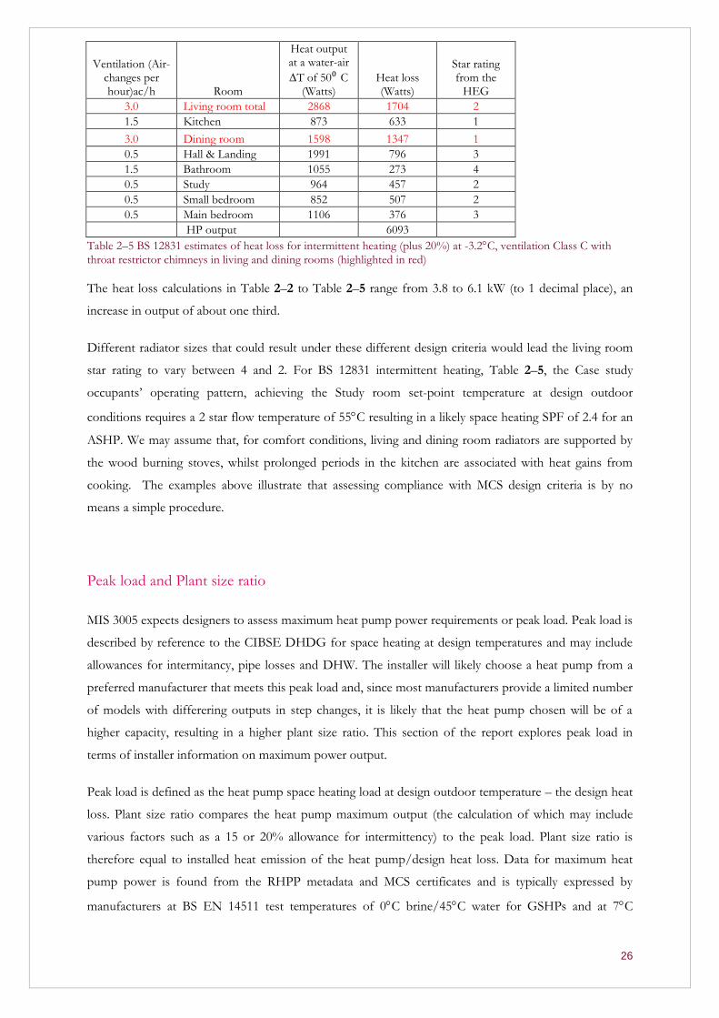
3.0 Living room total 2868 1704 2
1.5 Kitchen 873 633 1
3.0 Dining room 1598 1347 1
0.5 Hall & Landing 1991 796 3
1.5 Bathroom 1055 273 4
0.5 Study 964 457 2
0.5 Small bedroom 852 507 2
0.5 Main bedroom 1106 376 3
HP output
6093 Table 2–5 BS 12831 estimates of heat loss for intermittent heating (plus 20%) at -3.2C, ventilation Class C with
throat restrictor chimneys in living and dining rooms (highlighted in red)
The heat loss calculations in Table 2–2 to Table 2–5 range from 3.8 to 6.1 kW (to 1 decimal place), an
increase in output of about one third.
Different radiator sizes that could result under these different design criteria would lead the living room
star rating to vary between 4 and 2. For BS 12831 intermittent heating, Table 2–5, the Case study
occupants’ operating pattern, achieving the Study room set-point temperature at design outdoor
conditions requires a 2 star flow temperature of 55C resulting in a likely space heating SPF of 2.4 for an
ASHP. We may assume that, for comfort conditions, living and dining room radiators are supported by
the wood burning stoves, whilst prolonged periods in the kitchen are associated with heat gains from
cooking. The examples above illustrate that assessing compliance with MCS design criteria is by no
means a simple procedure.
Peak load and Plant size ratio
MIS 3005 expects designers to assess maximum heat pump power requirements or peak load. Peak load is
described by reference to the CIBSE DHDG for space heating at design temperatures and may include
allowances for intermitancy, pipe losses and DHW. The installer will likely choose a heat pump from a
preferred manufacturer that meets this peak load and, since most manufacturers provide a limited number
of models with differering outputs in step changes, it is likely that the heat pump chosen will be of a
higher capacity, resulting in a higher plant size ratio. This section of the report explores peak load in
terms of installer information on maximum power output.
Peak load is defined as the heat pump space heating load at design outdoor temperature – the design heat
loss. Plant size ratio compares the heat pump maximum output (the calculation of which may include
various factors such as a 15 or 20% allowance for intermittency) to the peak load. Plant size ratio is
therefore equal to installed heat emission of the heat pump/design heat loss. Data for maximum heat
pump power is found from the RHPP metadata and MCS certificates and is typically expressed by
manufacturers at BS EN 14511 test temperatures of 0C brine/45C water for GSHPs and at 7C
27
air/35C water for ASHPs. However, manufacturers’ literature showing output data is not consistent. For
maximum power at design conditions, these power outputs from BS EN 14511 testing need to be
adjusted for the chosen flow temperature. GSHPs, according to MIS 3005, must be designed for a
minimum ground loop flow into the evaporator of 0C; however, for ASHPs, the heat pump maximum
output also needs to be adjusted for COP at outdoor design temperature. It is assumed that for most
installers this would not have proved possible since at the time of installation of the RHPP heat pumps,
many manufacturers did not supply sufficient test data to allow the installer to interpolate power outputs
between maximum (-0.2C, Plymouth) and minimum (-3.9C, Glasgow) outdoor design temperatures
(MIS 3005, Table 2, after CIBSE Guide A Table 2.4). It is therefore assumed that outputs quoted by
installers from the metadata are predominantly those published by manufacturers at standard testing
conditions. In addition, as already noted (Section 2.2) additional allowances for intermittency, pipe losses
and hot water production may have been added to the space heating load. Finally, the designer must
choose a heat pump with an output above that calculated. Thus we would expect the chosen heat pump
output to always exceed the maximum operating load.
Assessing peak heat pump power output at the MIS 3005 outdoor design temperature, “hourly dry-bulb
temperatures equal to or exceeded for 99% of the hours in a year”, is complicated by the lack of heat
pump operating data at these low temperatures. It is also complicated by the time lags inherent in the
opaque fabric of dwellings, which tends to smooth out the effect of variations in external temperature
with periods of less than about 24 hours.
Historically the information from different manufacturers has varied between a single value of kW output
at BS EN 14511-2:2007 ‘Standard rating conditions’ to comprehensive tables and graphs across a range of
source and sink temperatures. In addition to this literature, manufacturers may also produce non-
published information which is made available to heat pump purchasers/registered installers for
extrapolation and interpolation of performance data. Such additional data has not been considered
although it may have some bearing on the conclusions to this section.
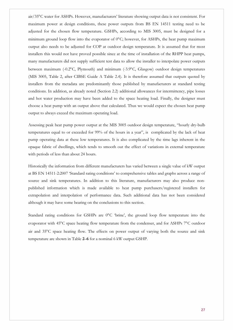
Standard rating conditions for GSHPs are 0C ‘brine’, the ground loop flow temperature into the
evaporator with 45C space heating flow temperature from the condenser, and for ASHPs 7C outdoor
air and 35C space heating flow. The effects on power output of varying both the source and sink
temperature are shown in Table 2–6 for a nominal 6 kW output GSHP.
28
Source
Temperature
Sink Temperature
35C 45C 55C
0C 5.9 kW 5.48 kW 5.17 kW
5C 6.81 kW 6.49 kW 6.08 kW
Table 2–6 GSHP Manufacturer’s capacity data sheet
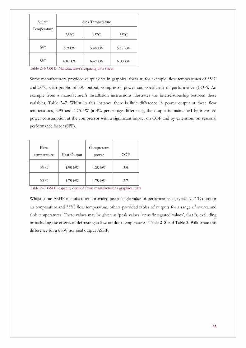
Some manufacturers provided output data in graphical form at, for example, flow temperatures of 35C
and 50C with graphs of kW output, compressor power and coefficient of performance (COP). An
example from a manufacturer’s installation instructions illustrates the interrelationship between these
variables, Table 2–7. Whilst in this instance there is little difference in power output at these flow
temperatures, 4.95 and 4.75 kW (a 4% percentage difference), the output is maintained by increased
power consumption at the compressor with a significant impact on COP and by extension, on seasonal
performance factor (SPF).
Flow
temperature Heat Output
Compressor
power COP
35C 4.95 kW 1.25 kW 3.9
50C 4.75 kW 1.75 kW 2.7
Table 2–7 GSHP capacity derived from manufacturer’s graphical data
Whilst some ASHP manufacturers provided just a single value of performance at, typically, 7C outdoor
air temperature and 35C flow temperature, others provided tables of outputs for a range of source and
sink temperatures. These values may be given as ‘peak values’ or as ‘integrated values’, that is, excluding
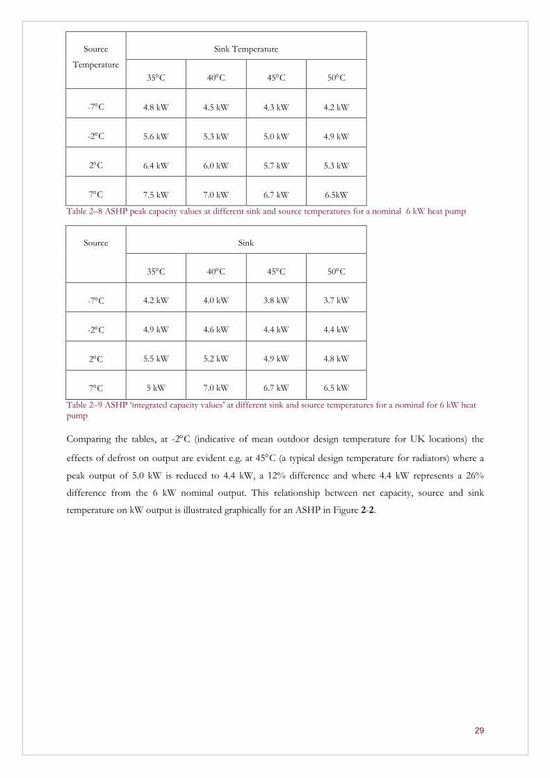
or including the effects of defrosting at low outdoor temperatures. Table 2–8 and Table 2–9 illustrate this
difference for a 6 kW nominal output ASHP.
29
Source
Temperature
Sink Temperature
35C 40C 45C 50C
-7C 4.8 kW 4.5 kW 4.3 kW 4.2 kW
-2C 5.6 kW 5.3 kW 5.0 kW 4.9 kW
2C 6.4 kW 6.0 kW 5.7 kW 5.3 kW
7C 7.5 kW 7.0 kW 6.7 kW 6.5kW
Table 2–8 ASHP peak capacity values at different sink and source temperatures for a nominal 6 kW heat pump
Source Sink
35C 40C 45C 50C
-7C 4.2 kW 4.0 kW 3.8 kW 3.7 kW
-2C 4.9 kW 4.6 kW 4.4 kW 4.4 kW
2C 5.5 kW 5.2 kW 4.9 kW 4.8 kW
7C 5 kW 7.0 kW 6.7 kW 6.5 kW
Table 2–9 ASHP ‘integrated capacity values’ at different sink and source temperatures for a nominal for 6 kW heat pump
Comparing the tables, at -2C (indicative of mean outdoor design temperature for UK locations) the
effects of defrost on output are evident e.g. at 45C (a typical design temperature for radiators) where a
peak output of 5.0 kW is reduced to 4.4 kW, a 12% difference and where 4.4 kW represents a 26%
difference from the 6 kW nominal output. This relationship between net capacity, source and sink
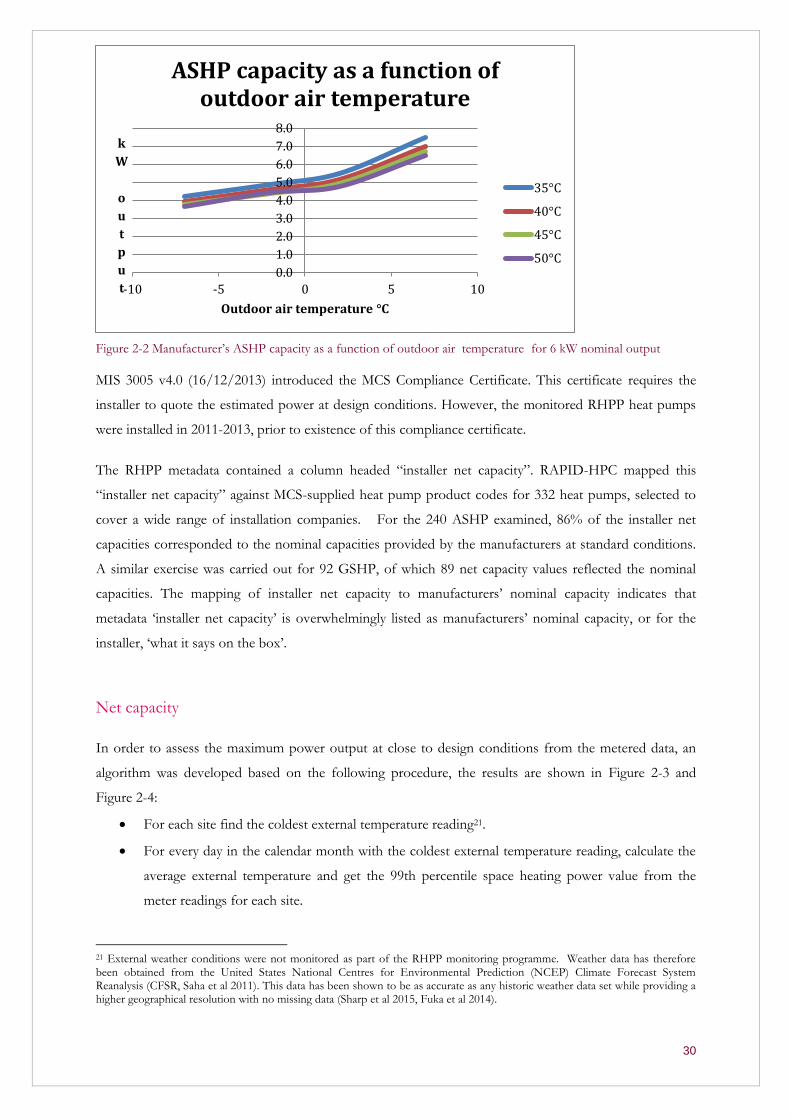
temperature on kW output is illustrated graphically for an ASHP in Figure 2-2.
30
Figure 2-2 Manufacturer’s ASHP capacity as a function of outdoor air temperature for 6 kW nominal output
MIS 3005 v4.0 (16/12/2013) introduced the MCS Compliance Certificate. This certificate requires the
installer to quote the estimated power at design conditions. However, the monitored RHPP heat pumps
were installed in 2011-2013, prior to existence of this compliance certificate.
The RHPP metadata contained a column headed “installer net capacity”. RAPID-HPC mapped this
“installer net capacity” against MCS-supplied heat pump product codes for 332 heat pumps, selected to
cover a wide range of installation companies. For the 240 ASHP examined, 86% of the installer net
capacities corresponded to the nominal capacities provided by the manufacturers at standard conditions.
A similar exercise was carried out for 92 GSHP, of which 89 net capacity values reflected the nominal
capacities. The mapping of installer net capacity to manufacturers’ nominal capacity indicates that
metadata ‘installer net capacity’ is overwhelmingly listed as manufacturers’ nominal capacity, or for the
installer, ‘what it says on the box’.
Net capacity
In order to assess the maximum power output at close to design conditions from the metered data, an
algorithm was developed based on the following procedure, the results are shown in Figure 2-3 and
Figure 2-4:
For each site find the coldest external temperature reading21.
For every day in the calendar month with the coldest external temperature reading, calculate the
average external temperature and get the 99th percentile space heating power value from the
meter readings for each site.
21 External weather conditions were not monitored as part of the RHPP monitoring programme. Weather data has therefore been obtained from the United States National Centres for Environmental Prediction (NCEP) Climate Forecast System Reanalysis (CFSR, Saha et al 2011). This data has been shown to be as accurate as any historic weather data set while providing a higher geographical resolution with no missing data (Sharp et al 2015, Fuka et al 2014).
0.0
1.0
2.0
3.0
4.0
5.0
6.0
7.0
8.0
-10 -5 0 5 10
k
W
o
u
t
p
u
t
Outdoor air temperature °C
ASHP capacity as a function of outdoor air temperature
35°C
40°C
45°C
50°C

31
These values are plotted in the top right hand panel. There are therefore approximately 30 points
per site.
Weather compensation curves are essentially straight line plots providing space heating supply or
return temperature against the difference between room and outdoor temperature (for derivation
of curves see Appendix C). We therefore fit a straight line and extrapolate down to zero degrees
(0C) external temperature to provide the expected peak heating power output at a daily average
temperature of zero degrees to model low outdoor temperature performance. The straight line fit
is sensitive to uncertainties in the space heat readings and the external temperature estimates. If
some of the data has been corrupted it is possible for the gradient to be miscalculated as zero or
even positive, meaning that, un-realistically, heat output increases as external temperature rises.
Those sites where a negative gradient is not returned are given a peak space heating power output
equivalent to the maximum daily value of the coldest month. This extrapolated peak heating
power output at a daily average temperature of 0C is shown on the bottom righthand chart.
We consider that the peak heating power at an average daily temperature of 0ºC will occur when
the hourly external temperature is comparable to, or lower than, the design temperatures for
maximum flow rate in MCS (-0.2ºC for Plymouth, -3.9ºC for Glasgow). Therefore, extrapolation
of peak heating output to a daily average temperature of 0ºC will provide a rough estimate of the
peak heating power at the MCS design temperature.
Installer net capacity is shown in the top left hand side.
A scatter plot is created of peak heating power versus Installer-estimated net capacity, shown on
the bottom left hand side. The line is to guide the eye and shows what a one-to-one mapping
would be. For Figure 2-4 the red dots identify those systems with unmetered resistance boost
producing more than 10% of annual heat output.
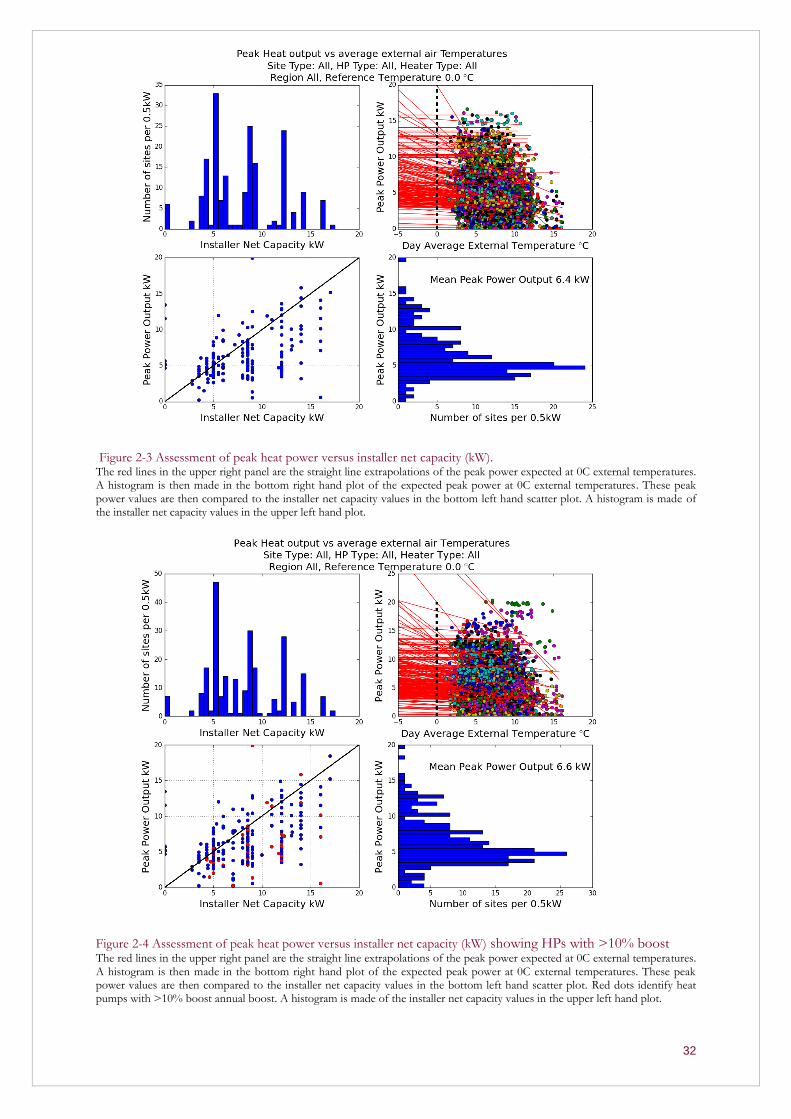
32
Figure 2-3 Assessment of peak heat power versus installer net capacity (kW). The red lines in the upper right panel are the straight line extrapolations of the peak power expected at 0C external temperatures. A histogram is then made in the bottom right hand plot of the expected peak power at 0C external temperatures. These peak power values are then compared to the installer net capacity values in the bottom left hand scatter plot. A histogram is made of the installer net capacity values in the upper left hand plot.
Figure 2-4 Assessment of peak heat power versus installer net capacity (kW) showing HPs with >10% boost The red lines in the upper right panel are the straight line extrapolations of the peak power expected at 0C external temperatures. A histogram is then made in the bottom right hand plot of the expected peak power at 0C external temperatures. These peak power values are then compared to the installer net capacity values in the bottom left hand scatter plot. Red dots identify heat pumps with >10% boost annual boost. A histogram is made of the installer net capacity values in the upper left hand plot.

33
The bottom left hand side scatter plots in Figure 2-3 and Figure 2-4 show the peak capacity at a mean
daily external temperature of 0C as a function of installer net capacity or “installer net power” as written
on the MCS certificate. As noted previously, at the time of the RHPP installation not all manufacturers
provided the required tables or charts to allow installers to estimate the power at design conditions. The
procedure to do so was described in the Matthews webinars22. In practice, it is not possible to assess how
many of the installers actually estimated the power at design conditions; the new MCS compliance
certificate includes an explicit requirement to do this. The requirement for meeting heat output at design
conditions was introduced in MIS 3005 v3.0 (05/09/2011: Section 4.2.1.c). Downloadable MCS
spreadsheet certificates explicitly demanding the heat output at design conditions were introduced in MIS
3005 v4.0 (16/12/2013: Section 6.1).
In general, and particularly for fixed speed compressor ASHPs, the capacity at design conditions of -2C
(the mean outdoor design temperature for MIS 3005 UK locations) is demonstrably lower than
manufacturer nominal output or badged capacity. For five fixed speed compressor ASHP models the
capacity at design conditions drops by between -8% and -32% depending on the model and flow
temperature chosen.
For the two variable speed ASHP models examined, the capacity at design conditions (as calculated from
manufacturers’ data) is reduced by as little as -2% to -4% for one manufacturer but by -20% to -31% for
another.
For GSHPs MIS 3005 design criteria is based on a minimum ground loop temperature 0C and since
manufacturers provide COP data at this temperature no interpolation based on source is required. Output
however will vary depending on flow temperature. BS EN 14581 standard rating conditions provide 0/45
for ‘brine’ source (water with antifreeze) GSHPs. For the 10 GSHP models examined, the listed capacity
at 0/45 was generally different from the manufacturer’s nominal capacity and varied between plus 5% and
minus 23%. Similarly, variations in output are found for 0/35, varying from plus 10% to minus 12% . For
a more complete description of output at design temperature see Appendix B.
The impact on output at design temperature, explored in Figure 2–3 and Figure 2–4 and shown in the
bottom left hand side chart, demonstrates that some heat pumps in the sample are clearly undersized
according to MIS criteria. In order to determine whether the remainder of the heat pumps in the sample
are under or oversized, the corrections from nominal capacity to capacity at design conditions would have
to be applied to the x-value of each point on the chart. As described in Appendix B, these corrections
depend on the make and model of heat pump; for the models examined, we found a range from -2% to -
32% for ASHP and from -23% to +10% for GSHP. This calculation has not been carried out. As a result,
we are not able to make a more precise assessment of how many of the heat pumps in the sample were
22 MCS Heat Pump Webinars, MIS 3005 v3 Spreadsheet – 5: http://www.screencast.com/t/s13i9Nrmp7

34
under or over-sized relative to the MCS criteria. However, there are some points for which the inferred
design capacity is much lower than the nominal “net” capacity, which would indicate over-sizing.
Load Factor
As a short digression from the analysis of MCS proper, the analysis of RHPP data for load factor offers
the opportunity to consider the impact on annual operation at low loads and hence any connection
between annual heat output and SPF. The Heat emitter guide provides likely space heating SPF for a
range of flow temperatures whereas analysis of load factor may indicate that annual heat output may also
affect SPF. As defined by DECC (2010) – ‘the load factor on an unchanged configuration basis for a
calendar year’, is calculated from:
𝑳𝒐𝒂𝒅 𝑭𝒂𝒄𝒕𝒐𝒓 =
"𝑺𝒖𝒎 𝒐𝒇 𝒉𝒆𝒂𝒕 𝒐𝒖𝒕𝒑𝒖𝒕 𝒊𝒏 𝑾𝒉 𝒑𝒆𝒓 𝒚𝒆𝒂𝒓"𝟏𝟎𝟎𝟎 𝑾𝒉 𝒑𝒆𝒓 𝒌𝑾𝒉
"installer Net capacity kW" × 𝟖𝟕𝟔𝟎 𝒉𝒐𝒖𝒓𝒔 𝒑𝒆𝒓 𝒚𝒆𝒂𝒓× 𝟏𝟎0
𝑳𝑭 =𝒌𝑾𝒉 𝒂𝒄𝒕𝒖𝒂𝒍
𝒌𝑾𝒉 𝒑𝒐𝒕𝒆𝒏𝒕𝒊𝒂𝒍× 𝟏𝟎𝟎%
The load factor for heat pumps, therefore, is based on heat energy generated and is defined as the ratio of
produced energy (kWh) to the maximum possible energy output (kWh) over a year. Data for maximum
energy is derived from the nominal heat pump power as found from the RHPP metadata and MCS
certificates.
Load factors are shown for all heat pumps in Figure 2-5; for ASHPs in Figure 2-6; and for GSHPs in
Figure 2-7.
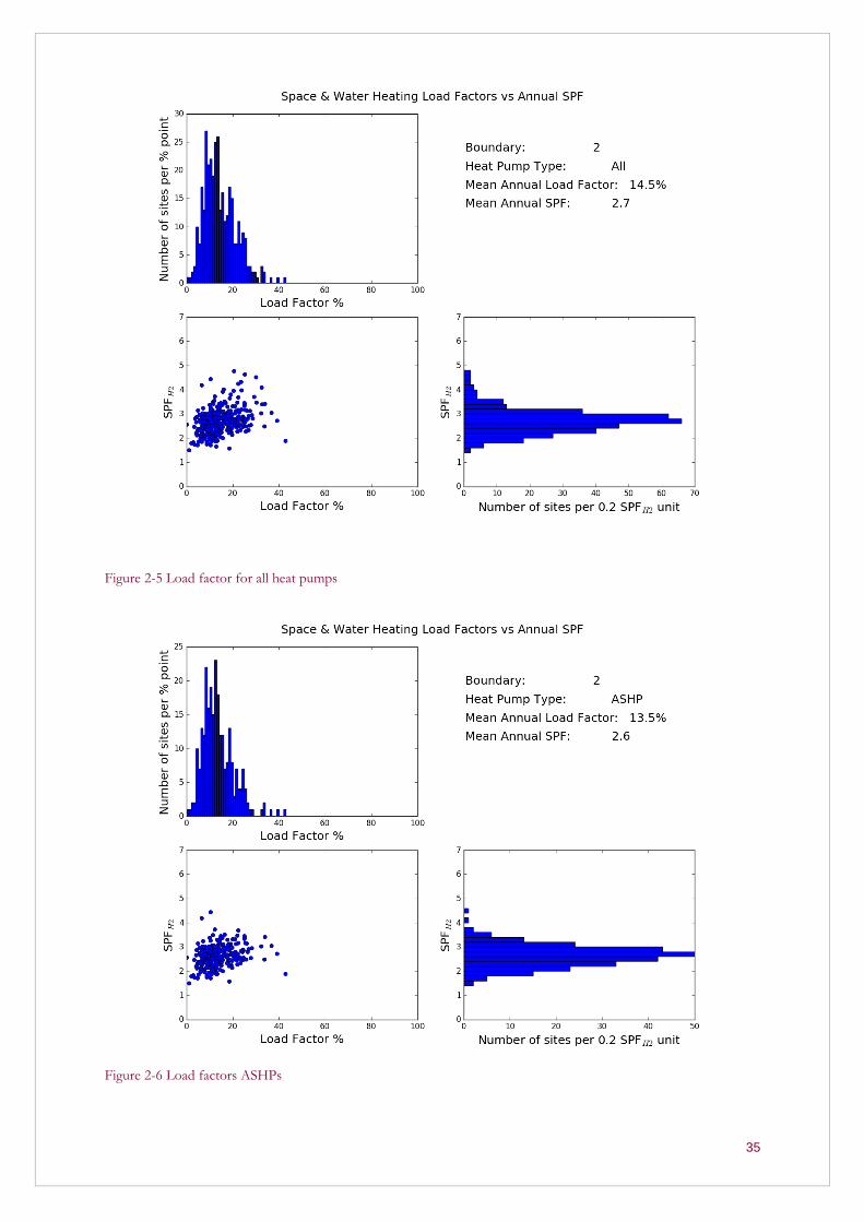
35
Figure 2-5 Load factor for all heat pumps
Figure 2-6 Load factors ASHPs
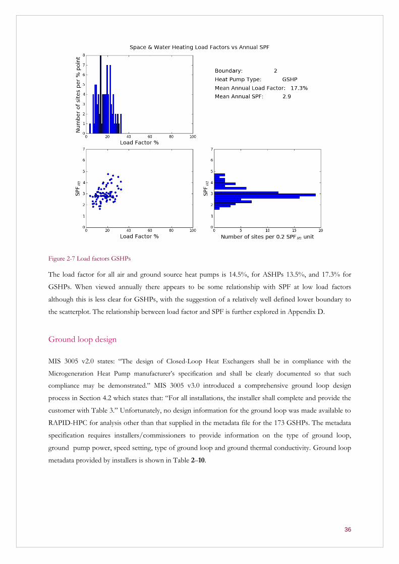
36
Figure 2-7 Load factors GSHPs
The load factor for all air and ground source heat pumps is 14.5%, for ASHPs 13.5%, and 17.3% for
GSHPs. When viewed annually there appears to be some relationship with SPF at low load factors
although this is less clear for GSHPs, with the suggestion of a relatively well defined lower boundary to
the scatterplot. The relationship between load factor and SPF is further explored in Appendix D.
Ground loop design
MIS 3005 v2.0 states: “The design of Closed-Loop Heat Exchangers shall be in compliance with the
Microgeneration Heat Pump manufacturer’s specification and shall be clearly documented so that such
compliance may be demonstrated.” MIS 3005 v3.0 introduced a comprehensive ground loop design
process in Section 4.2 which states that: “For all installations, the installer shall complete and provide the
customer with Table 3.” Unfortunately, no design information for the ground loop was made available to
RAPID-HPC for analysis other than that supplied in the metadata file for the 173 GSHPs. The metadata
specification requires installers/commissioners to provide information on the type of ground loop,
ground pump power, speed setting, type of ground loop and ground thermal conductivity. Ground loop
metadata provided by installers is shown in Table 2–10.
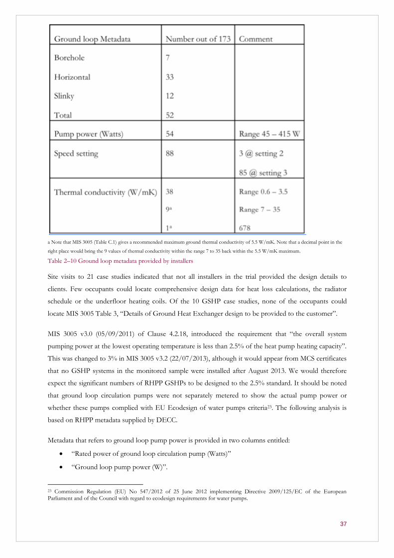
37
a Note that MIS 3005 (Table C.1) gives a recommended maximum ground thermal conductivity of 5.5 W/mK. Note that a decimal point in the
right place would bring the 9 values of thermal conductivity within the range 7 to 35 back within the 5.5 W/mK maximum.
Table 2–10 Ground loop metadata provided by installers
Site visits to 21 case studies indicated that not all installers in the trial provided the design details to
clients. Few occupants could locate comprehensive design data for heat loss calculations, the radiator
schedule or the underfloor heating coils. Of the 10 GSHP case studies, none of the occupants could
locate MIS 3005 Table 3, “Details of Ground Heat Exchanger design to be provided to the customer”.
MIS 3005 v3.0 (05/09/2011) of Clause 4.2.18, introduced the requirement that “the overall system
pumping power at the lowest operating temperature is less than 2.5% of the heat pump heating capacity”.
This was changed to 3% in MIS 3005 v3.2 (22/07/2013), although it would appear from MCS certificates
that no GSHP systems in the monitored sample were installed after August 2013. We would therefore
expect the significant numbers of RHPP GSHPs to be designed to the 2.5% standard. It should be noted
that ground loop circulation pumps were not separately metered to show the actual pump power or
whether these pumps complied with EU Ecodesign of water pumps criteria23. The following analysis is
based on RHPP metadata supplied by DECC.
Metadata that refers to ground loop pump power is provided in two columns entitled:
“Rated power of ground loop circulation pump (Watts)”
“Ground loop pump power (W)”.
23 Commission Regulation (EU) No 547/2012 of 25 June 2012 implementing Directive 2009/125/EC of the European Parliament and of the Council with regard to ecodesign requirements for water pumps.
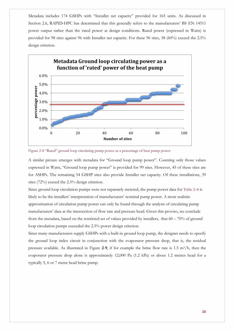
38
Metadata includes 174 GSHPs with “Installer net capacity” provided for 165 units. As discussed in
Section 2.6, RAPID-HPC has determined that this generally refers to the manufacturers’ BS EN 14511
power output rather than the rated power at design conditions. Rated power (expressed in Watts) is
provided for 98 sites against 96 with Installer net capacity. For these 96 sites, 58 (60%) exceed the 2.5%
design criterion.
Figure 2-8 “Rated” ground loop circulating pump power as a percentage of heat pump power
A similar picture emerges with metadata for “Ground loop pump power”. Counting only those values
expressed in Watts, “Ground loop pump power” is provided for 99 sites. However, 45 of these sites are
for ASHPs. The remaining 54 GSHP sites also provide Installer net capacity. Of these installations, 39
sites (72%) exceed the 2.5% design criterion.
Since ground loop circulation pumps were not separately metered, the pump power data for Table 2–8 is
likely to be the installers’ interpretation of manufacturers’ nominal pump power. A more realistic
approximation of circulation pump power can only be found through the analysis of circulating pump
manufacturers’ data at the intersection of flow rate and pressure head. Given this proviso, we conclude
from the metadata, based on the restricted set of values provided by installers, that 60 – 70% of ground
loop circulation pumps exceeded the 2.5% power design criterion.
Since many manufacturers supply GSHPs with a built-in ground loop pump, the designer needs to specify
the ground loop index circuit in conjunction with the evaporator pressure drop, that is, the residual
pressure available. As illustrated in Figure 2-9, if for example the brine flow rate is 1.5 m3/h, then the
evaporator pressure drop alone is approximately 12,000 Pa (1.2 kPa) or about 1.2 metres head for a
typically 5, 6 or 7 metre head brine pump.
0.0%
1.0%
2.0%
3.0%
4.0%
5.0%
6.0%
0 20 40 60 80 100
pe
rce
nta
ge
po
we
r
Number of sites
Metadata Ground loop circulating power as a function of 'rated' power of the heat pump
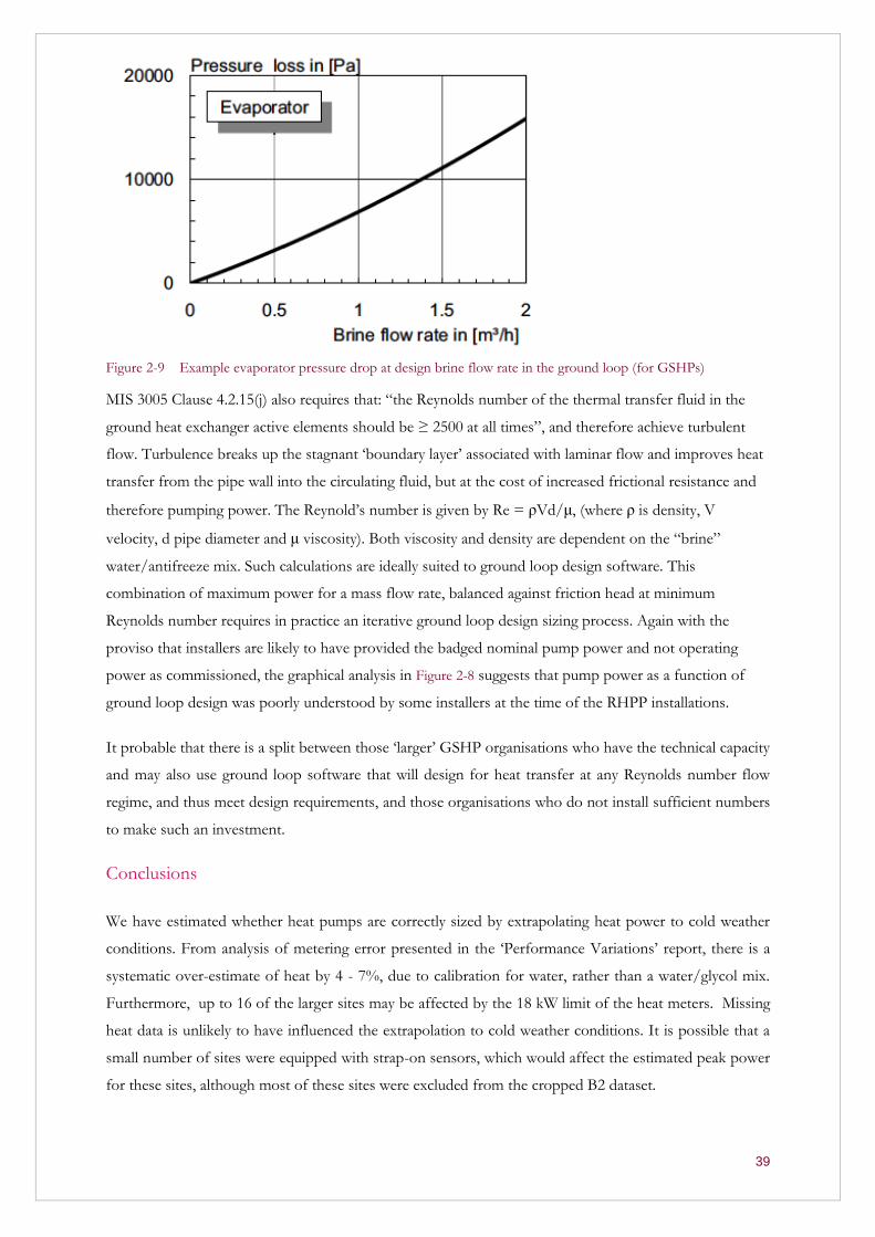
39
Figure 2-9 Example evaporator pressure drop at design brine flow rate in the ground loop (for GSHPs)
MIS 3005 Clause 4.2.15(j) also requires that: “the Reynolds number of the thermal transfer fluid in the
ground heat exchanger active elements should be ≥ 2500 at all times”, and therefore achieve turbulent
flow. Turbulence breaks up the stagnant ‘boundary layer’ associated with laminar flow and improves heat
transfer from the pipe wall into the circulating fluid, but at the cost of increased frictional resistance and
therefore pumping power. The Reynold’s number is given by Re = ρVd/μ, (where ρ is density, V
velocity, d pipe diameter and μ viscosity). Both viscosity and density are dependent on the “brine”
water/antifreeze mix. Such calculations are ideally suited to ground loop design software. This
combination of maximum power for a mass flow rate, balanced against friction head at minimum
Reynolds number requires in practice an iterative ground loop design sizing process. Again with the
proviso that installers are likely to have provided the badged nominal pump power and not operating
power as commissioned, the graphical analysis in Figure 2-8 suggests that pump power as a function of
ground loop design was poorly understood by some installers at the time of the RHPP installations.
It probable that there is a split between those ‘larger’ GSHP organisations who have the technical capacity
and may also use ground loop software that will design for heat transfer at any Reynolds number flow
regime, and thus meet design requirements, and those organisations who do not install sufficient numbers
to make such an investment.
Conclusions
We have estimated whether heat pumps are correctly sized by extrapolating heat power to cold weather
conditions. From analysis of metering error presented in the ‘Performance Variations’ report, there is a
systematic over-estimate of heat by 4 - 7%, due to calibration for water, rather than a water/glycol mix.
Furthermore, up to 16 of the larger sites may be affected by the 18 kW limit of the heat meters. Missing
heat data is unlikely to have influenced the extrapolation to cold weather conditions. It is possible that a
small number of sites were equipped with strap-on sensors, which would affect the estimated peak power
for these sites, although most of these sites were excluded from the cropped B2 dataset.

40
The analysis of heat loss calculations shows that, even when using BS 12831, compliance is not an ‘exact
science’ especially when retrofitting in existing housing with unknown U-values and ventilation rates.
Radiator sizing has been shown to depend as much on the exigencies of property and client as on formal
compliance with a single ‘star rating’ output. The RHPP metadata provides predominantly badged heat
pump capacity as opposed to capacity at design conditions. Any analysis of installer ability to heat pump
size is compromised by the lack of detailed dwelling heat loss characteristics such as floor area or year of
build. Similarly, the lack of ground loop design calculations and limited metadata throws into question any
quantitative conclusions regarding compliance. The step-change in design criteria iniated in MIS 3005
v3.0 demanded of installer companies the necessary calculation methodologies to ensure quality assurance
of all MCS installations against a background of a largely unregulated design approach. For those
companies specialising in heat pump installations, where design procedures were well understood and
may already have been supported by specialist software, such changes were likely welcomed as
recognition that heat performance is sensitive to design, installation and operation. For those companies
installing the occasional heat pump the additional demands for MIS 3005 compliance could certainly have
required investment in new knowledge and working practices. That the changes occurred during the trials
complicates any assessment of their impact on RHPP performance since their effects are likely to require
a period of adjustment. Thus a poor understanding of formal design criteria in 2012 does not imply a
poor understanding in 2016.
41
How do actual space and water heating demand compare to the estimated 3
figures on the MCS certificate and on the EPC?
Introduction
The installer is expected to assess annual energy performance (kWh/year) for contractual purposes. The
calculation for space heating is based on degree day region, building form and fabric, occupant usage
patterns and system efficiency. The calculation for energy required for domestic hot water is based on the
likely daily hot water use, the maximum temperature achievable by heat pump only (and thus the likely
DHW SPF) and any additional energy required for regular pasteurisation by a resistance heater to meet
health and safety demands for legionella protection. The assessment of annual energy for MCS
compliance may have been unfamiliar to many installers since it is not a demand for either gas or oil
heating systems. Hence MIS 3005, as early as v1.2 (25/02/08), has provided an annual energy assessment
method:
The means of estimating the annual energy performance is as follows:
a) Assess the annual heat load for the building (space heating or hot water) using any suitable
performance calculation method. Such calculation method shall be clearly described and justified.
b) Multiply the result from a) by the proportion of the relevant heat load provided by the
Microgeneration Heat Pump system as determined in accordance with Clause 4.2.1.
c) Divide the result from b) by the default efficiency (expressed as a Coefficient of Performance or CoP)
for Heat Pumps contained in SAP 2005 Table 4a (note: CoPs corrected for Heat Pumps with auxiliary
heaters should not be used).
d) Divide the result from c) by the appropriate efficiency adjustment contained in Table 4c of SAP 2005.
e) Calculate the energy supplied by the auxiliary heater by multiplying the result from a) by the proportion
of the relevant heat load not supplied by the Heat Pump.
f) Add the result from d) to the result from e) to give the total energy required for the relevant heat load.
g) The results from f) for space heating and hot water are added together to give an overall energy
requirement for the building for these heat loads.
We note that by dividing the annual space heating and hot water load by the “efficiency” the resulting
annual energy performance is the electrical “energy required”, from which the installer may directly
estimate annual running costs.
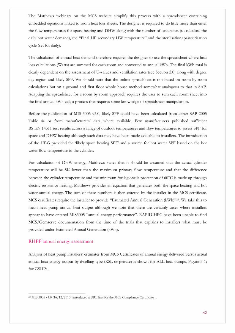
42
The Matthews webinars on the MCS website simplify this process with a spreadsheet containing
embedded equations linked to room heat loss sheets. The designer is required to do little more than enter
the flow temperatures for space heating and DHW along with the number of occupants (to calculate the
daily hot water demand), the “Final HP secondary HW temperature” and the sterilisation/pasteurisation
cycle (set for daily).
The calculation of annual heat demand therefore requires the designer to use the spreadsheet where heat
loss calculations (Watts) are summed for each room and converted to annual kWh. The final kWh total is
clearly dependent on the assessment of U-values and ventilation rates (see Section 2.0) along with degree
day region and likely SPF. We should note that the online spreadsheet is not based on room-by-room
calculations but on a ground and first floor whole house method somewhat analogous to that in SAP.
Adapting the spreadsheet for a room by room approach requires the user to sum each room sheet into
the final annual kWh cell; a process that requires some knowledge of spreadsheet manipulation.
Before the publication of MIS 3005 v3.0, likely SPF could have been calculated from either SAP 2005
Table 4a or from manufacturers’ data where available. Few manufacturers published sufficient
BS EN 14511 test results across a range of outdoor temperatures and flow temperatures to assess SPF for
space and DHW heating although such data may have been made available to installers. The introduction
of the HEG provided the ‘likely space heating SPF’ and a source for hot water SPF based on the hot
water flow temperature to the cylinder.
For calculation of DHW energy, Matthews states that it should be assumed that the actual cylinder
temperature will be 5K lower than the maximum primary flow temperature and that the difference
between the cylinder temperature and the minimum for legionella protection of 60C is made up through
electric resistance heating. Matthews provides an equation that generates both the space heating and hot
water annual energy. The sum of these numbers is then entered by the installer in the MCS certificate.
MCS certificates require the installer to provide “Estimated Annual Generation (kWh)”24. We take this to
mean heat pump annual heat output although we note that there are certainly cases where installers
appear to have entered MIS3005 “annual energy performance”. RAPID-HPC have been unable to find
MCS/Gemserve documentation from the time of the trials that explains to installers what must be
provided under Estimated Annual Generation (kWh).
RHPP annual energy assessment
Analysis of heat pump installers’ estimates from MCS Certificates of annual energy delivered versus actual
annual heat energy output by dwelling type (RSL or private) is shown for ALL heat pumps, Figure 3-1;
for GSHPs,
24 MIS 3005 v4.0 (16/12/2013) introduced a URL link for the MCS Compliance Certificate . .
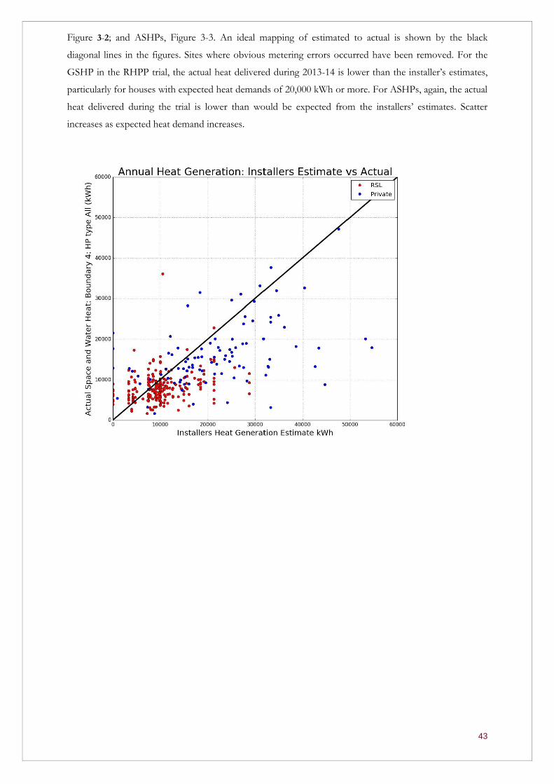
43
Figure 3-2; and ASHPs, Figure 3-3. An ideal mapping of estimated to actual is shown by the black
diagonal lines in the figures. Sites where obvious metering errors occurred have been removed. For the
GSHP in the RHPP trial, the actual heat delivered during 2013-14 is lower than the installer’s estimates,
particularly for houses with expected heat demands of 20,000 kWh or more. For ASHPs, again, the actual
heat delivered during the trial is lower than would be expected from the installers’ estimates. Scatter
increases as expected heat demand increases.
60000
« 50000
'" C. 0-~
c.. I
q- 40000
~ '" "0 C :J o
CO 30000 ;..;
'" '" I
,OJ ~ 20000
"0 C
'" '" U
~ 10000 Vl
'" :J
~
Annual Heat Generation: Installers Estimate vs Actual
o
,-
o
o 00
••••• . . .. :" :: • •• 1 :.. ~ . • •• .. .'.. .
.• , ,: .. :;, -i \.... • 0
V-•••• o 0
•• • • o
o o
o .. o
o
o
o 0 o o
o
o o o
o
• o
o
o
o
10000 20000 30000 40000 50000
Installers Heat Generation Estimate kWh
o
o
60000
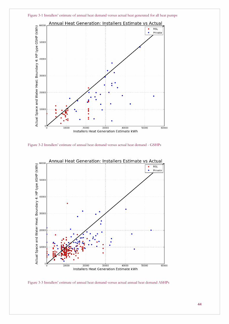
44
Figure 3-1 Installers’ estimate of annual heat demand versus actual heat generated for all heat pumps
Figure 3-2 Installers’ estimate of annual heat demand versus actual heat demand - GSHPs
Figure 3-3 Installers’ estimate of annual heat demand versus actual annual heat demand ASHPs
45
Figure 3-4 Difference between MCS predicted and actual heat energy for ASHPs and GSHPs
EPC annual energy assessment
The RHPP trial required an energy performance certificate (EPC) to be provided as part of the quality
control process. EPCs provide an assessment of annual energy demand based on either SAP for new
build or the reduced version RDSAP for existing properties. BEIS have provided RAPID-HPC with
EPCs for the RHPP sites in order to compare EPC estimated heat demand with actual heat demand and
to compare EPC demand with MCS demand. A series of scatter plots illustrating these relationships are
provided below. Figure 3-5 illustrates EPC predicted space heating for all heat pumps with measured heat
output and shows quite reasonable mapping up to 10,000 kWh/year, but a tendency to over-estimate
demand above this level. It is possible to speculate that that this results from technical inaccuracies such
as from solid wall U-values (Li, et al, 2014) or from social issues associated with heating poorly insulated
or larger houses. It may be that larger houses provide occupants with more options for occupancy and
heating patterns. We also note in passing that some EPC certificates record very low energy demand.
The EPC assessment of domestic hot water heat demand, Figure 3-6 is clustered around 2,500 to
3,000 kWh/year where measured demand ranges from almost none through to 15,000 kWh/year. Actual
hot water use is highly dependent on number of occupants and presence of children in the household.
Adding complexity is the role of showering versus bathing and, as observed in the RHPP case studies, the
use of unmetered electric showers, which may have the effect of reducing the amount of heat supplied by
the heat pump to provide for domestic hot water.
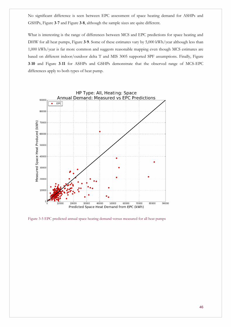
46
No significant difference is seen between EPC assessment of space heating demand for ASHPs and
GSHPs, Figure 3-7 and Figure 3-8, although the sample sizes are quite different.
What is interesting is the range of differences between MCS and EPC predictions for space heating and
DHW for all heat pumps, Figure 3-9. Some of these estimates vary by 5,000 kWh/year although less than
1,000 kWh/year is far more common and suggests reasonable mapping even though MCS estimates are
based on different indoor/outdoor delta T and MIS 3005 supported SPF assumptions. Finally, Figure
3-10 and Figure 3-11 for ASHPs and GSHPs demonstrate that the observed range of MCS-EPC
differences apply to both types of heat pump.
Figure 3-5 EPC predicted annual space heating demand versus measured for all heat pumps
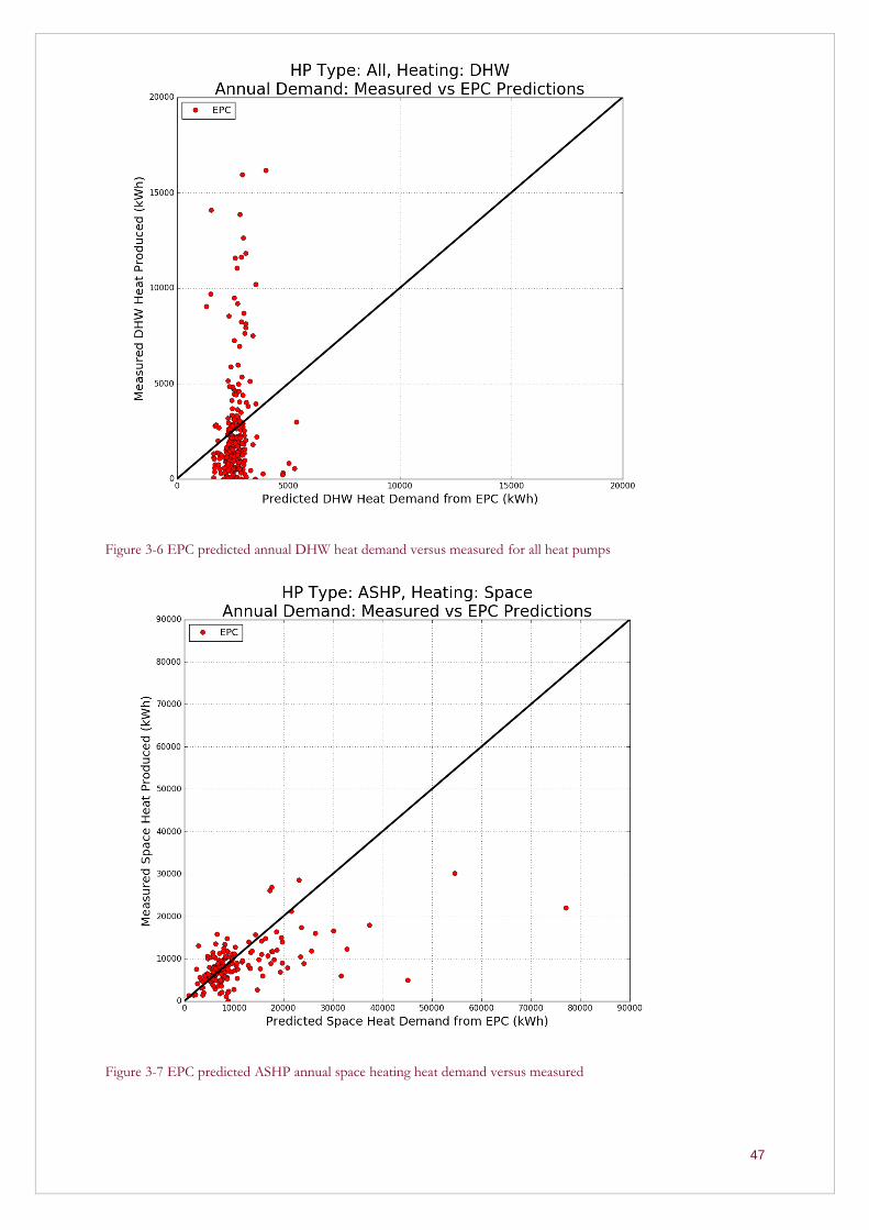
47
Figure 3-6 EPC predicted annual DHW heat demand versus measured for all heat pumps
Figure 3-7 EPC predicted ASHP annual space heating heat demand versus measured
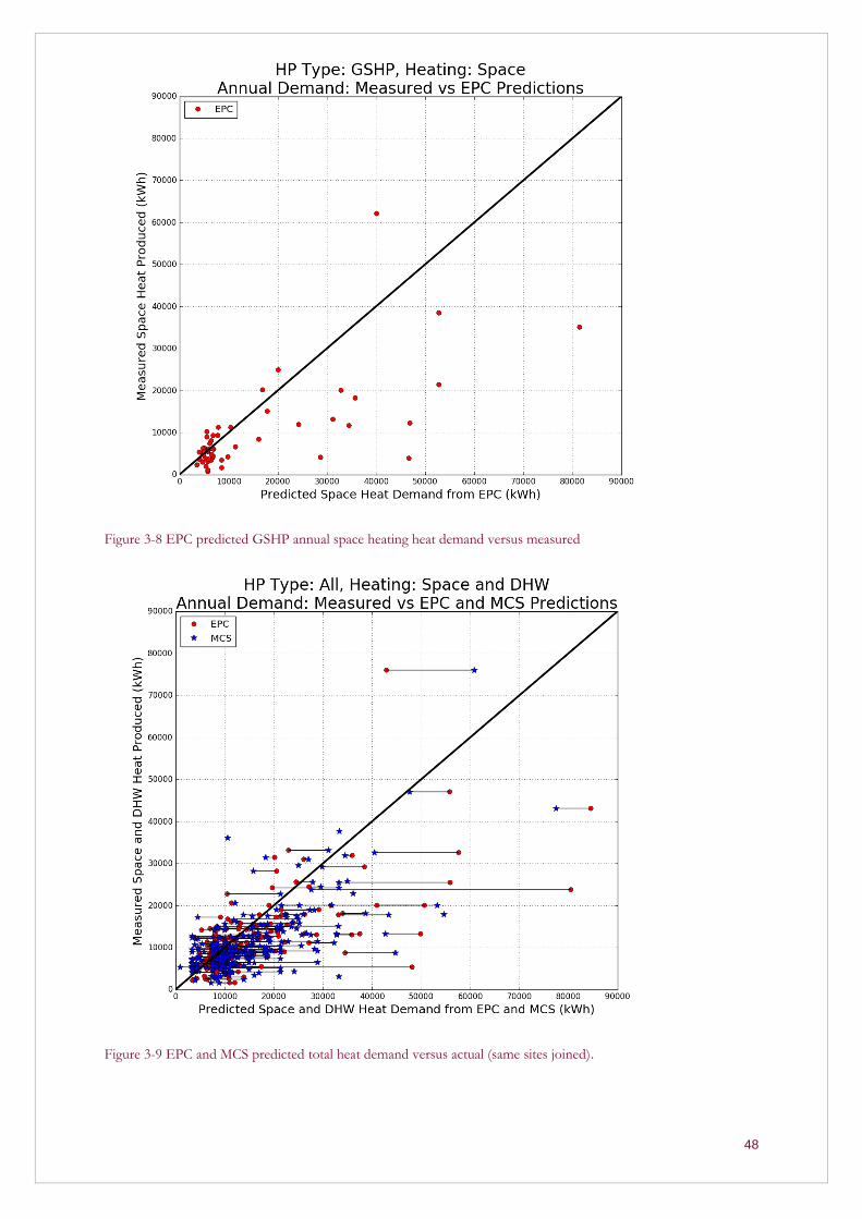
48
Figure 3-8 EPC predicted GSHP annual space heating heat demand versus measured
Figure 3-9 EPC and MCS predicted total heat demand versus actual (same sites joined).
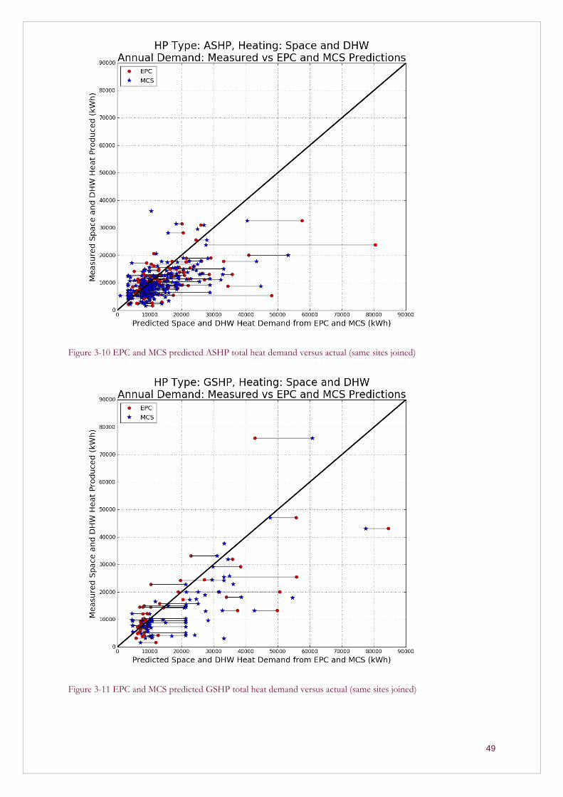
49
Figure 3-10 EPC and MCS predicted ASHP total heat demand versus actual (same sites joined)
Figure 3-11 EPC and MCS predicted GSHP total heat demand versus actual (same sites joined)
50
When reviewing Figures 3-5 to 3-11 it is worth considering the literature regarding EPCs and in particular
the variation in assessment between individual assessors (DECC, 2014b: iii):
“There was a lack of consistency in the data, results and advice generated by different assessors
for the same property. There was significant variation in the EPC and OA [Occupancy
Assessment] results produced by the different assessments conducted at individual properties.
The range of EPC ratings spanned at least two EPC bands for almost two thirds of the dwellings
analysed. The analysis found many differences in the values recorded for key input variables at
the same property. Input variation was observed with EPCs, particularly for total floor area and
the energy efficiency rating of building fabric and technologies. The variation in the inputs to the
EPC process contributed to the EPC rating varying by, on average, 11 points in each dwelling.”
Conclusion
Measured annual heat generated vs EPC and installers’ estimates: individual sites may have been affected
by small amounts of missing heat data. There is a systematic over-estimate of heat due to calibration of
sensors for water rather than glycol. This does not influence the conclusion that, for the period of data
examined, the EPC and installers’ estimates of annual heat demand are higher than the measured heat
produced.
The comparison of actual energy use with its calculated value, whether through MIS 3005 or EPC
procedures, is complicated by a range of factors that include the actual annual weather conditions, real as
opposed to ‘likely’ heating system efficiency, occupation pattern and comfort requirements. The graphical
analysis of both MIS and EPC estimates indicates a range of variables that are currently poorly expressed
in the calculations. Even for those installer companies that fully understand the role of likely SPF and
annual degree days, it is unlikely that the calculated results will provide anything other than a broad
estimate of annual energy use.
51
Do systems sterilise the hot water tank for legionella control? If so, how 4
often?
Sterilisation
The maximum outlet temperature of a heat pump is fixed by the manufacturer to ensure safe operation
and a minimum vapour compression cycle efficiency at high temperatures and pressures. For RHPP heat
pumps this temperature ranges between 50 and 65C and is dependent on the specific refrigerant mix.
For heat pumps with maximum condensing temperatures at or below 60C, the bulk temperature (the
mean or overall temperature) of the hot water cylinder will be below 60C for a variety of reasons
including cylinder stratification. Under these circumstances the stored hot water may fail to meet HSE
guidance on the protection from Legionnaires disease or legionella. A requirement for sterilisation of
DHW cylinders (or pasteurization as it is sometimes called) was introduced in MIS 3005 v 3.0 Section
4.2.5: “domestic hot water systems shall incorporate a means to prevent bacterial growth (including
Legionella bacteria). NOTE: Further guidance can be found within the Health and Safety Executive
Approved Code of Practice L8 document (HSE ACoP L8)”.
ACoP L8 is supported by HSG274 Part 2 which cites temperature as the most common method of
Legionella control: “It is recommended that hot water should be stored at 60°C and distributed so that it
reaches a temperature of 50°C within one minute at outlets.” However, this guidance is aimed primarily at
commercial hot water systems with either secondary returns (a pumped circulation pipe loop returning
hot water to the cylinder for continuous reheating), or trace heating (an electrical resistance tape attached
to the pipe where reheat is achieved by current flow in response to change in electrical resistance due to
any drop in temperature). It therefore should be noted that all HSG & ACoP’s refer to non-domestic
situations and very little specific advice is available for domestic applications.
Whilst secondary returns were observed in the trial case studies, most hot water systems comply with
water regulations, and therefore indirectly with HSG274, by limiting the length of hot water draw off
pipework or ‘deadlegs’. Since under these conditions it is expected that outlet temperatures will reach
cylinder temperature within one minute, Legionella control is primarily by regular high temperature
sterilisation.
Sterilisation or pasteurisation is achieved by raising the cylinder water to over 60C. HSG274 (which
refers to commercial installations) states that: “Arrangements should therefore be made to heat the whole
water content of the calorifier, including that at the base, to a temperature of 60°C for one hour each
day.” However, a review of heat pump manufacturers’ literature identifies varying guidance on the
sterilisation process with temperatures ranging from 65C to 73C for between 30 and 90 minutes either
weekly or fortnightly.
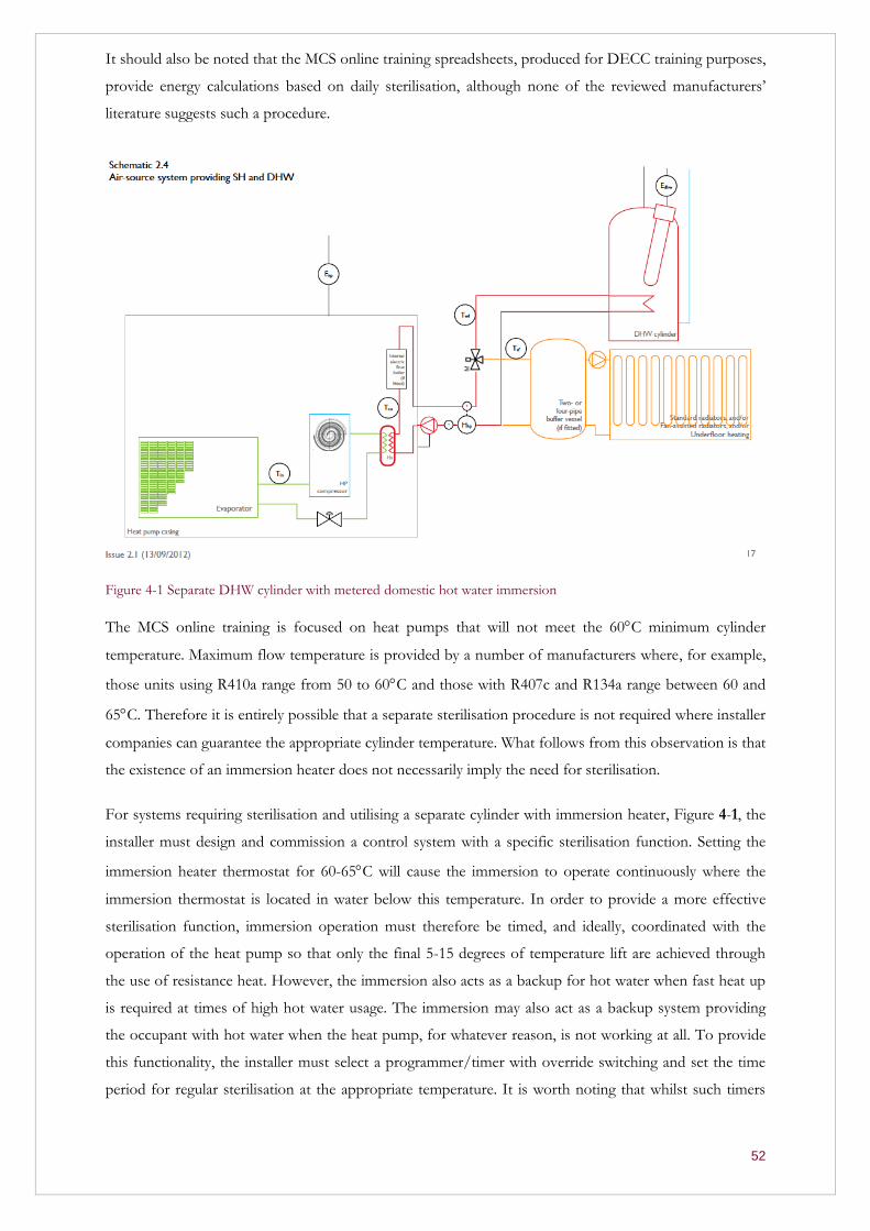
52
It should also be noted that the MCS online training spreadsheets, produced for DECC training purposes,
provide energy calculations based on daily sterilisation, although none of the reviewed manufacturers’
literature suggests such a procedure.
Figure 4-1 Separate DHW cylinder with metered domestic hot water immersion
The MCS online training is focused on heat pumps that will not meet the 60C minimum cylinder
temperature. Maximum flow temperature is provided by a number of manufacturers where, for example,
those units using R410a range from 50 to 60C and those with R407c and R134a range between 60 and
65C. Therefore it is entirely possible that a separate sterilisation procedure is not required where installer
companies can guarantee the appropriate cylinder temperature. What follows from this observation is that
the existence of an immersion heater does not necessarily imply the need for sterilisation.
For systems requiring sterilisation and utilising a separate cylinder with immersion heater, Figure 4-1, the
installer must design and commission a control system with a specific sterilisation function. Setting the
immersion heater thermostat for 60-65C will cause the immersion to operate continuously where the
immersion thermostat is located in water below this temperature. In order to provide a more effective
sterilisation function, immersion operation must therefore be timed, and ideally, coordinated with the
operation of the heat pump so that only the final 5-15 degrees of temperature lift are achieved through
the use of resistance heat. However, the immersion also acts as a backup for hot water when fast heat up
is required at times of high hot water usage. The immersion may also act as a backup system providing
the occupant with hot water when the heat pump, for whatever reason, is not working at all. To provide
this functionality, the installer must select a programmer/timer with override switching and set the time
period for regular sterilisation at the appropriate temperature. It is worth noting that whilst such timers

53
are available, they are not required for either gas or oil fired central heating where cylinder temperatures
above 60C may be achieved simply through setting the boiler thermostat; the immersion operates
(normally at 60-65C) only when required by the occupants. Heat pump installations may therefore
exhibit additional complexity with respect to DHW controls and their commissioning.
Recognising the potential for an automated legionella function, some manufacturers provide a controller
with these functions, either with factory default sterilisation, generally either weekly or fortnightly
operation, or as an option to be set during commissioning.
Analysis methodology
Cylinder temperatures were not monitored during the RHPP trials so analysis of sterilisation cannot be by
direct cylinder temperature measurement and must be inferred from immersion operating pattern.
Additionally, an installation with an immersion heater does not necessarily imply the need for sterilisation.
For example, for heat pumps capable of up to 65C flow temperature the immersion provides a back up
rather than sterilisation role. The analysis of sterilisation for this report is based on the following
understanding. Sterilisation of the hot water cylinder contents by heating the water to high temperatures
can be achieved in a number of ways:
The heat pump could provide all the heat.
The heat pump could start heating until it reaches its maximum temperature limit and either an
integrated booster through-flow heater or an immersion heater could be used to bring the water
temperature up to the required level.
The heat pump may not be used at all and the through-flow booster heater or the immersion
heater could be used.
In this section we have focused on the use of the separately metered immersion heater as this has a very
clear signal in the data. A regular and prolonged signal from the electrical meter to the immersion heater
may be assumed to represent sterilisation.
The immersion heater electricity use is recorded as Edhw every 2 minutes in Watthours (Wh). During a
sterilisation cycle, the control system will maintain the cylinder at the required temperature for an
extended period of time (up to an hour)25. For a lot of systems these intense heating episodes appear at
regular intervals, depending on how the systems were commissioned and operated. To detect a signal of a
high intensity heating episode, the data was scanned for any periods where the Edhw electricity use in a 1
hour period exceeded a threshold of 1.0 kW averaged over the hour26,27. This threshold level was chosen
25 For well insulated cylinders, with temperature decay rates of 1K per hour or less, it is unlikely that there would be any cycling,
once pasteurisation temperature had been reached. 26 Edhw was summed as 30 x 2min Wh samples in each hour. If that was more than 1000 Wh or 1kWh it was taken as a high
intensity episode. How this was distributed within the hour was not evaluated so, at one extreme, there could have been a 30 kW immersion working for the first 2 minutes and then nothing else, or at the other, a 1kW immersion working continuously for an hour. In this context the term "power" could be misleading. It is the average power over the hour.

54
as it is above the normal hourly use of the immersion heater in most systems where the cylinder is heated
to a lower temperature and stops once the set temperature has been reached. A histogram is then made of
the time interval in days between successive high intensity heating episodes. The peak frequency is
obvious in most cases where a regular schedule has been used. When sterilisation is not occurring via the
immersion heater or not at all the histogram shows a large peak at zero time interval.
Analysis results
The immersion heater frequency for each site is plotted showing a range of schedules in the sample,
Figure 4-2.
Figure 4-2 Assessment of apparent immersion frequency
Of the 417 heat pumps in Sample B2, monitoring schematics indicate that 288 should have monitored
DHW immersion. However, the data showed that only 220 of these sites actually used the immersion (ie
the sum of their immersion electricity consumption > 0). To these 220 sites, an algorithm was applied to
determine whether their immersion use followed a regular pattern, which may indicate that it was related
to sterilisation, and if there was a regular pattern, what its frequency was. 60% of sites with immersion
showed no pattern (therefore showing sporadic immersion use instead). These are plotted at x = 0 on
Figure 4.2. 40% of sites with immersion showed a regular pattern although sterilisation at these intervals
appears unlikely with intervals such as 3, 8 and 15 days. A sterilisation regime would be expected to occur
27 This is sufficient to raise the temperature of 120 litres of water by approximately 7K, enough to achieve a temperature of over
60C for a cylinder in which a temperature of 55C had already been achieved by the use of the heat pump.

55
either daily, weekly or fortnightly. The analysis shows that 28% of sites showed this ‘expected frequency’
of use.
Conclusion
Sterilisation analysis is based on electricity data. Electricity monitoring is generally of high quality; we do
not consider that metering errors will have had any effect on the conclusion that between ⅓ and ¼ of the
sites examined show regular patterns of immersion.
A protection regime against the build up of legionella bacteria is only required where cylinder
temperatures are below 60C. Importantly, since DHW temperature was not monitored, compliance with
HSE guidance cannot be confirmed and must necessarily be inferred by such methods as time-series data
analysis. RAPID-HPC recognize the limitations of such an approach and suggest that the assessment of
compliance be taken as provisional. Where we expect legionella sterilisation frequency to be daily, weekly
or fortnightly, we conclude that between a quarter and one third of RHPP installations with a metered
immersion heater exhibit a pattern of operation broadly consistent with MIS 3005 legionella criteria.
56
What are the actual flow temperatures at the MCS 3005 design temperature 5
conditions? What Heat Emitter Guide28 star rating would apply, based on the
actual flow temperatures?
Introduction
The installation ‘star rating’ and ‘likely space heating SPF’ would have been assessed from the planned
design flow temperature to radiators and underfloor heating but will depend on the individual heat
pump’s control type and settings. Heat pumps are controlled by a thermistor attached to the flow or to
the return. For systems controlled on return temperature, a low return temperature implies a high heat
flow from the radiators due to significant temperature difference between radiators and room air
temperature, whereas a high return indicates that the room is at or near design temperature. Variable
compressor heat pumps are able to adjust compression, and thus indirectly control flow temperature
from the condenser heat exchanger, to provide space heating water at the design flow temperature.
However for fixed speed units, where the water is either below or above set point, control is limited to
on/off. Final room control is commonly by thermostatic radiator valve or room thermostat. The rate of
heat transfer from the condenser to the heating circuit is dependent on condenser temperature, the return
temperature and mass flow rate. For return temperature control, this results in uncontrolled flow
temperatures which may rise to the maximum heat pump output temperature with implications for
Carnot efficiency. Such systems often allow the installer to set a maximum flow temperature to ensure a
minimum SPF and compliance with HEG design criteria. Thus it is common for heat pumps to provide
the option for two maximum set points, one for domestic hot water - controlled in conjunction with the
cylinder thermostat signal, and a lower setting for space heating controlled through the room thermostat
signal.
Some manufacturers use a ‘degree minute’ control function that integrates the temperature difference
between return temperature and its set point. At a pre-specified negative degree-minute summation an
electrical heater may be operated to provide a boost to the water temperature to speed up the heating
process. Many such systems also have a default maximum output temperature (such as 60C) reflecting
the heat pump’s maximum temperature output which the installer should reset to reflect their design star
rating and their choice of HEG likely SPF.
In addition, many manufacturers offer weather compensation control where space heating water
temperature is adjusted in response to outdoor temperature resulting in a ‘heating curve’ that adjusts the
flow temperature. As outdoor temperatures rise, the building requires less heat to achieve room
temperatures and emitter water temperature is reduced resulting, in theory, in a higher Carnot efficiency.
28 MCS 021: http://www.microgenerationcertification.org/mcs-standards/installer-standards
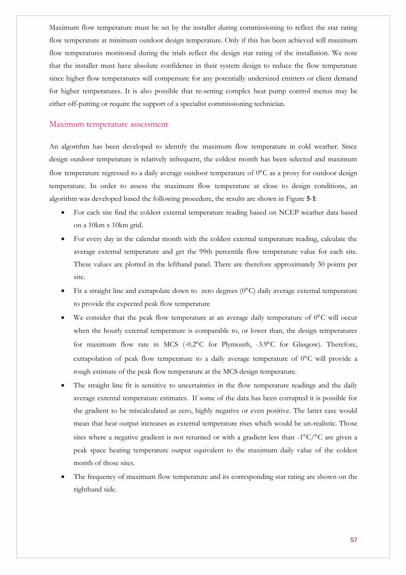
57
Maximum flow temperature must be set by the installer during commissioning to reflect the star rating
flow temperature at minimum outdoor design temperature. Only if this has been achieved will maximum
flow temperatures monitored during the trials reflect the design star rating of the installation. We note
that the installer must have absolute confidence in their system design to reduce the flow temperature
since higher flow temperatures will compensate for any potentially undersized emitters or client demand
for higher temperatures. It is also possible that re-setting complex heat pump control menus may be
either off-putting or require the support of a specialist commissioning technician.
Maximum temperature assessment
An algorithm has been developed to identify the maximum flow temperature in cold weather. Since
design outdoor temperature is relatively infrequent, the coldest month has been selected and maximum
flow temperature regressed to a daily average outdoor temperature of 0C as a proxy for outdoor design
temperature. In order to assess the maximum flow temperature at close to design conditions, an
algorithm was developed based the following procedure, the results are shown in Figure 5-1:
For each site find the coldest external temperature reading based on NCEP weather data based
on a 10km x 10km grid.
For every day in the calendar month with the coldest external temperature reading, calculate the
average external temperature and get the 99th percentile flow temperature value for each site.
These values are plotted in the lefthand panel. There are therefore approximately 30 points per
site.
Fit a straight line and extrapolate down to zero degrees (0C) daily average external temperature
to provide the expected peak flow temperature
We consider that the peak flow temperature at an average daily temperature of 0C will occur
when the hourly external temperature is comparable to, or lower than, the design temperatures
for maximum flow rate in MCS (-0.2C for Plymouth, -3.9C for Glasgow). Therefore,
extrapolation of peak flow temperature to a daily average temperature of 0C will provide a
rough estimate of the peak flow temperature at the MCS design temperature.
The straight line fit is sensitive to uncertainties in the flow temperature readings and the daily
average external temperature estimates. If some of the data has been corrupted it is possible for
the gradient to be miscalculated as zero, highly negative or even positive. The latter case would
mean that heat output increases as external temperature rises which would be un-realistic. Those
sites where a negative gradient is not returned or with a gradient less than -1C/C are given a
peak space heating temperature output equivalent to the maximum daily value of the coldest
month of those sites.
The frequency of maximum flow temperature and its corresponding star rating are shown on the
righthand side.
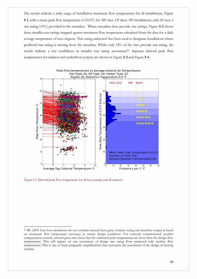
58
The results indicate a wide range of installation maximum flow temperatures for all installations, Figure
5-1, with a mean peak flow temperature of 43.6C for 189 sites. Of these 189 installations, only 26 have a
star rating (14%) provided in the metadata. Where metadata does provide star ratings, Figure 5-2 shows
these installer star ratings mapped against maximum flow temperature calculated from the data for a daily
average temperature of zero degrees. ‘Star rating unknown’ has been used to designate installations where
predicted star rating is missing from the metadata. Whilst only 14% of the sites provide star rating, the
results indicate a low confidence in installer star rating assessment29. Separate derived peak flow
temperatures for radiator and underfloor systems are shown in Figure 5-3 and Figure 5-4.
Figure 5-1 Derived peak flow temperature for all heat pumps and all emitters
29 BS 12831 heat loss calculations do not consider internal heat gains. Emitter sizing and therefore output is based on maximum flow temperature necessary to ensure design conditions. For correctly commissioned weather compensation control, internal gains may mean that the estimated peak temperatures are lower than the design flow temperatures. This will impact on our assessment of design star rating from projected cold weather flow temperatures. This is one of many pragmatic simplifications that surrounds the assessment of the design of heating systems.
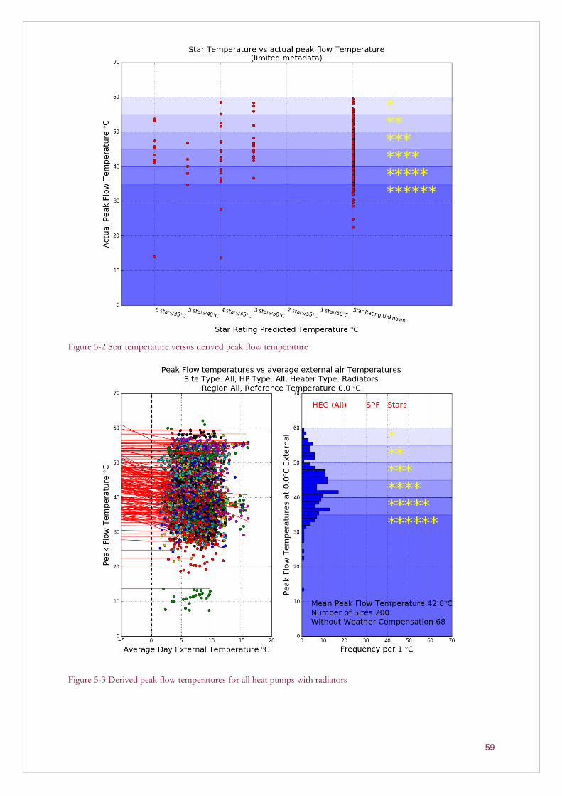
59
Figure 5-2 Star temperature versus derived peak flow temperature
Figure 5-3 Derived peak flow temperatures for all heat pumps with radiators
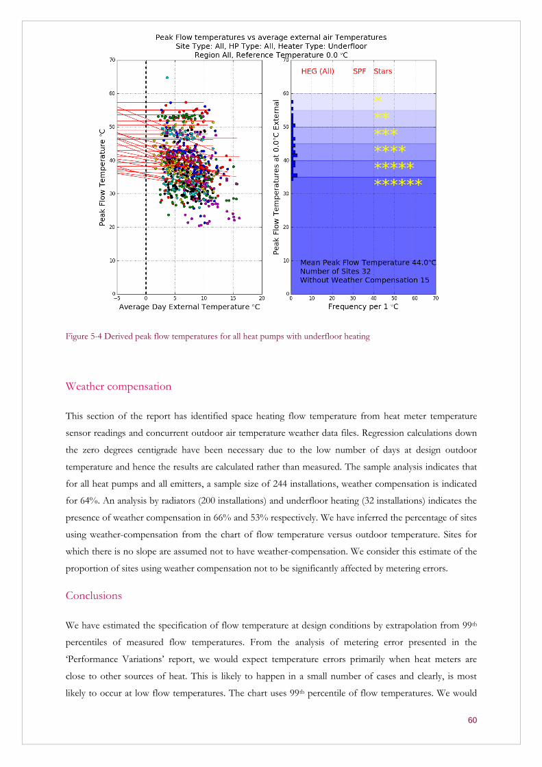
60
Figure 5-4 Derived peak flow temperatures for all heat pumps with underfloor heating
Weather compensation
This section of the report has identified space heating flow temperature from heat meter temperature
sensor readings and concurrent outdoor air temperature weather data files. Regression calculations down
the zero degrees centigrade have been necessary due to the low number of days at design outdoor
temperature and hence the results are calculated rather than measured. The sample analysis indicates that
for all heat pumps and all emitters, a sample size of 244 installations, weather compensation is indicated
for 64%. An analysis by radiators (200 installations) and underfloor heating (32 installations) indicates the
presence of weather compensation in 66% and 53% respectively. We have inferred the percentage of sites
using weather-compensation from the chart of flow temperature versus outdoor temperature. Sites for
which there is no slope are assumed not to have weather-compensation. We consider this estimate of the
proportion of sites using weather compensation not to be significantly affected by metering errors.
Conclusions
We have estimated the specification of flow temperature at design conditions by extrapolation from 99th
percentiles of measured flow temperatures. From the analysis of metering error presented in the
‘Performance Variations’ report, we would expect temperature errors primarily when heat meters are
close to other sources of heat. This is likely to happen in a small number of cases and clearly, is most
likely to occur at low flow temperatures. The chart uses 99th percentile of flow temperatures. We would

61
therefore not expect these estimates to be unduely affected by metering error but may be influenced
where monitored temperatures are taken from strap-on sensors.
A calculated mean peak temperature for radiators of around 43C indicates a general tendency to
maximise space heating SPF with 4 star installations. However, the analysis also indicates high
temperature flow regimes in radiator and, in particular, in underfloor heating systems. With regard to the
latter, underfloor heating in carpeted timber floors may require higher temperatures to ensure adequate
heat output (see footnote 2). It is apparent that heating temperatures could be better controlled in order
to benefit from Carnot performance. Finally, that there is little correlation between flow temperature and
installer assigned ‘star rating’ is perhaps understandable given that, in 2012 when use of the HEG became
obligatory, the terminology was entirely new to the heating industry.
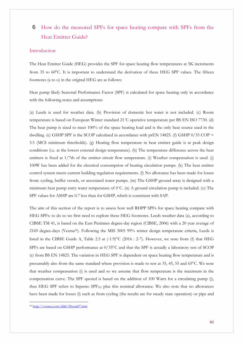
62
How do the measured SPFs for space heating compare with SPFs from the 6
Heat Emitter Guide?
Introduction
The Heat Emitter Guide (HEG) provides the SPF for space heating flow temperatures at 5K increments
from 35 to 60C. It is important to understand the derivation of these HEG SPF values. The fifteen
footnotes (a to o) in the original HEG are as follows:
Heat pump likely Seasonal Performance Factor (SPF) is calculated for space heating only in accordance
with the following notes and assumptions:
(a) Leeds is used for weather data. (b) Provision of domestic hot water is not included. (c) Room
temperature is based on European Winter standard 21˚C operative temperature per BS EN ISO 7730. (d)
The heat pump is sized to meet 100% of the space heating load and is the only heat source used in the
dwelling. (e) GSHP SPF is the SCOP calculated in accordance with prEN 14825. (f) GSHP 0/35 COP =
3.5 (MCS minimum thresholds). (g) Heating flow temperature in heat emitter guide is at peak design
conditions (i.e. at the lowest external design temperature). (h) The temperature difference across the heat
emitters is fixed at 1/7th of the emitter circuit flow temperature. (i) Weather compensation is used. (j)
100W has been added for the electrical consumption of heating circulation pumps. (k) The heat emitter
control system meets current building regulation requirements. (l) No allowance has been made for losses
from: cycling, buffer vessels, or associated water pumps. (m) The GSHP ground array is designed with a
minimum heat pump entry water temperature of 0˚C. (n) A ground circulation pump is included. (o) The
SPF values for ASHP are 0.7 less than for GSHP, which is consistent with SAP.
The aim of this section of the report is to assess how well RHPP SPFs for space heating compare with
HEG SPFs: to do so we first need to explore these HEG footnotes. Leeds weather data (a), according to
CIBSE TM 41, is based on the East Peninnes degree-day region (CIBSE, 2006) with a 20 year average of
2169 degree-days (Vesma30). Following the MIS 3005 99% winter design temperature criteria, Leeds is
listed in the CIBSE Guide A, Table 2.5 at (-1.9)C (2016 : 2-7). However, we note from (f) that HEG
SPFs are based on GSHP performance at 0/35C and that the SPF is actually a laboratory test of SCOP
(e) from BS EN 14825. The variation in HEG SPF is dependent on space heating flow temperature and is
presumably also from the same standard where provision is made to test at 35, 45, 55 and 65C. We note
that weather compensation (i) is used and so we assume that flow temperature is the maximum in the
compensation curve. The SPF quoted is based on the addition of 100 Watts for a circulating pump (j),
thus HEG SPF refers to Sepemo SPFH2 plus this nominal allowance. We also note that no allowances
have been made for losses (l) such as from cycling (the results are for steady state operation) or pipe and
30 http://vesma.com/ddd/20year07.htm

63
vessel losses. Thus for GSHPs we would expect RHPP SPFs to be somewhat less than those provided in
the HEG. HEG SPF values for ASHPs (o) are derived from GSHP SPF results by the simple subtraction
of 0.7. We may note from the RHPP Detailed Report (RAPID-HPC, 2016) that the difference between
ground and air source heat pumps at SPFH2 in the three samples is an average of 0.33.
Derived maximum flow temperatures
The HEG assumes that SPF is a function of flow temperature. For comparison with RHPP SPFH2 it is
necessary to identify maximum space heating flow temperatures and the HEG SPF associated with each
system for that temperature. Graphs are provided for all GSHPS and ASHPs where maximum flow
temperature is plotted as described in Section 5.1. For each site, SPFH2 is then compared with the HEG
SPF.
Figure 6-1 Derived peak flow temperatures for GSHPs
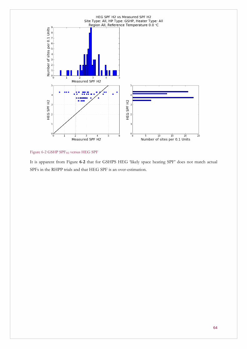
64
Figure 6-2 GSHP SPFH2 versus HEG SPF
It is apparent from Figure 6-2 that for GSHPS HEG ‘likely space heating SPF’ does not match actual
SPFs in the RHPP trials and that HEG SPF is an over-estimation.
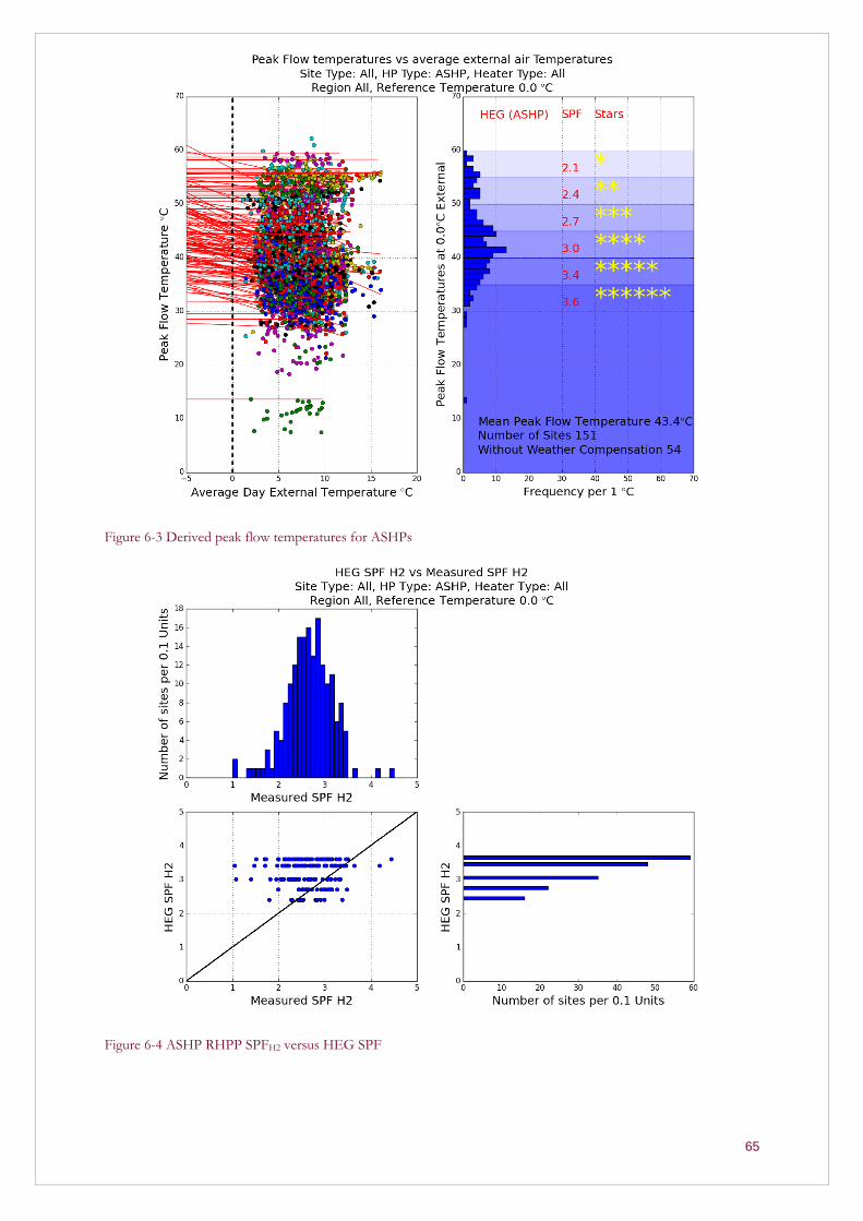
65
Figure 6-3 Derived peak flow temperatures for ASHPs
Figure 6-4 ASHP RHPP SPFH2 versus HEG SPF

66
HEG SPFs for ASHPs, are, in comparison to HEG SPFs for GSHPs, more closely matched to measured
RHPP SPFs although clearly HEG SPF is predominantly higher than trial SPF. Statistical comparison
between measured and HEG SPF is provided in Table 6–1.
SPF values ASHPs GSHPs
median measured SPFs 2.65 2.78
median HEG SPFs 3.40 4.10
IQR measured 0.64 0.64
IQR HEG 0.60 0.60 Table 6–1 Statistical analysis of measured and HEG SPF
Modelling of SPF as a function of load factor
Appendix D shows a comparison of modelled and measured SPFH2 as a function of load factor. The
modelling indicates that the wide variation observed in the results could, potentially, be the result of
parasitic electrical loads within the H2 boundary such as controls, inlet fans (ASHP) or ground loop
circulating pumps (GSHP).
Conclusion
As described in the ‘Performance Variations’ report, a range of metering errors can affect individual
estimates of SPFH2 with some causing an increase, others a decrease. There is a systematic over-estimate
of heat flow of 4 - 7% caused by calibration of heat meters for water instead of glycol, which one would
expect to find in all hydronic split ASHPs and externally located GSHPs. However, this margin of error
would not be expected to greatly affect the overall result found here, namely that calculated space heating
efficiency does not correlate with the expected SPFH2 from the MCS Heat Emitter Guide for the heat
pumps examined.
The design assessment of ‘likely space heating SPF’ is required to calculate annual energy costs for both
air and ground source heat pumps. However, for GSHPs, the initial assessment of SPF is integral to
ground loop sizing and therefore its accurate prediction is critical for ensuring that the system can extract
adequate heat from the ground. The comparison of HEG ‘likely space heating SPF’ with RHPP field trial
SPF provides some justification for a change in SPF assessment methodology. Compliance with ErP
requirements has resulted in the removal of ‘likely space heating SPF’ from the latest version of the HEG
and its replacement with individual heat pump laboratory test results for seasonal coefficient of
performance (SCOP) at a series of space heating flow temperatures and available from the MCS Product

67
search database31. Mapping individual manufacturers’ heat pump SCOP with trial SPF has not been
carried out for this report.
31 MCS Product search database: http://www.microgenerationcertification.org/consumers/product-search
68
References
BRE, 2005. The Government’s Standard Assessment Procedure for Energy Rating of Dwellings: 2005
edition, Watford: BRE on behalf of DECC. http://projects.bre.co.uk/sap2005/
BS EN 12831:2003. Heating systems in buildings. Method for calculation of the design heat load
BS EN 14511:2007. Air conditioners, liquid chilling packages and heat pumps with electrically driven
compressors for space heating and cooling: - Part 1: Terms and definitions - Part 2: Test conditions - Part
3: Test methods - Part 4: Requirements. BSI
BS EN 14825:2013. Air conditioners, liquid chilling packages and heat pumps, with electrically driven
compressors, for space heating and cooling. Testing and rating at part load conditions and calculation of
seasonal performance
BS EN 16147:2011. Heat pumps with electrically driven compressors. Testing and requirements for
marking of domestic hot water units
CIBSE, 2007. Domestic Heating Design Guide. CIBSE publications
DCLG, 2000. Approved document L1 Conservation of fuel and power – effective from 1 April 2002
DECC, 2009. Final Report: In-situ monitoring of efficiencies of condensing boilers and use of secondary
heating.
DECC, 2010. Renewable Energy Statistics, Data Sources and Methodologies.
https://www.gov.uk/government/publications/renewable-energy-statistics-data-sources-and-
methodologies
DECC, 2014a. RHI and RHPP deployment data: November 2014.
https://www.gov.uk/government/statistics/rhi-and-rhpp-deployment-data-november-2014
DECC, 2014b. Green Deal Assessment Mystery Shopping Research: Mystery shopping of customer
experiences of Green Deal assessments with 48 households and analysis of variability across Green Deal
Assessment Reports of 29 properties. London: DECC.
https://www.gov.uk/government/uploads/system/uploads/attachment_data/file/388197/Green_Deal_
Assessment_Mystery_Shopping_FINAL_PUBLISHED.pdf .
Dunbabin, P., Charlick, H., & Green, R., 2013. Detailed analysis from the second phase of the Energy
Saving Trust's heat pump field trial. London: DECC.
https://www.gov.uk/government/uploads/system/uploads/attachment_data/file/225825/analysis_data
_second_phase_est_heat_pump_field_trials.pdf

69
Dunbabin, P., & Wickins, C., 2012. Detailed analysis from the first phase of the Energy Saving Trust’s
heat pump field trial: Evidence to support the revision of the MCS Installer Standard MIS 3005 Issue 3.1.
London: DECC.
https://www.gov.uk/government/uploads/system/uploads/attachment_data/file/48327/5045-heat-
pump-field-trials.pdf
EST, 2010. Getting warmer: a field trial of heat pumps.
http://www.heatpumps.org.uk/PdfFiles/TheEnergySavingTrust-
GettingWarmerAFieldTrialOfHeatPumps.pdf
European Commission, 2009a. Directive 2009/28/EC of the European Parliament and of the Council of
23 April 2009 on the promotion of the use of energy from renewable sources and amending and
subsequently repealing Directives 2001/77/EC and 2003/30/EC.
European Commission, 2009b. Directive 2009/28/EC of the European Parliament and of the Council of
21 October 2009 establishing a framework for the setting of ecodesign requirements for energy-related
products.
European Commission, 2013a. Establishing the guidelines for Member States on calculating renewable
energy from heat pumps from different heat pump technologies pursuant to Article 5 of Directive
2009/28/EC of the European Parliament and of the Council.
Gleeson, C. P., Lowe, R., 2013. Meta-analysis of European heat pump field trial efficiencies. Energy and
Buildings 66, 637–647. doi:10.1016/j.enbuild.2013.07.064
Hulme J. and Doran S, 2014. In-situ measurements of wall U-values in English housing
https://www.gov.uk/government/uploads/system/uploads/attachment_data/file/409428/In-situ_u-
values_final_report.pdf
Li, Francis G. N., Smith, A.Z.P., Biddulph, P., Hamilton, I.G., Lowe, R.J., Mavrogianni, A., Oikonomou,
E., Raslan, R., Stamp, S., Stone, A., Summerfield, A.J., Veitch, D., Gori, V. & Oreszczyn, T., 2014. Solid-
wall U-values: heat flux measurements compared with standard assumptions, Building Research and
Information, 43 (2) 238-252. http://dx.doi.org/10.1080/09613218.2014.967977
Moss, K. J., 2003. Heating and water services design in buildings. Spon
Orr, G., Lelyveld, T., Burton, S (2009) Insitu monitoring of efficiencies of condensing boilers and use of
secondary heating.
Pickup and Miles (1977) The performance of domestic wet heat heating systems in contemporary and
future housing, I.G.E. Communication 1041. J.I.G.E. 18 (6) 188-204, and reproduced in British Gas
(1979) Studies in Energy Efficiency in Buildings.

70
Riviere, A., Coevoet, M., Tran, C., Zottl, A., Nordman, R., 2011. D4.2. / D 3. 4 . Concept for evaluation
of SPF - Version 2.0 - A defined methodology for calculation of the seasonal performance factor and a
definition which devices of the system have to be included in this calculation: Air to air heat pumps.
https://ec.europa.eu/energy/intelligent/projects/sites/iee-projects/files/projects/documents/sepemo-
build_concept_for_evaluation_of_spf_for_hydronic_hps_en.pdf
Saha, S., et al. 2011, updated monthly. NCEP Climate Forecast System Version 2 (CFSv2) Selected
Hourly Time-Series Products. Research Data Archive at the National Center for Atmospheric Research,
Computational and Information Systems Laboratory. http://rda.ucar.edu/datasets/ds094.1/. Accessed
25/06/2015.
Wickins, C., 2014. Preliminary report on the Renewable Heat Premium Payment metering programme.
London: DECC.
https://www.gov.uk/government/uploads/system/uploads/attachment_data/file/276612/Preliminary_
Report_on_the_RHPP_metering_programme_2014-01-31.pdf
Wingfield, J., Miles-Shenton, D. & Bell, M., (2010) Performance of Cavity Wall Insulation: A Field Trial
Investigation Interim Report No.1 – Review of Project Progress & Interim Results, Report to EURISOL,
Leeds Metropolitan University, Leeds
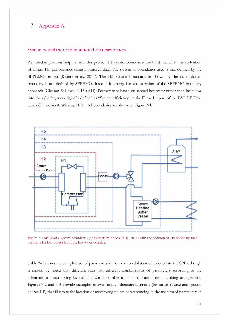
71
Appendix A 7
System boundaries and monitored data parameters
As noted in previous outputs from this project, HP system boundaries are fundamental to the evaluation
of annual HP performance using monitored data. The system of boundaries used is that defined by the
SEPEMO project (Riviere et al., 2011). The H5 System Boundary, as shown by the outer dotted
boundary is not defined by SEPEMO. Instead, it emerged as an extension of the SEPEMO boundary
approach (Gleeson & Lowe, 2013 : 641). Performance based on tapped hot water rather than heat flow
into the cylinder, was originally defined as “System efficiency” in the Phase I report of the EST HP Field
Trials (Dunbabin & Wickins, 2012). All boundaries are shown in Figure 7-1.
Figure 7-1 SEPEMO system boundaries (derived from Riviere et al., 2011) with the addition of H5 boundary that accounts for heat losses from the hot water cylinder.
Table 7–1 shows the complete set of parameters in the monitored data used to calculate the SPFs, though
it should be noted that different sites had different combinations of parameters according to the
schematic (or monitoring layout) that was applicable to that installation and plumbing arrangement.
Figures 7-2 and 7-3 provide examples of two simple schematic diagrams (for an air source and ground
source HP) that illustrate the location of monitoring points corresponding to the monitored parameters in

72
any given heat pump system. Full details of the monitoring programme, including the overall monitoring
philosophy and considerations of sensor resolution, can be found in the Preliminary Assessment report
(Wickins, 2014); a summary of this report will be published at the end of the project. Further details of
the heat metering have been provided in the form of private communications by Martin.
Parameter Description
Eb Electricity meter for whole system boost only
Edhw Electricity meter for domestic hot water (typically an immersion heater)
Ehp Electricity meter for the HP unit (may include a booster heater and
circulation pump)
Esp Electricity meter for boost to space heating only
Fhp Flow rate of water from HP (may be space heating only)
Fhw Flow rate of water to DHW cylinder
Hhp Heat meter from HP (may be space heating only)
Hhw Heat meter to DHW cylinder
Tco Temperature of refrigerant leaving the condenser
Tin For ASHP: Temperature of refrigerant leaving the evaporator
For GSHP: Temperature of ground loop water into the HP
Tsf Flow temperature of water to space heating
Twf Flow temperature of water to cylinder
Table 7–1 The complete set of parameters included in the monitored data
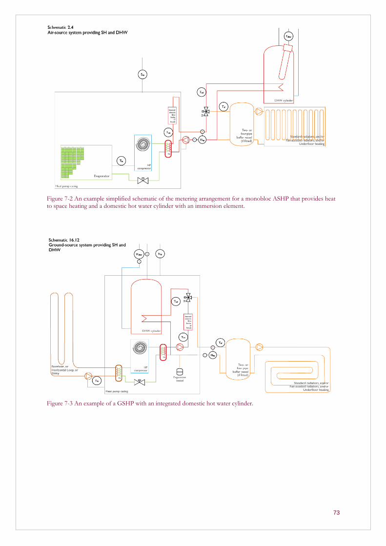
73
Figure 7-2 An example simplified schematic of the metering arrangement for a monobloc ASHP that provides heat to space heating and a domestic hot water cylinder with an immersion element.
Figure 7-3 An example of a GSHP with an integrated domestic hot water cylinder.
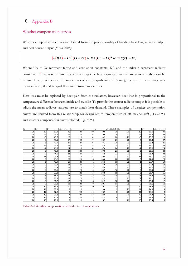
74
Appendix B 8
Weather compensation curves
Weather compensation curves are derived from the proportionality of building heat loss, radiator output
and heat source output (Moss 2003):
[𝜮(𝑼𝑨) + 𝑪𝒗](𝒕𝒔 − 𝒕𝒆) ∝ 𝑲𝑨(𝒕𝒎 − 𝒕𝒔)𝒏 ∝ ��𝑪(𝒕𝒇 − 𝒕𝒓)
Where UA + Cv represent fabric and ventilation constants; KA and the index n represent radiator
constants; mC represent mass flow rate and specific heat capacity. Since all are constants they can be
removed to provide ratios of temperatures where ts equals internal (space); te equals external; tm equals
mean radiator; tf and tr equal flow and return temperatures.
Heat loss must be replaced by heat gain from the radiators, however, heat loss is proportional to the
temperature difference between inside and outside. To provide the correct radiator output it is possible to
adjust the mean radiator temperature to match heat demand. Three examples of weather compensation
curves are derived from this relationship for design return temperatures of 50, 40 and 30C, Table 9-1
and weather compensation curves plotted, Figure 9-1.
Table 8–1 Weather compensation derived return temperatures
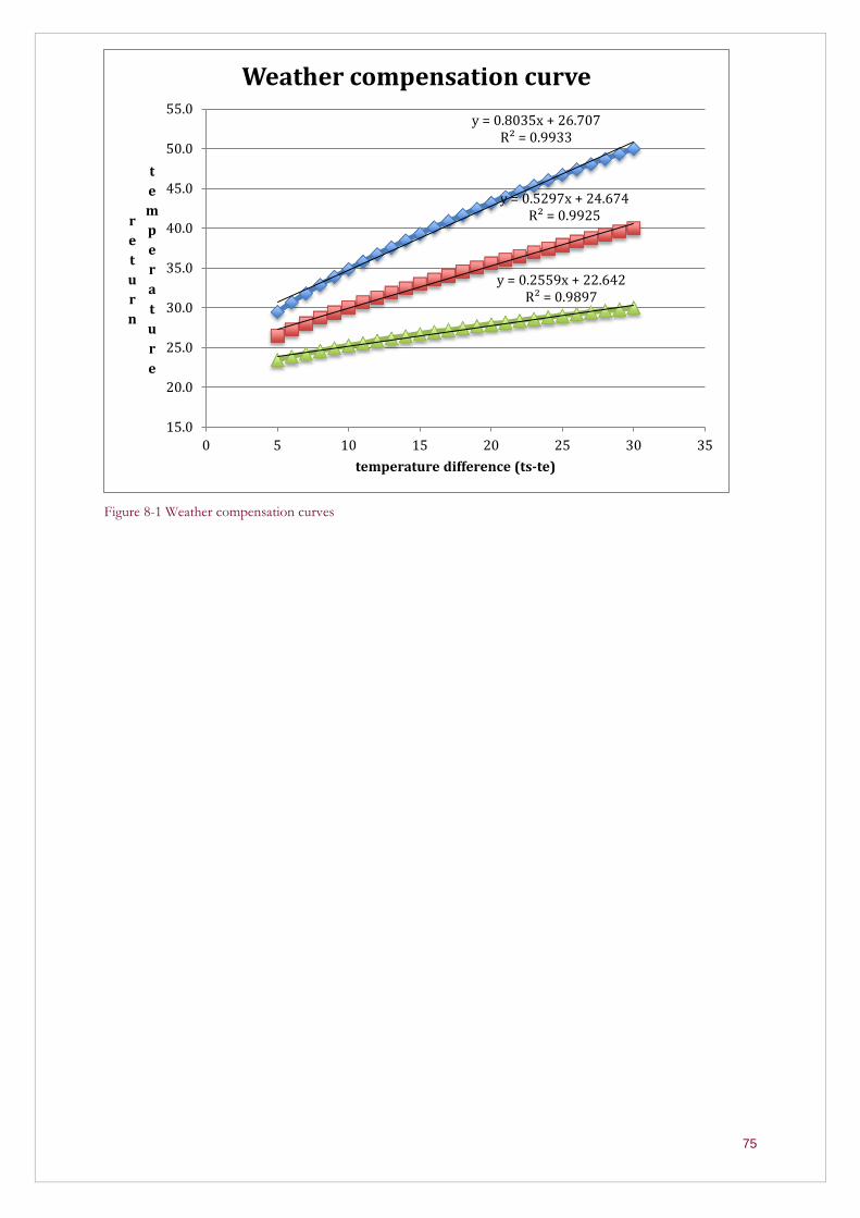
75
Figure 8-1 Weather compensation curves
y = 0.8035x + 26.707 R² = 0.9933
y = 0.5297x + 24.674 R² = 0.9925
y = 0.2559x + 22.642 R² = 0.9897
15.0
20.0
25.0
30.0
35.0
40.0
45.0
50.0
55.0
0 5 10 15 20 25 30 35
r
e
t
u
r
n
t
e
m
p
e
r
a
t
u
r
e
temperature difference (ts-te)
Weather compensation curve
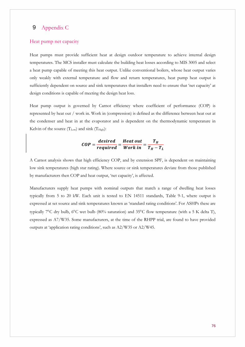
76
Appendix C 9
Heat pump net capacity
Heat pumps must provide sufficient heat at design outdoor temperature to achieve internal design
temperatures. The MCS installer must calculate the building heat losses according to MIS 3005 and select
a heat pump capable of meeting this heat output. Unlike conventional boilers, whose heat output varies
only weakly with external temperature and flow and return temperatures, heat pump heat output is
sufficiently dependent on source and sink temperatures that installers need to ensure that ‘net capacity’ at
design conditions is capable of meeting the design heat loss.
Heat pump output is governed by Carnot efficiency where coefficient of performance (COP) is
represented by heat out / work in. Work in (compression) is defined as the difference between heat out at
the condenser and heat in at the evaporator and is dependent on the thermodynamic temperature in
Kelvin of the source (TLow) and sink (THigh):
𝑪𝑶𝑷 =𝒅𝒆𝒔𝒊𝒓𝒆𝒅
𝒓𝒆𝒒𝒖𝒊𝒓𝒆𝒅=
𝑯𝒆𝒂𝒕 𝒐𝒖𝒕
𝑾𝒐𝒓𝒌 𝒊𝒏=
𝑻𝑯
𝑻𝑯 − 𝑻𝑳
A Carnot analysis shows that high efficiency COP, and by extension SPF, is dependent on maintaining
low sink temperatures (high star rating). Where source or sink temperatures deviate from those published
by manufacturers then COP and heat output, ‘net capacity’, is affected.
Manufacturers supply heat pumps with nominal outputs that match a range of dwelling heat losses
typically from 5 to 20 kW. Each unit is tested to EN 14511 standards, Table 9-1, where output is
expressed at set source and sink temperatures known as ‘standard rating conditions’. For ASHPs these are
typically 7C dry bulb, 6C wet bulb (80% saturation) and 35C flow temperature (with a 5 K delta T),
expressed as A7/W35. Some manufacturers, at the time of the RHPP trial, are found to have provided
outputs at ‘application rating conditions’, such as A2/W35 or A2/W45.
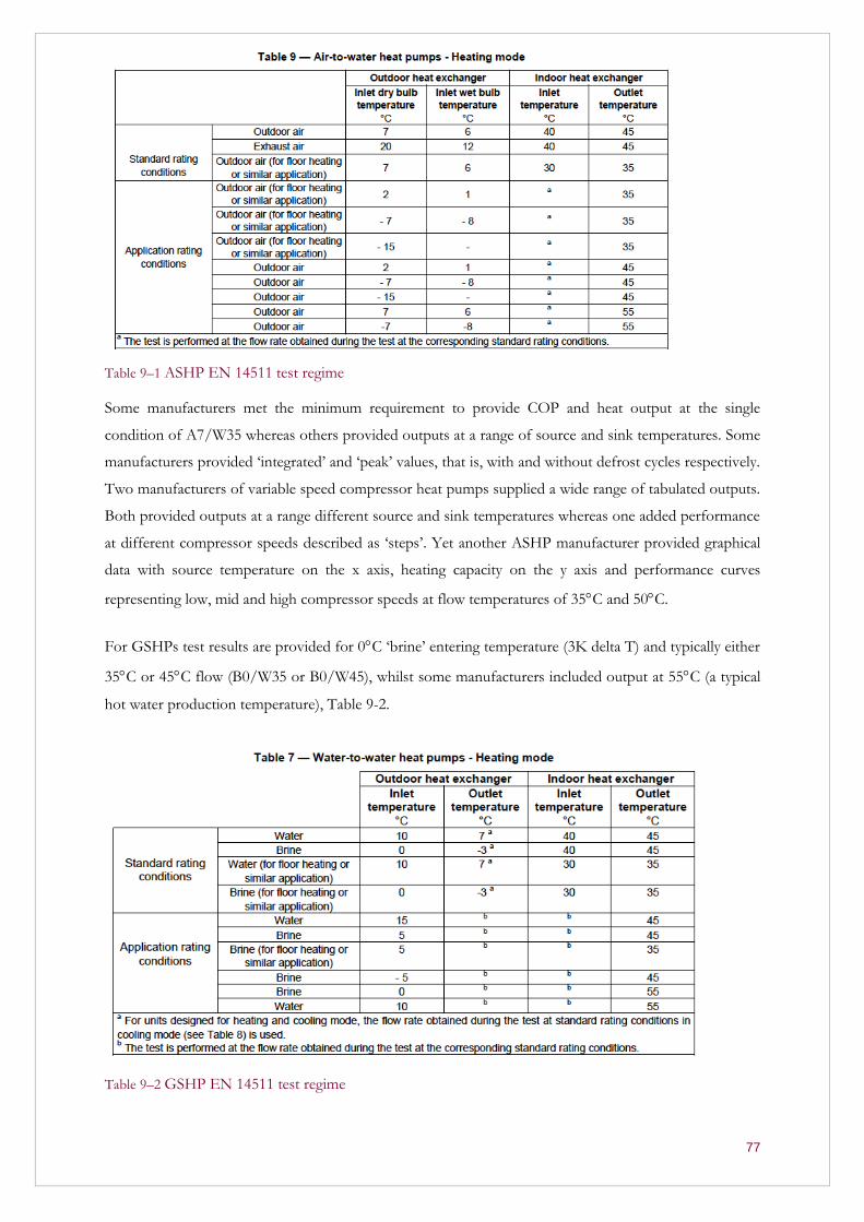
77
Table 9–1 ASHP EN 14511 test regime
Some manufacturers met the minimum requirement to provide COP and heat output at the single
condition of A7/W35 whereas others provided outputs at a range of source and sink temperatures. Some
manufacturers provided ‘integrated’ and ‘peak’ values, that is, with and without defrost cycles respectively.
Two manufacturers of variable speed compressor heat pumps supplied a wide range of tabulated outputs.
Both provided outputs at a range different source and sink temperatures whereas one added performance
at different compressor speeds described as ‘steps’. Yet another ASHP manufacturer provided graphical
data with source temperature on the x axis, heating capacity on the y axis and performance curves
representing low, mid and high compressor speeds at flow temperatures of 35C and 50C.
For GSHPs test results are provided for 0C ‘brine’ entering temperature (3K delta T) and typically either
35C or 45C flow (B0/W35 or B0/W45), whilst some manufacturers included output at 55C (a typical
hot water production temperature), Table 9-2.
Table 9–2 GSHP EN 14511 test regime
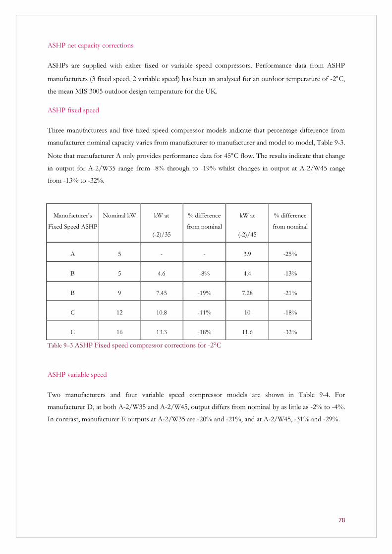
78
ASHP net capacity corrections
ASHPs are supplied with either fixed or variable speed compressors. Performance data from ASHP
manufacturers (3 fixed speed, 2 variable speed) has been an analysed for an outdoor temperature of -2C,
the mean MIS 3005 outdoor design temperature for the UK.
ASHP fixed speed
Three manufacturers and five fixed speed compressor models indicate that percentage difference from
manufacturer nominal capacity varies from manufacturer to manufacturer and model to model, Table 9-3.
Note that manufacturer A only provides performance data for 45C flow. The results indicate that change
in output for A-2/W35 range from -8% through to -19% whilst changes in output at A-2/W45 range
from -13% to -32%.
Manufacturer’s
Fixed Speed ASHP
Nominal kW kW at
(-2)/35
% difference
from nominal
kW at
(-2)/45
% difference
from nominal
A 5 - - 3.9 -25%
B 5 4.6 -8% 4.4 -13%
B 9 7.45 -19% 7.28 -21%
C 12 10.8 -11% 10 -18%
C 16 13.3 -18% 11.6 -32%
Table 9–3 ASHP Fixed speed compressor corrections for -2C
ASHP variable speed
Two manufacturers and four variable speed compressor models are shown in Table 9-4. For
manufacturer D, at both A-2/W35 and A-2/W45, output differs from nominal by as little as -2% to -4%.
In contrast, manufacturer E outputs at A-2/W35 are -20% and -21%, and at A-2/W45, -31% and -29%.
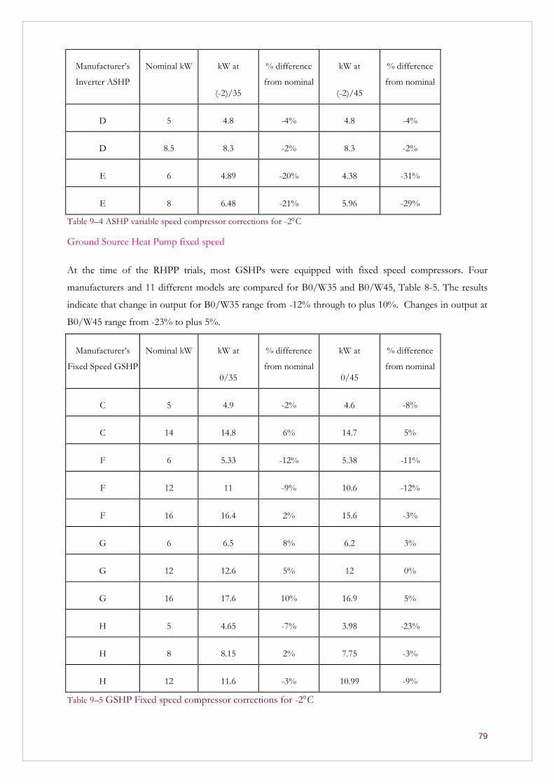
79
Manufacturer’s
Inverter ASHP
Nominal kW kW at
(-2)/35
% difference
from nominal
kW at
(-2)/45
% difference
from nominal
D 5 4.8 -4% 4.8 -4%
D 8.5 8.3 -2% 8.3 -2%
E 6 4.89 -20% 4.38 -31%
E 8 6.48 -21% 5.96 -29%
Table 9–4 ASHP variable speed compressor corrections for -2C
Ground Source Heat Pump fixed speed
At the time of the RHPP trials, most GSHPs were equipped with fixed speed compressors. Four
manufacturers and 11 different models are compared for B0/W35 and B0/W45, Table 8-5. The results
indicate that change in output for B0/W35 range from -12% through to plus 10%. Changes in output at
B0/W45 range from -23% to plus 5%.
Manufacturer’s
Fixed Speed GSHP
Nominal kW kW at
0/35
% difference
from nominal
kW at
0/45
% difference
from nominal
C 5 4.9 -2% 4.6 -8%
C 14 14.8 6% 14.7 5%
F 6 5.33 -12% 5.38 -11%
F 12 11 -9% 10.6 -12%
F 16 16.4 2% 15.6 -3%
G 6 6.5 8% 6.2 3%
G 12 12.6 5% 12 0%
G 16 17.6 10% 16.9 5%
H 5 4.65 -7% 3.98 -23%
H 8 8.15 2% 7.75 -3%
H 12 11.6 -3% 10.99 -9%
Table 9–5 GSHP Fixed speed compressor corrections for -2C

80
Conclusions
The impact of design conditions on badged capacity is shown to depend on both source and sink
temperatures. Fixed speed ASHPs most clearly show the negative impact of design temperature on
badged capacity. For variable speed ASHP the impact ranges from as little as -2% up to -30% depending
on the manufacturer. For GSHP fixed speed compressors the general pattern is a loss in capacity but one
that is again dependent on the make and model.
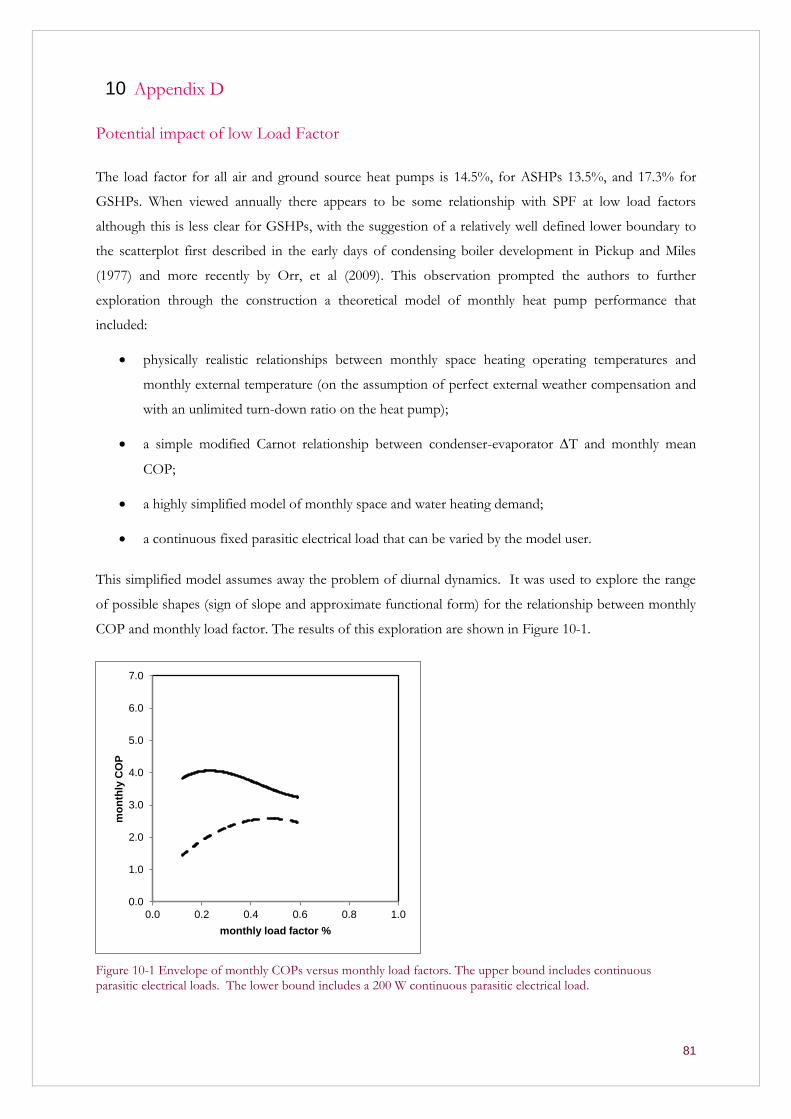
81
Appendix D 10
Potential impact of low Load Factor
The load factor for all air and ground source heat pumps is 14.5%, for ASHPs 13.5%, and 17.3% for
GSHPs. When viewed annually there appears to be some relationship with SPF at low load factors
although this is less clear for GSHPs, with the suggestion of a relatively well defined lower boundary to
the scatterplot first described in the early days of condensing boiler development in Pickup and Miles
(1977) and more recently by Orr, et al (2009). This observation prompted the authors to further
exploration through the construction a theoretical model of monthly heat pump performance that
included:
physically realistic relationships between monthly space heating operating temperatures and
monthly external temperature (on the assumption of perfect external weather compensation and
with an unlimited turn-down ratio on the heat pump);
a simple modified Carnot relationship between condenser-evaporator T and monthly mean
COP;
a highly simplified model of monthly space and water heating demand;
a continuous fixed parasitic electrical load that can be varied by the model user.
This simplified model assumes away the problem of diurnal dynamics. It was used to explore the range
of possible shapes (sign of slope and approximate functional form) for the relationship between monthly
COP and monthly load factor. The results of this exploration are shown in Figure 10-1.
Figure 10-1 Envelope of monthly COPs versus monthly load factors. The upper bound includes continuous parasitic electrical loads. The lower bound includes a 200 W continuous parasitic electrical load.
0.0
1.0
2.0
3.0
4.0
5.0
6.0
7.0
0.0 0.2 0.4 0.6 0.8 1.0
mo
nth
ly C
OP
monthly load factor %
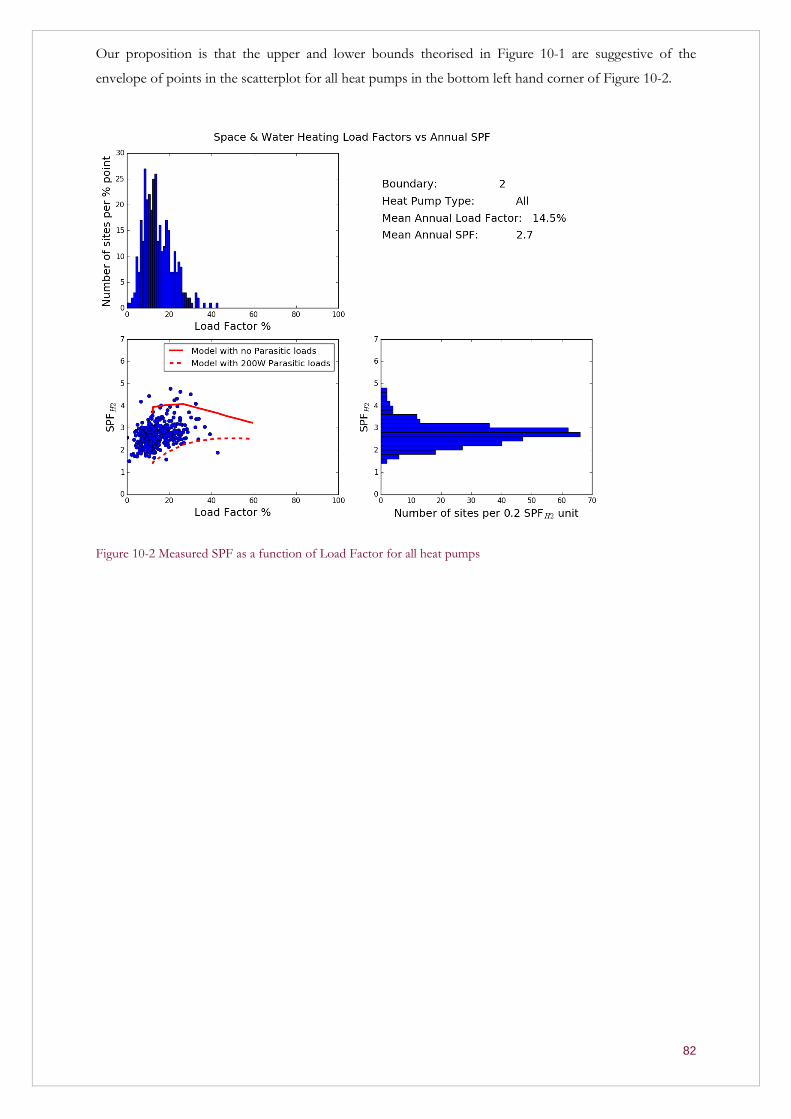
82
Our proposition is that the upper and lower bounds theorised in Figure 10-1 are suggestive of the
envelope of points in the scatterplot for all heat pumps in the bottom left hand corner of Figure 10-2.
Figure 10-2 Measured SPF as a function of Load Factor for all heat pumps
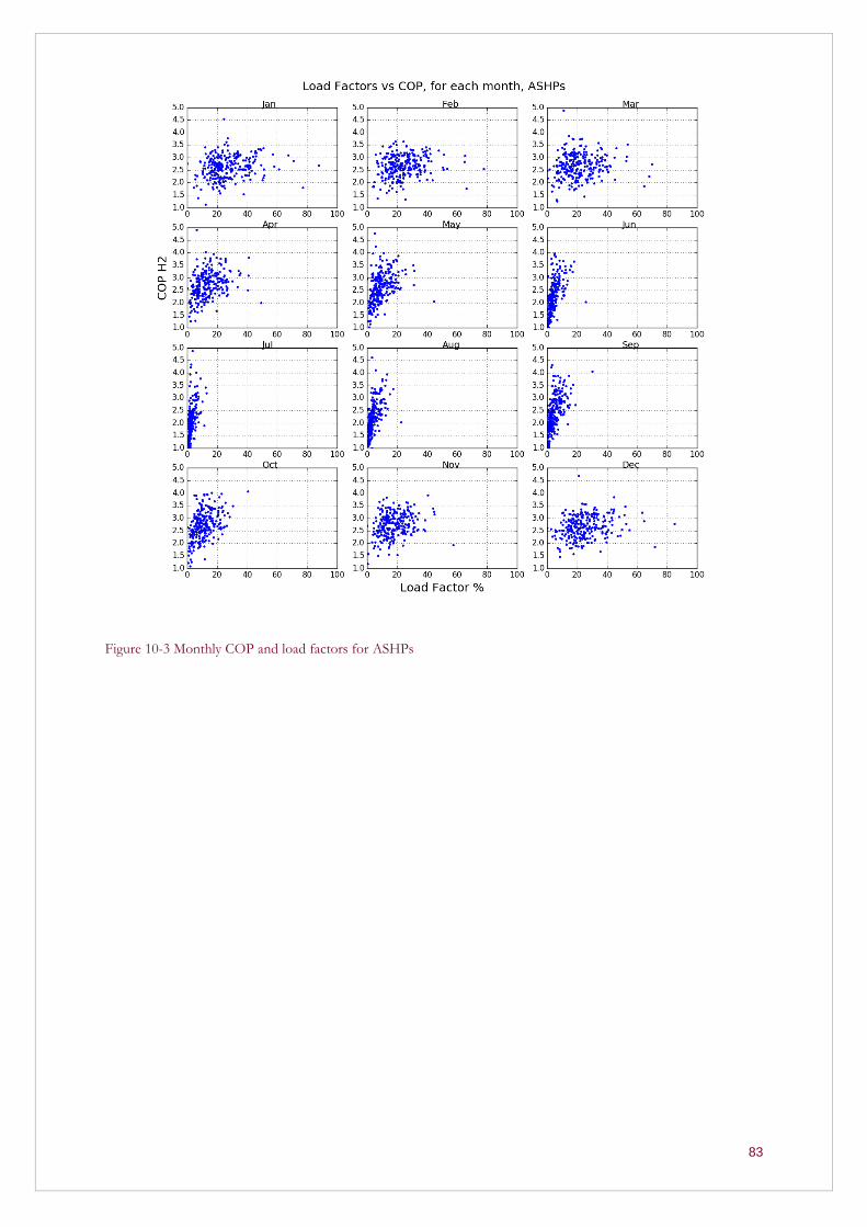
83
Figure 10-3 Monthly COP and load factors for ASHPs
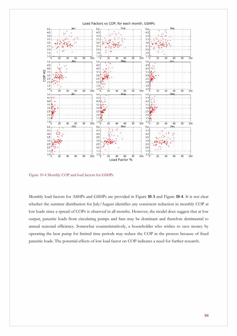
84
Figure 10-4 Monthly COP and load factors for GSHPs
Monthly load factors for ASHPs and GSHPs are provided in Figure 10-3 and Figure 10-4. It is not clear
whether the summer distribution for July/August identifies any consistent reduction in monthly COP at
low loads since a spread of COPs is observed in all months. However, the model does suggest that at low
output, parasitic loads from circulating pumps and fans may be dominant and therefore detrimental to
annual seasonal efficiency. Somewhat counterintuitively, a householder who wishes to save money by
operating the heat pump for limited time periods may reduce the COP in the process because of fixed
parasitic loads. The potential effects of low load factor on COP indicates a need for further research.

[LJJ©l ENERGY ~ ~~u~u[LJJu~
'tJjjJ 'tJjjJ
W
BS UNI~ERSITYOF SP WESTMI NSTERIIIII