report on assessment of tracks d2 - destination rail
TRANSCRIPT
DESTination RAIL – Decision Support Tool for Rail Infrastructure Managers Project Reference: 636285 H2020-MG 2014-2015 Innovations and Networks Executive Agency Project Duration: 1 May 2015–31 April 2018
Date: 21st November 2017 Dissemination level: (PU, PP, RE, CO): PU This project has received funding from the European Union’s Horizon 2020 research and innovation program under grant agreement No 636285
Report on Assessment of Tracks
D2.4
Authors
Kangle Chen (TUM), *Bernhard Lechner (TUM)
*Corresponding author: Bernhard Lechner, [email protected]
D2.4 Report on Assessment of Tracks
DESTination RAIL – Decision Support Tool for Rail Infrastructure Managers
2
DOCUMENT HISTORY
Number Date Author(s) Comments
01 30/10/2017 KC/BL
For Review
02 21/11/2017 KC/BL Review by JC (GDG)
03 13/12/2017 KC/BL Final
D2.4 Report on Assessment of Tracks
DESTination RAIL – Decision Support Tool for Rail Infrastructure Managers
3
Table of Contents
Executive Summary .............................................................................................................. 4
1 Introduction .................................................................................................................... 5
1.1 The EU-project DESTination Rail ..................................................................... 5
1.2 Tasks assigned to TU Munich .......................................................................... 5
1.3 Scope and sequence ....................................................................................... 6
2 Literature Review ........................................................................................................... 7
2.1 Track geometry and its measurement methods ............................................... 7
2.2 Track stiffness and its measurement methods ................................................. 9
2.3 Ground penetrating radar and track substructure condition ............................ 10
2.4 Conclusion of track quality monitoring methods ............................................. 12
2.5 Vehicle-Track-Interaction ............................................................................... 12
2.6 Literature review about approaches to synchronize train-borne data to track
location 13
3 Field Measurement and Data Processing .................................................................... 15
3.1 Design of field measurement ......................................................................... 15
3.2 Long section measurement and data processing ........................................... 16
3.3 Spot measurement and data processing ........................................................ 23
3.4 Conclusion ..................................................................................................... 31
4 Multi-body Simulation ................................................................................................... 32
4.1 Determination of rail seat stiffness from loaded and unloaded longitudinal level
33
4.2 Evaluation of the influence of track stiffness quality ....................................... 34
4.3 Comparison of the influence of track stiffness quality and track geometry
quality 35
4.4 Conclusion ..................................................................................................... 36
5 Conclusion and Outlook ............................................................................................... 37
6 Reference .................................................................................................................... 38
Appendix A ......................................................................................................................... 40
D2.4 Report on Assessment of Tracks
DESTination RAIL – Decision Support Tool for Rail Infrastructure Managers
4
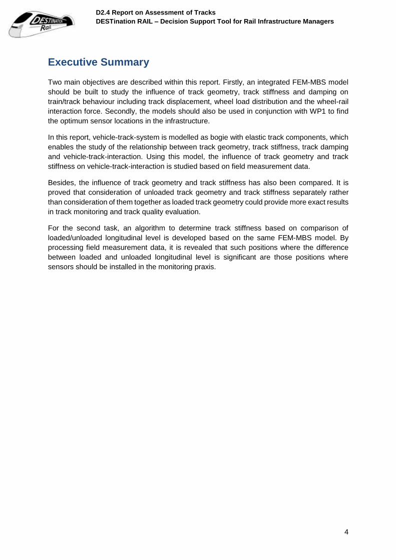
Executive Summary
Two main objectives are described within this report. Firstly, an integrated FEM-MBS model
should be built to study the influence of track geometry, track stiffness and damping on
train/track behaviour including track displacement, wheel load distribution and the wheel-rail
interaction force. Secondly, the models should also be used in conjunction with WP1 to find
the optimum sensor locations in the infrastructure.
In this report, vehicle-track-system is modelled as bogie with elastic track components, which
enables the study of the relationship between track geometry, track stiffness, track damping
and vehicle-track-interaction. Using this model, the influence of track geometry and track
stiffness on vehicle-track-interaction is studied based on field measurement data.
Besides, the influence of track geometry and track stiffness has also been compared. It is
proved that consideration of unloaded track geometry and track stiffness separately rather
than consideration of them together as loaded track geometry could provide more exact results
in track monitoring and track quality evaluation.
For the second task, an algorithm to determine track stiffness based on comparison of
loaded/unloaded longitudinal level is developed based on the same FEM-MBS model. By
processing field measurement data, it is revealed that such positions where the difference
between loaded and unloaded longitudinal level is significant are those positions where
sensors should be installed in the monitoring praxis.

D2.4 Report on Assessment of Tracks
DESTination RAIL – Decision Support Tool for Rail Infrastructure Managers
5
1 Introduction
1.1 The EU-project DESTination Rail
DESTination Rail - Decision Support Tool for Rail Infrastructure Managers is an international
scientific research project funding from European Union's Horizon 2020 research. The aim of
DESTination Rail is to provide solutions for a number of problems faced by EU infrastructure
managers. Novel techniques for identifying, analysing and remediating critical rail infrastruc-
ture has been developed. These solutions have been implemented using a decision support
tool, which allows rail infrastructure managers to make rational investment choices based on
reliable data. At present, Infrastructure Managers make safety critical investment decisions
based on poor data and an overreliance on visual assessment. Consequently, their estimates
of risk are therefore highly questionable and large-scale failures are happening with
increasingly regularity. As the European rail infrastructure network ages, investment becomes
more challenging. As a result, reliability and safety are reduced, negative user perception is
generated and the policy move to increase the use of rail transport is unsuccessful. The
objective of this project (safer, reliable and efficient rail infrastructure) is to achieve through a
holistic management tool based on the FACT (Find, Analyse, Classify, and Treat) principle.
Find – Improved techniques for the assessment of existing assets are developed.
Analyse – Advanced probabilistic models fed by performance statistics and using databases
controlled by an information management system are used to determine the level of safety of
individual assets.
Classify – The performance models allow a step-change in risk assessment, moving from the
current subjective (qualitative) basis to become fundamentally based on quantifiable data. A
decision support tool takes risk ratings and assesses the impact on the traffic flow and whole
life cycle costs of the network.
Treat – Novel and innovative maintenance and construction techniques for treating rail infra-
structure including tracks, earthworks and structures are developed and assessed by whole
life cycle assessment and impact on the traffic flow.
1.2 Tasks assigned to TU Munich
A major maintenance issue for railway infrastructure is the track itself. For this issue the
Institute of Road, Railway and Airfield Construction of Technical University of Munich (TUM)
is included in this project as participant in Task 1.3 Monitoring of Switches, Crossings and
Tracks in Work package 1 (WP 1) FIND and as group leader in Task 2.5 Assessment of Tracks
in Work Package 2 (WP 2) ANALYSE.
In WP 1 TUM has together with other colleges selected suitable data acquisition components
and integrated these into the chosen architecture. The measurement results serve for the
simulation work in WP 2.
To maximize efficiency of the modelling tools applied by TUM in WP 2 accurate referencing of
train borne data to the respective rail seats along the track (microscopic train-track-

D2.4 Report on Assessment of Tracks
DESTination RAIL – Decision Support Tool for Rail Infrastructure Managers
6
substructure modelling) is needed. However, this data is typically not provided by the
measurement trains, e.g. using measurement train data for evaluation of track quality
degradation requires synchronization of the data according to track location first.
Two different approaches have been studied by TUM:
- Methods to improve track recording train data analysis of actual measurement procedures
to achieve highest accuracy concerning accurate rail seat referencing and to gain this data as
input for modelling work or for model calibration.
- Possibilities to improve data sampling of measurement trains with regard to accurate rail seat
referencing of such vehicle borne data (e.g. using the RFID technique).
In WP 2 a systematic evaluation and decision of measures for track performance improvement
has been performed based on deep understanding of the train-track as well as track-
substructure interaction by field data and numerical simulations. The most important factors
determining the capacity of tracks to handle excitation loading is track stiffness and damping
factors. There is also a connective effect between the track performance in terms of stiffness
as well as track quality in terms of actual geometrical situation (rail alignment). An integrated
FEM-MBS model has been built for analysing the train-runs along track sections including real
track geometry and track stiffness. The output of the model includes both results related to
train and track behaviour, like the displacement of the track, the wheel load distribution and
the wheel-rail interaction force. The model is used to study the design requirements for new
track infrastructures for mixed train traffic. The models have also been used in conjunction
with WP1 to find the optimum sensor locations in the infrastructure.
1.3 Scope and sequence
The assigned tasks are interpreted as the following two sub-tasks:
to study the feasibility of different approaches to synchronize train-borne data to track
location
to establish numeric model to evaluate track quality with respect to track stiffness and
track geometry
In chapter 3, the up-to-date train borne and track borne track monitoring methods as well as
technique to synchronize them have been reviewed. A combination of suitable methods with
proper method to synchronize their data together has been selected for data acquisition to
evaluated track quality. In the chapter, the possibility to synchronize train-borne data to track
location has also been studied.
Based on the conclusions in chapter 3, field measurement has been performed. The process
of the measurement and the acquired data are showed in chapter 4.
In chapter 5 the measurement data has been processed with the help of Finite-Element-
Method (FEM) and Multi-Body-Simulation (MBS) to reveal the underlying track characteristic.
In chapter 6 conclusion and further outlook is summarized.
D2.4 Report on Assessment of Tracks
DESTination RAIL – Decision Support Tool for Rail Infrastructure Managers
7
2 Literature Review
Track quality is influenced from trackside by track geometry and track stiffness. As a first step,
reviewing of existing measurement methods as well as the related theoretical research have
been performed to find the gap in track quality monitoring activities to be filled.
2.1 Track geometry and its measurement methods
2.1.1 Track geometry and its characteristic
Track geometry is essentially the variation of lateral and vertical track position in relation to
the longitudinal position (Iwnicki, 2006). This is generally referred to as design geometry (track
layout, designed shape or alignment) and deviations from it (irregularities, roughness and track
geometry quality) (Haigermoser et al., 2015).
The measurement of track geometry comes from the first day of track. After a long time of
disordered standards of track geometry measurement all over Europa, different IMs in Europa
are now measuring and evaluating the track geometry under the unified standards EN 13848.
The item of the to be measured track geometry includes rail gauge, longitudinal level, cross
level, alignment and twist. The exact definition of these parameters could be found in EN
13848-1.
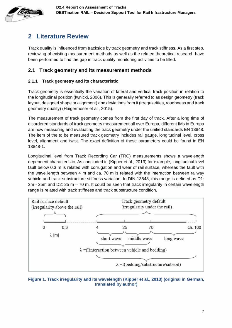
Longitudinal level from Track Recording Car (TRC) measurements shows a wavelength
dependent characteristic. As concluded in (Kipper et al., 2013) for example, longitudinal level
fault below 0.3 m is related with corrugation and wear of rail surface, whereas the fault with
the wave length between 4 m and ca. 70 m is related with the interaction between railway
vehicle and track substructure stiffness variation. In DIN 13848, this range is defined as D1:
3m - 25m and D2: 25 m – 70 m. It could be seen that track irregularity in certain wavelength
range is related with track stiffness and track substructure condition.
Figure 1. Track irregularity and its wavelength (Kipper et al., 2013) (original in German, translated by author)
D2.4 Report on Assessment of Tracks
DESTination RAIL – Decision Support Tool for Rail Infrastructure Managers
8
Commonly track geometry measurement system can be divided into moving-chord-method
measurement system and inertial measurement system according to its measurement
principal. To illustrate the working principles, two track geometry measurement equipment are
quoted here as example: RAILab from DB utilizing inertial measurement system measuring
loaded track geometry, and track measurement trolley MessRegCLS from the company Vogel
& Plötscher based on moving-chord-method measuring unloaded track geometry.
2.1.2 Inertial measurement system
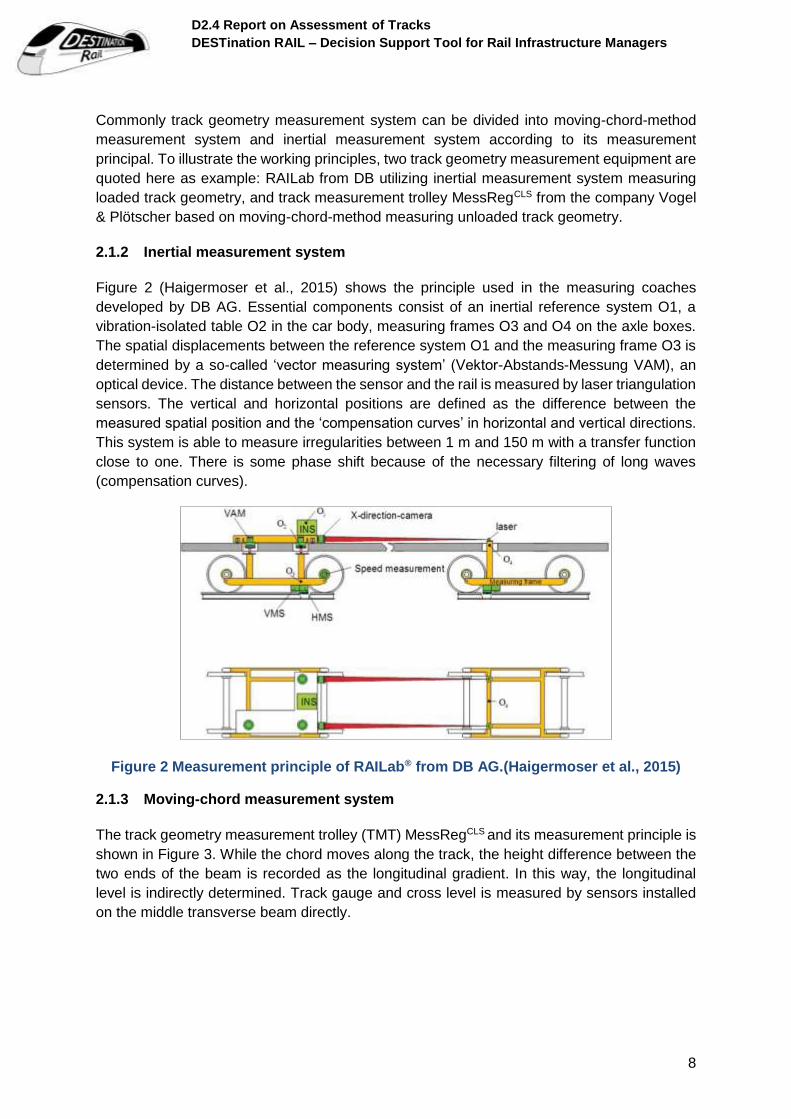
Figure 2 (Haigermoser et al., 2015) shows the principle used in the measuring coaches
developed by DB AG. Essential components consist of an inertial reference system O1, a
vibration-isolated table O2 in the car body, measuring frames O3 and O4 on the axle boxes.
The spatial displacements between the reference system O1 and the measuring frame O3 is
determined by a so-called ‘vector measuring system’ (Vektor-Abstands-Messung VAM), an
optical device. The distance between the sensor and the rail is measured by laser triangulation
sensors. The vertical and horizontal positions are defined as the difference between the
measured spatial position and the ‘compensation curves’ in horizontal and vertical directions.
This system is able to measure irregularities between 1 m and 150 m with a transfer function
close to one. There is some phase shift because of the necessary filtering of long waves
(compensation curves).
Figure 2 Measurement principle of RAILab® from DB AG.(Haigermoser et al., 2015)
2.1.3 Moving-chord measurement system
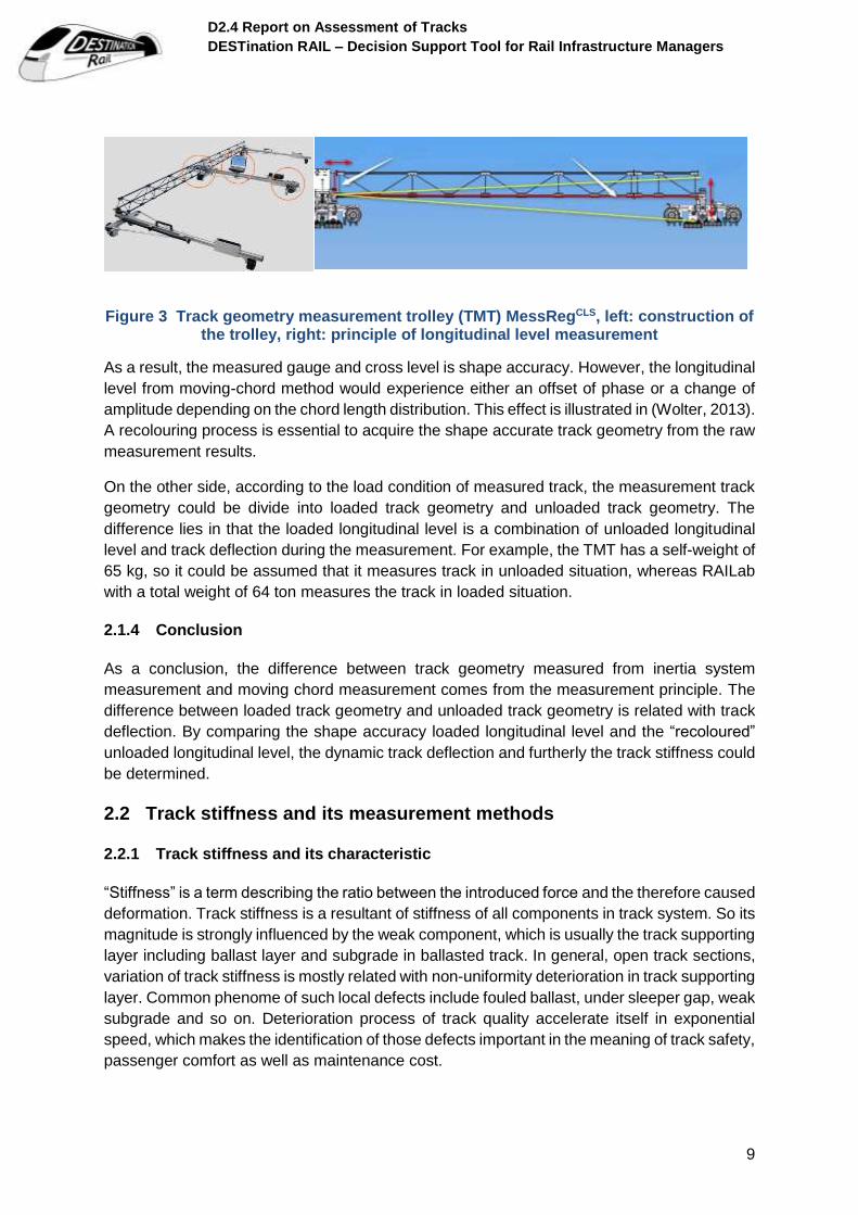
The track geometry measurement trolley (TMT) MessRegCLS and its measurement principle is
shown in Figure 3. While the chord moves along the track, the height difference between the
two ends of the beam is recorded as the longitudinal gradient. In this way, the longitudinal
level is indirectly determined. Track gauge and cross level is measured by sensors installed
on the middle transverse beam directly.
D2.4 Report on Assessment of Tracks
DESTination RAIL – Decision Support Tool for Rail Infrastructure Managers
9
Figure 3 Track geometry measurement trolley (TMT) MessRegCLS, left: construction of the trolley, right: principle of longitudinal level measurement
As a result, the measured gauge and cross level is shape accuracy. However, the longitudinal
level from moving-chord method would experience either an offset of phase or a change of
amplitude depending on the chord length distribution. This effect is illustrated in (Wolter, 2013).
A recolouring process is essential to acquire the shape accurate track geometry from the raw
measurement results.
On the other side, according to the load condition of measured track, the measurement track
geometry could be divide into loaded track geometry and unloaded track geometry. The
difference lies in that the loaded longitudinal level is a combination of unloaded longitudinal
level and track deflection during the measurement. For example, the TMT has a self-weight of
65 kg, so it could be assumed that it measures track in unloaded situation, whereas RAILab
with a total weight of 64 ton measures the track in loaded situation.
2.1.4 Conclusion
As a conclusion, the difference between track geometry measured from inertia system
measurement and moving chord measurement comes from the measurement principle. The
difference between loaded track geometry and unloaded track geometry is related with track
deflection. By comparing the shape accuracy loaded longitudinal level and the “recoloured”
unloaded longitudinal level, the dynamic track deflection and furtherly the track stiffness could
be determined.
2.2 Track stiffness and its measurement methods
2.2.1 Track stiffness and its characteristic
“Stiffness” is a term describing the ratio between the introduced force and the therefore caused
deformation. Track stiffness is a resultant of stiffness of all components in track system. So its
magnitude is strongly influenced by the weak component, which is usually the track supporting
layer including ballast layer and subgrade in ballasted track. In general, open track sections,
variation of track stiffness is mostly related with non-uniformity deterioration in track supporting
layer. Common phenome of such local defects include fouled ballast, under sleeper gap, weak
subgrade and so on. Deterioration process of track quality accelerate itself in exponential
speed, which makes the identification of those defects important in the meaning of track safety,
passenger comfort as well as maintenance cost.
D2.4 Report on Assessment of Tracks
DESTination RAIL – Decision Support Tool for Rail Infrastructure Managers
10
2.2.2 Track stiffness measurement methods
In this context, numerous measurement methods to determine track stiffness have been
developed in the past years. As indicated by its definition, to determine track stiffness,
excitation and the caused track answer should be collected.
According to type of excitation, the measurement methods could be divided into dynamic
measurement methods, impulse measurement methods and (quasi-)static methods. Track
stiffness shows strongly non-linearity and frequency-depended characteristic. Therefore, the
measured stiffness under external load of different amplitude and frequency could vary
strongly.
According to where the sensors are installed, those measurement methods could be divided
into track-borne measurement methods and train-borne measurement methods. The most
commonly used sensors include inductive transducer, strain gauge, velocimeter and
accelerometer. For track-borne methods, the deflection, velocity of deflection or acceleration
of track is collected under train-runs or under other manual introduced load. An example is
shown in (Liu, 2015). For train-borne methods, the vehicle-track-interaction is represented by
vehicle answer like axle acceleration or by measuring the track answer from vehicle. An
example is shown in (Berggren, 2009). Comparing the two methods, train-borne measurement
methods enables the possibility to collect data along long section efficiently, but it requires
specially equipped vehicle, whereas track-borne measurement methods provides access to
investigation of a short section of track conveniently, but it is not suitable for long section
measurement.
Summary of those measurement methods are well concluded in (Berg et al., Wang et al.,
2016), which would not be repeated here. It could be concluded that on one side, track
stiffness measurement is important; on the other hand, a direct method of track stiffness
measurement, which is both efficient and convenient, is not yet available.
2.3 Ground penetrating radar and track substructure condition
Nearly 20 years ago, Ground Penetration Radar (GPR) began to find its application in the area
of railway engineering in ballast layer and underground monitoring, and now it shows great
progress.
GPR is a geophysical imaging method based on measuring reflected electromagnetic (EM)
waves transmitted in the form of radar pulses in the microwave band of the radio spectrum
(UHF/VHF frequencies). A transmitting di-pole antenna radiates EM pulses into the ground
and a receiving di-pole antenna measures variations in the reflected signal in a time domain
profile. Reflections occur as the signal moves through heterogeneous material interfaces
between two media of differing dielectric properties. (De Bold et al., 2015)
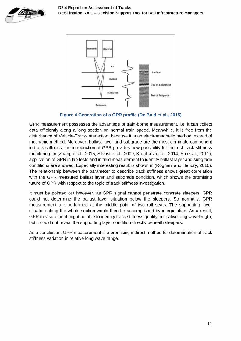
These interface reflections give responses from which the underground structural profile can
be inferred. This can be seen in Figure 4, where a diagram of a railway profile (left hand side
of the diagram) is matched against a typical radar line scan response profile (middle), and the
combination of several scans produce an underground radar profile (right). Due to its layered
nature, GPR is ideally suited for railway applications, with the possibility of data being collected
at high speeds (Clark et al., 2004).
D2.4 Report on Assessment of Tracks
DESTination RAIL – Decision Support Tool for Rail Infrastructure Managers
11
Figure 4 Generation of a GPR profile (De Bold et al., 2015)
GPR measurement possesses the advantage of train-borne measurement, i.e. it can collect
data efficiently along a long section on normal train speed. Meanwhile, it is free from the
disturbance of Vehicle-Track-Interaction, because it is an electromagnetic method instead of
mechanic method. Moreover, ballast layer and subgrade are the most dominate component
in track stiffness, the introduction of GPR provides new possibility for indirect track stiffness
monitoring. In (Zhang et al., 2015, Silvast et al., 2009, Kruglikov et al., 2014, Su et al., 2011),
application of GPR in lab tests and in field measurement to identify ballast layer and subgrade
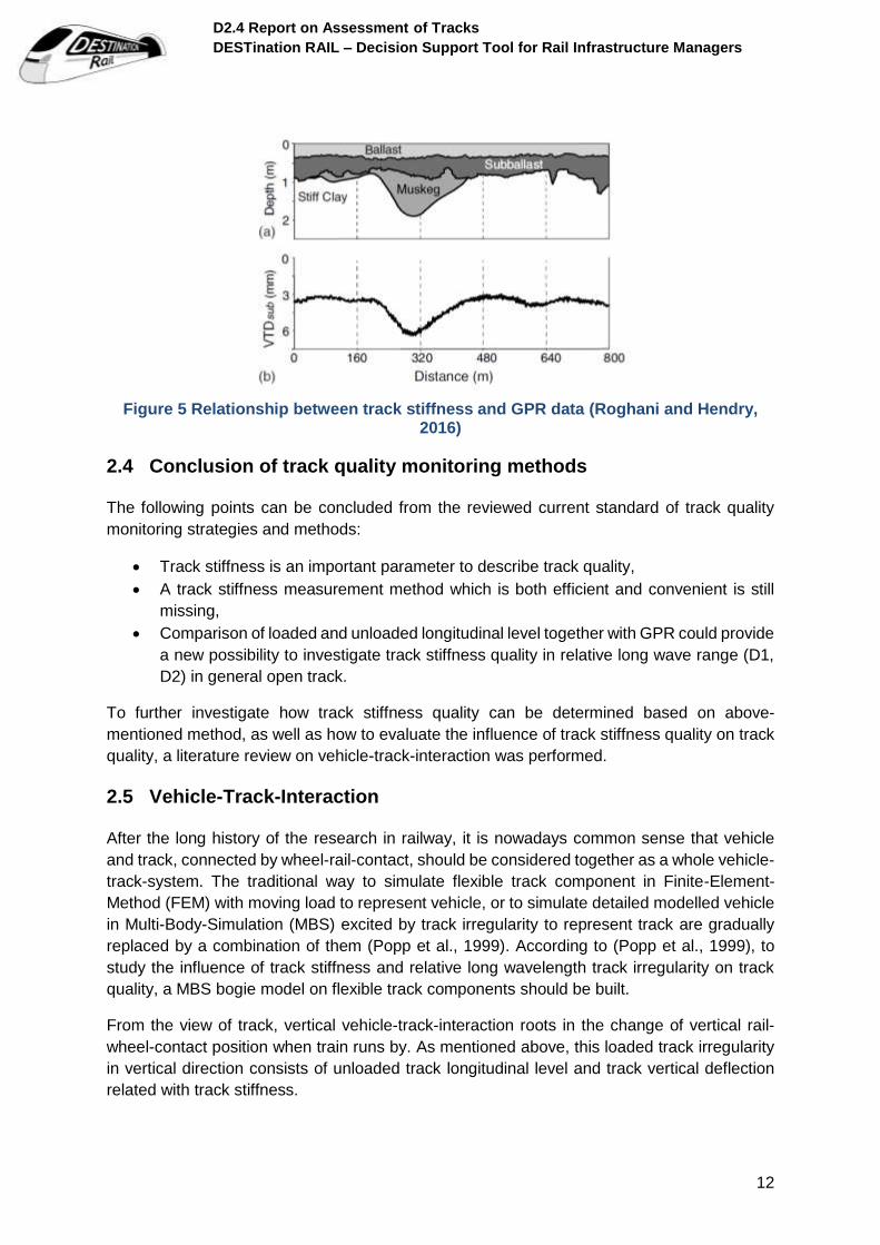
conditions are showed. Especially interesting result is shown in (Roghani and Hendry, 2016).
The relationship between the parameter to describe track stiffness shows great correlation
with the GPR measured ballast layer and subgrade condition, which shows the promising
future of GPR with respect to the topic of track stiffness investigation.
It must be pointed out however, as GPR signal cannot penetrate concrete sleepers, GPR
could not determine the ballast layer situation below the sleepers. So normally, GPR
measurement are performed at the middle point of two rail seats. The supporting layer
situation along the whole section would then be accomplished by interpolation. As a result,
GPR measurement might be able to identify track stiffness quality in relative long wavelength,
but it could not reveal the supporting layer condition directly beneath sleepers.
As a conclusion, GPR measurement is a promising indirect method for determination of track
stiffness variation in relative long wave range.
D2.4 Report on Assessment of Tracks
DESTination RAIL – Decision Support Tool for Rail Infrastructure Managers
12
Figure 5 Relationship between track stiffness and GPR data (Roghani and Hendry, 2016)
2.4 Conclusion of track quality monitoring methods
The following points can be concluded from the reviewed current standard of track quality
monitoring strategies and methods:
Track stiffness is an important parameter to describe track quality,
A track stiffness measurement method which is both efficient and convenient is still
missing,
Comparison of loaded and unloaded longitudinal level together with GPR could provide
a new possibility to investigate track stiffness quality in relative long wave range (D1,
D2) in general open track.
To further investigate how track stiffness quality can be determined based on above-
mentioned method, as well as how to evaluate the influence of track stiffness quality on track
quality, a literature review on vehicle-track-interaction was performed.
2.5 Vehicle-Track-Interaction
After the long history of the research in railway, it is nowadays common sense that vehicle
and track, connected by wheel-rail-contact, should be considered together as a whole vehicle-
track-system. The traditional way to simulate flexible track component in Finite-Element-
Method (FEM) with moving load to represent vehicle, or to simulate detailed modelled vehicle
in Multi-Body-Simulation (MBS) excited by track irregularity to represent track are gradually
replaced by a combination of them (Popp et al., 1999). According to (Popp et al., 1999), to
study the influence of track stiffness and relative long wavelength track irregularity on track
quality, a MBS bogie model on flexible track components should be built.
From the view of track, vertical vehicle-track-interaction roots in the change of vertical rail-
wheel-contact position when train runs by. As mentioned above, this loaded track irregularity
in vertical direction consists of unloaded track longitudinal level and track vertical deflection
related with track stiffness.
D2.4 Report on Assessment of Tracks
DESTination RAIL – Decision Support Tool for Rail Infrastructure Managers
13
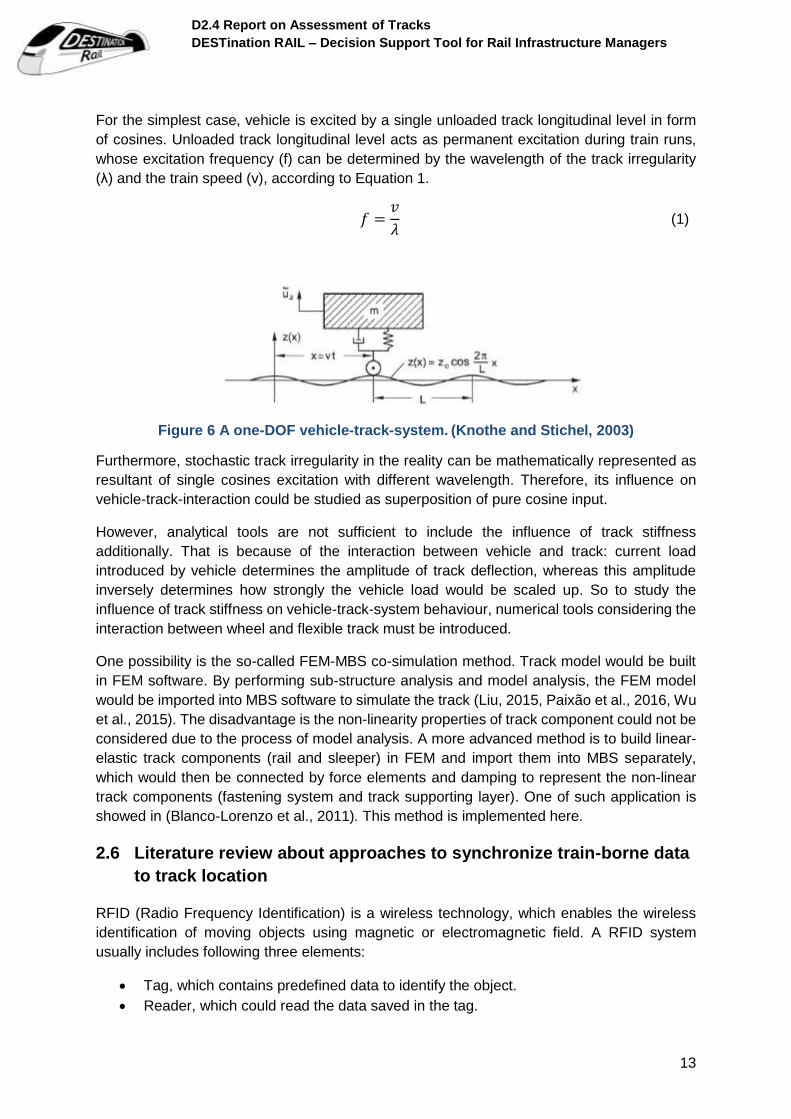
For the simplest case, vehicle is excited by a single unloaded track longitudinal level in form
of cosines. Unloaded track longitudinal level acts as permanent excitation during train runs,
whose excitation frequency (f) can be determined by the wavelength of the track irregularity
(λ) and the train speed (v), according to Equation 1.
𝑓 =𝑣
𝜆 (1)
Figure 6 A one-DOF vehicle-track-system. (Knothe and Stichel, 2003)
Furthermore, stochastic track irregularity in the reality can be mathematically represented as
resultant of single cosines excitation with different wavelength. Therefore, its influence on
vehicle-track-interaction could be studied as superposition of pure cosine input.
However, analytical tools are not sufficient to include the influence of track stiffness
additionally. That is because of the interaction between vehicle and track: current load
introduced by vehicle determines the amplitude of track deflection, whereas this amplitude
inversely determines how strongly the vehicle load would be scaled up. So to study the
influence of track stiffness on vehicle-track-system behaviour, numerical tools considering the
interaction between wheel and flexible track must be introduced.
One possibility is the so-called FEM-MBS co-simulation method. Track model would be built
in FEM software. By performing sub-structure analysis and model analysis, the FEM model
would be imported into MBS software to simulate the track (Liu, 2015, Paixão et al., 2016, Wu
et al., 2015). The disadvantage is the non-linearity properties of track component could not be
considered due to the process of model analysis. A more advanced method is to build linear-
elastic track components (rail and sleeper) in FEM and import them into MBS separately,
which would then be connected by force elements and damping to represent the non-linear
track components (fastening system and track supporting layer). One of such application is
showed in (Blanco-Lorenzo et al., 2011). This method is implemented here.
2.6 Literature review about approaches to synchronize train-borne data
to track location
RFID (Radio Frequency Identification) is a wireless technology, which enables the wireless
identification of moving objects using magnetic or electromagnetic field. A RFID system
usually includes following three elements:
Tag, which contains predefined data to identify the object.
Reader, which could read the data saved in the tag.

D2.4 Report on Assessment of Tracks
DESTination RAIL – Decision Support Tool for Rail Infrastructure Managers
14
A computer system, which could resolve and process the data read by the reader.
Each RFID tag is made up of two components: integrated circuit to store information on the
chip and antenna for transmitting that information to a remote place. There are two types of
tags: active tags that relate to batteries for energy, and passive tags that are getting energy
transmitted from readers. These tags transmit the data in the form of either low, high, ultra-
high or microwave frequency based on the amount of data to be transmitted.
RFID Readers are the coil of wire known as antenna used to transmit the distance signal. The
antenna is used for various purpose such as to power tags by sending query signals, encoding
data on chips and decoding the data from the chip. The frequency on which the RFID operate
is around 30 KHz to 500 KHz, 850 MHz to 950 MHz and 2.4GHz to 2.5GHz. With the time,
there is a lot of advancement occur in reader such as development of anti-collision software
that prevent the reader to get the data from more than one tag at a time and to prevent the
unauthorized access to transmitted data.
RFID systems are widely used in many industry sectors for the purpose of detection and
identification, so it is mentioned in the proposal, whether it is possible to implement RIFD
system in track monitoring system for synchronization of train position to track. After study of
the technical parameters of RFID systems, it is concluded that it is not applicable. The main
problem is the range of RFID system to recognize the tags lies around 0.5 m, which is not
accurate enough for exactly synchronization of train measurement data with respect to rail
seats, while the rail seat distance lies usually between 0.6 m and 0.7 m. At present, RFID
systems are suitable for such tasks like identification rather than for synchronization.

D2.4 Report on Assessment of Tracks
DESTination RAIL – Decision Support Tool for Rail Infrastructure Managers
15
3 Field Measurement and Data Processing
Based on the aim of the research and the literature review, the following measurements have
been performed:
loaded track geometry measurement
unloaded track geometry measurement
GPR measurement
The aim of this study is concluded as follows:
To evaluate the possibility of synchronizing the train borne measurement data with
track position.
To provide the data for track quality evaluation.
3.1 Design of field measurement
3.1.1 Selection of measurement section
TUM initiated meetings with Deutsche Bahn (DB) representatives in 2015 to receive support
for the DESTination RAIL project by a pilot section suitable to perform trackside
measurements for model validation and simulation. DB helped TUM to select a track section
of a railway line in the south of the city of Munich, which is an old, conventional ballasted line
with the superstructure component of Rail S 54 rail fastening system and concrete sleeper B
58 K. This section was chosen based on following consideration:
The radius of the section is larger than 2000 m, which could be considered as straight
track; The line is horizontal, train speed (Vmax = 140 km/h) is constant and traction force
is low (no station/stop close to the pilot section);
The section shows no discontinuities along the superstructure (track form) or
substructure type like transitions, bridge decks, under crossing etc., and can be
considered as a homogenous section;
Beside the general track quality level, the measurement results from DB’s track
recording car RAILab® show noticeable track geometry faults with unknown source.
In conclusion, this section is characterized as straight, homogenous section of normal track
quality with existing track geometry faults. It represents typical open track section and thus it
is an ideal starting section for the issue of track monitoring method development.
3.1.2 Selection of measurement methods
The chosen measurements methods / equip are concluded in Table 1:
D2.4 Report on Assessment of Tracks
DESTination RAIL – Decision Support Tool for Rail Infrastructure Managers
16
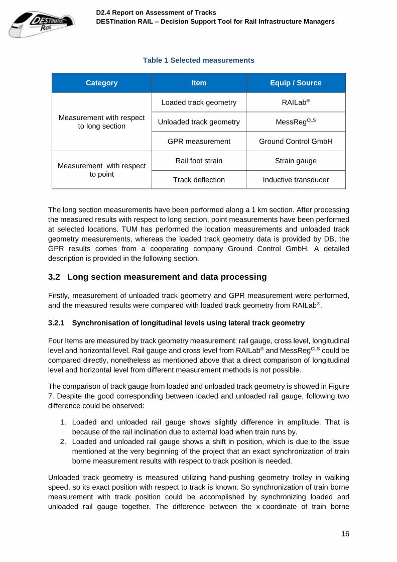
Table 1 Selected measurements
Category Item Equip / Source
Measurement with respect to long section
Loaded track geometry RAILab®
Unloaded track geometry MessRegCLS
GPR measurement Ground Control GmbH
Measurement with respect to point
Rail foot strain Strain gauge
Track deflection Inductive transducer
The long section measurements have been performed along a 1 km section. After processing
the measured results with respect to long section, point measurements have been performed
at selected locations. TUM has performed the location measurements and unloaded track
geometry measurements, whereas the loaded track geometry data is provided by DB, the
GPR results comes from a cooperating company Ground Control GmbH. A detailed
description is provided in the following section.
3.2 Long section measurement and data processing
Firstly, measurement of unloaded track geometry and GPR measurement were performed,
and the measured results were compared with loaded track geometry from RAILab®.
3.2.1 Synchronisation of longitudinal levels using lateral track geometry
Four Items are measured by track geometry measurement: rail gauge, cross level, longitudinal
level and horizontal level. Rail gauge and cross level from RAILab® and MessRegCLS could be
compared directly, nonetheless as mentioned above that a direct comparison of longitudinal
level and horizontal level from different measurement methods is not possible.
The comparison of track gauge from loaded and unloaded track geometry is showed in Figure
7. Despite the good corresponding between loaded and unloaded rail gauge, following two
difference could be observed:
1. Loaded and unloaded rail gauge shows slightly difference in amplitude. That is
because of the rail inclination due to external load when train runs by.
2. Loaded and unloaded rail gauge shows a shift in position, which is due to the issue
mentioned at the very beginning of the project that an exact synchronization of train
borne measurement results with respect to track position is needed.
Unloaded track geometry is measured utilizing hand-pushing geometry trolley in walking
speed, so its exact position with respect to track is known. So synchronization of train borne
measurement with track position could be accomplished by synchronizing loaded and
unloaded rail gauge together. The difference between the x-coordinate of train borne
D2.4 Report on Assessment of Tracks
DESTination RAIL – Decision Support Tool for Rail Infrastructure Managers
17
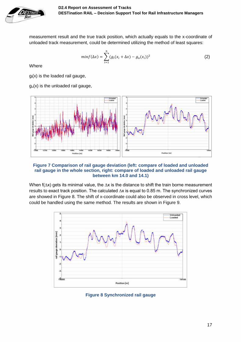
measurement result and the true track position, which actually equals to the x-coordinate of
unloaded track measurement, could be determined utilizing the method of least squares:
𝑚𝑖𝑛𝑓(∆𝑥) = ∑(𝑔𝑙(𝑥𝑖 + ∆𝑥) − 𝑔𝑢(𝑥𝑖))2
𝑛
𝑖=1
(2)
Where
gl(x) is the loaded rail gauge,
gu(x) is the unloaded rail gauge,
Figure 7 Comparison of rail gauge deviation (left: compare of loaded and unloaded rail gauge in the whole section, right: compare of loaded and unloaded rail gauge
between km 14.0 and 14.1)
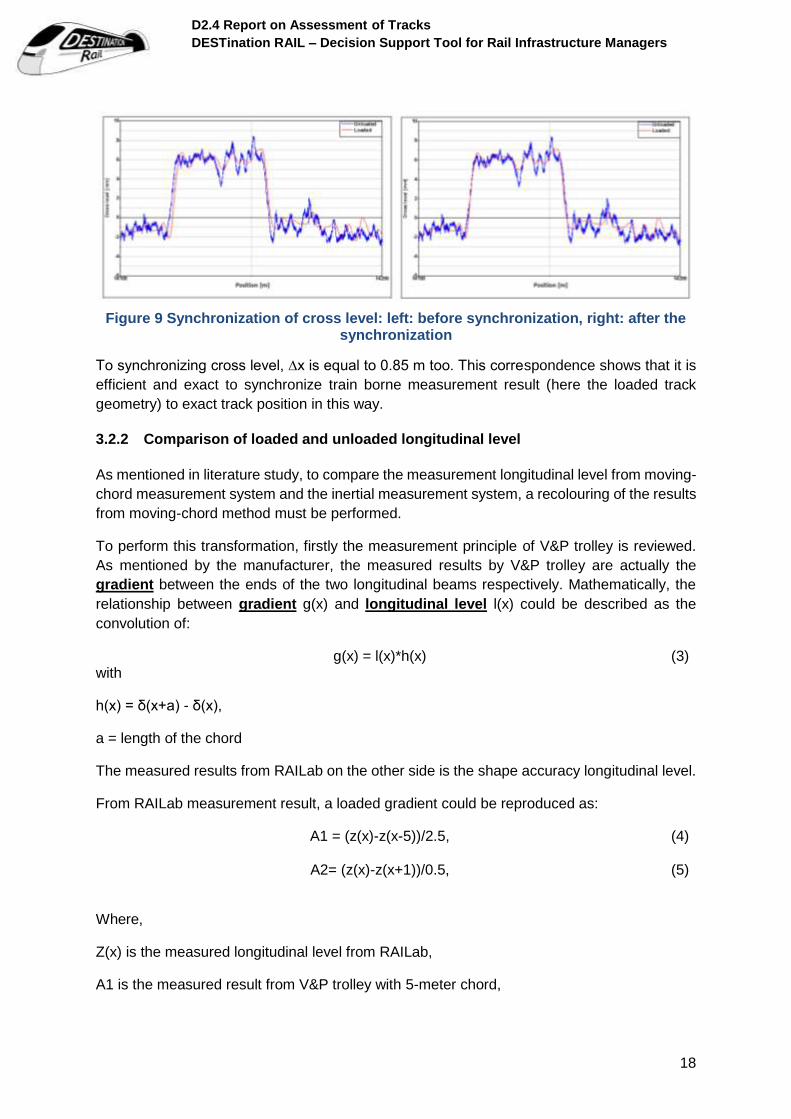
When f(∆x) gets its minimal value, the ∆x is the distance to shift the train borne measurement
results to exact track position. The calculated ∆x is equal to 0.85 m. The synchronized curves
are showed in Figure 8. The shift of x-coordinate could also be observed in cross level, which
could be handled using the same method. The results are shown in Figure 9.
Figure 8 Synchronized rail gauge
D2.4 Report on Assessment of Tracks
DESTination RAIL – Decision Support Tool for Rail Infrastructure Managers
18
Figure 9 Synchronization of cross level: left: before synchronization, right: after the synchronization
To synchronizing cross level, ∆x is equal to 0.85 m too. This correspondence shows that it is
efficient and exact to synchronize train borne measurement result (here the loaded track
geometry) to exact track position in this way.
3.2.2 Comparison of loaded and unloaded longitudinal level
As mentioned in literature study, to compare the measurement longitudinal level from moving-
chord measurement system and the inertial measurement system, a recolouring of the results
from moving-chord method must be performed.
To perform this transformation, firstly the measurement principle of V&P trolley is reviewed.
As mentioned by the manufacturer, the measured results by V&P trolley are actually the
gradient between the ends of the two longitudinal beams respectively. Mathematically, the
relationship between gradient g(x) and longitudinal level l(x) could be described as the
convolution of:
g(x) = l(x)*h(x) (3) with
h(x) = δ(x+a) - δ(x),
a = length of the chord
The measured results from RAILab on the other side is the shape accuracy longitudinal level.
From RAILab measurement result, a loaded gradient could be reproduced as:
A1 = (z(x)-z(x-5))/2.5,
(4)
A2= (z(x)-z(x+1))/0.5, (5)
Where,
Z(x) is the measured longitudinal level from RAILab,
A1 is the measured result from V&P trolley with 5-meter chord,

D2.4 Report on Assessment of Tracks
DESTination RAIL – Decision Support Tool for Rail Infrastructure Managers
19
A2 is the measured result from V&P trolley with 1-meter chord.
The sampling rate of RAILab is 0.16 m. Therefore, an exact reproduction of V&P trolley is not
possible. A1 is reproduced as 4.96 m chord, and A2 as 0.96 m chord. The results are shown
in Figure 10.
Figure 10 Comparison of measured unloaded gradient and reproduced loaded gradient, above: 5 m chord, under: 1 m chord.
Furtherly, low-pass filter has been implemented on the measured results to filter the high and
meanwhile irrelevant frequency component. The conspicuous peak at km 14020 is plotted in
Figure 13.
Page 6
Diagram
Diagram
A1
z1
A2
z2
km [m]
13.900 13.925 13.950 13.975 14.000 14.025 14.050 14.075 14.100x 10
3
A1 [
mm
]
-15
-10
-5
0
5
10
15
km [m]
13.900 13.925 13.950 13.975 14.000 14.025 14.050 14.075 14.100x 10
3
A1 [
mm
]
-6
-4
-2
0
2
4
6
8
D2.4 Report on Assessment of Tracks
DESTination RAIL – Decision Support Tool for Rail Infrastructure Managers
20
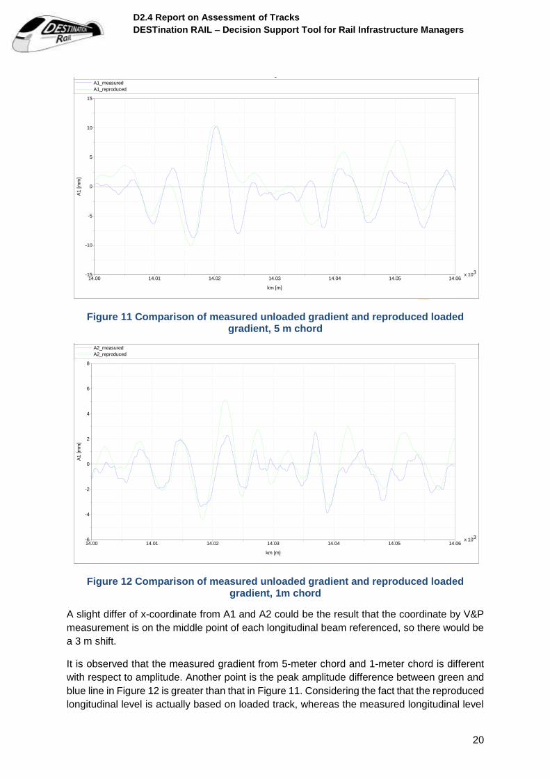
Figure 11 Comparison of measured unloaded gradient and reproduced loaded gradient, 5 m chord
Figure 12 Comparison of measured unloaded gradient and reproduced loaded gradient, 1m chord
A slight differ of x-coordinate from A1 and A2 could be the result that the coordinate by V&P
measurement is on the middle point of each longitudinal beam referenced, so there would be
a 3 m shift.
It is observed that the measured gradient from 5-meter chord and 1-meter chord is different
with respect to amplitude. Another point is the peak amplitude difference between green and
blue line in Figure 12 is greater than that in Figure 11. Considering the fact that the reproduced
longitudinal level is actually based on loaded track, whereas the measured longitudinal level
Page 2
Diagram
A1_measured
A1_reproduced
km [m]
14.00 14.01 14.02 14.03 14.04 14.05 14.06x 10
3
A1 [
mm
]
-15
-10
-5
0
5
10
15
Page 3
Diagram
A2_measured
A2_reproduced
km [m]
14.00 14.01 14.02 14.03 14.04 14.05 14.06x 10
3
A1 [
mm
]
-6
-4
-2
0
2
4
6
8
D2.4 Report on Assessment of Tracks
DESTination RAIL – Decision Support Tool for Rail Infrastructure Managers
21
is based on unloaded track, so it is inferred that this difference is related with abrupt short
wavelength deflection change, which could not be collected by 5 m chord but by 1 m chord.
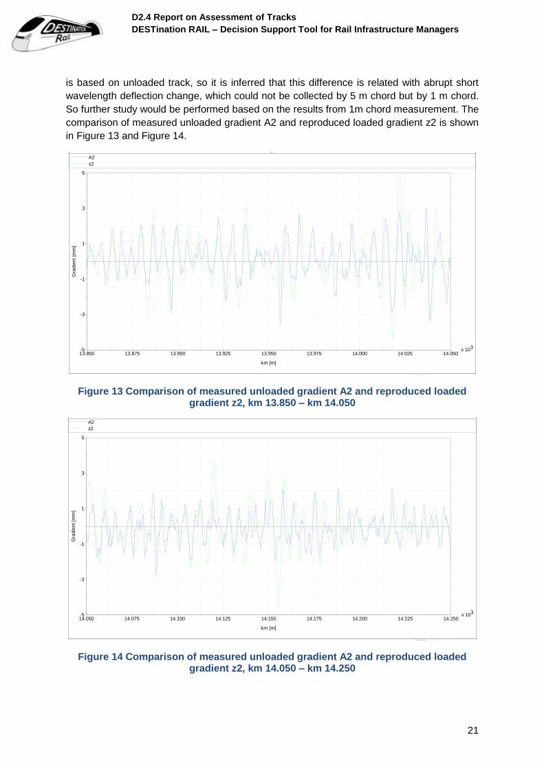
So further study would be performed based on the results from 1m chord measurement. The
comparison of measured unloaded gradient A2 and reproduced loaded gradient z2 is shown
in Figure 13 and Figure 14.
Figure 13 Comparison of measured unloaded gradient A2 and reproduced loaded gradient z2, km 13.850 – km 14.050
Figure 14 Comparison of measured unloaded gradient A2 and reproduced loaded gradient z2, km 14.050 – km 14.250
Page 8
Diagram
A2
z2
km [m]
13.850 13.875 13.900 13.925 13.950 13.975 14.000 14.025 14.050x 10
3
Gra
die
nt
[mm
]
-5
-3
-1
1
3
5
Page 8
Diagram
A2
z2
km [m]
14.050 14.075 14.100 14.125 14.150 14.175 14.200 14.225 14.250x 10
3
Gra
die
nt
[mm
]
-5
-3
-1
1
3
5
D2.4 Report on Assessment of Tracks
DESTination RAIL – Decision Support Tool for Rail Infrastructure Managers
22
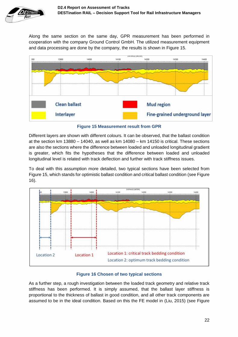
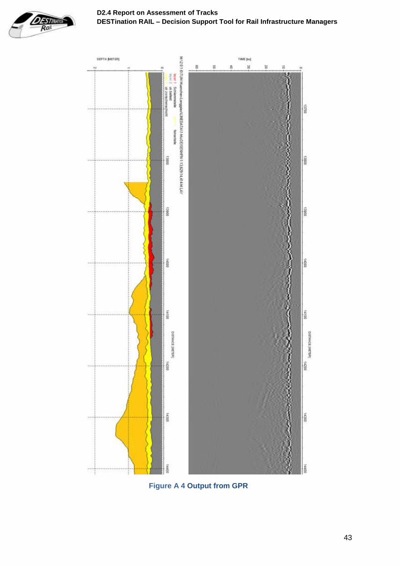
Along the same section on the same day, GPR measurement has been performed in
cooperation with the company Ground Control GmbH. The utilized measurement equipment
and data processing are done by the company, the results is shown in Figure 15.
Figure 15 Measurement result from GPR
Different layers are shown with different colours. It can be observed, that the ballast condition
at the section km 13880 – 14040, as well as km 14080 – km 14150 is critical. These sections
are also the sections where the difference between loaded and unloaded longitudinal gradient
is greater, which fits the hypotheses that the difference between loaded and unloaded
longitudinal level is related with track deflection and further with track stiffness issues.
To deal with this assumption more detailed, two typical sections have been selected from
Figure 15, which stands for optimistic ballast condition and critical ballast condition (see Figure
16).
Figure 16 Chosen of two typical sections
As a further step, a rough investigation between the loaded track geometry and relative track
stiffness has been performed. It is simply assumed, that the ballast layer stiffness is
proportional to the thickness of ballast in good condition, and all other track components are
assumed to be in the ideal condition. Based on this the FE model in (Liu, 2015) (see Figure

D2.4 Report on Assessment of Tracks
DESTination RAIL – Decision Support Tool for Rail Infrastructure Managers
23
17) has been employed here to provide the “relative deflection”, which is the track deflection
with “relative stiffness” under unit constant load. The result is shown in Figure 18.
Figure 17 FE model for "track relative deflection"
Figure 18 Comparison of Longitudinal Level and relative deflection
It can be concluded that in the section where the track stiffness level is critical, the deflection
rather than the unloaded track geometry is the main component of loaded track geometry.
3.3 Spot measurement and data processing
Based on the long section measurement result it is concluded in the above chapter that
magnitude of the difference between loaded and unloaded longitudinal level correlates to the
fouling situation of ballast layer. To prove this assumption furtherly, measurement of track
answer under train runs on two chosen typical locations have been carried out.
D2.4 Report on Assessment of Tracks
DESTination RAIL – Decision Support Tool for Rail Infrastructure Managers
24
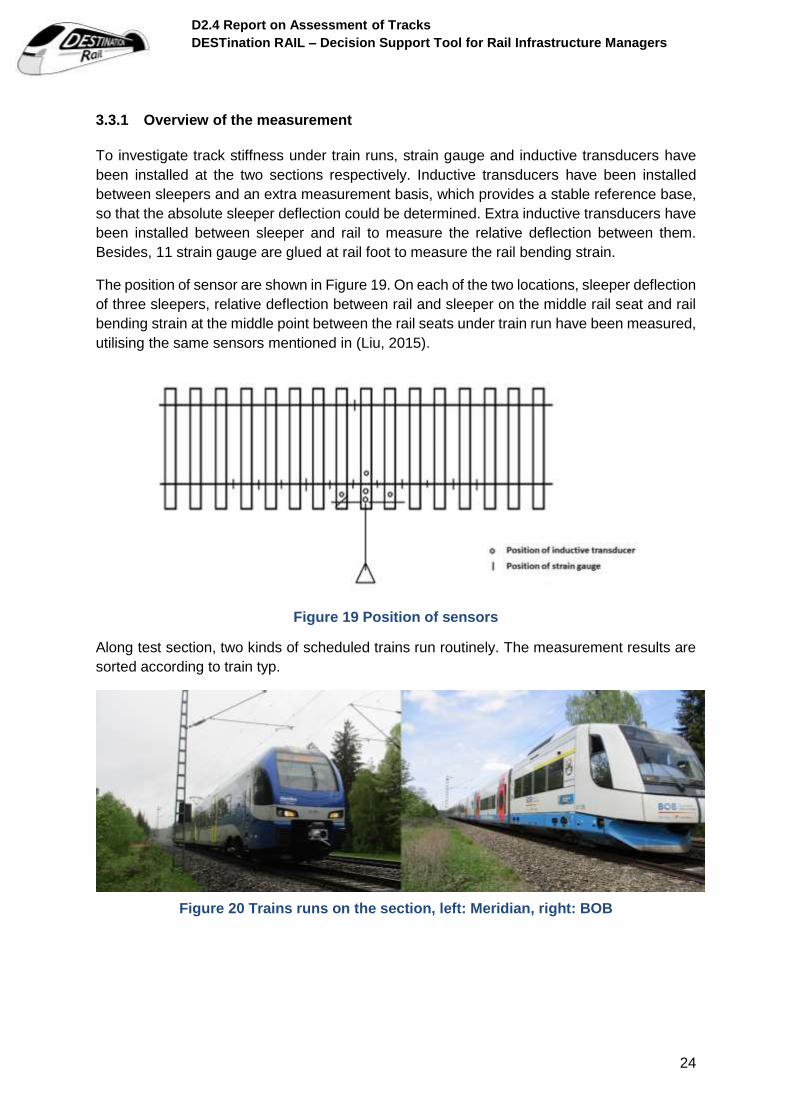
3.3.1 Overview of the measurement
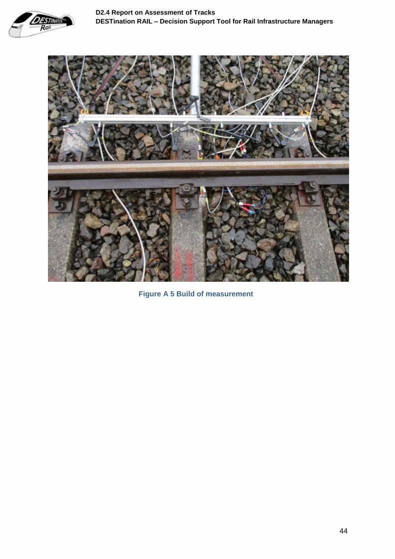
To investigate track stiffness under train runs, strain gauge and inductive transducers have
been installed at the two sections respectively. Inductive transducers have been installed
between sleepers and an extra measurement basis, which provides a stable reference base,
so that the absolute sleeper deflection could be determined. Extra inductive transducers have
been installed between sleeper and rail to measure the relative deflection between them.
Besides, 11 strain gauge are glued at rail foot to measure the rail bending strain.
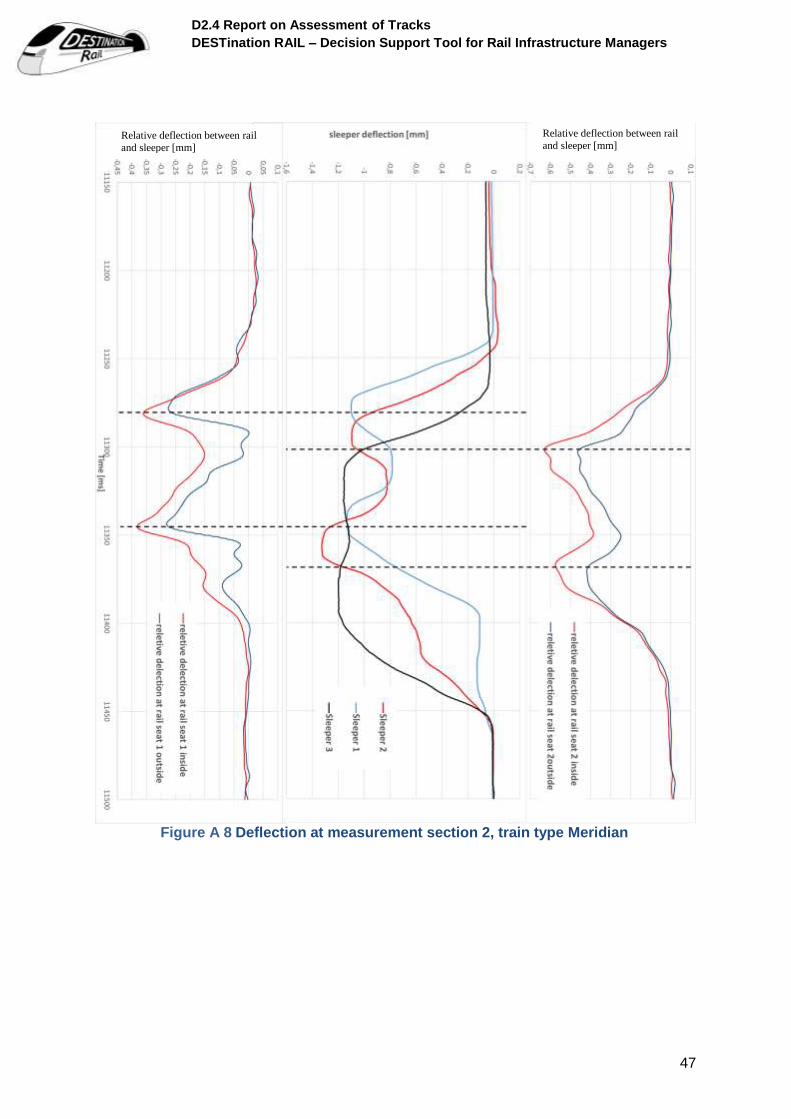
The position of sensor are shown in Figure 19. On each of the two locations, sleeper deflection
of three sleepers, relative deflection between rail and sleeper on the middle rail seat and rail
bending strain at the middle point between the rail seats under train run have been measured,
utilising the same sensors mentioned in (Liu, 2015).
Figure 19 Position of sensors
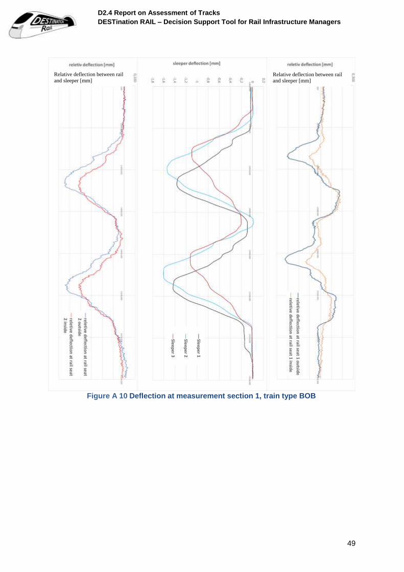
Along test section, two kinds of scheduled trains run routinely. The measurement results are
sorted according to train typ.
Figure 20 Trains runs on the section, left: Meridian, right: BOB
D2.4 Report on Assessment of Tracks
DESTination RAIL – Decision Support Tool for Rail Infrastructure Managers
25
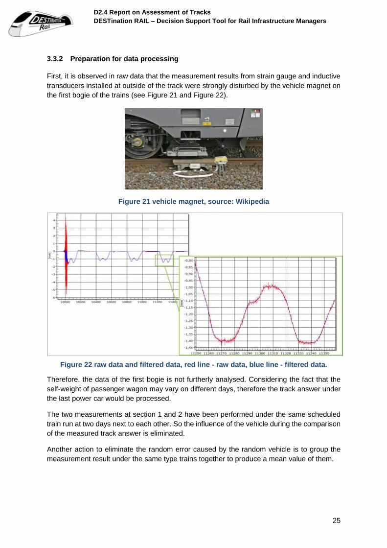
3.3.2 Preparation for data processing
First, it is observed in raw data that the measurement results from strain gauge and inductive
transducers installed at outside of the track were strongly disturbed by the vehicle magnet on
the first bogie of the trains (see Figure 21 and Figure 22).
Figure 21 vehicle magnet, source: Wikipedia
Figure 22 raw data and filtered data, red line - raw data, blue line - filtered data.
Therefore, the data of the first bogie is not furtherly analysed. Considering the fact that the
self-weight of passenger wagon may vary on different days, therefore the track answer under
the last power car would be processed.
The two measurements at section 1 and 2 have been performed under the same scheduled
train run at two days next to each other. So the influence of the vehicle during the comparison
of the measured track answer is eliminated.
Another action to eliminate the random error caused by the random vehicle is to group the
measurement result under the same type trains together to produce a mean value of them.
D2.4 Report on Assessment of Tracks
DESTination RAIL – Decision Support Tool for Rail Infrastructure Managers
26
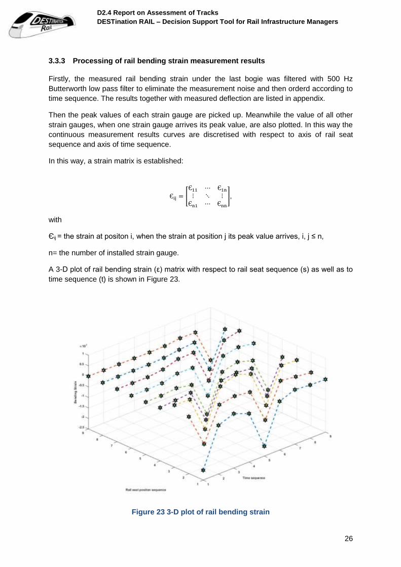
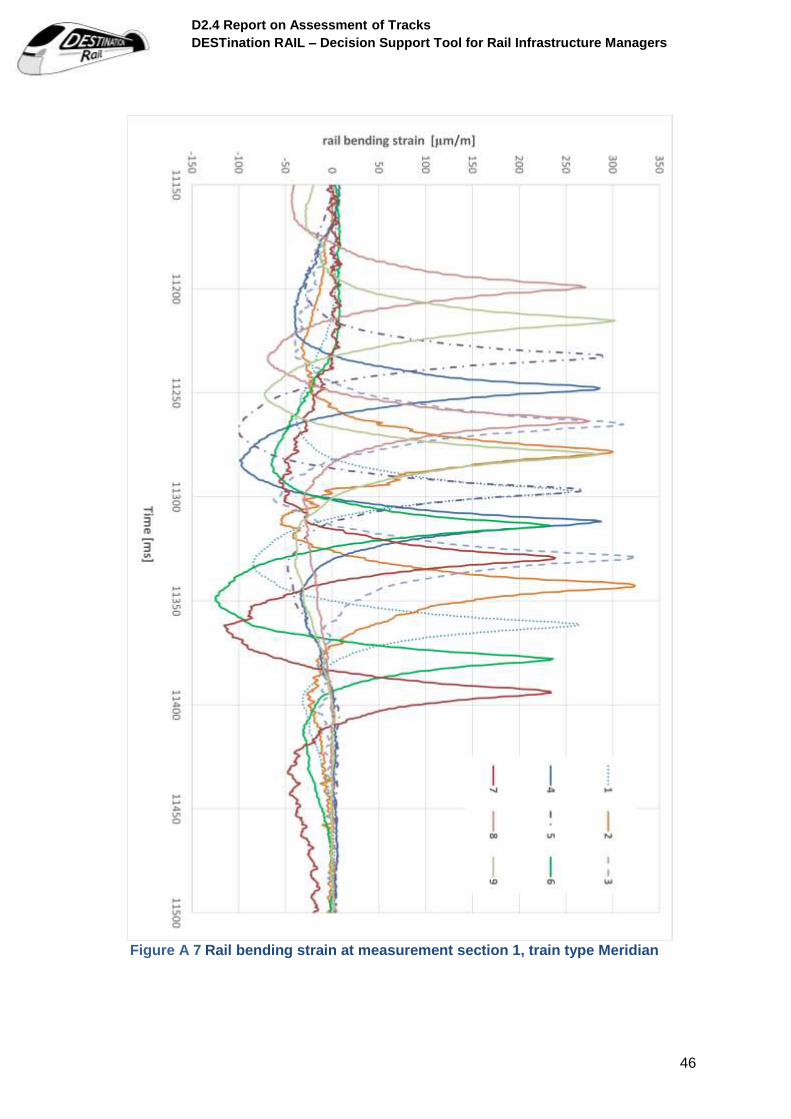
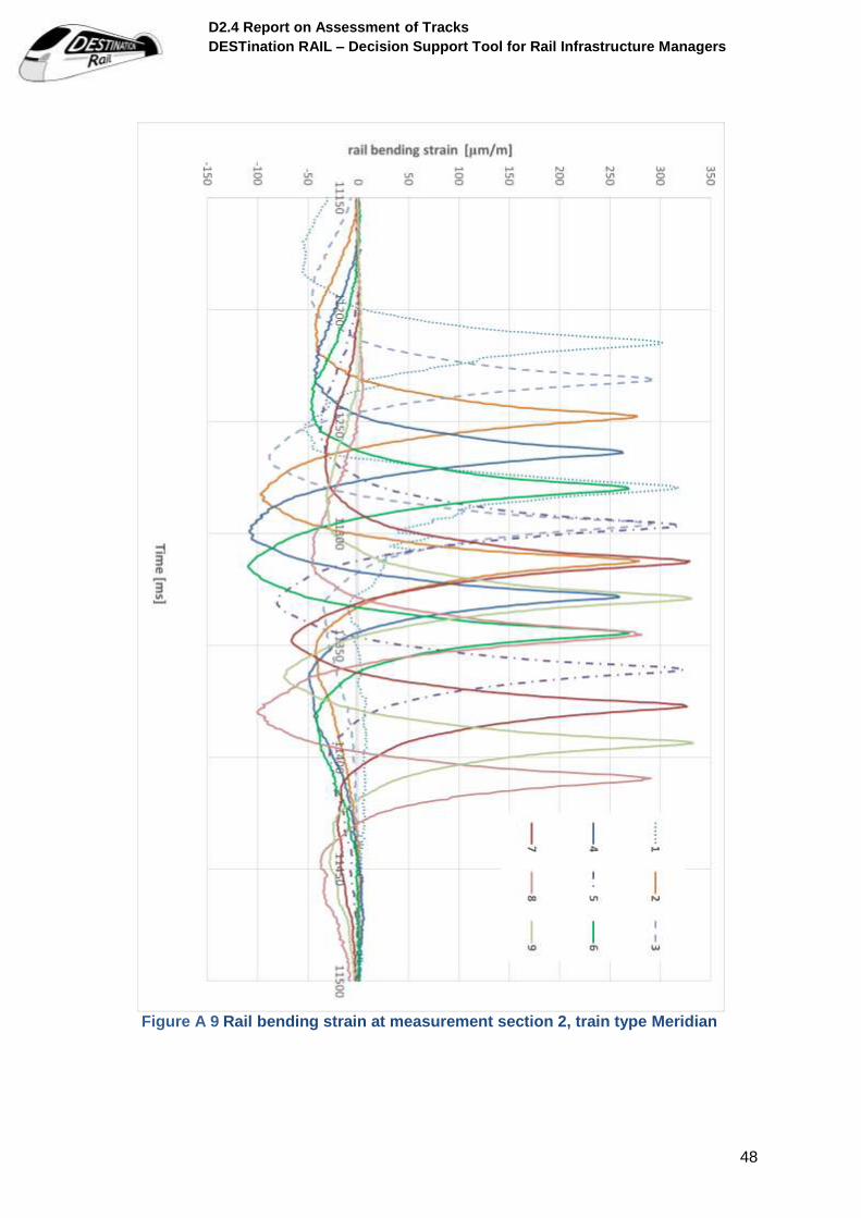
3.3.3 Processing of rail bending strain measurement results
Firstly, the measured rail bending strain under the last bogie was filtered with 500 Hz
Butterworth low pass filter to eliminate the measurement noise and then orderd according to
time sequence. The results together with measured deflection are listed in appendix.
Then the peak values of each strain gauge are picked up. Meanwhile the value of all other
strain gauges, when one strain gauge arrives its peak value, are also plotted. In this way the
continuous measurement results curves are discretised with respect to axis of rail seat
sequence and axis of time sequence.
In this way, a strain matrix is established:
Єij = [Є11 ⋯ Є1n
⋮ ⋱ ⋮Єn1 ⋯ Єnn
],
with
Єij = the strain at positon i, when the strain at position j its peak value arrives, i, j ≤ n,
n= the number of installed strain gauge.
A 3-D plot of rail bending strain (ε) matrix with respect to rail seat sequence (s) as well as to
time sequence (t) is shown in Figure 23.
Figure 23 3-D plot of rail bending strain

D2.4 Report on Assessment of Tracks
DESTination RAIL – Decision Support Tool for Rail Infrastructure Managers
27
It is self-evidence, that the measurement result of a strain gauge arrives its maximal value,
when the wheel is exactly above it. Accordingly, the train speed could be calculated based on
the time interval between the maximal value of two neighbour strain gauges and their spatial
distance, which is graphically the tangential ration of the peak value in s-t plane in Figure 23.
With the sleeper space of 0.63 m, the average speed when the train passes the two sections
is calculated as 139.4 km/h and 140.8 km/h respectively, which fits with the information from
DB that the train speed in the section should be 140 km/h. When comparing the two locations,
the influence of speed variance is thus eliminated.
When Figure 23 is cut by plane parallel to ε-t plane at s = s0, it shows the strain history of the
chosen rail seat s0 during the train runs. Such a line is shown in Figure 24.
Figure 24 Strain-time (ε-t) curve of fourth rail seat
Similarly when Figure 23 is cut by plane parallel to ε-s plane at t = t0, it shows the distribution
of rail bending strain along the measured section at this selected time point t0. An example
line in space-strain plane is shown in Figure 25.
D2.4 Report on Assessment of Tracks
DESTination RAIL – Decision Support Tool for Rail Infrastructure Managers
28
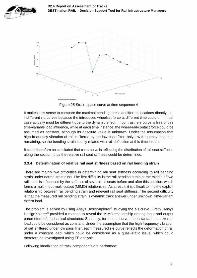
Figure 25 Strain-space curve at time sequence 4
It makes less sense to compare the maximal bending stress at different locations directly, i.e.
indifferent ε-t, curves because the introduced wheelset force at different time could or in most
case actually must be different due to the dynamic effect. In contrast, ε-s curve is free of this
time-variable load influence, while at each time instance, the wheel-rail-contact force could be
assumed as constant, although its absolute value is unknown. Under the assumption that
high-frequency vibration of rail is filtered by the low-pass-filter, only low frequency motion is
remaining, so the bending strain is only related with rail deflection at this time instant.
It could therefore be concluded that a ε-s curve is reflecting the distribution of rail seat stiffness
along the section, thus the relative rail seat stiffness could be determined.
3.3.4 Determination of relative rail seat stiffness based on rail bending strain
There are mainly two difficulties in determining rail seat stiffness according to rail bending
strain under normal train runs. The first difficulty is the rail bending strain at the middle of two
rail seats is influenced by the stiffness of several rail seats before and after this position, which
forms a multi-input-multi-output (MIMO) relationship. As a result, it is difficult to find the explicit
relationship between rail bending strain and relevant rail seat stiffness. The second difficulty
is that the measured rail bending strain is dynamic track answer under unknown, time-variant
extern load.
The problem is solved by using Ansys DesignXplorer® studying the ε-s curve. Firstly, Ansys
DesignXplorer® provided a method to reveal the MIMO relationship among input and output
parameters of mechanical structures. Secondly, for the ε-s curve, the instantaneous external
load could be considered as constant. Under the assumption that the high frequency vibration
of rail is filtered under low pass filter, each measured ε-s curve reflects the deformation of rail
under a constant load, which could be considered as a quasi-static issue, which could
therefore be investigated using FE analysis.
Following idealization of track components are performed:

D2.4 Report on Assessment of Tracks
DESTination RAIL – Decision Support Tool for Rail Infrastructure Managers
29
Stiffness of all track components are considered here as linear-elastic.
Only the wheel-rail-interaction in vertical direction is considered. The interaction in
lateral direction is not considered here. It could therefore be assumed that the
behaviour of vehicle and track are symmetric with respect to the track centre line. So
only half of the system is considered in the modelling.
This assumption is also valid for later MBS models.
Rail is simulated as a beam with exact rail S 54 cross section, which are connected by linear
springs at every rail seat to simulate the supporting stiffness. To eliminate the boundary effect,
the beam contains 31 rail seats. Only the middle 11 rail seats are investigated.
Ansys DesignXplorer® is originally designed for structure optimization problems. A typical
structure optimization problem could be described as:
Minimize f(x) subject to
G(x) <0
H(x) =0
x ⊆ X
where
f(x) is the object function,
x is the design variable,
X is the feasible domain of x,
G(x) and H(x) are the constraints
To find the optimize f(x) in the feasible domain and under constraints, it is essential in structure
optimization to reveal the correlation between the design parameters and object function. Due
to this consideration, many algorithms including reaction surface, neural network etc. are
developed especially to simplify the optimization process under MIMO implicit relationship.
Those methods could be implemented here to find the relationship between rail bending strain
and rail seat stiffness:
Minimize Abs ([εi- εi, meas]) subject to
kj ⊆ X
where,
εi = simulated rail bending strain at position i,
εi,meas = measured rail bending strain at position i,
kj = rail seat stiffness at rail seat j
X = feasible domain of rail seat stiffness, here as [0.01*kstandard, 10*kstandard]
D2.4 Report on Assessment of Tracks
DESTination RAIL – Decision Support Tool for Rail Infrastructure Managers
30
The relationship between object parameters and design parameters are not given explicit, but
implicit defined by the mechanic behaviour of the above-mentioned structure.
While the exact dynamic load is unknown, it is not possible to determine the exact rail seat
stiffness, which is however not a problem, because the focus here is the relative track stiffness
distribution along the section or so to say track stiffness quality. While the system is linear-
elastic, a unit point load is considered as input load.
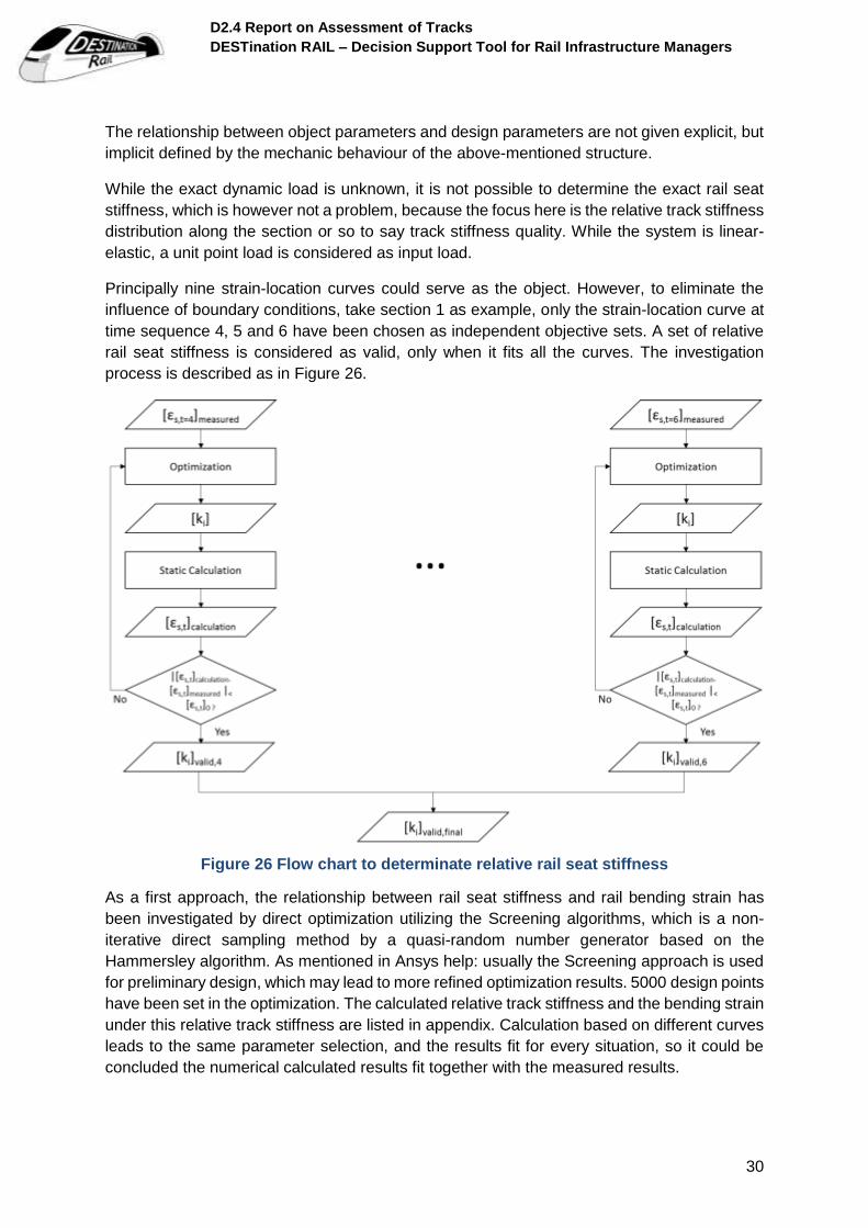
Principally nine strain-location curves could serve as the object. However, to eliminate the
influence of boundary conditions, take section 1 as example, only the strain-location curve at
time sequence 4, 5 and 6 have been chosen as independent objective sets. A set of relative
rail seat stiffness is considered as valid, only when it fits all the curves. The investigation
process is described as in Figure 26.
Figure 26 Flow chart to determinate relative rail seat stiffness
As a first approach, the relationship between rail seat stiffness and rail bending strain has
been investigated by direct optimization utilizing the Screening algorithms, which is a non-
iterative direct sampling method by a quasi-random number generator based on the
Hammersley algorithm. As mentioned in Ansys help: usually the Screening approach is used
for preliminary design, which may lead to more refined optimization results. 5000 design points
have been set in the optimization. The calculated relative track stiffness and the bending strain
under this relative track stiffness are listed in appendix. Calculation based on different curves
leads to the same parameter selection, and the results fit for every situation, so it could be
concluded the numerical calculated results fit together with the measured results.

D2.4 Report on Assessment of Tracks
DESTination RAIL – Decision Support Tool for Rail Infrastructure Managers
31
Under the same way the relative track stiffness at section 2 has been determined, a
comparison of the relative rail seat stiffness at the two sections is showed in Figure 27.
Figure 27 compare of relative track stiffness at location 1 and 2
The variation of track relative stiffness is apparently high at location 1 compared with location
2, which fits the assumption above.
It should be mentioned however, that the relative rail seat stiffness could not be related with
the layer distribution from GPR measurement result directly. While GPR signal could not
penetrate concrete sleepers, GPR could no measure the supporting situation directly
underneath each rail seat. Instead, it measures the position between two rail seats and
extrapolates the measurement result lineally along the measurement section, which indeed
does not fit the situation in reality. In reality, the deterioration directly underneath rail seats
could experience a sudden change compared with the positon between rail seats, while the
traffic load is not distributed equally to the supporting layers by sleepers. So GPR
measurement result could only indicates that the situation of supporting layer is good or bad
in relative long section, it could not identify the exact rail seat stiffness.
3.4 Conclusion
By processing the field measurement results, comparison of loaded and unloaded rail gauge
and cross level enables the synchronization of track recording car measurement to exact track
position. RFID mentioned in proposal is however not applicable for this case.
Besides, the assumption that the difference between loaded and unloaded longitudinal level
is related with dynamic track deflection and further with track stiffness is proved right, which
forms the theoretical background of a new possibility to determine track stiffness.
To study the relationship between loaded and unloaded longitudinal level with track deflection,
multi-body-simulation is implemented in next chapter, which enables the consideration of
dynamic vehicle-track-interaction.

D2.4 Report on Assessment of Tracks
DESTination RAIL – Decision Support Tool for Rail Infrastructure Managers
32
4 Multi-body Simulation
MBS is employed to further study vehicle-track-interaction dynamically. The MBS model has
been implemented in following two aspects:
Parameter determination, which is to determine track stiffness quality given the loaded
and unloaded track longitudinal level. The aim is to develop algorithms to realize the
track stiffness quality monitoring approach established in above chapter.
Evaluation, which is to investigate vehicle-track-system answer under given input
parameters including rail seat stiffness, unloaded track geometry, speed, etc. This
process could be employed to evaluation the influence of certain parameters on track
quality.
For those purposes, a MBS model is established as shown in Figure 28. Besides track
components under the same simplification principal as in FE model, MBS model includes extra
bogie and wheel-rail-contact, which was represented in FE model simply as vertical load. The
wheel-rail-contact model presented in (Blanco-Lorenzo et al., 2011) would be implemented
here.
Figure 28 View of the MBS model
The parameter of the model components are listed below in Table 2.
Table 2 Parameters in the MBS model
Parameter Value
Rail profile S 54 E3
Sleeper profile B 58
Rail pad
Spring constant krp [N/m] 8e8
Damping ratio drp [N*s/m] 1.5e4
Track supporting layer
Spring constant krs [N/m] 2.6e7
Damping ratio drs [N*s/m] 3.1e4
It is here assumed that the variation of track stiffness is only the result of track supporting
layers (ballast layer, sub ballast layer and subgrade) deterioration. Mechanical properties of
D2.4 Report on Assessment of Tracks
DESTination RAIL – Decision Support Tool for Rail Infrastructure Managers
33
other track components including rail, rail pads, rail fastening systems and sleepers are
considered as homogenous distributed along the section the same as the standard value.
4.1 Determination of rail seat stiffness from loaded and unloaded
longitudinal level
Since track deflection is the difference between loaded and unloaded longitudinal level, the
rail seat stiffness would be determined in the simulation by adjusting its value to let the
dynamic track deflection be the same as the difference between loaded and unloaded
longitudinal level at each rail seat. To determine rail seat stiffness, an iteration process is
needed due to the interaction between rail seat stiffness and dynamic wheel-rail-contact load.
Considering the expense of repeating the steps of altering parameters, performing the
calculation and plotting results, a script based on SIMPACK QtScript is written, which realizes
the automation of pre-process, calculation and post-process.
Besides considering the mechanic properties of vehicle-track-components in the numeric
model, the essential part of this method is the iteration algorithms, which determines the speed
of convergence. The algorithms used here is described as followings:
The new rail seat stiffness at position i is defined as
ki,t+1 = ki,t ∗ ( si,t − si,tar
si,t
)2 (6)
with
ki,t – stiffness of rail seat i for iteration step i,
ki,t+1 – stiffness of rail seat i for calculation iteration step i+1,
si,t – deflection of rail seat i at iteration step i.
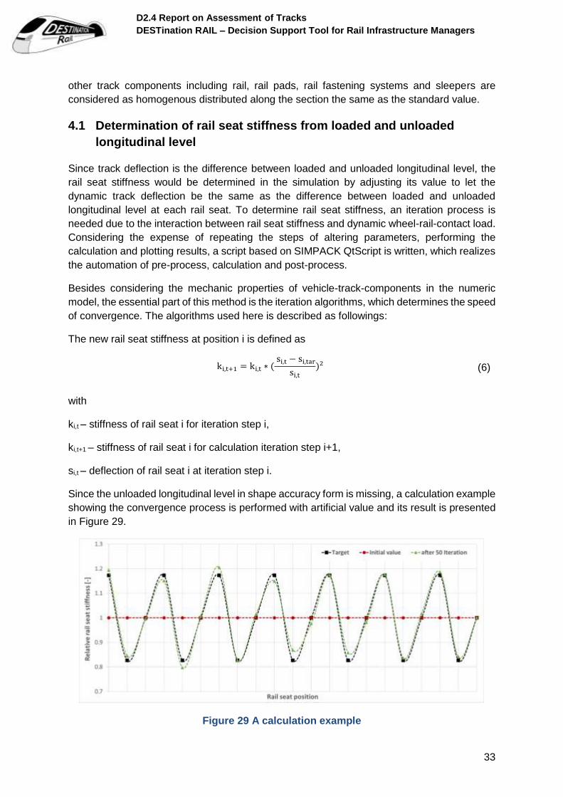
Since the unloaded longitudinal level in shape accuracy form is missing, a calculation example
showing the convergence process is performed with artificial value and its result is presented
in Figure 29.
Figure 29 A calculation example
D2.4 Report on Assessment of Tracks
DESTination RAIL – Decision Support Tool for Rail Infrastructure Managers
34
An artificially defined sinus distribution of rail seat stiffness is given as the object to be achieved.
Starting from equally distributing value, after 50 iterations, the difference between the
predefined sinus rail stiffness the rail seat stiffness determined by the iteration method lies
within a threshold of 5%.
4.2 Evaluation of the influence of track stiffness quality
This MBS model has also been used to study the influence of track stiffness quality on vehicle-
track-system.
Vehicle and track are two sub-systems coupled by wheel-rail-contact, which are excited by
track irregularity and unsteady track deflection simultaneously. Due to the structure of primary
and secondary spring in vehicle, car body and bogie are generally insensible to the excitation
above 20 Hz. In contrast, first Eigen value in vertical track receptance lies in some hundred
hertz (Knothe and Wu, 1998). This difference leads to the division of vehicle-track-interaction
problem into following decoupled categorise according to the interesting frequency level
(Knothe and Grassie, 1993, Popp et al., 1999):
Problems of Vehicle Dynamics, vehicle stability and passenger comfort. Below 20 Hz.
Problems Involving Components of the Bogie and Unsprung Mass, elastic deformation
of the wheelset. 10 - 50 Hz
Deterioration of track components and track bed, 50 – 500 Hz.
Noise, up to 5 kHz.
Since the focus here lies in the performance of track in vehicle-track-interaction, the modelling
of car body is not necessary. In this study, only bogie has been built in the numeric model to
represent vehicle. In contrast, the track component has been modelled in detail.
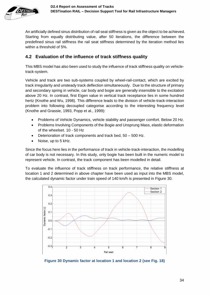
To evaluate the influence of track stiffness on track performance, the relative stiffness at
location 1 and 2 determined in above chapter have been used as input into the MBS model,
the calculated dynamic factor under train speed of 140 km/h is presented in Figure 30.
Figure 30 Dynamic factor at location 1 and location 2 (see Fig. 18)

D2.4 Report on Assessment of Tracks
DESTination RAIL – Decision Support Tool for Rail Infrastructure Managers
35
The dynamic factor η is defined as:
η = 𝐹𝑑𝑦𝑛 − 𝐹𝑠𝑡𝑎𝑡
𝐹𝑠𝑡𝑎𝑡
(7)
Where
Fdyn is the real time dynamic force introduced on track,
Fstat is the static load caused by the self-weight of vehicle.
It could be observed that the maximal dynamic factor at location 1 is 0.34, whereas the
dynamic factor at location 2 stay below 0.10, which shows the influence of track stiffness
quality on track performance.
4.3 Comparison of the influence of track stiffness quality and track
geometry quality
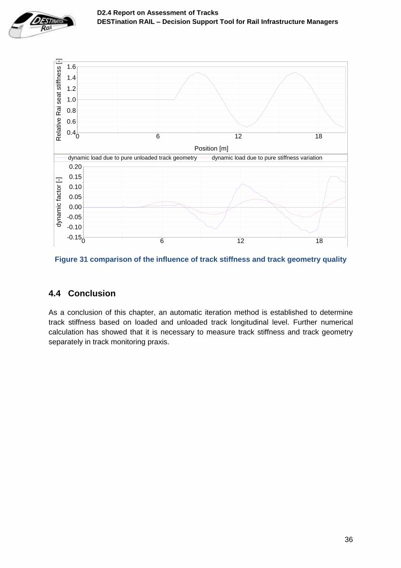
In this chapter, the influence of track stiffness quality on track performance is compared with
the influence of track geometry quality. Two scenarios have been defined. In scenario one,
only an artificially defined track stiffness variation has been imported into the MBS model as
trackside excitation. In scenario two, the wheelset deflection determined in scenario one is
plotted and imported here as unloaded track irregularity into the model. Track components in
scenario two have been switch to rigid to eliminate the influence of track stiffness.
Comparing these two scenarios, the measured loaded track geometry should be the same
when TRC runs by. However, the determined dynamic load shows apparently difference,
which is presented in Figure 31. The influence of track geometry is greater as track stiffness,
under the condition that they are of the same amplitude.
From this point of view, the traditional track monitoring method using TRC measurement
results could lead to overestimate of the severity of track quality problems, separated
consideration of track stiffness and track geometry could lead to more accurate evaluation.
D2.4 Report on Assessment of Tracks
DESTination RAIL – Decision Support Tool for Rail Infrastructure Managers
36
Figure 31 comparison of the influence of track stiffness and track geometry quality
4.4 Conclusion
As a conclusion of this chapter, an automatic iteration method is established to determine
track stiffness based on loaded and unloaded track longitudinal level. Further numerical
calculation has showed that it is necessary to measure track stiffness and track geometry
separately in track monitoring praxis.
dynamic load due to pure unloaded track geometry dynamic load due to pure stiffness variation
Position [m]
0 6 12 18Re
lative
Ra
i se
at
stiff
ne
ss [
-]
0.4
0.6
0.8
1.0
1.2
1.4
1.6
0 6 12 18
dyn
am
ic f
acto
r [-
]
-0.15
-0.10
-0.05
0.00
0.05
0.10
0.15
0.20
D2.4 Report on Assessment of Tracks
DESTination RAIL – Decision Support Tool for Rail Infrastructure Managers
37
5 Conclusion and Outlook
In this research, it is concluded that the difference between loaded and unloaded longitudinal
level is related with track supporting layer stiffness variation, which could be revealed by GPR
measurement.
By comparing rail gauge and cross level from loaded and unloaded track geometry, the
measurement result from track recording car could be exactly synchronized to rail seat. RFID
is at present not suitable for this task.
Numerical methods have been developed which could not only determine track stiffness
variation in short section based on track borne measurement results (rail bending strain), but
also could determine track stiffness variation in long section based on train borne
measurement result (loaded and unloaded longitudinal level).
Finally based on numerical simulation, influence of track stiffness on track quality has been
investigated. It is especially pointed out, compared with loaded track geometry that is currently
widely used in track monitoring praxis, a separate consideration of unloaded track geometry
and track stiffness describes track quality more accurately.
The research could be furtherly improved when following items could be realised:
Employ capable unloaded track geometry equipment to acquired shape accuracy track
geometry, for example as mentioned in (Schmeister, 2013),
Perform GPR measurement more sophisticatedly, which not only measures the layer
distribution, but also provides detailed information about moisture content and ballast
fouling index etc., for example as shown in (Levomaki et al., 2010),
Detailed information of vehicle (RAILab, Meridian and BOB).
D2.4 Report on Assessment of Tracks
DESTination RAIL – Decision Support Tool for Rail Infrastructure Managers
38
6 Reference
BERG, M., BERGGREN, E. G. & LI, M. X. D. 2009. Assessment of vertical track geometry quality based on simulations of dynamic track–vehicle interaction. Proceedings of the Institution of Mechanical Engineers, Part F: Journal of Rail and Rapid Transit, 223, 131-139.
BERGGREN, E. G. 2009. Railway Track Stiffness : Dynamic Measurements and Evaluation for Efficient Maintenance. 2009:17, KTH.
BLANCO-LORENZO, J., SANTAMARIA, J., VADILLO, E. G. & OYARZABAL, O. 2011. Dynamic comparison of different types of slab track and ballasted track using a flexible track model. Proceedings of the Institution of Mechanical Engineers, Part F: Journal of Rail and Rapid Transit, 225, 574-592.
CLARK, M., GORDON, M. & FORDE, M. C. 2004. Issues over high-speed non-invasive monitoring of railway trackbed. NDT & E International, 37, 131–139.
DE BOLD, R., O’CONNOR, G., MORRISSEY, J. P. & FORDE, M. C. 2015. Benchmarking large scale GPR experiments on railway ballast. Construction and Building Materials, 92, 31-42.
HAIGERMOSER, A., LUBER, B., RAUH, J. & GRÄFE, G. 2015. Road and track irregularities: measurement, assessment and simulation. Vehicle System Dynamics, 53, 878-957.
IWNICKI, S. 2006. Handbook of railway vehicle dynamics, CRC press. KIPPER, R., GERBER, U. & SCHMEISTER, J. 2013. Bestimmung langwelliger
Gleisverformungen und deren Bewertung. EI Der Eisenbahningenieur, 11-16. KNOTHE, K. L. & GRASSIE, S. L. 1993. Modelling of Railway Track and Vehicle/Track
Interaction at High Frequencies. Vehicle System Dynamics, 22, 209-262. KNOTHE, K. L. & STICHEL, S. 2003. Schienenfahrzeugdynamik, Springer. KNOTHE, K. L. & WU, Y. 1998. Receptance behaviour of railway track and subgrade. Archive
of Applied Mechanics, 68, 457-470. KRUGLIKOV, A., YAVNA, V., LAZORENKO, G. & KHAKIEV, Z. Investigation of long term
moisture changes in roadbeds using GPR. Ground Penetrating Radar (GPR), 2014 15th International Conference on, 2014. IEEE, 857-861.
LEVOMAKI, M., WILJANEN, B., NURMIKOLU, A. & SILVAST, M. 2010. An inspection of railway ballast quality using ground penetrating radar in Finland. Proceedings of the Institution of Mechanical Engineers, Part F: Journal of Rail and Rapid Transit, 224, 345-351.
LIU, D. 2015. The influence of track quality to the performance of vehicle-track interaction. München, Technische Universität München, Diss., 2015.
PAIXÃO, A., FORTUNATO, E. & CALÇADA, R. 2016. A contribution for integrated analysis of railway track performance at transition zones and other discontinuities. Construction and Building Materials, 111, 699-709.
POPP, K., KRUSE, H. & KAISER, I. 1999. Vehicle-Track Dynamics in the Mid-Frequency Range. Vehicle System Dynamics, 31, 423-464.
ROGHANI, A. & HENDRY, M. T. 2016. Continuous Vertical Track Deflection Measurements to Map Subgrade Condition along a Railway Line: Methodology and Case Studies. Journal of Transportation Engineering, 142, 04016059.
SCHMEISTER, J. 2013. Vergleichsmessung RPIRAILab. SILVAST, M., NURMIKOLU, A., WILJANEN, B. & LEVOMÄKI, M. Inspection of railway ballast
quality using GPR in Finland. 9th International Heavy Haul Conference, Shanghai, China, June 22-25, 2009, 2009.
SU, L., INDRARATNA, B. & RUJIKIATKAMJORN, C. 2011. Non-destructive assessment of rail track condition using ground penetrating radar.
WANG, P., WANG, L., CHEN, R., XU, J., XU, J. & GAO, M. 2016. Overview and outlook on railway track stiffness measurement. Journal of Modern Transportation, 24, 89-102.
D2.4 Report on Assessment of Tracks
DESTination RAIL – Decision Support Tool for Rail Infrastructure Managers
39
WOLTER, C. U. 2013. Rekonstruktion der originalen Gleislageabweichungen aus 3-Punkt-Signalen (Wandersehnenmessverfahren) und Beurteilung hinsichtlich Amplitude, Fehlerwellenlänge sowie Fehlerform, Eurailpress in DVV Media Group.
WU, X., CAI, W., CHI, M., WEI, L., SHI, H. & ZHU, M. 2015. Investigation of the effects of sleeper-passing impacts on the high-speed train. Vehicle System Dynamics, 53, 1902-1917.
ZHANG, Y., VENKATACHALAM, A. S. & XIA, T. 2015. Ground-penetrating radar railroad ballast inspection with an unsupervised algorithm to boost the region of interest detection efficiency. Journal of Applied Remote Sensing, 9, 095058-095058.
D2.4 Report on Assessment of Tracks
DESTination RAIL – Decision Support Tool for Rail Infrastructure Managers
40
Appendix A
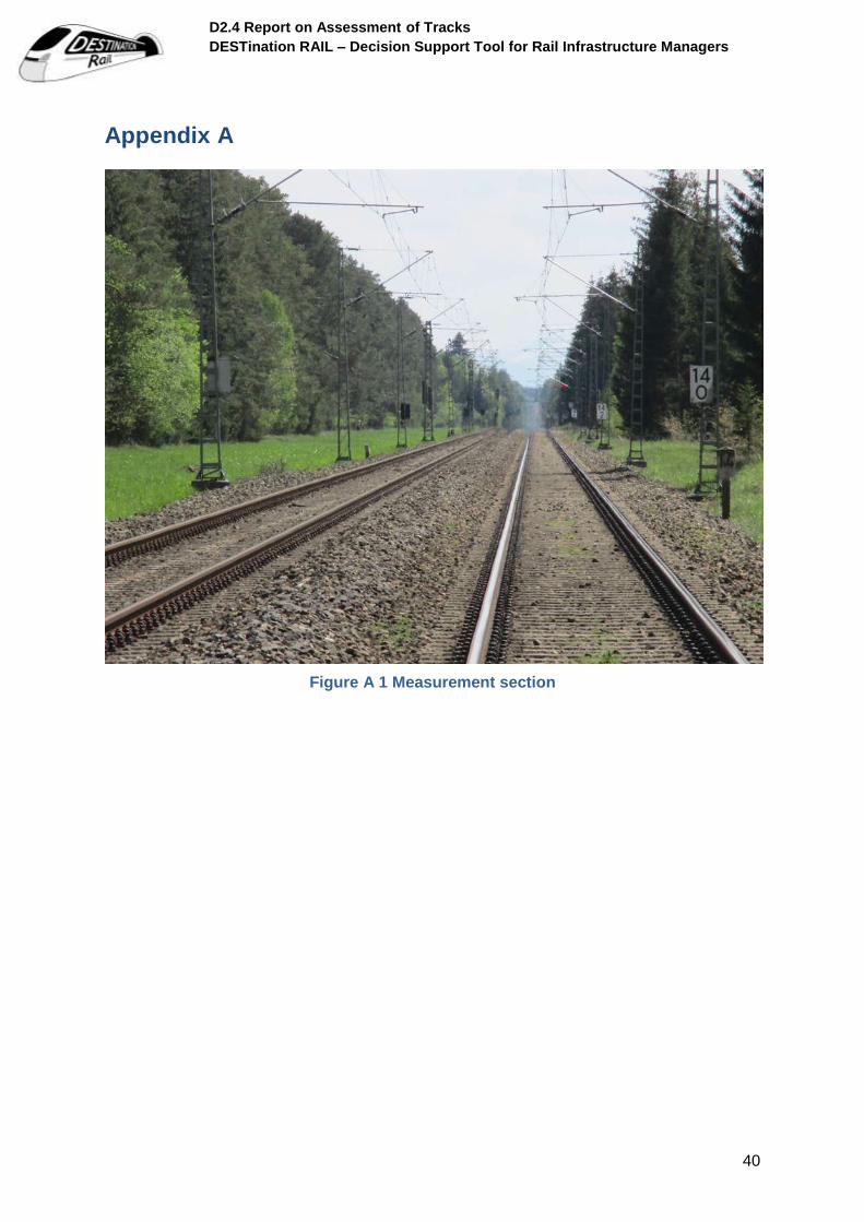
Figure A 1 Measurement section

D2.4 Report on Assessment of Tracks
DESTination RAIL – Decision Support Tool for Rail Infrastructure Managers
41
Figure A 2 Comparison of track gauge

D2.4 Report on Assessment of Tracks
DESTination RAIL – Decision Support Tool for Rail Infrastructure Managers
42
Figure A 3 GPR measurement equipment
D2.4 Report on Assessment of Tracks
DESTination RAIL – Decision Support Tool for Rail Infrastructure Managers
43
Figure A 4 Output from GPR
D2.4 Report on Assessment of Tracks
DESTination RAIL – Decision Support Tool for Rail Infrastructure Managers
44
Figure A 5 Build of measurement
D2.4 Report on Assessment of Tracks
DESTination RAIL – Decision Support Tool for Rail Infrastructure Managers
45
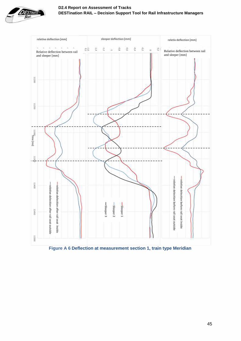
Figure A 6 Deflection at measurement section 1, train type Meridian
Relative deflection between rail
and sleeper [mm] Relative deflection between rail
and sleeper [mm]
D2.4 Report on Assessment of Tracks
DESTination RAIL – Decision Support Tool for Rail Infrastructure Managers
46
Figure A 7 Rail bending strain at measurement section 1, train type Meridian
D2.4 Report on Assessment of Tracks
DESTination RAIL – Decision Support Tool for Rail Infrastructure Managers
47
Figure A 8 Deflection at measurement section 2, train type Meridian
Relative deflection between rail
and sleeper [mm]
Relative deflection between rail
and sleeper [mm]
D2.4 Report on Assessment of Tracks
DESTination RAIL – Decision Support Tool for Rail Infrastructure Managers
48
Figure A 9 Rail bending strain at measurement section 2, train type Meridian
D2.4 Report on Assessment of Tracks
DESTination RAIL – Decision Support Tool for Rail Infrastructure Managers
49
Figure A 10 Deflection at measurement section 1, train type BOB
Relative deflection between rail
and sleeper [mm] Relative deflection between rail and sleeper [mm]

D2.4 Report on Assessment of Tracks
DESTination RAIL – Decision Support Tool for Rail Infrastructure Managers
50
Figure A 11 Rail bending strain at measurement section 1, train type BOB
D2.4 Report on Assessment of Tracks
DESTination RAIL – Decision Support Tool for Rail Infrastructure Managers
51
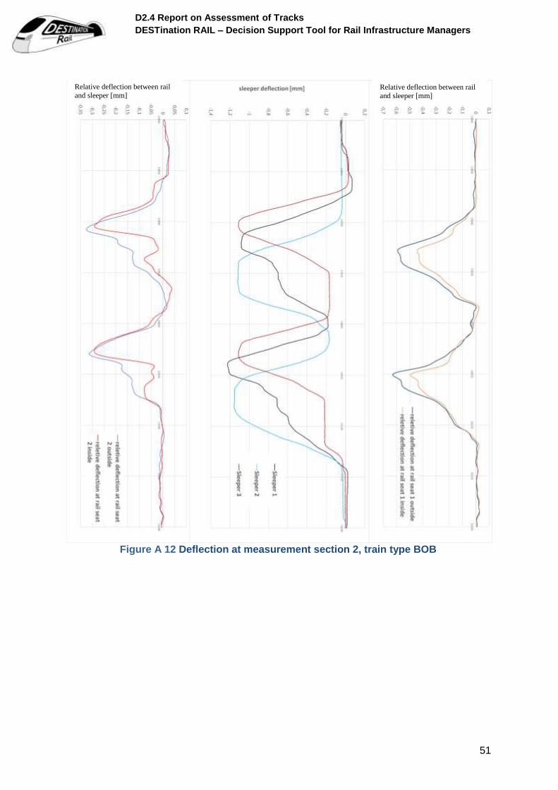
Figure A 12 Deflection at measurement section 2, train type BOB
Relative deflection between rail
and sleeper [mm] Relative deflection between rail
and sleeper [mm]
D2.4 Report on Assessment of Tracks
DESTination RAIL – Decision Support Tool for Rail Infrastructure Managers
52
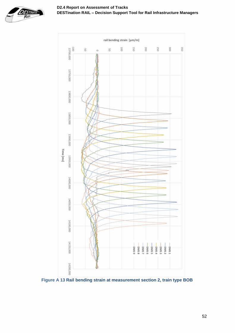
Figure A 13 Rail bending strain at measurement section 2, train type BOB

D2.4 Report on Assessment of Tracks
DESTination RAIL – Decision Support Tool for Rail Infrastructure Managers
53
Table A 1 Measured strain with respect to time and location [kN∙m]
load measure
6900 7500 8100 8700 9300 9900 10500 11100 11700
6900 -13,98 -1,21 1,48 1,69 0,98 0,70 -0,17 -0,32 -0,22
7500 0,25 -15,59 0,01 2,01 1,77 1,13 0,08 -0,38 -0,24
8100 3,50 -0,12 -15,07 -0,15 2,08 1,64 0,86 0,02 0,17
8700 0,58 3,43 1,45 -14,77 -0,70 1,22 1,36 1,12 0,41
9300 -12,58 0,78 5,09 1,96 -16,06 -2,52 1,94 2,30 1,43
9900 -0,86 -14,72 3,29 4,80 -1,34 -14,24 0,43 3,17 2,28
10500 1,35 -1,15 -13,44 2,69 2,74 -0,18 -12,26 2,12 2,64
11100 1,45 1,78 0,42 -13,04 0,06 2,69 1,45 -11,99 1,17
11700 1,17 1,96 2,28 -0,35 -16,65 -1,41 4,22 2,79 -12,31
Table A 2 Calculated strain with respect to time and location [kN∙m]
load measure
6900 7500 8100 8700 9300 9900 10500 11100 11700
6900 -13,53 1,91 1,19 0,06 -0,08 -0,04 0,00 0,00 0,00
7500 1,06 -12,46 2,76 0,44 -0,10 -0,10 -0,01 0,00 0,00
8100 0,33 3,33 -12,61 0,21 1,09 0,38 -0,02 -0,02 0,00
8700 1,02 3,16 2,75 -15,64 0,53 2,37 0,55 -0,08 -0,02
9300 -13,57 2,40 3,64 0,86 -15,93 2,43 2,25 0,05 -0,05
9900 1,05 -12,50 3,19 1,82 0,35 -13,52 2,89 0,90 -0,02
10500 0,33 3,30 -12,68 0,29 1,82 1,86 -12,34 2,30 0,43
11100 0,01 2,21 2,68 -15,68 0,50 2,83 3,20 -12,84 0,99
11700 -0,03 0,49 2,44 0,78 -15,90 2,48 3,37 1,07 -12,92
Table A 3 Compare [%]
load measure
6900 7500 8100 8700 9300 9900 10500 11100 11700
6900 -3 -258 -19 -96 -108 -106 -99 -101 -100
7500 333 -20 20445 -78 -106 -109 -118 -101 -100
8100 -91 -2828 -16 -243 -47 -77 -102 -230 -100
8700 77 -8 89 6 -176 94 -60 -107 -104
9300 8 207 -29 -56 -1 -196 16 -98 -104
9900 -222 -15 -3 -62 -127 -5 569 -72 -101
10500 -76 -387 -6 -89 -33 -1123 1 8 -84
11100 -100 24 539 20 715 5 121 7 -15
11700 -103 -75 7 -320 -5 -276 -20 -62 5

D2.4 Report on Assessment of Tracks
DESTination RAIL – Decision Support Tool for Rail Infrastructure Managers
54
Figure A 14 compare measurement and simulation_ B_1_strain-time curve

D2.4 Report on Assessment of Tracks
DESTination RAIL – Decision Support Tool for Rail Infrastructure Managers
55
Figure A 15 Compare measurement and simulation_ B_1_strain-location curve

D2.4 Report on Assessment of Tracks
DESTination RAIL – Decision Support Tool for Rail Infrastructure Managers
56
Figure A 16 Compare measurement and simulation_ M_1_strain-time curve
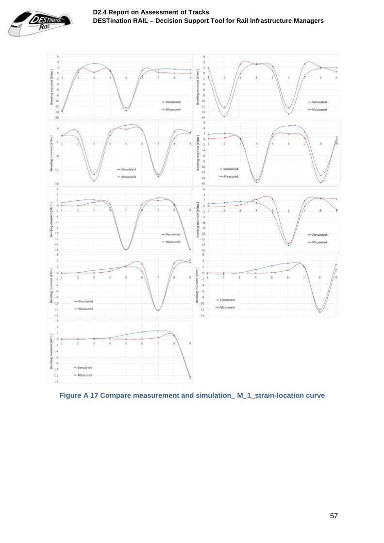
D2.4 Report on Assessment of Tracks
DESTination RAIL – Decision Support Tool for Rail Infrastructure Managers
57
Figure A 17 Compare measurement and simulation_ M_1_strain-location curve