replication, statistical consistency, and publication biasgfrancis/publications/francis2013b.pdf ·...
TRANSCRIPT

Replication, statistical consistency, and publication bias
Gregory Francis1
Department of Psychological Sciences
Purdue University
703 Third Street
West Lafayette, IN 47907-2004
November 8, 2012
Revised: February 13, 2013
Key words: Hypothesis testing, statistics, publication bias, scientific publishing
Running head: Statistical consistency and publication bias
1E-mail: [email protected]; phone: 765-494-6934.
Abstract
Scientific methods of investigation o↵er systematic ways to gather information about the world;
and in the field of psychology application of such methods should lead to a better understanding
of human behavior. Instead, recent reports in psychological science have used apparently scientific
methods to report strong evidence for unbelievable claims such as precognition. To try to resolve
the apparent conflict between unbelievable claims and the scientific method many researchers turn
to empirical replication to reveal the truth. Such an approach relies on the belief that true phe-
nomena can be successfully demonstrated in well-designed experiments, and the ability to reliably
reproduce an experimental outcome is widely considered the gold standard of scientific investiga-
tions. Unfortunately, this view is incorrect; and misunderstandings about replication contribute to
the conflicts in psychological science. Because experimental e↵ects in psychology are measured by
statistics, there should almost always be some variability in the reported outcomes. An absence of
such variability actually indicates that experimental replications are invalid, perhaps because of a
bias to suppress contrary findings or because the experiments were run improperly. Recent inves-
tigations have demonstrated how to identify evidence of such invalid experiment sets and noted its
appearance for prominent findings in experimental psychology. The present manuscript explores
those investigative methods by using computer simulations to demonstrate their properties and lim-
itations. The methods are shown to be a check on the statistical consistency of a set of experiments
by comparing the reported power of the experiments with the reported frequency of statistical
significance. Overall, the methods are extremely conservative about reporting inconsistency when
experiments are run properly and reported fully. The manuscript also considers how to improve
scientific practice to avoid inconsistency, and discusses criticisms of the investigative method.

Statistical consistency and publication bias 3
1 Introduction
“At the heart of science is an essential balance between two seemingly contradictory attitudes–
an openness to new ideas, no matter how bizarre or counterintuitive they may be, and the most
ruthless skeptical scrutiny of all ideas, old and new. This is how deep truths are winnowed from
deep nonsense.” Carl Sagan (1997).
The field of psychology certainly follows the first half of Sagan’s prescription for scientific
investigations, as evidenced by the many creative and counterintuitive experimental descriptions of
human behavior. This article is about the second half of the prescription, which calls for ruthless
skeptical scrutiny of all ideas. The need for skeptical scrutiny was highlighted by Bem’s (2011)
reported evidence of human precognition (the ability to acquire information from the future).
Bem’s experimental methods did not appear to be substantively di↵erent from other studies, and
with nine out of ten findings reporting evidence for precognition (by rejecting the null hypothesis),
the findings in Bem (2011) exceeded what is normally required of psychological investigations. The
apparently high quality of Bem’s studies presented a quandary for researchers who do not believe in
precognition (as it would require fundamental modifications to theories of physics, chemistry, and
biology) because their disbelief required that there be some unknown flaw with Bem’s investigations,
and such a flaw might also be present in investigations of other (more believable) topics. For these
reasons some researchers have suggested that experimental psychology faces a crisis (e.g., Pashler &
Wagenmakers, 2012; Shea, 2011; Wagenmakers, Wetzels, Borsboom, & van der Maas, 2011; Yong,
2012a).
The field does face a crisis, there is such a flaw, and it does apply to other topics. The flaw
is related to misunderstandings about what is widely considered the gold standard for empirical
work: replication. Empirical replication is widely considered to be a cornerstone of science. Many
researchers responding to Bem’s findings and related controversies emphasize that experimental
replication will ultimately demonstrate the truth (e.g., Ritchie, Wiseman & French, 2012; Roediger,
2012; Galak, LeBoeuf, Nelson & Simmons, 2012). There is much value to repeating experiments,
but there are fundamental misunderstandings about the properties of replication. For example,
it is possible to have too much successful replication. Since experiments in psychology depend
on random sampling, they should sometimes fail to reject a false null hypothesis; thus too many
successful replications can be “too good to be true.” Francis (2012a) showed that such was the
Statistical consistency and publication bias 4
case for Bem’s precognition studies.
As described in detail below, the absence of null findings can indicate the presence of publication
bias, where authors (perhaps encouraged by editors or reviewers) suppressed null findings. Another
explanation for too much replication success is that authors used questionable research practices or
analysis methods (Simmons, Nelson & Simonsohn, 2011; John, Lowenstein & Prelec, 2012) in a way
that increased the rejection rate of their experiments. The analysis is based on a test for an excess
of significant findings proposed by Ioannidis and Trikalinos (2007), which detects the presence of
some of these problems. Schimmack (2012) used similar calculations to compute an “incredibility”
index. Francis (2012a–g, 2013) used the test to detect publication bias in several studies. As shown
below, these analytical methods are best described as an investigation of statistical consistency for
reported experimental results.
2 Statistical consistency as a test for publication bias
Ioannidis and Trikalinos (2007) proposed using reported e↵ect sizes to estimate the power of each
experiment and then using those power measures to predict how often one would expect to reject
the null hypothesis. If the number of observed rejections is substantially larger than what was
expected, then the test indicates evidence for an excess of significant findings. In essence, the test
checks on the internal consistency of the number of reported significant findings, the reported e↵ect
size, and the power of the tests to detect that e↵ect size.
A di↵erence between the expected and observed number of experiments that reject the null
hypothesis can be analyzed with a �2 test:
�2(1) =(O � E)2
E+
(O � E)2
M � E, (1)
where O and E refer to the observed and expected number of studies that reject the null hypothesis,
and M is the total number of studies in the set of experiments. O is easily counted as the number
of reported experiments that reject the null hypothesis. For a set of M independent experiments
with Type II error values �i, the expected number of times the set of experiments would reject the
null hypothesis is
E =MX
i=1
(1� �i) , (2)
which simply adds up the power values across the experiments. As described below, the calculation
of the �i and power values depends on the properties and interpretation of the experiments.
Statistical consistency and publication bias 5
To compute the probability of getting a particular pattern of rejections for a given set of exper-
iments, create a binary vector, a = [a(1),. . . , a(M)], that indicates whether each of M experiments
rejects the null hypothesis (1) or not (0). The probability of a particular pattern of rejections and
non-rejections can be computed from the power and Type II error values:
Prob(a) =MY
i=1
(1� �i)a(i) �(1�a(i))i (3)
The equation is simply the product of the power and Type II error values for the experiments that
reject the null hypothesis or fail to reject the null hypothesis, respectively. If every experiment
rejects the null hypothesis, the term will simply be the product of all the power values.
For small experiment sets, the �2 test can be replaced by Fisher’s exact test to compute the
probability of the observed number of rejections, O, or more rejections. If the vectors that describe
di↵erent combinations of experiments are designated by a subscript, j, then the probability of a
set of experiments having O or more rejections out of a set of M experiments is:
Pc = Prob(� O experiments reject) =MX
k=O
MCkX
j=1
Prob(aj), (4)
where MCk indicates M choose k, the number of di↵erent combinations of k rejections from a set of
M experiments, and j indexes those di↵erent combinations. If all of the experiments in a reported
set reject the null hypothesis, then there is only one term under the summations, and equation (4)
becomes the product of the power values. If the Pc value is small, then the analysis concludes that
the set of experiments appears to be inconsistent. It is somewhat arbitrary, but tests of publication
bias frequently use a criterion of 0.1 (Begg & Mazumdar, 1994; Ioannidis & Trikalinos, 2007; Sterne,
Gavaghan & Egger, 2000).
In essence, the test investigates whether the observed rate of rejecting the null hypothesis is
consistent with the rate that should be produced for the measured e↵ect size and the experiment
sample sizes. If these rates are quite di↵erent, then there appears to be something wrong with
the experiments or their reporting. As such, the test is not a direct investigation of publication
bias, but a check on the “consistency” of the reported results. As shown below, various forms of
publication bias sometimes inflate the occurrence of inconsistency.
A critical issue for a test of consistency is the calculation of the �i (and power) terms in equation
(3). If the true e↵ect size is known, then power is easily computed using non-central t distributions
(Cohen, 1988; Champley, 2010). As an introduction to the basic ideas of the consistency test, it

Statistical consistency and publication bias 6
is useful to consider a two-sample t-test where the true standardized e↵ect size between the null
and alternative (normally distributed) populations is � = 0.5. If the test has equal sample sizes
of n1 = n2 = 32, then the true power of each experiment is approximately 0.5. Suppose there is
a set of M = 10 such tests. (All of the simulations in this article use two-sample t-tests, but the
logic applies for other analyses as well.) One would expect to observe around five rejections of
the null hypothesis from the set of ten tests, with variability in the number of rejections described
by a binomial distribution. If all experiments are run properly and reported fully, the consistency
test will reject the null hypothesis when eight or more experiments out of the ten reject the null
hypothesis. The binomial distribution indicates that such cases will happen with a probability of
0.0547. It is worth noting that even though the criterion for the consistency test is 0.1, the actually
observed Type I error rate is usually smaller because of the discrete nature of the observations.
When experiments vary in sample size it becomes di�cult to characterize the rule for consis-
tency in an analytic way, so the properties of the consistency test were explored with computer
simulations. Consider a two-sample t-test where the true standardized e↵ect size between the null
and alternative (normally distributed) populations with standard deviations of one is � = 0.5. In
each experiment the sample sizes were an equal (n1 = n2) whole number picked randomly from a
uniform distribution across the interval (22, 42). At the median sample size of 32, such experiments
would have a power value of approximately 0.5. When there are M = 10 experiments in a set,
one would expect to observe a bit fewer than five rejections of the null hypothesis (power is not
symmetric with variation in sample size), but the actual number will depend on the properties of
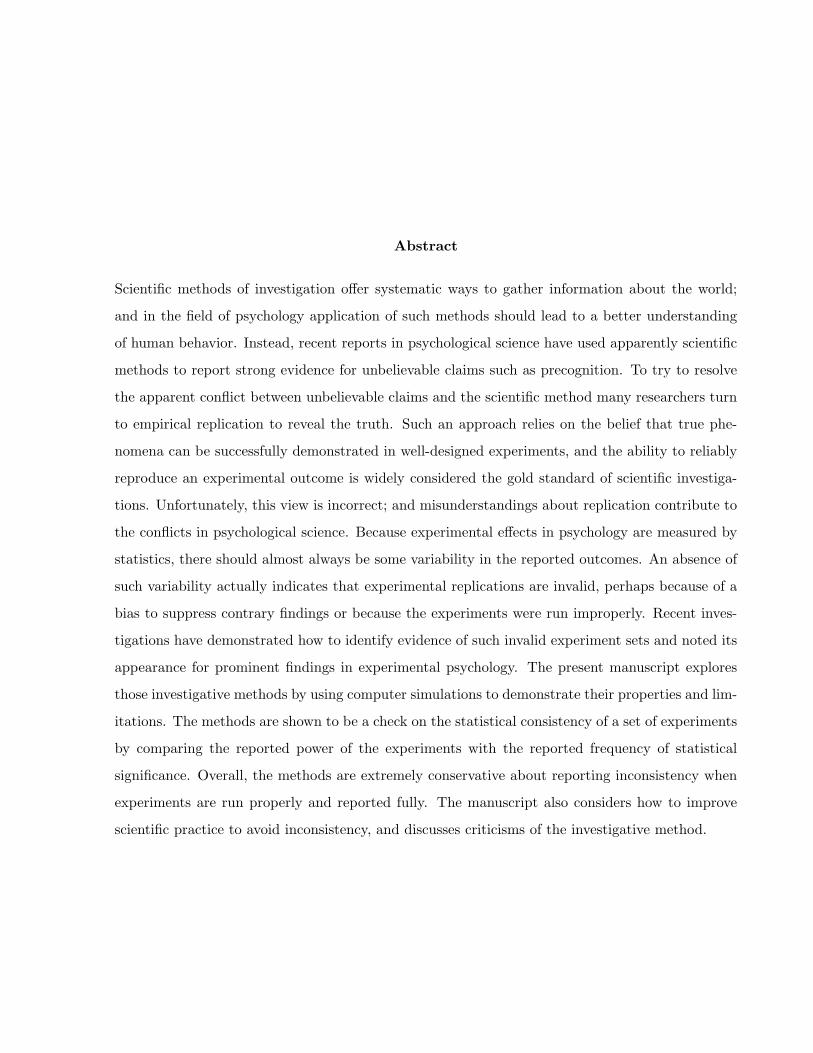
the sampled data. Figure 1A plots a frequency distribution of the observed number of rejections
of the null hypothesis. The distribution is similar to a binomial distribution, but deviates slightly
because the power of the experiments is not constant. For the properties of these experiments, it
would be very uncommon to observe (p = 0.046) eight or more rejections of the null hypothesis out
of a set of ten experiments.
The consistency test based on the true e↵ect size was applied to 1000 simulated experiment
sets. Since the number of experiments in a set was fairly small, the exact test in equation (4)
was used. An experiment set was judged to be “inconsistent” if Pc 0.1, while experiment sets
that had Pc > 0.1 were termed “consistent.” As shown in Figure 1A, these experiment sets are
generally inconsistent relative to the true e↵ect size when eight or more experiments reject the
null hypothesis. Because of variations in the sample sizes of experiments, sometimes experiment
Statistical consistency and publication bias 7
6 6 8 8 8Number of observed rejections
-0.2
0
0.2
0.4
0.6
0.8
1
1.2
Effe
ct s
ize
Inconsistent experiment sets
3 4 5 6 7Number of observed rejections
-0.2
0
0.2
0.4
0.6
0.8
1
1.2
Effe
ct s
ize
Consistent experiment sets
0.2 0.4 0.6 0.8 1Pooled effect size
0
2
4
6
8
10
Obs
erve
d nu
mbe
r of r
ejec
tions
ConsistentTrue ES inconsistentPooled ES inconsistent
B
C D
0 2 4 6 8 10Observed number of rejections
0
50
100
150
200
250
Freq
uenc
y
Inconsistent setsConsistent setsA
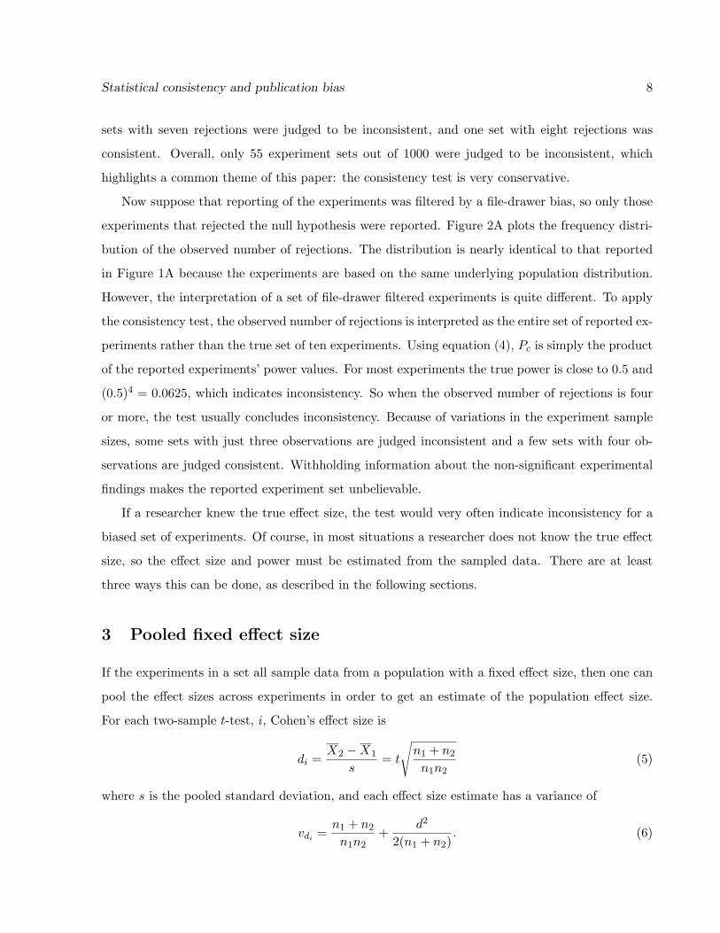
Figure 1: Explorations of the consistency test when all simulated experiments are run properly
and reported fully. Panel A shows a frequency distribution of the observed number of rejections,
which is similar to a binomial distribution. The classification of consistent and inconsistent sets
is relative to the true e↵ect size. In panel B each point corresponds to a set of ten experiments.
The light diamonds indicate experiment sets that were judged consistent. The circles indicate sets
that are judged inconsistent relative to the true e↵ect size. The X’s indicate sets that are judged
inconsistent relative to the pooled fixed e↵ect size. The latter cases are very rare. Panel C shows
the experiment-wise e↵ect sizes (circles) and pooled e↵ect size for the five experiment sets in B that
are judged to be inconsistent with the pooled e↵ect size. Panel D shows the experiment-wise e↵ect
sizes and pooled e↵ect size for five representative experiments that are judged to be consistent with
the pooled e↵ect size.
Statistical consistency and publication bias 8
sets with seven rejections were judged to be inconsistent, and one set with eight rejections was
consistent. Overall, only 55 experiment sets out of 1000 were judged to be inconsistent, which
highlights a common theme of this paper: the consistency test is very conservative.
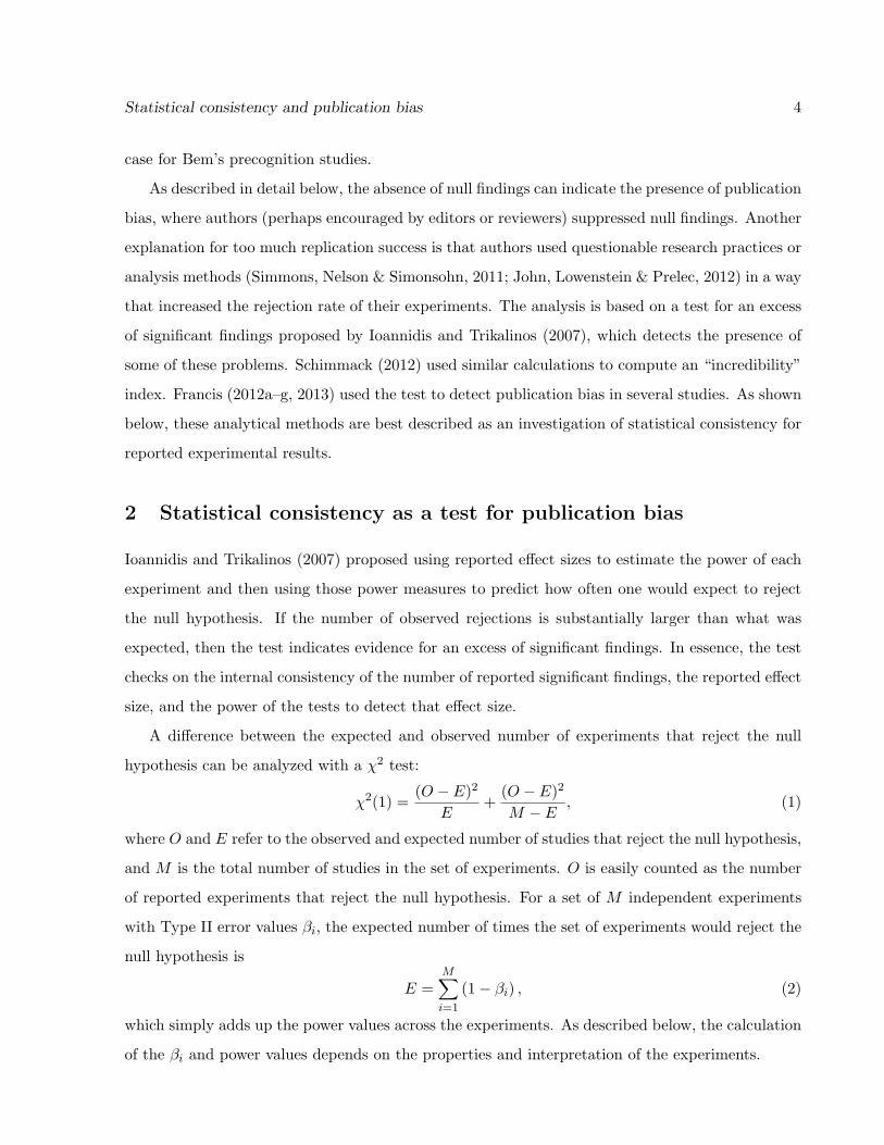
Now suppose that reporting of the experiments was filtered by a file-drawer bias, so only those
experiments that rejected the null hypothesis were reported. Figure 2A plots the frequency distri-
bution of the observed number of rejections. The distribution is nearly identical to that reported
in Figure 1A because the experiments are based on the same underlying population distribution.
However, the interpretation of a set of file-drawer filtered experiments is quite di↵erent. To apply
the consistency test, the observed number of rejections is interpreted as the entire set of reported ex-
periments rather than the true set of ten experiments. Using equation (4), Pc is simply the product
of the reported experiments’ power values. For most experiments the true power is close to 0.5 and
(0.5)4 = 0.0625, which indicates inconsistency. So when the observed number of rejections is four
or more, the test usually concludes inconsistency. Because of variations in the experiment sample
sizes, some sets with just three observations are judged inconsistent and a few sets with four ob-
servations are judged consistent. Withholding information about the non-significant experimental
findings makes the reported experiment set unbelievable.
If a researcher knew the true e↵ect size, the test would very often indicate inconsistency for a
biased set of experiments. Of course, in most situations a researcher does not know the true e↵ect
size, so the e↵ect size and power must be estimated from the sampled data. There are at least
three ways this can be done, as described in the following sections.
3 Pooled fixed e↵ect size
If the experiments in a set all sample data from a population with a fixed e↵ect size, then one can
pool the e↵ect sizes across experiments in order to get an estimate of the population e↵ect size.
For each two-sample t-test, i, Cohen’s e↵ect size is
di =X2 �X1
s= t
sn1 + n2
n1n2(5)
where s is the pooled standard deviation, and each e↵ect size estimate has a variance of
vdi =n1 + n2
n1n2+
d2
2(n1 + n2). (6)
Statistical consistency and publication bias 9
0.2 0.4 0.6 0.8 1Pooled effect size
0
2
4
6
8
10
Obs
erve
d nu
mbe
r of r
ejec
tions
ConsistentTrue ES inconsistentFixed ES inconsistent
5 6 7 8 9Observed number of rejections
-0.2
0
0.2
0.4
0.6
0.8
1
1.2
Effe
ct s
ize
Inconsistent experiment sets
3 4 5 7 9Observed number of rejections
-0.2
0
0.2
0.4
0.6
0.8
1
1.2
Effe
ct s
ize
Consistent experiment sets
B
C D
0 2 4 6 8 10Observed number of rejections
0
50
100
150
200
250
Freq
uenc
y
Inconsistent setsConsistent setsA
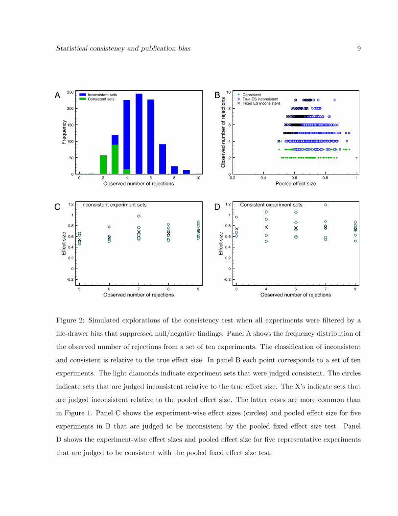
Figure 2: Simulated explorations of the consistency test when all experiments were filtered by a
file-drawer bias that suppressed null/negative findings. Panel A shows the frequency distribution of
the observed number of rejections from a set of ten experiments. The classification of inconsistent
and consistent is relative to the true e↵ect size. In panel B each point corresponds to a set of ten
experiments. The light diamonds indicate experiment sets that were judged consistent. The circles
indicate sets that are judged inconsistent relative to the true e↵ect size. The X’s indicate sets that
are judged inconsistent relative to the pooled e↵ect size. The latter cases are more common than
in Figure 1. Panel C shows the experiment-wise e↵ect sizes (circles) and pooled e↵ect size for five
experiments in B that are judged to be inconsistent by the pooled fixed e↵ect size test. Panel
D shows the experiment-wise e↵ect sizes and pooled e↵ect size for five representative experiments
that are judged to be consistent with the pooled fixed e↵ect size test.

Statistical consistency and publication bias 10
Cohen’s d slightly overestimates the population e↵ect size for small sample sizes, so Hedges (1981)
introduced a correction factor for a related e↵ect size, g:
gi = Jdi (7)
where
J = 1� 34(n1 + n2 � 2)� 1
. (8)
For n1 = n2 = 32, J = 0.988. Each Hedge’s g e↵ect size estimate has a variance
vgi = J2vdi . (9)
If the experiments in a set sample data from populations with a common e↵ect size, then the
best estimate of the true fixed e↵ect size can be found by pooling across the experiments. The best
way (in a least squares error sense) is to weight each e↵ect size by its inverse variance:
wi =1
vgi
(10)
to produce a pooled estimate
g =PM
i=1 wigiPMi=1 wi
(11)
which has a variance of
vg =
MX
i=1
wi
!�1
. (12)
These pooling techniques are standard practice in meta-analyses (e.g., Hedges & Olkin, 1985). The
pooled e↵ect size can then be used to estimate the power of each experiment.
3.1 Consistency test without bias
Figure 1B plots the observed number of rejections for each simulated experiment set against its
pooled e↵ect size. An important characteristic of the plot to appreciate is how variable the esti-
mated e↵ect size can be due to random sampling. The true e↵ect size is always � = 0.5 for every
experiment, but the estimated pooled e↵ect size ranges from 0.2 to 0.8. With this variation, there
is a strong positive relationship between the observed number of rejections and the pooled e↵ect
size because experiments that reject the null hypothesis tend to have relatively large e↵ect sizes.
Since the e↵ect size and number of observed rejections are positively related, the test only concludes
inconsistency for the unusual situation where the pooled e↵ect size is small relative to the observed
Statistical consistency and publication bias 11
number of rejections. The X’s in Figure 1B indicate experiments that were judged to be inconsis-
tent using the pooled e↵ect size, which varies across experiment sets. Only five experiment sets out
of 1000 were judged to be inconsistent when using the pooled e↵ect size to estimate experimental
power. These sets included three sets that were also judged inconsistent by the true e↵ect size
analysis.
The diamonds and circles in Figure 1B indicate experiment sets that are judged to be consistent
according to the pooled fixed e↵ect size test. The circles in Figure 1B indicate experiment sets that
are judged to be inconsistent using power defined by the true e↵ect size. A judgement of consistency
was reached for 995 of the 1000 experiment sets. Thus, a key property of the pooled fixed e↵ect
size consistency test is that for properly measured and reported experiment sets it only reports an
experiment set to be inconsistent for very unusual situations. False reporting of inconsistency for
valid experiment sets is very rare.
The conditions that suggest inconsistency can be seen in Figure 1C, which shows the distribution
of experiment-wise e↵ect sizes (circles) and the pooled e↵ect size (X) for each of the five sets in
Figure 1B that were judged to be inconsistent by the pooled fixed e↵ect size test. For comparison,
Figure 1D shows five other experiment sets that were judged to be consistent. The key di↵erence
between the consistent and inconsistent experiment sets is found in the distribution of e↵ect sizes.
Consistent experiment sets tend to have e↵ect sizes distributed equally on either side of the pooled
e↵ect size. In contrast the inconsistent experiment set on the far right of Figure 1C has one
extremely small experiment-wise e↵ect size. This experiment pulls down the magnitude of the
pooled e↵ect size, which produces smaller estimates of power, thereby making the high number of
observed rejections appear inconsistent. For the inconsistent experiment set on the far left side of
Figure 1C, three experiments have small e↵ect sizes and seven experiments have only moderately
large e↵ect sizes. When pooled together, the pooled e↵ect size is rather small compared to the
observed six rejections. The other experiment sets in Figure 1C have a similar explanation for the
judgment of inconsistency.
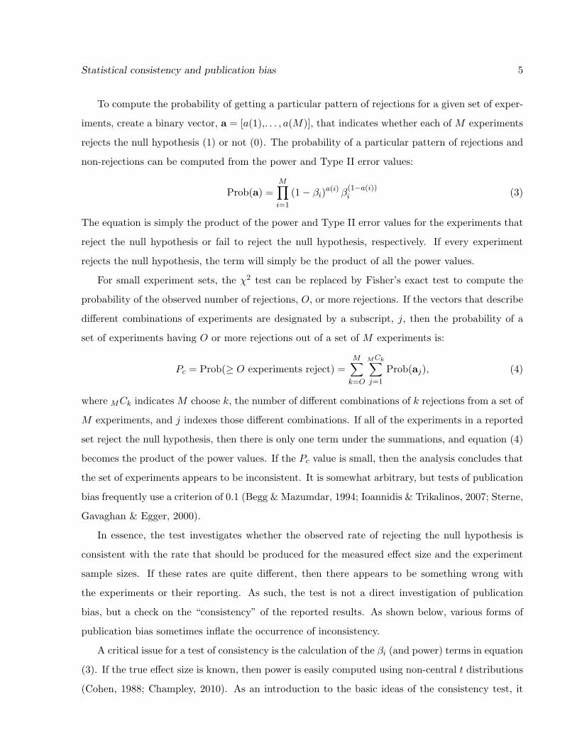
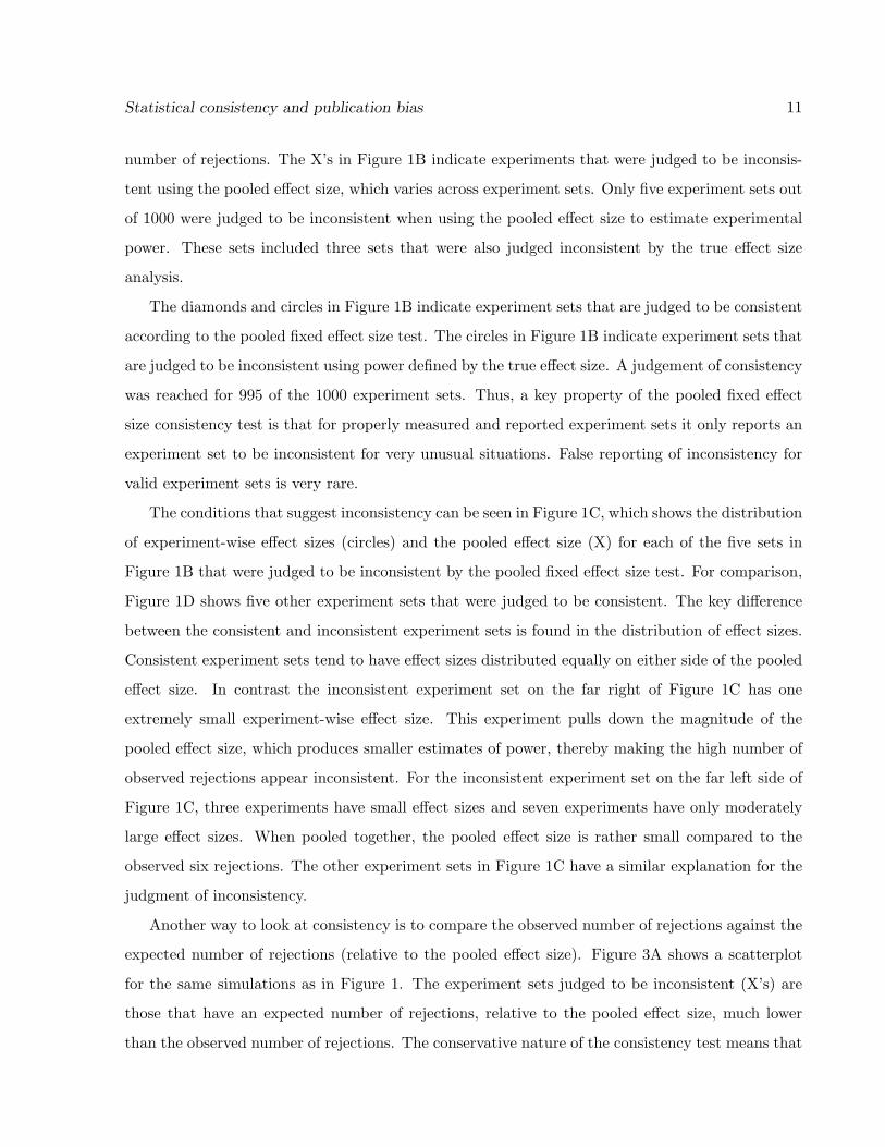
Another way to look at consistency is to compare the observed number of rejections against the
expected number of rejections (relative to the pooled e↵ect size). Figure 3A shows a scatterplot
for the same simulations as in Figure 1. The experiment sets judged to be inconsistent (X’s) are
those that have an expected number of rejections, relative to the pooled e↵ect size, much lower
than the observed number of rejections. The conservative nature of the consistency test means that
Statistical consistency and publication bias 12
0 2 4 6 8 10Observed number of rejections
0
2
4
6
8
10
Expe
cted
num
ber o
f rej
ectio
ns
ConsistentTrue ES inconsistentPooled ES inconsistent
0 2 4 6 8 10Observed number of rejections
0
2
4
6
8
10
Expe
cted
num
ber o
f rej
ectio
ns
ConsistentTrue ES inconsistentPooled ES inconsistent
B Biased experiment setsA Unbiased experiment sets
Figure 3: A comparison of the expected number of rejections (the sum of the power values within an
experimental set) against the observed number of rejections indicates how inconsistent experiment
sets (X’s) are unusual when using the power computed from the pooled fixed e↵ect size. The circles
correspond to inconsistent sets when power is defined relative to the true e↵ect size. The cases
in A correspond to the unbiased simulations in Figure 1, while the cases in B correspond to the
simulations in Figure 2 where a file-drawer bias suppressed experiments that did not reject the null
hypothesis.
when experiments are reported fully and run properly, it is quite rare to reach a conclusion of an
experiment set appearing to be inconsistent.
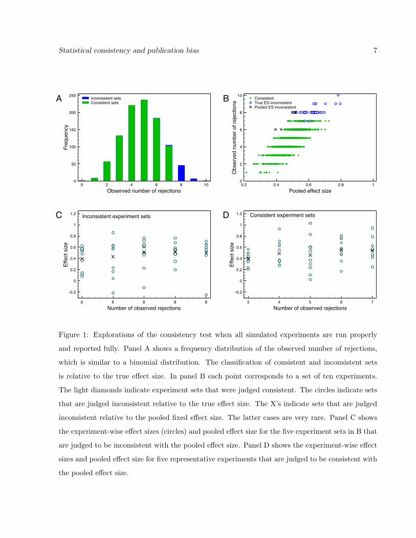
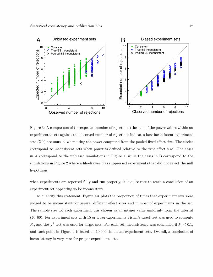
To quantify this statement, Figure 4A plots the proportion of times that experiment sets were
judged to be inconsistent for several di↵erent e↵ect sizes and number of experiments in the set.
The sample size for each experiment was chosen as an integer value uniformly from the interval
(40, 60). For experiment sets with 15 or fewer experiments Fisher’s exact test was used to compute
Pc, and the �2 test was used for larger sets. For each set, inconsistency was concluded if Pc 0.1,
and each point in Figure 4 is based on 10,000 simulated experiment sets. Overall, a conclusion of
inconsistency is very rare for proper experiment sets.

Statistical consistency and publication bias 13
1 10 100Experiment set size
0
0.2
0.4
0.6
0.8
1
Prop
ortio
n of
set
s ju
dged
inco
nsis
tent
0.10.20.30.40.50.60.70.80.91.0
1 10 100Experiment set size
0
0.2
0.4
0.6
0.8
1
Prop
ortio
n of
set
s ju
dged
inco
nsis
tent
0.10.20.30.40.50.60.70.80.91.0
1 10 100Reported experiment set size
0
0.2
0.4
0.6
0.8
1
Prop
ortio
n of
set
s ju
dged
inco
nsis
tent
0.10.20.30.40.50.60.70.80.91.0
A
B
C
True effect size
True effect size
True effect size
Figure 4: Each plot shows the proportion of simulated experiment sets where the pooled fixed
e↵ect size consistency test concludes that the set is inconsistent. Separate curves are for di↵erent
true e↵ect sizes. Panel A demonstrates that the test rarely concludes inconsistency when the
experiments are run properly and reported fully. The proportions are well below the criterion
value of 0.1. Panel B demonstrates that when a file-drawer bias is used to suppress null/negative
experimental findings the consistency test is more likely to report inconsistency for intermediate
e↵ect sizes and larger numbers of experiments in a set. Panel C re-plots the data from B relative
to the reported number of experiments in a set (not including the suppressed findings). The test
is more likely to report bias for reported experiment sets with small true e↵ect sizes.
Statistical consistency and publication bias 14
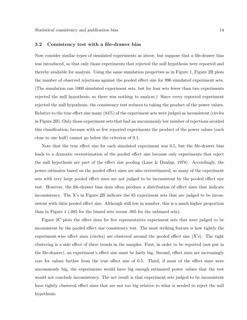
3.2 Consistency test with a file-drawer bias
Now consider similar types of simulated experiments as above, but suppose that a file-drawer bias
was introduced, so that only those experiments that rejected the null hypothesis were reported and
thereby available for analysis. Using the same simulation properties as in Figure 1, Figure 2B plots
the number of observed rejections against the pooled e↵ect size for 996 simulated experiment sets.
(The simulation ran 1000 simulated experiment sets, but for four sets fewer than two experiments
rejected the null hypothesis, so there was nothing to analyze.) Since every reported experiment
rejected the null hypothesis, the consistency test reduces to taking the product of the power values.
Relative to the true e↵ect size many (84%) of the experiment sets were judged as inconsistent (circles
in Figure 2B). Only those experiment sets that had an uncommonly low number of rejections avoided
this classification, because with so few reported experiments the product of the power values (each
close to one half) cannot go below the criterion of 0.1.
Note that the true e↵ect size for each simulated experiment was 0.5, but the file-drawer bias
leads to a dramatic overestimation of the pooled e↵ect size because only experiments that reject
the null hypothesis are part of the e↵ect size pooling (Lane & Dunlap, 1978). Accordingly, the
power estimates based on the pooled e↵ect sizes are also overestimated, so many of the experiment
sets with very large pooled e↵ect sizes are not judged to be inconsistent by the pooled e↵ect size
test. However, the file-drawer bias does often produce a distribution of e↵ect sizes that indicate
inconsistency. The X’s in Figure 2B indicate the 85 experiment sets that are judged to be incon-
sistent with their pooled e↵ect size. Although still low in number, this is a much higher proportion
than in Figure 1 (.085 for the biased sets versus .005 for the unbiased sets).
Figure 2C plots the e↵ect sizes for five representative experiment sets that were judged to be
inconsistent by the pooled e↵ect size consistency test. The most striking feature is how tightly the
experiment-wise e↵ect sizes (circles) are clustered around the pooled e↵ect size (X’s). The tight
clustering is a side e↵ect of three trends in the samples. First, in order to be reported (not put in
the file-drawer), an experiment’s e↵ect size must be fairly big. Second, e↵ect sizes are increasingly
rare for values further from the true e↵ect size of 0.5. Third, if most of the e↵ect sizes were
uncommonly big, the experiments would have big enough estimated power values that the test
would not conclude inconsistency. The net result is that experiment sets judged to be inconsistent
have tightly clustered e↵ect sizes that are not too big relative to what is needed to reject the null
hypothesis.
Statistical consistency and publication bias 15
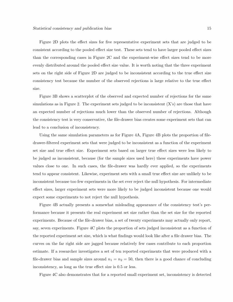
Figure 2D plots the e↵ect sizes for five representative experiment sets that are judged to be
consistent according to the pooled e↵ect size test. These sets tend to have larger pooled e↵ect sizes
than the corresponding cases in Figure 2C and the experiment-wise e↵ect sizes tend to be more
evenly distributed around the pooled e↵ect size value. It is worth noting that the three experiment
sets on the right side of Figure 2D are judged to be inconsistent according to the true e↵ect size
consistency test because the number of the observed rejections is large relative to the true e↵ect
size.
Figure 3B shows a scatterplot of the observed and expected number of rejections for the same
simulations as in Figure 2. The experiment sets judged to be inconsistent (X’s) are those that have
an expected number of rejections much lower than the observed number of rejections. Although
the consistency test is very conservative, the file-drawer bias creates some experiment sets that can
lead to a conclusion of inconsistency.
Using the same simulation parameters as for Figure 4A, Figure 4B plots the proportion of file-
drawer-filtered experiment sets that were judged to be inconsistent as a function of the experiment
set size and true e↵ect size. Experiment sets based on larger true e↵ect sizes were less likely to
be judged as inconsistent, because (for the sample sizes used here) these experiments have power
values close to one. In such cases, the file-drawer was hardly ever applied, so the experiments
tend to appear consistent. Likewise, experiment sets with a small true e↵ect size are unlikely to be
inconsistent because too few experiments in the set ever reject the null hypothesis. For intermediate
e↵ect sizes, larger experiment sets were more likely to be judged inconsistent because one would
expect some experiments to not reject the null hypothesis.
Figure 4B actually presents a somewhat misleading appearance of the consistency test’s per-
formance because it presents the real experiment set size rather than the set size for the reported
experiments. Because of the file-drawer bias, a set of twenty experiments may actually only report,
say, seven experiments. Figure 4C plots the proportion of sets judged inconsistent as a function of
the reported experiment set size, which is what findings would look like after a file drawer bias. The
curves on the far right side are jagged because relatively few cases contribute to each proportion
estimate. If a researcher investigates a set of ten reported experiments that were produced with a
file-drawer bias and sample sizes around n1 = n2 = 50, then there is a good chance of concluding
inconsistency, as long as the true e↵ect size is 0.5 or less.
Figure 4C also demonstrates that for a reported small experiment set, inconsistency is detected
Statistical consistency and publication bias 16
more often when the true e↵ect size is small. This is because with a small true e↵ect size, it is
ever more rare for an experiment to have a large enough e↵ect size to reject the null hypothesis.
Thus, those experiments that do reject the null hypothesis tend to just barely do so. For such
experiments, the resulting power values tend to be close to one half, so even four such experiments
will lead to a conclusion of inconsistency.
Overall, the pooled e↵ect size version of the consistency test is extremely conservative. It rarely
concludes inconsistency when a set of experiments are run properly and fully reported. A negative
side e↵ect of such conservatism is that it also misses many situations with a strong file-drawer bias.
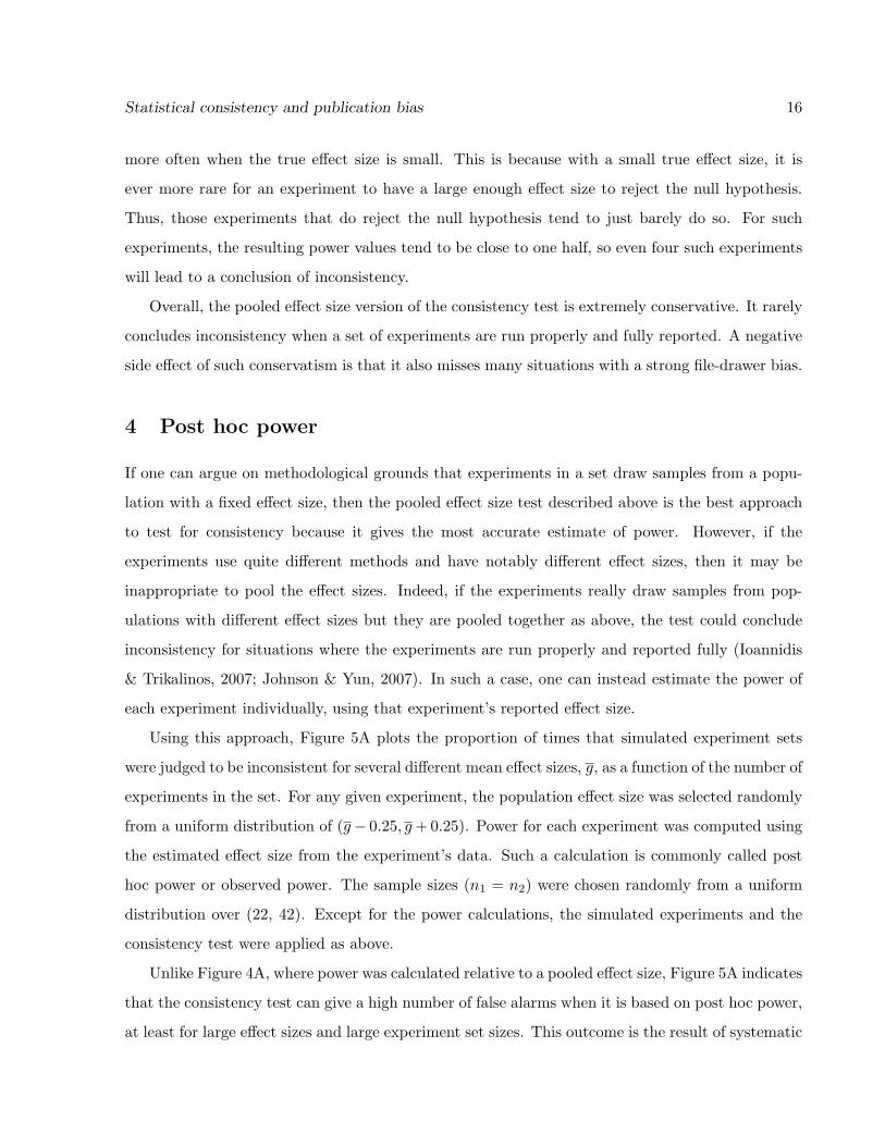
4 Post hoc power
If one can argue on methodological grounds that experiments in a set draw samples from a popu-
lation with a fixed e↵ect size, then the pooled e↵ect size test described above is the best approach
to test for consistency because it gives the most accurate estimate of power. However, if the
experiments use quite di↵erent methods and have notably di↵erent e↵ect sizes, then it may be
inappropriate to pool the e↵ect sizes. Indeed, if the experiments really draw samples from pop-
ulations with di↵erent e↵ect sizes but they are pooled together as above, the test could conclude
inconsistency for situations where the experiments are run properly and reported fully (Ioannidis
& Trikalinos, 2007; Johnson & Yun, 2007). In such a case, one can instead estimate the power of
each experiment individually, using that experiment’s reported e↵ect size.
Using this approach, Figure 5A plots the proportion of times that simulated experiment sets
were judged to be inconsistent for several di↵erent mean e↵ect sizes, g, as a function of the number of
experiments in the set. For any given experiment, the population e↵ect size was selected randomly
from a uniform distribution of (g� 0.25, g + 0.25). Power for each experiment was computed using
the estimated e↵ect size from the experiment’s data. Such a calculation is commonly called post
hoc power or observed power. The sample sizes (n1 = n2) were chosen randomly from a uniform
distribution over (22, 42). Except for the power calculations, the simulated experiments and the
consistency test were applied as above.
Unlike Figure 4A, where power was calculated relative to a pooled e↵ect size, Figure 5A indicates
that the consistency test can give a high number of false alarms when it is based on post hoc power,
at least for large e↵ect sizes and large experiment set sizes. This outcome is the result of systematic
Statistical consistency and publication bias 17
1 10 100Experiment set size
0
0.2
0.4
0.6
0.8
1
Prop
ortio
n of
set
s ju
dged
inco
nsis
tent
0.10.20.30.40.50.60.70.80.91.0
1 10 100Experiment set size
0
0.2
0.4
0.6
0.8
1
Prop
ortio
n of
set
s ju
dged
inco
nsis
tent
0.10.20.30.40.50.60.70.80.91.0
1 10 100Experiment set size
0
0.2
0.4
0.6
0.8
1
Prop
ortio
n of
set
s ju
dged
inco
nsis
tent
0.10.20.30.40.50.60.70.80.91.0
A
B
C
Mean true effect size
Mean true effect size
Mean true effect size
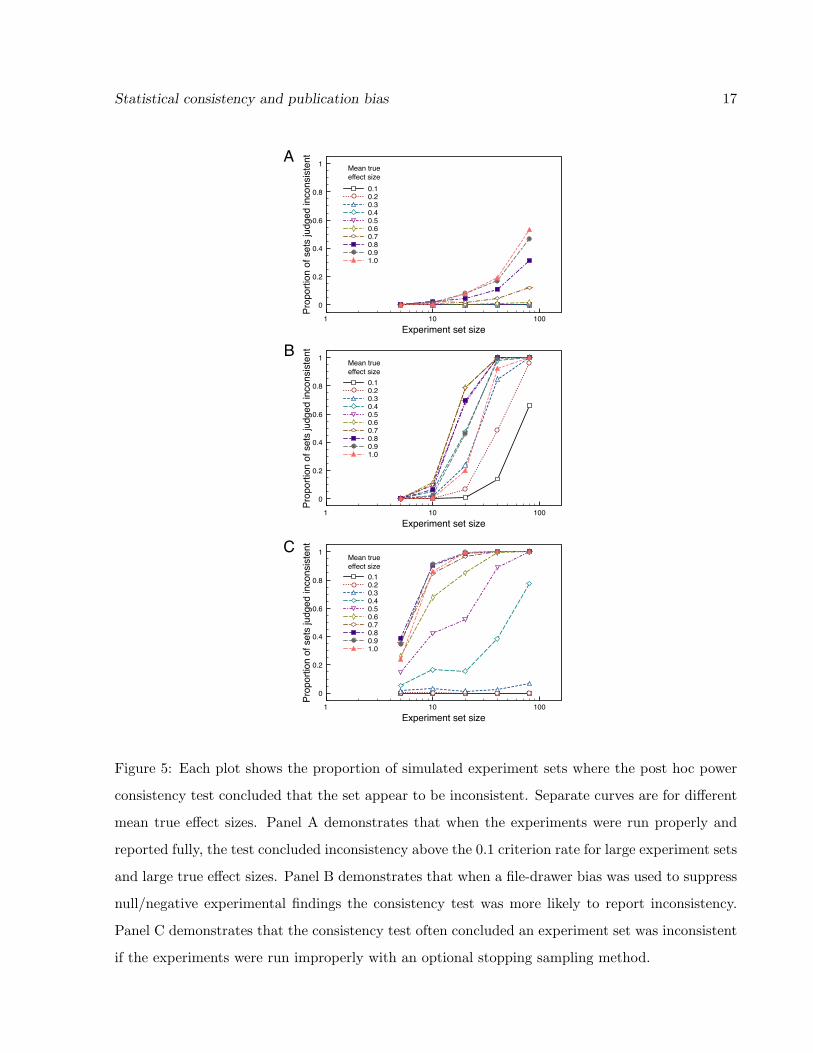
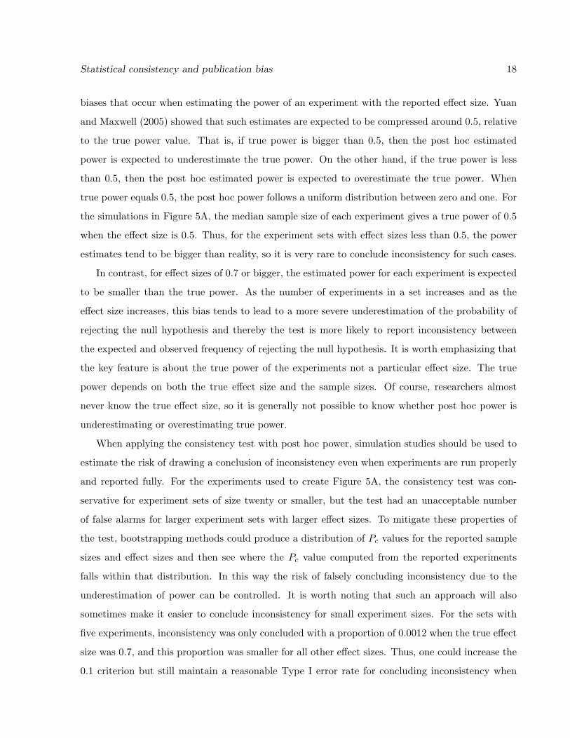
Figure 5: Each plot shows the proportion of simulated experiment sets where the post hoc power
consistency test concluded that the set appear to be inconsistent. Separate curves are for di↵erent
mean true e↵ect sizes. Panel A demonstrates that when the experiments were run properly and
reported fully, the test concluded inconsistency above the 0.1 criterion rate for large experiment sets
and large true e↵ect sizes. Panel B demonstrates that when a file-drawer bias was used to suppress
null/negative experimental findings the consistency test was more likely to report inconsistency.
Panel C demonstrates that the consistency test often concluded an experiment set was inconsistent
if the experiments were run improperly with an optional stopping sampling method.
Statistical consistency and publication bias 18
biases that occur when estimating the power of an experiment with the reported e↵ect size. Yuan
and Maxwell (2005) showed that such estimates are expected to be compressed around 0.5, relative
to the true power value. That is, if true power is bigger than 0.5, then the post hoc estimated
power is expected to underestimate the true power. On the other hand, if the true power is less
than 0.5, then the post hoc estimated power is expected to overestimate the true power. When
true power equals 0.5, the post hoc power follows a uniform distribution between zero and one. For
the simulations in Figure 5A, the median sample size of each experiment gives a true power of 0.5
when the e↵ect size is 0.5. Thus, for the experiment sets with e↵ect sizes less than 0.5, the power
estimates tend to be bigger than reality, so it is very rare to conclude inconsistency for such cases.
In contrast, for e↵ect sizes of 0.7 or bigger, the estimated power for each experiment is expected
to be smaller than the true power. As the number of experiments in a set increases and as the
e↵ect size increases, this bias tends to lead to a more severe underestimation of the probability of
rejecting the null hypothesis and thereby the test is more likely to report inconsistency between
the expected and observed frequency of rejecting the null hypothesis. It is worth emphasizing that
the key feature is about the true power of the experiments not a particular e↵ect size. The true
power depends on both the true e↵ect size and the sample sizes. Of course, researchers almost
never know the true e↵ect size, so it is generally not possible to know whether post hoc power is
underestimating or overestimating true power.
When applying the consistency test with post hoc power, simulation studies should be used to
estimate the risk of drawing a conclusion of inconsistency even when experiments are run properly
and reported fully. For the experiments used to create Figure 5A, the consistency test was con-
servative for experiment sets of size twenty or smaller, but the test had an unacceptable number
of false alarms for larger experiment sets with larger e↵ect sizes. To mitigate these properties of
the test, bootstrapping methods could produce a distribution of Pc values for the reported sample
sizes and e↵ect sizes and then see where the Pc value computed from the reported experiments
falls within that distribution. In this way the risk of falsely concluding inconsistency due to the
underestimation of power can be controlled. It is worth noting that such an approach will also
sometimes make it easier to conclude inconsistency for small experiment sizes. For the sets with
five experiments, inconsistency was only concluded with a proportion of 0.0012 when the true e↵ect
size was 0.7, and this proportion was smaller for all other e↵ect sizes. Thus, one could increase the
0.1 criterion but still maintain a reasonable Type I error rate for concluding inconsistency when
Statistical consistency and publication bias 19
experiments are run properly and reported fully.
4.1 Consistency test with biased experiment sets
Figure 5B shows the behavior of the post hoc power consistency test when an experiment set
was subjected to an extreme file-drawer bias, where only those experiments that reject the null
hypothesis were reported. The results are similar to those in Figure 4B, except that the post hoc
power analysis frequently indicates inconsistency for experiment sets with large e↵ect sizes. Again,
this is due to the underestimation of true power for experiments with large true power values.
Just as for Figure 4B, it is important to remember that what is described in Figure 5B is the true
number of experiments, not the reported number of experiments.
Figure 5C describes the behavior of the consistency test for another type of bias: optional
stopping. The normal interpretation of the p value in a hypothesis test (as the probability of an
observed, or more extreme, outcome if the null hypothesis is true), is only valid for a fixed sample
size (which is used to define the sampling distribution). If the sample size is not fixed, then the
traditional sampling distribution is inappropriate and the analysis is invalid (Wagenmakers, 2007;
Kruschke, 2010a). Unfortunately, some researchers seem to engage in sampling practices that lead
to invalid hypothesis tests (John et al., 2012). In an optional stopping approach, a researcher may
gather an initial set of data and check the statistical analysis. If the null hypothesis is rejected, the
experiment is stopped and reported, but if the null hypothesis is not rejected additional data points
are collected and combined with the old data. The statistical analysis is repeated and the same
criterion used until either the null hypothesis is rejected or the researcher stops the experiment.
Such optional stopping dramatically inflates the rate of rejecting the null hypothesis. In particular,
it increases the Type I error rate, and if a researcher is willing to add enough samples, the probability
of rejecting the null hypothesis approaches one (Anscombe, 1954).
Optional stopping creates inconsistent data sets in two ways. First, for experiments that reject
the null hypothesis, the post hoc power of an experiment based on optional stopping is often just
a bit more than one half because the experiment stops once the null hypothesis has been rejected.
This outcome is true regardless of the details of the optional stopping method. The only exceptions
are when the starting sample size and true e↵ect size are so large that there is overwhelming evidence
against the null hypothesis without ever adding additional data points. Second, for experiments
that reject the null hypothesis, an experiment will sometimes stop with an estimated e↵ect size
Statistical consistency and publication bias 20
smaller than the true e↵ect size because even the small e↵ect allows for rejecting the null hypothesis.
Thus, experiments based on optional stopping can simultaneously underestimate the magnitude of
true e↵ects and exaggerate the rejection rate of experiments (Ioannidis, 2008; Francis, 2012g).
Simulated experiments were created with optional stopping. Each experiment started with a
random sample of n1 = n2 = 15 and added one additional data point until rejecting the null
hypothesis or reaching a maximum sample size of 32. As Figure 5C shows, the consistency test
was quite sensitive to some experiment sets created by optional stopping (there is no file-drawer
for these experiment sets). Even for a set of just five experiments, the proportion of sets judged
inconsistent nears 40% for all but the smallest e↵ect sizes. This is because the experiments that
reject the null hypothesis tend to just barely do so. Each experiment stopped gathering data before
su�ciently strong evidence for the alternative hypothesis was gathered. In contrast, if fixed sample
sizes were used for powerful experiments, one would expect to often find much stronger evidence
against the null hypothesis (Cumming, 2008).
5 Using a random e↵ects model
It is common in meta-analyses to suppose that experiments in a set draw their samples from slightly
di↵erent populations that are related by a distribution of e↵ect sizes. A common approach is to
treat the distribution as a normal distribution with an estimated mean and variance (Borenstein,
Hedges, Higgins & Rothstein, 2009). To develop a random e↵ects model, first use the gi and wi
terms from equations (7) and (10) to compute
Q =MX
i=1
wig2i �
⇣PMi=1 wigi
⌘2
PMi=1 wi
(13)
and
C =MX
i=1
wi �PM
i=1 w2iPM
i=1 wi
(14)
to produce an estimate of the variance between experiment e↵ect sizes
T 2 = maxQ� (M � 1)
C, 0�. (15)
Define new weights for the e↵ect size pooling by using both the variance for an experiment and the
between experiment variance
w⇤i =1
vgi + T 2. (16)

Statistical consistency and publication bias 21
The estimated mean of the e↵ect size distribution is then
g⇤ =PM
i=1 w⇤i giPMi=1 w⇤i
. (17)
The power of experiments under a random e↵ects model should consider the variability that
would be introduced by variations in the sampled e↵ect sizes. This can be done by computing
expected power (Gillett, 1994), which takes into account the uncertainty in the e↵ect size that will
vary across experiments. The expected power for experiment i would be computed as1
E [Poweri] =Z 1
�1[1� �(g, ni1, ni2)]N (g; g⇤, T )dg, (18)
which includes the sample sizes ni1 and ni2 that were used in the original experiment. N (g; g⇤, T ) is
the probability density function for an e↵ect size, g. This normal distribution has a mean g⇤ and a
standard deviation T that is estimated from the experiments. One could also consider a distribution
of sample sizes, but this supposes knowledge about the intentions of the experimenter. One could
also incorporate the uncertainty about g⇤ and T with their probability density distributions, but
there may be diminishing returns relative to the complexity of the computations.
Similar to post hoc power, expected power tends to underestimate true power when the true
power is bigger than one half and overestimates true power when the true power is smaller than
one half (Yuan & Maxwell, 2005). More uncertainty about the e↵ect size tends to enhance these
mis-estimations. Nevertheless, given the information available, expected power is the best estimate
of an experiment’s power in a random e↵ects model. Expected power could also be used for the
fixed e↵ect case above, but it tends to not make much di↵erence because the pooled e↵ect size
typically has a small variance. Using expected power for the post hoc calculations would make the
test less likely to conclude inconsistency for low power experiment sets and more likely for high
power experiment sets.
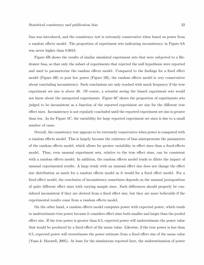
Figure 6A plots the proportion of times that experiment sets were judged to be inconsistent for
several di↵erent mean e↵ect sizes, g, as a function of the number of experiments in the set. For
any given experiment, the population e↵ect size was selected randomly from a normal distribution
of N (g, 0.5). The sample sizes were chosen randomly from a uniform distribution over (22, 42).
Other aspects of the simulations were as described above. For the experiments in Figure 6A, no1Due to a quirk of numerical integration in the R programming language (R Development Core Team, 2011),
having T 2 < 0.0001 produced an expected power of zero. To avoid this problem, when T 2 < 0.0001, power was
computed with the point estimate of g⇤. For the cases reported here, these two calculations are almost identical.
Statistical consistency and publication bias 22
bias was introduced, and the consistency test is extremely conservative when based on power from
a random e↵ects model. The proportion of experiment sets indicating inconsistency in Figure 6A
was never higher than 0.0018.
Figure 6B shows the results of similar simulated experiment sets that were subjected to a file-
drawer bias, so that only the subset of experiments that rejected the null hypothesis were reported
and used to parameterize the random e↵ects model. Compared to the findings for a fixed e↵ect
model (Figure 4B) or post hoc power (Figure 5B), the random e↵ects model is very conservative
about concluding inconsistency. Such conclusions are only reached with much frequency if the true
experiment set size is above 40. Of course, a scientist seeing the biased experiment sets would
not know about the unreported experiments. Figure 6C shows the proportion of experiments sets
judged to be inconsistent as a function of the reported experiment set size for the di↵erent true
e↵ect sizes. Inconsistency is not regularly concluded until the reported experiment set size is greater
than ten. As for Figure 5C, the variability for large reported experiment set sizes is due to a small
number of cases.
Overall, the consistency test appears to be extremely conservative when power is computed with
a random e↵ects model. This is largely because the existence of bias misrepresents the parameters
of the random e↵ects model, which allows for greater variability in e↵ect sizes than a fixed-e↵ects
model. Thus, even unusual experiment sets, relative to the true e↵ect sizes, can be consistent
with a random e↵ects model. In addition, the random e↵ects model tends to dilute the impact of
unusual experimental results. A large study with an unusual e↵ect size does not change the e↵ect
size distribution as much for a random e↵ects model as it would for a fixed e↵ect model. For a
fixed e↵ect model, the conclusion of inconsistency sometimes depends on the unusual juxtaposition
of quite di↵erent e↵ect sizes with varying sample sizes. Such di↵erences should properly be con-
sidered inconsistent if they are derived from a fixed e↵ect size, but they are more believable if the
experimental results come from a random e↵ects model.
On the other hand, a random e↵ects model computes power with expected power, which tends
to underestimate true power because it considers e↵ect sizes both smaller and larger than the pooled
e↵ect size. If the true power is greater than 0.5, expected power will underestimate the power value
that would be produced by a fixed e↵ect of the mean value. Likewise, if the true power is less than
0.5, expected power will overestimate the power estimate from a fixed e↵ect size of the mean value
(Yuan & Maxwell, 2005). At least for the simulations reported here, the underestimation of power

Statistical consistency and publication bias 23
1 10 100Reported experiment set size
0
0.2
0.4
0.6
0.8
1
Prop
ortio
n of
set
s ju
dged
inco
nsis
tent
0.10.20.30.40.50.60.70.80.91.0
1 10 100Experiment set size
0
0.2
0.4
0.6
0.8
1
Prop
ortio
n of
set
s ju
dged
inco
nsis
tent
0.10.20.30.40.50.60.70.80.91.0
1 10 100Reported experiment set size
0
0.2
0.4
0.6
0.8
1
Prop
ortio
n of
set
s ju
dged
inco
nsis
tent
0.10.20.30.40.50.60.70.80.91.0
A
B
C
Mean true effect size
Mean true effect size
Mean true effect size
Figure 6: Each plot shows the proportion of simulated experiment sets where the random e↵ect
size consistency test concluded that the set appears to be inconsistent. Separate curves are for
di↵erent mean true e↵ect sizes. Panel A demonstrates that when the experiments are run properly
and reported fully, the test rarely concludes inconsistency. Panel B demonstrates that when a
file-drawer bias was used to suppress null/negative experimental findings the consistency test was
more likely to report inconsistency for bigger e↵ect sizes and larger experiment set sizes. Panel C
re-plots the data from B relative to the reported number of experiments in a set (not including the
suppressed null findings). The test is more likely to report bias for small e↵ect sizes.

Statistical consistency and publication bias 24
does not frequently lead to a false conclusion of inconsistency, although it might in other situations.
6 Putting the consistency test to practice
As one example of applying the consistency test, consider a report by Topolinski and Sparen-
berg (2012), which concluded that individuals instigating or observing clockwise movements are
more accepting of novelty. They argued that the conceptual representation of time moving in a
clockwise direction produced a psychological state consistent with temporal progression and thus
novelty. For example, in their fourth experiment, participants were asked to choose jellybeans from
a rotating tray that was rigged to only spin either clockwise or counterclockwise. Compared to
participants with a counterclockwise rotating tray, participants in the clockwise condition selected
more unconventional flavors of jellybeans. The di↵erence was statistically significant, and three
other experiments reached a similar conclusion by having participants observe a rotating shape, or
physically rotate a tube or crank. In every case, with di↵erent tasks and measures, participants
in the clockwise condition behaved in a way that indicated a preference for novelty. The findings
across experiments led the authors to conclude that the experimental results provided strong evi-
dence that abstract sensorimotor symbols activated temporal representations and thereby a novelty
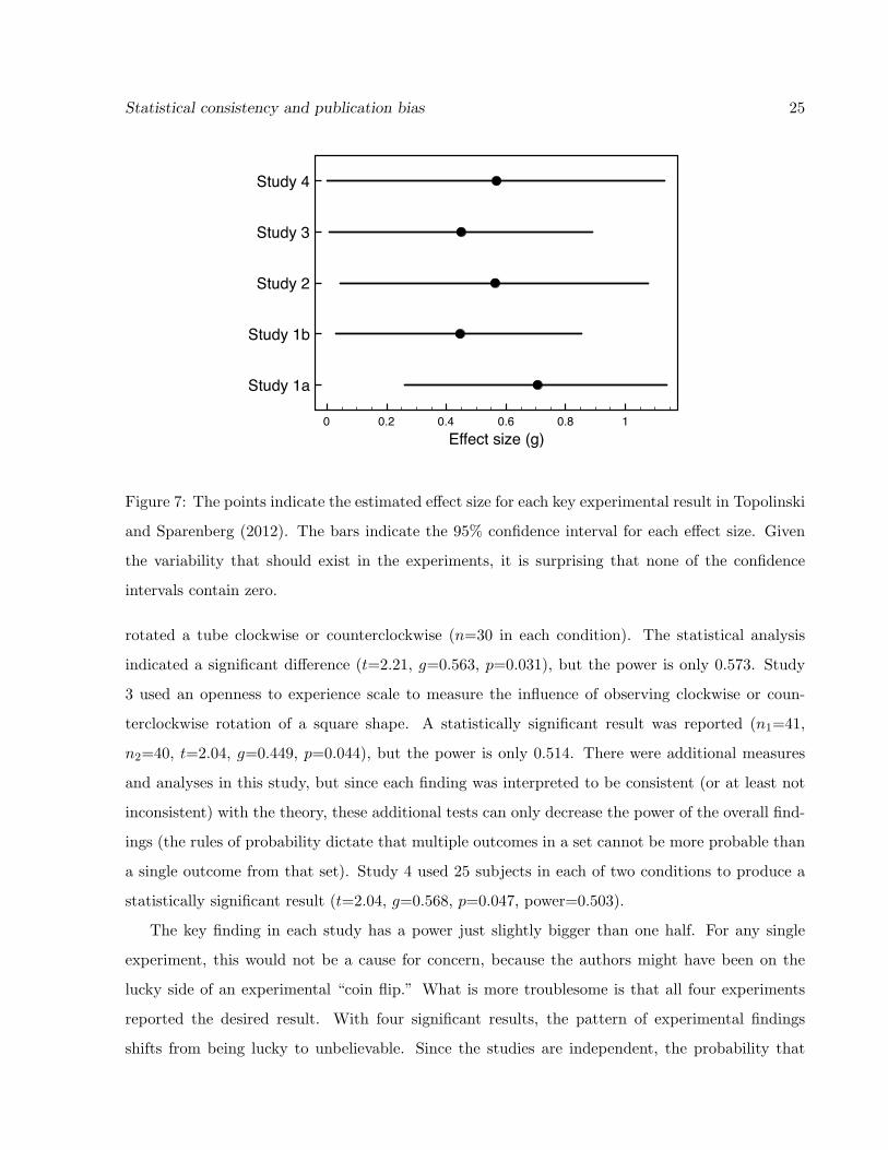
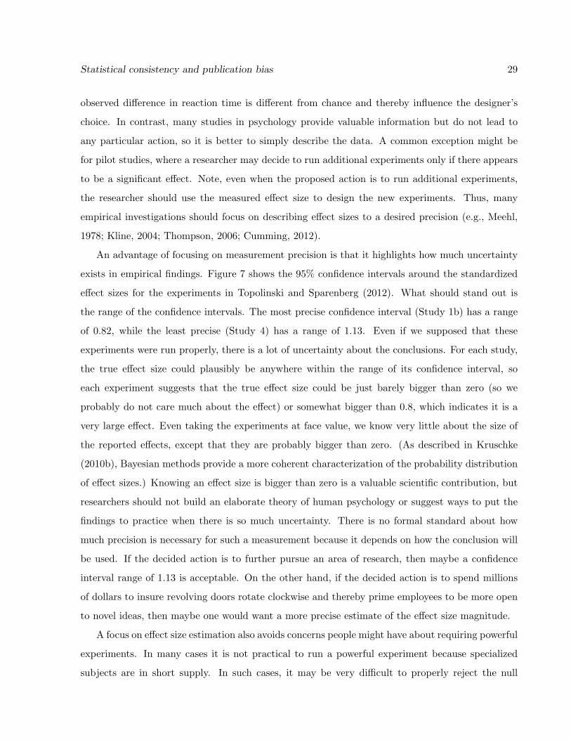
preference. Figure 7 plots the estimated e↵ect size for each experiment and its 95% confidence in-
terval (Kelley, 2007). Study 1a measures a control condition, but the other experiments measure
similar variables. It is clear that the observed di↵erences in e↵ect sizes for studies 1b–4 are small
compared to the range of the confidence intervals. One could pool the e↵ect sizes from studies
1b–4, but given the methodological di↵erences across the experiments, a post hoc power analysis
seems more appropriate. In practice, when the sample sizes and e↵ect sizes are similar, it hardly
matters which approach is used.
Study 1 concluded evidence for the theory by contrasting the statistical outcome from two in-
dependent groups who rotated a crank. A control (rotate counterclockwise) group showed a strong
mere exposure e↵ect to a set of stimuli (n=25, t=3.64, g=0.705, p=0.001, power=0.922), while
an experimental (rotate clockwise) group showed a modest preference for novelty (n=25, t=2.30,
g=0.445, p=.030, power=0.571). The estimated probability of both groups showing the observed
pattern in experiments like these is the product of the powers, which is 0.526. The evidence from
Study 2 was based on a statistical test of reported openness to experience for participants who
Statistical consistency and publication bias 25
0 0.2 0.4 0.6 0.8 1Effect size (g)
Study 1a
Study 1b
Study 2
Study 3
Study 4
Figure 7: The points indicate the estimated e↵ect size for each key experimental result in Topolinski
and Sparenberg (2012). The bars indicate the 95% confidence interval for each e↵ect size. Given
the variability that should exist in the experiments, it is surprising that none of the confidence
intervals contain zero.
rotated a tube clockwise or counterclockwise (n=30 in each condition). The statistical analysis
indicated a significant di↵erence (t=2.21, g=0.563, p=0.031), but the power is only 0.573. Study
3 used an openness to experience scale to measure the influence of observing clockwise or coun-
terclockwise rotation of a square shape. A statistically significant result was reported (n1=41,
n2=40, t=2.04, g=0.449, p=0.044), but the power is only 0.514. There were additional measures
and analyses in this study, but since each finding was interpreted to be consistent (or at least not
inconsistent) with the theory, these additional tests can only decrease the power of the overall find-
ings (the rules of probability dictate that multiple outcomes in a set cannot be more probable than
a single outcome from that set). Study 4 used 25 subjects in each of two conditions to produce a
statistically significant result (t=2.04, g=0.568, p=0.047, power=0.503).
The key finding in each study has a power just slightly bigger than one half. For any single
experiment, this would not be a cause for concern, because the authors might have been on the
lucky side of an experimental “coin flip.” What is more troublesome is that all four experiments
reported the desired result. With four significant results, the pattern of experimental findings
shifts from being lucky to unbelievable. Since the studies are independent, the probability that

Statistical consistency and publication bias 26
four studies like those reported by Topolinski and Sparenberg (2012) would all produce outcomes
that supported the theory is the product of the power values: 0.573 ⇥ 0.526 ⇥ 0.514 ⇥ 0.503 =
0.078. If the studies were run properly and reported fully and if the theory had e↵ects equivalent
to what was reported by the experiments, then this is the probability that all four studies would
produce the reported pattern of results. The probability of the experiment set is low enough to
conclude that the reported results appear inconsistent, which suggests that either the experiments
were not fully reported or were not run properly.
What are the odds that the test would incorrectly conclude inconsistency if experiments like
these were truly run properly and reported fully? The far left side of the curves in Figure 5A
suggests that such probabilities are very low, but the experiments in Topolinski and Sparenberg
(2012) were with di↵erent samples sizes and estimated e↵ect sizes. New simulations can make
an estimate for the types of experiments reported by Topolinski and Sparenberg (2012). Ten
thousand simulated experiment sets with the g values and samples sizes reported by Topolinski
and Sparenberg (2012) were tested for inconsistency using the post hoc power version of the test.
Each simulated experiment followed the requirements for hypothesis testing (samples drawn from
a normal distribution, homogeneity of variance) and every experimental outcome was reported,
regardless of the hypothesis test conclusion. Under such a situation, the expected number of
significant findings is the sum of the power values, which is 2.975. Indeed, the mean number of
rejections across the five simulated experiments was 3.081. Only 17 out of 10,000 such simulated
experiment sets concluded inconsistency. The proportion of simulated experiment sets with a
consistency probability value Pc smaller than what was observed for the Topolinski and Sparenberg
(2012) set was 0.0012. The 10th percentile for the Pc values was 0.342, so the 0.1 criterion was
extremely conservative for these kinds of experiments.
The consistency test cannot discriminate between di↵erent kinds of bias that might lead to
the conclusion of inconsistency. It could be that Topolinski and Sparenberg (2012) suppressed
experiments or measures of variables that did not show results consistent with their theory (Phillips,
2004). They may have used inappropriate research practices (Simmons et al., 2011; John et al.,
2012) that inflated the rate of rejecting the null hypothesis. An optional stopping approach would
explain how Topolinski and Sparenberg (2012) almost always used sample sizes that just barely
rejected the null hypothesis. Regardless of how the results were generated, scientists should be
skeptical of their validity because, without some kind of inappropriate bias, they appear to be
Statistical consistency and publication bias 27
inconsistent.
Not believing the reported results does not require an accusation of intentional misconduct
by Topolinski and Sparenberg (2012). Very likely bias crept into their experiment set without
their awareness. They may have made choices in data collection, analysis, and interpretation that
lead to the biased results but did not realize that their choices made their findings inconsistent.
Moreover, they may have been pressured by reviewers to engage in these practices to make the
story “cleaner” or “stronger.” A common request from reviewers is to run more subjects to push
an almost significant finding past the threshold to reject the null hypothesis. Such actions sound
like good scientific practice to reach a definitive conclusion, but they actually violate the tenets of
hypothesis testing (Kruschke, 2010a). Not believing the reported results also does not necessarily
require disbelief in the proposed theory. The logical interpretation of a biased set of findings is that
they do not provide proper evidence one way or another. Of course, the burden of proof is for the
proponents of the theory, and only new unbiased experiments can provide such evidence.
7 How can experimenters ensure they produce consistent sets of
experiments?
Although there have been several high profile reports of fraud in psychology (Enserink, 2011; Yong,
2012b), such cases are probably rare. However, it appears to be very common for researchers to
engage in what are called “questionable research practices” (John et al., 2012) such as optional stop-
ping, multiple testing, subject dropping, and hypothesizing after the results are known (HARKing;
Kerr, 1998). These types of activities can lead to inconsistent data sets because these practices
tend to stop as soon as a statistically significant result is found. The term “questionable” is really
a misnomer, because these activities actually render scientific investigations “invalid.” The term
questionable only reflects the (mis)understanding researchers have about the impact of these meth-
ods on the validity of experimental results. Many researchers are unaware that such methods can
have an enormous impact on the integrity of their research findings (e.g., Simmons et al., 2011).
In a sense, it is easy to produce a consistent set of experiments: run the experiments properly
and report them fully. If researchers stick to the principles of hypothesis testing (e.g., fixed sample
size) and analyze the data appropriately (e.g., with the tests planned out in advance), then a full
report of the findings will almost always be consistent and valid. In practice, it is often di�cult
Statistical consistency and publication bias 28
to follow this prescription. In many cases data collection is not based on a fixed sample size but
on the availability of participants over a certain time frame (Kruschke, 2010a). After data has
been gathered it is very tempting to explore patterns in the data regardless of the original plans,
and it seems almost unethical to waste carefully gathered data by not squeezing out all possible
information. An article where only a small subset of the experiments finds a significant result is
likely unpublishable in academic journals. Even for a small number of null findings, reviewers often
insist on an explanation for the apparent discrepancies, which tends to promote HARKing.
One way to produce consistent data sets that all reject the null hypothesis is to only publish
powerful experiments. A set of experiments that always reject the null hypothesis will be consistent
if all of the experiments have large power values. In practice, designing such experiments is di�cult
because researchers often do not have an expected e↵ect size that guides the power analysis before
running the experiment. This di�culty highlights an important aspect of experimental data and
hypothesis testing. If a researcher does not have an e↵ect size in mind at the start of an experiment,
then there is often no reason to run a hypothesis test. Instead, the researcher should be gathering
data to estimate the size of the e↵ect (either as a standardized e↵ect size or in substantive units).
If the size of the e↵ect is truly unknown (or not predicted by a theory), then an experiment cannot
provide an adequate test of the null hypothesis because the power is also unknown. A researcher
cannot predict the outcome of an experiment without a calculation of power; and power cannot
be calculated without an e↵ect size. It might be tempting to suggest that a researcher could
just insure a powerful experiment by running many subjects, but this presupposes a minimum
e↵ect size that could plausibly be produced by the experiment. If the researcher has an idea
about plausible or minimum e↵ect sizes, then he or she should use expected power to design the
experiment appropriately so that it has large power. Without an estimated e↵ect size, a researcher
is engaged in exploratory work, which is a perfectly reasonable scientific activity, but it does not
typically require a hypothesis test.
For both confirmatory and exploratory research, a hypothesis test is appropriate if the outcome
drives a specific course of action. Hypothesis tests provide a way to make a decision based on data,
and such decisions are useful for choosing an action. If a doctor has to determine whether to treat
a patient with drugs or surgery, a hypothesis test might provide useful information to guide the
action. Likewise, if an interface designer has to decide whether to replace a blue notification light
with a green notification light in a cockpit, a hypothesis test can provide guidance on whether an
Statistical consistency and publication bias 29
observed di↵erence in reaction time is di↵erent from chance and thereby influence the designer’s
choice. In contrast, many studies in psychology provide valuable information but do not lead to
any particular action, so it is better to simply describe the data. A common exception might be
for pilot studies, where a researcher may decide to run additional experiments only if there appears
to be a significant e↵ect. Note, even when the proposed action is to run additional experiments,
the researcher should use the measured e↵ect size to design the new experiments. Thus, many
empirical investigations should focus on describing e↵ect sizes to a desired precision (e.g., Meehl,
1978; Kline, 2004; Thompson, 2006; Cumming, 2012).
An advantage of focusing on measurement precision is that it highlights how much uncertainty
exists in empirical findings. Figure 7 shows the 95% confidence intervals around the standardized
e↵ect sizes for the experiments in Topolinski and Sparenberg (2012). What should stand out is
the range of the confidence intervals. The most precise confidence interval (Study 1b) has a range
of 0.82, while the least precise (Study 4) has a range of 1.13. Even if we supposed that these
experiments were run properly, there is a lot of uncertainty about the conclusions. For each study,
the true e↵ect size could plausibly be anywhere within the range of its confidence interval, so
each experiment suggests that the true e↵ect size could be just barely bigger than zero (so we
probably do not care much about the e↵ect) or somewhat bigger than 0.8, which indicates it is a
very large e↵ect. Even taking the experiments at face value, we know very little about the size of
the reported e↵ects, except that they are probably bigger than zero. (As described in Kruschke
(2010b), Bayesian methods provide a more coherent characterization of the probability distribution
of e↵ect sizes.) Knowing an e↵ect size is bigger than zero is a valuable scientific contribution, but
researchers should not build an elaborate theory of human psychology or suggest ways to put the
findings to practice when there is so much uncertainty. There is no formal standard about how
much precision is necessary for such a measurement because it depends on how the conclusion will
be used. If the decided action is to further pursue an area of research, then maybe a confidence
interval range of 1.13 is acceptable. On the other hand, if the decided action is to spend millions
of dollars to insure revolving doors rotate clockwise and thereby prime employees to be more open
to novel ideas, then maybe one would want a more precise estimate of the e↵ect size magnitude.
A focus on e↵ect size estimation also avoids concerns people might have about requiring powerful
experiments. In many cases it is not practical to run a powerful experiment because specialized
subjects are in short supply. In such cases, it may be very di�cult to properly reject the null
Statistical consistency and publication bias 30
hypothesis, even for relatively large e↵ects. If the data is truly valuable (because the subjects
are rare), then such data should be publishable regardless of whether the experiment rejects the
null hypothesis. Even if the confidence interval around the e↵ect size is enormous, the data are
worth sharing with the understanding that strong conclusions will not be made until additional
data provide improved measurement precision with a meta-analysis.
8 Criticisms of the consistency test
After Francis (2012a–g) used the consistency test to investigate publication bias in experiment
sets, criticisms about the analysis were raised publicly (Balcetis & Dunning, 2012; Pi↵, Stancato,
Cote, Mendoza-Denton & Keltner, 2012b; Galak & Meyvis, 2012; Simonsohn, 2012) and privately.
The criticisms include some valid concerns, some interesting observations about replication and
publication bias, and some gross misunderstandings of statistical analyses. Since di↵erent terms
were sometimes used in previous discussions, the comments below will sometimes refer to the
consistency test and sometimes to the bias test, but the comments apply to both. The headers are
the claims made by critics.
8.1 Inappropriate model selection can lead to incorrect conclusions
Ioannidis and Trikalinos (2007) and Johnson and Yuan (2007) noted that if the experimental e↵ect
sizes are truly heterogeneous, then using the pooled fixed e↵ect size to compute experimental
power can sometimes lead to a report of inconsistency even for a truly consistent set of findings
(e.g., experiments are run properly and reported fully). This is a valid concern about application of
the test to a particular situation, and it reflects general di�culties with meta-analysis techniques.
It is often di�cult to know whether the appropriate model of an e↵ect size distribution is a fixed
e↵ect model, a random e↵ects model, or something else. Choosing amongst these models requires
expert knowledge about the e↵ect being studied, and it is often based on a theoretical perspective.
In practice, it is usually easy to avoid this concern by following the interpretation of subject
matter experts. If the authors of a multi-experiment article describe the experiment set as a fixed
e↵ect or a random e↵ects model (admittedly, this terminology is rare), then this is a good starting
point for the analysis. If the experiments use essentially identical methods and populations (e.g.,
Galak & Meyvis, 2011; Francis, 2012g), then a fixed e↵ect model is clearly appropriate. Likewise,
Statistical consistency and publication bias 31
if the reported e↵ect sizes are very similar relative to their variance, then the random e↵ects model
essentially becomes the fixed e↵ect model, so it does not matter much which version of the test is
applied.
When neither a fixed nor a random e↵ects model is appropriate, the post hoc power test can
be used (Francis, 2012c). For small experiment sets, this test is even more conservative about
concluding inconsistency than the other approaches, but it avoids concerns about e↵ect size het-
erogeneity. On the other hand, for large experiment sets the post hoc power test is prone to report
inconsistency when the experiments are truly run properly and reported fully.
Model selection is an integral aspect of many statistical analyses. Even standard techniques
such as ANOVA can give misleading conclusions if the test assumptions are violated (e.g., non-
normal distributions, inhomogeneity of variance, disparate sample sizes). It is always prudent to
run simulation studies related to the analysis to insure that the probability of making a false claim
of inconsistency is su�ciently low.
8.2 The power calculation should consider the variability of the e↵ect size es-
timates
In response to the publication bias analysis reported in Francis (2012d), Pi↵ et al. (2012b) suggested
that the analysis was inappropriate because it should have considered the range of plausible e↵ect
sizes. They noted that if, instead of the estimated e↵ect size, the calculations used the limits of
each experiment’s 95% confidence interval of the e↵ect size, then across their seven experiments,
Pc would range from being as small as 9.7 ⇥10�9, if using the lower limit for each e↵ect size, up to
being as large as 0.881, if using the upper limit of each e↵ect size. They suggested that this range
was so large that the estimated value of Pc is almost worthless.
It is not entirely clear what Pi↵ et al. (2012b) believe they have calculated with their range of Pc
values. Perhaps they think they have computed a 95% confidence interval of the Pc value; but they
have not. Their larger Pc value is produced by supposing that each of their experiments reported
an e↵ect size at the upper end of the pooled e↵ect size’s confidence interval. If each estimated
e↵ect and its confidence interval is taken as an appropriate estimate of the true e↵ect size, then
the experiments would all produce e↵ect sizes at the upper end of their confidence intervals with
a probability 0.0257 = 6.1 ⇥ 10�12, because there is a 0.025 chance of being at the extreme (or
bigger) for each independent experiment. It is true that there is uncertainty about the true e↵ect
Statistical consistency and publication bias 32
size of each experiment, but using simulation studies, Francis (2012e) estimated that the 95%
confidence interval for Pc ranged from 5.84⇥10�5 to 0.107 for the experimental results reported by
Pi↵, Stancato, Cote, Mendoza-Denton & Keltner (2012a). The best point estimate of Pc was 0.02.
Although their computations were flawed, Pi↵ et al. (2012b) may be correct that the power
calculation should consider the inherent variability in the reported e↵ect sizes. One could do so by
computing expected power for each experiment, based on the estimated distribution of the e↵ect
size. As noted previously, such a calculation will tend to underestimate power when the true power
is bigger than 0.5. So, although one may be computing a more accurate estimation of Pc by using
the e↵ect size distribution and expected power, such an approach is generally less conservative than
using a point estimate of the e↵ect size.
8.3 Post hoc power is an invalid/improper concept
In other contexts, statisticians have pointed out that the post hoc power calculation provides no
information that was not already conveyed by the sample sizes, nature of the hypothesis test, and
the reported p value (Hoenig & Heisey, 2001). As such, there is no motivation to compute post hoc
power if one only wants to learn more about the observed experimental result. Philosophically it
can be argued that it does not make sense to talk about the probability of an experimental outcome
that was just observed, and in some cases it is nearly impossible to compute power from reported
experimental data (Miller, 2009). These are valid concerns regarding some misapplications of post
hoc power.
In contrast, the consistency test is not using post hoc power to draw an inference about a
single experiment. Rather it uses the set of post hoc (or pooled or random e↵ects modeled) power
calculations to draw an inference about a set of experiments. There is no denying that power is a
di�cult value to estimate, but as typically used in the consistency test, the impact of this di�culty
is that the test rarely finds evidence of inconsistency.
8.4 The consistency test can make errors
Balcetis and Dunning (2012), in a reply to an investigation (Francis, 2012b) about the experiment
set reported in Balcetis and Dunning (2010), argued that the publication bias test produced a false-
positive error by reporting bias where it did not exist. The claim was strange because they also
explained that there was an unreported non-significant finding, thereby validating the conclusion

Statistical consistency and publication bias 33
of Francis (2012b).
The broader issue is one worth discussing because it has been raised by other critics (Simon-
sohn, 2012). It is true that the consistency test can make a false-positive error; indeed every
decision making process that operates under uncertainty can make errors. In much the same way
that standard hypothesis testing techniques control the probability of making a Type I error (a
false-positive if the null hypothesis is true), so too the consistency test provides some control on
the probability of making a false-positive conclusion of inconsistency if the experiments were run
properly and reported fully. As noted above the various versions of the consistency test typically
have a Type I error rate much lower than the 0.1 criterion.
Nevertheless, it is generally good practice to describe the outcome of the consistency test in a
way that reflects the uncertainty of the conclusion. Thus, the appropriate description of the analysis
of the findings in Balcetis and Dunning (2010) by Francis (2012b) is that their experiments appear
to be inconsistent. In a similar way, researchers who reject the null hypothesis for a standard t test
should really describe their conclusion as: there appears to be a di↵erence between the means of the
control and experimental conditions; there is always a chance that random samples will produce
significantly di↵erent means even if the population means are identical. A lot of confusion about
hypothesis testing would be avoided if the term “significantly di↵erent” was replaced by the more
appropriate term “apparently di↵erent.”
A scientist skeptical of the inconsistency argument might propose that an observed inconsistency
in a set of experiments was due to random chance rather than the presence of some form of bias.
As an example, for the Topolinski and Sparenberg (2012) experiments, the best estimate is that
inconsistency would be reported for these kinds of experiments at a rate of 0.0012, so maybe the
experiments were not biased but were unusual due to natural variations in random sampling. This
is a defensible position, but it should be applied even-handedly across di↵erent statistical tests. If
a scientist is skeptical about rejecting the null hypothesis for consistency (experiments were run
properly and reported fully) when p = 0.0012, then she should also be skeptical about the majority
of findings reported in Topolinski and Sparenberg (2012), which had larger p values. Indeed, such
a scientist should be skeptical of the vast majority of findings reported in psychological science.
Statistical consistency and publication bias 34
8.5 The consistency test is invalid if the reported e↵ect is true
A possible misunderstanding of the conclusion of the consistency test is that it suggests the origi-
nally reported e↵ect is false. The proper interpretation of a conclusion of inconsistency for a set of
experiments is that the experiment set does not make a proper scientific case about the reported
e↵ect. There may be good reasons to believe in the truth of the original e↵ect based on other
data or on theoretical considerations, but an experiment set can be inconsistent even if the original
e↵ect is valid. The responsibility for providing evidence about the existence of an e↵ect belongs to
the authors running the substantive experiments, and a biased set of such experiments does not
provide appropriate evidence.
An interesting spin on this misunderstanding was provided by Balcetis and Dunning (2012).
Their original experiment set reported findings from five experiments, and Francis (2012b) con-
cluded that they appeared to be inconsistent (using a pooled fixed e↵ect size version of the test).
In response to the analysis, Balcetis and Dunning (2012) reported the existence of a sixth experi-
ment that just missed being statistically significant. If the new experiment is interpreted as a proper
investigation of the phenomenon, then when it is added to the analysis the calculations produce
Pc = 0.2, which is above the typical 0.1 threshold (Francis, 2012c). If one accepts the validity of
the previously unreported experiment (although it was apparently deemed invalid by reviewers),
then there is consistent evidence for the e↵ect reported by Balcetis and Dunning (2010). However,
under such an interpretation it is clearly also true that the experiment set originally reported by
Balcetis and Dunning (2010) was biased, as it withheld a relevant nonsignificant finding. Their
original paper would have been more convincing if it had included the non-significant finding.
Galak and Meyvis (2012) raised similar kinds of arguments in reply to the analysis in Francis
(2012g), which concluded that their previously published experiment set appeared to be biased.
They admitted that in addition to the eight findings (from seven experiments) reported in Galak
and Meyvis (2011) that they had a file drawer with an additional five experiments whose findings
had smaller e↵ect sizes and sometimes did not reach statistical significance. They suggested that
by pooling across both published and unpublished findings they can convincingly demonstrate that
the e↵ect is real (e.g., the confidence interval does not include zero). They also suggest as a general
principle that researchers who want to know about e↵ect sizes should contact the original authors
for details about unpublished findings.
The Galak and Meyvis (2012) attitude toward scientific publishing is problematic. Science uses

Statistical consistency and publication bias 35
archival journal publications precisely to avoid the need to contact authors for access to relevant
information. An archival processes is needed because the integrity of the report cannot and should
not depend on contacting the original authors to get the “real story.” For example, a hurricane
may hit New York City and damage the files that contain information about the unpublished
experiments; or researchers may leave the field for a variety of reasons or lose interest in certain
lines of work and be unable or unwilling to provide information about the unpublished findings.
If the approach advocated by Galak and Meyvis (2012) is taken seriously, the field would have to
discount the life’s work of retiring researchers. No scientific field can operate in this way. Moreover,
subject matter experts have had no opportunity to evaluate the unpublished experiments that Galak
and Meyvis (2012) say they will share. Perhaps the experiments were not published because there
were methodological flaws, in which case it would be inappropriate to combine them with the
published studies.
Since Galak and Meyvis (2012) did not describe the statistical properties of their unpublished
results, it is unknown whether the combined set of published and unpublished findings would lead
to a judgment of inconsistency. By admitting to the presence of unpublished findings, Galak and
Meyvis (2012) validated the conclusion in Francis (2012g) that the reported findings were biased.
It remains an open question whether the claimed e↵ect in Galak and Meyvis (2011) is valid or not.
Whether a set of experiments appears inconsistent is orthogonal to the truth of the reported e↵ect.
8.6 Inconsistent/biased sets are flawed not invalid
In various investigations of publication bias, Francis (2012a–g) argued that experiment sets judged
to be biased (inconsistent) should be considered anecdotal and non-scientific. Simonsohn (2012)
argued that this interpretation was improper because it confuses the existence of bias with the
magnitude of bias. He also recommended using methods from meta-analysis to correct for the
bias rather than entirely discounting an apparently biased experiment set. The problem with
Simonsohn’s suggestion is that there is no adjustment method that is sure to work. Although the
fail-safe number (Rosenthal, 1984) and the trim-and-fill (Duval & Tweedie, 2000) methods are often
used to measure or correct for publication bias, they are based on assumptions about experiment
sets that are often inappropriate (Scargle, 2000), and they often perform poorly (Peters, Sutton,
Jones, Abrams & Rushton, 2007).
Simonsohn (2012) raises a valid point about the di↵erence between statistical significance and
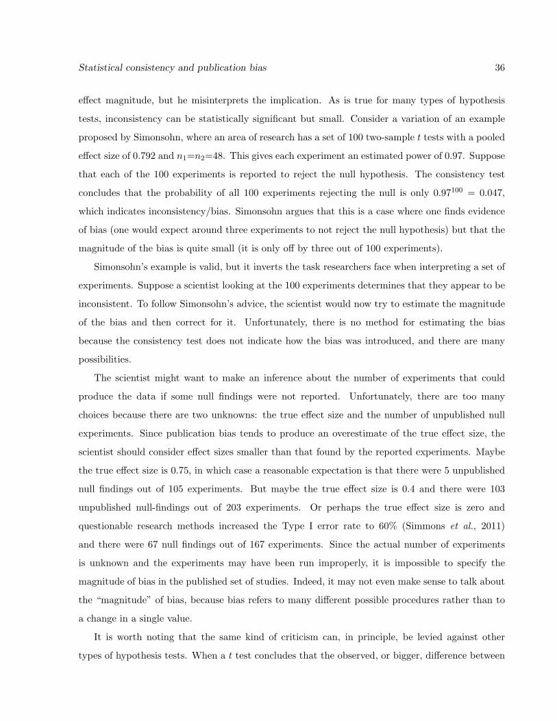
Statistical consistency and publication bias 36
e↵ect magnitude, but he misinterprets the implication. As is true for many types of hypothesis
tests, inconsistency can be statistically significant but small. Consider a variation of an example
proposed by Simonsohn, where an area of research has a set of 100 two-sample t tests with a pooled
e↵ect size of 0.792 and n1=n2=48. This gives each experiment an estimated power of 0.97. Suppose
that each of the 100 experiments is reported to reject the null hypothesis. The consistency test
concludes that the probability of all 100 experiments rejecting the null is only 0.97100 = 0.047,
which indicates inconsistency/bias. Simonsohn argues that this is a case where one finds evidence
of bias (one would expect around three experiments to not reject the null hypothesis) but that the
magnitude of the bias is quite small (it is only o↵ by three out of 100 experiments).
Simonsohn’s example is valid, but it inverts the task researchers face when interpreting a set of
experiments. Suppose a scientist looking at the 100 experiments determines that they appear to be
inconsistent. To follow Simonsohn’s advice, the scientist would now try to estimate the magnitude
of the bias and then correct for it. Unfortunately, there is no method for estimating the bias
because the consistency test does not indicate how the bias was introduced, and there are many
possibilities.
The scientist might want to make an inference about the number of experiments that could
produce the data if some null findings were not reported. Unfortunately, there are too many
choices because there are two unknowns: the true e↵ect size and the number of unpublished null
experiments. Since publication bias tends to produce an overestimate of the true e↵ect size, the
scientist should consider e↵ect sizes smaller than that found by the reported experiments. Maybe
the true e↵ect size is 0.75, in which case a reasonable expectation is that there were 5 unpublished
null findings out of 105 experiments. But maybe the true e↵ect size is 0.4 and there were 103
unpublished null-findings out of 203 experiments. Or perhaps the true e↵ect size is zero and
questionable research methods increased the Type I error rate to 60% (Simmons et al., 2011)
and there were 67 null findings out of 167 experiments. Since the actual number of experiments
is unknown and the experiments may have been run improperly, it is impossible to specify the
magnitude of bias in the published set of studies. Indeed, it may not even make sense to talk about
the “magnitude” of bias, because bias refers to many di↵erent possible procedures rather than to
a change in a single value.
It is worth noting that the same kind of criticism can, in principle, be levied against other
types of hypothesis tests. When a t test concludes that the observed, or bigger, di↵erence between
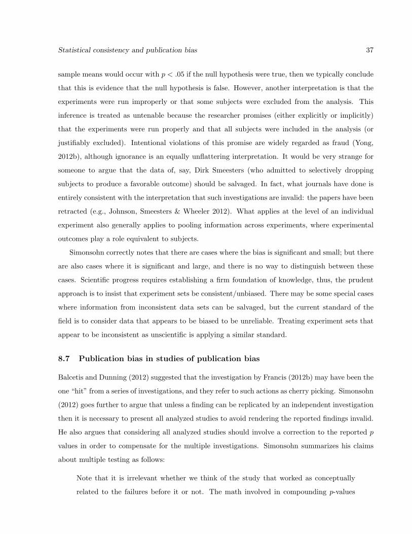
Statistical consistency and publication bias 37
sample means would occur with p < .05 if the null hypothesis were true, then we typically conclude
that this is evidence that the null hypothesis is false. However, another interpretation is that the
experiments were run improperly or that some subjects were excluded from the analysis. This
inference is treated as untenable because the researcher promises (either explicitly or implicitly)
that the experiments were run properly and that all subjects were included in the analysis (or
justifiably excluded). Intentional violations of this promise are widely regarded as fraud (Yong,
2012b), although ignorance is an equally unflattering interpretation. It would be very strange for
someone to argue that the data of, say, Dirk Smeesters (who admitted to selectively dropping
subjects to produce a favorable outcome) should be salvaged. In fact, what journals have done is
entirely consistent with the interpretation that such investigations are invalid: the papers have been
retracted (e.g., Johnson, Smeesters & Wheeler 2012). What applies at the level of an individual
experiment also generally applies to pooling information across experiments, where experimental
outcomes play a role equivalent to subjects.
Simonsohn correctly notes that there are cases where the bias is significant and small; but there
are also cases where it is significant and large, and there is no way to distinguish between these
cases. Scientific progress requires establishing a firm foundation of knowledge, thus, the prudent
approach is to insist that experiment sets be consistent/unbiased. There may be some special cases
where information from inconsistent data sets can be salvaged, but the current standard of the
field is to consider data that appears to be biased to be unreliable. Treating experiment sets that
appear to be inconsistent as unscientific is applying a similar standard.
8.7 Publication bias in studies of publication bias
Balcetis and Dunning (2012) suggested that the investigation by Francis (2012b) may have been the
one “hit” from a series of investigations, and they refer to such actions as cherry picking. Simonsohn
(2012) goes further to argue that unless a finding can be replicated by an independent investigation
then it is necessary to present all analyzed studies to avoid rendering the reported findings invalid.
He also argues that considering all analyzed studies should involve a correction to the reported p
values in order to compensate for the multiple investigations. Simonsohn summarizes his claims
about multiple testing as follows:
Note that it is irrelevant whether we think of the study that worked as conceptually
related to the failures before it or not. The math involved in compounding p-values
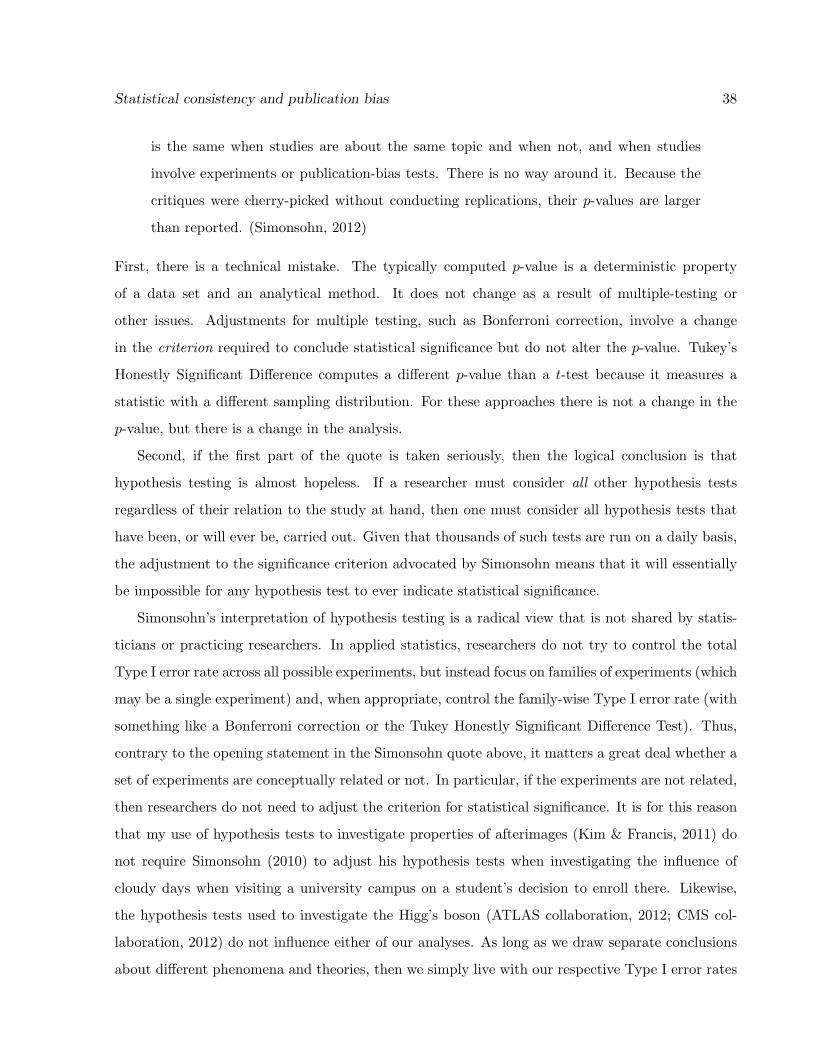
Statistical consistency and publication bias 38
is the same when studies are about the same topic and when not, and when studies
involve experiments or publication-bias tests. There is no way around it. Because the
critiques were cherry-picked without conducting replications, their p-values are larger
than reported. (Simonsohn, 2012)
First, there is a technical mistake. The typically computed p-value is a deterministic property
of a data set and an analytical method. It does not change as a result of multiple-testing or
other issues. Adjustments for multiple testing, such as Bonferroni correction, involve a change
in the criterion required to conclude statistical significance but do not alter the p-value. Tukey’s
Honestly Significant Di↵erence computes a di↵erent p-value than a t-test because it measures a
statistic with a di↵erent sampling distribution. For these approaches there is not a change in the
p-value, but there is a change in the analysis.
Second, if the first part of the quote is taken seriously, then the logical conclusion is that
hypothesis testing is almost hopeless. If a researcher must consider all other hypothesis tests
regardless of their relation to the study at hand, then one must consider all hypothesis tests that
have been, or will ever be, carried out. Given that thousands of such tests are run on a daily basis,
the adjustment to the significance criterion advocated by Simonsohn means that it will essentially
be impossible for any hypothesis test to ever indicate statistical significance.
Simonsohn’s interpretation of hypothesis testing is a radical view that is not shared by statis-
ticians or practicing researchers. In applied statistics, researchers do not try to control the total
Type I error rate across all possible experiments, but instead focus on families of experiments (which
may be a single experiment) and, when appropriate, control the family-wise Type I error rate (with
something like a Bonferroni correction or the Tukey Honestly Significant Di↵erence Test). Thus,
contrary to the opening statement in the Simonsohn quote above, it matters a great deal whether a
set of experiments are conceptually related or not. In particular, if the experiments are not related,
then researchers do not need to adjust the criterion for statistical significance. It is for this reason
that my use of hypothesis tests to investigate properties of afterimages (Kim & Francis, 2011) do
not require Simonsohn (2010) to adjust his hypothesis tests when investigating the influence of
cloudy days when visiting a university campus on a student’s decision to enroll there. Likewise,
the hypothesis tests used to investigate the Higg’s boson (ATLAS collaboration, 2012; CMS col-
laboration, 2012) do not influence either of our analyses. As long as we draw separate conclusions
about di↵erent phenomena and theories, then we simply live with our respective Type I error rates
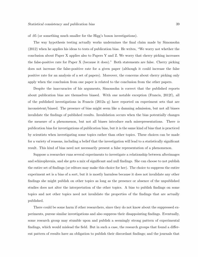
Statistical consistency and publication bias 39
of .05 (or something much smaller for the Higg’s boson investigations).
The way hypothesis testing actually works undermines the final claim made by Simonsohn
(2012) when he applies his ideas to tests of publication bias. He writes, “We worry not whether the
conclusion about Paper X applies also to Papers Y and Z. We worry that cherry picking increases
the false-positive rate for Paper X (because it does).” Both statements are false. Cherry picking
does not increase the false-positive rate for a given paper (although it could increase the false
positive rate for an analysis of a set of papers). Moreover, the concerns about cherry picking only
apply when the conclusion from one paper is related to the conclusion from the other papers.
Despite the inaccuracies of his arguments, Simonsohn is correct that the published reports
about publication bias are themselves biased. With one notable exception (Francis, 2012f), all
of the published investigations in Francis (2012a–g) have reported on experiment sets that are
inconsistent/biased. The presence of bias might seem like a damning admission, but not all biases
invalidate the findings of published results. Invalidation occurs when the bias potentially changes
the measure of a phenomenon, but not all biases introduce such misrepresentations. There is
publication bias for investigations of publication bias, but it is the same kind of bias that is practiced
by scientists when investigating some topics rather than other topics. These choices can be made
for a variety of reasons, including a belief that the investigation will lead to a statistically significant
result. This kind of bias need not necessarily present a false representation of a phenomenon.
Suppose a researcher runs several experiments to investigate a relationship between afterimages
and schizophrenia, and she gets a mix of significant and null findings. She can choose to not publish
the entire set of findings (or editors may make this choice for her). The choice to suppress the entire
experiment set is a bias of a sort, but it is mostly harmless because it does not invalidate any other
findings she might publish on other topics as long as the presence or absence of the unpublished
studies does not alter the interpretation of the other topics. A bias to publish findings on some
topics and not other topics need not invalidate the properties of the findings that are actually
published.
There could be some harm if other researchers, since they do not know about the suppressed ex-
periments, pursue similar investigations and also suppress their disappointing findings. Eventually,
some research group may stumble upon and publish a seemingly strong pattern of experimental
findings, which would mislead the field. But in such a case, the research groups that found a di↵er-
ent pattern of results have an obligation to publish their discordant findings; and the journals that

Statistical consistency and publication bias 40
published the positive findings have an obligation to publish the negative findings. If the e↵ect is
important, then researchers and journals need to promote accurate measurement of the e↵ect.
What is definitely not harmless is for a researcher to selectively report significant findings that
are all related to the same topic while suppressing null findings on that topic. If a researcher
investigates a relationship between afterimages and schizophrenia and gets some experiments that
reject the null and some experiments that do not, then it is improper for her to publish the
significant findings and not the null findings. Such choices would mischaracterize the relationship
between afterimages and schizophrenia.
These observations suggest that it may not be useful to consider publication bias for experiment
sets that do not address a common phenomenon or theory. For example, as noted by Sterling (1959),
Fanelli (2010), and others, the field of psychology has a preference for publishing statistically
significant findings. This selectivity is a bias, and many people interpret this finding to indicate
that there are serious problems in psychology (e.g., Bones, 2012; Simonsohn, 2012). But this kind
of bias does not necessarily indicate a problem. A plausible interpretation is that psychologists
want to read about (and/or journals want to publish) topics that tend to reject the null hypothesis.
Such a bias can exist even if almost all of the reported findings are themselves unbiased. (This
interpretation might be incorrect, but it is consistent with the findings of Sterling and others.)
The way to identify bias is topic-by-topic, because that is where the bias certainly misrepresents
the properties of reported findings. This topic-by-topic analysis characterizes the publication bias
analyses in Francis (2012a–g).
Curiously, the same kind of logic applies to a single experiment set that appears to have bias.
For example, Francis (2012b) showed that the experiment set in Balcetis and Dunning (2010) ap-
peared to be inconsistent/biased. This interpretation does not imply that each reported experiment
is invalid. It is possible that the reported experiments were run and analyzed properly and (individ-
ually) give a proper description of the investigated phenomenon. The problem with the findings in
Balcetis and Dunning (2010) is not (necessarily) with any individual reported experiment but with
the conclusion that is drawn across the set of experiments. With publication bias the experiment
set becomes invalid, even though the individual reported experiments might be fine in isolation.
The problem with the set hinges on the fact that the experiments in the set contribute toward
a common conclusion and should (but do not because of the apparent bias) give a better charac-
terization of the e↵ect than any individual experiment. The absence of a common conclusion is
Statistical consistency and publication bias 41
what di↵erentiates the bias in the publication bias reports by Francis (2012a–g) from the bias in
the findings of Balcetis and Dunning (and others). The investigation of publication bias in Balcetis
and Dunning (2010) is unrelated to the investigation of publication bias in Bem (2011), Pi↵ et al.
(2012), Galak and Meyvis (2011), or any other studies. It would not make sense to talk about a
conclusion across the sets of experiments that show publication bias because each experiment set
investigates a di↵erent phenomenon. Each of the consistency/bias investigations stands by itself,
so the bias that comes from selectively reporting some cases and not others does not invalidate
the reported findings. Of course, readers should not infer that since Francis (2012a–g) concludes
inconsistency/bias in, say, 90% of the reported analyses that 90% of the studies in psychology are
inconsistent. Neither should a reader infer that Francis has an ability to ferret out biased experi-
ment sets with an accuracy of 90%. Such inferences would be using the results to contribute to a
common conclusion, which is inappropriate.
Finally, although not central to the argument, it is worth noting that the bias among the
reported consistency/bias investigations is fundamentally di↵erent from the bias in the critiqued
studies. If another researcher wants to investigate the rate of publication bias across psychology
(or some subfield), all of the data are available. The fact that few of the investigations in Francis
(2012a–g) report about unbiased experiment sets does not prohibit other researchers from analyzing
such sets. Unlike the non-reporting of null experimental findings, where the data are not available
for anyone but the authors to consider, everyone is free to explore the properties of published
experiment sets. An unwillingness (or inability) to publish analyses of experiment sets that appear
to be without bias does not withhold any data from the field.
9 Conclusions
What has previously been called a test for an excessive number of significant findings (Ioannidis
& Trikalinos, 2007), a test for publication bias (Francis, 2012a), or an investigation of incredibility
(Schimmack, 2012) is really a test for consistency in a set of reported experiments. Consistency
is closely related to these other terms because a set of experiments that are run properly and
reported fully rarely leads to a conclusion of inconsistency. Experiment sets that are biased in
several di↵erent ways can lead to conclusions of inconsistency, although the test remains quite
conservative.
Statistical consistency and publication bias 42
The simulations and analyses in this paper clarify the connection between consistency and
various forms of publication bias. Unbiased sets only rarely produce inconsistent experiment sets
because even those sets that are unusual relative to the true e↵ect size are generally consistent with
the estimated e↵ect size. In contrast, biased experiment sets more frequently produce inconsistent
sets because the biasing process tends to produce experiments that just barely reject the null
hypothesis. Such sets tend to have low power relative to the reported replication rate.
The general principle of requiring consistency in experiment sets seems like an important con-
straint on how the field summarizes and reports empirical data. Unfortunately, this principle is
contrary to how many people have learned, taught, and practiced experimental psychology. This
conflict needs be resolved because many of the topics in psychology are truly important for in-
dividuals and for society. Application of the consistency test will hopefully motivate researchers
to perform better experiments, to understand the uncertainty in their data, and to winnow deep
truths from deep nonsense.
Acknowledgments
The author thanks Zyg Pizlo and Jim Nairne for valuable conversations on these topics.
Statistical consistency and publication bias 43
References
ATLAS collaboration (2012). Observation of a new particle in the search for the standard model
Higgs boson with the ATLAS detector at the LHC. Physics Letters B, 716(1), 1–29. arXiv:1207.7214.
doi:10.1016/j.physletb.2012.08.020.
Anscombe, F. J. (1954). Fixed-sample-size analysis of sequential observations. Biometrics, 10(1),
89–100.
Balcetis, E. & Dunning, D. (2010). Wishful seeing: More desired objects are seen as closer. Psy-
chological Science, 21(1), 147–152.
Balcetis E, & Dunning D. (2012) A false-positive error in search in selective reporting: A refutation
of Francis. i-Perception, 3, Author response.
Begg, C. B. & Mazumdar, M. (1994). Operating characteristics of a rank correlation test for
publication bias. Biometrics, 50, 1088–1101.
Bem, D. J. (2011). Feeling the future: Experimental evidence for anomalous retroactive influences
on cognition and a↵ect. Journal of Personality and Social Psychology, 100, 407–425.
Bones, A. K. (2012). We knew the future all along. Perspectives on Psychological Science, 7(3),
307–309. doi: 10.1177/1745691612441216
Borenstein, M., Hedges, L. V., Higgins, J. P. T., & Rothstein, H. R. (2009). Introduction to
meta-analysis. Chichester, UK: Wiley.
Champely, S. (2009). pwr: Basic functions for power analysis. R package version 1.1.1.
http://CRAN.R-project.org/package=pwr.
CMS collaboration (2012). Observation of a new boson at a mass of 125 GeV with the CMS
experiment at the LHC. Physics Letters B, 716 (1), 30–61.
arXiv:1207.7235. doi:10.1016/j.physletb.2012.08.021.
Cohen, J. (1988). Statistical Power Analysis for the Behavioral Sciences (2nd ed.). Hillsdale, NJ:
Erlbaum.
Statistical consistency and publication bias 44
Cumming, G. (2008). Replication and p intervals: p values predict the future only vaguely, but
confidence intervals do much better. Perspectives on Psychological Science, 3, 286–300.
Cumming, G. (2012). Understanding The New Statistics: E↵ect Sizes, Confidence Intervals, and
Meta-Analysis. New York: Routledge.
Duval S. & Tweedie R. (2000). Trim and fill: a simple funnel-plot-based method of testing and
adjusting for publication bias in meta-analysis. Biometrics, 56, 455–463.
Enserink, M. (2011). Dutch university sacks social psychologist over faked data. Science, http://
news.sciencemag.org/scienceinsider/2011/09/dutch-university-sacks-social.html
Fanelli, D. (2010) Positive Results Increase Down the Hierarchy of the Sciences. PLoS ONE, 5(4):
e10068. doi:10.1371/journal.pone.0010068
Francis, G. (2012a). Too good to be true: Publication bias in two prominent studies from experi-
mental psychology. Psychonomic Bulletin & Review, 19, 151–156.
Francis, G. (2012b). The same old New Look: Publication bias in a study of wishful seeing.
i-Perception, 3, 176–178.
Francis, G. (2012c). Response to author: Some clarity about publication bias and wishful seeing.
i-Perception, 3. doi 10.1068/i0519ic
Francis, G. (2012d). Evidence that publication bias contaminated studies relating social class and
unethical behavior. Proceedings of the National Academy of Sciences. 109, E1587
Francis, G. (2012e). Checking the counterarguments confirms that publication bias contaminated
studies relating social class and unethical behavior. Downloaded from
http://www1.psych.purdue.edu/⇠gfrancis/Publications/FrancisRebuttal2012.pdf
Francis, G. (2012f). Publication bias and the failure of replication in experimental psychology.
Psychonomic Bulletin & Review. doi: 10.3758/s13423-012-0322-y
Francis, G. (2012g). The psychology of replication and replication in psychology. Perspectives on
Psychological Science, 7(6), 580-589. doi: 10.1177/1745691612459520
Francis, G. (2013). Publication bias in Red, Rank, and Romance in Women Viewing Men by Elliot
et al. (2010). Journal of Experimental Psychology: General, 142(1), 292–296.

Statistical consistency and publication bias 45
Galak, J., LeBoeuf, R. A., Nelson, L. D. & Simmons, J. P. (2012). Correcting the past: Failures
to replicate Psi. Journal of Personality and Social Psychology, 103(6), 933–948.
Galak, J. & Meyvis, T. (2011). The pain was greater if it will happen again: The e↵ect of anticipated
continuation on retrospective discomfort. Journal of Experimental Psychology: General, 140,
63–75.
Galak, J. & Meyvis, T. (2011). (2012) You could have just asked: Reply to Francis (2012).
Perspectives on Psychological Science, 7(6), 595–596.
Gillett, R. (1994). Post hoc power analysis. Journal of Applied Psychology, 79, 783–785.
Hedges, L. V. (1981). Distribution theory for Glass’s estimator of e↵ect size and related estimators.
Journal of Educational Statistics, 6, 107–128.
Hedges, L. V. & Olkin, I. (1985). Statistical methods for meta-analysis. New York: Academic
Press.
Hoenig, J. M. & Heisey, D. M. (2001). The abuse of power: The pervasive fallacy of power
calculations for data analysis. American Statistician, 55, 19–24.
Ioannidis, J. P. A. (2008). Why most discovered true associations are inflated. Epidemiology, 19,
640–648.
Ioannidis, J. P. A. & Trikalinos T. A. (2007). An exploratory test for an excess of significant
findings. Clinical Trials, 4, 245–253.
John, L. K., Loewenstein, G., & Prelec, D. (2012). Measuring the prevalence of questionable
research practices with incentives for truth-telling. Psychological Science, 23, 524–532.
Johnson, C. S., Smeesters, D., Wheeler, S. C. (2012). Retraction of Johnson, Smeesters, and
Wheeler (2012). Journal of Personality and Social Psychology, 103(4), 605.
Johnson, V. & Yuan, Y. (2007). Comments on An exploratory test for an excess of significant
findings by JPA loannidis and TA Trikalinos. Clinical Trials, 4, 254–255.
Kelley, K. (2007). Confidence intervals for standardized e↵ect sizes: Theory, application, and
implementation. Journal of Statistical Software, 20. http://www.jstatsoft.org/v20/a08/

Statistical consistency and publication bias 46
Kerr, N. L. (1998). HARKing: Hypothesizing After the Results are Known. Personality and Social
Psychology Review, 2, 196–217.
Kim, J. & Francis, G. (2011). Color selection, color capture, and afterimage filling-in. Journal of
Vision, 11(3):22, http://www.journalofvision.org/content/11/3/23/, doi:10.1167/11.3.23.
Kline, R. B. (2004). Beyond significance testing: Reforming data analysis methods in behavioral
research. Washington, DC: American Psychological Association.
Kruschke, J. K. (2010a). Bayesian data analysis. Wiley Interdisciplinary Reviews: Cognitive
Science, 1(5), 658–676. doi:10.1002/wcs.72
Kruschke, J. K. (2010b). Doing Bayesian Data Analysis: A Tutorial with R and BUGS. Academic
Press/Elsevier Science.
Lane, D. M. & Dunlap, W. P. (1978). Estimating e↵ect size: Bias resulting from the significance
criterion in editorial decisions. British Journal of Mathematical and Statistical, Psychology, 31,
107–112.
Meehl, P. E. (1978). Theoretical risks and tabular asterisks: Sir Karl, Sir Ronald, and the slow
progress of soft psychology. Journal of Consulting and Clinical Psychology, 46, 806–834.
Miller, J. (2009). What is the probability of replicating a statistically significant e↵ect? Psycho-
nomic Bulletin & Review, 16, 617–640.
Pashler, H., & Wagenmakers, E.-J. (2012). Editors’ introduction to the special section on replica-
bility in psychological science: A crisis of confidence? Perspectives on Psychological Science, 7,
528–530.
Peters, J. L., Sutton, A. J., Jones, D. R., Abrams, K. R. & Rushton, L. (2007). Performance of
the trim and fill method in the presence of publication bias and between-study heterogeneity
Statistics in Medicine, 26, 4544–4562.
Phillips, C. V. (2004). Publication bias in situ. BMC Medical Research Methodology, 4(20).
doi:10.1186/1471-2288-4-20
Statistical consistency and publication bias 47
Pi↵, P. K., Stancato, D. M., Cote, S., Mendoza-Denton, R., & Keltner, D. (2012a). Higher social
class predicts increased unethical behavior. Proceedings of the National Academy of Sciences
USA, 109, 4086– 4091. doi/10.1073/pnas.1118373109
Pi↵, P. K., Stancato, D. M., Cote, S., Mendoza-Denton, R. & Keltner, D. (2012b). Reply to Francis:
Cumulative power calculations are faulty when based on observed power and a small sample of
studies. Proceedings of the National Academy of Sciences USA. doi:10.1073/pnas.1205367109
R Development Core Team. (2011) R: A language and environment for statistical computing. R
Foundation for Statistical Computing, Vienna, Austria. ISBN 3-900051-07-0, http://www.R-
project.org/.
Ritchie, S. J., Wiseman, R., & French, C. C. (2012). Failing the future: Three unsuccessful
attempts to replicate Bem’s ‘retroactive facilitation of recall’ e↵ect. PLoS ONE, 7(3): e33423.
doi:10.1371/journal.pone.0033423
Roediger, H. L. (2012). Psychology’s woes and a partial cure: The value of replication. APS Ob-
server, 25, No. 2. http://www.psychologicalscience.org/index.php/publications/observer/2012/
february-11-2012-observer-publications/psychologys-woes-and-a-partial-cure-the-value-of
-replication.html
Rosenthal, R. (1984). Applied Social Research Methods Series, Vol. 6. Meta-analytic procedures
for social research. Newbury Park, CA: Sage Publications.
Scargle, J. D. (2000). Publication bias: The File-Drawer problem in scientific inference. Journal
of Scientific Exploration, 14(1), 91–106.
Sagan, C. (1997). The Demon-Haunted World: Science as a Candle in the Dark. New York:
Ballantine Books.
Schimmack, U. (2012). The ironic e↵ect of significant results on the credibility of multiple study
articles. Psychological Methods. Advance online publication. doi: 10.1037/a0029487
Shea, C. (2011). Fraud scandal fuels debate over practices of social psychology. The Chron-
icle of Higher Education. Downloaded from http://chronicle.com/article/As-Dutch-Research-
Scandal/129746/

Statistical consistency and publication bias 48
Simmons, J. P., Nelson, L. D., & Simonsohn, U. (2011). False-positive psychology: Undisclosed
flexibility in data collection and analysis allows presenting anything as significant. Psychological
Science, 22, 1359–1366.
Simonsohn, U. (2010). Weather to go to college. The Economic Journal, 120(543), 270–280.
Simonsohn, U. (2012) It does not follow: Evaluating the one-o↵ publication bias critiques by Francis
(2012a,b,c,d,e,f), Perspectives on Psychological Science, 7(6), 597–599.
Sterling, T. D. (1959). Publication decisions and the possible e↵ects on inferences drawn from test
of significance–or vice versa. Journal of the American Statistical Association, 54, 30–34.
Sterne, J. A., Gavaghan, D. & Egger, M. (2000). Publication and related bias in meta-analysis:
Power of statistical tests and prevalence in the literature. Journal of Clinical Epidemiology, 53,
1119–1129.
Thompson, B. (2006). Foundations of behavioral statistics: An insight-based approach. New York:
Guilford.
Topolinski, S. & Sparenberg, P. (2012). Turning the hands of time: Clockwise movements increase
preference for novelty. Social Psychological and Personality Science, 3, 308–314.
Wagenmakers, E.-J. (2007). A practical solution to the pervasive problems of p values. Psycho-
nomic Bulletin & Review, 14, 779–804.
Wagenmakers, E.-J., Wetzels, R., Borsboom, D., & van der Maas, H. L. J. (2011). Why psychol-
ogists must change the way they analyze their data: The case of psi: Comment on Bem (2011).
Journal of Personality and Social Psychology, 100, 426–432.
Yong, E. (2012a). Bad copy. Nature, 485, 298–300.
Yong, E. (2012b). The data detective. Nature, 487, 18–19, doi:10.1038/487018a.
Yuan, K. H. & Maxwell, S. (2005). On the post hoc power in testing mean di↵erences. Journal of
Educational and Behavioral Statistics, 30, 141–167.