renewable fuels module of the national energy modeling

Renewable Fuels Module of the National Energy Modeling System: Model Documentation 2020 June 2020

Independent Statistics & Analysis www.eia.gov

U.S. Department of Energy

Washington, DC 20585

U.S. Energy Information Administration | Renewable Fuels Module of the National Energy Modeling System: Model Documentation 2020 ii

This report was prepared by the U.S. Energy Information Administration (EIA), the statistical and analytical agency within the U.S. Department of Energy. By law, EIA’s data, analyses, and forecasts are independent of approval by any other officer or employee of the United States Government. The views in this report therefore should not be construed as representing those of the U.S. Department of Energy or other federal agencies.

June 2020

U.S. Energy Information Administration | Renewable Fuels Module of the National Energy Modeling System: Model Documentation 2020 ii

Update Information This edition of the Renewable Fuels Module—Model Documentation 2020 reflects changes made to the Renewable Fuels Module during the past year for the Annual Energy Outlook 2020. These changes include the following:

• Updated REStore submodule to provide an integrated 24-hour, 12-month (24 x 12) dispatching model resolution to account for chronological interactions for onshore wind, solar photovoltaic, and diurnal storage technologies. Also included peak-day timeslice and adjusted arbitrage value for diurnal storage.

• Updated capacity credit for wind and solar technologies based on a higher 24 x 12 time resolution. • Implemented a new parameter to better characterize spinning reserves to accommodate

increased wind and solar penetration. • Improved curtailment code. • Updated the short-term elasticity algorithm to account for a more gradual loss of market memory. • Established high-voltage direct current (HVDC) transmission capacity expansion to accommodate

high penetration of renewable generating capacity. • Revised the heat rate for renewables to reflect the average heat rate for current capacity

expansion year rather than the static initial value. • Updated POLYSYS submodule to reflect the most current model and input assumptions based on

University of Tennessee and the U.S. Department of Energy’s (DOE) Office of Energy Efficiency & Renewable Energy most recent 2016 Billion-Ton Report.

• Updated conventional hydroelectric supply curves based on the most recent Oak Ridge National Laboratory study on non-powered dams.

• Reallocated renewable resources to match the revised Electricity Market Module’s region definitions, including regional cost multipliers.

• Revised accounting for Renewable Portfolio Standard generation to account for interregional trade.

June 2020

U.S. Energy Information Administration | Renewable Fuels Module of the National Energy Modeling System: Model Documentation 2020 iii

Contents Update Information ...................................................................................................................................... ii

Tables ........................................................................................................................................................... vi

1. Introduction .............................................................................................................................................. 2

Purpose of this report .............................................................................................................................. 2

Renewable Fuels Module summary ........................................................................................................ 2

Representation of depreciation for renewables-fueled generating technologies .................................. 5

Report organization ................................................................................................................................. 6

2. Capacity credit for intermittent generation ............................................................................................. 7

Appendix 2-A: Background information on the capacity credit algorithm for intermittent generation .... 11

3. Landfill Gas (LFG) Submodule ................................................................................................................. 19

Model purpose ...................................................................................................................................... 19

Relationship of the LFG Submodule to other models............................................................................ 19

Modeling rationale ................................................................................................................................ 19

Fundamental assumptions .................................................................................................................... 19

LFG Submodule structure ...................................................................................................................... 22

Appendix 3-A: Inventory of Variables, Data, and Parameters .................................................................... 24

Appendix 3-B: Mathematical Description ................................................................................................... 28

Appendix 3-C: Bibliography ......................................................................................................................... 30

Appendix 3-D: Model Abstract .................................................................................................................... 31

Appendix 3-E: Data Quality and Estimation Processes ............................................................................... 33

4. Wind Energy Submodule (WES) .............................................................................................................. 34

Model purpose ...................................................................................................................................... 34

Relationship of the Wind Energy Submodule to other models ............................................................. 34


Offshore wind .................................................................................................................................. 36


Cost adjustment factors ......................................................................................................................... 41

Alternative approaches.......................................................................................................................... 43

Wind Energy Submodule structure........................................................................................................ 43



June 2020

U.S. Energy Information Administration | Renewable Fuels Module of the National Energy Modeling System: Model Documentation 2020 iv




5. Solar Submodule ..................................................................................................................................... 63

Model purpose ...................................................................................................................................... 63

Relationship of the Solar Submodule to other models ......................................................................... 63



Short-term cost adjustment factors ...................................................................................................... 64

Solar Submodule structure .................................................................................................................... 64






6. Biomass Submodule ................................................................................................................................ 76

Model purpose ...................................................................................................................................... 76

Relationship of the Biomass Submodule to other models .................................................................... 76



Alternative approaches.......................................................................................................................... 77

Biomass Submodule structure ............................................................................................................... 78






7. Geothermal Electricity Submodule ......................................................................................................... 93

Model purpose ...................................................................................................................................... 93

Relationship of the Geothermal Electricity Submodule to other models ............................................. 93



June 2020

U.S. Energy Information Administration | Renewable Fuels Module of the National Energy Modeling System: Model Documentation 2020 v

Geothermal Electricity Submodule structure ........................................................................................ 96

Key computations and equations .......................................................................................................... 97

Appendix 7-A: Inventory of Variables, Data, and Parameters .................................................................. 101

Appendix 7-B: Mathematical Description ................................................................................................. 102

Appendix 7-C: Bibliography ....................................................................................................................... 104

Appendix 7-D: Model Abstract .................................................................................................................. 106

8. Conventional Hydroelectricity Submodule ........................................................................................... 108

Model purpose .................................................................................................................................... 108

Fundamental assumptions .................................................................................................................. 109

Alternative approaches........................................................................................................................ 113

Conventional Hydroelectricity Submodule structure .......................................................................... 113

Key computations and equations ........................................................................................................ 115

Appendix 8-A: Inventory of Variables, Data, and Parameters .................................................................. 119

Appendix 8-B: Mathematical Description ................................................................................................. 120

Appendix 8-C: Bibliography ....................................................................................................................... 121

Appendix 8-D: Model Abstract .................................................................................................................. 122

June 2020

U.S. Energy Information Administration | Renewable Fuels Module of the National Energy Modeling System: Model Documentation 2020 vi

Tables Table 2-2. Forced outage rate by major group of NEMS capacity type ...................................................... 16 Table 2-3. Regional power correlation factors (dimensionless) ................................................................. 17 Table 4-3. Learning parameter for wind turbine capacity factor ............................................................... 41 Table 3-1. Methane production parameters for high, low, and very low yield sites.................................. 21 Table 3A-1. NEMS landfill gas submodule inputs and outputs ................................................................... 24 Table 4A-1. NEMS wind energy submodule inputs and outputs ................................................................ 45 Table 4-1. Wind class .................................................................................................................................. 37 Table 4-2. Transmission costs by region ........................................................ Error! Bookmark not defined. Table 6A-1. NEMS Biomass Submodule inputs and variables..................................................................... 80

June 2020

U.S. Energy Information Administration | Renewable Fuels Module of the National Energy Modeling System: Model Documentation 2020 vii

Figures

Figure 1. Potential shift in peak net-load within a day ............................................................................... 13 Figure 2. Power output from a typical wind turbine as a function of ambient wind speed ....................... 14 Figure 3. Weibul probability density function with a shape parameter of 2 .............................................. 15 Figure 4. Landfill Gas Submodule flowchart ............................................................................................... 22 Figure 5. Wind Energy Submodule flowchart ............................................................................................. 44 Figure 6. Solar Energy Submodule flowchart .............................................................................................. 65 Figure 7. Biomass Submodule flowchart .................................................................................................... 79

June 2020

U.S. Energy Information Administration | Renewable Fuels Module of the National Energy Modeling System: Model Documentation 2020 2

1. Introduction

Purpose of this report This report documents the objectives, analytical approach, and design of the National Energy Modeling System (NEMS) Renewable Fuels Module (RFM) as it relates to the production of the Annual Energy Outlook 2020 (AEO2020) forecasts. The report catalogues and describes modeling assumptions, computational methodologies, data inputs, and parameter estimation techniques. A number of off-line analyses used in place of RFM modeling components are also described.

This documentation report serves three purposes. First, it is a reference document for model analysts, model users, and the public interested in the construction and application of the RFM. Second, it meets the legal requirement of the U.S. Energy Information Administration (EIA) to provide adequate documentation in support of its models (Public Law 93-275, Federal Energy Administration Act of 1974, Section 57(b) (1)). Third, such documentation facilitates continuity in EIA model development by providing information sufficient to perform model enhancements and data updates as part of EIA's ongoing mission to provide analytical and forecasting information systems.

Renewable Fuels Module summary The RFM consists of six submodules that represent major renewable electricity resources: biomass, landfill gas (LFG), solar (thermal and photovoltaic), wind, geothermal, and conventional hydroelectricity energy. The RFM also interacts with the REStore model to estimate the impact of energy storage on the dispatch of generation in each of the modeled electricity regions. The details of the REStore model are provided as an appendix to the Electricity Market Module (EMM) model documentation.

The purpose of the RFM is to define the technology, cost, performance, and renewable resource supply for renewable electricity technologies in the NEMS. The RFM estimations are provided to the EMM for use in projecting grid-connected central station electricity capacity planning and dispatch decisions. Projected characteristics include available generating capacity, location, unit size, capital cost, fixed operating cost, variable operating cost, capacity factor, heat rate, construction lead time, and fuel price. Because of the extensive interaction between the RFM, REStore, and EMM, these three modules must be run together.

Renewable electricity technology cost and performance characteristics that are common to all electricity-generating technologies are input directly to the EMM via the input file ECPDAT. Unique characteristics such as renewable resource values for regional, seasonal, and hourly time segments of intermittent renewables are supplied in specific files and subroutines to specific renewable electricity technologies.

Other renewables modeled elsewhere in NEMS include biomass in the industrial sector, biofuels in the Liquid Fuels Market Module (LFMM), wood and solar hot water heating in the residential sector, and geothermal heat pumps and distributed (grid-connected) solar photovoltaics in the residential and commercial sectors. In addition, several areas, primarily nonelectric and off-grid electric applications, are not represented in NEMS. They include direct applications of geothermal heat, several types of solar thermal use, and off-grid photovoltaics. For the most part, the expected contributions from these

June 2020


sources are confined to niche markets; however, as these markets develop in importance they will be considered for representation in NEMS.

The number and purpose of the associated technology and cost characteristics vary from one RFM submodule to another depending on the modeling context. For example, renewable resources such as solar, wind, and geothermal energy are not fuels; rather, they are inputs to electricity or heat conversion processes. Consequently, the Solar Submodule, Wind Submodule, and Geothermal Submodule do not provide fuel product prices.

EIA’s Office of Electricity, Coal, Nuclear, and Renewables Analysis determines initial cost and performance values for renewable electricity technologies based on the examination of available information. For AEO2020, the cost and performance characteristics for all generating technologies, including non-renewables, were re-evaluated and updated. The cost and performance characteristics include capital costs (excluding the construction financing and process and project contingency components that are provided in the EMM), fixed and variable operation & maintenance (O&M) costs, capacity factors, and construction lead times. All cost values are converted to 1987 dollars.

Provided below are summaries of the six RFM submodules that are used to produce the current forecasts: the Landfill Gas Submodule (LFG), the Wind Energy Submodule (WES), the Solar Energy Submodule (SOLAR), the Biomass Submodule, the Geothermal Energy Submodule (GES), and the Conventional Hydroelectricity Submodule (CHS). Each chapter concludes with information on the RFM archival package and EIA point of contact.

Landfill Gas Submodule (LFG) The Landfill Gas Submodule provides annual projections of energy produced from estimates of U.S. landfill gas capacity. The submodule calculates the quantity of LFG produced, derived from an econometric equation that uses gross domestic product (GDP) and U.S. population as the principal drivers. The LFG capacity is estimated based on reported waste and gas production data and judgment about future trends in recycling. The submodule uses LFG supply curves to reflect competition between new LFG-to-electricity capacity and other technologies in each projection period. The supply curves account for the amounts of high, low, and very low methane producing landfills located in each EMM region.

Wind Energy Submodule (WES) The Wind Energy Submodule (WES) projects the availability of wind resources. Projected undeveloped wind resource availability, expressed as megawatts (MW) of capacity in each region, is passed to the EMM, which models the building and dispatching of wind turbines in competition with other electricity-generating technologies. The wind turbine data are expressed in the form of energy supply curves. The supply curves provide the estimated maximum amount of turbine generating capacity that could be installed, given the available land area, average wind speed, and capacity factor. These variables are

June 2020


passed to the EMM in the form of nine time segments that are matched to electricity load curves within the EMM.1

Solar Submodule (SOLAR) Two solar technologies are represented in NEMS: a 150 MW single-axis tracking grid-connected central station photovoltaic (PV) unit without energy storage and a 100 MW central receiver (power tower) solar thermal unit (also called concentrating solar power, or CSP) also without energy storage. Both technologies are grid-connected and provided by electric utilities, small power producers, or independent power producers.

PV and solar thermal electric cost and performance characteristics are defined consistently with characteristics of fossil and other fuels reside in the ECPDAT input file. Performance characteristics unique to solar technologies (such as season and region-dependent capacity factors), however, are passed to the EMM via the Solar Submodule (SOLAR).

Biomass Submodule The Biomass Submodule provides biomass resource and technology cost and performance characteristics for a biomass burning electricity-generating technology to the EMM. The technology currently modeled is a direct combustion system. The submodule uses a regional biomass supply schedule from which the biomass fuel price is determined; fuel prices are added to variable operating costs because renewable fuels have no fuel costs in the NEMS structure. The biomass supply schedule is based on the accessibility of wood resources by the consuming sectors from existing wood and wood residues, crop residues, and energy crops. The LFMM also accesses the biomass supply curve to determine availability of feedstocks for production of cellulosic ethanol, biomass pyrolysis oils, and biomass-to-liquids. Projected feedstocks for production of sugar- or starch-based ethanol (primarily from corn, or maize, in the United States) are determined within the LFMM.

Geothermal Energy Submodule (GES) The Geothermal Energy Submodule (GES) models current and future regional supply, capital cost, and operation and maintenance costs of electric-generating facilities using hydrothermal resources (hot water and steam) and so-called near-field enhanced geothermal systems (EGS) sites, which are areas around the hydrothermal sites with high temperatures but less fluid. The data are assembled from 125 known hydrothermal sites and the 125 corresponding near-field EGS areas, each represented by information that reflects the specific resource conditions of that location. The GES generates a three-part geothermal resource supply curve for geothermal capacity for each region in each forecast year for competition with fossil-fueled and other generating technologies.

Conventional Hydroelectricity Submodule (CHS) The Conventional Hydroelectricity Submodule (CHS) models the supply (MW), capital cost, and operation and maintenance costs of conventional hydroelectric power available from adding new hydro generating capacity in increments of 1 MW or greater to new sites without dams, sites with existing dams but without hydroelectricity, and existing hydroelectricity sites able to accommodate additional

1 The nine time segments are derived from three eight-hour segments of the day for three seasons: winter, summer, and off-peak (spring/fall averaged). The data represent average capacities based on empirical analysis.

June 2020


capacity. The CHS uses the Idaho Hydropower Resource Economics Database (IHRED). The CHS does not account for pumped storage capacity, increments of capacity less than 1 MW, available from refurbishing and upgrading existing hydro capacity, or capacity available from new in-stream, offshore, or ocean technologies. Within each NEMS region, for each NEMS cycle, the CHS first identifies additional hydro capacity available at or less than an avoided cost specified by the EMM. It then segments the available capacity into three cost categories: lowest cost, midrange cost, and highest cost. The CHS then submits the MW of available capacity, expressed as average capital cost and operation and maintenance costs, each weighted by nameplate capacity, and capacity factors to the EMM for each of the three cost categories. After projecting capacity change decisions, the EMM informs the CHS of required decrements to potential available for selection in the next NEMS cycle.

Renewable Storage Submodule (REStore) The Renewable Storage Submodule (REStore) models the value of new energy storage capacity, dispatch of existing generation capacity, and curtailments of intermittent renewable technologies at a temporal resolution of 576 representative hours per year (12 months, 2 day types, 24 hours). The EMM takes the hourly generation output from REStore and aggregates it into the nine EMM time slices to determine the generation of intermittent renewable technologies, hydroelectric power, pumped hydro storage, and four-hour battery storage by region and model year. EMM also uses value of storage provided by REStore when making its capacity planning decisions. The RFM uses the hourly generation profile provided by REStore to determine the hourly capacity factor of intermittent renewable technologies in its capacity credit calculation. REStore does not reside within RFM, but it interacts directly with both RFM and EMM.

Capacity credit for intermittent generation Because there is a significant probability that at least some intermittent generators will be available during peak-demand periods as well as a significant probability that some portion of operator-dispatched capacity will not be available during that time, intermittent generators can contribute some fraction of their rated capacity to the reserve margin. This fraction, referred to as the capacity credit, is a function of the correlation between the temporal generation pattern of the resource and the peak-load periods, as well as the fraction of intermittent generation compared with total regional output. It is determined in NEMS as a function of the estimated average contribution that all intermittent units will provide to meet an assumed system reliability goal of 99.999% availability. This contribution is, in turn, largely determined by the average, peak-load period capacity factor for the intermittent capacity, the standard deviation around that average, the degree to which the output at each individual site in a region is correlated with the output at other sites, and the reliability characteristics of the operator-dispatched (conventional) capacity in the region.

Representation of depreciation for renewables-fueled generating technologies For most central station electricity-generating technologies, NEMS assumes a 20-year tax life during which the capital is depreciated. However, nuclear technologies are assigned a 15-year tax life. Renewables-fueled central station electricity-generating technologies—including biomass, geothermal, hydroelectric, landfill gas, solar (photovoltaic and thermal), and wind—are assigned five-year tax lives and five-year double declining balance depreciation in NEMS. Biomass, geothermal, solar, and wind have a five-year double declining balance depreciation as a result of the Economic Recovery Tax Act of

June 2020


1982 (ERTA, P.L. 97-34); see Internal Revenue Code, subtitle A, Chapter 1, Subchapter B, Part VI, Section 168 (e)(3)(vi)(1994)—accelerated cost recovery.

Archival Media The RFM is archived as part of the NEMS production runs.

Model Contact Chris Namovicz, Team Leader Renewable Electricity Analysis Team Office of Electricity, Coal, Nuclear, and Renewables Analysis U.S. Energy Information Administration, EI-34 1000 Independence Ave., SW Washington, DC 20585 Phone: (202) 586-7120 Email: [email protected]

Report organization Subsequent chapters of this report provide detailed documentation of each of the RFM's six working submodules. Each chapter contains the following sections:

• Model Purpose—a summary of the submodule's objectives, detailing input and output quantities, and the relationship of the submodule to other NEMS modules

• Model Rationale—a discussion of the submodule's design rationale, including insights into assumptions used in the model development process, and alternative modeling methodologies considered during the submodule development phase

• Model Structure—an outline of the model structure, using text and graphics to illustrate the major model data flows and key computations

This report also contains appendixes—supporting documentation for input data and parameter files currently residing on the EIA computer network. Appendix A in each RFM submodule chapter lists and defines the input data used to generate parameters and endogenous projections. Appendix B contains a mathematical description of the computation algorithms, including model equations and variable transformations. Appendix C is a bibliography of reference materials used in the model development process. Appendix D is a model abstract. Appendix E discusses data quality and estimation methods.

June 2020


2. Capacity credit for intermittent generation Within the EMM, each region must have enough generating capacity installed to satisfy peak-load requirements plus a regional reserve margin. For operator-dispatched capacity types, the summer-rated capacity for each generator unit is used to determine the contribution provided to the reserve margin requirement. However, non-dispatched and intermittently available generating capacity, such as wind turbines or solar electric facilities, will not always generate during peak-demand periods and thus cannot contribute its full rated capacity to satisfy the reserve margin requirement.

Because there is a significant probability that at least some intermittent generators will be available during peak-demand periods as well as a significant probability that some portion of operator-dispatched capacity will not be available during this time, intermittent generators can contribute some fraction of their rated capacity to the reserve margin. This fraction, referred to as the capacity credit, is a function of the correlation between the temporal generation pattern of the resource and the peak-load periods, as well as the fraction of intermittent generation compared with total regional output. That is, a wind turbine in a region where the wind typically blows strongly during the peak-load period will contribute more to meeting peak-load system reliability than a wind turbine in a region with typically light peak-load winds. However, as wind or solar constitutes more of the system capacity, the variability of the peak-load operation will have a decreasingly beneficial effect on system reliability.

The capacity credit for intermittent generators is determined in NEMS as a function of the estimated average contribution that all units of that type (wind or solar) will provide to meeting an assumed system reliability goal of 99.999% availability (that is, the system should have enough generation capacity installed to be able to meet full load requirements 99.999% of the time, sometimes approximated as achieving 1 hour of load shortage in 10 years, or 87,600 hours of operation). This contribution is, in turn, largely determined by the average, peak-load period capacity factor for the intermittent capacity, by the standard deviation around that average, by the degree to which the output at each individual site in a region is correlated with the output at other sites, and by the reliability characteristics of the operator-dispatched (conventional) capacity in the region.

The peak-load period capacity factor for each intermittent generator is determined as described in the Wind Energy Submodule and Solar Energy Submodule chapters of this report. The normalized standard deviations for wind and solar plants are exogenously determined. The intersite output correlation factors are also exogenously determined on a regional basis. The standard deviation for each conventional capacity type is calculated from the user-specified forced-outage rates, based on a binomial distribution:

( )N

PPCS )1( −××=

where;

C = the installed capacity of a specified type as calculated for that year

P = the forced outage rate (variable name UPFORT in the ECPDAT file)

June 2020


N = the number of units for the specified plant type as calculated for that year and region.

The standard deviation of total capacity of all conventional types is calculated as follows:

222

21 ... nalConvention SSSS ++=

where;

Sn =the standard deviation for the nth capacity type.

The standard deviation for all intermittent units of a specified type (wind, solar thermal, or photovoltaic) is determined as follows:

222 **)(* sRNNsNCS ntIntermitte −+×=

where;

s = the technology-specific normalized standard deviation of hourly output for intermittent resource facilities (INTSTDDV variable in the WESAREA file)

N and C = as above (for intermittent rather than conventional capacity types)

R = the regional correlation factor for intermittent resources (INTREGCRL variable in the WESAREA file).

The total standard deviation of all generation (conventional and intermittent) is then calculated as follows:

2222

21 ... ntIntermittenTotal SSSSS +++= ,

where;

Sn = as above

SIntermittent = the total standard deviation for the intermittent capacity type being evaluated (wind, solar thermal, or photovoltaic).

The reliable capacity is then calculated excluding the intermittent capacity, then again including all capacity types using the following:

( ) SZCCreliable ×−= ∑ n ave, ,

where;

Cave,n = the total annual average capacity for the nth capacity type and is evaluated for conventional-only capacity types and then again for conventional plus intermittent capacity types. For conventional resources, average capacity is the installed summer capacity multiplied

June 2020


by one minus the forced outage rate. For intermittent resources, it is the installed capacity times the peak-load period capacity factor.

Z = the statistical parameter for the number of standard deviations in a normal distribution that are needed to account for a specified fraction of the area under the distribution curve, specified as variable UPINTZ in the ECPDAT file2

S = as calculated above for Sconventional or STotal as appropriate for the conventional-only or the total reliable capacity calculation.

Although the approach above accounts for the impacts of spatial diversity of resource on available capacity, it does not account for the tendency of variable renewable energy resources (VRE), especially solar but to a lesser extent wind, to saturate certain time-of-day or seasonal demand hours. In particular, the net-load, or total demand minus average expected VRE generation, can decrease in a given hour of the day, month, or year once sufficient VRE generation from a particular source gets sufficiently large.

The net-load algorithm is used to reduce peak-load overestimation by accounting for the impact that the VRE generation has in suppressing effective demand to dispatchable generators during periods when the VRE is generating. The net-load curve is updated in each model year to represent the current penetration of the intermittent technology when calculating the capacity factor (see Appendix 1-A).

For each applicable intermittent resource, the capacity credit (U) is calculated as follows:

𝑈𝑈𝐼𝐼𝐼𝐼𝐼𝐼𝐼𝐼𝐼𝐼𝐼𝐼𝐼𝐼𝐼𝐼𝐼𝐼𝐼𝐼𝐼𝐼𝐼𝐼 =𝐶𝐶𝐼𝐼𝐼𝐼𝑟𝑟𝐼𝐼𝑟𝑟𝑟𝑟𝑟𝑟𝐼𝐼,𝐼𝐼𝐼𝐼𝐼𝐼 − 𝐶𝐶𝐼𝐼𝐼𝐼𝑟𝑟𝐼𝐼𝑟𝑟𝑟𝑟𝑟𝑟𝐼𝐼,𝑐𝑐𝑐𝑐𝐼𝐼𝑐𝑐𝐼𝐼𝐼𝐼𝐼𝐼𝐼𝐼𝑐𝑐𝐼𝐼𝑟𝑟𝑟𝑟

𝐶𝐶𝐼𝐼𝐼𝐼𝑖𝑖𝐼𝐼𝑟𝑟𝑟𝑟𝑟𝑟𝐼𝐼𝑖𝑖,𝐼𝐼𝐼𝐼𝐼𝐼𝐼𝐼𝐼𝐼𝐼𝐼𝐼𝐼𝐼𝐼𝐼𝐼𝐼𝐼𝐼𝐼𝐼𝐼

where;

Creliable = as above for net and conventional-only generation

Cintalled,Intermittent = the installed, nameplate capacity of the intermittent resource being evaluated (wind, solar thermal, or PV). Note that the capacity credit for each intermittent resource is evaluated separately. As a given intermittent resource is calculated, the other two are included in the conventional capacity calculations, using the capacity credit from the previous model iteration to determine availability.

Finally, for each VRE technology in each year, the capacity credit is updated by weighting the hours closest to the net peak that receive more than the hours further from the net peak:

𝑤𝑤𝑤𝑤𝑤𝑤ℎ = 𝑑𝑑𝑑𝑑𝑑𝑑𝑤𝑤𝑤𝑤𝑤𝑤 ∗ (𝑛𝑛𝑛𝑛𝑤𝑤 𝑙𝑙𝑙𝑙𝑑𝑑𝑑𝑑ℎ /𝑚𝑚𝑑𝑑𝑚𝑚 𝑛𝑛𝑛𝑛𝑤𝑤 𝑙𝑙𝑙𝑙𝑑𝑑𝑑𝑑) 𝑐𝑐𝑐𝑐𝐼𝐼𝑐𝑐𝑐𝑐

𝑐𝑐𝑑𝑑𝑐𝑐 𝑐𝑐𝑐𝑐𝑛𝑛𝑑𝑑𝑐𝑐𝑤𝑤 =∑ 𝑐𝑐𝑐𝑐𝑛𝑛𝑑𝑑𝑐𝑐𝑤𝑤ℎ ∗ 𝑤𝑤𝑤𝑤𝑤𝑤ℎ ℎ

∑ 𝑤𝑤𝑤𝑤𝑤𝑤ℎ ℎ

2 For AEO2014, the default Z value of 3.19 is used to represent 99.93% of the area under the Gaussian normal distribution. The use of 99.93% to represent 99.999% reliability is explained in Appendix 1-A.

June 2020


The resulting capacity credit is the average value for all intermittent units of the specified type in that region in the current year. This value is used by the EMM to determine total intermittent capacity to count toward the regional reserve margin. Because of the intra-regional power output correlation factor for the intermittent resources, the marginal capacity credit (that is, the contribution to reserve margin of the last unit built) actually declines, thus reducing the average capacity credit with increasing penetration. For capacity planning in NEMS, however, the intermittent plant vintage does not affect the calculation, and each plant (the first through the last built) receives the average capacity credit for that resource type.

In addition, because the capacity credit is only calculated for the current year’s installed capacity, it is not prospective, and the same number is evaluated within the EMM regardless of the amount of capacity ultimately constructed in the following years. Although this approximation is reasonable if the annual capacity additions for the resource are small, it can significantly over-estimate the capacity credit in scenarios that result in the rapid build-up of intermittent renewable resources. Therefore, the maximum limit on the regional fraction of intermittent generation is allowed to increase by 5 percentage points per year, but it can neither exceed 70% nor fall lower than 20%. That is, NEMS computes the maximum historical fraction of intermittent generation and then adds 5%. If this value exceeds 70% (as specified by the UPINTBND in ECPDAT), it is set to 70%. If this value falls lower than 20% (actually specified as one half of the ultimate upper bound on intermittent generation, or UPINTBND/2), it is set to 20%. This expanding limit, based on EIA analyst judgment, serves to ensure that capacity credit impacts are reasonably accounted for and simulates the time needed for regional system operators to adjust operating procedures to accommodate large amounts of intermittent generation. The final regional limit of 70% intermittent generation accounts for the uncertain system costs required to accommodate such large amounts of non-dispatched generation.

The statistical approximations used to describe the variance in output from both conventional and intermittent resources are reasonable over a wide range of capacity configurations. However, with extreme levels of intermittent capacity, it is possible for the algorithm to produce a negative capacity credit for intermittent resources. Because the instantaneous or long-term output of real-world intermittent resources cannot fall lower than zero, these resources cannot have a capacity credit less than or equal to zero. Therefore, the capacity credit is constrained to be greater than zero.

An additional impact of intermittent generation on reliable grid operations is the potential for excessive generation during off-peak periods. Because solar resources do not operate during the lowest-load hours (which are typically at night), the treatment of this impact in NEMS is described in the chapter of the report on the Wind Energy Submodule.

June 2020


Appendix 2-A: Background information on the capacity credit algorithm for intermittent generation The capacity credit algorithm was updated for AEO2019 with the addition of the REStore module in order to incorporate higher fidelity time slices (576 representative hours each year—24 hours for 2 day types for 12 months). With a finer time slice, we can more closely examine the behavior of variable renewable energy capacity (VREs) occurring during non-peak-demand periods.

With the new algorithm, the net-load is used to reduce peak-load overestimation by accounting for the impact that the VRE generation has in suppressing effective demand to dispatchable generators during periods when the VRE is generating. The net-load curve is updated in each model year to represent the current penetration of the intermittent technology when calculating the capacity factor.

Net Load:

𝑁𝑁𝑛𝑛𝑤𝑤_𝐿𝐿𝑙𝑙𝑑𝑑𝑑𝑑ℎ𝑐𝑐𝑜𝑜𝐼𝐼 = 𝑇𝑇𝑙𝑙𝑤𝑤𝑑𝑑𝑙𝑙_𝐿𝐿𝑙𝑙𝑑𝑑𝑑𝑑ℎ𝑐𝑐𝑜𝑜𝐼𝐼 − 𝑁𝑁𝑛𝑛𝑤𝑤_𝐼𝐼𝑚𝑚𝑐𝑐𝑙𝑙𝑐𝑐𝑤𝑤𝑠𝑠ℎ −�𝑉𝑉𝑉𝑉𝑉𝑉_𝐶𝐶𝑑𝑑𝑐𝑐𝑑𝑑𝑐𝑐𝑐𝑐𝑤𝑤𝑑𝑑

where: h = hour (h is each of 576 representative hours each year (24 hours for 2 day types

for 12 months) d = day type (weekday, peak day, or weekend day) m = month r = EMM region y = NEMS year s = season as represented in the Electricity Capacity Planning Submodule (ECP)

Net imports in hour h includes generation net of imports and export including purchases from CHP.

Net importsh = UEITAJ_ECPs,r + BTCOGENr/8.760 + BMEXICANr/8.760 where:

UEITAJ_ECPs,r = net interregional firm trade, between regions (within the United States) in gigawatt (GW), and is a positive value if a region is a net exporter, and therefore their demand requirement would need to be higher to meet the amount they are trading. If the variable value is negative, a region is a net importer, and it would reduce the required demand.

BTCOGENr = generation from traditional co-generators (outside the EMM, from residential/commercial/industrial sectors) that is sold to the grid. Provides an annual generation value that is divided by hours to convert to a fixed GW contribution to every season/time slice.

June 2020


BMEXICANr = Similar concept as UEITAJ for energy traded from Canada and Mexico. This variable is in generation terms, and division by 8.760 (hours) converts to GW.

Available VRE capacity in hour h equals the installed capacity times its capacity factor in hour h.

Available VRE capacity = PV_CAP_ADJr × WSSPVEL_CFr,y,d,m,h + PT_CAP_ADJr × WSSPTEL_CFr,y,d,m,h + SO_CAP_ADJr × WSSSTEL_CFr,y,d,m,h + WN_CAP_ADJr × WSFWIEL_CFr,y,d,m,h + WL_CAP_ADJr ×

WSFWLEL_CFr,y,d,m,h + WF_CAP_ADJr × WSFWFEL_CFr,y,d,m,h

where:

xx_CAP_ADJr = Total VRE capacity by plant type adjusted so that Actual Capacity × Actual CF = Adjusted Capacity × Plant Type Hourly Capacity Factor Patterns, where xx is a two-character plant type indicator for tracking PV (PV), fixed tilt PV (PT, not currently used), concentrating solar thermal power (SO), onshore wind (WN), low-speed onshore wind (WL, not currently used), and offshore wind (WF)

WSSxxEL_CFr,y,d,m,h = Plant type hourly capacity factor patterns for solar technology types (xx as above)—input data into the Renewable Fuel Module.

WSFxxEL_CFr,y,d,m,h = [as above for wind]

Illustration of the potential shift in peak net-load within a day Figure 1 describes illustrative cases where peak net-loads vary as more VRE capacity is added to the grid. In the example, as more solar generation is added to the system, the time of net-load peak shifts to later in the day when solar generation is less available. In practice, the time of net-load peak could shift to another season. Because many hours with similar net-loads may have significantly different VRE capacity factors, a set of hours is used to establish the VRE technology capacity credits rather than a single hour. Those hours in which the net-load is within a user-defined fraction from the absolute peak are also included in the set of hours.

June 2020


Figure 1. Potential shift in peak net-load within a day

For each hour in this set of peak net-loads, the capacity credit for each VRE technology is computed using its capacity factor in that hour, the correlation factor of the VRE generation in a region, and total capacity of each VRE (see introduction for capacity credit calculation)

The capacity credits for each VRE are then averaged across the set of net-load peak hours. The capacity credits are weighted such that the hours closest to the net peak receive more than the hours further from the net peak. In addition, the hours are weighted by whether they occur in a weekday or weekend day and their occurrence within a month. A coefficient determines the relative weights across the hours.

For each VRE technology in each year:

𝑤𝑤𝑤𝑤𝑤𝑤ℎ = 𝑑𝑑𝑑𝑑𝑑𝑑𝑤𝑤𝑤𝑤𝑤𝑤 ∗ (𝑛𝑛𝑛𝑛𝑤𝑤 𝑙𝑙𝑙𝑙𝑑𝑑𝑑𝑑ℎ /𝑚𝑚𝑑𝑑𝑚𝑚 𝑛𝑛𝑛𝑛𝑤𝑤 𝑙𝑙𝑙𝑙𝑑𝑑𝑑𝑑) 𝑐𝑐𝑐𝑐𝐼𝐼𝑐𝑐𝑐𝑐

𝑐𝑐𝑑𝑑𝑐𝑐 𝑐𝑐𝑐𝑐𝑛𝑛𝑑𝑑𝑐𝑐𝑤𝑤 =∑ 𝑐𝑐𝑐𝑐𝑛𝑛𝑑𝑑𝑐𝑐𝑤𝑤ℎ ∗ 𝑤𝑤𝑤𝑤𝑤𝑤ℎ ℎ

∑ 𝑤𝑤𝑤𝑤𝑤𝑤ℎ ℎ

where h represents each hour within a specified difference from the max net peak, the credit in hour h is the estimated contribution of the RE technology in the specified hour, and daywgt is the number of days per month of the day type in which the hour occurs.

Additional considerations

Reliability Requirement Although conventional generators do have occasional partial outages, modeling single-unit availability as a Bernoulli trial is a reasonable approximation of actual operations. The 99.999% reliability requirement is for the entire year, 24 hours a day, 7 days a week. In general, utilities are most concerned with having enough reliable capacity on-hand to meet peak-load requirements (with the working assumption that if they have enough capacity to meet peak requirements, they should have more than enough to meet off-peak requirements). A targeted reliability of 99.93% for peak-load should be sufficient to maintain reliability for all load hours—assuming an abundant excess of off-peak capacity will be available to cover both forced outages and planned maintenance. The targeted reliability is represented by the statistical parameter Z as previously described in the introduction section.

Peak

Load Peak Net-

Load

Peak Load

Peak Net-

Load

June 2020


Wind Reliability Requirement The availability of wind generation to the grid, however, cannot reasonably be modeled as an all-or-nothing event. The power output from a typical wind turbine as a function of ambient wind speed is shown in Figure 2. A wind turbine may have zero output 10% or 20% of the time, when the wind is either too light to move the blades (common, shown as Range A in Figure 2) or too strong to allow the mechanism to operate without damage (rare, shown as Range D). However, 80% to 90% of the time, its output fluctuates more or less continuously as a nonlinear function of the wind speed.

Figure 2. Power output from a typical wind turbine as a function of ambient wind speed

Because wind speeds are not evenly distributed at a given site, the exact distribution of wind speeds varies from location to location. Even within a wind resource class, the Weibull distribution, with a shape parameter of about 2, is frequently cited as a typical form. Figure 3 shows a Weibull probability density function with a shape parameter of 2 (also known as a Rayleigh distribution) overlaid on the previous power curve example. The resulting distribution of wind power output (that is, the average of the wind power curve as weighted by the Weibull probabilities at each wind speed) is not characteristic of a binomial, Weibull, or other common probability distribution. However, with sufficient numbers of wind plants, one would expect the aggregate statistical distribution of the output to assume an increasingly Gaussian form.

Typical Power Curve

Wind Speed

Pow

er

Range A

Range B

Range C

Range D

Cut-in speed

Cut-out speed

June 2020


Figure 3. Weibull probability density function with a shape parameter of 2

Because the standard deviation of power output for a wind turbine or wind plant cannot be determined analytically, it is estimated through simulated output of a typical wind turbine power curve3 in a Class 6 wind resource. The simulated statistical parameters for the single turbine are directly scaled up to represent the full site (assuming that, over the timeframe of interest, hourly-to-daily, all turbines in a relatively compact 50 MW site are perfectly correlated). The simulation indicates an average standard deviation in output of 38% of the nameplate capacity. So for a 50 MW site, average hourly output would have a standard deviation of 19 MW. For solar resources, a normalized standard deviation of 10% of nameplate capacity is assumed.

Although this assumption is reasonable when scaling up from a single turbine to a 50 MW wind farm spread over 325 square (sq.) kilometers (km) of land (about 18 km by 18 km), for a region with multiple wind farms separated by hundreds of miles, it seems more reasonable to assume that the output of each farm is not perfectly correlated with the output of the other farms, at least over a time period of interest to grid reliability (one hour to one day).

Forced Outage Rate In NEMS, each electric generation technology is assigned a class-typical forced outage rate. Although over 50 technology types are represented, over half of these are variations on coal-steam plants with different combinations of emission control technologies. The statistical outage properties for each dispatchable technology is described by the binomial distribution in the introduction section. Table 2-1 shows the availability parameters needed for each major capacity type grouping in the EMM.

3 Turbine power curve used in the simulation is a normalized approximation of the Vestas V-47 wind turbine. This turbine was selected because of the availability of independently verified data through the DOE/EPRI Turbine Verification Program and the substantial installed capacity base of that model in the United States. The use of the characteristics of this turbine is not an endorsement or statement of technological preference on the part of EIA.

Weibul (Rayleigh) Probability Distribution Function and Typical Wind Power Curve

Wind Speed

Pow

er

Prob

abili

ty

ProbabilityPower

June 2020


Table 2-1. Forced outage rate by major group of NEMS capacity type

Plant type

Forced outage rate

(fraction of annual hours)

Combined cycle 0.055

Coal 0.066

Nuclear 0.070

Combustion turbine 0.036

Hydro 0.036

Municipal solid waste 0.066

Other steam 0.071

Biomass 0.066

Geothermal 0.066

Intermittent* 0.036 *Not used in this calculation, intermittent capacity credit is calculated as described in text, not based on forced outage rate. Source: Office of Electricity, Coal, Nuclear, and Renewable Analysis, ECPDAT file.

Although a typical conventional plant may have a forced outage rate of 5% (or conversely an availability rate of 95%), we assume here that utilities want to achieve an overall system availability rate of 99.999%, or an expected one hour of outage in 10 years. Obviously, it is not possible to achieve more than 95% system reliability for a single typical plant. What’s the reliability if the system gets two completely redundant units (each capable of providing 100% load at 95% availability)? The answer is the probability that both units are operating (0.95 x 0.95=0.9025) plus the probability that unit B is operating while unit A is out (0.95 x 0.05=0.0475) plus the probability that unit A is out while unit B is operating (also 0.0475). The two-generator system achieves 99.75% availability to serve load equal in size to the single generator. Note that simply doubling the capacity of the single unit would not improve system reliability because there would still only be a 95% chance of maintaining load (average capacity improves the same in both cases, but system reliability only improves when the number of generators is increased).

Because of the Bernoulli nature of the system, we can assume individual units of equal size and availability, and we can also assume an average availability for total capacity of 95% (or whatever the common availability is). The 99.999% availability level is then the mean available capacity minus 4.265 standard deviations (that is, 99.999% of the area under a standardized normal bell curve is within 4.265 standard deviations of the mean).

Wind Power Output The regional wind power output correlation coefficient (R in the standard deviation for intermittent technologies) used in the model is derived from data provided by the National Renewable Energy Laboratory (NREL), using a resource data pre-processor for the Regional Energy Deployment System (ReEDS) model. Parameters are provided in Table 2-2, Regional power correlation factors. Note that for the solar technologies, we assume that regional correlation is relatively high, given the strong diurnal solar cycle that is consistent across regions of the size considered.

June 2020


Table 2-2. Regional power correlation factors (dimensionless)

Region Onshore wind Offshore wind

Concentrating solar

power (CSP) Photovoltaic (PV)

1 0.89 0.89 0.7 0.7

2 0 0 0.7 0.7

3 0.84 0.84 0.7 0.7

4 0.87 0.87 0.7 0.7

5 0.74 0.74 0.7 0.7

6 0 0 0.7 0.7

7 0 0 0.7 0.7

8 0.69 0.69 0.7 0.7

9 0.87 0.87 0.7 0.7

10 0.77 0.77 0.7 0.7

11 0.73 0.73 0.7 0.7

12 0.96 0.96 0.7 0.7

13 0.55 0.55 0.7 0.7

14 0.55 0.55 0.7 0.7

15 0 0 0.7 0.7

16 0.55 0.55 0.7 0.7

17 0.89 0.89 0.7 0.7

18 0.77 0.77 0.7 0.7

19 0.86 0.86 0.7 0.7

20 0.87 0.87 0.7 0.7

21 0.77 0.77 0.7 0.7

22 0.77 0.77 0.7 0.7

23 0.87 0.87 0.7 0.7

24 0..89 0.89 0.7 0.7

25 0.87 0.87 0.7 0.7 Sources: Wind—National Renewable Energy Laboratory, Solar—estimates based on EIA expert judgment. For regional definitions, see https://www.eia.gov/outlooks/aeo/pdf/nerc_map.pdf.

Although assuming a constant correlation between all sites within a region provides a simple, tractable model of these effects, it is important to note that actual intersite correlation is likely variable across space and time. Sites that are physically closer to each other will have more highly correlated outputs over shorter time spans. Sites that are more distant from each other will have lower correlation, which may only become evident over extended periods of time (seasons or years). Furthermore, this correlation is also a function of resource development. If few available wind resources have been developed, a new plant can easily be built in a location more distant (and hence less correlated) from existing plants. But as development increases, plants will eventually be built closer together, thus increasing the correlation.

https://www.eia.gov/outlooks/aeo/pdf/nerc_map.pdf

June 2020


June 2020


3. Landfill Gas (LFG) Submodule

Model purpose The main purpose of the Landfill Gas (LFG) Submodule is to provide EMM with annual projections of electric power capacity of landfill-gas-to-energy plants. The submodule uses the quantity of municipal solid waste (MSW) that is produced, the proportion of MSW that will be recycled, and the emission characteristics of three types of landfills (high-, low-, and very-low-methane-producing) to produce forecasts of the future electric power capacity from landfill gas.

We assume that no new mass burn waste-to-energy facilities will be built and operated during the forecast period in the United States. We also assume that mass burn waste-to-energy facilities that are already operational will continue to operate and retire as planned throughout the forecast period. Overall generation, however, will increase as a result of the expansion of LFG facilities. Moreover, these facilities use both biogenic and non-biogenic waste for electricity generation. Only the biogenic portion is included in the renewable total. Even though the renewable component of the waste has been diminishing, the forecast assumes it remains constant in the future.

Relationship of the LFG Submodule to other models The LFG Submodule passes capacity estimates, cost, and performance characteristics of landfill-gas-to-electricity technology to the EMM for capacity planning decisions. LFG cost and performance characteristics reside in RFM’s input file MSWDAT. The LFG submodule also takes inputs from other NEMS modules, including annual real GDP and the total U.S. population projection, both of which come from the NEMS Macroeconomic Activity Module (MAM).

Modeling rationale

Theoretical Approach The modeling approach involves calculation of a three-step supply curve that is based on the number of high-, low-, and very-low-methane-producing landfills located in each electricity market module region. An average cost of electricity production for each type of landfill is calculated using methane gas collection system and electricity generator costs and characteristics developed by the U.S. Environmental Protection Agency’s (EPA) Energy Project Landfill Gas Utilization Software (E-PLUS). 4

Fundamental assumptions

MSW Quantity Projections The amount of methane available is calculated by first determining the amount of total waste generation excluding composting and incineration through 2050 and applying assumptions regarding the amount of waste that is recycled against this waste stream.

The definition of MSW for the regression in the LFG Submodule is consistent with that used by EPA and defined in Subtitle D of the Resource Conservation and Recovery Act. In this definition, MSW includes

4 U.S. Environmental Protection Agency, Atmospheric Pollution Prevention Division, Energy Project Landfill Gas Utilization Software (E-PLUS) Version 1.0, EPA-430-B-97-006, Washington, DC, January 1997.

June 2020


discarded durable goods, nondurable goods, containers and packaging, food wastes, and yard trimmings from the residential, commercial, institutional, and industrial sectors. The EPA definition of MSW does not include everything that might be landfilled in Subtitle D landfills or burned, such as municipal sludge, nonhazardous industrial wastes, construction and demolition wastes, urban wood waste, and tires. These wastes are often disposed alongside those wastes formally defined as MSW. To capture these other materials as part of the projections, the EPA estimates (Franklin, 1994) were compared with the higher quantities reported in the annual BioCycle survey (BioCycle, 1993). The average difference between the EPA and BioCycle values for historical years was used as a multiplicative adjustment factor applied to the regression results. In effect, it represents the difference between a regression-estimated value and the value estimated from the survey data. These same values for total MSW are also used in estimating landfill gas use, discussed later in this section. As noted earlier, EIA only includes electricity generated from biogenic waste in the renewable total. An internal analysis using EPA data was performed to determine the renewable share.

Estimation of Recycling Quantity We assume that recycling accounts for 35% of the total waste stream in 2005 and linearly increases to 50% by 2010. The recycling portion is held constant at 50% after 2010. This assumption is consistent with EPA’s goals of nationwide recycling targets, which is considered to be an ambitious but achievable goal because some communities in the United States are already recycling at 50% levels.

Projected Quantity of Methane Generation The quantity of waste that will be landfilled through 2050 is used as supply input for a slightly modified EMCON Methane Generation Model.5 The EMCON model characterizes waste into three categories: readily, moderately, and slowly decomposable material, based on the emission characteristics of each type of waste. It then calculates methane emissions over the decomposition cycle associated with each waste characteristic. The model and emission parameters are the same as those parameters used in calculating historical methane emissions in EIA’s Emissions of Greenhouse Gases in the United States 2003.6,7

The yearly methane yield for each landfill type (high-, low-, and very-low methane production) and yield type (readily, moderately, and slowly decomposable waste) is calculated as the ratio of the decomposition yield rate to the methane production limit, based on the data obtained for 156 operating landfills contained in the Governmental Advisory Associate’s METH2000 database.8

5 D. Augenstein, “The Greenhouse Effect and U.S. Landfill Methane,” Global Environmental Change, December 1992, pp. 311–328. 6 U.S. Energy Information Administration, Emissions of Greenhouse Gases in the United States 2003, DOE/EIA-0573(2003), Washington DC, December 2004. 7 U.S. Energy Information Administration, Documentation for Emissions of Greenhouse Gases in the United States 2002, DOE/EIA-0638(2002), Washington, DC, January 2004, pp.79–84. 8 Governmental Advisory Associates, Inc., METH2000 Database, Westport CT, January 25, 2000.

June 2020


Constructing the Supply Curve The production cost of electricity for high-, low-, and very-low methane-yielding sites was calculated by constructing a model of a representative 100-acre by 50-feet deep landfill site and by applying methane emission factors for high-, low-, and very-low methane-emitting wastes (Table 3-1).

The cost of electricity for the three landfill types and the regional distribution of landfill capacity was derived from the Governmental Advisory Associates METH2000 database. This database has data on 156 operating landfills from which ratios of high-, low-, and very-low methane-yielding sites for each state can be calculated. The state-level ratios of the different landfill types are then mapped to North American Electric Reliability Corporation (NERC) regions allocating capacities to the different NERC regions on the basis of their shares of state areas. Annual methane production for a hypothetical site differs with each yield assumption. Therefore, each landfill type has associated differences in terms of generator size, number of wells, cost of gas cleanup, piping, and other gas collection and generating requirements. These variations lead to different production costs of electricity as a result of differences in material cost as well as in economies of scale. In general, high-methane yield sites produce electricity at a lower cost per kilowatthour than lower yielding sites.

Table 3-1. Methane production parameters for high-, low-, and very-low-yield sites

Methane yield parameters

High yield

Low yield

Very low

yield

Fraction readily decomposable 0.040 0.040 0.040

Fraction moderately decomposable 0.450 0.450 0.450

Fraction slowly decomposable 0.052 0.052 0.052

Rate of methane yield—readily decomposable (ft3/pound) 4.50 2.75 1.38

Rate of methane yield—moderately decomposable (ft3/pound) 3.55 1.95 0.98

Rate of methane yield—slowly decomposable (ft3/pound) 0.50 0.29 0.16

Lag for methane generation from readily decomposable waste (years) 0 0 0

Lag for methane generation from moderately decomposable waste (years) 2 2 2

Lag for methane generation from slowly decomposable waste (years) 5 5 5

Production limit for readily decomposable waste (years) 3 4 4

Production limit for moderately decomposable waste (years) 10 20 20

Production limit for slowly decomposable waste (years) 20 40 40 Sources: U.S. Energy Information Administration, Emissions of Greenhouse Gases in the United States 2003, DOE/EIA-0573(2003), Washington, DC, December 2004. U.S. Energy Information Administration, Documentation for Emissions of Greenhouse Gases in the United States 2002, DOE/EIA-0638(2002), Washington, DC, January 2004, pp.79–84. Parameters for very-low-yield site assumed to be 50% of low-yield site values.

June 2020


LFG Submodule structure

Submodule Flow Diagram This section presents a flow diagram (Figure 4) of the LFG Submodule that shows the submodule's main computational steps and data relationships.

Figure 4. Landfill Gas Submodule flowchart

June 2020


Key Computations and Equations The LFG Submodule calculates a three-step supply curve that is based on the number of high-, low-, and very-low-yield methane-producing landfills located in each electricity market module region. An average cost of electricity generation for each type of landfill is calculated using methane gas collection system and electricity generation costs and characteristics.

The amount of methane available is calculated by first determining the amount of total waste available, excluding composting and incineration, through 2050 and applying assumptions regarding the amount of waste that is recycled against this waste stream. We assume that recycling accounted for 35% of the total waste stream in 2005 and linearly increases to 50% by 2010. The recycling portion is held constant at 50% from 2010 through 2050.

The quantity of waste that will be landfilled through 2050 is used as supply input for the methane generation model. The model calculates methane emissions over the decomposition cycle associated with each type of waste (readily, moderately, and slowly decomposable material).

The cost of electricity generation for high-, low-, and very-low methane-yielding sites is calculated by constructing a model of a representative 100-acre by 50-feet deep landfill site and by applying methane emission factors for high-, low-, and very-low methane-emitting wastes.

Formulae for some of these calculations are presented in Appendix 3-B: Mathematical Description.

June 2020


Appendix 3-A: Inventory of Variables, Data, and Parameters This appendix describes the variables and data inputs associated with the LFG Submodule. Table 3A-1 provides a tabular listing of model variables, input data, and parameters. The table contains columns with information on item definitions, modeling dimensions, data sources, and measurement units.

The remainder of Appendix 3-A consists of detailed descriptions of data inputs and variables, including discussions on supporting data assumptions and transformations.

Table 3-A1. NEMS landfill gas submodule inputs and outputs

Model variable Definition and dimensions Source Units

INPUT DATA

WHC Municipal solid waste heat content values in census

division r in year y

U.S. EPA Btu/lb of MSW

UPHTRT* LFG heat rate for electricity production Government Advisory

Associates

Oak Ridge

Btu/kWh

UPMCF* Capacity factor of a LFG plant EPRI TAG Unitless

UPOVR* Capital cost for a LFG plant EPRI TAG $/kW

UPFOM* Fixed O&M cost for a LFG plant EPRI TAG Mills/kWh

WVC Variable O&M cost for a LFG plant EPRI TAG Mills/kWh

SR Annual source reduction factor EIA staff Percentage

a1 Regression coeff. representing GDP dependency Regressed by EIA 106ton/109$

a2 Regression coeff. representing population dependency Regressed by EIA 106ton/106capita

α Waste stream adjustment factor Determined by EIA Unitless

CALCULATED VARIABLES

MC_GDP92C Real gross domestic product for year y Determined in MAM Billion $

MC_N U.S. Population incl. Overseas armed forces Determined in MAM 106

Q Quantity of energy from municipal solid waste for

generation of electric power in EMM region n

MMBtu per year

WASTE_STREAM Quantity of municipal solid waste produced in the

United States

Million tons per

year

WCAMSEL MSW electric capacity for utilities in EMM region n in

year y

Megawatts

WVCMSEL Variable O&M cost of MSW electric-generating capacity

in EMM region n in year y adjusted for tipping fees

Mills/kWh

*Assigned in EMM input file ECPDAT.

June 2020


MODEL INPUT: WHC

DEFINITION: Heat content in year y

Heat content values, measured in Btu per pound of MSW. Heat contents are national data and are assumed to be the same for each EMM region. The historical and projected percentage composition of MSW was obtained from Franklin Associates for each of the main components of MSW. The main components of MSW include paper and paper board, glass, metals, plastics, rubber and leather, textiles, wood, food waste, yard waste, other organics, and other inorganics. The Btu content was obtained for each material from EPA. The percentages and Btu contents were combined to provide an overall heat content per pound of MSW. Values for the years through 2000 were based on an assumed continuation of the historical trend. Beyond 2000, it was assumed that WHC remains level for the duration of the forecast horizon.

SOURCE: Franklin Associates, "Characterization of Municipal Solid Waste in the United States: 1997 Update," prepared for the U.S. Environmental Protection Agency, Municipal and Industrial Solid Waste Division, Office of Solid Waste, May 1998.

MODEL INPUT: UPHTRT

DEFINITION: Heat rate for LFG plants

The heat rate (Btu/kWh) is assumed to be constant for all EMM regions and years. For those plants that cogenerate electricity and steam, the heat rate is assumed to equal the heat rate of facilities that generate only electricity.

SOURCE: Government Advisory Associates, Resource Recovery Yearbook, 177 East 87th Street, New York, NY, 1993.

MODEL INPUT: UPMCF

DEFINITION: Capacity factor for an LFG plant

SOURCE: Electric Power Research Institute, Technical Assessment Guide. EPRI TR-102276S, Vol. 1: Rev. 7, Palo Alto, CA, June 1993.

June 2020


MODEL INPUT: UPOVR

DEFINITION: Capital cost of an LFG plant

SOURCE: Electric Power Research Institute, Technical Assessment Guide. EPRI TR-102276S, Vol. 1: Rev. 7, Palo Alto, CA, June 1993.

MODEL INPUT: UPFOM

DEFINITION: Fixed operation & maintenance (O&M) cost for an LFG plant

Data for calculating operating costs are obtained from the Electric Power Research Institute (EPRI) Technical Assessment Guide (TAG). Data are available for mass burn technology and refuse derived fuel. Information for the mass burn technology is used in the calculations, assuming a 78% capacity factor.

SOURCE: Electric Power Research Institute, Technical Assessment Guide. EPRI TR102276S, Vol. 1: Rev. 7, Palo Alto, CA, June 1993.

MODEL INPUT: WVCMSEL

DEFINITION: Variable O&M cost for an LFG plant in EMM region n and year y adjusted for tipping fees

Data for calculating the operating cost are obtained from the EPRI Technical Assessment Guide (TAG). Data are available for mass-burn technology and refuse-derived fuel. Information for the mass-burn technology is used in the calculations. The variable operating cost is adjusted by subtracting the tipping fee and assigning the operating cost value to the RFM common block variable, WVCMSEL.


MODEL INPUT: WVC

DEFINITION: Variable O&M cost for an LFG plant

Variable represents the unadjusted (excluding tipping fees) O&M cost for LFG plants.


June 2020


MODEL INPUT: SR

DEFINITION: Annual source reduction factor, the amount of annual waste stream reduction achieved—percentage.

SOURCE: EIA, Office of Electricity, Coal, Nuclear, and Renewable Energy Analysis.

MODEL INPUT: a1

DEFINITION: Regression coefficient representing the GDP dependency of the waste stream

Source: Franklin Associates, "Characterization of Municipal Solid Waste in the United States: 1997 Update," prepared for the U.S. Environmental Protection Agency, Municipal and Industrial Solid Waste Division, Office of Solid Waste, May 1998.

MODEL INPUT: a2

DEFINITION: Regression coefficient representing the population dependency of the waste stream.

SOURCE: Franklin Associates, "Characterization of Municipal Solid Waste in the United States: 1997 Update," prepared for the U.S. Environmental Protection Agency, Municipal and Industrial Solid Waste Division, Office of Solid Waste, May 1998.

MODEL INPUT: α

DEFINITION: Waste stream adjustment factor—expands the EPA-defined MSW quantity to account for empirical information on other disposed materials.

SOURCES: BioCycle, “The State of Garbage in America,” Annual series, (April 1988-April 1997).

Franklin Associates, "Characterization of Municipal Solid Waste in the United States: 1998 Update," prepared for the U.S. Environmental Protection Agency, Municipal and Industrial Solid Waste Division, Office of Solid Waste, May 1998.

June 2020


Appendix 3-B: Mathematical Description This appendix provides the detailed mathematical specification of the LFG Submodule as presented in the RFM Fortran code execution sequence.

The LFG Submodule first computes the annual amount of municipal solid waste as a bilinear relation of the national population and the economic activity as represented by the GDP:

yyY NMCaCGDPMCaSTREAMWASTE _92__ 21 ×+×=

where

WASTE_STREAMy = national annual waste stream in year y, in millions of tons; y = current projection year; a1 = regression coefficient representing the impact of change in

GDP; = 0.02523713 million tons per billion dollars; a2 = regression coefficient representing the impact of change in

population; = 0.159544 ton per capita; MC_GDP92Cy = GDP (chain weighted) in year y, in billions of dollars; and MC_Ny = national population in year y, in millions.

The waste stream is then adjusted to capture the efforts to reduce generation of MSW and to reflect definitional change. The relation is expressed as follows:

( )( ) 1000151__ ×××+−×= αSRySTREAMWASTESTREAMWASTE yadj

where

WASTE_STREAMadj = adjusted national annual waste stream in year y, in millions of tons;

y = current projection year; SR = source reduction factor;9 and α = waste stream adjustment factor—expands the EPA-defined

MSW quantity to account for empirical information on other disposed materials. The value is calculated as a simple average of the ratios of the EPA value to the total waste value from a state survey by BioCycle magazine.10

9 Allaway, David, “Does Source Reduction Work?,” Resource Recycling, July 1992, pp. 52–61. 10 "The State of Garbage in America” (repeated annually), BioCycle, April/May, 1989–1997.

June 2020


Source reduction factor Projections of MSW generation quantities based on the above regression approach must be modified because of structural market changes that are occurring and are likely to occur in future years. Governments and businesses have adopted strategies to lessen the amount of waste generated without reducing economic output. The general term for these strategies is source reduction. An example of such a strategy is the local government trend toward unit-based disposal rates, which has brought about a reduction of generated waste where implemented. Source reduction goals can be met through a combination of source reduction and recycling. To the extent that source reduction strategies are successful, they will likely alter the basic relationship between GDP and MSW quantity.

To reflect anticipated annual reductions in the quantity of MSW generated on account of source reduction efforts, the quantity projected by the MSW supply equation will be reduced by an exogenously determined source reduction multiplier. This multiplier, SR, will be based in part on legislation passed or proposed to promote source reduction. Currently, EIA uses expert judgment to derive the SR parameter that is used in the MSW supply equation.

Waste stream adjustment factor As mentioned earlier, the basic regression to develop coefficients uses the EPA definition of MSW. However, this definition omits a notable segment of the waste stream that is likely to be burned or buried. Among omitted materials are tires, construction and demolition debris, and certain industrial materials. An adjustment is computed as a multiplier on the equation to represent the inclusion of these items. The value for it is the average of the incremental differences between the EPA value and one presented in an annual survey by BioCycle magazine. The same value applies to all regions. EIA estimates the portion of waste that is non-biogenic and allocates the electricity produced from this waste into a total that remains separate from the renewable total.

June 2020


Appendix 3-C: Bibliography BioCycle, “The State of Garbage in America,” April and May issues, 1989–2003.

Electric Power Research Institute, Technical Assessment Guide. EPRI TR-102276S, Vol. 1: Rev. 7, Palo Alto, CA, June 1989.

U.S. Environmental Protection Agency, Compilation of Air Pollutant Emission Factors, Vol. 2. Stationary Point and Area Sources, 4th edition. Supplement D, AP-42, September 1991, p. 2.1-7.

U.S. Environmental Protection Agency, “Municipal Solid Waste in the United States: 1999 Final Report,” Municipal and Industrial Solid Waste Division, Office of Solid Waste, May 1999.

Curlee, Randall, T., “MSW Projection for the EIA 1992 Annual Energy Outlook, Draft Report,” Oak Ridge National Laboratory, prepared for the U.S. Energy Information Administration, August 1991.

Curlee, Randall, T., “Projection of Energy from Combustion of Municipal Solid Waste: 1993, DOE/EIA AEO Update,” Oak Ridge National Laboratory, prepared for the U.S. Energy Information Administration, July 1992.

Franklin Associates, "Characterization of Municipal Solid Waste in the United States: 1997 Update," prepared for the U.S. Environmental Protection Agency, Municipal and Industrial Solid Waste Division, Office of Solid Waste, May 1998.

Government Advisory Associates, Resource Recovery Yearbook, 177 East 87th Street, New York, NY, 1993.

National Solid Waste Management Association, "The 1992 Municipal Waste Combustion Guide," Waste Age 23(11): pp. 99–117, November 1992.

National Solid Waste Management Association, "1990 Landfill Tipping Fee Survey," Washington, DC.

Office of Technology Assessment, Facing America's Trash: What Next for Municipal Solid Waste?, Congress of the United States, U.S. Government Printing Office, Washington, DC, October 1989.

Science Applications International Corporation, McLean, VA, "Updated Estimates of Methane Emissions from U.S. Landfills,” (McLean, VA, June 1997).

SERI, “The Potential of Renewable Energy,” an Interlaboratory White Paper, Solar Energy Research Institute and other laboratories, SERI/TP-260-3674, Golden Colorado, March 1990.

Klass, “The U.S. Biofuels Industry,” Energy from Biomass and Wastes XIV,” Institute of Gas Technology,” Chicago, IL, pp. 1–46, 1990.

Waste Age, "The 1992 Municipal Waste Combustion Guide," November 1992.

June 2020


Appendix 3-D: Model Abstract

Model name: Landfill Gas Submodule

Model acronym: LFG

Description: The submodule uses the quantity of MSW produced (derived econometrically) to produce forecasts of the production of electricity from landfill gas. Forecasts are disaggregated by region.

Purpose of the model: The LFG Submodule provides the NEMS EMM with annual regional projections of energy produced from landfill gas. The submodule provides regional forecasts of electric capacity to be decremented from electric utility capacity requirements, as well as capital and operating costs for the calculation of electricity prices.

Most recent model update: November 2019

Part of another model: The LFG submodule is a component of the Renewable Fuels Module (RFM) of the National Energy Modeling System (NEMS).

Official model representative: Chris Namovicz Renewable Electricity Analysis Team Office of Electricity, Coal, Nuclear, and Renewables Analysis U.S. Energy Information Administration, EI-34 1000 Independence Ave., SW Washington, DC 20585 Phone: (202) 586-7120 Email: [email protected]

Documentation: Model Documentation Report, Renewable Fuels Module of the National Energy Modeling System, May 2017.

Archive media and installation manual: Archived as part of the NEMS production runs

Energy system described: Energy production from the combustion of landfill gas

June 2020


Coverage: • Geographic: 25 modified EMM regions • Time Unit/Frequency: Annual through 2050 • Products: Generating capacity • Economic Sectors: Electric utility sector

Modeling features: • Model Structure: Sequential calculation of forecasted landfill gas to electricity generation,

followed by derivation of regional and sector energy shares based on estimates of the percentage of MSW combusted

• Modeling Technique: Econometric estimation of MSW generation, coupled with an energy share allocation algorithm for deriving electric generation capacity and energy quantities by sector and region

• Special Features: Allows for the modeling of regional and national resource recovery efforts

Non-DOE input sources: Franklin Associates, data prepared for the U.S. Environmental Protection Agency:

• National annual quantity of municipal solid waste generated • Current annual percentages of municipal solid waste combusted and landfilled

Government Advisory Associates, Resource Recovery Yearbook and Resource Recovery Database:

• Plant-specific electricity generation, Btu energy content of MSW • Plant locations and energy consuming sectors

Electric Power Research Institute, TAG Technical Assessment Guide:

• Capital cost; fixed and variable operation & maintenance costs • Plant capacity factor

DOE input sources: Source reduction factor Waste stream adjustment factor Landfill gas-fueled capacity Projected shares of MSW combusted and landfilled Heat content of MSW Current capacities for MSW and landfill gas-fueled units

Independent expert reviews conducted: None

Status of evaluation efforts by sponsor: None

June 2020


Appendix 3-E: Data Quality and Estimation Processes This appendix discusses the quality of the principal sources of input data used in the LFG Submodule, along with a discussion of user-defined parameters and guidelines used to select them.

A principal driver of the LFG projection is the estimation of the projected waste stream. This process is done in a stepwise fashion beginning with EPA data and supplemented with data from BioCycle. EPA data are based on in-depth analysis but are defined narrowly. However, the data have the advantage of a lengthy series. The data were correlated to GDP and population data. Because considerable material outside that definition will be disposed of in combusters and landfills, the EPA value was factored up to a level represented by BioCycle’s survey data. The weakness of this data is that the individual states reporting use varying definitions of MSW, and the vintage of the data series varies somewhat. The source reduction value is estimated based on readings of MSW literature, and although the precise level is based on expert judgment, it is deemed important to include.

The portion of capacity that was projected from the landfilled share of the waste is estimated in the model. There is a somewhat similar stepwise process for deriving energy and hence capacity for this share. The key is the formulae for computing methane gas yield from existing and future landfilled MSW over their lifetimes. These have been developed from EPA research reports and are assumed to remain valid throughout the forecast horizon. The conversion of the resulting gas energy to generating capacity is similar to the approach for combustors. A key assumption is the increase in the percentage of gas captured from about 13% in 1995 to about 50% by 2010. This assumption is consistent with the goals of an EPA program to reduce methane emissions.

June 2020


4. Wind Energy Submodule (WES)

Model purpose The Wind Energy Submodule (WES) contains information on U.S. regional wind energy resources and provides estimates of wind supplies by region and cost category to the Electricity Capacity Planning (ECP) component of the Electricity Market Module (EMM). The WES quantifies regional wind supplies by differences in average wind speed. General technology values—such as overnight capital cost, fixed operations and maintenance costs, generation subsidies, construction profiles, and optimism and learning characteristics—are input directly from the ECPDAT file in the EMM. EIA models two technologies for wind: onshore and offshore installations. The fundamental structure of the models for onshore and offshore are very similar. This documentation will focus on the structure of the onshore technology, and it will note where the modeling of offshore resources differs.

The RFM data file RENDAT contains the short- and long-term cost adjustment factors. The combination of wind supplies and technology costs yields regional wind technology cost supply information to the EMM.

After determining the projected new capacity builds for a given model year, the EMM provides the WES information on installed wind capacity. The WES then subtracts new capacity from the resource supply to determine the remaining wind resources available for future installations.

Relationship of the Wind Energy Submodule to other models As a submodule of the RFM, the WES receives data from and provides its output through the RFM. The WES is initiated by a call from the RFM. The RFM then provides input to and receives values from the EMM. The WES calculates values for two variable arrays for each of the onshore and offshore wind technologies modeled, which are then passed to the EMM for further processing. The calculated arrays are yearly available capacity per region and yearly capacity factors for each wind class, region, and subperiod (in other words, the slice of the load duration curve). The first array is calculated from the available land (or ocean) area divided into wind classes (average speed bins), the expected power generation per area of wind resource, and the annual capacity factor for each wind class. The second array is calculated from hourly capacity factors by month as adjusted for estimated technology learning and surplus wind generation curtailed during hours of the year with high wind output and low demand. All other input data—such as economic life, tax life, construction profile, fixed operation and maintenance costs, the forced outage rate, and other values—are passed directly from ECPDAT to the EMM. The WES generates a wind capacity supply curve with a straightforward (deterministic) calculation from wind turbine performance projections. The uncertainties in the results are related to the technological cost and performance projections, the assumptions about the availability of wind, and other assumptions.

June 2020


Modeling rationale

Theoretical approach Wind resources are not a uniform supply for use in electricity generation. Winds vary geographically and temporally (by hour of the day and by season of the year), and factors such as access to transmission lines or site construction/access limitations show significant variation. The purpose of the Wind Energy Submodule (WES) is to account for effects of these variables on wind supply in estimating the quantities of wind capacity (megawatts, or MW) available for new generating capacity in each region in each wind quality category.

All onshore cost parameters assume construction of a 200 MW wind plant (or wind farm), notionally consisting of 71 wind turbine generators, each with a rated capacity of 2.8 MW. U.S. wind plants range in size from single-turbine 1 MW (or less) installations to turbine arrays of more than 700 MW. Although wind turbine size has increased in recent years as a way of reducing plant costs, such improvements are implicitly modeled through the learning-by-doing function contained within the EMM, and thus they are not explicitly reflected in the assumptions of the WES. Cost parameters for offshore turbines are based on a 400 MW facility, notionally consisting of 40 wind turbines each with a rated capacity of 10 MW. Only one offshore wind facility, Block Island’s 30 MW Wind Farm off the shore of Rhode Island, is currently in commercial operation in the United States. It is assumed that offshore wind developments will require a larger capacity to ensure sufficient economy of scale for installation and maintenance costs. Offshore wind also includes projects based on state-level mandates for offshore wind development. Customer-sited turbines or individual turbines and small turbine clusters connected directly to the distribution grid have significantly different cost, if not performance, characteristics than central-station facilities. Customer-sited wind turbines are modeled in the commercial and residential modules of NEMS.

The submodule begins with estimates of land area for onshore wind and coastal area for offshore wind exhibiting specified ranges of average annual wind speed. It assumes the land-use exclusion scenario described in Appendix 4-E. The WESAREA input file contains resource data validated by the National Renewable Energy Laboratory (NREL) for 33 states (and portions of Texas), and older data from the Pacific Northwest National Laboratory are used for states without NREL-validated data.

The wind energy resource potential dataset for both onshore and offshore developments excludes lands assumed prohibited by other uses. Onshore wind energy potential includes land resource available in each of four wind quality classes (Classes 3 to 6), while offshore wind energy potential considers coastal areas with Classes 4 to 7 wind quality classes. All wind quality classes are as defined by NREL and measured at a height of 50 meters. The WES uses this data to calculate generating capacity available in each forecast year for each wind quality category, after accounting for current installed capacity. For use in calculating efficiencies and costs, WES also differentiates and projects regional average capacity factors by EMM load periods.

Having estimated available megawatts regional capacity, the EMM uses general cost and performance values in ECPDAT and regional capacity factor values for the EMM load periods to calculate the net

June 2020


present value of the wind technology over its economic life. It then competes wind technology with fossil fuels and other alternative fuels in the capacity planning process.

U.S. commercial wind installations have existed since the early 1980s. Counts of these preexisting installations are used to adjust estimates of available windy land at the beginning of the NEMS model run. The WES tracks the quantity of windy land remaining by wind class that is available for future development after each run year by calculating the amount of resource required to provide a given amount of wind installed capacity and subtracting that amount from the total resource available, assuming that the best economic resource (that is, highest average wind speed and closest proximity to the electric grid) is used first. The amount of resource used is then subtracted from the previous year’s available amount to yield the current year’s available windy land. The wind resource depletion scheme uses the lowest cost wind resource available in each region first, accounting for wind quality (as represented by wind class) and exogenously determined cost multipliers. The multipliers are established as described in Revising the Long Term Multipliers in NEMS: Quantifying the Incremental Transmission Costs Due to Wind Power, a 2007 report to EIA from Princeton Energy Resources International, although the particular data used in this estimation were updated in 2010. Distance from existing transmission, which in previous versions of NEMS was accounted for separately, is now included in the exogenous cost multipliers.

Offshore wind The general modeling approach for offshore wind, and some key assumptions, are adopted from work done by the U.S. Department of Energy, Office of Energy Efficiency and Renewable Energy (EERE). The approach is substantially similar to the onshore model that is described in detail here. EIA has modified or substituted some assumptions based on EIA’s expert judgment and differences in EERE and EIA approaches to estimating future technology cost reductions. Resource quality (in terms of average annual wind power density) is generally more favorable offshore, although offshore performance for equivalent wind power classes is assumed to be somewhat reduced by reduced turbine availability (resulting from the more difficult maintenance challenge offshore). That is, Class 6 resources are available both onshore and offshore, but the offshore Class 6 resource has a slightly reduced capacity factor compared with the Class 6 onshore resource.11 Like onshore resources, offshore resources are assumed to have an upwardly sloping supply curve, in part influenced by the same factors that determine the onshore supply curve (such as distance to load centers, environmental or aesthetic concerns, variable terrain/seabed) but also explicitly by water depth. Cost reductions in the offshore technology result in part from learning reductions in onshore wind technology (which is a fairly mature technology) as well as from cost reductions unique to offshore installations.


WES wind capacity projections The EMM requires capacity, performance, and cost data by EMM region. Overall technology cost and performance assumptions, such as capital cost, construction profile, fixed operations and maintenance 11 As adopted by the Pacific Northwest National Laboratory in the Wind Energy Resource Atlas (http://rredc.nrel.gov/wind/pubs/atlas/tables/A-1T.html), and subsequently adopted by the National Renewable Energy Laboratory (NREL) in http://rredc.nrel.gov/wind/pubs/atlas/.

June 2020


costs, subsidies (for example, a renewable electricity production tax credit), optimism and learning characteristics, and other assumptions applicable to all regions reside in the ECPDAT file of the EMM and not in the WES. Values that vary by region and contribute to differences in generating costs and performance, along with the steps necessary in calculating overall cost differences for capacity decisions in EMM, are found in the WES. As in the EMM, values are provided for 25 EMM regions, excluding Alaska and Hawaii. WES also contains distinct time-of-day and monthly capacity factors for each EMM region. These capacity factors are mapped into nine load periods in the EMM, covering three seasons (winter, summer, and spring/fall) and three time-of-day periods (early morning, morning and evening, and peak).

The WES submodule converts estimates of wind supply in each EMM region to estimates of available capacity by wind quality group in the following manner.

First, from the WESTECH file, WES obtains estimates of windy land and coastal areas (square kilometers) in each EMM region by wind class, all estimated at a rotor hub height of 50 meters:

Table 4-1. Wind class

Average annual wind speed PNNL/NREL wind class

19.6 mph + 7

17.9 mph – 19.6 mph 6

16.8 –17.9 mph 5

15.7 – 16.8 mph 4

14.3 – 15.7 mph 3

The data on land area available for wind plant development have been extracted from data produced in coordination with NREL. The WES input data exclude all environmentally protected lands (such as parks and wilderness areas), all lands with greater than 20% slope, all lands known to be reserved by state or federal government for uses exclusive of wind power development (such as national parks), all urban lands, all wetlands, all airports, areas within 3 kilometers of otherwise excluded lands (except wetlands), 50% of non-ridgecrest forested lands, and lands that do not have sufficient density of windy land to support utility-scale wind development (5 square kilometer of windy land within a 100 square kilometer area).

The development and application of the land exclusion criteria within the data are discussed in Appendix 4-E.

Second, all new technologies, including wind, are assigned an increment to capital cost to account for the cost of maintaining and expanding the transmission network. Because terrain, urbanization, and other factors affect costs, these costs are assigned in the EMM for each electric power region, as shown in Table 4-2.

June 2020


Table 4-2. Transmission costs by region

Region

number Region Transmission cost per kilowatt (1987 dollars)

1 TRE 50

2 FRCC 50

3 MISW 50

4 MISC 50

5 MISE 75

6 MISS 75

7 ISNE 75

8 NYCW 75

9 NYUP 50

10 PJME 50

11 PJMW 50

12 PJMC 50

13 PJMD 50

14 SRCA 50

15 SRSE 50

16 SRCE 50

17 SPPS 50

18 SPPC 50

19 SPPN 75

20 SRSG 75

21 CANO 75

22 CASO 75

23 NWPP 75

24 RMRG 75

25 BASN 75 Source: U.S. Energy Information Administration, Office of Energy Analysis, input file ECPDAT. For regional definitions, see https://www.eia.gov/outlooks/aeo/pdf/nerc_map.pdf.

Third, the WES subroutine CALMWA converts windy land areas (square kilometers) to estimates of wind energy (kilowatthours per square meter) by estimating the number of wind turbines to be placed per unit area12 and the energy captured by each turbine. EIA assumes an array of turbines spaced 5 rotor-diameters between turbines and 10 rotor-diameters between turbine rows. This assumption corresponds to the 6.5 MW per square kilometer power density factor used to calculate the decrement to windy lands.

12 This measure refers to the resource area eliminated from the wind resource base. The physical plant (turbine foundation, access roads, and associated power equipment) would occupy less than 5% of this land, and the remainder could still be useful for other activities such as agriculture or grazing.

https://www.eia.gov/outlooks/aeo/pdf/nerc_map.pdf

June 2020


Historical analysis of wind turbine performance for U.S. installations indicates a trend of improving capacity factors with each additional capacity increment. Detailed analysis of this apparent performance improvement is complicated by the wide variety of site-specific performance factors at each installation, but several factors could, in principle, contribute to the observed trend:

• Improvements in turbine reliability, thus ensuring that the turbines are available for generation when the wind is blowing

• Increases in rotor size and turbine height, which enable turbines to capture more consistent, higher quality winds at higher altitude

• Better micro-siting of turbines within wind farms to maximize resource capture and minimize aerodynamic interactions among turbines

Although the Betz limit13 constrains the theoretical ultimate efficiency of a wind turbine (that is, the amount of energy captured as a fraction of total wind energy passing through the rotor disc), a wind turbine has no predetermined physical limit on its capacity factor. Because no such limit on capacity factor can be theoretically derived, the RFM allows the user to input a limiting capacity factor for each of the three wind classes modeled based on the user’s assessment of the economic trade-offs involved in turbine design and how these trade-offs are likely to be realized under future market conditions.

Typically, learning functions describe a decrease in cost as a function of cumulative units constructed or sold (sometimes in the functional form of a logarithmic decay, with each doubling of units resulting in some fractional decrease in cost). In the case of wind turbine performance, this typical functional form does not describe a process by which capacity factor increases (rather than decreases) toward some limiting level (absolutely limited to 100% but likely limited to a significantly lower fraction) with increasing cumulative capacity additions.

Learning-induced improvement in wind turbine capacity factor is assumed to asymptotically approach the user-specified capacity factor limit according to the following:

GbUeCC /−=

where C is the current capacity factor, CU is the ultimate capacity factor for wind Class 6 (CFULT in the WESAREA input file), b is the decay factor, and G is the current capacity (as passed to the RFM). The user can specify the decay factor, b, by indicating an assumed Class 6 wind capacity factor at a specified level of capacity installation. The decay factor is calculated as follows:

)ln(U

II C

CGb = ,

where GI is the total installed wind capacity at some initial time I (FIXEDX in the WESAREA input file), CI is the assumed capacity factor for Class 6 wind turbine installations at time I (CFATX in the WESAREA input file), and CU is as above, the ultimate achievable Class 6 capacity factor. CU must be greater than or equal to CI.

13 See https://energyeducation.ca/encyclopedia/Betz_limit for an explanation of the Betz limit.

June 2020


Because of the wide variation observed in the capacity factor of actual wind plant installations, and the uncertainty over the actual wind class each is constructed in, a reliable initial conditions measure of Class 6 capacity factor for any given year/level of installed capacity cannot be constructed. Therefore, the user can specify the initial conditions based on the best available information/analysis.

The RFM directly calculates only the Class 6 capacity factor. Capacity factors for Class 5, 4, and 3 wind resources are scaled to the Class 6 value, based on the ultimate capacity factors specified for each class (CFULT in the WESAREA input file).

The derivation of the capacity factor learning algorithm is detailed in the report Modeling wind and intermittent generation in the National Energy Modeling System (NEMS).14

Capacity factors for each of the nine ECP load segments (three seasons, each with three time-of-day periods, as detailed in the EMM documentation) are calculated based on the capacity factor of the best available wind class in each region, as adjusted to account for surplus wind production curtailed to balance system demands during periods of high wind output and low demand. The file WESAREA provides a table of the fraction of annual hours and the fraction of total annual wind energy output in each load segment for each region. The time-specific capacity factor is calculated as follows:

t

tTt H

ECC = ,

where Ct is the capacity factor for load segment t, CT is the annual average capacity factor, Et is the fraction of wind energy output for load segment t, and Ht is the fraction of annual hours in load segment t.

This surplus wind curtailment initially manifests itself when a high penetration of wind capacity produces higher-than-average generation during times of low system demand. Because other units, typically steam units fired by coal or nuclear fuels, may already be committed to generation during baseload hours, unexpected or especially large excess production from wind generators within a self-contained electricity supply region may require system operators to choose between cycling (turning down or off) thermal plants or curtailing wind plants (that is, shutting down some significant portion of capacity, despite available wind resource). Methodology regarding wind curtailment can be found in the EMM documentation.

14 Namovicz, C. “Modeling wind and intermittent generation in the National Energy Modeling System (NEMS).” Proceedings of WindPower 2003, Austin TX. American Wind Energy Association. May 2003.

June 2020


For the reference case, the parameters for wind turbine capacity factor learning are shown in Table 4-3.

Table 4-3. Learning parameter for wind turbine capacity factor

Variable

Wind class

Class 7 Class 6 Class 5 Class 4 Class 3

Ultimate achievable capacity factor, CFULT

Onshore - 55% 50% 45% 40%

Offshore 58% 52% 47% 41% -

Known capacity factor, CFATX

Onshore (based on Class 6 capacity factor in 2015) 48% (all classes)

Offshore (based on Class 7 capacity factor) 50% (all classes)

Total installed wind capacity at which known capacity applies, FIXEDX

Onshore and offshore 75 gigawatts (all classes)

Power density of a turbine (5 × 10 rotor-diameter spacing), PWRDEN

Onshore 6.5 megawatts (all classes)

Offshore* 5 megawatts (all classes) *Reflects the decreased directionality of the offshore wind resource compared with the typical inland resource.

After new wind-generating capacity is selected in the EMM, the WES decrements projected wind supplies to estimate remaining wind resources.

Cost adjustment factors Capital costs for wind technologies increase as a function of either short-term or resource constraint cost adjustment factors. The short-term factor in the model accounts for short-term bottlenecks in production, siting, and construction costs and is reflected in additional capital costs incurred in a specific year for all new units of U.S. wind capacity beyond a defined threshold. This adjustment is applied in the ECP and is documented in the EMM documentation. The resource constraint cost adjustment factor (also referred to as the long-term cost multiplier) is discussed below.

Rationale Capital costs for generating technologies using wind resources are assumed to increase as a function of exhaustion of most favorable resources. In general, capital costs are assumed to increase because of any or all of three broad conditions:

• Necessity of using less favorable natural resources • Increasing costs of upgrading existing distribution and transmission networks—separate from

costs of building an interconnection • Increasing costs in meeting environmental concerns

As a result, each EMM region’s total wind resources are parceled among five broad ranges, including an initial resource share incurring no capital cost penalty, a second share for which capital costs are assumed to increase 10%, a third share imposing increases of 25%, a fourth at 50%, and a final share (all remaining resources) for which capital costs increase 100% over initial cost. Resource proportions vary by technology and region.

June 2020


Methodology For wind, the resource-related cost adjustment factors account for the additional capital costs that are not reflected in the RFM cost characterizations. For inland wind resources, EIA estimates these cost adjustment factors based on work performed for EIA by Princeton Energy Resources, Inc. (PERI) and NREL, as adjusted to approximate revised regional boundaries.15 This work specifically estimates the additional investment in transmission facilities needed to access wind resources and deliver the energy to load centers. Other factors, such as resource degradation or higher-value land uses are implicitly included in the cost adjustment factors as well.

The cost-adjustment factors are applied on a regional basis as a function of the fraction of total resource for each relevant technology used in each of the 25 EMM regions. For each region/technology combination, the input file RENDAT allows the user to specify the start-point resource fraction and multiplier for each of the five steps. For example, if the cost of using wind resources in Region 1 is assumed to increase by 10% after 5% of the resource base has been used, then 1.1 would be entered for the cost multiplier and 0.05 would be entered for the current resource utilization fraction for the second step of the Region 1 table in RENDAT.

The resource cost multiplier is determined for each wind class based on the fraction of available windy land already used in that class. If desired, the capital cost for wind plant installation in each wind class for each year can be differentiated using a fixed ratio (using the Multiplier or Cost by Wind Class line in the WESAREA file). The default ratio is 1.0 for all years and wind classes. Based on the nine-step supply curve for each region in each year, the levelized cost of each combination of the class-specific capacity factor and class-specific resource multiplier is calculated using parameters passed from the EMM for fixed charge factor and wind cost learning. The supply steps are then ordered by cost. The supply step with the lowest levelized cost is used to establish the wind class and resource multiplier for the capacity available for that region. If the step with the lowest levelized cost does not have the minimum fraction of the previous year’s regional capacity increment available (called Percent Tolerance in the WESAREA file, and set as 1.0 for the current default), the lowest cost step where the cumulative available capacity meets this tolerance level is used instead. If sufficient resource is not available in any step to meet the tolerance, then the wind class, transmission adder, and resource multiplier are taken from the highest-cost step. The total capacity available for new builds in each region for each year is the lesser of the actual resource available and the maximum national wind capacity limit determined by the previous year’s national capacity installations.

The short-term elasticity is determined in the EMM based on the past growth rate of wind capacity. This methodology is described in the EMM documentation.

15 McVeigh, Jim. Revising the Long Term Multipliers in NEMS: Quantifying the Incremental Transmission Costs Due to Wind Power. Report to EIA, Princeton Energy Resources International, June 2007. Subsequent updates based on work performed by the National Renewable Energy Laboratory (NREL) for EIA in 2011.

June 2020


Key computations and equations For the first model year, the subroutine WINDIN3 is called. This routine reads in the data from the WESAREA file. Where necessary, data entered in five-year increments are linearly interpolated to produce annual values.

The subroutine WINDMISC3 is then called. This routine calculates cumulative builds and remaining windy land area in each region, wind class, and transmission buffer. The routine then determines the best wind class and buffer zone in each region based on currently available capacity factors for that wind class and region, as well as current technology costs and financial parameters passed from the EMM. The routine then calculates available capacity and capacity factors by time slice, and it determines the transmission and distribution (T&D) costs. Finally, the maximum capacity available and the amount of capacity currently used are calculated.

Subroutine WINDREPT3 writes the key parameters and calculation results to the output file WINDDBG.

Alternative approaches NREL has developed the Renewable Energy Deployment System model (ReEDS), which uses a similar capacity-planning approach as NEMS in determining expansion of grid resources. Although ReEDS lacks the robust, inter-sectoral feedbacks of NEMS, it does contain significantly more detail in representing the geographic and operational limitations of wind generation. Specifically, ReEDS uses a geographic information system to estimate the need for and cost of transmission capacity investment to support the development of wind resources that may be remote from load. This process also allows a somewhat higher resolution consideration of intermittency impacts on capacity credit and the need for operational reserves.

Computational run-time constraints preclude the incorporation of the full level of ReEDS detail into the NEMS wind module. To a large extent, NEMS and ReEDS have similar treatment of intermittency impacts, albeit at differing levels of detail. NEMS incorporates estimates of transmission grid expansion costs derived directly from the same geographical information system used as an input to ReEDS.16

Wind Energy Submodule structure

Submodule flow diagram A flow diagram showing the main computational steps and relationships of the Wind Energy Submodule is shown in Figure 5.

Key computations and equations Some of the input data are at five-year intervals. For the first year, a linear interpolation on these data is performed to calculate yearly values.

For all years after the first year, subroutine WINDMISC3 is called to calculate the land area remaining for wind energy development, based on the previous wind capacity build decision by the EMM. The previous build decision is passed as a capacity unit (MW), which needs to be converted into a land area

16 This statement is valid as of AEO2011. Subsequent independent updating of either model may result in divergence of the two sets of assumptions.

June 2020


required for the development of wind site of that size. The conversion method considers the wind class of the available land area that is being offered for wind development. The entire U.S. wind energy supply is subdivided into 25 EMM regions and five wind classes.

Subroutine WINDMISC3 calculates subperiod (season, time of day) regional capacity factors. For each year, the subroutine calculates the remaining available wind-generating capacity for each region. Finally, it assigns transmission and distribution cost adders for the remaining capacity in each distance zone.

Figure 5. Wind Energy Submodule flowchart

Start WIND3

First Year? WINDIN3 Read data from WESAREA file Interpolate 5-year data

Calculate capacity factor learningWind capacity accounting Existing stock New additions Future year commitmentsCalculate long-term cost multiplierby wind classCall WINDRANK3

No

Yes

June 2020


Appendix 4-A: Inventory of Variables, Data, and Parameters This appendix describes the variables, parameter estimates, and data inputs associated with the Wind Energy Submodule. Table 4A-1 provides a tabular listing of model variables and parameters. The table contains columns with information on item definitions, modeling dimensions, data sources, and measurement units. Because of the parallel data structures for onshore and offshore wind resources, many functionally equivalent variables are listed together. A prefix of F denotes the variable for offshore wind resources.


Table 4A-1. NEMS wind energy submodule inputs and outputs

Model variable

Definition and dimensions

Source

Units

INPUT DATA

CFANN, FCFNN User specified annual capacity factor by wind class and year No default value

specified

Unitless

CFATX, FCFATX Improvement capacity factor at initial capacity EIA, expert judgment Unitless

CFULT, FCFULT Ultimate capacity factor by class EIA, expert judgment Unitless

CTURNDOWN,

FCTURNDOWN

Minimum fraction of coal-fired capacity that must be kept

running by region

EIA, expert judgment Unitless

FIXEDX, FFIXEDX Initial installed capacity used to determine slope of capacity

factor

EIA, expert judgment Gigawatt

ICCMETH Method used to assign class-specific capital cost multipliers N/A Boolean

ICCMULT Class-specific capital cost multipliers No default value

specified

Unitless

INTREGCRL,

FINTREGCRL

Regional correlation factor for intermittent resources EIA, expert judgment Unitless

INTSTDDV,

FINTSTDDV

Normalized standard deviation of hourly output for

intermittent resource facilities


NTURNDOWN,

FNTURNDOWN

Minimum fraction of nuclear capacity that must be kept

running by region


OVERRIDECF Switch to use user-specified capacity factors instead of

capacity factor learning

N/A Boolean

PercentTOL Minimum wind resource required to be available to be

selected as the typical wind resource for a given year


PWRDEN, FPWRDEN Power density of a 10x5 diameter turbine array EIA, expert judgment MW/km2

SLICE, FSLICE Hour fraction for subperiod l in EMM region n NREL Unitless

June 2020


Table 4A-1. NEMS wind energy submodule inputs and outputs (cont.)

Model variable


Source

Units

STAREA, FSTAREA Land area available for wind plant development in EMM

region n and wind class w

NREL km2

SUBPER, FSUBPER Energy fraction for subperiod l in EMM region n NREL Unitless

UADDWNT,

UADDWFT

Grid-connected onshore (UADDWNT) and offshore

(UADDWFT) wind electric capacity additions in EMM

region n in online year y

EMM output variable in

UECPOUT COMMON block

MW

UPCLYR* Construction lead time EIA expert judgment Years

UPCPRO Fraction of construction completed in each year of

construction

EIA expert judgment Unitless

UPFOM* Fixed O&M cost EIA, 2020 $/kW

UPIRGSUB Policy incentives for EMM region n in year y Energy Policy Act of 1992 as

amended

Mills/kWh

UPOVR* Installed capital cost of wind generation. EIA, 2020 $/kW

UPVOM* Variable O&M cost EIA. 2020 Mills/kWh

WNTDBFCS Additional T&D cost for wind technology in EMM region

n and buffer zone b

Not used in default $/kW

CALCULATED VARIABLES

WCAWIEL Available onshore capacity in EMM region n in year y RFM output variable in

WRENEW COMMON block

MW

WCAWFEL Available offshore capacity in region onshore in year

y

RFM output variable in

WRENEW COMMON block

MW

WSFWIEL Onshore capacity factor for EMM region n in year y,

wind class w, and subperiod l


WRENEW COMMON block

Unitless

WSFUFLL Offshore capacity factor RFM output variable in

WRENEW COMMON block

Unitless

WWNTD Additional T&D cost for onshore wind technology in

EMM region n and year y


WRENEW COMMON block

$/kW

WSFTD Additional T&D cost for offshore wind RFM output variable in

WRENEW COMMON block

$/kW


June 2020


MODEL INPUT: CFANN, FCFANN

DEFINITION: Contains overwrite values for annual capacity factor (in five-year increments) for wind classes 3 to 6, if preferred over having learning on capacity factor.

SOURCE: No default input defined

MODEL INPUT: CFATX, FCFATX

DEFINITION: Capacity factor for Class 6 (onshore) or Class 7 (offshore) wind sites used to initialize the capacity factor learning function (unitless)

Historical analysis of wind capacity factors is complicated by the general inability to correlate individual sites with specific, independently determined wind class data. Even if a turbine can be located on a low-resolution wind resource map, such as is used in NEMS, micro-siting issues within a wind farm can have significant effects on turbine performance. This variable is primarily intended to give a reasonable starting point for the calculation of future improvements to wind turbine performance and not necessarily to reflect absolute knowledge about the idealized state of wind turbine performance at a point in the historical record.

SOURCE: Form EIA-923, EIA expert judgment.

MODEL INPUT: CFULT, FCFULT

DEFINITION: Ultimate achievable annual wind capacity factor by class (unitless).

Current wind turbine performance parameters are based on several factors. Discussions with experts from the DOE Wind Power Program and their consultants provided a general indication of recent trends and areas of expected performance increases. Analysis of wind power curves developed for the EPRI/DOE Wind Turbine Verification Program (TVP) provided a firm quantitative characterization of state-of-the-art turbine technology. Finally, analysis of historical trends provided a cross-check to these other sources. Over time, the trade-offs in the economics of increasing rotor size and tower height are expected to balance out. Improvements are assumed to occur as a result of experience in the design and construction of wind turbines.

SOURCES: EIA expert judgment based on data in Form EIA-923.

June 2020


MODEL INPUT: CTURNDOWN, FCTURNDOWN

DEFINITION: Maximum turndown limit for coal-fired capacity in region. Expressed as the minimum fraction of capacity that must be kept running.

SOURCE: EIA expert judgment following examination of PowerWorld transmission reliability data and conversations with system operators.

MODEL INPUT: FIXEDX, FFIXEDX

DEFINITION: Installed capacity base at which variable CFATX is assumed (gigawatts, or GW).

Historical analysis of wind capacity factors is complicated by the general inability to correlate individual sites with specific, independently determined wind class data. Even if a turbine can be located on a low-resolution wind resource map, such as is used in NEMS, micro-siting issues within a wind farm can have significant effects on turbine performance. This variable is primarily intended to give a reasonable starting point for the calculation of future improvements to wind turbine performance and not necessarily to reflect absolute knowledge about the idealized state of wind turbine performance at a point in historical record.

SOURCES: EIA expert judgment based on Form EIA-860 data.

MODEL INPUT: ICCMETH

DEFINITION: Method for determining incremental capital cost for wind by wind class. Cost multipliers are used with ICCMETH setting to 1, while actual capital costs are used with ICCMETH setting to 2.

SOURCE: Not used by default

MODEL INPUT: ICCMULT

DEFINITION: Capital cost factors for forcing capital cost for wind and/or differentiating capital cost by wind class.

Allows for overwrite of capital cost decline factors (as a result of learning), as calculated by the EMM. The factors account for capital cost declines that can be differentiated by wind class to simulate separate technology/cost structures potentially used in each class.

SOURCE: No default input defined

June 2020


MODEL INPUT: NTURNDOWN, FNTURNDOWN

DEFINITION: Maximum turndown limit for nuclear capacity in region. Expressed as the minimum fraction of capacity that must be kept running.

SOURCE: EIA expert judgment following examination of PowerWorld transmission reliability data and conversations with system operators.

MODEL INPUT: INTSTDDV, FINTSTDDV

DEFINITION: Standard deviation of hourly wind plant output within a region.

Default setting of 38% of nameplate capacity is based on EIA simulation of a generic 1 MW turbine, assuming a Rayleigh distribution of wind resource in a Class 5 area. The standard deviation is assumed to scale to a 100 MW size, which assumes perfect correlation among turbines on an hourly basis within a 100 MW wind farm.

SOURCE: Internal EIA calculation based on simulated performance of a state-of-the-art wind turbine. Analysis of wind power curves developed for the EPRI/DOE Wind Turbine Verification Program (TVP) provided a firm quantitative characterization of state-of-the-art turbine technology.

MODEL INPUT: INTREGCRL, FINTREGCRL

DEFINITION: Correlation coefficient of hourly wind output for wind turbines within a region (that is, the average correlation between the output of two turbines within the region). Appendix 1-A of this document contains further derivation of this approximation and of the correlation coefficients used as default values.

SOURCE: EIA expert judgment. See Appendix 1-A.

MODEL INPUT: OVERRIDECF

DEFINITION: Switch to overwrite capacity factor learning with user-specified capacity factors.

SOURCE: Not used by default

June 2020


MODEL INPUT: PercentTOL

DEFINITION: Minimum wind resource that must be available within a region, wind class, and transmission buffer for the region and wind class to be selected as the typical wind resource for a given year. Expressed as a fraction of previous years’ regional wind capacity installations.

SOURCE: EIA expert judgment.

MODEL INPUT: PWRDEN, FPWRDEN

DEFINITION: Specific power density of an average wind plant (MW per square kilometer)

Primarily used within the WES to convert projected measure of available area of windy land to available MW of wind resource and to decrement the available land area based on model builds. Although power efficiency varies somewhat from turbine model to turbine model, this factor is mostly a function of inter-turbine spacing within the turbine array. Some U.S. installations are placed on ridgelines and may have a linear arrangement with relatively tight lateral turbine spacing. However, the factor used here must consider more extensive exploitation of wind resources where the turbines would be placed in more rectangular arrays. The current assumption of 6.5 MW per square kilometer for onshore wind is consistent with spacing estimates from the Pacific Northwest Laboratory (PNL) assessment of windy land used to provide the WES wind resource and the performance estimates from DOE and EPRI.

SOURCES: EIA expert judgment

U.S. Department of Energy and Electric Power Research Institute. Renewable Energy Technology Characterizations. https://www.nrel.gov/docs/gen/fy98/24496.pdf

Elliott, D.L. et al. “An Assessment of the Available Windy Land Area and Wind Energy Potential in the Contiguous United States.” August 1991. Pacific Northwest Laboratory. PNL-7789.

MODEL INPUT: SLICE, FSLICE

DEFINITION: Hour fraction for subperiod l in EMM region n (unitless).

Data for 20 subperiods of the year are provided. The EMM maps the data for these 20 subperiods into nine subperiods used in the EMM and other NEMS modules. SLICE uses established NEMS subperiod definitions, daily and seasonal wind resource data, and a synthetic wind turbine power curve to estimate the fraction of the annual wind energy production that falls within the various subperiods.

SOURCE: National Renewable Energy Laboratory, work performed for EIA.

MODEL INPUT: STAREA, FSTAREA

June 2020


DEFINITION: Land area available for wind plant development in EMM region n and wind class w (sq. km).


MODEL INPUT: SUBPER, FSUBPER

DEFINITION: Wind energy fraction for subperiod I in EMM region n (unitless)

SOURCES: National Renewable Energy Laboratory, work performed for EIA.

MODEL INPUT: UADDWNT, UADDWFT

DEFINITION: Total grid-connected wind electric capacity additions in EMM region n in online year y (MW).

SOURCE: EMM output variable in UECPOUT COMMON block.

MODEL INPUT: UPCLYR

DEFINITION: Construction lead-time (years).

The construction period for a wind-generating station is currently set at three years.

SOURCE: EIA, expert judgment following discussions with industry, government, and national laboratory sources.

MODEL INPUT: UPCPRO

DEFINITION: Fraction of construction completed in each year of construction (unitless).

The construction period for a new wind-generating station is currently set at three years with most capital costs allocated in the annual proportion of 5% in the first year, 10% in the second year, and 85% in the final year.


June 2020


MODEL INPUT: UPFOM

DEFINITION: Fixed O&M costs (dollars per kilowatt, or $/kW).

SOURCE: U.S. Energy Information Administration, Capital Cost and Performance Characteristic Estimates for Utility Scale Electricity-generating Technologies, February 2020.

MODEL INPUT: UPOVR

DEFINITION: Installed capital cost of wind generation ($/kW) in year y.


MODEL INPUT: UPVOM

DEFINITION: Variable O&M costs for EMM region n in year y at five-year intervals (mills per kilowatthour). The variable O&M costs are currently set at zero.


https://www.eia.gov/analysis/studies/powerplants/capitalcost/pdf/capital_cost_AEO2020.pdf






June 2020


MODEL INPUT: WNTDBFCS

DEFINITION: Additional T&D cost for wind development averaged for sites in buffer zone b and EMM region n ($/kW). Not used in the current default version of NEMS. This factor is now expressly incorporated into the long-term cost adjustment factor.

SOURCES: Science Applications International Corporation, “Geographic Information System Analysis,” Report for EIA, Office of Integrated Analysis and Forecasting. May, 1995.

U.S. Energy Information Administration, Washington, DC, September 1994. “Electric Trade in the United States 1992.” Table 42: Transmission Lines Added by Investor-Owned Utilities, 1992. DOE/EIA 0531 (92).

Bonneville Power Administration. “Transmission Line Estimating Data.” Internal Memorandum. BPA F 1325.01.e, December 3, 1993.

June 2020


Appendix 4-B: Mathematical Description This appendix provides the detailed mathematical specification of the Wind Energy Submodule as presented in the RFM FORTRAN code execution sequence. Subscript definitions are also as they appear in the FORTRAN code.

Two variables are calculated in the WES for each of the onshore and offshore wind technologies modeled. The first array is calculated from the available land (or ocean) area divided into wind classes (average speed bins), the expected power generation per area of wind resource, and the annual capacity factor for each wind class. The second array is calculated from hourly capacity factors by month as adjusted for estimated technology learning and surplus wind generation curtailed during hours of the year with high wind output and low demand.

Equation 4B-1 calculates the land area (in sq. km) needed to supply the wind-generating capacity called for by the EMM for each EMM region and current year:

4

8760

,

,,, π

α

×

×××= +

wy

spwyleadynyn

AREA

CFUADDWNTLDUSED

Eq. 4B-1

where

LDUSEDn,y = Land area used to supply EMM-called-for wind-generating capacity in EMM region n in decision year y, in square kilometer;

UADDWNTn,y+lead = Grid-connected wind electric capacity additions in EMM region n decision year y+LEAD in MW;

LEAD = Construction lead time, in years (decision year + lead time = online year);

CFy,w = Annual capacity factor for wind class w in year y;

8760 = The number of hours in a year;

AREAy,w = Energy per unit swept rotor area for wind class w in decision year y, in kilowatthour per square meter;

π = 3.141593; and

αsp = Scalar derived from 5 by 10 rotor-diameter grid spacing of wind generator (see page 38) and is equal to 50.

Equation 4B-2 subtracts the land area needed to supply the wind-generating capacity called for by the EMM from the available land area:

LDUSED - LDAREA = LDAREA yn,bcwc,1,-yn,bcwc,y,n, Eq. 4B-2

June 2020


where

LDAREAn,y,w,bc = land area available for wind development in EMM region n, in year y, in currently offered wind class w and buffer zone bc, in square kilometers.

Equation 3B-4 computes the total swept area by turbines for a particular wind class, EMM region, and year:

α

π

sp

6bcwc,y,n,

wcy,n,

10* LDAREA* 4 = SWAREA Eq. 4B-4

where

SWAREAn,y,wc = Swept rotor area available for currently offered wind class wc in EMM region n in year y, in square meters;

LDAREAn,y,w,bc = land area available for wind development in EMM region n, in year y, in currently offered wind class w and buffer zone bc, in square kilometers; and

αsp = Scalar derived from 5 by 10 rotor-diameter grid spacing of wind generator (αsp = 50).

Equation 3B-5 computes the available wind electric generation capacity (megawatts) in the best wind class and best access to transmission:

8760103,

,,,,,

××

×=

wcy

wcynwcywyn

CF

SWAREAAREAWCAWIEL Eq. 4B-5

where

WCAWIELn,y = Available capacity in EMM region n in year y, MW.

Subroutine WNDECR decrements the projected wind resources that are subdivided by wind classes and buffer zones according to an estimate of the least-cost combination of wind class and buffer zone. As wind resources in a given region are used, the model estimates the cost of the remaining resources based on capacity factor (a function of wind class) and any applicable adjustments to capital cost (long-term cost multipliers or, if used, buffer zones) and re-ranks the estimates of available resources to provide to the EMM.

June 2020


Equation 3B-6 assigns the wind-specific T&D cost associated with wind resources of the buffer zone currently being offered:

where

WWNTDn,y = Wind specific T&D cost in EMM region n in year y, in dollars per kilowatt ($/kW); and

WNTDBFCSn,bc = Wind specific T&D cost in EMM region n in currently offered buffer zone bc, ($/kW).

The capacity factors for wind must be adjusted to account for the probability of wind curtailment with increasing wind penetration. Equation 3B-7 computes the capacity factor in a particular load segment as adjusted for estimated learning and wind curtailment:

yn

tyntyntyn Instwind

ExcessWnFullWnCFWSFWIEL

,

,,,,,,_

−= Eq. 4B-7

where WSFWIEL_CFn,y,t = Adjusted capacity factor in EMM region n in year y during load segment t;

FullWnn,y,t = Total wind energy output in EMM region n in year y during load segment t without curtailment;

ExcessWnn,y,t = Wind energy curtailed in EMM region n in year y during load segment t; and

Instwindn,y = Installed wind capacity in EMM region n in year y.

WNTDBFCS = WWNTD bcn,yn,

June 2020


Appendix 4-C: Bibliography Bonneville Power Administration, “Transmission Line Estimating Data.” Internal Memorandum. BPA F 1325.01.e, December 3, 1993.

Cohen, J.M., Schweizer, T.C., Hock, S.M., and Cadogan, J.B., “A Methodology for Computing Wind Turbine Cost of Electricity Using Utility Economic Assumptions,” Proceedings of Windpower ‘89, American Wind Energy Association, September 1989.

Elliott, D.L., et al., “Wind Energy Resource Atlas of the United States,” (1 volume), Report DOE/CH 10093 4, October 1986.

Electric Power Research Institute, Technical Assessment Guide (TAGJ), 1993.

U.S. Energy Information Administration, Washington, DC, September 1994. “Electric Trade in the United States 1992.” Table 42: Transmission Lines Added by Investor-Owned Utilities, 1992. DOE/EIA 0531 (92).

U.S. Energy Information Administration, Washington, DC, Form EIA-860, Annual Electric Generator Report, 2012.

U.S. Energy Information Administration, “Component Design Report for Solar and Wind Submodules Renewable Fuels Module National Energy Modeling System,” Draft, April 23, 1993.

U.S. Energy Information Administration, Capital Cost and Performance Characteristic Estimates for Utility Scale Electricity-generating Technologies, February 2020.

Hock, S.M., Thresher, R.W., and Cohen, J.M.; “Performance and Cost Projections for Advanced Wind Turbines,” Proceedings of ASME Winter Annual Meeting, Dallas, TX, November 1990.

Princeton Economic Research, Incorporated, Data Development Report for Wind Electric Submodule Renewable Fuels Module National Energy Modeling System, February 24, 1993.

Princeton Economic Research, Incorporated, Software Overview Report for Wind Electric Submodule Renewable Fuels Module National Energy Modeling System, March 29, 1993.

Schweizer, T. and Cohen, J., “A Technique for Estimating Project Risk: Beyond Traditional Sensitivity Analyses,” Science Applications International Corporation, Proceedings of the Windpower ‘88 Conference, September 18–22, 1988.

Wiser, R. and M. Bollinger. “2012 Wind Technologies Market Report.” U.S. Department of Energy. August 2013.



June 2020



Model name: Wind Energy Submodule

Model acronym: WES

Description: Resource quality data and the yearly capacity factor are used to calculate wind farm performance data on a sub-yearly level, as required by the EMM. Calculations are made for each time slice, wind class, and region.

Purpose of the model: The purpose of the Wind Energy Submodule (WES) is to project the cost, performance, and availability of wind-generated electricity and to provide this information to the Electricity Capacity Planning (ECP) component of the Electric Market Module (EMM) for projecting the building of new wind capacity in competition with other sources of electricity generation.

Most recent model update: October 2019

Part of another model: The Wind Energy Submodule is a component of the Renewable Fuels Module (RFM) of the National Energy Modeling System (NEMS).

Official model representative: Richard Bowers Renewable Electricity Analysis Team Office of Electricity, Coal, Nuclear, and Renewables Analysis U.S. Energy Information Administration, EI-34 1000 Independence Ave., SW Washington, DC 20585 Phone: (202) 586-8586 Email: [email protected]

Documentation: NEMS Documentation Report: Renewable Fuels Module of the National Energy Modeling System, June 2018.

mailto:[email protected]

June 2020


Archive media and installation manual: Archived as part of the NEMS production runs.

Energy system described: A hybrid of various existing and proposed horizontal axis wind turbines for both onshore and offshore application.

Coverage: • Geographic: 25 EMM regions • Time/Unit Frequency: Annual through 2050 • Products: Electricity • Economic Sectors: Electric utility sector, nonutility generators (NUGS)

Modeling features: • Model Structure: Sequential calculation of available wind capacity by EMM region, wind class, and

year with a deduction of each projection year’s installed capacity from the remaining available capacity

• Modeling Techniques: Accounting function of available windy land area and conversion of land area to swept rotor area and then to available generation capacity, taking system reliability effects into account.

• Special Features: Accounting for policy incentives, production incentives, or both.

DOE input sources: U.S. Energy Information Administration, Annual Energy Review.

U.S. Energy Information Administration, Power Plant Operations Report, Form EIA-923.

Pacific Northwest Laboratory, Reports PNL-7789, DOE/CH 10093 4, and PNL-3195.

U.S. Department of Energy and Electric Power Research Institute, “TVP Project-at-a-Glance” for Big Spring, Texas Project; Iowa Distributed Generation Project; and Wisconsin Low-Speed Wind Turbine Project.

Wiser, R. and M. Bollinger, “2012 Wind Technologies Market Report.” U.S. Department of Energy. August 2013.

U.S. Energy Information Administration, Capital Cost and Performance Characteristic Estimates for Utility Scale Electricity Generating Technologies, February 2020.

National Renewable Energy Laboratory, Renewable Energy Deployment System (ReEDS) data pre-processor.



June 2020


Non-DOE input sources: None.

Independent expert reviews conducted: None.

Status of evaluation efforts by sponsor: None.

June 2020


Appendix 4-E: Data Quality and Estimation Processes This appendix discusses (1) the quality of the principal sources of input data used in the Wind Energy Submodule, along with the user-defined parameters and guidelines used to select them, and (2) estimation methods used to derive parameters.

The Pacific Northwest National Laboratory (PNNL) has extensively charted and classified the wind resources of the United States (See Elliott, 1986, in the Bibliography section of Appendix 4-C), and the National Renewable Energy Laboratory (NREL) is undergoing a current effort to refine these estimates based on modern computer modeling and geographic information systems (GIS) techniques. Four classes of wind resources, based on average annual wind speeds, are generally used. These classes correspond to PNL Class 3 winds and higher (speeds greater than 5.1 meters per second, or 11.5 miles per hour), which represent the assumed lowest economic limit of wind speeds for grid-connected systems in the United States.

Data on wind resource quantity are maintained in the WESAREA input file. It contains regional data on the land area (in square kilometers) estimated to be available for wind plant development, accounting for the exclusion of some land as a result of legal, environmental, and land-use considerations. The methodology for these exclusions was developed with the assistance of wind resource modelers, meteorological consultants, the U.S. Department of Energy Office of Energy Efficiency and Renewable Energy, EIA, and NREL, based on previous versions of the NEMS wind resource data. The criteria are applied as follows to data developed and collected by NREL:

• 100% exclusions of areas with slope greater than 20% (updated data) or application of terrain exposure factor (1987 data)

• Environmental exclusions • 100% exclusion of all National Park Service and Fish and Wildlife Service lands • 100% exclusion of federal lands with a specific designation that seem incompatible with wind

development (parks, wilderness, wilderness study area, wildlife refuge, wildlife area, recreation area, battlefield, monument, conservation areas, and wild and scenic rivers)

• 100% exclusion of state parks and conservation areas • 50% exclusion of remaining Forest Service, Department of Defense, and state forest lands • Land use exclusions • 100% exclusion of water, wetlands, urban areas and airports/airfields • 50% exclusion of non-ridge crest forest • 100% exclusion of a 3 kilometer area surrounding 100% environmental and land use exclusions,

except water exclusion • Minimum density criteria of 5 square kilometers per 100 square kilometers of class 3 or better

wind resource, after the 100% exclusions have been applied

The WESAREA input file describes the variations in wind resource on a daily and seasonal basis, and it estimates wind output during the different load condition subperiods to analyze the correlation with load profiles. The data for this file were developed by NREL for EIA. The file also contains information on Load Duration Curve (LDC) subperiod definitions outside of the WES and the subperiod energy

June 2020


percentages. From this information, WES estimates a capacity factor for a given subperiod. The specific subperiods correspond to seasons and times of day.

Data on the cost of installed wind turbines are based on a comprehensive report published by EIA in 2020 that evaluated, on a consistent basis, the capital cost of a wide variety of electricity generation technologies. Further validation of the estimates for wind energy technologies were conducted through peer review of the source data, as well as by a review of publicly available reports.

Data on the performance of wind turbines installed in the United States extend back to the mid-1980s. Estimates used in NEMS result from an analysis of historical performance of U.S. wind-generating stock, and capacity factor estimates for each wind class are based on a binning analysis of the observed capacity factor performance for plants in service and reporting generation data for each month of 2014.17 Estimates for future capacity factor improvements are based on EIA analyst judgment from an analysis of vintage-wise performance from the historical record.

17 Based on data collected in the Form EIA-923 and predecessor forms. See http://www.eia.gov/cneaf/electricity/page/eia906_920.html. Additional validation of these trends can be found in Wiser, et al., 2014 Wind Technologies Market Report. Lawrence Berkeley National Laboratory. August 2015. https://emp.lbl.gov/publications/2014-wind-technologies-market-report.

http://www.eia.gov/cneaf/electricity/page/eia906_920.html

https://emp.lbl.gov/publications/2014-wind-technologies-market-report

June 2020


5. SOLAR Submodule

Model purpose The Solar Energy Submodule SOLAR estimates supply characteristics for grid-connected central station photovoltaic (PV) and concentrating solar-thermal power (CSP) electricity-generating power plants. SOLAR does not characterize distributed or off-grid solar technologies. PV and CSP cost and performance characteristics, which are defined consistently with fossil-fuel and other generating technology characteristics, reside in ECPDAT. ECPDAT is a data file resident in the Electricity Capacity Planning (ECP) Submodule of the EMM. Performance characteristics unique to these technologies (such as month- and region-dependent capacity factors), however, are passed to the EMM from the solar submodule SOLAR. Because solar radiation varies, capacity factors for solar technologies are assumed to vary by time of day, by month, and by region. Factors are provided for all regions for PV. Capacity factors for solar thermal are only provided for the regions with sufficient direct normal insolation to support potentially cost-effective solar thermal installations, including the following EMM regions:

Table 5-1. Concentrating solar-thermal power model regions

Region number Region acronym Region description

1 TRE Texas

2 FRCC Florida

17 SPPS Southern Great Plains

18 SPPC Central Great Plains

19 SPPN Northern Great Plains

20 SRSG Southwest

21 CANO Northern California

22 CASO Southern California

23 NWPP Northwest

24 RMRG Rockies

25 BASN Basin

Relationship of the SOLAR Submodule to other models SOLAR assigns performance data to global variables to be used by the EMM. SOLAR does not interact with other submodules of the RFM or NEMS.

Modeling rationale

Theoretical approach Given that the two solar electric technologies generate electricity in fundamentally different ways, the nature of the solar resource for each technology is significantly different. The most important difference is the nature of the solar radiation (insolation) that each technology uses. CSP technology can use only direct normal insolation, but PV can use both direct and diffuse insolation. Direct normal insolation is defined as sunlight arriving at a location in a path directly from the sun onto a surface without being scattered or reflected. Diffuse insolation is sunlight that has been scattered by clouds, fog, haze, dust, or

June 2020


other substances in the atmosphere and arrives at a location indirectly. The sum of direct normal and diffuse insolation is also referred to as global insolation.

The submodule uses a single CSP and a single solar PV technology for all regions. The default CSP technology is a 100 MW solar-only central receiver (power tower) with a partial-load natural gas boiler for use in the startup cycle and temporary cloudy periods (no integrated storage). PV technology is a 150 MW system with a single-axis tracking flat-plate array tilted at an angle equal to the site's latitude. Accordingly, capital and O&M costs and the efficiency in converting sunlight into electric energy are held constant across regions. Differences in regional resources are captured through the capacity factor variable that represents the solar energy input to the technology.

Fundamental assumptions The regional classification plan is the same for both CSP and PV. As an input to EMM, SOLAR operates on the same 25 regions as EMM, which for the most part correspond to regions or subregions of the Regional Transmission Organizations (RTO) or Independent System Operators (ISO).

SOLAR contains distinct time-of-day and monthly capacity factors for each EMM region for both ST and PV, where applicable. The capacity factors are calculated based on EIA’s analysis of the solar irradiance database developed by NREL, using the System Advisor Model (SAM).

Short-term cost adjustment factors Both PV and CSP technologies are subject to short-term capital cost adjustment factors, wherein large annual increases in capacity are assumed to raise costs because of supply bottlenecks. However, no resource constraint cost is associated with solar-generating technologies as it is for wind-generating technologies.

SOLAR Submodule structure

Submodule flow diagram A flow diagram showing the main computational steps and relationships of the SOLAR Submodule is shown in Figure 6.

Key computations and equations SOLAR passes data to EMM directly, without any computations, through assignments to the appropriate COMMON variables, which are the utility generating capacities and subperiod capacity factors for each technology.

https://sam.nrel.gov/

June 2020


Figure 6. Solar Energy Submodule flowchart

First

Year?

Read input data from

SOLARIN: Variable capacity factors, solar lower bounds (Floors), and solar efficiency

improvement factors.

Output to EMM

n

y

June 2020


Appendix 5-A: Inventory of Variables, Data, and Parameters This appendix describes the variables, data inputs, and parameter estimates associated with the cost/performance characteristics of the two solar technologies. PV and CSP cost and performance characteristics that are defined consistently with fossil-fuel and other generating technology characteristics reside in ECPDAT. Performance characteristics unique to these technologies (such as season and region-dependent capacity factors), however, are passed to the EMM from the solar submodule SOLAR.

Table 5A-1 provides a tabular listing of model variables and parameters. The table contains columns with information on item definitions, data sources, and measurement units.


Table 5A-1. NEMS solar model inputs and outputs

Model variable


Source

Units

INPUT DATA

EFFMULPV Efficiency multiplier for photovoltaic technology (currently set to 1). EIA, expert judgment Unitless

EFFMULST Efficiency multiplier for solar thermal technology (currently set to 1). EIA, expert judgment Unitless

UPCLYR* Construction period. EIA, expert judgment Years

UPCPRO* Completion fraction. EIA, expert judgment Percent

UPFOM* Fixed O&M cost for solar thermal technology. EIA, 2013. Mills/kW

UPFOM* Fixed O&M cost for photovoltaic technology. EIA, 2020. Mills/kW

UPICCF* Investment policy incentive as a fraction of capital cost. Consolidated

Appropriations Act of

2016

Percent

UPOVR * Capital cost of solar thermal technology. EIA, 2020. $/kW

UPOVR * Capital cost of photovoltaic technology. EIA, 2020. $/kW

UPVOM * Variable O&M cost for solar thermal technology. EIA, 2020. Mills/kWh

UPVOM* Variable O&M cost for photovoltaic technology. EIA, 2020. Mills/kWh

WCAPVEL Capacity constraints for photovoltaic technology in EMM region n in

year y (not currently used).

EIA Estimates. MW

WCASTEL Capacity constraints for solar thermal technology in EMM region n in

year y (not currently used).

EIA Estimates. MW

WSSPVEL Prototype photovoltaic system capacity factor for EMM region n in

time period p in year y.

NREL, 2019. Percent

WSSSTEL Prototype solar thermal system capacity factor for EMM region n in

time period p in year y.

NREL, 2019. Percent


June 2020


MODEL INPUT: EFFMULPV

DEFINITION: Solar PV efficiency improvement factors.

The efficiency multiplier with values greater than 1.0 allows SOLAR to model system improvements that increase the capacity factor. The current efficiency multiplier is assumed to be 1.0 for all years. Not all efficiency improvements are captured in this variable. For example, improvements in PV cell conversion efficiency are reflected in the capital cost variable.


MODEL INPUT: EFFMULST

DEFINITION: Solar thermal efficiency improvement factors.

The efficiency multiplier with values greater than 1.0 allows modeling system improvements that increase the capacity factor by using lower energy solar insolation. The current efficiency multiplier is assumed to be 1.0 for all years.


MODEL INPUT: UPCLYR

DEFINITION: Construction period of technology t, years.

The construction period for a PV facility is assumed to be two years.

SOURCES: EIA, expert judgment following discussions with industry, government, and national laboratory sources.

MODEL INPUT: UPCPRO

DEFINITION: Fraction of construction of technology t completed in year y (percent).

The model assumes new solar plants are constructed over a two-year period with most capital costs allocated in the annual proportions of 10% in the first year and 90% in the final year.

SOURCES: EIA, expert judgment following discussions with industry, government, and national laboratory sources.

June 2020


MODEL INPUT: UPFOM (21)

DEFINITION: Fixed O&M cost for photovoltaic technology in EMM region n and year y ($/kW).


MODEL INPUT: UPFOM (19)

DEFINITION: Fixed O&M cost for solar thermal technology in EMM region n and year y ($/kW).

SOURCE: U.S. Energy Information Administration, Updated Capital Cost Estimates for Utility Scale Electricity Generation Plants, April 2013.

MODEL INPUT: UPICCF

DEFINITION: Investment policy incentive for technology t and year y ($/kW).

This variable is currently set at 30% of the capital cost, as the result of the December 2015 budget reconciliation bill, for solar projects under construction before the end of 2019. Solar projects starting construction in 2020 and 2021 qualify for credits of 26% and 22%, respectively. The credit becomes permanent at 10% of capital costs for projects starting construction after 2021.

SOURCE: Consolidated Appropriations Act of 2016, H.R. 2029, 114th Cong.

MODEL INPUT: UPOVR (21)

DEFINITION: Capital cost for PV technology in EMM region n and year y ($/kW).


MODEL INPUT: UPOVR (19)

DEFINITION: Capital cost for CSP technology in EMM region n and year y ($/kW).






June 2020


MODEL INPUT: UPVOM (21)

DEFINITION: Variable O&M costs in EMM region n and year y

The variable O&M costs for the PV technology are set to zero for all EMM regions and all years.


MODEL INPUT: UPVOM (19)

DEFINITION: Variable O&M costs in EMM region n and year y

The variable O&M costs for the CSP technology are set to zero for all EMM regions and all years.


MODEL INPUT: WCAPVEL

DEFINITION: Constraint for PV capacity resource in EMM region n; and year y (MW).

The variable can be used to set minimum or maximum capacity constraints for CSP on a regional and yearly basis, but it is not currently used to do either.


MODEL INPUT: WCASTEL

DEFINITION: Constraint for solar thermal capacity resource in EMM region n and year y (MW).

The variable can be used to set minimum or maximum capacity constraints for CSP on a regional and yearly basis, but it is not currently used to do either.




June 2020


MODEL INPUT: WSSPVEL

DEFINITION: Time segment system capacity factor for PV in EMM region n in time period p in year y (percent).


MODEL INPUT: WSSSTEL

DEFINITION: Time segment capacity factor for solar thermal system in EMM region n in time period p in year y (unitless).

The solar thermal capacity factors by region and time segment are calculated using NREL data that are based on typical meteorological year (TMY3) solar resource data from the National Solar Radiation Database processed through the Solar Advisor Model.

SOURCES: National Renewable Energy Laboratory, work performed for EIA.

June 2020


Appendix 5-B: Mathematical Description The SOLAR submodule does not incorporate any modeling equations, but rather it assigns values that are read from input files to the appropriate RFM common blocks.

June 2020


Appendix 5-C: Bibliography Consolidated Appropriations Act of 2016, H.R. 2029, 114th Cong. § 187 (2016).

U.S. Energy Information Administration, Capital Cost and Performance Characteristic Estimates for Utility Scale Electricity-generating Technologies, February 2020

U.S. Energy Information Administration, Updated Capital Cost Estimates for Utility Scale Electricity Generation Plants, April 2013.

June 2020



Model name: Solar Submodule

Model acronym: SOLAR

Description: SOLAR defines costs and performance characteristics for photovoltaic and solar thermal electricity-generating systems by EMM region and year. EMM regions are based on the North American Electric Reliability Corporation (NERC) regions as modified by the U.S. Energy Information Administration (EIA) for NEMS. For PV technologies, all 25 EMM regions are represented in SOLAR. For CSP technologies, however, only 11 selected regions are represented because insufficient direct normal insolation (sunlight) bars this technology from other regions of the country.

Purpose of the model: The purpose of the NEMS Solar Submodule (SOLAR) is to define the costs and performance characteristics of concentrating solar-thermal power (CSP) and photovoltaic (PV) electricity-generating technologies and to pass them to the EMM for capacity planning decisions.

Most recent model update: November 2019

Part of another model: The Solar Submodule is a component of the Renewable Fuels Module (RFM) of the National Energy Modeling System (NEMS).

Official model representative: Manussawee Sukunta Renewable Electricity Analysis Team Office of Electricity, Coal, Nuclear, and Renewables Analysis U.S. Energy Information Administration, EI-34 1000 Independence Ave, SW Washington, DC 20585 Phone: (202) 586-0279 Email: [email protected]

Documentation: Renewable Fuels Module of the National Energy Modeling System: Model Documentation 2020.


June 2020


Energy system described: The default solar thermal electric technology is a 100-MW central receiver (power tower) with a partial-load natural gas boiler for use in the startup cycle and temporary cloudy periods and is without integrated storage. At low levels of insolation, the output of the central receiver system is zero, until the insolation exceeds a threshold level sufficient to overcome thermal losses. The representative PV technology is a 150-MW single-axis tracking, flat-plate array tilted at an angle equal to the site's latitude.

Coverage: • Geographic: 25 EMM regions for PV technology and 11 regions for CSP technology (see EMM

documentation). • Time Unit/Frequency: Annual through 2050. • Products: Electricity.

Modeling features:

Non-DOE input sources: California Energy Commission: Cost and performance characteristics, solar thermal technology.

Electric Power Research Institute and U.S. Department of Energy, Office of Energy Efficiency and Renewable Energy, Technology Characterizations (EPRI TR-109496, December 1997).

Electric Power Research Institute: Cost and performance characteristics, PV technology.

IRS Tax Code: Investment tax credit

National Renewable Energy Laboratory: Regional capacity factors, by month and time of day

DOE input sources: U.S. Energy Information Administration, Capital Cost and Performance Characteristic Estimates for Utility Scale Electricity Generating Technologies, February 2020

U.S. Energy Information Administration, Updated Capital Cost Estimates for Utility Scale Electricity Generation Plants, April 2013.



June 2020


Appendix 5-E: Data Quality and Estimation Processes This appendix discusses the quality of the principal sources of input data used in the Solar Submodule.

Solar thermal performance Solar thermal performance (capacity factor) is based on a parabolic trough system without storage capacity. Because it uses concentrators, the concentrating solar power system can use only direct insolation. Because of limitations on the technology-specific resource data, the technology assumption underlying the performance data diverges from the assumption underlying the cost estimates, which assume a central receiver technology. Solar thermal performance estimates are obtained from the National Renewable Energy Laboratory, which processed solar resource data through its technology-specific Solar Advisor Model to estimate capacity factors. Solar capital cost estimates are from EIA’s Updated Capital Cost Estimates for Utility Scale Electricity Generating Plants (April 2013). In all cases, characteristics selected for EIA use are compared with any other available measures or estimates, as obtained from state or federal government offices, industry, trade, and private research and analysis firms.

All cost and performance estimates are made available for review within EIA. They are also circulated for comment among appropriate DOE offices in the Office of Energy Efficiency and Renewable Energy’s Office of Power Technologies. Finally, the estimates are made available for outside uses and comment, both in response to specific requests and in EIA-sponsored forums.

Photovoltaic performance Photovoltaic performance is based on a single-axis tracking PV system. Performance estimates are from the National Renewable Energy Laboratory, which processed typical meteorological year data from the National Solar Radiation Database solar resource data through its technology-specific Solar Advisor Model. Photovoltaic system cost estimates share the technology assumptions used to generate performance estimates and are based on EIA’s Capital Cost and Performance Characteristic Estimates for Utility Scale Electricity-generating Technologies (February 2020).



June 2020


6. Biomass Submodule

Model purpose The Biomass Submodule sends regional biomass fuel price and quantity information to support projected decisions for the construction and operation of biomass electricity generation in the Electricity Market Module (EMM) and the construction and operation of cellulosic ethanol, pyrolysis oils, and biomass-to-liquids plants in the Liquid Fuels Market Module (LFMM) of the National Energy Modeling System (NEMS).

The biomass supply schedule is based on the accessibility of biomass resources to the consuming sectors from existing wood resources, agricultural residues, and biomass energy crops. The regional biomass supply schedule dynamically generates each model year using the Policy Analysis Model (POLYSYS), developed by the University of Tennessee. Urban wood wastes and mill residues supply also have a dynamically determined component that is calculated by using feedback data on the industrial waste wood supply from the Industrial Demand Module (IDM) in NEMS.

Cost and performance characteristics of a representative biomass combustion system represented in the RFM were based on EIA’s Capital Cost and Performance Characteristic Estimates for Utility Scale Electricity Generating Technologies (February 2020) and reside in the EMM input file ECPDAT. Cost and performance characteristics of biofuels production facilities reside in the LFMM. Performance characteristics unique to the biomass direct-combustion system (such as heat rates and variable O&M costs) are computed in the renewables submodule and then passed to the EMM. The fuel component of the cost characteristic is determined from the regional biomass supply schedules and then converted to a variable O&M cost.

Relationship of the Biomass Submodule to other models The Biomass Submodule interacts with EMM, LFMM, and the sectoral demand modules. It does not interact with other submodules in the RFM. Regional biomass consumption requirements from the petroleum and electricity modules are used in the Biomass Submodule to determine the regional biomass supply price, for use in biofuels production, and a separate price for all other users. Information on the total biomass demand from the liquid fuels and electricity is passed to the biomass supply subroutine with each complete solution cycle of NEMS so that the supply reflects the total available supply net of the consumption by other users.

In addition, projected regional supply of urban wood waste and mill residue interacts with the IDM. A portion of biomass that is generated as an industrial byproduct and is not consumed in the industrial sector is added to the biomass supply as an eligible resource for electricity generation or biofuels production. The urban wood waste supply from the IDM is then added to the noncaptive urban wood waste supply (see following sections) from the WODSUPP input file for each model year.



June 2020


Modeling rationale

Theoretical approach Biomass use is modeled in NEMS as two distinct markets: the captive and noncaptive biomass markets. The captive market includes users with dedicated biomass supplies such as black liquor or other byproducts resulting from manufacturing processes. Biomass waste combustion in captive markets serves the dual role of energy supplier and waste disposal method. The captive biomass market is modeled in the Industrial Demand Module (IDM) of NEMS. Leftover biomass that is not used in the industrial process is passed from the IDM to the RFM as eligible fuel for electric power plants.

The noncaptive biomass market includes the electric utility sectors and the biofuels production sector. The noncaptive markets serving residential and commercial uses of biomass are modeled in the residential and commercial demand modules, respectively.

The fuel supply schedule in each region defines the quantity and cost relationships of biomass resources accessible by all noncaptive consumers (electric power and biofuels), after accounting for demand by each sector. The four sectors represented are: urban wood waste and mill residues, forestry residues from federal forests, agricultural residues and energy crops, and forestry residues from non-federal forests. Additional detail on the biomass supply curves is provided in Appendix 5-E.

Fundamental assumptions The Biomass Submodule assumes all sectors using noncaptive biomass will compete for the same supplies subject to particular uses in each respective sector. As such, EIA assumes that cellulosic ethanol plants will not be able to use supplies from urban wood and mill waste. We also assume that neither cellulosic ethanol, pyrolysis oils, nor biomass-to-liquids (biomass Fischer-Tropsch) will be able to use feedstocks from federal forests. However, the power sector can use all biomass resources included in the model. Because urban wood and mill wastes are likely the lowest-cost biomass resources, the cellulosic ethanol sector is assumed to pay premium prices with respect to the power sector for biomass resources. We also assume that there are no discounts for large orders of biomass.

To simplify the modeling of the economic accessibility to the resource, the Biomass Submodule assumes a fixed typical transportation distance in calculating costs for agriculture residues and energy crops, forestry residues, and urban wood waste. The maximum distance to economically transport all biomass resources, except urban wood waste, is assumed to be 50 miles. Within this 50-mile radius, the transportation cost is $12/dry ton, which gets added to the supply curves for both forestry residues and agricultural residues and energy crops to reflect the transportation cost from the farm-gate to the power plant. The transportation cost is expressed in 2008$, escalated by inflation rate annually, and indexed to the price of crude oil.

Alternative approaches Generally, biomass conversion can be modeled similar to other solid fuel technologies, such as coal, with appropriate attention to cost assumptions. The unique characteristics of this resource reside in the treatment of the fuel supply function, as well as interaction between the ethanol and power sector users of the biomass resource.

June 2020


The Biomass Submodule of the RFM has several simplifying features of its supply functions, or that may offer opportunities for improvement. The submodule treats only the marketed portion of the fuel, when there could be interaction with entities with captive biomass supply, in other words, the forest products industry, as well as with the residential fuel market. Another simplification is the assignment of a constant factor for transportation costs. The fuel transport costs could be a significant share of the delivered costs and will vary considerably by terrain and distance to the conversion facility. A final limiting assumption pertains to the treatment of competing uses of the resource, either as land or as other product uses. For example, the land could be used for other fiber or food crops or the wood could be used for construction, at alternative prices.

Biomass Submodule structure

Submodule flow diagram A flow diagram showing the main computational steps and relationships of the Biomass Submodule is shown in Figure 4.

Key Computations and Equations The Biomass Submodule consists of one Fortran subroutine and a call to the POLYSYS model, which runs as a separate submodule within the RFM. The regional biomass supply price is calculated based on the current regional biomass consumption passed from the Industrial Demand Module, Liquid Fuels Market Module, and Electricity Market Module. These biomass supplies are then passed back to the EMM and LFMM to provide price and availability data to these two modules.

Biomass resources come from four category sources: urban wood waste and mill residues, agricultural residues and dedicated energy crops, forestry residues from federal forests, and forestry residues from private forests. Because biofuels producers may be limited in their ability to use particular feedstocks, the user may specify a fraction of each of the four sectors to use to determine the ethanol feedstock price. The price of fuel to the power sector is determined from the residual biomass supply, after accounting for liquid fuels demand. Because each of the users of biomass may face different limitations in source-of-supply, the converged price for biomass will not necessarily be the same across the sectors, even though they share some amount of supply.

The biomass quantity-price relationships are implemented in a matrix representing the supply curve as step functions for each of the four resource sectors. These individual matrices are aggregated based on user specifications for the biofuels and (separately) the power sector. A linear interpolation scheme on the aggregate sector supply curve is used to determine the biomass price given a biomass quantity.

Because the biomass consumption data in the industrial and refining sectors are defined in NEMS by census divisions and the costs and quantities of biomass feedstocks are defined for coal market regions, a geographic mapping was necessary to generate biomass prices by census division.

June 2020


Figure 7. Biomass Submodule flowchart

June 2020


Appendix 6-A: Inventory of Variables, Data, and Parameters Appendix 6-A provides information on variables used in the Biomass Submodule. Table 6A-1 gives a complete listing of all variables including definitions and dimensions, sources, measurement units, and page references. Variables are classified as submodule data inputs, calculated variables, and submodule outputs. Following Table 6A-1 are detailed descriptions of each input data item.

Table 6A-1. NEMS Biomass Submodule inputs and variables Variable


Source

Units

INPUT DATA

CDTOCLWDTI Conversion factors for converting census division r to coal demand region n EIA Unitless

WDSUP_Qn,y,l,,f18

Biomass quantity step function in coal demand region n, year y, step I,

feedstock f

EIA Trillion Btu

WDSUP_Pn,y,l,,f18

Biomass price step function in coal demand region n, year y, step I, feedstock

f

EIA $/MMBtu

UPOVR* Capital cost for biomass technology EIA, 2020. $/kW

UPMCF* Capacity factor for biomass technology electricity sector EIA, 2020. Unitless

UPVOM*n,y Variable O&M cost component for biomass technology electricity sector in

EMM region n in year y

EIA, 2020. $/MMBtu

UPFOMn,y* Fixed O&M costs for biomass technology electricity sector in EMM region n

in year y

EIA, 2020. $/kW

WHRBMELn,y Heat rate for biomass technology in EMM region n in year y EIA, 2020. Btu/kWh

VARIABLES

QBMCM Quantity of biomass consumed in the commercial sector in census division r

in year y

NEMS Trillion Btu

QBMIN Quantity of biomass consumed in the industrial sector in census division r in

year y

NEMS Trillion Btu

QBMPWCL Quantity of biomass consumed in the electric power sector in coal demand

region n in year y

NEMS Trillion Btu

QBMETCL Quantity of biomass consumed in the refining sector (for cellulosic ethanol

production) in coal demand region n in year y

NEMS Trillion Btu

QBMBTCL Quantity of biomass consumed in the refining sector (for biomass-to-liquids

production) in coal demand region n in year y

NEMS Trillion Btu

POLYPTQ Demand quantity sent to POLYSYS for each coal demand region NEMS Trillion Btu

OUTPUTS

PBMASCLn,y,f Price of biomass for all sectors in coal demand region n and year y for

feedstock f.

NEMS $/MMBtu

18 Note that for the agricultural residues/energy crops feedstock, this variable is an output.

June 2020


Variable


Source

Units

PLYSUP_Q_AG POLYSYS supply curve quantities for agricultural residues/energy crops, by

coal region, step, and year

RFM/POLYSY

S

Trillion Btu

PLYSUP_P_AG POLYSYS supply curve prices for agricultural residues/energy crops, by coal

region, step, and year

RFM/POLYSY

S

$/MMBtu

WCABMELn,y Capacity for utilities in EMM region n in year y EMM MW

WVCBMELn,y Variable O&M costs for biomass technology electricity sector in EMM region

n in year y. Incorporated the converted fuel cost for biomass.

RFM Mills/kWh


MODEL INPUT: CDTOCLWDTI

DEFINITION: Conversion factors for converting data for census division r to data for coal demand region n.

SOURCE: Oak Ridge National Laboratory, "Data and Sources Biomass Supply." Draft prepared for EIA under Contract No. DE-AC05-84OR21400, Oak Ridge, TN, June 27, 1993.

MODEL INPUT: WDSUP_Q

DEFINITION: Quantity of biomass supply in coal demand region n, year y, and step I.

WDSUP_Q is part of the biomass supply schedule. The variable represents quantity of a biomass composite consisting of the following biomass types: urban wood waste and mill residues, forest residues from federal forests, agricultural residues and energy crops, and forest residues from non-federal forests

SOURCES: Output from POLYSYS model projections.

MODEL INPUT: WDSUP_P

DEFINITION: Price of biomass supply in coal demand region n, year y, and step I.

WDSUP_P is part of the biomass supply schedule. The variable represents the price of a biomass composite consisting of the following biomass types: urban wood waste and mill residues, forest residues from federal forests, agricultural residues and energy crops, and forest residues from non-federal forests

SOURCES: Output from POLYSYS model projections.

June 2020


MODEL INPUT: UPOVR

DEFINITION: Capital costs for electricity sector.

UPOVR represents the nth-of-a-kind capital cost for a direct combustion biomass technology of unit size 50 MW. The cost estimates incorporate the removal of interest during construction and contingency costs, which are added later in EMM.

SOURCE: U.S. Energy Information Administration, Capital Cost and Performance Characteristic Estimates for Utility Scale Electricity Generating Technologies, February 2020.

MODEL INPUT: UPFOM

DEFINITION: Fixed O&M costs for biomass technology.

The fixed O&M cost is assumed to be constant across all regions and for all years.


MODEL INPUT: UPVOM

DEFINITION: Constant variable O&M costs for biomass technology.


MODEL INPUT: UPMCF

DEFINITION: Capacity factor for the utility sector.

Capacity factor is assumed to be constant for all years and all regions.

SOURCE: Craig, K.R.; Mann, M.K., 1993. Cost and Performance Analysis of Integrated Gasification Combined Cycle (IGCC) Power Systems Incorporating a Directly Heated Biomass Gasifier. Milestone Completion Report. NREL. December 1993.







June 2020


MODEL INPUT: WHRBMEL

DEFINITION: Heat rate for biomass technology in EMM region n in year y.

The heat rate represents the biomass direct combustion technology.

SOURCES: U.S. Energy Information Administration, Capital Cost and Performance Characteristic Estimates for Utility Scale Electricity Generating Technologies, February 2020.

MODEL INPUT: QBMCM

DEFINITION: Biomass/wood consumption in commercial sector in census division r and year y.

NEMS variable, calculated in the Commercial Demand Module (CDM).

SOURCE: NEMS.

MODEL INPUT: QBMEL

DEFINITION: Biomass/wood consumption in electric power sector in census division r and year y.

NEMS variable, calculated in the Electricity Market Module (EMM).

SOURCE: NEMS.

MODEL INPUT: QBMIN

DEFINITION: Biomass/wood consumption in industrial sector in census division r and year y.

NEMS variable, calculated in the Industrial Demand Module (IDM).

SOURCE: NEMS.

MODEL INPUT: POLYPTQ

DEFINITION: Demand quantity sent to POLYSYS for each coal demand region as midpoint for POLYSYS-generated supply curves.

SOURCE: NEMS.



June 2020


MODEL OUTPUT: WCABMEL

DEFINITION: Available generating capacity in EMM region n and year y, in MW.

The maximal generating capacity is determined by the maximal value in each regional supply curve and converted into MW using the performance characteristics of the biomass technology, represented in the RFM.

SOURCE: NEMS.

MODEL OUTPUT: WVCBMEL

DEFINITION: Variable costs for biomass electricity generation for the utility sector in EMM region n in year y.

Variable cost is model-determined. It is the sum of two factors: fuel cost and a constant factor accounting for operational maintenance expenses. Because there is no vehicle to pass fuel cost separately to the ECP, the cost for biomass fuel is converted into mills per kWh and added as an additional variable O&M cost component.

SOURCE: NEMS.

MODEL OUTPUT: PBMASCL

DEFINITION: Price of biomass for all sectors for coal demand region n, year y, feedstock f

Price of biomass is model determined in the RFM based on input biomass demand quantities.

SOURCE: NEMS/RFM.

MODEL OUTPUT: PLYSUP_Q_AG

DEFINITION: POLYSYS supply curve quantities for agricultural residues/energy crops, by coal region, step, and year

SOURCE: NEMS/RFM/POLYSYS.

MODEL OUTPUT: PLYSUP_P_AG

June 2020


DEFINITION: POLYSYS supply curve prices for agricultural residues/energy crops, by coal region, step, and year

SOURCE: NEMS/RFM/POLYSYS.

June 2020


Appendix 6-B: Mathematical Description The Biomass Submodule does not incorporate any modeling equations. It allocates values that are read from input files and from other modules of NEMS to the appropriate RFM common blocks.

June 2020


Appendix 6-C: Bibliography Antares Group Inc., “Biomass Residue Supply Curves for the U.S.,” Landover, MD, September 1998.

Associates in Rural Development. Impact of Large Biomass Demand Centers on the Forest Resource Base. Report prepared for the Northeast Regional Biomass Program by Associates in Rural Development, Burlington, VT. National Technical Information Service, Springfield, VA. 1986.

Brower, M.C. et al., Powering the Midwest, Union of Concerned Scientists, Andover, MA, 1993.

Craig, K.R.; Mann, M.K. 1993. Cost and Performance Analysis of Integrated Gasification Combined Cycle (IGCC) Power Systems Incorporating a Directly Heated Biomass Gasifier. Milestone Completion Report. National Renewable Energy Laboratory, December 1993.

Draper, H.M., R.T. Brooks, Jr., J.D. Thomas, and L.A. Weaver. The Biomass Energy Potential of Mississippi. Tennessee Valley Authority, Norris, TN and Mississippi Forestry Association, Jackson, MS. 1989.

Decision Analysis Corporation of Virginia, “Data Documentation for the Biomass Cost-Supply Schedule,” prepared for the U.S. Energy Information Administration, Washington, DC, July 28, 1995.

Easterly, James L., Biomass Supply Curve Enhancement Regarding Agricultural Residues, Report for EIA, September 2004.

Easterly, James, “Biomass Gasification Technology Cost and Performance Assumptions,” August 2006.

E.C. Jordan Co. and Maine Audubon Society. Biomass Chips: An Exploration of Problems and Opportunities. Report prepared for the Northeast Regional Biomass Program by E. C. Jordan Co., Portland, ME and Maine Audubon Society, Falmouth, ME. National Technical Information Service, Springfield, VA, 1985.

Electric Power Research Institute and U.S. Department of Energy, Office of Utility Technologies, “Renewable Energy Technology Characterizations,” EPRI TR-109496, Palo Alto, CA, December 1997, accessible at https://www.nrel.gov/docs/gen/fy98/24496.pdf .

Ellis, B.K. and J.A. Brown. Production and Use of Industrial Biomass and Bark Residues in the Tennessee Valley. TVA/ONRED/LER--86/1. Tennessee Valley Authority, Norris, TN, 1986.

English, Burton C. and Sean Coady. The costs of producing biomass in the United States for selected land resource regions. Unpublished document, 1990.

Gas Turbine Handbook, 1995 Handbook, Gas Turbine World.

Graham, R.L. et al., Oak Ridge National Laboratory, The Oak Ridge Energy Crop County Level Database, September 20, 1996 version, Oak Ridge, TN.

Graham, R.L. et al., “The Economics of Biomass Production in the United States”, in Second Biomass Conference of the Americas, pp. 1313–1323, National Renewable Energy Laboratory, Golden, Colorado, 1995.

June 2020


Grey, Ed et al., Antares Group Inc., “Expert Review of EIA Work to Update Biomass Gasification Technology Cost and Performance Assumptions,” August 2006.

Hughes, Evan, “Biomass Cost Analysis,” July 2006.

Klass, D.L. The U.S. Biofuels Industry. Paper presented at the International Renewable Energy Conference, Honolulu, Hawaii, September 18–24, 1988.

McElvenny, James, “Adding Value to Recycled Wood,” C&D Debris Recycling, July 1994.

McKeever D. 2004. Inventories of Woody Residues and Solid Wood Waste in the United States, 2002. In Proceedings of the Ninth International Conference, Inorganic-Bonded Composite Materials. October 2004. Vancouver, British Columbia. 12 pp.

McKeever D. 1998. Wood residual quantities in the United States. BioCycle 39(1):65–68.

McQuillan, A., K. Skog, T. Nagle, and R. Loveless. Marginal Cost Supply Curves for Utilizing Forest Waste Biomass in the United States. Unpublished manuscript, University of Montana, Missoula, Montana, February 1984.

Ray, D. et al. 1998. The POLYSYS Modeling Framework: A Documentation. Agricultural Policy Analysis Center, Department of Agricultural Economics and Rural Sociology, University of Tennessee, Knoxville.

Pletka, Ryan et al., Black and Veatch, “Biomass Gasification Assumptions Review,” October 2006.

Rice, D., Presentation at EPRI-Sponsored Biomass Production Economics Workshop. Nashville, TN, October 22–23, 1992.

Skog, K. Presentation at EPRI-Sponsored Biomass Production Economics Workshop. Nashville, TN, October 22–23, 1992.

Stoll, H. And Todd, D.M., General Electric Company, Current IGCC Market Competitiveness, Schenectady, N.Y., November 10, 1996.

Turhollow, A.F. et al. "Data and Sources, Biomass Supply." Draft report prepared for the U.S. Energy Information Administration, U.S. Department of Energy, by Oak Ridge National Laboratory, Oak Ridge, TN, July 1993.

Turnbull, J. Presentation at EPRI-Sponsored Biomass Production Economics Workshop. Nashville, TN, October 22–23, 1992.

Trumble, D.A., Biomass Energy II: Forecasts of Regional Sectoral Biomass Energy Consumption (1990-2010). Draft report submitted to U.S. Energy Information Administration, U.S. Department of Energy, October. Prepared by Oak Ridge National Laboratory, Oak Ridge, TN, 1991.

U.S. Department of Agriculture, Forest Service, Forest Resources of the United States, 1992, General Technical Report RM-234, September 1993 (Revised June 1994).

June 2020


U.S. Department of Agriculture, Forest Service, RPA Assessment of the Forest and Rangeland Situation in the United States, 1993 Update, Forest Resource Report No. 27 (June 1994).

U.S. Department of Agriculture, Forest Service, An Analysis of the Timber Situation in the United States: 1989-2040. A Technical Document Supporting the 1989 USDA Forest Service RPA Assessment. General Technical Report RM-199. Rocky Mountain Forest and Range Experiment Station, Forest Service, U.S. Department of Agriculture, Fort Collins, CO., 1990.

U.S. Department of Agriculture, Forest Service, U.S. Forest Facts and Historical Trends, available at http://fia.fs.fed.us , Report number FS-696-M, June 2001.

U.S. Energy Information Administration, Capital Cost and Performance Characteristic Estimates for Utility Scale Electricity Generating Technologies, February 2020.

Perlack, R.D. and Stokes, B.J. (Leads), Oak Ridge National Laboratory, U.S. Billion-Ton Update: Biomass Supply for a Bioenergy and Bioproducts Industry, Oak Ridge, TN 227p. U.S. Department of Energy, ORNL/TM-2011/224.2011.

Walsh, Marie, Oak Ridge National Laboratory, “U.S. Bioenergy Crop Economic Analysis: States and Needs,” Biomass and Bioenergy, vol. 14, pp. 341–350, 1998.

Walsh, Marie et al., Oak Ridge National Laboratory, “Economic Analysis of Energy Crop Production in the U.S. -- Location, Quantities, Price, and Impacts on Traditional Agricultural Crops” pp. 1302–1310, in Bioenergy 98: Expanding Bioenergy Partnerships, Great Lakes Regional Biomass Energy Program, Chicago, Illinois, 1998.

Walsh, Marie, Oak Ridge National Laboratory, “Method to Estimate Bioenergy Crop Feedstock Supply Curves,” Biomass and Bioenergy, vol. 18, pp. 283–289, 2000.

Walsh, Marie et al., Oak Ridge National Laboratory, “Evolution of the Fuel Ethanol Industry: Feedstock Availability and Price,” Oak Ridge, TN, April 1998.

Young, Timothy M., et al, Economic Availability of Woody Biomass Fuel Chips for 13 Southeastern States, prepared for the Tennessee Valley Authority and the Southeastern Regional Biomass Energy Program, U.S. Department of Energy, TVA/LR/NRMB98/1, January 1989.

http://fia.fs.fed.us/



June 2020



Model name: Biomass Submodule.

Model acronym: None.

Description: The submodule passes projected cost and performance characteristics, by EMM region and year, to the EMM. The projected cost characteristic includes fuel cost, which is determined from the regional biomass supply curves and converted to a variable O&M cost.


Part of another model: The Biomass Submodule is a component of the Renewable Fuels Module (RFM) of the National Energy Modeling System (NEMS).

Official model representative: Manussawee Sukunta Renewable Electricity Analysis Team, Office of Electricity, Coal, Nuclear, and Renewables Analysis U.S. Energy Information Administration, EI-34 1000 Independence Ave., SW Washington, DC 20585 Phone: (202) 586-0279 Email: [email protected]

Documentation: NEMS Documentation Report: Renewable Fuels Module of the National Energy Modeling System, May 2020.


Energy system described: Non-captive biomass supply and associated price.

Coverage: • Geographic: 25 EMM regions (see EMM documentation). • Time Unit/Frequency: Annual through 2050 • Products: Generating capacity • Economic Sectors: Electric utility and industrial sectors

June 2020


Modeling features: Data from nine census divisions are restructured into 16 coal demand regions.

DOE input sources: None.



June 2020


Appendix 6-E: Data Quality and Estimation Processes

Derivation of biomass supply curves The biomass supply curve provides price and quantity information for four distinct feedstock categories. The four feedstocks are combined into one supply curve, representing available resources for each of the 16 coal demand regions. The four feedstocks represented in the supply curve are as follows:

• Agricultural residues and dedicated energy crops—This feedstock supply curve component is endogenously and dynamically calculated in EIA’s version of the POLYSYS model, which was purchased from the University of Tennessee. The dedicated energy crops and agricultural residues used in the supply curve include switchgrass, corn stover, and wheat straw.

In the POLYSYS model, the price-quantity solution from the previous year is the starting point for planting decisions in the following year’s supply curves. The RFM designates a set of additional quantities higher than and lower than the initial solution quantity to create the shape for the supply curves in that year. POLYSYS optimizes U.S. agricultural land-use patterns, iteratively solves for each of the corresponding prices, and returns that information to the RFM. This dynamic process results in a set of regional and annual supply curves, and this process is repeated in the first iteration for each year of each cycle.

• Federal and non-federal forestry—Forestry feedstocks comprise two separate supply curves,

harvested from federal and non-federal forest lands. The supply curves include sustainably-produced forest feedstocks, including logging residues and thinnings, other removal residues, and some use of pulpwood competitive against the paper industry. They generally exclude roundwood, or logs used for lumber products. The data are used in EIA’s WODSUPP file as input to NEMS and are not modified endogenously. The totals from public and private forestry categories are separated within NEMS because only residues from private lands are able to meet the Federal Renewable Fuels Standard.

• Urban wood waste and mill residues—The Industrial Demand Module (IDM) of NEMS models the

captive biomass market, and projected quantities of leftover biomass not used in the industrial process or for onsite generation are passed from the industrial model to the RFM as eligible fuel for electric power plants. Historical data were used to establish how much biomass was consumed directly by the paper and wood industries as a proportion of biomass consumed across all sectors. Historical data indicate that approximately two-thirds of waste consumption is in paper and wood industries, and because industrial use of biomass consists primarily of paper and wood industries, the remaining one-third of waste consumption gets passed along to the RFM as urban wood waste. The WODSUPP file already includes a portion of the biomass waste consumption, so as to prevent double-counting, the WODSUPP file incorporates only one-half of the consumption passed to the RFM from the IDM.

June 2020


7. Geothermal Electricity Submodule

Model purpose The Geothermal Electricity Submodule (GES) provides the projected supply of new geothermal generating capacity and its related average cost and performance characteristics to the Electricity Capacity Planning (ECP) Submodule of the Electricity Market Module (EMM) in the National Energy Modeling System (NEMS). The supply, costs, and performance characteristics are based on information for resources at known U.S. geothermal sites as well as those classified as having near-term Enhanced Geothermal System (EGS) potential, which is an indication that the heat potential is there but additional fluids need to be injected for electricity production.

The supply available for future capacity is reduced as geothermal resources are used. These estimates include already chosen capacity identified from historical data reported to EIA, reported plans of future geothermal capacity, or resources already chosen in earlier estimations by the ECP.

Capacity (in MW) that can be built at any site in a specific year (annual build bounds) is limited to accurately represent industry practice of gradual expansion at geothermal sites; bounds may be modified by individual site by year. A maximum of 50 MW is allowed by the GES to be built at each site annually. This maximum reflects industry trends of relatively small power plant construction within the past several years.

Projected capital cost is reduced over time to reflect experience (learning-by-doing) and is increased as warranted to reflect increases in demand (short-term cost elasticities of supply). The model permits changes in the estimates of capital costs of specific sites by individual year (capital cost multipliers), enabling the GES to represent geothermal capital cost assumptions that are different from the Reference case. The capital cost multipliers are numeric weights affecting the total base capital cost of each of the traditional hydrothermal and near-field EGS sites. The cost multipliers can be less than, equal to, or greater than 1.00. The design allows different weights for different sites and different weights for different years for each site.

Relationship of the Geothermal Electricity Submodule to other models The GES interacts primarily with the ECP, providing new capacity availability, performance, and cost information to inform projected planning decisions. The GES also receives feedback on new capacity build decisions from the ECP to decrement available new geothermal resources and capacity. The GES uses financial parameters and tax data for calculations related to the competing geothermal resource sites and ECP-based avoided costs to determine the highest cost at which new geothermal supply can compete, setting the upper-cost bound of geothermal supply.

Modeling rationale The GES develops estimates of regional geothermal capacity supplies (MW available in increasing order of cost per kilowatthour) used in competing geothermal technologies with fossil, nuclear, and other renewable energy generating alternatives. The estimates are developed for each forecast year and region needing new generating capacity. The model assumes that the only cost-effective and accessible geothermal resources available during the forecast period are the 125 water-based (hydrothermal)

June 2020


resources and the corresponding 125 areas of near-field EGS potential in five Western Electricity Coordinating Council EMM regions: Southwest (Region 20), Northern California (Region 21), Southern California (Region 22), Northwest Power Pool (Region 23), Great Basin (Region 25). The near-field EGS potential was included for the first time in AEO2011 because NREL has been able to quantify the costs of this technology in a credible manner. Unidentified hydrothermal sites, unidentified EGS sites, and deep EGS resources were not included in the EIA geothermal supply curve because of high uncertainties in both capital cost and capacity estimates.

Each geothermal site is characterized by a capital cost estimate, potential capacity available, capacity factor, heat rate, and operation and maintenance costs. Within each region for each model iteration in each projection year, the GES subtracts resources already used, sorts all geothermal supply segments in increasing cost order, determines from the EMM the maximum price (avoided cost) likely to be competitive, and then provides the EMM a geothermal supply projection in the form of three levelized cost-quantity pairs of available capacity that compete with other technologies.


Type of resource The GES represents traditional hydrothermal geothermal resources, defined as large volumes of water trapped in permeable rock at depths of up to 33,000 feet and with temperatures higher than 110oC. These sites, which were largely identified by the U.S. Geological Survey (USGS) in their 2008 report, also contain dry, high-temperature areas that could be used with EGS development. Because development estimated costs of these EGS systems have become available in recent years, these near-field EGS areas were included in the GES for the first time in 2011. Cost estimates are based on NREL data and rely heavily on the Geothermal Electricity Technology Evaluation Model (GETEM) provided by Idaho National Laboratory. GETEM uses information such as well temperature, depth, and fluid characteristics to calculate a cost estimate for each resource.

Estimates of resources and development costs Beginning with AEO2011, EIA has been using a new source to model the geothermal energy supply curves used in NEMS. Previously EIA had used data from DynCorp based on a 1992 report by Sandia National Laboratory. These estimates elaborated on the USGS Circular 790, which was published in 1978. Through the years, EIA determined that the projects had become overly optimistic and began decreasing supply estimates without new information from comprehensive studies. To update its geothermal supply curves more consistently, EIA obtained data in 2007 from two studies: New Geothermal Site Identification and Qualification published by California Energy Commission in 2004, and Geothermal Task Force Report published by Western Governors’ Association in 2006. Both of these studies represented updated geothermal capacity and cost data, which EIA used until 2011 when additional studies from NREL and the U.S. Department of Energy’s Geothermal Program Office became available. Unlike the two previous studies used, the NREL study estimates the costs and available capacity from known and unknown hydrothermal resources, near-field EGS resources, and deep EGS resources. Because the AEO is a long-term energy outlook and having accurate cost input data is a priority in the estimation, EIA includes only the 125 known hydrothermal sites with temperatures higher

June 2020


than 110°C and their corresponding near-field EGS potential areas in the EIA supply curve. This decision will be revisited as additional cost and capacity estimates become available.

NREL’s geothermal report included data based on the USGS’ 2008 geothermal resource assessment, in which hydrothermal potential was examined and evaluated. NREL included only 125 of the original 241 areas as likely to be developed using existing hydrothermal technology. Each of the sites has a temperature greater than 110°C and a resource depth ranging from 1,000 feet to 33,000 feet. USGS and NREL have an estimated 6,400 MW of exploitable capacity potential at these sites. The estimates from NREL then used the USGS estimates and input the characteristics into the GETEM model to calculate the capital costs of exploiting each resource potential area. The near-field EGS potential was also estimated using the USGS report data along with NREL analysis.

Because geothermal resource areas possess wide-ranging, site-specific characterizations (not only in their temperatures and depths but also the quality of the fluids in the ground), the GES uses the site-specific cost estimate analyzed by NREL instead of the cost estimate provided in the report.

Existing capacity and retirements Existing capacity data are provided by the plant file of generating units, indicating all U.S. utility and nonutility generating units as reported on Form EIA-860, Annual Electric Generator Report. The capacity data are provided by facility name, online date, plant size, state, region, heat rate, and capacity factor. Starting with AEO2001, EIA no longer independently assumes retirement dates for geothermal power plants at the end of a 40-year service life. Instead, retirements are imposed when a Form EIA-860 response or other independent information externally establishes the actual or planned retirement.

Heat rates The energy in geothermal resources varies significantly from site to site. Furthermore, differing measurement techniques can yield dramatically different heat rates. For example, heat rates can reflect the gross heat energy of the geothermal fluid at the surface or account for only the energy used at some later stage in the fluid’s application. EIA has adopted the convention of using the average heat rate for fossil-fueled generators to represent the primary energy consumption of all renewable generation sources that do not require the combustion of a fuel, including geothermal. The heat rate for geothermal generating plants is currently set at the heat rate for fossil-fueled steam-electric plants of 9,716 British thermal units (Btu) per kilowatthour.

Conversion technologies Two geothermal energy generating technologies are represented in GES: dual-flash and binary.

The lower-cost dual-flash technology converts high-temperature fluids (greater than 200oC) to steam by flashing the liquid to steam at two different stages. The steam is then used to drive a conventional turbine generator. The remaining liquid portion of the geothermal fluid is reinjected into the ground. Generally higher-cost binary technologies circulate the lower-temperature geothermal fluid through a closed-loop system in which the fluid heats and vaporizes a second fluid with a low boiling point, such as isopentane. The vapor of the second fluid drives the turbine generator, and the low-temperature geothermal fluid is reinjected into the ground.

June 2020


Dry steam resources, an additional geothermal technology that generates electricity solely with the use of steam, are extremely rare and therefore not represented in the GES submodule.

Capacity factors The GES assumes a 90% capacity factor for new dual flash plants and 95% for new binary cycle plants.

Geothermal Electricity Submodule structure The GES “SUBROUTINE GEO2000”has five basic components:

1. Incorporates data: On its initial iteration, subroutine GET-SITE-DATA reads the data from the WGESITE input data file characterizing the 250 U.S. geothermal sites, including capacity, cost components, operations and maintenance (O&M) costs, capacity factor, heat rate, and annual capital cost multipliers and build bounds. Subroutine GET_PARM_DATA reads geothermal parameters from the WGEPARM file. Together the two subroutines build the GEOSITE geothermal data structure. Capital costs are the sum of estimates for exploration, confirmation, power plant costs, and transmission costs. Annual fixed O&M costs include pump and field plus power plant costs. Because geothermal energy does not require the use of a fuel, the GES submodule does not include a fuel charge. The annual capital cost multipliers are applied to the capital costs within the GET-SITE-DATA subroutine. The cost multipliers generally have a value of 1.00 for base cases and values less than 1.00 for alternate scenarios including the low renewable technology cost case. Sites in Hawaii are not used in the modeling, leaving only sites in five Western Electricity Coordinating Council EMM regions (20, 21, 22, 23, and 25) contributing to geothermal supply.

2. Develops overall regional geothermal supplies: In each iteration, subroutine BUILD-GEO-CURVES first creates regional geothermal supply data for each of the five Western EMM regions with geothermal resources, using the 250 sites’ data. The subroutine distributes each site’s total available capacity (MW) among two increasing capital cost subgroups. The subroutine then arrays all sites’ quantity-cost subgroups in each EMM region from least- to highest-cost, resulting in an aggregate regional geothermal supply array GEOCRV. The total available capacity for each site is limited to the annual build bound for the site.

3. Provides sub-supplies for specific regional demands: For each iteration of the EMM, the GES estimates a maximum levelized cost (avoided cost) at which geothermal supply in each of the regions will be able to compete. The maximum value is (1) the levelized cost of the highest-cost technology actually selected in the immediately previous iteration of the ECP plus (2) an additional percentage representing the market-sharing algorithm.19 As a result, all remaining geothermal capacity able to generate approximately at or lower than the previous iteration’s highest cost selection, plus the market-sharing tolerance, is offered as new geothermal supply in the current iteration. Subroutine BUILD-GEO-CURVES selects from each aggregate regional supply GEOCRV only that unused supply available at or lower than the adjusted avoided cost, and then it distributes it

19 The market-sharing algorithm exists in recognition that in real markets technologies that are close in cost to the least-cost technology will occasionally be selected for economic and other reasons not represented in the modeling. Under the sharing algorithm, the closer in cost a specific other technology is to the least-cost technology, the greater (yet small) share of the available market will be taken by that technology.

June 2020


among three increasing-cost geothermal cost-quantity pairs using capacity-weighted average per kilowatthour costs. The EMM therefore receives, for each region, three quantities of available geothermal capacity at three (increasing) levelized costs, as well as an overall (over all three steps) capacity-weighted heat rate, O&M costs, and carbon dioxide and hydrogen sulfide emissions rates. The least-cost group includes all unused capacity in the least-cost price quartile (capacity whose levelized cost is equal to or less than 25% of the cost difference between the least cost available unit and the ECP-avoided cost; the resulting quantity is not the least-cost 25% of unused capacity but rather all unused capacity in the first 25% of the cost range). The second group includes all capacity between the 25th and the 75th price percentile; and the third group includes all remaining highest cost capacity. All available capacity in each cost group is then passed on to the EMM as available supply, with one levelized cost associated with each group. The one levelized cost transmitted for each group is equal to the capacity-weighted levelized average cost for the individual sites’ costs within the group. EIA assumes that only the least-cost capacity group is made available to the EMM.

4. Decrements available capacity: Within subroutine CRV-INFO, GES reduces the projected available geothermal capacity in each region for each iteration. The geothermal capacity is reduced in response to external reports of new geothermal builds or previous selection by the EMM in earlier iterations.

5. Provides diagnostics: For each iteration, subroutine WRITE-DB provides diagnostic information on

geothermal capacity and sites chosen and technology costs and performance.

Diagnostics provided through Excel output file geo_out.xls include the following: Geo_Input_Data displaying quantities of capacity available at each of 250 U.S. geothermal sites, including capacity in each of four potential cost categories (currently only two are used); Geo_Curve_Data displaying each geothermal subsite’s available geothermal capacity and estimated cost per kilowatthour in least-to-highest cost order; Geo_Curve_Info displaying aggregate geothermal supplies and average cost per kilowatthour as available to each of four NEMS regions for each forecast year. The values are transmitted to the Electricity Market Module (EMM) as aggregate geothermal supply; Geo_Builds displaying quantities of geothermal capacity built in each of the three NEMS regions in each forecast year.

Key computations and equations This section describes the most important equations in the GES.

June 2020


Reading the Data In the first iteration, data for geothermal sites are read from a file WGESITE by the GES Subroutine GET_SITE_ DATA into the GEOSITE data structure. Subroutine GET_PARM_DATA reads the geothermal parameters from the parameter file WGEPARM.

GEOSITE Data Structure:

SITE_ID EIA_ID NAME = Site Name STATE AVAIL_SUPPLY = Potential capacity -1990 capacity CAP_COST _ADJ = Drilling + Field + Plant Costs adjusted by capital cost multiplier (1987$/kW) CAP_COST = Drilling + Field + Plant costs CAPACITY_1990 = Installed capacity 1990 (not currently used) CAPACITY_FACTOR = 0.00 to 1.00 (0.90 assumed for all plants) CAPCOST_MULT = Annual Capital Cost Multiplier for Site (Fraction) CENSUS = Census region of site CO2_RATE = Pounds per megawatthour COE = 4 levelized costs, (1987$) mills per kilowatthour DRILL_CAP_COST = Per kilowatt capital cost component (1987$) DRILL_CAP_COST _ADJ = Capital cost component adjusted by capital cost multiplier (1987$/kW) EXPLOR_CAP_COST = Per kilowatt capital cost component (1987$) EXPLOR_CAP_COST_ADJ = Capital cost component adjusted by capital cost multiplier (1987$/kW) FIELD_CAP_COST = Per kilowatt capital cost component (1987$) FIELD_CAP_COST _ADJ = Capital cost component adjusted by capital cost multiplier (1987$/kW) FIELD_OM-COST = Per kilowatt annual field O&M cost component (1987$) H2S_RATE = Lbs. per megawatthour HEAT_RATE = Btu per kilowatthour NERC = NERC region of site PFILE_EXCAP = Existing capacity (from EMM plant file) PLANT_CAP_COST _ADJ = Capital cost component adjusted by capital cost multiplier (1987$/kW) PLANT_CAP_COST = Per kilowatt capital cost component (1987$) PLANT_OM-COST = Per kilowatt annual plant O&M cost component (1987$) POTENTIAL_CAP = Four increasing-cost quantities of capacity at each site SITE_BOUND = Annual Build Bound for Site (MW) SUBSITEOM_COST = Field O&M + Plant O&M costs TECHTYPE = Technology, 1- Binary; 2 – Dual Flash TEMP = Temporary data structure for sorting geosites

In each iteration, the capital, fixed O&M, and levelized cost of energy for each of two increasing-cost subsites at each site are calculated. The capital costs are adjusted for learning and technological optimism. Existing capacity is subtracted from each site’s available supply. Technological optimism and

June 2020


learning effects are estimated in subroutine ELEC_OPT in the electricity capacity planning (ECP) Submodule of the EMM.

Building regional geothermal supplies In each iteration, projected available geothermal supplies at each site are merged with costs from other sites in the region and arrayed for competition in the ECP in each region. The GES submodule first constructs a complete array of increasing levelized cost/quantity pairs as the cumulative geothermal supply available for the region. The GES then segments the competitive part of that array into three generalized increasing cost segments, passing the total capacity available in each increasing cost segment to the ECP along with the capacity-weighted average cost of energy (mills per kilowatthour) for the capacity in the segment.

In each iteration, the GES receives a maximum cost for each region from the EMM. This maximum cost is equal to the cost of electricity of the highest cost capacity previously selected in each region, called the Regional Avoided Cost, plus the market-sharing tolerance. The avoided cost is defined as follows:

Avoided Cost = (Regional Maximum Prior COE) * (1.0 + Market-sharing Tolerance)

The subroutine BUILD_GEO_CURVES iterates within each region until the capacity available in the first (lowest cost) step is greater than zero or until 10 iterations have occurred. The threshold cost is incremented 10% for each iteration.

The subroutine ECPLVCST develops levelized cost groups for submission to the ECP. The levelized cost groups are defined as follows:

AVAIL_SUPPLY = Megawatts available for each record CUM_SUPPLY = Cumulative sum available megawatts in each region SYS_CAP_COST = Cumulative capacity-weighted capital cost, three segments SYS_CAP_FAC = Cumulative capacity-weighted capacity factor, three segments SYS_CO2_RATE = Cumulative capacity-weighted CO2 emissions rate, three segments SYS_COST = Cumulative capacity-weighted COE, three segments SYS_HEAT_RATE = Cumulative capacity-weighted heat rate, three segments SYS_OM_COST = Cumulative capacity-weighted O&M cost, three segments

The subroutine BUILD_GEO_CURVES then determines the value for each variable for each of the three segments of available geothermal supply in each region. These values are derived from the cumulative values output from the ECPLVCST subroutine described above:

CAP_COST = Capital cost CAP_FAC = Capacity factor CO2_RATE = CO2 emissions rate HEAT_RATE = Heat rate OM_COST = O&M cost

In fact, the GES passes the ECP actual values only for the first of the three segments; values for steps 2 and 3 are expressed as weights applicable to the values in the first segment:

June 2020


EMM_CAP_COST EMM_CAP_FAC EMM_CAPACITY EMM_CO2_RATE EMM_HEAT_RATE EMM_OM_COST

Average_Capital_Cost = ( )∑=

n

i

ii CapacityCostCap1

)(*)(_( / Cumulative_Capacity

Average_O&M_Cost = ( )∑=

n

i

ii CapacityCostMO1

)(*)(_&( / Cumulative_Capacity

Other features of the Geothermal Submodule Regional Labor Cost Weights: Because the capital costs for geothermal sites are already specific to individual sites, regional labor cost weights in the EMM are set to 1.00 for all geothermal sites.

Federal Tax Credit: The Energy Policy Act of 1992 (EPACT92) has authorized for a permanent investment tax credit (ITC) of 10% to all geothermal capital costs for all projection years. Since 2004, geothermal technology is also eligible to receive production tax credit (PTC) in lieu of ITC. Projects that began construction and are beyond the exploratory drilling phase by that date are eligible for this PTC.

Land Costs: Lands used for geothermal well fields can be either purchased and accounted for in the capital costs of the project or be leased and therefore included in the project’s fixed operation and maintenance costs.

Construction Lead Time, Construction Cost Profile, and First Online Year: In the GES, new geothermal plants are constructed over a four-year period with most capital costs allocate to the last two years in the annual proportions of 15%, 15%, 35%, and 35%.

Learning, Short-Term Elasticities, and Technological Optimism: Capital Costs for geothermal generating technologies are affected by learning-by-doing and technological optimism. For a description of these characteristics and assumptions and values assigned geothermal, see Assumptions for the Annual Energy Outlook, “Learning Parameters for New Generating Technology Components.”

June 2020


Appendix 7-A: Inventory of Variables, Data, and Parameters Values for this inventory are included in the body of this chapter, along with the Excel files supporting the geothermal submodule. Questions about the submodule can be directed to the official model representative listed in Appendix 7-D.

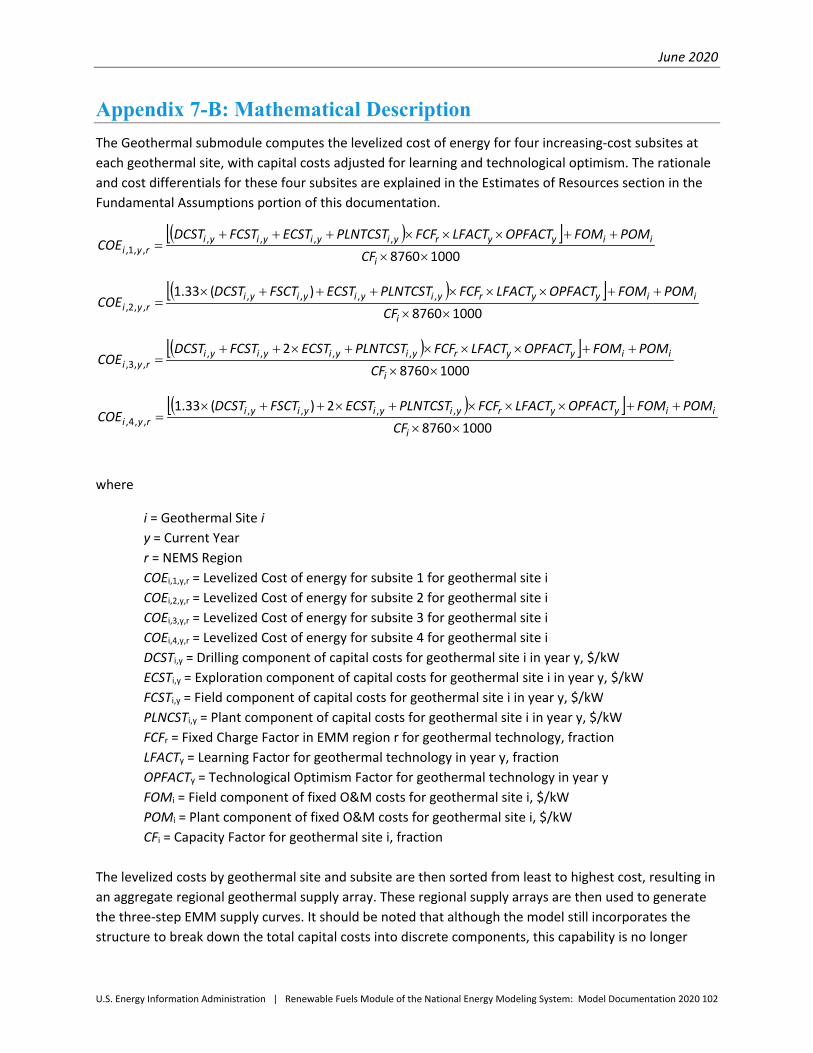
June 2020


Appendix 7-B: Mathematical Description The Geothermal submodule computes the levelized cost of energy for four increasing-cost subsites at each geothermal site, with capital costs adjusted for learning and technological optimism. The rationale and cost differentials for these four subsites are explained in the Estimates of Resources section in the Fundamental Assumptions portion of this documentation.

( )[ ]10008760

,,,,,,1, ××

++×××+++=

i

iiyyryiyiyiyiryi CF

POMFOMOPFACTLFACTFCFPLNTCSTECSTFCSTDCSTCOE

( )[ ]10008760

)(33.1 ,,,,,,2, ××

++×××+++×=

i

iiyyryiyiyiyiryi CF

POMFOMOPFACTLFACTFCFPLNTCSTECSTFSCTDCSTCOE

( )[ ]10008760

2 ,,,,,,3, ××

++×××+×++=

i

iiyyryiyiyiyiryi CF

POMFOMOPFACTLFACTFCFPLNTCSTECSTFCSTDCSTCOE

( )[ ]10008760

2)(33.1 ,,,,,,4, ××

++×××+×++×=

i

iiyyryiyiyiyiryi CF

POMFOMOPFACTLFACTFCFPLNTCSTECSTFSCTDCSTCOE

where

i = Geothermal Site i y = Current Year r = NEMS Region COEi,1,y,r = Levelized Cost of energy for subsite 1 for geothermal site i COEi,2,y,r = Levelized Cost of energy for subsite 2 for geothermal site i COEi,3,y,r = Levelized Cost of energy for subsite 3 for geothermal site i COEi,4,y,r = Levelized Cost of energy for subsite 4 for geothermal site i DCSTi,y = Drilling component of capital costs for geothermal site i in year y, $/kW ECSTi,y = Exploration component of capital costs for geothermal site i in year y, $/kW FCSTi,y = Field component of capital costs for geothermal site i in year y, $/kW PLNCSTi,y = Plant component of capital costs for geothermal site i in year y, $/kW FCFr = Fixed Charge Factor in EMM region r for geothermal technology, fraction LFACTy = Learning Factor for geothermal technology in year y, fraction OPFACTy = Technological Optimism Factor for geothermal technology in year y FOMi = Field component of fixed O&M costs for geothermal site i, $/kW POMi = Plant component of fixed O&M costs for geothermal site i, $/kW CFi = Capacity Factor for geothermal site i, fraction The levelized costs by geothermal site and subsite are then sorted from least to highest cost, resulting in an aggregate regional geothermal supply array. These regional supply arrays are then used to generate the three-step EMM supply curves. It should be noted that although the model still incorporates the structure to break down the total capital costs into discrete components, this capability is no longer

June 2020


used because the data from which EIA gathers its estimates do not have separate cost estimates for each of these categories.

June 2020


Appendix 7-C: Bibliography Augustine, Chad and Young, Katherine. “Updated U.S. Geothermal Supply Curve,” National Renewable Energy Laboratory, February 2010.

California Energy Commission, Public Interest Energy Research, prepared by GeothermEx, “New Geothermal Site Identification and qualification,” April 2004.

California Energy Commission, contract report 500-89-001 prepared by Regional Economic Research, Inc., “Technical Potential of Alternative Technologies, Final Report,” San Diego, CA, December, 1991, Chapter X, “Liquid-Dominated Geothermal Technical Potential.”

Cassel, Thomas A.V.; Edelstein, Robert H.; Blair, Peter D.; Amundsen, Chris B., Technecon Analytic Research, Inc., final report DOE/RA/4713-1 for the U.S. Department of Energy, Assistant Secretary for Resource Application, under contract ET-78-S-02-4713A001 “Geothermal Investment and Policy Analysis With Evaluation of California and Utah Resource Areas,” Philadelphia, PA, October, 1979.

DynCorp I&ET, “Geothermal Supply and Cost Performance Characteristics,” contract deliverable for Purchase Order #36727 for the U.S. Energy Information Administration, Coal and Electric Power Division, Office of Integrated Analysis and Forecasting, June 30, 2000.

Electric Power Research Institute, EPRI TR-106223, prepared by CE Holt Company, project 3657-01, “Next Generation Geothermal Power Plants,” Pasadena, CA, February, 1996.

Entingh, D. and McLarty, L, “Geothermal Cost of Power Model IM-GEO Version 3.05: User’s Manual,” February 22, 1989.

Entingh, Daniel, Princeton Energy Resources, International LLC, under task 9846-004 for the U.S. Department of Energy and National Renewable Energy Laboratory, Working Paper (draft), “Improvements in Geothermal Electric Modeling in the DOE/EIA National Energy Modeling System (NEMS), Volume 2F, Status at Start of May 2000,” Rockville, MD, May, 2000.

Muffler, L.P.J., editor, “Assessment of Geothermal Resources of the United States – 1978,” U.S. Geological Survey Circular 790, 1978.

Northwest Power Planning Council, “Northwest Power in Transition, Opportunities and Risks; Draft Fourth Northwest Conservation and Electric Power Plan,” Portland, OR, March, 1996, Appendix FGT, “Geothermal.”

Petty, Susan; Livesay, B.J; Long, William P.; Geyer, John, Sandia National Laboratory, Contractor Report SAND92-7302 “Supply of Geothermal Power from Hydrothermal Sources: A Study of the Cost of Power in 20 and 40 Years,” Albuquerque, New Mexico, November 1992.

Petty, Susan, Susan Petty Consulting; Livesay, Bill, Livesay Consultants, Inc., prepared for National Renewable Energy Laboratory, “Database of Hydrothermal Sites in the U.S. With Potential for Electric Power Generation,” March, 1993.

June 2020


Western Governors’ Association, “Geothermal Task Force Report: Clean and Diversified energy Initiative,” January 2006.

June 2020



Model name: Geothermal Electric Submodule

Model acronym: GES

Description: The GES projects regional geothermal capacity supplies and cost and performance characteristics used in competing geothermal technologies with fossil, nuclear, and other renewable electricity-generating alternatives for each forecast year and region needing new generating capacity in the EMM. Regional geothermal supplies are based on each region’s share of geothermal resources estimated for 250 identified U.S. geothermal sites, with (1) capital cost estimates for each geothermal site, (2) two-step low-to-high cost estimates of the number of megawatts of capacity available at select site, (3) assumptions for increasing capital costs for increasing portions of the high estimates for each site, and (4) capacity factors, fixed operation and maintenance costs, heat rates, and CO2 emissions rates for each site. Within each region for each model iteration in each forecast year, the GES decrements already chosen resources, arrays all unused geothermal supply in increasing cost order, determines from the EMM the maximum price (avoided cost) likely to be competitive in the EMM, and then provides the EMM three increasing levelized cost-quantity pairs of available capacity in each region for use in competition with other technologies.

Purpose of the model: The purpose of the GES is to provide the Electricity Capacity Planning SubModule (ECP) with the projected amounts of available geothermal generating capacity and its cost and performance characteristics for competition in the ECP for new regional electricity supply in the western United States.

Most recent model update: March 2016

Part of another model: The GES submodule is a component of the Renewable Fuels Module (RFM) of the National Energy Modeling System (NEMS).

Official model representative: Vik Linga Renewable Electricity Analysis Team, Office of Electricity, Coal, Nuclear, and Renewables Analysis U.S. Energy Information Administration, EI-34 1000 Independence Ave., SW Washington, DC 20585

June 2020


Phone: (202) 586-9224 Email: [email protected]

Documentation: This chapter constitutes the documentation of the GES.

Archive media and installation manual: The GES is archived as part of the NEMS production runs.

Energy system described: Hydrothermal geothermal and near-field EGS energy resources of the western United States and the costs and performance characteristics of the technologies converting them to electricity supply.

Coverage: • Geographic: EMM regions 20, 21, 22, 23, and 25. • Time Unit/Frequency: Annual through 2050. • Products: Electricity • Economic Sectors: Electricity Generators

Modeling features: • Modeling Structure: The model operates at the level of individual geothermal sites aggregated to

segmented EMM regional averages. • Model Technique: Levelized electricity costs from each supply segment of each site in each region

are arrayed in increasing cost order, then aggregated into three increasing average-cost segments in each iteration in each year, along with attendant quantities (megawatts) and average heat rates and capacity factors.

• Incorporates short-term cost elasticities of supply, technological optimism, and learning.

Independent expert reviews conducted: None. However, during development of the submodule, ongoing review and comment were obtained from the DOE Office of Energy Efficiency and Renewable Energy, Office of Power Technologies, the National Renewable Energy Laboratory, and from DynCorp Corporation, among others. See Appendix 7-C: Bibliography, above.


June 2020


8. Conventional Hydroelectricity Submodule

Model purpose The Conventional Hydroelectricity Submodule (CHS) represents U.S. conventional hydroelectricity (hydro) resources supply along with each site’s technology cost and performance characteristics used to project new conventional hydroelectric capacity for central station electricity supply through the mid-term future. More specifically, the CHS does the following:

• Provides the Electricity Market Module (EMM) Electricity Capacity Planning (ECP) Submodule the available supply (MW) of new conventional hydroelectric-generating capacity 1 MW or greater (and not more than 10 cents per kilowatthour) as well as its related average cost and performance characteristics based on information about known conventional hydroelectric sites

• Reduces supply available for additional future capacity as conventional hydroelectric capacity resources are used, including capacity identified from historical data, from reported plans, and from resources already chosen in earlier forecasting iterations by the ECP

• Adjusts estimated levelized costs of hydroelectricity from each site based on its public acceptance and the probability of meeting environmental requirements (environmental suitability factor)

• Changes average calculated hydroelectric capital costs, reducing them to reflect experience (learning-by-doing); short-term elasticities are not applied for conventional hydroelectric

• Permits changes in the assumed hydroelectric capital costs for use in alternative cases through the use of capital-cost coefficients by (a) individual site or (b) for all sites in a specific year or multiple years

Identification of sites and costs for use in the CHS was originally estimated by the Idaho National Engineering and Environmental Laboratory from lists assembled from Federal Energy Regulatory Commission license applications and other survey information.20 However, starting with AEO2006, EIA staff eliminated the representation of some large sites found by inquiry to no longer exist and, for retained sites 100 MW or greater, replaced generalized site capacity factors with individual site capacity factors estimated by the Federal Energy Regulatory Commission.

Relationship of the Conventional Hydroelectricity Submodule to Other Models The CHS interacts primarily with the ECP. Relationships between the CHS and other NEMS components include the following:

• CHS provides new capacity availability, performance, and cost information to the ECP for making planning decisions

• CHS uses new capacity build decisions from the ECP to decrement available new conventional resources and capacity

• CHS uses financial parameters and tax data for calculating ECP-based avoided costs to determine the highest cost at which new hydro supply can compete, setting the upper-cost bound of hydro supply

20 Douglas G. Hall, Richard T. Hunt, Kelly S. Reeves, and Greg R. Carroll, Idaho National Engineering and Environmental Laboratory, Estimation of Economic Parameters of U.S. Hydropower Resources INEEL/EXT-03-00662 (Idaho Falls, Idaho, June 2003).

June 2020


Modeling rationale For each NEMS region, the Conventional Hydroelectricity Submodule develops three-part estimates of regional conventional hydroelectric supplies—total MW available in order of three increasing-cost price and quantity pairs. These estimates are used to compete conventional hydroelectric technologies with fossil, nuclear, and other central-station renewable electricity generating alternatives for each forecast year and region needing new generating capacity.

Fundamental assumptions In the underlying hydro resource database, each named hydroelectric site is characterized by its name, location, ownership, resource, cost, and performance characteristics, notably including its (a) components of capital cost, (b) average monthly and annual capacity factors, (c) fixed and variable operating costs, and (d) estimated probability of meeting legal, cultural, and environmental barriers, plus additional identifying information. For each model iteration within each forecast year and region, the CHS arrays all available hydro sites from least to highest cost at or lower than the avoided cost (plus an additional percentage to account for market-sharing, that is, to accept some capacity that is close to competitive) determined in the previous model iteration (an estimate of the upper bound of likely acceptable cost in the current iteration). The CHS then segments the array into three parts—a least-cost, middle-cost, and upper-cost segment—and determines the capacity-weighted average (a) capital cost, (b) operations and maintenance costs, and (c) capacity factors for each group. It then provides the EMM with a conventional hydroelectric supply in the form of three increasing levelized cost-quantity pairs of available hydroelectric capacity.

A significant submodule tool enables the analyst to adjust the CHS to influence forecasts of new hydroelectric capacity by adjusting the proportions of the overall cost range attributed to each segment. A downward adjustment to the proportion of the array (share of the overall range of cost) characterized in the lowest-cost segment, for example, would lower both the average cost of the first segment—thereby increasing the probability of being selected, but relatively decreasing the quantity of capacity likely to be selected. Increasing the proportion of the overall cost range in a segment increases the amount of capacity available in that range but also increases the average capital cost of the capacity as a consequence. Moreover, because each of the three segments characterizes an average, decisions regarding proportions also influence the magnitude of the increase in cost between steps; large proportions can yield large cost increases, and small steps can yield small average increases.

Input data for the supplies were initially provided by the Idaho National Engineering and Environmental Laboratory (INEEL) under a project jointly funded by the U.S. Department of Energy’s Office of Energy Efficiency and Renewable Energy and the U.S. Energy Information Administration.21 The effort is described in Estimation of Economic Parameters of U.S. Hydropower Resources INEEL/EXT-03-00662 (Idaho Falls, Idaho, June 2003). The original database, named IHRED, “Idaho Hydropower Resource Economics Database,” is available through INEEL or EIA as an appendix to the report. The INEEL database, moreover, represents an initial effort in assigning cost attributes to an already-developed site database, the “Hydropower Evaluation Software” (HES) database, based on (1) The Federal Energy

21 Contract DE-AC007-99ID13727, completed June, 2003.

June 2020


Regulatory Commission’s Hydropower Resource Assessment database developed from hydropower licensing actions, (2) the Nationwide Rivers Inventory Database developed and maintained by the National Park Service, and (3) supporting information from state resource and energy agencies.22 The more recent INEEL IHRED effort supplemented the HES by providing generalized estimates of capital and other costs, as well as generalized (regional) estimates of capacity factors. Costs and other monetary values in IHRED are expressed in 2002 dollars (NEMS expresses these same values in 1987 dollars).

For AEO2006 and subsequent reports, EIA modified the IHRED in the following ways. First, HES-estimated capacity factors specific to each hydro site replaced the regional generalized estimates from IHRE. In general, the site-specific estimated capacity factors are lower than the IHRED factors but are considered superior, based on specific assessments of the sites. Second, to reduce workload, EIA eliminated from consideration all sites for which an off-line estimate of the levelized cost of generation exceeded 10 cents per kilowatthour (2002 dollars), given the near impossibility of any such site being selected in any conceivable scenario. Third, the IHRED database was separated into two groups, small sites (100 MW or less) and large sites (greater than 100 MW). Data on all small sites were accepted for use. Finally, large sites were arrayed from least to highest cost and then individually reviewed, to the extent permitted by time and resources, contacting site owners or state agencies to verify the existence and viability of such sites. Many large sites were found unavailable (already developed, otherwise developed, now precluded by Wild and Scenic Rivers, or other circumstance making development naturally or legally impossible). Not all large sites were examined. Documentation of calculations and modifications can be found in the EIA-maintained Excel files HydroLessThan10cents033004.xls and HydroCritiqueTop100041904.xls.

Resources The CHS characterizes economic supply of both run-of-river and storage dams for conventional hydroelectric power at new or existing sites 1 MW or greater. The model incorporates data on some—although not all—potential hydroelectricity supply, including undeveloped sites with no dam, opportunities for adding hydroelectric capacity at existing dams without hydropower, and opportunities to increase capacity at existing hydroelectric facilities.

Exclusions The CHS does not represent all hydroelectric potential. First, the CHS does not represent opportunities less than 1 MW capacity. Second, the CHS does not enumerate new pumped storage hydroelectricity potential, an energy storage technology using off-peak coal or nuclear-powered electricity to lift water to an upper pool for later peaking hydro generation (operation of existing pumped storage, however, is modeled in the EMM.) Third, the supply also omits sites excluded from development by federal statutes and policies, including hydro resources excluded by the Wild and Scenic Rivers Act (or sited at the upstream or downstream ends of wild and scenic streams or on a tributary, in National Parks, or otherwise excluded by federal or state law or in a federally designated exclusion zone). Furthermore, the CHS does not represent offshore (ocean) hydro, in-stream (non-impoundment) potential, additional potential from refurbishing existing hydro capacity, or increased output opportunities from efficiency or

22 Alison M. Conner, James E. Francfort, and Ben N. Rinehart, Idaho National Engineering and Environmental Laboratory, U.S. Hydropower Resource Assessment, Final Report, Contract DE-AC07-94ID13223 (Idaho Falls, Idaho, December 1998).

June 2020


operational improvements, any or all of which could also add to U.S. hydroelectric supply. In addition, the CHS does not represent any sites for which off-line EIA estimates made in 2004 indicated levelized per-kilowatthour costs (in 2002 dollars) greater than 10 cents per kilowatthour. EIA staff also eliminated from the supply a number of sites 100 MW or greater that, based on contacts with owning firms, were concluded to not be available today—with the identified resources already developed, excluded from development by law, or otherwise unable to offer additional potential today. Finally, the CHS does not account for any unknown additional conventional hydroelectric potential that might become available at known sites included in these estimates.

Capital costs Overnight capital costs—and all other costs—are expressed in 2002 dollars. Components of overnight capital costs include licensing, construction, and a range of individual environmental mitigation costs (see below) as applicable to individual sites. Construction costs include land and rights, structures and improvements, reservoirs, dams, waterways, equipment, and access roads, rail, and bridges. Construction costs were derived by INEEL primarily from 1990–2000 FERC Form 1, Annual Report of Major Electric Utilities, Licensees, and Others.

Learning by doing Learning by doing refers to reductions in a technology’s capital costs as experience with the technology is gained, expressed in NEMS as a function of the total amount of capacity in place. Therefore, the capital costs of conventional hydroelectric plants decrease in NEMS as additional capacity is built.

For a description of learning by doing in NEMS, see either Electricity Market Module Assumptions for the Annual Energy Outlook or Electricity Market Module of the National Energy Modeling System, Model Documentation Report for the relevant Outlook year. Conventional hydroelectricity is considered a mature technology, meaning that hydroelectricity is already well developed and that capital costs will likely decrease at the slowest rate.

NEMS also includes a minimum decrease in capital costs independent of actual builds.

Short-term elasticities In NEMS, capital costs for most technologies are assumed to increase if capacity increases rapidly within a given year, thereby temporarily squeezing supply resources (such as skilled labor, materials, and manufacturing). More information for these elasticities can also be found in the Assumptions and Documentation reports. These short-term elasticities are not applied to conventional hydroelectricity, because U.S. and global infrastructure are currently considered fully capable of meeting all demand for the mature technology.

Mitigation costs—construction component For sites not prohibited from development but nevertheless facing environmental mitigation requirements, the construction costs of such mitigation are individually estimated and included among capital costs derived from a variety of sources documented in the INEEL report. Individual categories of potential mitigation cost include archeological requirements, fish and wildlife protection, scenic or recreation requirements, water quality monitoring, and fish passage requirements. All are expressed in 2002 dollars per kilowatt and are included among capital costs.

https://www.eia.gov/outlooks/aeo/assumptions/pdf/electricity.pdf

https://www.eia.gov/outlooks/aeo/assumptions/pdf/electricity.pdf

June 2020


Mitigation costs—public acceptance component IHRED-estimated mitigation costs account for the bricks and mortar construction costs of mitigation requirements. To account for the litigation, licensing, and public acceptance costs of mitigation, EIA adapted the HES environmental suitability factor to estimate the probability of a hydroelectric project’s successful development in light of all individual environmental characteristics of the site. Suitability factors range from 0.90 (the greatest probability of meeting environmental requirements and being developed), through 0.75, 0.50, 0.25, and finally, 0.10. The HES included no estimates of the costs of overcoming likely objections. However, EIA incorporated into its submodule an arbitrary estimate of levelized additional costs per kilowatthour to represent the added costs of meeting environmental requirements—legal challenges, studies, and public outreach—in addition to the engineering costs already accounted:

If Site Probability = 0.90, then add 0.00 mills to levelized cost (1987$) If Site Probability = 0.75, then add 3.00 mills to levelized cost (1987$) If Site Probability = 0.50, then add 5.00 mills to levelized cost (1987$) If Site Probability = 0.25, then add 8.00 mills to levelized cost (1987$) If Site Probability = 0.10, then add 10.00 mills to levelized cost (1987$)

These cost adjustments almost certainly eliminate most of the 0.25 and 0.10 probability sites from practical consideration and greatly reduce the competitive potential of 0.50 sites as well. Changing the costs associated with site probabilities offers another opportunity for analyst influence on hydroelectric supply costs.

Fixed operation and maintenance costs Fixed Operation and Maintenance (O&M) costs include operation and maintenance supervision and engineering, as well as maintenance of structures, reservoirs, dams, waterways, and electric plants; where applicable, fixed O&M includes the Federal Energy Regulatory Commission (FERC) annual charge noted below. Fixed O&M costs were derived from FERC Form 1 data for 1990 to 2001 and are expressed in 2002 dollars per kilowatt per year.

FERC annual charge For plants with a capacity greater than 1.5 MW, FERC charges plant owners an annual fee based on plant capacity and annual generation. The FERC annual charge is considered part of fixed O&M and is estimated using an estimate of constant annual generation derived by INEEL, based on 1999 charges.

Variable operation and maintenance costs Variable O&M maintenance costs, also derived from FERC Form 1 data, include estimates for charges for water for power, hydraulic and electric expenses, miscellaneous hydraulic power expenses, and rents. Variable O&M is expressed in 2002$ mills per kilowatthour.

Capacity factors The IHRED database contains both estimated monthly and annual capacity factors for each site. However, EIA replaced these regional average annual capacity factors with the individually determined annual capacity factors established by FERC or in other specific studies underlying the HES database; monthly IHRED capacity factors were then modified in proportion to the annual factor adjustment. In

June 2020


general, the individual capacity factors are lower than the generalized estimates. Moreover, EIA also applied exceptions, and it used the IHRED estimate or 65% (whichever was lower) for undeveloped sites for which no FERC capacity factor was available and 35% for incremental capacity for which no FERC capacity factor was available. Where the FERC capacity factor exceeded 65% for new sites or 35% for incremental capacity, EIA assigned either 65% or 35%, given that the EIA bound, although arbitrary, is higher than the averages for known sites, and the FERC values appear to often be in error (at times exceeding 100%).

Regional adjustment factors are used in the CHS to enable modification of projected hydroelectric output on a regional level. This adjustment may be necessary for years where projected hydroelectric generation is anomalously high or low. Current regional adjustment factors are set so that the result of multiplying them by the site-specific capacity factors approaches a 20-year average.

Heat rates Conventional hydroelectric facilities tend to be highly efficient; the Federal Energy Regulatory Commission cites modern hydroelectric turbines to be about 90% efficient (90% of input energy converted to output electricity), suggesting an average input heat rate equivalent under 3800 Btu per kilowatthour.23 EIA has adopted a convention of using the average heat rate for fossil-fueled generators to represent the primary energy consumption of all renewable generation sources that do not require the combustion of a fuel, including hydroelectric. This convention is currently set at the heat rate for fossil-fueled steam-electric plants of 9,756 Btu per kilowatthour.24

Alternative approaches Before developing the Conventional Hydroelectric Submodule, EIA staff extensively polled hydroelectricity analysts and organizations and conducted ongoing exchanges with contacts at the National Hydropower Association, Oak Ridge National Laboratory, the Bonneville Power Administration, the Tennessee Valley Authority, and others. Although many annual and short-term regional forecasting models of expected output from existing hydroelectric capacity can be found, no models of mid- or longer-term hydroelectric supply were found, either of resources expressed in terms of economic supply or in terms of their competition with other central station electricity supplies.

Conventional Hydroelectric Submodule structure The CHS SUBROUTINE HYDRO has five basic components:

1. Incorporates data: On its initial iteration, subroutine GET_HYSITE_DATA reads the hydroelectric site data from the HYDSITE.TXT input data file containing records of each individual hydroelectric site, including state and NEMS region, nameplate capacity, capital and O&M cost components, and capacity factors. Subroutine GET_HYDATA reads in the annual capital cost multipliers, build-bounds, public acceptance mitigation costs, and the supply curve cost segment ranges from the input data file WHYDRO.TXT. Together the two build the HYDSITE conventional hydroelectric supply structure.

23 Federal Energy Regulatory Commission, Hydroelectric Power Resources of the United States, Developed and Undeveloped (Washington, DC January 1, 1992), page xx. Applying the 90% efficiency cited by FERC to the 3412-Btu-per-kilowatthour energy content of electricity yields an input heat rate of 3,791 input Btu per kilowatthour. 24 See Table A6 at http://www.eia.gov/totalenergy/data/annual/#appendices .

http://www.eia.gov/totalenergy/data/annual/#appendices

June 2020


Capital costs are the sum of licensing, construction, and environmental mitigation costs; both fixed and variable O&M costs are incorporated; hydroelectricity has no fuel charges, although the FERC annual charge is included, where applicable, with fixed O&M. The annual capital cost multipliers are applied to the capital costs before leaving the GET_HYSITE_DATA subroutine. The cost multipliers will usually have the value 1.00 for reference cases and various values less than 1.00 for alternative scenarios such as high renewables cases.

2. Develops NEMS overall regional conventional hydroelectric supplies: In each iteration, subroutine BLD_HYD_CURVES first creates NEMS regional conventional supplies for each NEMS region (Alaska and Hawaii are processed in the hydroelectric submodule but not used by the EMM). Within each NEMS region, sites are arrayed from least to greatest in order of estimated levelized cost, resulting in an aggregate conventional hydroelectric supply for each region in each iteration, in the array HYDCURVE.

3. Provides sub-supplies for specific regional demands: For each iteration of the EMM, the CHS determines the maximum levelized cost (avoided cost) at which hydroelectric supply in each region can compete. The maximum competitive value is (1) the levelized cost of the highest-cost technology actually selected in the immediately previous iteration of the ECP plus (2) an additional percentage representing the market-sharing algorithm.25 As a result, all remaining hydroelectric capacity able to generate at or lower than the previous iteration’s maximum competitive value is offered as new hydroelectric supply in the current iteration. Next the subroutine BUILD_HYD_CURVES segments each region’s aggregate hydroelectric supply among three increasing-cost quantity pairs using capacity-weighted average costs per kilowatthour. This segmentation provides the EMM three quantities of available conventional hydroelectric capacity, as well as their respective O&M costs and seasonal and annual capacity factors at three increasing levelized costs for each region. The gross cost difference between the least-cost unused hydroelectric capacity and the ECP-adjusted avoided cost is used to identify the three groups. The least-cost group includes all unused capacity in the least-cost quartile (capacity whose levelized cost is equal to or less than +25% of the gross cost difference). It is important to note that the quantity in this group is not the least-cost 25% of capacity, but instead whatever proportion of capacity occurs in the lowest 25% of the cost range. The second group includes all capacity between the 25th percentile and the 75th percentile; and the third group includes all remaining capacity higher than the 75th cost percentile. All available capacity in each cost group is then conveyed to the EMM as available supply, with one levelized cost associated with each group. The one levelized cost transmitted for each group equals the capacity-weighted levelized average cost for the individual sites’ costs within the group. A model variable enables the analyst to vary the initial percentage thresholds. The consequence of lower thresholds is lower average costs—and greater ability to compete—but reduced quantities available to compete, whereas higher thresholds yield greater supplies but higher (and less-competitive) average costs. Recognizing that the three segments yield significant increases in average costs (discontinuities) from one step to the next, the choice of

25 The market-sharing algorithm exists in recognition that in real markets technologies that are close in cost to the least-cost technology will occasionally be selected for economic and other reasons not represented in the modeling. Under the sharing algorithm, the closer in cost a specific other technology is to the least-cost technology, the greater (yet small) share of the available market will be taken by that technology.

June 2020


thresholds can result in significant differences in NEMS selections of conventional hydroelectric capacity, particularly if choices have the effect of limiting supply to one (or none) of the segments.

4. Decrements available capacity: Within subroutine BUILD_HYD_CURVES, for each iteration, CHS reduces available conventional hydroelectric capacity in each region in response to (a) external reports of new hydroelectric builds in the region or (b) selection by the EMM in earlier iterations.

5. Provides diagnostics: For each iteration, subroutine WRITE-HYDB provides diagnostic information on hydroelectric capacity, sites chosen, technology costs, and performance. Diagnostics provided through Excel output file HYDRO_OUT.XLS include the following datasets:

Hyd_Input_Data displaying quantities of capacity available at each hydroelectric site;

Hyd_Curve_Data displaying in least-to-highest cost order each hydroelectric site’s capacity and estimated cost per kilowatthour;

Hyd_Curve_Info displaying aggregate conventional hydro supplies and average cost per kilowatthour as available in each NEMS region for each forecast year, values transmitted to the Electricity Market Module (EMM) as aggregate hydroelectric supply; and

Hyd_Builds displaying quantities of conventional capacity built in each NEMS region in each forecast year.

Key computations and equations This section describes the most important equations in the CHS.

Reading the data In the first iteration, data for the hydroelectric sites are read in from the HYDSITE input file by the CHS subroutine, GET_HYSITE_DATA. The site data are stored in the HYDSITE data structure, which is defined below. Subroutine GET_HYDATA reads the hydro parameters from the input file WHYDRO.

HYDSITE Data Structure:

PROJNAME Project Name PROJNUM Project Number STATE State Location SITE_ID Site ID NERC EMM Region LATITUDE Latitude LONGITUDE Longitude CLASS Site Class Code: C=Coop, F=Federal, I=Industrial, M=Municipal, P=Private Utility, R=Private Non-Utility, N/A=Not Available UNITTYPE C=Conventional, R=Reversible, Z=Missing PLNTTYPE Plant Type PROJSTATUS Project Status DAMSTATUS Dam Status WSPROT Wild/Scenic Protection Y=Yes, N=No

June 2020


WSTRIB Wild/Scenic Tributary, Location Y=Yes, N=No ENVVALUES Environmental Values, Y=Yes, N=No 1=Cultural Value, 2=Fish, 3=Geological, 4=Historical, 5=Other, for example, rare wetland, wilderness designation, 6=Recreation 7=Scenic, 8=Wildlife, 9=Threatened/Endangered Wildlife 10=Threatened/Endangered Fish LANDCODES Federal Land Codes, Y=Yes, N=No 1=FLC103, National Park, Monument, Rec area, etc., 2=FLC104, National Forest or Grassland, 3=FLC105, National Wildlife Refuge, Game Preserve, or Fish Hatchery 4=FLC106, National Scenic Waterway or Wilderness Area 5=FLC107, Indian Reservation 6=FLC108, Military Reservation 7=FLC198, Not on Federal Land SITEPROB Project Environmental Suitability Factor 0.10 = Development prohibited or highly unlikely 0.25 = Major reduction in likelihood of development 0.50 = Likelihood of development reduced by half 0.75 = Minor reduction in likelihood of development 0.90 = Little effect on likelihood of development LISCCOST Licensing Cost 2002 $K CONSCOST Construction Cost 2002 $K DEVCOST Overnight Development Cost 2002 $K MIT_ARCH 30-Year Archaeological and Historical mitigation cost 2002 $K MIT_FISH 30-Year Fish and Wildlife mitigation cost 2002 $K MIT_SCEN 30-Year Scenic and Recreation mitigation cost 2002 $K MIT_WATER 30-Year Water Quality Monitoring Cost 2002 $K MIT_PASS 30-Year Fish Passage cost 2002 $K MIT_TOTAL Total mitigation cost 2002 $K TOTDEV_COST Total Development Costs (Mit_Total + Devcost) 2002 $K UNITDEV_COST Total Unit Development Costs 2002$/kW COE Levelized Cost 2002$/MWh CAP_COST Capital Cost 2002$/kW TOTFOM_COST Average Annual Fixed O&M Cost 2002 $K TOTVOM_COST Average Annual Variable O&M Cost 2002 $K FOM_COST Average Annual Fixed O&M Unit Cost 2002$/kW VOM_COST Average Annual Variable O&M Unit Cost 2002$/MWh FERC_COST FERC Annual Charge (Applicable if >= 1.5 MW) 2002 $K UNITFERC_COST FERC Annual Charge Unit Cost (Applicable if >= 1.5 MW) 2002$/KW POTENTIAL_CAP Potential Capacity (MW) CAPCOST_MULT Yearly Capital Cost Multipliers by Hydro Sites CAP_COST_ADJ Capital Cost Adjustment Factors

June 2020


MON_CAPACITY_FACTOR(12) 0.00 TO 1.00 - monthly capacity factors AVG_CAPACITY_FACTOR 0.00 TO 1.00 - average annual capacity factors

In each iteration, the capital, O&M, and levelized cost of energy for each site is calculated, and capital costs are adjusted for learning and technological optimism. Technological optimism and learning effects are estimated in subroutine ELEC_OPT in the Electricity Capacity Planning (ECP) Submodule of the EMM.

Building regional hydroelectric supplies In each iteration, data on supplies at each site are merged with cost data from other sites in each region and arrayed for competition in the ECP within the region. The CHS first constructs a hydroelectric supply curve of levelized cost of energy and capacity available for each EMM region. CHS then segments the competitive part of that array into three generalized increasing cost segments (as described in the Conventional Hydroelectric Submodule Structure section), passing to the ECP the total capacity available in each increasing cost segment along with the capacity-weighted cost and performance parameters for the segment.

For each region and in each iteration, the CHS receives a maximum cost from the EMM, a value equal to the COE of the highest cost capacity previously selected in each region, called the Regional Avoided Cost, plus the market-sharing tolerance. This avoided cost is used to determine the competitive part of the arrayed costs.

Avoided Cost = (Regional Maximum Prior COE) * (1.0 + Market-sharing Tolerance)

The subroutine BUILD_HYD_CURVES iterates within each region until the capacity available in the first (lowest-cost) step is greater than zero or 10 iterations have occurred, incrementing the threshold cost 10% for each iteration. The cumulative values calculated in this subroutine include the following:

AVAIL_SUPPLY = Megawatts available for each record CUM_SUPPLY = Cumulative sum available megawatts in each region SYS_CAP_COST = Cumulative capacity-weighted capital cost, three segments SYS_CAP_FAC = Cumulative capacity-weighted capacity factor, three segments SYS_MON_CAP_FAC = Cumulative capacity-weighted monthly capacity factors, three segments SYS_COST = Cumulative capacity-weighted COE, three segments SYS_VOM_COST = Cumulative capacity-weighted Variable O&M cost, three segments SYS_FOM_COST = Cumulative capacity-weighted Fixed O&M cost, three segments

From these cumulative values BUILD_HYD_CURVES then determines the specific value for the cost and performance variables for each of the three segments of available hydroelectric supply in each region. The cost and performance variables calculated include the following:

CAP_COST = Capital cost CAP_FAC = Capacity factor MON_CAP_FAC = Monthly capacity factors FOM_COST = Fixed O&M cost VOM_COST = Variable O&M cost

June 2020


The above values are calculated as weighted averages as shown in the equations below, where i represents each individual site:

Average_Capital_Cost = (∑i (CAP_COST(i) * Capacity(i) ))/ Cumulative_Capacity Average_FOM_Cost = (∑i (FOM_COST(i) * Capacity(i) ))/ Cumulative_Capacity Average_VOM_Cost = (∑i (VOM_COST(i) * Capacity(i) ))/ Cumulative_Capacity Average_Cap Fac = (∑i (CAP_FAC(i) * Capacity(i) ))/ Cumulative_Capacity Average_Mon_Cap Fac = (∑i (MON_CAP_FAC(i) * Capacity(i) ))/ Cumulative_Capacity

The CHS passes the ECP actual values only for the first of the three segments; values for steps 2 and 3 are expressed as weights applicable to the values in the first segment. The variables passed to the EMM include the following:

EMM_CAP_COST EMM_CAP_FAC EMM_MON_CAP_FAC EMM_CAPACITY EMM_VOM_COST EMM_FOM_COST

Other features of the Hydroelectric Submodule Construction Lead Time, Construction Cost Profile, and First Online Year: In the CHS, new hydroelectric plants are constructed over a four-year time period, and capital costs are allocated in the annual proportions 15%, 22%, 30%, and 33%.

Learning, Short-Term Elasticities, and Technological Optimism: Capital Costs for hydroelectric-generating technologies are affected by learning-by-doing (as are all generating technologies), as well as by technological optimism. For a description of these characteristics and assumptions and values used for hydroelectric, see Assumptions to the Annual Energy Outlook 2020: Electricity Market Module.

June 2020


Appendix 8-A: Inventory of Variables, Data, and Parameters Values for this inventory are included in the body of this chapter, along with reference to the Excel files supporting the Conventional Hydroelectricity Submodule. Questions about the submodule can be directed to the Official Model Representative, listed in Appendix 8-D. Data files for the CHS are maintained in the Office of Electricity, Coal, Nuclear, and Renewables Analysis (OECNRA). The INEEL deliverable is also available through OECNRA.

June 2020


Appendix 8-B: Mathematical Description Questions about the CHS algorithm can be directed to the Official Model Representative, listed in Appendix 8-D. The Conventional Hydroelectricity Submodule computes the levelized cost of energy for three increasing cost segments of conventional hydroelectric supply in each NEMS region in each NEMS iteration for each forecast year. Rationales are explained in the Model Purpose and Fundamental Assumptions portion of this documentation. The levelized cost for each site is calculated as follows:

( )ii

i

iiyyryiyiyiryi PUBCOSTVOM

CFFERCFOMOPFACTLFACTFCFMCSTLCSTCCST

COE ++××

++×××++=

10008760,,,

,,

where

i = Hydroelectric Site y = Current Year r = NEMS Region COEi = Levelized cost of energy for hydroelectric site i. CCSTi,y = Construction costs for hydroelectric site i in year y, $/kW. LCSTi,y = Licensing costs for hydroelectric site i in year y, $/kW. MCSTi,y = Total mitigation costs for hydroelectric site i in year y, $/kW. FCFr = Fixed Charge Factor in EMM region r for hydroelectric technology, fraction. LFACTy = Learning Factor for hydroelectric technology in year y, fraction. OPFACTy = Technological Optimism Factor for hydroelectric technology in year y, fraction.

FOMi = Fixed O&M costs for hydroelectric site i, $/kW. FERCi = FERC Annual Charge for hydroelectric site i, 1987 $/kW. CFi = Capacity Factor for hydroelectric site i, fraction. VOMi = Variable O&M costs for hydroelectric site i, $/MWh. PUBCOSTi = Public Acceptance Cost for hydroelectric site i, $/MWh.

The levelized costs by hydroelectric site are then sorted from least to highest cost, resulting in an aggregate regional hydroelectric supply array. These regional supply arrays are then used to generate the three-step EMM supply curves.

June 2020


Appendix 8-C: Bibliography Conner, Alison M. , Francfort, James E., and Rinehart, Ben N., Idaho National Engineering and Environmental Laboratory, U.S. Hydropower Resource Assessment, Final Report, Contract DE-AC07-94ID13223 (Idaho Falls, ID, December 1998).

Federal Energy Regulatory Commission, Hydroelectric Power Resources of the United States, Developed and Undeveloped (Washington, DC, January 1, 1992).

Hall, Douglas G., Hunt, Richard T., Reeves, Kelly S., and Carroll, Greg R., Idaho National Engineering and Environmental Laboratory, Estimation of Economic Parameters of U.S. Hydropower Resources INEEL/EXT-03-00662 (Idaho Falls, ID, June 2003).

June 2020



Model name: Conventional Hydroelectricity Submodule

Model acronym: CHS

Description: The CHS converts lists of identified available U.S. conventional hydroelectric potential and costs into three-part increasing-cost regional supply projections (quantity-cost pairs) for each NEMS region for each forecast year. Input data for each site include its state and NEMS region, components of capital cost, fixed and variable operations and maintenance costs, and capacity factors. All sites able to produce electricity at or lower than an avoided cost determined by NEMS in the previous forecast cycle (adjusted upward for market-sharing) become eligible to compete as new hydroelectric supply averaged among one of the three increasing cost groups. After selecting some capacity, the CHS decrements the available supply for the next iteration by the amount taken in the current cycle.

Purpose of the model: The purpose of the CHS is to provide the Electricity Capacity Planning (ECP) module the amounts of available conventional hydroelectric-generating capacity, their costs, and performance characteristics for competition in the ECP for new regional electricity supply.


Part of another model: The CHS submodule is a component of the Renewable Fuels Module (RFM) of the National Energy Modeling System (NEMS).

Official model representative: Michelle Bowman Renewable Electricity Analysis Team, Office of Electricity, Coal, Nuclear, and Renewables Analysis U.S. Energy Information Administration, EI-34 1000 Independence Ave., SW Washington, DC 20585 Phone: (202) 586-0526 Email: [email protected]

Documentation: This chapter constitutes the documentation of the CHS.

June 2020


Archive media and installation manual: The CHS is archived as part of NEMS production runs.

Energy system described: Conventional hydroelectric supply includes potential 1 megawatt or greater for impoundment sites (a) undeveloped, (b) with dams but no hydroelectric, or (c) with potential for additional hydroelectric. The supply does not include pumped storage opportunities, in-stream (non-impoundment) potential, ocean-current potential, or refurbishments of existing capacity or operational changes that increase output.

Coverage: • Geographic: 25 EMM regions (Note: Alaska and Hawaii are included in the database and processed

in the submodule, but they are excluded from the EMM) • Time Unit/Frequency: Annual through 2050 • Products: Electricity • Economic Sectors: Central Station Electricity Generators

Modeling features: • Modeling Structure: The model operates at the level of individual conventional hydroelectric sites

aggregated to segment-level EMM regional averages. • Model Technique: Levelized electricity costs of each site in each region are arrayed in increasing

cost order, then aggregated into three increasing average-cost segments in each iteration in each year, along with corresponding capacity quantities (megawatts), average heat rates, and capacity factors.

• Incorporates short-term cost elasticities of supply, technological optimism, and learning.

Input sources: The primary data input for the conventional hydroelectricity supply is a dataset prepared specifically to support the modeling. The dataset is prepared under contract by the Idaho National Engineering and Environmental Laboratory. The INEEL contract work integrated data published by Hall, Douglas G., Hunt, Richard T., Reeves, Kelly S., and Carroll, Greg R., (INEEL) in Estimation of Economic Parameters of U.S. Hydropower Resources INEEL/EXT-03-00662 (Idaho Falls, Idaho, June 2003), along with information from other documents cited in Appendix 8-C.

Independent expert reviews conducted: None. However, the CHS methodology was presented at a May 10, 2005, Renewable Electricity Modeling Forum with the specific purpose of exposing the submodule to independent expert review.


renewable fuels module of the national energy modeling

Documents