renewable asset risk management
TRANSCRIPT

Manuele Monti, Ph.D.GDF Suez Energia Italia Energy Management - Power & Risk Portfolio
Renewable asset risk management for fixed price offers
Presentation Title
Mercati energetici e metodi quantitativi: un ponte tra Università e Aziende
22-23 Maggio, Padova
E' vietata la riproduzione , e ridistribuzione sotto ogni forma, anche parziale, di immagini, testi o contenuti senza autorizzazione dell’autore e di GDF Suez Energia Italia S.p.A.Le indicazioni modellistiche, le conclusioni, i prodotti strutturati mostrati sono proprietà industriale di GDF Suez. I riferimenti allo sviluppo quantitativo, all’open innovation e alle reti di conoscenza rappresentano libera ed individuale espressione intellettuale dell’autore.Copyright all contenents reserved. For English conditions and disclaimer disclaimer please contactthe author.
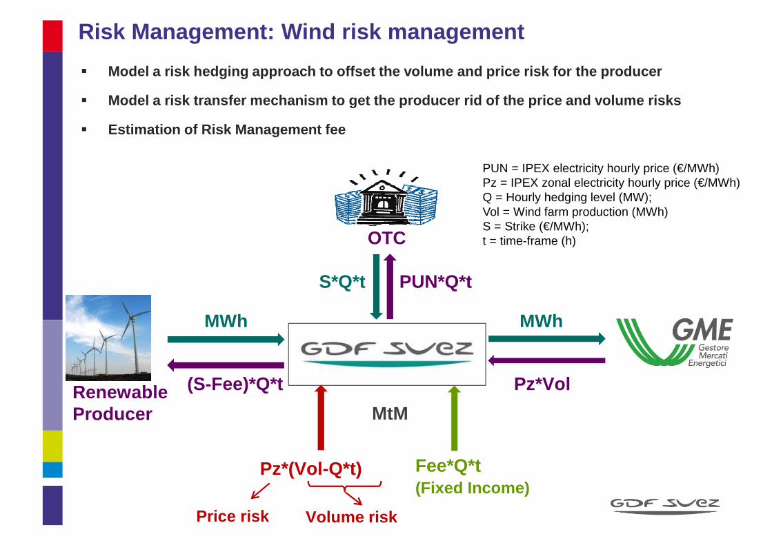
� Model a risk hedging approach to offset the volume and price risk for the producer
� Model a risk transfer mechanism to get the producer rid of the price and volume risks
� Estimation of Risk Management fee
MWh
(S-Fee)*Q*t
MWh
Pz*Vol
S*Q*t PUN*Q*t
RenewableProducer
OTC
PUN = IPEX electricity hourly price (€/MWh)Pz = IPEX zonal electricity hourly price (€/MWh)Q = Hourly hedging level (MW);Vol = Wind farm production (MWh)S = Strike (€/MWh);t = time-frame (h)
Pz*(Vol-Q*t) Fee*Q*t(Fixed Income)
Price risk Volume risk
MtM
Risk Management: Wind risk management
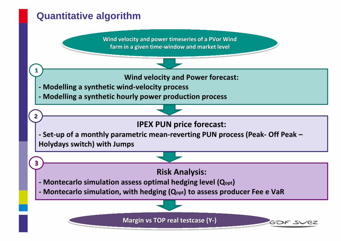
Margin vs TOP real testcase (Y-)
Wind velocity and power timeseries of a PVor Wind
farm in a given time-window and market level
Wind velocity and Power forecast:
- Modelling a synthetic wind-velocity process
- Modelling a synthetic hourly power production process
1
Risk Analysis:- Montecarlo simulation assess optimal hedging level (Qopt)
- Montecarlo simulation, with hedging (Qopt) to assess producer Fee e VaR
3
IPEX PUN price forecast:- Set-up of a monthly parametric mean-reverting PUN process (Peak- Off Peak –
Holydays switch) with Jumps
2
Quantitative algorithm

0 5 10 15 20 25 300
200
400
600
800Wind velocity (V)
[m/s]
Nsa
mpl
es
0 10 20 30 40 50 60 70
500
1000
1500Power output (Pout)
[MW]
V Cut-Off
λexp; kexp
Wind velocity and Power forecast:
- Modelling a synthetic wind-velocity process
- Modelling a synthetic hourly power production process
1
Wind modelization
From the experimentally revealed V/P
timeseries a Weibull distribution is
parametrized by the mean of a Maximum
Likelyhood method; ����λexp; kexp .
1a

The synthetic power process is obtained by
convolution of the wind process through
the wind-power curve. -10 0 10 20 30 40 50 60 70 800
200
400
600
800
1000
1200
1400
1600
[MW]
Oss
erva
zio
ni s
ul p
roce
sso
Potenza
Synthetic: power
Synthetic: wind
Experimental
A simulation of the synthetic velocity
distribution with given Weibull parameters
is thereafter obtained.
The farm wind velocity-energy production
curve is modelled by a polynomial
regression on the experimental power load
From the experimentally revealed V/P
timeseries a Weibull distribution is
parametrized by the mean of a Maximum
Likelyhood method; ����λexp; kexp .
1b
Wind asset modelization
1a
Wind velocity and Power forecast:
- Modelling a synthetic wind-velocity process
- Modelling a synthetic hourly power production process
1

PV power plant assessment
2 4 6 8 10 12 14 16 18 20 22 240
1
2
3
4
5
6
Hour
Pow
er [
MW
]
Jan
FebMar
Apr
May
JunJul
Aug
Sep
OctNov
Dic
A preliminary assessment on the PV plant average daily profile was performed for each month of the year, based on the historical data of the plant from May 2011 to Dec 2013.
The results are plotted in the figure above.
Plant data Description
Installed power [kW] 7775,48
Expected yearly prodction [kWh]10.574.000
Power module unit [W]255
Efficiency module [%]
Number of modules30492
Tilt [ ° ]30
Direction [ ° ]0
Surface [m2]150.000
Latitude40°22' 14''
Longitude18° 06' 07''
Total efficiency* [%]82
* This accounts for all the losses up to the immission point

PV power plant assessment
2 4 6 8 10 12 14 16 18 20 22 240
1
2
3
4
5Yearly average production PK hedge
hour
Pow
er [
MW
]
2 4 6 8 10 12 14 16 18 20 22 24-2
0
2
4
hour
Pow
er [
MW
]
Residual exposure
Production
Hedge
The idea is to hedge the expected production forecast profile with a standard OTC PK Calendar product, and bear the residual exposure in the EM portfolio.The deterministic production of a PV power plant determines a long position in the central hours (h 11-18) and a short position in the peripheral hours (8-11 and 18-21)
This residual short exposure matches the double peaks of the PUN prices (residual demand covered by conventional power generation). This generates a negative exposure in the EM portfolio (around 30% of the total production).
Short
Short
Long
+
--
+LongShort
-Short
-

PUN stress Callisto scenario
0 1000 2000 3000 4000 5000 6000 7000 8000 90000
50
100
150
200
250
300
350
hour
Pric
e [€
/MW
h]
Product [€/MWh] Q_01 Q_02 Q_03 Q_04 Mean
PW_IT_BS 70,3 67,9 72,2 71,2 70,4
PW_IT_OF 64,2 65,5 69,2 65,8 66,2
PW_IT_PK 81,4 72,3 77,5 80,8 78,0
The power price scenario was stressed by using 1000 scenarios generated by Callisto tool:
• Reference date: 31/12/2012• Simulation window: 01/01/2013 –
31/12/2013• Hourly granularity
The scenarios generated match as an averagethe FWD quarterly prices, and the intraday hourly shape realized on the learning period of the model (01/01/2012 – 31/12/2012)

Multivariate Ornstein–Uhlenbeck process with Jumps:
= deterministic mean-reverting transition matrix
= unconditional expectation vector (based on historical and FWD screen prices)
= dispersion square matrix (namely scatter generator, historical prices only)
= vector of independent Wiener processes
= UOL multivariate processes vector
= Jump regimes vector (from seasonal statistics and hybrid physical market models)
IPEX PUN price forecast:- Set-up of a monthly parametric mean-reverting PUN process (Peak- Off Peak – Holydays switch) with Jumps
2
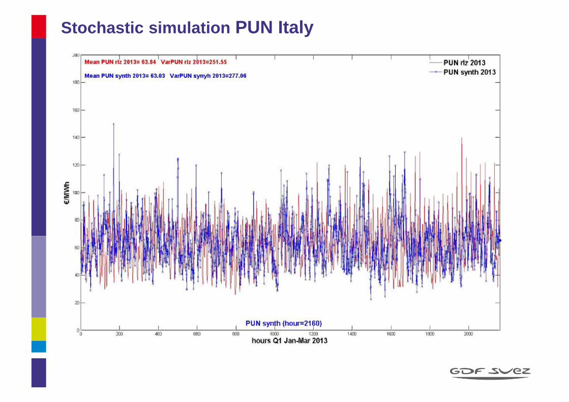
Electricity price PUN modelization

Stochastic simulation PUN Italy
Stochastic simulation PUN Italy
PUN stress Callisto scenario
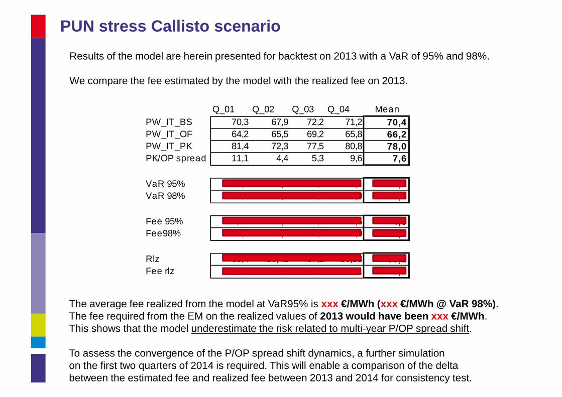
Q_01 Q_02 Q_03 Q_04 MeanPW_IT_BS 70,3 67,9 72,2 71,2 70,4PW_IT_OF 64,2 65,5 69,2 65,8 66,2PW_IT_PK 81,4 72,3 77,5 80,8 78,0PK/OP spread 11,1 4,4 5,3 9,6 7,6
VaR 95% 70,2 70,6 72,5 81,4 73,7VaR 98% 69,8 70,2 72,2 80,9 73,3
Fee 95% 11,25 1,7 4,9 -0,6 4,3Fee98% 11,6 2,1 5,3 0,0 4,7
Rlz 68,4 56,42 67,2 80,88 68,2Fee rlz 13,0 15,9 10,3 -0,1 9,8
Results of the model are herein presented for backtest on 2013 with a VaR of 95% and 98%.
We compare the fee estimated by the model with the realized fee on 2013.
The average fee realized from the model at VaR95% is xxx €/MWh (xxx €/MWh @ VaR 98%).The fee required from the EM on the realized values of 2013 would have been xxx €/MWh.This shows that the model underestimate the risk related to multi-year P/OP spread shift.
To assess the convergence of the P/OP spread shift dynamics, a further simulationon the first two quarters of 2014 is required. This will enable a comparison of the deltabetween the estimated fee and realized fee between 2013 and 2014 for consistency test.

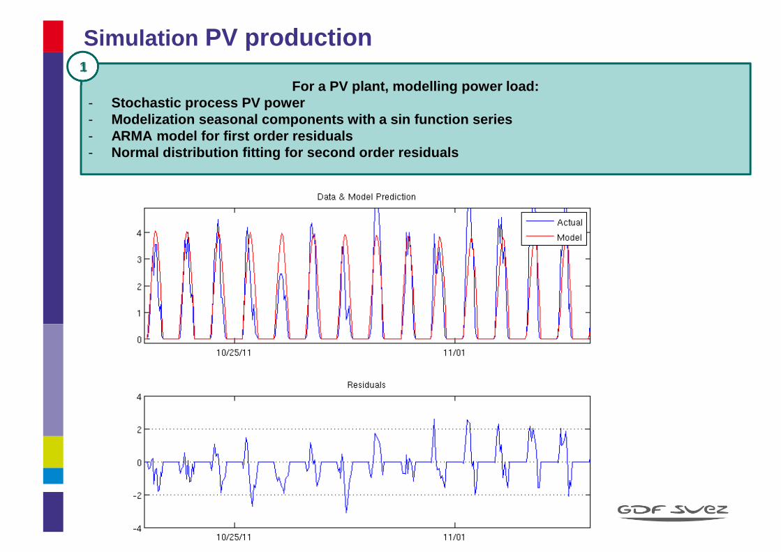
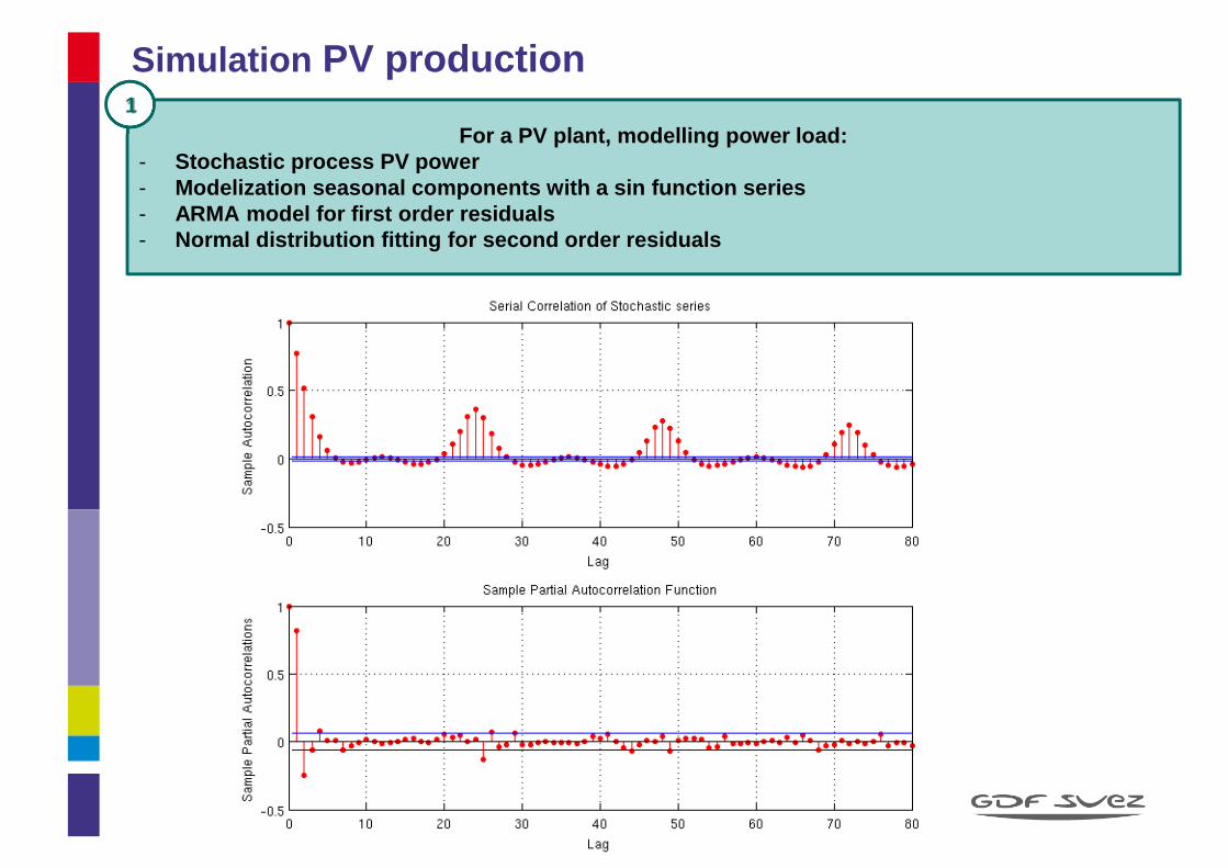
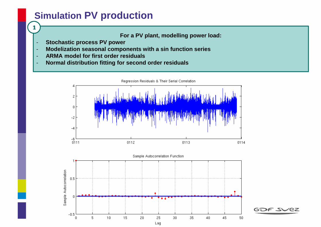
Simulation PV production
For a PV plant, modelling power load:- Stochastic process PV power- Modelization seasonal components with a sin function ser ies- ARMA model for first order residuals- Normal distribution fitting for second order residuals
1
For a PV plant, modelling power load:- Stochastic process PV power- Modelization seasonal components with a sin function ser ies- ARMA model for first order residuals- Normal distribution fitting for second order residuals
1
Simulation PV production
For a PV plant, modelling power load:- Stochastic process PV power- Modelization seasonal components with a sin function ser ies- ARMA model for first order residuals- Normal distribution fitting for second order residuals
1
Simulation PV production
For a PV plant, modelling power load:- Stochastic process PV power- Modelization seasonal components with a sin function ser ies- ARMA model for first order residuals- Normal distribution fitting for second order residuals
1
Simulation PV production

17.2 17.4 17.6 17.8 18 18.2 18.4 18.60
50
100
150
200
250
300
350
400
450
500
MW
N o
bse
rva
tion
s M
on
teca
rlo (
out
of 4
000
pro
cess
es)
Psynth
mean
mean rlz 2010 ≈≈≈≈ 17.9 MW ≈≈≈≈ Q
opt
Pmean ~ Q
Risk Analysis:- Montecarlo simulation assess optimal hedging level (Qopt)
- Montecarlo simulation, with hedging (Qopt) to assess producer Fee e VaR
3
A first MC run generates the wind velocity
and power processes. The frequency
distribution determinates the optimal
hedging level Qopt.
3a
MC simulation for production

Risk Analysis:- Montecarlo simulation assess optimal hedging level (Qopt)
- Montecarlo simulation, with hedging (Qopt) to assess producer Fee e VaR
-3 -2.5 -2 -1.5 -1 -0.5 0 0.5 1 1.5 2 2.5 30
50
100
150
200
250
300
350
400
450
500
€/MWh
N o
bse
rva
tions
Mon
teca
rlo (
out o
f 40
00
pro
cess
es)
Exposure Delta
mean rlz 2010 ≈≈≈≈ -0.28 €/MWh
95%confidence
95%confidence
fee @ 1.5 €/MWh
A second MC run generates the exposure
to PUN of the residual production
above/behind Qopt
The producer fee is at 95% confidence.
VaR 95% ~ Fee
A first MC run generates the wind velocity
and power processes. The frequency
distribution determinates the optimal
hedging level Qopt.
3
MC simulation for residual exposure VaR
3a
3b
