remote sensing of environment - university of … · eddy ﬂux sites are available in na, which...

Remote Sensing of Environment 183 (2016) 154–169

Contents lists available at ScienceDirect

Remote Sensing of Environment

j ourna l homepage: www.e lsev ie r .com/ locate / rse

Consistency between sun-induced chlorophyll fluorescence and grossprimary production of vegetation in North America

Yao Zhang a, Xiangming Xiao a,b,⁎, Cui Jin a, Jinwei Dong a, Sha Zhou c, Pradeep Wagle a, Joanna Joiner d,Luis Guanter e, Yongguang Zhang f, Geli Zhang a, Yuanwei Qin a, Jie Wang a, Berrien Moore III g

a Department of Microbiology and Plant Biology, Center for Spatial Analysis, University of Oklahoma, Norman, OK 73019, USAb Institute of Biodiversity Science, Fudan University, Shanghai 200433, Chinac State Key Laboratory of Hydroscience and Engineering, Department of Hydraulic Engineering, Tsinghua University, Beijing, Chinad NASA Goddard Space Flight Center, Greenbelt, MD, USAe Helmholtz Centre Potsdam, German Research Center for Geosciences (GFZ), Telegrafenberg A17, 14473 Potsdam, Germanyf Jiangsu Provincial Key Laboratory of Geographic Information Science and Technology, International Institute for Earth System Sciences, Nanjing University, 210023 Nanjing, Chinag College of Atmospheric and Geographic Sciences, University of Oklahoma, Norman, OK 73019, USA

⁎ Corresponding author at: Department of MicrobiologSpatial Analysis, University of Oklahoma, Norman, OK 730

E-mail address: [email protected] (X. Xiao).

http://dx.doi.org/10.1016/j.rse.2016.05.0150034-4257/© 2016 Elsevier Inc. All rights reserved.

a b s t r a c t
a r t i c l e i n f o
Article history:Received 16 August 2015Received in revised form 17 May 2016Accepted 23 May 2016Available online xxxx

Accurate estimation of the gross primary production (GPP) of terrestrial ecosystems is vital for a better understand-ing of the spatial-temporal patterns of the global carbon cycle. In this study,we estimateGPP inNorth America (NA)using the satellite-based Vegetation Photosynthesis Model (VPM), MODIS images at 8-day temporal and 500 mspatial resolutions, and NCEP-NARR (National Center for Environmental Prediction-North America RegionalReanalysis) climate data. The simulated GPP (GPPVPM) agrees well with the flux tower derived GPP (GPPEC) at 39AmeriFlux sites (155 site-years). The GPPVPM in 2010 is spatially aggregated to 0.5 by 0.5° grid cells and thencompared with sun-induced chlorophyll fluorescence (SIF) data from Global Ozone Monitoring Instrument 2(GOME-2), which is directly related to vegetation photosynthesis. Spatial distribution and seasonal dynamics ofGPPVPM and GOME-2 SIF show good consistency. At the biome scale, GPPVPM and SIF shows strong linear relation-ships (R2 N 0.95) and small variations in regression slopes (4.60–5.55 g C m−2 day−1/mWm−2 nm−1 sr−1). Thetotal annual GPPVPM in NA in 2010 is approximately 13.53 Pg C year−1, which accounts for ~11.0% of the globalterrestrial GPP and is within the range of annual GPP estimates from six other process-based and data-drivenmodels (11.35–22.23 Pg C year−1). Among the seven models, some models did not capture the spatial pattern ofGOME-2 SIF data at annual scale, especially in Midwest cropland region. The results from this study demonstratethe reliable performance of VPM at the continental scale, and the potential of SIF data being used as a benchmarkto compare with GPP models.

© 2016 Elsevier Inc. All rights reserved.

Keywords:Vegetation Photosynthesis Model (VPM)Light use efficiencyRemote sensingSIFMODISCarbon cycleGPP product

1. Introduction

Carbon dioxide fixed through photosynthesis by terrestrial vegeta-tion is known as gross primary production (GPP) at the ecosystemlevel. Increased carbon uptake during the past decades helped offsetgrowing CO2 emissions from fossil fuel burning and land cover changeand mitigate the increase of atmospheric CO2 concentration and globalclimate warming (Ballantyne, Alden, Miller, Tans, & White, 2012). A va-riety of approaches have been used to estimate GPP of terrestrial ecosys-tems, and they can be grouped into four categories: 1) process-basedGPP models; 2) satellite-based production efficiency models (PEM); 3)data-driven GPP models upscaled from eddy covariance data; and 4)

y and Plant Biology, Center for19, USA.

models based on sun-induced chlorophyll fluorescence (SIF) (Fig. 1).However, large uncertainty still remains regarding the spatial distribu-tion and seasonal dynamics of GPP,which limits our capability to addressscientific questions related to the increasing seasonal amplitude and in-terannual variation of atmospheric CO2 (Forkel et al., 2016; Graven et al.,2013; Poulter et al., 2014). An accurate estimation of GPP at regional andglobal scales is essential for a better understanding of the underlyingmechanisms of ecosystem-climate interactions and ecosystem responseto extreme climate events, such as drought, heat wave, and flood, etc.(Beer et al., 2010; Yu et al., 2013; Zhang et al., 2016).

Many process-based biogeochemical models employ the enzymekinetics theory, most well-known as encapsulated by Farquhar,Caemmerer, and Berry (1980) and its modification for C4 plants(Collatz, Ribas-Carbo, & Berry, 1992). Some process-based modelsemploy the light-use-efficiency (LUE) concept to estimate GPP(Zeng, Mariotti, & Wetzel, 2005). These models also take multiple

http://crossmark.crossref.org/dialog/?doi=10.1016/j.rse.2016.05.015&domain=pdf

http://dx.doi.org/10.1016/j.rse.2016.05.015

mailto:[email protected]

Journal logo

http://dx.doi.org/10.1016/j.rse.2016.05.015

http://www.sciencedirect.com/science/journal/00344257

www.elsevier.com/locate/rse

Fig. 1. A list of different approaches and models (as examples) to estimate gross primary production (GPP) of vegetation.

155Y. Zhang et al. / Remote Sensing of Environment 183 (2016) 154–169

ecological processes into consideration so that they can be coupledwith general circulation models (GCMs) to predict feedbacks relatedto the global warming and CO2 fertilization (Booth et al., 2012;Keenan et al., 2012; Piao et al., 2013; Xia et al., 2014). However,these models are often run at coarse spatial resolution and the simu-lation results vary enormously even with the same set of meteoro-logical input datasets (Coops, Ferster, Waring, & Nightingale, 2009).

The remote sensing based PEMs estimate GPP as the product ofthe energy absorbed by plants (absorbed photosynthetically activeradiation, APAR) and LUE that converts energy to carbon fixed duringthe photosynthesis process (Monteith, 1972). These models can befurther divided into two subcategories (Dong et al., 2015a; Xiao etal., 2004a). The FPARcanopy based models, including the CarnegieAmes Stanford Approach (CASA) (Potter et al., 1993), the MODISGPP algorithm (Photosynthesis, PSN) (Running et al., 2004; Zhao,Heinsch, Nemani, & Running, 2005), and the EC-LUE model (Yuanet al., 2007), use the radiation absorbed by vegetation canopy. TheFPARchl/green based models use radiation absorbed by chlorophyll orgreen leaves and include the Vegetation Photosynthesis Model(VPM) (Xiao et al., 2004a; Xiao et al., 2004b), Greenness and Radia-tion (GR) model (Gitelson et al., 2006), and the Vegetation Index(VI) model (Wu, Niu, & Gao, 2010b).

The eddy covariance (EC) technique provides estimates of GPP bypartitioning measured net ecosystem CO2 exchange (NEE) betweenland and the atmosphere into GPP and ecosystem respiration (Re)(Baldocchi et al., 2001). Over the past decades, the EC techniquehas been widely applied to measure NEE of various biome typesthroughout the world, and a large amount of GPP data (GPPEC) hasbeen accumulated (Baldocchi, 2014; Baldocchi et al., 2001). A num-ber of statistical models have been developed to upscale GPPECfrom individual sites to the regional scales (Jung, Reichstein, &Bondeau, 2009; Jung et al., 2011; Xiao et al., 2010; Xiao et al., 2014;Yang et al., 2007). These algorithms, such as model tree ensembles(MTE) or regression tree approaches, build a series of rules throughdata mining that relate in situ flux observations to satellite-based in-dices and climate data.

Sun-induced chlorophyll fluorescence (SIF), a byproduct of the veg-etation photosynthesis process, has been recently retrieved using mul-tiple satellite platforms/instruments such as the Greenhouse gases

Observing SATellite (GOSAT) (Frankenberg et al., 2011; Guanter et al.,2012; Joiner et al., 2011; Joiner et al., 2012), the Global Ozone Monitor-ing Instrument 2 (GOME-2) (Joiner et al., 2013), and the Orbiting Car-bon Observatory-2 (OCO-2) (Frankenberg et al., 2014). Recent fieldstudies and theory suggest that SIF contains information from bothAPAR and LUE that is complementary to vegetation indices such as thenormalized difference vegetation index (NDVI) (Guanter et al., 2013;Rossini et al., 2015; Yang et al., 2015). A simple regression modelbased on space-borne SIF has been developed to estimate croplandGPP (Guanter et al., 2014). Zhang et al. (2014) have also shown the po-tential of SIF data to improve carbon cycle models and provide accurateprojections of agricultural productivity (Guan et al., 2015).

Over the past several years, a number of studies have run the VPMwith in situ climate data at various eddy flux tower sites. The resultingGPPVPM was evaluated with GPPEC at different ecosystem types, includ-ing forests (Xiao et al., 2004a, 2004b, 2005), croplands (Kalfas, Xiao,Vanegas, Verma, & Suyker, 2011; Wagle, Xiao, & Suyker, 2015), sa-vannas (Jin et al., 2013), and grasslands (He et al., 2014; Wagle et al.,2014). Wu, Munger, Niu, and Kuang (2010a) compared GPP from fourmodels driven by remotely sensed data at the Harvard forest site andfound that VPM performed best in terms of capturing the seasonal dy-namics of GPP. Yuan et al. (2014) compared seven LUE based modelsat 157 eddyflux sites and showed that VPMhad amoderate rank of per-formance. Dong et al. (2015a) used four EVI-based models to estimateGPP of grasslands and croplands under normal and severe drought con-ditions, and reported that VPM performed better than other models incapturing the impacts of drought on GPP. This was mostly becauseVPM uses Land Surface Water Index (LSWI) that is sensitive to waterstress (Wagle et al., 2014, 2015), while the other three models lack awater stress scalar. Recently, simulations of VPM on the regional scale,driven by regional climate data, have been carried out in the Tibetan Pla-teau (He et al., 2014) and China (Chen et al., 2014), where only limitedGPPEC data are available for model calibration and validation.

In this study, we aim to assess the feasibility and performance of theVPM model in estimating GPP across North America (NA) and explorethe relationship between SIF and GPPVPM at continental scale. The selec-tion of theNA as study area is based on two facts: (1) large uncertaintiesexist in the GPP estimates from various models (ranging from 12.2 to32.9 Pg C year−1) (Huntzinger et al., 2012); and (2) a large number of

156 Y. Zhang et al. / Remote Sensing of Environment 183 (2016) 154–169

eddy flux sites are available in NA, which provides an opportunity for athorough validation. The specific objectives of this study are to: (1) im-plement the VPM simulation at the continental scale over NA; (2) eval-uate the performance of VPM at individual sites using GPPEC data from39 flux tower sites (155 site-years); (3) compare GPPVPM with GOME-2 SIF data at 0.5° (latitude/longitude) resolution across NA; and (4)use of GOME-2 SIF as a reference to compare with GPP estimates fromother six models. In this paper, we report (1) multi-year GPPVPM andGPPEC at individual flux tower sites, dependent upon availability ofGPPEC data, and (2) GPPVPM in 2010 across NA.

2. Materials and method

2.1. Regional datasets for VPM simulations across North America

2.1.1. Climate dataThe VPM model uses photosynthetically active radiation (PAR)

and temperature data as climate input data. We use the NationalCenter for Environmental Prediction-North America Regional Re-analysis (NCEP-NARR) datasets (Mesinger et al., 2006) for 2000–2014. The original three hourly data are first aggregated into 8-dayaverages tomatch the temporal resolution of MODIS vegetation indi-ces. The day-time mean air temperature is obtained by averaging thetemperature between 6 am to 6 pm local time. Zhao, Running, andNemani (2006) reported that the NCEP-NARR product overestimatesthe surface shortwave radiation when comparing with the in situ ob-servation at the flux tower sites. Jin et al. (2015) also compared theNCEP-NARR radiation data with in situ radiation measurements at37 AmeriFlux sites and reported a bias correction factor of 0.8. Inthis study, we applied this factor to adjust the radiation data.

In order to run VPM at a 500 m spatial resolution, we use a non-linear spatial interpolation method (Zhao et al., 2005) to downscalethe NCEP-NARR radiation and temperature dataset from the spatialresolution of 0.25° × 0.25° to 500-m. It uses a fourth power of a co-sine function and adopts the weighted distance from the nearestfour grid cells to calculate a value for each output pixel at MODIS res-olution. The distance factor (Di) for the four nearby grid cells can becalculated as follows:

Di ¼ cos4π2� di

dmax

� �� i ¼ 1;2;3;4 ð1Þ

where di and dmax indicate the distance between the center of the500 m MODIS pixel and each of the four vertex grid cells fromNCEP-NARR data, and the maximum distance between the four ver-tex NCEP-NARR grid cells, respectively. For each MODIS pixel, theweight from the four surrounding NCEP-NARR grid cells can becalculated as:

Wi ¼Di

∑4i¼1 Di

ð2Þ

The final value for each interpolated MODIS pixel (V) can beexpressed as a weighted average:

V ¼ ∑4

i¼1Wi�Við Þ ð3Þ

where Vi is the value for the four surrounding grid cell values of NCEP-NARR data.

2.1.2. MODIS data

2.1.2.1. MODIS surface reflectance and vegetation indices. The MODISMOD09A1 surface reflectance product (500 m spatial resolution and8-day temporal resolution) is used to calculate the enhanced vegetationindex (EVI) (Huete et al., 2002) and LSWI as inputs to the VPM. LSWI iscalculated as the normalized difference between NIR (0.78–0.89 μm)and SWIR (1.58–1.75 μm) and is sensitive to water content. Therefore,LSWI is a good indicator of water stress from the vegetation canopyand soil background (Xiao, Boles, Liu, Zhuang, & Liu, 2002). These twoindices are calculated as follows:

EVI ¼ 2:5� ρnir−ρredρnir þ 6� ρred−7:5� ρblueð Þ þ 1

ð4Þ

LSWI ¼ ρnir−ρswir

ρnir þ ρswirð5Þ

A temporal gap-fill algorithm is applied to the EVI time series data.The data quality is checked using the quality flag layer, and those obser-vations not affected by cloud and climatological aerosols are considered‘GOOD’ quality (MOD35 cloud= ‘clear’; aerosol quantity= ‘low’ or ‘av-erage’). Each pixel is temporally linearly interpolated using only good-quality EVI observations within each year. A Savitzky–Golay filter isthen applied to each pixel to eliminate high frequency noise (Chen etal., 2004). If a pixel has fewer than three out of 46 good observationsfor one year, the original data (no gap-filled) are used. Fortunately,this happens only for b0.5% of the total pixels and the majority ofthose are in less productive, boreal areas.

2.1.2.2. MODIS land cover data. The MODIS MCD12Q1 land cover prod-uct at 500-m spatial resolution (Friedl et al., 2010) includes annualland cover types from 2001 to 2013. We use MCD12Q1 data in2001 to represent year 2000, and MDD12Q1 data in 2013 to repre-sent year 2014, which allows us to have a full time series of landcover types for 2000–2014. The IGBP land cover classificationscheme in the dataset is used to provide biome specific informationfor the VPM. A lookup-table (LUT) is used to get the essential param-eters including maximum LUE as well as the maximum, minimum,and optimum temperatures for vegetation photosynthesis (see Ap-pendix Table A1).

In order to investigate the relationship between GPPVPM and SIF(0.5° latitude and longitude resolution) in different vegetation/biome types, we also aggregate the original 500 m land cover datato 0.5° grid cells using the following procedure. The original IGBPland cover data are first merged and reprojected onto the longi-tude-latitude projection with the original spatial resolution.We cal-culate the frequency (number of 500-m pixels) of individualvegetation types within a 0.5° × 0.5° grid cell. Then, for each0.5° × 0.5° grid cell, if one vegetation type is dominant (N75% ofthe grid cell), this grid cell is assigned that vegetation type; if noland cover type is dominant, the grid cell is not assigned a type.

2.1.2.3. MODIS land surface temperature data. TheMODISMYD11A2 landsurface temperature dataset is used to derive the thermal growing sea-son and eliminate the snow cover period, which avoids the effect ofsnow cover in retrieving the yearly maximum LSWI. The MYD11A2dataset is chosen because it provides observations at 1:30 am, whichis close to the daily minimum temperature. For each pixel each year,the thermal growing season is defined using the nighttime land surfacetemperature (Dong et al., 2015b). Once three consecutive 8-day's in thespring have nighttime temperatures above 5°C, the thermal growingseason begins; when three consecutive 8-day's in the fall have night-time temperatures below 10°C, the thermal growing season ends. A de-tailed application of this temperature-based phenology was recentlyreported (Zhang et al., 2015).


2.2. Datasets used to evaluate and compare VPM simulations across NorthAmerica

2.2.1. CO2 eddy flux data from AmeriFlux tower sitesCO2 flux data from 39 AmeriFlux sites are downloaded from the

AmeriFlux data portal (http://ameriflux.ornl.gov/). These flux sitescover most of the major biomes in NA (DBF, ENF, MF, GRA, CRO, CSH,OSH, WET and WSA) (Table 1). The 8-day level-4 gap-filled flux datawith the Marginal Distribution Sampling (MDS) method is used(Reichstein et al., 2005). GPPEC estimates from individual sites areused to evaluate GPPVPM.

2.2.2. Sun-induced chlorophyll fluorescence (SIF) data from GOME-2The latest version (v26) of monthly SIF data from the GOME-2

instrument onboard Eumetsat's MetOp-A satellite is used in thisstudy and available to the public at http://acdb-ext.gsfc.nasa.gov/People/Joiner/my_gifs/GOME_F/GOME-F.htm (Joiner et al., 2014).GOME-2 captures earth radiation in the range from ~600 to800 nm with a spectral resolution of ~0.5 nm at a nominal nadirfootprint of 40 × 80 km2 in the nominal observing configuration.Wavelengths around 740 nm at the far-red peak of the SIF emissionare used for SIF retrievals with a principal component analysis

Table 1Descriptions of the 39 flux tower sites used in this study. IGBP class, R2, and RMSE are the Internnation, and root mean square error of the regression analysis between tower-based gross primodel.

ID NAME LAT LON IGBP class Years

US-Bo1 Bondville 40.0062 −88.2904 CROUS-Ne1 Mead irrigated continuous 41.1651 −96.4766 CROUS-Ne2 Mead irrigated rotation 41.1649 −96.4701 CROUS-Ne3 Mead rainfed rotation 41.1797 −96.4397 CROUS-Ro1 Rosemount- G21 44.7143 −93.0898 CROUS-Ro3 Rosemount- G19 44.7217 −93.0893 CROUS-KS2 Kennedy Space Center 28.6086 −80.6715 CSHUS-Los Lost Creek 46.0827 −89.9792 CSHUS-Bar Bartlett Experimental Forest 44.0646 −71.2881 DBFUS-Ha1 Harvard Forest 42.5378 −72.1715 DBFUS-LPH Little Prospect Hill 42.5419 −72.1850 DBFUS-MMS Morgan Monroe State Forest 39.3232 −86.4131 DBFUS-MOz Missouri Ozark Site 38.7441 −92.2000 DBFUS-UMB Univ. of Mich. Biological Station 45.5598 −84.7138 DBFUS-WCr Willow Creek 45.8059 −90.0799 DBFCA-NS1 UCI-1850 burn site 55.8792 −98.4839 ENFCA-NS2 UCI-1930 burn site 55.9058 −98.5247 ENFCA-NS3 UCI-1964 burn site 55.9117 −98.3822 ENFCA-NS4 UCI-1964 burn site wet 55.9117 −98.3822 ENFCA-NS5 UCI-1981 burn site 55.8631 −98.4850 ENFUS-Blo Blodgett Forest 38.8953 −120.6328 ENFUS-Fmf Flagstaff Managed Forest 35.1426 −111.7273 ENFUS-Ho1 Howland Forest (main tower) 45.2041 −68.7402 ENFUS-Ho2 Howland Forest (west tower) 45.2091 −68.7470 ENFUS-Me2 Metolius-intermediate aged pine 44.4523 −121.5574 ENF 2002,US-Me3 Metolius-second young aged pine 44.3154 −121.6078 ENFUS-Me5 Metolius-first young aged pine 44.4372 −121.5668 ENFUS-NC1 North Carolina Clearcut 35.8115 −76.7115 ENFUS-Wi0 Wisconsin young red pine 46.6188 −91.0814 ENFUS-Wi4 Wisconsin mature red pine 46.7393 −91.1663 ENFUS-ARb ARM SGP burn 35.5497 −98.0402 GRAUS-ARc ARM SGP control 35.5465 −98.0400 GRAUS-Goo Goodwin Creek 34.2547 −89.8735 GRAUS-Wlr Walnut River Watershed 37.5208 −96.8550 GRAUS-Syv Sylvania Wilderness Area 46.2420 −89.3477 MFCA-NS6 UCI-1989 burn site 55.9167 −98.9644 OSHCA-NS7 UCI-1998 burn site 56.6358 −99.9483 OSHUS-Ivo Ivotuk 68.4865 −155.7503 WET 2004,US-FR2 Freeman Ranch-Mesquite Juniper 29.9495 −97.9962 WSA

CRO: cropland; CSH: closed shrublands; DBF: deciduous broadleaf forests; ENF: evergreen neeWSA: woody savannas.

approach to account for atmospheric absorption. The results arethen quality-controlled (e.g., heavily cloud contaminated data re-moved) and aggregated to monthly means at 0.5° × 0.5° spatial res-olution (Joiner et al., 2013). In this study, we use GOME-2 SIF datafor the period from January 2010 to February 2011.

2.2.3. GPP data from other six modelsThe GPP data from the four process-based models (LPJ, LPJ-GUESS,

ORCHIDEE, and VEGAS) are part of the TRENDY projects (Sitch et al.,2008), which intended to compare trends in net land-atmosphere car-bon exchange over the period 1980–2010 (Table 3). These four models,driven by the CRU+ NCEP climate data and global annual atmosphericCO2, are chosen because they have different algorithms to simulate GPPat 0.5° × 0.5° spatial resolution.

Another two models involved in the comparison are the MPI-BGC and MODIS PSN. The MPI-BGC estimates GPP by upscalingglobal CO2 flux observations using aModel Tree Ensemble approach(Jung et al., 2009). MODIS PSN employs a production-efficiency ap-proach and uses the MODIS fraction of photosynthetically active ra-diation product (MOD15A2) and meteorological data (Running etal., 2004). The C55 version of MODIS PSN product (MOD17A2C55) is used.

ational Geosphere-Biosphere Programme land cover classification, coefficient of determi-mary production (GPPEC) and simulated GPP (GPPVPM) using vegetation photosynthesis

used R2 RMSE Reference

2001–2006 0.83 2.20 Hollinger, Bernacchi, and Meyers (2005)2001–2005 0.91 3.06 Suyker, Verma, Burba, and Arkebauer (2005)2001–2005 0.91 2.71 Suyker et al. (2005)2001–2005 0.85 2.76 Suyker et al. (2005)2004–2006 0.80 2.45 Griffis, Baker, and Zhang (2005)2004–2006 0.81 2.22 Griffis et al. (2005)2004–2005 0.72 0.96 Dijkstra et al. (2002)2001–2002 0.90 1.59 Sulman, Desai, Cook, Saliendra, and Mackay (2009)2004–2006 0.93 1.33 Jenkins et al. (2007)2000–2006 0.83 2.05 Urbanski et al. (2007)2001–2005 0.91 1.30 Vanderhoof, Williams, Pasay, and Ghimire (2013)2005–2007 0.91 1.59 Schmid, Grimmond, Cropley, Offerle, and Su (2000)2000–2006 0.89 1.37 Gu et al. (2006)2000–2006 0.97 0.78 Gough, Vogel, Schmid, Su, and Curtis (2008)2002–2005 0.96 1.05 Cook et al. (2004)2003–2005 0.65 1.00 Goulden et al. (2006)2002–2005 0.70 0.88 Goulden et al. (2006)2002–2005 0.92 1.49 Goulden et al. (2006)2003–2004 0.84 1.08 Goulden et al. (2006)2002–2005 0.89 1.13 Goulden et al. (2006)2000–2006 0.74 1.58 Goldstein et al. (2000)2007 0.63 0.95 Dore et al. (2008)2000–2004 0.88 0.84 Hollinger et al. (2004)2000–2004 0.69 0.98 Hollinger et al. (2004)2004–2007 0.91 1.03 Law et al. (2004)2004–2005 0.69 1.26 Law, Williams, Anthoni, Baldocchi, and Unsworth (2000)2000–2002 0.94 0.60 Law et al. (2000)2005–2006 0.95 0.93 Noormets et al. (2010)2002 0.81 1.79 Sun, Noormets, Chen, and McNulty (2008)2002–2005 0.92 0.81 Sun et al. (2008)2005–2006 0.91 1.99 Fischer, Billesbach, Berry, Riley, and Torn (2007)2005–2006 0.91 2.07 Fischer et al. (2007)2004–2006 0.68 1.93 Wilson and Meyers (2007)2002–2004 0.94 0.81 Coulter et al. (2006)2001–2006 0.92 1.12 Desai, Bolstad, Cook, Davis, and Carey (2005)2002–2005 0.87 0.69 Goulden et al. (2006)2002–2005 0.86 0.63 Goulden et al. (2006)2006 0.67 0.80 Epstein, Calef, Walker, Chapin, and Starfield (2004)2004–2006 0.73 1.13 Heinsch et al. (2004)

dleleaf forest; GRA: grassland; MF: mixed forest; OSH: open shrublands; WET: wetland;

http://ameriflux.ornl.gov


2.3. A brief description of the Vegetation Photosynthesis Model (VPM)

The satellite-based VPM (Xiao et al., 2004a, 2004b) uses the productof light use efficiency (LUE, εg), and absorbed photosynthetically activeradiation by chlorophyll (APARchl) to estimate GPP as follows (Fig. 2):

GPP ¼ εg � APARchl ð6Þ

VPMuses the fraction of absorbed photosynthetic active radiation bychlorophyll (fAPARchl) to estimate APARchl. The fAPARchl is estimatedfrom a linear function of EVI where the coefficient α is set to be 1.0(Xiao et al., 2004a).

APARchl ¼ fAPARchl � PAR ð7Þ

fAPARchl ¼ α � EVI ð8Þ

The light-use-efficiency (εg) in the VPM is a down-regulation ofmaximum LUE (ε0) by temperature (Tscalar) and water stress limi-tation (Wscalar) on photosynthesis as follows:

εg ¼ ε0 � Tscalar �Wscalar ð9Þ

ε0 is a biome-specific parameter and differs for C3 and C4 plants. Theε0 values are obtained from a lookup-table (LUT) using the MODIS landcover data. Tscalar is estimated from the equation used in the TerrestrialEcosystem Model (TEM) (Raich et al., 1991).

Tscaler ¼T−T maxð Þ � T−T minð Þ

T−T maxð Þ � T−T minð Þ− T−Topt� �2 ð10Þ

where Tmin, Tmax and Topt are the minimum, maximum, and optimumtemperatures for vegetation photosynthesis, respectively. These

Fig. 2. Flowchart of the data processing procedures

parameters are biome specific and are also obtained from the LUT. Thelimitation from water stress is estimated from LSWI:

Wscalar ¼1þ LSWI

1þ LSWImaxð11Þ

LSWImax is themaximum LSWI during the growing season over sev-eral years. We delineate the LSWImax for plant growing season from thefollowing steps: (1) during the growing season period pre-defined bythe LST, LSWImax is retrieved as the yearly maximum LSWI. If tempera-ture-based identification of the growing season fails in the boreal regionwhere nighttime temperature is always below10°C, the growing seasonis set to be June to August. (2) LSWI will have an abnormally high valueif snow exists and a lower value during drought periods. To eliminatethese abnormal values and take the land cover change into consider-ation,we further calculate the LSWImax using amoving-window statisti-cal algorithm: we select a window of five years and pick the secondlargest maximum LSWI in this period.

3. Results

3.1. Seasonal dynamics of GPP at individual flux tower sites

Fig. 3 shows the seasonal dynamics and interannual variations ofGPPEC and GPPVPM across the 39 flux tower sites. The VPM accuratelypredicts the seasonality and magnitude of GPP for most natural veg-etation (vegetation types other than cropland and cropland/naturalvegetationmosaic in IGBP classification) (Fig. 3). Table 1 summarizesthe correlation between GPPEC and GPPVPM at individual sites overyears. Nearly two thirds of the natural biomes sites have aRMSE b1.5 g C m−2 day−1. Cropland sites have slightly largerRMSE values of 2.20–3.06 g C m−2 day−1.

Fig. 4 shows the comparison between GPPEC and GPPVPM at biomelevels. When compared to GPPEC, GPPVPM underestimate by 4% (accord-ing to regression slope and hereafter) for deciduous broadleaf forests(DBF), 8% for mixed forests (MF), and 16% for evergreen needleleaf for-ests (ENF). GPPVPM and GPPEC agree well for closed shrubland (2%) andopen shrubland (4%). For grassland and woody savannas (WSA), thebiases are b8%. When all natural biome sites are combined, GPPVPM is

for vegetation photosynthesis model (VPM).

Fig. 3. Seasonal dynamics and interannual variations of the tower-based (GPPEC) and the modeled (GPPVPM) gross primary production at 39 flux sites at 8-day intervals. The blue linesrepresent the GPPEC and the black circles represent the GPPVPM. The ticks on the x-axis represent the first date of the corresponding year. (For interpretation of the references to colorin this figure legend, the reader is referred to the web version of this article.)


Fig. 4.A comparison of the tower-based (GPPEC) and themodeled (GPPVPM) gross primaryproduction by biome types. Data are pooled across the study period for each biome. Thedash line is 1:1 line and solid lines are linear regression lines forced to pass the origin.


slightly lower thanGPPEC, approximately 8% (y=0.92x, R2=0.85) (Fig.4). For cropland sites (cropland and cropland/natural vegetationmosaicin IGBP classification), GPPVPM is lower than GPPEC by 23% (y = 0.77x,R2 = 0.82). When all 39 sites are lumped together, the difference be-tween GPPVPM and GPPEC is approximately 13% (y = 0.87x, R2 =0.82). The LUE parameter in VPM improves the predictability of GPP,as represented by the decreased coefficient of determination (R2) in

Fig. 5. Spatial distribution of modeled (A) annual GPPV

the VPM model sensitivity analysis for both natural biomes and all bi-omes sites when LUE parameter is removed (Fig. A1).

3.2. Spatial patterns of GPPVPM across North America in 2010 at 500-mspatial resolution

Fig. 5A shows the spatial distribution of annual GPPVPM for 2010across NA. The highest GPPVPM (N2000 g C m−2 year−1) occurs inthe southernmost tropical regions. GPPVPM decreases along a latitu-dinal gradient in the eastern region, owing to the decreasing temper-ature and growing season length. GPPVPM also decreases along alongitudinal gradient from east (dominated by forest) to west (dom-inated by grasslands and desert). Fig. 5B shows the spatial distribu-tion of the maximum daily GPPVPM in 2010. The highest value is~20 g C m−2 day−1 for the Midwest Corn Belt. The southeasternU.S. has a relatively low value as compared with the mid-latitude re-gion (35°N–45°N). The biggest contrast between annual GPPVPM andmaximum daily GPPVPM is found in the tropical and western coastalregions, where annual GPPVPM is highest while the maximum dailyGPPVPM is moderate.

GPPVPM varies significantly across biomes (Table 2). The most pro-ductive ecosystem is the evergreen broadleaf forest with an annualGPPVPM of N2000 g C m−2 year−1. Open shrubland and savannas arethe least productive with an annual GPPVPM b 375 g C m−2 year−1.Grassland, savannas, and shrublands have relatively high spatial vari-ance because of the extensive distribution and high sensitivity to soilwater. All natural vegetation contribute about 70% of the total GPPVPM,with an average of 600.88 g C m−2 year−1. Croplands accounts forabout 27% of the total GPP but with a nearly doubled photosynthetic ca-pacity (1194.27 g C m−2 year−1) compared with the mean of naturalvegetation. The maximum daily GPPVPM for different biomes variesfrom 3.59 to 12.00 g C m−2 day−1. Croplands have the largest GPPVPMmagnitudes (9.94 to 12.00 g C m−2 day−1). Forest ecosystems have arelatively higher maximum photosynthetic rate (8.79 g C m−2 day−1)compared with other natural vegetation types (4.65 g C m−2 day−1).

PM and (B) maximum daily GPPVPM for year 2010.

Table 2The magnitudes and annual sums of simulated gross primary production (GPPVPM) of different biomes in North America (170°–50°W, 20°–80°N) for year 2010.

IGBP class Average annual GPP(g C m−2 year−1)

Standard deviation of annualGPP (g C m−2 year−1)

Average maximum dailyGPP (g C m−2 day−1)

Standard deviation of maximumdaily GPP (g C m−2 day−1)

Total (Pg C year−1)

ENF 638.45 255.53 5.90 1.55 1.32EBF 2038.76 448.32 9.63 1.71 0.16DBF 1443.95 188.49 11.09 1.47 0.75MF 1030.24 330.46 8.53 1.78 1.94OSH 349.30 224.44 3.59 1.31 1.48WSA 815.81 543.79 6.27 2.29 1.50SAV 377.65 267.02 4.17 1.27 0.20GRA 457.50 380.74 4.24 2.59 2.00WET 539.26 253.98 5.00 1.41 0.21CRO 1157.99 390.54 12.00 3.09 2.15CNV 1248.95 317.55 9.94 1.67 1.54

ENF: evergreen needleleaf forest; EBF: evergreen broadleaf forest; DBF: deciduous broadleaf forest; MF: mixed forest; OSH: open shrubland;WSA: woody savannas; SAV: savannas; GRA:grassland; WET: wetland; CRO: cropland; CNV: cropland/natural vegetation mosaic.


The inconsistency between annual GPPVPM sums and maximum dailyGPPVPM may be mainly attributed to different growing season lengthsthat are affected by temperatures and rainfall.

Fig. 6 shows the frequency distribution of annual GPPVPM andmaximum daily GPPVPM for all pixels in NA and their distribution inthe climate space. N70% of pixels have relatively low productivity,i.e., annual GPPVPM b 1000 g C m−2 year−1 or maximum dailyGPPVPM b 10 g C m−2 day−1. We also plot the distribution of the 39flux tower sites in NA based on the annual and maximum dailyGPPEC (Fig. 6). The distribution of the flux tower sites cover thebroad range of maximum daily GPPVPM, andmost of them are locatedin regions with moderate annual GPP (1000–1800 g C m−2 year−1).

Fig. 6. The frequency distribution of GPPVPM of the (A) annual GPP and (B)maximumdaily GPPmean annual temperature (MAT) mean annual precipitation (MAP) (C, D). The blue curvesmaximum daily GPP for the flux tower sites are from the 39 sites used in our study. BlackPrecipitation data from GPCC (Global Precipitation Climatology Centre) and temperature dreferences to color in this figure legend, the reader is referred to the web version of this article

In the two-dimensional climate space described by mean annualtemperature (MAT) and mean annual precipitation (MAP) (Fig. 6C,D), the flux tower sites distribution covers most of the climatespace. The annual GPPVPM generally increases with MAT mad MAP,while the daily maximum GPPVPM is highest in moderate MAT andMAP regions.

3.3. Spatial-temporal comparison between GPPVPM and SIF across NA in2010 at 0.5 degree spatial resolution

We aggregate the 8-day 500-m GPPVPM estimates to the seasonal(3-month interval) and 0.5° latitude/longitude grid to compare with

compared to theflux site distribution and their distribution in the climate space defined byin (A and B) indicate the frequency distribution calculated from Fig. 5. The annual andcrosses in (C and D) represent the location of 39 flux tower sites in the climate space.ata from NCEP-NARR are used to generate the climate space. (For interpretation of the.)

Fig. 7.A comparison of seasonal average sun-induced fluorescence (SIF) from the GOME-2satellite instrument and simulated gross primary production (GPPVPM) during the periodof March 2010 through February 2011. MAM, JJA, SON, and DJF correspond to spring,summer, fall, and winter, respectively.


the seasonal SIF data. Both GPPVPM and GOME-2 SIF data have strongseasonal dynamics and spatial variation across NA (Figs. 7, 8).

During spring (March to May), both GPPVPM and GOME-2 SIF arerelatively high in the southeastern part of the United States (Fig. 7),where forests dominate and plants grow through the spring. BothGPPVPM and GOME-2 SIF are also high in California, where the Med-iterranean climate (warm and wet spring and dry summer) is locat-ed (Ma, Baldocchi, Xu, & Hehn, 2007; Xu & Baldocchi, 2004). Incomparison, the rest of lands with low temperature and/or rainfallin NA have low GPPVPM and GOME-2 SIF values.

In summer months (June to August), the Corn Belt in mid-west U.S. and southwestern Canada has the highest GPPVPM andSIF. This is supported by the eddy flux data: GPPEC for maize isN25 g C m−2 day−1 during summer, much higher than that ofthe forest ecosystems. Overall, summer months contribute N62% ofthe annual GPP in NA, 42% of which come from Canada and 45%from the conterminous U.S. SIF data also show the highest valuesin the Corn Belt and lowest in the western and northern regions,consistent with the GPPVPM.

In the fall (September to November), both GPPVPM and SIF dropsubstantially in the mid-west region due to crop harvesting. Similarto spring, the high photosynthesis rate also corresponds to a longgrowing season in the southeastern U.S., but the value is smallerthan spring. The eastern and western coasts of Mexico as well asCuba still fix carbon at a rate of N5 g C m−2 day−1. In Alaska andnorthern Canada, all vegetation goes to dormancy, and both GPPVPMand SIF values are close to 0. These spatial patterns are also evident inthe SIF data.

During the winter (December through February), only the verysouthern part of the U.S., California, and coastal regions of Mexico and

Cuba have moderate GPPVPM and SIF values. All the other regions donot show any sign of photosynthesis activities, and both GPPVPM andSIF values are close to zero.

4. Discussion

4.1. The relationship between SIF and GPP

SIF is emitted during the vegetation photosynthetic process.Absorbed energy by chlorophyll is partitioned into SIF, photochem-ical quenching (PQ, energy used for photosynthesis), non-photo-chemical quenching (NPQ, energy partitioned to heating), andefficiency loss (Baker, 2008). Previous studies have shown that SIFis positively correlated with PQ when light is moderate or high orenvironmental stress exists (Flexas, Briantais, Cerovic, & Medrano,2000; Lee et al., 2015; Porcar-Castell, Bäck, Juurola, & Hari, 2006;Soukupová, Cséfalvay, Urban, & Košvancová, 2008). However, therelationship between GPP and SIF emission at far-red peak (SIF740used in our study) is also affected by the SIF contribution from pho-tosystem II and photosystem I, alternative sinks of energy, photo-respiration, internal CO2 concentration of leaves and enzymeactivities, etc. (Porcar-Castell et al., 2014). Although SIF measure-ments from satellite provide a direct and independent estimationsof photosynthetic activity which is different from reflectancebased vegetation indices, the GPP-SIF relationship still needs inten-sive investigation.

Several studies (Joiner et al., 2014; Wagle, Zhang, Jin, & Xiao,2016; Zhang et al., 2014) have reported on the direct comparison be-tween satellite-derived SIF data (0.5° grid cell) and in situGPPEC fromflux sites that often have footprint sizes of a few hundreds of meters,but such comparisons is problematic owing to spatial mismatchesand heterogeneity due to mixed land cover types within a given0.5° grid cell (Zhang et al., 2014). In this study, the VPM simulationsare aggregated to the same spatial resolution as the GOME-2 SIF data.Fig. 8 shows the correlation between GPPVPM and the SIF data for thefour seasons. In spring, summer, and fall, GPPVPM shows a very highcorrelation with SIF. The coefficient of determination ranges from0.74 to 0.86, and the GPPVPM-SIF correlation increases with the in-crease in daily GPP or SIF value (from early to peak growing season).This high spatial correlation confirms our comparison in Section 3.3and can be further explained by the APARchl used in the VPM. BothAPARNDVI (NDVI × PAR) and APARfPAR (fPAR × PAR) have lower cor-relation with SIF compared with APARchl; an obvious saturation canbe found in summer where SIF continues to increase while APARNDVI

and APARfPAR tend to saturate. The regression slope between APARchl

and SIF are also more stable during the growing season (2.82±0.13).As SIF is reemitted from the photosystem II, the higher correlationbetween SIF and APARchl also suggests that EVI can be a good proxyof light absorbed by chlorophyll. In the winter, however, the correla-tions between SIF and GPPVPM and APAR are much weaker mostlydue to the very low SIF signal and relatively lower signal-to-noiseratio. We also calculate the regression between GPPVPM and SIF forpoints with GPPVPM N 1 g Cm−2 day−1 (to eliminate some low valueswith relatively higher bias during the non-growing season). Therange of the regression slopes are narrower when only data for theperiod of GPPVPM N 1 g C m−2 day−1 are used as compared to alldata points (SDslope = 0.42 vs. 0.74).

4.2. Comparison of SIF and GPP estimates in North America from severalmodels

A number of models have reported annual total GPP in NA(Huntzinger et al., 2012; Xiao et al., 2014). The annual GPPVPM is13.53 Pg C in 2010. We further compared GPPVPM with GPP from sixother models (MODIS PSN, MPI-BGC, LPJ, LPJ-GUESS, ORCHIDEE, andVEGAS) (Fig. 9). The VPM-based GPP estimates are close to the average

Fig. 8.Relationship between SIF and GPPVPM (A, E, I, M), APARchl (EVI × PAR) (B, F, J, N), APARNDVI (NDVI × PAR) (C, G, K, O) and APARfPAR (fPAR× PAR) (D, H, L, P) for four seasons (by rowfrom first to fourth: spring, summer, autumn,winter) inNorth America in 2010. EVI andNDVI are frommonthly 0.05°MOD13C1 C5, fPAR is from8-day 1 kmMOD15A2C5, all ofwhich areaggregated to seasonal and 0.5-degree spatial resolution. Black lines are regression for all the points, and the red lines are the regressions between GPPVPM and SIF withGPPVPM N 1 g C m−2 day−1.


of these six models (15.75 Pg C year−1) (Table 3). Three process-basedmodels (LPJ, LPJ-GUESS, and ORCHIDEE) predict very high GPP for thesoutheastern U.S., which may be caused by different approaches theyemployed (enzyme kinetic vs. LUE).

Because SIF is directly retrieved from satellite and has a very goodcorrelation with data driven model-based GPP (Frankenberg et al.,2011; Wagle et al., 2016), we use SIF as a reference to compare thespatial variations in GPP of all models. ORCHIDEE, PSN, MPI-BGC,and VPM show high consistency with SIF data. The major differenceis the relative underestimation at the Corn-Belt and overestimationin the western coast along the U.S./Canada border in ORCHIDEE,PSN, and MPI-BGC. Recent studies reveal that cropland, especiallymaize in the U.S., makes a large contribution to the seasonal swingof atmospheric CO2 concentration (Gray et al., 2014; Zeng et al.,2014). The high GPP values in this region are often underestimatedby models (Guanter et al., 2014). Beer et al. (2010) also suggestthat given the limited C4 vegetation flux data availability, great un-certainty remains in estimating the contribution of C4 plants whileupscaling eddy flux observations. A similar issue is also found in a

study focused on the conterminous U.S. (Xiao et al., 2010), whichmay explain the underestimation of the regional GPP sums. GPPVPMand SIF data show similar spatial patterns for the mid-westernCorn Belt (r = 0.87, p b 0.001) where a previous study showed SIFat a monthly scale has a high correlation with GPP (Guanter et al.,2014); this also supports that the spatial variation of GPPVPM forcroplands is to some degree an improvement over the other sixmodels.

Several previous studies indicate that the relationships betweenGPP and SIF should be different across biomes (Damm et al., 2015;Guanter et al., 2012; Guanter et al., 2014; Parazoo et al., 2014;Verrelst et al., 2015). This ecosystem-dependent GPP-SIF relation-ship is determined by different SIF contribution from both photo-system I and photosystem II, uncertainty in NPQ, and structuralinterference of SIF leaving the canopy (Damm et al., 2015;Verrelst et al., 2015). Here we compare SIF with GPP estimatesfrom three diagnostic models (VPM, MPI-BGC, and MODIS PSN)and APARchl, as well as the relationship between SIFyield (SIF/APARchl) and LUE (Fig. 10). Being consistent with a previous study

Fig. 9. Comparison of annual gross primary production (GPP) from different LUE-basedmodels (A, C), data-driven model (D), process-based models (E, F, G, H), and with sun-induced fluorescence (SIF) (B). Data are shown for the year 2010.


at site level (Yang et al., 2015), we also find that SIF contains the in-formation of LUE, represented by a high correlation between SIFyield(SIF/APARchl) and LUEVPM (Fig. 10E). This also partially supports theGPP-SIF relationship. However, due to the spatial inconsistency, wedid not directly compare GOME-2 SIFyield with LUEEC, more canopyor ecosystem level SIF measurement from in situ or airborne spec-trometers will enable this kind of comparison in the near future.In terms of inter-model comparison, VPM and MPI-BGC showhigher average R2 (0.86 and 0.89, respectively) for individual bi-omes than does MODIS PSN (0.83). The data points are also morescattered in the MODIS PSN than in other two models. Differentbiome types also show distinct differences in slopes (4.03–8.9 forVPM, 3.73–7.83 for MPI-BGC, and 2.76–11.12 for MODIS PSN). Forthemost highly productive biomes (average SIF N 1mWm−2 nm−1-

sr−1), the correlations between predicted GPP and SIF are veryhigh (R2 N 0.95) except for EBF; this may be caused by cloud and/or aerosol contamination of the satellite data. The range of slopesfor these biomes also shows less variation (4.60–5.55 for VPM,

Table 3Annual gross primary production (GPP) of North America (170°–50°W, 20°–80°N) esti-mated from different models for year 2010.

Models Annual GPP (Pg C year−1) Reference

LPJ 22.23 Sitch et al. (2003)LPJ-GUESS 19.84 Smith, Prentice, and Sykes (2001)ORCHIDEE 17.52 Krinner et al. (2005)VEGAS 11.35 Zeng et al. (2005)MODIS GPP 13.13 Zhao et al. (2005)MPI-BGC 12.70 Jung et al. (2011)VPM 13.53 This study

4.02–5.72 for MPI-BGC, and 3.60–6.02 for MODIS PSN). In contrast,the less productive regions usually have lower regression coeffi-cients and more variable slopes. This may be partially due to thehigher relative error for the GOME-2 SIF data (Joiner et al., 2013)and GPP models. SIF retrievals from later satellites (OCO-2, FLEX -Fluorescence Explorer, Sentinel-5 Precursor) will have better accu-racy (Frankenberg et al., 2014; Guanter et al., 2015; Kraft et al.,2013) and can be used to improve and benchmark GPP for landmodels (Lee et al., 2015; Luo et al., 2012; Zhang et al., 2014).

4.3. Sources of uncertainty for VPM simulations in North America

Maps of land cover types affect GPP estimates as the LUE param-eter used in the model varies with biomes. In this study, the MOD12land cover dataset lists croplands as one category and does not dis-tinguish between C3 and C4 crops. Both C3 and C4 crops have differ-ent photosynthetic pathways and light use efficiency (Kalfas et al.,2011; Yuan et al., 2015): C4 crops (e.g., maize) have a higher GPPECthan do C3 crops (Fig. 3). Thus, the LUE parameterization of crop-lands for each year depends upon our knowledge of crop types androtation. For VPM simulations at the continental scale, there arefour options to address this problem in a MODIS cropland pixel: (1)assume 100% C3 plants, (2) assume 100% C4 plants, (3) assumeC3+ C4mixing ratio as 50% each, and (4) use known C3+C4mixingratio from other data sources (in situ data, or other maps). Becausethere is no yearly map of C3/C4 mixing ratio across NA, we simplychose the third option in this study. Therefore, GPPVPM would eitheroverestimate GPP for C3 plants (soybean, wheat, etc.) or underesti-mate for C4 plants (corn, sugar cane, etc.) in those pure pixels. Inthose C3/C4 mixed pixels, however, these artifacts (under- or over-estimation) can be partially alleviated. For example, both maizeand soybean are grown in rotation at the US-Bo1 site within a 50 mradius, but within a 500 m radius of the flux tower site, corn and soy-bean areas have a mixing ratio of 50% each over the years. TheGPPVPM, driven by averaged LUE for C3 and C4 crops, captures boththe seasonality and the magnitude at this site (Fig. 11A). For purepixels, VPM would provide better results if a specific crop type isgiven and an appropriate LUE value is used. We use the LUE valuefor C4 plants at the US-Ne1 site where maize is grown throughoutthe period (Fig. 11B). This modification greatly improves the estima-tion of GPP, with an RMSE reduces from 3.06 to 2.32 g C m−2 day−1

and the slope increases from 0.65 to 0.86.In our study, all croplandflux tower sites are located in themid-west

Corn Belt and altogether we have 16 corn years and 11 soybean years.Aswe use an average LUE of C3 andC4 for croplands, themodelmay un-derestimate GPP at the site scale owing to more corn years (Fig. 4). At aregional scale, the biasmainly depends on the C3 and C4 cropmixing ra-tios within individual pixels. In the U.S. Midwest where C4 crops (e.g.,maize) are dominant, the VPM simulation may underestimate croplandproduction while in California or the Mississippi River Basin, where C3crops are dominant, the VPM simulation may overestimate. Therefore,the lack of crop plant functional type (C3 and C4) is likely the largestsource of uncertainty in the GPPVPM. This clearly highlights the need togenerate annual maps of plant functional types (C3 and C4) in NA inthe near future. In addition, the mismatch between the flux tower foot-print and the MODIS pixel, and the land cover fragmentation withineach MODIS pixel are also critical issues when using EC data for modelvalidation. All flux towers should be evaluated using footprint modelsand high resolution satellite images to provide the representativenessfor the MODIS pixel (Chen et al., 2012).

Image data quality is always an important issue for the applica-tion of remote sensing. In this study, we use the vegetation indicescalculated directly from the MODIS surface reflectance product.These indices are subject to atmospheric contamination (i.e., clouds,aerosols) and often result in a lower-than-normal value for EVI, es-pecially in those regions where cloud and aerosol are persistent

Fig. 10.A comparison for relationship between GPPVPM and SIF (A), GPPMPI and SIF (B), GPPPSN and SIF (C), APARchl (EVI × PAR) and SIF (D), SIFyield (SIF/APAR) and LUEVPM (E) for differentbiome types in North America in 2010. For each month each biome type, a value is given by spatially averaging all the grid cells with in this biome type.


(boreal and tropical regions in our study). The effect of the atmo-spheric contamination can be partially eliminated through a gap-fill method. Fig. 12 shows the comparison between the gap-filledand no gap-filled results. Obvious cloud contamination is marked in

the black ellipse in Fig. 12A, C. The gap-fill method used in ourstudy not only temporally interpolates the low values that aremarked as cloud or aerosol contaminated by the quality controllayer, but also removes the noises caused by other factors. Some

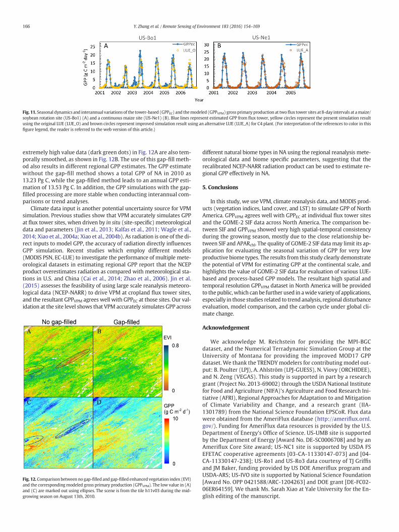
Fig. 11. Seasonal dynamics and interannual variations of the tower-based (GPPEC) and themodeled (GPPVPM) gross primary production at two flux tower sites at 8-day intervals at amaize/soybean rotation site (US-Bo1) (A) and a continuous maize site (US-Ne1) (B). Blue lines represent estimated GPP from flux tower, yellow circles represent the present simulation resultusing the original LUE (LUE_O) and brown circles represent improved simulation result using an alternative LUE (LUE_A) for C4 plant. (For interpretation of the references to color in thisfigure legend, the reader is referred to the web version of this article.)


extremely high value data (dark green dots) in Fig. 12A are also tem-porally smoothed, as shown in Fig. 12B. The use of this gap-fill meth-od also results in different regional GPP estimates. The GPP estimatewithout the gap-fill method shows a total GPP of NA in 2010 as13.23 Pg C, while the gap-filled method leads to an annual GPP esti-mation of 13.53 Pg C. In addition, the GPP simulations with the gap-filled processing are more stable when conducting interannual com-parisons or trend analyses.

Climate data input is another potential uncertainty source for VPMsimulation. Previous studies show that VPM accurately simulates GPPat flux tower sites, when driven by in situ (site-specific) meteorologicaldata and parameters (Jin et al., 2013; Kalfas et al., 2011; Wagle et al.,2014; Xiao et al., 2004a; Xiao et al., 2004b). As radiation is one of the di-rect inputs to model GPP, the accuracy of radiation directly influencesGPP simulation. Recent studies which employ different models(MODIS PSN, EC-LUE) to investigate the performance of multiple mete-orological datasets in estimating regional GPP report that the NCEPproduct overestimates radiation as compared with meteorological sta-tions in U.S. and China (Cai et al., 2014; Zhao et al., 2006). Jin et al.(2015) assesses the feasibility of using large scale reanalysis meteoro-logical data (NCEP-NARR) to drive VPM at cropland flux tower sites,and the resultant GPPVPM agrees well with GPPEC at those sites. Our val-idation at the site level shows that VPM accurately simulates GPP across

Fig. 12. Comparison between no gap-filled and gap-filled enhanced vegetation index (EVI)and the correspondingmodeled gross primary production (GPPVPM). The low value in (A)and (C) are marked out using ellipses. The scene is from the tile h11v03 during the mid-growing season on August 13th, 2010.

different natural biome types in NA using the regional reanalysis mete-orological data and biome specific parameters, suggesting that therecalibrated NCEP-NARR radiation product can be used to estimate re-gional GPP effectively in NA.

5. Conclusions

In this study, we use VPM, climate reanalysis data, andMODIS prod-ucts (vegetation indices, land cover, and LST) to simulate GPP of NorthAmerica. GPPVPM agrees well with GPPEC at individual flux tower sitesand the GOME-2 SIF data across North America. The comparison be-tween SIF and GPPVPM showed very high spatial-temporal consistencyduring the growing season, mostly due to the close relationship be-tween SIF and APARchl. The quality of GOME-2 SIF data may limit its ap-plication for evaluating the seasonal variation of GPP for very lowproductive biome types. The results from this study clearly demonstratethe potential of VPM for estimating GPP at the continental scale, andhighlights the value of GOME-2 SIF data for evaluation of various LUE-based and process-based GPP models. The resultant high spatial andtemporal resolution GPPVPM dataset in North America will be providedto the public,which can be further used in awide variety of applications,especially in those studies related to trend analysis, regional disturbanceevaluation, model comparison, and the carbon cycle under global cli-mate change.

Acknowledgement

We acknowledge M. Reichstein for providing the MPI-BGCdataset, and the Numerical Terradynamic Simulation Group at theUniversity of Montana for providing the improved MOD17 GPPdataset. We thank the TRENDYmodelers for contributing model out-put: B. Poulter (LPJ), A. Ahlström (LPJ-GUESS), N. Viovy (ORCHIDEE),and N. Zeng (VEGAS). This study is supported in part by a researchgrant (Project No. 2013-69002) through the USDA National Institutefor Food and Agriculture (NIFA)'s Agriculture and Food Research Ini-tiative (AFRI), Regional Approaches for Adaptation to and Mitigationof Climate Variability and Change, and a research grant (IIA-1301789) from the National Science Foundation EPSCoR. Flux datawere obtained from the AmeriFlux database (http://ameriflux.ornl.gov/). Funding for AmeriFlux data resources is provided by the U.S.Department of Energy's Office of Science. US-UMB site is supportedby the Department of Energy [Award No. DE-SC0006708] and by anAmeriflux Core Site award; US-NC1 site is supported by USDA FSEFETAC cooperative agreements [03-CA-11330147-073] and [04-CA-11330147-238]; US-Ro1 and US-Ro3 data courtesy of TJ Griffisand JM Baker, funding provided by US DOE Ameriflux program andUSDA-ARS; US-IVO site is supported by National Science Foundation[Award No. OPP 0421588/ARC-1204263] and DOE grant [DE-FC02-06ER64159]. We thank Ms. Sarah Xiao at Yale University for the En-glish editing of the manuscript.




Appendix A

Fig. A1. (A) A comparison betweenGPPEC and APARchl for all 39 sites using 8-day data. (B) comparison between the coefficient of determination (R2) betweenGPPEC vs. GPPVPM, andGPPEC

Table A1Biome specific lookup-table (LUT) used in the VPM model.

IGBP class ENF1 EBF2 DNF DBF1 MF2 CSH2 OSH2 WSA2 SAV2 GRA2 WET CRO3 NVM

Tmin (°C) −1 2 −1 −1 −1 −1 1 −1 1 0 −1 −1 0Topt (°C) 20 28 20 20 19 25 31 24 30 27 20 30 27Tmax (°C) 40 48 40 40 48 48 48 48 48 48 40 48 48ε0 (g C m−2 day−1/W m−2) 0.078 0.078 0.078 0.078 0.078 0.078 0.078 0.078 0.078 0.078 0.078 0.108 0.078

ENF: evergreen needleleaf forest; EBF: evergreen broadleaf forest; DNF: deciduous needleleaf forest; DBF: deciduous broadleaf forests; MF: mixed forest; CSH: closed shrublands; OSH:open shrublands; WSA: woody savannas; SAV: savannas; GRA: grassland; WET: wetland; CRO: cropland; NVM: cropland/natural vegetation mosaic.We use a similar temperature limitation from the Terrestrial Ecosystem Model and the Tmin, Topt, Tmax used in this table are given by 1Aber, Reich, and Goulden (1996), 2McGuire et al.(1992) and 3Wagle et al. (2015) and Kalfas et al. (2011). For some biome types (DNF, WET, NVM) which we did not find reference for temperature parameters, we use parametersfrom similar ecosystems (e.g. ENF for DNF and WET, GRA for NVM). ε0 for C3 plants are estimated from the Wagle et al. (2014), ε0 for C4 crops is from Kalfas et al. (2011). Cropland isregarded as the half-half C3/C4 therefore uses an average value.

vs. APARchl for individual sites.

References

Aber, J. D., Reich, P. B., & Goulden, M. L. (1996). Extrapolating leaf CO2 exchange to thecanopy: A generalized model of forest photosynthesis compared with measurementsby eddy correlation. Oecologia, 106, 257–265.

Baker, N. R. (2008). Chlorophyll fluorescence: A probe of photosynthesis in vivo. Plant Biol:Annu. Rev.

Baldocchi, D. (2014). Measuring fluxes of trace gases and energy between ecosystems andthe atmosphere - The state and future of the eddy covariance method. Global ChangeBiology, 20, 3600–3609.

Baldocchi, D., Falge, E., Gu, L. H., Olson, R., Hollinger, D., Running, S., ... Wofsy, S. (2001).FLUXNET: A new tool to study the temporal and spatial variability of ecosystem-scale carbon dioxide, water vapor, and energy flux densities. Bulletin of theAmerican Meteorological Society, 82, 2415–2434.

Ballantyne, A. P., Alden, C. B., Miller, J. B., Tans, P. P., & White, J. W. (2012). Increase in ob-served net carbon dioxide uptake by land and oceans during the past 50 years.Nature, 488, 70–72.

Beer, C., Reichstein, M., Tomelleri, E., Ciais, P., Jung, M., Carvalhais, N., ... Bonan, G. B.(2010). Terrestrial gross carbon dioxide uptake: Global distribution and covariationwith climate. Science, 329, 834–838.

Booth, B. B. B., Jones, C. D., Collins, M., Totterdell, I. J., Cox, P. M., Sitch, S., ... Lloyd, J. (2012).High sensitivity of future global warming to land carbon cycle processes.Environmental Research Letters, 7, 024002.

Cai, W., Yuan, W., Liang, S., Zhang, X., Dong, W., Xia, J., ... Zhang, Q. (2014). Improved es-timations of gross primary production using satellite-derived photosynthetically ac-tive radiation. Journal of Geophysical Research: Biogeosciences, 119, 110–123.

Chen, B. Z., Coops, N. C., Fu, D., Margolis, H. A., Amiro, B. D., Black, T. A., ... Wofsy, S. C.(2012). Characterizing spatial representativeness of flux tower eddy-covariancemea-surements across the Canadian Carbon Program Network using remote sensing andfootprint analysis. Remote Sensing of Environment, 124, 742–755.

Chen, J., Jönsson, P., Tamura, M., Gu, Z., Matsushita, B., & Eklundh, L. (2004). A simplemethod for reconstructing a high-quality NDVI time-series data set based on theSavitzky–Golay filter. Remote Sensing of Environment, 91, 332–344.

Chen, J., Yan, H., Wang, S., Gao, Y., Huang, M., Wang, J., & Xiao, X. (2014). Estimation ofgross primary productivity in Chinese terrestrial ecosystems by using VPM model.Quaternary Sciences, 34.

Collatz, G. J., Ribas-Carbo, M., & Berry, J. A. (1992). Coupled photosynthesis-stomatal con-ductance model for leaves of C4 plants. Australian Journal of Plant Physiology, 19,519–538.

Cook, B. D., Davis, K. J., Wang, W. G., Desai, A., Berger, B. W., Teclaw, R. M., ... Heilman, W.(2004). Carbon exchange and venting anomalies in an upland deciduous forest innorthern Wisconsin, USA. Agricultural and Forest Meteorology, 126, 271–295.

Coops, N. C., Ferster, C. J., Waring, R. H., & Nightingale, J. (2009). Comparison of threemodelsfor predicting gross primary production across and within forested ecoregions in thecontiguous United States. Remote Sensing of Environment, 113, 680–690.

Coulter, R. L., Pekour, M. S., Cook, D. R., Klazura, G. E., Martin, T. J., & Lucas, J. D. (2006). Sur-face energy and carbon dioxide fluxes above different vegetation types within ABLE.Agricultural and Forest Meteorology, 136, 147–158.

Damm, A., Guanter, L., Verhoef, W., Schläpfer, D., Garbari, S., & Schaepman, M. E. (2015).Impact of varying irradiance on vegetation indices and chlorophyll fluorescence de-rived from spectroscopy data. Remote Sensing of Environment, 156, 202–215.

Desai, A. R., Bolstad, P. V., Cook, B. D., Davis, K. J., & Carey, E. V. (2005). Comparing net eco-system exchange of carbon dioxide between an old-growth and mature forest in theupper Midwest, USA. Agricultural and Forest Meteorology, 128, 33–55.

Dijkstra, P., Hymus, G., Colavito, D., Vieglais, D. A., Cundari, C. M., Johnson, D. P., ... Drake, B.G. (2002). Elevated atmospheric CO2 stimulates aboveground biomass in a fire-re-generated scrub-oak ecosystem. Global Change Biology, 8, 90–103.

Dong, J. W., Xiao, X. M., Kou, W. L., Qin, Y. W., Zhang, G. L., Li, L., ... Moore, B. (2015b).Tracking the dynamics of paddy rice planting area in 1986–2010 through time seriesLandsat images and phenology-based algorithms. Remote Sensing of Environment,160, 99–113.

http://refhub.elsevier.com/S0034-4257(16)30216-4/rf0005




















































Dong, J., Xiao, X., Wagle, P., Zhang, G., Zhou, Y., Jin, C., ... Moore Iii, B. (2015a). Comparisonof four EVI-based models for estimating gross primary production of maize and soy-bean croplands and tallgrass prairie under severe drought. Remote Sensing ofEnvironment, 162, 154–168.

Dore, S., Kolb, T. E., Montes-Helu, M., Sullivan, B. W., Winslow, W. D., Hart, S. C., ...Hungate, B. A. (2008). Long-term impact of a stand-replacing fire on ecosystemCO(2) exchange of a ponderosa pine forest. Global Change Biology, 14, 1801–1820.

Epstein, H. E., Calef, M. P., Walker, M. D., Chapin, F. S., & Starfield, A. M. (2004). Detectingchanges in arctic tundra plant communities in response to warming over decadaltime scales. Global Change Biology, 10, 1325–1334.

Farquhar, G. D., Caemmerer, S. V., & Berry, J. A. (1980). A biochemical-model of photosyn-thetic Co2 assimilation in leaves of C-3 species. Planta, 149, 78–90.

Fischer, M. L., Billesbach, D. P., Berry, J. A., Riley,W. J., & Torn, M. S. (2007). Spatiotemporalvariations in growing season exchanges of CO2, H2O, and sensible heat in agriculturalfields of the southern Great Plains. Earth Interactions, 11.

Flexas, J., Briantais, J. M., Cerovic, Z., & Medrano, H. (2000). Steady-state and maximumchlorophyll fluorescence responses to water stress in grapevine leaves: A new remotesensing system. Remote Sensing of Environment, 73, 283–297.

Forkel, M., Carvalhais, N., Rodenbeck, C., Keeling, R., Heimann, M., Thonicke, K., ...Reichstein, M. (2016). Enhanced seasonal CO2 exchange caused by amplified plantproductivity in northern ecosystems. Science, 351, 696–699.

Frankenberg, C., Fisher, J. B., Worden, J., Badgley, G., Saatchi, S. S., Lee, J. E., ... Yokota, T.(2011). New global observations of the terrestrial carbon cycle from GOSAT: Patternsof plant fluorescence with gross primary productivity. Geophysical Research Letters,38.

Frankenberg, C., O'Dell, C., Berry, J., Guanter, L., Joiner, J., Köhler, P., ... Taylor, T. E. (2014).Prospects for chlorophyll fluorescence remote sensing from the Orbiting Carbon Ob-servatory-2. Remote Sensing of Environment, 147, 1–12.

Friedl, M. A., Sulla-Menashe, D., Tan, B., Schneider, A., Ramankutty, N., Sibley, A., &Huang, X. M. (2010). MODIS Collection 5 global land cover: Algorithm refine-ments and characterization of new datasets. Remote Sensing of Environment,114, 168–182.

Gitelson, A. A., Vina, A., Verma, S. B., Rundquist, D. C., Arkebauer, T. J., Keydan, G., ... Suyker,A. E. (2006). Relationship between gross primary production and chlorophyll contentin crops: Implications for the synoptic monitoring of vegetation productivity. Journalof Geophysical Research-Atmospheres, 111.

Goldstein, A. H., Hultman, N. E., Fracheboud, J. M., Bauer, M. R., Panek, J. A., Xu, M., ...Baugh,W. (2000). Effects of climate variability on the carbon dioxide, water, and sen-sible heat fluxes above a ponderosa pine plantation in the Sierra Nevada (CA).Agricultural and Forest Meteorology, 101, 113–129.

Gough, C. M., Vogel, C. S., Schmid, H. P., Su, H. B., & Curtis, P. S. (2008). Multi-year conver-gence of biometric and meteorological estimates of forest carbon storage. Agriculturaland Forest Meteorology, 148, 158–170.

Goulden, M. L., Winston, G. C., McMillan, A. M. S., Litvak, M. E., Read, E. L., Rocha, A. V., &Elliot, J. R. (2006). An eddy covariance mesonet to measure the effect of forest age onland-atmosphere exchange. Global Change Biology, 12, 2146–2162.

Graven, H. D., Keeling, R. F., Piper, S. C., Patra, P. K., Stephens, B. B., Wofsy, S. C., ... Bent, J. D.(2013). Enhanced seasonal exchange of CO2 by northern ecosystems since 1960.Science, 341, 1085–1089.

Gray, J. M., Frolking, S., Kort, E. A., Ray, D. K., Kucharik, C. J., Ramankutty, N., & Friedl, M. A.(2014). Direct human influence on atmospheric CO2 seasonality from increasedcropland productivity. Nature, 515, 398–401.

Griffis, T. J., Baker, J. M., & Zhang, J. (2005). Seasonal dynamics and partitioning of isotopicCO2 exchange in C-3/C-4 managed ecosystem. Agricultural and Forest Meteorology,132, 1–19.

Gu, L. H., Meyers, T., Pallardy, S. G., Hanson, P. J., Yang, B., Heuer, M., ... Wullschleger, S. D.(2006). Direct and indirect effects of atmospheric conditions and soil moisture onsurface energy partitioning revealed by a prolonged drought at a temperate forestsite. Journal of Geophysical Research-Atmospheres, 111.

Guan, K., Berry, J. A., Zhang, Y., Joiner, J., Guanter, L., Badgley, G., & Lobell, D. B. (2015). Im-proving the monitoring of crop productivity using spaceborne solar-induced fluores-cence. Global Change Biology. http://dx.doi.org/10.1111/gcb.13136.

Guanter, L., Aben, I., Tol, P., Krijger, J. M., Hollstein, A., Kohler, P., ... Landgraf, J. (2015). Po-tential of the TROPOspheric Monitoring Instrument (TROPOMI) onboard the Senti-nel-5 Precursor for the monitoring of terrestrial chlorophyll fluorescence.Atmospheric Measurement Techniques, 8, 1337–1352.

Guanter, L., Frankenberg, C., Dudhia, A., Lewis, P. E., Gomez-Dans, J., Kuze, A., ... Grainger,R. G. (2012). Retrieval and global assessment of terrestrial chlorophyll fluorescencefrom GOSAT space measurements. Remote Sensing of Environment, 121, 236–251.

Guanter, L., Rossini, M., Colombo, R., Meroni, M., Frankenberg, C., Lee, J. E., & Joiner, J.(2013). Using field spectroscopy to assess the potential of statistical approaches forthe retrieval of sun-induced chlorophyll fluorescence from ground and space.Remote Sensing of Environment, 133, 52–61.

Guanter, L., Zhang, Y., Jung, M., Joiner, J., Voigt, M., Berry, J. A., ... Griffis, T. J. (2014). Globaland time-resolved monitoring of crop photosynthesis with chlorophyll fluorescence.Proceedings of the National Academy of Sciences of the United States of America, 111,E1327–E1333.

He, H. L., Liu, M., Xiao, X. M., Ren, X. L., Zhang, L., Sun, X. M., ... Yu, G. R. (2014). Large-scaleestimation and uncertainty analysis of gross primary production in Tibetan alpinegrasslands. Journal of Geophysical Research-Biogeosciences, 119, 466–486.

Heinsch, F. A., Heilman, J. L., McInnes, K. J., Cobos, D. R., Zuberer, D. A., & Roelke, D. L.(2004). Carbon dioxide exchange in a high marsh on the Texas Gulf Coast: Effectsof freshwater availability. Agricultural and Forest Meteorology, 125, 159–172.

Hollinger, D. Y., Aber, J., Dail, B., Davidson, E. A., Goltz, S. M., Hughes, H., ... Walsh, J. (2004).Spatial and temporal variability in forest-atmosphere CO2 exchange. Global ChangeBiology, 10, 1689–1706.

Hollinger, S. E., Bernacchi, C. J., & Meyers, T. P. (2005). Carbon budget of mature no-tillecosystem in North Central Region of the United States. Agricultural and ForestMeteorology, 130, 59–69.

Huete, A., Didan, K., Miura, T., Rodriguez, E. P., Gao, X., & Ferreira, L. G. (2002). Overview ofthe radiometric and biophysical performance of the MODIS vegetation indices.Remote Sensing of Environment, 83, 195–213.

Huntzinger, D. N., Post, W. M., Wei, Y., Michalak, A. M., West, T. O., Jacobson, A. R., ... Cook,R. (2012). North American Carbon Program (NACP) regional interim synthesis: Ter-restrial biospheric model intercomparison. Ecological Modelling, 232, 144–157.

Jenkins, J. P., Richardson, A. D., Braswell, B. H., Ollinger, S. V., Hollinger, D. Y., & Smith, M. L.(2007). Refining light-use efficiency calculations for a deciduous forest canopy usingsimultaneous tower-based carbon flux and radiometric measurements. Agriculturaland Forest Meteorology, 143, 64–79.

Jin, C., Xiao, X. M., Merbold, L., Arneth, A., Veenendaal, E., & Kutsch, W. L. (2013). Phenol-ogy and gross primary production of two dominant savannawoodland ecosystems inSouthern Africa. Remote Sensing of Environment, 135, 189–201.

Jin, C., Xiao, X., Wagle, P., Griffis, T., Dong, J., Wu, C., & Qin, Y. (2015). Effects of in-situand reanalysis climate data on estimation of cropland gross primary productionusing the Vegetation Photosynthesis Model. Agricultural and Forest Meteorology,213, 240.

Joiner, J., Guanter, L., Lindstrot, R., Voigt, M., Vasilkov, A. P., Middleton, E. M., ...Frankenberg, C. (2013). Global monitoring of terrestrial chlorophyll fluorescencefrom moderate-spectral-resolution near-infrared satellite measurements: Methodol-ogy, simulations, and application to GOME-2. Atmospheric Measurement Techniques, 6,2803–2823.

Joiner, J., Yoshida, Y., Vasilkov, A. P., Middleton, E. M., Campbell, P. K. E., Yoshida, Y., ...Corp, L. A. (2012). Filling-in of near-infrared solar lines by terrestrial fluorescenceand other geophysical effects: Simulations and space-based observations fromSCIAMACHY and GOSAT. Atmospheric Measurement Techniques, 5, 809–829.

Joiner, J., Yoshida, Y., Vasilkov, A. P., Schaefer, K., Jung, M., Guanter, L., ... Belelli Marchesini,L. (2014). The seasonal cycle of satellite chlorophyll fluorescence observations and itsrelationship to vegetation phenology and ecosystem atmosphere carbon exchange.Remote Sensing of Environment, 152, 375–391.

Joiner, J., Yoshida, Y., Vasilkov, A. P., Yoshida, Y., Corp, L. A., & Middleton, E. M. (2011). Firstobservations of global and seasonal terrestrial chlorophyll fluorescence from space.Biogeosciences, 8, 637–651.

Jung, M., Reichstein, M., & Bondeau, A. (2009). Towards global empirical upscaling ofFLUXNET eddy covariance observations: Validation of a model tree ensemble ap-proach using a biosphere model. Biogeosciences, 6, 2001–2013.

Jung, M., Reichstein, M., Margolis, H. A., Cescatti, A., Richardson, A. D., Arain, M. A., ...Williams, C. (2011). Global patterns of land-atmosphere fluxes of carbon dioxide, la-tent heat, and sensible heat derived from eddy covariance, satellite, and meteorolog-ical observations. Journal of Geophysical Research-Biogeosciences, 116.

Kalfas, J. L., Xiao, X., Vanegas, D. X., Verma, S. B., & Suyker, A. E. (2011). Modeling gross pri-mary production of irrigated and rain-fed maize using MODIS imagery and CO2 fluxtower data. Agricultural and Forest Meteorology, 151, 1514–1528.

Keenan, T. F., Baker, I., Barr, A., Ciais, P., Davis, K., Dietze, M., ... Richardson, A. D. (2012).Terrestrial biosphere model performance for inter-annual variability of land-atmo-sphere CO2 exchange. Global Change Biology, 18, 1971–1987.

Kraft, S., Bézy, J. L., Del Bello, U., Berlich, R., Drusch, M., Franco, R., ... Silvestrin, P. (2013).FLORIS: Phase A status of the fluorescence imaging spectrometer of the Earth Explor-er mission candidate FLEX. Proc. SPIE 8889, Sensors, Systems, and Next-Generation Sat-ellites XVII. 8889. (pp. 88890T–888812).

Krinner, G., Viovy, N., de Noblet-Ducoudre, N., Ogee, J., Polcher, J., Friedlingstein, P., ...Prentice, I. C. (2005). A dynamic global vegetation model for studies of the coupledatmosphere-biosphere system. Global Biogeochemical Cycles, 19.

Law, B. E., Turner, D., Campbell, J., Sun, O. J., Van Tuyl, S., Ritts, W. D., & Cohen, W. B.(2004). Disturbance and climate effects on carbon stocks and fluxes across WesternOregon USA. Global Change Biology, 10, 1429–1444.

Law, B. E., Williams, M., Anthoni, P. M., Baldocchi, D. D., & Unsworth, M. H. (2000). Measur-ing and modelling seasonal variation of carbon dioxide and water vapour exchange ofa Pinus ponderosa forest subject to soil water deficit. Global Change Biology, 6, 613–630.

Lee, J. E., Berry, J. A., van der Tol, C., Yang, X., Guanter, L., Damm, A., ... Frankenberg, C.(2015). Simulations of chlorophyll fluorescence incorporated into the CommunityLand Model version 4. Global Change Biology, 21, 3469–3477. http://dx.doi.org/10.1111/gcb.12948.

Luo, Y. Q., Randerson, J. T., Abramowitz, G., Bacour, C., Blyth, E., Carvalhais, N., ... Zhou, X. H.(2012). A framework for benchmarking land models. Biogeosciences, 9, 3857–3874.

Ma, S. Y., Baldocchi, D. D., Xu, L. K., & Hehn, T. (2007). Inter-annual variability in carbondioxide exchange of an oak/grass savanna and open grassland in California.Agricultural and Forest Meteorology, 147, 157–171.

McGuire, A. D., Melillo, J., Joyce, L., Kicklighter, D., Grace, A., Moore, B., & Vorosmarty, C.(1992). Interactions between carbon and nitrogen dynamics in estimating net prima-ry productivity for potential vegetation in North America. Global BiogeochemicalCycles, 6, 101–124.

Mesinger, F., DiMego, G., Kalnay, E., Mitchell, K., Shafran, P. C., Ebisuzaki, W., ... Shi, W.(2006). North American regional reanalysis. Bulletin of the American MeteorologicalSociety, 87, 343.

Monteith, J. L. (1972). Solar-radiation and productivity in tropical ecosystems. Journal ofApplied Ecology, 9, 747–766.

Noormets, A., Gavazzi, M. J., Mcnulty, S. G., Domec, J. C., Sun, G., King, J. S., & Chen, J. Q.(2010). Response of carbon fluxes to drought in a coastal plain loblolly pine forest.Global Change Biology, 16, 272–287.

Parazoo, N. C., Bowman, K., Fisher, J. B., Frankenberg, C., Jones, D. B., Cescatti, A., ...Montagnani, L. (2014). Terrestrial gross primary production inferred from satellitefluorescence and vegetation models. Global Change Biology, 20, 3103–3121.

















































http://dx.doi.org/10.1111/gcb.13136



























































































Piao, S., Sitch, S., Ciais, P., Friedlingstein, P., Peylin, P., Wang, X., ... Zeng, N. (2013). Evalu-ation of terrestrial carbon cycle models for their response to climate variability and toCO2 trends. Global Change Biology, 19, 2117–2132.

Porcar-Castell, A., Bäck, J., Juurola, E., & Hari, P. (2006). Dynamics of the energy flowthrough photosystem II under changing light conditions: A model approach.Functional Plant Biology, 33, 229–239. http://dx.doi.org/10.1071/FP05133.

Porcar-Castell, A., Tyystjarvi, E., Atherton, J., van der Tol, C., Flexas, J., Pfundel, E. E., ... Berry,J. A. (2014). Linking chlorophyll a fluorescence to photosynthesis for remote sensingapplications: Mechanisms and challenges. Journal of Experimental Botany, 65,4065–4095.

Potter, C. S., Randerson, J. T., Field, C. B., Matson, P. A., Vitousek, P. M., Mooney, H. A., &Klooster, S. A. (1993). Terrestrial ecosystem production - A process model-based onglobal satellite and surface data. Global Biogeochemical Cycles, 7, 811–841.

Poulter, B., Frank, D., Ciais, P., Myneni, R. B., Andela, N., Bi, J., ... van der Werf, G. R. (2014).Contribution of semi-arid ecosystems to interannual variability of the global carboncycle. Nature, 509, 600–603.

Raich, J., Rastetter, E., Melillo, J., Kicklighter, D., Steudler, P., Peterson, B., ... Vorosmarty, C.(1991). Potential net primary productivity in South America: Application of a globalmodel. Ecological Applications, 1, 399–429.

Reichstein, M., Falge, E., Baldocchi, D., Papale, D., Aubinet, M., Berbigier, P., ...Valentini, R. (2005). On the separation of net ecosystem exchange into assimila-tion and ecosystem respiration: Review and improved algorithm. Global ChangeBiology, 11, 1424–1439.

Rossini, M., Nedbal, L., Guanter, L., Ač, A., Alonso, L., Burkart, A., ... Rascher, U. (2015). Redand far-red sun-induced chlorophyll fluorescence as a measure of plant photosynthe-sis. Geophysical Research Letters n/a-n/a.

Running, S. W., Nemani, R. R., Heinsch, F. A., Zhao, M. S., Reeves, M., & Hashimoto, H.(2004). A continuous satellite-derived measure of global terrestrial primary produc-tion. Bioscience, 54, 547–560.

Schmid, H. P., Grimmond, C. S. B., Cropley, F., Offerle, B., & Su, H. B. (2000). Measurementsof CO2 and energy fluxes over a mixed hardwood forest in the mid-western UnitedStates. Agricultural and Forest Meteorology, 103, 357–374.

Sitch, S., Huntingford, C., Gedney, N., Levy, P. E., Lomas, M., Piao, S. L., ... Woodward, F. I.(2008). Evaluation of the terrestrial carbon cycle, future plant geography and cli-mate–carbon cycle feedbacks using five Dynamic Global Vegetation Models(DGVMs). Global Change Biology, 14, 2015–2039.

Sitch, S., Smith, B., Prentice, I. C., Arneth, A., Bondeau, A., Cramer, W., ... Venevsky, S.(2003). Evaluation of ecosystem dynamics, plant geography and terrestrial car-bon cycling in the LPJ dynamic global vegetation model. Global Change Biology,9, 161–185.

Smith, B., Prentice, I. C., & Sykes, M. T. (2001). Representation of vegetation dynamics inthe modelling of terrestrial ecosystems: Comparing two contrasting approacheswithin European climate space. Global Ecology and Biogeography, 10, 621–637.

Soukupová, J., Cséfalvay, L., Urban, O., Košvancová, M., Marek, M., Rascher, U., ... Nedbal, L.(2008). Annual variation of the steady-state chlorophyll fluorescence emission of ev-ergreen plants in temperate zone. Functional Plant Biology, 35, 63–76. http://dx.doi.org/10.1071/FP07158.

Sulman, B. N., Desai, A. R., Cook, B. D., Saliendra, N., & Mackay, D. S. (2009). Contrastingcarbon dioxide fluxes between a drying shrub wetland in Northern Wisconsin,USA, and nearby forests. Biogeosciences, 6, 1115–1126.

Sun, G., Noormets, A., Chen, J., & McNulty, S. G. (2008). Evapotranspiration estimates fromeddy covariance towers and hydrologic modeling in managed forests in NorthernWisconsin, USA. Agricultural and Forest Meteorology, 148, 257–267.

Suyker, A. E., Verma, S. B., Burba, G. G., & Arkebauer, T. J. (2005). Gross primary productionand ecosystem respiration of irrigated maize and irrigated soybean during a growingseason. Agricultural and Forest Meteorology, 131, 180–190.

Urbanski, S., Barford, C., Wofsy, S., Kucharik, C., Pyle, E., Budney, J., ... Munger, J. W. (2007).Factors controlling CO2 exchange on timescales from hourly to decadal at HarvardForest. Journal of Geophysical Research-Biogeosciences, 112.

Vanderhoof, M., Williams, C., Pasay, M., & Ghimire, B. (2013). Controls on the rate of CO2emission from woody debris in clearcut and coniferous forest environments.Biogeochemistry, 114, 299–311.

Verrelst, J., Rivera, J. P., van der Tol, C., Magnani, F., Mohammed, G., & Moreno, J. (2015).Global sensitivity analysis of the SCOPE model: What drives simulated canopy-leav-ing sun-induced fluorescence? Remote Sensing of Environment, 166, 8–21.

Wagle, P., Xiao, X. M., & Suyker, A. E. (2015). Estimation and analysis of gross primary pro-duction of soybean under various management practices and drought conditions.ISPRS Journal of Photogrammetry and Remote Sensing, 99, 70–83.

Wagle, P., Xiao, X., Torn, M. S., Cook, D. R., Matamala, R., Fischer, M. L., ... Biradar, C. (2014).Sensitivity of vegetation indices and gross primary production of tallgrass prairie tosevere drought. Remote Sensing of Environment, 152, 1–14.

Wagle, P., Zhang, Y., Jin, C., & Xiao, X. (2016). Comparison of solar-induced chlorophyllfluorescence, light-use efficiency, and process-based GPP models in maize.Ecological Applications.. http://dx.doi.org/10.1890/15-1434.1.

Wilson, T. B., & Meyers, T. P. (2007). Determining vegetation indices from solar and pho-tosynthetically active radiation fluxes. Agricultural and Forest Meteorology, 144,160–179.

Wu, C. Y., Munger, J. W., Niu, Z., & Kuang, D. (2010a). Comparison of multiple models forestimating gross primary production using MODIS and eddy covariance data in Har-vard Forest. Remote Sensing of Environment, 114, 2925–2939.

Wu, C. Y., Niu, Z., & Gao, S. A. (2010b). Gross primary production estimation from MODISdata with vegetation index and photosynthetically active radiation in maize. Journalof Geophysical Research-Atmospheres, 115.

Xia, J., Chen, J., Piao, S., Ciais, P., Luo, Y., & Wan, S. (2014). Terrestrial carbon cycle affectedby non-uniform climate warming. Nature Geoscience, 7, 173–180.

Xiao, X., Boles, S., Liu, J., Zhuang, D., & Liu, M. (2002). Characterization of forest types inNortheastern China, using multi-temporal SPOT-4 VEGETATION sensor data. RemoteSensing of Environment, 82, 335–348.

Xiao, X., Hollinger, D., Aber, J., Goltz, M., Davidson, E. A., Zhang, Q., & Moore, B. (2004a).Satellite-based modeling of gross primary production in an evergreen needleleaf for-est. Remote Sensing of Environment, 89, 519–534.

Xiao, J. F., Ollinger, S. V., Frolking, S., Hurtt, G. C., Hollinger, D. Y., Davis, K. J., ... Suyker, A. E.(2014). Data-driven diagnostics of terrestrial carbon dynamics over North America.Agricultural and Forest Meteorology, 197, 142–157.

Xiao, X., Zhang, Q., Braswell, B., Urbanski, S., Boles, S., Wofsy, S., ... Ojima, D. (2004b).Modeling gross primary production of temperate deciduous broadleaf forest usingsatellite images and climate data. Remote Sensing of Environment, 91, 256–270.

Xiao, X. M., Zhang, Q. Y., Saleska, S., Hutyra, L., De Camargo, P., Wofsy, S., ... Moore, B.(2005). Satellite-based modeling of gross primary production in a seasonally moisttropical evergreen forest. Remote Sensing of Environment, 94, 105–122.

Xiao, J., Zhuang, Q., Law, B. E., Chen, J., Baldocchi, D. D., Cook, D. R., ... Ma, S. (2010). A con-tinuous measure of gross primary production for the conterminous United States de-rived fromMODIS and AmeriFlux data. Remote Sensing of Environment, 114, 576–591.

Xu, L. K., & Baldocchi, D. D. (2004). Seasonal variation in carbon dioxide exchange over aMediterranean annual grassland in California. Agricultural and Forest Meteorology,123, 79–96.

Yang, F. H., Ichii, K., White, M. A., Hashimoto, H., Michaelis, A. R., Votava, P., ... Nemani, R. R.(2007). Developing a continental-scalemeasure of gross primary production by com-bining MODIS and AmeriFlux data through Support Vector Machine approach.Remote Sensing of Environment, 110, 109–122.

Yang, X., Tang, J., Mustard, J. F., Lee, J. -E., Rossini, M., Joiner, J., ... Richardson, A. D. (2015).Solar-induced chlorophyll fluorescence correlates with canopy photosynthesis on di-urnal and seasonal scales in a temperate deciduous forest. Geophysical ResearchLetters n/a-n/a.

Yu, G. R., Zhu, X. J., Fu, Y. L., He, H. L., Wang, Q. F., Wen, X. F., ... Tong, C. L. (2013). Spatialpatterns and climate drivers of carbon fluxes in terrestrial ecosystems of China. GlobalChange Biology, 19, 798–810.

Yuan, W., Cai, W., Nguy-Robertson, A. L., Fang, H., Suyker, A. E., Chen, Y., ... Zhang, H.(2015). Uncertainty in simulating gross primary production of cropland ecosystemfrom satellite-based models. Agricultural and Forest Meteorology, 207, 48–57.

Yuan, W., Cai, W., Xia, J., Chen, J., Liu, S., Dong, W., ... Wohlfahrt, G. (2014). Global compar-ison of light use efficiency models for simulating terrestrial vegetation gross primaryproduction based on the LaThuile database. Agricultural and Forest Meteorology, 192-193, 108–120.

Yuan, W., Liu, S., Zhou, G., Zhou, G., Tieszen, L. L., Baldocchi, D., ... Wofsy, S. C. (2007). De-riving a light use efficiency model from eddy covariance flux data for predicting dailygross primary production across biomes. Agricultural and Forest Meteorology, 143,189–207.

Zeng, N., Mariotti, A., & Wetzel, P. (2005). Terrestrial mechanisms of interannual CO(2)variability. Global Biogeochemical Cycles, 19.

Zeng, N., Zhao, F., Collatz, G. J., Kalnay, E., Salawitch, R. J., West, T. O., & Guanter, L. (2014).Agricultural Green Revolution as a driver of increasing atmospheric CO2 seasonal am-plitude. Nature, 515, 394–397.

Zhang, Y., Guanter, L., Berry, J. A., Joiner, J., van der Tol, C., Huete, A., ... Kohler, P. (2014).Estimation of vegetation photosynthetic capacity from space-based measurementsof chlorophyll fluorescence for terrestrial biosphere models. Global Change Biology,20, 3727–3742.

Zhang, G., Xiao, X., Dong, J., Kou, W., Jin, C., Qin, Y., ... Biradar, C. (2015). Mapping paddyrice planting areas through time series analysis of MODIS land surface temperatureand vegetation index data. ISPRS Journal of Photogrammetry and Remote Sensing,106, 157–171.

Zhang, Y., Xiao, X., Zhou, S., Ciais, P., McCarthy, H., & Luo, Y. (2016). Canopy and physio-logical controls of GPP during drought and heat wave. Geophysical Research Letters,43, 3325–3333.

Zhao, M., Heinsch, F. A., Nemani, R. R., & Running, S. W. (2005). Improvements of theMODIS terrestrial gross and net primary production global data set. Remote Sensingof Environment, 95, 164–176.

Zhao, M., Running, S. W., & Nemani, R. R. (2006). Sensitivity of Moderate Resolution Im-aging Spectroradiometer (MODIS) terrestrial primary production to the accuracy ofmeteorological reanalyses. Journal of Geophysical Research-Biogeosciences, 111.




http://dx.doi.org/10.1071/FP05133






























http://dx.doi.org/10.1071/FP07158






















http://dx.doi.org/10.1890/15-1434.1




































































remote sensing of environment - university of … · eddy ﬂux sites are available in na, which...

Documents