1

Remote Sensing in Arid Regions: Challenges and OpportunitiesGregory S. Okin (okin@geog.ucsb.edu)

Dar A. Roberts (dar@geog.ucsb.edu)

Department of GeographyUniversity of California

Santa Barbara, CA, 93106

THIS MANUSCRIPT TO BE PUBLISHED IN: THE MANUAL OF REMOTE SENSING,Vol. 4. Susan Ustin, Ed.

INTRODUCTIONDeserts exist on every continent of the globe and cover more than 30% of the

Earth’s land surface. Although they typically do not have a large number of inhabitants,they are often the loci of economic and cultural activity. For example, the oil-producingnations of the Middle East are all found within a single arid region. The arid interior ofAustralia is a vast area largely given to mining and livestock production.

At the same time, deserts tend to be fragile ecosystems, requiring little in the wayof perturbations in order to cause tremendous changes in the landscape (Schlesinger etal., 1990; Okin et al., 2001a). The size, remoteness, and harsh nature of many of theworld’s deserts make it difficult and expensive to map or monitor these landscapes or todetermine the effect of land use on them. Remote sensing is potentially a time- and cost-effective way to fulfill these goals. In this chapter, we will discuss the uses andlimitations of remote sensing in the world’s deserts. The discussion will center on usingremote sensing to detect and monitor landscape change and degradation in arid regions.Because vegetation is often linked to both the causes and consequences of arid landdegradation, our discussion will further focus on the retrieval of vegetation parameters.

This chapter is organized into four parts. In the first section, examples ofsuccessful applications of remote sensing to arid regions are given. In the second section,limitations and important considerations of remote sensing in arid regions are discussed.In the third section, atmospheric remote sensing as it relates to land degradation in aridregions is discussed. In the fourth and final section, a case study is presented in whichvarious methods for estimation of vegetation cover are presented and compared.

APPLICATIONS OF REMOTE SENSING TO DRYLAND DEGRADATIONSTUDIES

Remote monitoring has long been suggested as a time- and cost-efficient methodfor monitoring change to desert environments. In this capacity, it can serve both toenhance monitoring efforts as well as provide valuable information on drylanddegradation in specific areas. In this section, uses of remote sensing for deriving process-relevant environmental information from optical remote sensing data in deserts will behighlighted with a focus on the use of remote sensing in land degradation studies.

High-Resolution Remote Sensing in DesertsSchlesinger et al. (1996) have noted that a principal change that occurs in

2

degrading arid and semiarid lands is a change of the scale of heterogeneity. As semiaridlands degrade from relatively homogenous grasslands to heterogeneous shrublands, thescale of spatial variability increases. The use of spatial statistics on soil samples in theJornada LTER site allowed Schlesinger et al. (1996) to identify this change in scale. Thiseffect is clearly seen in remote sensing images. For a good review of the theory and usesof spatial statistics see Bailey and Gatrell (1995). Chilès and Delfiner (1999) provide amore technical review.

In a study aimed at biomass mapping in a degraded landscape at the JornadaLTER site, Phinn et al. (1996) used spatial statistics to differentiate the spatialcharacteristics of arid shrub versus semiarid grassland vegetation. They found thatsignificant information was lost when the spatial resolution of the images was larger thanmean shrub size, but little information on grasses was lost when pixels were up 16 macross. The use of high spatial resolution multispectral digital video imagery allowedthese investigators to determine a suitable spatial resolution and ground sampling intervalto map these two spatially distinct communities.

Okin and Gillette (2001) extended the use of spatial statistics in desert remotesensing to show their utility in determining the radial distribution of vegetation in thesame landscape as Phinn et al. (1996). They showed that high resolution panchromaticaerial photographs (digital orthophoto quads from the USGS with ground resolution of 1m) could be used to confirm the presence of and determine the orientation of “streets” inmesquite (Prosopis glandulosa) dunelands. Streets are long corridors of unvegetated soilin these dunelands which may account for the much higher rates of wind erosion and dustemission observed in these landscapes.

The replacement of grasses by woody shrubs is a degradation process observedthroughout the world’s deserts (see, for example, Schlesinger et al., 1990) and operativein the Jornada LTER site that was the focus of both the Phinn et al. (1996) and Okin andGillette (2001) studies. The change from grassland to shrubland is accompanied by achange in the scale of variability seen in remote sensing images. In a third example of theuse of spatial statistics in studies of landscape processes in deserts, Hudak and Wessman(1998) used both geostatistical and textural analysis of high-resolution aerial photographsto characterize woody plant encroachment in a South African savanna. Their resultssuggest that historical aerial photography combined with current sources of high-resolution data (either aerial photography or high resolution space instruments such asIKONOS) can be used to monitor changes in woody composition of desert landscapes.

In order for textural analysis or spatial statistics to work, the instantaneous field ofview of the instrument (IFOV- hereafter referred to as ‘pixel size’) must be smaller thanthe scale of variability of at least one of the dominant landscape types—grasslands orshrublands. If the pixel size is greater than the scale of variability then the differencesbetween landscape elements such as soil and plants will average out and sub-pixel spatialinformation is lost. If the pixel size is significantly smaller than the scale of heterogeneity(plant or inter-plant dimension), on the other hand, spatial statistics may be used to probethe distribution of vegetation or soil in the landscape.

All current and near-future spaceborne optical remote sensors fall into one ofthree categories: panchromatic sensors, multispectral sensors, or hyperspectral sensors. Insensor design, significant tradeoffs exist between available light energy, signal to noiseratio, temporal coverage, ground resolution, swath width, and downlink bandwidth. For

3

example, a hyperspectral sensor with a large number of bands has little light energyavailable in each band which can result in low signal-to-noise or else be compensated forby a coarse spatial resolution. Alternatively, panchromatic sensors that have only oneband in the visible spectrum may have very fine spatial resolution because sufficientenergy exists in this portion of the spectrum, especially for sensors with a single band.Panchromatic sensors are therefore very useful in providing textural information becausetheir pixel size may be smaller than the scale of heterogeneity on the surface whilemaintaining reasonable data rates. Very wide-band observation in the visible, andpossibly in the short-wavelength near infrared, will allow discrimination of vegetationand soil or observation of shadows cast by ground elements. Either vegetation/soildiscrimination or shadow observation on a very fine scale allows textural analysis ofmany types.

Large-scale spatial patterns may also be related to land degradation in aridregions. For instance, grazing animals impact land close to point-sources of water relativeto the areas further removed (Lange, 1969). This grazing gradient or “piosphere” (fromthe Greek pios – to drink) effect can create obvious features in many semiaridrangelands. However, they are only important in terms of land degradation insofar as theydo not recover after a wet season (Pickup and Chewings, 1994; Jeltsch et al., 1997)(Figure 1). Grazing gradients are best observed in aerial photographs and images withfine spatial resolution.

Multispectral and Hyperspectral Remote Sensing in DesertsMultispectral sensors collect data in a few broad spectral bands which cover

important regions of the reflected solar spectrum (about 350 to 2500 nm). Because thesesensors provide data in multiple bands, the ground resolution is degraded and totalnumber of pixels per line for these sensors is less than that for panchromatic sensors. Thisis due to both the decreased light energy available in each band as well as downlinkbandwidth. Therefore, spatial resolution is usually poorer for spaceborne multispectralsensors than for panchromatic sensors, although large swath widths are typically

Figure 1. Idealized view ofgrazing gradients observednear watering points in aridand semiarid rangelands.During grazing, biomass nearthe water source is drawndown. During wet seasons,this gradient should recover.If it does not, then it isevidence of a semi-permanent change in thelands near the water sourceand land degradation. (AfterPickup and Chewings, 1994)

4

considered desirable.Hyperspectral sensors, also called imaging spectrometers, provide data in a large

number of narrow, contiguous bands that cover the entire reflected solar spectrum. Thesesensors typically provide data in very narrow swaths (such as the New-Milennium EarthObserver 1Hyperion instrument or the Airborne Visible/Infrared Imaging Spectrometer(AVIRIS)) or with large pixel sizes (such as the Moderate Resolution ImagingSpectrometer (MODIS) instrument). Hyperspectral data cover the visible/near-infrared(VNIR) water absorption region and therefore atmospheric water vapor and apparentsurface reflectance can be retrieved on a per-pixel basis using purely radiative transfermethods (Gao and Goetz, 1990; Green et al., 1993; Gao and Goetz, 1995; Roberts et al.,1997b).

Unfortunately, a similar approach is not possible for band-limited data such asLandsat Thematic Mapper (TM) or the Advanced Very High Resolution Radiometer(AVHRR), where radiometric calibration may be uncertain (Markham and Barker, 1987;Che and Price, 1992) and full characterization of atmospheric properties through radiativetransfer is not possible. Nonetheless, a large body of literature exists that describesmethods that can provide estimates of surface reflectance at sufficient accuracy foranalysis of historical satellite data. These techniques can be roughly divided into absolutecalibration (e.g. Moran et al., 1992; Gilabert et al., 1994) and relative reflectance retrieval(e.g. Roberts and Green, 1985; Elvidge, 1990; Conel, 1999).

Each set of techniques has its own merits. For example, absolute calibrationtechniques, as described by Kaufman (1989) and Gilabert et al. (1994) can be automated,adjust for heterogeneous atmospheres and retrieve atmospheric properties in addition toreflected surface radiance. However these techniques require highly accurate radiometriccalibration and atmospheric inputs that may not be available. Relative reflectancetechniques, in which field targets are used to develop linear equations relating encodedradiance (DN) to apparent surface reflectance, can provide accurate estimates of apparentreflectance with little knowledge of sensor or atmospheric characteristics. However,these technique typically require large, well-characterize homogenous field calibrationtargets and assume a uniform atmosphere, neither of which may be possible in areas ofhigh relief or areas dominated by closed canopy or heterogeneous vegetation. Some otherrelevant references for calibration of multispectral images are: Pech et al. (1986a),Caselles and López García (1989), Chavez (1989), Holm et al. (1989), Moran et al.(1995), Olsson (1995), Cahalan et al. (2001), Moran et al. (2001), and Teillet et al.(2001).

Both multispectral and hyperspectral remote sensing have been used effectively instudies of land degradation in arid and semiarid lands. In this section examples of theapplication of both are given.

Multispectral Remote Sensing

Multispectral data have been used for a wide variety of landscape ecologicalapplications. Since rigorous reflectance retrieval is quite difficult with these data, afrequent use of multispectral data is with vegetation indices. In arid and semiaridenvironments, this approach is quite often not effective. Briefly, vegetation indices arelikely to underestimate live biomass in deserts, are insensitive to nonphotosynthetic

5

vegetation, and are sensitive to soil color (see Remote Sensing of Vegetation Parameters:Challenges and Limitations section below for a more detailed discussion).

Spectral mixture analysis (SMA) has been widely used in studies of vegetationcover in arid regions (Ustin et al., 1986; Drake et al., 1999; Elmore et al., 2000). Mostapplications use a linear mixture technique that estimates the proportion of each groundpixel’s area that belongs to different cover types (Gillespie et al., 1990; Smith et al.,1990; Shimabukuro and Smith, 1991; Adams et al., 1993; Settle and Drake, 1993). SMAis based on the assumption that the spectra of materials in an instrumental IFOV combinelinearly, with proportions given by their relative abundances. A combined spectrum thuscan be decomposed into a linear mixture of its “spectral endmembers”—spectra ofdistinct materials within the IFOV. The weighting coefficients of each spectralendmember, which must sum to one, are then interpreted as the relative area occupied byeach material in a pixel. The basic SMA equations are:

R f RP i ii

n

( ) ( ) ( )λ λ ε λ= +=∑

1

, (Eq. 1)

fii

n

==∑ 1

1

, (Eq. 2)

where fi are the best-fit coefficients that minimize RMS error (least-squares estimation),ε(λ) is the difference between the actual and modeled reflectance, Rp(λ) is the apparentsurface reflectance of a pixel in an image, Ri(λ) are the reflectance spectra of spectralendmembers in an n-endmember model, and fi are weighting coefficients, interpreted asfractions of the pixel made up of endmembers i=1,2…n. RMS error is given by:

RMSm

jj

m

=( )

=∑ ε

2

1

0 5.

, (Eq. 3)

where εj are the error terms for each of the m spectral bands considered.Smith et al. (1990) used SMA of Landsat TM data in the arid Owens Valley of

California to map vegetation cover and type. While their efforts at mapping vegetationcover were successful, they were unable to distinguish between plant types for reasonsthat will be discussed in the next section. Furthermore, they determined that all pixelswere a mixture of spectral components. Mixing models (sets of Ri(λ) above) musttherefore include all elements likely to be present in a pixel: soil, shade, live vegetation,and senesced vegetation. Although it does not contribute to live biomass, inclusion ofsenesced vegetation in SMA studies is necessary because of the high cover of non-photosynthetic vegetation (NPV) often seen in desert areas.

In a study aimed at examining the relative merits of vegetation indices and SMAfor use in arid regions, Elmore and Mustard (2000) used multitemporal Landsat TM datain combination with high-precision in situ data, also in Owens Valley. Their resultsshowed that SMA was able to determine percent live cover to within 4% and changes in

6

live cover to within 3.8%. The normalized difference vegetation index (NDVI) wascorrelated with live cover, but the authors suggest that SMA results were superiorbecause NDVI is not a measure of total cover and was only marginally successful indetermining the correct sense of change (i.e. positive or negative) through time.

In a particularly interesting application of SMA, Franklin and Turner (1992) usedSPOT HRV XS multispectral data to determine the density and structural characteristicsof vegetation at several locations in the Jornada LTER site. Shrub density and structurewere estimated using the Li-Strahler geometric optical canopy reflectance model whichassumes that the pixel is much larger than the average plant canopy but small enough thatthe number and size of plants varies among pixels. In this model, the reflected spectrumis considered to be an area-weighted mixture of four components: sun-lit soil, sun-litcanopy, shaded canopy, and shaded soil (Figure 2) (see also, Graetz and Gentle, 1982;Pech et al., 1986b; Pech and Davis, 1987; Hall et al., 1995; Peddle et al., 1999; Gilabertet al., 2000). Mathematical relations exist among plant size, plant shape, and theproportions of these components for given sun and viewing geometries. The results ofFranklin and Turner (1992) showed that predictions of shrub sizes and density werereasonably accurate when grouped by shrub class indicating that this approach, while notperfect, has promise in providing parameters relevant to ecosystem function andmodeling.

Multispectral remote sensing may also be used to identify changes in land use indesert areas. For instance, areas of active agriculture stand out in high contrast to the low-cover desert around them. This can make agricultural land use particularly easy toidentify in arid regions (Figure 3). Following this approach, Ray (1995) used Landsat TMand multispectral scanner (MSS) images from 1973 to 1991 to document the history ofagriculture during this period a portion of the Mojave Desert of California (see also Okinet al., 2001a). In another example of change detection to document land degradation,

Koch and El Baz (1998) used Landsat TM as well as other GIS layers to identify the

Figure 2. Shrub shape andillumination geometry fora spheroid (After Franklinand Turner, 1992).

7

effects of the Gulf War on the deserts of Kuwait. The principal effects of the War on thearea were (1) postwar sand encroachment due to the destruction of vegetation cover andprotective soil crusts by military vehicles during and after the war, and (2) the formationof tarcrete on the surface by oil pollution including the large oil fires lit by the retreatingIraqi army. In all, they determined that more than 20% of the surface of Kuwait wasaffected by the Gulf War. Robinove et al. (1981) and Graetz et al. (1988) have alsopresented methods for monitoring landscape change in arid regions using Landsat.

Hyperspectral Remote SensingAs discussed in the previous section, multispectral data have been widely used in

studies of land degradation in arid and semiarid regions. As hyperspectral data becomemore widely available, these data contribute to a much greater extent to ourunderstanding of the dynamics of dryland environments and the degradation processesthat threaten them. At the same time, these data are faced with the same challenges thatconfront all remote sensing in drylands.

Early use of AVIRIS data by Elvidge et al. (1993) to detect vegetation atextremely low covers showed that the vegetation red edge could be detected for greenvegetation cover as low as ~5%. These investigators used cultivated Monterey pinestands which likely had more distinct red edges than are commonly found in nativecommunities. In an attempt to develop a hyperspectral vegetation index that would beinsensitive to soil color and would work at low vegetation cover, Chen et al. (1998)

Figure 3. A KidSat image from Saudi Arabia taken in 1995. Reddish areas in the tophalf of the image are aeolian sands overlying a lighter colored soil. The dark circlesare central pivot agricultural fields. The introduction of mechanized agriculture insandy desert areas such as this where fossil groundwater is used for irrigationrepresents unsustainable and hazardous utilization of these drylands.

8

proposed two derivative-based vegetation indices that can be used with hyperspectraldata. These indices calculate the integral of absolute value of the first or secondderivative of apparent surface reflectance from approximately 626 nm to 795 nm (therange of the red edge) after the effect of local soil color has been removed.

In simulated spectra (noise added) with varying amounts of different vegetationtypes overlying different soil (for more details see Okin et al., 2001b), the relationshipbetween the derivative-based vegetation indices do show high correlation with green(lawn) vegetation (Figure 4). However, the slope of the correlations drop to near-zerowhen simulated cover of live Atriplex polycarpa and Larrea tridentata, two commonMojave Desert shrubs, are considered. In fact, the relationship between cover and thederivative-based vegetation index (1DL_DGVI) for these two shrubs is nearlyindistinguishable from that of senesced grass (NPV). Clearly hyperspectral-basedvegetation indices cannot overcome the problems encountered with simple multispectralvegetation indices.

As with multispectral data, SMA appears to be a more robust alternative tovegetation indices when considering hyperspectral data. SMA is particularly amenablefor use with hyperspectral data where the number of useful bands is much higher than thenumber of model endmembers. The unique capabilities of imaging spectrometers haveproven useful for SMA in a variety of different land-cover types with significant plantcover. Roberts et al. (1993; 1997b; 1998) used linear mixture analysis of AVIRIS data tomap green vegetation, nonphotosynthetic vegetation, and soils at the Jasper RidgeBiological Preserve and in the Santa Monica Mountains, CA.

In arid regions, García-Haro et al. (1996) have applied SMA to high spectralresolution field spectroscopy in the detection of vegetation, finding it to be less sensitiveto soil background than the NDVI. McGwire et al. (2000)have determined that the use ofSMA with multiple soil endmembers is significantly better suited for quantifying sparsevegetation cover in deserts than NDVI, the soil-adjusted vegetation index (SAVI), or the

Figure 4. As with NDVI,hyperspectral vegetation indicesare not robust with desertvegetation. Here, the relation-ship between the 1DL_DGVIderivative-based hyperspectralvegetation index to simulatedvegetation cover for four vege-tation types is shown. Threedifferent soils are represented inthe simulated spectra and1DL_DGVI appears to beinsensitive to soil color. Scatterin the y-direction is caused bysimulated noise. Lines are best-fits through the data.

9

modified-SAVI (MSAVI).Unfortunately, the quantitative detection of sparse vegetation in remote sensing

imagery, and hence in many arid and semiarid areas worldwide, remains problematiceven using hyperspectral data with high signal-to-noise ratios. Okin et al. (2001b)showed that even using hyperspectral data under best-case assumptions for noise andintra-species variability, discrimination of different vegetation types using SMA andother techniques was nearly impossible when cover was below ~30%. They showed thatsoil surface type, on the other hand, can be reliably retrieved under many situations usingmultiple-endmember SMA (MESMA).

MESMA is simply a SMA approach in which many mixture models are analyzedin order to produce the best fit (Gardner, 1997; Roberts et al., 1997a; Roberts et al.,1998). In the MESMA approach, a spectral library is developed containing the spectra ofall plausible ground components. As a result, MESMA requires an extensive library offield, laboratory, and/or image spectra, where each plausible ground component isrepresented at least once. A set of mixture models with n (n ≥ 2) endmembers from thelibrary is defined and each model is fit to every pixel in a remote sensing image. Themodel that fits each pixel with the lowest RMS and physically reasonable fractions isrecorded along with the endmember fractions for that model.

One of the primary limitations on remote sensing in deserts is the fact that highsoil and vegetation variability can occur over short length scales. This can make choosingendmembers for SMA that are representative over an entire scene a doomed prospect.The problem of within-scene spectral variability affects most other remote sensingtechniques. MESMA circumvents this problem by providing a robust way toaccommodate spectral variability within a scene. Under MESMA, both soil andvegetation endmembers are allowed to vary between pixels. As we shall see in the casestudy presented at the end of this chapter, this fact makes MESMA a much better choicethan more traditional methods.

SummaryDespite the failure of both hyperspectral and multispectral vegetation indices to

be robust when considering desert vegetation, both may be used to retrieve vegetationparameters. SMA and its close cousin, MESMA, appear to be the most promisingmethods to determine information about soil surface type, vegetation cover, and evenvegetation canopy characteristics.

Important considerations in using SMA with either multispectral or hyperspectraldata are 1) the spatial coverage desired, and 2) the ability to convert an image intomeaningful units. Because often SMA is used with ground-based reflectancemeasurements, quantitative use of multispectral data requires some way to convert sensorDNs to reflectance. While this can be accomplished relatively easily with the high-qualitydata from the Landsat ETM+ data, the published method (http://landsat.gsfc.nasa.gov/)does not allow compensation for absorption or scattering in the atmosphere. Ancillarydata, including ground-based measurements taken at the time of image acquisition, arerequired to improve these simplistic reflectance inversions. Multispectral data fromsensors with out-of-date or poor calibration require temporally invariant ground targets toconvert the raw DN to reflectance. Alternatively, image endmembers may be used forSMA analysis. These endmembers will have the same sensor gains and offsets as the

10

complete image and will represent similar atmospheric conditions. Nonetheless, the useof image endmembers requires having at least one pixel with only one component. Thehigh spatial variability in deserts, along with the sparse but ubiquitous vegetation willtend to frustrate searches for pure image endmembers.

The spectral resolution in hyperspectral data is often sufficient to allow retrievalof atmospheric characteristics during the reflectance retrieval. The resulting apparentsurface reflectance is therefore largely free from atmospheric effects and can be used forSMA studies. These data often contain artifacts from the reflectance inversion makingrigorous analysis difficult. Temporally invariant ground targets are nonetheless oftenrequired to remove the scene-wide artifacts that can result from even the mostsophisticated inversion techniques.

Multitemporal Remote Sensing in DesertsWhen considering multitemporal remote sensing, it is useful to identify the

timescales of the principal phenomena to be imaged. In arid and semiarid regions, thereare three timescales on which landscape change occurs.

The landscape change with the fastest time constant is the nearly immediategreening of the landscape after a rain event. Individual cloud bursts from convectivecloud cells can provide precipitation that is spatially discontinuous leading one area toreceive significantly more moisture than adjacent areas. While above-ground plantbiomass may not respond immediately to these localized precipitation events,cryptobiotic crusts, communities of cyanobacteria, fungi, lichens, and mosses, can. Thesecommunities are ubiquitous in the world’s deserts and have a major influence on thespectral characteristics of deserts, particularly on fine-grained soils (Tsoar and Karnieli,1996). These communities can respond nearly instantaneously to small amounts ofmoisture, commencing photosynthesis and O2 production within minutes (Garcia-Picheland Belnap, 1996) and simultaneously changing the spectral response of the soil surfaceby changing the species of free cyanobacteria present at the surface.

While some vegetation responds to individual precipitation events, arid andsemiarid landscapes as a whole are largely controlled by seasonal changes in temperatureand precipitation. Vegetation in the Chihuahuan Desert, for example, responds to tworainfall regimes: winter/spring precipitation and summer monsoonal precipitation. Thus,two distinct “greenings” may occur in this landscape, as C3 shrubs respond towinter/spring precipitation and C4 grasses respond to the summer monsoon rains. Despitethe general problems with multispectral vegetation indices, Peters and Eve (1995)demonstrated that coarse resolution multispectral data can aid in the analysis ofvegetation phenophases and the response of vegetation to moisture availability. Bylooking at small areas over and over again, the spatial variations in soil color which canconfound single-data vegetation index analysis were obviated. Finally, vegetation can vary interannually in response to changing climaticconditions or on decadal timescales in response to human disturbance or recovery. Forexample, over the past 150 years, the Jornada Basin has changed from a grass-dominatedlandscape to a shrub-dominated landscape (Buffington and Herbel, 1965). Droughtslasting a few years to decades can also have dramatic impacts on a vegetation community(Muhs and Maat, 1993; Schultz and Ostler, 1993). In studies aimed at long-termcontinental-scale monitoring of vegetation in arid regions, Tucker et al. (1991; 1994)

11

used daily AHVRR data from 1980-1992 to determine of the boundary between theSahara Desert and the Sahel Zone of Africa.

Changes in the soil typically occur on the annual to decadal timescale as well. Forexample, the appearance and growth of the sand blow-outs observed in the Manix Basin(in the Mojave Desert, California) can only be observed on annual timescales (Ray, 1995;Okin et al., 2001a). While much of this erosion may happen in just a few large eventseach year, the cumulative effects are not seen on seasonal timescales. Soil developmentor the formation of desert pavement occurs on the timescale of centuries to millennia.

REMOTE SENSING OF VEGETATION PARAMETERS: CHALLENGES ANDLIMITATIONS

The hot deserts of the world are characterized by low precipitation and highpotential evapotranspiration. Vegetation is therefore largely limited by the lack of waterand deserts typically have low vegetation cover. This provides a near-optimal situationfor geological remote sensing in arid regions because there is little vegetation to obscurethe spectral signal of the geological substrate. This fact has lead to important advances ingeological remote sensing in arid regions and has allowed remote sensing to makecontributions to a wide variety of fields including geomorphology and economic geology(for a review of geological remote sensing see, Clark, 1997)

Remote sensing is not limited, however, to identification of geological materialson the earth’s surface. There are many applications of remote sensing where informationabout vegetation is as important, or more important, than information about the substrateon which it is growing. Land managers, for example, may wish to know the location ofsandy areas in their region, but will also likely want to know where different vegetationcommunities are located and how they change with time or management strategy.

There are several real hurdles to accurate retrieval of vegetation parameters indesert areas using remote sensing. The first and most obvious is the fact that becausevegetation cover is low, the contribution of vegetation to the area-averaged reflectance ofa pixel is small (Table I). Furthermore, because of their low organic matter content, soilsin desert areas tend to be bright and mineralogically heterogeneous. All of these factorstend to swamp out the spectral contribution of vegetation in individual pixels (Huete etal., 1985; Huete and Jackson, 1987; 1988; Smith et al., 1990; Escafadel and Huete, 1991;Huete and Tucker, 1991). The dominance of the soil spectrum in desert regions also

ETM+ Band 2 ETM+ Band 40 % 23.2 31.75 % 23.5 32.2

10% 23.7 32.615% 24.0 33.020% 24.3 33.5

100% 28.9 40.4

Percent ReflectancePercent Vegetation Cover

Table I. Reflectance in ETM+ Band 2 and 4 for varyingamounts of desert vegetation on bright desert soil.

12

requires remote sensing techniques that allow the underlying soil spectrum to vary acrossan image. Using variable soil spectra has allowed Okin et al. (2001b) and McGwire et al.(2000) to simultaneously map vegetation cover and soil surface type (see also Huete, thisvolume).

Consider a sparse cover of vegetation on a bright desert soil (Table I). In ETM+Band 2, the soil has a reflectance of 23.2% and the vegetation has a reflectance of 28.9%while in ETM+ Band 4, the soil has a reflectance of 31.7% and the vegetation has areflectance of 40.4%. As the cover of the vegetation on the soil goes from 0% to 20%,reflectance in Bands 2 and 4 change 1.1% and 1.7%. Absolute radiometric calibration ofthe Landsat 7 ETM+ instrument is within 5% and the per-pixel relative noise is less than1% (http://landsat7.usgs.gov/news/lpso_rpt.html; http://geo.arc.nasa.gov/sge/landsat/l7.html). Thus, even with this relatively well calibrated and low-noise instrument, theability to distinguish between 0% and 20% vegetation cover is limited, although severalauthors (Elmore et al., 2000; McGwire et al., 2000; Okin et al., 2001b) have shown that itin principal, and sometimes in practice, is possible to measure extremely sparse desertvegetation cover as well as cover change using remote sensing.

Many processes in deserts are controlled by thresholds or points which, if thevegetation cover is lower than a certain amount some process is accelerated ordecelerated. For example, desert landscapes are susceptible to both wind and watererosion when percent cover is below about 15% (see for example, Wiggs et al., 1995;Lancaster and Baas, 1998). The difficulty in discerning between 10% cover and 20%cover using remote sensing, therefore, can create problems determining whether an areais susceptible to erosion.

The problem of vegetation cover retrieval in deserts is compounded by the factthat senescent material can be a major component of the total surface cover. NPV,whether in the form of dead shrubs, leafless drought deciduous plants, or senescentannuals plays an important role in both the abiotic and biotic dynamics of desert regions.For example, both live and dead material can help suppress of wind and water erosion bycontributing to the density of physical obstacles and total cover that protects the surfacefrom erosion; the ~15% cover threshold of Lancaster and Baas (1998) and Wiggs et al.(1995) for wind erosion exists irrespective of whether the vegetation is living, greenvegetation or NPV. Many common methods for estimating vegetation cover, such asmost vegetation indices, are insensitive to the presence of NPV. Because of this,vegetation indices may not be used as a proxy for total cover in situations where NPV is asignificant component of surface cover, particularly in cases where NPV does not co-varyin space or time with green vegetation. Furthermore, Huete and Jackson (1987) haveshown that senescent vegetation and weathered litter can dramatically impact thereflectance of mixtures. Because even live vegetation in desert regions can be comprisedof both photosynthetic and senescent components, the effect of NPV on desert remotesensing exists down to, at least, the canopy scale.

Further characteristics of deserts can contribute to difficulties in remote sensing inthese regions. The values in Table I were created by letting soil and vegetation spectramix linearly. In deserts, as in other landscapes, this may often not be the case. There isthe potential of nonlinear mixing in arid and semi-arid regions due to multiple scatteringof light rays (Huete, 1988; Roberts et al., 1993; Ray and Murray, 1996). Simple singlescattering is represented as a product of the reflectance of an object times the intensity of

13

the incoming radiation:

Ir(λ)=ρ(λ)Ii(λ), (Eq. 4)

where Ir(λ) is the intensity of the reflected light, Ii(λ) is the intensity of the incident lightand ρ(λ) is the reflectance spectrum for the object. Multiple scattering results when a rayof light from the sun intercepts more than one object on the surface before it is reflectedback up for observation by a remote sensing instrument:

Ir(λ)=ρ1(λ)ρ2(λ)Ii(λ), (Eq. 5)

where ρ1(λ) is the reflectance spectrum for the first object encountered and ρ2(λ) is thereflectance spectrum for the second object. The product, ρ1(λ)ρ2(λ), is why multiplescattering is called “non-linear mixing”.

The greater the value of either ρ1(λ ) or ρ 2(λ ), the greater the non-linearcontribution to the reflected radiation. In deserts where bright soils often underlievegetation with open canopies the potential for contamination of the reflected light bythis type of multiple scattering is high. Furthermore, the open canopies of desert shrubscan contribute to poor correlations of reflected near-infrared radiation with leaf areaindex (LAI) (Hurcom and Harrison, 1998). Roberts et al. (1990) have also suggested thatcanopy structure can affect plant reflectance, particularly in the near-infrared where leafto leaf scattering can nonlinearly accentuate the vegetation spectrum. Nonlinear mixing inthis case is likely to lead to an overestimation of green vegetation cover and anunderestimation of shade (Roberts et al., 1993).

To further complicate the story, evolutionary adaptations to the harsh desertenvironment make desert plants spectrally dissimilar from their humid counterparts(Billings and Morris, 1951; Gates et al., 1965; Ehleringer and Björkman, 1976; Mooneyet al., 1977; Ehleringer and Björkman, 1978; Ehleringer and Mooney, 1978; Ehleringer,1981; Ray, 1995). This difference is not merely in the overall brightness of desertvegetation or the ratio of green vegetation (GV) to NPV within the canopy, but actualperturbations to the shape of the spectrum at specific wavelengths (Figure 5).

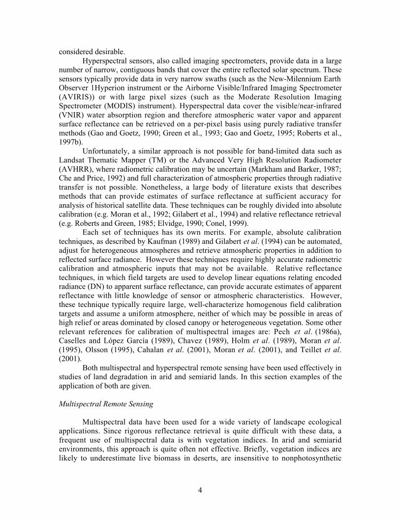
14

Vegetation in more humid environments have largely adapted to maximize theirinterception and absorption of photosynthetically active radiation (PAR). In deserts PARis an over-abundant resource which leads to high temperatures and high evaporativelosses. Therefore, desert vegetation has evolved methods to avoid overheating and loss ofmoisture from evapotranspiration. One way that they accomplish this is to minimize theirsurface areas by reducing leaf size or avoiding leaves altogether and movingphotosynthesis to the stalks and stems. Furthermore, the high densities of reflectivespines on many plants serve not only to protect the soft flesh from predation, but also topartially shade the photosynthetic surface of the plant, to reflect a large proportion ofincoming radiation, and to create a still-air layer around individual segments which canreduce losses to evapotranspiration.

Figure 5. Comparison of spectrum of green vegetation (GV), non-photosyntheticvegetation (NPV) and creosote canopy spectrum. The Best Fit line is the optimal linearleast-squares mixture of GV and NPV to match the creosote spectrum. The residual ofthis mixture (Residual=Creosote Canopy – Best Fit) is given in the bottom panel.

15

Spines and their gentler cousins—leaf hairs—are common features in desert vegetationthat increase the reflectance of vegetation especially in the visible (Ehleringer andMooney, 1978). In addition, because PAR is an over-abundant resource, many desertplants have low concentrations of chlorophyll in their leaves and stems, as exhibited bytheir typically pale green color. The absorption of a photon by chlorophyll generates heat.Having low concentrations of chlorophyll thus helps vegetation further avoidoverheating. Further adaptations include a waxy leaf cuticle that helps reduce losses dueto evapotranspiration. These waxy films often give vegetation anomalous absorptionsaround 1720 nm (Figure 5 and Ray, 1995).

Leaf hairs, spines, and reduced chlorophyll concentration in desert plants all act toreduce leaf absorption in the visible which decreases the red edge in many of these plants.The adaptations of desert plants to their surroundings are largely responses to theradiation environment (intense sun and heat) present in deserts, and thus influencedirectly the spectral characteristics of vegetation. Different plant species have evolveddifferent strategies for coping with the harsh desert environment. The resulting inter-species spectral variability is a consideration in quantitative vegetation remote sensing inarid and semiarid environments because the full range of vegetation spectra must betaken into account. Unfortunately, most types of desert shrubs are not different enoughfrom one another to allow discernment of vegetation type. Okin et al. (2001b) haveshown that even under simplified but realistic best-case conditions, vegetation typecannot be discerned at low covers. Intra-species variability exacerbates this problembecause spectral variability within a species can be greater than variability betweenspecies (Figure 6 and Duncan et al., 1993; Franklin et al., 1993).

Intra-species variability is largely a function of climatic variability in deserts.Precipitation in the world’s arid and semiarid regions is often highly variable in bothspace and time. Desert plants have adapted to this by coordinating their phenologicalstages with the availability of soil moisture. When water becomes available after the dryseason or a period of drought, perennial vegetation will emerge from dormancy, beginphotosynthesis, and if time permits, produce flowers and fruits. When water againbecomes scarce, vegetation will resume dormancy. The total cycle often takes placeduring a relatively short (2-3 month) growing season. Under extended periods of dryness,some vegetation will drop their leaves in “drought deciduous” behavior. Annuals indesert regions also respond opportunistically and rapidly to available soil moisture,

Figure 6. In this striking example of intra-species variability, two adjacent Atriplexpolycarpa bushes exhibit differentphenologies (the bush on the left hasproduced fruit and gone into dormancy, thebush on the right has yet to produceflowers) and therefore different reflectancespectra. (G. Okin, Manix Basin, September13, 1997)

16

sometimes going from germination to fruiting to senescence in a few weeks. Thetemporal variability of vegetation in arid regions contributes to spectral variability withina single region and on smaller scales (Figure 6). No single reflectance spectrum canrepresent the full “spectral phenology” of desert plants and spectra representing differentphenological stages must be incorporated for quantitative information about vegetationchange in both space and time.

SummaryThe retrieval of vegetation parameters from remote sensing presents some

significant challenges:1) Low vegetation cover over bright soils means the vegetation signal can be

swamped out of the pixel-averaged signal,2) Exposed, variable soil surfaces can contribute significantly to within-scene

variability,3) Many remote sensing techniques are insensitive to NPV which can be a

major and important component of total cover in deserts,4) Open canopies and bright soils in desert areas can contribute to significant

multiple scattering and nonlinear mixing in deserts,5) Desert vegetation is spectrally dissimilar to its humid counterparts lacking,

most notably, a strong red edge, and6 ) Rapid phenological changes are accompanied by spectral changes in

desert vegetation which can lead to significant temporal and spatial intra-species spectral variability.

Despite these challenges, it is possible to retrieve quantitative information aboutvegetation remotely as was discussed in the previous section. Nonetheless, in theapplication of remote sensing to problems in desert regions, the limitations andconsiderations discussed here must be anticipated and worked around. Before we turn toa case study of remote sensing in an arid North American shrubland, we will discuss animportant use of remote sensing techniques in desert regions: detection of atmosphericdust.

ATMOSPHERIC REMOTE SENSING IN ARID REGIONS: CLEAR SKY ANDDUSTY DAYS

Atmospherically, arid environments are one of the most hospitable for remotesensing. Many arid regions throughout the globe experience cloudless conditions much ofthe year. This raises the probability that any single pass of an instrument overhead willget a clear view of the surface.

Due in large part to their dryness, however, arid regions are also the world’smajor source of atmospheric mineral aerosols—dust. Mineral aerosols may impact globalclimate through their ability to scatter and absorb light (Sokolik and Toon, 1996) and toaffect cloud properties (Wurzler et al., 2000). Dust is thought to play a major role inocean fertilization and CO2 uptake (Duce and Tindale, 1991; Piketh et al., 2000).Deposition of dust can be important for soil formation and nutrient cycling (Swap et al.,1992; Wells et al., 1995; Reynolds et al., 2001) and serious public health concerns arisein regions affected by high concentrations of atmospheric dust (Griffin et al., 2001).

Dust emission is also a fundamental part of the functioning of arid landscapes.

17

The extent of dust emission has been observed to be a function of many landscape andclimate parameters (for a good review see, Gillette, 1999). Humans impact conditions inthe landscape through land use by removing vegetation and breaking up soil crusts (Okinet al., 2001a). Due to this, some authors have suggested that land use accounts forobserved significant increases in wind erosion in North Africa, the world’s single largestsource of atmospheric dust (Tegen and Fung, 1995; Prospero et al., In Press). Otherinvestigators have suggested that variations in topography and climate can account for thespatial and temporal patterns seen in atmospheric dust using remote sensing (Prospero etal., In Press). Whether natural processes are alone responsible for increases inatmospheric dust concentrations or whether land use also has an impact will remain aquestion for some time to come. In combination with other datasets, remote sensing datawill help address this question.

The remote sensing techniques that can be used to observe atmospheric aerosolscan be divided into 1) those which work over oceans but not land, and 2) those whichwork over both oceans and land. Multispectral sensors that function in the visible are, forthe most part, only valuable for mineral aerosol remote sensing over the oceans. TwoVNIR sensors, AVHRR and the Sea-viewing Wide Field-of-view Sensor (SeaWiFS), arecommonly used to provide information about aerosol optical depth over oceans. Theseinstruments can be used to map atmospheric dust distributions because dust, whenilluminated by the sun, scatters a fraction of the solar radiation back to space (Husar etal., 1997). Over the continents the methods developed for these instruments do not workbecause the radiation scattered by dust is swamped out by that reflected from the surface.Nonetheless, the combination of radiative transfer models and hyperspectral visible/near-infrared data does allow retrieval of aerosol information over the continents for thehyperspectral MODIS instrument (Kaufman et al., 1997; Tanre et al., 1997). Over theoceans, the problem of surface reflectance is minimized and multispectral instrumentscan be used to retrieve aerosol information. The algorithm used to retrieve dustdistributions from AVHRR data uses the backscattered radiance in the 0.63 µm band ofthe instrument and a radiative transfer model that includes idealized mineral aerosols(Husar et al., 1997). Work by Husar et al. (1997) has characterized tropospheric dust overthe oceans, and has revealed many spatially coherent plumes that can be interpreted interms of reasonable sources, with the dust plumes coming off of North Africa andnorthwestern China being prominent features.

Two methods have been developed to measure atmospheric aerosols using non-VNIR methods. The Total Ozone Mapping Spectrometer (TOMS) instrument has a UVspectrometer designed to provide accurate global estimates of total column ozone. Recentdevelopments have shown that it is also capable of estimating both absorbing and non-absorbing aerosols (Figure 7). Herman et al. (1997) have developed at Aerosol Index(AI) derived from TOMS which is defined as:

AI = − −100 10 340 380 10 340 380{log [( / ) ] log [( / ) ]}I I I Imeas calc , (Eq. 6)

where I340 is the radiance 340 nm, I380 is the radiance 380 nm, meas denotes the measuredradiance using the TOMS instrument and calc denotes the radiance calculated using aradiative transfer model that is constructed to give nearly zero AI in the presence ofclouds.

18

Prospero et al. (In Press) have used the TOMS AI index to identify areas that aresources of atmospheric dust on a global scale. By looking at the number of days wherethe AI value was above a pre-determined threshold, Prospero et al. were able to improveour understanding of where, within large desert areas, dust tends to be generated. Theysuggest that dust emission is a spatially varying process that tends to be concentrated inlarge basins where there are ample fine-grained sediments to be eroded. The InfraredDifference Dust Index (IDDI) is derived from images obtained from the Meteosat 10.5µm- to 12.5-µm thermal infrared channel (Chomette et al., 1999). The IDDI is sensitiveto the decrease of the thermal infrared radiance due to the present of dust in theatmosphere during daytime. To compute the IDDI, a time series of geometrically andradiometrically calibrated images are used to create a reference image representingapproximately clear and dust-free conditions. Clouds and dust are separated from thesurface information by subtracting the calibrated images from the reference image andcloudy pixels are masked out. The resulting images provide a time-series of IDDI valuesrelated to atmospheric optical depth.

In an application of the IDDI to understanding the distribution of dust emissionand potentially land degradation in North Africa, Chomette et al. (1999) combined IDDIvalues for North Africa and wind speed at 10-m height to determine threshold windspeed—the wind speed above which wind erosion can occur. This parameter is verysensitive to both surface texture and vegetation cover (Marticorena et al., 1997). Gilletteet al. (1980) have also shown that threshold wind speed is very sensitive to disturbancethrough land use.

The results of the Chomette et al. (1999) and Prospero et al. (In Press) papers

Figure 7. A dust storm coming off the west coast of North Africa on March 6, 1998.The image on the left is a SeaWIFS color composite (www.gsfc.nasa.gov/SEAWIFS/IMAGES/SEAWIFS_GALLERY.html). The image on the left is aTOMS AI image of the same storm (courtesy N. Mahowald). Red are high AI values,blue are low AI values. TOMS AI is defined as: -100{log10[(I340/ I340)meas- log10[(I340/I340)calc]},where I340 is the radiance 340 nm, I380 is the radiance 380 nm, meas denotesthe measured radiance using the TOMS instrument and calc denotes the radiancecalculated using a radiative transfer model that is constructed to give nearly zero AIin the presence of clouds.

19

provides a important basis for work aimed at identifying the spatial locations of desertdust emission as well as the conditions that make these areas particularly susceptible towind erosion. With this information, scientists will be able to evaluate the effect thathumans play in affecting the global dust cycle through the degradation of arid lands.

CASE STUDY: THE MANIX BASIN, SAN BERNARDINO COUNTY,CALIFORNIA

Several techniques that may be used for analysis of remote sensing data in aridregions were discussed in the previous section. In this section, three of thosetechniques—NDVI, SMA, and MESMA—plus a fourth technique—matchedfiltering—will be compared for a single site.

Figure 8. Location of theManix Basin, California.M a p s f r o mwww.nationalatlas.gov.

Figure 9. Landsat TM falsecolor image of the ManixBasin (RGB=542). Interstate15 runs through the center ofthe image and Interstate 40runs through the bottom ofthe image. The Mojave Riverruns from left to right acrossthe image below I-15. Theplaya in the north of theBasin is Coyote Dry Lake.The bright green circles areac t ive cen t ra l p ivo ta g r i c u l t u r e . S e v e r a labandoned fields can also beseen throughout the Basin,particularly in the North.TM image from the MojaveDesert Ecosystem Project.

20

The Manix Basin is in the Mojave Desert, about 25 miles ENE of Barstow insoutheastern California (centered around 34°56.5’ N 116°41.5’ W at an elevation ofabout 540 m) (Figure 8). The basin has an area of 40,700 ha and was the site of ancientLake Manix which existed during the peak pluvial episode of the last glaciation anddrained through Afton Canyon to the east (Smith and Street-Perrott, 1983; Meek, 1989).Much of the basin is filled with lacustrine, fluvial, and deltaic sediments capped by weakarmoring (Meek, 1990). There is clear evidence of pre-modern wind erosion, indicatingthat wind erosion, transport, and deposition has long been a dominant geological processin the area (Evans, 1962).

The modern climate of the Manix Basin is arid with the average annualprecipitation of 10 cm falling mostly in the winter, although there can be significantsummer precipitation in some years (Okin et al., 2001a). The average annual temperatureis 19.6°C, the average winter temperature is 9.1°C, and the average summer temperatureis 31.4°C (Meek, 1990). The vegetation in undisturbed areas of the basin is dominated byan association of Larrea tridentata and Ambrosia dumosa with minor occurrence ofAtriplex polycarpa, Atriplex hymenelytra, Atriplex canescens, Ephedra californica, andOpuntia spp. Prosopis glandulosa occurs in some areas of the basin. Vegetation cover inundisturbed areas rarely exceeds (10%) (Okin et al., 2001a). Areas that have beendisturbed directly by human activity are dominated by At. polycarpa with total coveroften greater than that in undisturbed desert (~30%). Schismus, an exotic annual grass, isubiquitous, but grass cover varies significantly with yearly precipitation.

Human activity in the Manix Basin (Figure 9) has been extensive, with severalphases of agricultural activity utilizing groundwater recharged by the Mojave River,which carries runoff from the San Bernardino Mountains to the south-southwest (Tugeland Woodruff, 1978). The basin was used for dryland farming in the 1800s (Tugel andWoodruff, 1978). Limited irrigated farming started in the basin in 1902 with the acreageof irrigated land increasing sharply after World War II (Tugel and Woodruff, 1978).Today alfalfa hay is the major agricultural product. In the Coyote Dry Lake sub-basin,square flood-irrigated fields and abandoned flood irrigation equipment are seen in earlyLandsat images. After the mid-1970s, central-pivot agriculture became the dominantform of land use in the area, but many fields have now been abandoned throughout thenorthern part of the basin due to increasing costs of pumping groundwater to the surfacefor agriculture (Ray, 1995).

AVIRIS data were acquired over the Manix Basin on April 30, 1998. Thenorthern lobe of the Manix Basin is the focus of this study and is covered by flight980430 run 10 scene 3 (Figure 10). The data were radiometrically calibrated at theAVIRIS data facility (Jet Propulsion Laboratory, Pasadena, California). Apparent surfacereflectance was retrieved using a technique developed by Green et al. (Green et al., 1993;Green et al., 1996; Roberts et al., 1997b). The reflectance spectrum from a gravel parkinglot in the scene was used to correct the apparent surface reflectance spectra of the entirescene (Clark et al., 1995). The products derived from the AVIRIS image were rectifiedusing a nearest-neighbor triangulation method that employed 107 ground-control pointschosen in the image and in a series of 1-m resolution USGS digital orthophotos.

21

Landsat TM data from the Mojave Desert Ecosystem Project (MDEP) were usedto create NDVI images for the area colocated with the April 30, 1998 AVIRIS image(Figure 11). The NDVI values for the image on the left in Figure 11, which has not beenstretched to enhance contrast within the area of interest, shows the low response of NDVIto the vegetation in the Basin. This is largely due to the fact that NDVI is insensitive toNPV which dominates vegetation cover in the area. The generally low NDVI values inthe Basin are thus due to the low cover generally as well as the relatively low proportionof GV to NPV. In the contrast-enhanced image on the left, it is evident that NDVI isrelatively high for two areas that have high cover of At. polycarpa: B and C. Area A,however, also has relatively high NDVI values, but these two abandoned fields lackvegetation cover completely. Here, the high NDVI value relative to the surroundingundisturbed desert, is likely due to a change in soil color associated with tillage of thesefields. In addition, the northernmost small playa on the right edge of the image displayshigh NDVI values. This playa has no vegetation cover.

Figure 10. Landsat TMimage (RGB=542) of thenorthern part of the ManixBasin. Letters denote featuresin the basin discussed in thetext. The heavy blackrectangle in the imagedenotes the extent of theAVIRIS image discussed inthe text.

22

Despite these discrepancies between NDVI values and actual cover in the Basin,there is relatively good agreement between the NDVI image and the MESMA-derivedvegetation (GV + NPV) cover map (Figure 12). Both MESMA and NDVI vegetationgenerally decrease from south to north and west to east in the image, with nearly zerocover close to Coyote Dry Lake (H), on the relic beach terrace in the northern part of thebasin (I), on the wash on the left corner of the image, on Agate Hill (G) and on alluvial

Figure 11. NDVI image of the study area in the Manix Basin.. The image on theleft has been scaled so that black is essentially no vegetation and white is the valueof riparian vegetation with nearly 100% cover (in an area not colocated with theAVIRIS image). The image on the right has been stretched to enhance the contrastwithin the bounds of the AVIRIS image.

Figure 12. MESMA-derived mapof soil and vegetation cover in theAVIRIS image. This figure is theproduct of 1,885 four-endmembermodels utilizing ground spectra ofshrubs, grasses (senesced), andsoils from the Manix Basin.White areas are places where nomodel was fit within theconstraints. For more informationsee, Okin et al. (2001b).

23

fan #2. MESMA and NDVI disagree on the relative amounts of vegetation cover onabandoned fields A, E, and F, on the grounds of St. Francis Monastery (D), and onalluvial fan #1. In general, the vegetation cover map based on MESMA represents mostclosely the degree of cover in this part of the basin (G.S. Okin, personal observations, andOkin et al., 2001a).

Many discrepancies exist in comparing the MESMA-derived vegetation covermap with that from simple unmixing (SMA) (Figure 13). As with NDVI, SMAoverestimates the degree of vegetation on the bare abandoned fields A, E, and F, and onthe grounds of the Monastery (G). On abandoned fields B and C, SMA does identify thepresence of significant vegetation, but the rightmost field in B is modeled as having alarge amount of GV. This is also seen in the northern part of the image (H and I) whichaccording to MESMA, NDVI, and field observations has low cover. Under SMA, thisarea is modeled as nearly 100% GV cover. Indeed, SMA fails to display the same patternof vegetation cover in undisturbed areas seen in both MESMA and NDVI (coverdecreasing from left to right and bottom to top across the image). Furthermore, SMAfails to identify the plume of vegetation cover downwind of the abandoned fields, B. Thisplume is located on bright wind-blown soils derived from the abandoned fields and can

be covered quite heavily by Schismus grass during wet years such as 1998.Many of the problems with SMA in the current case study can be traced to the

variability of soils in the Basin. For instance, the soils in the north (H) are sandy soils thatare spectrally distinct from the armored soils of the rest of the Basin floor and used in theSMA model. This leads to dramatic overestimation of green vegetation in these areas.The disturbed soils of A, E, F, and G also display overestimations in total cover in theseareas probably due to the deviation of the soil spectra here from that used in the SMAmodel.

In general, due to inflexibility in the soil endmember in this highly variablelandscape, SMA yields the poorest results of the three methods in identifying patterns of

Figure 13. Simple unmixing(SMA)-derived map of soil andvegetation cover in the AVIRISimage calculated using GV(Poplar leaf), NPV (dry grass),and a field spectrum of soil fromwithin the basin (see Figure 5 forvegetation spectra). Areasappearing white in the image aremodeled by SMA as havinganomalously high amounts of GV(approaching 100%).

24

vegetation cover in the Manix Basin although this can depend on the endmember used.NDVI, while capturing some of the basic patterns in the image, yields many inaccuracies,particularly in areas where the soils have been disturbed by land use. These discrepanciescan be largely attributed to variations in soil color and the insensitivity of NDVI to NPVwhich dominates the vegetation cover in the image. Only MESMA, which canaccommodate variability in both the soil and vegetation endmembers yields believablevegetation cover results.

Okin et al. (2001b) have also shown that MESMA is able to correctly identifysurface soil type (sandy soils from armored soils) in the Basin. Their analysis, however,indicates that MESMA is not able to correctly discriminate between vegetation typesbelow at least 30% cover. They conclude that many other techniques that use subtlespectral differences to differentiate between like materials (such as spectral matching)will also be unable to discriminate between vegetation types under these conditions.

Despite the difficulty of using many standard remote sensing techniques in aridregions, current research is exploring new avenues for vegetation detection. One methodwhich is currently being considered is matched filtering, a technique that was developedto detect extremely weak signals that are essentially in the noise. Unlike SMA, MESMA,and spectral matching, matched filtering is optimized to detect extremely weak signals(for a good review see Funk et al., 2001) and therefore may be able to discriminatebetween vegetation types in arid regions. Matched filtering works by separatinghyperspectral reflectance into “signal” and “noise” components. The signal is the desiredspectrum scaled to represent its radiance in a pixel. Everything else is assumed to benoise. Matched filtering returns σ-values which denote the number of standarddeviations a given pixel’s matched filter score is from zero. Large positive sigma valuesindicate high likelihood that a signal is present in a pixel.

Using matched filtering to try to identify the distributions of various vegetationtypes within the Manix Basin yields promising results (Figure 14) when compared toobservations of vegetation distribution in the area (G.S. Okin, personal observations, andOkin et al., 2001a). The dominance of At. polycarpa and senesced grass on the right side

Figure 14. Matched filter results fromthe Manix AVIRIS scene. The redchannel σ -values for senescedSchismus grass. The green channel isσ-values for L. tridentata. The bluechannel is σ-values for At. polycarpa.

25

of B, for instance, agrees with the dominance of these cover types there. The dominanceof L. tridentata and senesced grass in the undisturbed portions of the Basin is consistentwith observations. The dominance of senesced grass on D, E, in the vicinity of I, anddownwind of A is also consistent with observations. But the results are far from perfect.Some areas of no cover in the basin (A and the bare playas) falsely indicate the presenceof L. tridentata and the two white areas strongly show the presence of all three vegetationtypes, which is unrealistic in this situation.

The use of advanced spectral techniques to discriminate vegetation type in aridareas remains the subject of ongoing research. The matched filter example here providesinsight into the cutting edge to solving this significant technical hurdle.

SUMMARYRemote sensing is a cost- and time-efficient way to determine the spatial

characteristics of desert-derived mineral aerosols, desert soils and vegetation, and landuse and land degradation in arid regions. Several robust techniques exist to estimate theconcentration of mineral aerosols over both the oceans and continents. Further use ofthese data along with ground data will help to constrain the global sources and impacts ofdesert dust.

The use of remote sensing to understand land use and land degradation is acommon goal in modern research. Nonetheless, special complications are presentedwhen using remote sensing to look at soils and vegetation in deserts. These arise from thesparse vegetation cover, spectrally unique vegetation, and bright soils common to aridregions and cannot be taken for granted. As the example from the Manix Basin shows,the use vegetation indices, while easy to calculate and conceptually simple, can bedangerous: they provide deceiving results which may be correct in one part of an imageand seriously flawed nearby. Other spectral techniques such as SMA show promise inmapping vegetation cover, and the SMA-superset, MESMA, is by far the most robustspectral analysis technique for use in arid regions. Given both the challenges andpromises of remote sensing in deserts, research continues in the use of remote sensing todetect process-relevant surface parameters.

BIBLIOGRAPHYAdams J. B., Smith M. O., and Gillespie A. R. (1993), Remote Geochemical Analysis: Elemental and

Mineralogical Composition (C. M. Pieters and P. A. J. EnglertEds.), Cambridge University Press,Cambridge, pp. Ch. 7.

Bailey T. C., and Gatrell A. C. (1995), Interactice Spatial Data Analysis. Addison Wesley LongmanLimited, Essex, England.

Billings W. D., and Morris R. J. (1951), Reflection of visible and infrared radiation for leaves of differentecological groups. American Journal of Botany. 39: 327-331.

Buffington L. C., and Herbel C. H. (1965), Vegetational changes on a semidesert grassland range from1858 to 1963. Ecological Monographs. 35: 139-164.

Cahalan R. F., Oreopoulos L., Wen G., Marshak A., Tsay S. C., and DeFelice T. (2001), Cloudcharacterization and clear-sky correction from Landsat-7. Remote Sensing of Environment. 78: 83-98.

Caselles V., and Garcia M. J. L. (1989), An alternative simple approach to estimate atmospheric correctionin multitemporal studies. International Journal of Remote Sensing. 10: 1127-1134.

Chavez P. R., Jr. (1989), Radiometric calibration of Landsat Thematic Mapper multispectral images.Photogrammetric Engineering and Remote Sensing. 55: 1285-1294.

Che N., and Price J. C. (1992), Survey of radiometric calibration results and methods for visible and near-infrared channels of NOAA-7, NOAA-9, and NOAA- 11 AVHRRs. Remote Sensing of Environment.

26

41: 19-27.Chen Z., Elvidge C. D., and Groeneveld D. P. (1998), Monitoring seasonal dynamics of arid land

vegetation using AVIRIS data. Remote Sensing of Environment. 65: 255-266.Chilès J.-P., and Delfiner P. (1999), Geostatistics. John Wiley and Sons, Inc., New York.Chomette O., Legrand M., and Marticorena B. (1999), Determination of the wind speed threshold for the

emission of desert dust using satellite remote sensing in the thermal infrared. Journal of GeophysicalResearch. 104: 31207-31215.

Clark R. N. (1997), Spectroscopy of Rocks and Minerals, and Principles of Spectroscopy. In Manual ofRemote Sensing (A. Rencz. Ed.), John Wiley and Sons, Inc., pp. Chapter 1.

Clark R. N., Swayze G. A., and Heidebrecht K. (1995), Calibration to surface reflectance of terrestrialimaging spectrometry data: Comparison of methods. Summaries of the Fifth Annual JPL AirborneEarth Science Workshop, Jet Propulsion Laboratory, Pasadena, CA, 41-42.

Conel J. E. (1999), Determination of surface reflectance and estimates of atmospheric optical depth andsingle scattering albedo from Landsat Thematic Mapper. International Journal of Remote Sensing. 11:783-828.

Drake N. A., Mackin S., and Settle J. J. (1999), Mapping vegetation, soils, and geology in semiaridshrublands using spectral matching and mixture modeling of SWIR AVIRIS imagery. Remote Sensingof Environment. 68: 12-25.

Duce R. A., and Tindale N. W. (1991), Atmospheric transport of iron and its deposition in the ocean.Limnology and Oceanography. 36: 1715-1726.

Duncan J., Stow D., Franklin J., and Hope A. (1993), Assessing the relationship between spectralvegetation indices and shrub cover in the Jornada Basin, New Mexico. International Journal of RemoteSensing. 14: 3395-3416.

Ehleringer J. (1981), Leaf absorptances of Mohave and Sonoran Desert plants. Oecologia. 49: 366-370.Ehleringer J., and Björkman O. (1976), Leaf pubescence: effects on absorptance and photosynthesis in a

desert shrub. Science. 192: 376-377.Ehleringer J. R., and Björkman O. (1978), Pubescence and leaf spectral characteristics in a desert shrub,

Encilia farinosa. Oecologia. 36: 151-162.Ehleringer J. R., and Mooney H. A. (1978), Leaf hairs: effects on physiological activity and adaptive value

to a desert shrub. Oecologia. 37: 183-200.Elmore A. J., Mustard J. F., Manning S. J., and Lobell D. B. (2000), Quantifying vegetation change in

semiarid environments: Precision and accuracy of spectral mixture analysis and the NormalizedDifference Vegetation Index. Remote Sensing of Environment. 73: 87-102.

Elvidge C. D. (1990), Visible and near-infrared reflectance characteristics of dry plant materials.International Journal of Remote Sensing. 11: 1775-1795.

Elvidge C. D., Chen Z., and Groeneveld D. P. (1993), Detection of trace quantities of green vegetation in1990 AVIRIS data. Remote Sensing of Environment. 44: 271-279.

Escafadel R., and Huete A. R. (1991), Improvement in remote sensing of low vegetation cover in aridregions by correcting vegetation indices for soil "noise". C. R. Academie des Sciences Paris. 312:1385-1391.

Evans J. R. (1962), Falling and climbing sand dunes in the Cronese ("Cat") Mountain Area, San BernardinoCounty, California. Journal of Geology. 70: 107-113.

Franklin J., Duncan J., and Turner D. L. (1993), Reflectance of vegetation and soil in Chihuahuan desertplant communities from ground radiometry using SPOT wavebands. Remote Sensing of Environment.46: 291-304.

Franklin J., and Turner D. L. (1992), The application of a geometric optical canopy reflectance model tosemiarid shrub vegetation. IEEE Transactions on Geoscience and Remote Sensing. 30: 293-301.

Funk C. C., Theiler J., Roberts D. A., and Borel C. C. (2001), Clustering to improve matched filterdetection of weak gas plumes in hyperspectral thermal imagery. IEEE Transactions on Geoscience andRemote Sensing. 39: 1410-1420.

Gao B.-C., and Goetz A. F. H. (1990), Column atmospheric water vapor and vegetation liquid waterretrievals from airborne imaging spectrometer data. Journal of Geophysical Research. 95: 3549-3564.

Gao B. C., and Goetz A. F. H. (1995), Retrieval of equivalent water thickness and information related tobiochemical-components of vegetation canopies from AVIRIS data. Remote Sensing of Environment.52: 155-162.

García-Haro F. J., Gilabert M. A., and Meliám J. (1996), Linear spectral mixture modelling to estimate

27

vegetation amount from optical spectral data. International Journal of Remote Sensing. 17: 3373-3400.Garcia-Pichel F., and Belnap J. (1996), Microenvironments and microscale productivity of cyanobacterial

desert crusts. Journal of Phycology. 32: 774-782.Gardner M. (1997), Mapping Chaparral with AVIRIS Using Advanced Remote Sensing Techniques. M.A.

Thesis, University of California.Gates D. M., Keegan H. J., Schleter J. C., and Weidner V. R. (1965), Spectral properties of plants. Applied

Optics. 4: 11-20.Gilabert M. A., Conese C., and Maselli F. (1994), An atmospheric correction method for the automatic

retrieval of surface reflectances from TM images. International Journal of Remote Sensing. 15: 2065-2086.

Gilabert M. A., García-Haro F. J., and Melia J. (2000), A mixture modeling approach to estimatevegetation parameters for heterogeneous canopies in remote sensing. Remote Sensing of Environment.72: 328-345.

Gillespie A. R., Smith M. O., Adams J. B., Willis S. C., Fischer A. F., III, and Sabol D. E., Jr. (1990),Interpretation of residual images: Spectral mixture analysis of AVIRIS images, Owens Valley,California. Second AVIRIS Workshop, Jet Propulsion Laboratory, Pasadena, California, 243-270.

Gillette D. A. (1999), A qualitative geophysical explanation for "hot spot" dust emission source regions.Contributions to Atmospheric Physics. 72: 67-77.

Gillette D. A., Adams J., Endo A., Smith D., and Kihl R. (1980), Threshold velocities for input of soilparticles into the air by desert soils. Journal of Geographical Research. 85: 5621-5630.

Graetz R. D., and Gentle M. R. (1982), The relationships between reflectance in the Landsat wavebandsand the composition of an Australian semi-arid shrub rangeland. Photogrammetric Engineering andRemote Sensing. 48: 1721-1730.

Graetz R. D., Pech R. P., and Davis A. W. (1988), The assessment and monitoring of sparsely vegetatedrangelands using calibrated Landsat data. International Journal of Remote Sensing. 9: 1201-1222.

Green R. O., Conel J. E., and Roberts D. A. (1993), Estimation of aerosol optical depth and additionalatmospheric parameters for the calculation of apparent surface reflectance from radiance measured bythe Airborne Visible/Infrared Imaging Spectrometer. Fourth Annual JPL Airborne GeoscienceWorkshop, Pasadena, CA, 73-76.

Green R. O., Roberts D. A., and Conel J. E. (1996), Characterization and compensation of the atmospherefor the inversion of AVIRIS calibrated radiance to apparent surface reflectance. Sixth Annual JPLAirborne Earth Science Workshop, Pasadena, CA, 135-146.

Griffin D. W., Garrison V. H., Herman J. R., and Shinn E. A. (2001), African desert dust in the Caribbeanatmosphere: Microbiology and public health. Aerobiologia. 17: 203-213.

Hall F. G., Shimabukuro Y. E., and Huemmrich K. F. (1995), Remote sensing of forest biophysicalstructure using mixture decomposition and geometric reflectance models. Ecological Applications. 5:993-1013.

Herman J. R., Bhartia P. K., Torres O., Hsu C., Seftor C., and Celarier E. (1997), Global distribution ofUV-absorbing aerosols from Nimbus 7/TOMS data. Journal of Geophysical Research. 102: 16911-16922.

Holm R. G., Jackson R. D., Yuan B., Moran M. S., Slater P. N., and Biggar S. F. (1989), Surfacereflectance factor retrieval from Thematic Mapper data. Remote Sensing of Environment. 27: 47-57.

Hudak A. T., and Wessman C. A. (1998), Textural analysis of historical aerial photography to characterizewoody plant encroachment in South African savanna. Remote Sensing of Environment. 66: 317-330.

Huete A. R. (1988), A soil-adjusted vegetation index (SAVI). Remote Sensing of Environment. 25: 295-309.

Huete A. R., and Jackson R. D. (1987), Suitability of spectral indices for evaluating vegetationcharacteristics on arid rangelands. Remote Sensing of Environment. 23: 213-232.

Huete A. R., and Jackson R. D. (1988), Soil and atmosphere influences on the spectra of partial canopies.Remote Sensing of Environment. 25: 89-105.

Huete A. R., Jackson R. D., and Post D. F. (1985), Spectral response of a plant canopy with different soilbackgrounds. Remote Sensing of Environment. 17: 37-53.

Huete A. R., and Tucker C. J. (1991), Investigation of soil influences in ABHRR red and near-infraredvegetation index imagery. International Journal of Remote Sensing. 12: 1223-1242.

Hurcom S. J., and Harrison A. R. (1998), The NDVI and spectral decomposition for semi-arid vegetationabundance estimation. International Journal of Remote Sensing. 19: 3109-3125.

28

Husar R. B., Prospero J. M., and Stowe L. L. (1997), Characterization of tropospheric aerosols over theoceans with the NOAA advanced very high resolution radiometer optical thickness operationalproduct. Journal of Geophysical Research. 102: 16889-16909.

Jeltsch F., Milton S. J., Dean W. R. J., and van Rooyen N. (1997), Simulated pattern formation aroundartificial waterholes in the semi-arid Kalahari. Journal of Applied Ecology. 8: 177-188.

Kaufman Y. J. (1989), Theory and Applications of Optical Remote Sensing (G. Asrar, Ed.), John Wiley andSons, New York, pp. Chapter 9.

Kaufman Y. J., Tanre D., Remer L. A., Vermote E. F., Chu A., and Holben B. N. (1997), Operationalremote sensing of tropospheric aerosol over land from EOS moderate resolution imagingspectroradiometer. Journal of Geophysical Research-Atmospheres. 102: 17051-17067.

Koch M., and El Baz F. (1998), Identifying the effects of the Gulf War on the geomorphic features ofKuwait by remote sensing and GIS. Photogrammetric Engineering and Remote Sensing. 64: 739-747.

Lancaster N., and Baas A. (1998), Influence of vegetation cover on sand transportation by wind: Fieldstudies at Owens Lake, California. Earth Surface Processes and Landforms. 23: 69-82.

Lange R. T. (1969), The piosphere: sheep track and dung patterns. Journal of Range Management. 22: 396-400.

Markham B. L., and Barker J. L. (1987), Radiometric Properties of U.S. processed Landsat MSS data.Remote Sensing of Environment. 22: 39-71.

Marticorena B., Bergametti G., Gillette D. A., and Belnap J. (1997), Factors controlling threshold frictionvelocity in semiarid and arid areas of the United States. Journal of Geophysical Research. 102: 23277-23287.

McGwire K., Minor T., and Fenstermaker L. (2000), Hyperspectral mixture modeling for quantifyingsparse vegetation cover in arid environments. Remote Sensing of Environment. 72: 360-374.

Meek N. (1989), Geomorphic and hydrologic implications of the rapid incision of Afton Canyon, MojaveDesert, California. Geology. 17: 7-10.

Meek N. (1990), Late Quaternary Geochronology and Geomorphology of the Manix Basin, San BernardinoCounty, California. Ph.D., University of California at Los Angeles.

Mooney H. A., Ehleringer J., and Björkman O. (1977), The energy balance of leaves of the evergreendesert shrub Atriplex hymenelytra. Oecologia. 29: 301-310.

Moran M. S., Bryant R., Thome K., Ni W., Nouvellon Y., Gonzalez-Dugo M. P., and Qi J. (2001), Arefined empirical line approach for reflectance factor retrieval from Landsat-5 TM and Landsat-7ETM+. Remote Sensing of Environment. 78: 71-82.

Moran M. S., Jackson R. D., Clarke T. R., Qi J., Cabot F., Thome K. J., and Markham B. L. (1995),Reflectance factor retrieval from Landsat TM and Spot HRV data for bright and dark targets. RemoteSensing of Environment. 52: 218-230.

Moran M. S., Jackson R. D., Slater P. N., and Teillet P. M. (1992), Evaluation of simplified procedures forretrieval of land surface reflectance factors from satellite sensor output. Remote Sensing ofEnvironment. 41: 169-184.

Muhs D. R., and Maat P. B. (1993), The potential response of eolian sands to greenhouse warming andprecipitation reduction on the Great Plains of the USA. Journal of Arid Environments. 25: 351-361.

Okin G. S., and Gillette D. A. (2001), Distribution of vegetation in wind-dominated landscapes:Implications for wind erosion modeling and landscape processes. Journal of Geophysical Research.106: 9673-9683.

Okin G. S., Murray B., and Schlesinger W. H. (2001a), Degradation of sandy arid shrubland environments:observations, process modelling, and management implications. Journal of Arid Environments. 47:123-144.

Okin G. S., Okin W. J., Murray B., and Roberts D. A. (2001b), Practical limits on hyperspectral vegetationdiscrimination in arid and semiarid environments. Remote Sensing of Environment. 77: 212-225.

Olsson H. (1995), Reflectance Calibration of Thematic Mapper Data for Forest Change Detection.International Journal of Remote Sensing. 16: 81-96.

Pech R. P., and Davis A. W. (1987), Reflectance modeling of semiarid woodlands. Remote Sensing ofEnvironment. 23: 365-377.

Pech R. P., Davis A. W., Lamacraft R. R., and Graetz R. D. (1986a), Calibration of Landsat data forsparsely vegetated semiarid rangelands. International Journal of Remote Sensing. 7: 1729-1750.

Pech R. P., Graetz R. D., and Davis A. W. (1986b), Reflectance modeling and the derivation of vegetationindexes for an Australian semiarid shrubland. International Journal of Remote Sensing. 7: 389-403.

29

Peddle D. R., Hall F. G., and LeDrew E. F. (1999), Spectral mixture analysis and geometric-opticalreflectance modeling of boreal forest biophysical structure. Remote Sensing of Environment. 67: 288-297.

Peters A. J., and Eve M. D. (1995), Satellite monitoring of desert plant community response to moistureavailability. Environmental Monitoring and Assessment. 37: 273-287.

Phinn S., Franklin J., Hope A., Stow D., and Huenneke L. (1996), Biomass distribution mapping usingairborne digital video imagery and spatial statistics in a semi-arid environment. Journal ofEnvironmental Management. 47: 139-164.

Pickup G., and Chewings V. H. (1994), A grazing-gradient approach to land degradation assessment in aridareas from remotely-sensed data. International Journal of Remote Sensing. 15: 597-617.

Piketh S. J., Tyson P. D., and Steffen W. (2000), Aeolian transport from southern Africa and ironfertilization of marine biota in the South Indian Ocean. South African Journal of Geology. 96: 244-246.

Prospero J. M., Ginoux P., Torres O., and Nicholson S. E. (In Press), Environmental characterization ofglobal sources of atmospheric soil dust derived from the NIMBUS-7 absorbing aerosol product.Reviews of Geophysics.

Ray T. W. (1995), Remote Monitoring of Land Degradation in Arid/Semiarid Regions. Ph.D., CaliforniaInstitute of Technology.

Ray T. W., and Murray B. C. (1996), Nonlinear spectral mixing in desert vegetation. Remote Sensing ofEnvironment. 55: 59-64.

Reynolds R., Belnap J., Reheis M., Lamothe P., and Luiszer F. (2001), Aeolian dust in Colorado Plateausoils: Nutrient inputs and recent change in source. Proceedings of the National Academy of Sciences ofthe United States of America. 98: 7123-7127.

Roberts D. A., Adams J. B., and Smith M. O. (1990), Predicted distribution of visible and near-infraredradiant-flux above and below a transmittant leaf. Remote Sensing of Environment. 34: 1-17.

Roberts D. A., Gardner M., Church R., Ustin S., Scheer G., and Green R. O. (1998), Mapping chaparral inthe Santa Monica Mountains using multiple endmember spectral mixture models. Remote Sensing ofEnvironment. 65: 267-279.

Roberts D. A., Gardner M., Church R., Ustin S. L., and Green R. O. (1997a), Optimum strategies formapping vegetation using multiple endmember spectral mixture models. SPIE Conference ImagingSpectrometry III, San Diego, CA, 108-119.

Roberts D. A., and Green R. O. (1985), Detection of hydrocarbon microseeps and relatedgeobotanical anomalies using multi-date image subtraction, Railroad Valley, Nevada. Proceedings of the

19th International Symposium on Remote Sensing of Environment, Ann Arbor, Michigan.Roberts D. A., Green R. O., and Adams J. B. (1997b), Temporal and spatial patterns in vegetation and

atmospheric properties from AVIRIS. Remote Sensing of Environment. 62: 223-240.Roberts D. A., Smith M. O., and Adams J. B. (1993), Green vegetation, nonphotosynthetic vegetation, and

soils in AVIRIS data. Remote Sensing of Environment. 44: 255-269.Robinove C. J., Chavez P. S., Jr., Gehring D., and Holmgren R. (1981), Arid land monitoring using Landsat

albedo difference images. Remote Sensing of Environment. 11: 133-156.Schlesinger W. H., Raikes J. A., Hartley A. E., and Cross A. F. (1996), On the spatial pattern of soil

nutrients in desert ecosystems. Ecology. 77: 364-374.Schlesinger W. H., Reynolds J. F., Cunningham G. L., Huenneke L. F., Jarrell W. M., Virginia R. A., and

Whitford W. G. (1990), Biological feedbacks in global desertification. Science. 247: 1043-1048.Schultz B. W., and Ostler W. K. (1993), Effects of prolonged drought on vegetation association in the

Northern Mojave Desert. Wildland shrubs and arid land restoration symposium, Las Vegas, Nevada,228-235.

Settle J. J., and Drake N. A. (1993), Linear mixing and the estimation of ground cover proportions.International Journal of Remote Sensing. 14: 1159-1177.

Shimabukuro Y. E., and Smith J. A. (1991), The least-squares mixing models to generate fraction imagesderived from remote sensing multispectral data. IEEE Transactions on Geoscience and RemoteSensing. N1: 16-20.

Smith G. I., and Street-Perrott F. A. (1983), Pluvial Lakes of the Western United States. In LateQuaternary Environments of the United States, Vol. 1 (H. E. Wright, Jr._Ed., University of MinnesotaPress, Minneapolis, Minnesota, pp. 190-212.

Smith M. O., Ustin S. L., Adams J. B., and Gillespie A. R. (1990), Vegetation in deserts: I. a regionalmeasure of abundance from multispectral images. Remote Sensing of Environment. 31: 1-26.

30

Sokolik I. N., and Toon O. B. (1996), Direct radiative forcing by anthropogenic airborne mineral aerosols.Nature. 381: 681-683.

Swap R., Garstang M., Greco S., Talbot R., and Kallberg P. (1992), Saharan dust in the Amazon Basin.Tellus Series B-Chemical and Physical Meteorology. 44: 133-149.

Tanre D., Kaufman Y. J., Herman M., and Mattoo S. (1997), Remote sensing of aerosol properties overoceans using the MODIS/EOS spectral radiances. Journal of Geophysical Research-Atmospheres. 102:16971-16988.

Tegen I., and Fung I. (1995), Contribution to the atmospheric mineral aerosol load from land surfacemodification. Journal of Geophysical Research. 100: 18707-18726.

Teillet P. M., Barker J. L., Markham B. L., Irish R. R., Fedosejevs G., and Storey J. C. (2001), Radiometriccross-calibration of the Landsat-7 ETM+ and Landsat-5 TM sensors based on tandem data sets.Remote Sensing of Environment. 78: 39-54.

Tsoar H., and Karnieli A. (1996), What determines the spectral reflectance of the Negev-Sinai sand dunes.International Journal of Remote Sensing. 17: 513-525.

Tucker C. J., Dregne H. E., and Newcomb W. W. (1991), Expansion and contraction of the Sahara Desertfrom 1980 to 1990. Science. 253: 299-301.

Tucker C. J., Newcomb W. W., and Dregne H. E. (1994), AVHRR data sets for determination of desertspatial extent. International Journal of Remote Sensing. 15: 3547-3565.

Tugel A. J., and Woodruff G. A. (1978), Soil Survey of San Bernardino County, California: Mojave RiverArea. Soil Conservation Service, United States Department of Agriculture.

Ustin S. L., Adams J. B., Elvidge C. D., Rejmanek M., Rock B. N., Smith M. O., Thomas R. W., andWoodward R. A. (1986), Thematic Mapper studies of semiarid shrub communities. BioScience. 36:446-452.

Wells S. G., McFadden L. D., Poths J., and Olinger C. T. (1995), Cosmogenic 3He surface-exposure datingof stone pavements: implications for landscape evolution in deserts. Geology. 23: 613-616.

Wiggs G. F. S., Thomas D. S. G., and Bullard J. E. (1995), Dune mobility and vegetation cover in thesouthwest Kalahari Desert. Earth Surface Processes and Landforms. 20: 515-529.

Wurzler S., Reisin T. G., and Levin Z. (2000), Modification of mineral dust particles by cloud processingand subsequent effects on drop size distributions. Journal of Geophysical Research. 105: 4501-4512.