reml estimation and linear mixed models 3. analysis of

1

REML Estimation and Linear Mixed Models

3. Analysis of longitudinal data

Sue Welham

Rothamsted ResearchHarpenden UK AL5 2JQ

November 18, 2008

Introduction

Introduction

Balanced repeatedmeasurements

Unbalanced repeatedmeasurements

2

Longitudinal data is data arising from several measurements made on a set ofsubjects over time.

The amount of structure in the data varies between two extreme cases:

■ Balanced repeated measurements: treatments are allocated to subjects as adesigned experiment, these remain constant throughout the study andmeasurements are made on all subjects at a common set of time-points

■ Observational data: subjects are observed at certain intervals over time.Each subject may be measured a different number of times, at differentintervals to other subjects. There may be many background covariates thathave to be accounted for, which may change over time and will usually notbe independent (collinearity) and will often be confounded with thecovariates of interest.

More typically, a data set might consist of experimental data, with treatmentsallocated (possibly changing) according to a pre-planned design, which is not quitebalanced and with some additional background covariates to account for.

We will look initially at the balanced case and then consider unbalanced data.

Missing data

Introduction



3

One important aspect of longitudinal data is the status of missing data: this bemissing and uninformative:

■ a scientist forgot to measure a plant

■ a patient forgot to turn up for an assessment

but may be informative:

■ the allocated treatment killed the plant

■ the allocated treatment made the patient too sick to attend the assessment

Much work has been done on the analysis of missing data in longitudinal studies(see eg Verbeke & Molenberghs, 2000) but this will not be covered here.

Aims of analysis

Introduction



4

■ In longitudinal data/ repeated measurements, the aim is usually to modelcovariance across times within subjects in order to get better estimates oftreatment effects and SEDs

■ Efficient identification of a important fixed terms is usually the primaryobjective

■ But identification of a good variance model can aid this process - this is ourfocus

■ We will consider two approaches to this:

◆ modelling the covariance structure directly using different covariancestructures

◆ modelling the covariance structure indirectly via random coefficientregression

Simple ANOVA model

Introduction


ANOVA model

General mixed model

Example

AR model

Composite models

Het. AR model

Ante-dependence

AIC & BIC

Model selection

Alternative approach


5

General form of data:

■ p replicates of g treatments allocated to N = pg subjects as a designedexperiment (may include blocking)

■ repeated measurements made on subjects at r time points t = (t1 . . . tr)′

Returning to Brien & Bailey method of model determination (assume no blocking):

Tier 2 Tier 1Treatment → SubjectTime 99K Measurement w/i Subjects

99K indicates that times cannot be randomized: time 1 always comes first

■ Simplest model

yij = µ+ Tv + βj + (Tβ)vj + si + eij

◆ yij is measurement on subject i (i = 1 . . . N) at time j (j = 1 . . . r)

◆ v = v(i) is the treatment allocated to subject i

◆ Tk fixed effect of treatment k, βj fixed effect of measurement time j,(Tβ)kj fixed interaction of treatment k with time j

◆ si random effect of ith subject, eij residual error for subject i at time j

Simple model: uniform correlations

Introduction


ANOVA model

General mixed model

Example

AR model

Composite models

Het. AR model

Ante-dependence

AIC & BIC

Model selection



6

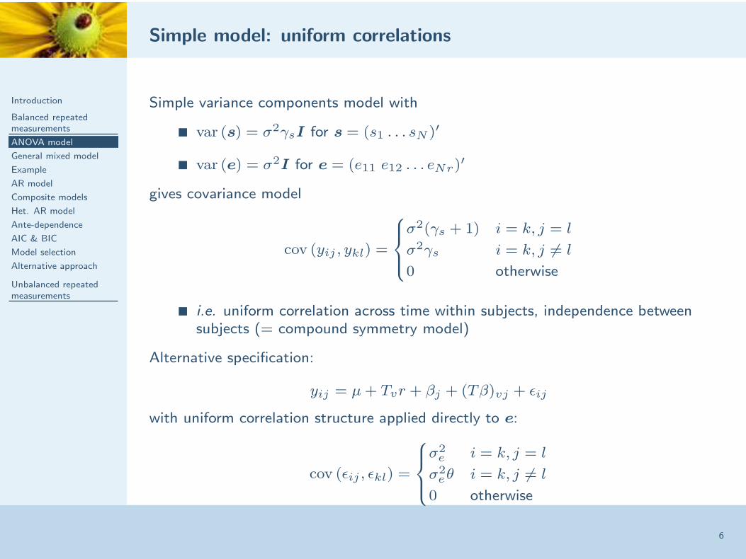
Simple variance components model with

■ var (s) = σ2γsI for s = (s1 . . . sN )′

■ var (e) = σ2I for e = (e11 e12 . . . eNr)′

gives covariance model

cov (yij , ykl) =

σ2(γs + 1) i = k, j = l

σ2γs i = k, j 6= l

0 otherwise

■ i.e. uniform correlation across time within subjects, independence betweensubjects (= compound symmetry model)

Alternative specification:

yij = µ+ Tvr + βj + (Tβ)vj + ǫij

with uniform correlation structure applied directly to e:

cov (ǫij , ǫkl) =

σ2e i = k, j = l

σ2eθ i = k, j 6= l

0 otherwise

Simple model: uniform correlations (2)

Introduction


ANOVA model

General mixed model

Example

AR model

Composite models

Het. AR model

Ante-dependence

AIC & BIC

Model selection



7

Equivalence between models:

σ2

e = σ2(γs + 1); θ =γs

γs + 1

In symbolic form, write these random models as

1. variance components form: subject + subject.time

2. covariance model form: subject.uniform(time)

In GenStat, model specification

1. vcomp [fixed=Tmt*Time] random=Subject/Time

2. vcomp [fixed=Tmt*Time] random=Subject.Time

vstructure [term=Subject.Time] factor=Subject,Time; \

model=identity,uniform

Matrix forms of model

Introduction


ANOVA model

General mixed model

Example

AR model

Composite models

Het. AR model

Ante-dependence

AIC & BIC

Model selection



8

Model 1:y =Xτ +Zu+ e

where

■ y = (y11 y12 . . . y1r y21 . . . yNr)′

■ τ = (µ T1 . . . Tg β1 . . . βr (Tβ)11 . . . (Tβ)gr)′ is the combined set of fixedeffects with (Nr × (r + 1)(g + 1)) design matrix X defining treatment (andtime) allocations to units

■ u= (s1 . . . sN )′ is the set of subject effects with (Nr ×N) design matrixZ = IN ⊗ 1r defining the allocation of units to subjects withvar (s) = σ2γsI

■ var (e) = σ2I for e = (e11 e12 . . . eNr)′

Hencevar (y) = σ2(γZZ′ + In) = σ2

{

γ(IN ⊗ 1r1′r) + In)

}

where n = Nr is the total number of observations.

Note in this form σ2s ≥ 0.

Matrix forms of model

Introduction


ANOVA model

General mixed model

Example

AR model

Composite models

Het. AR model

Ante-dependence

AIC & BIC

Model selection



9

Model 2:y =Xτ + ǫ

where

■ var (ǫ) = σ2e(IN ⊗C) for ǫ = (ǫ11 ǫ12 . . . ǫNr)′ and

■ C = [cij ] has cii = 1 for i = 1 . . . r, cij = θ for i 6= j, i, j = 1 . . . r

Hencevar (y) = var (ǫ) = σ2

e(IN ⊗C).

In this parameterization, the only constraint on the correlation parameter θ is|θ| < σ2.

Negative correlations are allowed - but may only be meaningful in certain specificcircumstances:

■ successive harvesting: a larger harvest in one period might result in lessproduce available in the next period

■ weight loss: a person losing a lot of weight in one period may be less vigilantin the next period

In both these cases, we might argue that the cumulative variable is more interestingthan period-wise increments (cf height vs growth per period).

General linear mixed model

Introduction


ANOVA model

General mixed model

Example

AR model

Composite models

Het. AR model

Ante-dependence

AIC & BIC

Model selection



10

We can generalise our definition of the linear mixed model to accommodate bothforms of the model:

y =Xτ +Zu+ e

As previously, the fixed and random effects may be partitioned into termsassociated with explanatory variables:

■ X = [X1 X2 . . .Xb ]

■ where Xi is an n× pi design matrix for the ith fixed term,∑

i pi = p

■ Z = [Z1 Z2 . . .Zc ]

■ where Zj is an n× qj design matrix for the jth random term,∑

j qj = q

■ τ ,u are partitioned conformally

◆ τ = (τ ′1. . .τb)

′

◆ u= (u′1. . .uc)′

◆ with ui ∼ N(0qi, σ2Gi) for some valid covariance matrix Gi and

cov(ui,uj) = 0

◆ e ∼ N(0n, σ2R) for some valid covariance matrix R, withcov(e,uj) = 0

General linear mixed model (2)

Introduction


ANOVA model

General mixed model

Example

AR model

Composite models

Het. AR model

Ante-dependence

AIC & BIC

Model selection



11

The variance matrix of the data takes the form

var(y) = σ2(ZGZ′ +R)

= σ2(c

∑

i=1

ZiGiZ′i +R)

= σ2H

for G= ⊕Gi.

In general, both G=G(ψ) and R = R(φ) may be functions of unknownparameters which are to be estimated via REML.

Results written in terms of a general value of H previously still hold in the modelgeneral model, but some further generalization is required.

For example, if we write κ = (ψ′,φ′)′, then the full set of variance parameterstakes the form (σ2,κ′)′.

General linear mixed model (3)

Introduction


ANOVA model

General mixed model

Example

AR model

Composite models

Het. AR model

Ante-dependence

AIC & BIC

Model selection



12

The log-likelihood function ℓ2 = ℓ(σ2,κ;y2) still takes the same form:

ℓ2 = −1

2

{

c(X) + (n− p) log(σ2) + log |H| + log |(X′H−1X)| + y′Py/σ2}

although now

H−1 = R−1 −R−1Z(Z′R−1Z +G−1)−1Z′R−1

The derivative of ℓ2 with respect to σ2 is unchanged, but derivatives with respectto elements of κ must also consider the form of

∂H

∂ψi

= Z∂G

∂ψi

Z′ ;∂H

∂φj

=∂R

∂φj

The form of τ is unchanged, with

u=GZ′Py = (Z′R−1Z +G−1)−1Z′R−1(y−Xτ)

and the mixed model equations are extended to take account of R as

[

X′R−1X X′R−1Z

Z′R−1X Z′R−1Z +G−1

] (

τ

u

)

=

(

X′R−1y

Z′R−1y

)

Finallye = y−Xτ −Zu= RPy

Example

Introduction


ANOVA model

General mixed model

Example

AR model

Composite models

Het. AR model

Ante-dependence

AIC & BIC

Model selection



13

■ Repeated measurements of rat weights

■ 27 rats allocated to 3 treatment groups: 10 control, 10 treated withchemical thiour, 7 treated with thyrox

■ Measurements taken weekly over 5 weeks

Estimated variance parameters

Introduction


ANOVA model

General mixed model

Example

AR model

Composite models

Het. AR model

Ante-dependence

AIC & BIC

Model selection



14

Model 1=======

Estimated variance components ( 75.54+51.47 = 127.0 )----------------------------- ( 75.54/127.0 = 0.5948 )Random term component s.e.rat 75.54 24.82Residual variance model-----------------------Term Factor Model(order) Parameter Estimate s.e.rat.week Identity Sigma2 51.47 7.43

Model 2=======

Residual variance model-----------------------Term Factor Model(order) Parameter Estimate s.e.rat.week Sigma2 127.0 25.5

rat Identity - - -week Uniform theta1 0.5948 0.0884


Introduction


ANOVA model

General mixed model

Example

AR model

Composite models

Het. AR model

Ante-dependence

AIC & BIC

Model selection



15

What happens if we put in both forms of uniform correlation?

vcomp [fixed=Tmt*Time] random=Subject/Timevstructure [term=Subject.Time] factor=Subject,Time; model=identity,uniform

Estimated variance components-----------------------------Random term component s.e.rat 63.50 aliasedResidual variance model-----------------------Term Factor Model(order) Parameter Estimate s.e.rat.week Sigma2 63.50 12.74


■ there are only two independent parameters in the model (dependence is notlinear)

■ no information left after two parameters have been fitted

■ aliased indicates that the parameter cannot be optimised (usually sticks atstarting position - here γs = 1 hence σ2

s = σ2)


Introduction


ANOVA model

General mixed model

Example

AR model

Composite models

Het. AR model

Ante-dependence

AIC & BIC

Model selection



16

vcomp [fixed=Tmt*Time] random=Subject/Timevstructure [term=Subject.Time] factor=Subject,Time; model=identity,uniform

Estimated variance components-----------------------------Random term component s.e.rat 63.50 aliasedResidual variance model-----------------------Term Factor Model(order) Parameter Estimate s.e.rat.week Sigma2 63.50 12.74


■ variance = σ2(γs + 1) = 2σ2 = 127.0

■ correlation = (γs + θ)/(γs + 1) = (1 + θ)/2 = 0.5948

■ so answer is correct but in a slightly unusual form

■ better to resolve cause of aliasing, than to untangle results

■ in general case, aliasing may cause algorithm to fail

Check residuals

Introduction


ANOVA model

General mixed model

Example

AR model

Composite models

Het. AR model

Ante-dependence

AIC & BIC

Model selection



17

Now we have a choice of residuals - from model 1 or model 2

■ in general, residuals from correlated structures may be pre-whitened, ie for

var(e) = σ2R

residuals are whitened asew = L−1e

where LL′ = R and e = RPy.

■ the ’best’ form of residuals for diagnostics in the linear mixed model is anunresolved issue, see eg Haslett & Dillane (1999)

■ in GenStat, residuals are not standardized, not whitened

■ then we expect residuals to reflect correlation pattern of fitted matrix

1. residuals expected to be independent

2. residuals should reflect uniform correlation structure (??)

■ in this case it makes sense to examine model 1 residuals, which should beindependent with equal variance

Residuals from model 1

Introduction


ANOVA model

General mixed model

Example

AR model

Composite models

Het. AR model

Ante-dependence

AIC & BIC

Model selection



18

■ residuals for each subject are joined by lines

■ for independent residuals we expect no pattern

■ here there is evidence of temporal correlation, as might be expected

■ more sophisticated correlation model required to capture variance pattern

Auto-regressive model

Introduction


ANOVA model

General mixed model

Example

AR model

Composite models

Het. AR model

Ante-dependence

AIC & BIC

Model selection



19

Most common model for temporal correlation for equally-spaced data isauto-regressive model of order 1 (AR1):

yij = µ+ Tv + βj + (Tβ)vj + eij

with AR1 correlation structure applied directly to e:

cov (eij , eil) = σ2φ|j−l|

This can be written symbolically as subject.AR1(time).

It is easily adapted to unequally-spaced data by using its continuous time analogue:

cov (eij , eil) = σ2φ|tj−tl|

where tj is the time at which measurement j was taken.

This is often called the exponential correlation function (the power model inGenStat).

Auto-regressive model

Introduction


ANOVA model

General mixed model

Example

AR model

Composite models

Het. AR model

Ante-dependence

AIC & BIC

Model selection



20

For equally spaced data, the covariance matrix across times within subjects thentakes the form:

C =

1 φ φ2 φ3 . . . φr−2 φr−1

φ 1 φ φ2 . . . φr−3 φr−2

φ2 φ 1 φ . . . φr−4 φr−3

. . .

φr−3 φr−4 φr−5 φr−6 . . . φ φ2

φr−2 φr−3 φr−4 φr−5 . . . 1 φφr−1 φr−2 φr−3 φr−4 . . . φ 1

with inverse

C−1 =1

1 − φ2

1 −φ 0 0 . . . 0 0−φ 1 + φ2 −φ 0 . . . 0 00 −φ 1 + φ2 −φ . . . 0 0

. . .

0 0 0 0 . . . −φ 00 0 0 0 . . . 1 + φ2 −φ0 0 0 0 . . . −φ 1

The inverse is sparse (tri-diagonal) and easier to work with.

Fitted AR1 model & residual plots

Introduction


ANOVA model

General mixed model

Example

AR model

Composite models

Het. AR model

Ante-dependence

AIC & BIC

Model selection



21

vcomp [fix=trt*week] rat.weekvstruc [rat.week] factor=week; model=ar

Residual variance model-----------------------

Term Factor Model(order) Parameter Estimate s.e.rat.week Sigma2 137.5 36.2

rat Identity - - -week AR(1) phi_1 0.8821 0.0362

High serial correlation + suggestion of variance increasing with time . . .

Composite models

Introduction


ANOVA model

General mixed model

Example

AR model

Composite models

Het. AR model

Ante-dependence

AIC & BIC

Model selection



22

Might consider a composite model:

yij = µ+ Tv + βj + (Tβ)vj + si + eij + aij

with AR1 correlation structure applied directly to e:

cov (eij , ekl) = σ2φ|j−l|

■ and s ∼ N(0, σ2sI) to add uniform correlation across time

■ this might arise from intrinsic subject differences which stay constant overtime

■ and a ∼ N(0, σ2sI) to add additional independent error

■ this might arise from measurement error on top of the correlated process

■ although plausible mechanisms for these extra terms exist, there is rarelysufficient data to fit them all successfully

■ variograms can be useful in indicating where extra terms required

Composite models

Introduction


ANOVA model

General mixed model

Example

AR model

Composite models

Het. AR model

Ante-dependence

AIC & BIC

Model selection



23

■ For this data, full composite model fails

■ Model with additional measurement error fails

■ Model with additional subject effects successfully fits the model, but AR1and subject term are clearly competing for correlation:

Estimated variance components-----------------------------Random term component s.e.rat -824.4 112.2

Residual variance model-----------------------Term Factor Model(order) Parameter Estimate s.e.rat.week Sigma2 909.8 123.8

rat Identity - - -week AR(1) phi_1 0.9771 0.0033

■ Unexpected estimates may be trying to tell you something about the model...

Composite models (2)

Introduction


ANOVA model

General mixed model

Example

AR model

Composite models

Het. AR model

Ante-dependence

AIC & BIC

Model selection



24

■ This is very much a variance modelling process

■ Appears to clash with model determination process discussed earlier?

■ May be a problem retaining terms from randomization process with somevariance models, e.g. subject+subject.ar(week)

■ However, this often occurs because terms compete for similar elements ofcovariation

■ Pragmatic approach best - retain randomization terms if no other term isequivalent (or close) or if can sensibly fitted within good variance model

Heterogeneous AR model

Introduction


ANOVA model

General mixed model

Example

AR model

Composite models

Het. AR model

Ante-dependence

AIC & BIC

Model selection



25

We can account for variance heterogeneity apparent in residual plots eitherindirectly via transformation, or directly by modelling the heterogeneity.

Heterogeneous AR1 correlation structure applied directly to e:

cov (eij , eil) = σjσlφ|j−l|

In matrix termsvar (e) = IN ⊗ (D0.5CD0.5 )

where

■ D is a r × r diagonal matrix with entries σ2

i , i = 1 . . . r

■ C is a r × r correlation matrix of form AR1

■ pre- and post-multiplication means this is termed outside heterogeneity inGenStat

Ante-dependence model

Introduction


ANOVA model

General mixed model

Example

AR model

Composite models

Het. AR model

Ante-dependence

AIC & BIC

Model selection



26

■ An alternative generalization of the AR model is the antedependence model(AD).

■ The AR1 model for e can be construed as

et = φet−1 + at for t large

■ where a ∼ N(0,D), for D = I

■ |φ| < 1

Note that t is taken to be large so that system is in a steady state.

It follows thatU′e = a

where U is an upper triangular matrix with value 1 on the diagonal, −φ on the firstoff-diagonal and zero elsewhere.

Ante-dependence model

Introduction


ANOVA model

General mixed model

Example

AR model

Composite models

Het. AR model

Ante-dependence

AIC & BIC

Model selection



27

It follows that

U′var (e)U = var (a)

var (e) = (U′)−1DU−1

var (e) = (UDU′)−1

Generalization of the AR1 model to

et = φtet−1 + at for t > 1

where a ∼ N(0,D), for D = diag{di; di > 0}

This is the ante-dependence model of order 1

■ with covariance matrix C = (UDU′)−1

■ where off-diagonal elements of U are now {−φt}

■ Generalization to higher orders follows by adding lags of et−2 etc

Comparison of variance models

Introduction


ANOVA model

General mixed model

Example

AR model

Composite models

Het. AR model

Ante-dependence

AIC & BIC

Model selection



28

■ Likelihood ratio tests are valid only for nested models

■ Can use information criteria to compare non-nested variance models (withsame fixed effects)

■ For a mixed model fitted by REML with

◆ Nv variance parameters estimated

◆ n data values

◆ p DF fitted for fixed terms

◆ log-likelihood function maximised under model as RL

■ AIC = −2RL+ 2Nv (Akaike Information Criterion)

■ BIC/SBC = −2RL+Nv log(n− p) (Bayesian/Schwarz IC)

■ BIC tends to be more conservative than AIC

■ for criterion chosen, variance model with lowest IC value is chosen

Model selection via IC

Introduction


ANOVA model

General mixed model

Example

AR model

Composite models

Het. AR model

Ante-dependence

AIC & BIC

Model selection



29

For rats data

■ n = 135

■ for fixed=trt*week, p = 15

■ n− p = 120

Model -2RL Nv AIC BICUniform 676.57 2 680.52 686.14AR(1) 599.09 2 604.09 608.66Het. AR(1) 548.61 6 560.61 577.33AD(1) 544.56 9 562.56 587.65AD(2) 519.58 12 543.58 577.02US 517.55 15 547.55 589.36

■ In this case, agreement between criteria

■ Ordering different: BIC favours more parsimonious models

Impact on fixed effect SEDs

Introduction


ANOVA model

General mixed model

Example

AR model

Composite models

Het. AR model

Ante-dependence

AIC & BIC

Model selection



30

Several purposes of modelling covariance structure:

■ to understand patterns of variance and correlation

■ to get more appropriate SEDs for fixed effects and PEVs for random effects

Compare SEDs from two models for rat data:

Uniform correlation model Unstructured variance model

week 1 * *week 2 1.98 * 0.96 *week 3 1.98 1.98 * 1.42 0.98 *week 4 1.98 1.98 1.98 * 2.35 2.15 1.29 *week 5 1.98 1.98 1.98 1.98 * 3.03 2.92 2.11 1.16 *

week 1 week 2 week 3 week 4 week 5 week 1 week 2 week 3 week 4 week 5

■ Unstructured model reflects both changing variance and correlation


Introduction


ANOVA model

General mixed model

Example

AR model

Composite models

Het. AR model

Ante-dependence

AIC & BIC

Model selection



31

This analysis fits treatment means at each time-point and uses the covariancematrix to describe the nature of individual variation about treatment means.

There is clear linear trend over time in the profiles and the current analysis does notexploit this structure. We might therefore try an alternative model:

yij = µ+ Tv + atj + bvtj + eij

with a suitable correlation structure applied directly to e:

var (e) = σ2IN ⊗C

This model fits linear trend in t, with a separate intercept (µ+ Tv) and slope(a+ bv) for each treatment group.

However, if the linear trend is a poor fit to the mean profiles, then the covariancestructure will describe the lack of fit as well as variation about treatment means.

If we use the modified model

yij = µ+ Tv + atj + βj + bvtj + (Tβ)vj + eij

then the additional term βj fits the overall mean at each time exactly, and (Tβ)vj

fits the treatment mean at each time point exactly.

Alternative approach (2)

Introduction


ANOVA model

General mixed model

Example

AR model

Composite models

Het. AR model

Ante-dependence

AIC & BIC

Model selection



32

If the model terms are fitted in the order given, then these terms can be used totest for lack of fit of the linear trend model.

In symbolic terms, this model could be represented as

■ fixed = Trt + t + fac(t) + Trt.t + Trt.fac(t)

■ random = Subject.Cov(Time)

where t represents the numeric variate, and Trt represents the treatment factor.

Tests for rat data:

Sequentially adding terms to fixed model

Fixed term Wald statistic n.d.f. F statistic d.d.f. F prtrt 4.09 2 2.05 24.2 0.151time 1407.18 1 1407.18 25.5 <0.001cweek 35.71 3 11.11 25.8 <0.001trt.time 24.77 2 12.38 25.5 <0.001trt.cweek 27.84 6 4.26 32.3 0.003

where cweek is a copy of the week factor = fac(t), time=t, trt=Trt.

Alternative approach (3)

Introduction


ANOVA model

General mixed model

Example

AR model

Composite models

Het. AR model

Ante-dependence

AIC & BIC

Model selection



33

Adding a quadratic term (timesqrd) removes the group-specific lack of fit -although still some lack of fit to overall means at each time:

Sequentially adding terms to fixed model

Fixed term Wald statistic n.d.f. F statistic d.d.f. F prtrt 4.09 2 2.05 24.2 0.151time 1407.18 1 1407.18 25.2 <0.001timesqrd 0.09 1 0.09 25.9 0.769cweek 35.63 2 17.22 26.2 <0.001trt.time 24.77 2 12.38 25.2 <0.001trt.timesqrd 20.02 2 10.01 25.9 <0.001trt.cweek 7.82 4 1.87 30.0 0.141

Removing the lack of fit terms has some impact on the across time covariancemodel (AD2):

Covariance matrix with lack of fit terms Covariance model omitting lack of fit1 21.6 1 22.62 33.0 68.7 2 35.6 75.73 31.6 69.1 94.8 3 33.4 74.0 99.24 27.8 64.5 116.4 181.6 4 33.4 77.0 128.9 218.55 24.9 60.1 122.9 207.2 268.4 5 32.3 75.4 134.9 242.4 302.0

1 2 3 4 5 1 2 3 4 5

Unbalanced data

Introduction



Unbalanced data

Technical note

RCR model

RCR variance model

Example

RCR variance model

RCR and direct products

Computational issues

Exercise

References

34

In many cases, longitudinal data will not be balanced in either the allocation oftreatments to subjects or in terms of number and frequency of measurements.

Each subject (i = 1 . . . N) then has their own vector of ni measurement timesti = (ti1 . . . tini

) and the model is usually written in general terms as

yij = µ+ f(tij) + fv(tij) + eij

where f() is a function describing the population mean profile and fj() describesdeviations of treatment group v from the mean profile.

If subjects are measured at different times, then fitting treatment means at eachtime results in an over-parameterized model that gives little insight into the process.

The variance model for the data (ordered by subjects) is usually written as

var (e) = ⊕{Ci}; i = 1 . . . N

where Ci is the across-time covariance matrix for subject i, and the overall variancematrix is block diagonal.

These covariance matrices will be determined by the same underlying model (egAR1) but will take different numeric values due to the differing sets of measurementtimes.


Introduction



Unbalanced data

Technical note

RCR model

RCR variance model

Example

RCR variance model



Exercise

References

35

The direct product structure is convenient as has a simple inverse

(IN ⊗C)−1 = IN ⊗C−1

whereas the direct sum structure has inverse

⊕{C−1

i }

In the former case, C has to be inverted once but in the latter each Ci may haveto be inverted separately, and matrix multiplications involving R−1 arecorrespondingly more complex.

If the imbalance is slight eg. an overall set of common measurement times with afew missing values, then it may be computationally more efficient to include themissing measurements to retrieve the balanced structure.

Consider the model

yij = µ+ f(tj) + fv(tj) + eij for tjpresent for subjecti

0 = θij + µ+ f(tj) + fv(tj) + eij for tjabsent for subject i


Introduction



Unbalanced data

Technical note

RCR model

RCR variance model

Example

RCR variance model



Exercise

References

36

Consider the model

yij = µ+ f(tj) + fv(tj) + eij for tjpresent for subjecti

0 = θij + µ+ f(tj) + fv(tj) + eij for tjabsent for subject i

The parameters θij are known as ’missing value covariates’ with θij = −yij attimes j with no data on subject i and all other estimates are unchanged (see eg.Gilmour et al, 2004).

On rearranging these equations back into time order for each subject, the directproduct structure of the variance model is retrieved.

Whether this is an efficient strategy depends on the number of missing values.

GenStat technical notes

Introduction



Unbalanced data

Technical note

RCR model

RCR variance model

Example

RCR variance model



Exercise

References

37

GenStat deals poorly with direct sum structures - its efficient algorithm is builtupon direct product structures. Together with its automatic determination of theresidual term, this assumption can lead to surprising results.

Consider a balanced repeated measures structure with several missing values andcorrelation across time within subject IN ⊗C.

■ Then the size of covariance matrix IN ⊗C 6= the number of data valuespresent, so this term cannot be used as residual matrix R

■ But, a model must have a residual term

■ So an identity residual term is added (and specified in model summary)

■ Two ways to deal with this

◆ If lack of balance due to missing combinations: put thesecombinations into data set and use option [mvinclude=yvar] - good forfew missing values

◆ Explicitly specify extra residual term and fix component to value smallenough to not affect rest of model, but not so small it destabilizesfitting process - better for many missing combinations

Random coefficient regression

Introduction



Unbalanced data

Technical note

RCR model

RCR variance model

Example

RCR variance model



Exercise

References

38

Random coefficient regression (RCR) uses an individual model for each subject:

■ Population mean regression model with subject variation allowed inregression coefficients

■ Simplest version uses linear regression, may use higher order polynomials orother functions

■ Does not require any form of balance in data

■ Simple linear RCR model

yij = µ+ Tr + atij + brtij + ui + vitij + eij

◆ yij is jth measurement on subject i at time tij

◆ r = r(i) is the treatment combination allocated to subject i

◆ µ+ Tr fixed intercept for treatment r

◆ a+ br fixed slope for treatment r

◆ ui, vi random deviation in intercept, slope for subject i

◆ eij residual = random variation about subject i linear trend

Random coefficient regression (2)

Introduction



Unbalanced data

Technical note

RCR model

RCR variance model

Example

RCR variance model



Exercise

References

39

Matrix version of model for subject i:

yi = [1 ti]

[

µ+ Tr

a+ br

]

+ [1 ti]

[

ui

vi

]

+ ei

where yi is set of measurements for subject i taken at times ti = (ti1 . . . tini)′.

Note: design matrix for fixed and random effects are identical at subject level (iftreatment groups/covariates do not change over time).

To finish model, need to specify variance structure:

var

[

ui

vi

]

= C =

(

σ11 σ12

σ12 σ22

)

; cov

([

ui

vi

]

,

[

uj

vj

])

= 0

var

[

u

v

]

= C ⊗ IN

var (ei) = σ2I

Thenvar (yij) = σ11 + 2tijσ12 + t2ijσ22 + σ2.

RCR variance model

Introduction



Unbalanced data

Technical note

RCR model

RCR variance model

Example

RCR variance model



Exercise

References

40

The covariance σ12 is an essential part of the model, required to make it invariantto translations in t.

For example consider the model with the time covariate centered about its mean tµ:

yij = µ+ Tr + a(tij − tµ) + br(tij − tµ) + ui + vi(tij − tµ) + eij

= µ∗ + T ∗r + atij + brtij + ui + vi(tij − tµ) + eij

where µ∗ = µ− atµ, T ∗r = Tr − btµ.

If the variance matrix of the random effects is written as

var

[

ui

vi

]

= C =

(

σ∗11

σ∗12

σ∗12

σ∗22

)

then

var (yij) = σ∗11 + 2(tij − tµ)σ∗

12 + (tij − tµ)2σ∗22 + σ2

= σ∗11 − 2tµσ

∗12 + t2µσ

∗22 + 2(σ∗

12 − σ∗22tµ)tij + t2ijσ

∗22 + σ2

RCR variance model (2)

Introduction



Unbalanced data

Technical note

RCR model

RCR variance model

Example

RCR variance model



Exercise

References

41

var (yij) = σ∗11 + 2(tij − tµ)σ∗

12 + (tij − tµ)2σ∗22 + σ2

= σ∗11 − 2tµσ

∗12 + t2µσ

∗22 + 2(σ∗

12 − σ∗22tµ)tij + t2ijσ

∗22 + σ2

This is equivalent to the original model if

σ11 = σ∗11 − 2tµσ

∗12 + t2µσ

∗22

σ12 = σ∗12 − σ∗

22tµ

σ22 = σ∗22

So a translation in t changes the form of the variance matrix - covariance parameterσ12 is required to keep the same model.

Example

Introduction



Unbalanced data

Technical note

RCR model

RCR variance model

Example

RCR variance model



Exercise

References

42

■ For rat data: little variation in intercept at t = 1, much variation at mean(t)

■ Clear positive association between intercept and slope at mean(t), much lessat t = 1

Example (2)

Introduction



Unbalanced data

Technical note

RCR model

RCR variance model

Example

RCR variance model



Exercise

References

43

For rat data, fitted RCR with time covariate centered or not:

Estimated parameters for covariance models------------------------------------------

Centered covariate: intercept at t=3 (correlation=0.78)

Random term(s) Factor Model(order) Parameter Estimate s.e.rat + rat.time Across terms Unstructured v_11 4.352 1.496

v_21 1.470 0.561v_22 0.8018 0.2964

Within terms Identity - - -

No centering: intercept at t=0 (correlation=-0.11)

Random term(s) Factor Model(order) Parameter Estimate s.e.rat + rat.time Across terms Unstructured v_11 1.678 0.749

v_21 -0.1331 0.3049v_22 0.8018 0.2964

Within terms Identity - - -

■ big change in intercept variance and covariances

■ with covariance, can transform between different scales t− c

■ without covariance, model may be inadequate & interpretation may be wrong

Implicit variance model

Introduction



Unbalanced data

Technical note

RCR model

RCR variance model

Example

RCR variance model



Exercise

References

44

RCR has implicit variance model

var (yi) =XiCX′i + σ2I

where Xi = [1 ti], or

var (yij) = σ11 + 2tjσ12 + t2jσ22 + σ2

■ this is a parsimonious quadratic variance function in terms of t

■ presence of covariance makes variance model more flexible

■ but - it may not match variance pattern of data - validation of modelimportant

■ sometimes more appropriate to fit fixed polynomial regression plus generalcovariance model

Rat data

■ quadratic + AD(2): -2RL=567.99, AIC=591.99, BIC=625.44

■ quadratic RCR: -2RL=587.34, AIC=601.34, BIC=620.85


Introduction



Unbalanced data

Technical note

RCR model

RCR variance model

Example

RCR variance model



Exercise

References

45

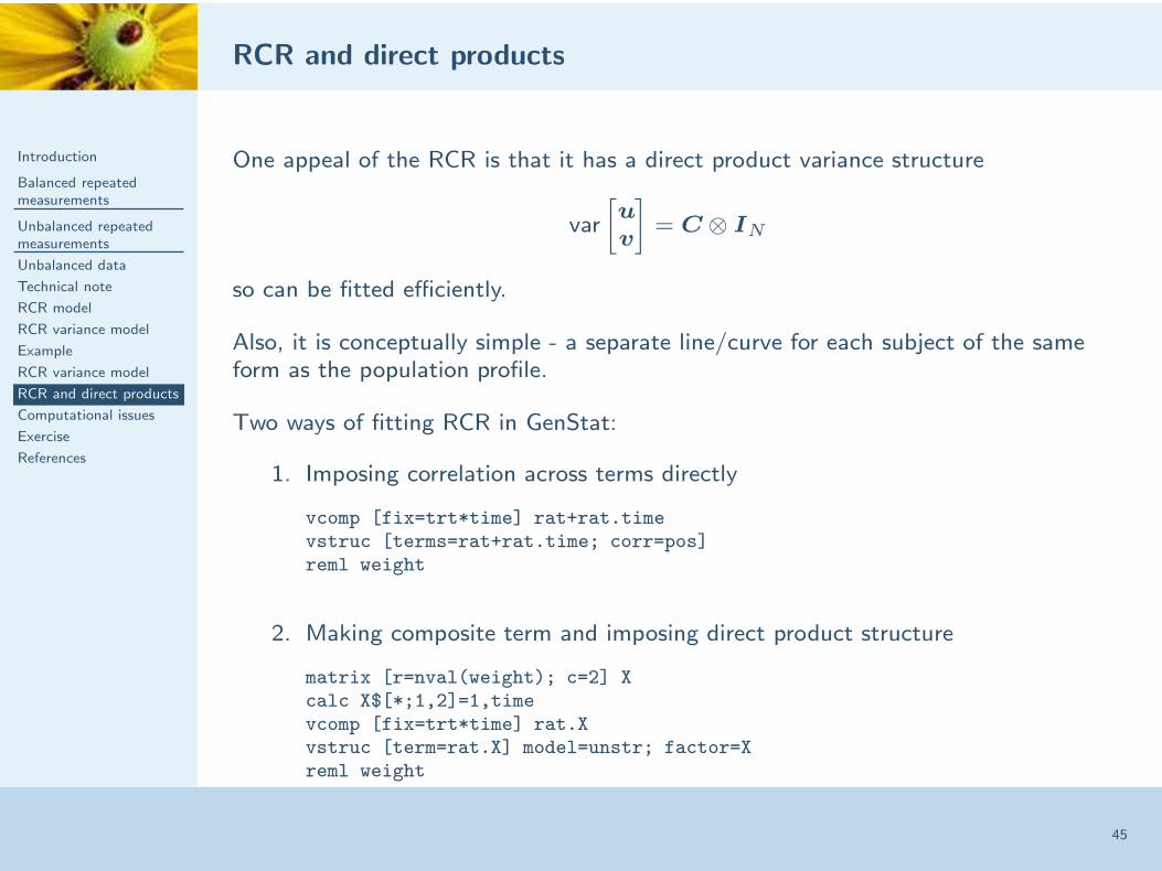
One appeal of the RCR is that it has a direct product variance structure

var

[

u

v

]

= C ⊗ IN

so can be fitted efficiently.

Also, it is conceptually simple - a separate line/curve for each subject of the sameform as the population profile.

Two ways of fitting RCR in GenStat:

1. Imposing correlation across terms directly

vcomp [fix=trt*time] rat+rat.timevstruc [terms=rat+rat.time; corr=pos]reml weight

2. Making composite term and imposing direct product structure

matrix [r=nval(weight); c=2] Xcalc X$[*;1,2]=1,timevcomp [fix=trt*time] rat.Xvstruc [term=rat.X] model=unstr; factor=Xreml weight


Introduction



Unbalanced data

Technical note

RCR model

RCR variance model

Example

RCR variance model



Exercise

References

46

Covariance parameters (σ12) in RCR can be difficult to estimate:

■ especially where the number of subjects is small (<20)

■ estimation tends to be more stable with centered covariates

■ one strategy to get initial values

◆ estimate subject intercept & slope parameters assuming no correlation

◆ estimate correlation between intercepts & slopes directly, ie corr(u,v)

◆ use these estimates as starting values

◆ works well for centered covariates

Exercise

Introduction



Unbalanced data

Technical note

RCR model

RCR variance model

Example

RCR variance model



Exercise

References

47

Grizzle & Allen dog data

■ Coronary sinus potassium concentrations measured on 36 dogs, dividedbetween 4 different treatment groups

■ Seven measurements were made on each dog, every 2 minutes from 1 to 13minutes after an event (occlusion)

■ Aim of this analysis is to quantify the difference in profiles betweentreatments: a good model is therefore required for both treatment meansand within-subject variation

■ Data are in spreadsheet dog.xls

■ Investigate different analyses for this data & decide on the most appropriateapproach

References

Introduction



Unbalanced data

Technical note

RCR model

RCR variance model

Example

RCR variance model



Exercise

References

48

Brien CJ & Bailey RA (2006) Multiple randomizations. Journal of the Royal Statistical Society, Series B,68, 571-599.

Fitzmaurice G, Davidian, M, Molenberghs G, & Verbeke G. (2008) Longitudinal Data Analysis

Chapman & Hall, CRC Press.Gilmour A, Cullis B, Welham SJ, Gogel BJ, Thompson R (2004) An efficient computing strategy for

prediction in mixed linear models. Computational Statistics and Data Analysis, 44, 571-586.Haslett, J. & Dillane, D. (2004) Application of ‘delete=replace’ to deletion diagnostics for variance

component estimation in the linear mixed model. Journal of the Royal Statistical Society, Series B 66,131–143.

Verbeke G & Molenberghs G (2000) Linear Mixed Models for Longitudinal Data, Springer, New York.

reml estimation and linear mixed models 3. analysis of

Documents