Munich Personal RePEc Archive

Remittances, trade liberalisation, and

poverty in Pakistan: The role of excluded

variables in poverty change analysis

Siddiqui, Rizwana and Kemal, A.R.

Pakistan Institute of Development Economics

October 2002

Online at https://mpra.ub.uni-muenchen.de/4228/

MPRA Paper No. 4228, posted 24 Jul 2007 UTC

Remittances, Trade Liberalisation, and Poverty in

Pakistan: The Role of Excluded Variables

in Poverty Change Analysis

RIZWANA SIDDIQUI and A. R. KEMAL*

This paper explores the impact of two shocks, trade liberalisation policies and decline in

remittances, on welfare and poverty in Pakistan. It begins by reviewing the economy, which

reveals that during the Nineties although import tariffs were reduced by 55 percent, poverty

however remained higher in this period than in the Eighties. At the same time, Pakistan has

experienced a slow down in the inflow of remittances, which reduces the incomes of

households and puts pressure on the exchange rate resulting in reduction in the inflow of

imports despite a reduction in import duties. Thus, in the absence of the effects of decline in

remittances, the analysis of the impact of trade liberalisation policies may render biased results.

This study overcomes this constriction and analyses the impact of trade liberalisation policies

in the absence and presence of decline in remittances in a CGE framework with all the features

necessary for trade policy analysis with poverty and remittances linkages. The simulation

results show that a decline in remittances reduces the gains from trade liberalisation. The

negative impact of remittance decline dominates the positive impact of trade liberalisation in

urban areas. But, the positive impact of trade liberalisation dominates the negative impact of a

decline in remittances in the case of rural areas. Poverty rises in Pakistan as a whole. It shows

that the decline in remittance inflows is a major contributory factor in explaining the increase

in poverty in Pakistan during the Nineties.

JEL classification: O53, O24, C68, I32

Keywords: Pakistan, Remittances, Trade Policy, CGE, Poverty

I. INTRODUCTION

With a view to protect its nascent industries against imports, Pakistan has pursued

protectionist trade policies since the 1950s. The industries enjoyed quite high levels of

protection in the 1950s, 1960s, and 1970s. The import regime comprised of both tariff

and non-tariff barriers. The latter included outright bans, quota restrictions, and imports

allowed to specific users through an elaborate licensing system. These policies led to

wasteful use of resources by encouraging import substitution even in those industries

Rizwana Siddiqui <rizwana_s99@yahoo.com> <rizwana_s99@hotmail.com> is a Research Economist

and Dr A. R. Kemal was Director of the Pakistan Institute of Development Economics, Islamabad at the time of

writing this paper.

Authors’ Note: We are thankful to anonymous referees of this journal for their helpful comments on an

earlier version of this paper. This paper is a part of the project entitled “Linkages of Globalisation and Poverty in

South Asian Countries. CGE based analysis” DFID-project, University of Warwick, UK”. We are also thankful to

Prof. John Whalley, University of Warwick, Prof. Jeff Round, University of Warwick, UK, Dr Howard White,

Senior Evaluation Officer, World Bank, Washington, D. C. USA and Dr Rehana Siddiqui, Chief of Research,

PIDE, Islamabad for their comments on the earlier version of this paper.

Siddiqui and Kemal

384

where the country did not have long-run comparative advantage. Consequently, the

distortion in resource allocation adversely affected the country’s economic and social

conditions. Inefficiency in resource use has been one of the factors in the slow growth of

output that has led to high levels of poverty in Pakistan.12 This calls for changes in

policies and incentives and the market mechanism that help to reduce poverty.

Pakistan adopted trade liberalisation policies in 1981 by reducing quantitative

restrictions and rationalising the tariff structure, which reduces the rate of protection.

Removal of import restrictions has a two-fold impact on poverty.23 The first effect is that

a move towards free trade would increase the returns to the factor of production, which is

abundant in the country. In the case of Pakistan, labour is the abundant factor. Second,

the reduction in import duties, especially on raw materials and machinery, is expected to

result in a reduced cost of production and a reduction in prices. Similarly, reduction in

import duties on consumer goods implies the reduction in the prices of imported finished

products and import substitution activities. This helps in increasing real incomes. Tariff

reduction, therefore, is expected to help in an improvement in aggregate welfare and a

reduction in poverty.

The empirical evidence on poverty and income inequality in Pakistan, however,

contradicts the optimism of the proponents of trade liberalisation. Because Pakistan has

experienced a rise in poverty and income inequality during the period of trade

liberalisation. However, such an outcome may be defensible in view of the fact that along

with the liberalisation in imports, Pakistan has also experienced a slow down in the

inflow of remittances. The reduction in remittance inflow reduces the incomes of

households and puts pressure on the exchange rate resulting in a reduction in the inflow

of imports despite a reduction in import duties. Therefore, without incorporating

remittances in the analysis to explore the impact of trade liberalisation on poverty, the

results may be biased. In this study, we include the decline in remittances in presence of

trade liberalisation for poverty change analysis. Poverty is expected to decline if the

impact of trade liberalisation dominates the impact of decline in remittances, but would

tend to rise if the impact of the reduction in remittances dominates.

The present study proposes to assess the impact of two phenomenon on poverty by

exploring the question: whether trade liberalisation or decline in remittances or both are

responsible for the increase in poverty and inequality in Pakistan? The examination is done

through the computable general equilibrium (CGE) framework. The model used in this study

is closely related to previous CGE models built in various studies [see Decaluwe, et al.

(1999)]. This paper presents a similar model that is developed for trade policy analysis in

Pakistan under the Micro Impact of Macro Adjustment Policies (MIMAP) project by Siddiqui

and Iqbal (1999b) and extended in the latter studies for MIMAP [see Siddiqui, et al. (1999a)

and Kemal, et al. (2001); Siddiqui and Kemal (2006)].

The plan of the study is as follows. The next section reviews the economy of

Pakistan with particular reference to trade policies, structure of trade, remittance inflow

and poverty levels. Section III summarises the results of the studies focusing on trade

1One-third of the population still lives below the poverty line. 2The Stolper-Samuelson theorem suggests that the per capita income differentials due to existing factor

endowment differentials tend to disappear over time after trade liberalisation [for details see Krugman and

Obstfeld (1994)].

Remittances, Trade Liberalisation, and Poverty

385

liberalisation, remittances and poverty linkages. Section IV presents data for the base

year, discusses the methodology and model briefly. The results of the analysis are

presented in Section V and Section VI concludes the paper.

II. REVIEW OF ECONOMY

(a) Trade Policies

Pakistan has maintained a complex system of trade policy regime since 1952.

Import bans, quota, licensing requirements, other restrictions34 imposed to protect the

domestic industry, and high tariffs have introduced serious distortions. The high tariffs

imposed for protecting domestic industries and to raise revenues, have become counter-

productive. They have resulted in smuggling and corruption. Neither the revenue nor the

protection objectives were achieved. Besides, until the mid-1980s, the non-tariff

restrictions have remained binding, as the prices of imported goods, in general, have been

higher than the landed cost. In 1981, about 41 percent of industrial value added was

protected by import bans and another 22 percent by various forms of import restrictions

[Kemal, et al. (1994)].

Pakistan has initiated reforms in the trade regime in the early 1980s, with a

view to creating an efficient and competitive manufacturing industry through an easy

access to raw material, intermediate goods and machinery. The trade policy has been

gradually liberalised and the producers have been exposed to the global market as it

strives to make the local industry efficient and competitive. In the 1980s quota

restrictions were removed. In the 1990s the Restricted List was eliminated and those

items that were to be restricted due to Health and Safety Requirements and

Procedural Requirements have been added to the Negative List. For protecting the

industries, tariffs are being used instead of quantitative restrictions (QRs). During

1983-84 to 1993-94, 724 items were removed from the Negative List. Over all, the

number of intermediate goods, consumer goods and capital goods on the negative list

were reduced from 142 to 16, 32 to 7 and 221 to 107, respectively. At present, the

negative list comprises only of 62 products mostly on religious, environmental,

security and health grounds. Import licensing has gradually declined since 1981. And

by the year 1993, it was eliminated. Now only an insignificant portion of total

imports is subject to quantitative restrictions (QRs).45 All these changes resulted in a

decline in protection rates.

Table 1 presents the implicit nominal protection rate (NPRI) that takes into

consideration the tariff equivalent of quota and the explicit nominal protection rate

(NPRE). It shows that the percentage of industries where NPRI>NPRE fell from 34.4

percent to 2 percent of manufacturing industries over the 1981-91 period. This indicates

that quota restrictions were almost non-existent in the later period. Table 1 also shows

Table 1

3Import of capital goods was restricted through licensing, value limit and specificity of importers

[World Bank (1989)]. 4The banned items, on the “Negative List”, also include some textile products such as woven cotton

fabrics, woven synthetic fabrics, bed linens, curtains, certain knitted fabrics and apparel items, tents, carpets and

textiles floor coverings. However, all of these have been removed in 2001.

Siddiqui and Kemal

386

Industries Protected by Tariff and Non-tariff Barriers

Percentage of Industries

Nominal Protection 1980-81 1990-91

NPRI > NPRE 34.4 2.0

NPRI < NPRE 57.8 71.7

NPRI = NPRE 7.8 26.3

Source: Kemal, et al. (1994).

that NPRI fell short of NPRE, i.e., tariffs were prohibitively high, for 71.7 percent of the

industries in 1990-91 compared with 57.8 percent in 1980-81 and the percentage of

industries where tariffs were the binding constraints have increased from 7.8 percent to

26.3 percent industries over 1981-91. In the presence of non-tariff barriers, tariffs play a

minor role. However, with the removal of non-tariff barriers the protection levels

becomes transparent. During the adjustment period tariffs have played a larger role in

providing protection to industries.

After reducing QRs, Government of Pakistan (GOP) focused on a rationalisation of the

tariff structure; reducing tariff rates and their dispersion. During 1988-91, tariffs were reduced

on 1134 items and increased on 462 items. The maximum tariff rate was reduced from 225

percent to 100 percent. It was further reduced to 65 percent in June 1995. The number of tariff

slabs was reduced from 17 to 10 during the same time period. Recently, the maximum tariff

rate was reduced to 25 percent except for automobiles and alcoholic drinks and the number of

tariff slabs has been reduced to four [Pakistan (Various Issues a, b)].

Tariff rationalisation during the Nineties resulted in a decline in tariff rates on all

categories of imports. On final capital goods, the tariff rate declined from 19.5 percent to

7.3 percent, on final consumer goods from 24.6 percent to 9.6 percent, on raw material

for capital goods from 31.9 percent to 15.4 percent and on raw material for the consumer

goods from 19.5 to 10.6 percent. The average tariff rate was reduced by 55 percent, from

22.2 percent in 1987-88 to 9.7 percent in 1999-2000 (Table 2). Recently, these tariff rates

further reduced by 3, 6, 10 and 7 percentage points, respectively. On average, tariff rate

declined by 4 percentage points during the period 2000-04.

Table 2

Tariff Structure by Commodity Group (Percentages)

Final Imports of Raw Material

Years Capital

Goods

Consumer

Goods

Capital

Goods

Consumer

Goods

Average

Tariff Rate

1980-81 32.15 28.42 34.06 13.79 22.06

1984-85 15.02 17.66 94.09 12.94 19.19

1987-88 19.54 24.56 31.92 19.53 22.22

1988-89 18.55 14.32 24.38 18.38 17.37

1989-90 19.77 11.53 23.32 20.12 17.48

1994-95 12.48 13.90 31.56 20.85 17.84

1999-00 7.29 9.55 15.36 10.60 9.86

2003-04 3.83 3.53 5.10 3.53 6.03

Source: Data on imports and tariff revenue are taken from Economic Survey [Pakistan (Various Issues b)] and

CBR Year Book [Pakistan (Various Issues a)], respectively.

(b) Structure of Trade

Remittances, Trade Liberalisation, and Poverty

387

Like most of the developing countries, Pakistan is dependent on agricultural-based

exports. For a diversification of exports, it has to rely on imported raw materials,

machinery, and capital goods for industrialisation. A comparison of the structure of trade

during the Eighties and Nineties shows that the composition of imports by economic

classification has not changed much over twenty years in spite of trade liberalisation. The

share of imported capital goods in total imports has increased from 28 percent in 1980-81

to 37 percent in 1985-86, but due to a slow down in the economy, especially in the

industrial sector, import of capital goods declined to 25 percent by 2000-01. Recent

increases in growth boosted investment which resulted in a sharp increase in imports of

capital goods to 36 percent in 2004-05. The share of raw materials for consumer goods

also shows a declining trend over the whole period, it declined from 50 percent in 1980-

81 to 40 percent in 1985-86, but since then it has increased to around 46 percent by 2004-

05. On the other hand, the share of imported inputs for capital goods has remained less

than 10 percent throughout the period. The share of imports of final consumer goods

increased from 14 percent to 18 percent over the 1980-86 time period and in the next 20

years its share declined to 10 percent (Table 3).

The structure of exports shows significant changes over time. The share of exports

of primary goods, in 2005, is one-fourth of the 1980-81 level. The share of exports of

semi-manufactured goods has increased from 11 percent to 24 percent over the 1980-81

to 1990-91 period, but declined to 10 percent in the subsequent period. The exports of

manufactured goods, however, show a consistently rising trend; its share increases from

45 percent to 79 percent over the twenty-five year period (Table 3).

Reductions in quantitative restrictions (QRs), reductions in tariff rates,

increase in imports, increase in exports, the sum of exports and imports as a

percentage of GDP are the usual indicators used to measure the degree of openness.

QRs were almost non-existent in the 1990s. On average, the tariff rate declined by 73

percent during 1981-2005. It is important to note that in spite of the reduction in

trade restrictions, imports as a percentage of GDP show a declining trend over the

twenty-five year period: imports declined from 22.3 percent of GDP in 1980-81 to

20.5 percent of GDP in 200556 (Table 4). However, exports as a percentage of GDP

show an increasing trend, from 12.8 percent of GDP in 1980-81 to 16.4 percent of

GDP in 2004-05. The most commonly used indicator for openness is the total of

exports and imports as a ratio of GDP, this indicator shows that despite a decline in

imports, openness shows a slight increase, from 35.2 percent to 36.9 percent over

twenty-five years (Table 4). The reduction in both tariffs and non-tariff barriers may

seem surprising, but it needs to be underscored that during the 1990s because of

inadequate foreign exchange reserves, the government had to resort to frequent

devaluation making the imports expensive. Furthermore, low-level of economic

activity constrained the demand for surplus goods.

5The following factors are responsible for this decline. First, remittances declined very significantly,

from $2.9 billion in 1982-83 to $1 billion in 1999. They were used to finance the trade deficit for a long time.

Second, steep devaluation resulted in a lower level of imports. Third, economic activity slowed down in the

1990s.

Siddiqui and Kemal

388

Table 3

Structure of Trade by Economic Classification (Percentages)

Imports of Exports

Raw Material for

Years

Capital

Goods Capital

Goods

Consumer

Goods

Consumer

Goods

Total Primary Semi-

manufactured

Manufactured Total

1980-81 28 8 50 14 100 44 11 45 100

1985-86 37 5 40 18 100 35 16 49 100

1990-91 33 7 44 16 100 19 24 57 100

1995-96 35 6 45 14 100 16 22 62 100

2000-01 25 6 55 14 100 13 15 72 100

2004-05 36 8 46 10 100 11 10 79 100

Source: Economic Survey [Pakistan (Various Issues b)].

Remittances, Trade Liberalisation, and Poverty

389

Table 4

Openness in Pakistan (Percentages)

Years Imports/GDP Exports/GDP

Openness

[(X+M)/GDP]

1980-81 22.33 12.84 35.17

1984-85 22.60 10.57 33.17

1990-91 18.49 16.93 35.42

1994-95 19.26 16.57 35.82

2000-01 19.38 17.40 36.78

2004-05 20.50 16.4 36.9

Source: Economic Survey [Pakistan (Various Issues b)].

(c) Remittances

Remittances have played a key role in the growth process of Pakistan. A comparison of

remittance inflow with key economic indicators provides an assessment of the importance of

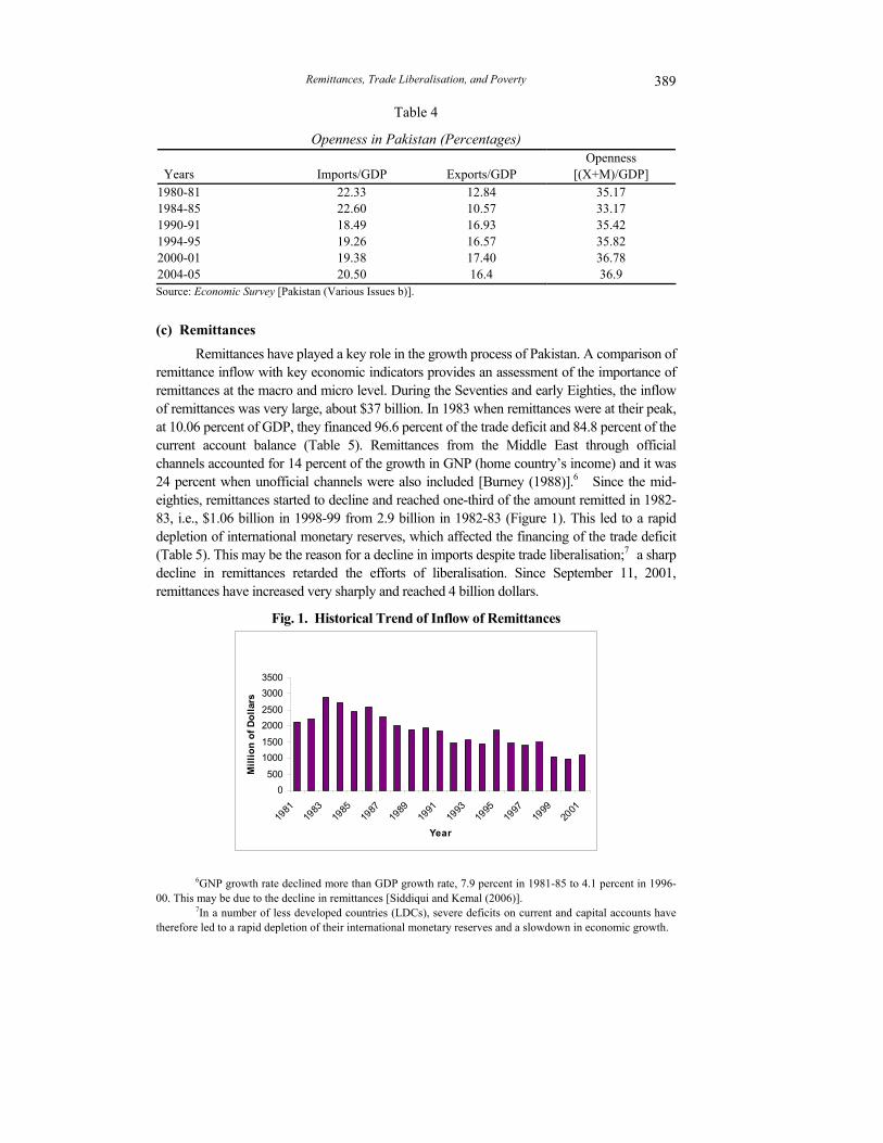
remittances at the macro and micro level. During the Seventies and early Eighties, the inflow

of remittances was very large, about $37 billion. In 1983 when remittances were at their peak,

at 10.06 percent of GDP, they financed 96.6 percent of the trade deficit and 84.8 percent of the

current account balance (Table 5). Remittances from the Middle East through official

channels accounted for 14 percent of the growth in GNP (home country’s income) and it was

24 percent when unofficial channels were also included [Burney (1988)].67 Since the mid-

eighties, remittances started to decline and reached one-third of the amount remitted in 1982-

83, i.e., $1.06 billion in 1998-99 from 2.9 billion in 1982-83 (Figure 1). This led to a rapid

depletion of international monetary reserves, which affected the financing of the trade deficit

(Table 5). This may be the reason for a decline in imports despite trade liberalisation;78 a sharp

decline in remittances retarded the efforts of liberalisation. Since September 11, 2001,

remittances have increased very sharply and reached 4 billion dollars.

Fig. 1. Historical Trend of Inflow of Remittances

Figure 1. Historical Trend of Inflow of Remittances

0

500

1000

1500

2000

2500

3000

3500

1981

1983

1985

1987

1989

1991

1993

1995

1997

1999

2001

Year

Mil

lio

n o

f D

oll

ars

6GNP growth rate declined more than GDP growth rate, 7.9 percent in 1981-85 to 4.1 percent in 1996-

00. This may be due to the decline in remittances [Siddiqui and Kemal (2006)]. 7In a number of less developed countries (LDCs), severe deficits on current and capital accounts have

therefore led to a rapid depletion of their international monetary reserves and a slowdown in economic growth.

Siddiqui and Kemal

390

Table 5

Contribution of Remittances in Key Economic Indicators (Percentages)

Financing through Remittances of

Years Current Account

Balance

Trade

Deficit

Remittances/

GDP

Remittances/

Private

Consumption

1980-81 67.11 76.56 7.53 9.98

1982-83 84.81 96.55 10.06 13.33

1985-86 67.74 85.31 8.14 10.67

1990-91 45.98 74.43 4.06 5.94

1995-96 24.20 39.44 2.26 3.13

2000-01 53.6 71.4 1.5 1.89

2004-05 52.1 67.3 3.7 4.50

Source: Economic Survey [Pakistan (Various Issues b)].

In addition to financing of imports at the national level, remittances have also

played an important role at the micro level. Migrants remit a significant amount to

Pakistan, on average 78 percent of their total earnings, and thereby increase the income

of households. Studies by Burney (1988) and Kazi (1988) indicate that remittance

income have been used for current consumption, retiring of debt or for repair of

houses.89 The importance of remittances at the household level can be gauged from the

fact that remittances were 13 percent of private consumption expenditure. Since 1982-83,

the ratio (Remittances to Private Consumption) has shown a declining trend, i.e., 13.3

percent in 1982-83 declining to 1.9910percent in 2000-01. The decline in remittance

income of households may be an important reason for the rise in poverty in Pakistan

during the Nineties. Empirical studies indicate that remittances improve the

recipients’ standard of living. Migrant workers from Pakistan, on average, received

incomes five to eight times higher than they received from employment in their home

country, remitting on average 78 percent of their earnings [Burney (1988)].

Therefore, a reduction in the flow of remittances is expected to have a dual impact on

poverty. First, it reduces the impact of trade liberalisation by limiting the inflow of

imports. Second, it reduces the income, as well, as consumption of households.

Figure 2 shows that remittance inflow increased during 1970-83 and declined

thereafter till 2000. After September 11, 2001, remittance inflow increases

significantly.

(d) Poverty

Poverty has increased irrespective of the choice of the measures of poverty;

head count, gap, and severity index [Mehboob-ul-Haq Centre for Human

Development (1999)]. It has increased in Pakistan during the Nineties (adjustment

period) compared to in the Eighties (pre-adjustment period). Table 6 presents

8Remittances are not utilised significantly to enhance the capital stock. At the sector level, the only

sector, which appears to have benefited from the inflow of remittances, in terms of increased private

investment, is ownership of dwellings. 9To some extent the decline in remittances at the household level is understated. The remittances were

also received through the hundi system.

Remittances, Trade Liberalisation, and Poverty

391

absolute poverty based on a basic need poverty line and Table 7 presents relative

poverty based on a poverty line of 75 percent of average income in the country.

Table 6 shows that the number of poor has increased from 29.2 percent in 1987-88

to 35.7 percent in 1993-94 and declined in 1999. The other two ratios, poverty gap

and severity index, also show that poverty has increased during the adjustment

period. The relative poverty measured by head count ratios increases from 45.6

percent population to 51 percent over 1987-88 to 1993-94 period. The other two

indicators, income gap and severity index, increased from 25.9 percent to 31

percent and 4.4 percent to 7.1 percent over the same period of time, respectively.

Table 6

Poverty Indicators Basic Need Approach (Based on Distribution of Income)

Pre-adjustment Post-adjustment

Measure

(Percent) Area 1986-

87

1987-

88

1990-91* 1992-93 1993-94 1998-

99**

2004-

05

Head Count Pakistan 28.6 29.2 29.4 35.9 35.7 32.6 35.7

Urban 28.8 28.9 31.3 29.7 29.9 24.2 –

Rural 28.1 30.1 29.1 39.1 37.3 35.9 –

Income Gap Pakistan 20.6 21.1 26.3 28.9 27.9 7.0 –

Urban 21.2 21.7 25.5 26.6 24.1 5.0 –

Rural 20.2 20.1 26.1 28.3 27.5 7.9 –

Severity Index Pakistan 1.8 1.9 3.1 4.5 4.1 1.51 –

Urban 1.9 2.0 3.2 3.4 2.8 2.51 –

Rural 1.7 1.9 3.0 4.8 4.2 2.2 –

Source: Mehboob-ul-Haq Centre for Human Development (1999). *Poverty lines for the year 1990-91 for

Pakistan, rural and urban areas are 276.7, 257.6 and 307.9 Rs respectively. **World Bank (2002) For

the income gap ratio, they use percentage in total.

Table 7

Relative Poverty Indicators for Pakistan, Urban and Rural Areas

Pre-adjustment

Period

During Adjustment

Period

Measure (Percent) Area 1986-87 1987-88 1990-91* 1992-93 1993-94

Head Count Pakistan 47.5 45.6 52.9 51.6 51.0

Urban 52.5 49.3 57.0 54.2 53.5

Rural 38.6 37.9 49.6 46.5 43.0

Income Gap Pakistan 25.9 25.3 33.1 33.0 31.6

Urban 27.8 26.9 33.4 33.2 32.1

Rural 22.7 22.2 32.1 30.3 28.6

Severity Index Pakistan 4.4 4.1 7.9 7.8 7.1

Urban 5.5 4.9 8.6 8.2 7.4

Rural 2.9 2.7 7.0 6.2 5.1

Source: Mehboob-ul-Haq Centre for Human Development (1999). *Poverty Line = 75 Percent of the Average

Income (Based on Distribution of Income) Poverty lines for the year 1990-91 for Pakistan, rural and urban

are 388, 348 and 441 rupees respectively.

Siddiqui and Kemal

392

III. REVIEW OF LITERATURE

A number of empirical studies1011have analysed the impact of trade liberalisation

based on the Stolper-Samuelson theorem—one of the central results of the Heckscher-Ohlin

theory. The studies analyse the change in poverty and welfare when a country is moving

from autarky to free trade. These studies demonstrate how changes in output prices caused

by changes in tariffs translate into the change in the prices of the factors of production with

positive production and zero economic profit condition. Convergence in relative prices of

the factors of production1112may reduce inequality through increased demand for labour, the

most abundant factor in developing countries like Pakistan. However, the empirical results

are very sensitive to the country sample, time period and specification of the model. The

Stolper-Samuelson theorem suggests that the per capita income differentials due to

existing factor endowment differentials tend to disappear over time after trade

liberalisation [Krugman and Obstfeld (1994)]. The change in the relative prices of goods

together with a change in income affects households’ consumption. Tariff reductions

reduce import prices and benefit consumers by supplying cheap consumer goods.

Depending on the elasticity of substitution, in presence of trade liberalisation, consumers

start to substitute imports for domestically produced goods. Consequently, the demand

for domestic goods falls and domestic prices decline further.

Bourguignon, de Melo, and Suwa (1989) show that devaluation that is pro-trade helps

the poor in the low income countries as it encourages export-oriented industries, which

employ more workers. On the other hand, import rationing worsens inequality because the

rationing premium accrues to capitalists. Clarete and Whalley (1988) explore the ways in

which trade policies and other domestic distortions interact in the small open developing

economy. Using a price-taking open economy numerical general equilibrium model of the

Philippines, they report that in the presence of import quota and rent-seeking activities, tariff

removal makes the country worse off. Another model with special emphasis on distributional

issues is developed by Dervis, de Melo, and Robinson (1982) for three archetype economies.

They suggest that the distributional implications of an external shock depend on the initial

structure of the economy and the choice of adjustment policies.

Decaluwe, et al. (1999) and Cockburn (2002) explicitly incorporate poverty and

income distribution in a CGE framework. Decaluwe, et al. (1999) developed a beta-

distribution based approach on the basis of parameters chosen according to the

characteristics of households and a basic need poverty line determined by quantity of

basic need commodities. The change in monetary value of the poverty line with the

change in prices is determined endogenously in the model. The study shows that a

reduction in tariffs is beneficial to the alleviation of poverty. Cockburn (2002) analyses

the impact of trade liberalisation on poverty using micro simulation. He argues that trade

liberalisation can only be properly analysed in a CGE model with disaggregated

household data, and developed a model for Nepal incorporating all households from a

nationally representative household survey. He emphasises that complex income and

consumption effects could not be analysed in an aggregate CGE model. Using the micro

simulation method, the study shows that urban poverty falls and rural poverty rises and

income inequality increases with the rise in income.

10Guisinger and Scully (1991), Decaluwe, et al. (1999), Siddiqui and Iqbal (1999), Cockburn (2002),

Kemal, et al. (2002), etc. 11Stolper-Samuelson theorem of price equalisation.

Remittances, Trade Liberalisation, and Poverty

393

The literature related to the “impact of remittances on poverty” explains how the

recipients typically use remittances and how they affect economic indicators in the country.

Studies show that remittances are mainly used for current consumption; the rest is spent on the

maintenance of dwellings. During the large inflow of remittances, investment in ownership of

dwellings increases by a higher percentage [Burney (1988)]. Migrants who belong to the low-

income class before migration save less and spend more on current food and consumer

durables as compared with medium and high-income groups. Another study by Kruijk (1987)

exploring the sources of income inequality points out that, in addition, to labour and property

income, exogenous factors like migration to the Middle East had played a very important role

in reducing poverty during the mid-Seventies and early Eighties.1213The direct and indirect

effects of remittances suggest remittances are beneficial for trade in goods and

services,1314income growth, and contribute to savings (though a negligible amount).

Therefore, it can safely be concluded that remittances can (and do) make important

contributions to welfare enhancing and poverty reduction. During the Nineties, remittances

have declined sharply in Pakistan, it may be the major factor giving rise to poverty.

Fig. 2. Poverty and Inflow of Remittances (Percentages)

R E M /G D P P P P R P U

REM/GDP—Ratio of Remittances to GDP

PP—Poverty in Pakistan, PR—Poverty in Rural area, PU—Poverty in Urban area

IV. DATA AND METHODOLOGY

A consistent data set for the year 1989-90, using the Input-Output table for

1989-90 [Pakistan (1996)], Household Integrated Economic Survey (HIES) [Pakistan

(1993)] and SAM 1989-90 [Siddiqui and Iqbal (1999a)], is constructed. Production

activities in agriculture, mining, manufacturing and services are classified on the

basis of their characteristics viz. import competing and exporting orientations.

Agriculture is subdivided into the crop and non-crop sectors. The manufacturing

sector is aggregated into five activities: food, textiles, chemicals, machinery and

other manufacturing. The services sector is classified into three activities, two

12See Irfan (1997), Amjad and Kemal (1997) and Usman, et al. (2000). 13In addition to providing money for basic needs such as food, clothing, housing improvements, and

education, it provides hard currency for consumer goods such as small household appliances.

60

50

40

30

20

10

0

Per

cen

tag

e

1965 1970 1875 1980 1985 1990 1995 2000 2005

Year

Siddiqui and Kemal

394

tradable and one non-tradable sector. The main characteristics of these sectors are as

follows: The crop sector provides raw material for exports in particular to the textile

industry, the major export supplying sector accounting for 67 percent of total

exports. ‘Chemicals’ and ‘Machinery’ are the major import competing sectors and

the rest of the sectors have mixed characteristics. The imports account for 30.9

percent and 55.6 percent of the expenditure on chemical and machinery, respectively.

The shares of imports of these sectors in the overall imports of the country are 18.4

percent and 37.5 percent, respectively [Siddiqui and Kemal (2006)].

Earlier studies show that a large percentage of remittance income accrues to poor

households as 81 percent of migrants belong to production workers and only 19 percent

to the professionals. Social Accounting Matrix (SAM) 1989-90 provides information on

the sources of household income by income groups. In this study, we classify households

by occupation in urban and rural areas as the two areas present different levels of poverty.

They are aggregated by occupation of head of households into five categories;

professionals, clerks, agriculture skilled workers, production worker and miscellaneous.

We identify five sources of household income;1415labour, capital, dividends from firms,

transfers from government and transfers from the rest of the world. The first three sources

of income are endogenously determined in the model. The distribution of remittance

income across the households is fixed in the model. Therefore urban households who

receive a larger share of remittances 77 percent of remitted income, experienced larger

negative effects of a decline in remittances.

Table 8

Sources of Income for Rural and Urban Households (Percentages)

Wages Capital Dividends

Transfers from

Government Remittances Total

Professional 59.46 24.23 14.81 0.41 1.09 100

Clerks 28.53 38.41 18.86 0.31 13.88 100

Agriculture

Worker 13.01 76.42 0.00 0.16 10.41 100

Production

Worker 51.52 34.38 5.15 0.18 8.78 100

Miscellaneous 23.52 63.58 1.72 1.72 9.47 100

Urban Total 33.99 45.96 9.40 0.71 9.95 100

Professional 19.18 80.48 0.00 0.05 0.29 100

Clerks 38.95 56.53 0.01 1.45 3.06 100

Agriculture

Worker 13.82 81.55 0.43 2.27 1.93 100

Production

Worker 56.77 31.22 3.75 0.98 7.29 100

Miscellaneous 16.97 54.37 19.22 4.57 4.87 100

Rural Total 26.51 63.61 4.40 2.09 3.40 100

Source: Social Accounting Matrix, 1989-90.

14Income refers to total receipts.

Remittances, Trade Liberalisation, and Poverty

395

Table 8 reports the share of households’ incomes from different sources. In the urban

sector, professionals receive 59.5 percent of their income and production workers receive

51.5 percent of their income from labour. The other three groups in the urban area receive

higher percentage from capital. All households in the rural area receive a higher percentage

of their income from capital except production workers who receive 56.8 percent of their

income from labour. In the urban households, the share of remittances in total household

income ranges from 1 percent to 14 percent and mean level is 9.95 percent. In the rural area,

it ranges 0.3 percent to 7.3 percent with mean of 3.4 percent. It needs to be underscored that

the share of remittances in the incomes of professional groups, who are relatively rich in

both the urban and rural area is only 1.0 percent and 0.2 percent of their total income,

respectively. On the other hand, urban households—clerks—receive 35.8 percent of

remittances. In the rural area, production workers receive 8.43 percent of remittances (Table

9). Both types of households are relatively poor and 31.5 percent and 36.3 percent of

households, respectively, are below the poverty line (Table 9).

Table 9

F-G-T Indicators of Poverty and Remittances Share (Percentages)

Base Year (Pα-Measures)

Households by

Occupation Households

Head

Count

Poverty

Gap

Severity

Index

Share of

Remittances

Professional 2.71 19.92 4.68 1.15 0.92

Clerks 14.91 31.52 3.77 2.42 35.76

Agriculture Worker 2.12 35.33 7.43 1.44 5.06

Production Worker 13.83 40.08 5.51 1.26 13.62

Miscellaneous 7.11 23.44 9.39 3.25 21.92

Urban Total 40.68 32.44 7.27 2.36 77.28

Professionals 9.07 25.2 5.2 1.42 0.22

Clerks 2.37 34.25 7.38 2.33 3.31

Agriculture 11.56 28.3 6.43 2.12 4.68

Production Worker 22.29 36.3 7.31 2.22 8.41

Miscellaneous 14.03 23.19 4.58 1.41 6.09

Rural Total 59.32 30.47 6.49 2.05 22.72

Source: Social Accounting Matrix, 1989-90.

Using the above-mentioned consistent data set, the computable general

equilibrium (CGE) model is used to simulate the impact of tariff reduction and the

decline in remittances. The model is similar in many respects to the CGE model

developed for the MIMAP-project, which has been developed to analyse the impact of

trade liberalisation on welfare and poverty1516in Pakistan. The main characteristics of the

model are discussed below.

In the neo-classical framework, this model contains six blocks of equations; income

and saving, production, foreign trade, demand, prices, and market equilibrium. The model

has four institutions: households, firms, government and rest of the world. The ownership

15For details see Siddiqui and Iqbal (1999b) and Siddiqui, et al. (2006).

Siddiqui and Kemal

396

of factors of production and their returns determine factor income. All wage income

accrues to households, as they own all labour. In addition, households receive income in

the form of remittances from the rest of the world, transfers from firms as dividends and

transfers from government as social security benefits. Transfers from government and

rest of the world are exogenous. The effect on income of households due to trade policy

shock is determined through changes in the endogenous sources of income: wage income,

capital income, and dividends from firms. The household’s dividend income is defined as

fixed share from the firms’ capital income. After subtracting income tax from the

household’s total income, we get the disposable income of the household. Household

savings are defined as a fixed share of households’ disposable income. The second

institution—the firm receives income from two sources; receipts from capital and

transfers from the government. The firm’s capital income is defined by subtracting the

sum of the household’s capital income from production activities. Transfers from the

government to firms are given exogenously. Its expenditure includes tax payments to the

government, dividends to households, and transfers to the rest of the world. Subtracting

all these from the firm’s income, savings of the firms are calculated. The third institution,

government receives tax revenue from various sources; international trade, production,

households’ income and tax on capital income of the firms. These five types of taxes

endogenously determine government revenue. In addition, the government also receives

transfers from the rest of the world, which are fixed exogenously. Subtracting transfer

payments to households and firms and government consumption expenditure from

government revenue we get government savings. The fourth institution is the rest of the

world. Its income includes income from sales of imports and transfers from firms, and

outlay includes expenditure on exports, remittance income to households and transfers to

government.

Domestic production has eleven sectors—ten tradable and one non-tradable.1617All

production activities employ factors of production; labour and capital. Labour is assumed

to be homogeneous and mobile across the sectors, while capital is sector-specific.

Production functions are specified by a technology in which gross output has separable

production function for value added and intermediate inputs. Leontief technology

between intermediate and output and within intermediates is assumed. The value added is

defined by the Constant Elasticity of Substitution (CES) production functions. Assuming

perfect competition and market clearing conditions, labour demand function for ith sector

is derived from the Constant Elasticity of Substitute (CES) production function. Returns

to capital are determined by the zero profit condition.

Goods for the domestic market and for foreign market (exports) with the same

sector classification are of different qualities. The Constant Elasticity of Transformation

(CET) function describes the possible shift between domestic and external markets.

Domestically produced goods sold in the domestic market are imperfect substitutes for

imports (Armington assumption). The import aggregation function presents demand for

composite goods (imported and domestically produced goods). For non-traded goods,

total demand is equal to total domestic supply. Profit maximisation or cost minimisation

gives desired exports supply and imports demand functions of relative prices (domestic to

foreign prices). The equilibrium in the foreign market is determined with inflow and out

16For detail see Siddiqui and Kemal (2006).

Remittances, Trade Liberalisation, and Poverty

397

flow of goods and transfers across the border. Nominal exchange rate and current account

balance are given exogenously, while the real exchange rate is implicit in the model.

Keeping the CAB and nominal exchange rate constant, real exchange rate depreciate

leading to cheap exports.

In the model, we have four types of demand for goods and services: household

consumption, government consumption, intermediate inputs, and demand for goods for

investment purposes. Total household consumption is defined as residual after

subtracting saving from disposable income. Household demand is specified by the linear

expenditure system (LES). It is derived from maximising a Stone-Geary utility function

subject to the household’s budget constraint.1718Using the Frisch parameter1819and income

elasticities, which are given in the model exogenously; we derive the minimum

consumption of a good by a household group. Government expenditure includes

expenditure on goods and services, transfers to households, and transfers to firms.

Government current expenditure on the ith commodity is derived by Cobb-Douglas utility

function and is defined as fixed share in total expenditure. The private and public

consumption are aggregated to get total consumption expenditure. The sum of input

requirements by the production sector for each commodity produced determines

intermediate demand for the ith commodity. Demand for goods for investment purposes

is the fixed value share in total investment.

For welfare analysis, we fixed total demand for investment and government

consumption in real terms so that increase in welfare may not be at the expense of

government consumption or investment. We deflate current investment demand by its

deflator and get investment in real terms. Deflating current government expenditure

with its deflators gives government consumption in real terms.

The model contains different prices associated with each good. We retain the small

country assumption. World prices of exports and imports are given. Domestic price of

exports and imports are defined after including taxes, if any. Imports are restricted

through tariff barriers and sales tax is also imposed on imported goods. Producer price is

the weighted average of the domestic price of goods for the domestic market and the

domestic price of goods for the export market. There is a sales tax on all goods, so

domestic price is determined after including taxes. Consumer prices are the weighted

average of domestic price and import price of the nth commodity for traded goods and for

non-tradables it is equal to the domestic price. GDP deflator (Pindex) is the weighted

price index of all goods. The two deflators for investment goods and government

consumption are defined as the weighted average of all commodities.

The final block presents equilibrium conditions. Total investment is equal to total

domestic saving and foreign savings. Total consumption expenditure on the ith good is

the sum of expenditures by different household groups and government, intermediate use

by different production activities and demand for investment purposes. Walras’ law

holds. Total labour demand is equal to labour supply, which is given exogenously. We

use the external sector closure rule in the model. We assume price-taking behaviour for

exports as well as for imports in the international market1920i.e., world export price and

world import price are exogenous to the model.

17Maximising u(X) = ∑fi (Xi) = ∑ αi −log(γi) subject to constraint ∑ PiXi = Y. 18For a detailed discussion of Linear Expenditure Systems, see Deaton and Muellbaur (1987). 19Small open economy assumption.

Siddiqui and Kemal

398

The model described above has been calibrated to the data of the Pakistan economy for

the year 1989-90. Policy parameters, all tax rates, savings rates are calculated from the base

year data. Shift and share parameters in the demand and supply equations, are also generated

from base year data. For the consumption function, household specific income elasticities for

each commodity are estimated from micro data from the Household Integrated Economic

Survey. Elasticities for import aggregation and export transformation functions are taken from

different studies.21 Elasticities for production function are taken from Kemal (1981) and

Malik, et al. (1989). The elasticities which were not available are fixed after discussion.

The study focuses on welfare and poverty outcome of policy shocks.

Equivalent variations (EV) are estimated to see the change in welfare of the

households. We use Foster, Greer, and Thorbecke (FGT) (1984) Pα measures for

poverty analysis, Where P0 measures the households below the poverty line, P1 measures

poverty gap and P2 measures severity of the poverty.2122 We use micro data from the

national representative Household Integrated Economic Survey [Pakistan (1993)] of

more than six thousand households. Basic need-poverty line is estimated on the basis

of adult equivalent calorie intake for the base year.2223 For the non-food items, we

take the average of the expenditure of the households’ two percentage points above

and below the food poverty line. The poverty lines are estimated separately for urban

and rural areas to eliminate the impact of price differentials between the regions.

Poverty estimates for the base year are given in Table 9. In urban and rural areas,

production workers are the poorest group of households, where 40.1 percent and 36.3

percent of households respectively live below the poverty line. Table 9 clearly shows that

the poor receive a higher percentage and rich households receive a lower percentage of

remittances. For example, clerks in the urban area receive 35.8 percent of remittances. In

the rural area, production workers’ share is highest, at 8.4 percent of remittances. The

other two groups, agriculture skilled workers and clerks can be classified as poor

households where about one-third of households are below the poverty line in both, urban

and rural areas. The professionals and miscellaneous groups are classified as rich

households (Table 9) in urban and rural areas. They receive only 0.9 percent and 0.2

percent of remittances, respectively.

For poverty change analysis,2324the real value of poverty (quantity) is kept fixed in

every simulation [see Decaluwe, et al. (1999)]. However, the poverty analysis approach

differ from Decaluwe, et al. (1999) in some aspects, it uses micro data from the HIES

instead of assuming β-distribution. The monetary value of the poverty line is obtained by

multiplying the product with their respective prices. If qi is the quantity and Pci is the

price for ith good then we define the monetary value of basic need poverty (BNPm) line

for the base year as follows:

BNPm = ∑ qio*Pcio

20For detail see Kemal, et al. (2002). 21Pα = 1/n Σ{(Z–Yι)/Z}α where n is total number of households, Z is basic need poverty line, Yι is

income and α = 0 for head count ratio, α = 1 for poverty gap measure and α = 2 measure the severity of

poverty. 22Detail is given in Ercelawn (1990) and Ravallion (1994). 23For detail see Decaluwe, et al. (1999).

Remittances, Trade Liberalisation, and Poverty

399

Prices are determined endogenously in the model. As prices rise or fall after the

simulation, the monetary value of the poverty line rises or falls as well. The change in

poverty line is determined as follows

∆BNPm = ∑ qio*Pci1 – ∑ qio*Pcio

Note: o indicates the base year and 1 indicates after the shock.

Changes in prices shift the poverty line and the change in income of the group

shifts the density function left or right depending on the negative or positive change in

income [Siddiqui, et al. (2006)]. These two changes determine the change in poverty after

the policy shock in the country. We calculated these poverty indicators before and after

the shocks. First, we simulate the impact of tariff reduction in the base year equilibrium.

Second, tariff and remittances are reduced simultaneously to see how the impact of trade

liberalisation changes in the presence of a decline in remittances.

The list of equations along with endogenous and exogenous variables is given

in Appendix A. The General Algebraic Modelling System (GAMS) software package is

used to solve and simulate the model.

V. SIMULATION RESULTS

The results of two simulation exercises are discussed here. First, a tariff cut on

imports by 55 percent is introduced in the model to examine the impact of trade

liberalisation on welfare and poverty keeping remittances constant. A reduction in trade

barriers has a two-fold impact on households: (1) a reduction in distortions in domestic

prices relative to world prices, results in a reallocation of resources from the protected

sectors to the unprotected sectors. In turn, it affects payments to factors of production. This

change in factor rewards results in a change in households’ incomes depending on their

ownership of the factors of production. (2) The consumer reallocates expenditure from

expensive goods (domestic goods produced by import competing sectors) to relatively

cheaper goods (imports) and reduces expenditure on domestically produced goods.

In the second exercise, we reduce remittances by 44 percent in the presence of

tariff reduction of 55 percent. A decline in remittances results in a decline in the income

of households depending on their share in remittances. The households, who receive

larger share of total remittances experience a larger negative effect of the decline in total

remittances i.e., 77 percent of total remittances, accrue to urban households. The decline

in income affects the household welfare. The tabulated results indicate reallocation of

resources, the change in factor rewards, household income and expenditure, welfare and

poverty in Pakistan in response to the policy shocks.

Simulation 1. Trade Liberalisation

In the first simulation, we reduce the tariff rate by 55 percent across the board on all

imports. Table 10 describes the effects on the macro economic variables. The reduction in the

tariff rate leads to a decline in the relative prices of all imports significantly except in the

mining and the other traded sectors—the unprotected sectors in the base year. The reduction

in protection reduces competitiveness of sectors and producers reduce their production and

Siddiqui and Kemal

400

shift resources towards unprotected sectors. Consumers substitute cheap imported goods for

the domestic goods that lead to a large inflow of total imports, i.e., a 4.5 percent increase over

the base year.

Depending on the elasticity of substitution and the share of imports in total

consumption in the base year, demand for all imports increases except in unprotected sectors:

mining and other traded (Table 10). The reduction in domestic costs caused by the tariff cut

increase the profitability of the export sectors. This leads to the expansion of output and

employment in the export sector notably in ‘textiles’.2425However, the increased inflow of

imports is by no means enough to eliminate the import competing sectors. Output declines

significantly in Chemical, Machinery and ‘Other Manufacture’ sectors by 2.8 percent, 2.0

percent and 2.0 percent, respectively (Table 10).

Increase in imports with fixed current account balance and nominal exchange rate lead

to depreciation of the real exchange rate, which boosts exports. The strength of this export

response depends on the fall in domestic prices, the capacity of local producers to

substitute between local and export markets, and initial export intensities. However, this

increase in exports is not fully compensated by the decline in domestic demand. Only the

crop and textile sectors show an increase in domestic production after the shock, 0.1

percent and 5.4 percent, respectively, indicating trade liberalisation benefits the export

sector of Pakistan more. Depending on the elasticity of substitution, elasticity of

transformation and share of imports and domestically produced goods in their respective

domestic demand, domestic demand for the textile sector increases by 3 percent.

The fall in output in a number of sectors leads to a decline in demand for factors of

production. Released factors of production from inefficient sectors, which are relatively more

protected, move towards efficient or unprotected sectors that are more productive. Resultantly,

labour demand increases in the export-oriented sectors ‘crop’ and ‘textile’ by 0.43 percent and

16.3 percent, respectively. Returns to capital increase in ‘Textile’ sector by 6.1 percent. The

expansionary effects in some sectors, mainly in export sectors cannot outweigh the

contraction effects in the import competing sectors, chemicals and machinery. Thus, both

returns to labour and capital (an index) decline by 0.5 percent and 1.5 percent, respectively

(Table 10). The results confirm the proposition that trade liberalisation affects more negatively

sector specific factors of production.

The significant disparity in poverty levels among the different groups of

households requires an investigation into the variation in the various income sources after

the policy shock. The reduction in factors prices, wages and returns to capital, by –0.51

percent and –1.5 percent have a negative impact on the household’s nominal income. The

production workers households suffer the least decline in income in the urban as well as

in the rural area, 0.85 percent and 0.81 percent respectively (Table 11). These are the

poorest group of households in their respective regions. This implies that trade

liberalisation is relatively less harmful for the poor. However, variation in change in

income across the income groups is not very significant.

The change in consumer prices affects the household specific consumer price

index (CPI). Table 11 shows that a decline in the CPI is larger than the decline in income

for each household group, that result in higher real income of households. This exercise

24Textile is a major exportable sector, i.e., textile sector exports are 67.7 percent of total exports and 44

percent of total output.

Table 10

Simulation Results: Variation Over Base Year Values (Percentages)

Sectors Imports Domestic Demand Exports Production

Domestic Price

Producer Price

Import Price Wage Rate

Returns to Capital

Consumer Price

Labour Demand

Trade Liberalisation (55 Percent Reduction in Tariff on all Imports)

Crop 1.05 0.08 2.07 0.10 –1.63 –1.62 –2.56 –0.5 –0.02 –1.66 0.43 Non-crop 34.87 –0.58 3.20 –0.38 –2.83 –2.68 –20.70 –0.5 –2.20 –3.30 –2.55 Mining –3.83 –1.20 1.83 –1.09 –3.70 –3.57 –1.51 –0.5 –4.33 –2.90 –3.47 Food 10.71 –0.64 4.07 –0.37 –3.04 –2.86 –11.39 –0.5 –2.68 –4.11 –1.75 Textile 13.47 3.01 8.34 5.41 –4.12 –2.26 –11.0 –0.5 6.06 –4.42 16.32 Chemicals 6.65 –2.94 4.35 –2.79 –4.71 –4.62 –11.37 –0.5 –12.04 –7.18 –9.39 Machinery 4.07 –2.04 5.43 –1.98 –6.96 –6.90 –12.32 –0.5 –6.81 –10.31 –5.72 Other Manufacturing 8.78 –2.27 6.17 –1.98 –5.37 –5.19 –12.85 –0.5 –8.34 –7.10 –5.58 Other Trade (Sector 1) –4.18 –0.50 3.36 –0.27 –3.66 –3.45 –0.03 –0.5 –2.21 –3.60 –1.55 Other Trade (Sector 2) –2.34 –0.81 0.93 –0.81 –1.92 –1.92 0 –0.5 –2.20 –1.56 –0.03 Non Traded Sector – – – –0.01 – –2.84 –9.99 –0.5 – –4.26 –1.2 Total* 4.50 –0.46 6.84 0.20 –3.39 –3.04 –0.5 –1.50

Trade Liberalisation in Presence of Decline in Remittances (Reduction in Tariff Rate by 55 Percent and Remittances by 44 Percent)

Crop –5.70 –0.94 8.35 –0.88 –7.20 –7.15 –2.56 –3.41 –7.58 –7.03 –3.9 Non-crop 22.05 –1.84 9.87 –1.21 –8.31 –7.85 –20.70 –3.41 –8.60 –8.62 –7.96 Mining –5.59 –0.64 4.06 –0.47 –5.62 –5.41 –1.51 –3.41 –5.02 –4.14 –1.5 Food 0.88 –2.69 11.53 –1.86 –8.69 –8.18 –11.39 –3.41 –13.53 –9.03 –8.48 Textile 8.57 6.92 21.24 13.49 –9.94 –5.35 –11.00 –3.41 11.96 –9.99 41.87 Chemicals 2.77 –3.14 8.42 –2.91 –7.24 –7.09 –11.37 –3.41 –15.04 –8.75 –9.76 Machinery 2.28 –1.64 8.17 –1.56 –8.90 –8.83 –12.32 –3.41 –8.26 –11.03 –4.53 Other Manufacturing 3.24 –2.98 11.01 –2.49 –8.59 –8.28 –12.85 –3.41 –12.88 –9.56 –6.97 Other Trade Sector 1 –8.53 –1.03 7.12 –0.55 –7.46 –7.02 –0.03 –3.41 –6.74 –7.35 –3.12 Other Trade Sector 2 –7.29 –2.74 2.64 –2.74 –5.81 –5.80 0.00 –3.41 –8.90 –4.74 0.07 Non Traded Sector – – – 0.03 – –5.50 –9.99 –3.41 – –7.85 –4.02 Total* 0.59 –0.92 17.13 0.75 –7.81 –6.87 –2.56 –3.41 –6.32 –7.03 –

Table 11

Variation in Income and Consumer Price Index of Households (Percentages)

Trade Liberalisation (55 Percent

Reduction in Tariff on all

Imports)

Trade Liberalisation in Presence of

Decline in Remittances (Tariff Rate by

55 Percent and Remittances

by 44 Percent)

Nominal

Income

Household

Consumer Price

Index

Nominal

Income

Household Consumer

Price Index

Urban Households

Professional –0.88 –3.45 –4.97 –7.29

Clerks –1.00 –3.44 –10.70 –7.66

Agriculture Worker –1.21 –3.46 –9.85 –7.86

Production Worker –0.85 –3.43 –8.12 –7.78

Miscellaneous –1.10 –3.44 –9.09 –7.35

Urban Total –1.00 –3.44 –9.03 –7.58

Rural Households

Professional –1.31 –3.42 –5.87 –7.92

Clerks –1.04 –3.40 –6.25 –7.94

Agriculture Worker –1.30 –3.25 –6.50 –7.95

Production Worker –0.81 –3.36 –7.35 –7.97

Miscellaneous –1.19 –3.47 –7.37 –8.06

Rural Total –1.16 –3.34 –6.70 –7.97

Pakistan Total –1.07 –3.39 –7.95 –7.77

shows, that with a given level of government expenditure and investment demand, trade liberalisation generates a welfare (equivalent variation) gain to every household group in the urban and rural areas. In urban areas, the welfare gain to the poorest household group (production worker) is not very different from the welfare gain to the relatively rich households (professionals), 2.69 percent and 2.68 percent, respectively. While in the rural areas, the welfare gains to the poorest (production worker) is the highest, 2.6 percent. The aggregate welfare gain is larger for urban households compared to rural households, at 2.6 percent and 2.3 percent, respectively (Table 12).

Siddiqui and Kemal

384

Table 12

Decomposition of Welfare Impact (Percentage Change)

Households by Socio Economic Groups

Trade Liberalisation

(55 Percent Reduction in Tariff on all

Imports)

Total Effect of Trade Liberalisation in Presence of

Decline in Remittances (Reduction in Tariff Rate

by 55 Percent and Remittances by 44 Percent)

Reduction in Remittance

Urban Households

Professional 2.69 2.50 –0.19

Clerks 2.60 –3.22 –5.82

Agriculture Worker 2.53 –2.05 –4.58

Production Worker 2.68 –0.38 –3.06

Miscellaneous 2.48 –1.85 –4.33

Urban Total 2.58 –1.56 –4.14

Rural Households

Professional 2.49 2.56 0.07

Clerks 2.39 1.77 –0.62

Agriculture Worker 2.00 1.56 –0.44

Production Worker 2.61 0.64 –1.97

Miscellaneous 2.39 0.77 –1.62

Rural Total 2.30 1.41 –0.89

Pakistan Total 2.45 –0.19 –2.64

The central issue in this study is to find the links between trade liberalisation and

poverty in Pakistan. The results show that the income of all households declines after the

shock of a tariff cut (Table 11). The density function (percentage of individuals with

given income) shifts to the left (Figures 3 to 12). This shift in the density function

increases the population below the poverty line (old) as more households move towards

the lower income bracket if the poverty line does not change. However the results show

that the value of the poverty line declines by 3.4 percent for urban households and by 3.3

percent for rural households due to change in consumer prices (Table 11). As a result, the

poverty line shifts to the left. The poverty line shift more than compensates for the fall in

income, which results in a reduction of the population below the poverty line in each

household group (Figures 3 to 12).

Table 13 presents quantitative estimates of FGT indicators (Pα-measures) for absolute

poverty; head count (Po), poverty gap (P1) and severity (P2). In the urban and the rural

areas, the head count ratio declines between 2.4 to 14.4 percent and 3.4 to 9.6

percent, respectively. The poverty gap and the severity indices have both declined in

all households in the urban as well as in the rural areas. From the table we may note

that trade liberalisation is more beneficial for urban households as all poverty

indicators (Pα-measures) decline more for households in the urban areas (who were

relatively poor before simulation) compared to the households in the rural area. We

can conclude that the policy shock benefits the poor.

Table 13

Changes in F-G-T Indicators of Poverty (Percentages) Head Count Gap Severity

Households

Base Tariff cut Tariff cut and

Decline in Remit-tances

Decline in Remit-tances

Base Tariff cut Tariff cut and

Decline in Remit-tances

Decline in Remit-tances

Base Tariff cut Tariff cut and

Decline in Remit-tances

Decline in Remit-tances

Professional 19.92 –9.64 2.66 12.30 4.68 –9.81 10.08 19.89 1.15 –9.57 11.30 20.87

Clerks 31.52 –7.30 6.85 14.15 3.77 –7.40 9.02 16.42 2.42 –9.50 11.57 21.07

Agriculture 35.33 –14.44 0.00 14.44 7.43 –12.89 3.09 15.97 1.44 –13.89 3.47 17.36

Production Worker 40.08 –7.09 4.92 12.00 5.51 –7.56 8.63 16.19 1.26 –8.62 10.15 18.77

Others 23.44 –2.35 3.71 6.06 9.39 –9.62 6.84 16.45 3.25 –11.90 9.52 21.43

Urban (Total) 32.44 –7.09 5.09 12.18 7.27 –7.98 8.39 16.37 2.36 –9.32 10.59 19.92

Professional 25.2 –3.57 –3.57 0.00 5.20 –8.46 –8.65 –0.19 1.42 –11.27 –11.27 0.00

Clerks 34.25 –3.42 –3.42 0.00 7.38 –7.86 –8.13 –0.27 2.33 –9.01 –9.01 0.00

Agriculture 28.3 –6.40 –5.55 0.85 6.43 –7.15 –6.22 0.93 2.12 –8.49 –8.02 0.47

Production Worker 36.3 –6.12 –5.92 0.19 7.31 –8.34 –8.62 –0.27 2.22 –9.46 –9.46 0.00

Others 23.19 –9.57 –9.14 0.43 4.58 –8.08 –8.30 –0.22 1.41 –9.22 –9.93 –0.71

Rural (Total) 30.47 –6.01 –5.61 0.39 6.49 –7.70 –7.55 0.15 2.05 –9.27 –8.78 0.49

Density Functions and Shift in the Density Functions after the Shock

(Urban Households)

Figure 3: Density Function

(Professional)

0

0.0002

0.0004

0.0006

0.0008

0.001

0.0012

-500 0 500 1000 1500 2000 2500

Income

De

nsity

Base Sim 1 Sim 2

Figure 4: Density Function

(Clerks)

-0.0005

0

0.0005

0.001

0.0015

0.002

0.0025

0.003

-500 0 500 1000 1500 2000 2500

Income

De

nsity

Base Sim 1 Sim 2

Figure 6: Density Function

(Production worker)

-0.0005

0

0.0005

0.001

0.0015

0.002

0.0025

0.003

0.0035

-500 0 500 1000 1500 2000 2500Income

Den

sit

y

Base Sim 1 Sim 2

`

Figure 5: Density Function

(Agriculture)

-0.0005

0

0.0005

0.001

0.0015

0.002

0.0025

0.003

0.0035

-500 0 500 1000 1500 2000 2500

Income

De

ns

ity

Base Sim 1 Sim 2

Figure 7: Density Function

(Miscellaneous)

0

0.0002

0.0004

0.0006

0.0008

0.001

0.0012

0.0014

0.0016

-500 0 500 1000 1500 2000 2500Income

De

nsity

Base Sim1 Sim2

Fig. 3. Density Function (Professional) Fig. 4. Density Function (Clerks)

Fig. 5. Density Function (Agriculture) Fig. 6. Density Function (Production Worker)

Fig. 7. Density Function (Miscellaneous)

Siddiqui and Kemal

384

Density Functions and Shift in the Density Functions after the Shock

(Rural Households)

Figure 8: Density Function

(Professionals)

0

0.0005

0.001

0.0015

0.002

0.0025

0.003

-500 0 500 1000 1500 2000 2500Income

De

ns

ity

Base Sim 1 Sim 2

Graph9: Density Function

(Clerks)

-0.0005

0

0.0005

0.001

0.0015

0.002

0.0025

0.003

0.0035

-500 0 500 1000 1500 2000 2500

Income

De

ns

ity

Base Sim 1 Sim 2

Figure 10: Density Function

(Agriculture )

-0.0005

0

0.0005

0.001

0.0015

0.002

0.0025

0.003

0.0035

-500 0 500 1000 1500 2000 2500

Income

Den

sit

y

Base Sim 1 Sim 2

Figure 11: Density Function

(Production Worker)

-0.0005

0

0.0005

0.001

0.0015

0.002

0.0025

0.003

0.0035

0.004

-500 0 500 1000 1500 2000 2500

Income

Den

sit

y

Base Sim 1 Sim 2

Figure 12: Density Function

(Miscellaneous)

-0.0005

0

0.0005

0.001

0.0015

0.002

0.0025

0.003

-500 0 500 1000 1500 2000 2500

Income

De

ns

ity

Base Sim1 Sim2

Fig. 8. Density Function (Professional) Fig. 9. Density Function (Clerks)

Fig. 10. Density Function (Agriculture) Fig. 11. Density Function (Production Worker)

Fig. 12. Density Function (Miscellaneous)

Remittances, Trade Liberalisation, and Poverty

385

For the analysis of distributive effects of liberalisation, we draw graphs for

variation in the density function for the urban and rural areas before and after a

change in government policy; tariff reduction. In Figures 13 and 14 Variation-1

shows that majority of households in the lower income group change their income

brackets i.e., households move from the middle-income bracket (500-1000) towards

the lower income bracket (250-500). There is a very little variation in the higher

income brackets. This suggests that the income disparity has increased after trade

liberalisation in the urban as well as in the rural areas of Pakistan. The overall results

show that absolute poverty has declined by all measures in Pakistan in the presence

of trade liberalisation. The empirical results on poverty contradict these findings as

poverty increases by all measures during the period of trade liberalisation (Table 6

and Table 7). In the next section we explore the other channels which may be the

cause of the rise in poverty in Pakistan during the 1990s.

Figure 14: Variation in Density Function

(Rural Households)

-0.0003

-0.0002

-0.0001

0

0.0001

0.0002

0.0003

0.0004

0.0005

0 500 1000 1500 2000 2500

Income

Dif

fere

nce

o variation variation 1 variation 2

Figure 13: Variation in Density Function

(Urban Househodls)

-0.0003

-0.0002

-0.0001

0

0.0001

0.0002

0.0003

0.0004

0.0005

0.0006

0 500 1000 1500 2000 2500

Income

Dif

fere

nc

e

o variation variation 1 variation 2

Fig. 13. Variation in Density Function (Urban Households)

Fig. 14. Variation in Density Function (Rural Households)

Siddiqui and Kemal

386

Simulation 2. Trade Liberalisation in the Presence of Decline in Remittances

In this section, the results of the combined shock to the economy of a reduction in tariffs

and a reduction in remittances are discussed. The tariffs and remittances are reduced

simultaneously by 55 percent and 44 percent, respectively, (the actual decline over the 1990-

2000). The cut in tariff reduces the domestic prices of all imports, which reduce competitiveness

of the sectors protected in the base period, 1990. The sectors where the tariff was high in the base

period i.e., non-crop, food, textiles, chemicals, machinery and other miscellaneous manufactured

imports show an increase in imports. However, the total increase in imports is less than one

percent compared to 4.5 percent in the first simulation. The decline in remittances restricts the

inflow of imports because imports are financed by foreign remittances. With the Current

Account Balance (CAB) constant, decline in remittances is partially compensated by a decline in

imports and partially by a larger increase in exports from each sector as the real exchange rate

depreciate. The exports from Pakistan increase by 17.1 percent compared to the increase in

exports of 6.8 percent in the previous exercise (Table 10).

Aggregate domestic demand for domestic goods decline by 0.9 percent compared

to decline in total demand for domestic goods, 0.46 percent in the previous exercise. The

larger decline can be attributed to decline in the remittance income of households. The

producer of exportable goods diverts a portion of his sales from the domestic to the

export market. The largest increase in exports is from textiles, which leads to an increase

in output from this sector. However, increase in the exports in all other sectors is not

equal to the decline in domestic demand in their respective sectors. Therefore, output fell

in those sectors. This leads to a reallocation of resources including factors of production.

The results show that demand for labour increases only in ‘textiles’ where

domestic production increases. All other sectors show a decline in labour demand. The

wage rate falls by 3.4 percent. Similarly, returns to capital increase only in the textile

sectors. The overall results show that returns to capital decline by 6.3 percent (Table 10).

If we compare the effects on macro variables in this and the previous exercise, it becomes

clear that a decline in remittances has reduced the gains of trade liberalisation.

The adverse impact of decline in remittances on households depends on the

households’ share in total remittances. In addition to the decline in remittances, the fall in

factor prices also has a negative impact on the households’ nominal income (Table 11).

Households’ income decline by 5 to 10 times higher than in the previous exercise due to

decline in remittances. In urban areas, the income of clerks declined by 10.7 percent, who

receive 35.8 percent of remittances. In rural areas, the decline in income is between (–5.9

percent) to (–7.4 percent). The least decline is in the income of rich households

(professionals) who receive only 0.2 percent of remittances (Table 9 and Table 11).

In this simulation, import prices fell by the same amount as in the first simulation

but PD declined by a higher percentage due to reduction in household demand for goods

and services. Resultantly, consumer prices fell for all commodities by a larger amount in

this exercise (Table 11). The results show that rich households in urban and rural areas,

(professionals) still gain in terms of equivalent variation at 2.5 percent and 2.6 percent

respectively because, they are least affected through decline in remittance income. All

other households lose in the urban areas. In rural areas all other households groups also

gain but less than the rich households. However, the gain of trade liberalisation reduces

with a decline in remittances.

Remittances, Trade Liberalisation, and Poverty

387

Figures 3 to 12 reveal that a reduction in remittances in the presence of trade

liberalisation shifts the density curves to the left more than in the previous exercise. These

figures show that more households shift towards the lower income bracket in this exercise.

The area specific consumer prices index decline by 7.6 percent and 8.0 percent for the

urban and rural areas, respectively (Table 11). Resultantly, the poverty lines on the curves

also shift to the left. The shifts in the poverty lines are more than compensated for some

households, while for others the opposite is true. Households’ specific poverty effects (Pα-

measures) of trade liberalisation in presence of the decline in remittances are presented in

Table 13. In urban areas, households below the poverty line increase in all household

groups except for those, in the agricultural group of households. In rural areas, the head

count ratio declines for each group of households. This suggests that trade liberalisation still

benefits rural households in spite of the decline in remittances. An examination of the

poverty gap and poverty severity indicators, P1 and P2, gives the same message (Table 13).

Variation-2 in Figures 13 and 14 reveals distributive effects of liberalisation in the presence

of a decline in remittances. The figures show a movement of households from the middle-

income bracket (500-1000) towards lower income brackets is very large in this simulation.

This suggests that a decline in remittances enhanced the adverse distributive impact of trade

liberalisation. Income disparity increased due to the remittance decline.

Decomposition Analysis

A comparison of the results from the two exercises of the tariff cut and decline in

remittance on welfare and poverty in Pakistan shows that trade liberalisation through tariff

cuts increases the welfare of urban and rural households compared with the base year. But

trade liberalisation in the presence of a reduced inflow of remittances reduces the welfare of

urban households by 1.6 percent. However, rural households still gain in terms of welfare

by 1.4 percent (Table 12). The third column in the Table 12 shows that the decline in

remittances reduces welfare of each household in urban and rural households (except

professional households in rural areas who receive only 1 percent of remittances), this is

contrary to trade liberalisation effect where every household gains. The negative impact of

remittance decline on urban households (–4.14 percent) is larger than the negative impact

on rural households (–0.89 percent). In terms of total effects, the negative impact of

remittance dominates the positive impact of trade liberalisation for urban households. The

reverse is true for rural households as they still show a welfare gain.

Percentage changes in FGT-indicators for three effects: (1) tariff cut, (2) tariff cut and

decline in remittances, and (3) decline in remittances only are presented in Table 13. The table

shows that absolute poverty has declined in urban as well as in rural households because of trade

liberalisation. However, with the decline in remittances poverty rises according to all Pα-

measures in the both areas, urban and rural. The results of trade liberalisation in the presence of a

decline in remittances shows that remittance impact dominates for urban households, but trade

liberalisation impact dominates for rural households in terms of the total effect.

VI. CONCLUSION

The paper explores the contribution of trade liberalisation policies and decline in

remittance income of households to welfare and poverty in Pakistan. It analyses the impact of

Siddiqui and Kemal

388

trade liberalisation through tariff cut in the absence and the presence of decline in remittances

on welfare and poverty in a CGE framework. Trade liberalisation boosts exports and benefits

most the export-oriented labour-intensive sector, textiles. It is relatively more harmful to the

sector specific factor of production, capital. The gains are larger for urban households than for

rural households in terms of both welfare enhancement and poverty reduction. The study

comes out with the conclusion that a tariff cut is welfare inducing and poverty reducing and

trade liberalisation is not the cause of the rise in poverty in Pakistan during the 1990s.

In the second set of experiments, trade liberalisation in the presence of a decline in

remittances reduces the gains of trade liberalisation. It reduces the welfare of urban

households over the base year. Although rural households still show an increase in welfare

over the base year, but less than the welfare gain with trade liberalisation only. According

to all FGT indicators, poverty increases in urban households but not in rural households.

This shock hurts more the relatively poorer group of households, clerks and production

workers, who receive the major share of remittances.

Decomposition of impact of trade liberalisation and decline in remittances show

explicitly that poverty increases according to all poverty measures in rural and urban areas

of all households from a decline in remittances. However, the negative impact of remittance

decline dominates the positive impact of trade liberalisation in urban areas and the positive

impact of trade liberalisation dominates the negative impact of a decline in remittances in

the rural area. We conclude from this that the decline in remittance inflows is a major

contributory factor in explaining the rise in poverty in Pakistan. Trade liberalisation

increases income inequality. Decline in remittances reinforces this impact.

APPENDIX A

COMPUTABLE GENERAL EQUILIBRIUM MODEL FOR PAKISTAN

A. Foreign Trade Statistics

1. [ ] Tn

Tnn

Tn

Tn

Tnn

Tsn DEXBX ρρρ δ−+δ= /1)1( Export Transformation (CET)

2. sn

sn

sn

nsn

sn

snn DMBQ

ρρρ− δ−+δ= /1])1([ Constant Elasticity of Substitution

between Imports and Domestic

Goods

3. XQ NTNT = Domestic Demand for Non-traded

Goods

4. [ ] nT

nT

nD

nE

nn DPPExtn

Tn */)1()/(

σσ δδ−= Export Supply

5. [ ]nnnM

nD

nn DPPMSn

Sn *]1/(()/(

σσ δ−δ= Import Demand

6.

CAB*eTR

TREX*PTR/e)(*MP

RG

RHnWE

nFRnWM

n

=−

−−+ ∑∑ 1 Equilibrium in Foreign Market

B. Income and Saving

7. * GHRHHiiKHDi

wlHH TRTReDIVKRLY +++λ+λ= ∑∑ Households’ Income

8. *Y dvr DIV FKHH = Dividend, Income from Firms

9. HYyhtYDH

*)1( −= Households Disposable Income

10. HHH YDapsS * = Households’ Saving

11. ∑= HH S TS Total Households’ Saving

Remittances, Trade Liberalisation, and Poverty

389

12. ∑ ∑λ−= )()1( iikFK KRY Firms’ Capital Income

13. GFFKF TRYY += Firms’ Total Income

14. ∑ −−−= FKkHFRFF YtDIVTRYS * Firms’ Saving

15. Siiii XPtxTXS **= Taxes on Production

16. n

WM

nnn MPetmTXM **= Taxes on Imports

17. n

WM

nnn XPeteTXE **= Taxes on Exports

18.

∑∑∑

++Τ

∗ +++ ∗∑=

nnRG

iFKHHG

TXETXMR

eTXSYtkYtyY *)( Government Revenue

19. ∑∑ −−−= GiGHGFGG CTRTRYS Government Saving

C. Structure of Production C

20. ii

Si ioICX /= Output

21. )(*)( ii XiioIC = Intermediate Consumption from

ith sector

22. jjiij ICaICJ = Intermediate Demand of ith sector

from jth

23. ii

Diiiiii LKBVA σ−σ−σ δ−+δ= /1]))(1([ Production Function (CES)

24.ii

i

iDi KwRL *}/}{

)1({ 1/1

δ

δ−= +ρ Labour Demand

25. /)**( iDii

VAii KLwVAPR −= Return to Capital

D. Demand

26. HHH SYDCT −= Total Households Consumption

27. ∑−+== ici

ichhi

cicii )}/PγP(CTβ γ{ P (h)C Households demand function (LES)

28. ciGii PCTCG /Γβ= Government Consumption

29.iHii CGCTC += ∑ Total Private and Public

Consumption

30. jiji ICaINTD ∑= Intermediate Demand

31. ci

Iii PITI /*β= Investment Demand

32. gGir PCTCG /= Government Total consumption in

Real term

E. Prices

33. WMnn

Mn PetxtmP **)1(*)1( ++= Domestic Price of Imports

34. WEnn

En PeteP **)1( += Domestic Price of Exports

35. ) *P EX * D (Pt XPE

iis

iiSii += Producer Price

36. ∑−= ) IC(P ) *X (P *VAP jic

is

iiiVA

i Value Added Price

37. ) tx * ( Pt PD iii += 1 Domestic Price after paying taxes

38. Mnnn

Dnnn

Cn ) P /Q (M )* P /Q (D P += Composite Price of traded goods

(consumer prices)

39. PD P ntC

nt = Composite Price of non-traded

goods

Siddiqui and Kemal

390

40. ) * P(β Pindex iX

i∑= GDP Deflator

41. P PgIi

gI

ci ββΠ= )/( Deflator for Government

Consumption

42. IiI

iC

iI PPββ∏= )/( Deflator for Investment

F. Equilibrium

43. CAB*eSSTSIT FGH +++= ∑ Saving-Investment Equilibrium

44. I INTD C Q i iii ++= Commodity Market Equilibrium

45. )(L LD

iS ∑= Labour Market Equilibrium

VARIABLES

Endogenous Variables

1. Ci Total Consumption of ith Good 42. YFK Firms Capital Income

2. CGi Government final Consumption of Good i Exogenous Variables

3. CTG Total Government Consumption 1. CAB Current Account Balance

4. CHi Household Consumption of Good i 2. CTGR Government final consumption in real

terms

5. CTH Total Household Consumption 3. e Nominal Exchange Rate

6. Di Domestic Demand for domestically

produced good

Ki ith Branch Capital Stock

7. DIVH Dividends distributed to Households from

firms

5. LS Total Labour Supply

8. EXn Exports of nth good (FOB) 6. PnWE World Price of Exports

9. ICi Total Intermediate Consumption of Good

by ith sector

7. PnWM World Price of Imports

10. ICij Intermediate Consumption of Good J by ith

sector

8. TRFR Firms transfers to the rest of world

11. INTDI Intermediate Demand of Good I 9. TRGF Government transfers to Firms

12. Ii Consumption of Good for investment in

sector ith sector

10. TRGH Government Transfers to Households

13. IT Total Investment 11. TRRG Foreign transfer payments to the

Government

14. LiD Labour Demand in sector i 12. TRRH Foreign transfers to Households

15. Mn Imports of nth good (CAF) SYMBOLS

16. Pg Price deflator for government consumption 1.

Symbols

Variable Names

17. PI Price Deflator for Investment 2. aij Input Output Coefficients

18. Pi Producer Price 3. Bi CES scale parameter of value added

19. Pti Domestic price without taxes 4. BeT CET scale parameter of Import aggregation

function

20. PiC Price of Composite good 5. Bc

s CES scale parameter of export

transformation function

21. PnD Price of domestically produced and

consumed good including taxes

6. βhic Percentage share of good i in hth household

consumption

22. PnE Domestic price of Exports including all

taxes

7. βiG Percentage share of good i in Public

consumption

23. PnM Domestic Price of Imports including all

taxes

8. βiI Percentage share of good i consumed for

investment purposes

24. PnVA Value Added Price 9. βi

x Percentage share of good i in total

Production

25. PINDEX Producer price Index 10. γi Subsistence expenditure by hth household

Remittances, Trade Liberalisation, and Poverty

391

Endogenous Variables Symbols

26. Qi Domestic Demand for Composite Good i 11. λlH Household Share of Labour Income

27. Ri Rate of Return on capital in branch n 12. λkH Household Share of Capital Income

28. S G Government Saving (Fiscal Deficit) 13. ioI Leontief technical coefficients

(Intermediate Consumption of good i

29. SH Saving of Household h

30. SF Firms Savings 14. mpsh Household marginal propensity to save

31. TSH Total Households Savings 15. tk Capital Income tax rate of firms

32. TXEn Taxes on Exports of nth sector 16. σi CES elasticity of substitution of value

added

33. TXMn Taxes on Imports of nth sector 17. ρi CES Substitution parameter of value added

34. TXSi Indirect taxes on ith sector production 18. δi CES Distributive share of value added

35. VAi Value Added of sector i 19. σeT CET elasticity of transformation of export

36. W Wage rate 20. ρTe CET Substitution parameter of export

transformation

37. Xis Production of ith sector (Supply) 21. δT

e CET Distributive share of exports and

domestic production

38. YH Total Income Household h 22. σSc CES elasticity of substitution of imports

39. YDH Disposable income of Household h 23. ρSc CES Substitution parameter of imports

40. YF Firms total income 24. δSc CES Distributive share of imports and

domestically produced goods

41. YG Government Revenue

REFERENCES

Amjad, Rashid, and A. R. Kemal (1997) Macro Economic Policies and Their Impact on

Poverty Alleviation in Pakistan. The Pakistan Development Review 36:1, 39–68.

Bourguignon, F., J. de Melo, and A. Suwa (1989) Distributional Effects of Adjustment

Policies: Simulations for Two Archetype Economies. World Bank. (Background

Paper for 1990 World Development Report.)

Burney, Nadeem (1988) A Macro-Economic Analysis of the Impact of Workers’

Remittances from the Middle East on Pakistan’s Economy. (Working Paper No 8.

ILO-UN Project.)

Clarete, Ramon L., and John Whalley (1988) The Interactions between Trade Policies

and Domestic Distortions in a Small Open Developing Country. Journal of

International Economics 24, 345–358.

Cockburn, John (2002) Trade Liberalisation and Poverty in Nepal, A Computable General

Equilibrium Micro Simulation Analysis. Canada: CREFA, Université Laval Québec.

Deaton, A., and J. Muellbauer (1987) Economics and Consumer Behaviour. UK:

Cambridge University Press.

Decaluwe, Bernard, A. Party, L. Savard, and E. Thorbecke (1999) Poverty Analysis

Within a General Equilibrium Framework. CREFA 99-06. (Working Paper No. 9909.)

Dervis, K., J. de Melo, and S. Robinson (1982) General Equilibrium Models for

Development Policy. Washington, D. C.: The World Bank.

Ercelawn, A. (1990) Absolute Poverty in Pakistan: Poverty Lines, Incidence, Intensity.

Applied Economic Research Centre, University of Karachi. (Draft Paper).

Foster, J. Greer, and E. Thorbecke (1984) A Class of Decomposable Poverty Measures.

Econometrica 52:3, 761–766.

Siddiqui and Kemal

392

Guisinger, S., and G. Scully (1991) Pakistan. In D. Papageorgious, M. Michaely, and A.

M. Choksi (eds.) Liberalising Foreign Trade: The Experience of Indonesia, Pakistan,

and Sri Lanka. Vol. 5. Cambridge: Basil Blackwell.

Irfan, Mohammad (1997) Emigration from Pakistan–1947-97. Unpublished Report.

Pakistan Institute of Development Economics, Islamabad.

Kazi, Shahnaz (1988) Domestic Impact of Remittances and Overseas Migration:

Pakistan. ILO, UN. (Working Paper No 7.)

Kemal, A. R. (1981) Substitution Elasticities. In the Large-scale Manufacturing

Industries of Pakistan. The Pakistan Development Review 20:1,

Kemal, A. R., Rehana Siddiqui, and Rizwana Siddiqui (2001) Tariff Reduction and

Income Distribution: A CGE-based Analysis for Urban and Rural Households in

Pakistan. Pakistan Institute of Development Economics, Islamabad, Pakistan.

(MIMAP Technical Paper Series No 11.)

Kemal, A. R., Z. Mahmood, and A. M. Ahmad (1994) Structure of Protection, Efficiency,

and Profitability. Vol. 1. 1–134.

Khan, A. R. (1997) Globalisation, Liberalisation and Equitable Growth: Some Lessons for

Pakistan from Contemporary Asian Experience. The Pakistan Development Review

36:4, 915–928.

Krugman, R. Paul, and M. Obstfeld (1994) International Economics, Theory and Policy.

(Third Edition.) Harper Collins College Publishers.

Kruijk, H. de (1987) Sources of Income Inequality in Pakistan. The Pakistan Development

Review 26:4, 659–670.

Mahmood, Zafar (1999) Pakistan Conditions Necessary for the Liberalisation of Trade and

Investment to Reduce Poverty. Unpublished Research Paper.

Malik, S. J., M. Muhammad, and Hina Nazli (1989) An Analysis of Production Relations

in the Large Scale Textile Manufacturing Sector in Pakistan. The Pakistan

Development Review 28:1.

Mehboob-ul-Haq Centre for Human Development (1999) A Profile of Poverty in Pakistan.

United Nation Development Programme.

Pakistan, Government of (1993) Households Integrated Economic Survey. Islamabad:

Federal Bureau of Statistics.

Pakistan, Government of (1996) Supply and Use Tables of Pakistan, 1989-90. Islamabad:

Federal Bureau of Statistics.

Pakistan, Government of (Various Issues a) CBR Year Book. Islamabad: Central Board of

Revenue.

Pakistan, Government of (Various Issues b) Economic Survey. Islamabad: Finance

Division, Economic Advisors Wing.

Ravallion, M. (1994) Poverty Comparisons. Fundamentals of Pure and Applied

Economics. Vol. 56, Chur, Switzerland: Harwood Academic Publisher.

Siddiqui, Rehana, Rizwana Siddiqui, and Zafar Iqbal (1999) The Impact of Tariff Reforms

on Income Distribution in Pakistan: A CGE-Based Analysis. The Pakistan Development

Review 38:1, 789–804.

Siddiqui, Rizwana, and A. R. Kemal (2006) Poverty Reducing or Poverty Inducing? A

CGE Based Analysis of Foreign Capital Inflows in Pakistan. Pakistan Institute of

Development Economics, Islamabad. (PIDE Working Paper No. 2.)

Remittances, Trade Liberalisation, and Poverty

393

Siddiqui Rizwana, A. R. Kemal, Rehana Siddiqui, V. Robichaud, and M. A. Kemal

(2006) Tariff Reduction, Fiscal Adjustment and Poverty in Pakistan: A CGE-based

Analysis. The study completed under MIMAP-Project Phase II.

Siddiqui, Rizwana, and Zafar Iqbal (1999a) Social Accounting Matrix of Pakistan for

1989-90. Pakistan Institute of Development Economics, Islamabad, Pakistan.

(Research Report No. 171.)

Siddiqui, Rizwana, and Zafar Iqbal (1999b) Tariff Reduction and Functional Income

Distribution in Pakistan: A CGE Model. Pakistan Institute of Development Economics,

Islamabad. (Research Report No. 10.)

Siddiqui, Rizwana, A. R. Kemal, Rehana Siddiqui, Veronique Robichand, and M. A.

Kemal (2006) Tariff Reduction, Fiscal Adjustment and Poverty in Pakistan: A CGE-

based Analysis. A study completed under MIMAP Project- Phase II.

Usman, Q., M. A. Kemal, and Hasan M. Mohsin (2000) Impact of Trade Reforms on

Poverty. The Pakistan Development Review 39:4, 1127–1137.

World Bank (1989) Growth through Adjustment. Washington, D. C.: The World Bank.

World Bank (2002) Poverty in Pakistan in the 1990s: An Interim Assessment (Draft Report).