religious participation effects on mental and
TRANSCRIPT

RELIGIOUS PARTICIPATION EFFECTS ON MENTAL AND PHYSICAL
HEALTH
A Dissertation
Presented to the Faculty of the Graduate School
of Cornell University
In Partial Fulfillment of the Requirements for the Degree of
Doctor of Philosophy
by
Jennifer A. Nolan
January 2006

© 2006 Jennifer A. Nolan

RELIGIOUS PARTICIPATION EFFECTS ON MENTAL AND PHYSICAL
HEALTH
Jennifer A. Nolan, Ph.D.
Cornell University 2006
The first section of the dissertation provides a review of the literature, conceptual
distinctions between religiousness and spirituality, and four key hypothesized
pathways identified and categorized from the literature, posited to explain the effects
of religious participation on health.
The second section investigates the relationship of religious participation to physical
health, mental health and depression and the mediating behavioral pathway of
cigarette and alcohol use. The study focuses on a sample of 2,102 individuals
followed from 1979 to 2000, utilizing data from the National Longitudinal Survey of
Youth 79 (NLSY79). The main findings are the following. Cross-sectional analysis
revealed a positive U-shaped relationship between religious attendance and physical
health in the year 2000, controlling for sociodemographic variables of gender, race,
marital status, education, number of children living in a household, work amount, and
income. Attendance levels of once per week to infrequent were related to better
physical health scores. Attendance among individuals of low socio-economic status
(SES) was associated with better physical health compared with no attendance.
African Americans reported better mental health and lower depression scores with
higher attendance levels compared to no attendance; Caucasians showed the opposite
trend. Examining the data longitudinally from 1982 to 2000, early attendance in young
adulthood was found to be positively associated with better mental health and less
depression in mid-adulthood, controlling for key sociodemographic variables. The

behavior of cigarette smoking frequency was a mediator between the relationship of
religious attendance and depression, controlling for key sociodemographic variables.
Alcohol abuse/dependency and heavy drinking showed evidence of mild mediation.
Attendance in young adulthood was protective against alcohol abuse/dependency,
heavy drinking and smoking in mid-adulthood.
In addition, the dissertation includes the development of a framework for future
qualitative analysis of exploratory interviews with professionals at international
humanitarian organizations on how religious beliefs and practices of a targeted
population are taken into account in health projects. Major themes explored are
conceptualizations of religiousness, spirituality and health, theorized mediating
pathways, field experiences and institutional policies.
Overall this research provides evidence to support the relationship between religious
participation and mental health, depression and physical health.

iii
BIOGRAPHICAL SKETCH
Jennifer A. Nolan received her B.A. from Amherst College, in Amherst Massachusetts
in 1992, with a major in Biology and concentration in Art History. From 1992 to 1994
she was a research assistant in the Biology Department at Amherst College. In 1997,
she completed a M.S. at the University of Massachusetts at Amherst School of Public
Health, with a major in Epidemiology and completed a master’s thesis in psychosocial
epidemiology. From 1997 to 2003, she was an instructor at the State University of
New York College at Cortland, in the Department of Health Sciences and Health
Education. Her Ph.D. was earned from the field of Policy Analysis and Management
in the College of Human Ecology from Cornell University, Ithaca, New York, with a
major in health and evaluation, and minors in epidemiology, human development,
public policy, and research methods. During her graduate work, she conducted
research and field experiences abroad with international humanitarian organizations in
the areas of health and education. She also studied coursework in religion and
spirituality at the Gregorian University and the University of St. Thomas, in Rome,
Italy.
This research was born from many years of interest in religion and science,
particularly in the shared common purpose of these paradigms for understanding the
world and our place in it, as well as the inevitable tensions between these two
paradigms. This topic has been nurtured by family and many inspiring and challenging
instructors and friends along the way. The author looks forward to the surprises,
challenges and discoveries in future research endeavors.

iv
I dedicate this work to my brother and sister
James and Maureen
and to my parents
Helen and Michael Nolan
for their unconditional love and encouragement
to dream and live life to the fullest.

v
ACKNOWLEDGMENTS
This work was initiated, created and completed because of the shared vision, belief,
strength and support of many people. This present work is a testament to this fact, and
perhaps one of the most important lessons learned from this process.
I acknowledge my parents for their belief, encouragement, support, and continual
limitless sacrifices. I acknowledge my sister Rosemary and my brothers Michael,
Patrick, Kevin, and Brian, who have been inspiring, always challenging and
supportive.
I extend great appreciation to my chair, Eunice Rodriguez, who has encouraged and
nurtured this interest into a viable dissertation project and future research career.
Without her outstanding and caring mentorship, encouragement, and patience, this
entire research project would have been impossible. She is a rare and remarkable
model as a woman academic for the quality of her scholarship, her international
perspective, and her professional and personal integrity and strength. I am appreciative
of my chair’s support, focused guidance and wisdom, more than words could express.
I also extend much appreciation to Jerome Ziegler, who has also challenged me to
pursue this topic with enthusiasm and critical and provoking thought. He is a wise
mentor as an academic and as a person. He has instilled deep reflections on the
meaning of “quality of life” for the individual and humanity. I consider him a guru of
life, learning, courage and the responsibility to make a difference. The impact that
these two mentors, Eunice Rodriguez and Jerome Ziegler, have had on me is not
something I can yet fully understand or express, nor do I think I am to know fully at

vi
this time. Though I carry their impact with me, this impact will no doubt manifest
itself in unforeseen and positive ways.
I thank Elaine Wethington for her encouragement in the pursuit of this topic, for her
expertise in psychosocial epidemiology, and for her mentorship throughout my
graduate studies. I thank Lindy Williams for first exposing me to qualitative research
and for her mentorship, caring and good humor. I am also appreciative of Liz Peters,
who has been very supportive as a field director of graduate studies during my time at
Cornell.
Steve McClaskie at the National Longitudinal Study User Services and Jay Zagorsky
at the Center for Human Resource Research, Ohio State University have both been
invaluable with clarifications and nuances concerning the dataset.
I am appreciative of the generosity and honesty of the interviewees in sharing their
professional and personal views on this topic. They have been incredibly generous
with their time, experiences and reflections on the topic of socio-cultural beliefs and
practices and health within an international humanitarian context.
Innumerable people along the way have provided encouragement, guidance, insight
and lively discussion on this topic and the research process. I thank Professors Ben
Wodi, Ray Goldberg, and Anthony Papalia, my former mentors at the State University
of New York College at Cortland, for their encouragement and belief in me as I have
pursued graduate studies. I particularly would like to thank Geysa Smiljanic, the PAM
Graduate Field Assistant, for her support. I thank Karen Grace-Martin and Simona
Despa at the Statistical Consulting Office at the College of Human Ecology for their

vii
statistical expertise, as well as the statistical advice of Professor Steven Schwager of
the Department of Biological Statistics and Computational Biology.
I would also like to thank Joanne Button at Uris Library and Kristen Ebert-Wagner for
their expertise in the formatting and presentation of the document.
For their lively discussions, support and good humor I thank fellow present and former
graduate students, especially Jennifer Cowan, Laura Colosi, Naomi Penny, David
Abrahams, Monica Ruiz-Cesares, and Jennifer Jabs. I thank my friends Joanne
Rainbow-Wafer and Helen H. Buckley whose friendship, encouragement and spiritual
support have been invaluable.
I would like to acknowledge my appreciation of Cornell University funding sources
for the research: the Department of Policy Analysis and Management, the College of
Human Ecology, the Einaudi Center for International Studies, and the Graduate
School. I extend acknowledgement and appreciation for the Dr. Nuala McGann
Drescher United University Professions New York State Faculty Award for leave to
pursue the doctoral degree while an instructor at the State University of New York
College at Cortland.
Much gratitude to Ezra Cornell for his foresight in founding a great university in 1865
with the motto “I would found an institution where any person can find instruction in
any study.” This motto has allowed me to pursue with delight interdisciplinary studies
at Cornell.

viii
This research has not only challenged me academically but in countless other ways,
particularly in broadening my conceptualizations of religion, health and science. I look
forward to continuing the exploration of this topic and the insights, challenges and
adventures which invariably ensue from this research.

ix
TABLE OF CONTENTS
BIOGRAPHICAL SKETCH.....................................................................................iii DEDICATION .......................................................................................................... iv ACKNOWLEDGMENTS..........................................................................................v TABLE OF CONTENTS .......................................................................................... ix LIST OF FIGURES..................................................................................................xii LIST OF TABLES ...................................................................................................xx CHAPTER 1 Introduction The Effects of Religious and Spiritual Beliefs and Practices on Mental and Physical Health ...................................................................1
Motivation for this Research ..................................................................................1 Importance and Relevance of the Research............................................................1 Goal and Objectives of the Dissertation.................................................................2 Goal ........................................................................................................................2 Specific objectives and their rationale....................................................................3
CHAPTER 2 Literature Review of Dissertation The Influence of Spiritual and Religious Beliefs and Practices on Health: Key theoretical pathways for explaining the effects of religious and spiritual factors on health, with a focus on mental health....................................................................................................................................5
Background and Justification .................................................................................5 Brief Overview Epidemiology of Religion: A new emerging field .......................5 Religion/Religiousness versus Spirituality Conceptualizations .............................6 Mental Health: Background on Prevalence and Contribution to Global Burden of Disease..................................................................................................................13 Effects of Religious Factors on Mental Health: Summaries of Findings.............16 Effects of Religious Factors on Physical Health: Summaries of Findings...........22 Negative Effects of Religious Beliefs and Behavior on Health ...........................22 Epidemiological Constructs or Theoretical Framework for Understanding Religion’s Effect on Health—A New Theoretical Framework is Required.........31 Causal Mechanisms that Explain Religion’s Effects on Health ...........................32
CHAPTER 3 Objectives and Methods Quantitative Study Relationship between religious attendance and physical and mental health and depression among adults, explored cross-sectionally, over time, and through the mediating pathway of behavior, utilizing the National Longitudinal Survey of Youth 79 (NLSY79)........37
Objectives of the Study ........................................................................................37 Overview of Chapter ............................................................................................40 Background on National Longitudinal Survey of Youth Study ...........................40 Selection of this Study Sample from the Health Module 2000 ............................42 Overall Sample Design and Screening of the NLSY79 .......................................43 Stratification of Overall Sample of the NLSY79 .................................................45 Interview of Overall Sample of the NLSY79.......................................................45 Change in Overall Sample through Time and Retention Rates............................46 Potential Sources of Selection Bias......................................................................47 Weights.................................................................................................................48 Power....................................................................................................................49

x
Multicollinearity ...................................................................................................50 Statistical Software...............................................................................................50 Objective I. Cross-Sectional Analysis of the Relationship between Religious Attendance and Physical and Mental Health and Depression in the Year 2000, Among Those Aged 40 and Over. ........................................................................50 Details of Descriptions of Dependent and Independent Variables Used in the Analysis ................................................................................................................52 Objective II The Influence of Early Adulthood Religious Attendance in 1982 on Physical and Mental Health and Depression in Mid-Adulthood in 2000.............56 Objective III Test for Mediation of the Relationship between Early Adulthood Religious Attendance (1982) on later Health Status (2000) by Cigarette Smoking and Alcohol Dependency .....................................................................................59 Description of Potential Mediator Variables........................................................64
CHAPTER 4 Objective I Results .............................................................................68 Demographics of the Sample Population .............................................................68 Objective I Results ...............................................................................................88 Discussion Section Objective I...........................................................................121 Study Strengths...................................................................................................125 Study Limitations ...............................................................................................125 Possible Policy Implications...............................................................................126 Future Recommendations:..................................................................................127
CHAPTER 5 Objective II Results ..........................................................................128 Results Objective II The Influence of Religious Attendance, Affiliation, and Change in Attendance in early Adulthood on Mental Health, Depression, and Physical Health in Later Adulthood ...................................................................128 Overview of Chapter ..........................................................................................128 Sociodemographics of the Sample Population ...................................................128 Objective II Results The Influence of Religious Attendance, Affiliation, and Change in Attendance in early Adulthood on Physical Health, Mental Health, and Depression in Later Adulthood ..........................................................................156 Conclusion: Summary of Objective II................................................................199 Discussion of Objective II ..................................................................................200
CHAPTER 6 Objective III Results.........................................................................205 Results for Objective III Test for Mediation by Lifestyle and Behaviors of Alcohol Dependency (1994) and Cigarette Smoking Frequency (1994) on The Relationship between Religious Attendance (1982) in Early Adulthood and Physical Health, Mental Health, and Depression in mid-Adulthood (2000)......205 Overview of Chapter ..........................................................................................205 Descriptives of Behavior and Lifestyle Factors .................................................205 Mediators of alcohol abuse or dependency, heavy alcohol drinking, and frequency of cigarette smoking of the relationship between young adulthood religious attendance and mid-adulthood physical health, mental health, and depression ...........................................................................................................212 The Effects of Religious Attendance on later Alcohol Abuse or Dependency, Heavy Alcohol Drinking, and Cigarette Smoking Frequency............................223

xi
Conclusion: Summary of Objective III ..............................................................233 Increasing religious attendance in young adulthood is a protective factor against alcohol abuse or dependency, and frequency of heavy drinking and smoking. .233 Objective III Discussion .....................................................................................233
CHAPTER 7 Qualitative Framework The health effects of religious and spiritual beliefs and practices within international humanitarian projects: conceptualization, theory, mediating pathways, practice and policy ...................................................237
Introduction ........................................................................................................237 Justification for Qualitative Research ................................................................238 Objectives and Methods .....................................................................................238 Interview Content Themes .................................................................................239 Sample Selection ................................................................................................241 Confidentiality....................................................................................................241 Human Subject Approval ...................................................................................241 Qualitative Research Description .......................................................................242 Methods ..............................................................................................................242 Summary.............................................................................................................244
CHAPTER 8 Conclusion of Dissertation ...............................................................245 Summary of Findings from the Three Sections of Literature Review, Quantitative Analysis and the Qualitative Framework ......................................245 Literature Review and Key Pathways ................................................................245 Quantitative Analysis .........................................................................................246 Qualitative Exploration ......................................................................................250 Study Strengths and Other Studies’ Findings.....................................................251 Study Limitations ...............................................................................................254 Future Recommendations...................................................................................257 Possible Policy Implications of the Research.....................................................258
APPENDIX A: Quantitative Results: Objective One ................................................ 260 APPENDIX B: Objective II ....................................................................................... 288 APPENDIX C: Quantitative Results: Objective III ................................................... 314 REFERENCES........................................................................................................... 322

xii
LIST OF FIGURES Figure 3.1 Model of Mediating Pathway to Help Explain the Relationship of Religiousness on Mental and Physical Health Outcomes. ...........................................61 Figure 3.2 Model of Religiousness Effect on Physical Health, Mental Health and Depression. ...................................................................................................................62 Figure 4.1 Obj. I. Simple Model. Physical Health Composite Score (SF-12 PCS) in 2000 by Religious Attendance in 2000 controlling key sociodemographic variables in 2000 (as listed in Table 4.1: gender, race/ethnicity, marital status, education, children living in the household, work amount in 1999 and net family income in 1999)..........90 Figure 4.2 Obj. I. Simple Model. Mental Health Composite Score (SF-12 MCS) in 2000 by Religious Attendance in 2000 (controlling for socio-demographic variables in 2000 of gender, race/ethnicity, marital status, education, children living in household, work amount in 1999, net family income in 1999, residence and region). ..................97 Figure 4.3 Obj. I. Simple Model. CES-Depression in 2000 by Religious Attendance in 2000 (controlling for sociodemographic variables in 2000 of gender, race/ethnicity, marital status, education, children living in household, work amount in 1999, net family income in 1999, residence and region). ..........................................................101 Figure 4.4 Obj. I. Simple Model for Hispanics: Mental Health Composite Score (SF-12 MCS) in 2000 by Religious Attendance in 2000 (controlling for socio-demographic variables in 2000 of gender, marital status, education, children living in household, work amount in 1999, net family income in 1999, and residence..............................110 Figure 4.5 Obj. I. Simple Model for African Americans: Mental Health Composite Score (SF-12 MCS) in 2000 by Religious Attendance in 2000 (controlling for sociodemographic variables in 2000 of gender, marital status, education, children living in household, work amount in 1999, net family income in 1999, and residence).....................................................................................................................................111 Figure 4.6 Obj. I. Simple Model for Caucasians and all others: Mental Health Composite Score (SF-12 MCS) in 2000 by Religious Attendance in 2000 (controlling for gender, marital status, education, children living in household, work amount in 1999, net family income in 1999, and residence).......................................................112 Figure 4.7 Obj. I. Simple Model for Hispanics: CES-Depression Score (CES-D) in 2000 by Religious Attendance in 2000 (controlling for sociodemographic variables in 2000 of gender, marital status, education, children living in household, work amount in 1999, net family income in 1999 and region). .......................................................118 Figure 4.8 Obj. I. Simple Model for African Americans: CES-Depression Score (CES-D) in 2000 by Religious Attendance in 2000 (controlling for sociodemographic variables in 2000 of gender, marital status, education, children living in household, work amount in 1999, net family income in 1999 and region). .................................119 Figure 4.9 Obj. I. Simple Model for Caucasians and all others: CES-Depression Score (CES-D) in 2000 by Religious Attendance in 2000 (controlling for sociodemographic variables in 2000 of gender, marital status, education, children living in household, work amount in 1999, net family income in 1999 and region). 120 Figure 5.1 One-Way ANOVA of Physical Health Composite Score (SF-12 PCS) in 2000 by Change in Religious Attendance 1982 to 2000 without controls. ................153

xiii
Figure 5.2 One-Way ANOVA, of Mental Health Composite Score (SF-12 MCS) in 2000 by Change in Religious Attendance 1982 to 2000 without controls. ................154 Figure 5.3 One-Way ANOVA, of CES-Depression Score (CES-D) in 2000 by Change in Religious Attendance 1982 to 2000 without controls. ...........................................155 Figure 5.4 Obj. II. Simple Model of Physical Health Composite Score (SF-12 PCS) 2000 by Religious Attendance 1982 (controlling for baseline health limitations in amount or kind of work one could do for pay in 1981 and sociodemographic variables in 1982 of gender, race/ethnicity, marital status, education, number of children living in the household, work amount in 1981, net family income in 1981, residence and region).........................................................................................................................161 Figure 5.5 Obj. II. Simple Model of Mental Health Composite Score (SF-12 MCS) 2000 by Religious Attendance 1982 (controlling for baseline health limitations in amount or kind of work one could do for pay in 1981 and sociodemographic variables in 1982 of gender, race/ethnicity, marital status, education, number of children living in the household, work amount in 1981, net family income in 1981, residence and region).........................................................................................................................162 Figure 5.6 Obj. II. Simple Model of CES-Depression Score (CES-Depression) 2000 by Religious Attendance 1982 (controlling for baseline health limitations in amount or kind of work one could do for pay in 1981 and sociodemographic variables in 1982 of gender, race/ethnicity, marital status, education, number of children living in the household, work amount in 1981, net family income in 1981, residence and region).....................................................................................................................................163 Figure 5.7 Obj. II. Simple Model of Physical Health Composite Score (SF-12 PCS) by Religious Attendance 1982 (excluding baseline health limitations in amount or kind of work one could do for pay in 1981 and controlling for sociodemographic variables in 1982 of gender, race/ethnicity, marital status, education, number of children living in the household, work amount in 1981, net family income in 1981, residence and region).........................................................................................................................168 Figure 5.8 Obj. II. Simple Model of Mental Health Composite Score (SF-12 MCS) by Religious Attendance 1982 (excluding baseline health limitations in amount or kind of work one could do for pay in 1981 and controlling for sociodemographic variables in 1982 of gender, race/ethnicity, marital status, education, number of children living in the household, work amount in 1981, net family income in 1981, residence and region).........................................................................................................................169 Figure 5.9 Obj. II. Simple Model of CES-Depression Score (SF-12 CES-D) by Religious Attendance 1982 (excluding baseline health limitations in amount or kind of work one could do for pay in 1981 and controlling for sociodemographic variables in 1982 of gender, race/ethnicity, marital status, education, number of children living in the household, work amount in 1981, net family income in 1981, residence and region).........................................................................................................................170 Figure 5.10 Obj. II. Simple Model of Physical Health Composite Score (SF-12PCS) 2000 by Religious Affiliation 1982 (controlling for baseline health limitations in amount or kind of work one could do for pay in 1981 and sociodemographic variables in 1982 of gender, race/ethnicity, marital status, education, number of children living

xiv
in the household, work amount in 1981, net family income in 1981 and residence and region).........................................................................................................................178 Figure 5.11 Obj. II. Simple Model of Mental Health Composite Score (SF-12 MCS) 2000 by Religious Affiliation 1982 (controlling for baseline health limitations in amount or kind of work one could do for pay in 1981 and sociodemographic variables in 1982 of gender, race/ethnicity, marital status, education, number of children living in the household, work amount in 1981, net family income in 1981 and residence and region).........................................................................................................................179 Figure 5.12 Obj. II. Simple Model of CES-Depression Score (CES-D) 2000 by Religious Affiliation 1982 (controlling for baseline health limitations in amount or kind of work one could do for pay in 1981 and sociodemographic variables in 1982 of gender, race/ethnicity, marital status, education, number of children living in the household, work amount in 1981, net family income in 1981 and residence and region).........................................................................................................................180 Figure 5.13. Obj. II. Simple Model of Physical Health Composite Score (SF-12 PCS) 2000 by Change in Religious Attendance from 1982 to 2000 (controlling for baseline health limitations in amount or kind of work one could do for pay in 1981 and sociodemographic variables in 1982 of gender, race/ethnicity, marital status, education, number of children living in the household, work amount in 1981, net family income in 1981 and residence and region)......................................................186 Figure 5.14. Obj. II. Simple Model of Mental Health Composite Score (SF-12 MCS) 2000 by Change in Religious Attendance from 1982 to 2000 (controlling for baseline health limitations in amount or kind of work one could do for pay in 1981 and sociodemographic variables in 1982 of gender, race/ethnicity, marital status, education, number of children living in the household, work amount in 1981, net family income in 1981 and residence and region)......................................................187 Figure 5.15 Obj. II. Simple Model of CES-Depression Score (CES-D) 2000 by Change in Religious Attendance from 1982 to 2000 (controlling for baseline health limitations in amount or kind of work one could do for pay in 1981 and sociodemographic variables in 1982 of gender, race/ethnicity, marital status, education, number of children living in the household, work amount in 1981, net family income in 1981 and residence and region)......................................................188 Figure 5.16 Obj. II. Model of Physical Health Composite Score (SF-12 PCS) 2000 One Two-Way Interaction of Change in Religious Attendance 1982 to 2000 with Baseline Health Limitations in Amount or Kind of Work One Could Do for Pay in 1981 (controlling for baseline health limitations in amount or kind of work one could do for pay in 1981 and controlling for sociodemographic variables in 1982 of gender, race/ethnicity, marital status, education, number of children living in the household, work amount in 1981, net family income in 1981 and residence and region). ..........191 Figure 5.17 Obj. II. Model of Physical Health Composite Score (SF-12 PCS) 2000 One Two-Way Interaction of Change in Religious Attendance 1982 to 2000 with Education in 1982 (controlling for baseline health limitations in amount or kind of work one could do for pay in 1981 and controlling for sociodemographic variables in 1982 of gender, race/ethnicity, marital status, education, number of children living in

xv
the household, work amount in 1981, net family income in 1981 and residence and region).........................................................................................................................192 Figure 5.18 Obj. II. Model of Physical Health Composite Score (SF-12 PCS) 2000 One Two-Way Interaction of Change in Religious Attendance 1982 to 2000 with the Number of Children Living in the Household (controlling for baseline health limitations in amount or kind of work one could do for pay in 1981 and controlling for sociodemographic variables in 1982 of gender, race/ethnicity, marital status, education, number of children living in the household, work amount in 1981, net family income in 1981 and residence and region)......................................................193 Figure 5.19 Obj. II. Model of Mental Health Composite Score (SF-12 MCS) 2000 One Two-Way Interaction of Change in Religious Attendance 1982 to 2000 with Race/Ethnicity (controlling for baseline health limitations in amount or kind of work one could do for pay in 1981 and controlling for sociodemographic variables in 1982 of gender, race/ethnicity, marital status, education, number of children living in the household, work amount in 1981, net family income in 1981 and residence and region).........................................................................................................................194 Figure 5.20 Obj. II. Model of CES-Depression Score (CES-D) 2000 One Two-Way Interaction of Change in Religious Attendance 1982 to 2000 with Baseline Health Limitations in Amount or Kind of Work One Could Do for Pay in 1981 (controlling for baseline health limitations in amount or kind of work one could do for pay in 1981 and controlling for sociodemographic variables in 1982 of gender, race/ethnicity, marital status, education, number of children living in the household, work amount in 1981, net family income in 1981 and residence and region)......................................196 Figure 5.21 Obj. II. Model of CES-Depression Score (CES-D) 2000 One Two-Way Interaction of Change in Religious Attendance 1982 to 2000 with Race/Ethnicity (controlling for baseline health limitations in amount or kind of work one could do for pay in 1981 and controlling for sociodemographic variables in 1982 of gender, race/ethnicity, marital status, education, number of children living in the household, work amount in 1981, net family income in 1981 and residence and region). ..........197 Figure 5.22 Obj. II. Model of CES-Depression Score (CES-D) 2000 One Two-Way Interaction of Change in Religious Attendance 1982 to 2000 with the Number of Children Living in the Household (controlling for baseline health limitations in amount or kind of work one could do for pay in 1981 and controlling for sociodemographic variables in 1982 of gender, race/ethnicity, marital status, education, number of children living in the household, work amount in 1981, net family income in 1981 and residence and region)......................................................198 Figure 6.1 Obj. III. Mediator of Alcohol Abuse or Dependency in 1994, for the Simple Model of CES-Depression Scores (CES-D) in 2000 by Religious Attendance in 1982 (controlling for baseline health limitations in the amount or kind of work one could do for pay in 1981, and sociodemographic variables in 1982 of gender, race/ethnicity, marital status, education, number of children living in the household, work amount in 1981, net family income in 1981, residence and region). ................219 Figure 6.2 Obj. III. Mediator of Heavy Alcohol Drinking in 1994, for the Simple Model of CES-Depression Scores (CES-D) in 2000 by Religious Attendance in 1982 (controlling for baseline health limitations in the amount or kind of work one could do

xvi
for pay in 1981, and sociodemographic variables in 1982 of gender, race/ethnicity, marital status, education, number of children living in the household, work amount in 1981, net family income in 1981, residence and region). ..........................................220 Figure 6.3 Obj. III. Mediator of Cigarette Smoking Frequency in 1994, for the Simple Model of CES-Depression Scores (CES-D) in 2000 by Religious Attendance in 1982 (controlling for baseline health limitations in the amount or kind of work one could do for pay in 1981, and sociodemographic variables in 1982 of gender, race/ethnicity, marital status, education, number of children living in the household, work amount in 1981, net family income in 1981, residence and region). ................221 Figure 6.4 Obj. III. Mediator of Cigarette Smoking Frequency in 1994, for the Simple Model of Mental Health Composite Scores (SF-12 MCS) in 2000 by Religious Attendance in 1982 (controlling for baseline health limitations in the amount or kind of work one could do for pay in 1981, and sociodemographic variables in 1982 of gender, race/ethnicity, marital status, education, number of children living in the household, work amount in 1981, net family income in 1981, residence and region).....................................................................................................................................222 Figure A.1 Obj. I. Model of Physical Composite Score (PCS) in 2000 with the One Two-way Interaction of Religious Attendance in 2000 with Education in 2000 (controlling for socio-demographic variables in 2000 of gender, race/ethnicity, marital status, education, number of children living in household, work amount in 1999 and net family income in 1999).........................................................................................268 Figure A.2 Obj. I. Model of Physical Health Composite Score (SF-12 PCS) in 2000 with the One Two-way Interaction of Religious Attendance in 2000 with Work Amount in 1999 (controlling for socio-demographic variables in 2000 of gender, race/ethnicity, marital status, education, number of children living in household, work amount 1999 and net family income 1999). ...............................................................269 Figure A.3 Obj. I. Model of Physical Composite Score (SF-12 PCS) in 2000 with the One Two-way Interaction of Religious Attendance in 2000 with Net Family Income in 1999 (controlling for key socio-demographic variables in 2000 of gender, race/ethnicity, marital status, education, number of children living in household, work amount in 1999 and net family income in 1999)........................................................270 Figure A.4 Obj. I. Model of Physical Health Composite Score (SF-12 PCS) in 2000 with the One Two-way Interaction of Religious Attendance in 2000 with Education in 2000 (in the presence of the Two-way interactions of religious attendance in 2000 with work amount in 1999 and religious attendance in 2000 with net family income in 1999; controlling for socio-demographic variables in 2000 of gender, race/ethnicity, marital status, education, number of children living in household, work amount 1999 and net family income 1999). .....................................................................................271 Figure A.5 Obj I. Model of Physical Health Composite Score (SF-12 PCS) in 2000 with the One Two-way of Interaction of Religious Attendance in 2000 with Work Amount in 1999 (in the presence of the Two-way interactions of religious attendance in 2000 with education in 2000 and religious attendance in 2000 with net family income in 1999; controlling for socio-demographic variables in 2000 of gender,

xvii
race/ethnicity, marital status, education, number of children living in household, work amount in 1999 and net family income in 1999)........................................................272 Figure A.6 Obj I. Model of Physical Health Composite Score (SF-12 PCS) in 2000 with the One Two-way Interaction of Religious Attendance in 2000 with Net Family Income in 1999 (in the presence of the Two-way interactions of religious attendance in 2000 with education in 2000 and religious attendance in 2000 with work amount in 1999; controlling for socio-demographic variables in 2000 of gender, race/ethnicity, marital status, education, number of children living in household, work amount in 1999 and net family income in 1999).........................................................................273 Figure A.7 Obj. I. Model of Mental Health Composite Score (SF-12 MCS) in 2000 with the One Two-way Interaction of Religious Attendance in 2000 with Race/Ethnicity (controlling for socio-demographic variables in 2000 of gender, marital status, education, number of children living in the household, work amount in 1999, net family income in 1999, and residence).................................................................278 Figure A.8 Obj. I. Model of Mental Health Composite Score (SF-12 MCS) in 2000 with the One Two-way Interaction of Religious Attendance in 2000 with Education in 2000 (controlling for socio-demographic variables in 2000 of gender, race/ethnicity, marital status, education, number of children living in the household, work amount in 1999, net family income in 1999, and residence).......................................................279 Figure A.9 Obj. I. Model of Mental Health Composite Score (SF-12 MCS) in 2000 with the One Two-way Interaction of Religious Attendance in 2000 with Race/Ethnicity in 2000 (in the presence of the two-way interaction of Religious Attendance with Education in 2000; controlling for socio-demographic variables in 2000 of gender, race/ethnicity, marital status, education, number of children living in the household, work amount in 1999, net family income in 1999, and residence). ...280 Figure A.10 Obj. I. Model of Mental Health Composite Score (SF-12 MCS) in 2000 with the One Two-way Interaction of Religious Attendance in 2000 with Education in 2000 (in the presence of the two-way interaction of religious attendance in 2000 with race/ethnicity; controlling for socio-demographic variables in 2000 of gender, race/ethnicity, marital status, education, number of children living in the household, work amount in 1999, net family income in 1999, and residence). ...........................281 Figure A.11 Obj. I. Model of CES-Depression (CES-D) in 2000 with the One Two-way Interaction of Religious Attendance with Race/Ethnicity (controlling for socio-demographic variables in 2000 of gender, marital status, education, number of children living in the household, work amount in 1999, net family income in 1999 and region).........................................................................................................................286 Figure A.12 Obj. I. Obj. I. Model of CES-Depression (CES-D) in 2000 with the One Two-way Interaction of Religious Attendance with Marital Status in 2000 (controlling for socio-demographic variables in 2000 of gender, marital status, education, number of children living in the household, work amount in 1999, net family income in 1999 and region)..................................................................................................................287 Figure B.1 Obj. II. Simple Model of the Physical Health Composite Score (SF-12 PCS) in 2000 by Religious Attendance in 1982 (controlling for sociodemographic variables in 1982 and 1998 of gender race/ethnicity, marital status in 1982 and 1998, education in 1982, number of children living in the household in 1982 and 1998, work

xviii
amount in 1981 and 1997, net family income in 1981 and 1997, residence in 1982 and 1998 and region in 1982)............................................................................................293 Figure B.2 Obj. II. Simple Model of the Mental Health Composite Score (SF-12 MCS) in 2000 by Religious Attendance in 1982 (controlling for sociodemographic variables in 1982 and 1998 of gender race/ethnicity, marital status in 1982 and 1998, education in 1982, number of children living in the household in 1982 and 1998, work amount in 1981 and 1997, net family income in 1981 and 1997, residence in 1982 and 1998 and region in 1982)............................................................................................294 Figure B.3 Obj. II. Simple Model of the CES-Depression Score (CES-D) in 2000 by Religious Attendance in 1982 (controlling for sociodemographic variables in 1982 and 1998 of gender race/ethnicity, marital status in 1982 and 1998, education in 1982, number of children living in the household in 1982 and 1998, work amount in 1981 and 1997, net family income in 1981 and 1997, residence in 1982 and 1998 and region in 1982)....................................................................................................................... 295 Figure B.4 Obj. II. One Two-way Interaction of Race/Ethnicity with Religious Attendance in 1982 in the Complete Model of the Mental Health Composite Score (SF-12 MCS) in 2000 by Religious Attendance in 1982 (controlling for sociodemographic variables in 1982 of gender, race/ethnicity, marital status, education, number of children living in the household, work amount in 1981, net family income in 1981, residence and region). ..........................................................301 Figure B.5 Obj. II. One Two-way Interaction of Number of Children Living in the Household in 1982 with Religious Attendance in 1982 in the Complete Model of Mental Health Composite Score (SF-12 MCS) in 2000 by Religious Attendance in 1982 (controlling for sociodemographic variables in 1982 of gender, race/ethnicity, marital status, education, number of children living in the household, work amount in 1981, net family income in 1981, residence and region). ..........................................302 Figure B.6 Obj. II. One Two-way Interaction of Race/Ethnicity with Religious Attendance in 1982 in the Presence of the One Two-Way Interaction of Number of Children Living in the Household in 1982 by Religious Attendance in 1982 in the Complete Model of Mental Health Composite Score (SF-12 MCS) in 2000 by Religious Attendance in 1982 (controlling for sociodemographic variables in 1982 of gender, race/ethnicity, marital status, education, number of children living in the household, work amount in 1981, net family income in 1981, residence and region).....................................................................................................................................303 Figure B.7 Obj. II. One Two-way Interaction of Number of Children Living in the Household in 1982 with Religious Attendance in 1982 in the Presence of the One Two-way interaction of Race/Ethnicity with Religious Attendance in 1982 in the Complete Model of Mental Health Composite Score (SF-12 MCS) in 2000 by Religious Attendance in 1982 (controlling for sociodemographic variables in 1982 of gender, race/ethnicity, marital status, education, number of children living in the household, work amount in 1981, net family income in 1981, residence and region).....................................................................................................................................304 Figure B.8 Obj. II. CES-Depression (CES-D) Score in 2000 by One Two-way Interaction of Religious Attendance in 1982 with Race/Ethnicity (controlling for sociodemographic variables in 1982 of gender, race/ethnicity, marital status,
xix
education, number of children living in the household, work amount in 1981, net family income in 1981, residence and region). ..........................................................310 Figure B.9 Obj. II. CES-Depression (CES-D) Scores in 2000 by One Two-way Interaction of Religious Attendance in 1982 with Number of Children Living in the Household (controlling for sociodemographic variables in 1982 of gender, race/ethnicity, marital status, education, number of children living in the household, work amount in 1981, net family income in 1981, residence and region). ................311 Figure B.10 Obj. II. Two two-way Interactions of Race/Ethnicity with Religious Attendance in 1982 in the presence of the Interaction of Number of Children Living in the Household in 1982 with Religious Attendance in 1982 in the Complete Model of CES-Depression Score in 2000 by Religious Attendance in 1982 (controlling for sociodemographic variables in 1982 of gender, race/ethnicity, marital status, education, number of children living in the household, work amount in 1981, net family income in 1981, residence and region). ..........................................................312 Figure B.11 Obj. II. Two two-way Interactions of Children Number Living in Household in 1982 with Religious Attendance in 1982 in the Presence of the Interaction of Race/Ethnicity with Religious Attendance in 1982 in the Complete Model of CES-Depression Score in 2000 by Religious Attendance in 1982 (controlling for sociodemographic variables in 1982 of gender, race/ethnicity, marital status, education, number of children living in the household, work amount in 1981, net family income in 1981, residence and region). ....................................................313

xx
LIST OF TABLES Table 4.1 Demographic Characteristics by Religious Attendance 2000 Unweighted.72 Table 4.2 Demographic Characteristics by Religious Attendance 2000 Weighted (2000 sample weight divided by mean sample weight to obtain original sample size of approximately 2102 in order to directly compare frequency and percentage of each variable with the unweighted descriptive statistics). ....................................................73 Table 4.3 Demographic Characteristics by Religious Attendance 2000 Weighted (2000 sample weight used to obtain descriptive statistics of the noninstitutionalized U.S. population living in the U.S. in 1978 who were born between 1957 and 1964 and turned 40 and over in the year 2000)............................................................................74 Table 4.4 Other Demographic Characteristics by Religious Attendance in 2000 Unweighted...................................................................................................................79 Table 4.5 Other Demographic Characteristics by Religious Attendance in 2000 Weighted (2000 sample weight divided by mean sample weight to obtain original sample size of approximately 2102 in order to directly compare frequency and percentage of each variable with the unweighted descriptive statistics). .....................81 Table 4.6 Demographic Characteristics by Religious Attendance in 2000 Weighted (2000 sample weight used to obtain descriptive statistics from the study sample which was designed to be representative of those age 40 and over in 2000 among the noninstitutionalized U.S. population born between 1957 and 1964). ..........................83 Table 4.7 Summary Statistics for NLSY79 SF-12 Physical Health Composite (SF-12 PCS), Mental Health Composite Score (SF-12 MCS), and CES-Depression (CES-D) Scores (40 and over age group) (without controls) Unweighted and Weighted (with sample wt. 2000a). ........................................................................................................87 Table 4.8 Dependent Variable Health (PCS, MCS and CES-Depression) 2000 Mean Scores by Religious Attendance 2000 (without controls) Unweighted........................87 Table 4.9 Dependent Variable Health (PCS, MCS and CES-Depression) 2000 Mean Scores by Religious Attendance 2000 (without controls) Weighted (2000 sample weight used).a ...............................................................................................................88 Table 4.10 Obj. I. Parameter Estimates of Simple Model (no Interactions) for Dependent Variables in 2000 of Physical Health Composite Score (SF-12 PCS), Mental Health Composite Score (SF-12 MCS) and CES-Depression Score (CES-D) by Religious Attendance in 2000 (controlling for sociodemographic variables in 2000 of gender, race/ethnicity, marital status, education, number of children living in the household, work amount in 1999, net family income in 1999, residence and region). 91 Table 4.11 Obj. I. Parameter Estimates of Simple Models of Dependent Variable Mental Health Composite Score (SF-12 MCS) in 2000 run separately by each Race/Ethnicity (Hispanics, African Americans and Caucasians and all others; controlling for sociodemographic variables in 2000 of gender, race/ethnicity, marital status, education, number of children living in the household, work amount in 1999, net family income in 1999, and residence).................................................................109 Table 4.12 Obj. I. Parameter Estimates of Simple Models for the Dependent Health Variable CES-Depression Score (CES-D) in 2000 run separately by each Race/Ethnicity (Hispanics, African Americans and Caucasians and all others;
xxi
controlling for sociodemographic variables in 2000 of gender, marital status, education, children living in household, work amount in 1999, net family income in 1999, and region)........................................................................................................117 Table 5.1 SocioDemographic Descriptives 1982 by Religious Attendance 1982 (Unweighted). .............................................................................................................135 Table 5.2 SocioDemographic Descriptives 1982 by Religious Attendance 1982 Weighted (2000 sample weight divided by mean sample weight to obtain original sample size of approximately 2102 in order to directly compare frequency and percentage of each variable with the unweighted descriptive statistics).a, b ...............137 Table 5.3 SocioDemographic Descriptives 1982 by Religious Attendance 1982 Weighted (2000 sample weight used to obtain descriptive statistics of the noninstitutionalized U.S. population living in the U.S. in 1978 who were born between 1957 and 1964 and turned 40 and over in the year 2000).a, b .....................................139 Table 5.4 Descriptives of 1998 Sociodemographics (Unweighted). .........................141 Table 5.5 Descriptives of 1998 Sociodemographics Weighted (2000 sample weight divided by mean sample weight to obtain original sample size of approximately 2102 in order to directly compare frequency and percentage of each variable with the unweighted descriptive statistics).a, b ..........................................................................142 Table 5.6 Descriptives of 1998 Sociodemographics Weighted (2000 sample weight used to obtain descriptive statistics of the noninstitutionalized U.S. population living in the U.S. in 1978 who were born between 1957 and 1964 and turned 40 and over in the year 2000).a, b ........................................................................................................143 Table 5.7 Religious Affiliation by Religious Attendance in 1982 (Unweighted). ....146 Table 5.8 Religious Affiliation by Religious Attendance in 1982 Weighted (2000 sample weight divided by mean sample weight to obtain original sample size of approximately 2102 in order to directly compare frequency and percentage of each variable with the unweighted descriptive statistics).a, b ..............................................147 Table 5.9 Religious Affiliation by Religious Attendance in 1982 Weighted (2000 sample weight used to obtain descriptive statistics of the noninstitutionalized U.S. population living in the U.S. in 1978 who were born between 1957 and 1964 and turned 40 and over in the year 2000).a, b .....................................................................148 Table 5.10 Descriptives and One Way ANOVA of Independent Variable Change in Religious Attendance 1982 to 2000 by Dependent Health Variables 2000 PCS, MCS and C-ESD..................................................................................................................152 Table 5.11 Obj. II. ANOVA Simple Model of Physical Health Composite Score, (SF-12PCS), Mental Health Composite Score (SF-12 MCS), and CES-Depression Score (CES-D) in 2000 by Religious Attendance in 1982 (controlling for baseline health limitations in amount or kind of work one could do for pay in 1981 and sociodemographic variables in 1982 of gender, race/ethnicity, marital status, education, number of children living in the household, work amount in 1981, net family income in 1981 and residence and region)......................................................157 Table 5.12 Obj. II. Parameter Estimates of Simple Model of Physical Health Composite Score, (SF-12PCS), Mental Health Composite Score (SF-12 MCS), and CES-Depression Score (CES-D) in 2000 by Religious Attendance in 1982 (controlling for baseline health limitations in amount or kind of work one could do for pay in 1981

xxii
and sociodemographic variables in 1982 of gender, race/ethnicity, marital status, education, number of children living in the household, work amount in 1981, net family income in 1981, residence and region). ..........................................................158 Table 5.13 Obj. II. Parameter Estimates of Simple Model of Physical Health Composite Score, (SF-12 PCS), Mental Health Composite Score (SF-12 MCS), and CES-Depression Score (CES-D) 2000 by Religious Attendance 1982 (excluding baseline health limitations in amount or kind of work one could do for pay in 1981 and controlling for sociodemographic variables in 1982 of gender, race/ethnicity, marital status, education, number of children living in the household, work amount in 1981, net family income in 1981, residence and region). ....................................................166 Table 5.14 Obj. II. ANOVA of Simple Model of Physical Health Composite Score, (SF-12PCS), Mental Health Composite Score (SF-12 MCS), and CES-Depression Score (CES-D) 2000 by Religious Affiliation 1982 (controlling for baseline health limitations in amount or kind of work one could do for pay in 1981 and sociodemographic variables in 1982 of gender, race/ethnicity, marital status, education, number of children living in the household, work amount in 1981, net family income in 1981 and residence and region)......................................................176 Table 5.15 Obj. II. Parameter Estimates of Simple Model of Physical Health Composite Score, (SF-12PCS), Mental Health Composite Score (SF-12 MCS), and CES-Depression Score (CES-D) 2000 by Religious Affiliation 1982 (controlling for baseline health limitations in amount or kind of work one could do for pay in 1981 and sociodemographic variables in 1982 of gender, race/ethnicity, marital status, education, number of children living in the household, work amount in 1981, net family income in 1981 and residence and region)......................................................177 Table 5.16 Obj. II. ANOVA of Simple Model Simple Model of Physical Health Composite Score, (SF-12PCS), Mental Health Composite Score (SF-12 MCS), and CES-Depression Score (CES-D) 2000 by Change in Religious Attendance from 1982 to 2000 (controlling for baseline health limitations in amount or kind of work one could do for pay in 1981 and sociodemographic variables in 1982 of gender, race/ethnicity, marital status, education, number of children living in the household, work amount in 1981, net family income in 1981 and residence and region). ..........183 Table 5.17 Obj. II. Parameter Estimates of Simple Model Simple Model of Physical Health Composite Score, (SF-12PCS), Mental Health Composite Score (SF-12 MCS), and CES-Depression Score (CES-D) 2000 by Change in Religious Attendance (RA) from 1982 to 2000 (controlling for baseline health limitations in amount or kind of work one could do for pay in 1981 and sociodemographic variables in 1982 of gender, race/ethnicity, marital status, education, number of children living in the household, work amount in 1981, net family income in 1981 and residence and region). ..........184 Table 6.1 Obj. III. Descriptives of Alcohol Abuse and Dependency 1994, Heavy Drinking 1994, and Cigarette Smoking 1994 by Religious Attendance in 1982 Unweighted.................................................................................................................206 Table 6.2 Obj. III. Descriptives of Alcohol Abuse or Dependency 1994, Heavy Drinking 1994, and Cigarette Smoking 1994 by Religious Attendance in 1982 Weighted (2000 sample weight divided by mean sample weight to obtain original

xxiii
sample size of approximately 2102 in order to directly compare frequency and percentage of each variable with the unweighted descriptive statistics) a, b ...............209 Table 6.3 Obj. III. Descriptives of Alcohol Abuse or Dependency 1994, Heavy Drinking 1994, and Cigarette Smoking 1994 by Religious Attendance in 1982 Weighted (2000 sample weight used to obtain descriptive statistics of the noninstitutionalized U.S. population living in the U.S. in 1978 who were born between 1957 and 1964 and turned 40 and over in the year 2000).a, b .....................................210 Table 6.4 Obj. III. ANOVA Table. Mediators of Alcohol Abuse or Dependency in 1994, Heavy Alcohol Drinking in 1994 and Cigarette Smoking in 1994 for Simple Model CES-Depression Scores (CES-D) in 2000 by Religious Attendance in 1982 (controlling for baseline health limitations in the amount or kind of work one could do for pay in 1981 and sociodemographic variables in 1982 of gender, race/ethnicity, marital status, education, number of children living in the household, work amount in 1981, net family income in 1981, residence and region) ...........................................214 Table 6.5 Obj. III. Parameter Estimate Table. Mediators of Alcohol Abuse or Dependency in 1994, Heavy Alcohol Drinking in 1994 and Cigarette Smoking Frequency in 1994 for the Simple Model of CES-Depression Scores (CES-D) in 2000 by Religious Attendance in 1982 (controlling for baseline health limitations in the amount or kind of work one could do for pay in 1981, and controlling for sociodemographic variables in 1982 of gender, race/ethnicity, marital status, education, number of children living in the household, work amount in 1981, net family income in 1981, residence and region) ...........................................................216 Table 6.6 Obj. III. Multinomial Logistic Regression, Likelihood Ratio Tests. Alcohol Abuse and Dependency 1994, Heavy Alcohol Drinking 1994 and Cigarette Smoking 1994 as Dependent Variables in the Simple Model of Religious Attendance in 1982 (controlling for baseline health limitations in the amount or kind of work one could do for pay in 1981, and sociodemographic variables in 1982 of gender, race/ethnicity, marital status, education, number of children living in the household, work amount in 1981, net family income in 1981, residence and region). ..........................................226 Table 6.7 Obj. III. Multinomial Logistic Regression, Parameter Estimates. Alcohol Abuse or Dependency in 1994 as the Dependent Variable in the Simple Model of Religious Attendance in 1982 (controlling for baseline health limitations in the amount or kind of work one could do for pay in 1981, and sociodemographic variables in 1982 of gender, race/ethnicity, marital status, education, number of children living in the household, work amount in 1981, net family income in 1981, residence and region).....................................................................................................................................227 Table 6.8 Obj. III. Multinomial Logistic Regression, Parameter Estimates. Heavy Alcohol Drinking in 1994 Dependent Variable in Simple Model of Religious Attendance in 1982 (controlling for baseline health limitations in the amount or kind of work one could do for pay in 1981, and sociodemographic variables in 1982 of gender, race/ethnicity, marital status, education, number of children living in the household, work amount in 1981, net family income in 1981, residence and region).....................................................................................................................................229 Table 6.9 Obj. III. Multinomial Logistic Regression, Parameter Estimates. Cigarette Smoking Frequency in 1994 Dependent Variable in Simple Model of Religious

xxiv
Attendance in 1982 (controlling for baseline health limitations in the amount or kind of work one could do for pay in 1981, and sociodemographic variables in 1982 of gender, race/ethnicity, marital status, education, number of children living in the household, work amount in 1981, net family income in 1981, residence and region).....................................................................................................................................231 Table A.1 Obj. I. ANOVA (Tests of Between Subject Effects) Simple, One Two-way Interactions and Full Model (Three-Two-way and Two Three-way Interactions) of Religious Attendance in 2000 interacting with Education in 2000, Work Amount in 1999 and Income in 1999 on Physical Health Composite Score in 2000 (SF-12 PCS; controlling for sociodemographic variables in 2000 of gender, race/ethnicity, marital status, education, number of children living in the household, work amount in 1999 and net family income in 1999)..................................................................................261 Table A.2. Obj. I. Simple, (One Two-way Interactions and Full Model (Three Two-way) Interactions of Religious Attendance in 2000 interacting with Education, Work and Income on Physical Health Composite Score (SF-12 PCS) in 2000 (controlling for socio-demographic variables in 2000 of gender, race/ethnicity, marital status, education, number of children living in the household, work and income). ..............264 Table A.3 Obj. I. Simple Model, Two-way Interactions and Full Model (Two Two-way) Interactions of Religious Attendance in 2000 with Race/Ethnicity and Religious Attendance in 2000 with Education in 2000, on Mental Health Composite Score (SF-12 MCS) in 2000 (controlling for socio-demographic variables in 2000 of gender, race/ethnicity, marital status, education, children, work in 1999, income in 1999, & residence)....................................................................................................................274 Table A.4 Obj. I. Simple and One Two-way Interaction Models of Religious Attendance in 2000 with Race/Ethnicity and Religious Attendance in 2000 with Marital Status in 2000 on CES-Depression (CES-D) Scores in 2000 (controlling for socio-demographic variables in 2000 of gender, marital status, education, number of children living in the household, work amount in 1999, net family income in 1999 and region).........................................................................................................................282 Table B.1 Obj.II ANOVA of the Simple Model. Physical Health, Mental Health & Depression Scores in 2000 by Religious Attendance in 1982 (controlling for sociodemographic variables in 1982 and 1998 of gender, race/ethnicity, marital status in 1982 and 1998, education in 1982, number of children living in the household in 1982 and 1998, work amount in 1981 and 1997, net family income in 1981 and 1997, residence in 1982 and 1997 and region in 1982)........................................................289 Table B.2 Obj. II. Parameter Estimates of the Simple Model. Physical Health, Mental Health & Depression Scores in 2000 by Religious Attendance in 1982 (controlling for sociodemographic variables in 1982 and 1998 of gender, race/ethnicity, marital status in 1982 and 1998, education in 1982, number of children living in the household in 1982 and 1998, work amount in 1981 and 1997, net family income in 1981 and 1997, residence in 1982 and 1998 and region in 1982)........................................................290 Table B.3 Obj. II. ANOVA Complete Model of Mental Health Composite Score in 2000 by One Two-way Interaction of Religious Attendance in 1982 with Race/Ethnicity, and One Two-way Interaction of Religious Attendance in 1982 with

xxv
Number of Children Living in the Household in 1982, and Two Two-way Interactions of Religious Attendance in 1982 with Race/Ethnicity and Religious Attendance in 1982 with Number of Children Living in the Household in 1982 (controlling for sociodemographic variables in 1982 of gender, race/ethnicity, marital status, education, number of children living in the household, work amount in 1981, net family income in 1981, residence and region). ..........................................................296 Table B.4 Obj. II. Parameter Estimates of the Complete Model of Mental Health Composite Score in 2000 by One Two-way Interaction of Religious Attendance in 1982 with Race/Ethnicity, and One Two-way Interaction of Religious Attendance in 1982 with Number of Children Living in the Household in 1982, and Two Two-way Interactions of Religious Attendance in 1982 with Race/Ethnicity and Religious Attendance in 1982 with Number of Children Living in the Household in 1982 (controlling for sociodemographic variables in 1982 of gender, race/ethnicity, marital status, education, number of children living in the household, work amount in 1981, net family income in 1981, residence and region). ....................................................297 Table B.5 Obj. II. ANOVA of the Complete Model of CES-Depression Score in 2000 by One Two-way Interaction of Religious Attendance in 1982 with Race/Ethnicity, and Religious Attendance in 1982 with Number of Children Living in the Household in 1982; and Two Two-way Interactions of Religious Attendance in 1982 with Race/Ethnicity and Religious Attendance in 1982 with Number of Children Living in the Household in 1982 (controlling for sociodemographic variables in 1982 of gender, race/ethnicity, marital status, education, number of children living in the household, work amount in 1981, net family income in 1981, residence and region).....................................................................................................................................305 Table B.6 Obj.II. Parameter Estimates of the Complete Model CES-Depression Score in 2000 by One Two-way Interaction of Religious Attendance in 1982 with Race/Ethnicity, and Religious Attendance in 1982 with Number of Children Living in the Household in 1982; and Two Two-way Interactions of Religious Attendance with Race/Ethnicity, and Religious Attendance in 1982 with Number of Children Living in the Household in 1982 (controlling for sociodemographic variables in 1982 of gender, race/ethnicity, marital status, education, number of children living in the household, work amount in 1981, net family income in 1981, residence and region). ................306

1
CHAPTER 1 Introduction
The Effects of Religious and Spiritual Beliefs and Practices on Mental and Physical Health
Motivation for this Research
Research in the area of religion and health is a newly emerging field within the social
and medical sciences, and particularly in the last decade it has ascended rapidly into
prominence. In the past, this topic area has been largely ignored by the medical and
social science communities, mainly because of the controversial nature of the topic but
also partly because the concepts of religion and spirituality are difficult to define,
measure, and test using the scientific paradigm and methodology (Levin, 1994;
Koenig, McCullough, & Larson, 2001).
Importance and Relevance of the Research
There is some evidence that religious participation and attendance is related to better
health outcomes (Koenig et al., 2001; Bagiella, Hong, & Sloan, 2005; Hummer,
Rogers, Nam, & Ellison, 1999; Strawbridge, Cohen & Kaplan 2001; Strawbridge,
Cohen, Shema, & Kaplan, 1997; Rasanen, Kauhanen, Lakka, Kaplan & Salonen,
1996; Zukerman, Kasl, & Ostfeld, 1984), but why this relationship exists is yet to be
fully explained. The possible pathways that might explain such associations have not
been properly explored or tested (Levin, 1994; Marks, 2005; Oman & Reed, 1998;
Strawbridge et al., 2001).
The overarching purpose of this research is, then, to examine the relationship between,
on the one hand, religious and spiritual beliefs and practices and, on the other hand,
health—particularly mental health. The second and most important purpose is to
address, from a socio-cultural perspective, why this relationship exists. The potential

2
long-term application of this research is that, with an improved understanding of this
relationship, national or international humanitarian health projects with a spiritual or
religious component could be implemented or improved for a more integrative and
long-lasting impact on the health of the populations being served. For underserved
populations, spiritual and religious beliefs and practices are often integral to their
community and culture. Health projects which take into account the local religious and
spiritual beliefs of the targeted population may be more effective in their mission of
health care and prevention.
Goal and Objectives of the Dissertation
Goal
The overall goal of this research is to contribute to the body of knowledge on religious
and spiritual influences on health, particularly mental health. This dissertation
attempts first to examine current knowledge to provide a better understanding of the
relationship between religiousness and mental health, depression and physical health
and determine the key hypothesized pathways to explain these effects. Second, the
relationship between religious participation and mental health, depression and physical
health is tested with national longitudinal data. Next, a pathway to help explain this
relationship between religious participation and mental health, physical health and
depression is tested. Last, this research presents a framework for exploring the current
thinking among professionals at international humanitarian agencies on religious and
spiritual beliefs and practices and their effects on health, within the context of
humanitarian health projects. Themes explored are conceptualizations of religiousness,
spirituality, and health, possible pathways of mediation, field experiences and policies.
The specific objectives underlying these goals are provided in detail as follows.

3
Specific objectives and their rationale
The first objective of the dissertation is to provide a review of the literature. First, a
conceptual definition distinguishing religiousness from spirituality is provided. Next, a
review of studies on religiousness and health is provided. Last, four key theoretical
pathways are identified and categorized from approximately ten pathways found in the
literature. These four pathways may provide the most plausible explanations of the
association between spirituality/religiousness and health.
The second objective of the dissertation is to examine the relationship between
religious factors (measured through religious attendance and affiliation) and physical
health, mental health, and depression (measured mainly through the SF-12 health scale
and the Center for Epidemiological Study-Depression [CES-D] score). This
relationship is studied utilizing a sub-cohort from the National Longitudinal Study of
Youth 1979 (NLSY79). The NLSY79 is a national representative cohort of young
adults followed over two decades, from 1979 to the present, to monitor their education
and career changes over time in the context of other social factors.
As part of the second objective, this dissertation tests the pathway of lifestyles and
behavior to help explain the relationship between religious attendance and health.
From the quantitative analysis, the behaviors of alcohol abuse or dependency, heavy
drinking frequency and cigarette smoking frequency were tested as possible mediating
factors in the relationship between religious attendance and health. The theory is that
religious attendance may indirectly affect health through influencing lifestyle and
behavior choices. Lifestyle and behaviors may then directly influence health
outcomes.

4
The third objective of the dissertation is to provide a framework for undertaking an
exploratory analysis of the ways in which religious and spiritual beliefs and practices
are incorporated into health-related humanitarian projects at international agencies of
the United Nations and nongovernmental organizations. Themes explored include
conceptualizations of religion/religiousness, spirituality and health, hypothesized
pathways, field experiences and agency policies. Researchers at these institutions have
been selected as interview subjects in order to explore their thoughts and experiences
on the above-mentioned themes.

5
CHAPTER 2 Literature Review of Dissertation
The Influence of Spiritual and Religious Beliefs and Practices on Health: Key theoretical pathways for explaining the effects of religious and spiritual factors on
health, with a focus on mental health
Background and Justification
A critical gap in the literature within the emerging field of epidemiology of religion
has been identified (Koenig, McCullough, & Larson, 2001). There is a lack of
investigation and testing of hypothesized theoretical models and accompanying
mediating factors to explain the effects of religious and spiritual beliefs and practices
on mental and physical health outcomes. Although hundreds of studies over the past
century have found an association between religion and health, most lack the testing of
a hypothesized theoretical model with accompanying mediating factors to explain the
correlation. If the field of epidemiology of religion is to progress and to offer a strong
and lasting contribution within the social and biological sciences, more foundational
work must be done to explore and test various hypothesized models and
accompanying mediating factors. This review will include an overview of the field,
distinctions between conceptualizations of religiousness and spirituality, discussion of
the importance of mental health issues, a review of the literature on the epidemiology
of religion and mental health and physical health, and hypothesized pathways to
explain the relationship between religiousness and health outcomes.
Brief Overview
Epidemiology of Religion: A new emerging field
Hundreds of empirical studies since the nineteenth century have found a positive
association between religion and better health (Levin, 1994; Koenig, 1998; Koenig et
al., 2001). The majority of these studies over the last century examined the link

6
indirectly, only secondarily controlling for religious-associated variables as potential
confounders or interacting variables. Such findings were often buried in tables,
without comment and usually without reference to similar findings from other studies
(Levin, 1994; Koenig, 1998; Koenig et al., 2001). Beginning in the 1990s, however,
an association between religiousness/spirituality and health has been tested as part of
the main research question or hypothesis in studies of the social and medical sciences
in the new field of epidemiology of religion (Levin, 1994; Koenig et al., 2001).
Prior to the discovery of disease-carrying agents, i.e., pathogens, the history of
medicine and religion were intertwined. In the past, throughout the world, the same
person provided both medical and spiritual care to a patient. More recently, however,
medicine has ignored spirituality and religion in patient care, reserving this function
for clergy (Levin, 1994; Koenig et al., 2001; Levin & Schiller, 1987). Currently,
religious and spiritual beliefs and practices are increasingly recognized as factors in
patient- clinician relations and with respect to quality of life. There has been a
significant reunion between medicine and spirituality (Ziegler, 1998a). Religion is
now becoming accepted as having an influence on patient outcomes. The
reconciliation process of religion/spirituality and health care has come about by public
demand, partly because of patient’s dissatisfaction with medical technology’s ability
to deliver the highest quality of life in treatment and recovery (Hufford, 2005; Ziegler,
1998a). For example, among cancer survivors, religion and spirituality have been
found to be key components of successful long-term coping strategies (Ziegler,
1998a).
Religion/Religiousness versus Spirituality Conceptualizations
Researchers distinguish the terms ‘religion’ and ‘spirituality.’ Generally, religion
implies traditional beliefs, attitudes and practices that are a part of or constitute

7
membership in an organization (Ziegler, 1998b). Spirituality may include elements of
religion, but more generally it denotes views and behaviors that express relatedness to
something greater than the self (Ziegler, 1998b). Spirituality is a component of most
religions, but one may be described as spiritual without participating in formal
religious membership.
During a series of conferences on religion and health, leading researchers in medicine,
psychology, substance abuse, and the neurosciences had difficulty reaching a
consensus on identifying appropriate conceptual overlap and distinctiveness for
religion/religiousness and spirituality, one of the goals of the conference (Koenig et
al., 2001; Hufford, 2005; Larson, Swyers, & McCullough, 1997). The panel noted that
a barrier to research on religion and health is the lack of agreed-upon conceptual
constructs of spirituality and religion/religiousness within psychological and
sociological research grounded in scientific and historical scholarship (Hufford, 2005;
Larson et al., 1997).
The word “religion” derives from the Latin root religio, which can be interpreted as a
“bond between humanity and some greater-than-human power” (Larson et al., 1997).
Religious scholars have noted that in modern contemporary society religion has been
reduced from an “abstract process to a fixed objective entity expressed through a
definable system” such as major world religions or particular denominations. Some
religious scholars feel that while this reduction of religion may be useful for
classification purposes, it is a “serious distortion and depreciation of religion because
it overlooks the dynamic personal quality of religious experience” (Larson et al.,
1997). The panel has referenced the conceptualizations of religion according to the
theologian and philosopher Herschel and the anthropologist Geertz as broad enough to

8
include the spiritual component. Herschel believed the role of religion was to provide
“cognitive insight into ultimate questions of existence” (Herschel, 1958, as referenced
in Larson et al., 1997). Geertz believed that religion provides meaning to human
experience and organizes conduct.
The word “spirituality” is derived from the Latin root spiritus, which can be
interpreted as breath, or life. It is frequently mentioned in the Hebraic Old Testament
(ruach) and Greek New Testament (pneuma) (Larson et al., 1997). Only recently has
spirituality been separated from the context of religion. During the latter half of the
twentieth century there was an increase in secularism and a disregard for religious
institutions in western society. During this time, people developed a positive view of
spirituality as a means for personal experience of the transcendent, and a more
negative view of religion as a possible barrier to these experiences because of
institutions which limited personal potential (Larson et al., 1997).
Historically, religion was considered to include both individual and institutional
aspects. However, more recently there has been a polarization of the two; spirituality
is often considered as the individual search for the sacred, while religion is often
limited to the institutional component of this search.
The panel stresses the dangers of polarization, referring to panelist Pargament’s
argument that all religions are interested in spiritual matters and that all religious and
spiritual expressions are manifested in a social context. In addition, there is substantial
research providing evidence that both religion and spirituality can be practiced in
healthy and unhealthy ways; therefore, an argument that spirituality is good and
religion is bad or (vice-versa) is not supported by the current scientific evidence.

9
Religion/religiousness and spirituality are not independent of each other, but are
intertwined. Religiousness and spirituality often co-occur (Larson et al., 1997).
Spirituality often occurs within the practice of religion, but may not. Likewise, the
practice of spirituality may lead people to become religious, or it may not.
Measurement of spirituality as a separate construct from religiousness is difficult;
information about why an individual practices certain religious or spiritual behaviors
is needed to determine whether the measure is actually capturing religiousness or
spirituality (Larson et al., 1997). Until more advanced measures are developed, the
panel recommends that the measures of these constructs be referred to as
“religious/spiritual measures” (Larson et al., 1997).
Past attempts to define these constructs have either been too narrow or too broad,
resulting in empirical research with little value. The purpose of the consensus was not
to create new definitions but to produce criteria by which existing and new definitions
or measures of spirituality and religion/religiousness used in research studies could be
judged or assessed for their value. The researchers and scientists reached a consensus
of the criterion that spirituality and religion/religiousness share, which is essentially “a
search for the sacred,” as described below (Larson et al., 1997).
The feelings, thoughts, experiences, and behaviors that arise from a search for the sacred. The term “search” refers to attempts to identify, articulate, maintain, or transform. The term sacred refers to a divine being or Ultimate Reality or Ultimate truth as perceived by the individual (Larson et al., 1997).
The criteria specifically list “feelings, thoughts, experiences and behaviors” to be
inclusive of various theologians’ and philosophers’ conceptualizations in the search
for the sacred, including one or more the following, emphasized from the quest:
emotional, intellectual, experiential and/or behavioral.
Religion or religiousness can be distinguished from spirituality by two criteria.

10
(1) “A search or quest for non-sacred goals (such as identity, belongingness, meaning, health, or wellness) in a context that has as its primary goal the facilitation of the search for the sacred as described above.”
(2) The means and methods (for example, rituals or prescribed behaviors) of the search that receive validation and support from within an identifiable group of people. (Larson et al., 1997)
The panel argues that religiousness and spirituality are multidimensional, and thus
require as many domains as possible to measure rather than single-item measures.
Using multidimensional domains will allow a researcher to obtain a more complete
understanding of the relationships among religiousness and/or spirituality to health
and disease outcomes. The panel has provided a list of ten key religious/spiritual
domains that capture the multidimensional aspects of both religiousness and
spirituality, which previous studies have shown to be related to health and disease
outcomes, as listed below (Larson et al., 1997).
(1) preference or affiliation (i.e., some religious groups promote behaviors and
lifestyles linked to health outcomes, such as drinking and eating habits, use of
medicines etc.),
(2) history (i.e., upbringing, life-changing religious/spiritual experiences),
(3) participation (attendance or time spent in church-related activities [may be
considered a better measure than attendance only]),
(4) private practices (i.e., prayer, meditation),
(5) support (i.e., help, contact or perceived support from others),
(6) coping (i.e., spiritual support or religious rituals for coping with stressful life
events such as bereavement),
(7) beliefs and values (i.e., may have either positive or negative implications for
health [i.e. positive health implications include protecting against risky

11
behaviors of alcohol or drug abuse or negative health implications include
decreased self-esteem from distorted view of human nature as sinful or bad]),
(8) commitment (i.e., amount to which one integrates spiritual/religious beliefs as
basis for how to act and live),
(9) motivation for maintaining relationships (i.e., many religious/spiritual beliefs
encourage the practice of forgiveness, confession, empathy, honesty, fidelity,
and altruism, which may reduce stress and promote “spiritual healing”),
(10) experiences (i.e., religious/spiritual experiences produce a sense of wonder,
peace, comfort [Larson et al., 1997]).
The panel concludes that clarification and, perhaps, new definitions and domains of
religion and spirituality will evolve from multiple studies using current assessment
tools and future, improved assessment tools (Larson et al., 1997).
In order to operationalize and distinguish the concepts of religion and spirituality for
research purposes, each has been separately defined as described in the 2001
Handbook of Religion and Health, by Koenig, Larson and McCullough.
Religion: Religion is an organized system of beliefs, practices, rituals, and symbols designed (a) to facilitate closeness to the sacred or transcendent (God, higher power, or ultimate truth/reality) and (b) to foster an understanding of one’s relationship and responsibility to others in living together in a community.
Spirituality: Spirituality is the personal quest for understanding answers to ultimate questions about life, about meaning, and about relationship to the sacred or transcendent, which may (or may not) lead to or arise from the development of religious rituals and the formation of community.
In contrast to the panel, which tend to treat religion and spirituality somewhat
interchangeably, the authors of the Handbook of Religion and Health have

12
identified characteristics which distinguish religion and spirituality, as shown in
the following list (Koenig et al., 2001):
Religion Spiritual
Group-oriented Individualistic
Observable, objective Less visible, subjective
Formal, organized Informal, less organized
Behavioral, outward-oriented Emotional, inward-oriented
Authoritarian in terms of behaviors Not authoritarian, little accountability
Doctrine-oriented (good vs. evil) Unifying, not doctrine-oriented
Because spirituality is difficult to measure, most studies use religious indicators such
as attendance at religious services. In fact, the strongest evidence thus far in the
literature to support a relationship between religion and health is the observed
relationship between religious attendance and decreased mortality (Koenig et al.,
2001; Hufford, 2005; Sloan, 2005). Ziegler notes that in studies comparing different
religious traditions and health, no one religion has any advantage over any other in
terms of better health outcomes (Ziegler, 1998b). The recently developed and pilot
tested WHO Quality of Life and Spirituality, Religiousness and Personal Beliefs
Survey is unique in that the questions are inclusive of various beliefs, whether
religious, spiritual, philosophical, moral or scientific, including the belief that there is
no higher being and that the scientific paradigm is, for example, the sole adjudicator of
knowledge about the world (World Health Organization, 2002a).
Some two dozen studies of the most common religious indicator, frequency of
religious attendance—measuring outcomes pertaining to hypertension, cancer,

13
neonatal mortality and overall mortality—support the proposition that there is a
positive relationship between such attendance and health (Levin, 1994; Oman & Reed,
1998, Rosanne et al., 1996; Strawbridge et al., 1997; Zuckerman et al., 1984). The
greater the level of religiousness, for example, the lower the blood pressure and the
lower the rates of mortality due to hypertension, heart disease and other various
chronic diseases (study populations have included Zen Buddhist priests, orthodox
Jews, Catholic monks and nuns, and Baptist clergy) (Koenig, et al. 2001; Levin, 1994;
Ogata, Ikeda, & Kuratsune, 1984; Friedlander, Kark, & Stein, 1987; de Gouw,
Westernport, Kent, Mackenbach, & Vandenbroucke, 1995; Timio, Verdecchia,
Venanzi, Gentili, Ronconi, Francucci, Montanari, & Bischisao, 1988; Locke & King,
1980 respectively). For adherents of religions with firmer and more specific behavior
guidelines, such as Seventh-Day Adventists and Mormons, the risk of chronic diseases
such as hypertension, stroke, and cancer is lower, and mortality rates are lower
(Koenig et al, 2001; Levin, 1994; Brathwaite, Fraser, Modeste, Broome & King, 2003;
Fraser, 1999; Fraser & Shavlik, 2001; Enstrom, 1989; Merrill & Lyon, 2005
respectively).
Mental Health:
Background on Prevalence and Contribution to Global Burden of Disease
Approximately 450 million people worldwide are affected by mental, neurological or
behavioral problems. The number suffering from depression at any given time is 330
million, with prevalence rates of two to three percent for men and five to twelve
percent for women (Smith, McCullough, & Poll, 2003). During 1993 and 1994 there
were 20 million visits to physicians’ offices that involved depressive symptoms. In
addition, depressive symptoms lead to twelve billion dollars lost in American labor
each year. (Smith et al., 2003). In the United States, about one in five (22.1%), or 44.3
million Americans aged 18 and older, suffer from a diagnosable mental disorder in a

14
given year (American Psychiatric Association, 1994). Almost half of the leading
causes of disability in the U.S. and other developed countries (four out of ten) are
mental disorders, including major depression (the leading cause of disability), bipolar
disorder, schizophrenia, and obsessive-compulsive disorder (Murray & Lopez, 1996).
About 9.5 percent of Americans aged 18 and older (18.8 million) have a depressive
disorder for any given year (NIMH, 2001). Twice as many women (12% or 12.4
million women) as men (6.6% or 6.4 million men) are affected by depressive disorder
each year in the U.S, with symptoms appearing at earlier ages than in decades past
(NIMH, 2001). Over two million individuals (1% of the U.S. population) are affected
by schizophrenia, with similar statistics for bipolar disorder (NIMH, 2001), the two
disorders afflicting men and women with equal frequency. Depression and
schizophrenia are the leading causes of disability worldwide (Murray & Lopez, 1996;
Ustun, 1995).
Most mental illnesses lead not to mortality but rather to disability over many years.
For example, a schizophrenic diagnosed in the late teens or early twenties can expect
to be disabled for the remainder of her or his life, usually decades long, unless the
disease is closely managed with consistent medication and therapy. Such a condition
interferes with an individual’s ability to hold steady employment and to be a
productive member of society. For many with mental illness, compliance with
treatment and medicinal regimes is very difficult, especially considering the stigma of
living with the illness. In most countries, there are major barriers to both the care and
reintegration of people with mental disorders (WHO, 2002b).
The global burden of psychiatric conditions has been severely underestimated. Half of
the top ten leading causes of disability (measured as years lived with a disability) are
15
mental illnesses (Brundtland, 2001). The incidence of mental illness is increasing at a
dramatic rate in developing countries and is projected to increase considerably into the
twenty-first century (Murray & Lopez, 1996). Unipolar depression is expected to be
the leading cause of disease burden globally in developing countries by 2020, and it is
estimated to be the second leading cause for all countries (Murray & Lopez, 1996).
The high incidence of mental illness is directly linked to global health issues related to
poverty, war and conflict, discrimination, aging, rapid change from urbanization,
economic development, and environmental degradation (Brundtland, 2001).
International humanitarian organizations have a priority interest in mental health
issues. For example, the World Health Organization (WHO) has conducted some of
the most comprehensive international studies of mental health issues, in collaboration
with Harvard University and the World Bank (Murray & Lopez, 1996). The former
director general of WHO, Dr. Gro Harlem Brundtland, places mental health issues
among the more critical global public health problems under WHO’s purview
(Brundtland, 2001).
Most mental illnesses are chronic or recurring in nature; therefore, improving the
quality of life is a focus of current research, such as the World Health Organization
Quality of Life and Spirituality, Religiousness and Personal Beliefs Global Study. In
this worldwide effort, WHO is examining the effects of religious and spiritual beliefs
and practices on quality of life in diverse cultures (WHOQOL SRPB Group, 2005).
Social and medical researchers place increasingly greater importance on understanding
the role that socio-cultural factors, particularly religious and spiritual beliefs and

16
practices, have on mental health. An understanding of these factors may be better
utilized to improve mental health within various populations.
Effects of Religious Factors on Mental Health: Summaries of Findings
Many studies particularly in the past, ignored conceptual and empirical associations
between mental health and religion. In 1986 the American Journal of Psychiatry
published a systematic analysis of 2,348 quantitative research articles published in
four leading psychiatric journals between 1978 and 1982. It was found that only 59
included a quantified religious variable (Levin & Chatters, 1998; Larson, Pattison,
Blazer, Omran, & Kaplan, 1986). The four psychiatric journals reviewed were the
American Journal of Psychiatry, the British Journal of Psychiatry, the Canadian
Journal of Psychiatry, and the Archives of General Psychiatry. Of these 59 articles,
only 3 included religion as a major emphasis of study, while 37 of the studies used a
single weak measurement of denomination only. The authors of the review contend
that the lack of research on religion and health in psychiatry was attributable to a bias
in the psychiatric field against conceptual and empirical testing of the association
between religion and mental health. The authors noted that “religion has a minimal
place in psychiatric theory of human behavior” (Larson et al., 1986) and argue that the
substantial religious orientation of the population in the United States, with more than
90 percent professing a belief in God and more than 40 percent attending religious
services weekly or more often, render the “psychiatric understanding of religion in
normality and psychopathology” clinically necessary (Larson et al., 1986).
In a 1992 follow-up of the 1986 review article, Larson et al. assessed all quantifiable
religious measures from all research articles published in two of the leading
psychiatric journals (the American Journal of Psychiatry and the Archives of General

17
Psychiatry) during the period from 1978 to 1989 (Levin & Chatters, 1998; Larson,
Sherrill, Lyons, Craigie, Thielman, Greenwold, & Larson, 1992).
All religious measures were categorized according to one of six dimensions measuring
religious commitment: 1) ceremony (participation in religious ceremonies or rituals),
2) meaning (purpose, values, beliefs, and ethics), 3) social support (use or influence of
social support), 4) prayer, 5) relationship with God, and 6) indeterminate (use of term
“religion or religiousness” with no specification) (Larson, 1992).
Measures of denomination, often used as measures of religion in earlier studies, were
excluded. Measures of denomination were considered “static” because they did not
measure the “diverse range of religious styles and practices within such broad
categories” (Larson et al., 1986). Denomination was considered a poor and ineffective
measure of religiousness, whereas religiousness was considered more “dynamic,” as it
assessed religious commitment through questions about religious beliefs, practices and
attitudes, as described previously (Larson et al., 1986). Multiple questions about
religious commitment were considered a better measure to capture the
multidimensional aspect of religiousness, rather than a one-dimensional measure
(single question) of religiousness.
There were 139 religious commitment measures in all published articles in the two
psychiatric journals from 1978 to 1989 (Larson et al., 1992). For the majority (78%) of
these measures, no hypothesis was tested. For more than half (64%) of these measures,
there was no reporting of any associations—whether neutral, positive, or negative—
between a religious commitment variable and a mental health outcome (Larson et al.,
1992). For the 36 percent of the studies (50 out of 139 studies) that reported an

18
association between religious commitment and mental health, 36 studies (72%)
reported a positive association, 8 a negative (16%) and 6 a neutral association (12%)
(Larson et al., 1992). Regarding dimensional measures of religious commitment, four
of the six dimensions (ceremony, social support, prayer and relationship with God)
showed positive associations with mental health (24 out of 26 studies, or 92%). The
other two religious dimensions, meaning and indeterminate dimension, accounted for
seven of the eight negative findings and accounted for five of the six neutral findings.
The authors note that future research must more carefully investigate why the
dimension of religious meaning consistently provides negative associations with
mental health, while the other dimensions consistently produce positive associations.
A possible explanation of the authors was that individuals with high scores for
religious meaning but low participation levels “could experience this incongruity as
personal conflict,” which could result in negative mental health outcomes (Larson et
al., 1992).
Beginning in the 1990s, theory and research have addressed these issues in a more
thorough, methodical manner. Research in the areas of epidemiology, social sciences
and clinical practice has contributed to the development of a new field—the
epidemiology of religion (Levin & Chatters, 1998). In a recent critique on the current
state of the field, Hufford writes that public demand for the reconciliation of
religion/spirituality and health care has had powerful, sweeping political ramifications
from “the National Institutes of Health to university faculties to the process of peer
review in scientific and medical journals” (Hufford, 2005). He stresses that “the
question cannot be whether religion/spirituality should be studied, but must rather be
how the topic should be studied” (Hufford, 2005). To reflect the growing research
interest in this area, since 2000 journals such as Psychiatric Annals, American

19
Behavioral Scientist, Public Policy and Aging Report, International Review of
Psychiatry, American Psychologist, and the Southern Medical Journal have devoted
entire issues to the research field of religion and mental health (Harold G. Koenig,
Director of the Center for the Study of Theology, Spirituality and Health at Duke
University Medical Center, personal communication, Fall 2005).
During the past decade as the number of studies on religion and health have increased,
researchers have documented positive associations between measures of religion and
mental health outcomes. Beneficial effects of religious involvement have been found
for various mental health outcomes such as well-being, hope, optimism, purpose and
meaning in life, depression and its recovery, anxiety and fear, suicide, delinquency,
and substance abuse (Levin & Chatter, 1998; Koenig, McCullough, & Larson, 2001;
Baetz, Griffin, Bowen, Koenig, & Marcoux, 2004; Larson & Larson, 2003;
Strawbridge et al., 2001).
Koenig, McCullough, and Larson reviewed 101 studies on the relationship between
religious involvement and depression, 8 of which were clinical trials (Koenig et al.,
2001). Among the 93 cross-sectional or prospective studies, 60 (65%) reported lower
rates of depression with higher religious involvement. No association was found in 13
of the studies. Higher rates of depression with higher religious involvement were
found for 4 of the studies, and 16 studies reported mixed findings (Koenig et al.,
2001). Among the 22 prospective cohort studies, 15 (68%) found that higher rates of
religious involvement were predictive of lower rates of depression over time. Last,
among the 8 clinical trials, 5 of the studies showed that those exposed to religious
involvement recovered significantly faster than those not exposed (Koenig et al.,
2001).

20
However, research on the relationship between religiousness and mental health
outcomes has not kept pace with that on physical health outcomes (Hufford, 2005).
Many of the studies on mental health have been conducted within studies on physical
health, for example, elderly people coping with chronic disabilities or others coping
with physical illness (Hufford, 2005). Results have consistently shown that religious
involvement helps the aged and ill to cope with and experience psychological growth
from negative health experiences (Koenig et al., 2001; Hufford, 2005). The
relationship between religiousness and serious mental illness has been less studied
thus far (Hufford, 2005). For example, a prospective cohort study of hospitalized
medically ill males from North Carolina documented the possible therapeutic value of
spirituality. For patients readmitted to a facility within six months, “religious coping”
was the only predictor variable of fewer depressive symptoms, based on self-rated
depression scales (Koenig, Cohen, Blazer, Pieper, Meador, Shelp, Goli, & DiPasquale,
1992, referenced in Levin & Chatter, 1998).
For depression, and its relationship to participation in organizational religious
activities, most studies have found an inverse relationship (Koenig et al., 2001).
Koenig and colleagues reviewed cross-sectional studies published from 1981 to 1999
and found over 85 percent reported fewer depressive symptoms among the more
religiously active (Koenig et al., 2001). In addition, individuals with higher levels of
religious participation were less likely to be diagnosed with depressive disorders.
Longitudinal studies also reported similar findings to those of the cross-sectional
studies (as reviewed in Koenig et al., 2001).
Koenig, McCullough, and Larson note that the inverse relationship of religious
participation and depression has been found in most studies despite the limitations of

21
the use of the religious participation variable. Although religious participation is a
variable which is easily available in many large surveys, it has limitations. For
example, the variance of responses is not large because in most studies nearly half of
people report attending religious services on a weekly basis (Schmidt, 1996, as
referenced in Koenig et al,. 2001). In addition, information about those who are
physically unable to attend but who are highly religious cannot be captured adequately
by only using a religious participation measure.
A cross-sectional national Canadian study on spiritual and religious involvement and
depressive symptoms found that those with higher levels of attendance reported fewer
depressive symptoms, controlling for demographic, social and health variables (Baetz
et al., 2004). However, those who stated that spiritual values or faith were important or
perceived themselves to be spiritual or religious reported higher levels of depressive
symptoms (Baetz et al., 2004). The authors note that longitudinal studies are “needed
to help elucidate mechanisms and the order and direction of effects” (Beatz et al.,
2004).
A longitudinal study of religious involvement and depressive symptoms over a six-
year period was conducted on a sample of 1,840 older adults in the Netherlands
(Braam, Hein, Deeg, Twisk, Beekman, & Van Tilburg, 2004). The findings suggested
that there was a consistent inverse relationship over time between attendance and
depressive symptoms in older Dutch citizens, as well as in those with functional
limitations, controlling for demographics and physical health (Braam et al., 2004). For
those who were widowed or not married, slightly higher depressive symptoms had
been found with high levels of orthodox beliefs (Braam et al., 2004).

22
Effects of Religious Factors on Physical Health: Summaries of Findings
Most studies of religious attendance have evaluated health outcomes in terms of lower
mortality rates (Hummer et al., 1999; Oman & Reed, 1998; Sloan, 2005; Strawbridge
et al., 1997; Strawbridge et al., 2001; Zukerman, Kasl, & Ostfeld, 1984). One of the
most noted studies on the effects of religious attendance on health was conducted by
Strawbridge. The study followed the association between frequent attendance and
mortality over twenty-eight years, among over 5,000 respondents (Strawbridge et al.,
1997). Frequent attenders had lower mortality rates than did non-attenders. The
frequent attenders were more likely to cease smoking, increase exercise, increase
social contacts and remain married. The lower mortality rates observed among those
who participated in religious activities more frequently were explained in part by these
differences in personal and social behaviors (Strawbridge et al., 1997).
A six-year follow-up study of 3,968 older adults residing in a community in North
Carolina on religious attendance and prolonged survival was conducted by Koenig and
colleagues (Koenig, Hayes, Larson, George, Cohen, McCullough, Meador, & Blazer,
1999; Koenig et al., 2001). The study found that older adults, particularly women, who
attended religious services once per week or more, survived longer than those who
attend less frequently, controlling for demographics, health conditions and practices
and social support.
Studies have consistently found that women appear to benefit more from higher levels
of attendance than do men (Strawbridge, 2000; McCullough & Laurenceau, 2005).
Negative Effects of Religious Beliefs and Behavior on Health
Most studies of religion and health thus far have focused on the positive aspects of
religiousness associated with better mental well-being or the ability to cope with

23
mental illness. Fewer studies have focused on the negative aspects of the effects of
religiousness on mental or physical health. The following sub-section highlights some
of the main findings and measurement issues concerning possible negative effects of
religiousness on mental health, from a meta-analysis study conducted by Smith,
McCullough, and Poll published in 2003.
Religiousness and Depression: Positive and negative results
Among the most recent and comprehensive studies examining the relationship
between religiousness and mental health was a meta-analysis of 147 independent
studies (with a total sample size of 98,975) that showed a correlation of -0.96 between
religiousness and decreased depressive symptoms across all the studies (Smith,
McCullough, & Poll, 2003). The 147 studies covered by the meta-analysis included
published papers (about 75 percent of the total) and unpublished studies and
dissertations (about 25 percent) on religiousness and depression. Most of the studies
were published between 1990 and 2000 in the fields of psychology or medicine and
were cross-sectional designs, using convenient samples of adults, with most samples
comprising between 50 and 1000 individuals (Smith et al., 2003).
For the meta-analysis study, religiousness was defined broadly as any attitude, belief,
motivation, pursuit, or behavior involving spiritual or religious content or processes
(Smith et al., 2003). The authors conceptualized both religiousness and spirituality to
refer to an individual’s search for the sacred. Religiousness was distinguished from
spirituality by it focus on group or social practices, while spirituality focuses on
personal experiences and beliefs [Smith et al., 2003]). Some studies in the meta-
analysis measured a cluster of symptoms associated with depressive disorder and
related categories, dividing participants into depressed and not-depressed categories
on the basis of psychiatric diagnoses or cut-off scores (Smith et al., 2003). Studies that

24
measured only broad measures of mental health, such as life satisfaction, loneliness, or
suicidal contemplation, were not included in the meta-analysis.
The meta-analysis found that increased religiousness was mildly associated with fewer
depressive symptoms, with a stronger association in individuals exhibiting a higher
level of stress resulting from recent life events. The association of religiousness and
decreased depressive symptoms was present across age, gender and ethnic groups
(African Americans, European-Americans, and Northern Europeans) (Smith et al.,
2003).
Of particular note, the study showed that depressive symptoms increased or decreased
according to type of religiousness. Religiousness that was associated with higher
levels of depressive symptoms comprised two types: extrinsic and negative religious
coping (Smith et al., 2003). This finding contrasts with those of a positive association
of intrinsic religious orientation with a decrease in depressive symptoms and of a
positive correlation of religious coping with a decrease in depressive symptoms.
Extrinsic religious orientation indicates the extent to which an individual is involved
in religion for self-seeking ends; intrinsic religious orientation indicates an
individual’s motivation to be religious for its own sake (Smith et al., 2003). Negative
religious coping indicates an individual’s coping with stress by “engaging in
counterproductive religious behaviors,” for example escaping from life challenges or
responsibilities through excessive engagement in religious activities, blaming God for
one’s problems or anger at God for one’s suffering (Smith et al., 2003). This finding
suggests that future research should focus on an individual’s particular type of
religious motivation and coping style in order to observe differential effects on mental

25
health outcomes. In addition future research could explore whether certain mental
health conditions drive, to a certain extent, the individual’s religious motivations and
coping styles.
The author of this particular meta-analysis notes that although the overall correlation
of religiousness with decreased depressive symptoms was small, -0.96 (meaning that
measures of positive religiousness explain about one percent of the variance in
severity of depressive symptoms in the population), it was not “trivial” (Smith et al.,
2003). For example, the relationship between gender and depression (women tend to
have more depressive symptoms than men) is also statistically small, about 1.0. Yet
this statistical finding has been an impetus for significant theoretical advances in the
understanding of depression (Smith et al., 2003).
Recommendations for Future Research:
For this particular meta-analysis, the authors found over one hundred published
studies that assess positive aspects of religiousness and only about 31 studies that
assess negative aspects of religiousness in terms of either extrinsic religious
motivations or negative religious coping (Smith et al., 2003). As relatively few studies
have explored negative associations, more studies are recommended to further
substantiate these negative findings.
In addition, future research is needed to better understand the mechanisms underlying
the relationship between religiousness and depressive symptoms and other mental
health outcomes. Hypothesized theoretical pathways and mediating factors will be
addressed in the following section of this literature review. More theoretically
grounded studies should focus on the mechanisms of causality, to aid in understanding
the psychological and social aspects that support the “modest but robust association”

26
between religiousness and depression and other mental health outcomes (Smith et al.,
2003). As previously mentioned, depending on the measure of religiousness, the
association with depression is either positive or negative (a positive association for
intrinsic religiousness and beneficial aspects of religious coping, but a negative
association for the extrinsic and maladaptive coping aspects of religiousness) (Smith et
al., 2003).
Conceptualization and Measures of Religiousness and Spirituality: Areas for Growth
Needed
Global measures of religiousness and spirituality have found overall positive
associations with mental and physical health. In the interest of advancing the field,
however, more specific and diverse measures of religiousness and spirituality must be
utilized to better address the complexity of these concepts as noted in an article by Hill
and Pargament published in 2003. Hill and Pargament argue that these measures
should be “theoretically and functionally linked to mental and physical health” to
distinguish populations that are confronted with the stressors in question (Hill &
Pargament, 2003, pp. 71-72). For example, religious/spiritual struggle is an inherent
part of the process of spiritual growth found in most religious or spiritual traditions.
Spiritual struggles can have either positive or negative effects on mental and physical
health outcomes. Hill and Pargament note that the negative religious coping side of
these struggles has been associated with a number of psychological distresses such as
depressive symptoms, anxiety, suicidal thoughts, and poorer quality of life (Hill et al.,
2003; Ano & Vasconcelles, 2005; Boscaglia, Clarke, Jobling, & Quinn, 2005; Exline,
Yali, & Sanderson, 2000; Fitchett, Murphy, Kim, Gibbons, Cameron, & Davis, 2004;
Pargament, Smith, Koenig, & Perez, 1998). In addition, they note that for negative
physical health consequences, religious/spiritual struggles have been predictive factors
for longer hospital stays, compromised recovery of activities of daily living, and

27
greater risk of mortality (Hill et al., 2003; Berg, Fonss, Reed, & VandeCreek, 1995;
Fitchett, Rybarczyk, DeMarco, & Nicholas, 1999; Pargament, Koenig, Tarakeshwar,
& Hahn, 2001; Pargament, Koenig, Tarakeshwar, & Hahn, 2004). In contrast, Hill and
Pargament credit the positive implications of these struggles to include stress-related
growth, spiritual growth, open-mindedness, and self-actualization (Hill et al., 2003;
Ano & Vasconcelles, 2005; Calhoun, Cann, Tedeschi, & McMillan, 2000; Joseph &
Linley, 2005; Pargament, Koenig, & Perez, 2000; Ventis, 1995). Hill and Pargament
note that such religious/spiritual struggles function as a critical point of departure for
either positive religious/spiritual and personal growth or negative mental and physical
health, depending on how the individual is able to come to terms with his or her
religious/spiritual struggle (Hill & Pargament, 2003).
Hill and Pargament emphasize that heightened sensitivity to cultural characteristics is
critical to improving the conceptualization and measurement of religiousness and
spirituality. Most studies have been limited to sample populations of a Judeo-Christian
background. This limits the generalizability of the results. They illustrate the point by
noting that studies in the United States have over-represented Protestants, and thus
have over-represented Caucasians, the middle class, and males (Hill & Pargament,
2003). Future studies should reflect diverse cultures and ethnicities, such as African
American and non-Western religious and spiritual traditions. In order to be more
inclusive, Hill and Pargament recommend that researchers be particularly sensitive to
the content and meaning of words in the survey questions, in order to detect and
distinguish the nuances of various beliefs, and to control for subtle religious biases
within the measure (Hill & Pargament, 2003).

28
Other review articles have noted that current research on religion and health, as well as
psychological research more generally, fails to account adequately for the beliefs and
practices of atheists and agnostics (Kier, 2004), possibly leading to the erroneous
conclusion that individuals not affiliated with or identifying with a religious group are
not spiritual, and that only theists are to be considered spiritual (Rayburn, 2004).
It is also important to note that many studies have reported that women benefit more
than men from attending religious services and volunteering to help others, thereby
scoring significantly higher in terms of caring for others (Rayburn, 2004). An
increasing number of women are, however, critical of organized religions for being
“biased and repressive towards women” (Rayburn, 2004). Future research should be
sensitive enough to detect these struggles, which may be present for various sub-
groups within organized religions.
Pargament (2002b) makes the important and distinctive point that research questions
need to better address the complexity of conceptualizations of religiousness and health
associations. Religion involves complex processes with the potential for both positive
and negative health consequences. Pargament provides examples of negative
outcomes from a study he conducted and published in 1979 to illustrate his point. He
compared four groups of church and synagogue members on measures of mental
health (Pargament, Steele, & Tyler, 1979; Pargament, 2002b). The frequent attendees
with low intrinsic religious motivation (measured using the Intrinsic Religious
Motivation Scale) showed significantly lower levels of mental health than the other
three groups (the other three groups were categorized as (1) high frequency of
religious attendance with high intrinsic religious motivation, (2) low frequency of
religious attendance with high intrinsic religious motivation, and (3) low frequency of

29
religious attendance with low intrinsic religious motivation). This finding may appear
to conflict with the well established finding that high frequency of religious attendance
is a main indicator of better health, particularly of increased longevity. But
Pargament’s subtle finding reveals instead a form of “religious hypocrisy,” or “failure
to practice what is preached” (Pargament, 2002b, p. 177). This form of “religious
hypocrisy” may not be detected by examining the frequency of attendance alone
(Pargament, 2002b, p. 177).
Studies have shown that private religious coping is associated with increases in
depression, particularly in situations of high stress and low control (Bickel, Ciarrocchi,
Sheers, Estadt, Powell, & Pargament, 1998, referenced in Paragament, 2002b;
Hummer, Ellison, Rogers, Moulton, & Romero, 2004). Pargament contends that the
research question needs to be refined to investigate “how helpful or harmful are
particular forms of religious expression for particular people dealing with particular
situations in particular social contexts according to particular criteria of helpfulness or
harmfulness” (2002b, p.168). In addition, Pargament insightfully states that “not
everyone experiences the same benefits from religion. Religiousness is more helpful to
more socially marginalized groups (i.e., older people, African Americans, women,
poor people) and to those who are more religiously committed.” (2002b, p. 178).
Hill and Pargament note that not only do measures of religiousness and spirituality as
an independent variable need to be more carefully considered and measured, but the
outcome variables of physical and mental health need to be reassessed, as they may
function as limiting variables in this type of research (Hill & Pargament, 2003). In the
case of most spiritual or religious practices, the primary goal is not necessarily
improved mental and physical health, but rather spiritual health and well being, (with

30
better physical and mental health obtained often as secondary effects; Hill &
Pargament, 2003). Thus research studies may need to address outcome measures of
spiritual well being, in addition to or rather than offering only physical or mental
health outcome measures. Hill and Pargament illustrate the point with this example; if
an individual resigns herself to the outcome of an illness as a product of the will of
God, the individual may be measured with a high score on spiritual well being while at
the same time rating very low in terms of physical health (particularly if the
individual’s illness is not improved over time; Hill & Pargament, 2003).
Another major problem of religion and health research is misuse of the results for
political purposes (Miller & Thoresen, 2003, 2004; Kier, 2004). Certain fundamental
religious groups may use the research to justify prejudice and discrimination. It is
possible, for example, to use the research to support the misleading claim that
religious or spiritual people are healthy and, thus, that nonreligious or nonspiritual
people are unhealthy (Kier, 2004). To address this potentially biased interpretation of
the results, one solution is to define spirituality in a way that does not exclude any
group (Miller & Thoresen, 2004). Measures of spirituality should use a
multidimensional construct, in which individuals are located along a continuous
spectrum, from atheists to believers of any particular religion (Miller & Thoresen,
2004).
It is also important to be cautious in making recommendations at the clinical level
based on epidemiological research findings in this emerging field of religion and
health. Some with ethical concerns argue that recommending religion to patients may
be coercive (Sloan & Bagiella, 2001). Studies have shown that marital status is
strongly associated with health effects. Physicians do not, however, make marital

31
recommendations to their patients based on this research, and some feel that the same
argument could be made for issues of religiousness/spirituality. Such issues are
personal and private, and should not be addressed by clinicians to their patients, even
if research demonstrates plausible associations (Sloan & Bagiella, 2001).
In summary, evidence of negative associations between religiousness and health,
although based on fewer studies than the many that show a positive relationship,
supports the reframing of research questions and the conceptualization and
measurement of religiousness and spirituality in a way that is more sensitive to and
inclusive of the nuances and subtleties of the complexity of religiousness and the
possible outcome measures for mental and physical health. Future research should
include religions other than Judeo-Christian religions, spiritual and religious practices
of diverse ethnic groups, and those not affiliated with a traditional religious group
such as atheists and agnostics. Research should address the motivation to take up
religious or spiritual practices (intrinsic versus extrinsic) associated with types of
coping (positive and negative) in particular situations (in terms of stress and control)
in which religious or spiritual practices and beliefs are utilized.
Epidemiological Constructs or Theoretical Framework for Understanding
Religion’s Effect on Health—A New Theoretical Framework is Required
Although the findings are mixed and debatable, religious participation or attendance
appears to function as a protective or therapeutic factor mainly for positive health
(Levin, 1996). In a 1996 article published in the Social Science and Medicine Journal,
Epidemiologist Jeffrey Levin proposed that in order to better identify mechanisms or
pathways leading to positive health, an epidemiological framework that is an
alternative to pathogenesis is required (Levin, 1996; Antonovsky, 1987). Rather than
using the natural history of “disease,” researchers could use the natural history of

32
“health” as a framework within which to conceptualize pathways and mechanisms
through which a protective factor increases the probability of attaining positive health
(Levin, 1996; Antonovsky, 1987).
In the psychiatric epidemiology of religion, a salutogenic view makes it necessary to
determine appropriate corresponding mediating factors to help explain why religion is
beneficial to health. The WHO Quality of Life (WHOQL) study is a good example of
the use of a salutogenic model. The WHOQL does not measure ill health or disease
and disability only, but rather studies positive health outcomes that enhance or
contribute to improved quality of life, evaluated in various domains, such as physical
health, psychological health, level of independence, quality of social relationships,
environment, and spirituality (WHOQOL Group, 1998).
Causal Mechanisms that Explain Religion’s Effects on Health
A variety of possible hypothesized pathways and mediating factors have been
proposed within the salutary construct in the natural history of health framework to
explain the mechanism through which religion affects health, as proposed by Levin
(Levin, 1996; Antonovsky, 1987). Levin has listed approximately ten possible
pathways (Levin, 1996). From these ten, four main pathways have been selected and
regrouped as described below. One of these pathways will be explored in the
quantitative section of the dissertation.
Behavior or Lifestyle Pathway:
Behavior yields a possible hypothesis explaining the effect of religion on health.
Religious commitment may affect health through fostering health-related behaviors or
lifestyles that improve well being (Levin, 1996; Merrill & Thygerson, 2001; Powell,
Shahabi, & Thoresen, 2003; Strawbridge et al., 2001). Certain religions promote

33
healthy behavior, such as abstaining from alcohol, tobacco, and meat, and avoidance
of physical health risks in general. For example, the Seventh Day Adventists and
Mormons have lower rates of morbidity and mortality than other groups that do not
abstain from some of these lifestyle behaviors (Levin, 1996; Brathwaite et al., 2003;
Enstron, 1989; Fraser, 1999; Merrill & Lyons, 2005). Previous studies have found a
protective effect of religious attendance against such risky behaviors as alcohol use
and cigarette smoking (Koenig, George, Blazer, & Ford, 1994; Whooley, Boyd,
Gardin, & Williams, 2002; Hummer et al., 1999). The behavior pathway will be tested
in the quantitative section of the dissertation. The behaviors associated with alcohol
abuse or dependency, heavy drinking frequency and cigarette smoking frequency will
be tested as possible mediators to help explain the relationship between religious
attendance and outcomes of physical health, mental health and depression.
Social Support Pathway:
Sociological explanations have been proposed to elucidate the effect of religious
dimensions on mental and physical health (Levin, 1996; Koenig et al., 2001; Hummer
et al., 2004; Levin & Chatters, 1998; Strawbridge et al., 2001). Religion appears to
buffer the impact of stress on health by offering a social support network. Social
relationships of high quality and, sometimes, high quantity protect against morbidity
and mortality because such relationships mitigate the negative effects of stress or other
health risks and help an individual to adapt to stressful situations (House, Landis, &
Umberson, 1988). Lack of social relationships is a major risk factor for poor health,
“rivaling the effects of well established health risk factors such as cigarette smoking,
blood pressure, blood lipids, obesity, and physical activity” (House et al., 1988, p.
541). Social relationships are thought to affect health because they promote a sense of
meaning, and/or promote health behaviors such as proper diet, exercise, medical care,
limitations of alcohol, cigarettes, drugs (House et al., 1998). Religious participation is

34
usually measured by attendance at religious services. This participation may help to
develop “meaningful social relationships in terms of quality and quantity and
integration into supportive networks that may provide emotional support” (Levin &
Chatters, 1998, p. 40).
Psychodynamics of Ritual/Belief/Faith Pathways
Levin states that the psychodynamic beneficial effects of emotional release during
religious worship and/or prayer are believed to be associated with healing and well
being, as a type of emotional placebo (Levin, 1996; Levin & Chatters, 1998). Positive
emotions, such as love, hope, forgiveness, and self-esteem, which may be nurtured by
the practice of spiritual or religious activities such as prayer, may influence mental
health (Levin & Chatters, 1998; Hill & Pargament, 2003; Ray, 2004; Rossi, 1993).
Religious beliefs or worldviews particular to specific religions may affect mental
health by encouraging healthful beliefs or personality styles such as the practice of
ethical behavior or the acceptance of responsibility and consequences for one’s actions
(Levin & Chatters, 1998; Spector, 1979, as referenced in Levin & Chatters, 1998).
Belief systems influence the mind, and the mind influences the body and its health
(Ray, 2004). Religious beliefs and practices may influence one’s beliefs and thought,
which in turn may change the brain, which is the body’s initial line of defense against
illness. “Changing thoughts imply a changing brain and thus a changing biology and
body” (Ray, 2004, p. 29).
Multifactorial Effects Pathway
Levin proposes that perhaps the relationship between religion and health may not
necessarily be explained through only one pathway but perhaps through multiple
pathways (Levin, 1996; Levin & Chatters, 1998). Most sociological and biological

35
phenomena are caused by exposure to multiple factors through multiple pathways
(Levin, 1996; Levin & Chatters, 1998). Exposure to multiple factors through multiple
pathways may contribute to the effects of various religious and spiritual factors on
mental and physical health outcomes (Levin, 1996; Levin & Chatters, 1998). For
example, the finding that Adventists have lower hypertension-related morbidity may
be related to their vegetarian-based diets, strong social networks from family and
religious participation, and faith, optimism, and peace from belief in a higher being’s
care for them (Levin, 1996; Levin & Chatters, 1998; Koenig et al., 2001).
Future research needs to test these possible mediating pathways to better understand
the observed link between religious/spiritual beliefs and practices and health. The
important and yet-unanswered question in the field of epidemiology of religion is
“why do religious and spiritual beliefs and practices appear to influence health?”
(Levin, 1996; Levin & Chatters, 1998; Koenig et al., 2001). In addition to showing
evidence of an association between religious attendance and health, the quantitative
section of this dissertation attempts to address this “why” question by testing the
mediating pathway of behavior, through the specific mediators of alcohol abuse and
dependency, frequency of heavy drinking, and frequency of cigarette smoking.
Last, an alternative view is that there is not necessarily one or multiple mediating
pathway(s), but perhaps rather that there is a simple, direct relationship between
religiousness and health. Religion is a “distinctive human dimension that carries
meaning and power in and of itself” (Pargament 2002a, p. 239). Mediating pathways
may indirectly serve “to explain religion away,” when in fact religion in itself may be
the direct route to influencing mental and physical health outcomes (Pargament 2002a,
p. 239).

36
In summary, there are still many queries in the field of religion and health that require
further exploration. Some of these hypotheses are investigated in this research, which
include whether the relationship between religious participation and physical health,
mental health and depression holds in a U.S. national dataset among adults, cross-
sectionally and over time, and whether the mediating pathway of lifestyle and
behaviors through the behaviors of cigarette frequency, alcohol abuse or dependency
and heavy drinking, are possible explanatory pathways for the observed relationships
between religious participation and health.

37
CHAPTER 3 Objectives and Methods
Quantitative Study Relationship between religious attendance and physical and mental health and
depression among adults, explored cross-sectionally, over time, and through the mediating pathway of behavior, utilizing the National Longitudinal Survey of Youth
79 (NLSY79)
Objectives of the Study
The main objectives of this quantitative analysis are the following:
The first objective is to determine whether there is a relationship between religious
attendance and physical and mental health and depression among those who turned
age 40 and over in the year 2000 from the national data set of the National
Longitudinal Study of Youth 1979 (NLSY79), controlling for key sociodemographic
variables of gender, race/ethnicity, marital status, education, number of children in the
household, work amount, net family income, region, and residence. Although the
relationship between religious participation and physical health, mental health and
depression has been studied previously, as discussed in the preceding chapters, most
of these prior studies have used localized study samples, while few studies have
examined national data.
The second objective is to determine whether religious attendance in young adulthood
(ages 22-25; measured in the year 1982) has an impact on physical and mental health
and depression eighteen years later in mid-adulthood (ages 40-43; measured in the
year 2000), controlling for baseline health status in 1981 (health limitations in amount
of kind of work one could do for pay measured in 1981) and controlling for
sociodemographic variables in 1982 and 1998 (including gender, race/ethnicity,

38
marital status, education, number of children living in the household, work amount,
net family income, region, and residence).
The third and last objective is to test the hypothesized pathway of lifestyle/behavior
examining the specific mediators of (1) alcohol abuse and dependency; (2) frequency
of heavy drinking; and (3) frequency of cigarette smoking, in an attempt to explain
and better understand the possible mechanisms by which religious attendance may
affect physical health, mental health and depression. The theory is that religious
attendance may indirectly affect health through influencing lifestyle and behavior
choices. Lifestyle and behaviors may then directly influence health outcomes.
The Key Findings of the Three Objectives
The major findings for Objective I of the cross-sectional relationship between
religious participation and physical health, mental health, and depression for the year
2000 are described as follows. A curvilinear U-shaped relationship between
attendance levels and physical health: Moderate-to-infrequent attendance (one to three
times per month to several times a year or less) was associated with better physical
health among middle-aged individuals (p=0.09), controlling for sociodemographic
factors such as race, gender, marital status, number of children, income, work amount,
residence, and region. Additionally, individuals of low socioeconomic status reported
better physical health outcomes for some attendance compared with no attendance (p=
0.00). African Americans reported better mental health (p=0.02) and lower depression
(p=0.00) scores with higher attendance levels compared with no attendance. The
opposite trend occurred for Caucasians and others.
The key finding of Objective II was that early attendance in young adulthood in 1982
was positively associated with better mental health (p=0.02) and less depression

39
(p=0.05) in middle adulthood in 2000, controlling for sociodemographic factors such
as race, gender, marital status in 1982, number of children living in the household in
1982, net family income in 1981, work amount in 1981, residence in 1982, and region
in 1982. Similar results were obtained for 1982 religious attendance effects on better
mental health in 2000 (p=0.04), controlling for sociodemographic variables of race,
gender, marital status in 1982 and 1998, education in 1982, number of children living
in the household in 1982 and 1998, work amount in 1982 and 1998, net family income
in 1982 and 1998, residence in 1982 and 1998, and region in 1982.
The main findings of Objective III are that frequency of cigarette smoking (1994) was
a mediator between the relationship of religious attendance in 1982 and the outcome
variables of depression and mental health in 2000. Alcohol abuse or dependency in
1994, and frequency of heavy drinking in 1994 showed evidence of mild mediation for
depression, controlling for race, gender, marital status in 1982, number of children in
1982, net family income in 1982, work amount in 1981, and residence and region in
1982. For example, religious attendance in 1982 decreased in significance in the
presence of the significant mediators of cigarette smoking in 1994 (from p = 0.05 to p
= 0.26), and mildly decreased in significance in the presence of the mediators of
alcohol abuse or dependency in 1994 (from p = 0.05 to p = 0.11), and heavy drinking
in 1994 (p = 0.05 to p = 0.07), for the dependent variable of depression 2000.
In addition, respondents with higher attendance levels as young adults were less likely
to engage in risky behaviors of alcohol abuse or dependency, heavy drinking, and
smoking more than a decade later, controlling for race, gender, marital status in 1982,
number of children in 1982, net family income in 1981, work amount in 1981, and
residence and region in 1982. For example, young adults in 1982 who attended more
40
than once per week had a 71 to 73 percent lower odds of abusing or being dependent
on alcohol in 1994 (OR = 0.29 [0.16, 0.53] 95% CI) or of drinking heavily in 1994
(OR = 0.27 [0.14, 0.50] 95% CI). They also had a 75 percent lower odds of heavy
cigarette smoking in 1994 (OR=0.24 [0.11, 0.50] 95% CI).
Overview of Chapter
This chapter provides a description of the methods and three main objectives of this
quantitative study. The chapter is organized as follows. First, I provide a description of
background information on the study dataset, the National Longitudinal Youth Survey
79, (NLSY79), and the sub-cohort selected for this study’s analysis, 2,102 respondents
aged 40 and over who participated in the health module of the NLSY79 in 2000. Next,
I describe the three objectives, the accompanying research question, and the
methodology for each objective.
A more complete description of the objectives is provided following the description of
the sample, later in the chapter.
Background on National Longitudinal Survey of Youth Study
This quantitative study is based on a secondary data analysis of the National
Longitudinal Survey of Youth 1979 (NLSY79). The survey has followed a cohort of
American youth and adults, representative of the population, over time from 1979
through the present, observing life course events to access changes in career,
education, family, and other social factors. The NLSY79 is a replication of an analysis
based on the original cohorts of young women and men begun in the mid-1960s,
which focused on school-to-work transitions and education and labor changes. The
NLSY79 survey originally focused on labor force and education experiences
administered by the Bureau of Labor Statistics, an agency of the U.S. Department of

41
Labor. The Center for Human Resource Research (CHRR) at The Ohio State
University manages the NLSY79. Other government agencies have funded special sets
of questions. For example, health questions have been added and funded by the U.S.
Department of Health and Human Services; alcohol and substance use questions have
been added and funded by the National Institute on Alcohol Abuse and Alcoholism
(Center for Human Resource Research [CHRR], 2004).
In the initial year of the cohort, 1979, the subjects were aged 14 to 21 years, with an
original sample size of 12,686. By 2000, the respondents were in their mid- to late 30s
to early 40s, with a total sample size of 8,033 (CHRR, 2004). The sample has been
interviewed in person every year from 1979 to 1994, and every two years from 1996
to the present. This overall NLSY79 survey provides details on the experiences of a
large group of young adults who are representative of all American women and men
born in the late 1950s and early 1960s (CHRR, 2004). The cohort was selected with an
over-representation of minorities and economically disadvantaged Caucasians, as well
as youth in the military.
The retention rate of the overall sample was 80.6 percent in 2000 (not including those
purposely dropped from the sample). The average number of interviews completed per
respondent was 17.4 out of 19 interviews administered over the twenty-year period of
the study. The overall racial composition of the NLSY79 has remained fairly constant
over time: Hispanic, 19.7% (1979) to 19.1% (2000); African American, 30.1% (1979)
to 30.3% (2000); and Caucasians and all other racial/ethnic groups, 50.2% (1979) to
50.6% (2000) (CHRR, 2004).

42
Selection of this Study Sample from the Health Module 2000
This particular study is limited to those who responded to the health module in the
2000 survey, with a sample size of 2,102. These individuals ranged from 40 to 43
years of age in 2000, as they were 19 to 22 years old in the initial survey year of 1979.
A health module with a series of health and physical exercise questions was added to
the survey beginning in 1998 (CHRR, 2004). The series of questions in the health
module are administered only once to each respondent, in the survey year in which the
respondent turns age 40 and over.
There are four sections in the health module (CHRR, 2004). The first part asks
respondents about the Center for Epidemiological Studies Depression Scale (CES-D).
The second part inquires about when the respondent last visited a healthcare
professional, when the respondent last had a physical exam, and whether hereditary
health problems are present based on information about parental health status.
The third section inquires about the respondent’s perceived physical and mental health
(regardless of formal health service use) through a twelve-item questionnaire.
The fourth section inquires about major diagnoses. The health module was added to
the survey to obtain more detailed health information on the aging cohort as its
members near retirement age, and chronic health problems of the cohort which may
affect their ability to work (CHRR, 2004). Prior to completion of the health module,
the only health information collected concerned possible health restrictions in the
amount or kind of work a respondent could do for pay (affecting six percent of the
overall sample of 12,686). A serious malady that slowly develops over time will not

43
be found from these questions until the respondent actually drops out of the labor
market (CHRR, 2004). Information on health restrictions is used as baseline health
information during the year 1981, for Objective II, examining the influence of
religious attendance in 1982 on later health in 2000.
Overall Sample Design and Screening of the NLSY79
The sample of the NLSY79 was selected through a process of short screening
interviews. Those screened for interviews were taken from randomly selected
households from sample segments of Primary Sampling Units (PSUs), which included
most of the fifty states and the District of Columbia, obtained through the National
Opinion Research Center (NORC) Master Probability Sample of the United States.
The NORC also obtained a random sample of Department of Defense internal records
so that the sample could include military personnel (CHRR, 2004). There were 18,000
screening interviews among the 918 sample segments in 102 PSUs for the civilian
cross-sectional sample. A supplemental sample was conducted consisting of 57,000
screening interviews, among 900 sample segments, in a 100-PSU sample, specifically
designed to produce statistically efficient samples of Hispanics, African Americans,
and economically disadvantaged Caucasians and others (CHRR, 2004). There was no
screening interview conducted for the military sample; persons on active military duty
as of September 30, 1978, were sampled from Department of Defense rosters (CHRR,
2004).
The respondents interviewed in 1979 were from 8,770 separate households, of which
2,862 provided more than one respondent. A total of 5,908 respondents came from
individual households. A total of 5,863 respondents came from the same household in
which multiple siblings were interviewed, and 330 respondents were members of
households in which their spouses were also interviewed (CHRR, 2004). The NLSY79

44
does not contain nationally representative samples of siblings and spouses of all ages
and living arrangements (CHRR, 2004).
The screening interviews conducted with each randomly selected household collected
basic information for over 155,000 individuals such as the name, age, race, sex and
address of each household member. From this information, all individuals aged 14 to
21 years of age as of December 31, 1979, were identified and assigned to one of three
sample groups described below. In 1979, the individuals were asked to participate in
the first NLSY79 interview. Those who completed the first interview were considered
part of the NLYS79 cohort, for a total of 12,686 individuals at an 87 percent overall
participation rate.
The three independent probability samples were designed to represent the entire
population of youth aged 14 to 21 residing in the United States as of January 1, 1979.
The three samples are as follows:
(1) A cross-sectional sample designed to represent (noninstitutionalized) young people
living in the U.S., and born in 1957 through 1964, aged 14 to 21 as of December 31,
1978 (6,111 individuals, representing a 90% participation rate among those selected;
CHRR, 2004).
(2) A set of supplemental samples designed to over-sample civilian Hispanic, African
American and economically disadvantaged non-Hispanic, non-African American
youth living in the U.S. and born between 1957 and 1964, aged 14 to 21 as of
December 31, 1978 (5,295 individuals, representing an 89% participation rate among
those randomly selected to participate; CHRR, 2004).

45
(3) A military sample designed to represent those serving in the military as of Fall
1978, and born between 1957 and 1961, aged 17 through 21 as of December 31, 1978
(1,280 individuals, representing a 72% participation rate among those selected for
interviews; CHRR, 2004).
Stratification of Overall Sample of the NLSY79
The samples were collected in multi-stage, stratified random samples rather than by
simple random samples. The sample was stratified according to the following: (a)
general population of youth in 1979 (approximately 6,000); (b) over-representation of
minorities (approximately 5,000); and (c) military youth sample collected
(approximately 2,000). The multi-stage, stratified random samples tend to create
geographic clusters. These geographic clusters create clusters of individuals that tend
to be similar with regard to certain characteristics, such as cultural or economic
characteristics. Such clustering effects have decreased over the time of the
longitudinal survey, however, because respondents have become more mobile,
distributing themselves more uniformly throughout the country, compared with their
original locations in 1979.
Interview of Overall Sample of the NLSY79
In-person interviews were conducted for each individual in the cohort every year from
1979 until 1994 (except in 1987 because of budget issues, when a limited phone
interview was performed in place of a personal interview) and every two years from
1994 to the present. In the initial years of the survey, the interviews were conducted
during the first half of the year and, in all other years of the survey, interviews were
conducted in the latter half of the year. The interview lasts approximately one hour in
person and 40 minutes by telephone. The majority of interviews were conducted in
person. However, some individuals were interviewed by phone, by request or because

46
of moving over time, or because of the difficulty of transporting the interviewer to the
home, especially in rural or oversea areas (ranging from 4.4% telephone interviews in
1979 to 32.5% telephone interviews in 2000; NLSY79 User’s Guide, 2000). From
1979 until 1989, the interviews were conducted using only paper and pencil, with the
interviewer filling in information in questionnaire booklets, which were later
transcribed. By 1993, all interviews were conducted as laptop computer-assisted
personal interviews, with the interviewer entering the responses of the respondent
directly onto the laptop. The computer eliminated the need for transcription and was
found to reduce recording error (and to be highly reliable and valid). The respondents
were paid a small sum upon completion of the interview ($10 from 1979 to 1995 and
$20 beginning in 1996; CHRR, 2004).
Change in Overall Sample through Time and Retention Rates
The military sample was intentionally reduced from 11,280 to 201 in 1985. The sub-
cohort of economically disadvantaged Caucasians and others (non-Hispanic, non-
African American) was dropped from the study in 1991 (a total of 1,643 members;
CHRR, 2004).
A concerted effort was made to keep track of participants’ locations over time and to
achieve a high rate of retention of study participants. The NORC was able to continue
conducting interviews with about 33 to 50 percent of respondents who initially
refused, resulting in a relatively high retention rate for longitudinal panel data over the
twenty-year time span. The retention rate was nearly 90 percent in 1979 and was 80.6
percent in 2000 (not including those purposely dropped from the sample; CHRR,
2004).

47
Potential Sources of Selection Bias
There are possible sources of selection bias in the study. Selection bias may occur
from fluctuations in religious attendance over time. Or, selection bias may occur
because religious individuals may have some unobserved factor that contributes to
their health compared with nonreligious individuals. In order to deal with these
possible selection issues, a new variable was created to account for change in religious
attendance over time from 1982 to 2000, described in further detail in the chapter
covering Objective II. The dependent health variables, SF-12 physical and mental
health composite scores (PCS and MCS), and the Center for Epidemiological Study-
Depression (CES-D) score, are asked of each respondent one time only, when a
respondent turns 40 or over beginning in1998, when the health module was added to
the survey.
As just mentioned, since the health questions are available at only one point in time
for each individual, the year the respondent first turns age 40 or over after 1998, a
change in health status over time cannot be adequately observed. However, a baseline
measure of 1981 health was used in the analysis, specifically reflecting whether the
respondent feels that health could limit the amount or kind of work he or she could do
for pay. This baseline health variable attempts to account for the health status of the
individual before religious attendance is measured in 1982. The new independent
variable measuring change in religious attendance from 1982 to 2000, and the baseline
health 1981 variable, are included in a general linear model for the second objective
(including other potential confounding and interacting variables to be controlled for).
Another potential form of selection bias may occur: Perhaps religious people are more
apt to participate in the study compared with the nonreligious because of a sense of

48
civic duty, for example, or likewise are less likely to participate because of issues
concerning privacy or personal religious belief. These potential sources of selection
bias are not controlled for in the study.
Weights
Weights allow the results of the analysis to be generalizable to the U.S. population of
which the NLSY79 data is representative. The 2000 sample weight was used for the
descriptive statistics, as shown in Chapter Four. The 2000 sample weight accounts for
the oversampling of minorities, specifically African Americans and Hispanics, and
individuals lost to follow-up after 1979 to the present. The 2000 sample weight also
accounts for the oversampling, then later dropping, of the economically disadvantaged
Non-Hispanic and non-African Americans, and military. However, approximately 200
military were kept in the study. The design effect of clustering is not accounted for in
the descriptive statistics using the sample weight of 2000. However, this should only
affect the precision of the summary statistics such as the standard errors of the mean
health scores of the dependent variables and the precision of the regression
coefficients, but not the counts or percentages of the independent variables in the
descriptive statistics (CHRR, 2004; J. Zagorsky, personal communication, Spring
2005). Without taking into account the design effect of clustering, the reported
standard errors are narrower or more precise then they really are (CHRR, 2004; J.
Zagorsky, personal communication, Spring 2005).
All regression analysis results in this study are reported from unweighted data; thus
the reported analyses can not be generalizable to the U.S. population, only to the
sample population used in the analysis. In order to eliminate the impact of
oversampling, dummy variables for the three racial/ethnic groups were used (J.
Zagorsky, personal communication, Spring 2005). Accounting for the design effect of

49
clustering minimally changes the results of the analyses, particularly the precision of
the coefficients (J. Zagorsky, personal communication, Spring 2005). For example, a
sample weight of 1979 was added to one of the regression analyses to account for the
over-sampling of minorities, and the results were very similar to those of models
without the weights.
Power
Power is another potential limitation in analyzing the relationship between religious
attendance and health in the NLSY79 cohort. The sample size for this study is limited
to those who completed the health module in 2000, a sub-cohort of 2,102 individuals,
from among the 8,033 individuals in the study in the year 2000. The decrease in
respondents from 12,686 in 1979 to 8,033 in 2000 is due to either intentional or
unintentional drop-out or loss to follow-up interviews. Although the retention rate is
relatively high for those not purposely dropped from the study, for some questions, not
all of the individuals respond. The survey is extensive, with separate modules for
specific sub-cohorts. The health variables measuring the physical and mental health
composite scores of the SF-12 survey are found in the health module only. This health
module is administered only to respondents who first turn age forty or over at the time
of the interview, beginning in 1998, and in subsequent survey years. For this study, the
independent health variables were selected from the year 2000, as the religious
attendance variable is available for the year 2000 as well. The dependent health
variable on depression, the Center for Epidemiological Study-Depression scale (CES-
D), is added in 1992. In the year 2000, for the age 40-and-over sub-cohort, 2,102
individuals responded to both the SF-12 health survey and the CES-D depression
scale. Power may become an issue as the sample size further decreases when
stratifying the data among various sub-cohorts by gender, ethnicity, education, work
amount, income, and conducting subsequent regression models on the relationship

50
between the independent variable of religious attendance and the dependent variable
of health.
The problem of missing variables was particularly indicated for the income variable. A
new category of missing income was created within the net family income variable, so
those respondents who were missing income were still included in the analysis.
The assumptions of regression were tested, particularly tests for normality (normal
distribution of the residuals), and equal variance.
Multicollinearity
Tests between variables were performed to test for multicollinearity between
independent variables. Correlation matrixes were also created to help determine
correlations between independent variables. The measurements used for the
independent measure of health (SF-12 PCS, SF-12 MCS, CES-Depression Scores)
have been selected from instruments that have been previously tested for validity and
reliability.
Statistical Software
The main statistical program used for this study’s analysis was SPSS, Version 13.
Objective I.
Cross-Sectional Analysis of the Relationship between Religious Attendance and
Physical and Mental Health and Depression in the Year 2000, Among Those Aged
40 and Over.
The first objective is to determine whether there is a relationship between religious
attendance and physical and mental health and depression in the year 2000, for the

51
sub-cohort of those aged 40 and over in 2000, controlling for socio-demographic
variables.
Methods for Objective I:
Observation of a cross-sectional analysis obtained by running a general linear model
to examine the relationship between religious attendance in 2000 and physical and
mental health and depression in 2000.
General Linear Model for Objective I: Physical or Mental Composite Score (PCS or
MCS), or C-ESD scorea = β0 + β1 (Religious attendance 2000)*b + β2 (Socio-
demographic variables 2000)*c + β3 (Interacting variables of religious attendance
with sociodemographic variables)*d + …ε
*denotes categorical variables (i.e. indicator variables)
Dependent Health Variables: a Physical and Mental Composite Scores (MCS): The Physical and Mental Component
Scores (PCS and MCS) are composite scores from the SF-12 items, measuring self-
perceived overall general health, for the 40-and-over age group (2000). The CES-D
Depression scale measures symptoms of depression and discriminates between
clinically depressed individuals and others.
Independent Variables: b Religious attendance and affiliation questions were asked of respondents in the years
1979, 1982, and 2000, described previously in the methods section.
c Socio-demographic Variables: These variables include gender, race, marital status,
education level, number of children (biological, adopted or step) living in the same

52
household as the respondent, amount of work (measured as hours per week worked in
past calendar year from the survey year), net family income (measured in the past
calendar year from the survey year), residence (urban or rural), and region of the
United States where the respondent lives.
d Interacting Variables: Two-way interactions of religious attendance with each
sociodemographic variable were tested (and in some models three-way interactions
were also tested).
Details of Descriptions of Dependent and Independent Variables Used in the
Analysis
Dependent Variables: Outcomes of Physical Health, Mental Health and Depression
As previously reported, the sample selected for this study (sample size 2,102) is based
on those individuals who responded to questions in the health module in 2000, and
includes those who turned 40 and over in the year 2000.
The dependent variables measured in this study’s three objectives are physical and
mental health and depression. These dependent health variables are described below.
SF-12 Mental Composite Score (MCS), SF-12 Physical Composite Score (MCS):
The independent physical and mental health variable scores are based on the SF-12, a
12-item scale on self-reported general health used in the health module of the
NLSY79. The SF-12 survey is a 12-question health survey designed to measure the
respondents’ mental and physical health status and outcomes from the patients’ points
of view, regardless of their inclination to use formal health services (CHRR, 2004). It
was developed as a shorter and more valid version of the SF-36 (a 36-item
instrument), for use in large surveys and longitudinal studies of health outcomes. The

53
SF-12 and SF-36 instruments were designed by John Ware of the New England
Medical Center Hospital. The SF-12 survey has high reliability and validity. It has
been translated and adapted for use in thirty-six countries.
The SF-12 includes one or two items from each of the eight health concepts, relevant
across age, disease and treatment groups. These eight health concepts include (1)
limitations on physical health, (2) limitations on physical activities, (3) limitations on
social activities and the usual role in activities, (4) emotional problems, (5) measures
of vitality (energy and fatigue), (6) mental health (psychological distress and well
being), (7) bodily pain, and (8) general health perceptions (Medical Outcomes Trust,
2001).
The scale was administered to respondents who had turned age 40 since their last
interview as part of the age-40-and-over health module, included in the 1998 and 2000
surveys. The health module was added to capture health information on the aging of
the cohort and health problems which may lead to disabilities in the future, affecting
employment.
A summary score for each mental and physical health component was created from
each of the SF-12 mental and physical health questions. The scores were summed
according to a formula created by the SF-12 originators, Ware et al. (NLSY79
Codebook Supplement). Each of the twelve questions is used and weighted differently
for the physical health composite score (PCS) and the mental health composite score
(MCS) (M. DeRosa, personal communication, Spring 2005).

54
The descriptives section in the following chapter, reporting the results for Objective I,
compares this study’s sample PCS and MCS scores to the norm scores for the U.S.
population, holding age constant, and to the norm scores for U.S. residents aged 35 to
44.
Center for Epidemiological Studies Depression Scale (CES-D):
For those 40 years of age and older, a depression scale (Center for Epidemiological
Studies Depression Scale, CES-D) was administered in 1992 (full scale of 20 items),
and in 1994, 1998, and 2000 (a reduced set of 7 items). This scale measures symptoms
of depression, distinguishing between clinically depressed individuals and others. The
CES-D scale is highly correlated with other depression rating scales (CHRR, 2004).
The shorter version of the CES-D scale measures how the respondent felt during the
past week with respect to the following seven items: (1) poor appetite, (2) trouble
keeping mind on tasks, (3) depressed feelings, (4) extra effort, (5) restless sleep, (6)
sadness, and (7) not being able to get going.
Independent Variables:
Religious Attendance
In gathering information on a respondent’s background characteristics, questions
about the respondent’s religious attendance and affiliation were included in the survey
years 1979, 1982 and 2000 (CHRR, 2004). The religious attendance variable used in
the survey was sorted into six categories of attendance: (1) more than once per week,
(2) about once per week, (3) about three times per month, (4) about once per month,
(5) infrequent or several times per year or less, and (6) not at all. Due to low
frequency, categories (3) and (4) were collapsed into a single category, “about one to
three times per month,” totaling five overall categories used in this study’s analysis.

55
This is described in the following chapter in the descriptives section, for Objective I
results.
A change in the religious attendance variable is created to account for changes in
attendance from 1982 to 2000. The variable was created based on differences in
religious attendance levels from 1982 to 2000. This variable is further described in a
later chapter, in the results section for Objective II.
Religious Affiliation
Religious affiliation was inquired of respondents in the years 1979, 1982 and 2000.
The main religious affiliations a respondent could choose to identify with were (1)
Protestant, and (1b) various Protestant denominations; (2) Roman Catholic; (3)
Jewish; (4) Other; and (5) No religion. Non-Judeo-Christian religions were not
inquired of, and were considered as part of the “Other” category. Those of Non-Judeo-
Christian faiths represent a marginal proportion of the cohort; this may be due to the
lower representation of people of those faiths who were living in the U.S. as young
adults in 1979, when the study was initiated (S. McClaskie, personal communication,
Spring 2005).
Other Religious Variables
There were other religious variables available but not used in this study analysis,
mainly due to low numbers, because they refer only to those who are married or with
children. In 1982 and 2000, respondents answered questions concerning their new
spouses’ current religious affiliations, the religions in which the spouses were raised,
and attendance at religious services (CHRR, 2004). This provides information about
religious affiliation for both partners in the same year. Respondents were asked how
often they argued about religious matters with their spouses in 1988, 1992, 1994,

56
1996, 1998 and 2000. Among many questions pertaining to the amount of time fathers
spent in activities with their oldest and/or youngest biological children, there was a
question asking male respondents how much time they spent in religious activities
with their oldest and youngest children (for the years 1998 and 2000).
Sociodemographic Control Variables
Sociodemographic control variables were used in all models for Objectives I, II, and
III. These variables were controlled for because they are widely known to contribute
to variability in dependent health variables. They include gender, race/ethnicity,
marital status, education level, number of children (biological, adopted or step) living
in the same household as the respondent, amount of work (measured as hours per
week worked in the past calendar year from the survey year), net family income (in
the past calendar year from the survey year), residence (urban or rural), and region of
the United States in which the respondent lives. Net family income, a variable created
by the NLSY79 based on 19 variables within the dataset, refers to the total income of
the household, contributed by all members of the household living with the respondent
(CHRR, 2004; S. McClaskie, personal communication, 2005).
Objective II
The Influence of Early Adulthood Religious Attendance in 1982 on Physical and
Mental Health and Depression in Mid-Adulthood in 2000
The purpose of Objective II is to examine the influence of religious attendance in 1982
(during young adulthood, aged 22 to 25) on physical and mental health and depression
in 2000 (middle adulthood, aged 40 to 43), controlling for the sociodemographic
variables of gender, race/ethnicity, marital status, education, number of children living
in the household, amount of work, income, residence, and region. Change in religious

57
attendance from 1982 to 2000 and religious affiliation in 1982 were controlled for, as
well as the indirect measure of baseline health in 1981.
Question for Objective II:
Does religious attendance in early adulthood, in 1982, influence mid-adulthood
physical and mental health or depression, in 2000 (for respondents aged 40 and over in
2000), controlling for 1982 socio-demographic variables and baseline health in 1981?
Methods for Objective II:
A general linear model was used to examine the relationship between religious
attendance in 1982 (or a change in religious attendance from 1982 to 2000) to later
physical and mental health and depression in 2000, controlling for socio-demographic
variables.
General Linear Model for Objective II:
Physical and Mental Composite Score (PCS, MCS) and C-ESD score 2000 a = β0 +
β1 (Religious attendance 1982 or Change in attendance from 1982 to 2000)* b e + β2
(Socio-demographic variables 1982)* c f + β3 (Interacting variables 1982)* d g + β4
(baseline health limitations 1981) * h + ε
*denotes categorical variables (i.e. indicator variables)
Independent Variable: change over time e A new variable was created to measure the difference in attendance levels between
1982 and 2000 for each respondent. This new variable is based on seven categories,
described in further detail in a later chapter reporting Objective II results.

58
f The 1982 socio-demographic variables are controlled for in the model, in a manner
similar to the way in which 2000 variables were controlled for as described in
Objective I. The sociodemographic variables include the following gender,
race/ethnicity, marital status, education level, number of children (biological, adopted
or step) living in the same household as the respondent, amount of work (measured as
hours per week worked in the past calendar year from the survey year), net family
income (in the past calendar year from the survey year), residence (urban or rural), and
region of the United States in which the respondent lives.
g Potential interacting variables of religious attendance in 1982 with other socio-
demographic variables in 1982.
h Baseline health is measured using the proxy and crude measure of health limitations
in 1981, as there were very few health variables in the model until the health module
was added in 1998. This variable was posed in the survey question pertaining to
whether health could limit the amount or kind of work a respondent could do for pay
in 1981. Controlling for baseline health is an attempt to control for the possibility of
reverse causality.
Objective II dependent mental and physical health and depression variables are
identical to those described previously under Objective I, but the independent
variables for Objective II (including religious attendance, affiliation, and
sociodemographic control variables) are from the year 1982 rather than the year 2000.
Also, 1998 sociodemographic controls were added to some of the models in Objective
II.

59
Objective III
Test for Mediation of the Relationship between Early Adulthood Religious
Attendance (1982) on later Health Status (2000) by Cigarette Smoking and Alcohol
Dependency
If the association between religious attendance and health in Objective I is positive,
then possible mediating pathways to help explain the association are tested.
Pathway and Mediator Effects:
If an association is found between religious attendance and health, the question as to
“why” is explored. “Mediators explain how external physical events take on internal
psychological significance” (Baron & Kenny, 1986). In an attempt to explain the
relationship between religious attendance and health, the possible pathway of lifestyle
and behavior through the specific mediator variables of alcohol dependency and
frequency of cigarette smoking are explored in Objective III. Mediation is tested by
examining the relationship between the independent religious attendance variable and
the dependent health variables. There are three steps needed to test mediation. The
first two steps involve (1) the relationship between the independent variable (religious
attendance) and the mediator variable (alcohol dependency, cigarette smoking
frequency); and (2) the relationship between the mediator and dependent variable
(physical and mental health or depression; Barron & Kenny, 1986). If the potential
mediator variable acts as a mediator between the predictor variable of religious
attendance and the dependent health variable (physical and mental health or
depression), the first two steps of the correlations, described above, should be
significant. The relation between the predictor variable (religious attendance) and the
dependent variable (physical and mental health or depression) should be reduced after
controlling for the relation between the mediator and the dependent variable (Baron &

60
Kenny, 1986). These steps are described in greater detail below in the presentation of
Objective III.
Mediation Criteria
To determine the explanatory relationship between religious attendance and physical
and mental health and depression, tests for mediation were performed. One of the
theoretical pathways to help explain the relationship between religious and spiritual
practices is lifestyle and behavior (refer to Figure 3.1 and Figure 3.2). The theory is
that religious practice influences lifestyle and behaviors. The lifestyle or behavior then
influences health. In order to determine whether a lifestyle or behavior is a mediator
for the association between religious attendance and health, tests for mediation were
performed. There are three criteria to test for mediation, as described below.
(1) The independent variable (religious attendance 1982) must be significantly
associated with the dependent variable (physical and mental health or depression
2000), controlling for other sociodemographic variables 1982).
(2) The independent variable (religious attendance 1982) must be significantly
associated with the mediator variable (alcohol dependency 1994 or frequency of
cigarette smoking 1994).
(3) The association of the independent variable (religious attendance 1982) with the
dependent variable (physical health, mental health or depression 2000), must decrease
in significance in the presence of the mediator variable (alcohol abuse or dependency
1994 or frequency of cigarette smoking 1994), controlling for other sociodemographic
variables 1982).

61
The behavior and lifestyle factors available in the dataset are related to alcohol use and
cigarette smoking. The year 1994 was chosen for the smoking and alcohol variables,
as it falls within the twenty-year time period of the religious attendance variable in
1982 and the physical and mental health and depression variables in 2000.
Figure 3.1 Model of Mediating Pathway to Help Explain the Relationship of Religiousness on Mental and Physical Health Outcomes.
Socio-Demographic Control Variables
Mental/Physical Health
Religious Variables
Mediating Factor

62
Figure 3.2 Model of Religiousness Effect on Physical Health, Mental Health and Depression.
Independent Variables Religious Attendance Religious Affiliation Change in Time Religious Attendance
Control Variable Demographic Gender Race Marital Status Education Children # Work Amount Income Region Residence Independent
Variables Mediators Ie. Lifestyle/Behavior Alcohol Use Substance Abuse Alcohol Dependency Cigarette Smoking frequency
Dependent Health -- Physical & Mental hlh. Depression

63
Question for Objective III.
Does the pathway of lifestyle/behavior measured with respect to the mediators of
alcohol abuse or dependency 1994, heavy alcohol drinking frequency in 1994, or
frequency of cigarette smoking 1994 explain the relationship between religious
attendance 1982 and physical health, mental health or depression in the year 2000, for
the sub-cohort aged 40 and over (controlling for other sociodemographic variables)?
Methods for Objective III:
Create a general linear model to examine the mediation of alcohol abuse or
dependency, heavy alcohol drinking frequency and cigarette smoking frequency
within the relationship between religious attendance 1982 and later physical health,
mental health, and depression in 2000, controlling for socio-demographic variables.
Refer to the three steps for mediation described above.
Model for Objective III: General Linear Model
Physical and Mental Composite Score (PCS, MCS) and CES-Depression Score 2000a
= β0 + β1 (Religious attendance 1982)* b + β2 (Socio-demographic variables
1982)*c
+ β4 (Mediator of Alcohol Dependency 1994 or Cigarette Smoking Frequency
1994)* i + β5 (Baseline Health 1981)*j…+.ε
*denotes categorical variables (i.e. indicator variables)
i Mediating Factors:
Potential mediating factors are variables that measure lifestyle/behaviors, such as
alcohol abuse or dependency, heavy alcohol drinking frequency, and cigarette
smoking frequency.

64
j Baseline Health Limitations
Defined as limitations in the amount or kind of work a respondent could do for pay
because of health in 1981. This variable is included in an attempt to control for the
possibility of reverse causality.
Description of Potential Mediator Variables
The behavior and lifestyle factors available in the dataset are related to alcohol use and
cigarette smoking. The year 1994 was chosen for the smoking and alcohol variables,
as this year falls within the twenty-year time period of the religious attendance
variable in 1982 and health variables in 2000. The following paragraphs describe how
the alcohol abuse or dependency variable, heavy alcohol drinking frequency and
cigarette smoking frequency variables were created.
Alcohol questions were included periodically in the survey, during the years 1982,
1985, 1988, 1989, 1992, 1994 and 2002. Alcohol-related questions pertained to (1)
quantity and frequency; (2) abuse or dependency symptoms, consisting of two
separate sections; (2a) physiological and behavioral symptoms and (2b) lifestyle
symptoms (impact on school, work, relationships); and (3) family history of alcohol
abuse and dependency (for 1988 only; CHRR, 2004). Many of the questions were
adapted from the National Health Interview Surveys of the U.S. Census Bureau
(CHRR, 2004).
This study focuses on the alcohol abuse-dependency symptoms, a section of questions
pertaining to physiological and behavioral symptoms and lifestyle symptoms from the
survey year 1994. The questions asked are listed below. The Likert scale for each
response was:

65
(1) Happened 3 or more times in the past year
(2) Happened 2 times in the past year
(3) Happened 1 time in the past year
(4) Happened during lifetime other than in the past year
(5) Never Happened
Alcohol abuse-dependency symptoms, focusing on physiological/behavioral
symptoms and lifestyle symptoms:
(1) Got into a fight
(2) Did things while drinking that caused others to be hurt
(3) Tried to cut down or quit but failed
(4) Spent a lot of time drinking/getting over drinking
(5) Sick/vomited after drinking
(6) Difficult to stop once started
(7) Sweat/shake after drinking
(8) Drank more than intended to
(9) So hung over that it interfered with things supposed to do
(10) Heard/saw things not there
(11) Found same amount of alcohol had less effect
(12) Found had to drink more than once did to get same effect
(13) Continued drinking even though threat to health
(14) Continued drinking even though caused emotional problems
(15) Felt depressed, irritable, nervous after drinking or the morning after

66
Alcohol abuse-dependency symptoms, focusing on lifestyle symptoms (impact on
School, Work, Relationships):
(1) Kept drinking even though caused problems with work, home,
school
(2) Stayed away from work because of hangover
(3) Drinking led to quitting job
(4) Drinking hurt chances for promotion
(5) Significant other left/threatened to leave
(6) Arrested/trouble with police after drinking
(7) Drink to keep from shaking after drinking/morning-after drinking
(8) Lost ties with/drifted apart from family members
(9) Gave up/cut down activities/interests
(10) Drove a car after drinking too much
A categorical variable functioning as an “alcohol abuse or dependency” indicator was
created based on responses to the series of twenty-five questions listed above. If a
respondent experienced one or more symptoms of abuse or dependency one or more
times within the last year the respondent was put in the category of “alcohol abuse or
dependency” (T.C. Harford, personal communication, Summer 2005). The other two
possible category options within this variable were that the respondent did not
experience any symptoms of alcohol abuse or dependency within the last year, or did
not drink in the last month or since the last interview.
There is no established practice for measuring the series of alcohol abuse or
dependency questions used in the NLSY79 survey (T.C. Harford, personal
communication, Summer 2005). The alcohol dependency and abuse questions in the
67
NLSY79 may be used to define DSM-IV diagnostic estimates for alcohol abuse and
dependence (T. C. Harford, personal communication, Summer 2005). However, those
criteria are more stringent than the criteria used in this study.
The other alcohol variable tested as a possible mediator in this study that may indicate
an alcohol problem was frequency of heavy drinking, measured as having six or more
drinks on one occasion during the last month.
The cigarette smoking variable, tested as a possible mediator in this study was
“number of cigarettes smoked per day.” The variable in the survey was continuous.
For this study, the variable was converted into a categorical variable, with three
values: (1) 20 or more cigarettes smoked per day; (2) 19 or fewer cigarettes smoked
per day; (3) nonsmoker. The third value for nonsmoker was defined as one of the
following: 0 cigarettes smoked per day, smoking fewer than 100 cigarettes in a
lifetime, never smoking daily, or smoking occasionally or not at all.

68
CHAPTER 4 Objective I Results
This chapter presents the results of the analysis of Objective I, as described in Chapter
3. Objective I is designed to provide a cross-sectional analysis of the relationship
between religious participation and physical and mental health and depression in 2000
among a subcohort aged 40 to 43 years within the NLSY79 dataset.
The chapter is organized as follows. First, I describe sample characteristics. Next, I
review the results of several multiple regression models. The results pertaining to the
association of religious attendance with physical health are described first, followed
by the outcomes pertaining to mental health and depression.
Demographics of the Sample Population
Primary Control Variables
The sample population (n = 2102) for this analysis was limited to those who turned 40
and over in 2000 (ages 40-43) and had completed a health module of the NLSY79
survey by 2000. This health module was administered beginning in 1998, and was
administered only once for each participant, when each first turned 40 years of age or
over at the time the follow-up questionnaire was administered.
The unweighted socio-demographic characteristics of the study sample are listed in
Table 4.1. There were slightly more females (51.7%) than males. The racial groups
consisted of Caucasians and others who were not African American or Hispanic
(50.7%), African Americans (30.5%), and Hispanics (18.8). Most were married
(58.7%), with some high school education (51.3%) or some college or graduate school
(45.4%). Only 3.3 percent had less than a high school education. Almost half had two

69
or more children (47.3%; biological, adopted, or step) living in the household. Most
respondents had worked 20 hours or more per week (81.6%) in the past year (1999),
and about 40 percent fell into an income range of from $20,600 to almost $70,000.
About 20 percent earned more than $70,000, and about 20 percent earned less than
$20,600. Almost 20 percent of the respondents did not answer the income question
(18.8%). These individuals with missing income information were sorted into a
“missing” category within the income variable, so as not to be lost from the study.
Key Independent Variable: Religious Attendance
Frequency of religious attendance among this sample aged 40 to 43 shows that almost
half attend some form of religious observance once or more per week (47.4%).
Approximately 20 percent of the respondents attended religious services more than
once a week in 2000 (20.7%), 26.7 percent attended once per week, 23.2 percent
attended one to three times per month, 19 percent attended infrequently (several times
a year or less), and only 10.5 percent reported not attending religious services at all
(refer to Table 4.1). Interestingly, in this particular study sample, males attended
religious services more frequently than females by a difference of about ten percent.
For attendance at religious services once per week or more, 52.7% of males attended,
compared with 42.2% females attended. It is unclear why males reported attending
religious services more frequently than females.
Weighted Descriptive Demographics Characteristics
The weighted sociodemographic characteristics of the sample are shown in Table 4.2
and Table 4.3. The sample weight used is for the year 2000. This weight adjusts for
loss to follow-up after the year 1979 in which the survey was administered through the
year 2000. In addition, the sample weight for the year 2000 adjusts for over-sampling

70
of minorities, particularly Hispanics and African Americans. The weight also adjusts
for two groups that were over-sampled and later dropped from the study. In 1985 an
over-sample of approximately 1000 military personnel were dropped, while 200
remained in the sample (S. McClaskie, personal communication, Spring 2005). In
1991 the over-sample of economically disadvantaged Caucasians was dropped from
the study. As mentioned in the methods section in Chapter 3, a limitation of this
sample weight 2000 is that it does not account for the design effect of clustering. This
limitation does not affect the frequencies and percentages. It affects only the standard
error, reporting the standard error to be more precise than it actually is (J. Zagorsky,
Ohio State University, personal communication, Spring 2005; National Longitudinal
Surveys [NLS], 2004).
For Table 4.2, the 2000 sample weight is divided by the mean sample weight to obtain
the original sample size of approximately 2102 in order to directly compare the
frequency of each variable with the unweighted descriptive statistics reported in Table
4.2. For Table 4.3, the 2000 sample weight is used in order to obtain the actual
frequencies of the noninstitutionalized U.S. population born between 1957 and 1964
living in the U.S. in 1978, who turned 40 and over in the year 2000. The total number
of people this corresponds to is about 9.3 million (refer to Table 4.3). The percentages
are exactly the same using the two variations of the sample weight for the calendar
year 2000 as shown in Table 4.3 and Table 4.4; only the frequencies differ. Comparing
the percentages of the unweighted to the weighted descriptives statistics (Table 4.1
compared with Table 4.2 and Table 4.3), the main difference is among the variable of
race/ethnicity. The weighted descriptive statistics compared to the unweighted
descriptive statistics actually report 12 percent fewer Hispanics, 16.6 percent fewer
African Americans, and 28.6 percent more Caucasians and others. This difference is

71
attributable to the oversampling of minorities in the study sample. The other
descriptive characteristic that differs between the weighted and unweighted tables is
income. The weighted net family income reported in 1999 is actually higher by about
five percentage points for the categories of the top 25 percent and lowest 25 percent
income levels compared with the unweighted income levels (refer to Table 4.1, Table
4.2 and Table 4.3). All the other reported descriptive characteristic percentages are
similar, within a few percentage points of difference for the weighted versus
unweighted descriptive statistics. Interestingly, the percentage of males is slightly
higher, by 3.1 percent, for the weighted descriptives statistics than for the unweighted
descriptive statistics. The weighted descriptives statistics report slightly more males
(51.4%) than females (48.6%) (by 2.8 %) compared with the unweighted descriptive
statistics, which report 3.4 percent more females (51.7%) than males (48.3%) (refer to
Table 4.1, Table 4.2 and Table 4.3).
The weighted descriptives statistics for religious attendance levels are slightly higher
for frequent attendance of once per week or more, and lower for less frequent
attendance of one to three times per month to not at all, compared with the unweighted
descriptive statistics for attendance. However the differences are slight within two
percentage points (refer to Table 4.1, Table 4.2 and Table 4.3).

72
Note: These independent variables were significantly related to the dependent outcome variables of physical health, mental health and depression in the regression models examining the relationship of religious attendance to physical health, mental health and depression, controlling for these sociodemographic variables listed in this table (refer to Table 4.10).
Table 4.1 Demographic Characteristics by Religious Attendance 2000 Unweighted.
Religious Attendance 2000
>1/wk About 1/wk
About 1-3/ mth
<=Sev./yr (In-
frequent) Not at all
Row VariableTotal
Independent Variables 2000 # Row
% # Row % # Row
% # Row % # Row
% # Col.%
Gender Female 191 17.6 270 24.9 260 24.0 220 20.3 144 13.3 1085 51.7 Male 244 24.1 290 28.6 226 22.3 178 17.6 76 7.5 1014 48.3
Race/Ethnicity Hispanic 70 17.8 113 28.7 86 21.8 89 22.6 36 9.1 394 18.8 African American 92 14.4 161 25.2 183 28.6 115 18.0 89 13.9 640 30.5 Caucasian and
Others 273 25.6 286 26.9 217 20.4 194 18.2 95 8.9 1065 50.7
Marital 2000 Widowed/Separated 35 24.8 39 27.7 31 22.0 18 12.8 18 12.8 141 6.7
Divorced 87 27.0 86 26.7 84 26.1 45 14.0 20 6.2 322 15.3 Married 204 16.6 315 25.6 289 23.5 276 22.4 147 11.9 1231 58.7 Never married 109 27.0 120 29.7 82 20.3 59 14.6 34 8.4 404 19.3
Education 2000 College/Grad School 153 16.1 237 24.9 223 23.4 222 23.3 117 12.3 952 45.4
High School 267 24.8 305 28.3 248 23.0 162 15.0 95 8.8 1077 51.3 None/Grammar 15 21.4 18 25.7 15 21.4 14 20.0 8 11.4 70 3.3Child Number 2000 >=2 Children 135 13.6 247 24.9 256 25.8 231 23.3 123 12.4 992 47.3
1 Child 80 20.4 100 25.5 104 26.5 65 16.6 43 11.0 392 18.7 0 Children 220 30.8 213 29.8 126 17.6 102 14.3 54 7.6 715 34.1Work Amt 1999
Full-Time (FT) > 20 hrs/wk 337 19.8 463 27.2 408 23.9 321 18.8 175 10.3 1704 81.6
Part-Time (PT) 0 to 20 hrs/wk 95 24.8 95 24.8 71 18.5 77 20.1 45 11.7 383 18.4
Income Net Family 1999 Missing 81 20.6 103 26.1 88 22.3 80 20.3 42 10.7 394 18.8
Top 25% (>=$70,000) 66 15.1 125 28.6 103 23.6 105 24.0 38 8.7 437 20.8
Mid 50% ($ >=20,600 >= 69800)
172 20.5 220 26.2 200 23.8 156 18.5 93 11.1 841 40.1
Lowest 25% (<=$20,516) 116 27.2 112 26.2 95 22.2 57 13.3 47 11.0 427 20.3
Religious Attendance Total 435 20.7 560 26.7 486 23.2 398 19.0 220 10.5 2099 100

73
Table 4.2 Demographic Characteristics by Religious Attendance 2000 Weighted (2000 sample weight divided by mean sample weight to obtain original sample size of approximately 2102 in order to directly compare frequency and percentage of each variable with the unweighted descriptive statistics).
Religious Attendance 2000
>1/wk 1/wk 1-3/mth <=Sev./yr Not at all Row Variable
Total Independent Variables 2000
# Row N % #
Row N % #
Row N % #
Row N % #
Row N % #
Col N %
Gender Female 220 21.6 255 25.0 225 22.0 200 19.6 121 11.8 1021 48.6 Male 280 26.0 312 29.0 234 21.7 177 16.4 75 6.9 1078 51.4Race/ Ethnicity
Hispanic 26 18.1 42 29.7 32 22.4 29 20.4 13 9.4 142 6.8
African American 45 15.5 74 25.4 84 28.8 50 17.3 38 13.0 291 13.9 Caucasians and all
others 430 25.8 451 27.1 343 20.6 297 17.9 144 8.7 1665 79.3
Marital status
widowed/separated 36 38.1 22 23.0 14 14.9 12 12.8 11 11.2 95 4.6
Divorced 91 29.1 87 27.6 76 24.3 41 13.0 19 6.1 314 15.0 Married 272 19.8 360 26.2 317 23.1 284 20.7 141 10.2 1373 65.5 Never married 101 32.1 99 31.6 51 16.3 40 12.7 23 7.3 314 15.0Education College/Grad
School 189 18.4 269 26.1 237 23.0 225 21.8 110 10.7 1030 49.1
High School 296 29.0 288 28.2 213 20.9 145 14.1 80 7.9 1023 48.7 None/Grammar
15 32.2 10 22.7 8 18.0 7 15.4 5 11.8 45 2.2
Child # >= 2 Children 163 16.1 245 24.3 255 25.2 233 23.0 115 11.4 1010 48.1 1 Child 91 23.6 106 27.3 100 25.9 59 15.3 30 7.9 387 18.4 0 Children 247 35.1 217 30.9 104 14.8 85 12.1 50 7.2 702 33.4Work Amt 1999
> 20 hrs/wk 401 23.1 480 27.6 398 22.9 303 17.4 157 9.0 1740 83.5
0 to 20 hrs/wk 96 28.0 84 24.4 52 15.0 73 21.3 39 11.3 344 16.5Income Net Family 1999
Missing 89 25.2 88 24.8 64 18.1 73 20.6 40 11.2 353 16.8
Top 25% (>=$70,000) 86 15.7 151 27.7 135 24.8 133 24.4 40 7.4 546 26.0
Mid 50% ($ >=20,600 >= 69800) 207 24.1 235 27.3 195 22.7 137 15.9 87 10.1 862 41.1
Lowest 25% (<=$20,516) 118 34.9 94 27.8 64 18.9 34 9.9 28 8.4 338 16.1
Religious Attendance Total 500 23.8 568 27.0 459 21.9 377 17.9 196 9.3 2099 100.0
Note: The 2000 weight adjusts for loss to follow-up after the year 1979 in which the survey was administered through the year 2000. The sample 2000 weight adjusts for over-sampling of minorities, particularly Hispanics and African Americans. The weight also adjusts for two groups that were over-sampled and later dropped from the study. In 1985 an over-sample of approximately 1000 military personnel were dropped while 200 remained in the sample (S. McClaskie, personal communication, Fall 2005). In 1991 the over-sample of economically disadvantaged Caucasians was dropped from the study. The 2000 sample weight is divided by the mean sample weight to obtain the original sample size of approximately 2102 in order to directly compare the frequency and the percentage of each variable with the unweighted descriptive statistics.

74
Table 4.3 Demographic Characteristics by Religious Attendance 2000 Weighted (2000 sample weight used to obtain descriptive statistics of the noninstitutionalized U.S. population living in the U.S. in 1978 who were born between 1957 and 1964 and turned 40 and over in the year 2000).
Religious Attendance 2000
>1/wk 1/wk 1-3/mth <=Sev./yr Not at all Total Independent Variables 2000
# Row N % #
Row N % #
Row N % #
Row N % #
Row N % #
Col-umn N %
Gender Female 976873 21.6 1132058 25.0 997452 22.0 885876 19.6 535550 11.8 4527809 48.6 Male 1242930 26.0 1386197 29.0 1037249 21.7 784793 16.4 332062 6.9 4783231 51.4Race/Ethnicity Hispanic 113888 18.1 187353 29.7 141473 22.4 128283 20.4 59386 9.4 630383 6.8 African American 200261 15.5 328826 25.4 372686 28.8 223256 17.3 168031 13.0 1293059 13.9 Caucasians and others
1905654 25.8 2002077 27.1 1520542 20.6 1319131 17.9 640195 8.7 7387598 79.3
Marital widowed/separated 161155 38.1 97531 23.0 63240 14.9 54295 12.8 47286 11.2 423508 4.6
Divorced 404994 29.1 384045 27.6 338615 24.3 180634 13.0 84518 6.1 1392807 15.0 Married 1206384 19.8 1596098 26.2 1405971 23.1 1259388 20.7 623664 10.2 6091505 65.5 Never married 447269 32.1 440582 31.6 226874 16.3 176352 12.7 100984 7.3 1392061 15.0Education College/Grad School
840121 18.4 1194142 26.1 1051531 23.0 997408 21.8 487058 10.7 4570260 49.1
High School 1314771 29.0 1278352 28.2 946852 20.9 642225 14.1 356765 7.9 4538965 48.7 None/Grammar
64911 32.2 45762 22.7 36317 18.0 31036 15.4 23789 11.8 201814 2.2
Child # >= 2 Children 721585 16.1 1088043 24.3 1129514 25.2 1031889 23.0 509250 11.4 4480281 48.1 1 Child 404495 23.6 468688 27.3 445360 25.9 262792 15.3 134931 7.9 1716266 18.4 0 Children 1093723 35.1 961525 30.9 459827 14.8 375988 12.1 223430 7.2 3114492 33.4Work Amt 1999 > 20 hrs/wk 1780544 23.1 2129732 27.6 1767789 22.9 1345699 17.4 695200 9.0 7718964 83.5 0 to 20 hrs/wk 427937 28.0 372932 24.4 229973 15.0 324970 21.3 172411 11.3 1528223 16.5

75
Table 4.3 (Continued).
Religious Attendance 2000
>1/wk 1/wk 1-3/mth <=Sev./yr Not at all Total Independent Variables 2000
# Row N % #
Row N % #
Row N % #
Row N % #
Row N % #
Col-umn N %
Net Family Income 1999
Missing 395362 25.2 388195 24.8 283767 18.1 323304 20.6 175918 11.2 1566546 16.8
Top 25% (>=$70,000) 380449 15.7 670065 27.7 600825 24.8 592119 24.4 178684 7.4 2422142 26.0
Mid 50% ($ >=20,600 >= 69800) 920280 24.1 1043351 27.3 866397 22.7 606115 15.9 387182 10.1 3823325 41.1
Lowest 25% (<=$20,516) 523712 34.9 416645 27.8 283711 18.9 149132 9.9 125827 8.4 1499026 16.1
Religious Attendance 2000 Total 2219803 23.8 2518255 27.0 2034701 21.9 1670669 17.9 867611 9.3 9311040 100.0
Note: The 2000 weight adjusts for loss to follow-up after the year 1979 in which the survey was administered through the year 2000. The sample 2000 weight adjusts for over-sampling of minorities, particularly Hispanics and African Americans. The weight also adjusts for two groups that were over-sampled and later dropped from the study. In 1985 an over-sample of approximately 1000 military personnel were dropped while 200 remained in the sample. In 1991 the over-sample of economically disadvantaged Caucasians was dropped from the study. The above descriptive statistics describe those individuals who were aged 40 and over in the year 2000, from a sample designed to be representative of noninstitutionalized people born between 1957 through 1964, living in the United States in 1978 (S. McClaskie, personal communication, Fall 2005).

76
Other Religious Variables
Religious Affiliation
For the study sample using unweighted descriptive statistics reported in Table 4.4,
more than half reported Protestant affiliation in the calendar year 2000 (approximately
60%). The most common Protestant denomination was Baptist (26.7%). Catholics
accounted for slightly less than 30 percent of the population, and Jews one percent.
Slightly more than ten percent (10.4%) reported no religious affiliation. The highest
attendance rate across all affiliations was “about once per week” to “one to three times
per month” (except for those of the denomination “other”; these individuals reported
attending “not at all” most frequently [32.3%]).
Paradoxically, those who reported “no religion” affiliation reported the highest
attendance rate at the level of most frequent attendance, “more than once per week”
(70.5%). This apparent anomaly in the descriptive statistics was verified with the
NLSY data source center. The archivist of the dataset rechecked the original source of
the data, and verified that this is what the original data reports (S. McClaskie, personal
communication, Spring 2005). This apparent contradiction in the descriptive statistics
may be a source of data collection error and thus misclassification bias. However, a
more likely explanation for the discrepancy may be the wording of the questions,
and/or skip patterns within the survey instrument for this particular year 2000 (Jay
Zagorsky, Center for Human Resource Research, Ohio State University, personal
communication, Fall 2005). This anomaly of the data is not consistent with the
previous year 1982 when religious affiliation and attendance questions were included
in the survey. Those who reported no religious affiliation in 1982 most commonly
reported attending religious services at the level of “not at all” (68.3%) and reported

77
attending religious services “more than once per week” at less than one percent (0.9%;
as shown in Table 5.7, in Chapter 5).
Other Sociodemographic Control Variables
Almost 40 percent of the respondents reported in the calendar year 2000 living in the
Southern region of the United States (39.7%), while only 16.2 percent reported living
in the Northeast, about one quarter (24%) reported living in the North Central region,
and about one fifth (20.1%) reported living in the West. Most reported living in urban
areas (73.1%). In terms of occupation, respondents reported approximately a one-third
equal distribution across “white collar” (31.4%), blue collar (27.2%), and
“service/clerical/sales” (29.3%). Less than one percent reported household (0.9%) or
farmer or armed forces (0.7%) as their occupation. Only 13.0 percent were considered
to be in “poverty status” (refer to Table 4.4).
For each of the sociodemographic control variables including the significant and
nonsignificant unweighted variables listed in Table 4.1 and Table 4.4, the highest
frequency of attendance most commonly reported was once per week. Exceptions
occurred for those who reported the highest frequency of attendance at “more than
once per week,” which were the divorced (27.0%), those at the lowest 25 percent
income level (27.2%), and those with no religion affiliation (70.5%). Those who most
commonly reported moderate attendance of “one to three times per month” were
African Americans (28.6%), those with children (52.3%), those living in the South
(25.8%), and those having a religious affiliation of either Baptist (29.5%) or
Episcopalian/Presbyterian (36.1%; refer to Table 4.1 and Table 4.4).

78
Other Weighted Sociodemographic Characteristics
Other sociodemographic control variables weighted with the 2000 sample weight are
listed in Table 4.5 and Table 4.6 (using the same sample weights used for the tables in
Table 4.2 and Table 4.3, respectively). As previously mentioned, this sample weight
for the year 2000 accounts mainly for oversampling of minorities and attrition from
1979 to 2000. The sample weight also accounts for the oversampling of economically
disadvantaged Caucasians and military, most of which were dropped from the study
later. As previously mentioned, the percentages are exactly the same using the two
variations of the sample weight for the calendar year 2000, as shown in Table 4.5 and
Table 4.6; only the frequencies differ. Comparing the percentages of the unweighted
to the weighted descriptives statistics (Table 4.4 compared with Table 4.5 and Table
4.6), there are some differences of about 5 percent, for religious affiliation, region,
residence, and poverty status. The weighted descriptive statistics compared with the
unweighted descriptive statistics actually report 6.5 percent fewer Baptists and 3.5
percent more Lutherans and Methodists, about 4 percent fewer individuals living each
in the South and North Central regions of the U.S., almost 6 percent more individuals
living in a rural residence and almost 6 percent fewer living in an urban residence, and
last, slightly more than 5 percent not living in poverty, and about 3 percent fewer
living in poverty (refer to Table 4.4 compared with Table 4.5 and Table 4.6). All the
other reported descriptive characteristic percentages are similar, within a few
percentage points of difference for the weighted versus unweighted descriptive
statistics.

79
Table 4.4 Other Demographic Characteristics by Religious Attendance in 2000 Unweighted.
Independent Variables 2000 Religious Attendance 2000
>1/wk 1/wk 1-3/mth <=Sev./yr Not at all Total
# Row N
% # Row N
% # Row N
% # Row N
% # Row N
% # Col. N %Religious Affiliation
Protestant/Christian/ NonDenomCh/UnknDenom 49 16.6 67 22.7 61 20.7 61 20.7 57 19.3 295 14.1
Baptist 84 15.0 142 25.4 165 29.5 111 19.8 58 10.4 560 26.7 Episcopalian/Presbyterian 2 3.3 18 29.5 22 36.1 17 27.9 2 3.3 61 2.9 Lutheran/Methodist 30 15.1 63 31.7 54 27.1 39 19.6 13 6.5 199 9.5 Catholic 92 15.6 182 31.0 146 24.8 135 23.0 33 5.6 588 28.1 Jewish 0 0.0 14 66.7 4 19.0 1 4.8 2 9.5 21 1.0 Other (Specify) 23 14.8 22 14.2 27 17.4 33 21.3 50 32.3 155 7.4 None, No Religion 153 70.5 52 24.0 7 3.2 0 .0 5 2.3 217 10.4Region West 111 26.6 123 29.5 77 18.5 68 16.3 38 9.1 417 20.1 South 134 16.2 188 22.8 213 25.8 170 20.6 120 14.5 825 39.7 North Central 105 21.1 131 26.3 113 22.7 108 21.7 41 8.2 498 24.0 Northeast 78 23.2 112 33.3 77 22.9 51 15.2 18 5.4 336 16.2

80
Table 4.4 (Continued).
Independent Variables 2000 Religious Attendance 2000
>1/wk 1/wk 1-3/mth <=Sev./yr Not at all Total
# Row N
% # Row N
% # Row N
% # Row N
% # Row N
% # Col. N %Residence Unknown 11 27.5 7 17.5 10 25.0 7 17.5 5 12.5 40 1.9 Rural 103 20.0 134 26.0 112 21.7 109 21.2 57 11.1 515 24.9 Urban 314 20.8 410 27.1 353 23.3 280 18.5 155 10.3 1512 73.1Occupation Missing 44 20.0 63 28.6 52 23.6 36 16.4 25 11.4 220 10.5 Household 4 21.1 8 42.1 5 26.3 0 .0 2 10.5 19 0.9 Blue Collar 115 20.2 147 25.8 130 22.8 112 19.6 66 11.6 570 27.2 Farmer/Armed Forces 1 7.1 4 28.6 4 28.6 4 28.6 1 7.1 14 0.7 Service/Clerical/Sales 121 19.7 171 27.9 137 22.3 126 20.5 59 9.6 614 29.3 White Collar 149 22.6 167 25.3 157 23.8 119 18.1 67 10.2 659 31.4Poverty Status Missing 81 20.6 103 26.1 88 22.3 80 20.3 42 10.7 394 18.8 Poverty 66 24.3 73 26.8 60 22.1 42 15.4 31 11.4 272 13.0 Not in Poverty 288 20.1 384 26.8 338 23.6 276 19.3 147 10.3 1433 68.3
Religious Attendance Total 435 20.7 560 26.7 486 23.2 398 19.0 220 10.5 2099 100.0
Note: These independent variables were not significantly related to the dependent outcome variables of physical health, mental health or depression in the regression models examining the relationship of religious attendance to physical health, mental health and depression, controlling for these sociodemographic variables listed in this table.
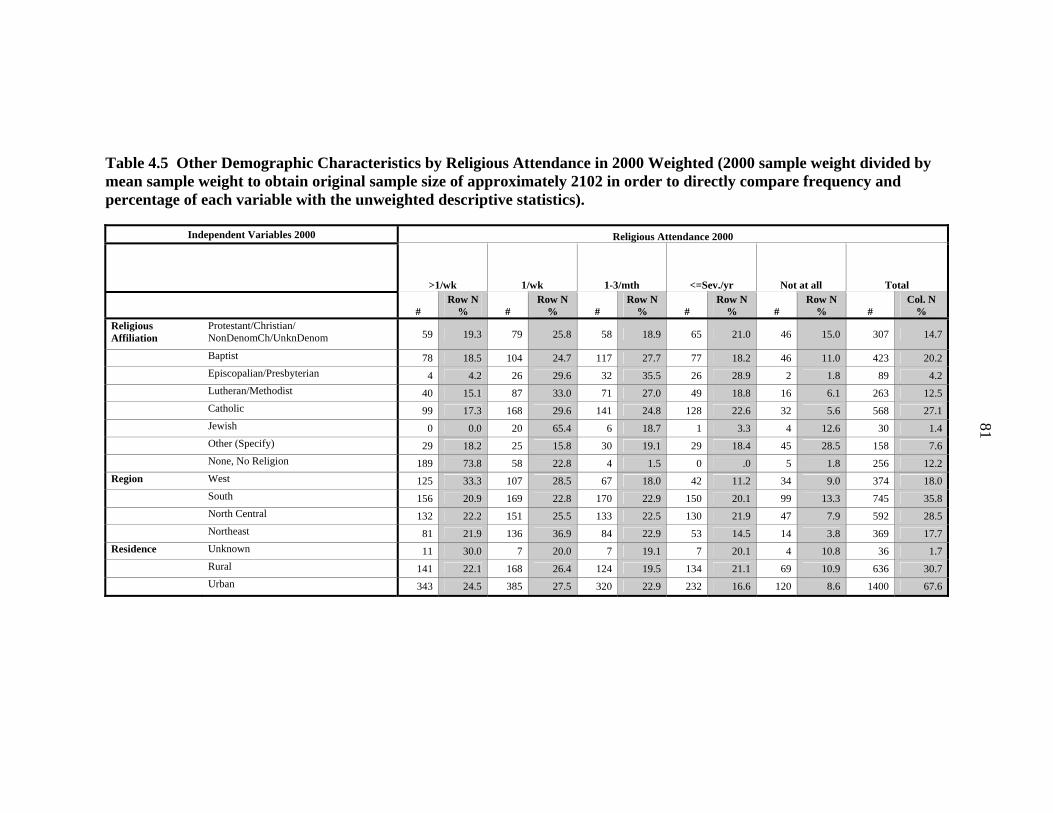
81
Table 4.5 Other Demographic Characteristics by Religious Attendance in 2000 Weighted (2000 sample weight divided by mean sample weight to obtain original sample size of approximately 2102 in order to directly compare frequency and percentage of each variable with the unweighted descriptive statistics).
Independent Variables 2000 Religious Attendance 2000
>1/wk 1/wk 1-3/mth <=Sev./yr Not at all Total
# Row N
% # Row N
% # Row N
% # Row N
% # Row N
% # Col. N
% Religious Affiliation
Protestant/Christian/ NonDenomCh/UnknDenom 59 19.3 79 25.8 58 18.9 65 21.0 46 15.0 307 14.7
Baptist 78 18.5 104 24.7 117 27.7 77 18.2 46 11.0 423 20.2 Episcopalian/Presbyterian 4 4.2 26 29.6 32 35.5 26 28.9 2 1.8 89 4.2 Lutheran/Methodist 40 15.1 87 33.0 71 27.0 49 18.8 16 6.1 263 12.5 Catholic 99 17.3 168 29.6 141 24.8 128 22.6 32 5.6 568 27.1 Jewish 0 0.0 20 65.4 6 18.7 1 3.3 4 12.6 30 1.4 Other (Specify) 29 18.2 25 15.8 30 19.1 29 18.4 45 28.5 158 7.6 None, No Religion 189 73.8 58 22.8 4 1.5 0 .0 5 1.8 256 12.2Region West 125 33.3 107 28.5 67 18.0 42 11.2 34 9.0 374 18.0 South 156 20.9 169 22.8 170 22.9 150 20.1 99 13.3 745 35.8 North Central 132 22.2 151 25.5 133 22.5 130 21.9 47 7.9 592 28.5 Northeast 81 21.9 136 36.9 84 22.9 53 14.5 14 3.8 369 17.7Residence Unknown 11 30.0 7 20.0 7 19.1 7 20.1 4 10.8 36 1.7 Rural 141 22.1 168 26.4 124 19.5 134 21.1 69 10.9 636 30.7 Urban 343 24.5 385 27.5 320 22.9 232 16.6 120 8.6 1400 67.6

82
Table 4.5 (Continued).
Independent Variables 2000 Religious Attendance 2000
>1/wk 1/wk 1-3/mth <=Sev./yr Not at all Total
# Row N
% # Row N
% # Row N
% # Row N
% # Row N
% # Col. N
% Occupation Missing 54 23.8 67 29.8 52 22.8 36 15.9 18 7.8 227 10.8 Household 7 33.7 7 32.5 5 23.3 0 .0 2 10.6 21 1.0 Blue Collar 133 23.5 149 26.3 118 20.7 102 17.9 65 11.5 567 27.1 Farmer/Armed Forces 3 16.9 4 23.3 4 23.2 4 28.0 1 8.6 15 0.7 Service/Clerical/Sales 145 24.1 168 27.9 131 21.8 113 18.8 45 7.4 602 28.7 White Collar 157 23.7 172 26.0 148 22.3 121 18.3 65 9.7 663 31.7Poverty Status Missing 89 25.2 88 24.8 64 18.1 73 20.6 40 11.2 353 16.8 Poverty 68 33.7 55 26.9 37 18.3 24 11.8 19 9.3 203 9.7 Not in Poverty
343 22.2 426 27.6 358 23.2 280 18.1 137 8.9 1543 73.5
Religious Attendance Total 500 23.8 568 27.0 459 21.9 377 17.9 196 9.3 2099 100.0
Note: The 2000 weight adjusts for loss to follow-up after the year 1979 in which the survey was administered through the year 2000. The sample 2000 weight adjusts for over-sampling of minorities, particularly Hispanics and African Americans. The weight also adjusts for two groups that were over-sampled and later dropped from the study. In 1985 an over-sample of approximately 1000 military personnel were dropped while 200 remained in the sample. In 1991 the over-sample of economically disadvantaged Caucasians was dropped from the study. The above descriptive statistics describe those individuals who were aged 40 and over in the year 2000, from a sample designed to be representative of noninstitutionalized people born between 1957 through 1964, living in the United States in 1978 (S. McClaskie, personal communication, Fall 2005).

83
Table 4.6 Demographic Characteristics by Religious Attendance in 2000 Weighted (2000 sample weight used to obtain descriptive statistics from the study sample which was designed to be representative of those age 40 and over in 2000 among the noninstitutionalized U.S. population born between 1957 and 1964).
Religious Attendance 2000
>1/wk 1/wk 1-3/mth <=Sev./yr Not at all Total Independent Sociodemographic
Control Variables 2000
# Row N % # Row N % # Row N % # Row N % # Row N % # N % Religious Affiliation Protestant/
Christian/ NonDenom./ UnknDenom
263714 19.3 351339 25.8 258196 18.9 286433 21.0 204196 15.0 1363878 14.7
Baptist 347083 18.5 463226 24.7 519444 27.7 341633 18.2 206283 11.0 1877669 20.2 Episcopalian/
Presbyterian 16629 4.2 117052 29.6 140200 35.5 114005 28.9 6954 1.8 394841 4.2
Lutheran/ Methodist 176245 15.1 384463 33.0 314040 27.0 219260 18.8 70813 6.1 1164822 12.5
Catholic 437089 17.3 745777 29.6 626022 24.8 570077 22.6 141852 5.6 2520816 27.1 Jewish 0 .0 86675 65.4 24757 18.7 4323 3.3 16728 12.6 132482 1.4 Other (Specify)
127965 18.2 110937 15.8 134442 19.1 129474 18.4 200014 28.5 702832 7.6
None, No Religion 838333 73.8 258787 22.8 17600 1.5 0 .0 20772 1.8 1135491 12.2
Region West 553809 33.3 472686 28.5 299324 18.0 186490 11.2 149002 9.0 1661310 18.0 South 691679 20.9 751933 22.8 756207 22.9 665392 20.1 438163 13.3 3303373 35.8 North Central 584252 22.2 670133 25.5 589843 22.5 575430 21.9 207692 7.9 2627350 28.5 Northeast 358349 21.9 604299 36.9 374479 22.9 236468 14.5 62136 3.8 1635731 17.7 Residence Unknown 47930 30.0 31981 20.0 30514 19.1 32151 20.1 17192 10.8 159768 1.7 Rural 623904 22.1 745125 26.4 550123 19.5 595203 21.1 308040 10.9 2822395 30.7 Urban 1520693 24.5 1708529 27.5 1420668 22.9 1029230 16.6 531760 8.6 6210880 67.6
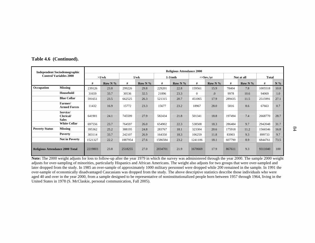
84
Table 4.6 (Continued).
Religious Attendance 2000
>1/wk 1/wk 1-3/mth <=Sev./yr Not at all Total Independent Sociodemographic
Control Variables 2000
# Row N % # Row N % # Row N % # Row N % # Row N % # N % Occupation Missing 239126 23.8 299226 29.8 229201 22.8 159561 15.9 78404 7.8 1005518 10.8 Household 31659 33.7 30536 32.5 21896 23.3 0 .0 9978 10.6 94069 1.0 Blue Collar 591651 23.5 662525 26.3 521315 20.7 451065 17.9 289435 11.5 2515991 27.1 Farmer/
Armed Forces 11432 16.9 15772 23.3 15677 23.2 18967 28.0 5816 8.6 67663 0.7
Service/ Clerical/ Sales
641901 24.1 745599 27.9 582434 21.8 501341 18.8 197494 7.4 2668770 28.7
White Collar 697556 23.7 764597 26.0 654902 22.3 538508 18.3 286484 9.7 2942048 31.7 Poverty Status Missing 395362 25.2 388195 24.8 283767 18.1 323304 20.6 175918 11.2 1566546 16.8 Poverty 303114 33.7 242107 26.9 164350 18.3 106259 11.8 83903 9.3 899733 9.7 Not in Poverty 1521327 22.2 1887954 27.6 1586584 23.2 1241106 18.1 607790 8.9 6844761 73.5
Religious Attendance 2000 Total 2219803 23.8 2518255 27.0 2034701 21.9 1670669 17.9 867611 9.3 9311040 100
Note: The 2000 weight adjusts for loss to follow-up after the year 1979 in which the survey was administered through the year 2000. The sample 2000 weight adjusts for over-sampling of minorities, particularly Hispanics and African Americans. The weight also adjusts for two groups that were over-sampled and later dropped from the study. In 1985 an over-sample of approximately 1000 military personnel were dropped while 200 remained in the sample. In 1991 the over-sample of economically disadvantaged Caucasians was dropped from the study. The above descriptive statistics describe those individuals who were aged 40 and over in the year 2000, from a sample designed to be representative of noninstitutionalized people born between 1957 through 1964, living in the United States in 1978 (S. McClaskie, personal communication, Fall 2005).

85
Dependent Variables: Health Outcome
SF-12 Physical Composite Score (PCS), Mental Composite Score (MCS) and Center
for Epidemiological Study-Depression Score (CES-D)
The dependent variables examined in this study were physical and mental health
outcomes (refer toTable 4.7, Table 4.8 and Table 4.9). The physical health score was
based on the SF-12 12-item scale on self-reported general health. Each of the 12 items
was weighted differently to obtain an overall measure of a physical health composite
score (PCS) and a separate overall measure of a mental health composite score (MCS).
For the unweighted data, the mean reported physical health score (SF-12 PCS) for the
2000 calendar year sample aged 40 to 43 was 51.92, which is above the national mean
(holding age constant) of 50, and above the national mean (for ages 35-44) of 52.2
(refer to Table 4.7). The mean reported mental health score (SF-12 MCS) for the
sample was 52.80, above the national mean (holding age constant) of 50 and above the
national mean for the age group 35-44 of 50.1 (refer to Table 4.7). For MCS, a score
of 42 or lower indicates depression (M. DeRosa, SF-36 Research Center, personal
communication, Spring 2005). Another mental health variable for depression used in
the study was the Center for Epidemiological Study Depression (CES-D) score. This
score is based on 7 items, scaled 0-3, with a possible score range of 0-21. The cut-off
point as an indicator for depression for these 7 items is a score of 6 or greater (J.
Zagorsky, the Ohio State University, personal communication, Spring 2005) The mean
CES-Depression score for this study sample was 3.5, which is below the threshold of
the depression cut-off point of 6 (refer to Table 4.7).
The summary statistics using the sample weight for the calendar year 2000 showed
slightly better physical health, mental health and depressions scores than the

86
unweighted data (refer to Table 4.7). However, the reported standard error and
deviation for the weighted summary statistics were more precise than they actually
should be because the design effect of clustering was not accounted for with the
sample weight for the calendar year 2000. Therefore, it is unclear if the reported
weighted health scores were actually slightly better compared with the unweighted
health scores.
The unweighted highest mean PCS and MCS scores and the lowest depression score
(indicating better health) were reported for those who attend religious services
“several times per year or less” (52.7 [PCS], 53.2 [MCS], 3.0 [CES-D]; refer to Table
4.8). Those who reported the lowest physical health score and highest depression score
(indicating poorer health) were the most frequent attenders, at “more than once per
week” (50.7 [PCS], 4.0 [CES-D]). Those who reported the lowest mean mental health
score (indicating poorer health) were those who attended “about once per week” (52.4
[MCS]; refer to Table 4.8).
For the weighted data as shown in Table 4.9, using the sample weight for the calendar
year 2000, the best physical health, mental health, and depression scores occurred for
those who attended infrequently in the year 2000. The worst physical health, mental
health, and depression scores occurred for those who attended the most frequently,
more than once a week (refer to Table 4.9). Note, however, that the standard errors
were more precise than they should be because the design effect of clustering was not
taken into account in the sample weight for the calendar year 2000.

87
Table 4.7 Summary Statistics for NLSY79 SF-12 Physical Health Composite (SF-12 PCS), Mental Health Composite Score (SF-12 MCS), and CES-Depression (CES-D) Scores (40 and over age group) (without controls) Unweighted and Weighted (with sample wt. 2000a).
a Weight used is 2000 sample weight, which accounts for most over-sampling of African Americans and Hispanics, and attrition from 1979 to 2000. This weight also accounts for the dropped over-samples of military personnel and economically disadvantaged Caucasians. A limitation of this sample weight is that it does not account for the design effect of clustering. This limitation produces a more precise standard error (SE) and standard deviation (SD) for the weighted summary statistics than is actually correct. The SE and SD in the table above are not correct, presenting a more precise estimate than they actually should be (CHRR 2004). b Physical Health Composite Score (PCS) is created from a weighted total score based on each of the SF-12 items. The mean score for the U.S. population is 50. c Mental Health Composite Score (MCS) is created from weighted total score based on each of the SF-12 items. The cutpoint indicating depression in the U.S. population is >=42. d Center for Epidemiological Study Depression Total Score: Summation of Total score based on 7 items. The cut-off point indicating depression is >=6 (J. Zagorsky, personal communication, Spring 2005).
Table 4.8 Dependent Variable Health (PCS, MCS and CES-Depression) 2000 Mean Scores by Religious Attendance 2000 (without controls) Unweighted.
Religious Attendance 2000
> 1/wk About 1/wk About 1-3/mth <=Sev./yr
(Infrequent) Not at all
Dependent Variable 2000 Mean (µ) SE Mean (µ) SE Mean (µ) SE Mean (µ) SE Mean (µ) SE
SF-12 PCS Scorea 50.7 0.5 52.2 0.3 52.5 0.4 52.7 0.4 51.0 0.6
SF-12 MCS Scoreb 52.6 0.4 52.4 0.4 53.1 0.4 53.2 0.4 52.7 0.6
CES-Depression Scorec 4.0 0.2 3.5 0.2 3.4 0.2 3.0 0.2 3.6 0.3 a Physical Health Composite Score (PCS) is created from a weighted total score based on each of the SF-12 items. The mean score for the U.S. population is 50. b Mental Health Composite Score (MCS) is created from weighted total score based on each of the SF-12 items. The cutpoint indicating depression in the U.S. population is >=42. c Center for Epidemiological Study Depression Total Score: Summation of Total score based on 7 items. The cut-off point indicating depression is >=6 (J. Zagorsky, personal communication, Spring 2005).
Health Variable
NLSY79 2000 (ages 40-43) Unweighted
NLSY79 2000 (ages 40-43) Weighted
(2000 sample wt)*
US population (ages 35-44)
US population (age held constant)
Mean (µ) SD SE N Mean
(µ) SD SE Mean (µ) SD Mean (µ) SD
SF-12 PCS Scoreb 51.92 8.32 0.18 9289680 52.47 7.87 .26
52.2 7.3
50.0
10.0
SF-12 MCS Scorec 52.80 8.74 0.19 9289680 52.99 8.36 .27 50.1 8.6
50.0
10.0
CES-Depression
Scored 3.50 4.44 0.10 9302718 3.17 4.18 .001

88
Table 4.9 Dependent Variable Health (PCS, MCS and CES-Depression) 2000 Mean Scores by Religious Attendance 2000 (without controls) Weighted (2000 sample weight used).a
Religious Attendance 2000
>1/wk 1/wk 1-3/mth <=Sev./yr Not at all Dependent Variable 2000
Mean SE Mean SE Mean SE Mean SE Mean SE
SF-12, PCS 2000 Scoreb 51.43 .41 52.39 .35 53.15 .33 53.62 .35 51.52 .70
SF-12, MCS 2000 Scorec 52.29 .41 52.51 .40 53.44 .38 53.83 .39 53.43 .63
CES-Depression Scored 3.91 .22 3.31 .19 2.82 .18 2.49 .19 2.99 .34a Weight used is 2000 sample weight, which accounts for most over-sampling of African Americans and Hispanics, and attrition from 1979 to 2000. This weight also accounts for the dropped over-samples of military personnel and economically disadvantaged Caucasians. A limitation of this sample weight is that it does not account for the design effect of clustering. This limitation produces a more precise standard error (SE) for the weighted summary statistics than is actually correct. The SE in the table above are not correct, presenting a more precise estimate than it actually should be (CHRR 2004). b Physical Health Composite Score (PCS) is created from a weighted total score based on each of the SF-12 items. The mean score for the U.S. population is 50. c Mental Health Composite Score (MCS) is created from weighted total score based on each of the SF-12 items. The cutpoint indicating depression in the U.S. population is >=42. d Center for Epidemiological Study Depression Total Score: Summation of Total score based on 7 items. The cut-off point indicating depression is >=6 (J. Zagorsky, personal communication, Spring 2005).
Objective I Results
Objective I.: Religious Attendance Frequency: Results of General Linear Model
Analysis
Results for Objective I.1: Simple Model: Physical Health and Religious Attendance
with controls and no interactions
Cross-sectional analysis was performed to investigate the relationship between
religious attendance and physical health, measured as an SF-12 Physical Composite
Score (PCS). Key sociodemographic variables were controlled for, including gender,
race, marital status, education, number of children, work amount, and income (refer to
Table 4.1). The variables of religious affiliation, region, residence, occupation, and

89
poverty status were included as controls in the model but were dropped because they
were not found to be significant (refer to Table 4.4).
For the simple model (in the presence of key controls, with no interactions), a U-
shaped curve for health was apparent across levels of religious attendance (refer to
Table 4.4). The lowest physical health scores occurred at the two extremes of
attendance “>1/wk” (mean [µ] score, 48.4), and “not at all” attendance (µ = 48.1),
while increasing health scores ranging from 49.2 to 49.5 occurred with more moderate
attendance, “about 1/wk,” “1-3/mth,” and infrequent attendance (measured as “less
than or equal to several times/year”). At each of the levels of religious attendance, the
mean physical health scores were slightly lower than the overall mean for the sample
of 51.9 and the U.S. population (ages 35-44) of 52.2.
As indicated in Table 4.10, better physical scores were related to the following
sociodemographic characteristics: having two or more children (B=1.0 [0.1, 1.9] CI
95%, p=0.03), working 20 or more hours per week in the past calendar year of 1999
(B=6.1 [5.2, 7.0] CI 95%, p = 0.00), and having an income in the range of mid-50
percent (>=$20,600 to <=$69,800; B=2.8 [1.8, 3.8] CI 95%, p=0.00) to top-25 percent
(>=$70,000; B=3.3 [2.0, 4.5] CI 95%, p=0.00). Hispanics were found to have lower
physical health relative to the reference group of Caucasians and others at borderline
significance (B=-0.9 [-1.9,-0.02] CI 95%, p = 0.05).

90
Not at all<=Sev./yr1-3/mth1/wk>1/wk
Religious Attendance 2000
49.50
49.20
48.90
48.60
48.30
48.00
Est
imat
ed M
argi
nal M
eans
Estimated Marginal Means of Physical Health Composite Score (SF-12, PCS)2000
Figure 4.1 Obj. I. Simple Model. Physical Health Composite Score (SF-12 PCS) in 2000 by Religious Attendance in 2000 controlling key sociodemographic variables in 2000 (as listed in Table 4.1: gender, race/ethnicity, marital status, education, children living in the household, work amount in 1999 and net family income in 1999).
In a preliminary analysis, religious affiliation was investigated as an independent
variable in relation to the dependent health variables, controlling for key
sociodemographic variables listed in Table 4.1. Due to low cell count in some of the
religious affiliations, however, the variable was dropped from the model. The
preliminary analysis found that religious affiliation was somewhat significantly related
to each of the health variables in the simple model. Those who reported affiliation
with the Jewish faith had the highest health scores, controlling for sociodemographic
variables (listed in Table 4.1).

91
Table 4.10 Obj. I. Parameter Estimates of Simple Model (no Interactions) for Dependent Variables in 2000 of Physical Health Composite Score (SF-12 PCS), Mental Health Composite Score (SF-12 MCS) and CES-Depression Score (CES-D) by Religious Attendance in 2000 (controlling for sociodemographic variables in 2000 of gender, race/ethnicity, marital status, education, number of children living in the household, work amount in 1999, net family income in 1999, residence and region).
Independent Control Variables
2000
Physical Health Composite Score (SF-12 PCS 2000)
Mental Health Composite Score (SF-12 MCS 2000)
CESD-Depression Score (CES-D 2000)
Parameter B Sig. CI 95% B Sig. CI 95% B Sig. CI 95
%
Intercept 43.4 .00 40.9 45.8 48.8 .00 46.0 51.6 5.5 .00 4.1 6.9
Rel. Attend. >1/wk (RA) .2 .73 -1.1 1.5 .1 .90 -1.3 1.5 .4 .26 -.3 1.1
RA 1/wk 1.1 .09 -.2 2.3 -.4 .52 -1.8 .9 .2 .58 -.5 .9
RA 1-3x/mth 1.1 .07 -.1 2.4 .1 .88 -1.3 1.5 -.1 .86 -.7 .6 RA <=Sev.x/yr (Infreq.) 1.4 .04 .1 2.6 .2 .80 -1.2 1.6 -.2 .55 -.9 .5
RA Not at all (No) 0(a) . . . 0(a) . . . 0(a) . . .
Female -.5 .14 -1.2 .1 -2.0 .00 -2.7 -1.2 .9 .00 .6 1.3
Male 0(a) . . . 0(a) . . . 0(a) . . .
Hispanic -.9 .05 -1.9 -0.02 .4 .42 -.6 1.5 .3 .21 -.2 .9
African American -.4 .30 -1.3 .4 .2 .61 -.7 1.2 .5 .02 .1 1.0 Caucasian and Others 0(a) . . . 0(a) . . . 0(a) . . .
Widow/Separated -1.0 .20 -2.5 .5 -1.2 .16 -2.9 .5 .4 .37 -.4 1.2
Divorced -.7 .24 -1.9 .5 -1.1 .10 -2.4 .2 1.0 .00 .4 1.6
Married -.1 .86 -1.2 1.0 .0 .99 -1.2 1.2 -.2 .54 -.8 .4
Never Married 0(a) . . . 0(a) . . . 0(a) . . . > High School (HS) 1.5 .13 -.5 3.5 1.0 .39 -1.2 3.2 -.6 .24 -1.7 .4
High School .5 .60 -1.4 2.4 .3 .82 -1.9 2.4 .1 .90 -1.0 1.1
< High School 0(a) . . . 0(a) . . . 0(a) . . .
>=2 Children 1.0 .03 .1 1.9 .4 .45 -.6 1.4 -.1 .59 -.6 .3
1 Child -.4 .47 -1.4 .7 -.3 .56 -1.5 .8 .2 .40 -.3 .8
No Children 0(a) . . . 0(a) . . . 0(a) . . . Work Amt. in 1999 >20 hrs/wk (FT)
6.1 .00 5.2 7.0 3.6 .00 2.6 4.7 -2.0 .00 -2.5 -1.5
Work Amt. in 1999 0-20 hrs/wk (PT)
0(a) . . . 0(a) . . . 0(a) . . .
Income in 1999 Missing 2.1 .00 .9 3.2 .6 .34 -.6 1.9 -1.0 .00 -1.7 -.4
Income in 1999 Top 25% 3.3 .00 2.0 4.5 2.4 .00 1.0 3.8 -2.2 .00 -2.9 -1.5
Income in 1999 Mid 50% 2.8 .00 1.8 3.8 1.4 .01 .3 2.5 -1.8 .00 -2.4 -1.3
Income in 1999 Lowest 25% 0(a) . . . 0(a) . . . 0(a) . . .

92
Table 4.10 (Continued).
Independent Control Variables
2000
Physical Health Composite Score (SF-12 PCS 2000)
Mental Health Composite Score (SF-12 MCS 2000)
CESD-Depression Score (CES-D 2000)
Parameter B Sig. CI 95% B Sig. CI 95% B Sig. CI 95
% Residence: Unknown 5.0 .00 2.3 7.7
Rural .8 .08 -.1 1.7
Urban 0(a) . . .
Region: West .4 .21 -.2 1.0
South .7 .01 .1 1.2
North Central .4 .14 -.1 1.0
Northeast 0(a) . . . Adj. R Square 0.153 0.068 0.146 Corrected Model df
18 20
21
Error df 2055 2022 2036 Total df 2074 2043 2058 F 21.8 8.5 17.7 Sig. 0.00 0.00 0.00
Interactions in Models with Outcome Variable of Physical Health Composite Score
(PCS): Interaction Models, Attendance with Education, Work, and Income
In order to better understand how key sociodemographic variables influenced the
relationship between religious attendance and health, interactions were tested with
each key sociodemographic variable and religious attendance listed in Table A.1 and
Table A.2.
The three main variables interacting with religious attendance were education, work
amount, and income. The main result found was that those who reported no attendance
and had either low education level (0-8 grades), low work hours (0-20 hrs/wk), or low
income (low 25 % [<=$20,516]), reported lower health scores than those who reported
attending more frequently.

93
Two-Way Interaction Model: Attendance*Education
The interaction between attendance and education was significant. For the highest
level of attendance (“>1/wk”), those with less than a high school education had a
slightly higher mean physical health score than those with some high school
education. Moreover, comparing these two education groups at the lowest level of
attendance (“not at all”), the physical health score for those with less than a high
school education was dramatically lower than it was for those with some high school
education (B=-8.7 [-15.7,-1.8] CI 95%, p=0.01) or some college/graduate school
education (B=-9.2 [-16.2, -2.3] CE 95%, p = 0.01; refer to Figure A.1 and Table A.2).
For those with less than a high school education (and across all education levels), the
highest mean health scores were reported at moderate attendance (“1-3/mth”; refer to
Figure A.1). This indicates that the less-educated may benefit more from attending
religious services than those with more years of education.
Two-Way Interaction Model: Attendance*Work
For the model with one interaction of attendance with work amount, all levels of
attendance with work amount were significant. Among those who report working “<
20 hrs/wk” (in the past calendar year, 1999), religious attendance frequency was
associated with a curvilinear result in health scores. Mean health scores increased
slightly as attendance became less frequent, but at no attendance, the mean health
score dropped sharply. The highest health score among those working “< 20 hrs/wk”
was infrequent attendance, and the lowest health score was reported among those who
attend “not at all” (refer to Figure A.2 and Table A.2). For those who reported
working “>20 hrs/wk,” frequency of attendance made little difference in the physical
health score, but with physical health scores that were much higher overall compared
with those of people who work “<20 hrs/wk.” This indicates that those who work less
benefit more from attending religious services than those who work more.

94
Two-Way Interaction Model: Attendance*Income
For the model with the interaction of attendance with income, those who reported the
lowest 25 percent income level (<=$20,516) had lower physical health scores with less
religious attendance, particularly when attendance was reported as “not at all,”
compared with that of those with higher incomes (mid-50% to top 25%, for which
frequency of religious attendance had little association with reported physical health
score; refer to Table A.2 and Figure A.3). For those with the lowest 25 percent
income, the highest health score occurred for those who reported attending “>1/wk,”
with lower health score as attendance decreased. For those with higher incomes (mid-
50 to top 25%), the best physical health scores occurred at moderate attendance (“1-
3/mth” to “<=several/yr.”), with the lowest scores at “not at all.” This indicates that
those with low income benefit more from attending more frequently than those with
higher income.
Multiple Two-Way Interaction Model: Attendance*Education, Attendance*Work and
Attendance*Income
In order to further understand how the two-way interactions interacted with each other,
or how two or more sociodemographic variables may each have affected the way
religious attendance influences health, multiple two-way interaction models were
analyzed (refer to Figure A.4, Figure A.5, and Figure A.6).
The model with three two-way interactions present (attendance*education,
attendance*work, and attendance*income) showed trends that were similar to those
obtained with each of the models with one interaction. For those with lowest education
“< high school,” low work “<20 hrs/wk,” and low income “$<20,600,” mean physical
health scores each showed a dramatic decrease in reported health score values at
attendance level “not at all” (refer to Figure A.4, Figure A.5, and Figure A.6). Those

95
with higher education, work amount, and income showed random variability with no
trend across categories, and no significant difference across each level of attendance
(but with higher health scores overall compared with those for the low education, low
work amount, and low income groups). This indicates that those with low SES benefit
more from some attendance than no attendance.
Two Three-Way Interaction Model: (Attendance*Income*Work) and
(Attendance*Income*Education)
A model with the two three-way interactions (attendance*income*work and
attendance*income*education) was also found to be significant (refer to ANOVA
Table A.1). Overall, those with low-to-mid income (“lowest 25%” to “mid 50%”) and
low work time “<20 hrs/wk,” reported the lowest physical health scores compared
with those who reported the highest income, “top 25%,” and more work time, “>20
hrs/wk,” across attendance levels, particularly at no attendance.
For work amount of “>20hrs/wk” for the mid 50 percent and top 25 percent income
levels, mean PCS scores were higher across religious attendance levels compared with
the lowest 25 percent income, particularly at the no attendance level. However, at
attendance of “1/wk” the top 25 percent income had the lowest PCS mean score of all
income levels and attendance levels.
At the highest education level, “>high school,” those with the lowest 25 percent
income had the lowest health scores compared with those with the highest income (top
25%) at religious attendance “>1/wk” relative to reported attendance level “not at all.”

96
Results for Objective I.2 Mental Health (SF-12 MCS) Association with Religious
Attendance Frequency
Simple Model: Mental Health and Religious Attendance (with controls and no
interactions)
Cross-sectional analysis was performed on the relationship between religious
attendance and mental health (measured as SF-12 Mental Composite Score [MCS]).
Key sociodemographic variables were controlled for, including gender, race, marital
status, education, number of children, work amount, income, and residence (rural vs.
urban). The following variables—religious affiliation, region, occupation, and poverty
status—were included as controls in a preliminary analysis but were dropped in the
final model because they were not found to be significant. For the simple model (in
the presence of controls, with no interactions), religious attendance was not
significantly related to mental health (refer to Table 4.10). The mean scores for mental
health were consistent (52.7 to 52.9) across levels of religious attendance, except for
attendance “1/wk,” with a lower mental health score (µ = 52.3; refer Figure 4.2).
These scores were higher than the national average (ages 35-44) at 50.1. As indicated
in Table 4.10, females had a lower mean mental health score (thus poorer mental
health) relative to males (B=-2.0 [-2.7, -1.2] CI 95%, p = 0.00). Those with higher
mean mental health scores (thus better mental health) were those working >20 hrs/wk
(B= 3.6 [2.6, 4.7] CI 95%, p=0.00), and those with incomes at levels of mid-50
percent (B=1.4 [0.3, 2.5] CI 95%, p=0.01) to top 25 percent (B=2.4 [1.0, 3.8] CI 95%,
p=0.00). Place of residence was significant only for those whose residence was
reported as “unknown” (B=5.0 [2.3, 7.7] CI 95%, p=0.00). Place of residence was not
significant for models with the dependent variable of physical health (PCS) or CES-
Depression.

97
Not at all<=Sev./yr1-3/mth1/wk>1/wk
Religious Attendance 2000
52.90
52.80
52.70
52.60
52.50
52.40
52.30
52.20
Est
imat
ed M
argi
nal M
eans
Estimated Marginal Means of Mental Health Composite Score (SF-12, MCS)2000
Figure 4.2 Obj. I. Simple Model. Mental Health Composite Score (SF-12 MCS) in 2000 by Religious Attendance in 2000 (controlling for socio-demographic variables in 2000 of gender, race/ethnicity, marital status, education, children living in household, work amount in 1999, net family income in 1999, residence and region).
Interactions in Models with Outcome Variable of Mental Health Composite Score
(MCS) Model: Interaction Models, Attendance with Race/Ethnicity and Education
Two-Way Interaction Model: Attendance*Race/Ethnicity
The interaction of attendance with race/ethnicity was found to be significant. The
significant interaction occurred between African Americans and higher frequencies of
religious attendance of more than once per week to once per month (refer to Table
A.3).. African Americans who attended the most frequently, more than once per week,
had the highest reported scores for mental health (within their ethnic/racial group and

98
among other ethnic/racial groups). African Americans had generally lower mental
health scores with decreasing attendance, with the lowest health score at the
attendance level of “not at all.” The ethnic/racial group of Caucasians and others
showed the opposite trend, revealing better mental health scores with decreasing
attendance (refer to Table A.3 and Figure A.7).
In an attempt to better understand the differences in mental health outcomes among
the three race/ethnicities, regression models were run separately for each race and
ethnicity. This analysis is described at the end of Chapter 4 and Objective 1.4, and in
Table 4.11, Figure 4.4, Figure 4.5, and Figure 4.6.
Two-Way Interaction Model: Attendance*Education
The interaction of education level with attendance significantly influenced mental
health scores. For those who attended religious services once per week, individuals
with less than a high school education had much lower mental health scores than those
with some high school education or more; however, this low education group had
higher mental health scores at attendance levels “>1/wk” and “1-3/mth” compared
with the other educational levels (refer to Table A.3).
Multiple Two-Way Interaction Model: Attendance*Race/Ethnicity and
Attendance*Education
A similar interaction effect of race and attendance was apparent in the model that
included the presence of the interaction of attendance with education. The lowest
mental health score for all ethnicities was at attendance of once per week (refer to
Figure A.9). The same interaction trend for attendance with education was also present
in the model that included the additional interaction of attendance with race (refer to
Figure A.10).

99
Three-Way Interaction Model: Race/Ethnicity*Education*Attendance
A three-way interaction of race, education, and attendance was found to be significant
at the level of some high school and some college/graduate school education, and for
the racial group Hispanics at the level of attendance of once per week relative to no
attendance. The general trend for the education level of some high school was that
Hispanics as well as African Americans reported better mental health scores with
more frequent attendance, whereas Caucasians and others showed the opposite trend.
For the education level of some college or more, comparing the scores of Caucasians
and others with those of Hispanics and African Americans, the mental health scores of
the latter two groups were higher at the most frequent attendance level of more than
once per week, decreasing at once per week, then increasing in score as attendance
levels decreased from moderate to no attendance. For the most frequent attendance
level, more than once per week, Hispanics and African Americans reported much
better mental health relative to Caucasians and others. Overall, it appeared that
African Americans and Hispanics had better mental health with high attendance of
more than once per week compared with Caucasians. Note, however, that health
scores fluctuated across attendance levels by ethnicity and education. The interactions
were explored and are discussed here, but the tables and figures are not included
because of the fluctuation in health scores and a lack of consistent and obvious
patterns for these interactions.
Results for Objective I.3 Depression (CES-D) Association with Religious Attendance
Frequency
Simple Model: Depression and Religious Attendance (with controls and no
interactions)

100
Cross sectional analysis was performed on the relationship between religious
attendance and CES-Depression scores. The following sociodemographic variables
were controlled for: gender, race, marital status, education, number of children, work
amount, income, and region of residence within the United States. The following
variables—religious affiliation, occupation, residence, and poverty status—were
included as controls in a preliminary model but were dropped because they were not
found to be significant (refer to Table 4.4).
For the simple model (in the presence of controls, with no interactions), frequency of
religious attendance was not significantly related to the depression score (refer to
Table 4.10). A decreasing curve-shaped trend occurred across levels of religious
attendance with an increase at the no attendance level (refer to Figure 4.3). The
highest mean depression score occurred at the highest level of attendance, more than
once per week (µ = 4.9; a score of 6 or more was an indicator for depression). Lower
scores for depression occurred with low attendance levels (“1/wk” to infrequent, µ =
4.7 to 4.3). A very slight increase in the mean depression score occurred at the no
attendance level, increasing from the infrequent attendance level. (µ = 4.5; refer to
Figure 4.3). The sociodemographic characteristics that were related to higher mean
depression scores were being female (B=0.9 (0.6,1.3) CI 95%, p=0.00), African
American (B=0.5 (0.1, 1.0) CI 95%, p=0.02), divorced (B=1.0 (0.4,1.6) CI 95%,
p=0.00), and living in the region of the South (B=0.7 (0.1,1.2) CI 95%, p=0.01) (refer
to Table 4.10). The variable for region of residence in the U.S. was not significant for
models with the dependent variable of physical (PCS) or mental health (MCS).

101
Not at all<=Sev./yr1-3/mth1/wk>1/wk
Religious Attendance 2000
5.00
4.90
4.80
4.70
4.60
4.50
4.40
4.30
Est
imat
ed M
argi
nal M
eans
Estimated Marginal Means of CES-Depression Score
Figure 4.3 Obj. I. Simple Model. CES-Depression in 2000 by Religious Attendance in 2000 (controlling for sociodemographic variables in 2000 of gender, race/ethnicity, marital status, education, children living in household, work amount in 1999, net family income in 1999, residence and region).
Having a lower mean depression score was related to working less than twenty hours
per week (B=-2.0 [-2.5,-1.5] CI 95%, p=0.00), and having an income at the level of
top 25 percent (B=-2.2 [-2.9,-1.5] CI 95%, p=0.00) to mid 50 percent(B=-1.8 [-2.4,-
1.3] CI 95%, p=0.00; refer to Table 4.10).

102
Interactions in Models with the Outcome Variable of CES-Depression Model:
Interaction Models, Attendance with Race/Ethnicity and Marital Status
Two-Way Interaction Model: Attendance*Race/Ethnicity
The interaction of race/ethnicity with attendance was found to be significant for the
cross-sectional model of the dependent variable of CES-Depression (refer to Table
A.4). The significant interaction occurred between African Americans and higher
frequencies of religious attendance from more than once per week to once per month.
African Americans who attended more frequently scored lower for depression than
African Americans who did not attend (refer to Figure A.11). However, the
ethnic/racial group Caucasians and others reported higher scores for depression with
increased frequency of attendance compared with the scores of African Americans.
This same trend occurred with the mental health composite score (MCS) outcome as
well.
In an attempt to better understand the differences in depression outcomes among the
three race/ethnicities, regression models were run separately for each race and
ethnicity (refer to Table 4.12 and Figure 4.7, Figure 4.8 and Figure 4.9). This is further
explained toward the end of Chapter 4, in Objective 1.4.
Two-Way Interaction Model: Attendance*Marital Status
There was an interaction at the most frequent attendance level of more than once per
week and the marital status of widowed or separated. Widowed or separated who
attended more than once per week had the lowest depression score for any of the
marital status groups and the highest depression score if they did not attend at all (refer
to Table A.4 and Figure A.12). In contrast, married who attended more than once per
week had higher depression scores than those who never attended.

103
Three-Way Interaction Model: Attendance* Race/Ethnicity*Marital Status
A three-way interaction of race/ethnicity, marital status, and attendance was found to
be significant mainly for the race of Hispanics and marital status of
widowed/separated at moderate attendance level (1-3/mth), although there was a
problem with low numbers among the sub-categories, so the results may not be
reliable. Widowed or separated Hispanics and African Americans who attended
moderately, once to three times per month, scored lower for depression than those who
did not attend. Likewise, divorced Hispanics who attended moderately scored low for
depression compared with those who did not attend at all. The opposite trend was
present for Caucasians and others who were widowed/separated and attended
moderately (as this group scored high for depression compared with the no attendance
group).
Objective 1.4 Simple Regression Model of Mental Health Composite Score (MCS) and
CES-Depression (CES-D) Run Separately by Race/Ethnicity and Gender
In the analysis of the simple and full regression models for mental health (refer to
Table A.3) and depression (refer to Table A.4), females were found to have
significantly poorer mental health and to be more depressed than males. In addition,
the interaction of race/ethnicity and religious attendance was found to be significantly
related to mental health and depression. African Americans who attended religious
services more frequently reported better mental health scores (refer to Table A.3 and
Figure A.7) and lower depression scores (Table A.4 and Figure A.11) than African
Americans who did not attend at all, while the reverse trend occurred for Caucasians
and all others. Separate regression models for each gender and each race/ethnicity
were performed to better study the differences between men and women and African
Americans and Caucasians in mental health and depression scores relative to religious
attendance levels.

104
It is useful to run separate regression models for each level of gender and
race/ethnicity , rather than to force multiple interactions in one overall model (which
becomes difficult to interpret), because this procedure allows comparisons among the
regression models for each separate gender and for each separate race/ethnicity,
producing the effect of simultaneous interactions of gender (or race/ethnicity) with all
the other independent control variables in the model. Using the statistical program
SPSS version 13.0, a split file was created to run separate regression models for each
gender, male and female. Another split file was created to run separate regression
models for each of the three main race/ethnicity groups present in the dataset: (1)
Hispanic, (2) African American, and (3) Caucasian and all others.
Simple Regression Model of Mental Health Composite Score (MCS) by Gender
The separate regression models by gender for males and females were compared for
each health outcome. The differences were not worthy of special note. The religious
attendance variable was not significant for the separate regression models by males
and females for the mental health or depression outcome variables. Separate
regression models by gender were also run for the outcome variable of physical health.
Some of the religious attendance levels were found to be significant in the model run
only for females in the physical health model. The female-only model revealed a U-
shaped trend similar to the overall physical health model, but with slightly lower
scores (with better health scores at attendance levels of once per week to infrequent
and lower health scores at the two extremes of attendance, greater than once per week
and not at all) (refer to Table 4.10 and Figure 4.1). None of the religious attendance
levels were significant in the physical health model run only for males (although the
physical health scores for the male-only model were higher than for the overall model
and for the female-only model, with a U-shaped curve similar to the overall model).

105
Simple Regression Models of Mental Health Composite Score (MCS) for African
Americans compared to Caucasians and all others
The separate regression models by race/ethnicity produced interesting significant
relationships with the dependent health outcome variables of mental health and
depression, but not for the outcome variable of physical health. The details of the
results are described in the following paragraphs.
None of the parameter estimates for any of the levels of the independent variable of
religious attendance were significantly associated with the dependent variable of
mental health in the overall simple model (before separating by race/ethnicity) (refer
to Table 4.10). However, some parameter estimates for the levels of religious
attendance were significantly related to mental health in the regression models run
separately for African American and Caucasians and all others (refer to Table 4.11).
None of the religious attendance levels were significant in the regression model run
separately for Hispanics (refer to Table 4.11).
There was a striking contrast in mental health composite scores by religious
attendance levels between the two race/ethnicities of African Americans and
Caucasians. African Americans who attended more frequently, particularly at more
than once per week, reported higher (better) mental health scores than African
Americans who did not attend at all, almost three points higher in an average mental
health score (B=2.9, p =0.04; refer to Table 4.11 and Figure 4.5). Hispanics showed a
trend similar to African Americans, although the trend was not significant (refer to
Table 4.11 and Figure 4.4).

106
The reverse trend in mental health scores by religious attendance occurred for
Caucasians and all others compared to African Americans. Caucasians and all others
who reported more frequent attendance reported lower (poorer) mental health scores,
in an obvious linear trend (refer to Table 4.11 and Figure 4.6). Caucasians and all
others who attended more than once per week reported an average mental health
composite score two points lower than those who never attended (B=-2.0, p=0.04;
refer to Table 4.11, Figure 4.6).
The amount of variance in mental health scores which each model explained was the
highest in the model for African Americans (adjusted R2 = 0.106; refer to Table 4.11).
This explained variance in mental health scores for the model of African Americans
was almost double compared to the variance in mental health scores explained by the
overall model (adjusted R2 = 0.068; refer to Table 4.10) and the variance in mental
health scores explained by the model for Caucasians and others (adjusted R2 = 0.048;
refer to Table 4.11).
The other sociodemographic variables that were significantly related to mental health
for African Americans were gender, work amount, and residence (refer to Table 4.11).
African American females reported a lower average mental health score than African
American males by 3.5 points. In contrast, Caucasians and all other females reported
only 1.4 points lower in average mental health scores compared to Caucasian and all
other males (refer to Table 4.11).
African Americans who reported working 20 hours or more per week also reported
higher average mental health scores by 5.4 points compared to those who worked less

107
than 20 hours per week. Caucasians and all others who worked 20 or more hours per
week only reported average mental health scores 1.5 points higher compared to those
who worked less than 20 hours per week (refer to Table 4.11).
African Americans who lived in an urban environment reported 6.2 points lower in
average mental health scores compared to those whose residence was unknown.
Caucasians and all others who lived in an urban residence reported only 3.3 points
lower in average mental health scores compared to those whose residence was
unknown, and only one point lower in average mental health scores for those whose
residence was rural compared to an unknown residence (refer to Table 4.11).
Interestingly, the sociodemographic variables of education, number of children living
in the household, and income were not significantly related to mental health composite
scores for African Americans; however, these sociodemographic variables were
significantly related to mental health composite scores for Caucasians and all others
(refer to Table 4.11).
Caucasians and all others who reported some education beyond high school reported
average mental health scores 3.6 points higher than those with no high school
education (refer to Table 4.11).
Caucasians and all others who reported living in the same household with one child
reported 1.5 lower average mental health scores than those living with no children.
Caucasians living with two or more children were not significantly different from
those living with no children (refer to Table 4.11).

108
Caucasians who reported income in the top 25th to mid 50th percentiles reported
average mental health scores of 1.8 and 1.5 points higher, respectively, compared to
those who reported income in the lowest 25th percentile (refer to Table 4.11).
The marital status of being divorced was borderline significantly related to slightly
lower mental health scores (B=-1.1, p=0.10) compared to the unmarried in the overall
model (refer to Table 4.10), but not in any of the separate models run for each
race/ethnicity (refer to Table 4.11).
It should also be pointed out that because the observed relationship between religious
attendance and mental health and depression scores is cross-sectional, during the year
2000, attempts to explain causality can not be determined. For example, it is unclear
whether those Caucasians who attend more frequently do so in order to cope with pre-
existing poorer mental health and depression. Perhaps with no attendance, these
frequent attenders with poor mental health and depression would have even worse
mental health and depression. In an attempt to address the issue of causality, the
effects of religious attendance in young adulthood (during the year 1982) on mid-
adulthood mental health and depression as well as physical health were examined
(during the year 2000), controlling for baseline health status in 1981 and other
sociodemographic factors (during the years 1982 and 1998), as discussed in Chapter 5.

109
Table 4.11 Obj. I. Parameter Estimates of Simple Models of Dependent Variable Mental Health Composite Score (SF-12 MCS) in 2000 run separately by each Race/Ethnicity (Hispanics, African Americans and Caucasians and all others; controlling for sociodemographic variables in 2000 of gender, race/ethnicity, marital status, education, number of children living in the household, work amount in 1999, net family income in 1999, and residence).
Hispanics MCS African Americans MCS Caucasians and all others MCS Independ. Var. in 2000 Parameter B Sig. CI 95% B Sig. CI
95% B Sig. CI
95%
Intercept 45.9 .00 40.6 51.2 48.0 .00 42.6 53.5 48.7 .00 44.1 53.
2 Rel. Attend. >1/wk (RA) 1.1 .59 -2.8 4.9 2.9 .04 .1 5.8 -2.0 .04 -3.9 -.1
RA 1/wk -.1 .93 -3.6 3.3 .7 .55 -1.7 3.2 -1.7 .08 -3.5 .2
RA 1-3x/mth -.2 .92 -3.8 3.4 1.6 .19 -.8 4.0 -1.1 .29 -3.0 .9 RA <=Sev.x/yr (Infreq.) -.6 .74 -4.2 3.0 1.3 .31 -1.2 3.9 -.5 .62 -2.4 1.5
RA Not at all (No) 0(a) . . . 0(a) . . . 0(a) . . .
Female -1.2 .22 -3.1 .7 -3.5 .00 -5.1 -1.9 -1.4 .00 -2.4 -.4
Male 0(a) . . . 0(a) . . . 0(a) . . .
Widow/Separated 2.0 .35 -2.2 6.1 -2.6 .04 -5.0 -.1 1.1 .49 -2.0 4.2
Divorced .0 .99 -3.5 3.4 -1.0 .36 -3.1 1.1 -.8 .41 -2.8 1.1
Married .9 .55 -2.1 3.9 -.9 .38 -3.0 1.2 1.0 .29 -.9 2.8
Never Married 0(a) . . . 0(a) . . . 0(a) . . . > High School (HS) .5 .79 -3.1 4.0 .9 .73 -4.1 5.8 3.6 .07 -.3 7.4
High School -1.3 .44 -4.7 2.1 .5 .85 -4.4 5.3 2.8 .15 -1.0 6.7
< High School 0(a) . . . 0(a) . . . 0(a) . . .
>=2 Children .1 .92 -2.4 2.7 .8 .41 -1.1 2.7 .1 .88 -1.2 1.4
1 Child 1.4 .36 -1.6 4.3 .3 .78 -1.8 2.4 -1.5 .05 -3.0 .0
No Children 0(a) . . . 0(a) . . . 0(a) . . . Work>20 hrs/wk (FT) 6.7 .00 4.2 9.3 5.4 .00 3.4 7.4 1.5 .03 .1 2.9
0-20 hrs/wk (PT) 0(a) . . . 0(a) . . . 0(a) . . .
Income Missing 1.6 .30 -1.4 4.7 -.5 .66 -2.6 1.6 .4 .66 -1.4 2.3
Income Top 25% 2.5 .17 -1.1 6.1 2.1 .18 -1.0 5.1 1.8 .05 .0 3.6
Income Mid 50% 1.6 .26 -1.2 4.3 .2 .83 -1.8 2.3 1.5 .07 -.1 3.0 Income Lowest 25% 0(a) . . . 0(a) . . . 0(a) . . .
Residence: Unknown 5.5 .14 -1.9 12.8 6.2 .01 1.6 10.
8 3.3 .09 -.5 7.1
Rural .4 .76 -2.2 3.1 .0 .99 -2.0 2.1 1.0 .06 .0 2.0
Urban 0(a) . . . 0(a) . . . 0(a) . . . Adj. R Square 0.097 0.106 0.048 Corrected Model df 18 18 18
Error df 356 606 1024 Total df 375 625 1043 F 3.2 5.1 3.9 Sig. 0.00 0.00 0.00

110
Not at all<=Sev./yr1-3/mth1/wk>1/wk
Religious Attendance 2000
54.20
54.00
53.80
53.60
53.40
53.20
53.00
52.80
52.60
52.40
Est
imat
ed M
argi
nal M
eans
Race/Ethnicity: Hispanic
Estimated Marginal Means of Mental Health Composite Score(SF-12, MCS) 2000
Figure 4.4 Obj. I. Simple Model for Hispanics: Mental Health Composite Score (SF-12 MCS) in 2000 by Religious Attendance in 2000 (controlling for socio-demographic variables in 2000 of gender, marital status, education, children living in household, work amount in 1999, net family income in 1999, and residence.

111
Figure 4.5 Obj. I. Simple Model for African Americans: Mental Health Composite Score (SF-12 MCS) in 2000 by Religious Attendance in 2000 (controlling for sociodemographic variables in 2000 of gender, marital status, education, children living in household, work amount in 1999, net family income in 1999, and residence).
Not at all <=Sev./yr1-3/mth1/wk>1/wk Religious Attendance 2000
54.00
53.00
52.00
51.00
Race/Ethnicity: African American
Estimated Marginal Means of Mental Health Composite Score(SF-12, MCS) 2000

112
Figure 4.6 Obj. I. Simple Model for Caucasians and all others: Mental Health Composite Score (SF-12 MCS) in 2000 by Religious Attendance in 2000 (controlling for gender, marital status, education, children living in household, work amount in 1999, net family income in 1999, and residence).
Not at all <=Sev./yr1-3/mth1/wk>1/wk Religious Attendance 2000
53.00
52.50
52.00
51.50
51.00
Race/Ethnicity: Caucasians and all others
Estimated Marginal Means of Mental Health Composite Score (SF-12, MCS) 2000

113
Simple Regression Models of CES-Depression (CES-D) for African Americans
compared to Caucasians and all others
None of the religious attendance levels were significantly related to depression scores
in the simple overall model (refer to Table 4.10). However, when the same simple
model was run separately for each race/ethnicity, particularly for African Americans
and Caucasians and all others, some of the religious attendance levels became
significantly related to the outcome variable of depression (as was the case described
previously for the outcome variable of mental health; compare Table 4.11 to Table
4.12). None of the religious attendance levels were significantly related to depression
in the regression model run separately for Hispanics (refer to Table 4.12; Figure 4.7).
Therefore, the two separate models for African Americans and Caucasians and all
others were compared, as described in the following paragraphs.
African Americans who reported attending moderately often, about one to three times
per month, reported being less depressed (with lower average depression scores of
-1.2) compared to those who reported never attending (refer to Table 4.12 and Figure
4.8). In contrast, Caucasians and all others who reported attending frequently, at more
than once per week or about once per week, reported higher (poorer) average
depression score of 1.2 to 0.8 points, respectively, compared to those who reported
never attending (refer to Table 4.12 and Figure 4.9).
The amount of variance in depression scores was similar for the overall model
(adjusted (adjusted R2 = 0.146; refer to Table 4.10), as well as for each model for the
three separate race/ethnicities, Hispanics, African Americans, Caucasians and all
others, with respective adjusted R squares of 0.160, 0.132, and 0.131 (refer to Table
4.12).

114
The other sociodemographic variables which were significantly related to depression
for African Americans were gender, marital status, work amount, income, and region
in the United States the respondent reported living in (refer to Table 4.12). The overall
model (refer to Table 4.10) as well as the Caucasian and all others model (refer to
Table 4.12), reported similar significant sociodemographic variables related to
depression, with only slight differences from the model for African Americans.
African American females reported a higher (poorer) average depression score
compared to African American males by 1.5 points. In contrast, Caucasian and all
other females reported only a 0.7 point higher (poorer) average depression score
compared to Caucasian and all other males (refer to Table 4.12).
African Americans whose marital status was reported as divorced had a 0.9 higher
(poorer) average depression score compared to African Americans who reported never
being married (similar results were observed in the overall model; refer to Table 4.10).
Divorce was not significantly related to depression in the model for Caucasians and all
others (refer to Table 4.12).
African Americans who reported working 20 hours or more per week also reported a
lower (better) average depression score by -2.2 points compared to those who worked
less than 20 hours per week. Caucasians and all others who worked 20 or more hours
per week reported average depression scores only -1.3 points lower compared to those
who worked less than 20 hours per week. African Americans who reported income in
the top 25th to mid-50th percentiles reported lower average depression scores of -2.2
and -1.5, respectively. Similar results for income and depression were found for the

115
model with Caucasians (refer to Table 4.12) as well as the overall model (refer to
Table 4.10).
African- Americans who reported living in the South reported a one-point higher
(poorer) average depression score compared to those who reported living in the
Northeast, while Caucasians and all others who reported living in the West, South, and
North Central regions of the United States reported slightly higher average depression
scores compared to those living in the Northeast (B=0.8, 0.7, and 0.7 respectively,
p<=0.05; refer to Table 4.12).
One of the other slight differences among the depression models for African
Americans, Caucasians and all others, and the overall model was the relationship to
the number of children living in the household with the respondent and depression
scores. Caucasians and all others who reported living with a child reported a slightly
higher average depression score of 0.9 compared to those living with no children,
although this relationship to depression was not significant for respondents who
reported living with two or more children. However, the number of children living
with the respondent was not significantly related to depression for either the model for
African Americans (refer to Table 4.12) or for the overall model (refer to Table 4.10).
As stated previously, it is uncertain why African Americans who attend more
frequently have less depression than those who do not attend, while Caucasians who
attend more frequently have more depression than those who do not attend (refer to
Table 4.12). One possible explanation may be that African Americans derive
additional benefits from religious participation compared to Caucasians, such as
social, civic, and material resources and support, while Caucasians and others may

116
have be able to obtain these additional “nonreligious” benefits from other,
nonreligious community participation (Franzini, L., Ribble, J.C., Wingfield, K. A.
2005). Further research to investigate the differences in mental health and depression
outcomes needs to be pursued to better understand the differences among African
Americans and Caucasians and others.

117
Table 4.12 Obj. I. Parameter Estimates of Simple Models for the Dependent Health Variable CES-Depression Score (CES-D) in 2000 run separately by each Race/Ethnicity (Hispanics, African Americans and Caucasians and all others; controlling for sociodemographic variables in 2000 of gender, marital status, education, children living in household, work amount in 1999, net family income in 1999, and region).
Hispanics CES-D African Americans CES-D Caucasians & others C-ESD Independ. Var. in 2000 Parameter B Sig. CI 95% B Sig. CI
95% B Sig. CI
95%
Intercept 7.6 .00 4.9 10.4 6.7 .00 3.8 9.5 5.3 .00 3.0 7.5 Rel. Attend. >1/wk (RA) -.2 .80 -2.1 1.6 -.5 .52 -1.9 1.0 1.2 .01 .3 2.1
RA 1/wk .3 .74 -1.4 1.9 -.6 .33 -1.8 .6 .8 .08 -.1 1.7
RA 1-3x/mth .9 .34 -.9 2.6 -1.2 .06 -2.3 .0 .5 .33 -.5 1.4 RA <=Sev.x/yr (Infreq.) .6 .50 -1.1 2.3 -.9 .16 -2.2 .4 .1 .86 -.9 1.0
RA Not at all (No) 0(a) . . . 0(a) . . . 0(a) . . .
Female .5 .30 -.4 1.4 1.5 .00 .8 2.3 .7 .00 .3 1.2
Male 0(a) . . . 0(a) . . . 0(a) . . .
Widow/Separated -.1 .91 -2.1 1.9 .9 .16 -.4 2.1 -.9 .23 -2.4 .6
Divorced 1.3 .11 -.3 3.0 .9 .09 -.1 2.0 .8 .11 -.2 1.7
Married .3 .66 -1.1 1.8 -.2 .73 -1.2 .9 -.6 .19 -1.5 .3
Never Married 0(a) . . . 0(a) . . . 0(a) . . . > High School (HS) -.7 .43 -2.4 1.0 -1.0 .44 -3.5 1.5 -1.5 .12 -3.3 .4
High School .7 .40 -.9 2.3 -.5 .69 -2.9 1.9 -.7 .46 -2.5 1.1
< High School 0(a) . . . 0(a) . . . 0(a) . . .
>=2 Children -.4 .55 -1.6 .9 -.4 .39 -1.3 .5 .1 .87 -.6 .7
1 Child -.7 .37 -2.1 .8 -.4 .46 -1.5 .7 .9 .01 .2 1.7
No Children 0(a) . . . 0(a) . . . 0(a) . . . Work>20 hrs/wk (FT) -3.5 .00 -4.7 -2.3 -2.2 .00 -3.1 -1.2 -1.3 .00 -2.0 -.7
0-20 hrs/wk (PT) 0(a) . . . 0(a) . . . 0(a) . . .
Income Missing -1.3 .09 -2.8 .2 -.4 .43 -1.5 .6 -1.3 .01 -2.1 -.4
Income Top 25% -1.7 .05 -3.5 .0 -2.2 .01 -3.7 -.6 -2.0 .00 -2.9 -1.2
Income Mid 50% -1.8 .01 -3.1 -.5 -1.5 .01 -2.5 -.4 -1.8 .00 -2.6 -1.1 Income Lowest 25% 0(a) . . . 0(a) . . . 0(a) . . .
Region: West -1.1 .11 -2.4 .2 .7 .35 -.8 2.3 .8 .04 .1 1.6
South .0 .99 -1.4 1.4 1.0 .08 -.1 2.1 .7 .05 .0 1.4
North Central -1.2 .26 -3.2 .9 .8 .19 -.4 2.1 .7 .05 .0 1.3
Northeast 0(a) . . . 0(a) . . . 0(a) . . . Adj. R Square 0.16 0.132 0.131 Corrected Model df 19 19 19
Error df 359 611 1028 Total df 379 631 1048 F 4.8 6.1 9.3 Sig. 0.00 0.00 0.00

118
Not at all<=Sev./yr1-3/mth1/wk>1/wk
Religious Attendance 2000
5.25
5.00
4.75
4.50
4.25
4.00
Estim
ated
Mar
gina
l Mea
ns
Race/Ethnicity: Hispanic
Estimated Marginal Means of CES-Depression Score
Figure 4.7 Obj. I. Simple Model for Hispanics: CES-Depression Score (CES-D) in 2000 by Religious Attendance in 2000 (controlling for sociodemographic variables in 2000 of gender, marital status, education, children living in household, work amount in 1999, net family income in 1999 and region).

119
Figure 4.8 Obj. I. Simple Model for African Americans: CES-Depression Score (CES-D) in 2000 by Religious Attendance in 2000 (controlling for sociodemographic variables in 2000 of gender, marital status, education, children living in household, work amount in 1999, net family income in 1999 and region).
Not at all <=Sev./yr1-3/mth1/wk>1/wk Religious Attendance 2000
5.80
5.60
5.40
5.20
5.00
4.80
4.60
4.40
Race/Ethnicity: African Americans
Estimated Marginal Means of CES-Depression Score
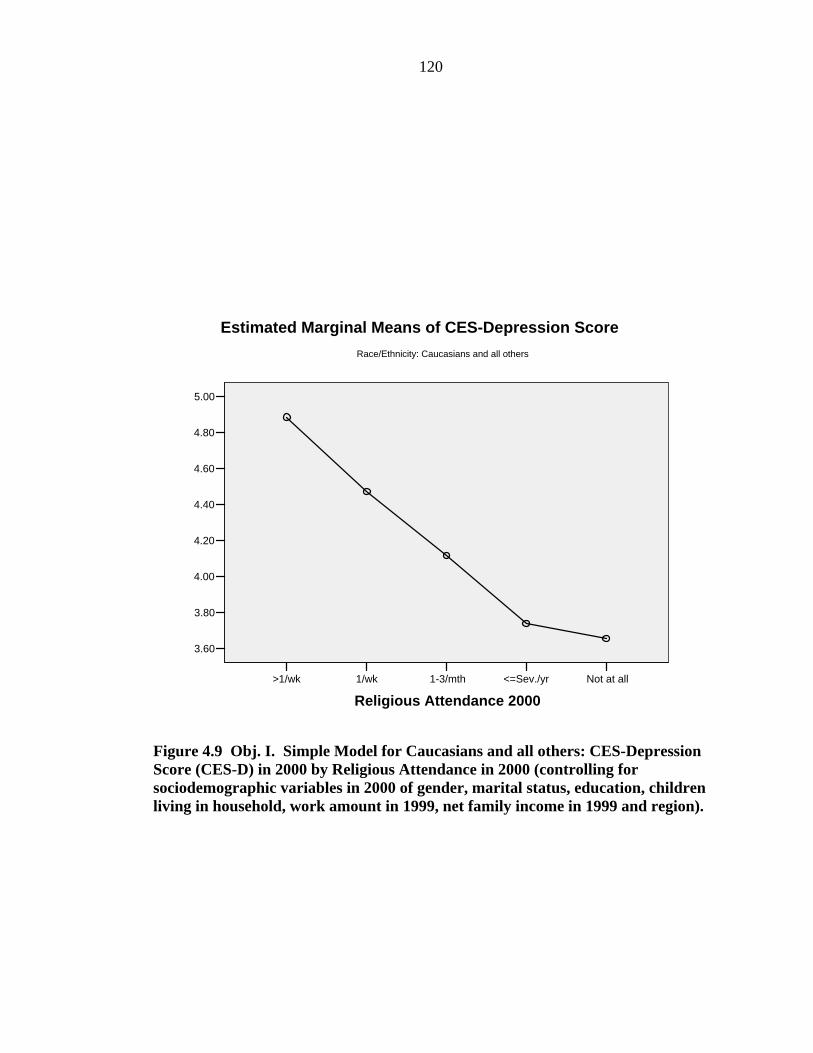
120
Figure 4.9 Obj. I. Simple Model for Caucasians and all others: CES-Depression Score (CES-D) in 2000 by Religious Attendance in 2000 (controlling for sociodemographic variables in 2000 of gender, marital status, education, children living in household, work amount in 1999, net family income in 1999 and region).
Not at all <=Sev./yr1-3/mth1/wk>1/wk Religious Attendance 2000
5.00
4.80
4.60
4.40
4.20
4.00
3.80
3.60
Race/Ethnicity: Caucasians and all others
Estimated Marginal Means of CES-Depression Score

121
Discussion Section Objective I
Objective I Summary of Findings:
Objective I.1 Religious Attendance and Physical Health Results Summary
With respect to Objective I, investigating the cross-sectional analysis of religious
attendance on physical health, mental health, and depression for the year 2000, the
following overall trends were found. For the Physical Health Composite Score (PCS),
frequency of religious attendance was found to have a curvilinear association with
physical health, in a simple model with the presence of sociodemographic control
variables in 2000 (including gender, race/ethnicity, marital status, education, number
of children living in the household, work amount in 1999, net family income in 1999,
region and residence; refer to Table 4.10). The lowest physical health scores occurred
at the two extremes of attendance, more than once per week and no attendance at all
(refer to Table 4.10 and Figure 4.1).
The full model of three two-way interactions of low work amount (part-time or less) in
the past calendar year 1999, low education in the year 2000 (less than high school),
and lowest 25 percent net family income level in the past calendar year (less than
$20,600), with religious attendance in the year 2000 reveals a curvilinear trend as
well, particularly with lowest mean physical health scores at the level of no attendance
(refer to Table A.2, Table A.2, Figure A.4, Figure A.5, and Figure A.6). In addition to
the interacting variables, the model was run in the presence of sociodemographic
control variables in 2000 including gender, race/ethnicity, marital status, and number
of children living in the household. Aside from the interactions of attendance with
work amount, education, and income, there were no significant simple main effects

122
except for number of children living in the household, which had a positive
association with physical health.
Objective I.2 Religious Attendance and Mental Health Results Summary
For the Mental Health Composite Score (MCS), frequency of religious attendance was
not significant for the simple model, in the presence of the sociodemographic control
variables previously mentioned. In the presence of interactions with race/ethnicity and
education, however, attendance was significantly associated with mental health (refer
to Table A.3). For race/ethnicity, African Americans had better mental health with
increasing frequency of attendance, whereas Caucasians and others showed the
opposite trend (refer to Figure A.7). For those with some high school or
college/graduate school education, mental health scores did not vary across attendance
levels. Respondents with less than a high school education, however, showed
differences in mental health scores with varying frequency of attendance. Those with
less than a high school education reported much lower mental health scores when
attending once per week compared with those with more education, while showing
higher mental health scores at attendance of more than once per week and one to three
times per month than those with higher education (refer to Figure A.8). The model
was run in the presence of sociodemographic controls for gender, race, marital status,
and number of children living in the household. None of these controls was significant
except for females and those with low income, which had a negative association with
mental health (refer to Table A.3).
Objective I.3 Religious Attendance and Depression Results Summary
For CES-Depression Score (CES-D), frequency of religious attendance was not
significant for the simple model, in the presence of controls. In the presence of
interactions with race/ethnicity and marital status, however, attendance was

123
significantly associated with mean depression scores (refer to Table A.4). For African
Americans, more frequent attendance was associated with lower depression scores
(being less depressed) than for Caucasians and others, which showed an opposite
trend, similar to the model with MCS (described above). For marital status, widowed
or separated respondents who attended more than once per week had much lower
scores for depression than those who did not attend, compared with the never married
group. However, the married group had higher mean scores for depression at
frequency of attendance more than once per week compared with married who never
attended (refer to Figure A.12). The model was run in the presence of
sociodemographic controls for gender, race, marital status, and number of children
living in the household. None of these controls was significant except for females, low
work, and low income; each of these variables had a negative association with
depression (refer to Table A.4).
In summary, the results indicate the following:
There was a curvilinear trend in physical health scores with increasing attendance,
controlling for the sociodemographic variables of gender, race, marital status,
education level, number of children living in the household, work amount, and
income. The highest physical health scores occurred at moderate attendance (ANOVA
F=21.8, p=0.00; refer to Table 4.10 and Figure 4.1).
For those with low socio-economic status, low education, low work amount, or low
income, some attendance was related to better physical health scores compared with
not attending at all (ANOVA F=10.9 , p=0.00; refer to Table A.1, Figure A.4, Figure
A.5 and Figure A.6).

124
African Americans who attended more frequently had better mental health or lower
depression scores, controlling for the sociodemographic variables of gender, race,
marital status, education level, number of children living in the household, work
amount, and income. In contrast, Caucasians and others who attended more frequently
had poorer mental health scores and higher depression scores.
For those with some high school or college/graduate school education, mental health
scores did not vary across attendance levels. However, respondents with less than a
high school education who attended had much better mental health scores than those
of low education who did not attend at all. The cell count for those with low education
was low, ranging from 8 to 15, so the results may not be reliable.
Objective 1.4 Religious Attendance and Mental Health and Depression Comparing
African Americans and Caucasians and All Others Results Summary
In an attempt to better understand the interactions of race/ethnicity with religious
attendance, separate regression models were run for each separate race/ethnicity for
the models with the dependent health outcomes of mental health and depression.
Similar to the overall models with the significant interaction of race/ethnicity and
religious attendance, the separate regression models by race/ethnicity showed that
African Americans who attended more frequently also reported to have better mental
health and to be less depressed compared to African Americans who did not attend.
The opposite trend occurred for Caucasians and all others. Caucasians and all others
who attended more frequently reported to have poorer mental health and to be more
depressed than Caucasians and all others who did not attend (refer to Table 4.12).
Prior research has found that African Americans derive additional non-religious
resources and support from religious participation, such as social, material, and civic
benefits (Franzini 2005). Further research to investigate the differences in mental

125
health and depression outcomes needs to be conducted to help elucidate the
differences among African Americans and Caucasians and others.
Study Strengths
National longitudinal data sets which include adequate variables on both religiousness,
and physical health, mental health, and depression are not common; most national
datasets are cross-sectional. Despite the limitations in using this secondary data set of
the NLSY79, this study is one of the few that the author is aware of that investigates
the association of religious attendance and physical health, mental health, and
depression cross-sectionally (refer to Chapter 4) and over time (refer to Chapter 5), as
well as testing the mediating theoretical pathways of behavior/lifestyle (refer to
Chapter 6) by utilizing a longitudinal national dataset. The findings of this research
contribute to the existing literature on the effects of religious attendance on physical
health, mental health, and depression because they help to clarify the association
between religious attendance and health for the 40-to-43-years age group. The present
study provides evidence that different groups, such as those of low socio-economic
status and African Americans, interact with religious attendance in different ways.
Religious attendance may serve different purposes among different groups.
Study Limitations
The limitations of the data used in this analysis include having a small number of
religious and physical and mental health variables available for a continuous number
of years throughout the study. The variables are available for only a few years during
the 25-year duration of the study. This makes it impossible to take full advantage of a
longitudinal cohort in examining changes in religiousness and health over time within
the sample. This issue will be examined in presenting Objective II.

126
A major limitation of this analysis is its cross-sectional nature, which does not permit
the assessment of causality. However, the study contributes to the current literature by
highlighting a series of interaction associations that have not been studied extensively.
Finally, in presenting Objective II of this dissertation, the longitudinal nature of the
data is explored to strengthen a possible causality argument.
Possible Policy Implications
The following policy implications are presented as possibilities based on the limited
results of this study. Further analysis in future studies and possible intervention studies
would need to be conducted before the suggested policies could be implemented.
The finding that some degree of religious participation is related to better physical
health may encourage more collaboration between the healthcare system and religious
organizations in seeking to improve the quality of life and physical health of
individuals.
Individuals of low socio-economic status (SES) who participate in religious services
appear to have better physical health than those of low SES who do not attend.
Likewise, African Americans who participate in religious services appear to have
better mental health and less depression than African Americans who do not attend.
This evidence may encourage physical and mental healthcare and other social service
agencies to collaborate with religious organizations to provide additional
“nonreligious” resources and services for the health, material, social and civic needs of
these two particular groups, those of low socio-economic status (SES) and African
Americans. However, further research is needed to further determine the nature of the

127
relationship and effects of religious participation on physical and mental health among
these two groups of low SES and African Americans.
Future Recommendations:
To build on the findings of this study, it will be important to study the effects of
religious attendance in different groups separately. A combination of quantitative and
qualitative research among different groups may provide insights into the nature of
interactions with SES, race/ethnicity, and marital status. It would be interesting to
examine different age groups to see whether similar effects are found, using different
cohorts of the National Longitudinal Survey, such as the children of the mothers of the
NLSY79.

128
CHAPTER 5 Objective II Results
Results Objective II
The Influence of Religious Attendance, Affiliation, and Change in Attendance in
early Adulthood on Mental Health, Depression, and Physical Health in Later
Adulthood
Overview of Chapter
This chapter presents the results of the analysis pertaining to Objective II, as explained
in Chapter 3. Objective II examines the relationship of religious attendance, affiliation,
and change in attendance in early adulthood to physical health, mental health, and
depression in mid-adulthood.
The chapter is organized as follows. First, I describe sample characteristics. Next, I
provide the results of several general linear models. The results of the association of
religious attendance with physical health are described first, followed by the outcomes
for mental health and, last, depression.
Sociodemographics of the Sample Population
The sociodemographic characteristics of the sample population in 1982, 1998, and
2000 included in the analysis are described below. The cohort of respondents included
in the analysis was limited to individuals who were between 22 and 25 years of age in
1982, likewise 40 and over in the year 2000 (ages 40-43).

129
Unweighted Descriptive Statistics of the Sociodemographics of the Sample Population
The unweighted sample data were used for the following reported descriptive
characteristics. Most respondents considered themselves healthy enough to work in
1981. When reporting on their health status during the year before the 1982 interview,
only 4.8 percent of respondents stated that their health could limit the amount or kind
of work for pay that they could do, while 95.2 percent stated that health would not
interfere with their work (refer to Table 5.1). Those who stated that their health would
affect their work reported most often attending religious services one to three times
per month (27.7%), while those with no health limitations most commonly reported
attending infrequently (32.4%).
In 1982, most respondents reported not being married (63.6%), about one-third
reported being married (30%), and only 6.3 percent were divorced, widowed, or
separated (refer to Table 5.1). By 1998 and 2000, most were married (about 60%), and
only about 20 percent were never married, while the remaining approximate 20
percent were divorced, widowed, or separated (compare Table 5.1 with Table 4.1 and
Table 5.4).
Education levels in 1982 indicate that most had some high school education or more
(95.8%), and only 4.2 percent reported less than a high school education. By 1998 and
2000 the education level of some high school or more increased by only about one
percent from 1982 (from 95.8% to about 96.8%; compare Table 5.4 and Table 5.1
with Table 4.1).
In 1982, most did not have children (biological, step or adopted children living in their
household, 70.6%), and about one-third reported either one or more children living

130
with them (refer to Table 5.1). By 1998, most reported having one or more children
(about two-thirds) living in their household, decreasing by about 2 percent by the year
2000 (from 68.2% to 66.8%; compare Table 4.1 to Table 5.4).
In 1982, most respondents reported working 20 or more hours per week in the
previous calendar year (73.7%), and less than one-third reported working less than 20
hours per week (26.3%; refer to Table 5.1). By 1998, those working 20 or more hours
per week increased by six percent (from 73.7% to 79.7%; refer to Table 5.4), and in
2000 by two percent (to 81.6%; refer to Table 4.1).
In 1982, approximately 80 percent of individuals reported a net family income for the
previous year of 1981(refer to Table 5.1). Most reported earning in the mid-50th
percentile range (40.9% earned $8,008 to $26,980). Approximately one-fifth reported
earning in the lowest 25th percentile, and one-fifth reported earning in the top 25th
percentile (approximately one-fifth did not report their income; refer to Table 5.1).
The percentage of respondents in each category of income percentiles reported for the
1997 and 1999 calendar years was similar to the percentage reported in each category
for the year 1981 (compare Table 5.1 with Table 5.1 Table 4.1). Note that, within just
a two-year period, the income ranges were actually higher in 1997 than in 1999 for the
lowest 25th, mid-50th, and top 25th percentile levels. For example, the lowest 25th
percentile income range in 1997 was $0 to $24,960, compared with $0 to $20,516 in
1999; the mid-50th percentile income range in 1997 was $25,000 to $71,100,
compared with $20,600 to $69,800 in 1999; and the top 25th percentile income range
in 1997 was $71,136 or more, compared with $70,000 or more in 1999. It is unclear
why net family incomes within the two lowest percentiles decreased from 1997 to
1999.

131
Most respondents lived in the same region of the United States from 1982 to 1998 and
2000 (refer to Table 5.1, Table 5.4, and Table 4.4). Most reported living in the South
(37.5%) in 1982. This increased by about two percentage points in 2000, while the
region with the lowest reported level in 1982, the Northeast (18.1%), decreased by
about two percentage points in 2000 (to 16.2%).
Most individuals reported living in an urban setting in 1982 (81.6%) versus a rural
setting (18.4%; refer to Table 5.1). By 1998 those living in an urban area decreased by
about 5 percent from 1982 (from 81.6% in 1982 to 70.4% in 1998), while those living
in a rural area in 1998 increased by over ten percent from 1982 (from 18.4% in 1982
to 29.6% in 1998; compare Table 5.4 to Table 5.1). In 2000, there was a slight trend
reversal from 1998, with a small increase in urban living of about 3 percent (from
70.4% in 1998 to 73.1% in 2000) and a decrease in rural living of about 5 percent
(from 29.4% in 1998 to 24.9% in 2000; compare Table 4.4 to Table 5.4).
Key Independent Variable: Religious Attendance in 1982 and 2000
In 1982, 31.7 percent of individuals reported attending religious services infrequently
(i.e., attending religious services less than or equal to several times a year or less; refer
to Table 5.1). For each of the demographic characteristics of 1982, the respondents
indicated that the level of “infrequent” attendance in 1982 was most commonly
reported, except for the following characteristics, those with less than a “about once
per week” (26.7 %) (during middle adulthood, ages 40-43; refer to Table 4.1).
Some of the regression models used in Objective II also controlled for 1998
sociodemographic characteristics, in addition to 1982 sociodemographic
characteristics. The 1998 sociodemographic characteristics were very similar to the

132
2000 characteristics listed in the previous chapter in the descriptives section for
Objective I (compare Table 4.1 and Table 5.4).
Weighted Descriptive Statistics of the 1982 Sociodemographics of the Sample
Population
The 1982 sociodemographic independent variable descriptives were weighted using
the 2000 sample weight. The year 2000 sample weight was used for the descriptive
statistics of the 1982 sociodemographic variables because the sample for the study was
selected in the year 2000 (J. Zagorsky, personal communication, Fall 2005).
The 2000 sample weight provides descriptions of the noninstitutionalized people born
between 1957 through 1960, living in the United States in 1978, from which the study
sample of those who turned aged 40 and over in 2000 is representative (CHRR 2004;
S. McClaskie, personal communication, Fall 2005). As previously described in
Chapter 4, the 2000 sample weight adjusted mainly for over-sampling of minorities,
particularly Hispanics and African Americans. It accounted for loss to follow-up after
the year 1979 in which the survey was administered. The weight also adjusted for two
groups which were over-sampled, military and economically disadvantaged
Caucasians. These groups were later dropped from the study in 1985 and 1991,
respectively. The sample weight did not account for the sample design effect of
clustering. This limitation would not affect the frequencies and percentages of the
weighted descriptive statistics but would only provide overly precise standard errors,
for example.
There were few differences, except for race/ethnicity, in comparison of the
percentages of the unweighted (refer to Table 5.1) and weighted (refer to Table 5.2
and Table 5.3) descriptive statistics of the 1982 sociodemographic variables. The

133
weighted descriptive statistics showed that there fewer minorities of Hispanics (6.7%)
and African Americans (13.8%) and more Caucasians and all others (79.5%) in the
United States (for those born between 1957 and 1960 who were noninstitutionalized
and living in the United States in 1978), which this study sample represented in 1982,
compared to the study sample unweighted descriptives. The unweighted descriptives
had much higher frequencies and percentages of minorities, Hispanics (18.6%),
African Americans (30.4%), and fewer Caucasians and all others (51.0%) because of
the oversampling of minorities. Oversampling of minorities was used to ensure the
study sample had adequate numbers of minorities for future statistics analyses. All
other percentage differences in each of the sociodemographic variables for the
weighted and unweighted descriptive statistics were within a plus or minus 5 %
difference (compare Table 5.1 to Table 5.2 and Table 5.3). The size of the United
States noninstitutionalized population for people living in the United States in 1978
born between 1957 and 1960 which this study sample is representative of for the
variable of religious attendance was 9.0 million people in 1982 (refer to Table 5.3).
The United States population which the sample size represented in 2000 was 9.3
million people for the variable of religious attendance. The difference in population
sizes for the survey years 1982 and 2000 occurred because more people happened to
answer the religious attendance question in 2000 than in 1982.
Weighted Descriptive Statistics of the Sociodemographics of the Sample Population
1998
The 1998 unweighted descriptive statistics were weighted using the year 2000 sample
weight. There were few differences in the unweighted compared to the weighted
descriptives statistics for the study year 1998 (compared Table 5.4 to Table 5.5 and
Table 5.6). All the sociodemographic independent variables were within a plus or
minus 5 percent difference. The only difference greater than 5% occurred for the

134
marital status level of married and living residence of urban or rural. Respondents in
the study who reported being married in 1998 were 58.4% (refer to Table 5.4), while
the weighted descriptive statistics showed 65.9% (refer to Table 5.5 and Table 5.6)
were married. Likewise, respondents who reported living in a rural (29.6%; refer to
Table 5.4) or urban (70.4%) residence in the study differed from the weighted
descriptive statistics by 5.6%. The weighted descriptives showed that 35.2% lived in a
rural residence and 64.8% lived in an urban residence (refer to Table 5.5 and Table
5.6). The size of the United States noninstitutionalized population of which this study
sample is representative was approximately 9.3 million people in 1998 who were
living in the United States in 1978 and born between the years 1957 to 1960 (refer to
Table 5.3).

135
Table 5.1 SocioDemographic Descriptives 1982 by Religious Attendance 1982 (Unweighted).
Religious Attendance 1982
>1/wk About 1/wk About 1-3/mth <=Sev./yr (Infrequent) Not at all Variable Row Total Independent Variables 1982
# Row % # Row % # Row % # Row % # Row % # Row %
Health Could Limit Work Limit or Kind 1981 Yes 9 9.6 14 14.9 26 27.7 23 24.5 22 23.4 94 4.8%
No 119 6.4 272 14.6 425 22.8 604 32.4 445 23.9 1865 95.2%
Gender Female 91 8.6 175 16.6 252 23.9 327 31.1 208 19.8 1053 51.8%
Male 44 4.5 121 12.3 214 21.8 318 32.4 283 28.9 980 48.2%
Race/Ethnicity Hispanic 33 8.7 66 17.4 77 20.3 121 31.9 82 21.6 379 18.6%
African American 38 6.1 88 14.2 180 29.1 174 28.2 138 22.3 618 30.4%
Caucasian and all others 64 6.2 142 13.7 209 20.2 350 33.8 271 26.2 1036 51.0%
Marital Divorced/Widowed/Separated 9 7.0 14 10.9 20 15.5 50 38.8 36 27.9 129 6.3% Married 43 7.0 103 16.9 141 23.1 194 31.8 129 21.1 610 30.0% Never married 83 6.4 179 13.8 304 23.5 401 31.0 326 25.2 1293 63.6%
Education >= High School 131 6.7 277 14.3 450 23.2 628 32.4 455 23.4 1941 95.8% <High School 4 4.7 18 21.2 16 18.8 14 16.5 33 38.8 85 4.2%
Child # >=2 Children 21 8.6 33 13.5 53 21.7 83 34.0 54 22.1 244 12.0% 1 Child 21 5.9 48 13.6 90 25.4 115 32.5 80 22.6 354 17.4% 0 Children 93 6.5 215 15.0 323 22.5 447 31.1 357 24.9 1435 70.6%Work Amt 1981
Full-Time (FT) > 20 hrs/wk 87 5.8 218 14.7 354 23.8 472 31.7 357 24.0 1488 73.7%
Part-Time (PT) 0 to 20 hrs/wk 46 8.6 76 14.3 110 20.7 168 31.6 132 24.8 532 26.3%
Income Net Family 1981 Missing 23 6.6 51 14.7 90 25.9 97 28.0 86 24.8 347 17.1%
Top 25% ($27,000- 75,001) 26 6.1 52 12.2 94 22.1 134 31.5 120 28.2 426 21.0% Mid 50% ($8,008 – 26,980) 57 6.9 123 14.8 204 24.5 243 29.2 204 24.5 831 40.9% Lowest 25% ($0-8,000) 29 6.8 70 16.3 78 18.2 171 39.9 81 18.9 429 21.1%

136
Table 5.1 (Continued).
Religious Attendance 1982
>1/wk About 1/wk About 1-3/mth <=Sev./yr (Infrequent) Not at all Variable Row Total Independent Variables 1982
# Row % # Row % # Row % # Row % # Row % # Row %
Region West 21 5.3 58 14.8 73 18.6 121 30.8 120 30.5 393 19.4%
South 68 9.0 106 14.0 219 28.9 211 27.8 154 20.3 758 37.5%
North Central 33 6.5 84 16.6 110 21.8 171 33.9 107 21.2 505 25.0%
Northeast 13 3.6 47 12.8 60 16.4 137 37.4 109 29.8 366 18.1%
Residence Rural 25 7.0 56 15.8 67 18.9 108 30.4 99 27.9 355 18.4% Urban 108 6.9 229 14.5 364 23.1 499 31.7 375 23.8 1575 81.6%
Religious Attendance Total 135 6.6 296.0 14.6 466.0 22.9 645.0 31.7 491.0 24.2 2033 100.0%

137
Table 5.2 SocioDemographic Descriptives 1982 by Religious Attendance 1982 Weighted (2000 sample weight divided by mean sample weight to obtain original sample size of approximately 2102 in order to directly compare frequency and percentage of each variable with the unweighted descriptive statistics).a, b
Religious Attendance 1982
>1/wk About 1/wk About 1-3/mth <=Sev./yr (Infrequent) Not at all Variable Row Total Independent Variables 1982
# Row % # Row % # Row % # Row % # Row % # Row %
Health Could Limit Work Limit or Kind 1981 Yes 11 12.1 16 16.8 21 22.5 23 25.3 22 23.3 93 4.7
No 114 6.1 254 13.4 393 20.8 639 33.9 486 25.8 1886 95.3
Gender Female 80 8.1 160 16.1 222 22.4 315 31.8 214 21.6 991 48.6
Male 49 4.7 119 11.4 203 19.4 361 34.4 315 30.1 1047 51.4
Race/Ethnicity Hispanic 12 8.7 23 16.7 24 18.0 45 32.9 32 23.7 136 6.7
African American 17 6.1 39 13.9 78 27.8 81 28.9 66 23.3 281 13.8
Caucasian and all others 100 6.2 217 13.4 323 19.9 550 33.9 431 26.6 1620 79.5
Marital Divorced/Widowed/Separated 7 6.2 13 11.3 16 14.0 43 37.7 35 30.9 114 5.6 Married 41 6.2 106 16.2 144 21.9 207 31.6 158 24.1 656 32.2 Never married 81 6.4 160 12.6 265 20.9 426 33.6 335 26.5 1267 62.2
Education >= High School 127 6.4 269 13.6 418 21.2 669 33.9 489 24.8 1972 97.1 <High School 3 4.5 9 14.6 7 11.7 5 7.7 36 61.5 58 2.9
Child # >=2 Children 15 7.8 31 15.7 40 20.4 65 32.9 46 23.3 196 9.6 1 Child 20 6.3 44 13.8 74 23.2 95 29.8 86 27.0 318 15.6 0 Children 94 6.2 204 13.4 312 20.5 517 33.9 397 26.1 1524 74.8
Work Amt 1981 Full-Time (FT) > 20 hrs/wk 79 5.1 215 13.9 342 22.0 511 33.0 404 26.0 1552 76.7
Part-Time (PT) 0 to 20 hrs/wk 46 9.8 62 13.1 81 17.3 158 33.6 124 26.3 471 23.3

138
Table 5.2 (Continued).
Religious Attendance 1982
>1/wk About 1/wk About 1-3/mth <=Sev./yr (Infrequent) Not at all Variable Row Total Independent Variables 1982
# Row % # Row % # Row % # Row % # Row % # Row %
Income Net Family 1981 Missing 17 5.5 46 14.6 72 23.1 89 28.4 89 28.9 314 15.4
Top 25% ($27,000- 75,001) 25 6.7 44 11.8 71 19.1 122 32.9 109 29.4 370 18.2 Mid 50% ($8,008 – 26,980) 54 6.5 113 13.4 193 22.9 258 30.7 223 26.5 841 41.3 Lowest 25% ($0-8,000) 33 6.4 76 14.9 89 17.4 207 40.3 108 21.0 513 25.2 West 18 5.2 39 11.0 56 16.0 112 31.8 126 35.9 352 17.3
South 64 9.4 92 13.5 178 26.2 189 27.8 156 23.0 677 33.4
North Central 38 6.3 99 16.3 129 21.3 210 34.5 132 21.6 608 30.0
Northeast 9 2.3 48 12.3 59 15.1 161 41.1 115 29.2 392 19.3
Rural 26 6.2 65 15.7 70 17.1 131 31.9 119 29.0 410 21.0 Urban 103 6.7 206 13.3 333 21.6 510 33.0 393 25.4 1545 79.0
Religious Attendance Total 129 6.3 279 13.7 425 20.9 676 33.2 529 25.9 2038 100.0a The 2000 weight adjusts for loss to follow-up after the year 1979 in which the survey was administered through the year 2000. The sample 2000 weight adjusts for over-sampling of minorities, particularly Hispanics and African Americans. The weight also adjusts for two groups that were over-sampled and later dropped from the study. In 1985 an over-sample of approximately 1000 military personnel were dropped while 200 remained in the sample. In 1991 the over-sample of economically disadvantaged Caucasians was dropped from the study. The above descriptive statistics describe those individuals who were aged 40 and over in the year 2000, from a sample designed to be representative of noninstitutionalized people born between 1957 through 1964, living in the United States in 1978 (S. McClaskie, personal communication, Fall 2005). b The year 2000 sample weight is used for the descriptive statistics of the 1982 sociodemographic variables because the sample for the study is selected in the year 2000 (J. Zagorsky, personal communication, Fall 2005).

139
Table 5.3 SocioDemographic Descriptives 1982 by Religious Attendance 1982 Weighted (2000 sample weight used to obtain descriptive statistics of the noninstitutionalized U.S. population living in the U.S. in 1978 who were born between 1957 and 1964 and turned 40 and over in the year 2000).a, b
Religious Attendance 1982
>1/wk About 1/wk About 1-3/mth <=Sev./yr (Infrequent) Not at all Variable Row Total Independent Variables 1982
# Row % # Row % # Row % # Row % # Row % # Row %
Health Could Limit Work Limit or Kind 1981 Yes
49930 12.1 69059 16.8 92618 22.5 104073 25.3 95764 23.3 411444 4.7
No 506338 6.1 1125076 13.4 1742520 20.8 2834952 33.9 2156624 25.8 8365510 95.3
Gender Female 355809 8.1 707723 16.1 983992 22.4 1399125 31.8 947812 21.6 4394462 48.6
Male 218279 4.7 528089 11.4 902630 19.4 1600086 34.4 1397528 30.1 4646611 51.4
Race/Ethnicity Hispanic 52643 8.7 101125 16.7 108480 18.0 198644 32.9 143371 23.7 604263 6.7
African American 75652 6.1 173291 13.9 346725 27.8 360938 28.9 291304 23.3 1247910 13.8
Caucasian and all others 445793 6.2 961396 13.4 1431416 19.9 2439629 33.9 1910665 26.6 7188899 79.5
Marital Divorced/Widowed/Separated 31362 6.2 57112 11.3 70734 14.0 191053 37.7 156387 30.9 506647 5.6 Married 181232 6.2 470340 16.2 637621 21.9 920397 31.6 701154 24.1 2910745 32.2 Never married 361494 6.4 708360 12.6 1177237 20.9 1887762 33.6 1487799 26.5 5622652 62.2
Education >= High School 562362 6.4 1191850 13.6 1856385 21.2 2967812 33.9 2168627 24.8 8747037 97.1 <High School 11725 4.5 37828 14.6 30236 11.7 19976 7.7 159593 61.5 259358 2.9
Child # >=2 Children 67656 7.8 136903 15.7 177679 20.4 286621 32.9 202731 23.3 871590 9.6 1 Child 88095 6.3 195057 13.8 326370 23.2 419664 29.8 380327 27.0 1409513 15.6
0 Children 418337 6.2 903852 13.4 1382572 20.5 2292927 33.9 1762282 26.1 6759970 74.8Work Amt 1981
Full-Time (FT) > 20 hrs/wk 352210 5.1 955111 13.9 1517383 22.0 2269127 33.0 1791719 26.0 6885550 76.7
Part-Time (PT) 0 to 20 hrs/wk 204066 9.8 274018 13.1 360761 17.3 700641 33.6 548095 26.3 2087582 23.3

140
Table 5.3 (Continued).
Religious Attendance 1982
>1/wk About 1/wk About 1-3/mth <=Sev./yr (Infrequent) Not at all Variable Row Total Independent Variables 1982
# Row % # Row % # Row % # Row % # Row % # Row %
Income Net Family 1981 Missing 77079 5.5 203367 14.6 320849 23.1 395143 28.4 395231 28.4 1391669 15.4
Top 25% ($27,000- 75,001) 110686 6.7 194634 11.8 314247 19.1 540230 32.9 482976 29.4 1642774 18.2 Mid 50% ($8,008 – 26,980) 241411 6.5 499871 13.4 855586 22.9 1146245 30.7 989351 26.5 3732464 41.3 Lowest 25% ($0-8,000) 144911 6.4 337940 14.9 395940 17.4 917593 40.3 477782 21.0 2274166 25.2Region West 81965 5.2 172408 11.0 250583 16.0 495919 31.8 560752 35.9 1561626 17.3
South 282797 9.4 406565 13.5 788595 26.2 836826 27.8 690409 23.0 3005192 33.4
North Central 169240 6.3 441225 16.3 574045 21.3 930786 34.5 583857 21.6 2699152 30.0
Northeast 40086 2.3 214442 12.3 262938 15.1 715415 41.1 508342 29.2 1741223 19.3
Residence Rural 113199 6.2 286224 15.7 310954 17.1 580193 31.9 527398 29.0 1817967 21.0 Urban 456015 6.7 913077 13.3 1476978 21.6 2262860 33.0 1743626 25.4 6852556 79.0
Religious Attendance Total 574088 6.3 1235812 13.7 1886621 20.9 2999211 33.2 2345340 25.9 9041073 100.0a The 2000 weight adjusts for loss to follow-up after the year 1979 in which the survey was administered through the year 2000. The sample 2000 weight adjusts for over-sampling of minorities, particularly Hispanics and African Americans. The weight also adjusts for two groups that were over-sampled and later dropped from the study. In 1985 an over-sample of approximately 1000 military personnel were dropped while 200 remained in the sample. In 1991 the over-sample of economically disadvantaged Caucasians was dropped from the study. The above descriptive statistics describe those individuals who were aged 40 and over in the year 2000, from a sample designed to be representative of noninstitutionalized people born between 1957 through 1964, living in the United States in 1978 (S. McClaskie, personal communication, Fall 2005). b The year 2000 sample weight is used for the descriptive statistics of the 1982 sociodemographic variables because the sample for the study is selected in the year 2000 (J. Zagorsky, personal communication, Fall 2005).

141
Table 5.4 Descriptives of 1998 Sociodemographics (Unweighted).
Table Total Independent Sociodemographic Variables 1998
# Row %
Marital Status Widowed/Separated /Divorce 416 21.2%
Married 1145 58.4% Never married 398 20.3% Education >=High School 1897 96.8%
- < High School 62 3.2%
Children living in household
>=2 children 988 50.4%
1 child 349 17.8% 0 children 622 31.8% Work Amt. 1997 Full-time
(>20 hrs/wk) 1549 79.7%
Part-time (0-20 hrs/wk) 394 20.3%
Net Family Income 1997 Missing 519 24.7% Top 25%
(>=$71,136 398 18.9%
Mid-50% ($25,000 to $71,100) 795 37.8%
Lowest 25% (<=$24,960) 390 18.6%
Region West 380 19.9% South 746 39.1% North Central 469 24.6% Northeast 314 16.4% Residence Rural 568 29.6% Urban 1354 70.4% Study Sample Total 2102 100.0%
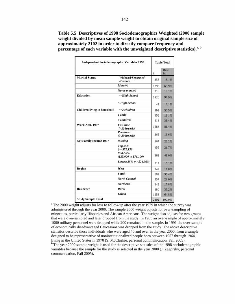
142
Table 5.5 Descriptives of 1998 Sociodemographics Weighted (2000 sample weight divided by mean sample weight to obtain original sample size of approximately 2102 in order to directly compare frequency and percentage of each variable with the unweighted descriptive statistics).a, b
Table Total Independent Sociodemographic Variables 1998
# Row %
Marital Status Widowed/Separated /Divorce 355 18.1%
Married 1295 65.9% Never married 316 16.1% Education >=High School 1926 97.9%
- < High School 41 2.1%
Children living in household >=2 children 992 50.5% 1 child 356 18.1% 0 children 618 31.4% Work Amt. 1997 Full-time
(>20 hrs/wk) 1588 81.4%
Part-time (0-20 hrs/wk) 362 18.6%
Net Family Income 1997 Missing 467 22.2% Top 25%
(>=$71,136 456 21.7%
Mid-50% ($25,000 to $71,100) 862 41.0%
Lowest 25% (<=$24,960) 317 15.1%
Region West 342 17.8% South 682 35.4% North Central 557 29.0% Northeast 343 17.8% Residence Rural 680 35.2% Urban 1253 64.8% Study Sample Total 2102 100.0%
a The 2000 weight adjusts for loss to follow-up after the year 1979 in which the survey was administered through the year 2000. The sample 2000 weight adjusts for over-sampling of minorities, particularly Hispanics and African Americans. The weight also adjusts for two groups that were over-sampled and later dropped from the study. In 1985 an over-sample of approximately 1000 military personnel were dropped while 200 remained in the sample. In 1991 the over-sample of economically disadvantaged Caucasians was dropped from the study. The above descriptive statistics describe those individuals who were aged 40 and over in the year 2000, from a sample designed to be representative of noninstitutionalized people born between 1957 through 1964, living in the United States in 1978 (S. McClaskie, personal communication, Fall 2005). b The year 2000 sample weight is used for the descriptive statistics of the 1998 sociodemographic variables because the sample for the study is selected in the year 2000 (J. Zagorsky, personal communication, Fall 2005).

143
Table 5.6 Descriptives of 1998 Sociodemographics Weighted (2000 sample weight used to obtain descriptive statistics of the noninstitutionalized U.S. population living in the U.S. in 1978 who were born between 1957 and 1964 and turned 40 and over in the year 2000).a, b
Table Total Independent Sociodemographic Variables 1998
# Row %
Marital Status Widowed/Separated /Divorce 1575902 18.1%
Married 5745051 65.9% Never married 1402719 16.1% Education >=High School 8543597 97.9%
- < High School 180075 2.1%
Children living in household >=2 children 4401216 50.5% 1 child 1580602 18.1% 0 children 2741855 31.4% Work Amt. 1997 Full-time
(>20 hrs/wk) 7045035 81.4%
Part-time (0-20 hrs/wk) 1607783 18.6%
Net Family Income 1997 Missing 2072594 22.2% Top 25%
(>=$71,136 2022731 21.7%
Mid-50% ($25,000 to $71,100) 3824995 41.0%
Lowest 25% (<=$24,960) 1405078 15.1%
Region West 1517603 17.8% South 3023914 35.4% North Central 2471912 29.0% Northeast 1522840 17.8% Residence Rural 3018050 35.2% Urban 5558459 64.8% US population of which Study Sample is Representative 9311040 100.0%
a The 2000 weight adjusts for loss to follow-up after the year 1979 in which the survey was administered through the year 2000. The sample 2000 weight adjusts for over-sampling of minorities, particularly Hispanics and African Americans. The weight also adjusts for two groups that were over-sampled and later dropped from the study. In 1985 an over-sample of approximately 1000 military personnel were dropped while 200 remained in the sample. In 1991 the over-sample of economically disadvantaged Caucasians was dropped from the study. The above descriptive statistics describe those individuals who were aged 40 and over in the year 2000, from a sample designed to be representative of noninstitutionalized people born between 1957 through 1964, living in the United States in 1978 (S. McClaskie, personal communication, Fall 2005). b The year 2000 sample weight is used for the descriptive statistics of the 1998 sociodemographic variables because the sample for the study is selected in the year 2000 (J. Zagorsky, personal communication, Fall 2005).

144
Other Control Variables included in the analysis
Religious Affiliation 1982 compared with 2000
Religious affiliation between 1982 and 2000 remained fairly constant, with a slight
decrease of 1 to 4 percentage points in each denomination (compare Table 5.7 with
Table 4.4). More than half were Protestant in both 1982 and 2000 (53.1% and 54.4%
respectively), about one third were Catholic (32% in 1982 and 28.1% in 2000), and
about one tenth reported no affiliation (10.9% in 1982 and 10.4% in 2000). The only
increase among affiliations occurred within the overall category of “Other” (from
1.8% in 1982 to 7.4% in 2000 (compare Table 5.7 with Table 4.4).
The highest attendance rate reported in 1982 across most religious affiliations was
infrequent attendance (refer to Table 5.7). Exceptions were found in the Protestant
denomination of Baptist, with most common attendance at about once to three times
per month (30.8%); affiliation reported as “Other,” with most common attendance of
more than once per week (25.8%); and no affiliation, with most common attendance in
1982 of not at all (68.3%).
By 2000, the attendance rate increased to about once per week for most affiliations
(except for Baptist and Episcopalian/Presbyterian (grouped together), who attended
most frequently, about one to three times per month in 2000).
The other exception in attendance among affiliations in 1982 was that among those
who reported no religious affiliation, most commonly reported attending religious
services not at all (68.3%). This is in contrast to the 2000 reported attendance levels
among those with no religious affiliation. Those who reported no affiliation in the
calendar year 2000, curiously reported attending most often (70.5%) among the

145
possible attendance levels. This provides evidence of possible misclassification bias
for the attendance level “not at all” for those with no religious affiliation.
For the entire sample of the NSLY79, approximately 96 percent of all respondents
were raised in some religion, while 89 percent had a religious affiliation in 1979 and
1982. Religious service attendance appeared to have increased with the aging of the
cohort. For example, the frequency of religious attendance for the category of more
than once a week more than doubled for the cohort, from 9.4 percent in 1979 to 20.1
percent in 2000 (CHRR, 2004). A similar trend was found among the sub-cohort of
the 2000 health module; attendance at more than once per week increased over
threefold from 6.6 percent in 1982 to 20.7 percent in 2000 (compare Table 5.7 with
Table 4.4). The most frequent attendance level also increased, from infrequent in 1982
(31.7%) to about once per week in 2000 (26.7%).
Weighted Descriptive Statistics for Religious Affiliation 1982
The 1982 unweighted descriptive statistics of religious affiliation were weighted using
the year 2000 sample weight. There were few differences in the unweighted compared
to the weighted descriptives statistics for the various religious affiliations, within a
plus or minus 5 percent difference (compare Table 5.7 to Table 5.8 and Table 5.9).
The only difference greater than 5 % occurred for the religious affiliation of Baptists.
Respondents in the study who reported being affiliated as a Baptist in 1982 were
51.9% (refer to Table 5.7), while the weighted descriptive statistics show 11.1% fewer
were actually Baptists, 40.8% (refer to Table 5.8 and Table 5.9).

146
Table 5.7 Religious Affiliation by Religious Attendance in 1982 (Unweighted).
Religious Attendance 1982
Religious Affiliation 1982 >1/wk About 1/wk
About 1-3/mth
<= Several times/yr
(Infrequent) Not at all
Variable Row Total
# Row
% # Row
% # Row
% # Row % # Row
% # Row % Religious Affiliation Protestant Total 105 9.5% 157 14.2% 310 28.0% 337 30.4% 198 17.9% 1107 54.4%
Baptist 45 7.8% 80 13.9% 177 30.8% 165 28.7% 107 18.6% 574 51.9% Methodist 3 2.3% 16 12.4% 40 31.0% 44 34.1% 26 20.2% 129 11.7% Lutheran 3 3.1% 8 8.2% 31 32.0% 38 39.2% 17 17.5% 97 8.8% Presbyterian 0 0.0% 2 4.4% 15 33.3% 16 35.6% 12 26.7% 45 4.1% Episcopalian 1 4.0% 2 8.0% 3 12.0% 14 56.0% 5 20.0% 25 2.3% Other 48 25.8% 42 22.6% 36 19.4% 38 20.4% 22 11.8% 186 16.8% No Denomination 5 9.8% 7 13.7% 8 15.7% 22 43.1% 9 17.6% 51 4.6%
Religious Affiliation Other than Protestant Roman Catholic
18 2.8% 132 20.2% 138 21.1% 233 35.7% 132 20.2% 653 32.1%
Jewish 1 5.6% 2 11.1% 1 5.6% 11 61.1% 3 16.7% 18 0.9% Other 9 25.0% 4 11.1% 2 5.6% 13 36.1% 8 22.2% 36 1.8% None 2 0.9% 1 0.5% 15 6.9% 51 23.4% 149 68.3% 218 10.7%
Religious Attendance Total 135 6.6% 296 14.6% 466 22.9% 645 31.7% 491 24.2% 2033 100.0%
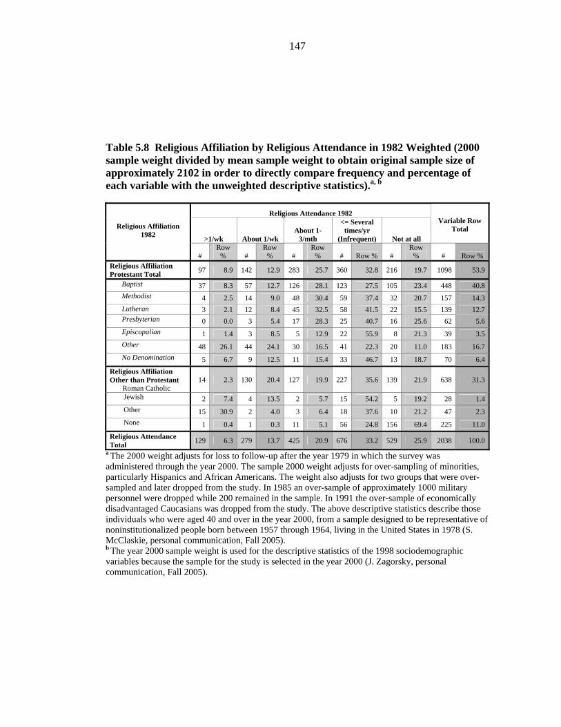
147
Table 5.8 Religious Affiliation by Religious Attendance in 1982 Weighted (2000 sample weight divided by mean sample weight to obtain original sample size of approximately 2102 in order to directly compare frequency and percentage of each variable with the unweighted descriptive statistics).a, b
Religious Attendance 1982
Religious Affiliation 1982 >1/wk About 1/wk
About 1-3/mth
<= Several times/yr
(Infrequent) Not at all
Variable Row Total
# Row
% # Row
% # Row
% # Row % # Row
% # Row % Religious Affiliation Protestant Total 97 8.9 142 12.9 283 25.7 360 32.8 216 19.7 1098 53.9
Baptist 37 8.3 57 12.7 126 28.1 123 27.5 105 23.4 448 40.8 Methodist 4 2.5 14 9.0 48 30.4 59 37.4 32 20.7 157 14.3 Lutheran 3 2.1 12 8.4 45 32.5 58 41.5 22 15.5 139 12.7 Presbyterian 0 0.0 3 5.4 17 28.3 25 40.7 16 25.6 62 5.6 Episcopalian 1 1.4 3 8.5 5 12.9 22 55.9 8 21.3 39 3.5 Other 48 26.1 44 24.1 30 16.5 41 22.3 20 11.0 183 16.7 No Denomination 5 6.7 9 12.5 11 15.4 33 46.7 13 18.7 70 6.4Religious Affiliation Other than Protestant Roman Catholic
14 2.3 130 20.4 127 19.9 227 35.6 139 21.9 638 31.3
Jewish 2 7.4 4 13.5 2 5.7 15 54.2 5 19.2 28 1.4 Other 15 30.9 2 4.0 3 6.4 18 37.6 10 21.2 47 2.3 None 1 0.4 1 0.3 11 5.1 56 24.8 156 69.4 225 11.0Religious Attendance Total 129 6.3 279 13.7 425 20.9 676 33.2 529 25.9 2038 100.0
a The 2000 weight adjusts for loss to follow-up after the year 1979 in which the survey was administered through the year 2000. The sample 2000 weight adjusts for over-sampling of minorities, particularly Hispanics and African Americans. The weight also adjusts for two groups that were over-sampled and later dropped from the study. In 1985 an over-sample of approximately 1000 military personnel were dropped while 200 remained in the sample. In 1991 the over-sample of economically disadvantaged Caucasians was dropped from the study. The above descriptive statistics describe those individuals who were aged 40 and over in the year 2000, from a sample designed to be representative of noninstitutionalized people born between 1957 through 1964, living in the United States in 1978 (S. McClaskie, personal communication, Fall 2005). b The year 2000 sample weight is used for the descriptive statistics of the 1998 sociodemographic variables because the sample for the study is selected in the year 2000 (J. Zagorsky, personal communication, Fall 2005).

148
Table 5.9 Religious Affiliation by Religious Attendance in 1982 Weighted (2000 sample weight used to obtain descriptive statistics of the noninstitutionalized U.S. population living in the U.S. in 1978 who were born between 1957 and 1964 and turned 40 and over in the year 2000).a, b
Religious Attendance 1982 Religious Affiliation
1982 >1/wk About 1/wk About 1-3/mth <= Several times/yr
(Infrequent) Not at all Variable Row Total
# Row
% # Row
% # Row
% # Row
% # Row
% # Row % Religious Affiliation Protestant Total 431670 8.9 630340 12.9 1253669 25.7 1598327 32.8 959068 19.7 4873072 53.9
Baptist 165670 8.3 251623 12.7 559133 28.1 546833 27.5 464926 23.4 1988186 40.8 Methodist 17753 2.5 62586 9.0 211806 30.4 260941 37.4 143991 20.7 697077 14.3 Lutheran 13156 2.1 51890 8.4 200714 32.5 256803 41.5 95937 15.5 618501 12.7 Presbyterian 0 0.0 14676 5.4 77581 28.3 111338 40.7 70106 25.6 273701 5.6 Episcopalian 2344 1.4 14482 8.5 22041 12.9 95671 55.9 36485 21.3 171022 3.5 Other 212022 26.1 196085 24.1 134546 16.5 181508 22.3 89286 11.0 813447 16.7 No Denomination 20724 6.7 38997 12.5 47847 15.4 145233 46.7 58337 18.7 311138 6.4

149
Table 5.9 (Continued).
Religious Attendance 1982 Religious Affiliation
1982 >1/wk About 1/wk About 1-3/mth <= Several times/yr
(Infrequent) Not at all Variable Row Total
# Row
% # Row
% # Row
% # Row
% # Row
% # Row % Religious Affiliation Other than Protestant Roman Catholic
64120 2.3 576821 20.4 561803 19.9 1007355 35.6 618809 21.9 2828908 31.3
Jewish 9182 7.4 16821 13.5 7134 5.7 67610 54.2 23922 19.2 124669 1.4 Other 65001 30.9 8454 4.0 13465 6.4 79057 37.6 44541 21.2 210518 2.3 None 4115 .4 3376 .3 50551 5.1 246862 24.8 691352 69.4 996257 11.0
U.S. Population of which Study Sample is Representative for Religious Attendance
574088 6.3 1235812 13.7 1886621 20.9 2999211 33.2 2345340 25.9 9041073 100.0
a The 2000 weight adjusts for loss to follow-up after the year 1979 in which the survey was administered through the year 2000. The sample 2000 weight adjusts for over-sampling of minorities, particularly Hispanics and African Americans. The weight also adjusts for two groups that were over-sampled and later dropped from the study. In 1985 an over-sample of approximately 1000 military personnel were dropped while 200 remained in the sample. In 1991 the over-sample of economically disadvantaged Caucasians was dropped from the study. The above descriptive statistics describe those individuals who were aged 40 and over in the year 2000, from a sample designed to be representative of noninstitutionalized people born between 1957 through 1964, living in the United States in 1978 (S. McClaskie, personal communication, Fall 2005). b The year 2000 sample weight is used for the descriptive statistics of the 1998 sociodemographic variables because the sample for the study is selected in the year 2000 (J. Zagorsky, personal communication, Fall 2005).

150
Change in Religious Attendance 1982 to 2000
A variable was created to account for changes in religious attendance from 1982 to
2000. Seven levels were created to account for such changes between 1982 and 2000,
based on the same five attendance levels for each period. The five levels of attendance
were: (1) more than once per week, (2) about once per week, (3) about one to three
times per month, (4) less than or equal to several times per year, and (6) not at all. For
the change in attendance variable, the seven levels include: (1) high increase in
attendance, with a difference in attendance levels from 1982 to 2000 of +3 to +4; (2)
low increase in attendance, with a difference in attendance levels from 1982 to 2000 of
+1 to +2; (3) no change in high attendance from 1982 to 2000, with the attendance
level remaining at more than once per week to once per week; (4) no change in
moderate attendance from 1982 to 2000, with the attendance level remaining at one to
three times per month; (5) no change in low attendance from 1982 to 2000, with the
attendance level remaining at infrequent to not at all; (6) low decrease in attendance
from 1982 to 2000, with a difference in attendance levels from 1982 to 2000 of -1 or
-2; and last, (7) high decrease in attendance, with a difference in the attendance levels
from 1982 to 2000 of -3to -4.
Among the seven levels of this variable of change in attendance, according to a one-
way Analysis of Variance ([ANOVA]; without controlling for other factors), the level
which had the highest health score for physical and mental health and lowest
depression score was within the level of no change in moderate attendance (attending
one to three times per month), from 1982 to 2000: PCS (52.7), MCS (53.6), CES-
Depression (3.1; refer to Table 5.10). The same lowest depression score also occurred
at high decrease in attendance (refer to Table 5.10). The poorest health scores were
reported for PCS at the level of high increase in attendance from 1982 to 2000 (51.2),

151
for MCS at the level of “no change in high attendance from 1982 to 2000” (51.3), and
for CES-Depression at the level of “high increase in attendance” from 1982 to 2000,
(4.0; refer to Table 5.10, Figure 5.1, Figure 5.2, and Figure 5.3 respectively).
Correlation and Multicollinearity
Possible correlations and collinearity problems were checked for with respect to the
1982 and 1998 socio-demographic variables. Only the variables of education 1982 and
1998 and region 1982 and 1998 were found to be multicollinear. The education 1998
and region 1998 variables were excluded from the Objective II models. The religious
attendance and affiliation 1982 variables were also slightly multicollinear. Thus
attendance and affiliation were each run in separate models to observe their
relationship with the health outcome variables. Change in religious attendance from
1982 to 2000 was found to be multicollinear and correlated with both attendance and
affiliation 1982. Thus change in attendance was also run in separate models in
Objective II, in order to observe its relationship with the dependent health variables,
without the presence of attendance or affiliation.

152
Table 5.10 Descriptives and One Way ANOVA of Independent Variable Change in Religious Attendance 1982 to 2000 by Dependent Health Variables 2000 PCS, MCS and C-ESD.
Dependent Health Variable Religious Attendance Change 1982 to 2000
Statistic PCS MCS CES
D # 458 458 460 % 22.7% 22.7% 22.7
% Mean 51.2 52.0 4.0
High Increase (difference in attendance level from 1982 to 2000 is +3 or +4)
SE .4 0.4 0.2 # 686 686 690 % 34.0% 34.0% 34.1
% Mean 51.9 53.0 3.3
Low Increase (difference in attendance level from 1982 to 2000 is +1 or +2)
SE 0.3 0.3 0.2 # 57 57 57 % 2.8% 2.8% 2.8% Mean 52.3 51.3 3.9
High No Change (attendance level from 1982 to 2000 stays the same at >1/wk or 1/wk)
SE 1.1 1.5 0.8 # 148 148 148 % 7.3% 7.3% 7.3% Mean 52.7 53.6 3.1
Moderate No Change (attendance level from 1982 to 2000 stays the same at 1-3x/mth)
SE 0.6 0.6 0.3 # 125 125 125 % 6.2% 6.2% 6.2% Mean 52.3 52.5 3.5
Low No Change (attendance level from 1982 to 2000 stays at the same at infrequent or not at all)
SE 0.7 0.8 0.4 # 419 419 419 % 20.8% 20.8% 20.7
% Mean 52.4 53.0 3..3
Low Decrease (difference in attendance level from 1982 to 2000 is -1 or -2)
SE 0.4 0.4 0.2 # 124 124 125 % 6.1% 6.1% 6.2% Mean 51.6 54.0 3.1
High Decrease (difference in attendance level from 1982 to 2000 is -3 or -4)
SE 0.8 0.7 0.5 # 2017 2017 2024 % 100% 100% 100% Mean 51.9 52.8 3.5
Religious Attendance Change from 1982 to 2000 Total
SE 0.2 0.2 0.1 F Value 1.1 1.7 1.8 P-value 0.34 0.13 0.10 Between Groups df 6 6 6 Within Groups df 2010 2010 2017
Total df 2016 2016 2023

153
highdecrease inattend 82 to2000 (jumpof -3 or -4)
lowdecrease inattend 82 to2000 (jumpof -1 or -2)
no change inlow attend82 to 2000
(4,5)<=sev/yr or
notatal
no change inmoderate
attend 82 to2000 (3,4) 1-
3 x mth
no change inhigh attend82to2000
(1,2)
low increasein attend 82
to 2000 (jumpof 2 or 1)
highincrease inattend 82 to2000 (jumpof 4 or 3)
Change in Religious Attendance 1982 to 2000 categories (based on 5levels)
52.50
52.00
51.50
Mea
n of
Phy
Hlh
2000
Figure 5.1 One-Way ANOVA of Physical Health Composite Score (SF-12 PCS) in 2000 by Change in Religious Attendance 1982 to 2000 without controls.

154
highdecrease inattend 82 to2000 (jumpof -3 or -4)
lowdecrease inattend 82 to2000 (jumpof -1 or -2)
no change inlow attend82 to 2000
(4,5)<=sev/yr or
notatal
no change inmoderate
attend 82 to2000 (3,4) 1-
3 x mth
no change inhigh attend82to2000
(1,2)
low increasein attend 82
to 2000 (jumpof 2 or 1)
highincrease inattend 82 to2000 (jumpof 4 or 3)
Change in Religious Attendance 1982 to 2000 categories (based on 5levels)
54.00
53.00
52.00
51.00
Mea
n of
Men
talH
lh20
00
Figure 5.2 One-Way ANOVA, of Mental Health Composite Score (SF-12 MCS) in 2000 by Change in Religious Attendance 1982 to 2000 without controls.

155
highdecrease inattend 82 to2000 (jumpof -3 or -4)
lowdecrease inattend 82 to2000 (jumpof -1 or -2)
no change inlow attend82 to 2000
(4,5)<=sev/yr or
notatal
no change inmoderate
attend 82 to2000 (3,4) 1-
3 x mth
no change inhigh attend82to2000
(1,2)
low increasein attend 82
to 2000 (jumpof 2 or 1)
highincrease inattend 82 to2000 (jumpof 4 or 3)
Change in Religious Attendance 1982 to 2000 categories (based on 5 levels)
4.50
4.25
4.00
3.75
3.50
3.25
3.00
Mea
n of
CES
D00
Figure 5.3 One-Way ANOVA, of CES-Depression Score (CES-D) in 2000 by Change in Religious Attendance 1982 to 2000 without controls.

156
Objective II Results
The Influence of Religious Attendance, Affiliation, and Change in Attendance in
early Adulthood on Physical Health, Mental Health, and Depression in Later
Adulthood
Objective II.1. The influence of religious attendance 1982 on physical health, mental
health, and depression in 2000, controlling for 1982 sociodemographic factors.
Results for Objective II.1: The background characteristics included in this analysis are
the following socioeconomic factors (measured in 1982 ): gender, race/ethnicity,
marital status, education, number of children (living in the household with the
respondent), amount of work (hours per week) in 1981, net family income in 1981,
residence, and region, including baseline health limitations in 1981. Table 5.1 provides
a descriptive summary of the 1982 variables included in the model by 1982 religious
attendance levels. The same type of sociodemographic variables used in the model for
Objective I for the year 2000 (in the previous chapter), were used in the models for
Objective II, for the year 1982. These same type of sociodemographic variables were
retained in all subsequent models for the year 1982, even though not all the variables
were significant. Each of these variables was retained as a standard sociodemographic
variable to control for in relation to health outcomes, and for comparative purposes
pertaining to each model, in each objective.
The results of the general linear model analysis indicate that higher levels of
attendance in early adulthood are associated with better mental health and lower
depression in mid-adulthood, controlling for 1982 sociodemographic factors. Those
who attended more frequently in 1982 were less likely to report a high depression
index compared to those who reported attending not at all in 1982 (refer to Table 5.11
and Table 5.12). Gender was the only sociodemographic control variable related to

157
mental health in 2000; males reported better mental health scores compared to
females. Males were also less likely to be depressed compared to females. Other
factors associated with having higher rates of depression in 2000 were having a health
limitation (which could prevent a respondent from working for pay) in 1981, being
African American, having one or more children in 1982, and living in the South or
North Central United States in 1982 (refer to Table 5.11 and Table 5.12).
Table 5.11 Obj. II. ANOVA Simple Model of Physical Health Composite Score, (SF-12PCS), Mental Health Composite Score (SF-12 MCS), and CES-Depression Score (CES-D) in 2000 by Religious Attendance in 1982 (controlling for baseline health limitations in amount or kind of work one could do for pay in 1981 and sociodemographic variables in 1982 of gender, race/ethnicity, marital status, education, number of children living in the household, work amount in 1981, net family income in 1981 and residence and region).
Physical Health Composite Score (SF-
12 PCS) 2000
Mental Health Composite Score (SF-
12 MCS) 2000
CES-Depression Score (CES-D) 2000 Independent Variables 1982
Source df F Sig. df F Sig. df F Sig.
Corrected Model 21 4.5 .00 21 2.8 .00 21 5.9 .00
Intercept 1 4699.9 .00 1 5083.5 .00 1 162.9 .00Religious Attendance 1982 4 1.0 .39 4 2.9 .02 4 2.4 .05Health Could Limit Amt/Kind Work 1981 1 44.7 .00 1 2.1 .14 1 16.1 .00Gender 1 4.0 .05 1 22.4 .00 1 14.0 .00Race/Ethnicity 2 6.3 .00 2 .4 .66 2 6.7 .00Marital Status1982 2 .5 .63 2 .6 .55 2 .4 .70Education 1982 1 1.4 .24 1 .03 .86 1 .2 .66Child # in Household 1982 2 .7 .49 2 1.7 .18 2 7.0 .00Work Amount 1981 1 1.3 .25 1 .4 .54 1 .6 .42Net Family Income 1981 3 .4 .76 3 .9 .42 3 .8 .48Residence 1982 1 3.1 .08 1 .5 .48 1 .4 .54Region 1982 3 .7 .57 3 1.1 .34 3 2.8 .04Error 1805 1805 1811 Total 1827 1827 1833 Corrected Total 1826 1826 1832 a Adj. R Squared 0 .039 .020 0.053

158
Table 5.12 Obj. II. Parameter Estimates of Simple Model of Physical Health Composite Score, (SF-12PCS), Mental Health Composite Score (SF-12 MCS), and CES-Depression Score (CES-D) in 2000 by Religious Attendance in 1982 (controlling for baseline health limitations in amount or kind of work one could do for pay in 1981 and sociodemographic variables in 1982 of gender, race/ethnicity, marital status, education, number of children living in the household, work amount in 1981, net family income in 1981, residence and region).
Physical Health Composite Score (SF-12 PCS) 2000
Mental Health Composite Score (SF-12 MCS) 2000
CES-Depression Score (CES-D) 2000 Independent
Variables 1982 Parameter B Sig. CI 95% B Sig. CI
95% B Sig. CI 95%
Intercept 52.2 .00 49.7 54.7 54.1 .00 51.5 56.7 2.4 .00 1.11 3.72
Rel. Attend. 82 >1/wk (RA) .9 .28 -.7 2.5 2.2 .01 .4 3.9 -1.1 .01 -1.96 -.24
RA 82 1/wk 1.2 .06 .0 2.4 1.3 .04 .0 2.6 -.6 .08 -1.22 .08 RA 82 1-3x/mth .3 .55 -.8 1.5 1.7 .01 .5 2.8 -.7 .01 -1.31 -.14
RA 82<=Sev.x/yr (Infreq.)
.4 .47 -.6 1.4 1.4 .01 .3 2.5 -.5 .05 -1.06 .00
RA 82 Not at all (No) 0(a) . . . 0(a) . . . 0(a) . . .
81 Hlh Limits Amt. or Kind of Work Yes
-5.8 .00 -7.6 -4.1 -1.3 .14 -3.1 .5 1.8 .00 .94 2.73
81 Hlh Limits Amt . or Kind of Work No
0(a) . . . 0(a) . . . 0(a) . . .
Female -.8 .05 -1.6 .0 -2.0 .00 -2.9 -1.2 .8 .00 .38 1.21
Male 0(a) . . . 0(a) . . . 0(a) . . .
Hispanic -1.4 .01 -2.5 -.3 .1 .81 -1.0 1.3 .4 .22 -.22 .95 African American -1.5 .00 -2.5 -.6 -.4 .44 -1.4 .6 .9 .00 .43 1.43
Caucasian and others 0(a) . . . 0(a) . . . 0(a) . . .
Marital Status: Div./Wid./Sep. -.6 .45 -2.3 1.0 -.4 .69 -2.1 1.4 -.2 .61 -1.09 .64
Married .2 .74 -.9 1.2 -.6 .27 -1.7 .5 -.2 .43 -.77 .33
Never Married 0(a) . . . 0(a) . . . 0(a) . . . Education Level: >=High School 82
1.2 .24 -.8 3.2 .2 .86 -1.9 2.3 -.2 .66 -1.26 .80
< High School 82 0(a) . . . 0(a) . . . 0(a) . . .
>=2 Children 82 -.9 .23 -2.3 .5 -1.3 .09 -2.7 .2 1.3 .00 .59 2.06
1 Child 82 -.3 .65 -1.4 .9 .0 .98 -1.2 1.2 .8 .01 .17 1.40 No Children 82 0(a) . . . 0(a) . . . 0(a) . . .
Work Full-Time .6 .25 -.4 1.5 -.3 .54 -1.3 .7 -.2 .42 -.70 .29
Work Part-Time 0(a) . . . 0(a) . . . 0(a) . . .

159
Table 5.12 (Continued).
Physical Health Composite Score (SF-12 PCS) 2000
Mental Health Composite Score (SF-12 MCS) 2000
CES-Depression Score (CES-D) 2000 Independent
Variables 1982 Parameter B Sig. CI 95% B Sig. CI
95% B Sig. CI 95%
Income 82 Missing -.6 .33 -1.8 .6 -.9 .17 -2.2 .4 .4 .23 -.25 1.03
Income 82 Top 25% -.4 .52 -1.6 .8 -1.0 .14 -2.3 .3 .5 .15 -.17 1.11
Income 82 Mid 50% -.1 .78 -1.2 .9 -.6 .27 -1.7 .5 .3 .24 -.21 .85
Income 82 Lowest 25% 0(a) . . . 0(a) . . . 0(a) . . .
Residence 82 Urban -.9 .08 -1.9 .1 .4 .48 -.7 1.4 -.2 .54 -.69 .36
Residence 82 Rural 0(a) . . . 0(a) . . . 0(a) . . .
Region 82: West -.7 .25 -2.0 .5 -.3 .66 -1.6 1.0 .5 .13 -.15 1.17
South 82 .0 .97 -1.1 1.1 -.7 .27 -1.8 .5 .9 .00 .28 1.46 North Central 82 -.4 .53 -1.5 .8 .3 .65 -.9 1.5 .6 .07 -.04 1.17
Northeast 82 0(a) . . . 0(a) . . . 0(a) . . . a This parameter is set to zero because it is redundant.
A positive trend was observed in the association between attendance during young
adulthood to self-reported physical health in mid-adulthood, controlling for the same
1982 background factors included in the analysis of mental health and depression.
However, the difference between the different attendance levels was not significant
(refer to Table 5.11 and Table 5.12). The sociodemographic control variables in young
adulthood that were related to having poorer physical health in later adulthood
included having a health limitation in 1981; being female, African American or
Hispanic; and living in a rural residence.
In order to control for the influence of later sociodemographic variables in 1998 on
health in 2000, the following 1998 sociodemographic variables were added to the
model: marital status, number of children (living in the household with the
respondent), amount of work (hours per week) in 1997, net family income in 1997,
and residence. The 1998 variables of education and region were excluded from the

160
model, because they were found to be multicollinear with the 1982 variables of
education and region.
The results of the general linear model analysis were similar to those observed when
only 1982 controls were included in the model. Higher levels of attendance in early
adulthood were associated with better mental health and lower depression in mid-
adulthood, controlling for 1982 and 1998 sociodemographic factors (refer to ANOVA
Table B.1, Parameter Estimate Table B.2, Figure B.2, and Figure B.3). The other
factors related to better mental health in 2000 were being male and working twenty or
more hours per week in 1997. The factors related to lower levels of depression in 2000
were: not having a health limitation in 1981, being male, having no children (living
with the respondent) in 1982, living in the Northeast region of the United States in
1982, being married in 1998, working twenty or more hours in 1997, and having an
income in the range of the middle 50th to the top 25th percentile in 1997 (refer to
ANOVA Table B.1, and Parameter Estimate Table B.2).
Similar to the simple model controlling for 1982 sociodemographic variables only,
including both 1982 and 1998 control variables, a positive trend was also observed for
the association between early attendance and later physical health; however, the
association was not significant overall. Other factors that were related to better
physical health were not having a health limitation in 1981, being Caucasian, married
in 1998, and working twenty or more hours per week in 1997 (refer to ANOVA Table
B.1, Parameter Estimate Table B.2, and Figure B.1).
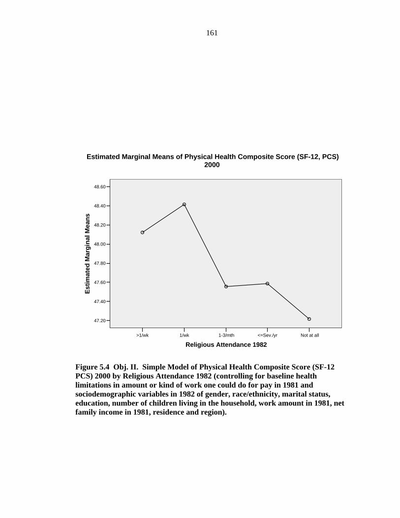
161
Not at all<=Sev./yr1-3/mth1/wk>1/wk
Religious Attendance 1982
48.60
48.40
48.20
48.00
47.80
47.60
47.40
47.20
Estim
ated
Mar
gina
l Mea
ns
Estimated Marginal Means of Physical Health Composite Score (SF-12, PCS)2000
Figure 5.4 Obj. II. Simple Model of Physical Health Composite Score (SF-12 PCS) 2000 by Religious Attendance 1982 (controlling for baseline health limitations in amount or kind of work one could do for pay in 1981 and sociodemographic variables in 1982 of gender, race/ethnicity, marital status, education, number of children living in the household, work amount in 1981, net family income in 1981, residence and region).

162
Not at all<=Sev./yr1-3/mth1/wk>1/wk
Religious Attendance 1982
53.10
52.80
52.50
52.20
51.90
51.60
51.30
51.00
50.70
Estim
ated
Mar
gina
l Mea
ns
Estimated Marginal Means of Mental Health Composite Score (SF-12, MCS)2000
Figure 5.5 Obj. II. Simple Model of Mental Health Composite Score (SF-12 MCS) 2000 by Religious Attendance 1982 (controlling for baseline health limitations in amount or kind of work one could do for pay in 1981 and sociodemographic variables in 1982 of gender, race/ethnicity, marital status, education, number of children living in the household, work amount in 1981, net family income in 1981, residence and region).

163
Not at all<=Sev./yr1-3/mth1/wk>1/wk
Religious Attendance 1982
5.20
5.00
4.80
4.60
4.40
4.20
4.00
Estim
ated
Mar
gina
l Mea
ns
Estimated Marginal Means of CES-Depression Score
Figure 5.6 Obj. II. Simple Model of CES-Depression Score (CES-Depression) 2000 by Religious Attendance 1982 (controlling for baseline health limitations in amount or kind of work one could do for pay in 1981 and sociodemographic variables in 1982 of gender, race/ethnicity, marital status, education, number of children living in the household, work amount in 1981, net family income in 1981, residence and region).

164
Results for Objective II.1
The above-mentioned regression models for the outcome variables of physical health,
mental health, and depression were run without the baseline control variable of “health
problems which could limit the amount or kind of work one could do in 1981.” The
regression models were run without this health limitations control variable because as
an independent type of health variable it may be measuring the same concept as one of
the dependent health outcome variables. In addition, because it is a very significant
independent control variable, it is important to determine whether it is driving the
significant relationship between the independent variable of religious attendance and
the dependent variables of physical health and depression (refer to Table 5.12).
The variable was created from the two survey questions “(Are you/would you be)
limited in the kind of work you (could) do on a job for pay because of your health?” as
well as the question “(Are you/would you be) limited in the amount of work you
(could) do because of your health?” with possible responses of “yes” or “no” (NLS,
2004).
This health limitation variable was significant in the simple regression models for the
dependent health variables of physical health (B= -5.8, p =0.00) and depression
(B=1.8, p=0.00), but not for mental health (B=-1.3, p = 0.14; refer to Table 5.12).
This significant variable of health limitations may subsume some of the explained
variance in physical health and depression contributed by the other independent
sociodemographic control variables. Without the presence of the health limitation
control variable, less overall variance in physical health and depression was explained
by the models, evidenced by smaller adjusted R squares, reduced by almost half for
165
the health outcome variables of physical health (reduced adjusted R2 = 0.039 to 0.021)
and depression (reduced adjusted R2 = 0.053 to 0.025; compare Table 5.11 and Table
5.13). In the presence of the independent variable of health limitations, the adjusted R
square is still low, evidence that this independent variable of health limitations is not
measuring the same concept as the dependent variable of physical health or
depression. Therefore, this provides some justification for keeping the independent
control variable of health limitations in the models.
In addition, in the absence of the health limitation control variable, some of the
remaining sociodemographic variables increased in significance, particularly for some
of the levels of religious attendance (compare Table 5.12 to Table 5.13). Religious
attendance was significant with and without the independent variable of health
limitations for the models with the dependent variables of physical health and
depression (compare Table 5.12 to Table 5.13). Therefore, this is evidence that the
variable of health limitations was not driving the significant relationship between the
independent variable of religious attendance and the dependent variables of physical
health and depression.
Other previously nonsignificant variables (in the presence of the variable of health
limitations; refer to Table 5.12) became significant in the absence of the variable of
health limitations in the models for physical health and depression. For example, for
the physical health model, in the absence of the control variable of health limitations,
the sociodemographic variable of education beyond high school, having no children
living in the household with the respondent, and working 20 or more hours per week
became significantly associated with higher (better) physical health scores (compare
Table 5.12 to Table 5.13). Also, physical health and mental health scores were higher

166
and depression scores lower across the religious attendance levels without the
presence of the health limitations control variable; compare Figure 5.4, Figure 5.5,
Figure 5.6, with Figure 5.7, Figure 5.8 and Figure 5.9).
Table 5.13 Obj. II. Parameter Estimates of Simple Model of Physical Health Composite Score, (SF-12 PCS), Mental Health Composite Score (SF-12 MCS), and CES-Depression Score (CES-D) 2000 by Religious Attendance 1982 (excluding baseline health limitations in amount or kind of work one could do for pay in 1981 and controlling for sociodemographic variables in 1982 of gender, race/ethnicity, marital status, education, number of children living in the household, work amount in 1981, net family income in 1981, residence and region).
Physical Health Composite Score (SF-12 PCS) 2000
Mental Health Composite Score (SF-12 MCS) 2000
CES-Depression Score (CES-D) 2000 Independent
Variables 1982 Parameter B Sig. CI 95% B Sig. CI
95% B Sig. CI
95%
Intercept 50.9 .00 48.4 53.4 54.0 .00 51.4 56.6 2.7 .00 1.4 4.0
Rel. Attend.1982 >1/wk (RA) .5 .57 -1.2 2.1 2.2 .01 .5 3.9 -1.1 .01 -1.9 -.2
RA 1982 1/wk 1.5 .02 .2 2.7 1.2 .08 -.1 2.5 -.5 .12 -1.2 .1
RA 1982 1-3x/mth .4 .48 -.7 1.5 1.7 .00 .6 2.9 -.8 .01 -1.4 -.2 RA1982<=Sev.x/yr (Infreq.) .6 .25 -.4 1.6 1.5 .01 .4 2.5 -.7 .02 -1.2 -.1
RA 1982 Not at all (No) 0(a) . . . 0(a) . . . 0(a) . . .
Female -.9 .02 -1.7 -.1 -2.2 .00 -3.0 -1.3 .9 .00 .5 1.3
Male 0(a) . . . 0(a) . . . 0(a) . . .
Hispanic -1.3 .02 -2.4 -.2 .0 .95 -1.1 1.2 .4 .13 -.1 1.0
African American -1.6 .00 -2.6 -.6 -.7 .19 -1.7 .3 1.0 .00 .5 1.5 Caucasian and all others 0(a) . . . 0(a) . . . 0(a) . . .
Marital Status 1982:Div/Wid/Sep -.5 .52 -2.2 1.1 -1.0 .27 -2.7 .8 -.2 .68 -1.0 .7
Married 1982 .2 .68 -.8 1.3 -.5 .37 -1.6 .6 -.3 .34 -.8 .3
Never Married 82 0(a) . . . 0(a) . . . 0(a) . . . Education Level: >=High School 1982
2.1 .04 .1 4.0 .1 .94 -1.9 2.1 -.4 .47 -1.4 .6
< High School 82 0(a) . . . 0(a) . . . 0(a) . . .
>=2 Children 82 -1.2 .09 -2.6 .2 -1.4 .06 -2.8 .1 1.4 .00 .7 2.1
1 Child 1982 -.2 .74 -1.4 1.0 .0 .99 -1.2 1.2 .8 .01 .2 1.5
No Children 82 0(a) . . . 0(a) . . . 0(a) . . . Work Full-Time 81 .8 .10 -.2 1.7 -.2 .70 -1.2 .8 -.3 .27 -.8 .2
Work Part-Time 81 0(a) . . . 0(a) . . . 0(a) . . .

167
Table 5.13 (Continued).
Physical Health Composite Score (SF-12 PCS) 2000
Mental Health Composite Score (SF-12 MCS) 2000
CES-Depression Score (CES-D) 2000 Independent
Variables 1982 Parameter B Sig. CI 95% B Sig. CI
95% B Sig. CI
95%
Income 1981 Missing -.8 .19 -2.1 .4 -.9 .17 -2.2 .4 .4 .23 -.3 1.0
Income 1981 Top 25% -.7 .28 -1.9 .6 -.9 .17 -2.2 .4 .5 .10 -.1 1.2
Income 1981 Mid 50% -.4 .50 -1.4 .7 -.7 .20 -1.8 .4 .4 .19 -.2 .9
Income 1981 Lowest 25% 0(a) . . . 0(a) . . . 0(a) . . .
Residence 1982 Urban -.9 .09 -1.9 .1 .2 .71 -.9 1.3 -.1 .61 -.7 .4
Residence 1982 Rural 0(a) . . . 0(a) . . . 0(a) . . .
Region 1982: West -.7 .25 -2.0 .5 -.1 .85 -1.5 1.2 .5 .11 -.1 1.2
South 1982 .1 .83 -1.0 1.3 -.3 .64 -1.5 .9 .7 .01 .1 1.3
North Central 82 -.4 .50 -1.6 .8 .6 .37 -.7 1.8 .5 .09 -.1 1.1
Northeast 1982 0(a) . . . 0(a) . . . 0(a) . . . Adj. R Square 0.021 0.025 0.025 Corrected Model df 20 20 20
Error df 1877 1877 1877 Total df 1898 1898 1898 F 3.1 3.4 3.4 Sig. 0.00 0.00 0.00
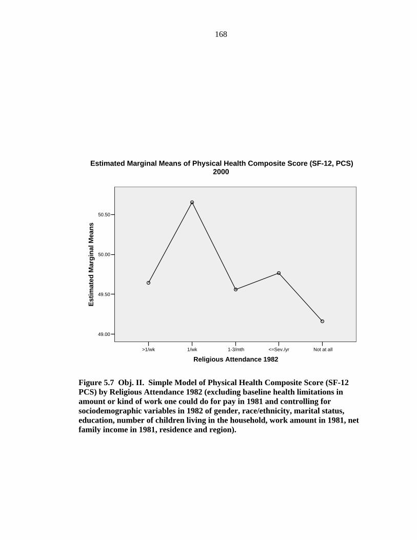
168
Not at all<=Sev./yr1-3/mth1/wk>1/wk
Religious Attendance 1982
50.50
50.00
49.50
49.00
Estim
ated
Mar
gina
l Mea
ns
Estimated Marginal Means of Physical Health Composite Score (SF-12, PCS)2000
Figure 5.7 Obj. II. Simple Model of Physical Health Composite Score (SF-12 PCS) by Religious Attendance 1982 (excluding baseline health limitations in amount or kind of work one could do for pay in 1981 and controlling for sociodemographic variables in 1982 of gender, race/ethnicity, marital status, education, number of children living in the household, work amount in 1981, net family income in 1981, residence and region).

169
Not at all<=Sev./yr1-3/mth1/wk>1/wk
Religious Attendance 1982
53.50
53.00
52.50
52.00
51.50
51.00
Estim
ated
Mar
gina
l Mea
ns
Estimated Marginal Means of Mental Health Composite Score (SF-12, MCS)2000
Figure 5.8 Obj. II. Simple Model of Mental Health Composite Score (SF-12 MCS) by Religious Attendance 1982 (excluding baseline health limitations in amount or kind of work one could do for pay in 1981 and controlling for sociodemographic variables in 1982 of gender, race/ethnicity, marital status, education, number of children living in the household, work amount in 1981, net family income in 1981, residence and region).

170
Not at all<=Sev./yr1-3/mth1/wk>1/wk
Religious Attendance 1982
4.75
4.50
4.25
4.00
3.75
3.50
Estim
ated
Mar
gina
l Mea
ns
Estimated Marginal Means of CES-Depression Score
Figure 5.9 Obj. II. Simple Model of CES-Depression Score (SF-12 CES-D) by Religious Attendance 1982 (excluding baseline health limitations in amount or kind of work one could do for pay in 1981 and controlling for sociodemographic variables in 1982 of gender, race/ethnicity, marital status, education, number of children living in the household, work amount in 1981, net family income in 1981, residence and region).

171
Objective 2.2. The effect of sociodemographic 1982 modifiers on the association
between religious attendance in 1982 to later physical health, mental health, and
depression in 2000.
Results of Objective II.2. Ethnicity and number of children (living in the household
with the respondent in 1982) modify the influence of religious attendance 1982 on
mental health and depression in 2000, in models with one two-way interaction (of
race/ethnicity with attendance or number of children with attendance) and in models
with two two-way interactions (race/ethnicity with attendance and number of children
with attendance; refer to Table B.3, Table B.4, and Table B.5). Females reported lower
mental health scores than males. There were no significant factors that modified the
effects of religious attendance 1982 on physical health 2000. Additional models were
analyzed adding 1998 sociodemographic control variables to the above model, with
very similar results in terms of significant interactions.
Mental Health: One and Two Two-Way Interactions of Race/Ethnicity and Number of
Children 1982 each with Religious Attendance 1982
One Two-Way Interaction: Race/Ethnicity by Religious Attendance
Caucasians and all others with higher religious attendance (as young adults) reported
better mental health and fewer depressive symptoms (as they aged into their 40s)
compared with other ethnicities across all attendance levels (refer to Parameter
Estimate Table B.4). However, the opposite trend was observed for the cross-sectional
analysis of the relationship between religious attendance (measured in the year 2000)
and mental health (measured in the year 2000) for Caucasians and all others during
mid-adulthood (refer to Table A.3, Figure A.7, Figure A.9 and Table 4.11, Figure 4.6).
It is unclear why these conflicting results of religious attendance on mental health for
Caucasians and all others exist. Further study, perhaps from a life course or

172
development perspective, is needed to investigate these conflicting or changing
relationships over time between religious attendance and mental health for Caucasians
and all others.
African Americans show greater fluctuation in later mental health scores across early
adulthood attendance levels, with low mental health scores at moderate attendance and
better mental health scores at infrequent attendance, compared with Caucasians and
Hispanics (refer to Figure B.4).
These results hold for the model with the two two-way interactions, in the presence of
the interaction of number of children living in the household with the respondent in
1982 with attendance (refer to Figure B.6). In the presence of the one-way and two
two-way interactions, the only sociodemographic variable that was significant in the
model for mental health was gender.
One Two-Way Interaction: Number of Children by Religious Attendance
Those with no children who attended most frequently in 1982 (more than once per
week) reported better mental health, and fewer depressive symptoms compared with
those living with children (refer to ANOVA Table B.3, PE Table B.4, and Figure B.5).
For those living with two or more children, mental health and depression scores
fluctuated with varying attendance, with the highest mental health scores at infrequent
attendance. For each of the levels within the variable of number of children living in
the household, the poorest mental health scores occurred at the level of no attendance.
These results hold for the model with the two two-way interactions, in the presence of
the interaction of ethnicity by attendance (refer to Figure B.7).

173
For those living with two or more children, mental health and depression scores
fluctuated with varying attendance, with the highest mental health scores at infrequent
attendance. Again, whether they fell into the category of having any children or the
category of not having children, those at the level of no attendance reported the
poorest mental health scores.
These results held for the model with the two two-way interaction, in the presence of
the interaction of ethnicity by attendance (refer to Figure B.7).
Depression: One and Two Two-Way Interactions of Race/Ethnicity and Children
Number 1982 each with Religious Attendance 1982
One Two-Way Interaction: Race/Ethnicity by Attendance
For depression, Caucasians reported the lowest (best) depression scores, with the
lowest among those who reported more frequent attendance. African Americans
reported the highest (poorest) depression scores, with higher scores at higher
attendance levels, and the lowest score at infrequent attendance. Hispanics reported
higher (poorer) depression scores than Caucasians, but lower than African Americans,
and their depression scores remained fairly constant across attendance levels,
compared with those of Caucasians and African Americans (refer to ANOVA Table
B.5, Parameter Estimate Table B.6, Figure B.8 and Figure B.10). The
sociodemographic variables from 1982 that were also related to lower depression
scores were having no health limitations and being male. Those living in the South and
North Central regions of the U.S. in 1982 reported higher depression scores in 2000.
These results held for the model with the two two-way interactions, in the presence of
the interaction of child number 1982 by attendance (refer to Table B.5, Table B.6 and
Figure B.10). In the presence of the two-way interactions, the 1982 sociodemographic

174
variables that were associated with less depression were being male, and having no
health limitations to work, in 1981. The 1982 sociodemographic variables which were
related to high depression scores were living in the regions of the South and North
Central United States, and having an income in the top 25th percentile.
One Two-Way Interaction: Children by Attendance
Living with no children in young adulthood and higher attendance levels in young
adulthood were related to lower depression scores in mid-adulthood (refer to Table
B.6, Figure B.9). Overall, those living with one or more children in 1982 had higher
depression scores in 2000 across all attendance levels compared with those with no
children. Those living with two or more children in 1982 had fluctuating depression
scores across attendance levels, while for those living with no children in 1982,
depression in 2000 scores remained constant across attendance levels. These results
held for the model with the two two-way interaction, in the presence of the interaction
of race/ethnicity by attendance (refer to Table B.5, Table B.6 and Figure B.11).
Objective II.3. The influence of religious affiliation in 1982 on physical health, mental
health, and depression in 2000, without the presence of religious attendance in1982,
and including 1982 sociodemographic factors.
Results for Objective II.3: Religious affiliation in young adulthood was associated
with mid-adulthood physical health and depression, without the presence of attendance
1982, and controlling for 1982 sociodemographic variables (refer to Table 5.14, Table
5.15, Figure 5.10, and Figure 5.12). Those who were affiliated with the Jewish faith as
young adults reported the highest physical health and lowest depression scores in mid-
adulthood. There were only approximately twenty respondents who reported
affiliation with the Jewish faith, so the results may not be reliable. The relationship

175
between affiliation and mental health showed similar trends but was not significant
(refer to Figure 5.11). Those with no affiliation in young adulthood reported the
poorest physical health and highest depression scores in mid-adulthood.
In the presence of religious attendance in the model, religious affiliation was
significantly related only to physical health. Likewise, in the presence of religious
affiliation, religious attendance frequency in young adulthood still showed a positive
influence on mental health and depression in mid-adulthood, similar to the trend
showed in the simple model of attendance (although religious affiliation was not
significant; described in Objective II.1).
A test for multicollinearity between attendance 1982 and affiliation 1982 showed very
mild multicollinearity (Condition Index 7, Correlation 2). In subsequent analyses,
affiliation was dropped from the models.
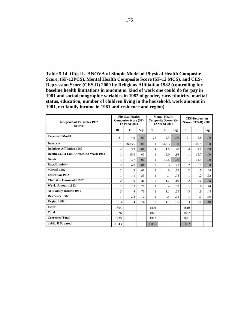
176
Table 5.14 Obj. II. ANOVA of Simple Model of Physical Health Composite Score, (SF-12PCS), Mental Health Composite Score (SF-12 MCS), and CES-Depression Score (CES-D) 2000 by Religious Affiliation 1982 (controlling for baseline health limitations in amount or kind of work one could do for pay in 1981 and sociodemographic variables in 1982 of gender, race/ethnicity, marital status, education, number of children living in the household, work amount in 1981, net family income in 1981 and residence and region).
Physical Health Composite Score (SF-
12 PCS) 2000
Mental Health Composite Score (SF-
12 MCS) 2000
CES-Depression Score (CES-D) 2000 Independent Variables 1982
Source Df F Sig. df F Sig. df F Sig.
Corrected Model 21 4.9 .00 21 2.5 .00 21 5.8 .00
Intercept 1 3435.5 .00 1 3568.5 .00 1 107.9 .00Religious Affiliation 1982 4 3.2 .01 4 1.5 .20 4 2.1 .08Health Could Limit Amt/Kind Work 1981 1 45.9 .00 1 2.0 .16 1 15.7 .00Gender 1 3.7 .06 1 19.4 .00 1 11.9 .00Race/Ethnicity 2 4.9 .01 2 .3 .73 2 5.5 .00Marital 1982 2 .5 .61 2 .5 .59 2 .5 .64Education 1982 1 1.1 .29 1 .1 .78 1 .2 .62Child # in Household 1982 2 .9 .41 2 1.7 .19 2 7.4 .00Work Amount 1982 1 1.3 .26 1 .4 .53 1 .6 .44Net Family Income 1981 3 .4 .76 3 1.1 .35 3 .9 .45Residence 1982 1 2.4 .12 1 .4 .54 1 .3 .56Region 1982 3 .4 .74 3 1.1 .36 3 2.1 .10Error 1804 1804 1810 Total 1826 1826 1832 Corrected Total 1825 1825 1831 a Adj. R Squared 0.043 0.017 .052

177
Table 5.15 Obj. II. Parameter Estimates of Simple Model of Physical Health Composite Score, (SF-12PCS), Mental Health Composite Score (SF-12 MCS), and CES-Depression Score (CES-D) 2000 by Religious Affiliation 1982 (controlling for baseline health limitations in amount or kind of work one could do for pay in 1981 and sociodemographic variables in 1982 of gender, race/ethnicity, marital status, education, number of children living in the household, work amount in 1981, net family income in 1981 and residence and region).
Physical Health Composite Score (SF-12 PCS) 2000
Mental Health Composite Score (SF-12 MCS) 2000
CES-Depression Score (CES-D) 2000 Independent
Variables 1982 Parameter B
Sig. CI 95% B Sig. CI
95% B Sig. CI
95%
Intercept 50.9 .00 48.22 53.57 53.7 .00 50.9 56.5 2.7 .00 1.3 4.1
Protestant 1982 1.9 .00 .63 3.12 1.4 .03 .1 2.8 -.7 .03 -1.4 -.1 Roman Catholic 1982 1.7 .02 .32 3.08 1.2 .09 -.2 2.7 -.6 .11 -1.3 .1
Jewish 1982 4.7 .02 .73 8.61 3.1 .14 -1.1 7.3 -2.5 .02 -4.5 -.4
Other 1982 3.3 .03 .25 6.30 .3 .88 -2.9 3.4 -.5 .55 -2.1 1.1
None 1982 0(a) . . . 0(a) . . . 0(a) . . . 1981 Hlh Limits Work Yes -5.9 .00 -7.62 -4.20 -1.3 .16 -3.1 .5 1.8 .00 .9 2.7
1981 Hlh Limits Work No 0(a) . . . 0(a) . . . 0(a) . . .
Female -.8 .06 -1.56 .02 -1.9 .00 -2.7 -1.0 .7 .00 .3 1.1
Male 0(a) . . . 0(a) . . . 0(a) . . .
Hispanic -1.3 .04 -2.46 -.08 .3 .66 -1.0 1.5 .3 .41 -.4 .9
African American -1.4 .01 -2.33 -.37 -.3 .57 -1.3 .7 .9 .00 .4 1.4 Caucasian and others 0(a) . . . 0(a) . . . 0(a) . . .
Marital Status: Div./Wid./Sep 82 -.6 .51 -2.21 1.10 -.4 .68 -2.1 1.4 -.2 .60 -1.1 .6
Married 1982 .3 .60 -.76 1.32 -.6 .31 -1.7 .5 -.3 .36 -.8 .3
Never Married 82 0(a) . . . 0(a) . . . 0(a) . . . Education Level: >=High School 82
1.1 .29 -.90 3.06 .3 .78 -1.8 2.4 -.3 .62 -1.3 .8
< High School 82 0(a) . . . 0(a) . . . 0(a) . . .
>=2 Children 82 -1.0 .18 -2.35 .44 -1.3 .09 -2.8 .2 1.3 .00 .6 2.1
1 Child 82 -.4 .52 -1.55 .78 -.1 .92 -1.3 1.2 .8 .01 .2 1.4
No Children 82 0(a) . . . 0(a) . . . 0(a) . . . Work Full-Time 81 .5 .26 -.40 1.49 -.3 .53 -1.3 .7 -.2 .44 -.7 .3
Work Part-Time 81 0(a) . . . 0(a) . . . 0(a) . . .
Income 81 Missing -.6 .31 -1.84 .59 -1.0 .15 -2.2 .3 .4 .23 -.2 1.0
Income 81 Top 25% -.4 .55 -1.58 .84 -1.1 .10 -2.3 .2 .5 .13 -.1 1.1
Income 81 Mid 50% -.2 .75 -1.17 .84 -.7 .23 -1.7 .4 .3 .22 -.2 .9
Income 81 Lowest 25% 0(a) . . . 0(a) . . . 0(a) . . .

178
Table 5.15. (Continued).
Physical Health Composite Score (SF-12 PCS) 2000
Mental Health Composite Score (SF-12 MCS) 2000
CES-Depression Score (CES-D) 2000 Independent
Variables 1982 Parameter B
Sig. CI 95% B Sig. CI
95% B Sig. CI
95%
Residence 82 Urban -.8 .12 -1.81 .21 .3 .54 -.7 1.4 -.2 .56 -.7 .4
Residence 1982 Rural 0(a) . . . 0(a) . . . 0(a) . . .
Region 82: West -.6 .37 -1.86 .69 -.2 .81 -1.5 1.2 .4 .21 -.2 1.1
South 1982 .0 .98 -1.12 1.15 -.5 .44 -1.7 .7 .8 .01 .2 1.4
North Central 82 -.2 .71 -1.39 .94 .5 .44 -.7 1.7 .4 .16 -.2 1.1
Northeast 1982 0(a) . . . 0(a) . . . 0(a) . . . a This parameter is set to zero because it is redundant.
NoneOtherJewishCatholicProtestant
Religious Affiliation 1982 5 categories
51.00
50.00
49.00
48.00
47.00
46.00
Estim
ated
Mar
gina
l Mea
ns
Estimated Marginal Means of Physical Health Composite Score (SF-12, PCS)2000
Figure 5.10 Obj. II. Simple Model of Physical Health Composite Score (SF-12PCS) 2000 by Religious Affiliation 1982 (controlling for baseline health limitations in amount or kind of work one could do for pay in 1981 and sociodemographic variables in 1982 of gender, race/ethnicity, marital status, education, number of children living in the household, work amount in 1981, net family income in 1981 and residence and region).

179
NoneOtherJewishCatholicProtestant
Religious Affiliation 1982 5 categories
54.00
53.00
52.00
51.00
Estim
ated
Mar
gina
l Mea
ns
Estimated Marginal Means of Mental Health Composite Score (SF-12, MCS)2000
Figure 5.11 Obj. II. Simple Model of Mental Health Composite Score (SF-12 MCS) 2000 by Religious Affiliation 1982 (controlling for baseline health limitations in amount or kind of work one could do for pay in 1981 and sociodemographic variables in 1982 of gender, race/ethnicity, marital status, education, number of children living in the household, work amount in 1981, net family income in 1981 and residence and region).

180
NoneOtherJewishCatholicProtestant
Religious Affiliation 1982 5 categories
5.50
5.00
4.50
4.00
3.50
3.00
2.50
Estim
ated
Mar
gina
l Mea
ns
Estimated Marginal Means of CES-Depression Score
Figure 5.12 Obj. II. Simple Model of CES-Depression Score (CES-D) 2000 by Religious Affiliation 1982 (controlling for baseline health limitations in amount or kind of work one could do for pay in 1981 and sociodemographic variables in 1982 of gender, race/ethnicity, marital status, education, number of children living in the household, work amount in 1981, net family income in 1981 and residence and region).

181
Objective II.4. The influence of change in religious attendance from 1982 to 2000 on
physical health, mental health, and depression in 2000, controlling for 1982
sociodemographic factors.
Results for Objective II.4: No change in moderate attendance of one to three times per
month from 1982 to 2000 was associated with better physical health and mental health
scores and with the lowest depression scores in mid-adulthood. The general trend was
that no change or constant attendance (ranging from more than once per week to
infrequent attendance) from 1982 to 2000 was associated with better health in 2000,
compared with those who change in attendance, with the exception of those who
decreased in attendance, who also reported better health.
Physical Health
The relationship between change in religious attendance from 1982 to 2000 and
physical health was overall significant (refer to ANOVA Table 5.16). However, the
various categories were not significantly different from the baseline (refer to
Parameter Estimate Table 5.17). The overall trend was that those with no change in
attendance from 1982 to 2000 reported better physical health scores in 2000, with the
highest score at no change in high attendance (>1/wk to 1/wk). Those with changes in
attendance over time had poorer physical health scores (refer to Figure 5.13). Other
factors related to poorer physical scores were having a health limitation in 1981, being
female, African American or Hispanic, and rural residence in 1982.
Mental Health
The relationship between change in religious attendance from 1982 to 2000 and
mental health was overall significant (refer to ANOVA Table 5.16). Figure 5.14 shows
that the best mental health scores occurred for those who had no change in moderate

182
attendance from 1982 to 2000 as well as those with a high decrease in attendance over
time. Those with the lowest reported scores were either associated with a high increase
in attendance over time or with no change in high attendance over time. Other factors
related to poorer mental health scores were having a health limitation in 1981 and
being female.
Depression
The relationship between change in religious attendance from 1982 to 2000 and
depression was overall significant (refer to ANOVA Table 5.16). Figure 5.15 shows
the lowest depression scores in 2000 for those with no change in moderate attendance.
Low depression scores were also reported for those with a decrease in attendance over
time. The highest depression score was found among those with the highest increase in
attendance from 1982 to 2000 (refer to Table 5.17).
The other factors related to lower levels of depression in 2000 included not having a
health limitation in 1981, being male, and no children (living with respondent) in
1982. Higher depression scores were associated with being African American, and
living in the South and North Central region of the United States.
Addition of 1998 Sociodemographic Control Variables, with the 1982
Sociodemographic Control Variables to the Model
In addition to the sociodemographic 1982 variables, 1998 sociodemographic variables
(listed in Table 5.4) were added to the above model, as controls. Similar associations
were found between change in religious attendance 1982 and each health outcome in
2000 controlling for 1982 sociodemographic factors only compared to controlling for
both 1982 and 1998 sociodemographic factors.

183
Table 5.16 Obj. II. ANOVA of Simple Model Simple Model of Physical Health Composite Score, (SF-12PCS), Mental Health Composite Score (SF-12 MCS), and CES-Depression Score (CES-D) 2000 by Change in Religious Attendance from 1982 to 2000 (controlling for baseline health limitations in amount or kind of work one could do for pay in 1981 and sociodemographic variables in 1982 of gender, race/ethnicity, marital status, education, number of children living in the household, work amount in 1981, net family income in 1981 and residence and region).
Physical Health Composite Score (SF-12 PCS) 2000
Mental Health Composite Score (SF-12 MCS) 2000
CES-Depression Score (CES-D) 2000 Independent Variables
1982 Source df F Sig. df F Sig. df F Sig.
Corrected Model 23 4.5 .00 23 3.0 .00 23 6.3 .00
Intercept 1 4627.5 .00 1 4957.6 .00 1 159.6 .00Change in Religious Attendance 1982 to 2000 6 2.2 .04 6 3.5 .00 6 5.0 .00
Health Could Limit Amt/Kind Work 1981 1 46.4 .00 1 2.8 .09 1 17.5 .00
Gender 1 5.2 .02 1 23.5 .00 1 16.8 .00Race/Ethnicity 2 7.4 .00 2 .8 .47 2 8.8 .00Marital 1982 2 .4 .67 2 .6 .54 2 .3 .77Education 1982 1 1.3 .26 1 .0 .91 1 .1 .75Child # in Household 1982 2 .7 .49 2 1.5 .23 2 6.4 .00
Work Amount 1982 1 1.1 .30 1 .4 .52 1 .5 .46Net Family Income 1981 3 .4 .78 3 1.0 .41 3 .7 .55Residence 1982 1 3.0 .09 1 .5 .48 1 .4 .53Region 1982 3 .6 .59 3 1.3 .27 3 3.4 .02Error 1802 1802 1808 Total 1826 1826 1832 Corrected Total 1825 1825 1831 a Adj. R Squared 0.043 0.024 0.062

184
Table 5.17 Obj. II. Parameter Estimates of Simple Model Simple Model of Physical Health Composite Score, (SF-12PCS), Mental Health Composite Score (SF-12 MCS), and CES-Depression Score (CES-D) 2000 by Change in Religious Attendance (RA) from 1982 to 2000 (controlling for baseline health limitations in amount or kind of work one could do for pay in 1981 and sociodemographic variables in 1982 of gender, race/ethnicity, marital status, education, number of children living in the household, work amount in 1981, net family income in 1981 and residence and region).
Physical Health Composite Score (SF-12 PCS) 2000
Mental Health Composite Score (SF-12 MCS) 2000
CES-Depression Score (CES-D) 2000 Independent
Variables 1982 Parameter B Sig. CI 95% B Sig. CI
95% B Sig CI
95%
Intercept 53.0 .00 50.1 55.8 56.8 .00 53.8 59.8 1.2 .12 -.3 2.7 Rel. Attend (RA) 1982 to 2000 High Increase
-.9 .27 -2.6 .7 -2.8 .00 -4.6 -1.0 1.5 .00 .6 2.3
Rel Attend982 to 2000 Low Increase
-.3 .75 -1.9 1.4 -1.3 .14 -3.0 .4 .5 .21 -.3 1.4
Rel Attend 1982 to 2000 No Change in High Attendance
1.1 .43 -1.6 3.7 -3.0 .04 -5.7 -.2 1.0 .15 -.4 2.4
RA 1982 to 2000 No Change in Moderate Attendance
.6 .54 -1.4 2.6 -.1 .96 -2.2 2.1 -.1 .92 -1.1 1.0
RA 1982 to 2000 No Change in Low Attendance
.9 .42 -1.3 3.0 -1.1 .32 -3.4 1.1 .3 .61 -.8 1.4
RA 1982 to 2000 Low Decrease in Attendance
.9 .28 -.7 2.6 -.7 .44 -2.5 1.1 .0 1.00 -.9 .9
RA 1982 to 2000 High Decrease in Attendance
0(a) . . . 0(a) . . . 0(a) . . .
81 Hlh Limits Work Yes -6.0 .00 -7.7 -4.3 -1.5 .09 -3.4 .3 1.9 .00 1.0 2.8
81 Hlh Limits Work No 0(a) . . . 0(a) . . . 0(a) . . .
Female -.9 .02 -1.7 -.1 -2.1 .00 -2.9 -1.2 .9 .00 .5 1.3
Male 0(a) . . . 0(a) . . . 0(a) . . .
Hispanic -1.6 .01 -2.7 -.4 .1 .91 -1.1 1.2 .5 .12 -.1 1.0
African American -1.7 .00 -2.6 -.7 -.6 .26 -1.6 .4 1.1 .00 .6 1.6 Caucasian and others 0(a) . . . 0(a) . . . 0(a) . . .
Marital Status: Div./Wid./Sep.1982 -.6 .45 -2.3 1.0 -.4 .67 -2.1 1.4 -.2 .64 -1.1 .7
Married 1982 .1 .81 -.9 1.2 -.6 .27 -1.7 .5 -.2 .51 -.7 .4 Never Married 1982 0(a) . . . 0(a) . . . 0(a) . . .
Education Level: >=High School 82 1.1 .26 -.9 3.1 .1 .91 -2.0 2.2 -.2 .75 -1.2 .9
< High School 82 0(a) . . . 0(a) . . . 0(a) . . .

185
Table 5.17 (Continued).
Physical Health Composite Score (SF-12 PCS) 2000
Mental Health Composite Score (SF-12 MCS) 2000
CES-Depression Score (CES-D) 2000 Independent
Variables 1982 Parameter B Sig. CI 95% B Sig. CI
95% B Sig CI
95%
>=2 Children 1982 -.9 .23 -2.3 .5 -1.1 .13 -2.6 .3 1.3 .00 .5 2.0
1 Child 1982 -.3 .63 -1.5 .9 .1 .89 -1.1 1.3 .8 .02 .1 1.4
No Children 1982 0(a) . . . 0(a) . . . 0(a) . . . Work Full-Time 81 .5 .30 -.4 1.4 -.3 .52 -1.3 .7 -.2 .46 -.7 .3
Work Part-Time 81 0(a) . . . 0(a) . . . 0(a) . . .
Income 81 Missing -.6 .34 -1.8 .6 -.9 .18 -2.2 .4 .3 .29 -.3 1.0 Income 81 Top 25% -.3 .57 -1.6 .9 -1.0 .12 -2.3 .3 .4 .18 -.2 1.1
Income 81 Mid 50% -.1 .83 -1.1 .9 -.6 .25 -1.7 .4 .3 .28 -.2 .8
Income 81 Lowest 25% 0(a) . . . 0(a) . . . 0(a) . . .
Work Part-Time 81 0(a) . . . 0(a) . . . 0(a) . . .
Residence 82 Urban -.9 .09 -1.9 .1 .4 .48 -.7 1.4 -.2 .53 -.7 .4
Residence 82 Rural 0(a) . . . 0(a) . . . 0(a) . . .
Region 82: West -.8 .22 -2.1 .5 -.3 .63 -1.7 1.0 .5 .12 -.1 1.2
South 82 -.2 .73 -1.3 .9 -.8 .21 -1.9 .4 1.0 .00 .4 1.5
North Central 82 -.5 .40 -1.7 .7 .2 .70 -1.0 1.5 .6 .04 .0 1.2
Northeast 82 0(a) . . . 0(a) . . . 0(a) . . . a This parameter is set to zero because it is redundant.

186
highdecrease inattend 82 to
2000(differenceof -3 or -4)
lowdecrease inattend 82 to
2000(differenceof -1 or -2)
no change inlow attend82 to 2000
(<=sev/yr ornot at all)
no change inmoderate
attend 82 to2000 (1-3
x/mth)
no change inhigh attend82 to 2000(>1/wk or
1/wk)
low increasein attend 82
to 2000(differenceof +1 or +2)
highincrease inattend 82 to
2000(differenceof +3 or +4)
Change in Religious Attendance 1982 to 2000 categories (based on 5levels)
49.00
48.50
48.00
47.50
47.00
46.50
Estim
ated
Mar
gina
l Mea
ns
Estimated Marginal Means of Physical Health Composite Score (SF-12, PCS)2000
Figure 5.13. Obj. II. Simple Model of Physical Health Composite Score (SF-12 PCS) 2000 by Change in Religious Attendance from 1982 to 2000 (controlling for baseline health limitations in amount or kind of work one could do for pay in 1981 and sociodemographic variables in 1982 of gender, race/ethnicity, marital status, education, number of children living in the household, work amount in 1981, net family income in 1981 and residence and region).

187
highdecrease inattend 82 to
2000(differenceof -3 or -4)
lowdecrease inattend 82 to
2000(differenceof -1 or -2)
no change inlow attend82 to 2000
(<=sev/yr ornot at all)
no change inmoderate
attend 82 to2000 (1-3
x/mth)
no change inhigh attend82 to 2000(>1/wk or
1/wk)
low increasein attend 82
to 2000(differenceof +1 or +2)
highincrease inattend 82 to
2000(differenceof +3 or +4)
Change in Religious Attendance 1982 to 2000 categories (based on 5levels)
53.00
52.00
51.00
50.00
Estim
ated
Mar
gina
l Mea
ns
Estimated Marginal Means of Mental Health Composite Score (SF-12, MCS)2000
Figure 5.14. Obj. II. Simple Model of Mental Health Composite Score (SF-12 MCS) 2000 by Change in Religious Attendance from 1982 to 2000 (controlling for baseline health limitations in amount or kind of work one could do for pay in 1981 and sociodemographic variables in 1982 of gender, race/ethnicity, marital status, education, number of children living in the household, work amount in 1981, net family income in 1981 and residence and region).

188
highdecrease inattend 82 to
2000(differenceof -3 or -4)
lowdecrease inattend 82 to
2000(differenceof -1 or -2)
no change inlow attend82 to 2000
(<=sev/yr ornot at all)
no change inmoderate
attend 82 to2000 (1-3
x/mth)
no change inhigh attend82 to 2000(>1/wk or
1/wk)
low increasein attend 82
to 2000(differenceof +1 or +2)
highincrease inattend 82 to
2000(differenceof +3 or +4)
Change in Religious Attendance 1982 to 2000 categories (based on 5 levels)
5.50
5.00
4.50
4.00
Estim
ated
Mar
gina
l Mea
ns
Estimated Marginal Means of CES-Depression Score
Figure 5.15 Obj. II. Simple Model of CES-Depression Score (CES-D) 2000 by Change in Religious Attendance from 1982 to 2000 (controlling for baseline health limitations in amount or kind of work one could do for pay in 1981 and sociodemographic variables in 1982 of gender, race/ethnicity, marital status, education, number of children living in the household, work amount in 1981, net family income in 1981 and residence and region).

189
Objective II.5. The effect of 1982 sociodemographic modifiers on the association
between change in religious attendance 1982 and physical health, mental health, and
depression 2000.
Results for Objective II.5. Change in religious attendance significantly interacted with
certain 1982 sociodemographic variables for each outcome of health (as described
below) in the presence of 1982 controls (at p<=0.10 for the ANOVA F test for overall
significance and for the individual Parameter Estimates). These same interactions were
still found to be significant in the presence of both sociodemographic 1982 and 1998
controls in each model.
Below I describe each of the one two-way interactions of change in religious
attendance with specific 1982 sociodemographic variables for each of the models with
physical health, mental health, or depression as the dependent variables. The
accompanying figures illustrating each interaction are listed after the text descriptions
of the interactions. These figures are presented rather than the ANOVA and parameter
estimate tables for simplicity of observing the effect of each interaction upon the
health outcome.
Physical Health: One Two-way Interactions of Health Limitations, Education,
Children, each with Change in Attendance from 1982 to 2000
For the model with the outcome variable of physical health, the sociodemographic
variables of health limitation in 1981, education in 1982, number of children in 1982,
and net family income in 1981 each interacted in one two-way interactions with the
change in religious attendance from 1982 to 2000 variable. In a two two-way
interaction, only health limitations and education were meaningfully significant.

190
One Two-Way Interaction: Health Limitation 1981 by Change in Attendance from
1982 to 2000
Those who reported that health could limit the amount or kind of work that they could
do for pay also varied in physical health score depending on the level of change in
religious attendance from 1982 to 2000. Those who reported a health limitation in
1981, and no change in low to moderate attendance, reported the best physical health
scores, while those with changes in attendance over time had lower scores. Among
those who reported no health limitations in 1981, physical health scores remained
fairly constant among the various levels of change in attendance (refer to Figure 5.16).
The ANOVA overall F test of the interaction was significant, but not the parameter
estimates (ANOVA F test = 1.918, p=0.075).
One Two-Way Interaction: Education 1982 by Change in Attendance from 1982 to
2000
Physical health scores did not vary across different levels of change in attendance
from 1982 to 2000 for those with some high school education or more. For those with
less than a high school education, however, physical health scores varied across
changes in attendance. Particularly for those with less than a high school education
and a high decrease in attendance from 1982 to 2000, physical health scores were
remarkably lower than all other levels (refer to Figure 5.17). Better physical health
scores for those with less than a high school education occurred for no change in
moderate attendance over time or a low decrease in attendance over time.

191
highdecrease inattend 82 to
2000(difference of
-3 or -4)
low decreasein attend 82 to
2000(difference of
-1 or -2)
no change inlow attend 82
to 2000(<=sev/yr or
not at all)
no change inmoderate
attend 82 to2000 (1-3
x/mth)
no change inhigh attend82 to 2000(>1/wk or
1/wk)
low increasein attend 82 to
2000(difference of
+1 or +2)
high increasein attend 82 to
2000(difference of
+3 or +4)
Change in Religious Attendance 1982 to 2000categories (based on 5 levels)
52.50
50.00
47.50
45.00
42.50
40.00
Estim
ated
Mar
gina
l Mea
ns
No (Hlh could not LimitAmt./Kind Work
Yes (Hlh could LimitAmt. or Kind Work)
Health Could Limit Kindor Amount Work for
Pay 81
Estimated Marginal Means of Physical Health Composite Score (SF-12, PCS)2000
Figure 5.16 Obj. II. Model of Physical Health Composite Score (SF-12 PCS) 2000 One Two-Way Interaction of Change in Religious Attendance 1982 to 2000 with Baseline Health Limitations in Amount or Kind of Work One Could Do for Pay in 1981 (controlling for baseline health limitations in amount or kind of work one could do for pay in 1981 and controlling for sociodemographic variables in 1982 of gender, race/ethnicity, marital status, education, number of children living in the household, work amount in 1981, net family income in 1981 and residence and region).

192
highdecrease inattend 82 to
2000(difference of
-3 or -4)
low decreasein attend 82 to
2000(difference of
-1 or -2)
no change inlow attend 82
to 2000(<=sev/yr or
not at all)
no change inmoderate
attend 82 to2000 (1-3
x/mth)
no change inhigh attend82 to 2000(>1/wk or
1/wk)
low increasein attend 82 to
2000(difference of
+1 or +2)
high increasein attend 82 to
2000(difference of
+3 or +4)
Change in Religious Attendance 1982 to 2000categories (based on 5 levels)
50.00
45.00
40.00
35.00Estim
ated
Mar
gina
l Mea
ns
< High School (grades0-8)
> High School (grades>=9)
Education 82 2categories
Estimated Marginal Means of Physical Health Composite Score (SF-12, PCS)2000
Figure 5.17 Obj. II. Model of Physical Health Composite Score (SF-12 PCS) 2000 One Two-Way Interaction of Change in Religious Attendance 1982 to 2000 with Education in 1982 (controlling for baseline health limitations in amount or kind of work one could do for pay in 1981 and controlling for sociodemographic variables in 1982 of gender, race/ethnicity, marital status, education, number of children living in the household, work amount in 1981, net family income in 1981 and residence and region).
One Two-Way Interaction: Children 1982 by Change in Attendance from 1982 to
2000
Physical health scores in 2000 remained fairly constant regardless of the change in
attendance levels among those not living with children in 1982. However, physical
health scores in 2000 fluctuated across changes in attendance levels for those with one
or more children in 1982. For those with two or more children, the best physical health
scores occurred at no change in moderate attendance and low decrease in attendance
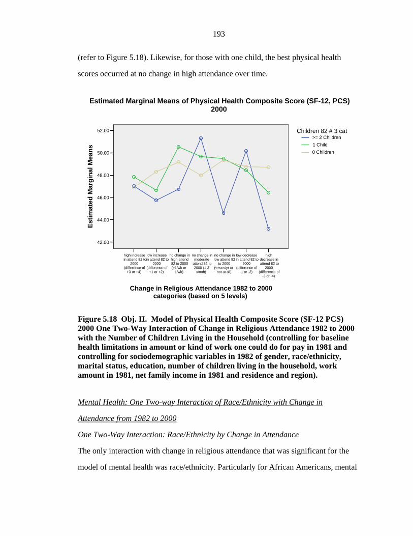
193
(refer to Figure 5.18). Likewise, for those with one child, the best physical health
scores occurred at no change in high attendance over time.
highdecrease inattend 82 to
2000(difference of
-3 or -4)
low decreasein attend 82 to
2000(difference of
-1 or -2)
no change inlow attend 82
to 2000(<=sev/yr or
not at all)
no change inmoderate
attend 82 to2000 (1-3
x/mth)
no change inhigh attend82 to 2000(>1/wk or
1/wk)
low increasein attend 82 to
2000(difference of
+1 or +2)
high increasein attend 82 to
2000(difference of
+3 or +4)
Change in Religious Attendance 1982 to 2000categories (based on 5 levels)
52.00
50.00
48.00
46.00
44.00
42.00
Estim
ated
Mar
gina
l Mea
ns 0 Children1 Child>= 2 Children
Children 82 # 3 cat
Estimated Marginal Means of Physical Health Composite Score (SF-12, PCS)2000
Figure 5.18 Obj. II. Model of Physical Health Composite Score (SF-12 PCS) 2000 One Two-Way Interaction of Change in Religious Attendance 1982 to 2000 with the Number of Children Living in the Household (controlling for baseline health limitations in amount or kind of work one could do for pay in 1981 and controlling for sociodemographic variables in 1982 of gender, race/ethnicity, marital status, education, number of children living in the household, work amount in 1981, net family income in 1981 and residence and region).
Mental Health: One Two-way Interaction of Race/Ethnicity with Change in
Attendance from 1982 to 2000
One Two-Way Interaction: Race/Ethnicity by Change in Attendance
The only interaction with change in religious attendance that was significant for the
model of mental health was race/ethnicity. Particularly for African Americans, mental

194
health scores fluctuated across the various levels of change in attendance. Among
African Americans, the lowest mental health score in 2000 occurred among those with
no change in high attendance from 1982 to 2000 (refer to Figure 5.19).
Figure 5.19 Obj. II. Model of Mental Health Composite Score (SF-12 MCS) 2000 One Two-Way Interaction of Change in Religious Attendance 1982 to 2000 with Race/Ethnicity (controlling for baseline health limitations in amount or kind of work one could do for pay in 1981 and controlling for sociodemographic variables in 1982 of gender, race/ethnicity, marital status, education, number of children living in the household, work amount in 1981, net family income in 1981 and residence and region).
highdecrease inattend 82 to
2000(difference of
-3 or -4)
low decreasein attend 82 to
2000(difference of
-1 or -2)
no change inlow attend 82
to 2000(<=sev/yr or
not at all)
no change inmoderate
attend 82 to2000 (1-3
x/mth)
no change inhigh attend82 to 2000(>1/wk or
1/wk)
low increase in attend 82 to
2000 (difference of
+1 or +2)
high increase in attend 82 to
2000 (difference of
+3 or +4)
Change in Religious Attendance 1982 to 2000 categories (based on 5 levels)
56.00
54.00
52.00
50.00
48.00
46.00
44.00
Estimated Marginal Means
Non-Black, Non-Caucasian and others
African American HispanicRace/Ethnicity
Estimated Marginal Means of Mental Health Composite Score (SF-12, MCS)2000

195
Depression: One Two-way Interaction Race/Ethnicity and Health Limitation 1981
each with Change in Attendance from 1982 to 2000
One Two-Way Interaction: Health Limitation 1981 by Change in Attendance
Those with health limitations varied in depression scores depending on the exhibited
level of change from 1982 to 2000. Among those who reported that health could limit
the kind or amount of work for pay they could do in 1981, those who reported no
change in high attendance reported the lowest depression scores, while those with a
high increase in attendance reported the highest depression scores (refer to Figure
5.20).
One Two-Way Interaction: Race/Ethnicity by Change in Attendance
For African Americans, there was a fluctuation in depression scores among the various
levels of change in attendance. Among African Americans, the highest depression
score occurred among those who reported no change in high attendance from 1982 to
2000 (refer to Figure 5.21).
One Two-Way Interaction: Child Number Living in the Household by Change in
Attendance
The highest depression scores were reported among those respondents living with two
or more children in a household and no change in high attendance from 1982 to 2000.
The remaining depression scores among those with one or no children fluctuated
mildly across the various change in attendance levels over time (refer to Figure 5.22).

196
highdecrease inattend 82 to
2000(difference of
-3 or -4)
low decreasein attend 82 to
2000(difference of
-1 or -2)
no change inlow attend 82
to 2000(<=sev/yr or
not at all)
no change inmoderate
attend 82 to2000 (1-3
x/mth)
no change inhigh attend82 to 2000(>1/wk or
1/wk)
low increasein attend 82 to
2000(difference of
+1 or +2)
high increasein attend 82 to
2000(difference of
+3 or +4)
Change in Religious Attendance 1982 to 2000categories (based on 5 levels)
10.00
8.00
6.00
4.00
2.00
0.00
Estim
ated
Mar
gina
l Mea
ns
No (Hlh could not LimitAmt./Kind Work
Yes (Hlh could LimitAmt. or Kind Work)
Health Could Limit Kindor Amount Work for
Pay 81
Estimated Marginal Means of CES-Depression Score
Figure 5.20 Obj. II. Model of CES-Depression Score (CES-D) 2000 One Two-Way Interaction of Change in Religious Attendance 1982 to 2000 with Baseline Health Limitations in Amount or Kind of Work One Could Do for Pay in 1981 (controlling for baseline health limitations in amount or kind of work one could do for pay in 1981 and controlling for sociodemographic variables in 1982 of gender, race/ethnicity, marital status, education, number of children living in the household, work amount in 1981, net family income in 1981 and residence and region).

197
Figure 5.21 Obj. II. Model of CES-Depression Score (CES-D) 2000 One Two-Way Interaction of Change in Religious Attendance 1982 to 2000 with Race/Ethnicity (controlling for baseline health limitations in amount or kind of work one could do for pay in 1981 and controlling for sociodemographic variables in 1982 of gender, race/ethnicity, marital status, education, number of children living in the household, work amount in 1981, net family income in 1981 and residence and region).
highdecrease inattend 82 to
2000(difference of
-3 or -4)
low decreasein attend 82 to
2000(difference of
-1 or -2)
no change inlow attend 82
to 2000(<=sev/yr or
not at all)
no change inmoderate
attend 82 to2000 (1-3
x/mth)
no change inhigh attend82 to 2000(>1/wk or
1/wk)
low increase in attend 82 to
2000 (difference of
+1 or +2)
high increase in attend 82 to
2000 (difference of
+3 or +4)
Change in Religious Attendance 1982 to 2000 categories (based on 5 levels)
10.00
8.00
6.00
4.00
2.00
Estimated Marginal Means Caucasian and others
African AmericanHispanicRace/Ethnicity
Estimated Marginal Means of CES-Depression Score

198
highdecrease inattend 82to 2000
(differenceof -3 or -4)
lowdecrease inattend 82to 2000
(differenceof -1 or -2)
no changein low
attend 82to 2000
(<=sev/yror not at
all)
no changein
moderateattend 82
to 2000 (1-3 x/mth)
no changein high
attend 82to 2000
(>1/wk or1/wk)
lowincrease inattend 82to 2000
(differenceof +1 or
+2)
highincrease inattend 82to 2000
(differenceof +3 or
+4)
Change in Religious Attendance 1982 to 2000categories (based on 5 levels)
9.00
8.00
7.00
6.00
5.00
4.00
3.00
2.00
Estim
ated
Mar
gina
l Mea
ns 0 Children1 Child>= 2 Children
Children 82 # 3 cat
Estimated Marginal Means of CES-Depression Score
Figure 5.22 Obj. II. Model of CES-Depression Score (CES-D) 2000 One Two-Way Interaction of Change in Religious Attendance 1982 to 2000 with the Number of Children Living in the Household (controlling for baseline health limitations in amount or kind of work one could do for pay in 1981 and controlling for sociodemographic variables in 1982 of gender, race/ethnicity, marital status, education, number of children living in the household, work amount in 1981, net family income in 1981 and residence and region).
Multicollinearity among the Religious Variables of Attendance, Change in Attendance
and Affiliation
Tests for multicollinearity and correlation revealed that the change in religious
attendance from 1982 to 2000 was collinear with the attendance 1982 variable
(Condition Index 15, correlation r = -0.7), as well as the affiliation variable (Condition
Index 11, correlation r = -0.7). Therefore, attendance 1982 and affiliation 1982 were
not included in the above models.

199
Relationship between Religious Attendance 1982 and Health 2000, controlling for
Change in Attendance 1982 to 2000
Models were explored to examine the influence of attendance, controlling for change
in attendance. Early adulthood attendance in 1982 was not significant, when
controlling for change in attendance 1982 to 2000, for any of the health outcomes.
Controlling for change in attendance from 1982 to 2000, attendance in 1982 was
significant only when it interacted with certain 1982 sociodemographic variables.
Because of the potential problem of multicollinearity and high correlation between
religious attendance and change in attendance, however, these results may not be
valid. Education 1982 and region 1982 modified the effect of religious attendance in
1982 on physical health in 2000. Race/Ethnicity, number of children in 1982 (and
region living in1982 [for the model with mental health as an outcome]) modified the
effects of religious attendance in 1982 on mental health and depression in 2000,
similar to the model (without controlling for change in attendance 1982 to 2000)
described in Objective II. In addition to 1982 sociodemographic factors, 1998
sociodemographic factors were added to this model. 1998 factors that modified the
influence of attendance in1982 on particular health outcomes in 2000 included work
amount in 1997 on physical health and net family income in 1997 on depression.
Conclusion: Summary of Objective II
Religious attendance in early adulthood was associated with better mental health and
less depression in mid-adulthood. This effect was modified by ethnicity and number of
children living in the household. Caucasians and those with no children who attended
more frequently reported better mental health scores and reported fewer depressive
symptoms compared to other ethnicities. In addition, they reported fewer depressive
symptoms than those living with two or more children in 1982.

200
Religious affiliation in young adulthood was associated with better physical health in
mid-adulthood. Those who identified with the Jewish faith in their early 20s reported
the best physical health scores and lowest depression scores, compared with those of
other affiliations. Those with no affiliation in their early 20s reported the lowest
physical health scores and highest depression scores in their early 40s, while those
who identified with a religious affiliation reported better health scores.
Generally, those who reported being consistent in their religious attendance,
particularly those showing no change in moderate attendance (one to three times per
month) from 1982 to 2000, reported better physical health, mental health, and
depression scores than those who reported changes in attendance. However, in some
instances a low decrease in attendance was associated with better health scores.
Discussion of Objective II
Strengths:
The strength of the study is the advantage of having a nationally representative sample
of young adults followed over a 20-year period from 1979 to 2000. The results benefit
from having two time points at which to measure religious attendance, in early
adulthood in 1982 and in later mid adulthood in 2000, making it possible to examine
the change in attendance over this eighteen-year period.
Limitations:
Study limitations include having few data points for religious attendance, with a large
gap of almost 20 years for which there was no attendance information. Although the
change in attendance from 1982 to 2000 can be measured, fluctuations in attendance
during this time cannot be measured. The dataset is also limited in having only one
point in time, in 2000, at which to measure health. The health module was added in

201
1998, and administered only once to each respondent, at the point of turning 40 or
over after 1998. Therefore, changes in health status along with changes in religious
attendance cannot be measured over time. There were few health variables available at
the beginning of the study to control for baseline health status, so the ability to control
for reverse causality was limited. The health variable available, “health could limit the
amount or kind of work for pay the respondent could do,” was somewhat crude.
The study was further limited by the restrictive range of the religious or spiritual
questions. Respondents were asked only about attendance and affiliation, the latter
limited almost entirely to the Judeo-Christian tradition. Spousal attendance and
affiliation were included, but since these questions were limited to those who reported
having been married, it excluded respondents from responding who were in non-
married domestic partnerships.
Those who increased in attendance from 1982 to 2000 reported having poorer physical
health, poorer mental health, and more depressive symptoms than those who remained
at the same level of attendance from 1982 to 2000. However, there was a potential
problem of reverse causality. It cannot be determined from the data whether poorer
health drives changes in attendance or changes in attendance produce poorer health.
The baseline health measure of 1981was crude. This baseline measures “whether
health could limit the kind or amount of work one could do for pay.”
For the interaction of change in attendance and health limitations, those who reported
a high increase in attendance or no change in moderate attendance also reported the
highest depression scores (refer to Figure 5.20). For physical health, those who

202
reported a health limitation in 1981, and reported a high increase in attendance from
1982 to 2000, also reported low physical health scores in 2000 (refer to Figure 5.16).
There was no intermediary health information available, during the period of 1982 to
2000, to determine whether changes in health were experienced during this almost 20-
year gap, in order to explain the changes in attendance.
However, it is clear from the data that associations between attendance and health can
be observed, as described above in the summary for Objective II.
Future Research Recommendations:
This study consistently showed that African Americans reported poorer mental health
and higher depression scores than Caucasians and Hispanics. Although more frequent
religious attendance during early adulthood was associated with better mental health
and lower depression scores among Caucasians, the opposite trend was observed for
African Americans, and more mildly so for Hispanics. It is unclear whether ethnicities
who attend more frequently in early adulthood are already in poorer mental health
before attending.
The findings that higher religious attendance levels for Caucasians during their early
20s (in 1982) is associated with better mental health and less depression in their early
40s (in 2000), yet attendance during their 40s (in 2000) is associated with poorer
mental health and more depression (in 2000), are interesting results which require
additional study to help elucidate these contradictory trends.
Another consistent finding in the various models run is that those living with two or
more children in 1982 reported fluctuating mental health and depression scores later in

203
life, depending on level of attendance in 1982, whereas those living with no children
in 1982 reported better mental health scores and lower depressive symptoms in 2000,
with increasing attendance. Because of lack of adequate measures of mental health and
depression prior to 1982 and during the eighteen years of the follow-up, it is unclear
whether those with more children were more depressed before 1982.
Another interesting, consistent finding in Objective II as well as in Objective I is that
those affiliated with the Jewish faith reported better physical health scores, controlling
for attendance and other sociodemographic variables. In a model with no control for
attendance, affiliation was significantly related to mental health and depression, with
those of the Jewish faith having the best health scores. Again, because of the low
frequency of those affiliated with the Jewish faith, the results may not be reliable.
However, it would be interesting in future studies to examine why this association
exists, and to test possible mediators to explain it.
Future survey rounds for this data may inquire of religious attendance again. It would
be interesting to conduct follow-up analyses, particularly if additional or subsequent
religious and health variables were included in later years among the same
respondents.
Policy Implications:
Epidemiology of religion is a relatively new field of study, gaining in prominence
rapidly over the last decade. It may therefore be premature to attempt to influence
policies on the basis of this research. More studies are needed if we are to establish
reliable associations among various forms of religious beliefs and practices, behaviors,
and physical and mental health outcomes.

204
Follow-up research on religious attendance, particularly on the differential effects of
race/ethnicity and number of children that might mediate the influence of religious
attendance on mental health and depression, is suggested.
This study provides some guideposts for examining this relationship, particularly
among differential effects that ethnicities, the number of children (or more generally
within the context of family dynamics), and religious affiliations may have on the
practice of attendance at religious services and their corresponding effects on health,
particularly mental health and depression.

205
CHAPTER 6 Objective III Results
Results for Objective III
Test for Mediation by Lifestyle and Behaviors of Alcohol Dependency (1994) and
Cigarette Smoking Frequency (1994) on The Relationship between Religious
Attendance (1982) in Early Adulthood and Physical Health, Mental Health, and
Depression in mid-Adulthood (2000)
Overview of Chapter
In this chapter I describe the results for Objective III as explained in Chapter 3 on
methods and objectives. Objective III is designed to test evidence of mediation of
lifestyle and behaviors, specifically alcohol use and cigarette smoking, to help explain
the relationship between religious attendance and each health variable. The other
objective is to test the effect of religious attendance during young adulthood on mid-
adulthood alcohol use and cigarette smoking. The chapter is organized as follows.
First, I describe the mediators of alcohol use and cigarette smoking. A brief summary
of the objectives and methods is presented, followed by a detailed description of the
results. The chapter concludes with a discussion of the strengths and limitations of the
study, related future research suggestions, and possible policy implications of the
results.
Descriptives of Behavior and Lifestyle Factors
The descriptives for the 1994 behavior and lifestyle factors for alcohol abuse and
dependency, frequency of heavy alcohol drinking, and cigarette smoking frequency
are cross-tabulated by religious attendance 1982, as listed in Table 6.1.

206
Table 6.1 Obj. III. Descriptives of Alcohol Abuse and Dependency 1994, Heavy Drinking 1994, and Cigarette Smoking 1994 by Religious Attendance in 1982 Unweighted.
Religious Attendance 1982 Variable
Row Totals
1.00 >1/wk 2.00 1/wk
3.00 1-3/mth
4.00 Infrequent (<=Sev./yr)
5.00 Not at all
Behaviors 1994
# Row % #
Row % #
Row % #
Row % #
Row % #
Var. Row Total
>= 1 symptom occur >= 1 time in last year
18 2.9 65 10.4 123 19.7 233 37.3 185 29.6 624 30.7
0 symptoms occur in last year
42 6.6 96 15.2 163 25.8 200 31.6 132 20.9 633 31.1
Alcohol Abuse or Dependency
NonDrinker (no alcohol in past mth or since last interview 1989)
75 9.7 135 17.4 180 23.2 212 27.3 174 22.4 776 38.2
>=1times in last month 17 3.0 57 10.0 118 20.7 199 34.9 180 31.5 571 29.0
0 times in last month (never) 37 5.9 95 15.2 152 24.4 213 34.1 127 20.4 624 31.7
Heavy Alcohol
Drinking Frequency Drink >=6 drinks on
one occasion
Nondrinkera 75 9.7 135 17.4 180 23.2 212 27.3 174 22.4 776 39.4
Cigarette Smoking Frequency
>=20 cig./day 11 3.7% 27 9.2% 44 15.0% 96 32.7% 116 39.5% 294 14.9%
<=19 cig./day 8 3.1% 27 10.5% 53 20.7% 98 38.3% 70 27.3% 256 13.0%
0 frequency (Nonsmokerb) 110 7.8% 232 16.4% 353 24.9% 428 30.2% 294 20.7% 1417 72.0%
Table Total 135 6.6% 296 14.6% 466 22.9% 645 31.7% 491 24.2% 2033 100%a Non-Smokers are defined as not smoking >=100 cigarettes in lifetime, or never smoked daily or not currently smoking or smoking occasionally. These individuals are treated as “valid skips” in the survey. b Non-Drinkers are defined as not drinking in last month or year. These individuals were treated as “valid skips” in the survey.

207
Alcohol Abuse or Dependency 1994 Descriptives
In 1994, approximately one-third of the cohort had experienced at least one symptom
of alcohol abuse or dependency at least once during the past year. Approximately one-
third had not experienced any symptoms, and the remaining were nondrinkers, defined
as not having had a drink either in the past month or since the last interview, 1989.
The nondrinkers were determined from valid skips for the alcohol-related questions.
Heavy Drinking 1994 Descriptives
Approximately one-third had experienced one or more episodes of heavy drinking in
the last month. Heavy drinking was defined as number of times in the past month of
having six or more drinks on one occasion. Approximately one-third had not
experienced any episodes of heavy drinking in the last month, and the remainder were
considered non-drinkers.
Cigarette Smoking Frequency 1994 Descriptives
Approximately one-third smoked cigarettes, approximately equally sub-divided
between those who smoked one or more packs per day and those who smoked less
than a pack per day. The remaining two-thirds were defined as non-smokers for the
purposes of this study. A nonsmoker was defined as having smoked less than 100
cigarettes in a lifetime, or having never smoked daily or not smoking currently or
smoking only occasionally. The nonsmokers were determined from being a valid skip
for the cigarette smoking frequency questions.
Those with one or more symptoms of alcohol abuse and dependency and of heavy
alcohol drinking in 1994 most commonly attended religious services infrequently in
1982, similar to those with no symptoms, and nondrinkers. Among heavy smokers in

208
1994, the highest frequency of attendance in 1982 was not at all, compared with
infrequent attendance for those who smoked less or not at all.
Weighted Descriptive Statistics for Alcohol Abuse or Dependency, Heavy Drinking
and Cigarette Smoking 1994
The 1994 unweighted descriptive statistics of alcohol abuse or dependency, heavy
drinking, and cigarette smoking were weighted using the year 2000 sample weight.
There were few differences in the unweighted compared to the weighted descriptives
statistics, all within a plus or minus 5 percent difference (compare Table 6.1 to Table
6.2 and Table 6.3). The size of the United States noninstitutionalized population of
which this study sample is representative was 9.0 million people in 1994 (refer to
Table 6.3).

209
Table 6.2 Obj. III. Descriptives of Alcohol Abuse or Dependency 1994, Heavy Drinking 1994, and Cigarette Smoking 1994 by Religious Attendance in 1982 Weighted (2000 sample weight divided by mean sample weight to obtain original sample size of approximately 2102 in order to directly compare frequency and percentage of each variable with the unweighted descriptive statistics) a, b
Behaviors 1994 Religious Attendance 1982
Variable Row Totals
1.00
>1/wk 2.00 1/wk 3.00 1-3/mth
4.00 Infrequent (<=Sev./yr)
5.00 Not at all
# Row % #
Row % #
Row % #
Row % #
Row % #
Var. Row Total
Alcohol Abuse or Dependency
>= 1 symptom occur >= 1 time in last year
17 2.5 58 8.6 127 19.0 264 39.4 204 30.4 670 32.9
0 symptoms occur in last year
44 6.5 95 14.3 154 23.1 217 32.5 157 23.5 668 32.8
NonDrinker (no Alcohol in past mth or since last interview 1989)
69 9.9 125 17.9 143 20.5 195 27.8 168 24.0 700 34.4
>=1times in last month 16 2.7 55 9.1 118 19.6 218 36.3 194 32.3 601 30.2
0 times in last month (never) 41 6.0 92 13.4 151 22.0 245 35.8 156 22.8 686 34.5
Heavy Alcohol
Drinking Frequency Drink >=6 drinks on
one occasion
Nondrinkerc 69 9.9 125 17.9 143 20.5 195 27.8 168 24.0 700 35.2
Cigarette Smoking Frequency
>=20 cig./day 13 3.6 30 8.3 53 14.6 110 30.4 157 43.1 363 18.3
<=19 cig./day 9 4.1 19 9.2 39 18.8 82 39.0 61 28.9 210 10.6
0 freq. (Nonsmokerd) 105 7.4 223 15.7 320 22.6 465 32.9 301 21.3 1413 71.2
Table Total 129 6.3 279 13.7 425 20.9 676 33.2 529 25.9 2038 100.0a The 2000 weight adjusts for loss to follow-up after the year 1979 in which the survey was administered through the year 2000. The sample 2000 weight adjusts for over-sampling of minorities, particularly Hispanics and African Americans. The weight also adjusts for two groups which were over-sampled and later dropped from the study. In 1985 an over-sample of approximately 1000 military personnel were dropped while 200 remained in the sample. In 1991 the over-sample of economically disadvantaged Caucasians was dropped from the study. The above descriptive statistics describe those individuals who were aged 40 and over in the year 2000, from a sample designed to be representative of noninstitutionalized people born between 1957 through 1964, living in the United States in 1978 (S. McClaskie, personal communication, Fall 2005). b The year 2000 sample weight is used for the descriptive statistics of the 1994 variables because the sample for the study is selected in the year 2000 (J. Zagorsky, personal communication, Fall 2005). c Non-Smokers are defined as not smoking >=100 cigarettes in lifetime, or never smoked daily or not currently smoking or smoking occasionally. These individuals are treated as “valid skips” in the survey. d Non-Drinkers are defined as not drinking in last month or year. These individuals were treated as “valid skips” in the survey.

210
Table 6.3 Obj. III. Descriptives of Alcohol Abuse or Dependency 1994, Heavy Drinking 1994, and Cigarette Smoking 1994 by Religious Attendance in 1982 Weighted (2000 sample weight used to obtain descriptive statistics of the noninstitutionalized U.S. population living in the U.S. in 1978 who were born between 1957 and 1964 and turned 40 and over in the year 2000).a, b
Religious Attendance 1982 Variable Row Totals
1.00 >1/wk 2.00 1/wk 3.00 1-3/mth 4.00 Infrequent
(<=Sev./yr) 5.00 Not at all Behaviors 1994
# Row % #
Row % #
Row % # Row % #
Row % #
Var. Row Total
>= 1 symptom occur >= 1 time in last year 73907 2.5 256956 8.6 565177 19.0 1171945 39.4 904054 30.4 2972039 32.9
0 symptoms occur in last year 193915 6.5 423651 14.3 685139 23.1 963074 32.5 696849 23.5 2962628 32.8
Alcohol Abuse or Dependency
NonDrinker (no Alcohol in past mth or since last interview 1989)
306266 9.9 555205 17.9 636306 20.5 864192 27.8 744437 24.0 3106406 34.4
>=1times in last month 71590 2.7 243835 9.1 523098 19.6 967345 36.3 860967 32.3 2666835 30.20 times in last month (never) 182480 6.0 409391 13.4 670524 22.0 1088845 35.8 692939 22.8 3044179 34.5
Heavy Alcohol Drinking Frequency Drink >=6 drinks on
one occasion Nondrinkerc
306266 9.9 555205 17.9 636306 20.5 864192 27.8 744437 24.0 3106406 35.2

211
Table 6.3 (Continued).
Behaviors 1994 Religious Attendance 1982 Variable Row Totals
1.00 >1/wk 2.00 1/wk 3.00 1-3/mth 4.00 Infrequent
(<=Sev./yr) 5.00 Not at all
# Row % # Row % #
Row % # Row % #
Row % #
Var. Row Total
0 times in last month (never) 182480 6.0 409391 13.4 670524 22.0 1088845 35.8 692939 22.8 3044179 34.5
Nondrinkera 306266 9.9 555205 17.9 636306 20.5 864192 27.8 744437 24.0 3106406 35.2
Cigarette Smoking Frequency
>=20 cig./day 57338 3.6 133488 8.3 235580 14.6 489570 30.4 695196 43.1 1611172 18.3
<=19 cig./day 38339 4.1 85588 9.2 175034 18.8 362534 39.0 268435 28.9 929929 10.6
0 freq. (Nonsmokerd) 464659 7.4 987460 15.7 1419314 22.6 2065073 32.9 1333297 21.3 6269803 71.2
Table Total 574088 6.3 1235812 13.7 1886621 20.9 2999211 33.2 2345340 25.9 9041073 100.0a The 2000 weight adjusts for loss to follow-up after the year 1979 in which the survey was administered through the year 2000. The sample 2000 weight adjusts for over-sampling of minorities, particularly Hispanics and African Americans. The weight also adjusts for two groups which were over-sampled and later dropped from the study. In 1985 an over-sample of approximately 1000 military personnel were dropped while 200 remained in the sample. In 1991 the over-sample of economically disadvantaged Caucasians was dropped from the study. The above descriptive statistics describe those individuals who were aged 40 and over in the year 2000, from a sample designed to be representative of noninstitutionalized people born between 1957 through 1964, living in the United States in 1978 (S. McClaskie, personal communication, Fall 2005). b The year 2000 sample weight is used for the descriptive statistics of the 1994 variables because the sample for the study is selected in the year 2000 (J. Zagorsky, personal communication, Fall 2005). c Non-Smokers are defined as not smoking >=100 cigarettes in lifetime, or never smoked daily or not currently smoking or smoking occasionally. These individuals are treated as “valid skips” in the survey. d Non-Drinkers are defined as not drinking in last month or year. These individuals were treated as “valid skips” in the survey.

212
Mediators of alcohol abuse or dependency, heavy alcohol drinking, and frequency
of cigarette smoking of the relationship between young adulthood religious
attendance and mid-adulthood physical health, mental health, and depression
Objective III.1. Determine whether 1994 lifestyle and behaviors of (1) alcohol abuse
or dependency, (2) frequency of heavy alcohol drinking, and (3) cigarette smoking
frequency mediate the relationship between religious attendance in young adulthood in
1982 to physical health, mental health, and depression in 2000.
Methods for Objective III.1.: Tests for mediation of lifestyle and behaviors,
particularly alcohol abuse or dependency, heavy alcohol drinking, and cigarette
smoking frequency in1994 were performed on the simple model of religious
attendance in1982 on the dependent health variables of physical health, mental health,
and depression in 2000, controlling for 1982 sociodemographic variables. An
explanation of the tests for mediation is described in greater detail in Chapter 3.
Results for Objective III.1
Depression
Alcohol abuse or dependency in 1994 and alcohol drinking in 1994 were each partial
mediators (although alcohol drinking showed evidence only as a very mild mediator)
on the effect of religious attendance in early adulthood, in 1982, on depression in mid-
adulthood, in 2000. Cigarette smoking frequency in 1994 mediated almost completely
the effect of religious attendance in early adulthood in 1982 on depression in mid-
adulthood, in 2000 (refer to Table 6.4 and Table 6.5).

213
In a simple model (without the presence of mediators), religious attendance in 1982
was significantly related to lower depression scores in 2000, controlling for other 1982
sociodemographic variables, as demonstrated in Chapter 5. In the presence of the
mediator of alcohol abuse or dependency, however, the effect of religious attendance
on depression became less significant overall, and less significant at most of the
individual levels of religious attendance. Likewise, alcohol abuse or dependency and
heavy alcohol drinking were related to higher depression scores (refer to Table 6.4,
Table 6.5, Figure 6.1, and Figure 6.2).
It should be noted that although the variable of heavy alcohol drinking was significant
overall in the model (ANOVA F test = 6.6, p=0.001), only the level of heavy drinking
at 0 frequency showed a result that was significantly different from that of the
nondrinkers (B= -0.6, p = 0.015). Therefore, it appears that within the heavy alcohol
drinking variable, only the level of alcohol drinking (defined at heavy drinking at 0
frequency) acts as a mediator, not the level of heavy alcohol drinking.
In summary, the mediators of alcohol abuse or dependency and alcohol drinking
explain some of the variance in depression 2000 scores, which were previously
attributed to religious attendance 1982 in the simple model (without the presence of
the mediators).
In the presence of the mediator of cigarette smoking in 1994, the effect of the various
levels of religious attendance in 1982 on depression in 2000 was borderline or no
longer significant. Heavy cigarette smoking in 1994 was significantly related to higher
depression scores in 2000 (Figure 6.3). The unique variance in depression scores in
2000, which religious attendance in 1982 previously explained in the simple model (in
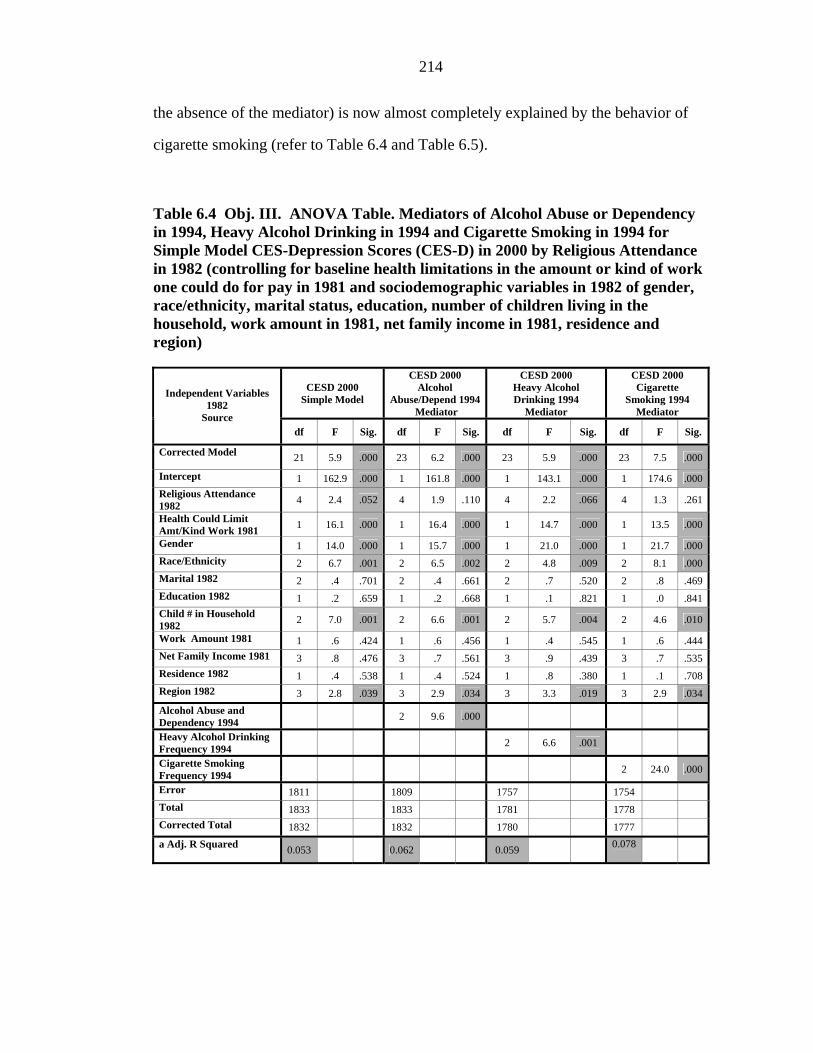
214
the absence of the mediator) is now almost completely explained by the behavior of
cigarette smoking (refer to Table 6.4 and Table 6.5).
Table 6.4 Obj. III. ANOVA Table. Mediators of Alcohol Abuse or Dependency in 1994, Heavy Alcohol Drinking in 1994 and Cigarette Smoking in 1994 for Simple Model CES-Depression Scores (CES-D) in 2000 by Religious Attendance in 1982 (controlling for baseline health limitations in the amount or kind of work one could do for pay in 1981 and sociodemographic variables in 1982 of gender, race/ethnicity, marital status, education, number of children living in the household, work amount in 1981, net family income in 1981, residence and region)
CESD 2000 Simple Model
CESD 2000 Alcohol
Abuse/Depend 1994 Mediator
CESD 2000 Heavy Alcohol Drinking 1994
Mediator
CESD 2000 Cigarette
Smoking 1994 Mediator
Independent Variables 1982
Source df F Sig. df F Sig. df F Sig. df F Sig.
Corrected Model 21 5.9 .000 23 6.2 .000 23 5.9 .000 23 7.5 .000
Intercept 1 162.9 .000 1 161.8 .000 1 143.1 .000 1 174.6 .000Religious Attendance 1982 4 2.4 .052 4 1.9 .110 4 2.2 .066 4 1.3 .261
Health Could Limit Amt/Kind Work 1981 1 16.1 .000 1 16.4 .000 1 14.7 .000 1 13.5 .000
Gender 1 14.0 .000 1 15.7 .000 1 21.0 .000 1 21.7 .000Race/Ethnicity 2 6.7 .001 2 6.5 .002 2 4.8 .009 2 8.1 .000Marital 1982 2 .4 .701 2 .4 .661 2 .7 .520 2 .8 .469Education 1982 1 .2 .659 1 .2 .668 1 .1 .821 1 .0 .841Child # in Household 1982 2 7.0 .001 2 6.6 .001 2 5.7 .004 2 4.6 .010
Work Amount 1981 1 .6 .424 1 .6 .456 1 .4 .545 1 .6 .444Net Family Income 1981 3 .8 .476 3 .7 .561 3 .9 .439 3 .7 .535Residence 1982 1 .4 .538 1 .4 .524 1 .8 .380 1 .1 .708Region 1982 3 2.8 .039 3 2.9 .034 3 3.3 .019 3 2.9 .034Alcohol Abuse and Dependency 1994 2 9.6 .000
Heavy Alcohol Drinking Frequency 1994 2 6.6 .001
Cigarette Smoking Frequency 1994 2 24.0 .000
Error 1811 1809 1757 1754 Total 1833 1833 1781 1778 Corrected Total 1832 1832 1780 1777 a Adj. R Squared 0.053 0.062 0.059 0.078

215
Mental Health
The only significant partial mediator for the relationship between attendance in 1982
and mental health scores in 2000 was cigarette smoking frequency. Alcohol abuse or
dependency and heavy alcohol drinking did not reveal evidence of mediation in the
relationship between religious attendance in 1982 and mental health scores in 2000. In
the simple model (without the presence of the mediator), religious attendance 1982
was significantly related to better mental health scores in 2000 (ANOVA F test = 2.86,
p=0.022; refer to Table 6.4), controlling for other sociodemographic variables. For
example, at attendance levels ranging from more than once per week to infrequent,
mental health scores improved (B = 2.2 to 1.4, p<0.05). When the mediator of
cigarette smoking frequency in 1994 was added to the model, the overall significance
of religious attendance lessened (ANOVA F test = 2.56, p=0.037), and each individual
level of religious attendance in 1982 became less significant. Heavy cigarette smoking
frequency was significantly related to lower mental health scores in the model (overall
significance: ANOVA F test = 7.52, p=0.001, and the individual level of heavy
cigarette smoking was significant at B = -2.2, p=0.00; refer to Figure 6.4.
Physical Health
There was no evidence of mediation for any of the potential mediators of alcohol
abuse or dependency, heavy alcohol drinking, or cigarette smoking frequency for the
relationship between religious attendance 1982 and physical health 2000.

216
Table 6.5 Obj. III. Parameter Estimate Table. Mediators of Alcohol Abuse or Dependency in 1994, Heavy Alcohol Drinking in 1994 and Cigarette Smoking Frequency in 1994 for the Simple Model of CES-Depression Scores (CES-D) in 2000 by Religious Attendance in 1982 (controlling for baseline health limitations in the amount or kind of work one could do for pay in 1981, and controlling for sociodemographic variables in 1982 of gender, race/ethnicity, marital status, education, number of children living in the household, work amount in 1981, net family income in 1981, residence and region)
CESD 2000 Simple Model
CESD 2000 Simple Model 1982 with Alcohol Abuse/Depend 1994
Mediator
CESD 2000 Simple Model 1982 with Heavy Alcohol Drinking 1994
Mediator
CESD 2000 Simple Model 1982 with Cigarette
Smoking 1994 Mediator Independent Variables 1982 Parameter B Sig CI 95% B Sig CI 95% B Sig. CI 95% B Sig. CI 95%
Intercept 2.4 .000 1.1 3.7 2.4 .000 1.1 3.8 2.3 .001 .9 3.6 1.7 .011 .4 3.0 Rel. Attend.(RA) 1982 >1/wk -1.1 .012 -2.0 -.2 -1.0 .025 -1.8 -.1 -1.0 .027 -1.9 -.1 -.7 .095 -1.6 .1
RA 1982 1/wk -.6 .083 -1.2 .1 -.5 .138 -1.1 .2 -.5 .116 -1.2 .1 -.3 .334 -1.0 .3
RA 1982 1-3x/mth -.7 .015 -1.3 -.1 -.6 .032 -1.2 -.1 -.8 .010 -1.4 -.2 -.6 .049 -1.2 .0 RA 1982<=Sev.x/yr (Infreq.) -.5 .050 -1.1 .0 -.5 .057 -1.0 .0 -.5 .053 -1.1 .0 -.4 .104 -1.0 .1
RA 1982 Not at all (No) 0(a) . . . 0(a) . . . 0(a) . . . 0(a) . . .
1981 Hlh Limits Amt./Kind Work Yes
1.8 .000 .9 2.7 1.8 .000 1.0 2.7 1.8 .000 .9 2.6 1.7 .000 .8 2.6
1981 Hlh Limits Amt/Kind Work No 0(a) . . . 0(a) . . . 0(a) . . . 0(a) . . .
Female .8 .000 .4 1.2 .9 .000 .4 1.3 1.0 .000 .6 1.5 1.0 .000 .6 1.4
Male 0(a) . . . 0(a) . . . 0(a) . . . 0(a) . . .
Hispanic .4 .222 -.2 1.0 .4 .234 -.2 .9 .3 .348 -.3 .9 .6 .061 .0 1.2
African American .9 .000 .4 1.4 .9 .000 .4 1.4 .8 .002 .3 1.3 1.0 .000 .5 1.5 Caucasian and Others 0(a) . . . 0(a) . . . 0(a) . . . 0(a) . . .
Marital Status: Div./Wid./Sep.1982 -.2 .606 -1.1 .6 -.2 .689 -1.0 .7 -.1 .760 -1.0 .7 -.3 .541 -1.1 .6
Married 1982 -.2 .431 -.8 .3 -.2 .369 -.8 .3 -.3 .253 -.9 .2 -.3 .231 -.9 .2
Never Married 1982 0(a) . . . 0(a) . . . 0(a) . . . 0(a) . . .

217
Table 6.5 (Continued).
CESD 2000 Simple Model
CESD 2000 Simple Model 1982 with Alcohol Abuse/Depend 1994
Mediator
CESD 2000 Simple Model 1982 with Heavy Alcohol Drinking 1994
Mediator
CESD 2000 Simple Model 1982 with Cigarette
Smoking 1994 Mediator Independent Variables 1982 Parameter B Sig CI 95% B Sig CI 95% B Sig. CI 95% B Sig. CI 95% Education Level: >=High School 1982 -.2 .659 -1.3 .8 -.2 .668 -1.3 .8 -.1 .821 -1.2 .9 -.1 .841 -1.2 .9
< High School 1982 0(a) . . . 0(a) . . . 0(a) . . . 0(a) . . .
>=2 Children 1982 1.3 .000 .6 2.1 1.3 .001 .5 2.0 1.2 .001 .5 1.9 1.1 .003 .4 1.9
1 Child 1982 .8 .012 .2 1.4 .8 .015 .2 1.4 .7 .027 .1 1.3 .5 .098 -.1 1.1
No Children 1982 0(a) . . . 0(a) . . . 0(a) . . . 0(a) . . .
Work Full-Time 1981 -.2 .424 -.7 .3 -.2 .456 -.7 .3 -.2 .545 -.7 .3 -.2 .444 -.7 .3
Work Part-Time 1981 0(a) . . . 0(a) . . . 0(a) . . . 0(a) . . .
Income 1981 Missing .4 .234 -.3 1.0 .3 .296 -.3 1.0 .4 .181 -.2 1.1 .4 .222 -.2 1.0 Income 1981 Top 25% .5 .148 -.2 1.1 .4 .185 -.2 1.1 .5 .162 -.2 1.1 .4 .203 -.2 1.1
Income 1981 Mid 50% .3 .240 -.2 .8 .3 .280 -.2 .8 .4 .189 -.2 .9 .3 .267 -.2 .8
Income 1981 Lowest 25% 0(a) . . . 0(a) . . . 0(a) . . . 0(a) . . .
Residence 1982 Urban -.2 .538 -.7 .4 -.2 .524 -.7 .4 -.2 .380 -.8 .3 -.1 .708 -.6 .4
Residence 1982 Rural 0(a) . . . 0(a) . . . 0(a) . . . 0(a) . . .
Region 1982: West .5 .130 -.2 1.2 .5 .128 -.1 1.2 .6 .083 -.1 1.3 .6 .076 -.1 1.3
South 1982 .9 .004 .3 1.5 .9 .003 .3 1.5 1.0 .002 .4 1.5 .9 .003 .3 1.5
North Central 1982 .6 .069 .0 1.2 .5 .075 -.1 1.2 .6 .060 .0 1.2 .6 .069 .0 1.2
Northeast 1982 0(a) . . . 0(a) . . . 0(a) . . . 0(a) . . .

218
Table 6.5 (Continued).
CESD 2000 Simple Model
CESD 2000 Simple Model 1982 with Alcohol Abuse/Depend 1994
Mediator
CESD 2000 Simple Model 1982 with Heavy Alcohol Drinking 1994
Mediator
CESD 2000 Simple Model 1982 with Cigarette
Smoking 1994 Mediator Independent Variables 1994 Parameter B Sig CI 95% B Sig CI 95% B Sig. CI 95% B Sig. CI 95% Alcohol 1994 Abuse/Depend >=1 Symptom in past year
.4 .085 -.1 .9
No Symptoms in past year 1994 -.7 .007 -1.1 -.2
NonDrinker 1994 0(a) . . . Heavy Alcohol 1994 Drinking >=1/mth .3 .185 -.2 .9
Heavy Alcohol 1994 Drinking 0/mth (never)
-.6 .015 -1.1 -.1
NonDrinker (valid skip) 1994 0(a) . . .
Cig. Smoking 1994 >=1 pack/day 2.0 .000 1.4 2.6
Cig. Smoking 1994 < pack/day .5 .080 -.1 1.1
NonSmoker 1994 0(a) . . . a This parameter is set to zero because it is redundant.

219
No Alcohol in past 30 days orsince last interview 1989 day
No Alcohol Abuse/Dependsymptoms occur in past yr.
>=1 Alcohol Abuse/Dependencysymptoms occur >=1 in past yr
Alcohol Dependency or Abuse Symptoms based on Behavior and Lifestylesymptoms (categorical)
5.20
5.00
4.80
4.60
4.40
4.20
4.00
Estim
ated
Mar
gina
l Mea
ns
Estimated Marginal Means of CES-Depression Score
Figure 6.1 Obj. III. Mediator of Alcohol Abuse or Dependency in 1994, for the Simple Model of CES-Depression Scores (CES-D) in 2000 by Religious Attendance in 1982 (controlling for baseline health limitations in the amount or kind of work one could do for pay in 1981, and sociodemographic variables in 1982 of gender, race/ethnicity, marital status, education, number of children living in the household, work amount in 1981, net family income in 1981, residence and region).

220
NonDrinker (valid skip)0 times (never)>= 1 times
Drinks 6 or more on one occasion frequency
5.00
4.80
4.60
4.40
4.20
4.00
3.80
Estim
ated
Mar
gina
l Mea
ns
Estimated Marginal Means of CES-Depression Score
Figure 6.2 Obj. III. Mediator of Heavy Alcohol Drinking in 1994, for the Simple Model of CES-Depression Scores (CES-D) in 2000 by Religious Attendance in 1982 (controlling for baseline health limitations in the amount or kind of work one could do for pay in 1981, and sociodemographic variables in 1982 of gender, race/ethnicity, marital status, education, number of children living in the household, work amount in 1981, net family income in 1981, residence and region).

221
0 freq. for smoker or valid skip(nonsmoker)
<=19 cig./day>=20 cig./day
Cigarette Frequency 1994
6.50
6.00
5.50
5.00
4.50
4.00
Estim
ated
Mar
gina
l Mea
ns
Estimated Marginal Means of CES-Depression Score
Figure 6.3 Obj. III. Mediator of Cigarette Smoking Frequency in 1994, for the Simple Model of CES-Depression Scores (CES-D) in 2000 by Religious Attendance in 1982 (controlling for baseline health limitations in the amount or kind of work one could do for pay in 1981, and sociodemographic variables in 1982 of gender, race/ethnicity, marital status, education, number of children living in the household, work amount in 1981, net family income in 1981, residence and region).
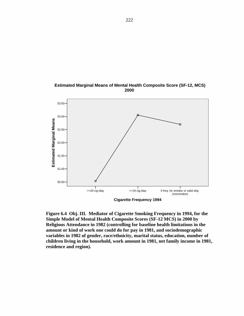
222
0 freq. for smoker or valid skip(nonsmoker)
<=19 cig./day>=20 cig./day
Cigarette Frequency 1994
53.50
53.00
52.50
52.00
51.50
51.00
50.50
Estim
ated
Mar
gina
l Mea
ns
Estimated Marginal Means of Mental Health Composite Score (SF-12, MCS)2000
Figure 6.4 Obj. III. Mediator of Cigarette Smoking Frequency in 1994, for the Simple Model of Mental Health Composite Scores (SF-12 MCS) in 2000 by Religious Attendance in 1982 (controlling for baseline health limitations in the amount or kind of work one could do for pay in 1981, and sociodemographic variables in 1982 of gender, race/ethnicity, marital status, education, number of children living in the household, work amount in 1981, net family income in 1981, residence and region).

223
The Effects of Religious Attendance on later Alcohol Abuse or Dependency, Heavy
Alcohol Drinking, and Cigarette Smoking Frequency
Objective III.2. Determine whether religious attendance in young adulthood 1982 is
protective against (1) alcohol abuse or dependency, (2) heavy alcohol drinking, and
(3) cigarette smoking frequency, twelve years later in mid-adulthood, 1994,
controlling for other sociodemographic characteristics.
Methods for Objective III.2
Separate multinomial logistic regression models were performed for each of the
dependent variables in 1994 of (1) alcohol abuse or dependency, (2) heavy alcohol
drinking frequency and, (3) cigarette smoking frequency, by the dependent variable of
religious attendance in1982, controlling for baseline health limitations in 1981 and
1982 sociodemographic characteristics (gender, race/ethnicity, marital status,
education, work amount in 1981, net family income in 1981, residence and region).
Results for Objective III.2
The Effects of Religious Attendance on Alcohol Abuse or Dependency
Frequent religious attendance of more than once per week to once per week in young
adulthood was found to be protective against alcohol abuse or dependency, controlling
for sociodemographic variables in 1982 of gender, race/ethnicity, marital status,
education, work amount, net family income, residence and region (refer to Likelihood
Ratio Test, Table 6.6, and the Multinomial logistic regression, Table 6.7). For
example, those who reported attending more than once a week in young adulthood had
a 70 percent lower odds of being an alcohol abuser twelve years later, compared with
those who did not report attending as young adults (OR = 0.29 [0.16,0.53] 95% CI;
refer to Table 6.7), while those who reported attending once per week had a 45 percent

224
lower odds of being an alcohol abuser or dependent twelve years later than
nonattenders (OR = 0.55 [0.37, 0.82] 95%CI; refer to Table 6.7). Moderate attendance
of one to three times per month was found to be borderline protective (p=0.064; refer
to Table 6.7). Infrequent attendance was not protective.
Other protective factors against alcohol abuse or dependency at young adulthood
included being female, Hispanic or African American, working less than twenty hours
per week, and rural residence (refer to Table 6.7).
Predictive factors in young adulthood for being a nondrinker twelve years later
included being female, Hispanic or African American, married, working less than
twenty hours per week, and rural residence (refer to Table 6.8).
The Effects of Religious Attendance on Frequency of Heavy Alcohol Drinking
Frequent to moderate attendance in young adulthood was protective against heavy
alcohol drinking twelve years later, in mid-adulthood, controlling for 1982
sociodemographic variables of gender, race/ethnicity, marital status, education, work
amount, net family income, residence and region (refer to the Log likelihood ratio test,
Table 6.6, and the Multinomial logistic regression, Table 6.8). A young adult who
attended religious services more than once per week to once per month had a 70 to 40
percent lower odds of being a heavy alcohol drinker twelve years later (OR = 0.27
[0.14, 0.50] 95%CI; OR=0.69 [0.48, 0.98] 95%CI; refer to Table 6.8).
Religious attendance of more than once per week to moderate attendance of one to
three times per month as a young adult had no affect on whether a person drank
alcohol later in adulthood; although infrequent attendance was predictive of later
alcohol use (OR=1.42 (1.03, 1.97) 95%CI; refer to Table 6.8).

225
Other protective factors in young adulthood against heavy alcohol use later in
adulthood were being female, Hispanic or African American, working less than twenty
hours per week, and rural residence (refer to Table 6.8). Predictive factors in young
adulthood of being a nondrinker twelve years later were being African American or
Hispanic, married, and a rural residence.
Predictive factors for using alcohol twelve years later were having a higher education
level of some high school or more (OR =3.70[1.50, 9.07] 95%CI), and working twenty
or more hours per week (OR=1.45[1.09, 1.94] 95%CI; refer toTable 6.8).
The Effects of Religious Attendance on Frequency of Cigarette Smoking
Any amount of religious attendance in young adulthood was protective against heavy
cigarette use twelve years later (refer to Log likelihood ratio test, Table 6.6, and the
Multinomial logistic regression, Table 6.9). Increasing religious attendance provided
increasing protection against heavy cigarette use. Young adults who attended more
than once per week had about a 75 percent lower odds of heavy smoking twelve years
later compared with nonattenders (OR=0.24 [0.11, 0.50] 95%CI; refer to Table 6.9).
Young adults who attended infrequently had a 40 percent lower odds of heavy
smoking twelve years later (OR=0.60 [0.43, 0.84] 95%CI; refer to Table 6.9).
Other protective factors during young adulthood against heavy cigarette smoking in
later adulthood were being female, African American or Hispanic, never married, not
living with children in the household, and rural residence (refer to Table 6.9).
Frequent-to-moderate religious attendance in young adulthood was protective against
smoking twelve years later (refer to Table 6.9). Infrequent attendance did not protect
against smoking.

226
Other protective factors against smoking twelve years later were being Caucasian, and
not living with children in the household in young adulthood (refer to Table 6.9).
Table 6.6 Obj. III. Multinomial Logistic Regression, Likelihood Ratio Tests. Alcohol Abuse and Dependency 1994, Heavy Alcohol Drinking 1994 and Cigarette Smoking 1994 as Dependent Variables in the Simple Model of Religious Attendance in 1982 (controlling for baseline health limitations in the amount or kind of work one could do for pay in 1981, and sociodemographic variables in 1982 of gender, race/ethnicity, marital status, education, number of children living in the household, work amount in 1981, net family income in 1981, residence and region).
Alcohol Abuse/Depend 1994 Dependent Variable
Heavy Alcohol Drinking 1994
Dependent Variable
Cigarette Smoking 1994
Dependent Variable Independent Variables 1982 Source
X2 df Sig. X2 df Sig. X2 df Sig.
Final Model 215.7 42 .000 299.4 42 .000 208.2 42 .000
Intercept .0 a 0 . .0 a 0 . .0 a 0 . Religious Attendance 1982 44.1 8 .000 42.6 8 .000 60.7 8 .000Health Could Limit Amt/Kind Work 1981 .0 2 .984 .3 2 .880 3.2 2 .199
Gender 54.9 2 .000 113.8 2 .000 12.2 2 .002Race/Ethnicity 20.0 4 .000 24.0 4 .000 55.1 4 .000Marital 1982 7.4 4 .116 7.2 4 .125 8.0 4 .093Education 1982 1.7 2 .438 11.3 2 .004 1.3 2 .535Child # in Household 1982 2.2 4 .695 7.1 4 .130 20.8 4 .000Work Amount 1981 10.5 2 .005 8.5 2 .014 1.5 2 .463Net Family Income 1981 4.0 6 .679 3.0 6 .813 3.3 6 .768Residence 1982 19.4 2 .000 20.5 2 .000 5.2 2 .075Region 1982 3.9 6 .687 5.2 6 .520 3.9 6 .685Pseudo R sqr. Cox and Snell 0.111 0.154 0.110
a The chi-square statistic is the difference in -2 log-likelihoods between the final model and a reduced model. The reduced model is formed by omitting an effect from the final model. The null hypothesis is that all parameters of that effect are 0. This reduced model is equivalent to the final model because omitting the effect does not increase the degrees of freedom.
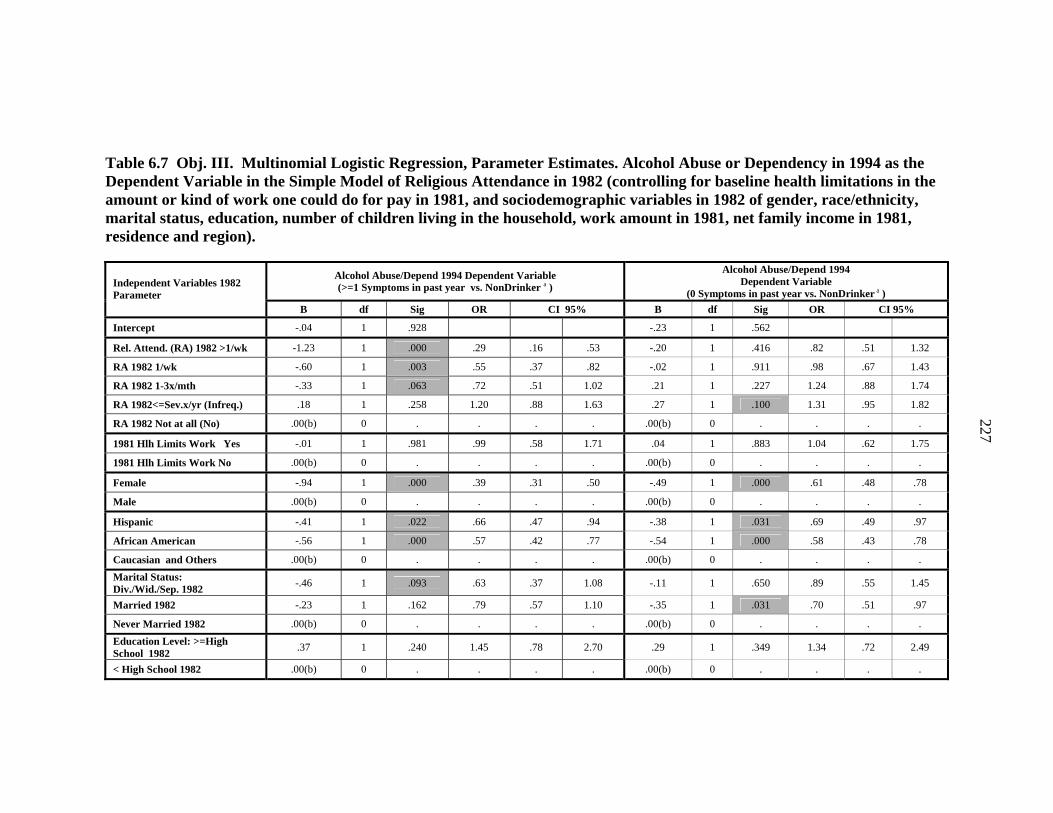
227
Table 6.7 Obj. III. Multinomial Logistic Regression, Parameter Estimates. Alcohol Abuse or Dependency in 1994 as the Dependent Variable in the Simple Model of Religious Attendance in 1982 (controlling for baseline health limitations in the amount or kind of work one could do for pay in 1981, and sociodemographic variables in 1982 of gender, race/ethnicity, marital status, education, number of children living in the household, work amount in 1981, net family income in 1981, residence and region).
Alcohol Abuse/Depend 1994 Dependent Variable (>=1 Symptoms in past year vs. NonDrinker a )
Alcohol Abuse/Depend 1994 Dependent Variable
(0 Symptoms in past year vs. NonDrinker a ) Independent Variables 1982 Parameter
B df Sig OR CI 95% B df Sig OR CI 95%
Intercept -.04 1 .928 -.23 1 .562
Rel. Attend. (RA) 1982 >1/wk -1.23 1 .000 .29 .16 .53 -.20 1 .416 .82 .51 1.32
RA 1982 1/wk -.60 1 .003 .55 .37 .82 -.02 1 .911 .98 .67 1.43
RA 1982 1-3x/mth -.33 1 .063 .72 .51 1.02 .21 1 .227 1.24 .88 1.74
RA 1982<=Sev.x/yr (Infreq.) .18 1 .258 1.20 .88 1.63 .27 1 .100 1.31 .95 1.82
RA 1982 Not at all (No) .00(b) 0 . . . . .00(b) 0 . . . .
1981 Hlh Limits Work Yes -.01 1 .981 .99 .58 1.71 .04 1 .883 1.04 .62 1.75
1981 Hlh Limits Work No .00(b) 0 . . . . .00(b) 0 . . . .
Female -.94 1 .000 .39 .31 .50 -.49 1 .000 .61 .48 .78
Male .00(b) 0 . . . . .00(b) 0 . . . .
Hispanic -.41 1 .022 .66 .47 .94 -.38 1 .031 .69 .49 .97
African American -.56 1 .000 .57 .42 .77 -.54 1 .000 .58 .43 .78
Caucasian and Others .00(b) 0 . . . . .00(b) 0 . . . .
Marital Status: Div./Wid./Sep. 1982 -.46 1 .093 .63 .37 1.08 -.11 1 .650 .89 .55 1.45
Married 1982 -.23 1 .162 .79 .57 1.10 -.35 1 .031 .70 .51 .97
Never Married 1982 .00(b) 0 . . . . .00(b) 0 . . . .
Education Level: >=High School 1982 .37 1 .240 1.45 .78 2.70 .29 1 .349 1.34 .72 2.49
< High School 1982 .00(b) 0 . . . . .00(b) 0 . . . .

228
Table 6.7 (Continued).
Alcohol Abuse/Depend 1994 Dependent Variable (>=1 Symptoms in past year vs. NonDrinker a )
Alcohol Abuse/Depend 1994 Dependent Variable
(0 Symptoms in past year vs. NonDrinker a ) Independent Variables 1982 Parameter
B df Sig OR CI 95% B df Sig OR CI 95% >=2 Children in Household 1982 -.04 1 .860 .96 .62 1.49 -.30 1 .168 .74 .48 1.14
1 Child 82 in Household 1982 .03 1 .856 1.03 .72 1.49 -.11 1 .542 .90 .63 1.28 No Children in Household 1982 .00(b) 0 . . . . .00(b) 0 . . . .
Work Full-Time 1981 .40 1 .008 1.50 1.11 2.02 .42 1 .005 1.52 1.14 2.03
Work Part-Time 1981 .00(b) 0 . . . . .00(b) 0 . . . . Net Family Income 1981 Missing .25 1 .207 1.28 .87 1.89 -.04 1 .843 .96 .66 1.40
Net Family Income 1981 Top 25% .30 1 .129 1.35 .92 1.99 .04 1 .821 1.04 .72 1.52
Net Family Income 1981 Mid 50% .10 1 .543 1.11 .80 1.53 -.05 1 .731 .95 .70 1.29
Net Family Income 1981 Lowest 25% .00(b) 0 . . . . .00(b) 0 . . . .
Residence 1982: Rural -.64 1 .000 .53 .38 .73 -.55 1 .001 .58 .42 .79
Residence 1982: Urban .00(b) 0 . . . . .00(b) 0 . . . .
Region 1982: West .30 1 .135 1.35 .91 2.01 .25 1 .205 1.29 .87 1.91
South 1982 .09 1 .611 1.10 .77 1.56 .17 1 .336 1.18 .84 1.67
North Central 1982 .19 1 .299 1.21 .84 1.74 .09 1 .639 1.09 .76 1.56
Northeast 1982 .00(b) 0 . . . . .00(b) 0 . . . . a The reference category is: No alcohol in past 30 days or since last interview 1989 day (valid skip). b This parameter is set to zero because it is redundant.
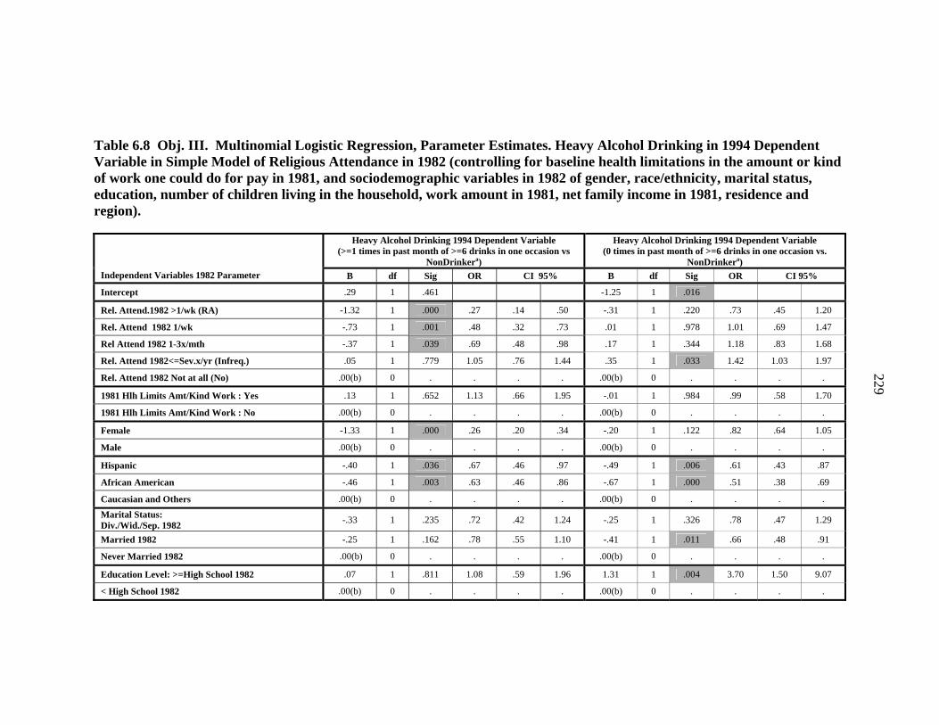
229
Table 6.8 Obj. III. Multinomial Logistic Regression, Parameter Estimates. Heavy Alcohol Drinking in 1994 Dependent Variable in Simple Model of Religious Attendance in 1982 (controlling for baseline health limitations in the amount or kind of work one could do for pay in 1981, and sociodemographic variables in 1982 of gender, race/ethnicity, marital status, education, number of children living in the household, work amount in 1981, net family income in 1981, residence and region).
Heavy Alcohol Drinking 1994 Dependent Variable (>=1 times in past month of >=6 drinks in one occasion vs
NonDrinkera)
Heavy Alcohol Drinking 1994 Dependent Variable (0 times in past month of >=6 drinks in one occasion vs.
NonDrinkera) Independent Variables 1982 Parameter B df Sig OR CI 95% B df Sig OR CI 95%
Intercept .29 1 .461 -1.25 1 .016
Rel. Attend.1982 >1/wk (RA) -1.32 1 .000 .27 .14 .50 -.31 1 .220 .73 .45 1.20
Rel. Attend 1982 1/wk -.73 1 .001 .48 .32 .73 .01 1 .978 1.01 .69 1.47
Rel Attend 1982 1-3x/mth -.37 1 .039 .69 .48 .98 .17 1 .344 1.18 .83 1.68
Rel. Attend 1982<=Sev.x/yr (Infreq.) .05 1 .779 1.05 .76 1.44 .35 1 .033 1.42 1.03 1.97
Rel. Attend 1982 Not at all (No) .00(b) 0 . . . . .00(b) 0 . . . .
1981 Hlh Limits Amt/Kind Work : Yes .13 1 .652 1.13 .66 1.95 -.01 1 .984 .99 .58 1.70
1981 Hlh Limits Amt/Kind Work : No .00(b) 0 . . . . .00(b) 0 . . . .
Female -1.33 1 .000 .26 .20 .34 -.20 1 .122 .82 .64 1.05
Male .00(b) 0 . . . . .00(b) 0 . . . .
Hispanic -.40 1 .036 .67 .46 .97 -.49 1 .006 .61 .43 .87
African American -.46 1 .003 .63 .46 .86 -.67 1 .000 .51 .38 .69
Caucasian and Others .00(b) 0 . . . . .00(b) 0 . . . .
Marital Status: Div./Wid./Sep. 1982 -.33 1 .235 .72 .42 1.24 -.25 1 .326 .78 .47 1.29
Married 1982 -.25 1 .162 .78 .55 1.10 -.41 1 .011 .66 .48 .91
Never Married 1982 .00(b) 0 . . . . .00(b) 0 . . . .
Education Level: >=High School 1982 .07 1 .811 1.08 .59 1.96 1.31 1 .004 3.70 1.50 9.07
< High School 1982 .00(b) 0 . . . . .00(b) 0 . . . .

230
Table 6.8 (Continued).
Heavy Alcohol Drinking 1994 Dependent Variable (>=1 times in past month of >=6 drinks in one occasion vs
NonDrinkera)
Heavy Alcohol Drinking 1994 Dependent Variable (0 times in past month of >=6 drinks in one occasion vs.
NonDrinkera) Independent Variables 1982 Parameter B df Sig OR CI 95% B df Sig OR CI 95%
>=2 Children in Household 1982 .23 1 .316 1.26 .80 1.98 -.41 1 .070 .66 .42 1.03
1 Child in Household 1982 .19 1 .342 1.21 .82 1.77 -.15 1 .425 .86 .61 1.24
No Children in Household 1982 .00(b) 0 . . . . .00(b) 0 . . . .
Work Full-Time 1981 .38 1 .019 1.46 1.06 2.00 .37 1 .012 1.45 1.09 1.94
Work Part-Time 1981 .00(b) 0 . . . . .00(b) 0 . . . .
Net Family Income 1981 Missing .24 1 .241 1.27 .85 1.90 -.05 1 .796 .95 .65 1.39
Net Family Income 1981 Top 25% .24 1 .244 1.27 .85 1.90 .08 1 .659 1.09 .75 1.58
Net Family Income 1981 Mid 50% .09 1 .598 1.09 .78 1.53 .00 1 .980 1.00 .73 1.36
Net Family Income 1981 Lowest 25% .00(b) 0 . . . . .00(b) 0 . . . .
Residence 1982: Rural -.52 1 .002 .59 .43 .82 -.68 1 .000 .50 .37 .69
Residence 1982: Urban .00(b) 0 . . . . .00(b) 0 . . . .
Region 1982: West .24 1 .269 1.27 .83 1.92 .27 1 .176 1.31 .89 1.94
South 1982 .12 1 .517 1.13 .78 1.63 .14 1 .438 1.15 .81 1.62
North Central 1982 .24 1 .206 1.28 .87 1.86 .00 1 .994 1.00 .70 1.44
Northeast 1982 .00(b) 0 . . . . .00(b) 0 . . . . a The reference category is: No alcohol in past 30 days or since last interview 1989 day (valid skip) . b This parameter is set to zero because it is redundant.

231
Table 6.9 Obj. III. Multinomial Logistic Regression, Parameter Estimates. Cigarette Smoking Frequency in 1994 Dependent Variable in Simple Model of Religious Attendance in 1982 (controlling for baseline health limitations in the amount or kind of work one could do for pay in 1981, and sociodemographic variables in 1982 of gender, race/ethnicity, marital status, education, number of children living in the household, work amount in 1981, net family income in 1981, residence and region).
Cigarette Smoking 1994 Dependent Variable (Smoke >= 1 pack/day vs. NonSmokera)
Cigarette Smoking 1994 Dependent Variable (Smoke < 1 pack/day vs. NonSmokera) Independent Variables 1982
Parameter B df Sig OR CI 95% B df Sig OR CI 95%
Intercept -.75 1 .092 -1.63 1 .001
Rel. Attend. 1982 >1/wk (RA) -1.44 1 .000 .24 .11 .50 -1.10 1 .006 .33 .15 .73
Rel Attend 1982 1/wk -1.12 1 .000 .33 .20 .53 -.85 1 .002 .43 .25 .73
Rel Attend 1982 1-3x/mth -1.01 1 .000 .36 .24 .55 -.53 1 .017 .59 .38 .91 Rel Attend 1982<=Sev.x/yr (Infreq.) -.51 1 .003 .60 .43 .84 .06 1 .773 1.06 .73 1.54
Rel Attend 1982 Not at all (No) .00(b) 0 . . . . .00(b) 0 . . . .
1981 Hlh Limits Work Yes .38 1 .190 1.46 .83 2.57 -.39 1 .323 .68 .31 1.46
1981 Hlh Limits Work No .00(b) 0 . . . . .00(b) 0 . . . .
Female -.49 1 .001 .61 .45 .83 .14 1 .391 1.15 .83 1.59
Male .00(b) 0 . . . . .00(b) 0 . . . .
Hispanic -1.13 1 .000 .32 .20 .52 .22 1 .340 1.25 .79 1.96
African American -.81 1 .000 .44 .30 .65 .69 1 .000 2.00 1.39 2.88
Caucasian and Others .00(b) 0 . . . . .00(b) 0 . . . .
Marital Status: Div./Wid./Sep. 1982 .72 1 .009 2.06 1.20 3.53 .08 1 .792 1.09 .58 2.02
Married 1982 .19 1 .348 1.20 .82 1.77 -.22 1 .303 .80 .52 1.22
Never Married 1982 .00(b) 0 . . . . .00(b) 0 . . . .
Education Level: >=High School 1982 -.38 1 .276 .68 .34 1.36 -.21 1 .598 .81 .37 1.76
< High School 1982 .00(b) 0 . . . . .00(b) 0 . . . .

232
Table 6.9 (Continued).
Cigarette Smoking 1994 Dependent Variable (Smoke >= 1 pack/day vs. NonSmokera)
Cigarette Smoking 1994 Dependent Variable (Smoke < 1 pack/day vs. NonSmokera) Independent Variables 1982
Parameter B df Sig OR CI 95% B df Sig OR CI 95% >=2 Children in Household 1982 .76 1 .003 2.13 1.29 3.51 .11 1 .706 1.11 .64 1.93
1 Child in Household 1982 .82 1 .000 2.28 1.50 3.46 .53 1 .017 1.69 1.10 2.62 No Children in Household 1982 .00(b) 0 . . . . .00(b) 0 . . . .
Work Full-Time1981 .04 1 .838 1.04 .73 1.48 -.21 1 .238 .81 .57 1.15
Work Part-Time 1981 .00(b) 0 . . . . .00(b) 0 . . . .
Income 1981 Missing .33 1 .171 1.39 .87 2.24 .13 1 .598 1.14 .70 1.86
Income 1981 Top 25% .35 1 .142 1.41 .89 2.24 .15 1 .533 1.17 .72 1.88
Income 1981 Mid 50% .30 1 .132 1.35 .91 1.98 .09 1 .681 1.09 .72 1.66
Income 1981 Lowest 25% .00(b) 0 . . . . .00(b) 0 . . . .
Residence 1982: Rural -.40 1 .033 .67 .46 .97 -.21 1 .317 .81 .53 1.23
Residence 1982: Urban .00(b) 0 . . . . .00(b) 0 . . . .
Region 1982: West -.06 1 .792 .94 .58 1.52 .02 1 .929 1.02 .62 1.69
South 1982 .25 1 .244 1.29 .84 1.97 .12 1 .592 1.13 .73 1.73
North Central 1982 .21 1 .324 1.24 .81 1.89 -.08 1 .746 .93 .58 1.48
Northeast 1982 .00(b) 0 . . . . .00(b) 0 . . . . a The reference category is nonsmoker (valid skip) or 0 freq. b This parameter is set to zero because it is redundant.

233
Conclusion: Summary of Objective III
The behavior factors of alcohol abuse or dependency, frequency of alcohol drinking,
and cigarette smoking mediate the relationship of religious attendance in early
adulthood to depression in mid-adulthood and, to a lesser extent, the relationship of
religious attendance in young adulthood to mental health scores in mid-adulthood.
Increasing religious attendance in young adulthood is a protective factor against
alcohol abuse or dependency, and frequency of heavy drinking and smoking.
Objective III Discussion
Justification for use of Mediator vs. Modifier
There is a debate in the literature as to whether a mediator can also be a modifier
between the association of the same independent and dependent variable. According to
an article by James and Brett, this is possible, but not according to Barron and Kenney
(James & Brett, 1984; Barron & Kenney, 1984).
Theoretically, it is expected that religious attendance influences behaviors, and that
behavior influences health. Although alcohol and cigarette smoking are significant
modifiers of the effect of religious attendance on depression and mild modifiers for
mental health, this study focuses on the theoretical testing of these behaviors to act as
mediators in order to contribute to the association between religious attendance and
depression and mental health.

234
Protective Effects of Religious Attendance on Alcohol Abuse or Dependency, Heavy
Alcohol Drinking, and Cigarette Smoking
It is interesting to find that religious attendance in young adulthood (ages 22 to 25 in
1982) has no effect on whether people use alcohol twelve years later in mid-adulthood
(ages 34 to 37). However, increasing religious attendance in young adulthood is a
strong predictor of whether an individual abuses or becomes dependent on alcohol
twelve years later.
Another important finding is that only high attendance of once to more than once per
week is protective against less frequent episodes of heavy drinking twelve years later.
In addition, heavy to moderate smoking in the mid-30s is predicted by religious
attendance twelve years earlier.
One hypothesis that might explain the protective effects of increasing attendance in
young adulthood against alcohol abuse or dependency and heavy alcohol drinking and
cigarette smoking frequency twelve years later in mid-adulthood is that those with no
religious attendance in young adulthood use alcohol or smoking as a coping
mechanism later in life, while those who are more frequent attenders as young adults
find a form of coping through religious participation, which protects them against
using other, less-healthy means of coping with the stresses of mid-adulthood. There
are no data on religious attendance in 1994, the year that alcohol and smoking factors
were measured. It would be interesting to know whether the nonattenders in 1982
remained nonattenders in 1994. If this were the case, then this might support the
possible explanation that the nonattenders engaged in risky behaviors to cope in place
of participating in religious activities as a means of coping.

235
Strengths
The theoretical pathways explaining the association between religious attendance and
health have not been studied thoroughly. This research attempts to elucidate the
mediation of behavior of alcohol abuse or dependency and frequency of cigarette
smoking to explain, at least in part, why religious attendance has an influence on
health.
The data used in the study comprise a nationally representative dataset; thus the results
can be generalized to the U.S. population from which the sample was selected—those
in their late teens living in the U.S. during the late 1970s.
Limitations
Very few variables related to lifestyle and behavior could be examined in this study.
For example, there were a series of illegal substance use questions, but the frequency
of use among those reporting such use was too low, creating unequal variance within
categories. Another key theoretical pathway, social support, could not be tested in this
study, because of the lack of social support variables available in the dataset.
The mediators were available for multiple years during the eighteen-year gap
separating attendance in young adulthood in 1982 from health status in mid-adulthood.
As mentioned in Chapter 3, however, the year 1994 was selected because it fell
between the years 1982 for attendance and 2000 for health. Alcohol frequency and
behaviors are fairly consistent across adulthood, and do not fluctuate widely (E.
Wethington, personal communication, 2005).
Another limitation of the study is that the sociodemographic control variables were
limited to 1982. Sociodemographic variables of 1994 were not added to the model.

236
Future Research Recommendations:
Other variables related to alcohol use and smoking may be tested as mediators, such as
frequency of “average number of drinks on typical days one does drink within last
month” (NLS 2004). The series of questions on alcohol behaviors could be calculated
based on the DSM-IV classification for abuse or dependency, as mentioned in Chapter
3. These new variables could be tested for possible mediation as well. Explorations
into the protective effects of religious attendance on later alcohol abuse or dependency
and frequency of heavy alcohol drinking and cigarette smoking deserve further
exploration.
Policy Implications:
Again, it is premature to recommend policy implications based on this research.
Future research into mediation may, however, provide insights to those hoping to
identify key socio-cultural factors related to religious or spiritual beliefs and practices
that contribute to improved health. Once these factors are more clearly identified,
mediating factors may be considered as preventative or coping strategies for improved
health. The implications of religious participation in young adulthood as a protective
factor against later alcohol abuse or dependency, heavy alcohol drinking, and smoking
are promising. Further research may shed light on whether health prevention strategies
with a religious or spiritual component among youth and young adults may be
effective against substance abuse later in life.

237
CHAPTER 7 Qualitative Framework
The health effects of religious and spiritual beliefs and practices within international humanitarian projects: conceptualization, theory, mediating pathways, practice and
policy
Introduction
This section provides a framework for future analysis of exploratory interviews with
researchers and professionals at international humanitarian organizations on the
influence of religious and spiritual beliefs and practices on mental and physical health,
within the context of agency projects. The major themes explored are the
conceptualizations of religiousness, spirituality, and mental and physical health, and
theorized mediating pathways, field experiences, and institutional policies.
There is growing interest and understanding among researchers of the role that socio-
cultural factors, particularly religious and spiritual beliefs and practices, have on
mental and physical health, as discussed in the literature review section in Chapter 2.
An understanding of these factors may eventually lead to improved mental and
physical health within various populations. It is thought that health projects that take
into account the socio-cultural beliefs and practices of targeted populations in design,
implementation, and evaluation are more effective than projects that do not. Many
international agencies lack effective policies with adequate guidelines to enable health
projects to account for socio-cultural beliefs and practices. Adequate policies need to
be developed within international humanitarian agencies to include adequate and
context-specific socio-cultural factors in the design, implementation, and evaluation of
health projects.

238
Justification for Qualitative Research
Viewing the relationship of religiousness and spirituality to mental and physical health
from an international perspective is not common; social scientific study of this
relationship remains an underdeveloped field within the study of epidemiology of
religion (Koenig, personal communication, 2005). Very few studies have examined
this topic from a cross-cultural or cross-national perspective within the social sciences.
The WHO initiative to include a spirituality, religiousness, and personal beliefs
component in the Quality of Life International study is a rare exception (WHOQOL
SRPB Group 2005; World Health Organization, 2002a; WHOQOL Group, 1998). Yet
it is only a pilot study, the purpose of which is to develop a survey instrument for
public use, to study spiritual, religious, and personal beliefs on quality of life. The
other main international study is the cross-sectional International Survey of the
General Social Survey, which includes questions on individual opinions and beliefs
about various issues including social issues such as socioeconomic status, family, and
race relations (General Social Survey Series, 2005). Topical modules have been added
for certain years to investigate new issues and have included various topics on medical
care, religion, religion and health, gender, and cultural issues (General Social Survey
Series, 2005). The survey is administered biannually with a unique, independently
drawn sample representative of the nations in which it is administered. In 1998 the
religion module of the survey was administered in over two dozen countries world-
wide, although most of these were located in the Western hemisphere (International
Social Survey Programme, 2005).
Objectives and Methods
The objective of the qualitative study is to provide an original analysis of the ways in
which spiritual and religious beliefs and practices, as they relate to health, are
incorporated in humanitarian projects at international governmental agencies as well

239
as nongovernmental organizations, in terms of (1) conceptualizations of religiousness,
spirituality, and health; (2) hypothesized pathways; (3) field experiences; and (4)
policy support and recommendations.
Interview Content Themes
This qualitative research is important in taking an exploratory approach to
investigating the most current projects in which international humanitarian and
missionary related organizations are involved, in regards to health programs that have
a religious/spiritual component. The main themes explored are described below. A
summary and more detailed interview guide and consent form are shown in Appendix
C.
(1a) Theories of religiousness/spirituality and health, on which health projects are
based;
(1b) Experiences/outcomes of the projects, reinforming the theories;
(2) Policy implications at the national and international level for supporting or not
supporting health projects that have a religiousness/spirituality component;
(3) Future recommendations for or thoughts about international health projects with a
religious/spirituality component: What is needed for the future in terms of policies,
resources, cooperation, and research?
Because each agency has its own background philosophies, goals, and objectives, and
because projects with religiousness/spirituality components exhibit a wide range of

240
diversity across agencies, it was important to inquire about the following background
information at the beginning of each interview:
(4) Philosophy, the mission of the agency, including goals and objectives;
(5a) Types of health projects with a socio-cultural component, including the religious
or spiritual beliefs of target populations;
(5b) History, implementation and evaluation (successes and weaknesses of such
programs);
(6) Determining which types of health projects are most and least benefited by the
incorporation of a spirituality/religiousness component.
It was important to inquire about the professional background and experiences of each
interviewee:
Professional Position
Responsibilities
Experiences/Background in international humanitarian work and health programs with
a spirituality/religiousness component.
The interviews included both fixed questions, such as those listed above, and flexible
questions, depending on the types of responses that arose during interviews. In
addition, the order of the questions was both fixed and flexible. The order followed the
described outline above, but was frequently adjusted to the type and nature of
interviewee responses.

241
Each interview was approximately one hour in length (ranging from a half hour to
three hours in length) and was audio taped with the prior permission of the
interviewee. Also, handwritten notes were taken during each interview by the
interviewer.
Sample Selection
The sample to be interviewed was selected by the use of a convenient sample. The
professionals who were selected for interview requests included personnel at
governmental and nongovernmental international humanitarian organizations, some of
which are secular and some of which have a religious affiliation. Researchers at
universities were also interviewed. Additional interviewees were contacted as a result
of recommendations offered during the initial and follow-up contacts. Additional
follow-up questions or issues to be addressed were clarified through follow-up
interviews via telephone or e-mail.
Confidentiality
Confidentiality was addressed while informing each interviewee before the initial
interview, via e-mail, of the nature of the questions, the purpose of the interview, and
its confidentiality. Interviewees were given the option of keeping their identifying
information confidential.
Human Subject Approval
Approval by the Cornell University Human Subject Review Committee was obtained
for qualitative interviewing of researchers, policy makers, and other professionals
involved in health research/programs at the international humanitarian agencies and
universities. The request was submitted and approved before the research commenced.

242
Qualitative Research Description
For approximately two months, interviews were conducted with researchers, policy
makers, and other professionals at international humanitarian organizations and
universities. Other professionals at secular and faith-based nongovernmental
organizations (NGOs) were also contacted. Leaders of faith-based missions that focus
on international health projects were also interviewed.
Methods
Since an international secondary dataset with adequate religious and spiritual and
health variables was not found for analysis, it was decided to conduct exploratory
qualitative interviews primarily with researchers at international humanitarian
organizations involved in health projects in which the socio-cultural component was
thought to be important. The exploratory interviews investigate the theoretical
conceptualizations and pathways involved in explaining the relationship of socio-
cultural beliefs and practices to health. Field experiences informing the theories and
policies of the organizations that are supportive of these socio-cultural beliefs in
design, implementation, and evaluation were also included in the qualitative
interviews.
A semi-structured, open-ended interview guide was developed to provide in-depth
analysis of the knowledge acquired about participants’ experiences related to the
themes of the interviews. The summary outline of the interview guide is provided
along with the consent form (refer to Appendix C).
This qualitative inquiry provides a descriptive, exploratory, and inductive opening-up
of new ideas and information on religiousness and spirituality in relation to health in
the international humanitarian arena (Miles & Huberman, 1994). The qualitative in-

243
person interviews provide credible anecdotal evidence at the international level for a
deeper understanding of “complex real-world contexts” contributing to the theoretical
and quantitative sections of the dissertation (Miles & Huberman, 1994).
The agencies from which interviewees were selected feature humanitarian projects
that are directly or indirectly related to health. Approximately 30 in-person interviews,
of approximately one hour each, have been conducted with representatives of various
governmental and nongovernmental organizations. Other sampling methods employed
in finding and identifying potential interviewees include the opportunistic or chain
effect, based on recommendations from initial agency contacts (Miles & Huberman,
1994).
During data collection and prior to analysis, participants were contacted (in what
sociologists term “member checks” for confirmability of findings) to discuss emerging
themes with the researchers, to solicit their input for the interpretation of the data, and
if necessary to provide clarification or correction of the information provided during
the initial interviews (Miles & Huberman, 1994). These methods increase the
objectivity of the findings (lessening the effects of researcher bias), and improve the
validity of the study.
The audio taped interviews and field notes were transcribed verbatim and checked for
accuracy. Several persons were hired to assist with transcription.
Next, the analysis will be based on grounded theory, attempting to identify categories
and concepts that emerge from the text and linking these concepts with the theory
(Denzin & Lincoln, 2003). The main and recurring themes, concepts, and issues found

244
from the transcribed interviews will be categorized. The themes and concepts are to be
compared and contrasted, using the technique of the constant comparison method
(Denzin & Lincoln, 2003). From the themes and concepts that emerge from the data, a
conceptual model will be formulated for the definitions and the role of religion and
spirituality in relation to health (including hypothesized mediating pathways to explain
this relationship, and field experiences that inform the theory and policies), within the
context of international projects.
The analysis will use the qualitative software program ATLAS to assist with the
organization of the transcribed material.
Summary
This exploratory qualitative framework and future analysis will contribute by
providing a current overview of the ways in which socio-cultural beliefs and practices,
particularly spirituality and religiousness, within the context of health projects, are
conceptualized and utilized in the field and through policies of international
humanitarian organizations.

245
CHAPTER 8 Conclusion of Dissertation
Summary of Findings
from the Three Sections of Literature Review, Quantitative Analysis and the
Qualitative Framework
Literature Review and Key Pathways
The first section of this dissertation provides a background literature review,
conceptualizations of religiousness and spirituality, and hypothesized theoretical
pathways and mediating factors for explaining the relationship of spiritual and
religious beliefs and practices to health.
Four key regrouped pathways to explain how religiousness and spirituality affect
health
This section identified and recategorized four key pathways for explaining how
religious and spiritual beliefs and practices influence health outcomes, from among a
series of possible pathways proposed by Levin (1996). These four categorized
pathways are (1) the Behavior and Lifestyle Pathway; (2) the Social Support Pathway;
(3) the Psychodynamics of Ritual, Belief, and Faith Pathway; and (4) the
Multifactorial Pathway.
Salutogenic model of the positive impact of religious beliefs and practices on health
The salutogenic model of health proposed by Antonovsky provides a framework for
conceptualizing positive health outcomes as an alternative to the pathogenic model
that is prevalent in most medical models.

246
Need to consider the negative impact of religious beliefs and practices on health
Religious participation may not always have a positive impact on health. A review of
negative studies provides a more balanced perspective on the potential negative health
effects of religious beliefs and participation.
Quantitative Analysis
Objective I
The second section of the dissertation provides a quantitative analysis examining the
cross-sectional relationship in the year 2000 of religious participation to mental and
physical health and depression and the mediating pathway of behavior and lifestyle,
among those 40 to 43 years of age, utilizing data from the National Longitudinal
Survey of Youth 79 (NLSY79).
U-shaped curvilinear relationship of religious attendance to physical health
The main findings of this research for Objective I have developed from examining the
relationship between religious attendance and physical and mental health and
depression in 2000. A positive U-shaped curvilinear relationship across religious
attendance levels and physical health in the year 2000 has been found, controlling for
gender, race, marital status, education, number of children living in the household,
work amount, and income. Moderate to infrequent attendance levels (of one to three
times per month to several times a year or less) were related to better physical health
scores, while higher attendance levels of once to more than once per week or no
attendance were related to lower physical health scores.
Religious attendance for low SES associated with better physical health scores
Some attendance among those of low SES (low education, or low work amount, or
low income) was associated with better physical health compared with no attendance.

247
For those of higher SES, religious attendance made very little difference in physical
health scores.
African Americans were shown to have better mental health and less depression with
higher attendance levels
African Americans with higher attendance levels reported better mental health scores
and lower depression scores, compared with no attendance, controlling for the
sociodemographic variables listed above (gender, marital status, education, number of
children living in the household, work amount, and income). In contrast, Caucasians
and others showed the reverse trend: lower mental health and higher depression scores
with increased attendance, and better mental health and lower depression scores with
no attendance. Hispanics fluctuated in mental health and depression scores across
various levels of attendance.
Objective II
Objective II examines the relationship of early adulthood attendance in 1982 to
physical health, mental health and depression in 2000, controlling for baseline health
limitations in 1981, and sociodemographic control variables of gender, race/ethnicity,
marital status, education level, number of children living in the household, residence,
and region. The key findings are listed below.
Attendance as young adult in 1982 was predictive of better mental health and less
depression in 2000
Early attendance in young adulthood was positively associated with better mental
health and less depression in middle adulthood, controlling for baseline health
limitations in 1981, and 1982 sociodemographic factors previously mentioned. Even
after controlling for both the 1982(previously mentioned) and the 1998

248
sociodemographic variables of marital status, number of children living in the
household, net family income, work amount, and residence, there was still a
significant relationship between young adulthood attendance in 1982 and better mental
health and less depression in 2000.
Religious affiliation of some kind in young adulthood in 1982 was predictive of better
physical health and lower depression in 2000, compared with no affiliation in 1982
Religious affiliation in young adulthood was associated with mid-adulthood physical
health and depression (without the presence of attendance 1982), and controlling for
1981 baseline health limitations and the 1982 sociodemographic variables previously
mentioned. Those with no affiliation in young adulthood reported the poorest physical
health and highest depression scores in mid-adulthood.
Being of the Jewish faith in 1982 was predictive of better physical health and lower
depression in mid-adulthood in 2000
Those who were affiliated with the Jewish faith as young adults had the highest
physical health and lowest depression scores in mid-adulthood, controlling for the
1982 sociodemographic variables listed above. There were only approximately twenty
respondents with this affiliation, so the results may not be reliable.
Consistent moderate attendance of one to three times per month from 1982 to 2000
was associated with better physical health, better mental health and lower depression
in 2000. Decrease in attendance over time was also associated with better health in
2000
No change in moderate attendance of one to three times per month from 1982 to 2000
was associated with better physical health, mental health and low depression scores in
mid-adulthood. The general trend was that no change or constant attendance (ranging

249
from more than once per week to infrequent attendance) from 1982 to 2000 was
associated with better health in 2000, compared with those who changed in
attendance. Those who reported a decreased attendance also reported better health.
Objective III
Cigarette Smoking in 1994 found to be a complete mediator of relationship between
religious attendance 1982 and mental health and depression in 2000
Frequency of cigarette smoking was a complete mediator of the relationship between
religious attendance and depression and mental health. Those who attended religious
services in young adulthood in 1982 were less likely to engage in heavy or moderate
smoking in 1994. There was a linear relationship between increasing religious
attendance, and lower odds of cigarette smoking frequency. Likewise, increasing
frequency of cigarette smoking in 1994 was related to higher depression scores in
2000.
Alcohol abuse and dependency found to be a mild partial mediator of the relationship
between religious attendance and depression
Alcohol abuse and dependency showed evidence of mild partial mediation for
religious attendance and depression.
Alcohol Drinking found to be a very mild partial mediator of the relationship between
religious attendance and depression
Heavy alcohol drinking was not a significant mediator; only whether an individual
used alcohol or not was found to be a mediator.

250
There was no evidence of mediation for any of the potential mediators of alcohol
abuse and dependency, heavy alcohol drinking, or cigarette smoking frequency for the
relationship between religious attendance 1982 and physical health 2000.
Attendance as a young adult in 1982 was protective against engaging in risky
behaviors of heavy alcohol drinking, smoking, or alcohol abuse and dependence in
1994
Respondents with higher attendance levels as young adults were less likely to engage
in such risky behaviors as alcohol abuse and dependency, heavy alcohol drinking, and
smoking, controlling for 1982 sociodemographic variables of gender, race/ethnicity,
marital status, education, work amount, income, residence, region, and baseline health
status 1981. Religious attendance was a strong predictor of later alcohol abuse and
dependency, heavy alcohol drinking, and smoking. Infrequent attendance in young
adulthood was not protective against the behaviors of alcohol abuse or dependency or
heavy alcohol drinking in mid-adulthood. However, infrequent attendance in young
adulthood was protective against heavy smoking in mid-adulthood.
Attendance as a young adult in 1982 was not found to affect or influence alcohol
drinking in 1994.
Qualitative Exploration
Development of framework for qualitative analysis
To further investigate the relationship of religiousness and health at the international
humanitarian organizational level, the last section of the dissertation develops a
qualitative framework. Exploratory interviews with researchers and professionals at
international humanitarian organizations were conducted on the influence of spiritual
and religious beliefs and practices on health, within the context of agency projects.

251
Major themes explored were the following: conceptualization of spirituality,
religiousness and health; theorized mediating pathways; field experiences; and
institutional policies. The interviews will be analyzed in the future.
Many international agencies lack effective policies with adequate guidelines to enable
health projects to account for the socio-cultural beliefs and practices of the population
being served. It is believed that the development of more adequate policies within
international humanitarian agencies to include socio-cultural factors (such as religious
or traditional beliefs and practices) in the design, implementation, and evaluation of
health projects would help to make implemented health projects more effective. This
qualitative research will explore this current thinking.
Study Strengths and Other Studies’ Findings
Quantitative Analysis
National longitudinal datasets that include adequate variables for both religiousness
and health are not common, as most national datasets are cross-sectional. Despite the
inherent limitations of using this secondary dataset of the NLSY79, this study is
among the few of which the author is aware that investigates the association of
religious attendance and self-reported physical health, mental health, and depression
cross-sectionally, over time, and testing of the mediating theoretical pathways of
behavior/lifestyle by using such a dataset. Another study by Hummer, published in
1999, examined the relationship between religious attendance and reduced risk of
mortality over a nine-year follow-up period, using a nationally representative sample
of U.S. adults (Hummer, Rogers, Nam, & Ellison, 1999). The data were obtained from
the National Health Interview Survey and linked to later mortality data. The study
results showed that people who attended religious services more than once per week
had an additional seven years in life expectancy at age 20 compared with those who

252
never attended (Hummer et al., 1999). This study found a relationship between
religious participation and reduced mortality, using national U.S. data. The
distinguishing contribution of this dissertation to the literature is that it examines,
cross-sectionally and over time, the relationship of religious participation to self-
reported physical health, mental health and depression, from well-validated health
outcome measures of the SF-12 items and the CES-Depression scale, from a nationally
representative sample of adults in the United States. The study also tests the mediating
pathway of behavior of cigarette frequency, alcohol abuse or dependency and heavy
drinking, to help explain how religious participation may affect health outcomes.
Studies using national data from other countries have examined the relationship
between religious participation and various health outcomes. For example, a national
longitudinal study in the Netherlands among older Dutch citizens found that religious
attendance was associated with fewer depressive symptoms over a six-year period
(Braam et al., 2004). A cross-sectional national Canadian study on spiritual and
religious involvement and depressive symptoms found that those with higher levels of
attendance reported fewer depressive symptoms, controlling for demographic, social
and health variables (Baetz et al., 2004).
This dissertation research has explored interactions between religious attendance and
change in attendance with sociodemographic variables (including race/ethnicity,
education, number of children living in the household, work amount, and net family
income), as well as with baseline health limitations and the subsequent interaction
effects across scores for physical health, mental health and depression. The present
study provides evidence that different groups, such as those of low socio-economic
status, and African Americans, interact with religious attendance in different ways.

253
Religious attendance may serve different purposes among different groups. For
example, the justification for hypothesizing the interaction of ethnicity and education
with attendance to predict mental and physical health outcomes is found in previous
research, which has shown that ethnicity, education levels, and number of children are
independently related to physical and mental health outcomes (Rodriguez, Allen,
Frongillo, & Chandra, 1999). There is also some evidence that the determinants of
depression differ among Caucasians and African Americans (Rodriguez et al., 1999).
Other studies have investigated relationships between religiousness and health among
African Americans. A study on religion, race/ethnicity, and self-reported health among
Caucasians, African Americans and Hispanics living in low socio-economic status
neighborhoods in Texas found that African Americans reported lower mental health
scores and self-rated health (Franzini, Ribble, & Wingfield, 2005). However, being
African American was indirectly associated with better mental health through
religious participation, but indirectly associated with poorer mental and physical
health with non-organized religiousness, measured by frequency of prayer and
importance of beliefs (Franzini, Ribble, & Wingfield, 2005).
Another study, conducted among older men, found that African Americans reported
fewer depressive symptoms, which was strongly associated with religious coping
(Koenig et al., 1992; Taylor, Chatters, & Levin, 2004). An article by Levin, Chatters,
and Taylor reviews many studies on religion and health among African Americans and
concludes that most studies show a protective effect of religiousness against
depressive symptoms and psychological distress (Levin, Chatters, & Taylor, 2005).

254
The findings of this current research project—that attendance protects against risky
behaviors of alcohol and cigarette smoking behaviors—further substantiate other
findings within the literature on this topic (Whooley et al., 2002; Koenig et al., 1994).
For example, a study by Whooley et al. (2002) found that young adults who attended
religious services reported lower rates of cigarette use, with lasting effects up to three
years later. Koenig, McCuollough, and Larson reviewed a number of studies that have
shown consistently that more frequent religious attendance, as well as private religious
practices, and religious importance, were all predictors of decreased alcohol and drug
use among adults and adolescents (Koenig et al., 2001).
Qualitative Exploratory Framework
Little research has been conducted on how international humanitarian organizations
take into account the spiritual and religious beliefs and practices of targeted
populations of particular health projects. Similarly, little research has been developed
from an international perspective on the relationship between beliefs and health
outcomes. This exploratory qualitative framework serves as an initial exploration of
current thinking and practices within international humanitarian organizations
pertaining to the relationship between beliefs and health within the context of their
research, health projects, and populations being served by these health projects.
Study Limitations
Quantitative Analysis
The limitations of the data used in this quantitative analysis include having a small
number of religious and physical and mental health variables available for only a few
years during the 25-year duration of the study.

255
Another limitation of this study, and other studies on the effects of religious
participation on health, is the problem of self-selection bias (Sloan, 2005; Hummer et
al., 1999). Selection bias is a common problem for most observational studies. People
who attend religious services more often may differ demographically from those who
do not (Hummer et al., 1999). To account for these potential differences, the analysis
controlled for the sociodemographic variables of gender, race/ethnicity, education,
marital status, number of children living in the household, work amount, net family
income, region, and type of residence (urban or rural).
Another possible source of self-selection bias is the difference in health status between
attenders and non-attenders. For the cross-sectional data in objective I, it is unclear
whether those who do not attend religious services are composed of a large number of
individuals who are too ill to be able to attend. Likewise, for those who attend
frequently, it is unclear whether these individuals are ill and thus attending religious
services to be able to cope. This may explain the U-shaped trend in religious
attendance in the data for the physical health outcome. Those at the two extremes of
attendance, high attendance of more than once per week and no attendance, report the
lowest physical health scores, while those of moderate attendance report the best
physical health scores. This self-selection bias is reduced to some degree in that the
data uses non-institutionalized individuals (Hummer et al., 1999). Thus it excludes
some of the least healthy or mobility-limited adults from the study.
Religious attendance may simply be an indicator of a healthier status rather than a
cause of better health (Bagiella, Hong, & Sloan, 2005). Those individuals who choose
to attend religious services may simply be healthier than those who do not attend
(Bagiella et al., 2005). They may exhibit or possess other characteristics that promote

256
their health. Attendance at religious services may be a result of their better health from
other causes, not necessarily from religious participation. For example, they may be
more socially involved in the community, not just in religious services, or they may
lead healthier lifestyles, of which religious participation is a result and not necessarily
a cause.
The Objective II longitudinal model attempted to reduce selection bias. The model
examined the relationship between change in religious attendance over time from 1982
to 2000 to later physical health, mental health, and depression scores in 2000, and
attempted to control selection bias by controlling for baseline “health limitations in the
amount or kind of work a respondent could do for pay in 1981.”
Those individuals who reported an increase in attendance also reported lower scores
for physical health, mental health, and higher depression, compared with those who
reported no change in attendance over time. Those individuals who reported an
increase in attendance over time may have experienced an illness which prompted
them to increase participation as a coping strategy. Controlling for baseline health
limitations in 1981, the year before the 1982 religious participation was measured,
helps to lessen the possible effects of selection bias.
Another limitation of this research and other studies on religious participation and
health is the problem of residual confounding (Sloan, 2005). The models in this study
do not control for participation in other community activities. Religious participation
itself may not be the only factor associated with the observed mental and physical
health outcomes. Rather it may be a part of a broader concept of “engagement in the

257
community and social activities” that is associated with better mental and physical
health outcomes (Sloan, 2005, p. 2).
Qualitative Analysis
The qualitative exploratory research provides a framework for future analysis of the
conducted interviews. This sample may not be representative of international
humanitarian organizations because of the use of a convenient sample formed through
previous contacts and the chain effect of sample selection.
Future Recommendations
Other suggestions to build on the findings of the present research include studying the
effects of religious attendance among different groups separately. A combination of
quantitative and qualitative research pertaining to different groups may provide
insights into the nature of interactions with SES, race/ethnicity, and marital status. It
would be interesting to examine different age groups to see if similar effects are found,
using different cohorts of the National Longitudinal Survey, such as the children of the
mothers of the NLSY79.
Future research possibilities include expanding upon the qualitative interviews to be
more inclusive of other international agencies, not just a select few, to learn how
religious and spiritual belief and practices in relation to health are understood by
international humanitarian organizations, in conceptualizations, field experiences and
policies. It would also be interesting to conduct focus groups and individual interviews
with people from various faith and cultural backgrounds to obtain a deeper
understanding at the individual and group level of personal, cultural, and religious
beliefs and practices to understand better how each perceives its impact on individual
mental and physical health.

258
Possible Policy Implications of the Research
Overall possible tentative policy implications based on the findings of this study are
suggested. It should be stressed that these are only potential policy implications, based
on these study findings alone.
Preventative and therapeutic physical and mental health community programs may
find it effective to collaborate with religious organizations to promote better health,
particularly for the marginalized of society, among the poor (those of low socio-
economic status), minorities (particularly African Americans), and among young
adults. The quantitative research findings suggest that religious participation has
physical and mental health benefits, particularly for these groups of society. Those of
low socio-economic status who attended religious services reported better physical
health scores than those of low socioeconomic status who did not attend. Participation
among African Americans was associated with lower depression scores compared
with the experiences of other ethnicities and races. Religious participation in young
adulthood showed evidence of a protective effect against engaging in risky behaviors
of alcohol abuse or dependency, and heavy drinking twelve years later. In addition, the
results show that even infrequent attendance confers health benefits compared with
non-attendance.
Participation may reduce the stressors that these often marginalized groups of
society—the poor, African Americans, and young adults—uniquely face. Participation
may promote opportunities for social support and coping strategies. Further studies
investigating the relationship between religious participation and mental and physical
health outcomes are recommended to substantiate the findings before any policies are

259
implemented. Before these policy recommendations are implemented in a large-scale
national setting, they should be tested in smaller, localized pilot programs.
There are potential long-term applications of this quantitative research and future
qualitative research. From an improved understanding of the relationship between
religiousness and mental and physical health, national or international humanitarian
health projects with a religious or spiritual component could possibly be developed for
a more integrative and long-lasting impact on the health of the populations being
served. Spiritual and religious beliefs and practices are often integral to the lives of
those who are marginalized within society. Health projects which take into account the
religious and spiritual beliefs and practices of the targeted population may be more
effective in their mission of health care and prevention.

260
APPENDIX A Quantitative Results
Objective One

261
Table A.1 Obj. I. ANOVA (Tests of Between Subject Effects) Simple, One Two-way Interactions and Full Model (Three-Two-way and Two Three-way Interactions) of Religious Attendance in 2000 interacting with Education in 2000, Work Amount in 1999 and Income in 1999 on Physical Health Composite Score in 2000 (SF-12 PCS; controlling for sociodemographic variables in 2000 of gender, race/ethnicity, marital status, education, number of children living in the household, work amount in 1999 and net family income in 1999).
Models Simple
1 2-way Educ.*
Rel. Attend
1 2-way
Work*Rel.
Attend
1 2-way
Incom. *Rel.
Attend
Full
Model 3 2-way Int.
Full
Model 2 3-way Int.
Source Independent Var. df F Sig df F Sig df F Sig d
f F Sig df F Sig d
f F Sig
Corrected Model 18 21.8 .00 26 15.8 .00 22 18.7 .00 14.1 .00 4
2 10.9 .00 83 6.5 .00
Intercept 1 13914.4 .00 13547.3 .00 13932.
4 .00 13894.0 .00 13574.6 .00 10811.0 .00
Religious Attendance 2000 4 2.0 .09 4.8 .00 5.6 .00 2.3 .05 6.4 .00 6.7 .00
Gender 1 2.2 .14 1.9 .16 2.6 .10 1.9 .17 1.9 .17 3.2 .07
Race/ethnicity 2 2.1 .13 1.9 .14 2.2 .11 2.0 .13 1.9 .15 1.4 .26
Marital Status 2000 3 1.0 .38 1.1 .36 .8 .51 1.1 .34 1.0 .38 1.4 .24
Education 2000 2 4.0 .02 4.5 .01 3.8 .02 3.7 .02 3.4 .03 2.6 .08
Child # living in househld. 2000 2 4.9 .01 5.1 .01 5.0 .01 4.9 .01 5.1 .01 4.0 .02
Work Amount 1999 1 170.3 .00 169.5 .00 179.4 .00 166.5 .00 166.2 .00 127.0 .00
Net Family Income 1999 3 11.3 .00 11.4 .00 11.5 .00 14.9 .00 14.4 .00 8.0 .00
Rel. Attend * Education 8 2.2 .02 1.9 .06 2.5 .01
College/Grad (>HS) 0.9 .89 3.0 .02
High School (HS) 1.0 .43 2.7 .03
None/Grammar (<HS) 4.6 .00 4.7 .00 4
Rel. Attend * Work Amount 4 4.4 .00 3.4 .01 2.9 .02
0 – 20 hrs/wk (PT) .3 .89 2.3 .06
>20 ->40 hrs/wk (FT) 6.2 .00 7.2 .00 1

262
Table A.1 (Continued).
Models Simple
1 2-way Educ.*
Rel. Attend
1 2-way
Work*Rel.
Attend
1 2-way Incom. *Rel. Attend
Full Model
3 2-way Int.
Full Model
2 3-way Int.
Source Independ. Var. 2000 df F Sig df F Sig df F Sig. df F Sig. df F Sig. df F Sig
. Rel. Attend * Income 12 2.3 .01 2.1 .01 0.5 .91
Missing 3.9 .00 5.1 .00
Top 25% (>=$70,000) .2 .93 2.7 .03 Mid 50% ($ >=20,600 >= 69800) .7 .60 5.1 .00
Lowest 25% (<=$20,516) 3.9 .00 5.3 .00
Rel. Attend*Work*Income 15 2.5 .00
FT * Missing .92 .45
FT * Top 25% 1.7 .16
FT* Mid 50% 1.5 .21
FT* Lowest 25% .8 .53
PT* Missing 1.9 .11
PT*Top 25% 1.4 .24
PT*Mid 50% 3.3 .01
PT*Lowest 25% 3.0 .02
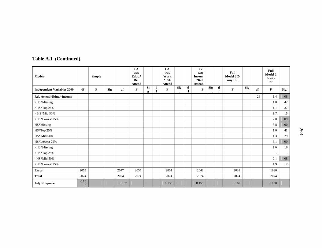
263
Table A.1 (Continued).
Models Simple
1 2-way
Educ.* Rel.
Attend
1 2-way
Work*Rel.
Attend
1 2-way
Incom. *Rel.
Attend
Full
Model 3 2-way Int.
Full Model 2 3-way
Int.
Independent Variables 2000 df F Sig df F Sig
df F Sig
. df F Sig
. df F Sig
. df F Sig.
Rel. Attend*Educ.*Income 26 1.4 .08
>HS*Missing 1.0 .42
>HS*Top 25% 1.1 .37
> HS*Mid 50% 1.7 .15
>HS*Lowest 25% 2.0 .09
HS*Missing 5.8 .00
HS*Top 25% 1.0 .41
HS* Mid 50% 1.3 .29
HS*Lowest 25% 5.1 .00
<HS*Missing 1.6 .18
<HS*Top 25% . .
<HS*Mid 50% 2.1 .08
<HS*Lowest 25% 1.9 .12
Error 2055 2047 2055 2051 2043 2031 1990
Total 2074 2074 2074 2074 2074 2074 2074
Adj. R Squared 0.153 0.157 0.158 0.159 0.167 0.180

264
Table A.2. Obj. I. Simple, (One Two-way Interactions and Full Model (Three Two-way) Interactions of Religious Attendance in 2000 interacting with Education, Work and Income on Physical Health Composite Score (SF-12 PCS) in 2000 (controlling for socio-demographic variables in 2000 of gender, race/ethnicity, marital status, education, number of children living in the household, work and income).
Dependent Variable: PCS2000 SF-12 PCS 2000 Models Simple 1 2way Interaction of
Education *Religious Attendance
1 2-way Interaction of Work Amount*Religious
Attendance
1 2-way Interaction of Net Family Income*Religious
Attendance
3 2-way Interact. Educ. * Rel. Attend, Work * Rel. Attend, Inc. * Rel. Attend
Independent Variables 2000
B Sig. CI B Sig CI B Sig CI B Sig. CI B Sig. CI
Intercept 43.4 .00 40.9 45.8 36.0 .00 30.5 41.5 40.0 .00 36.9 43.1
40.2
.00 37.0 43.3
32.4 .00 26.6 38.2
Rel. Attend >1/wk .2 .73 -1.1 1.5 8.9 .01 2.2 15.6 2.8 .05 -.01 5.6 4.9 .00 2.2 7.6 12.5 .00 5.5 19.5
Rel. Attend 1/wk 1.1 .09 -0.2 2.3 5.3 .11 -1.2 11.8 5.0 .00 2.2 7.8 4.9 .00 2.2 7.5 9.9 .01 3.0 16.7
Rel. Attend 1-3/mth 1.1 .07 -0.1 2.4 12.7 .00 6.1 19.3 5.3 .00 2.4 8.2 3.5 .01 .7 6.2 15.9 .00 8.9 22.9
Rel. Attend <=Sev.x/yr (Infreq.)
1.4 .04 0.1 2.6 10.7 .00 4.0 17.3 6.4 .00 3.5 9.2 4.1 .01 1.1 7.1 15.0 .00 7.9 22.2
Rel. Attend Not at all (No)
0(a) . . . 0(a) . . . 0(a) . . . 0(a) . . . 0(a) . . .
Female -.5 .14 -1.2 .0.2 -.5 .16 -1.2 .2 -.6 .10 -1.3 .1 -.5 .17 -1.2 .2 -.5 .17 -1.2 .2
Male 0(a) . . . 0(a) . . . 0(a) . . . 0(a) . . . 0(a) . . .
Hispanic -.9 .05 -1.9 -.02 -.9 .06 -1.8 .0 -1.0 .04 -1.9 -.05 -.9 .05 -1.8 .0 -.9 .06 -1.8 .0
African American -.4 .30 -1.3 .4 -.5 .28 -1.3 .4 -.4 .29 -1.3 .4 -.5 .27 -1.3 .4 -.5 .27 -1.3 .4
Caucasian & others 0(a) . . . 0(a) . . . 0(a) . . . 0(a) . . . 0(a) . . .
Widowed/Separated -1.0 .20 -2.5 .5 -1.0 .20 -2.5 .5 -.9 .26 -2.4 .6 -1.0 .20 -2.5 .5 -1.0 .19 -2.5 .5
Divorced -.7 .24 -1.9 .5 -.7 .23 -1.9 .5 -.6 .30 -1.8 .5 -.9 .14 -2.0 .3 -.8 .17 -2.0 .4
Married -.1 .86 -1.2 1.0 -.1 .91 -1.1 1.0 -.1 .85 -1.2 1.0 -.2 .66 -1.3 .8 -.3 .64 -1.3 .8
Never Married 0(a) . . . 0(a) . . . 0(a) . . . 0(a) . . . 0(a) . . .
> High School (HS) 1.5 .13 -.5 3.5 9.3 .00 3.7 14.8 1.4 .16 -.6 3.3 1.6 .11 -.4 3.5 7.7 .01 2.1 13.3
High School .5 .60 -1.4 2.4 7.9 .01 2.4 13.5 .4 .66 -1.5 2.3 .7 .50 -1.3 2.6 7.3 .01 1.6 12.8
< High School 0(a) . . . 0(a) . . . 0(a) . . . 0(a) . . . 0(a) . . .

265
Table A.2 (Continued).
Models Simple Interaction of Education *Religious Attendance
Interaction of Work Amount*Religious
Attendance
Interaction of Net Family Income*Religious
Attendance
3 2-way Interaction of Educ. * Rel. Attend, Work Amt. * Rel. Attend, Income * Rel.
Attend Independent Variables 2000
B Sig.
CI B Sig CI B Sig CI B Sig. CI B Sig. CI
>=2 Children 1.0 .03 .1 1.9 1.0 .03 .1 1.9 1.0 .02 .1 1.9 1.0 .03 .1 1.9 1.1 .02 .2 1.9
1 Child -.4 .47 -1.4 .7 -.4 .47 -1.4 .6 -.3 .51 -1.4 .7 -.4 .50 -1.4 .7 -.3 .57 -1.3 .7
No Children 0(a) . . . 0(a) . . . 0(a) . . . 0(a) . . . 0(a) . . .
Work>20 hrs/wk (FT)
6.1 .00 5.2 7.0 6.1 .00 5.1 7.0 10.4 .00 7.8 12.9
6.0 .00 5.1 6.9 9.0 .00 6.3 11.7
0-20 hrs/wk (PT) 0(a) . . . 0(a) . . . 0(a) . . . 0(a) . . . 0(a) . . .
Income Missing 2.1 .00 .9 3.2 2.1 .00 1.0 3.2 2.0 .00 .9 3.2 7.0 .00 3.7 10.3
6.5 .00 2.8 9.6
Income Top 25% 3.3 .00 2.0 4.5 3.3 .00 2.0 4.5 3.3 .00 2.0 4.5 7.4 .00 4.0 10.7
6.3 .00 3.0 10.0
Income Mid 50% 2.8 .00 1.8 3.8 2.8 .00 1.8 3.8 2.8 .00 1.8 3.8 6.5 .00 3.7 9.2 5.4 .00 2.5 8.3
Income Lowest 25% 0(a) . . . 0(a) . . . 0(a) . . . 0(a) . . . 0(a) . . .
Rel. Attend >1/wk * >HS
-9.2 .01 -16.2 -2.3 -7.1 .05 -14.1 .01
Rel Attend 1 wk * HS -8.7 .01 -15.7 -1.8 -7.5 .04 -14.4 -.49
Rel Att. 1/wk * < HS 0(a) . . . 0(a) . . .
Rel Att. 1/wk * >HS -4.3 .20 -11.0 2.4 -2.5 .47 -9.3 4.3
Rel Att. 1/wk * HS -4.4 .20 -11.1 2.3 -3.6 .30 -10.3 3.2
RelAtt. 1/wk * < HS 0(a) . . . 0(a) . . .
RelAtt. 1-3/mth * >HS
-12.4 .00 -19.2 -5.6 -10.8 .00 -17.7 -3.8
RelAtt. 1-3/mth * HS -11.5 .00 -18.4 -4.7 -10.7 .00 -17.6 -3.8
RelAtt.1-3/mth *<HS 0(a) . . . 0(a) . . .

266
Table A.2 (Continued).
Models Simple Interaction of Education *Religious Attendance
Interaction of Work Amount*Religious
Attendance
Interaction of Net Family Income*Religious
Attendance
3 2-way Interaction of Educ. * Rel. Attend,
Work Amt. * Rel. Attend, Income * Rel. Attend
Independent Variables 2000
B Sig.
CI B Sig CI B Sig CI B Sig. CI B Sig. CI
RA Infreq. * >HS -9.9 .00 -16.8 -3.0 -8.3 .02 -15.3
-1.3
Rel. Attend Infreq. * HS
-9.4 .01 -16.4 -2.5
-8.7 .02 -15.
7
-1.7
Rel. Attend Infreq. * <HS
0(a) . . . 0(a) . . .
Rel. Attend No * >HS 0(a) . . . 0(a) . . .
Rel. Attend No * HS 0(a) . . . 0(a) . . .
Rel. Attend No * <HS 0(a) . . . 0(a) . . .
Rel. Attend >1/wk *FT
-3.2 .05 -6.3 -.1 -1.3 .44 -4.6
2.0
Rel. Attend >1/wk *PT
0(a) . . . 0(a) . . .
Rel. Attend 1/wk *FT -4.9 .00 -8.0 -1.8 -3.5 .04 -6.7
-.2
Rel. Attend 1/wk * PT
0(a) . . . 0(a) . . .
Rel. Attend 1-3/mth* FT
-5.2 .00 -8.4 -2.0 -4.1 .02 -7.4
-.7
Rel. Attend 1-3/mth* PT
0(a) . . . 0(a) . . .
Rel. Attend Infreq* FT
-6.2 .00 -9.4 -3.0 -5.2 .00 -8.5
-1.8
Rel. Attend. Infreq*PT
0(a) . . . 0(a) . . .
Rel. Attend No*FT 0(a) . . . 0(a) . . .
Rel. Attend No*PT 0(a) . . . 0(a) . . .

267
Table A.2 (Continued).
Models Simple Interaction of Education *Religious Attendance
Interaction of Work Amount*Religious
Attendance
Interaction of Net Family Income*Religious Attendance
3 2-way Interaction of Educ. * Rel. Attend, Work Amt. * Rel.
Attend, Income * Rel. Attend
Independent Variables 2000 B Sig. CI B Sig CI B Sig CI B Sig. CI B Sig. CI Rel. Attend (RA) >1/wk *Missing Income
-8.8 .00 -12.8 -4.9 -8.2 .00 -12.3
-4.1
RA>1/wk *Top25% Income -5.5 .01 -9.6 -1.5 -5.1 .02 -9.3 -.8
RA*Mid50% Income -5.0 .00 -8.3 -1.8 -4.6 .01 -8.0 -1.0
RA>1/wk *Low25% Income 0(a) . . . 0(a) . . .
RA1/wk *Missing Income -5.5 .01 -9.3 -1.6 -4.6 .02 -8.6 -.7
RA1/wk *Top25% Income -4.6 .02 -8.5 -.8 -4.0 .05 -8.0 .0
RA1/wk *Mid50% Income -4.6 .01 -7.8 -1.4 -3.5 .04 -6.9 -.1
RA1/wk *Low25% Income 0(a) . . . 0(a) . . .
RA 1-3/mth*Missing Income -2.9 .14 -6.9 1.0 -1.8 .40 -5.9 2.3
RA1-3/mth *Top25% Income -3.5 .08 -7.5 .4 -1.8 .38 -6.0 2.3
RA1-3/mth*Mid50% Income -2.6 .12 -5.9 .7 -1.1 .55 -4.5 2.4
RA1-3/mth*Low25% Income 0(a) . . . 0(a) . . .
RA Infreq*Missing Income -4.3 .04 -8.5 -.2 -3.0 .17 -7.3 1.3
RA Infreq. *Top25% Income -3.7 .08 -7.8 .5 -2.0 .37 -6.3 2.3
RA Infreq *Mid50% Income -3.1 .09 -6.7 .5 -1.3 .50 -5.0 2.4
RA Infreq* Low 25% Income 0(a) . . . 0(a) . . .
RA No *Missing Income 0(a) . . . 0(a) . . .
RA No* Top25% Income 0(a) . . . 0(a) . . .
RA No*Mid50% Income 0(a) . . . 0(a) . . .
RA No*Low25% Income 0(a) . . . 0(a) . . .
Adj. R Squared 0.153 0.158 .159 0.167 .180 a Note: This parameter is set to zero because it is redundant.

268
Not at all<=Sev./yr1-3/mth1/wk>1/wk
Religious Attendance 2000
54.00
52.00
50.00
48.00
46.00
44.00
42.00
40.00
Estim
ated
Mar
gina
l Mea
ns
None/GrammarHigh SchoolCollege/Grad School
Education 2000 3levels
Estimated Marginal Means of Physical Health Composite Score (SF-12, PCS)2000
Figure A.1 Obj. I. Model of Physical Composite Score (PCS) in 2000 with the One Two-way Interaction of Religious Attendance in 2000 with Education in 2000 (controlling for socio-demographic variables in 2000 of gender, race/ethnicity, marital status, education, number of children living in household, work amount in 1999 and net family income in 1999).

269
Not at all<=Sev./yr1-3/mth1/wk>1/wk
Religious Attendance 2000
52.50
50.00
47.50
45.00
42.50
40.00
Estim
ated
Mar
gina
l Mea
ns
0 to 20 hrs/wk> 20 hrs/wk
Work Amt 2000 <pt vs> pt
Estimated Marginal Means of Physical Health Composite Score (SF-12, PCS)2000
Figure A.2 Obj. I. Model of Physical Health Composite Score (SF-12 PCS) in 2000 with the One Two-way Interaction of Religious Attendance in 2000 with Work Amount in 1999 (controlling for socio-demographic variables in 2000 of gender, race/ethnicity, marital status, education, number of children living in household, work amount 1999 and net family income 1999).

270
Not at all<=Sev./yr1-3/mth1/wk>1/wk
Religious Attendance 2000
50.00
48.00
46.00
44.00
42.00
Estim
ated
Mar
gina
l Mea
ns
lowest 25%(<=$20,516)
mid 50% ($ >=20,600>= 69800)
Top 25% (>=$70,000)Missing
Income 2000 25 %50% 75%
Estimated Marginal Means of Physical Health Composite Score (SF-12, PCS)2000
.
Figure A.3 Obj. I. Model of Physical Composite Score (SF-12 PCS) in 2000 with the One Two-way Interaction of Religious Attendance in 2000 with Net Family Income in 1999 (controlling for key socio-demographic variables in 2000 of gender, race/ethnicity, marital status, education, number of children living in household, work amount in 1999 and net family income in 1999).

271
Not at all<=Sev./yr1-3/mth1/wk>1/wk
Religious Attendance 2000
54.00
52.00
50.00
48.00
46.00
44.00
42.00
40.00
Estim
ated
Mar
gina
l Mea
ns
None/GrammarHigh SchoolCollege/Grad School
Education 2000 3levels
Estimated Marginal Means of Physical Health Composite Score (SF-12, PCS)2000
Figure A.4 Obj. I. Model of Physical Health Composite Score (SF-12 PCS) in 2000 with the One Two-way Interaction of Religious Attendance in 2000 with Education in 2000 (in the presence of the Two-way interactions of religious attendance in 2000 with work amount in 1999 and religious attendance in 2000 with net family income in 1999; controlling for socio-demographic variables in 2000 of gender, race/ethnicity, marital status, education, number of children living in household, work amount 1999 and net family income 1999).

272
Not at all<=Sev./yr1-3/mth1/wk>1/wk
Religious Attendance 2000
54.00
52.00
50.00
48.00
46.00
44.00
42.00
40.00
Estim
ated
Mar
gina
l Mea
ns
0 to 20 hrs/wk> 20 hrs/wk
Work Amt 2000 <pt vs> pt
Estimated Marginal Means of Physical Health Composite Score (SF-12, PCS)2000
Figure A.5 Obj I. Model of Physical Health Composite Score (SF-12 PCS) in 2000 with the One Two-way of Interaction of Religious Attendance in 2000 with Work Amount in 1999 (in the presence of the Two-way interactions of religious attendance in 2000 with education in 2000 and religious attendance in 2000 with net family income in 1999; controlling for socio-demographic variables in 2000 of gender, race/ethnicity, marital status, education, number of children living in household, work amount in 1999 and net family income in 1999).

273
Not at all<=Sev./yr1-3/mth1/wk>1/wk
Religious Attendance 2000
52.50
50.00
47.50
45.00
42.50
40.00
Estim
ated
Mar
gina
l Mea
ns
lowest 25%(<=$20,516)
mid 50% ($ >=20,600>= 69800)
Top 25% (>=$70,000)Missing
Income 2000:low 25%;mid-50%; top 25%
Estimated Marginal Means of Physical Health Composite Score (SF-12, PCS)2000
Figure A.6 Obj I. Model of Physical Health Composite Score (SF-12 PCS) in 2000 with the One Two-way Interaction of Religious Attendance in 2000 with Net Family Income in 1999 (in the presence of the Two-way interactions of religious attendance in 2000 with education in 2000 and religious attendance in 2000 with work amount in 1999; controlling for socio-demographic variables in 2000 of gender, race/ethnicity, marital status, education, number of children living in household, work amount in 1999 and net family income in 1999).
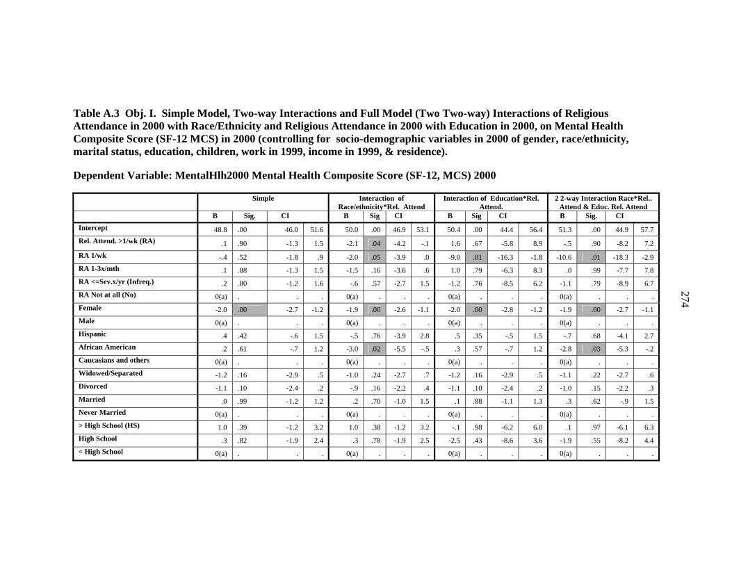
274
Table A.3 Obj. I. Simple Model, Two-way Interactions and Full Model (Two Two-way) Interactions of Religious Attendance in 2000 with Race/Ethnicity and Religious Attendance in 2000 with Education in 2000, on Mental Health Composite Score (SF-12 MCS) in 2000 (controlling for socio-demographic variables in 2000 of gender, race/ethnicity, marital status, education, children, work in 1999, income in 1999, & residence).
Dependent Variable: MentalHlh2000 Mental Health Composite Score (SF-12, MCS) 2000
Simple Interaction of Race/ethnicity*Rel. Attend
Interaction of Education*Rel. Attend.
2 2-way Interaction Race*Rel.. Attend & Educ. Rel. Attend
B Sig. CI B Sig CI B Sig CI B Sig. CI Intercept 48.8 .00 46.0 51.6 50.0 .00 46.9 53.1 50.4 .00 44.4 56.4 51.3 .00 44.9 57.7 Rel. Attend. >1/wk (RA) .1 .90 -1.3 1.5 -2.1 .04 -4.2 -.1 1.6 .67 -5.8 8.9 -.5 .90 -8.2 7.2 RA 1/wk -.4 .52 -1.8 .9 -2.0 .05 -3.9 .0 -9.0 .01 -16.3 -1.8 -10.6 .01 -18.3 -2.9 RA 1-3x/mth .1 .88 -1.3 1.5 -1.5 .16 -3.6 .6 1.0 .79 -6.3 8.3 .0 .99 -7.7 7.8 RA <=Sev.x/yr (Infreq.) .2 .80 -1.2 1.6 -.6 .57 -2.7 1.5 -1.2 .76 -8.5 6.2 -1.1 .79 -8.9 6.7 RA Not at all (No) 0(a) . . . 0(a) . . . 0(a) . . . 0(a) . . . Female -2.0 .00 -2.7 -1.2 -1.9 .00 -2.6 -1.1 -2.0 .00 -2.8 -1.2 -1.9 .00 -2.7 -1.1 Male 0(a) . . . 0(a) . . . 0(a) . . . 0(a) . . . Hispanic .4 .42 -.6 1.5 -.5 .76 -3.9 2.8 .5 .35 -.5 1.5 -.7 .68 -4.1 2.7 African American .2 .61 -.7 1.2 -3.0 .02 -5.5 -.5 .3 .57 -.7 1.2 -2.8 .03 -5.3 -.2 Caucasians and others 0(a) . . . 0(a) . . . 0(a) . . . 0(a) . . . Widowed/Separated -1.2 .16 -2.9 .5 -1.0 .24 -2.7 .7 -1.2 .16 -2.9 .5 -1.1 .22 -2.7 .6 Divorced -1.1 .10 -2.4 .2 -.9 .16 -2.2 .4 -1.1 .10 -2.4 .2 -1.0 .15 -2.2 .3 Married .0 .99 -1.2 1.2 .2 .70 -1.0 1.5 .1 .88 -1.1 1.3 .3 .62 -.9 1.5 Never Married 0(a) . . . 0(a) . . . 0(a) . . . 0(a) . . . > High School (HS) 1.0 .39 -1.2 3.2 1.0 .38 -1.2 3.2 -.1 .98 -6.2 6.0 .1 .97 -6.1 6.3 High School .3 .82 -1.9 2.4 .3 .78 -1.9 2.5 -2.5 .43 -8.6 3.6 -1.9 .55 -8.2 4.4 < High School 0(a) . . . 0(a) . . . 0(a) . . . 0(a) . . .

275
Table A.3 (Continued).
Simple Interaction of Race and Religious Attendance
Interaction of Education*Religious
Attendance
2 2-way Interaction of Race*Religious. Attendance
and Education*Religious Attendance
B Sig. CI B Sig CI B Sig CI B Sig. CI >=2 Children Living in Household .4 .45 -.6 1.4 .3 .51 -.7 1.3 .4 .42 -.6 1.4 .4 .47 -.6 1.3 1 Child Living in Household -.3 .56 -1.5 .8 -.4 .53 -1.5 .8 -.4 .50 -1.5 .7 -.4 .48 -1.5 .7 No Children Living in Household 0(a) . . . 0(a) . . . 0(a) . . . 0(a) . . .
Work>20 hrs/wk (FT) 3.6 .00 2.6 4.7 3.7 .00 2.7 4.8 3.7 .00 2.7 4.7 3.8 .00 2.8 4.8 0-20 hrs/wk (PT) 0(a) . . . 0(a) . . . 0(a) . . . 0(a) . . . Income Missing .6 .34 -.6 1.9 .5 .44 -.8 1.7 .6 .36 -.7 1.8 .5 .46 -.8 1.7 Income Top 25% 2.4 .00 1.0 3.8 2.2 .00 .9 3.6 2.4 .00 1.0 3.8 2.2 .00 .8 3.6 Income Mid 50% 1.4 .01 .3 2.5 1.4 .02 .2 2.5 1.4 .01 .3 2.6 1.4 .02 .3 2.5 Income Lowest 25% 0(a) . . . 0(a) . . . 0(a) . . . 0(a) . . .
Residence: Unknown 5.0 .00 2.3 7.7 4.9 .00 2.2 7.6 5.0 .00 2.3 7.7 4.9 .00 2.2 7.6
Rural .8 .08 -.1 1.7 .7 .13 -.2 1.6 .8 .09 -.1 1.7 .7 .14 -.2 1.6
Urban 0(a) . . . 0(a) . . . 0(a) . . . 0(a) . . . RA>1/wk * Hispanic 2.4 .25 -1.7 6.4 2.4 .25 -1.7 6.5 RA >1/wk * African American 6.0 .00 2.8 9.2 5.7 .00 2.5 8.9 RA >1/wk * Caucasians and others 0(a) . . . 0(a) . . . RA 1/wk * Hispanic 1.2 .53 -2.6 5.1 2.0 .32 -1.9 5.9 RA 1/wk * African American 3.3 .03 .3 6.3 3.2 .04 .2 6.2 RA 1/wk * Caucasians and others 0(a) . . . 0(a) . . . RA1-3/mth * Hispanic .9 .65 -3.0 4.9 .8 .69 -3.2 4.9 RA 1-3/mth * African American 3.6 .02 .6 6.6 3.3 .03 .2 6.3 RA 1-3/mth * Caucasians and others
0(a) . . . 0(a) . . .

276
Table A.3 (Continued).
Simple 1 2-way Interaction of Race/Ethnicity* Religious
Attendance
1 2-way Interaction of Education*Religious
Attendance
2 2-way Interaction of Race/Ethnicity *Rel. Attend &
Education*Rel. Attend. B Sig. CI B Sig CI B Sig CI B Sig. CI RA Infreq. * Hispanic -.5 .81 -4.4 3.5 -.2 .90 -4.3 3.8 RA Infreq. * African American 2.1 .19 -1.1 5.2 1.9 .24 -1.3 5.0 RA Infreq. * Caucasians and others 0(a) . . . 0(a) . . . RA No * Hispanic 0(a) . . . 0(a) . . .
RA No * African American 0(a) . . . 0(a) . . . RA No * Caucasians and others 0(a) . . . 0(a) . . . RA>1/wk * > HS -3.0 .44 -
10.7 4.6 -2.9 .47 -10.6 4.9
RA >1/wk * HS -.2 .97 -7.8 7.5 -.5 .91 -8.2 7.3 RA >1/wk * < HS 0(a) . . . 0(a) . . . RA 1/wk * > HS 8.1 .03 .6 15.6 8.3 .04 .6 15.9 RA 1/wk * HS 9.8 .01 2.2 17.3 9.5 .02 1.8 17.2 RA 1/wk * < HS 0(a) . . . 0(a) . . . RA1-3/mth * >HS -2.1 .58 -9.7 5.5 -2.4 .54 -10.2 5.3 RA 1-3/mth * HS .4 .91 -7.2 8.1 -.3 .95 -8.1 7.5 RA 1-3/mth *<HS 0(a) . . . 0(a) . . .
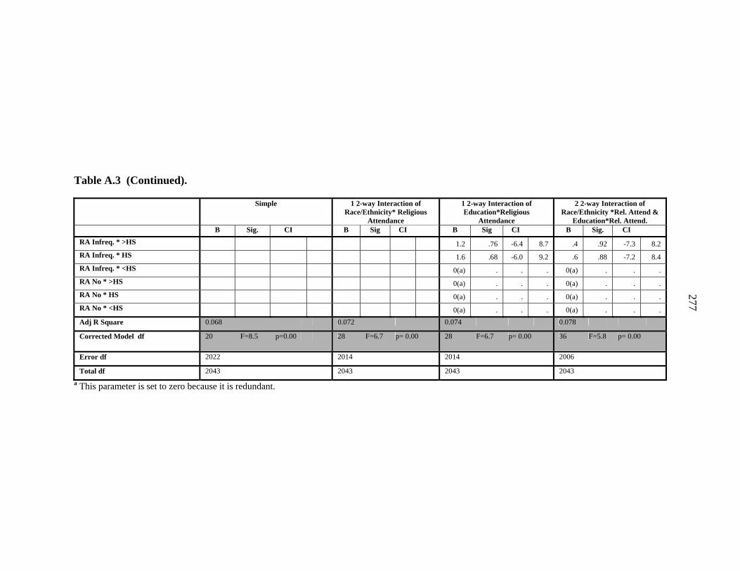
277
Table A.3 (Continued).
Simple 1 2-way Interaction of Race/Ethnicity* Religious
Attendance
1 2-way Interaction of Education*Religious
Attendance
2 2-way Interaction of Race/Ethnicity *Rel. Attend &
Education*Rel. Attend. B Sig. CI B Sig CI B Sig CI B Sig. CI RA Infreq. * >HS 1.2 .76 -6.4 8.7 .4 .92 -7.3 8.2 RA Infreq. * HS 1.6 .68 -6.0 9.2 .6 .88 -7.2 8.4 RA Infreq. * <HS 0(a) . . . 0(a) . . . RA No * >HS 0(a) . . . 0(a) . . . RA No * HS 0(a) . . . 0(a) . . . RA No * <HS 0(a) . . . 0(a) . . . Adj R Square 0.068 0.072 0.074 0.078
Corrected Model df 20 F=8.5 p=0.00 28 F=6.7 p= 0.00 28 F=6.7 p= 0.00 36 F=5.8 p= 0.00
Error df 2022 2014 2014 2006
Total df 2043 2043 2043 2043 a This parameter is set to zero because it is redundant.

278
Figure A.7 Obj. I. Model of Mental Health Composite Score (SF-12 MCS) in 2000 with the One Two-way Interaction of Religious Attendance in 2000 with Race/Ethnicity (controlling for socio-demographic variables in 2000 of gender, marital status, education, number of children living in the household, work amount in 1999, net family income in 1999, and residence).
Not at all<=Sev./yr1-3/mth1/wk>1/wk Religious Attendance 2000
55.00
54.00
53.00
52.00
51.00
Caucasian and Others
African Americans Hispanic
Race/Ethnicity
Estimated Marginal Means of Mental Health Composite Score (SF-12, MCS)2000

279
Not at all<=Sev./yr1-3/mth1/wk>1/wk
Religious Attendance 2000
56.00
54.00
52.00
50.00
48.00
46.00
44.00
Estim
ated
Mar
gina
l Mea
ns
None/GrammarHigh SchoolCollege/Grad School
Education 2000 3levels
Estimated Marginal Means of Mental Health Composite Score (SF-12, MCS)2000
Figure A.8 Obj. I. Model of Mental Health Composite Score (SF-12 MCS) in 2000 with the One Two-way Interaction of Religious Attendance in 2000 with Education in 2000 (controlling for socio-demographic variables in 2000 of gender, race/ethnicity, marital status, education, number of children living in the household, work amount in 1999, net family income in 1999, and residence).

280
Figure A.9 Obj. I. Model of Mental Health Composite Score (SF-12 MCS) in 2000 with the One Two-way Interaction of Religious Attendance in 2000 with Race/Ethnicity in 2000 (in the presence of the two-way interaction of Religious Attendance with Education in 2000; controlling for socio-demographic variables in 2000 of gender, race/ethnicity, marital status, education, number of children living in the household, work amount in 1999, net family income in 1999, and residence).
Not at all<=Sev./yr1-3/mth1/wk >1/wk Religious Attendance 2000
56.00
55.00
54.00
53.00
52.00
51.00
50.00
49.00
Est. Marginal Means
Caucasian and others
African AmericanHispanic
Race/Ethnicity
Estimated Marginal Means of Mental Health Composite Score (SF-12, MCS) 2000

281
Not at all<=Sev./yr1-3/mth1/wk>1/wk
Religious Attendance 2000
56.00
54.00
52.00
50.00
48.00
46.00
44.00
Estim
ated
Mar
gina
l Mea
ns
None/GrammarHigh SchoolCollege/Grad School
Education 2000 3levels
Estimated Marginal Means of Mental Health Composite Score (SF-12, MCS)2000
Figure A.10 Obj. I. Model of Mental Health Composite Score (SF-12 MCS) in 2000 with the One Two-way Interaction of Religious Attendance in 2000 with Education in 2000 (in the presence of the two-way interaction of religious attendance in 2000 with race/ethnicity; controlling for socio-demographic variables in 2000 of gender, race/ethnicity, marital status, education, number of children living in the household, work amount in 1999, net family income in 1999, and residence).
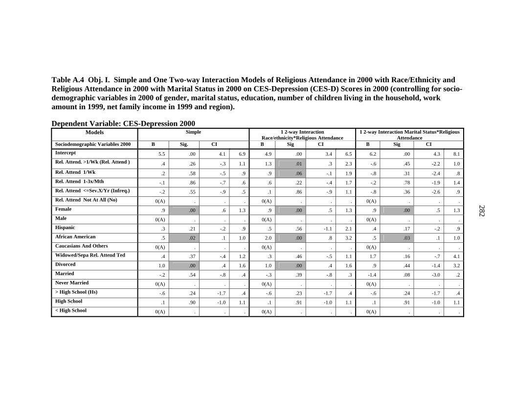
282
Table A.4 Obj. I. Simple and One Two-way Interaction Models of Religious Attendance in 2000 with Race/Ethnicity and Religious Attendance in 2000 with Marital Status in 2000 on CES-Depression (CES-D) Scores in 2000 (controlling for socio-demographic variables in 2000 of gender, marital status, education, number of children living in the household, work amount in 1999, net family income in 1999 and region).
Dependent Variable: CES-Depression 2000 Models Simple 1 2-way Interaction
Race/ethnicity*Religious Attendance 1 2-way Interaction Marital Status*Religious
Attendance Sociodemographic Variables 2000 B Sig. CI B Sig CI B Sig CI Intercept 5.5 .00 4.1 6.9 4.9 .00 3.4 6.5 6.2 .00 4.3 8.1 Rel. Attend. >1/Wk (Rel. Attend ) .4 .26 -.3 1.1 1.3 .01 .3 2.3 -.6 .45 -2.2 1.0 Rel. Attend 1/Wk .2 .58 -.5 .9 .9 .06 -.1 1.9 -.8 .31 -2.4 .8 Rel. Attend 1-3x/Mth -.1 .86 -.7 .6 .6 .22 -.4 1.7 -.2 .78 -1.9 1.4 Rel. Attend <=Sev.X/Yr (Infreq.) -.2 .55 -.9 .5 .1 .86 -.9 1.1 -.8 .36 -2.6 .9 Rel. Attend Not At All (No) 0(A) . . . 0(A) . . . 0(A) . . . Female .9 .00 .6 1.3 .9 .00 .5 1.3 .9 .00 .5 1.3 Male 0(A) . . . 0(A) . . . 0(A) . . . Hispanic .3 .21 -.2 .9 .5 .56 -1.1 2.1 .4 .17 -.2 .9 African American .5 .02 .1 1.0 2.0 .00 .8 3.2 .5 .03 .1 1.0 Caucasians And Others 0(A) . . . 0(A) . . . 0(A) . . . Widowed/Sepa Rel. Attend Ted .4 .37 -.4 1.2 .3 .46 -.5 1.1 1.7 .16 -.7 4.1 Divorced 1.0 .00 .4 1.6 1.0 .00 .4 1.6 .9 .44 -1.4 3.2 Married -.2 .54 -.8 .4 -.3 .39 -.8 .3 -1.4 .08 -3.0 .2 Never Married 0(A) . . . 0(A) . . . 0(A) . . . > High School (Hs) -.6 .24 -1.7 .4 -.6 .23 -1.7 .4 -.6 .24 -1.7 .4 High School .1 .90 -1.0 1.1 .1 .91 -1.0 1.1 .1 .91 -1.0 1.1 < High School 0(A) . . . 0(A) . . . 0(A) . . .

283
Table A.4 (Continued).
Models Simple 1 2-Way Interaction of Race/Ethnicity*Religious Attendance
1 2-Way Interaction of Marital Status*Religious Attendance
Sociodemographic Variables 2000 B Sig. Ci B Sig Ci B Sig Ci >=2 Children -.1 .59 -.6 .3 -.1 .61 -.6 .4 -.1 .59 -.6 .3 1 Child .2 .40 -.3 .8 .2 .39 -.3 .8 .2 .40 -.3 .8 No Children 0(A) . . . 0(A) . . . 0(A) . . . Work>20 Hrs/Wk (Ft) -2.0 .00 -2.5 -1.5 -2.0 .00 -2.5 -1.5 -2.0 .00 -2.5 -1.5 0-20 Hrs/Wk (Pt) 0(A) . . . 0(A) . . . 0(A) . . . Income Missing -1.0 .00 -1.7 -.4 -1.0 .00 -1.6 -.4 -1.0 .00 -1.6 -.4 Income Top 25% -2.2 .00 -2.9 -1.5 -2.1 .00 -2.8 -1.4 -2.2 .00 -2.8 -1.5 Income Mid 50% -1.8 .00 -2.4 -1.3 -1.8 .00 -2.4 -1.3 -1.8 .00 -2.3 -1.3 Income Lowest 25% 0(A) . . . 0(A) . . . 0(A) . . . Region: West .4 .21 -.2 1.0 .4 .22 -.2 1.0 .3 .29 -.3 .9 South .7 .01 .1 1.2 .7 .01 .1 1.2 .7 .02 .1 1.2 North Central. Attend L .4 .14 -.1 1.0 .5 .11 -.1 1.1 .5 .13 -.1 1.0 Northeast 0(A) . . . 0(A) . . . 0(A) . . . Rel. Attend >1/Wk * Hispanic -1.1 .25 -3.1 .8 Rel. Attend >1/Wk * African American
-2.0 .01 -3.5 -.4
Rel. Attend >1/Wk * Caucasians And Others
0(A) . . .
Rel. Attend 1/Wk * Hispanic -.5 .61 -2.3 1.4 Rel. Attend 1/Wk * African American
-1.7 .02 -3.1 -.2
Rel. Attend 1/Wk * Caucasians And Others
0(A) . . .
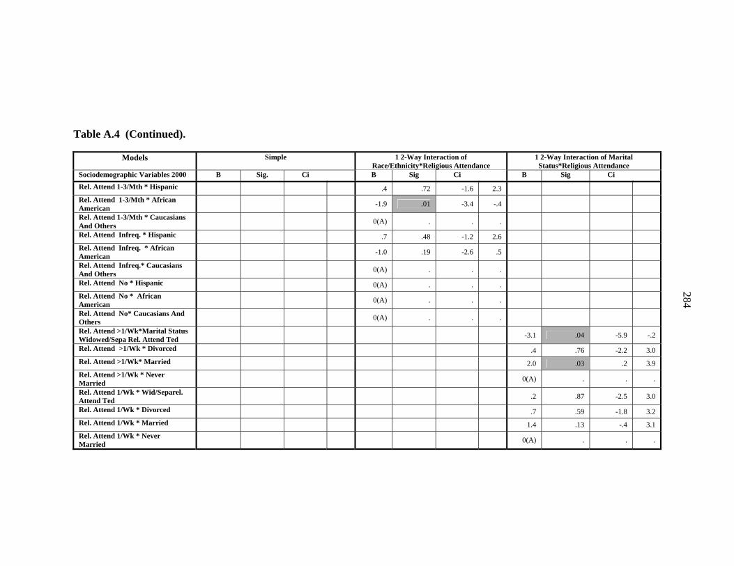
284
Table A.4 (Continued).
Models Simple 1 2-Way Interaction of Race/Ethnicity*Religious Attendance
1 2-Way Interaction of Marital Status*Religious Attendance
Sociodemographic Variables 2000 B Sig. Ci B Sig Ci B Sig Ci Rel. Attend 1-3/Mth * Hispanic .4 .72 -1.6 2.3 Rel. Attend 1-3/Mth * African American
-1.9 .01 -3.4 -.4
Rel. Attend 1-3/Mth * Caucasians And Others
0(A) . . .
Rel. Attend Infreq. * Hispanic .7 .48 -1.2 2.6 Rel. Attend Infreq. * African American
-1.0 .19 -2.6 .5
Rel. Attend Infreq.* Caucasians And Others
0(A) . . .
Rel. Attend No * Hispanic 0(A) . . . Rel. Attend No * African American
0(A) . . .
Rel. Attend No* Caucasians And Others
0(A) . . .
Rel. Attend >1/Wk*Marital Status Widowed/Sepa Rel. Attend Ted
-3.1 .04 -5.9 -.2
Rel. Attend >1/Wk * Divorced .4 .76 -2.2 3.0 Rel. Attend >1/Wk* Married 2.0 .03 .2 3.9 Rel. Attend >1/Wk * Never Married
0(A) . . .
Rel. Attend 1/Wk * Wid/Separel. Attend Ted
.2 .87 -2.5 3.0
Rel. Attend 1/Wk * Divorced .7 .59 -1.8 3.2 Rel. Attend 1/Wk * Married 1.4 .13 -.4 3.1 Rel. Attend 1/Wk * Never Married
0(A) . . .
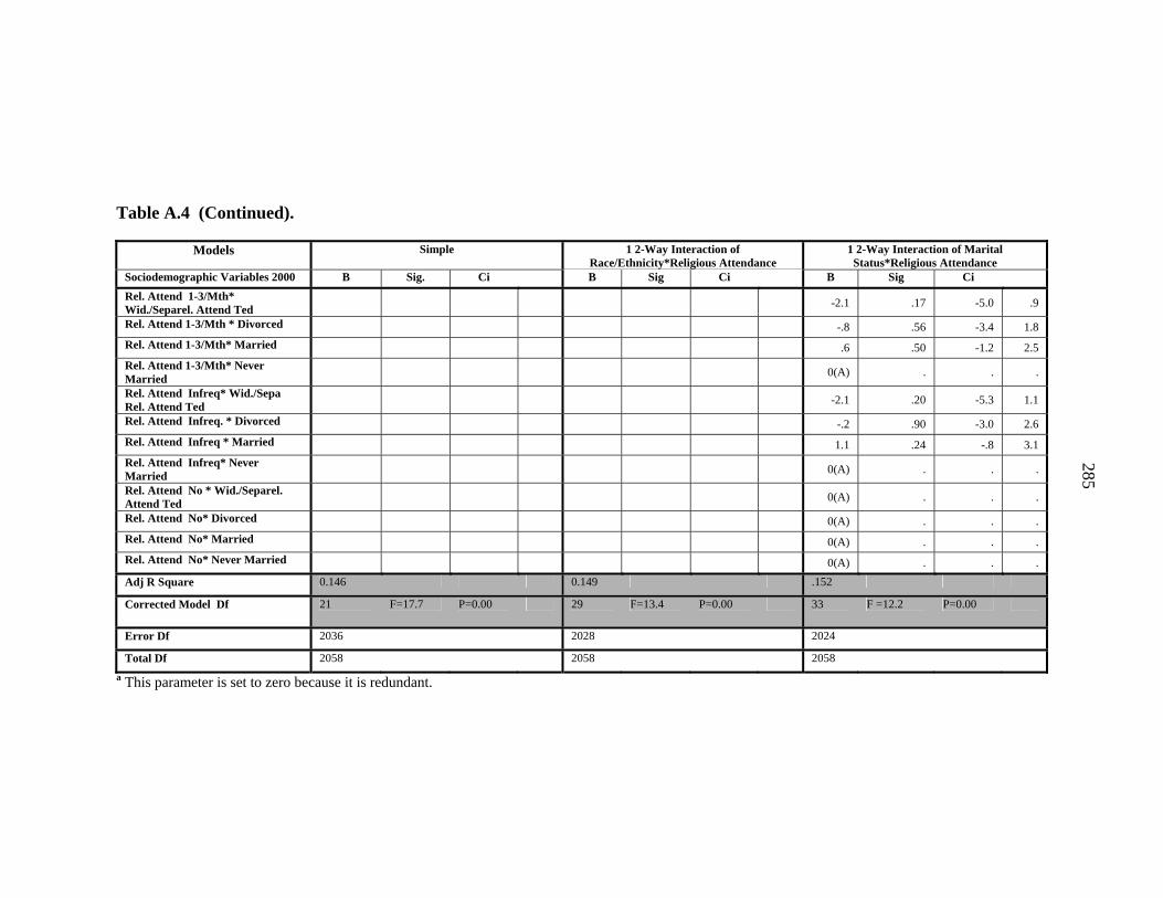
285
Table A.4 (Continued).
Models Simple 1 2-Way Interaction of Race/Ethnicity*Religious Attendance
1 2-Way Interaction of Marital Status*Religious Attendance
Sociodemographic Variables 2000 B Sig. Ci B Sig Ci B Sig Ci Rel. Attend 1-3/Mth* Wid./Separel. Attend Ted
-2.1 .17 -5.0 .9
Rel. Attend 1-3/Mth * Divorced -.8 .56 -3.4 1.8 Rel. Attend 1-3/Mth* Married .6 .50 -1.2 2.5 Rel. Attend 1-3/Mth* Never Married
0(A) . . .
Rel. Attend Infreq* Wid./Sepa Rel. Attend Ted
-2.1 .20 -5.3 1.1
Rel. Attend Infreq. * Divorced -.2 .90 -3.0 2.6 Rel. Attend Infreq * Married 1.1 .24 -.8 3.1 Rel. Attend Infreq* Never Married
0(A) . . .
Rel. Attend No * Wid./Separel. Attend Ted
0(A) . . .
Rel. Attend No* Divorced 0(A) . . . Rel. Attend No* Married 0(A) . . . Rel. Attend No* Never Married 0(A) . . .
Adj R Square 0.146 0.149 .152
Corrected Model Df 21 F=17.7 P=0.00 29 F=13.4 P=0.00 33 F =12.2 P=0.00
Error Df 2036 2028 2024
Total Df 2058 2058 2058 a This parameter is set to zero because it is redundant.

286
Figure A.11 Obj. I. Model of CES-Depression (CES-D) in 2000 with the One Two-way Interaction of Religious Attendance with Race/Ethnicity (controlling for socio-demographic variables in 2000 of gender, marital status, education, number of children living in the household, work amount in 1999, net family income in 1999 and region).
Not at all<=Sev./yr1-3/mth1/wk>1/wk Religious Attendance 2000
6.00
5.50
5.00
4.50
4.00
3.50
Estimated Marginal Means Caucasians and others
African Americans Hispanic
Race/Ethnicity
Estimated Marginal Means of CES-Depression Score

287
Not at all<=Sev./yr1-3/mth1/wk>1/wk
Religious Attendance 2000
7.00
6.00
5.00
4.00
3.00
Estim
ated
Mar
gina
l Mea
ns never marriedmarrieddivorcedwidowed/separated
marital 2000 4categories
Estimated Marginal Means of CES-Depression Score
Figure A.12 Obj. I. Obj. I. Model of CES-Depression (CES-D) in 2000 with the One Two-way Interaction of Religious Attendance with Marital Status in 2000 (controlling for socio-demographic variables in 2000 of gender, marital status, education, number of children living in the household, work amount in 1999, net family income in 1999 and region).

288
APPENDIX B Objective II

289
Table B.1 Obj.II ANOVA of the Simple Model. Physical Health, Mental Health & Depression Scores in 2000 by Religious Attendance in 1982 (controlling for sociodemographic variables in 1982 and 1998 of gender, race/ethnicity, marital status in 1982 and 1998, education in 1982, number of children living in the household in 1982 and 1998, work amount in 1981 and 1997, net family income in 1981 and 1997, residence in 1982 and 1997 and region in 1982).
Physical Health Composite Score (SF-12 PCS) 2000
Mental Health Composite Score (SF-12 MCS) 2000
CES-Depression Score (CES-D) 2000 Independent Variables 1982
Source df F Sig. df F Sig. df F Sig.
Corrected Model 30 7.0 .00 30 2.7 .00 30 7.5 .00Intercept 1 3515.9 .00 1 3971.1 .00 1 164.3 .00Religious Attendance 1982 4 .8 .51 4 2.5 .04 4 1.6 .17Health Could Limit Amt/Kind Work 1981 1 39.0 .00 1 1.8 .18 1 10.9 .00Gender 1 .9 .35 1 14.7 .00 1 5.3 .02Race/Ethnicity 2 4.0 .02 2 .3 .74 2 .6 .56Marital 1982 2 .6 .55 2 .6 .55 2 .1 .91Education 1982 1 1.6 .20 1 .1 .79 1 .0 .91Child Number Living in Household 1982 2 1.2 .31 2 1.2 .30 2 4.4 .01Work Amount 1981 1 .5 .49 1 1.1 .30 1 .1 .72Net Family Income 1981 3 .1 .98 3 .5 .65 3 .4 .77Residence 1982 1 1.5 .23 1 .4 .53 1 .9 .34Region 1982 3 .3 .80 3 1.8 .14 3 4.9 .00Marital 1998 2 5.5 .00 2 1.8 .16 2 13.8 .00Child # in Household 1998 2 1.2 .30 2 .1 .93 2 1.1 .34Work Amount 1997 1 80.1 .00 1 14.2 .00 1 51.8 .00Net Family Income 1997 3 1.0 .37 3 .8 .49 3 2.1 .09Residence 1998 1 1.0 .32 1 2.2 .14 1 1.9 .17Error 1638 1638 1643 Total 1669 1669 1674 Corrected Total 1668 1668 1673 a Adj. R Squared 0.097 0.029 0.104

290
Table B.2 Obj. II. Parameter Estimates of the Simple Model. Physical Health, Mental Health & Depression Scores in 2000 by Religious Attendance in 1982 (controlling for sociodemographic variables in 1982 and 1998 of gender, race/ethnicity, marital status in 1982 and 1998, education in 1982, number of children living in the household in 1982 and 1998, work amount in 1981 and 1997, net family income in 1981 and 1997, residence in 1982 and 1998 and region in 1982).
Physical Health Composite Score (SF-12 PCS) 2000
Mental Health Composite Score (SF-12 MCS) 2000 CES-Depression Score (CES-D) 2000 Independent Variables 1982,
1998 Parameters B Sig. CI 95% B Sig. CI 95% B Sig. CI 95%
Intercept 48.0 .00 45.1 50.9 51.9 .00 48.8 55.1 4.7 .00 3.2 6.2
Rel. Attend. 1982 >1wk (RA) .4 .63 -1.3 2.1 2.0 .04 .1 3.8 -.9 .05 -1.8 .0
Rel. Attend 1982 1/wk 1.0 .13 -.3 2.3 1.4 .04 .1 2.8 -.5 .18 -1.1 .2
Rel Attend 1982 1-3x/mth -.1 .87 -1.3 1.1 1.7 .01 .4 2.9 -.7 .03 -1.3 -.1 Rel Attend 1982<=Sev.x/yr (Infreq.) .2 .71 -.9 1.3 1.5 .01 .4 2.6 -.5 .09 -1.0 .1
Rel Attend 1982 Not at all (No) 0(a) . . . 0(a) . . . 0(a) . . .
1981 Hlh Limits Work Yes -5.6 .00 -7.4 -3.9 -1.3 .18 -3.2 .6 1.5 .00 .6 2.5
1981 Hlh Limits Work No 0(a) . . . 0(a) . . . 0(a) . . .
Female -.4 .35 -1.3 .5 -1.8 .00 -2.7 -.9 .5 .02 .1 1.0
Male 0(a) . . . 0(a) . . . 0(a) . . .
Hispanic -1.6 .01 -2.7 -.4 .5 .45 -.8 1.8 .1 .76 -.5 .7
African American -1.1 .05 -2.1 .0 .2 .67 -.9 1.4 .3 .28 -.2 .8
Caucasian and Others 0(a) . . . 0(a) . . . 0(a) . . . Marital Status 1982: Div./Wid./Sep. 1982 -1.0 .28 -2.8 .8 -.2 .81 -2.1 1.7 -.2 .74 -1.1 .8
Married 1982 -.2 .73 -1.3 .9 -.7 .28 -1.9 .5 -.1 .72 -.7 .5
Never Married 1982 0(a) . . . 0(a) . . . 0(a) . . . Education Level: >=High School 1982 1.4 .20 -.8 3.6 .3 .79 -2.0 2.6 .1 .91 -1.0 1.2
< High School 1982 0(a) . . . 0(a) . . . 0(a) . . .
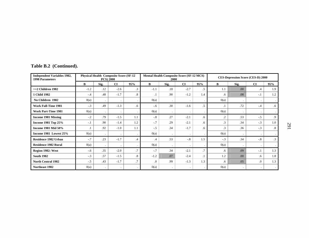
291
Table B.2 (Continued).
Physical Health Composite Score (SF-12 PCS) 2000
Mental Health Composite Score (SF-12 MCS) 2000 CES-Depression Score (CES-D) 2000 Independent Variables 1982,
1998 Parameters B Sig. CI 95% B Sig. CI 95% B Sig. CI 95%
>=2 Children 1982 -1.2 .12 -2.6 .3 -1.1 .18 -2.7 .5 1.1 .00 .4 1.9
1 Child 1982 -.4 .48 -1.7 .8 .1 .90 -1.2 1.4 .6 .08 -.1 1.2
No Children 1982 0(a) . . . 0(a) . . . 0(a) . . .
Work Full-Time 1981 -.3 .49 -1.3 .6 -.6 .30 -1.6 .5 .1 .72 -.4 .6
Work Part-Time 1981 0(a) . . . 0(a) . . . 0(a) . . .
Income 1981 Missing -.2 .79 -1.5 1.1 -.8 .27 -2.1 .6 .2 .53 -.5 .9
Income 1981 Top 25% -.1 .90 -1.4 1.2 -.7 .29 -2.1 .6 .3 .34 -.3 1.0
Income 1981 Mid 50% .1 .92 -1.0 1.1 -.5 .34 -1.7 .6 .3 .36 -.3 .8
Income 1981 Lowest 25% 0(a) . . . 0(a) . . . 0(a) . . .
Residence 1982 Urban -.7 .23 -1.7 .4 .4 .53 -.8 1.5 -.3 .34 -.8 .3
Residence 1982 Rural 0(a) . . . 0(a) . . . 0(a) . . .
Region 1982: West -.6 .35 -2.0 .7 -.7 .34 -2.1 .7 .6 .09 -.1 1.3
South 1982 -.3 .57 -1.5 .8 -1.2 .07 -2.4 .1 1.2 .00 .6 1.8
North Central 1982 -.5 .43 -1.7 .7 .0 .99 -1.3 1.3 .6 .05 .0 1.3
Northeast 1982 0(a) . . . 0(a) . . . 0(a) . . .
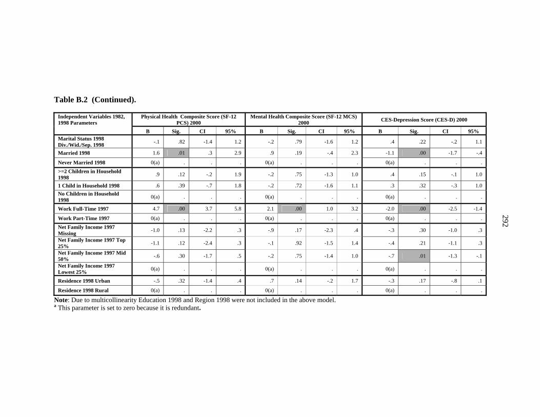
292
Table B.2 (Continued).
Physical Health Composite Score (SF-12 PCS) 2000
Mental Health Composite Score (SF-12 MCS) 2000 CES-Depression Score (CES-D) 2000 Independent Variables 1982,
1998 Parameters B Sig. CI 95% B Sig. CI 95% B Sig. CI 95%
Marital Status 1998 Div./Wid./Sep. 1998 -.1 .82 -1.4 1.2 -.2 .79 -1.6 1.2 .4 .22 -.2 1.1
Married 1998 1.6 .01 .3 2.9 .9 .19 -.4 2.3 -1.1 .00 -1.7 -.4
Never Married 1998 0(a) . . . 0(a) . . . 0(a) . . . >=2 Children in Household 1998 .9 .12 -.2 1.9 -.2 .75 -1.3 1.0 .4 .15 -.1 1.0
1 Child in Household 1998 .6 .39 -.7 1.8 -.2 .72 -1.6 1.1 .3 .32 -.3 1.0 No Children in Household 1998 0(a) . . . 0(a) . . . 0(a) . . .
Work Full-Time 1997 4.7 .00 3.7 5.8 2.1 .00 1.0 3.2 -2.0 .00 -2.5 -1.4
Work Part-Time 1997 0(a) . . . 0(a) . . . 0(a) . . . Net Family Income 1997 Missing -1.0 .13 -2.2 .3 -.9 .17 -2.3 .4 -.3 .30 -1.0 .3
Net Family Income 1997 Top 25% -1.1 .12 -2.4 .3 -.1 .92 -1.5 1.4 -.4 .21 -1.1 .3
Net Family Income 1997 Mid 50% -.6 .30 -1.7 .5 -.2 .75 -1.4 1.0 -.7 .01 -1.3 -.1
Net Family Income 1997 Lowest 25% 0(a) . . . 0(a) . . . 0(a) . . .
Residence 1998 Urban -.5 .32 -1.4 .4 .7 .14 -.2 1.7 -.3 .17 -.8 .1
Residence 1998 Rural 0(a) . . . 0(a) . . . 0(a) . . .
Note: Due to multicollinearity Education 1998 and Region 1998 were not included in the above model. a This parameter is set to zero because it is redundant.

293
Not at all<=Sev./yr1-3/mth1/wk>1/wk
Religious Attendance 1982
46.50
46.25
46.00
45.75
45.50
45.25
Estim
ated
Mar
gina
l Mea
ns
Estimated Marginal Means of Physical Health Composite Score (SF-12, PCS)2000
Figure B.1 Obj. II. Simple Model of the Physical Health Composite Score (SF-12 PCS) in 2000 by Religious Attendance in 1982 (controlling for sociodemographic variables in 1982 and 1998 of gender race/ethnicity, marital status in 1982 and 1998, education in 1982, number of children living in the household in 1982 and 1998, work amount in 1981 and 1997, net family income in 1981 and 1997, residence in 1982 and 1998 and region in 1982).
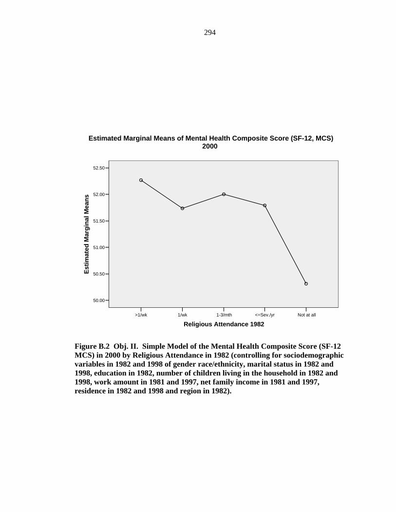
294
Not at all<=Sev./yr1-3/mth1/wk>1/wk
Religious Attendance 1982
52.50
52.00
51.50
51.00
50.50
50.00
Estim
ated
Mar
gina
l Mea
ns
Estimated Marginal Means of Mental Health Composite Score (SF-12, MCS)2000
Figure B.2 Obj. II. Simple Model of the Mental Health Composite Score (SF-12 MCS) in 2000 by Religious Attendance in 1982 (controlling for sociodemographic variables in 1982 and 1998 of gender race/ethnicity, marital status in 1982 and 1998, education in 1982, number of children living in the household in 1982 and 1998, work amount in 1981 and 1997, net family income in 1981 and 1997, residence in 1982 and 1998 and region in 1982).

295
Not at all<=Sev./yr1-3/mth1/wk>1/wk
Religious Attendance 1982
5.60
5.40
5.20
5.00
4.80
4.60
Estim
ated
Mar
gina
l Mea
ns
Estimated Marginal Means of CES-Depression Score
Figure B.3 Obj. II. Simple Model of the CES-Depression Score (CES-D) in 2000 by Religious Attendance in 1982 (controlling for sociodemographic variables in 1982 and 1998 of gender race/ethnicity, marital status in 1982 and 1998, education in 1982, number of children living in the household in 1982 and 1998, work amount in 1981 and 1997, net family income in 1981 and 1997, residence in 1982 and 1998 and region in 1982).

296
Table B.3 Obj. II. ANOVA Complete Model of Mental Health Composite Score in 2000 by One Two-way Interaction of Religious Attendance in 1982 with Race/Ethnicity, and One Two-way Interaction of Religious Attendance in 1982 with Number of Children Living in the Household in 1982, and Two Two-way Interactions of Religious Attendance in 1982 with Race/Ethnicity and Religious Attendance in 1982 with Number of Children Living in the Household in 1982 (controlling for sociodemographic variables in 1982 of gender, race/ethnicity, marital status, education, number of children living in the household, work amount in 1981, net family income in 1981, residence and region).
1 2-way Interaction Race/Ethnicity*Religious Attend
1 2-way Interaction Child #*Religious Attendance
2 2-way Interaction Race/Ethnicity*Religious Attend. and Child#*Religious Attendance
Independent Variables 1982 Source
df F Sig. df F Sig. df F Sig.
Corrected Model 29 2.7 .00 29 2.7 .00 37 2.5 .00
Intercept 1 5013.5 .00 1 4984.5 .00 1 4925.1 .00Religious Attendance (RA) 1982 4 2.0 .09 4 3.8 .00 4 2.8 .02Health Could Limit Amt/Kind Work 1981 1 2.4 .12 1 2.0 .16 1 2.2 .14Gender 1 21.5 .00 1 22.0 .00 1 21.2 .00Race/Ethnicity 2 1.1 .32 2 .7 .51 2 1.3 .27Marital 1982 2 .6 .57 2 .7 .49 2 .7 .51Education 1982 1 .0 .85 1 .0 .90 1 .0 .89Child # in Household 1982 2 2.0 .14 2 2.8 .06 2 2.9 .05Work Amount 1981 1 .4 .53 1 .2 .69 1 .2 .66Net Family Income 1981 3 1.0 .41 3 1.0 .39 3 1.0 .38Residence 1982 1 .4 .51 1 .4 .53 1 .3 .57Region 1982 3 1.0 .42 3 1.1 .36 3 .9 .45Religious Attendance1982*Race/Ethnicity 8 2.2 .02 8 2.0 .04Religious Attendance 1982*Child # 1982 8 2.3 .02 8 2.1 .03Error 1797 1797 1789 Total 1827 1827 1827 Corrected Total 1826 1826 1826 a Adj. R Squared 0.026 0.026 0.030
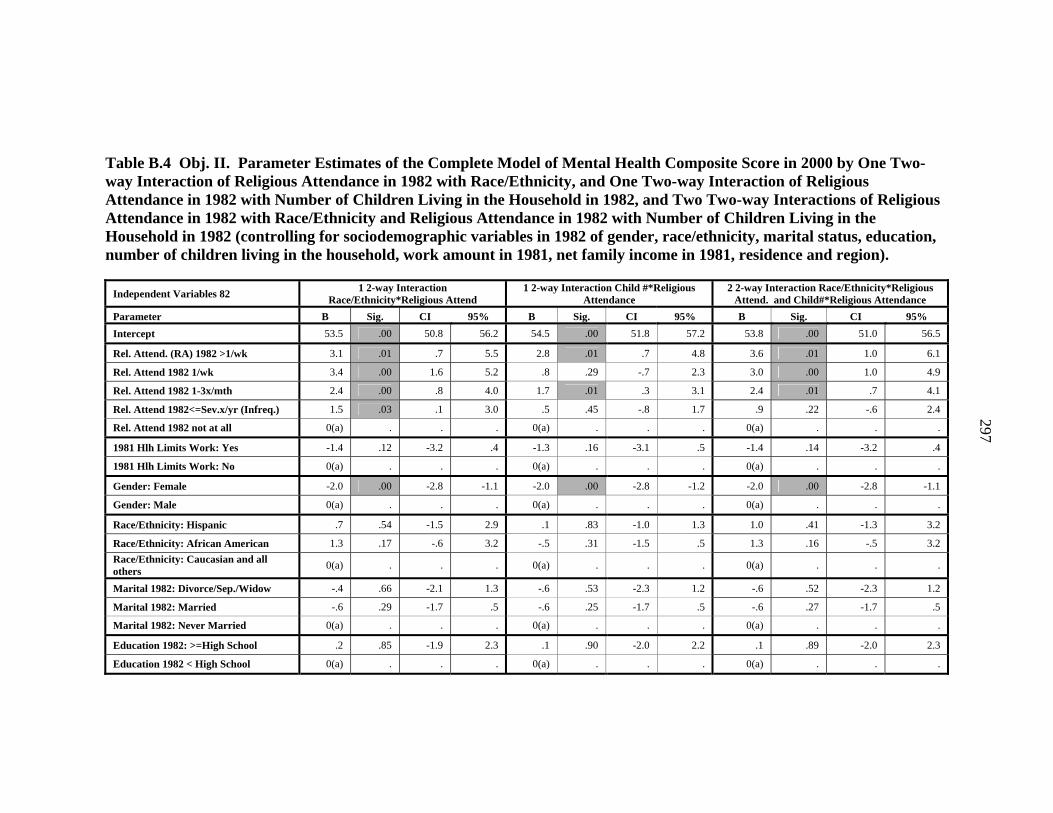
297
Table B.4 Obj. II. Parameter Estimates of the Complete Model of Mental Health Composite Score in 2000 by One Two-way Interaction of Religious Attendance in 1982 with Race/Ethnicity, and One Two-way Interaction of Religious Attendance in 1982 with Number of Children Living in the Household in 1982, and Two Two-way Interactions of Religious Attendance in 1982 with Race/Ethnicity and Religious Attendance in 1982 with Number of Children Living in the Household in 1982 (controlling for sociodemographic variables in 1982 of gender, race/ethnicity, marital status, education, number of children living in the household, work amount in 1981, net family income in 1981, residence and region).
Independent Variables 82 1 2-way Interaction Race/Ethnicity*Religious Attend
1 2-way Interaction Child #*Religious Attendance
2 2-way Interaction Race/Ethnicity*Religious Attend. and Child#*Religious Attendance
Parameter B Sig. CI 95% B Sig. CI 95% B Sig. CI 95% Intercept 53.5 .00 50.8 56.2 54.5 .00 51.8 57.2 53.8 .00 51.0 56.5
Rel. Attend. (RA) 1982 >1/wk 3.1 .01 .7 5.5 2.8 .01 .7 4.8 3.6 .01 1.0 6.1
Rel. Attend 1982 1/wk 3.4 .00 1.6 5.2 .8 .29 -.7 2.3 3.0 .00 1.0 4.9
Rel. Attend 1982 1-3x/mth 2.4 .00 .8 4.0 1.7 .01 .3 3.1 2.4 .01 .7 4.1
Rel. Attend 1982<=Sev.x/yr (Infreq.) 1.5 .03 .1 3.0 .5 .45 -.8 1.7 .9 .22 -.6 2.4
Rel. Attend 1982 not at all 0(a) . . . 0(a) . . . 0(a) . . .
1981 Hlh Limits Work: Yes -1.4 .12 -3.2 .4 -1.3 .16 -3.1 .5 -1.4 .14 -3.2 .4
1981 Hlh Limits Work: No 0(a) . . . 0(a) . . . 0(a) . . .
Gender: Female -2.0 .00 -2.8 -1.1 -2.0 .00 -2.8 -1.2 -2.0 .00 -2.8 -1.1
Gender: Male 0(a) . . . 0(a) . . . 0(a) . . .
Race/Ethnicity: Hispanic .7 .54 -1.5 2.9 .1 .83 -1.0 1.3 1.0 .41 -1.3 3.2
Race/Ethnicity: African American 1.3 .17 -.6 3.2 -.5 .31 -1.5 .5 1.3 .16 -.5 3.2 Race/Ethnicity: Caucasian and all others 0(a) . . . 0(a) . . . 0(a) . . .
Marital 1982: Divorce/Sep./Widow -.4 .66 -2.1 1.3 -.6 .53 -2.3 1.2 -.6 .52 -2.3 1.2
Marital 1982: Married -.6 .29 -1.7 .5 -.6 .25 -1.7 .5 -.6 .27 -1.7 .5
Marital 1982: Never Married 0(a) . . . 0(a) . . . 0(a) . . .
Education 1982: >=High School .2 .85 -1.9 2.3 .1 .90 -2.0 2.2 .1 .89 -2.0 2.3
Education 1982 < High School 0(a) . . . 0(a) . . . 0(a) . . .

298
Table B.4 (Continued).
Independent Variables 82 1 2-way Interaction Race/Ethnicity*Religious Attend
1 2-way Interaction Child #*Religious Attendance
2 2-way Interaction Race/Ethnicity*Religious Attend. and Child#*Religious Attendance
Parameter B Sig. CI 95% B Sig. CI 95% B Sig. CI 95% Children # in Household 1982: >=2 -1.4 .06 -2.9 .1 -3.0 .04 -5.8 -.1 -3.2 .03 -6.0 -.3
Children # in Household 1982 = 1 .0 .96 -1.3 1.2 -.8 .49 -3.0 1.5 -.8 .50 -3.0 1.5
Children # in Household 1982 = 0 0(a) . . . 0(a) . . . 0(a) . . .
Work Full-Time 1981 -.3 .53 -1.3 .7 -.2 .69 -1.2 .8 -.2 .66 -1.2 .8
Work Part-Time 1981 0(a) . . . 0(a) . . . 0(a) . . .
Net Family Income 1981 Missing -.9 .18 -2.2 .4 -1.0 .14 -2.3 .3 -.9 .16 -2.2 .4
Net Family Income 1981 Top 25% -1.0 .12 -2.3 .3 -1.0 .13 -2.3 .3 -1.0 .12 -2.3 .3
Net Family Income 1981 Mid 50% -.6 .30 -1.6 .5 -.6 .25 -1.7 .4 -.6 .28 -1.6 .5
Net Family Income 1981 Lowest 25% 0(a) . . . 0(a) . . . 0(a) . . .
Residence 1982: Rural .4 .51 -.7 1.4 .3 .53 -.7 1.4 .3 .57 -.7 1.4
Residence 1982:Urban 0(a) . . . 0(a) . . . 0(a) . . .
Region 1982: West -.2 .71 -1.6 1.1 -.4 .58 -1.7 1.0 -.3 .66 -1.6 1.0
Region 1982: South -.6 .33 -1.8 .6 -.7 .24 -1.9 .5 -.6 .31 -1.8 .6
Region 1982: North Central .3 .65 -.9 1.5 .2 .77 -1.0 1.4 .2 .73 -1.0 1.4
Region 1982: Northeast 0(a) . . . 0(a) . . . 0(a) . . .

299
Table B.4 (Continued).
Independent Variables 82 1 2-way Interaction Race/Ethnicity*Religious Attend
1 2-way Interaction Child #*Religious Attendance
2 2-way Interaction Race/Ethnicity*Religious Attend. and Child#*Religious Attendance
Parameter B Sig. CI 95% B Sig. CI 95% B Sig. CI 95% Rel. Attend 1982 >1/Wk* Hispanic -1.4 .54 -5.7 3.0 -1.1 .61 -5.6 3.3 Rel. Attend 1982 >1/Wk* African American -2.6 .21 -6.6 1.5 -2.4 .25 -6.4 1.7
Rel. Attend 1982 >1/Wk*Caucasian 0(a) . . . 0(a) . . . Rel. Attend 1982 1/Wk*Hispanic -2.6 .14 -6.0 .9 -2.9 .10 -6.4 .5 Rel. Attend 1982 1/Wk* African American -5.5 .00 -8.5 -2.5 -5.5 .00 -8.5 -2.5
Rel. Attend 1982 1/Wk* Caucasian 0(a) . . . 0(a) . . . Rel. Attend 1982 1-3/Mth* Hispanic .0 .98 -3.3 3.2 -.1 .94 -3.4 3.2 Rel. Attend 1982 1-3/Mth* African American -2.5 .06 -5.1 .1 -2.4 .07 -5.0 .2
Rel. Attend 1982 1-3/Mth*Caucasian 0(a) . . . 0(a) . . . Rel. Attend 1982 Infreq * Hispanic -.3 .86 -3.2 2.7 -.9 .55 -3.8 2.1 Rel. Attend 1982 Infreq * African American -.3 .80 -2.8 2.2 -.9 .48 -3.4 1.6
Rel. Attend 1982 Infreq.* Caucasian 0(a) . . . 0(a) . . . Rel. Attend 1982 None* Hispanic 0(a) . . . 0(a) . . . Rel. Attend 1982 None * African American 0(a) . . . 0(a) . . .
Rel. Attend 1982 None* Caucasian 0(a) . . . 0(a) . . .
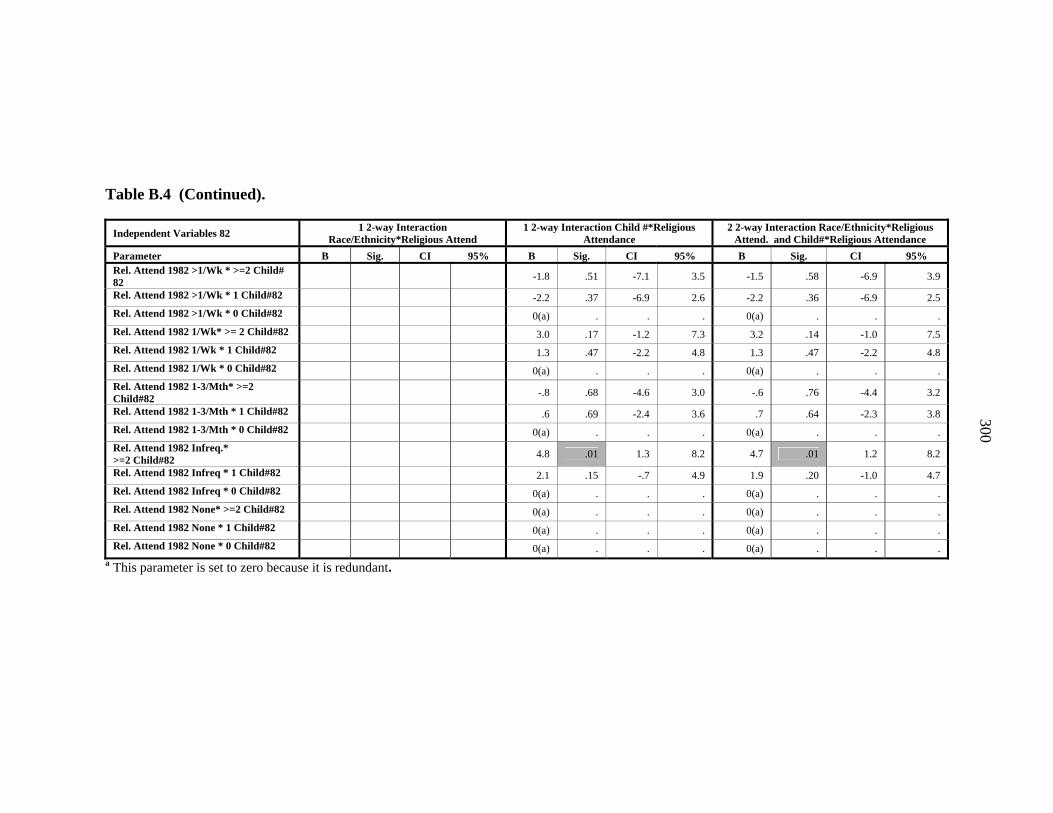
300
Table B.4 (Continued).
Independent Variables 82 1 2-way Interaction Race/Ethnicity*Religious Attend
1 2-way Interaction Child #*Religious Attendance
2 2-way Interaction Race/Ethnicity*Religious Attend. and Child#*Religious Attendance
Parameter B Sig. CI 95% B Sig. CI 95% B Sig. CI 95% Rel. Attend 1982 >1/Wk * >=2 Child# 82 -1.8 .51 -7.1 3.5 -1.5 .58 -6.9 3.9
Rel. Attend 1982 >1/Wk * 1 Child#82 -2.2 .37 -6.9 2.6 -2.2 .36 -6.9 2.5 Rel. Attend 1982 >1/Wk * 0 Child#82 0(a) . . . 0(a) . . . Rel. Attend 1982 1/Wk* >= 2 Child#82 3.0 .17 -1.2 7.3 3.2 .14 -1.0 7.5 Rel. Attend 1982 1/Wk * 1 Child#82 1.3 .47 -2.2 4.8 1.3 .47 -2.2 4.8 Rel. Attend 1982 1/Wk * 0 Child#82 0(a) . . . 0(a) . . . Rel. Attend 1982 1-3/Mth* >=2 Child#82 -.8 .68 -4.6 3.0 -.6 .76 -4.4 3.2
Rel. Attend 1982 1-3/Mth * 1 Child#82 .6 .69 -2.4 3.6 .7 .64 -2.3 3.8 Rel. Attend 1982 1-3/Mth * 0 Child#82 0(a) . . . 0(a) . . . Rel. Attend 1982 Infreq.* >=2 Child#82 4.8 .01 1.3 8.2 4.7 .01 1.2 8.2
Rel. Attend 1982 Infreq * 1 Child#82 2.1 .15 -.7 4.9 1.9 .20 -1.0 4.7 Rel. Attend 1982 Infreq * 0 Child#82 0(a) . . . 0(a) . . . Rel. Attend 1982 None* >=2 Child#82 0(a) . . . 0(a) . . . Rel. Attend 1982 None * 1 Child#82 0(a) . . . 0(a) . . . Rel. Attend 1982 None * 0 Child#82 0(a) . . . 0(a) . . .
a This parameter is set to zero because it is redundant.
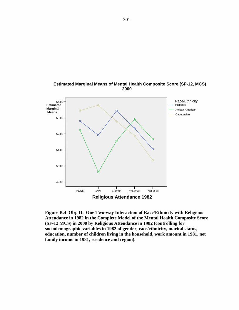
301
Figure B.4 Obj. II. One Two-way Interaction of Race/Ethnicity with Religious Attendance in 1982 in the Complete Model of the Mental Health Composite Score (SF-12 MCS) in 2000 by Religious Attendance in 1982 (controlling for sociodemographic variables in 1982 of gender, race/ethnicity, marital status, education, number of children living in the household, work amount in 1981, net family income in 1981, residence and region).
Not at all<=Sev./yr1-3/mth1/wk>1/wk
Religious Attendance 1982
54.00
53.00
52.00
51.00
50.00
49.00
Estimated Marginal Means
Cacucasian
African American
HispanicRace/Ethnicity
Estimated Marginal Means of Mental Health Composite Score (SF-12, MCS)2000

302
Not at all<=Sev./yr1-3/mth1/wk>1/wk
Religious Attendance 1982
55.00
54.00
53.00
52.00
51.00
50.00
49.00
48.00
Estim
ated
Mar
gina
l Mea
ns
0 Children1 Child>= 2 Children
Children 82 # 3 cat
Estimated Marginal Means of Mental Health Composite Score (SF-12, MCS)2000
Figure B.5 Obj. II. One Two-way Interaction of Number of Children Living in the Household in 1982 with Religious Attendance in 1982 in the Complete Model of Mental Health Composite Score (SF-12 MCS) in 2000 by Religious Attendance in 1982 (controlling for sociodemographic variables in 1982 of gender, race/ethnicity, marital status, education, number of children living in the household, work amount in 1981, net family income in 1981, residence and region).

303
Figure B.6 Obj. II. One Two-way Interaction of Race/Ethnicity with Religious Attendance in 1982 in the Presence of the One Two-Way Interaction of Number of Children Living in the Household in 1982 by Religious Attendance in 1982 in the Complete Model of Mental Health Composite Score (SF-12 MCS) in 2000 by Religious Attendance in 1982 (controlling for sociodemographic variables in 1982 of gender, race/ethnicity, marital status, education, number of children living in the household, work amount in 1981, net family income in 1981, residence and region).
Not at all<=Sev./yr1-3/mth1/wk>1/wk
Religious Attendance 1982
56.00
54.00
52.00
50.00
48.00
Estimated Marginal Means
Caucasian African American
Hispanic Race/Ethnicity
Estimated Marginal Means of Mental Health Composite Score (SF-12, MCS)2000

304
Not at all<=Sev./yr1-3/mth1/wk>1/wk
Religious Attendance 1982
56.00
54.00
52.00
50.00
48.00
Estim
ated
Mar
gina
l Mea
ns
0 Children1 Child>= 2 Children
Children 82 # 3 cat
Estimated Marginal Means of Mental Health Composite Score (SF-12, MCS)2000
Figure B.7 Obj. II. One Two-way Interaction of Number of Children Living in the Household in 1982 with Religious Attendance in 1982 in the Presence of the One Two-way interaction of Race/Ethnicity with Religious Attendance in 1982 in the Complete Model of Mental Health Composite Score (SF-12 MCS) in 2000 by Religious Attendance in 1982 (controlling for sociodemographic variables in 1982 of gender, race/ethnicity, marital status, education, number of children living in the household, work amount in 1981, net family income in 1981, residence and region).

305
Table B.5 Obj. II. ANOVA of the Complete Model of CES-Depression Score in 2000 by One Two-way Interaction of Religious Attendance in 1982 with Race/Ethnicity, and Religious Attendance in 1982 with Number of Children Living in the Household in 1982; and Two Two-way Interactions of Religious Attendance in 1982 with Race/Ethnicity and Religious Attendance in 1982 with Number of Children Living in the Household in 1982 (controlling for sociodemographic variables in 1982 of gender, race/ethnicity, marital status, education, number of children living in the household, work amount in 1981, net family income in 1981, residence and region).
1 2-way Interaction Race/Ethnicity*Religious Attend
1 2-way Interaction Child #*Religious Attendance
2 2-way Interaction Race/Ethnicity*Religious Attend. and Child#*Religious Attendance Independent Variables 1982
Source df F Sig. df F Sig. df F Sig.
Corrected Model 29 5.1 .00 29 5.0 .00 37 4.5 .00
Intercept 1 165.9 .00 1 172.4 .00 1 173.7 .00Religious Attendance (RA) 1982 4 1.0 .43 4 1.9 .11 4 1.1 .33Health Could Limit Amt/Kind Work 1981 1 17.4 .00 1 15.8 .00 1 17.0 .00Gender 1 13.5 .00 1 13.7 .00 1 13.3 .00Race/Ethnicity 2 10.0 .00 2 6.8 .00 2 9.4 .00Marital 1982 2 .4 .65 2 .2 .80 2 .3 .74Education 1982 1 .1 .73 1 .2 .66 1 .1 .73Child # in Household 1982 2 8.2 .00 2 9.8 .00 2 10.4 .00Work Amount 1981 1 .7 .41 1 1.3 .26 1 1.2 .27Net Family Income 1981 3 1.0 .40 3 .9 .43 3 1.1 .36Residence 1982 1 .4 .50 1 .5 .50 1 .5 .49Region 1982 3 2.5 .05 3 3.2 .02 3 2.8 .04RA82*Race/Ethnicity 8 2.9 .00 8 2.4 .01RA82*Child#82 8 2.7 .01 8 2.2 .02Error 1803 1803 1795 4.5 .00Total 1833 1833 1833 173.7 .00Corrected Total 1832 1832 1832 1.1 .33a Adj. R Squared 0.061 0.060 0.066

306
Table B.6 Obj.II. Parameter Estimates of the Complete Model CES-Depression Score in 2000 by One Two-way Interaction of Religious Attendance in 1982 with Race/Ethnicity, and Religious Attendance in 1982 with Number of Children Living in the Household in 1982; and Two Two-way Interactions of Religious Attendance with Race/Ethnicity, and Religious Attendance in 1982 with Number of Children Living in the Household in 1982 (controlling for sociodemographic variables in 1982 of gender, race/ethnicity, marital status, education, number of children living in the household, work amount in 1981, net family income in 1981, residence and region).
Independent Variables 82 1 2-way Interaction Race/Ethnicity*Religious Attend
1 2-way Interaction Child #*Religious Attendance
2 2-way Interaction Race/Ethnicity*Religious Attend. and Child#*Religious Attendance
Parameter B Sig. CI 95% B Sig. CI 95% B Sig. CI 95% Intercept 2.7 .00 1.3 4.0 2.4 .00 1.1 3.8 2.7 .00 1.4 4.1
Rel. Attend. 1982 >1/wk (RA) -2.0 .00 -3.2 -.8 -1.7 .00 -2.7 -.7 -2.4 .00 -3.7 -1.2
Rel. Attend 1982 1/wk -1.4 .00 -2.3 -.5 -.4 .31 -1.2 .4 -1.2 .01 -2.2 -.3
Rel. Attend 1982 1-3x/mth -1.3 .00 -2.1 -.5 -1.0 .00 -1.7 -.3 -1.5 .00 -2.3 -.6
Rel. Attend 1982<=Sev.x/yr (Infreq.) -.6 .11 -1.3 .1 -.3 .30 -1.0 .3 -.5 .21 -1.2 .3
Rel. Attend 1982 not at all 0(a) . . . 0(a) . . . 0(a) . . .
81 Hlh Limits Work: Yes 1.9 .00 1.0 2.8 1.8 .00 .9 2.7 1.9 .00 1.0 2.8
81 Hlh Limits Work: No 0(a) . . . 0(a) . . . 0(a) . . .
Gender: Female .8 .00 .4 1.2 .8 .00 .4 1.2 .8 .00 .4 1.2
Gender: Male 0(a) . . . 0(a) . . . 0(a) . . .
Race/Ethnicity: Hispanic -.5 .34 -1.7 .6 .4 .23 -.2 .9 -.6 .33 -1.7 .6
Race/Ethnicity: African American .3 .48 -.6 1.3 .9 .00 .4 1.4 .3 .52 -.6 1.3 Race/Ethnicity: Caucasian and all others 0(a) . . . 0(a) . . . 0(a) . . .
Marital 1982: Divorce/Sep./Widow -.2 .63 -1.1 .7 -.1 .78 -1.0 .7 -.1 .78 -1.0 .7
Marital 1982: Married -.3 .37 -.8 .3 -.2 .51 -.7 .4 -.2 .44 -.8 .3
Marital 1982: Never Married 0(a) . . . 0(a) . . . 0(a) . . .
Education 1982: >=High School -.2 .73 -1.2 .9 -.2 .66 -1.3 .8 -.2 .73 -1.2 .9
Education 1982 < High School 0(a) . . . 0(a) . . . 0(a) . . .

307
Table B.6 (Continued).
Independent Variables 82 1 2-way Interaction Race/Ethnicity*Religious Attend
1 2-way Interaction Child #*Religious Attendance
2 2-way Interaction Race/Ethnicity*Religious Attend. and Child#*Religious Attendance
Parameter B Sig. CI 95% B Sig. CI 95% B Sig. CI 95% Children # 1982: >=2 1.4 .00 .7 2.2 1.5 .03 .1 3.0 1.7 .02 .3 3.1
Children # 1982 = 1 .9 .01 .2 1.5 .5 .40 -.6 1.6 .6 .33 -.6 1.7
Children # 1982 = 0 0(a) . . . 0(a) . . . 0(a) . . .
Work Full-Time 1981 -.2 .41 -.7 .3 -.3 .26 -.8 .2 -.3 .27 -.8 .2
Work Part-Time 1981 0(a) . . . 0(a) . . . 0(a) . . .
Net Family Income 1981 Missing .4 .23 -.2 1.0 .4 .20 -.2 1.1 .4 .19 -.2 1.1
Net Family Income 1981 Top 25% .5 .10 -.1 1.2 .5 .13 -.1 1.1 .5 .09 -.1 1.2
Net Family Income 1981 Mid 50% .3 .23 -.2 .9 .3 .21 -.2 .9 .3 .21 -.2 .9
Net Family Income 1981 Lowest 25% 0(a) . . . 0(a) . . . 0(a) . . .
Residence 1982: Rural -.2 .50 -.7 .3 -.2 .50 -.7 .3 -.2 .49 -.7 .3
Residence 1982:Urban 0(a) . . . 0(a) . . . 0(a) . . .
Region 1982: West .5 .15 -.2 1.2 .6 .10 -.1 1.2 .5 .13 -.1 1.2
Region 1982: South .8 .01 .2 1.4 .9 .00 .3 1.5 .9 .00 .3 1.5
Region 1982: North Central .6 .06 .0 1.2 .6 .05 .0 1.2 .6 .05 .0 1.2
Region 1982: Northeast 0(a) . . . 0(a) . . . 0(a) . . .

308
Table B.6 (Continued).
Independent Variables 82 1 2-way Interaction Race/Ethnicity*Religious Attend
1 2-way Interaction Child #*Religious Attendance
2 2-way Interaction Race/Ethnicity*Religious Attend. and Child#*Religious Attendance
Parameter B Sig. CI 95% B Sig. CI 95% B Sig. CI 95% Rel. Attend 1982 >1/Wk* Hispanic 2.0 .07 -.2 4.1 1.6 .16 -.6 3.8 Rel. Attend 1982 >1/Wk* African American 1.9 .06 -.1 3.9 1.7 .09 -.3 3.7
Rel. Attend 1982 >1/Wk*Caucasian 0(A) . . . 0(A) . . . Rel. Attend 1982 1/Wk*Hispanic 1.4 .11 -.3 3.1 1.5 .09 -.2 3.2 Rel. Attend 1982 1/Wk* African American 2.1 .01 .6 3.6 2.1 .01 .6 3.6
Rel. Attend 1982 1/Wk* Caucasian 0(A) . . . 0(A) . . . Rel. Attend 1982 1-3/Mth* Hispanic 1.1 .18 -.5 2.7 1.0 .23 -.6 2.6 Rel. Attend 1982 1-3/Mth* African American 1.2 .06 -.1 2.5 1.1 .08 -.2 2.4
Rel. Attend 1982 1-3/Mth*Caucasian 0(A) . . . 0(A) . . . Rel. Attend 1982 Infreq * Hispanic 1.0 .16 -.4 2.5 1.2 .12 -.3 2.6 Rel. Attend 1982 Infreq * African American -.6 .37 -1.8 .7 -.4 .57 -1.6 .9
Rel. Attend 1982 Infreq.* Caucasian 0(A) . . . 0(A) . . . Rel. Attend 1982 None* Hispanic 0(A) . . . 0(A) . . . Rel. Attend 1982 None * African American 0(A) . . . 0(A) . . .
Rel. Attend 1982 None* Caucasian 0(A) . . . 0(A) . . .
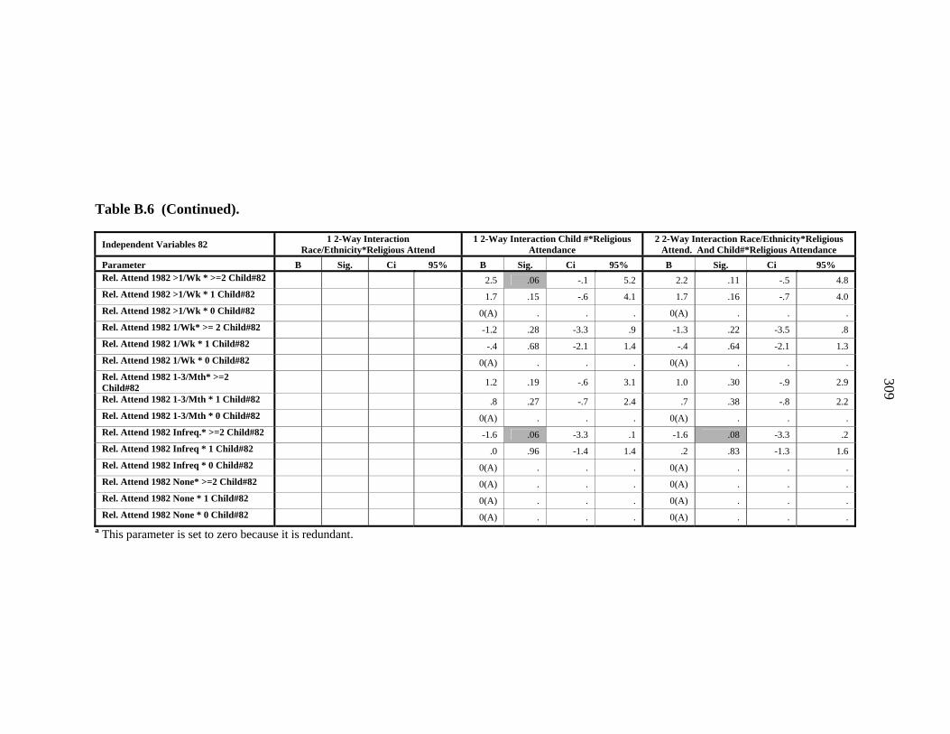
309
Table B.6 (Continued).
Independent Variables 82 1 2-Way Interaction Race/Ethnicity*Religious Attend
1 2-Way Interaction Child #*Religious Attendance
2 2-Way Interaction Race/Ethnicity*Religious Attend. And Child#*Religious Attendance
Parameter B Sig. Ci 95% B Sig. Ci 95% B Sig. Ci 95% Rel. Attend 1982 >1/Wk * >=2 Child#82 2.5 .06 -.1 5.2 2.2 .11 -.5 4.8 Rel. Attend 1982 >1/Wk * 1 Child#82 1.7 .15 -.6 4.1 1.7 .16 -.7 4.0 Rel. Attend 1982 >1/Wk * 0 Child#82 0(A) . . . 0(A) . . . Rel. Attend 1982 1/Wk* >= 2 Child#82 -1.2 .28 -3.3 .9 -1.3 .22 -3.5 .8 Rel. Attend 1982 1/Wk * 1 Child#82 -.4 .68 -2.1 1.4 -.4 .64 -2.1 1.3 Rel. Attend 1982 1/Wk * 0 Child#82 0(A) . . . 0(A) . . . Rel. Attend 1982 1-3/Mth* >=2 Child#82 1.2 .19 -.6 3.1 1.0 .30 -.9 2.9
Rel. Attend 1982 1-3/Mth * 1 Child#82 .8 .27 -.7 2.4 .7 .38 -.8 2.2 Rel. Attend 1982 1-3/Mth * 0 Child#82 0(A) . . . 0(A) . . . Rel. Attend 1982 Infreq.* >=2 Child#82 -1.6 .06 -3.3 .1 -1.6 .08 -3.3 .2 Rel. Attend 1982 Infreq * 1 Child#82 .0 .96 -1.4 1.4 .2 .83 -1.3 1.6 Rel. Attend 1982 Infreq * 0 Child#82 0(A) . . . 0(A) . . . Rel. Attend 1982 None* >=2 Child#82 0(A) . . . 0(A) . . . Rel. Attend 1982 None * 1 Child#82 0(A) . . . 0(A) . . . Rel. Attend 1982 None * 0 Child#82 0(A) . . . 0(A) . . .
a This parameter is set to zero because it is redundant.

310
Figure B.8 Obj. II. CES-Depression (CES-D) Score in 2000 by One Two-way Interaction of Religious Attendance in 1982 with Race/Ethnicity (controlling for sociodemographic variables in 1982 of gender, race/ethnicity, marital status, education, number of children living in the household, work amount in 1981, net family income in 1981, residence and region).
Not at all<=Sev./yr1-3/mth1/wk>1/wk Religious Attendance 1982
6.00
5.00
4.00
3.00
Estimated Marginal Means
Caucasian
African American Hispanic
Race/Ethnicity
Estimated Marginal Means of CES-Depression Score

311
Not at all<=Sev./yr1-3/mth1/wk>1/wk
Religious Attendance 1982
7.00
6.00
5.00
4.00
3.00
2.00
Estim
ated
Mar
gina
l Mea
ns
0 Children1 Child>= 2 Children
Children 82 # 3 cat
Estimated Marginal Means of CES-Depression Score
Figure B.9 Obj. II. CES-Depression (CES-D) Scores in 2000 by One Two-way Interaction of Religious Attendance in 1982 with Number of Children Living in the Household (controlling for sociodemographic variables in 1982 of gender, race/ethnicity, marital status, education, number of children living in the household, work amount in 1981, net family income in 1981, residence and region).
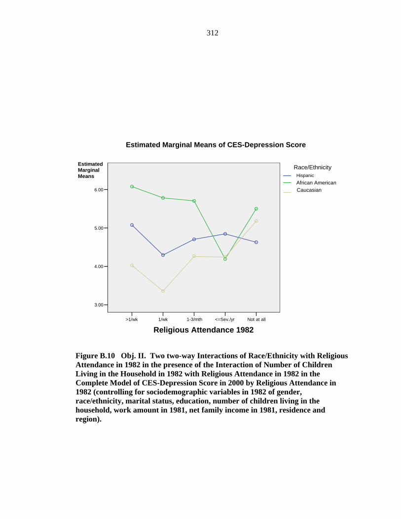
312
Figure B.10 Obj. II. Two two-way Interactions of Race/Ethnicity with Religious Attendance in 1982 in the presence of the Interaction of Number of Children Living in the Household in 1982 with Religious Attendance in 1982 in the Complete Model of CES-Depression Score in 2000 by Religious Attendance in 1982 (controlling for sociodemographic variables in 1982 of gender, race/ethnicity, marital status, education, number of children living in the household, work amount in 1981, net family income in 1981, residence and region).
Not at all<=Sev./yr1-3/mth1/wk>1/wk Religious Attendance 1982
6.00
5.00
4.00
3.00
Caucasian
African American Hispanic
Race/Ethnicity
Estimated Marginal Means of CES-Depression Score
Estimated Marginal Means
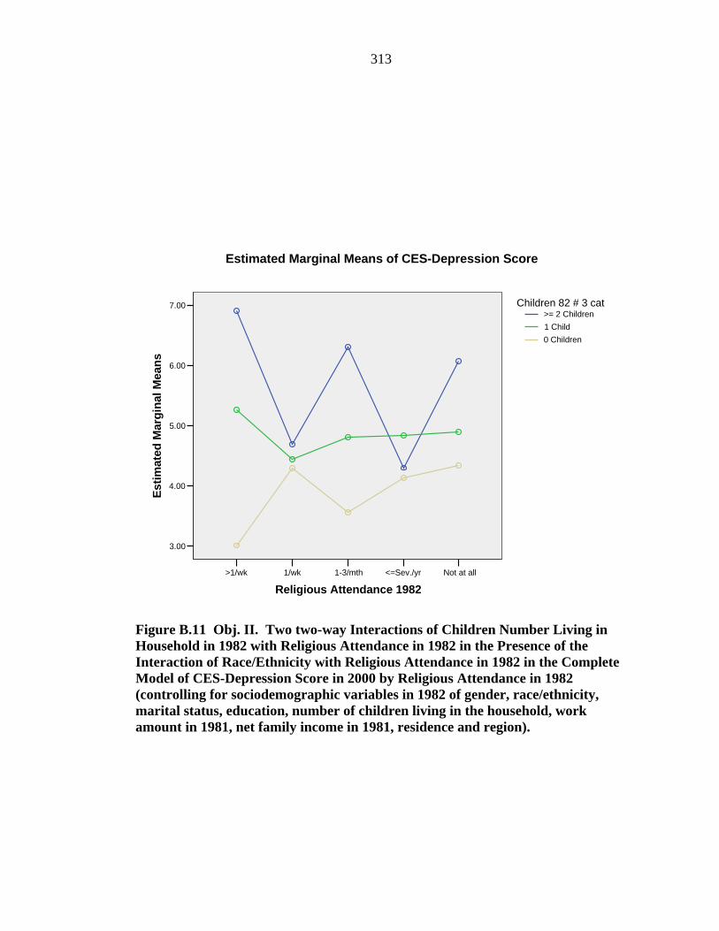
313
Not at all<=Sev./yr1-3/mth1/wk>1/wk
Religious Attendance 1982
7.00
6.00
5.00
4.00
3.00
Estim
ated
Mar
gina
l Mea
ns
0 Children1 Child>= 2 Children
Children 82 # 3 cat
Estimated Marginal Means of CES-Depression Score
Figure B.11 Obj. II. Two two-way Interactions of Children Number Living in Household in 1982 with Religious Attendance in 1982 in the Presence of the Interaction of Race/Ethnicity with Religious Attendance in 1982 in the Complete Model of CES-Depression Score in 2000 by Religious Attendance in 1982 (controlling for sociodemographic variables in 1982 of gender, race/ethnicity, marital status, education, number of children living in the household, work amount in 1981, net family income in 1981, residence and region).

314
APPENDIX C Quantitative Results
Objective III

315
Beliefs and Health Study
Consent Form
You are invited to participate in a research study on the relationship between socio-
cultural beliefs (particularly religious, spiritual, local or personal belief systems) and
health. You were selected as a possible participant because of your professional or
personal experience. We ask that you read this form and ask any questions you may
have before agreeing to be in the study.
Background Information: The purpose of this study is to obtain the most current
information from an international perspective on the effects of socio-cultural beliefs
(particularly those that belong to religious, spiritual, local or personal belief systems)
on health.
Procedures: If you agree to be in this study, we will ask you to be an interviewee and
respond to a series of inquiries related to the topic of beliefs and health. The interview
will range from a minimum of 30 minutes to a maximum of 60 minutes. The interview
is expected to occur once and if necessary a follow-up interview or interviews (in
person, by phone or by e-mail) will be requested for additional information or
clarification of initial responses.
Risks and Benefits of Participation in the Study: I do not anticipate that any risks
will arise from your participation in this study, other than those encountered in day-to-
day life. There are no direct benefits from participating in the study. Indirect benefits
from participation may be found in your contributing timely information to the body
of knowledge pertaining to emerging themes and concepts that frame the relationship

316
between beliefs and health from an international perspective or from your contribution
to our understanding of the most current humanitarian and health projects with a
socio-cultural belief component.
Voluntary Nature of Participation: Your decision whether or not to participate will
not affect your current or future relations with Cornell University or with other
cooperating entities. If you decide to participate, you are free to withdraw at any time
without affecting those relationships. You may also skip any questions in responding
to which you do not feel comfortable.
Confidentiality: The records of this study will be kept private. In any sort of report
we may publish or present, if you request, we will not include any information that
will make it possible to identify you (refer to signature request below). Research
records, tape recordings and photographs will be kept in a locked cabinet file and
computer file located in a secured locked room; only the researcher and dissertation
committee of four faculty members will have access to the records. The records, tapes
and any other material may be kept in perpetuity.
Contacts and Questions: The researcher conducting this study is Jennifer A. Nolan,
Ph.D. candidate in the department of Policy Analysis and Management, College of
Human Ecology at Cornell University. Please ask any questions you have now. If you
have questions later, you may contact me at any time at e-mail address__________. E-
mail is the best way to contact me. During the interview period, I will have access to a
cell phone. You can attempt to contact me or leave a voice message at the following
phone number: ________. and postal mailing address _____________. (I can be
contacted at the e-mail address at any time, and at the phone and mailing address

317
between ________and _________.) My dissertation chair advisor is Eunice Rodriguez
(e-mail:__________; phone number: __________; and postal mailing address:
______________). If you have any questions or concerns regarding your rights as a
subject in this study, you may contact the University Committee on Human Subjects
(UCHS) of Cornell University at __________, or access their website at
http://www.osp.cornell.edu/Compliance/UCHS/homepageUCHS.htm.
You will be given a copy of this form to keep for your records.
For each statement below, please check the appropriate response and sign and date.
Statement of Consent: I have read the above information, and have received answers
to any questions I asked. I consent to participate in the study.
Signature ________________________________ Date ________________________
Statement of Consent for Audio taping Interview: I have read the above
information. I consent to being audio taped for this study. Please check appropriate
response and sign and date.
Signature_________________________________ Date ________________________

318
Statement of Consent for Use of Identifying Information: I have read the above
information. I consent to the use of identifying information (such as name and/or
position) in regards to my responses for any future publications or presentations.
___ Yes
___ Approval Request: Only upon my approval of written text before submission for
possible publication or presentation. (If I am unable to be contacted, I allow my
responses to be published but with no identifying information.)
Signature_________________________________ Date ________________________
This consent form was approved by the UCHS on June 17, 2004.

319
Interview Summary Guide to Key Themes Explored
Purpose of the Study:
I am conducting a study on the relationship between belief systems and health. For this
part of the project, I am studying humanitarian organizations’ health projects that may
have a socio-cultural component, particularly the influence of the target population’s
belief systems (particularly religious, spiritual, personal or local beliefs) on health.
This project’s aim is to obtain the most current information on the relationship
between belief and health from an international perspective.
Consent:
Given your consent, this interview will be audio taped. I am going to ask you to read
an informed consent form and ascertain whether you are willing to sign it before we
begin the interview. The interview time duration is anticipated to be a minimum of 30
minutes and maximum of 60 minutes. Do you have any questions before we begin?
Script (Interview Description):
I will ask for background information about your professional position, responsibilities
and experiences. Next I will ask about the background of the institution, including its
mission, goals and objectives. Inquiries will include descriptions of types of
humanitarian and health projects, their history and whether they have been evaluated. I
will ask you about field experiences associated with the health projects with a socio-
cultural component. I will ask you to share your thoughts about theories and possible
mediating and causal mechanisms explaining the relationship between belief systems
and health. Lastly, policy implications for the agency and governments at the
international, national and community level and future recommendations will also be
solicited during the interviews.

320
Key Themes to be Discussed in the Interview:
Professional Background information and experiences of interviewee:
(1) Professional Position
(2) Responsibilities
(3) Experience/background in international humanitarian work
(4) Experience/background in humanitarian or health programs with a socio-
cultural component (specifically spirituality/religious/personal/local belief
systems.)
Agency Background:
(1) Mission of the agency, including goals and objectives
(2) Background philosophy of the agency
Humanitarian or Health Projects:
(1) Types of humanitarian (or health) projects of the agency
(2) Types of humanitarian (or health projects) with a socio-cultural component
(religious, spiritual or personal/local beliefs of the target populations of the
humanitarian or health projects.)
(3) History, implementation and evaluation (strengths, weaknesses) of such
programs.
(4) Experiences/outcomes of the projects
(5) Definitions or conceptualizations of religiousness, spirituality, personal and
local beliefs, and health including physical, mental, social and emotional
health.

321
(6) Mediating pathways and factors explaining the relationship between beliefs
and health.
(7) Comparison of similarities and differences in the relationship to beliefs and
health among various populations (cultures/nations/local communities) where
the humanitarian (or health) projects have been implemented.
Policy Implications and Recommendations:
(1) Policies of the agency and government at the international, national and local
community level that are supportive or not supportive of the relationship
between beliefs and health.
(2) Future recommendations/thoughts on international humanitarian (or health)
projects with a socio-cultural belief component - in terms of research, projects,
resources, cooperation, and policies.

322
REFERENCES American Psychiatric Association. (1994). Diagnostic and statistical manual on mental disorders, fourth edition (DSM-IV). Washington, DC: American Psychiatric Press.
Ano, G. G., & Vasconcelles, E. B. (2005). Religious coping and psychological adjustment to stress: a meta-analysis. Journal of Clinical Psychology, 61(4), 461–480.
Antonovsky, A. (1987). Unraveling the mystery of health: How people manage stress and stay well. San Francisco: Jossey-Bass.
Baetz, M., Griffin, R., Bowen, R., Koenig, H.G., & Marcoux, E. (2004). The association between spiritual and religious involvement and depressive symptoms in a Canadian population. The Journal of Nervous and Mental Disease, 192(12), 818–822.
Bagiella, E. Hong, V., & Sloan, R. P. (2005). Religious attendance as a predictor of survival in the EPESE cohorts. International Journal of Epidemiology, 34, 443–451.
Baron, R. M. & Kenny, D.A. (1986). The moderator-mediator variable distinction in social psychological research: conceptual, strategic, and statistical considerations, Journal of Personality and Social Psychology, 51(6), 1173–1182.
Beaglehole, R., Bonita, R., & Kjellstrom, T. (1993). Chapter 5, Causation in Epidemiology, Basic Epidemiology. World Health Organization, Geneva, Switzerland.
Berg, G. E., Fonss, N., Reed, A. J., & VandeCreek, L. (1995). The impact of religious faith and practice on patients suffering from a major affective disorder: A cost analysis. Journal of Pastoral Care, 49, 359–363.
Bergin, A. E. (1983). Religiosity and mental health: A critical reevaluation and meta-analysis. Professional Psychology: Research and Practice, 14, 170–184.
Bickel, C. O., Ciarrocchi, J. W., Sheers, N. J., Estradt, B. K., Powell, D. A., & Pargament, K. I. (1998). Perceived stress, religious coping styles, and depressive affect. Journal of Psychology and Christianity, 17, 33–42.
Boscaglia, N., Clarke, D. M., Jobling, T. W., & Quinn, M. A. (2005). The contribution of spirituality and spiritual coping to anxiety and depression in women with a recent diagnosis of gynecological cancer. International Journal of Gynecological Cancer, 15, 755–761.
Brathwaite, N., Fraser, H.S., Modeste ,N., Broome, H., & King, R. (2003). Obesity, diabetes, hypertension, and vegetarian status among Seventh-Day Adventists in Barbados: preliminary results. Ethnicity and Disease, 13(1), 34–39.

323
Brundtland, G. H. (2001). Royal College of Psychiatrists Annual Meeting—World Association of Psychiatrists—Regional Meeting for Europe, Mental Health and Social Inclusion. London. Retrieved November 1, 2004, from the Web site http://www.who.int/director-general/speeches/2001/english/ 20010709_royalcolpsychiatrists.en.html
Byrd, R. C. (1988). Positive therapeutic effects of intercessory prayer in the coronary care unit population. Southern Medical Journal, 81, 826–829.
Calhoun, L. J., Cann, A., Tedeschi, R. G., & McMillan, J. (2000). A correlational test of the relationship between posttraumatic growth, religion, and cognitive processing. Journal of Traumatic Stress, 13, 521–527.
Center for Human Resource Research, prepared for the Bureau of Labor Statistics (CHRR), U.S. Department of Labor. (2004). NLSY79 User guide 1979 to 2002. Retrieved on August 6, 2005, from the NLSY79 Web site: http://www.bls.gov/nls/79guide/nls79usg.htm
Cornell University Committee on Human Subjects (UCHS): Required Components of Informed Consent. (2004). Retrieved May 7, 2004, from the Cornell University, Office of Sponsored Programs Web site: http://www.osp.edu/Compliance/UCHS/Consent.htm
de Gouw, H.W, Westendorp, R. G., Kunst, A. E., Mackenbach, J. P., & Vandenbroucke, J. P. (1995). Decreased mortality among contemplative monks in the Netherlands. American Journal of Epidemiology, 141(8), 771–775.
Denzin, N. K. and Lincoln, Y. S. (Eds.) (2003). Collecting and interpreting qualitative materials. second edition. Thousand Oaks, California: Sage Publications.
DeRosa, Michael. (2005). Consultant with QualityMetrics Incorporated, (http://www.sf36.com), Lincoln, Rhode Island, personal communication, Spring 2005.
Division of Mental Health and Prevention of Substance Abuse. (1997). Nations for Mental Health: An overview of a strategy to improve the mental health of underserved populations. Geneva, Switzerland: World Health Organization.
Dohrenwend, B. P. (Ed.). (1998). Adversity, stress and psychopathology. New York: Oxford University Press.
Dossey, L. (1993a). Healing and prayer: The power of paradox and mystery. Noetic Sciences Review, 22–25.
Dossey, L. (1993b). Healing words: The power of prayer and the practice of medicine. New York: HarperCollins Publishers.

324
Enstrom, J. E., (1989). Health practices and cancer mortality among active California Mormons. Journal of the National Cancer Institute, 81(23), 1807–1814.
Exline, J. J., Yali, A. M., & Sanderson, W. C. (2000). Guilt, discord, and alienation: The role of religious strain in depression and suicidality. Journal of Clinical Psychology, 56, 1481–1496.
Field, A. Discovering Statistics using SPSS for Windows. (2000). Sage Publications Ltd. London.
Fitchett, G., Murphy, P. E., Kim, J., Gibbons, J. L., Cameron, J. R., & Davis, J. A. (2004). Religious struggle: Prevalence, correlates and mental health risks in diabetic, congestive heart failure, and oncology patients. International Journal of Psychiatry in Medicine, 34(2), 179–196.
Fitchett, G., Rybarczyk, B. D., DeMarco, G. A., & Nicholas, J. J. (1999). The role of religion in medical rehabilitation outcomes: A longitudinal study. Rehabilitation Psychology, 44, 1–22.
Franzini, L., Ribble, J.C., & Wingfield, K. A. (2005). Religion, sociodemographic and personal characteristics, and self-reported health in Whites, Blacks, and Hispanics living in low-socioeconomic status neighborhoods. Ethnicity and Disease, 15, 469–484.
Fraser, G. E. (1999). Associations between diet and cancer, ischemic heart disease, and all-cause mortality in non-Hispanic white California Seventh-day Adventists. The American Journal of Clinical Nutrition, 70(3) Supplement, 532S–538S.
Fraser, G. E., & Shavlik, D. J. (2001). Ten years of life: Is it a matter of choice? Archives of Internal Medicine 161(13), 1645–1652.
Friedlander, Y., Kark, J. D., & Stein, Y. (1987). Religious observance and plasma lipids and lipoproteins among 17-year old Jewish residents of Jerusalem. Preventative Medicine, 16, 70–79.
Gartner, J., Larson, D. B., & Allen (1991). Religious commitment and mental health: A review of the empirical literature. Journal of Psychology and Theology, 19, 6–25.
General Social Survey Series (2005). Retrieved Fall 2005 from the General Social Survey Series Web site: http:webapp.icpsr.umich.edu/cocoon/ICSR-SERIES/00028.xml
Harford, T. C. (2005). Researcher retired from the Division of Biometry and Epidemiology, National Institute on Alcohol Abuse and Alcoholism, National Institutes of Health, Rockville, MD, (personal communication Summer 2005).

325
Harford, T. C., & Grant, B. F. (1994). Prevalence and population validity of DSM-III-R alcohol abuse and dependence: the 1989 National Longitudinal Survey on Youth. Journal of Substance Abuse, (6) 37–44.
Harford, T. C., Hsiao-ye, Y., & Hilton, M. E. (2004). Alcohol abuse and dependence in college and non-college samples: a ten year prospective follow-up in a national survey. Poster presented at the 27th Annual Scientific Meeting of the Research Society on Alcoholism, June 26-30, Vancouver, Canada.
Henderson, A. S. (1998). Social support: Its present significance for psychiatric epidemiology. In B. P. Dohrenwend (Ed.), Adversity, stress and psychopathology (Chapter 20). New York: Oxford University Press.
Hill, P.C., Pargament, K.I. (2003). Advances in the Conceptualization and Measurement of Religiosity and Spirituality: Implications for Physical and Mental Health Research. American Psychologist, 58,(1) 64–74.
Hintikka, J., Koskela, K., Kontula, O., & Viinamaki, H. (2000). Gender differences in associations between religious attendance and mental health. Finland Journal Nervous and Mental Disorders, 188(11), 772–776.
House, J. S., Landis, K. R., & Umberson, D. (1988). Social relationships and health. Science, 241, 540–545.
Hufford, D. J. (2005). An analysis of the field of spirituality, religion, and health. Area 1 Field Analysis. Retrieved Summer 2005 from the Metanexus Institute Web site: http://www.metanexus.net/tarp/field.analyses.htm
Hummer, R. A., Ellison, C. G., Rogers, R. G., Moulton, B. E., & Romero, R. R. (2004). Religious involvement and adult mortality in the United States: Review and perspective. Southern Medical Journal 97(12), 1223–1230.
Hummer, R. A., Rogers, R.G., Nam, C.B., & Ellison, C.G. (1999). Religious involvement and US adult mortality. Demography, 36, 273–285.
International Social Survey Programme. (2005). International Social Survey Programme (ISSP). Archive and data. Retrieved Fall 2005 from the Web site: http://www.issp.org/data.htm
James, L. R. & Brett, J. M. (1984). Mediators, moderators, and tests for mediation. Journal of Applied Psychology, 69(2), 307–321.
Joseph, S., & Linley, P. A. (2005). Positive adjustment to threatening events: An organismic valuing theory of growth through adversity. Review of General Psychology, 9(3), 262–280.
Kalib, C. (2003, November 10). Faith and healing. Newsweek, 44–56.

326
Kessler, R. C., McCoagle, K. A., Zhao, S., Nelson, C. B, & Hughes, M., et al. (1994). Lifetime and 12-month prevalence of DSM-III-R psychiatric disorders in the United States: Results from the National Comorbidity Survey. Archives in General Psychiatry, 51, 8–19.
Kier, F. J. (2004). Unaddressed problems in the study of spirituality and health. American Psychologist, 58(1), 53–54.
Koenig, H. G. (2004). Director for the Center for the Study of Religion/Spirituality and Health, Duke University (communication during phone discussion).
Koenig, H. G., McCullough, M. E., & Larson, D. B. (2001). Handbook of religion and health. Oxford: Oxford University Press.
Koenig, H. G., Hays, J. C., Larson, D. B, George, L. K., Cohen, H. J., McCullough, M. E., Meador, K. G., & Blazer, D. G. (1999). Does religious attendance prolong survival? A six year follow-up study of 3,968 older adults. Journal of Gerontology, 54A, M370–M376.
Koenig, H. G. (Ed.). (1998). Handbook of religion and mental health. San Diego: Academic Press.
Koenig, H. G., Cohen, H. J., Blazer, D. G., Pieper, C., Meador, K. G., Shelp, F., Goli, V., & DiPasquale, R. (1992). Religious coping and depression in elderly hospitalized medically ill men. American Journal of Psychiatry, 149, 1693–1700.
Koenig, H. G., George L. Z., Blazer, D. G., & Ford, S. M. (1994). Religious practices and alcoholism in a Southern adult population. Hospital and Community Psychiatry, 45(3), 225–231.
Krause, N. (2003). Race, religion and abstinence from alcohol in late life. Journal of Aging Health, 15(3), 508–533.
Larson, D. B., & Larson, S. S. (2003). Spirituality’s potential relevance to physical and emotional health: A brief review of quantitative research. Journal of Psychology and Theology, 31(1), 37–51.
Larson, D. B., Pattison, E. M., Blazer, D.G., Omran, A. R., & Kaplan, B.H. (1986). Systematic analysis of reseach on religious variables in four major psychiatric journals, 1978-1982. American Journal of Psychiatry, 143, 329–334.
Larson, D. B., Sherrill, K. A., Lyons, J. S., Craigie, F. C., Jr., Thielman, S. B., Greenwold, M. A., & Larson, S. S. (1992). Associations between dimensions of religious commitment and mental health reported in the American Journal of Psychiatry and Archives of General Psychiatry: 1978–1989. American Journal of Psychiatry, 149, 557–559.

327
Larson, D. B., Swyers, J. P., & McCullough, M. E. (Eds.). (1997). Scientific research on spirituality and health: A consensus report. Rockville, Maryland: National Institute for Healthcare Research.
Levin, J. S. (1994). Religion and health: Is there an association, is it valid, and is it causal? Social Science and Medicine, 38(11), 1475–1482.
Levin, J. S. (1996). How religion influences morbidity and health: reflections on natural history, salutogenesis and host resistance. Social Science and Medicine, 43(5), 849–864.
Levin, J. S., & Chatters, L. M. (1998). Research on religion and mental health: An overview of empirical and theoretical issues. In H. G. Koenig (Ed.), Handbook of Religion and Mental Health (Chapter Three). San Diego: Academic Press.
Levin, J. S., Chatters, L. M., & Taylor, R. J. (2005). Religion, health and medicine in African Americans: implications for physicians. Journal of the National Medical Association, 97(2), 237-249.
Levin, J. S., & Schiller, P. L. (1987). Is there a religious factor in health? Journal of Religion and Health, 26, 9–36.
Locke, F. B., & King, H. (1980). Mortality among Baptist clergymen. Journal of Chronic Disease, 33, 581–590.
MacKinnon, D. P. (2002). A comparison of methods to test mediation and other intervening variable effects. Psychological Methods, 7(1), 83–104.
Marks, L., Nesteruk, O., Swanson, M., Garrison, B., & Davis, T. (2005) Religion and health among African Americans: A qualitative examination. Research on Aging, 27(4), 447–474.
McClaskie, Steve. (2005). Consultant with National Longitudinal Survey at the Center for Human Resource Research at Ohio State University, personal communication Spring 2005.
McCullough, M. E., & Laurenceau, J.-P. (2005). Religiousness and the trajectory of self-rated health across adulthood. Personality and Social Psychology Bulletin, 31(4), 560–573.
Medical Outcomes Trust. (2001). SF-36 and SF-12 Survey Instruments. Retrieved May 5, 2004, from the Medical Outcomes Trust (2001) Web site: http://www.outcomes-trust.org/instruments.htm#SF-12
Mental Health Determinants and Populations Department of Mental Health and Substance Dependence. (2001). Atlas, country profiles on mental health resources (2001). Geneva: World Health Organization.

328
Merrill, R. M., & Lyon, J. L. (2005). Cancer incidence among Mormons and non-Mormons in Utah (United States) 1995–1999. Preventative Medicine, 40(5), 535–541.
Merrill, R. M., & Thygerson, A. L. (2001). Religious preference, church activity, and physical exercise. Preventative Medicine, 33(1), 38–45.
Miles, M. B., & Huberman, M. (1994). An expanded sourcebook: Qualitative data analysis. second edition. Thousand Oaks, California: Sage Publications.
Miller, W. R., & Thoresen, C. E. (2003). Spirituality, religion and health. American Psychologist, 58(1), 24–35.
Miller, W. R., & Thoresen, C. E. (2004). Spirituality, religion and the discipline of psychology. American Psychologist, 59(1), 54–55.
Moore, A., Gould, R., Reuben, D., Greendale, G. A., Carter, K., Zhou, K., & Karlamangia, A. (2005). Longitudinal patterns and predictors of alcohol consumption in the United States. American Journal of Public Health, 95(3), 458–464.
Murray, Christopher J. L., & Lopez, Alan D. (Eds.). (1996). Summary global burden of disease and iseries. The global burden of disease: A comprehensive assessment of mortality and disability from diseases, injuries, and risk factors in 1990 and projected to 2020. World Health Organization, Harvard School of Public Health and World Bank.
National Longitudinal Surveys (NLS) Handbook 2003. (2003). Prepared for the U.S. Department of Labor by the Center for Human Resource Research, Ohio State University. Columbus Ohio.
National Longitudinal Surveys (NLS) NLSY79 User’s guide: A guide to the 1979–2000 National Longitudinal Survey of Youth Data. (2001). Prepared for the U.S. Department of Labor by the Center for Human Resource Research, Ohio State University. Columbus Ohio.
National Longitudinal Surveys (NLS) NLSY79 User’s guide: A guide to the 1979–2002 National Longitudinal Survey of Youth Data. (2004). Prepared for the U.S. Department of Labor by the Center for Human Resource Research, Ohio State University. Columbus Ohio.
NLSY79 Codebook Supplement—Main File 1979–2000. (2001). Prepared for the U.S. Department of Labor by the Center for Human Resource Research, Ohio State University. Columbus Ohio.
NIMH (2001). The numbers count. Mental disorders in America. A summary of statistics describing the prevalence of mental disorders in America. Retrieved November 2, 2004, from NIMH Web site: http://www.nimh.nih.gov/publicat/numbers.cfm

329
Oman, D., & Reed, D. (1998). Religion and mortality among community dwelling elderly. American Journal of Public Health, 88(10), 1469–1475.
Ogata, M., Ikeda, M., & Kuratsune, M. (1984). Mortality among Japanese Zen priests. Journal of Epidemiology and Community Health, 38, 161–166.
Pallant, J. (2003). SPSS Survival Manual. A step by step guide to data analysis using SPSS for Windows (versions 10 and 11). Buckingham, UK: Open University Press.
Pargament, K. I. (2002a). Is religion nothing but…? Explaining religion versus explaining religion away. Psychological Inquiry, 13(3), 239–244.
Pargament, K. I. (2002b). The bitter and sweet. An evaluation of the costs and benefits of religiousness. Psychological Inquiry, 13(3), 168–181.
Pargament, K. I., Koenig, H. G., & Perez, L. M. (2000). The many methods of religious coping: Development and initial validation of the RCOPE. Journal of Clinical Psychology, 56, 519–543.
Pargament, K. I., Koenig, H. G., Tarakeshwar, N., & Hahn, J. (2004). Religious coping methods as predictors of psychological, physical, and spiritual outcomes among medically ill elderly patients: A two-year longitudinal study. Journal of Health Psychology, 9(6), 713–730.
Pargament, K. I., Koenig, H. G., Tarakeshwar, N., & Hahn, J. (2001). Religious struggle as a predictor of mortality among medically ill elderly patients: A two-year longitudinal study. Archives of Internal Medicine, 161, 1881–1885.
Pargament, K. I., Smith, B. W., Koenig, H. G., & Perez, L. (1998). Patterns of positive and negative religious coping with major life stressors. Journal for the Scientific Study of Religion, 37, 710–724.
Pargament, K. I., Steele, R., & Tyler, F. B. (1979). Religious participation, religious motivation, and individual psychological competence. Journal for the Scientific Study of Religion, 18, 412–419.
Paschall, M. J., Freisthler, B., & Lipton, R. I. (2005). Moderate alcohol use and depression in young adults: Findings from a national longitudinal study. American Journal of Public Health, 95(3), 453–457.
Powell, L. H., Shahabi, L., & Thoresen, C. E. (2003). Religion and spirituality—linkages to physical health. American Psychologist 58(1), 36–52.
Rasanen, J., Kauhanen, Lakka, T. A., Kaplan, G. A., & Salonen, J. T. (1996). Religious affiliation and all cause mortality: a prospective population study of middle-aged men in eastern Finland. International Journal of Epidemiology, 25, 1244–1249.
330
Radloff, L. (1997). The CES-D Scale: A self-report depression scale for research in the general population. Applied Psychological Measurement, 1, 387–401.
Ray, O. (2004). How the mind hurts and heals the body. American Psychologist, (59)1, 29–40.
Rayburn, C. A. (2004). Religion, spirituality and health. American Psychologist, 58(1), 52–53.
Riolo, S. A., Nguyen, T. A., Greden, J. F., King, C. A. (2005). Prevalence of depression by race/ethnicity: Findings from the National Health and Nutrition Examination Survey III. American Journal of Public Health, 95(6), 998–1002.
Rodriguez, E., Allen, J. A., Frongillo, E. A., & Chandra, P. (1999). Unemployment, depression, and health: A look at the African-American community. Journal of Epidemiology and Community Health, 53, 335–342.
Rodriguez, E., Frongillo, E. A., & Chandrac, P. (2001). Do social programmes contribute to mental well-being? The long-term impact of unemployment on depression in the United States. International Journal of Epidemiology, 30, 163–170.
Ross, C. E., & Mirowsky, J. (1989). Explaining the social patterns of depression: Control and problem solving—or support and talking? Journal of Health and Social Behavior, 30(June), 206–209.
Rossi, E. L. (1993). The psychobiology of mind-body healing. (rev. ed.) New York: Norton.
Schmidt, F. L., & Hunger, J. E. (1996). Measurement error in psychological research: Lessons from 26 research scenarios. Psychological Methods, (1), 199–223.
Sloan, R. P., Bagiella, E., & Powell, T. (1999). Religion, spirituality and medicine. Lancet, 353, 664–667.
Sloan, R. P., & Bagiella, E. (2001). Spirituality and medical practice: A look at the evidence. American Family Physician, 63(1), 33–34.
Sloan, R. P., & Bagiella, E. (2002). Claims about religious involvement and health outcomes. Annals of Behavioral Medicine, 24(1), 14–21.
Sloan, R. P. (2005). Field analysis of the literature on religion, spirituality, and health. Area 1 Field Analysis. Retrieved Summer 2005 from the Metanexus Institute Web site: http://www.metanexus.net/tarp/field.analyses.htm
Smith, T. B., McCullough, M. E., & Poll, J. (2003). Religiousness and depression: Evidence for a main effect and the moderating influence of stressful life events. Psychological Bulletin, 129(4), 614–636.

331
Spector, R.E. (1979). Cultural diversity in health and illness. New York: Appleton-Centry-Crofts.
SPSS Base 8.0 Application Guide. (1998). SPSS Inc., Chicago, IL.
Strawbridge W. J., Cohen, R. D., Shema, S. J., & Kaplan, G. A. (1997). Frequent attendance at religious services and mortality over 28 years. American Journal of Public Health, 87(6), 957–961.
Strawbridge W. J., Cohen, R. D., Shema, S. J. (2000). Comparative strength of association between religious attendance and survival. International Journal of Psychiatric Medicine, 30(4), 299–308.
Strawbridge, W. J., Cohen, R. D., & Kaplan, G. A. (2001). Religious attendance increases survival by improving and maintaining good health behaviors, mental health, and social relationships. Annals of Behavior in Medicine, 23(1), 68–74.
Taylor, S. E. (1989). Positive illusions: Creative self-deception and the healthy mind. New York: Basic Books.
Taylor, S. E., Chatters, L. M., & Levin, J. (2004). Religion in the lives of African Americans: Sociological, psychological, and health perspectives. Thousand Oaks, California: Sage Publications.
Timio, M., Verdecchia, P., Venanzi, S., Gentili, S., Ronconi, M., Francucci, B., Montanari, M., & Bischisao, E. (1988). Age and blood pressure changes: A 20-year follow-up study in nuns in a secluded order. Hypertension, 12, 457–461.
Tyler, L. (2000). Understanding alternative medicine. New York: The Haworth Herbal Press.
Ustun, B. T. (1995). ICIDH-2 Beta-1 Draft. Retrieved June 1998 from the WHO Web site: http://www.who.ch.icidh
Ventis, W. L. (1995). The relationships between religion and mental health. Journal of Social Issues, 51, 33–48.
Ware, John. (2005). QualityMetrics Incorporated Health Outcomes Solutions, Lincoln, Rhode Island, Retrieved May 10, 2005, from Web site: http://www.qualitymetric.com/html
Whooley, M. A., Boyd, A. L., Gardin, J. M., & Williams, D. R. (2002). Religious involvement and cigarette smoking. Archives in Internal Medicine, 162, 1604–1610.
Wiersma, D. (1996). Measuring social disabilities in mental health. Social Psychiatry Psychiatric Epidemiology, 31, 101–108.

332
WHOQOL SRPB Group. (2005). A cross-cultural study of spirituality, religion, and personal beliefs as components of quality of life. Social Science and Medicine, in press.
WHOQOL Group. (1998). The World Health Organization quality of life assessment (WHOQOL): Development and general psychometric properties. Social Science and Medicine, 46(12), 1569–1585.
World Health Organization. (2001). Atlas: Country profiles on mental health resources 2001. Geneva, Switzerland: Mental Health Determinants and Populations Department of Mental Health and Substance Dependence, WHO.
World Health Organization. (2003). Mental health: bare facts. Retrieved March 18, 2004, from the WHO Web site: http://www.who.org
World Health Organization (2002a). WHOQOL spirituality, religiosity and personal beliefs (SRPB) field-test instrument. The WHOQOL-100 questions plus 32 SRPB questions. Organized by the Mental Health: Evidence & Research, Department of Mental Health and Substance Dependence, World Health Organization, Geneva, Switzerland. Retrieved November 1, 2004, from WHO Web site: http://www.who.org
World Health Organization. (2002b). World Health Report 2001. Mental health: New understanding, new hope. Geneva, Switzerland: World Health Organization.
World Health Organization (2002c). WHOQOL-SRPB User’s Manual. Scoring and coding for the WHOQOL SRPB field-test instrument. Organized by the Mental Health: Evidence & Research, Department of Mental Health and Substance Dependence, World Health Organization, Geneva, Switzerland. Retrieved November 1, 2004, from WHO Web site: http://www.who.org
Zagorsky, Jay. (2005). Developer for the Health Module of the National Longitudinal Survey at the Center for Human Resource Research at Ohio State University, personal communication.
Ziegler, J. (1998a, September 2). Spirituality returns to the fold in medical practice. Journal of the National Cancer Institute, 90, 1255–1257.
Ziegler, J. (1998b, September 2). Religion or Spirituality? Journal of the National Cancer Institute, 90, 1256.
Zukerman, D. M., Kasl, S. V., & Ostfeld, A. M. (1984). Psychosocial predictors of mortality among the elderly poor. The role of religion, well-being, and social contacts. American Journal of Epidemiology, 119(3), 410–423.