reliability of computational science

Reliability of Computational Science

I. Babuska∗ F. Nobile† R. Tempone‡

November 2, 2006

Abstract

Today’s computers allow us to simulate large, complex physical prob-lems. Many times the mathematical models describing such problems arebased on a relatively small amount of available information such as exper-imental measurements. The question arises whether the computed datacould be used as the basis for decision in critical engineering, economic,medicine applications. The representative list of engineering accidents oc-curred in the past years and their reasons illustrates the question. Thepaper describes a general framework for Verification and Validation whichdeals with this question. The framework is then applied to an illustrativeengineering problem, in which the basis for decision is a specific quantityof interest, namely the probability that the quantity does not exceed agiven value. The V&V framework is applied and explained in detail. Theresult of the analysis is the computation of the failure probability as wellas a quantification of the confidence in the computation, depending onthe amount of available experimental data.

1 Introduction

Computational Science is a discipline concerned with the use of computers forthe prediction of physical phenomena. These predictions are used as the basisfor critical decisions in engineering and in other fields such as environment,heath, management, etc. Rapid development of computer hardware allows usto make predictions of more and more complex phenomena.

The major problem arises: How reliable are these predictions? Could theybe the basis for decisions, often very crucial and with large implications? Thereliability problem has many aspects: mathematical, numerical, computational,

∗ICES, University of Texas at Austin, Texas, USA. Partially supported by Sandia NationalLab. grant N. 268687

†MOX, Dipartimento di Matematica, Politecnico di Milano, Italy. Partially supported byJ.T. Oden Visiting Faculty Fellowship Research Program, ICES, University of Texas at Austinand M.U.R.S.T. Cofin 2005 “Numerical Modeling for Scientific Computing and AdvancedApplications”

‡SCS, Deparment of Mathematics, Florida State University at Tallahassee, Florida, USA.Partially supported by Sandia National Lab. grant N. 268687 and J.T. Oden Visiting FacultyFellowship Research Program, ICES, University of Texas at Austin

1

experimental, and philosophical. The present paper addresses some of theseaspects in a general way and particularizes them to specific applications.

We will start with few examples of specific engineering accidents and theirreasons. We divide them into four categories: A) the modeling, B) the numericaltreatment, C) computer science problems and D) human errors.

A. Modeling problem

• The Tacoma Narrows Bridge. The suspension bridge across Puget-Sound (Washington State) collapsed November 7, 1940. Reason: themodel did not properly describe the aero-dynamical forces and theeffects of the Von Karman vortices. In addition, the behavior of thecables was not correctly modeled.

• The Hartford Civic Center roof (Connecticut). It collapsed January18, 1978. Reason: linear model and models of the joints were inade-quate.

• The Columbia Shuttle Accident June 2003. It was caused by a piece offoam broken off the fuel tank. After it was observed, the potential ofthe damage was judged, upon computations, as non-serious. Reason:the model used did not take properly into consideration the size ofthe foam debris.

B. Numerical treatment problem

• The Sleipner accident. The gravity base structure of Sleipner, a off-shore platform made of reinforced concrete, sank during ballast testoperation in Gandsfjorden, Norway, August 23rd, 1991. Reason Fi-nite element analysis gave a 47% underestimation of the shear forcesin the critical part of the base structure.

C. Computer science problem

• Failure of the ARIANE 5 rocket, June 1996. Reason: problem ofcomputer science, implementation of the round offs.

D. Human error

• Mars Climate Orbiter. The Orbiter was lost September 23, 1999, inthe Mars Atmosphere. Reason: unintended mixture of English andmetric units.

There were many more accidents and mishaps. We wanted to mention onlya few, as representatives of the main four categories. Today, in most cases, thebottleneck of reliability is the proper modeling of the physical system, giving riseto problems in the category A. This paper elaborates mostly on this category butalso briefly on the category B. The categories C and D will not be addressed here.The category B problems relate directly to the mathematics, while category Ais broader.

2

The question of the reliability of predictions based on mathematical modelshas received much attention in many fields of applications for a long time.Nevertheless now, thanks to the availability of large computers, the problem ofthe reliability is becoming more and more important. There is a vast literatureavailable but the field is still developing. The reliability problem is directlyrelated to the Verification and Validation (V&V) field.

This paper has essentially two parts. In Part I, the section 2 is addressinga sample of the literature on the subject of V&V while Sections 3-8 formulatethe basic notions and main ideas and their philosophical underpinning. PartII (Sections 9 on) applies and implements the main ideas of Part I on a spe-cific problem of the reliability of a frame. We address the reliability of thecomputational prediction which is based on a small number of available exper-imental data used to determine the input parameters of the numerically solvedmathematical problem.

The goal of the paper is to show some basic ideas of the V&V field and anapplication of these ideas to an academic engineering problem when only limitedinformation is available. The ideas and methodology presented in the paper aregeneral and applicable to much more complex problems and not only those ofan engineering type. The paper is in some sense an overview paper referringto [BNT06] for various details. We hope that the richness of open problems ofmathematical character in the V&V field will be apparent.

Part I

General V&V framework

2 Selected literature on V&V

Here we will mention a small sample of relevant papers on V&V.

• [AIA98] is the report of AIAA which was one of the first addressing V&V.It is a very influential report and is very often cited.

• [OT02] is a survey paper with a large list of literature.

• [Roa98] is a good, easily readable book on the subject addressing in detailsmain ideas of Verification (mostly based on Richardson extrapolation) andValidation.

• [CF99] is a book surveying the probabilistic techniques related to thevalidation. The book contains a large list of references.

• [Pos04] is a very interesting and essential paper. It formulates and dis-cusses three basic challenges of the Computational Science: A) perfor-mance, B) programming and verification, C) modeling and validation.

3

The paper arrives at the conclusion that the modeling (validation) prob-lem is the major challenge and the bottleneck of the success or crisis ofcomputational science.

• [BS01] is a voluminous book addressing the reliability of the finite ele-ment method, a-priori error estimates, convergence, pollution, supercon-vergence, a-posteriori estimates. Many numerical computational illustra-tions are presented.

• [HCB04] is a book focusing on the effects of uncertainty in the input dataon the solution. It is a mathematical book addressing the worst scenarioapproach. The book has a large introductory chapter about several ap-proaches to treat uncertainty.

• [BO04] presents the basic notions of Verification and Validation and theirimplications.

• [BO05] is more or less a survey paper on V&V with specific characteristicexamples: a) The linear elasticity problem when the material coefficientsare given by the fuzzy sets. Mathematics of it is addressed in [BNT05]. b)The problem of the constitutive law for cyclic plasticity discussed in lightof extensive experiments addressed in [BJLS93]. c) Stochastic formulationand its application, which are elaborated in detail in [BTZ04, BTZ05].

• [BNT05] addresses the problem when the only information on the coeffi-cients of the partial differential equation is their range. Given the quantityof interest the problem is to obtain its range, a-posteriori error estimationand the coefficients leading to the bounds of the range.

• [BJLS93] addresses the reliability of the constitutive law for cyclic plas-ticity in the light of one dimensional experiments. Large number of ex-periments were performed and statistically analyzed. Among others itwas shown that the classical constitutive law used in engineering is veryunreliable.

• [BTZ04] addresses theoretical foundations and convergence of the finiteelement method for stochastic partial differential equations.

• [BTZ05] addresses the adaptive FEM for solving stochastic PDEs. Intro-ductory chapters give a survey of various aspects of treatments of problemswith uncertainties.

• [BLT03] analyzes the question of solving simple bar problems based on theuse of various number of the experimental data of the Young’s modulus ofelasticity. The statistics of the experimental data is used in the Karhunen-Loeve formulation, which is at the basis of the probabilistic description ofthe problem.

4

• [Bab61] is a very old paper addressing the stochastic solution of theLaplace equation with stochastic right hand side. This methodology wasused for the computational analysis of certain aspects (concrete freezing)related to the building of the dam Orlik in early fifties in Czechoslovakia.

• [BNT06] is the basis of the second part of the present paper. It is relatedto the Validation Challenge problem, Sandia National Laboratory, May2006.

• [NF67] is an old paper, mostly addressing economic problems where valida-tion issues have been of interest for a long time. It discusses philosophicalaspects and has influenced many simulation textbooks.

• [KOG98] is very general with examples mostly related to the economy.It addresses various philosophical foundations of the validation. The ap-proach of the validation of the frame problem addressed in this paper isphilosophically in the direction of Methodological Falsification in the senseof Popper and Lakatos.

3 Basic notionsThe purpose of computation is to provide the quantitative data of interest(sometimes called quantities of interest) on which a decision is made.

These quantities are predictions of certain phenomena relevant for the decision.Decision making techniques, as for example the utility theory, are not discussedin the present paper.

Sometimes the computation is made only for understanding certain phenom-ena and only qualitative characterization is of interest. We will not elaborateon it in this paper

The scheme of the Computational Science approach is shown in the Fig. 1.“Mathematical Model” is a synonym for “Mathematical Problem”. Its relation

Reality ModelMathematical Computational

ModelPrediction(output) Decision

Validation Verification

Figure 1: Scheme of the Computational Science

to the reality is the Validation problem.

The mathematical model only transforms the available information intothe prediction of the quantity of interest.

5

Hence the reliability of the prediction depends on the quality of the availableinformation. The mathematical problem is then solved by a numerical approach,which creates a computational model. The relation between the solution ofthe mathematical and the computational models is the subject of Verification.Accidents of the category A mentioned in Section 1 are related to the Validationprocess. The accidents of the categories B, C, D are related to the Verificationprocess.

4 Mathematical Problem

The scheme of the mathematical problem of interest is shown in Fig. 2.

StructureOutput

quantity of interestInput

UncertaintyUncertainty

Figure 2: Scheme of the mathematical problem

The structure of the problem could be for example an elliptic PDE and theNewton boundary condition. The input data are the coefficients of the PDE,the functional form of the right hand side and boundary conditions as well asthe physical domain. The output could be the value of a functional, for examplethe value of the solution in a particular point. The problem, the admissible sets(spaces) of the solution and the input data have to be well defined. The outputhas to be properly defined so that it has a proper sense with respect to thespace of admissible solutions. An essential part of the mathematical problemis the definition of the quantities of interest or other goals for computations.The mathematical problem has to have reasonable properties, for example theexistence of the solution, its continuous dependence on input data etc.

The mathematical model defines a general problem. When endowed withinput data (for computational analysis) then the problem become specific and isused for the prediction. The specific (prediction) problem reflects the availableinformation and its character. It can be deterministic, stochastic, worst scenariotype etc.

5 Quantification of the uncertainties

We said that the mathematical problem creates the transformation of the avail-able information into the desired ones. This information is obtained by exper-iments, experience, expert opinions and always contains uncertainties. They

6

have to be quantitatively specified via probability fields, fuzzy sets, ranges (forthe worst scenario approach) etc. This specification is usually not easy becausenot enough experimental data is available. The mathematical problem, i.e. theinput, the structure and the output, reflects the character of the uncertaintiesand their quantitative description. This description is directly related to thegoal of the computation (quantity of interest). Sensitivity analysis plays herean important role: it influences the decision on which uncertainties in the inputdata have to be retained and which ones can be neglected, instead.

The uncertainty can be aleatory or epistemic. The aleatory uncertainty is re-lated to the physical uncertainty and cannot be decreased or avoided. The epis-temic uncertainty (called sometimes the ignorance) can be in principle avoidedby better experimental technology, better understanding etc. Nevertheless, inpractice, it cannot be totally eliminated either. The quantitative description ofthe aleatory and the epistemic uncertainties is usually different and this is alsoreflected in the formulation of the mathematical problem.

6 Calibration

To identify all or part on the input data in the specific mathematical problemof interest, we select suitable calibration problems. These have to be related tothe goal of the analysis (i.e. the prediction) and could be both experimentallyand numerically analyzed via a possibly simpler mathematical model.

The input data are selected so that a good agreement between the resultsbased on the model and the experiments is obtained in the specific calibrationproblems. The determination of these input data is called the calibration. Thecalibration problems can have a deterministic or stochastic nature and haveto be relevant for the problem of interest. Let us consider for example thethree dimensional problem of plasticity and cyclic loading. The major partof the problem is the specification of the constitutive law. Then the (threedimensional) constitutive law is selected and calibrated so that results are ingood agreement with one dimensional experiments. (This of course does notmean that the law will be good in three dimensions. This is the subject ofvalidation).

The calibration experiments are relatively cheap. The calibration is alwaysbased on experiments that are different from the prediction problem, becausethe prediction problem cannot be experimentally analyzed. (It seldom occursthat, after the computational analysis has been performed, experimental mea-surements become available for the prediction problem. In this case we speakabout post-audit. The post audit analysis is typically done when an accidentoccurs). The specific mathematical problem with the input data based on thecalibration is then addressed in the validation phase.

7

7 ValidationValidation is a process determining if the mathematical model describessufficiently well the reality with respect to the decision which has to bemade.

The validation process usually is related to the validation pyramid of experi-ments with increasing complexity approaching the prediction. The cost of thevalidation experiments is increasing with their complexity. Hence the numberof the available experiments decreases with their complexity. In the Fig. 3 weshow an idealized validation pyramid, which is related to an aircraft structuraldesign. Other validation tests outside of the pyramid are often added. We arein dept to Mr. Stephane Guinard of European Aeronautic Defense and Space(EADS) Corporate Research for the permission to publish this figure. On the

Figure 3: An idealized validation pyramid related to an aircraft structural de-sign.

left hand side of the pyramid are the experiments with the increasing complex-ity. On the right hand side are the computational models. At the lowest levelof the pyramid are the simple calibration experiments. On the highest level arevery complex experiments and their computational analysis. Some of them arecalled accreditation (certification) experiments and serve as the basis for thedemonstration of compliance with regulatory requirements. Sometimes, testson the lower level might be accreditation tests, too.

8

The comparison between the experimental (validation) data and the com-puted data is based on a specific metric (i.e. how the difference is measured)and the rejection criterion, which is a quantitative measure of the difference.The metric and the criterion have to be directly related to the prediction andthe decision based on it. If the criterion is larger then the given tolerance, whichis related to some threshold conditions, the model will be rejected. If the modelat any level of the pyramid is rejected then the model has to be changed and topass all the lower level tests and possibly more experiments would be needed. Ifthe model is not rejected at a certain level of the validation pyramid, then thehigher level is performed.

The used tolerance is not arbitrary. It relates to the required accuracy ofthe prediction. If the required accuracy is low then the tolerance could be largeso that even a very crude model will not be rejected. If the desired accuracyis high then the tolerance has to be small and many models could be rejected.The tolerance has to be chosen reasonably, otherwise any practical model couldpossibly be rejected. If more than one model are calibrated and validated thenthe best model could be possibly chosen and the tolerance adjusted so that themodel will not be rejected. This can be done only if the adjustment is admissiblefor the decision based on the prediction. If the model is rejected then a newmodel has to be created.

The design of the validation pyramid is crucial. It is essentially an optimiza-tion problem: find the pyramid in the financial budget so that the reliability ofthe prediction is maximal.

To illustrate how the accreditation tests may lead to the rejection of themodel, we mention the Airbus A380 test. The accreditation wing test failedon February 14, 2006. (Flight International 16/02/2006). EASA (EuropeanAviation Safety Agency) specifies that the wing in the static test has to endurea load which is 150% of the limit load (worst scenario metric) for 3sec. Thewing broke at the point between the inboard and outboard engine at the 147%of the limit load. Some adjustment of the wing design is expected.

Airbus Executive Vice President of Engineering A. Garcia said at the pressconference: This is within 3% of the 1.5 target which shows the accuracy of thefinite element analysis.

In this connection we also cite the comment of J. Kirby ( see Flight In-ternational): No computer code is 100% accurate. Tests are required to verifycode predictions. Hopefully the test data show that the code predictions are con-servative. But premature failure is not necessarily a disaster. I recall that onone test program we had a premature failure (also a structural test). We foundwith the aid of the test data that we had not modeled one aspect of the designcorrectly. Correcting the computer model showed that the premature failure waspredictable. That gave us the confidence to modify the design so that we met theultimate load. Although the terminology in this citation is not completely theone we are using in our present paper it shows nicely the rejection based on thevalidation test and the change of the mathematical model.

By the validation test we can only reject a model based on a particulartolerance. It does not necessarily mean that the prediction model not rejected

9

is an accurate description of the reality in the range of the given tolerance.Validation is an induction process. If a model is not rejected on an increasing

number of validation experiments our confidence in the prediction grows. Thisprocess is very closely related to the philosophy of Popper and Lakatos, namelytheir Methodological Falsification (see [KOG98]).

Let us mention that the accreditation test is part of the legal process and isnot necessarily a characterization of an engineering accuracy. For example, ob-taining a value of 1.47 instead of 1.5 in the Airbus A380 test, could be sufficientfrom the engineering point of view, to access the accuracy of the computationalmodel in the prediction. Nevertheless, it is a clear failure from the regulatorystandpoint. The objective, taking into account the regulatory constraints is toachieve a larger value than 1.5.

8 VerificationVerification is a process of determining if the computational model andthe implementation lead to the prediction with sufficient accuracy i.e.the difference between the exact and computed prediction is sufficientlysmall.

Verification consists of: a) mathematical part, i.e. the analysis of the numericalmethod, convergence, a-posteriori error estimation with respect to the desiredoutput, (the quantities of interest). It is a purely mathematical process; b)the analysis of the correctness of the code. Here the manufactured solutiontechnique is one important tool. Also finding errors in the input data and othersubtle computer science aspects belong to the verification process.

Verification is also important in calibration and validation. We need to havea sufficiently accurate numerical solution of the problem which is comparedwith the experimental data, otherwise it would be impossible to analyze thereliability of the model. Verification of the computational model cannot bebased on the comparison with the experimental data. Although in practice thecomputational model is compared with the experiments (see the citation of J.Kirby in the previous section), it is necessary to assume that the computationalmodel was verified so that its error is negligible with respect to the measure ofthe difference between computed and experimental data.

Finally let us remark that verification applies also to the experimental work.Here we mean that the data which are measured are those which are neededand that their accuracy is sufficient.

10

Part II

An illustrative engineeringproblem

9 The frame prediction problem

In this and the following sections we apply the ideas of the previous sections tothe analysis of the reliability of a frame. It is a simple academic problem whichillustrates well the general ideas and addresses the general methodology of thesolution approach. The problem is one of the Validation Challenge Workshop,Sandia National Laboratory, May 27-29, 2006, Albuquerque, NM. For detailedanalysis we refer to [BNT06]. Fig. 4 shows the frame problem, whose dimensionsare given in Table 1. The bar 4 is loaded by the uniform load of intensityq = 6KN/m.

y

x

23

1

A

C

D

B4

q

Pm

Figure 4: Prediction frame: structure and uniform load q under study. We areinterested in the vertical displacement of point Pm.

The vertical displacement of the point Pm is the phenomenon of interest.It is the basis of the decision on the frame reliability. The joints (hinges) areassumed to be perfect and their support in the points A and D is rigid. In realitythe hinges are not perfect and the support is not completely rigid. Nevertheless,from a careful analysis of the design details and a simple sensitivity analysis,it was concluded that this idealization has no influence on the decision basedon the displacement in the point Pm. The geometrical data are assumed tobe completely accurate and the load q is given by the regulation. It was alsoconcluded that the use of the Kirchhoff bending theory for the bar 4 is acceptablefor the decision. The material property, specifically the Young’s modulus of

11

Point x(cm) y(cm)A 0 20B 20 0C 220 0D 150 100

Bar # A(cm2) I(cm4)1 162 163 164 80 5333

Table 1: The geometrical data of the frame from Figure 4. Observe that onlybeam 4 is subject to bending.

elasticity significantly influences the displacement and hence the reliability ofthe analysis of the frame. The mathematical model is linear. Input data andquantity of interest are given in Fig. 4 and Table 1. The input are the position ofthe hinges, the point Pm, the cross-sections and modulus of elasticity of the barsas well as the load. The structure of the problem is derived from the classicallinear structural mechanics. The quantity of interest is the probability that thedisplacement w(Pm) in the point Pm will not exceed 3mm. The goal of theanalysis is to give this probability and describe the confidence in the computeddata.

10 Quantification of the uncertainty for the frameproblem

It was concluded that the only uncertainty influencing the decision is the ma-terial property characterized by the Young’s modulus of elasticity E. It is de-scribed in a probabilistic way. It will be assumed that the compliance C = 1/Eis a stochastic function described by a stationary random field that is completelycharacterized by the marginal distribution of C and two additional parametersLc and α > 0 (defined in Section 12). The bars in the frame are assumed tobe independent in the probabilistic sense. The information about the modulusof elasticity and its probability distribution is obtained from the calibration ex-periments. Because the number of experiments is small there is still uncertaintyin the constructed probability field. It is assumed that all experimental mea-surements are perfect. Since the input data are described in a probabilistic waywith uncertainty, the quantity of interest, namely the displacement in Pm willbe also described in probabilistic terms with uncertainty. Further it is assumedthat all used algorithms are verified.

11 The validation pyramid

The calibration, validation and accreditation experiments described bellow cre-ate the validation pyramid analogous to the one shown in Fig. 3.

a) Calibration experiments. The calibration experiments are the basis for

12

the specifics of the input data so that the specific (prediction) model willbe defined. The experiment is the material coupon of cross-section A =4.0cm2, length L = 20cm which is loaded by the force F = 1.2KN . Inthe middle of the coupon the strain is measured by a strain gage andthe elasticity modulus is computed. In addition the elongation of thebar, δL is measured. See Fig. 5. For disposition are three groups ofmeasurements with different number of experiments (samples): Nc = 5,Nc = 20, Nc = 30. Because the calibration experiments are cheap, moresamples can be measured than for validation. Table 2 gives the elongationand the strain for the coupon samples.

F

R

L

Figure 5: Scheme of the calibration experiments.

b) Validation. The validation is testing the specific model based on the cali-bration data. The model could be possibly rejected. The validation testis the bar of the length Lv = 80cm with the cross-section A = 4.0cm2,loaded by the force F = 1.2KN . The elongation δLv is measured. Tosimulate higher costs of the validation tests we have for the three groupsonly a smaller number of samples, namely Nv = 2, Nv = 4 and Nv = 10.See Fig. 6. Table 3 gives the elongation measurements.

Lv

Fv

Figure 6: Scheme of the validation experiment.

c) Accreditation. The accreditation (certification) experiment is the mostexpensive test at the top of the pyramid, just below the prediction. Theaccreditation test is the frame shown in Fig. 7. It consists of four bars.The bar 1 is bended by the concentrated force F = 6KN located in the

13

Sample # δL(mm) E(Lc/2) (GPa)1 5.15e-02 13.262 5.35e-02 10.863 5.24e-02 14.774 5.51e-02 10.945 5.14e-02 11.056 5.38e-02 11.067 4.97e-02 11.978 5.41e-02 11.669 4.95e-02 12.0910 5.42e-02 11.3011 5.47e-02 10.9812 5.74e-02 11.9213 5.36e-02 11.1214 5.42e-02 12.0015 5.34e-02 10.9816 5.60e-02 10.7117 5.06e-02 10.9118 4.99e-02 11.8919 5.22e-02 11.4320 5.57e-02 10.8721 5.28e-02 11.7522 5.10e-02 13.4723 5.48e-02 11.4424 5.35e-02 12.4425 4.92e-02 12.1326 5.51e-02 11.3827 5.27e-02 10.7528 5.14e-02 11.9229 5.61e-02 10.8230 5.56e-02 11.04

Table 2: Measured elongation δL and the modulus of elasticity E(L/2) in thecalibration experiments

middle of the bar. The displacement is measured in the point under theload. The bars 2 and 4 are not attached at their crossing. The geometricaldata of the frame are given in Table 4. Because of the high cost of theaccreditation test we have for disposition only Na = 1 sample in the group1 and 2 and Na = 2 accreditation frames in the group 3. Table 5 givesthe displacement under the load.

14

Sample # δL(mm)1 2.01e-012 2.06e-013 2.01e-014 2.08e-015 2.04e-016 2.01e-017 2.06e-018 2.11e-019 1.98e-0110 2.08e-01

Table 3: Elongation measurements for the validation test.

y

x

B

A D

C1

34

2P

Q

Figure 7: The accreditation test frame.

Point x(cm) y(cm)A 0 50B 0 0C 50 0D 50 50

Bar # A(cm2) I(cm4)1 16 333.32 163 164 20

Table 4: Geometrical data of the accreditation test.

12 The methodology of the approach

The goal of the analysis is to give the probability that the displacement at thepoint Pm of the frame will not exceed 3mm. Also the confidence in the com-puted probability has to be given. For disposition are data from the calibration,

15

Sample # w(P )(mm)1 -6.50e-012 -6.73e-01

Table 5: Measured displacements under the load for the accreditation tests.The first measurement is used for cases 1 and 2

validation and accreditation experiments. To see how the results are influencedby the number of experiments, three sample sets of data, described in the pre-vious section, are analyzed. The ideas and the methodology used in the paperare general and are not restricted to the academic frame problem.

First, we design the calibration experiments from which we will obtain theprobability field of the compliance. We consider various marginal probabilitydistributions, parametric and non parametric and fit the data. We use thebootstrapping approach [Efr82, ET93] to give variability bounds for the fittedparameters. After calibration is performed, we rank the marginal probabilitydistribution models by the Kullback-Leibler discrepancy theory [KL51]. Due tothe small amount of validation data, we adopted a Bayesian approach to includethe new available information and produce an updated (possibly better) model.Then, the metric and criterion for rejection is based on the distance betweenthe prediction of the quantity of interest (displacement of the point Pm of theframe) using the calibrated model and the Bayesian updated one. A similarBayesian approach is used for the accreditation metric and criterion.

The calibrated model, if not rejected, is then used for the prediction. Theconfidence in the computed prediction is based on the computed distance be-tween the calibration and validation, resp. accreditation data. We also includein the prediction information on the variability of the calibrated input data,estimated by bootstrapping, to account for the fact that only a small numberof experiments is available.

We do not use simultaneously all the available data, i.e. calibration, valida-tion and accreditation for the prediction. We only use the calibration data forthe prediction, while the validation and accreditation data are used to charac-terize the confidence in the prediction. The main reason is that in a complicatedproblem as for example the airplane design (see Fig. 3) the simultaneous use ofall the data from the validation pyramid is practically impossible. The metricwe are using here is based on the frame prediction problem. In other words,the mismatch between the computed and experimental validation (resp. ac-creditation) data is “mapped” onto the prediction and the metric and rejectioncriterion are defined directly at the prediction level. For a more complex prob-lem, this “map” can be very difficult to achieve and one could use a surrogatesimplified model, instead.

We consider a family of stationary random probability fields1 for the com-1For the reader unfamiliar with these concepts, classical references on probability and

Bayesian statistics, elementary and more advances, are for instance [McD04, Jay03, Lee04,

16

pliance C. They are completely characterized by the marginal distribution andtwo parameters Lc and α which fully characterize the covariance structure. Todescribe this family we use an auxiliary mean zero and unit stationary Gaussianfield G(x, ω) that has covariance function

Cov[G](x− y) = E[G(x)G(y)] = ρG(x− y) = ρ

(x− y

Lc

)= e−( |x−y|

Lc)α

. (1)

The compliance model is then a transformation of the auxiliary field to matchthe desired marginal distribution, i.e.

C = C(x, ω) = E[C] + std[C]F−1 Φ (G(x, ω)) . (2)

Here Φ is the cumulative distribution of standard normal random variable, whilethe function F is related to the marginal distribution of the compliance C. Infact F is the marginal cumulative distribution of the normalized field

Z =C − E[C]std[C]

.

13 Calibration problem

The calibration step uses the data from the calibration experiments, which arepointwise compliance measurements and the elongation of the calibration bar.

13.1 Fitting the compliance with parametric and non-parametricmarginal distributions

We consider four parametric distributions to fit the compliance experimentaldata, namely: uniform, normal, lognormal and inverse lognormal, as well as twonon-parametric distributions.

a) Parametric distributions. In all cases the parameters of the distributionsare chosen to match the first two sample moments of the compliance data.We denote by

A[C;N ] =1N

N∑j=1

C(ωj) (3)

the sample mean and by

S[C;N ] =

√√√√ 1N − 1

N∑j=1

(C(ωj)−A[C;N ])2 (4)

the sample standard deviation.

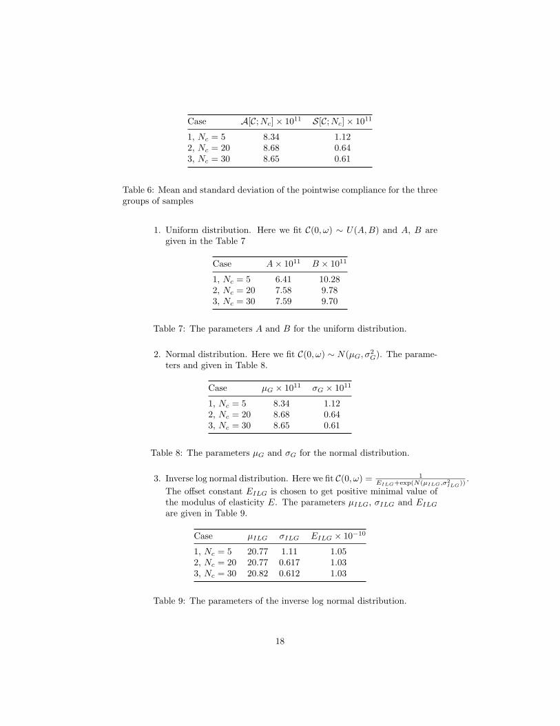
From the experimental data we get the mean and the standard deviationfor the three groups of measurements, shown in Table 6. Using these datawe get the parameters of the distributions:

BT73]

17

Case A[C;Nc]× 1011 S[C;Nc]× 1011

1, Nc = 5 8.34 1.122, Nc = 20 8.68 0.643, Nc = 30 8.65 0.61

Table 6: Mean and standard deviation of the pointwise compliance for the threegroups of samples

1. Uniform distribution. Here we fit C(0, ω) ∼ U(A,B) and A, B aregiven in the Table 7

Case A× 1011 B × 1011

1, Nc = 5 6.41 10.282, Nc = 20 7.58 9.783, Nc = 30 7.59 9.70

Table 7: The parameters A and B for the uniform distribution.

2. Normal distribution. Here we fit C(0, ω) ∼ N(µG, σ2G). The parame-

ters and given in Table 8.

Case µG × 1011 σG × 1011

1, Nc = 5 8.34 1.122, Nc = 20 8.68 0.643, Nc = 30 8.65 0.61

Table 8: The parameters µG and σG for the normal distribution.

3. Inverse log normal distribution. Here we fit C(0, ω) = 1EILG+exp(N(µILG,σ2

ILG)).

The offset constant EILG is chosen to get positive minimal value ofthe modulus of elasticity E. The parameters µILG, σILG and EILG

are given in Table 9.

Case µILG σILG EILG × 10−10

1, Nc = 5 20.77 1.11 1.052, Nc = 20 20.77 0.617 1.033, Nc = 30 20.82 0.612 1.03

Table 9: The parameters of the inverse log normal distribution.

18

4. Log-normal distribution. Here we fit C(0, ω) ∼ exp(N(µLG, σ2LG)).

The parameters µLG and σLGare given in Table 10.

Case µLG σLG

1, Nc = 5 -23.21 0.142, Nc = 20 -23.17 0.0783, Nc = 30 -23.17 0.074

Table 10: The parameters of the log normal distribution.

Fig. 8 shows the fitted cumulative distributions, together with the empir-ical one, for the three groups of measurements.

4 5 6 7 8 9 10 11 12x 10−11

0

0.1

0.2

0.3

0.4

0.5

0.6

0.7

0.8

0.9

1

C

F(C)

Marginal cumulative distribution for compliance, Nc = 5

EmpiricalGaussianUniformLognormalInverse Logn

(a)

3 4 5 6 7 8 9 10 11 12 13x 10−11

0

0.1

0.2

0.3

0.4

0.5

0.6

0.7

0.8

0.9

1

C

F(C)



(b)

3 4 5 6 7 8 9 10 11 12 13x 10−11

0

0.1

0.2

0.3

0.4

0.5

0.6

0.7

0.8

0.9

1

C

F(C)



(c)

Figure 8: The fitted and the empirical cumulative distributions for the threegroups of experiments: (a) Nc = 5, (b) Nc = 20, (c) Nc = 30.

b) Nonparametric distributions. Here we are using the kernel density function

19

based on two kernels, the Gaussian and the Epanetchnikov (for details see[BNT06]). The cumulative distribution based on the kernel density func-tion, together with the empirical one, for the three groups of measurementsare shown in Fig. 9.

4 5 6 7 8 9 10 11 12x 10−11

0

0.1

0.2

0.3

0.4

0.5

0.6

0.7

0.8

0.9

1

C

F(C)


EmpiricalGaussian KDEEpanetchnikov KDE

(a)

3 4 5 6 7 8 9 10 11 12 13x 10−11

0

0.1

0.2

0.3

0.4

0.5

0.6

0.7

0.8

0.9

1

CF(

C)



(b)

3 4 5 6 7 8 9 10 11 12 13x 10−11

0

0.1

0.2

0.3

0.4

0.5

0.6

0.7

0.8

0.9

1

C

F(C)



(c)

Figure 9: The cumulative distribution based on the kernel approach and theempirical distribution, for the three groups of the measurements: (a) Nc = 5,(b) Nc = 20, (c) Nc = 30.

Since the Gaussian and Epanetchnikov density functions are leading prac-tically to the same results, only the former will be considered below.

13.2 Ranking the models for the marginal distribution

In Section 13.1 we constructed various models of the marginal distribution.We have to rank them with respect to the goal of the analysis. We use thediscrepancy theory and the Kullback-Leibler measure (for details see [BNT06,KL51]) and use bootstrapping (see next section) to estimate the distribution ofsuch discrepancies. We rank then all considered parametric and nonparametric

20

Nc = 5 Nc = 20 Nc = 30 RankMarginal Median Mean Median Mean Median Mean (Median)

Uniform +Inf +Inf +Inf +Inf +Inf +Inf (5)Normal 1.38 +Inf 1.43 1.48 1.43 1.45 (3)LogNormal 1.97 1.96 2.31 2.29 2.32 2.31 (4)Inverse LN 1.04 1.26 1.19 1.20 1.26 1.27 (1)KDE 1.35 +Inf 1.28 1.36 1.32 1.35 (2)

Table 11: Ranking of various models by the mean and the median of the boot-strapped discrepancy.

marginal distributions according to the mean or median of the bootstrappeddiscrepancy distribution. Lower values characterize smaller discrepancy andhence higher quality of the model. The values are given in Table 11.

The uniform distribution leads to infinite discrepancy (for details see [BNT06]).We see that the inverse log-normal is the best, but the kernel density distribu-tion is close. Note that the kernel density distribution is not assuming anyparticular form of probability density function (pdf) and is robust.

13.3 Fitting the correlation length Lc

The covariance structure in (1) depends on two parameters, namely, α and thecorrelation length Lc. We will consider three cases: a) fully correlated randomfield (α = 0, Lc > 0), b) partially correlated random field (α = 2, Lc > 0) andc) perfectly uncorrelated field (α > 0, Lc = 0). These choices were selectedas the extreme cases although other intermediate cases could be considered aswell. To get feeling on the two extreme choices we show in Fig. 10 the raw datafor the compliance and elongation together with the relation between these databased on the models from the two extreme cases.

For α = 0 the compliance is constant over the entire length of the sampleand the relation between the compliance in the middle if the sample C(L/2)and the elongation δL is linear.

In the uncorrelated case the elongation is independent of the compliancevalue C(L/2). It is necessary to determine carefully this value from the rawdata for the three groups of experiments. (For detail see [BNT06]). We see thatthe fully correlated case gives very bad results, while the uncorrelated case isreasonable.

In the case α = 2 the correlation length Lc has to be determined. We ob-serve that formulas (1) and (2), allow to determine the cross-covariance betweenC(L/2) and the elongation δL, as well as the variance of δL, as a function ofLc. The same quantities (cross-covariance and variance) can also be determinedfrom the experimental data. The correlation length Lc is then determined byleast square so that the sample variance and cross-covariance are best fitted.The computed correlation length is given, for the three cases, in Table 12. The

21

6.5 7 7.5 8 8.5 9 9.5x 10−11

4

4.2

4.4

4.6

4.8

5

5.2

5.4

5.6x 10−5

C(L/2)

Calibration Experiment Data, Nc = 5

Calib

ratio

n El

onga

tion Measured Elongation

Elongation based on α=0Elongation based on Lc=0

(a)

6.5 7 7.5 8 8.5 9 9.5x 10−11

4

4.2

4.4

4.6

4.8

5

5.2

5.4

5.6

5.8

6x 10−5

C(L/2)


Calib

ratio

n El

onga

tion

Measured ElongationElongation based on α=0Elongation based on Lc=0

(b)

6.5 7 7.5 8 8.5 9 9.5x 10−11

4

4.2

4.4

4.6

4.8

5

5.2

5.4

5.6

5.8

6x 10−5

C(L/2)


Calib

ratio

n El

onga

tion

Measured ElongationElongation based on α=0Elongation based on Lc=0

(c)

Figure 10: Elongation and point compliance data from the calibration exper-iment as well as the two extreme models, for the three groups of calibrationexperiments: (a) Nc = 5, (b) Nc = 20, (c) Nc = 30

computed correlation length Lc was practically independent of the marginaldistribution model.

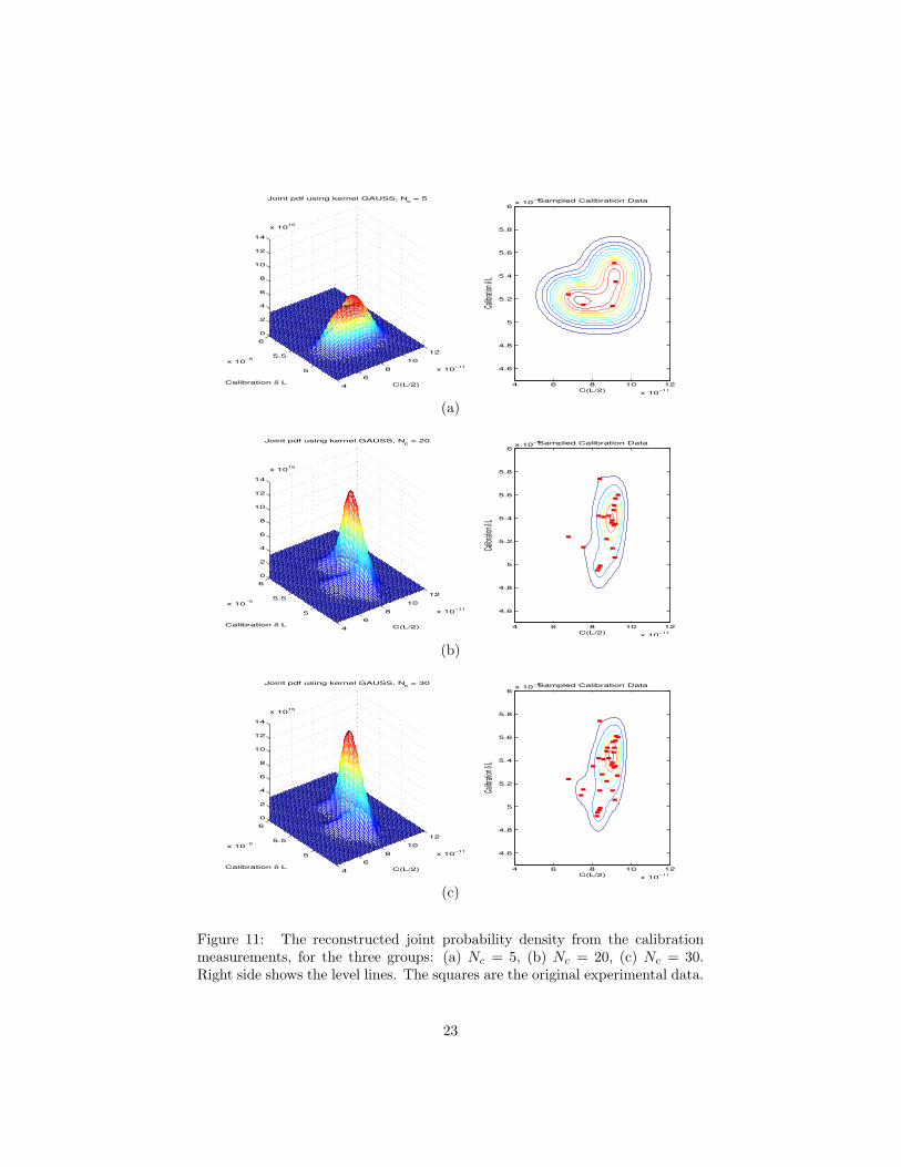
13.4 Variability in the fitted data

The variability of the parameters of the compliance models is very essential toestablish the confidence in the model, especially in presence of a small set ofexperimental data. It is done by the boot-strapping approach [Efr82, ET93] asfollows. The joint probability density function of C(L/2) and δL is reconstructedby the Gaussian kernel density approach. The reconstruction is shown in Fig.11.

We draw samples of size Nc from the reconstructed pdf, and fit the param-eters of the compliance model, as described in the previous sections, for eachbootstrapped sample. We repeat the procedure B = 1000 times and get a distri-bution for the fitted parameters. In Fig. 12 we show the bootstrapped samples

22

46

810

12

x 10−115

5.5

6

x 10−5

0

2

4

6

8

10

12

14

x 1015

C(L/2)

Joint pdf using kernel GAUSS, Nc = 5

Calibration δ LC(L/2)

Calibra

tion δ L

Sampled Calibration Data

4 6 8 10 12x 10−11

4.6

4.8

5

5.2

5.4

5.6

5.8

6x 10−5

(a)

46

810

12

x 10−115

5.5

6

x 10−5

0

2

4

6

8

10

12

14

x 1015

C(L/2)



Calibra

tion δ L


4 6 8 10 12x 10−11

4.6

4.8

5

5.2

5.4

5.6

5.8

6x 10−5

(b)

46

810

12

x 10−115

5.5

6

x 10−5

0

2

4

6

8

10

12

14

x 1015

C(L/2)



Calibra

tion δ L


4 6 8 10 12x 10−11

4.6

4.8

5

5.2

5.4

5.6

5.8

6x 10−5

(c)

Figure 11: The reconstructed joint probability density from the calibrationmeasurements, for the three groups: (a) Nc = 5, (b) Nc = 20, (c) Nc = 30.Right side shows the level lines. The squares are the original experimental data.

23

Case Lc (m)

1, Nc = 5 0.0092, Nc = 20 0.0303, Nc = 30 0.035

Table 12: The correlation length Lc determined from three sets of experimentaldata.

and the original experimental data.Similarly it is possible to reconstruct the marginal distribution for C(L/2)

separately (or use the data from the joint probability). Then the bootstrappedcumulative distribution of the pointwise compliance can be computed (see Fig.12 right). We see how the width of the distribution function decreases withincreasing number of experiments. This width is related to the confidence inthe cumulative distribution function.

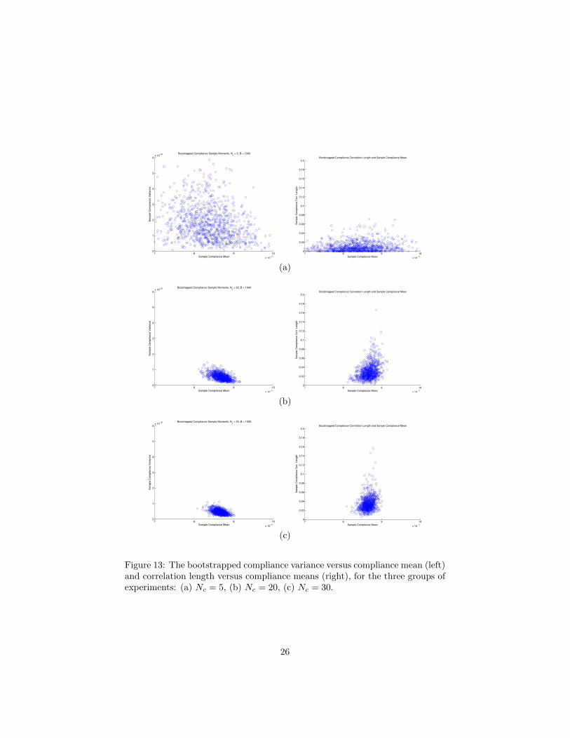
In Fig. 13 we show the bootstrapped sample compliance variance versus thecompliance mean (left) and the sample compliance correlation length Lc versusthe compliance mean. These figures show the confidence of the mean, varianceand correlation length.

13.5 On the model and the calibration data

We considered a few models based on different marginal probabilities and co-variance form (1). We concluded that two marginal distributions, the inverselog normal and the kernel density function lead to the best results. It was seenthat the partially correlation model gives very reasonable results while the fullycorrelated model is inappropriate. The perfectly uncorrelated model gives prac-tically acceptable results. It was clear that various models should be consideredand ranked. The small number of experimental data significantly influences theapproach. The model we consider is a stochastic model, which already char-acterizes the aleatory uncertainty. Nevertheless, we still have uncertainties ofepistemic type stemming from the small number of experimental data. Thestatistical analysis addressed in this section relates to the quantification of theuncertainties as discussed in general in section 5 and particularly in Section 10.After finishing the calibration, we proceed to the validation phase.

14 The Validation process

The goal of the validation is to assess reliability of the calibrated model. Thereis a much smaller number of validation experiments than for calibration. Theprocess which is used in this paper has three parts:

a) Using the calibrated model, the probability field of the validation elonga-tion is constructed, typically by the Monte Carlo method;

24

4 5 6 7 8 9 10 11 12x 10−11

4.6

4.8

5

5.2

5.4

5.6

5.8

6x 10−5

C(L/2)

Calib

ratio

n El

onga

tion

Boostrapped Compliance and Elongation Samples, Nc = 5, B = 100

Bootstrapped Compliance and Elongation SamplesOriginal Compliance and Elongation Samples

4 5 6 7 8 9 10 11 12x 10−11

0

0.1

0.2

0.3

0.4

0.5

0.6

0.7

0.8

0.9

1

C

CDF(

C)

Boostrapped Compliance CDF, Nc = 5, B = 100

(a)

4 5 6 7 8 9 10 11 12x 10−11

4.6

4.8

5

5.2

5.4

5.6

5.8

6x 10−5

C(L/2)

Calib

ratio

n El

onga

tion



4 5 6 7 8 9 10 11 12x 10−11

0

0.1

0.2

0.3

0.4

0.5

0.6

0.7

0.8

0.9

1

C

CDF(

C)


(b)

4 5 6 7 8 9 10 11 12x 10−11

4.6

4.8

5

5.2

5.4

5.6

5.8

6x 10−5

C(L/2)

Calib

ratio

n El

onga

tion



4 5 6 7 8 9 10 11 12x 10−11

0

0.1

0.2

0.3

0.4

0.5

0.6

0.7

0.8

0.9

1

C

CDF(

C)


(c)

Figure 12: On the left: 100 bootstrapped samples from the reconstructed jointpdf of C(L/2) and δL, for the three groups of experiments: (a) Nc = 5, (b) Nc =10, (c) Nc = 30. On the right: bootstrapped empirical cumulative distributionof the compliance.

25

7 8 9 10x 10−11

0

1

2

3

4

5

6x 10−22 Boostrapped Compliance Sample Moments, Nc = 5, B = 1000

Sample Compliance Mean

Sam

ple

Com

plia

nce

Varia

nce

7 8 9 10x 10−11

0

0.02

0.04

0.06

0.08

0.1

0.12

0.14

0.16

0.18

0.2Bootstrapped Compliance Correlation Length and Sample Compliance Mean


Sam

ple

Com

plia

nce

Corr.

Len

gth

(a)

7 8 9 10x 10−11

0

1

2

3

4

5



Sam

ple

Com

plia

nce

Varia

nce

7 8 9 10x 10−11

0

0.02

0.04

0.06

0.08

0.1

0.12

0.14

0.16

0.18



Sam

ple

Com

plia

nce

Corr.

Len

gth

(b)

7 8 9 10x 10−11

0

1

2

3

4

5



Sam

ple

Com

plia

nce

Varia

nce

7 8 9 10x 10−11

0

0.02

0.04

0.06

0.08

0.1

0.12

0.14

0.16

0.18



Sam

ple

Com

plia

nce

Corr.

Len

gth

(c)

Figure 13: The bootstrapped compliance variance versus compliance mean (left)and correlation length versus compliance means (right), for the three groups ofexperiments: (a) Nc = 5, (b) Nc = 20, (c) Nc = 30.

26

b) Using the available validation measurements a Bayesian update of thecompliance model parameters is computed. A noninformative prior ( see[Tan96, Jef98] ) is used. The updating is in some cases computationallyintensive. The updated model is assumed to be much more accurate thenthe calibrated one.

c) Using both the calibrated and updated model, the probability distribu-tion of the quantity of interest (in the prediction problem) is constructed.A notion of the distance between these two probability distributions isdefined; this distance is used as the metric. The reason for it is that themetric has to be closely related to the quantity of interest, i.e. the goal ofthe analysis. The distance is also used for the definition of the rejectioncriterion. Based on it and the given tolerance the calibrated model couldbe rejected

14.1 The distance between two cumulative distributionsand the rejection criterion

Definition 1 (Horizontal distance between CDFs) Let F,G : R → [0, 1]be two cumulative distributions and Iε(G) the ε−level

Iε(G) ≡ x ∈ R | ε

2≤ G(x) ≤ 1− ε

2.

We define the distance between F and G as

dε(F,G) := maxx∈Iε(G)

|F−1 G(x)− x| (5)

The distance is well suited for the quantity of interest which has to be pre-dicted, i.e. the probability that the displacement in the point Pm is not exceed-ing 3mm.

Fig. 14 gives graphical interpretation of the distance.

I (G )ε

εI (G)

ε/2

1−ε/2

F(x)

G(x)

x in

1

h(x)

x

d = max h(x)

Figure 14: The graphical interpretation of the distance, which is related to themetric used in the validation.

The idea of the distance is the following. Assume that Y is the true value ofthe quantity of interest and Y cal resp Y up are the quantities predicted by the

27

calibrated, respectively updated, model. Then we assume that

dε(FY , FY cal) ≈ dε(FY up , FY cal). (6)

The value of the parameter ε is more or less arbitrary. We selected ε = 0.005.The reason is to avoid the reliance on the tail which is unstable and practicallynot significant if it is sufficiently small as in our case. Then the neighborhoodof size +/- ε is used as the probability box which characterizes the reliability ofthe model. This leads directly to the definition of the metric and the criterionbased on a given tolerance tol:

Definition 2 (Rejection criterion) Given a tolerance level tol we reject themodel Y cal if

dε(FY up , FY cal) ≥ tol × 3mm (7)

The value of the tolerance could be different and has to be related to the deci-sion based on the computed data. Selecting a larger tolerance, the cruder andsimpler model will not be rejected but the reliability of the prediction will besmaller. This has to be taken into consideration when the decision (for whichthe computation is the basis) is made. If the tolerance is small, then possiblyall models will be rejected when only small number of data is available. Themodels not rejected could be much more complex and computationally moreexpensive. In what follows we use tol = 0.10. Let us mention that rejectiondepends not only on the tolerance but also on the value of the parameter ε andthe selection of both depends on the purpose of the computation.

14.2 The Bayesian updating of the parameters

For every model we compute the updated parameters using the noninformativeprior. Here we will report only the mean and standard deviation of updatedmarginal distribution, for the three models:

(a) Full correlation, α = 0, Lc > 0. In Table 13 we give the ratio of the meansand standard deviations (std) between the updated and the calibratedmodels.

Uniform Normal Inverse LNCase µup

U

µcalU

σupU

σcalU

µupG

µcalG

σupG

σcalG

E[C(0)]up

E[C(0)]cal

std[C(0)]up

std[C(0)]cal

1, Nv = 2 1.02 0.055 1.02 0.1 1.01 0.12, Nv = 4 0.98 0.14 0.98 0.2 0.97 0.23, Nv = 10 0.99 0.26 0.99 0.3 0.98 0.3

Table 13: The ratio of the calibrated and updated means and std for uniform,normal and inverse log normal marginal distribution and full correlation.

28

(b) Partial correlation, α = 2, and calibrated value of Lc. In this case, we donot update the covariance length Lc because Lv Lc and the influenceof specific value of Lc is very small. In Table 14 we show the ratios forthe partial correlation model, for uniform, normal and inverse log normalmarginal distributions

Uniform Normal Inverse LNCase µup

U

µcalU

σupU

σcalU

µupG

µcalG

σupG

σcalG

E[C(0)]up

E[C(0)]cal

std[C(0)]up

std[C(0)]cal

1, Nv = 2 1.01 0.57 1.01 0.56 1.02 0.572, Nv = 4 0.98 0.81 0.98 0.80 0.98 0.803, Nv = 10 0.99 0.98 0.99 1.00 0.98 1.00

Table 14: The ratio of the calibrated and updated means and std for the uniform,normal and inverse log normal marginal distributions for the partial correlationmodel.

(c) Perfect non-correlation, Lc = 0. This case has to be handled differentlybecause the problem become deterministic with the material described bythe effective modulus Eeff only. The predicted elongation has std = 0and depends only on the mean value µ independently of the marginaldistribution. Hence only the mean can be updated. Yet this updatinghas a drawback because its variation cannot be updated and hence theassumption that the updated model is accurate does not hold. Thereforeas a more accurate model we use the normal distribution with the updatedmean and the standard deviation computed from the measured data.

14.3 Distance computation and model rejection

Once we have updated the models we can compute the cumulative distributionof the predicted quantity of interest by the calibrated and the updated models.Then we compute the distance between both distributions. Table 15 shows theratio of the distance and the critical displacement 3mm for the three groups ofthe validation experiments. In boldface are the rejected models for a tolerancetol = 0.10. We see that for the tolerance tol = 0.10 the fully correlated modelhas to be rejected for all marginal distributions although its reliability slightlygrows with the increase of the number of experiments. Of course this model isthe simplest one. The partial correlation model leads to the best results for allmarginal distributions. The completely uncorrelated one still leads to a reason-able accuracy and it is computationally simpler than the partially correlatedmodel. Hence we do reject the completely correlated model and keep the par-tially correlated and uncorrelated ones. Note that the ratios in Table 15 arenot in all cases decreasing when increasing the number of experiments. This iscaused by the influence of the small number of experiments.

29

Case 1 Case 2 Case 3(Nc, Nv) = (5, 2) (20, 4) (30, 10)

(a) Fully correlated model α = 0

Uniform 0.25 0.14 0.12Normal 0.25 0.13 0.11Inverse LN 0.25 0.17 0.12

(b) Partially correlated model α = 2


(c) Perfectly uncorrelated model Lc = 0

Effective model 0.07 0.08 0.09

Table 15: The ratio of the horizontal distances and the critical prediction dis-placement.

To further illustrate the results we show, on the left side of Fig. 15 the cumu-lative distribution of the elongation Lv, empirical, predicted by the calibratedmodel and by the updated one, for the uniform marginal and fully correlatedmodel. On the right side we show the cumulative distribution of the quantity ofinterest (prediction) and the bounds based on the computed distance. Note thaton the left the cumulative distribution of the elongation Lv has been computedanalytically, while on the right the cumulative distribution has been computedby the Monte Carlo Method (although it could also have been computed analyt-ically as well). In Fig. 16 we show analogous results for the partially correlatedmodel with normal marginal distribution.

15 The accreditation

The accreditation process is analogous to the validation one. We have to takehere into account that only a very small number of experimental data is avail-able. Using the calibrated model we compute the displacement of the midpointQ of bar 1 in the accreditation frame, and by the Bayesian approach we updatethe mean and the std of the compliance model using the available accreditationmeasured data. In the case when only one experiment is available, only the meanis updated and. Then we compute the cumulative distribution of the quantity

30

1.4 1.6 1.8 2 2.2 2.4 2.6

x 10−4

0

0.1

0.2

0.3

0.4

0.5

0.6

0.7

0.8

0.9

1

δ Lv

F(δ

Lv)

Validation, CASE 1, UNIFORM, α = 0

ModelUpdated parametricEmpiricalExperiment Data

−3.5 −3 −2.5

x 10−3

0

0.1

0.2

0.3

0.4

0.5

0.6

0.7

0.8

0.9

1

w(Pm

), Horizontal distance = 0.75x 10−3

F(w

(Pm

))

Model prediction vs. updated: UNIFORM, α = 0, Updated using Validation DATA, CASE 1

Modellower boundupper boundUpdated Model

Case 1: Nc = 5, Nv = 2

1.8 1.9 2 2.1 2.2 2.3 2.4

x 10−4

0

0.1

0.2

0.3

0.4

0.5

0.6

0.7

0.8

0.9

1

δ Lv

F(δ

Lv)



−3.5 −3 −2.5

x 10−3

0

0.1

0.2

0.3

0.4

0.5

0.6

0.7

0.8

0.9

1

w(Pm


F(w

(Pm

))



Case 2: Nc = 20, Nv = 4

1.8 1.9 2 2.1 2.2 2.3 2.4

x 10−4

0

0.1

0.2

0.3

0.4

0.5

0.6

0.7

0.8

0.9

1

δ Lv

F(δ

Lv)



−3.5 −3 −2.5

x 10−3

0

0.1

0.2

0.3

0.4

0.5

0.6

0.7

0.8

0.9

1

w(Pm


F(w

(Pm

))



Case 3: Nc = 30, Nv = 10

Figure 15: The uniform marginal distribution and full correlation. On theleft is the cumulative distribution of the elongation Lv, empirical, predicted bythe calibrated model and by the updated one. On the right is the cumulativedistribution of the quantity of interest with the bounds based on the distance.The bounds are creating the probability box.

31

1.85 1.9 1.95 2 2.05 2.1 2.15

x 10−4

0

0.1

0.2

0.3

0.4

0.5

0.6

0.7

0.8

0.9

1

δ Lv

F(δ

Lv)

Validation, CASE 1, NORMAL, α = 2

Sampled ModelModel parametricUpdated parametricEmpiricalExperiment Data

−3.5 −3 −2.5

x 10−3

0

0.1

0.2

0.3

0.4

0.5

0.6

0.7

0.8

0.9

1

w(Pm


F(w

(Pm

))

Model prediction vs. updated: NORMAL, α = 2, Updated using Validation DATA, CASE 1


Case 1: Nc = 5, Nv = 2

1.95 2 2.05 2.1 2.15 2.2 2.25

x 10−4

0

0.1

0.2

0.3

0.4

0.5

0.6

0.7

0.8

0.9

1

δ Lv

F(δ

Lv)



−3.5 −3 −2.5

x 10−3

0

0.1

0.2

0.3

0.4

0.5

0.6

0.7

0.8

0.9

1

w(Pm


F(w

(Pm

))



Case 2: Nc = 20, Nv = 4

1.9 1.95 2 2.05 2.1 2.15 2.2

x 10−4

0

0.1

0.2

0.3

0.4

0.5

0.6

0.7

0.8

0.9

1

δ Lv

F(δ

Lv)



−3.5 −3 −2.5

x 10−3

0

0.1

0.2

0.3

0.4

0.5

0.6

0.7

0.8

0.9

1

w(Pm


F(w

(Pm

))



Case 3: Nc = 30, Nv = 10

Figure 16: The partially correlated model with normal marginal distribution.On the left is the cumulative distribution of the elongation Lv, empirical, pre-dicted by the calibrated model and by the updated one. On the right is theprobability box for the quantity of interest, based on the computed distance.

32

of interest in the prediction problem using the calibrated and updated modeland compute the distance of these two distributions. In Table 16 we give theratio of the distance and the critical value. Because the fully correlated modelwas rejected on the validation level we do not address it in the accreditationphase. From the table we see that with the tolerance tol = 0.1 we do not reject

Case 1 Case 2 Case 3(Nc, Na) = (5, 1) (20, 1) (30, 2)

(a) Partially correlated model α = 2


(b) Perfectly uncorrelated model Lc = 0

Effective model 0.072 0.072 0.1

Table 16: The ratio of the distance and the critical value, in the accreditationprocedure, for the partially correlated models and the perfectly uncorrelatedmodel.

the models, with the exception of the perfectly uncorrelated model in the case3.

16 The prediction

As we have said above the prediction is based on the calibrated model taking intoaccount also the variability in the fitted data, estimated by bootstrapping, es-pecially in the case of a small number of calibration experiments. The distancescomputed in the validation and accreditation processes are used for determiningbounds in the predicted failure. The goal is to approximate P (w(Pm) > 3mm)where w(Pm) is the displacement in the midpoint Pm of the bar 4 in the frame.To properly account for the variability in the prediction due to the small amountof calibration information, we consider the parameters defining the compliancemodel (2) (hereafter denoted by Θ) as random variables and sample them bybootstrapping, using the procedure described in Section 13.4. If (Ω, F , P ) isthe probability space for Θ and (Ω,G, Q) is the probability space for the modelprediction displacement for a given Θ, then

P (|w(Pm,Θ)| ≥ 3(mm)) =∫

Ω

∫Ω

1|w(Pm,Θ(ω),ω)|≥3(mm)dQ(ω)dP (ω). (8)

33

Given two natural numbers B and M we hierarchically sample first B times themodel parameters Θ by bootstrapping, then, for each sampled Θ, we samplew(Pm,Θ) M times to generate B ×M corresponding bootstrap samples. Thisis computationally intensive and various simplification described in [BNT06]have been made. This procedure is important when only a small number ofcalibration experiments is available. We note that also for a large numberof experiments the bootstrapping results will not coincide with the predictionbased on the calibrated model. This is because the calibrated model is onlyapproximate. In Table 17 we are giving the failure probability evaluated by thebootstrapping for various marginal probability distributions.

Case 1 Case 2 Case 3(Nc, Nv, Na) = (5, 2, 1) (20, 4, 1) (30, 10, 2)

Uniform 2.0× 10−2 4.7× 10−5 5.6× 10−8

Normal 2.1× 10−2 5.8× 10−5 8.6× 10−8

Inverse LN 1.4× 10−2 4.6× 10−5 5.6× 10−8

Table 17: Failure probabilities for the prediction displacement P (|w(Pm)| ≥3mm), evaluated with the bootstrapping procedure for the partially correlatedmodels.

We augment the results by the information we have obtained during thevalidation and accreditation phases to get bounds. For this, instead of providingas failure probability the quantity P (|w(Pm)| > 3mm) we use P (|w(Pm)| >3(1 ± dε)mm), where dε is the maximum of the distances measured in thevalidation and the accreditation phases. In Table 18 we show upper boundson the failure probability, evaluated by combining the bootstrapping and thedistances in the validation and accreditation procedure.

Case 1 Case 2 Case 3(Nc, Nv, Na) = (5, 2, 1) (20, 4, 1) (30, 10, 2)

Uniform 0.18 1.8× 10−2 3.0× 10−3

Normal 0.19 2.1× 10−2 2.1× 10−3

Inverse LN 0.19 1.7× 10−2 1.4× 10−3

Table 18: The probability of failure bounds obtained by combining the boot-strapping procedure with the distances measured in the validation and accredita-tion experiments, for various marginal probabilities and the partially correlatedmodel.

In Fig. 17 we show the cumulative distribution of the prediction quantity

34

computed by the calibrated model and by the bootstrapped one (which accountsalso for the variability of the compliance model parameters) for the normalmarginal distribution and partial correlation. In addition we show the boundsbased on the distances in the validation and accreditation. In Fig. 18 we showanalogous results for the perfectly uncorrelated model.

−3.2 −3 −2.8 −2.6 −2.4 −2.2 −2x 10−3

0

0.1

0.2

0.3

0.4

0.5

0.6

0.7

0.8

0.9

1

w(Pm)

F(w(

P m))

Bootstrapped prediction values, Data case 1, using NORMAL, α = 2,

PredictionBoundBoundBoostrapped Prediction

Case 1: Nc = 5, Nv = 2, Na = 1

−3 −2.9 −2.8 −2.7 −2.6 −2.5 −2.4x 10−3

0

0.1

0.2

0.3

0.4

0.5

0.6

0.7

0.8

0.9

1

w(Pm)

F(w(

P m))



Case 2: Nc = 20, Nv = 4, Na = 1

−3 −2.95 −2.9 −2.85 −2.8 −2.75 −2.7 −2.65 −2.6 −2.55x 10−3

0

0.1

0.2

0.3

0.4

0.5

0.6

0.7

0.8

0.9

1

w(Pm)

F(w(

P m))



Case 3: Nc = 30, Nv = 10, Na = 2

Figure 17: The cumulative distribution of the predicted quantity of interestobtained by the calibrated model (blue), the bootstrapped model (green) andthe bounds. Partially correlated model with Normal marginal distribution.

From Figures 17 and 18 we see that for the case of the smallest numberof experimental data the bootstrapping is essential. For the higher number of

35

−3.6 −3.4 −3.2 −3 −2.8 −2.6 −2.4 −2.2 −2 −1.8x 10−3

0

0.1

0.2

0.3

0.4

0.5

0.6

0.7

0.8

0.9

1

w(Pm)

F(w(

P m))

Bootstrapped prediction values, Data case 1, using NORMAL, Lc = 0,


Case 1: Nc = 5, Nv = 2, Na = 1

−3.4 −3.2 −3 −2.8 −2.6 −2.4 −2.2x 10−3

0

0.1

0.2

0.3

0.4

0.5

0.6

0.7

0.8

0.9

1

w(Pm)

F(w(

P m))



Case 2: Nc = 20, Nv = 4, Na = 1

−3.4 −3.2 −3 −2.8 −2.6 −2.4 −2.2x 10−3

0

0.1

0.2

0.3

0.4

0.5

0.6

0.7

0.8

0.9

1

w(Pm)

F(w(

P m))



Case 3: Nc = 30, Nv = 10, Na = 2

Figure 18: The cumulative distribution of the predicted quantity of interest bythe calibrated (blue) and the bootstrapped model ( green ) for the perfectlyuncorrelated model.

36

experiments the influence of the “modeling error”, quantified by distances mea-sured in the validation and accreditation, is larger than the variability relatedto the number of experiments, estimated by bootstrapping.

Comparing Figs. 17 and 18 we see that the use of the bounds is essentialfor the confidence in the perfectly uncorrelated model which is less reliable thanthe partially correlated model.

17 Conclusions

We have shown the general process of the prediction based on the calibration,validation and accreditation. We have seen the role of the number of experi-mental data. If the number is small then the accuracy of the prediction can bevery unreliable and the decision has to take it properly into consideration.

The validation analysis for the academic frame problem was based on theBayesian probability. This approach may be costly in general, yet there areways to perform the Bayesian update approximately, thus reducing the com-putational cost. Other techniques such as sensitivity analysis or worst-casescenario approach could be used as well.

In our problem we neglected the errors in the experiments. These of coursehave to be addressed in any analysis too. Many approaches to the problemof validation under uncertainties exist. In our academic problem the exactsolution i.e. the probability of the failure is not available. It seems to be veryimportant to develop various approaches and test them on problems where theexact solution is known (the manufactured problems). In the general case, asfor instance the airplane design, the situation is much more complex and manytheoretical and implementational issues are open. The problem of the adaptivemodeling which leads to the best results with minimal cost is also essential.

Acknowledgments

We would like to thank Dr. Laurent Chambon (EADS-CCR) and Dr. StephaneGuinard (EADS-CCR) for valuable comments.

References

[AIA98] Guide for verification and validation of computational fluid dynamicssimulation. Technical Report AIAA G-077-1998, American Instituteof Aeronautics and Astronautics, 1998.

[Bab61] I. Babuska. On randomized solutions of Laplace’s equation. CasopisPest. Math., 86:269–276, 1961.

[BJLS93] I. Babuska, K. Jerina, Y. Li, and P. Smith. Quantitative assesmentof the accuracy of constitutive laws for plasticity with an exposureon cyclic deformation. Material Parameter Estimation for Modern

37

Constitutive Equations, ASME, MD-Vol 43/ AMD- Vol 168:116–169,1993.

[BLT03] I. Babuska, K-M. Liu, and R. Tempone. Solving stochastic partialdifferential equations based on the experimental data. Math. ModelsMethods Appl. Sci., 13(3):415–444, 2003. Dedicated to Jim Douglas,Jr. on the occasion of his 75th birthday.

[BNT05] I. Babuska, F. Nobile, and R. Tempone. Worst-case scenario analysisfor elliptic problems with uncertainty. Numer. Math., 101:185–219,2005.

[BNT06] I. Babuska, F. Nobile, and R. Tempone. Model validation challangeproblem: Static frame prediction. sandia validation workshop. SAN-DIA Workshop, May 27-29,2006, 2006.

[BO04] I. Babuska and J-T. Oden. Verification and Validation in Comptua-tional Engineering and Science. Part I: Basic concepts. Comp. Meth.Appl..Mech. Engrg., 193:4057–4061, 2004.

[BO05] I. Babuska and J-T. Oden. The reliability of computer predictions;can they be trusted. Int. J. Num. Anal. Mode., 3, 2005.

[BS01] I. Babuska and T. Strouboulis. The Finite Element Method and itsReliability. Oxford University Press, 2001.

[BT73] G. E. P. Box and G. C. Tiao. Bayesian inference in statistical analysis.Addison-Wesley Publishing Co., Reading, Mass.-London-Don Mills,Ont., 1973. Addison-Wesley Series in Behavioral Science: Quantita-tive Methods.

[BTZ04] I. Babuska, R. Tempone, and G.E. Zouraris. Galerkin finite ele-ment approximations of stochastic elliptic partial differential equa-tions. SIAM J. Numer. Anal., 42(2):800–825 (electronic), 2004.

[BTZ05] I. Babuska, R. Tempone, and G.E. Zouraris. Solving elliptic bound-ary value problems with uncertain coefficients by the finite elementmethod: the stochastic formulation. Comput. Methods Appl. Mech.Engrg., 194(12-16):1251–1294, 2005.

[CF99] A.C. Cullen and H.C. Frey. Probabilistic Techniques Exposure Assess-ment. Plenum Press, 1999.

[Efr82] B. Efron. The jackknife, the bootstrap and other resampling plans, vol-ume 38 of CBMS-NSF Regional Conference Series in Applied Math-ematics. Society for Industrial and Applied Mathematics (SIAM),Philadelphia, Pa., 1982.

[ET93] B. Efron and R. J. Tibshirani. An introduction to the bootstrap, vol-ume 57 of Monographs on Statistics and Applied Probability. Chapmanand Hall, New York, 1993.

38

[HCB04] J. Hlavacek, I. Chleboun, and I. Babuska. Uncertain input data prob-lems and the worst scenario method. Elsevier, Amsterdam, 2004.

[Jay03] E. T. Jaynes. Probability theory. Cambridge University Press, Cam-bridge, 2003. The logic of science, Edited and with a foreword by G.Larry Bretthorst.

[Jef98] Harold Jeffreys. Theory of probability. Oxford Classic Texts in thePhysical Sciences. The Clarendon Press Oxford University Press, NewYork, 1998. Reprint of the 1983 edition.

[KL51] S. Kullback and R. A. Leibler. On information and sufficiency. Ann.Math. Statistics, 22:79–86, 1951.

[KOG98] G.B. Kleindorfer, L. O’Neil, and R. Ganeshan. Validation in simu-lation; various positions in the philosophy of science. ManagementScience, 44:1087–1099, 1998.

[Lee04] P. M. Lee. Bayesian statistics. Arnold, London, third edition, 2004.An introduction.

[McD04] D. McDonald. Elements of applied probability for engineering, math-ematics and systems science. World Scientific Publishing Co. Inc.,River Edge, NJ, 2004.

[NF67] T.H. Naylor and J.M. Finger. Verification of computer simulationmodel. Management Science, 14:B92– B103, 1967.

[OT02] W.L. Oberkampf and T.G. Trucano. Verification and validationin computational fluid dynamics. Progress in Aerospace Sciences,38:209–272, 2002.

[Pos04] D.E. Post. The coming crisis in computational sciences. Technical Re-port Rep.LA-UR-03-88-2004, Los Alamos National Laboratory, 2004.

[Roa98] P.J. Roache. Verification and Validation in Computational Scienceand Engineering. Hermosa, Albuquerque, New Mexico, 1998.

[Tan96] M. A. Tanner. Tools for statistical inference. Springer Series in Statis-tics. Springer-Verlag, New York, third edition, 1996. Methods for theexploration of posterior distributions and likelihood functions.

39

reliability of computational science

Documents