Contents lists available at ScienceDirect

Signal Processing

journal homepage: www.elsevier.com/locate/sigpro

Review

Relevance of polynomial matrix decompositions to broadband blind signalseparation

Soydan Redifa,⁎, Stephan Weissb,1, John G. McWhirterc

a Department of Electrical & Electronic Engineering, European University of Lefke, Lefke, North Cyprusb Department of Electronic & Electrical Engineering, University of Strathclyde, Glasgow G11XW, Scotlandc Cardiff University, Cardiff CF24 3AA, Wales, UK

A R T I C L E I N F O

Keywords:Paraunitary matrixParahermitian matrixPolynomial matrix eigenvalue decompositionBroadband blind signal separationBroadband adaptive beamformingRadarSonar

A B S T R A C T

The polynomial matrix EVD (PEVD) is an extension of the conventional eigenvalue decomposition (EVD) topolynomial matrices. The purpose of this article is to provide a review of the theoretical foundations of thePEVD and to highlight practical applications in the area of broadband blind source separation (BSS). Based onbasic definitions of polynomial matrix terminology such as parahermitian and paraunitary matrices, strongdecorrelation and spectral majorisation, the PEVD and its theoretical foundations will be briefly outlined. Thepaper then focuses on the applicability of the PEVD and broadband subspace techniques — enabled by thediagonalisation and spectral majorisation capabilities of PEVD algorithms — to define broadband BSS solutionsthat generalise well-known narrowband techniques based on the EVD. This is achieved through the analysis ofnew results from three exemplar broadband BSS applications — underwater acoustics, radar cluttersuppression, and domain-weighted broadband beamforming — and their comparison with classical broadbandmethods.

1. Introduction

Over the last decade, algorithms that extend the eigenvaluedecomposition (EVD) to the realm of polynomial matrices have had agrowing impact on signal processing theory and practice, mainlybecause they can be used to solve generalisations of narrowbandproblems typically addressed by the EVD, including subspace decom-position. The extension of EVD to parahermitian (PH) polynomialmatrices, referred to as polynomial matrix EVD (PEVD), gives animmediate broadband generalisation of the concepts of signal andnoise subspaces, and hence subspace decompositions. Just as principalcomponent analysis (PCA) based on the EVD is fundamental to mostnarrowband BSS formulations, the PEVD can be a powerful tool forbroadband or convolutive blind source separation (BSS).

The classical approach to narrowband BSS begins by exploitingsecond-order statistics to generate uncorrelated sequences from nar-rowband, instantaneously mixed signals by performing principalcomponent analysis (PCA) [1,2]. PCA is usually obtained throughmatrix factorisation by means of a unitary matrix decomposition, suchas the singular value (SVD) or eigenvalue decomposition (EVD) [3,4].To complete the BSS process, a “hidden” rotation matrix is determinedvia on higher-order statistics (HOS), which permutes entries to achieve

spectral coherence across frequency bins. With little or no priorknowledge and minimal assumptions, a BSS method can often be usedto extract a wanted signal from among interference signals. However,the wanted signal is in no way accentuated by these underlyingassumptions.

Incorporation of a priori knowledge of the signals into the BSSproblem can be formulated in the framework of signal decompositionsand matrix factorisations, and address statistical dependence, periodi-city, spectral shape, time coherence or smoothness [5–8]. The goaloften is to estimate a reduced coordinate space, which provides a moreaccurate physical representation of the sources or mixing parameters.

The above signal decompositions are based on an instantaneousmixing model, where the propagation of signals from sources to thearray is modelled as a scalar mixing matrix. However, in manyimportant applications such as broadband array processing, convolu-tive mixing — or a matrix of finite impulse response (FIR) filters —must be used instead. The transfer function of such a matrix of FIRfilters forms a polynomial matrix, which can accurately model effectssuch as multipath propagation, or the lag-dependent correlationbetween different broadband sensor signals. SVD- or EVD-baseddecompositions generally can only decorrelate instantaneously, i.e.,only for zero lag. Following convolutive mixing, strong decorrelation

http://dx.doi.org/10.1016/j.sigpro.2016.11.019Received 26 May 2016; Received in revised form 7 October 2016; Accepted 24 November 2016

⁎ Corresponding author.

1 EURASIP Member.E-mail addresses: sredif@eul.edu.tr (S. Redif), stephan.weiss@strath.ac.uk (S. Weiss), mcwhirterjg@cardiff.ac.uk (J.G. McWhirter).

Signal Processing 134 (2017) 76–86

Available online 25 November 20160165-1684/ © 2016 Elsevier B.V. All rights reserved.

MARK

[9] eliminates correlation for all lag values, and can be achieved using awell-designed matrix of FIR filters.

In the past, broadband BSS has been addressed by performingnarrowband BSS at each frequency bin simultaneously, throughapplication of the discrete Fourier transform (DFT) — commonlyreferred to as independent frequency bin (IFB) processing. However,coherence restoration is required after BSS via permutation matricesapplied in every bin [10,11]. An alternative is to adopt coherent signalsubspace-related methods, which generally require some prior knowl-edge of signals, such as direction and fractional bandwidth, tocoherently combine covariance matrices across different bins in orderto create an approximately narrowband problem [12–14].

The formulation and decomposition of polynomial matrices pre-sents an alternative to these classical broadband BSS approaches.Polynomial matrices have been used for many years, e.g., in the area ofcontrol [15] or broadband subspace decomposition and adaptivesensor arrays [16–18]. Various polynomial matrix factorisations havebeen addressed, such as the Smith–Macmillan form [19], or poly-nomial matrix factors that are paraunitary (PU) or lossless [20–33].Typically, the filter is chosen to optimise a specific objective functionfor a known input power spectral density (PSD), such as coding gain[9,20,23,31,32] for subband coding.

The space–time covariance matrix derived from broadband sensordata includes auto- and cross-correlation terms, whose symmetriescreate the specific form of a parahermitian (PH) polynomial matrix.The PEVD of such a PH matrix was proposed in [16,25,26], and leadsto a factorisation where a diagonal PH matrix containing the poly-nomial eigenvalues is pre- and post-multiplied by a PU matrix, orlossless, filter bank. The existence of such a factorisation based on FIRPU matrices is not ascertained [19], but suggested that it exists at leastin good approximation [34].

The polynomial eigenvalues of a PEVD represent the power spectraldensities of the strongly decorrelated signals. Depending on the PEVDalgorithm (discussed below), the eigenvalues can be ordered akin to thesingular values of the SVD at every frequency. The ordering of thespectra in this way is called spectral majorisation [9,26], and is usefulin a number of applications.

An initial iterative scheme to approximate the PEVD, the secondorder sequential best rotation (SBR2) algorithm [26], has triggeredsimilar or related efforts [28–33,35–40]. SBR2 has been proven toconverge [26,31], and found to approximate the ideal PEVD veryclosely [34]. A coding-gain based version of SBR2 (SBR2C) was shownto offer improved convergence in [31].

More recently, the sequential matrix decomposition (SMD) andmaximum-element (ME-SMD) algorithms [33] have shown superiorconvergence due to their advanced energy transfer ability, as comparedto other iterative algorithms. The multiple-shift variant of the ME-SMDin [36] has shown marked improvement in convergence speed com-pared to SMD.

The SMD and SBR2 algorithms have been successfully applied to anumber of broadband extensions of narrowband problems, tradition-ally addressed by the EVD, including, e.g., broadband array processing[41–47], channel coding [48], broadband communications [49], spec-tral factorisation [50], convolutive BSS [42,46], and the design of FIRPU filter banks for subband coding [31,32]. The recent parallelisationof SBR2 in [35], for field programmable gate arrays, has enabledapplication of SBR2 to real-time problems using embedded processing[51].

The advantage of polynomial matrix decompositions over IFBprocessing lies in the natural ability of broadband decompositionalgorithms to preserve and exploit the coherence of signals.

As a particular example of applying the PEVD to convolutive BSSwith prior knowledge, in [42] a broadband extension to the narrow-band semi-blind signal approach in [52] has been performed. Thebroadband equivalent method used some prior information about thedirection of sources acquired by a broadband array was embedded to

achieve an enhanced separation of sources. This can be combined withother broadband approaches, such as polynomial MUSIC [44,45], toestimate the prior knowledge that can then be passed to the BSSproblem.

The aim of this paper is twofold: (i) provide an overview ofpolynomial matrix factorisation and (ii) discuss applications in thearea of broadband BSS. In Section 2, the PEVD and related funda-mental concepts, such as paraunitarity, strong decorrelation andspectral majorisation, are introduced. In Sections 3 and 4, we presentsolutions and new results to three important problems via a PEVD-based broadband beamformer and domain-weighted PEVD. The re-sults are compared to classical methods, which contrast the naturalability of broadband subspace decomposition algorithms to preserveand exploit the coherence of signals. Lastly, conclusions are drawn inSection 5.

2. Polynomial matrix eigenvalue decomposition

2.1. Notation

In this paper matrices and vectors are represented by bold upper-case and bold lowercase characters, e.g., X and x, respectively. Anelement of X is denoted by xjk. Complex conjugation, matrix transposi-tion and Hermitian transposition are indicated by the superscripts *, Tand H, respectively. A p p× (complex-valued) Hermitian matrix

R ∈ p p× has the property R R= H; a unitary matrix U ∈ p p× has theproperty U U UU I= = p

H H , where Ip is the p p× identity matrix.Polynomial matrices are polynomials with matrix-valued coeffi-

cients, or matrices with polynomial elements [15,19]. An n q× poly-nomial matrix in the indeterminate variable z−1 is denoted by

∑A z τ zA( ) = [ ] ,τ t

tτ

=

−

1

2

(1)

where a z a τ z( ) = ∑ [ ]ij τ tt

ijτ

=−

12 , t t≤1 2, τ ∈ and a τ[ ] ∈ij , is an element

of τA[ ]. Hence, coefficient matrices of A z( ) can be written ast tA A[ ],…, [ ]1 2 ; e.g., the coefficient matrix of lag zero (lag-zero coefficient

matrix) is denoted A[0]. Note that the effective order of A z( ) is t t−2 1. Atransform pair as in (1) is abbreviated as A z τA( ) •—∘ [ ]. Also note thatparentheses express dependency on continuous variables, while squarebrackets denote dependency on discrete variables.

2.2. Space–time covariance matrix

It is well-known that instantaneous spatial correlation, i.e., correla-tion between pairs of signals sampled at the same instant in time, canbe removed using the EVD and SVD [4]. Therefore, the SVD (or EVD)can be used to decorrelate instantaneous mixtures, e.g., for the case ofnarrowband sensor arrays. However, convolutively mixed signals, orsignals derived from a broadband sensor array, cannot be decorrelatedin this way. The sensor-weight values required to correct for the timedelay between sensors are different for different frequencies. Frequencydependent weights can be realised using FIR filters, which form afrequency dependent response for each sensor signal in order tocompensate the phase difference for the different frequency compo-nents. The sensors thus sample the propagating wave field in bothspace and time.

Hence, in order to express the signals at the sensors, we modify thewell-known instantaneous-mixing (or narrowband) model to takeaccount of this process

ηt t t tx A s[ ] = [ ]* [ ] + [ ], (2)

where the asterisk denotes multi-input multi-output (MIMO) convolu-tion [51], Aτ zA[ ]∘—• ( ) is the p q× mixing matrix of FIR filters a t[ ]ij

and ts[ ] ∈ q and η t[ ] represent independent source and noise signals.The signals tx[ ] will generally be correlated over multiple time lags,

S. Redif et al. Signal Processing 134 (2017) 76–86

77

so that the space–time covariance matrix,

τ t t τR x x[ ] = { [ ] [ − ]} ∈ ,p pH × (3)

will generally not be diagonal for all τ, where {·} denotes theexpectation operator. It follows that the cross-spectral density (CSD)matrix, R z τR( ) •—○ [ ], will also not be diagonal. It can be shown thatthe CSD matrices of the signal and noise sources are both diagonalbecause of the independence assumption.

The matrix R z eR( ) | = ( ) ∈z ejΩ p p

=×jΩ is Hermitian for all normal-

ised frequencies Ω. Equivalently, we say that the polynomial matrix isparahermitian (PH): R Rz z z( ) = ( ) ∀∼

, where R z( )∼is the paraconjugate

of R z( ), i.e., R Rz z( ) = * ( )∼ T −1 , and the asterisk denotes complex conjuga-tion of the polynomial coefficients. Note that in the case where R z( ) isof order zero, paraconjugation becomes Hermitian conjugate.

2.3. Polynomial eigenvalues and eigenvectors

In order to decompose the space–time covariance matrix τR[ ] of (3)in an analogous fashion to the EVD, the role of the EVD unitary matrix[3,4] must be generalised to the polynomial case. To this end, werequire a matrix of filters that are lossless: the total power at everyfrequency is invariant under the transformation. In linear systemtheory, this type of system is termed a lossless (all-pass) MIMO system[19]. In terms of polynomial matrices, we need a polynomial matrix tobe paraunitary (PU). A polynomial matrix is PU iffH H H Hz z z z I( ) ( ) = ( ) ( ) = p. Equivalently, H z eH( ) | = ( ) ∈z e

jΩ p p=

×jΩ

is unitary Ω∀ , which is clearly energy preserving.For PU matrices H z( ) comprising FIR components, the CSD matrix

R z( ) can be decomposed as

H R Hz z z z σ z σ z σ zΣ( ) ≈ ( ) ( ) ( ) = diag{ ( ), ( )… ( )}, p1 2 (4)

where σ z σ τ v t v t τ( ) •—∘ [ ] = { [ ] *[ − ]}i i i i are the polynomial eigenva-lues of R z( ) and the row of H z( ) are the “polynomial eigenvectors” ofR z( ). Here v t[ ]i denote the signals after transformation by H z( ).

We use the approximation sign in (4) to indicate that a PEVDfactorisation with FIR PU matrices does not necessarily exist; however,Icart and Comon have shown that a very close approximation ispossible with arbitrarily large filter orders [34].

The decomposition in (4) represents a generalisation of the EVD topolynomial matrices, namely polynomial matrix EVD (or PEVD). Notethat (4) becomes the EVD of a Hermitian matrix for a zero-order R z( ).The notion of a unitary matrix for scalar matrices is extended to that ofa PU matrix.

2.4. Strong decorrelation and spectral majorisation

A set of signals v t[ ]i has the strong (total) decorrelation property ifthe signals are decorrelated for all relative time delays — not just at thesame time instant for all signals. That is,

v t v t τ{ [ ] [ − ]} = 0,i j (5)

for all t τ, and i j≠ [9]. If the diagonalising PU matrix τH[ ] of (4) isapplied to the signals tx[ ] in (2), i.e.,

t t tv H x[ ] = [ ]* [ ], (6)

then the transformed signals will be strongly decorrelated. In otherwords, if H z( ) diagonalises the PH matrix R z( ), it will also imposestrong decorrelation.

The problem of finding a PU matrix with the aim of imposing strongdecorrelation occurs in many other applications besides convolutiveBSS, such as in the design of filter banks for subband coding [9,31,32].

The PU matrix H z( ) in (4) can be designed such that the set ofpower spectra σ e{ ( )}i

jΩ , where σ e σ z( ) = ( )|ijΩ

i z e= jΩ, of the transformedsignals v z( ) satisfies spectral majorisation [9]:

σ e σ e σ e Ω π π( ) ≥ ( ) ≥ ⋯ ≥ ( ), ∀ ∈ [− , ).jΩ jΩp

jΩ1 2 (7)

Note that (7) is the polynomial analogue to an ordered EVD [3] or theway singular values are ordered by the SVD.

As an example of spectral majorisation via a PU matrix, considerthe power spectra, γ e( )i

jΩ , for three arbitrary signals, shown in Fig. 1(a).These signals clearly do not satisfy the spectral majorisation propertyin (7). However, processing these signals with an appropriatelydesigned PU matrix yields the spectrally majorised PSDs, σ e( )i

jΩ , asshown in Fig. 1(b).

In addition, a PU matrix H z( ) can be found so that the transformedsignals satisfy energy compaction: σ σ[0] ≥ [0]i i+1 , where

σ v t[0] = {| [ ]| }i i2 . Thus, the total spectral power in the first trans-

formed signal v z( )1 is maximised, and the total spectral power in eachof the remaining signals is maximised successively. This propertyimplies spectral majorisation (in (7)), and is directly analogous to thesingular value ordering for the narrowband case.

Spectral majorisation is a very important property in applicationssuch as broadband beamforming and BSS. This is because spectrallymajorised signals tend to have most of the related (correlated) signalenergy focused in as few channels as possible [26,41]. This property isvery useful when the aim is to identify the signal subspace, as inbroadband subspace decomposition.

In Sections 3 and 4, we show how the spectral majorisation andenergy compaction properties are of paramount importance in achiev-ing broadband BSS for signals derived from sensor arrays.

It can be shown that the total input signal power, for all frequencies,is invariant under a PU transformation [19]. A PU operation cannotattenuate or amplify the power across channels, it can only redistributeit, thus maintaining the physical significance of the power of outputsignals.

2.5. Approximating the PEVD

All PEVD algorithms presented in the literature to date aresuboptimal since they can only approximate the PEVD. They can alsobe viewed as blind methods in the sense that they use minimal a prioriinformation about the signal sources. The only information used bythese algorithms is the space–time covariance matrix τR[ ] in (3),which, in practice, is estimated using a finite window of N samples ofthe input signal tx[ ]. The accuracy of this estimate is therefore crucialfor the accuracy of the PEVD. Assuming zero-mean signals, an estimateof the space–time covariance matrix in (3) is given by

Fig. 1. Example of spectral majorisation: signal spectra that (a) do not have and (b) havethe spectral majorisation property.

S. Redif et al. Signal Processing 134 (2017) 76–86

78

∑τN

t τ tR x x[ ] ≜ 1 [ ] [ − ]t

N

=0

−1H

(8)

and

∑R z τ zR( ) ≜ [ ]τ W

Wτ

=−

−

(9)

is the estimated CSD matrix.It is assumed that τR[ ] ≅ 0 for τ W| | > [26]; for broadband signals,

τR[ ] is negligibly small, if τ| | is large compared to the coherence time. Inpractice, W is often measured experimentally. We also assume that

tx[ ] = 0 for values of t outside the sample interval. It can be shown thatthe polynomial matrix R z( ) is PH by construction.

Iterative PEVD algorithms such as those of the SBR2 [25,26,31,37]and SMD families [33,36] may be used to find a PU matrix H z( ) suchthat

H R H Dz z z z( ) ( ) ( ) = ( ), (10)

where D z( ) is approximately diagonal; more specifically,

D z d z d z d z( ) ≈ diag{ ( ), ( )… ( )},p1 2 (11)

where d z d τ v t v t τ( ) •—∘ [ ] ≅ { [ ] *[ − ]}i i i i . The lossless FIR filter H z( )then produces an output tv[ ] according to (6). It can be shown that, to agood approximation, the signals tv[ ] are strongly decorrelated.

In Sections 3.3 and 4, we demonstrate, via simulation results, theeffectiveness of suboptimal PEVD algorithms as a solution to broad-band BSS.

3. Broadband BSS using second-order statistics

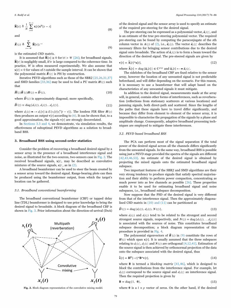
Consider the problem of recovering a broadband desired signal by asensor array in the presence of a broadband interference signal andnoise, as illustrated for the two-sources, two-sensors case in Fig. 2. Thereceived broadband signals, tx[ ], may be described as convolutivemixtures of the source signals, ts[ ], as in (2).

A broadband beamformer can be used to steer the beam created bya sensor array toward the desired signal. Range-bearing plots can thenbe produced using the beamformer output, from which the target'slocation can be gathered.

3.1. Broadband conventional beamforming

The broadband conventional beamformer (CBF) or tapped delayline (TDL) beamformer is designed to use prior knowledge to bring thedesired signal to broadside. A block diagram of the broadband CBF isshown in Fig. 3. Prior information about the direction-of-arrival (DoA)

of the desired signal and the sensor array is used to specify an estimateof the required pre-steering for the desired signal.

The pre-steering can be expressed as a polynomial vector, a z( )s , andis an estimate of the true pre-steering polynomial vector. The requiredpre-steering can be found by computing the paraconjugate of the sthcolumn vector in A z( ) of (2), i.e., a z( )∼

s . The vector a z( )s describes thenecessary filters for bringing sensor contributions due to the desiredsignal onto broadside. The action of a z( )s is to form a beam toward thedirection of the desired signal. The pre-steered signals are given by

t t tv A x[ ] = [ ]* [ ], (12)

where t tA a[ ] = diag{ [ ]} ∈sp p× and at za [ ] ∘—• ( )s s .

The sidelobes of the broadband CBF are fixed relative to the sensorarray, however the location of any unwanted signal is not predictablebeforehand, and will differ depending on the scenario. For this reason,it is necessary to use a beamformer that will adapt based on thecharacteristics of any unwanted signals it must mitigate.

In addition to the desired signal, measurements made at the arraywill, in general, contain other forms of interferences, such as reverbera-tion (reflections from stationary scatterers at various locations) andjamming signals, both direct-path and scattered. Since the lengths ofthe paths that these signals have to travel differ significantly, andbecause they differ from element to element of the sensor array, it isimpossible to characterise the propagation of the signals by a phase andamplitude change. Consequently, adaptive broadband processing tech-niques are employed to mitigate these interferences.

3.2. PEVD based broadband BSS

The PCA can perform most of the signal separation if the totalpower of the desired signal across all the channels differs significantlyfrom the unwanted signals. In the same way, broadband BSS is possibleusing just a PEVD stage provided the spectra of the signals are different[42,43,46,53]. An estimate of the desired signal is obtained byprojecting the mixed signals onto the estimated broadband signalsubspace.

Two important features of the SBR2 and SMD algorithms are theirvery strong tendency to produce signals that satisfy spectral majorisa-tion and their ability to perform power compaction, concentrating asmuch power into as few channels as possible [26]. These propertiesenable it to be used for estimating broadband signal and noisesubspaces, i.e., broadband subspace decomposition.

Now suppose that the PSD of the desired signal is very differentfrom that of the interference signal. Then the approximately diagona-lised CSD matrix in (10) and (11) can be partitioned as

D Nz d z d z z( ) = diag{ ( ), ( ), ( )},1 2 (13)

where d z( )1 and d z( )1 tend to be related to the strongest and secondstrongest source signals, respectively, and N z d z d z( ) = diag{ ( ), … ( )}p3is associated with the sources of noise. This constitutes broadbandsubspace decomposition; a block diagram representation of thisprocedure is provided in Fig. 4.

The polynomial eigenvectors of R z( ) in (9) constitute the rows ofH z( ) which span tx[ ]. It is usually assumed that the three subspacesrelating to d z( )1 , d z( )2 and N z( ) are orthogonal [4,12,41]. Estimation ofthe source signal is then achieved by orthonormal projection of the dataonto the subspace associated with the desired signal, thus

t t ts H B v^[ ] = [− ]* * [ ],H (14)

where B is termed a blocking matrix [41,46], which is designed toblock the contributions from the interference signal. For example, letd z( )1 correspond to the source signal and d z( )2 an interference signal.Then the required projection is given by

B 0= diag{1, }, (15)

where 0 is a p1 × vector of zeros. On the other hand, if the desiredFig. 2. Block diagram representation of the convolutive mixing model.

S. Redif et al. Signal Processing 134 (2017) 76–86

79

signal is very weak compared to the interference, which is often thecase for many practical problems, then a more appropriate blockingmatrix is

B 0= diag{0, 1, }. (16)

The operation in (14) can be viewed as being analogous to the PCAstage in BSS [1], and thus performing second-order broadband BSS onconvolutively mixed signals. Note, however, that it does not performunmixing in the conventional sense of compensating for the mixingimposed by the mixing matrix τA[ ] in (2). Instead, it representsseparation of the broadband signals from noise, such that the noisepower in ts [ ] is less than that in tx[ ] of (2). The procedure outlined hereconstitutes PEVD-based broadband BSS.

There are a number of applications where PEVD-based broadbandBSS can be employed. In the following we consider its application toknown problems in sonar detection and radar clutter mitigation.

3.3. PEVD based broadband adaptive beamforming

Application of a broadband adaptive beamformer (ABF) to theproblem outlined in Section 3.1 can yield better performance. The ABF

can modify the directivity of the sensor array such that the target returnis detected, and interferences and noise are suppressed.

As we have already discussed, the PEVD-based broadband BSSsystem in Fig. 4 can be used as part of an ABF system with the aim ofmitigating interference and noise. A possible PEVD-based ABF isshown in Fig. 5. The PEVD-based broadband ABF comprises threestages:

1. Interference mitigation: The PEVD-based broadband BSS describedabove is applied to suppress the effects due to interferences andnoise. Estimates of the broadband signal subspace (signal plus noisesubspace) and the noise subspace (interference plus noise subspace)of the input signals are obtained. Projection of the sensor signalsonto the estimated broadband signal subspace results in a significantreduction of energy due to the interference. The output signals fromthis process are ‘cleaned’ versions of the sensor signals.

2. Matched filtering: A receive filter that is matched to the desiredsignal is employed in order to further enhance the desired signal

Fig. 3. Block diagram of the broadband CBF – tapped-delay line beamformer.

Fig. 4. Flowchart of the power-based broadband BSS using PEVD.

Fig. 5. Block diagram of a PEVD-based broadband ABF.

S. Redif et al. Signal Processing 134 (2017) 76–86

80

[54]. For example, in underwater acoustics, a broadband pulsedchirp signal is usually used, so in this case the receive filter is chosensuch that it is matched to the transmitted chirp signal [55].

3. Broadband conventional beamforming: The output signals from thematched filter are likely to be spread over a wide frequencybandwidth. A pre-steering network is required to focus the phasedarray beam towards the direction of the desired signal. This can beachieved with the broadband CBF of Fig. 3.

3.4. Example problem I – underwater acoustics

Consider the scenario where a submarine is to be located using atowed array, as depicted in Fig. 6. The desired signal received by apassive array is a reflection from the target of the acoustic source signaltransmitted from the towed active array. The reflected signal is aDoppler-shifted version of the source signal. The passive array alsoreceives different time-delayed and attenuated versions of the sourcesignal from different paths due to a reverberant (multipath) environ-ment. This is usually in the presence of a strong broadband (jamming)signal produced by the submarine for concealment purposes; thissignal may also be received from different paths. The objective then isto determine the range and bearing of the target in this severeenvironment given measurements from the passive array.

The propagation of the signal sources to the passive array sensorsmay be represented in the form of (2). The polynomial mixing matrixA z( ) describes the convolutive nature of the channel, as well asencoding the contributions of the source signal to each sensor.

In order to test the PEVD-based broadband ABF described inSection 3.3, we have performed some computer simulations using realtrials data gathered from a towed array of p=40 hydrophones. Thetransmitted signal was a pulsed linear period modulated (LPM) signalwith a pulse length of 0.25 s and a pulse repetition interval (PRI) of15 s. For each PRI's worth of data a power response (range-bearingintensity map) of the beamformer was produced. The data is for thecase where a broadband source was used and a continuous-wave (CW)jamming signal was present. Note that, typically, there were two (man-made) sources, i.e., q=2: one corresponding to the pulsed LPM and theother related to the CW tone. However, there were sections of datawhere the jammer was switched off, in which case the transmitted LPMsignal was the only artificial source.

In Fig. 7(a), we show responses of the broadband CBF applied with12 uniformly spaced taps. Each plot is of range versus bearing obtainedby processing the data from a single PRI. From the response of thebroadband CBF we see that it is ineffective at localizing the target,especially when a broadband jamming signal is present (right). Thejamming signal appears at a single bearing (left hand side plot), but isspread over a large bandwidth, thus hiding the target return. Thestriation is due to leakage through the sidelobes of the broadband CBFresponse as the beam is scanned through azimuth.

The performance of the PEVD-based broadband ABF when appliedto the aforementioned sonar problem (Fig. 6) was evaluated bycomputer simulation and some results are presented here. InFig. 7(b), we show the range-bearing intensity map that results fromprocessing the data from a single PRI with the PEVD-based algorithm.Here the PEVD was obtained using the SBR2 algorithm. Also includedin the figure is the response of an IFB approach [56] in Fig. 7(c).

A striking result is that the effects caused by the jamming signal andreverberation are considerably attenuated with both the PEVD-basedbroadband ABF and the IFB approach for the problem considered. Forthe case where a jamming signal is present (right hand plots), thehighest intensity points on the range-bearing maps correspond to thetarget. For this data set, the PEVD-based broadband ABF methodappears to have suppressed the effects of the jamming signal and thereverberation slightly more than the IFB approach. Interestingly, in thecase where there is no jamming signal, the target appears clearer forthe plots generated using the PEVD-based broadband ABF comparedto the IFB method. This is because PEVD-based broadband ABF is ableto mitigate the effects due to the reverberation slightly better than theIFB approach.

It has been shown that the effects due to the reverberation may befurther attenuated by re-application of the PEVD-based broadband BSSstage in Fig. 4 to the cleaned sensor signals.

3.5. Example problem II – radar clutter suppression

In Fig. 8, an important example of the radar clutter suppressionproblem is illustrated. Simulation data was generated for this scenario.A moving radar device carrying an antenna some distance above aterrain surface is used to detect an airborne target. The radar antennais both a transmitter and a receiver oriented forward towards thedirection of travel. Regular successive pulse transmissions are madeilluminating the area of terrain bounded by the antenna beam.However, the rough terrain surface within the beam scatters the pulseenergy, a proportion of which is received back at the antenna after atime delay. The scattered return energy is termed clutter or backscatter.

The aim is to accurately estimate the DoA and Doppler frequency ofthe target in the presence of strong and dispersive backscatter from theground.

To this end, we applied the PEVD-based broadband ABF describedin Section 3.3 to simulated data, employing SMD to achieve thefactorisation in (10).

The role of the broadband beamformer is to adaptively suppress theradar clutter with little or no prior knowledge of the target signal or theclutter. In this light, it may be viewed as performing (second-order)BSS of broadband (convolutively mixed) signals. An estimate of theDoA and Doppler frequency of the target is then obtained with theapplication of a broadband CBF.

Our simulations were for three different scenarios each with atarget in the presence of clutter and additive white Gaussian noise; thesignal-to-noise ratio (SNR) of the target return in all of the datasets was0 dB. The target DoA is from an azimuth bearing of +16.7° and anelevation angle of −3.8°. The datasets correspond to the following threesimulated scenarios:

1. The target return is clear of the clutter in terms of Doppler shift at ahigher Doppler frequency (∼60 kHz) than the clutter.

2. The target return is in the sidelobe clutter at a lower Dopplerfrequency than the clutter at ∼46 kHz.

3. The target return is in the mainbeam clutter with the same Dopplerfrequency as the clutter, which is ∼54 kHz.

The simulated data is for a moving radar antenna with a 37 elementirregular array operating in a high pulse repetition frequency (PRF)mode. The PRF=263.8 kHz (2638 pulses) and there are four rangegates. For all datasets, the same clutter signal was used and the SNR of

Fig. 6. Example of sonar detection.

S. Redif et al. Signal Processing 134 (2017) 76–86

81

the clutter was much greater than that of the target return. The targetand clutter models used to produce the synthetic data are realistic,detail for which is beyond the scope of this paper.

In a practical radar system, the range of the target is tracked overtime, therefore, the range gate that contains the target return is knowna priori. The data from this range gate is collected for processing only.The attitude and height of the moving radar are unknown and its rangeto the target is also unknown.

In Figs. 9–11, graphs of azimuth versus Doppler frequency areshown, which are referred to as angle-Doppler, or bearing-Doppler,maps. For each figure, three angle-Doppler maps are shown; each is fora different elevation angle. The bar to the right of each plot relates theintensity of the returns to the colours used in the plot; the colour redsignifies a strong return, whereas blue indicates a weak return. Thegraphs shown are from images that have been decimated by ten (in thefrequency domain) and concentrated in the Doppler range 0–100 kHz.

As observed for the problem in Section 3.4, analysis of the broad-band CBF for this problem revealed that, for all three datasets, all of the

Fig. 7. Range-bearing plots for the (a) broadband CBF, (b) PEVD-based broadband ABF and (c) IFB approach applied to data with reverberation present and (left) no jamming signaland (right) with a strong jamming signal present.

Fig. 8. Example of radar detection.

S. Redif et al. Signal Processing 134 (2017) 76–86

82

apparent power was due to backscatter from the ground, the maximumof which was 1011. These results are not shown here.

The power response of the proposed PEVD-based broadband ABFto the input sensor signals, for all three data-set types, was analysed. Ingraphs (a), (b) and (c) of the figure, we show bearing-Doppler maps forelevation angles (a) −15°, (b) 0° (boresight), and (c) +15°, respectively.

For Fig. 9 it can be deduced that the algorithm has suppressed mostof the clutter energy. In particular, notice the reduction in clutterenergy at ∼50 kHz for an azimuth and elevation angle of, respectively,∼7° and 0o (i.e., boresight); in general, a reduction in clutter power of∼20 dB was achieved. With our prior knowledge of the location of thetarget, it is easy to see whether the algorithm has been able to extractthe target return. We observe that there is a concentration of energy ata Doppler frequency of 60 kHz that coincides with the target azimuthand elevation angles of +16.7° and −3.8°, respectively. This cannot beenergy due to backscatter since clutter does not exist in this azimuth-elevation plane for the given Doppler frequency. Therefore, we maydeduce from this that the energy concentration is related to the targetecho.

A similar level of success has been obtained after processing datasettype (2) – see Fig. 10. In Fig. 11, we show the results for the mostdifficult simulated scenario (3) (a target in the presence of mainbeamclutter). Here, there is very little or no energy related to the targetreturn, that is, the proposed algorithm cannot distinguish the targetecho from the backscatter.

Note that in situations where no prior knowledge of the targetlocation is available, it would be difficult to say with any certainty thatthe observed target return in Figs. 9 and 10 is the target, since there isstill a great deal of clutter power that the algorithm has failed to

remove. However, knowledge about the target's speed is usuallyavailable, and so assumptions regarding the required Doppler can bemade, which would improve target DoA estimates.

It has to be said that it was never expected that the proposedmethod would remove the clutter completely since it is operatingblindly. At this stage, our PEVD-based broadband ABF is considered asa possible pre-processing stage to post-Doppler space–time adaptiveprocessing.

In conclusion, we can say that in some cases the proposedtechnique can provide a good level of clutter suppression. However,the target echo cannot be identified with any degree of certaintybecause our results contain a significant amount of clutter residue.Further processing is required in order to achieve accurate localisationof the target. A possible idea for future work would be to investigate theperformance of the PEVD-based broadband ABF with Doppler filter-ing: the isolation of the Doppler bin of interest before narrowbandbeamforming is applied.

4. PEVD based broadband BSS using prior knowledge

Algorithms for BSS typically do not exploit prior information aboutthe desired signal nor do they make assumptions that focus attentionon the desired signal. As was demonstrated in Section 3, if the spectraof the source signals are different, then the PEVD carries out most ofthe separation. One way of incorporating prior knowledge into thePEVD-based BSS method of Section 3.2 is to emphasise the desiredsignal over the unwanted signals by utilizing prior information aboutthe desired signal.

Fig. 9. Angle-Doppler maps related to the output signals from the PEVD-based broad-band ABF for elevation angles (a) −15°, (b) 0°, and (c) +15°. The target can be correctlyidentified at a higher Doppler frequency than the clutter and at boresite elevation; sometarget return energy is also apparent at negative elevation angles. (For interpretation ofthe references to colour in this figure, the reader is referred to the web version of thispaper.)

Fig. 10. Angle-Doppler maps related to the output signals from the PEVD-basedbroadband ABF for elevation angles (a) −15°, (b) 0°, and (c) +15°. Target can becorrectly identified in the sidelobe clutter (for negative elevation angles) at a lowerDoppler frequency than the clutter. (For interpretation of the references to colour in thisfigure, the reader is referred to the web version of this paper.)

S. Redif et al. Signal Processing 134 (2017) 76–86

83

4.1. Domain-weighted broadband ABF

Different from the scheme shown in Fig. 5, the domain-weightedPEVD (DW-PEVD) [42] exploits knowledge about the desired-signalDoA in order to create a desired signal that is distinct from unwanted(interference) signals. This is achieved by manipulating the desiredsignal's energy.

With reference to the block diagram of DW-PEVD in Fig. 12, a fixedbeamformer, such as the broadband CBF in Section 3.1, is applied as afirst stage in order to bring the desired signal to broadside. As with thelast stage of the PEVD-based broadband ABF, knowledge about theantenna and the DoA of the desired signal can be used to perform pre-steering for the desired signal.

A generalised sidelobe canceller (GSC) beamformer as in [57] isthen applied, which comprises a quiescent vector and a blockingmatrix. A suitable quiescent vector designed to pre-steer the signalsto the desired DoA is applied, producing a primary channel. Thequiescent vector is used to compact power due to the desired signal atbroadside into the primary (first) channel; so most of the power relatedto the desired signal is contained in the primary channel. The columnsof the blocking matrix are designed as an orthonormal basis, spanningthe quiescent-vector null space, which define a set of p−1 auxiliarychannels.

The primary-channel signal is scaled by a domain-weightingconstant μ ∈ . Provided we have prior knowledge of the DoA of thedesired signal, we can ‘scale-up’ the primary-channel signal with μ > 1.This is the strategy adopted in our experiments to follow – see Section4.2. Note that the case μ=1 corresponds to the unmodified PEVD withno prior directional information. Also note that the domain-weightingcan be a filter, designed to exploit the temporal characteristics of the

desired signal, e.g., a matched filter. However, the performance of sucha method may depend to a significant extent on the accuracy ofinformation regarding the acoustic environment.

An iterative PEVD algorithm is then applied to strongly decorrelatea set of signals comprising the auxiliary channel and the emphasisedsignals. In [42], the SBR2 algorithm was successfully used for thispurpose.

Different from existing methods for robust broadband ABF, theDW-PEVD is based on a shift of paradigm away from adaptive noisecancellation toward broadband BSS. The adaptive filtering stage ofDW-PEVD is not based on least-squares power minimisation, and sodistinct from the GSC, which relies heavily on the availability of correctcalibration information. Any signal separation performed by DW-PEVD is done by transferring components of the desired and unwantedsignals between channels using a PU transformation, thus conservingthe total energy.

The basic philosophy behind DW-PEVD is to provide an extradegree-of-freedom represented by an appropriate choice of emphasistransformation to explore the region between the PEVD, which isentirely blind, and a fixed delay-and-sum beamformer which, beingnon-adaptive, relies entirely on prior knowledge of the steering vector.

4.2. Example problem – sensor arrays

To demonstrate the performance of DW-PEVD, results fromnumerical simulation of a broadband sensor array problem arepresented here. We model a desired signal impinging on a uniformlinear array in the presence of an interferer. The array is composed ofomnidirectional sensors, where p=10, with half-wavelength spacing.The DoA of the desired and interference signals are, respectively, −30°and +20°. An error in array calibration was introduced in the form of amismatch of +3° in the array response for the desired signal.

The desired signal was modelled as a pulse-shaped, zero-mean,quaternary phase shift keying (QPSK) signal, of which 2000 sampleswere used. The same model was used to produce the interferencesignal, except for the application of a different pulse shape. Sensornoise was modelled by zero-mean, unit variance complex Gaussianprocesses. Both the desired and interference signals had an SNR of0 dB.

In our experiments, PEVD factorisation was achieved using eitherthe SMD or SBR2C algorithms in [33,31], respectively; the algorithms

Fig. 11. Angle-Doppler maps related to the output signals from the PEVD-basedbroadband ABF for elevation angles (a) −15°, (b) 0°, and (c) +15°. There is no clearindication of a target from these results. The target return should be at the same Dopplerfrequency as the clutter and at a positive azimuth angle. (For interpretation of thereferences to colour in this figure, the reader is referred to the web version of this paper.)

Fig. 12. Block diagram representation of the domain-weighted PEVD method.

S. Redif et al. Signal Processing 134 (2017) 76–86

84

were allowed to run for 50 iterations. A scalar domain-weighting wasapplied as the primary enhancement, using only μ=1 or μ=2.

The power response of the overall system in Fig. 12 — convolutionof all transformations from sensors to the PEVD — is shown, for threeexperiments, in Figs. 13–15. Each plot in a figure shows the power ofthe beam (beampatterns), for different azimuthal angles of arrival andfrequency. The top two plots of each figure are the beampatterns for thefirst and second rows of the transform matrix, respectively, for thewhole DW-PEVD system. The third plot is an average beampatternover the rows 3 to p of the matrix. The bar to the right of each plotindicates power level in dBs; white signifies the highest power level,whereas black indicates the lowest power.

Fig. 13 is for the case where no primary enhancement was used, i.e.,μ=1. It is clear that the unweighted DW-PEVD cannot perform a goodlevel of signal separation since there is considerable leakage of the look-direction signal into the second channel and the interference signal intothe first channel. This is consistent with the theory presented earlier inthis section.

In Fig. 14, we show beampatterns for the beamformer with aprimary enhancement setting of μ=2 for the same scenario. We can seethat the DW-PEVD has designed a first beam which points to thedesired signal; the second beam, which is orthogonal to the first, isdesigned to point in the direction of the interferer. The other beams areorthogonal to the first two beams, as is indicated by very lowintensities.

We see that varying the value of μ provides an additional degree-of-

freedom for achieving good signal separation, and hence interferencesuppression. Simulation results from assessing the influence of μ haverevealed that the DW-PEVD performance has very little dependence onμ at large SNRs. These results are not provided here – the reader isreferred to [41] for a thorough characterisation.

In Fig. 15, beampatterns for a beamformer based on the subband-coding variant of SBR2, or the SBR2C algorithm, with a setting of μ=1,for the same scenario, is shown. Notice that even though there is noemphasis on the primary channel, the algorithm does fairly well inseparating the two signals, whilst also correctly identifying each signal'sDoA.

The improved performance is due to the fact that SBR2C isproportionately equally sensitive to changes in any of the signals[31,41]. While systems with a priori knowledge will usually performbetter, the SBR2C-based system is able to recover the signals and theirDoAs without this knowledge.

5. Conclusions

The overarching goal of this paper has been to build intuition andinsight into the important field of polynomial matrix decompositionsand its relevance to broadband BSS while leaving the detail toreferences.

Sample applications in the areas of broadband BSS and beamform-ing have been presented along with solutions and new results to threeimportant problems via a polynomial EVD based broadband beamfor-mer and a domain-weighted polynomial EVD. The results have beencompared to those of classical broadband methods, which highlightsthe suitability of the polynomial EVD to the problem of broadband BSS.

Acknowledgements

This work was supported in parts by the Engineering and PhysicalSciences Research Council (EPSRC) Grant number EP/K014307/1 andthe MOD University Defence Research Collaboration in SignalProcessing.

References

[1] P. Comon, Independent component analysis, a new concept?, Signal Process. 36(April (3)) (1994) 287–314.

[2] A. Hyvarinen, J. Karhunen, E. Oja, Independent Component Analysis, John Wileyand Sons, NY, 2001.

[3] G.H. Golub, C.F. Van Loan, Matrix Computations, 3rd edition, John HopkinsUniversity Press, Baltimore, Maryland, 1996.

[4] S. Haykin, Adaptive Filter Theory, 4th edition, Prentice Hall, Englewood Cliffs, NJ,2002.

Fig. 13. Beampatterns of the DW-PEVD using SMD, for the case whenSNR = INR = 0 dB and for μ=1.

Fig. 14. Beampatterns of the DW-PEVD using SMD, for the case whenSNR = INR = 0 dB and for μ=2.

Fig. 15. Beampatterns of the DW-PEVD using SBR2C, for the case whenSNR = INR = 0 dB and μ=1.

S. Redif et al. Signal Processing 134 (2017) 76–86

85

[5] J. Bobin, J.-L. Starck, M.J. Fadili, Y. Moudden, Sparsity and morphologicaldiversity in blind source separation, IEEE Trans. Image Process. 16 (November(11)) (2007) 2662–2674.

[6] J. Zhang, H. Zhang, L. Wei, Y.J. Wang, Blind source separation with patternexpression NMF, in: Advances in Neural Networks ISNN 2006, Springer-Verlag,Heidelberg, 2006, vol. 3971, pp. 1159–1164.

[7] A.S. Montcuquet, L. Hervé, F. Navarro, J.M. Dinten, J.I. Mars, Nonnegative matrixfactorization: a blind spectra separation method for in vivo fluorescent opticalimaging, J. Biomed. Opt. 15 (September (5)) (2010) 056009.

[8] B.M. Abadi, A. Sarrafzadeh, F. Ghaderi, S. Sanei, Semi-blind channel estimation inMIMO communication by tensor factorization, in: IEEE Workshop on StatisticalSignal Processing, August 2009, pp. 313–316.

[9] P.P. Vaidyanathan, Theory of optimal orthonormal subband coders, IEEE Trans.Signal Process. 46 (June (6)) (1998) 1528–1543.

[10] P. Smaragdis, Blind separation of convolved mixtures in the frequency domain,Neurocomputing 22 (1998) 21–34.

[11] S. Ikeda, N. Murata, A method of ICA in time–frequency domain, in: Workshop onIndependent Component Analysis and Signal Separation, 1999, pp. 365–370.

[12] H. Wang, M. Kaveh, Coherent signal-subspace processing for the detection andestimation of angles of arrival of multiple wide-band sources, IEEE Trans. Acoust.Speech Signal Process. 33 (August (4)) (1985) 823–831.

[13] H. Hung, M. Kaveh, Focussing matrices for coherent signal-subspace processing,IEEE Trans. Acoust. Speech Signal Process. 36 (August (8)) (1988) 1272–1281.

[14] Y. Bucris, I. Cohen, M.A. Doron, Bayesian focusing for coherent widebandbeamforming, IEEE Trans. Audio Speech Lang. Process. 20 (May (4)) (2012)1282–1296.

[15] T. Kailath, Linear Systems, Prentice Hall, Englewood Cliffs, NJ, 1980.[16] R.H. Lambert, M. Joho, H. Mathis, Polynomial singular values for number of

wideband source estimation and principal components analysis, in: Proceedings ofInternational Conference on Independent Component Analysis, 2001, pp. 379–383.

[17] R.H. Lambert, Multichannel blind deconvolution: FIR matrix algebra and separa-tion of multipath mixtures (Ph.D. thesis), University Southern California, LA, 1996.

[18] P.A. Regalia, P. Loubaton, Rational subspace estimation using adaptive losslessfilters, IEEE Trans. Signal Process. 40 (October (10)) (1992) 2392–2405.

[19] P.P. Vaidyanathan, Multirate Systems and Filter Banks, Prentice Hall, EnglewoodCliffs, 1993.

[20] P. Desarte, B. Macq, D.T.M. Slock, Signal-adapted multiresolution transform forimage coding, IEEE Trans. Inf. Theory 38 (March (2)) (1992) 897–904.

[21] P.A. Regalia, D.-Y. Huang, Attainable error bounds in multirate adaptive losslessFIR filters, in: Proceedings of IEEE Conference on Acoustics, Speech, and SignalProcessing, 1995, pp. 1460–1463.

[22] P. Moulin, M.K. Mihcak, Theory and design of signal-adapted FIR paraunitary filterbanks, IEEE Trans. Signal Process. 46 (April (4)) (1998) 920–929.

[23] B. Xuan, R.I. Bamberger, FIR principal component filter banks, IEEE Trans. SignalProcess. 46 (April (4)) (1998) 930–940.

[24] X. Gao, T.Q. Nguyen, G. Strang, On factorization of M-channel paraunitaryfilterbanks, IEEE Trans. Signal Process. 49 (July (7)) (2001) 1433–1446.

[25] J.G. McWhirter, P.D. Baxter, A novel technique for broadband SVD, in: 12thAnnual Workshop Adaptive Sensor Array Processing, MIT Lincoln Labs,Cambridge, MA, 2004.

[26] J.G. McWhirter, P.D. Baxter, T. Cooper, S. Redif, J. Foster, An EVD algorithm forpara-Hermitian polynomial matrices, IEEE Trans. Signal Process. 55 (May (5))(2007) 2158–2169.

[27] A. Tkacenko, P.P. Vaidyanathan, Iterative greedy algorithm for solving the FIRparaunitary approximation problem, IEEE Trans. Signal Process. 54 (January (1))(2006) 146–160.

[28] A. Tkacenko, Approximate eigenvalue decomposition of para-Hermitian systemsthrough successive FIR paraunitary transformations, in: IEEE InternationalConference on Acoustics Speech, and Signal Processing, March 2010, pp. 4074–4077.

[29] J.G. McWhirter, An algorithm for polynomial matrix SVD based on generalisedKogbetliantz transformations, in: European Signal Processing Conference, Aalborg,Denmark, 2010, pp. 457–461.

[30] J.A. Foster, J.G. McWhirter, M.R. Davies, J.A. Chambers, An algorithm forcalculating the QR and singular value decompositions of polynomial matrices, IEEETrans. Signal Process. 58 (March (3)) (2010) 1263–1274.

[31] S. Redif, J.G. McWhirter, S. Weiss, Design of FIR paraunitary filter banks forsubband coding using a polynomial eigenvalue decomposition, IEEE Trans. SignalProcess. 59 (November (11)) (2011) 5253–5264.

[32] S. Redif, S. Weiss, J.G. McWhirter, An approximate polynomial matrix eigenvaluedecomposition algorithm for para-Hermitian matrices, in: IEEE 11th InternationalSymposium on Signal Processing and Information Technology, Bilbao, Spain, 2011,

pp. 421–425.[33] S. Redif, S. Weiss, J.G. McWhirter, Sequential matrix diagonalisation algorithms

for polynomial EVD of parahermitian matrices, IEEE Trans. Signal Process. 63(January (1)) (2015) 81–89.

[34] S. Icart, P. Comon, Some properties of Laurent polynomial matrices, in: 9th IMAConference on Mathematics in Signal Processing, Birmingham, UK, December2012.

[35] S. Kasap, S. Redif, Novel field-programmable gate array architecture for computingthe eigenvalue decomposition of para-Hermitian polynomial matrices, IEEE Trans.Very Large Scale Integr. Syst. 22 (March (3)) (2014) 522–536.

[36] J. Corr, K. Thomson, S. Weiss, J.G. McWhirter, S. Redif, I.K. Proudler, Multipleshift maximum element sequential matrix diagonalisation for parahermitianmatrices, in: IEEE Workshop on Statistical Signal Processing, Gold Coast,Australia, July 2014, pp. 312–315.

[37] Z. Wang, J.G. McWhirter, J. Corr, S. Weiss, Multiple shift second order sequentialbest rotation algorithm for polynomial matrix eigenvalue decomposition, in: IEEEEuropean Signal Processing Conference, Nice, France, August 2015, pp. 844–848.

[38] M. Tohidian, H. Amindavar, A.M. Reza, A DFT-based approximate eigenvalue andsingular value decomposition of polynomial matrices, EURASIP J. Adv. SignalProcess. 1 (2013) 1–16.

[39] R. Brandt, M. Bengtsson, Wideband MIMO channel diagonalization in the timedomain, in: International Symposium on Personal, Indoor and Mobile RadioCommunications, 2011, pp. 1914–1918.

[40] J. Corr, K. Thompson, S. Weiss, I.K. Proudler, J.G. McWhirter, Shortening ofparaunitary matrices obtained by polynomial eigenvalue decomposition algorithms,in: 5th Conference of the Sensor Signal Processing for Defence, Edinburgh, UK,July 2015.

[41] S. Redif, Polynomial matrix decomposition and paraunitary filter banks (Ph.D.thesis), University of Southampton, 2006.

[42] S. Redif, J.G. McWhirter, P.D. Baxter, T. Cooper, Robust broadband adaptivebeamforming via polynomial eigenvalues, in: IEEE/MTS OCEANS'06, Boston, MA,September 2006, pp. 1–6.

[43] S. Redif, U. Fahrioglu, Foetal ECG extraction using broadband signal subspacedecomposition, in: IEEE Mediterranean Microwave Symposium, Guzelyurt,Cyprus, 2010. pp. 381–84.

[44] M.A. Alrmah, S. Weiss, S. Lambotharan, An extension of the MUSIC algorithm tobroadband scenarios using polynomial eigenvalue decomposition, in: 19thEuropean Signal Processing Conference, Spain, September 2011, pp. 629–633.

[45] M. Alrmah, S. Weiss, S. Redif, S. Lambotharan, J.G. McWhirter, M. Kaveh, Angle ofarrival estimation for broadband signals: a comparison, in: IET Intelligent SignalProcessing Conference, London, UK, December 2013.

[46] S. Redif, Fetal electrocardiogram estimation using polynomial eigenvalue decom-position, Turk. J. Electr. Eng. Comput. Sci. 24 (August (4)) (2014) 2483–2497.

[47] S. Weiss, S. Bendoukha, A. Alzin, F. Coutts, I. Proudler, J. Chambers, MVDRbroadband beamforming using polynomial matrix techniques, in: 23rd EuropeanSignal Processing Conference, Nice, France, September 2015, pp. 844–848.

[48] S. Weiss, S. Redif, T. Cooper, C. Liu, P. Baxter, J.G. McWhirter, Paraunitaryoversampled filter bank design for channel coding, EURASIP J. Appl. SignalProcess 2006 (2006) 1–10. http://dx.doi.org/10.1155/ASP/2006/31346 ID 31346.

[49] J. Foster, J. McWhirter, S. Lambotharan, I. Proudler, M. Davies, J. Chambers,Polynomial matrix QR decomposition for the decoding of frequency selectivemultiple-input multiple-output communication channels, IET Signal Process. 6(September (7)) (2012) 704–712.

[50] Z. Wang, J.G. McWhirter, S. Weiss, Multichannel spectral factorization algorithmusing polynomial matrix eigenvalue decomposition, in: Asilomar Conference onSignals, Systems, and Computers, 2015.

[51] S. Redif, S. Kasap, Novel reconfigurable hardware architecture for polynomialmatrix multiplications, IEEE Trans. Very Large Scale Integr. Syst. 23 (March (3))(2015) 454–465.

[52] P.D. Baxter, J.G. McWhirter, Robust adaptive beamforming based on domainweighted PCA, in: 13th European Signal Processing Conference, Antalya, Turkey,2005.

[53] G.D. Clifford, Singularvalue decomposition and independent component analysisfor blind signal separation, Bio Signal Image Process. 44 (6) (2005) 489–499.

[54] H.L. Van Trees, Detection, Estimation and Modulation Theory, Wiley & Sons Inc.,USA, 1968 ISBNs: 0-471-09517-6.

[55] J.-P. Hermand, W.I. Roderick, Acoustic model-based matched filter processing forfading time-dispersive ocean channels: theory and experiment, IEEE Trans. Ocean.Eng. 18 (October (4)) (1993) 447–465.

[56] R. Klemm, Space–Time Adaptive Processing Principles and Applications, Series 9,IEE Radar, Sonar, Navigation and Avionics, London, UK, 1998.

[57] L.J. Griffiths, C.W. Jim, An alternative approach to linearly constrained adaptivebeamforming, IEEE Trans. Antennas Propag. 30 (January (1)) (1982) 27–34.

S. Redif et al. Signal Processing 134 (2017) 76–86

86