relaxations for the dynamic knapsack problem with

RELAXATIONS FOR THE DYNAMIC KNAPSACK PROBLEMWITH STOCHASTIC ITEM SIZES

A ThesisPresented to

The Academic Faculty

by

Daniel Blado

In Partial Fulfillmentof the Requirements for the Degree

Doctor of Philosophy inAlgorithms, Combinatorics, and Optimization

School of Industrial and Systems EngineeringGeorgia Institute of Technology

May 2018

Copyright c© 2018 by Daniel Blado

RELAXATIONS FOR THE DYNAMIC KNAPSACK PROBLEMWITH STOCHASTIC ITEM SIZES

Approved by:

Dr. Alejandro Toriello, AdvisorSchool of Industrial and SystemsEngineeringGeorgia Institute of Technology

Dr. Robert FoleySchool of Industrial and SystemsEngineeringGeorgia Institute of Technology

Dr. Shabbir AhmedSchool of Industrial and SystemsEngineeringGeorgia Institute of Technology

Dr. Santosh VempalaCollege of ComputingGeorgia Institute of Technology

Dr. Santanu DeySchool of Industrial and SystemsEngineeringGeorgia Institute of Technology

Date Approved: 19 April 2018

ACKNOWLEDGEMENTS

First and foremost, I would like to thank my advisor Alejandro Toriello for all of his time,

encouragement, and guidance throughout my many years at Georgia Tech. I am grateful

for his patient mentorship in being an academic, as well as for helping me explore various

research paths and career options. His direction has been truly invaluable to me.

I thank my co-author Weihong Hu for being an integral part in the development of the

early parts of this thesis. I also wish to thank the members of my dissertation committee,

Shabbir Ahmed, Santanu Dey, Robert Foley, and Santosh Vempala, for taking the time to

help me defend my thesis. I especially thank Selvaprabu Nadarajah for serving as my thesis

reader. Additionally, I thank the National Science Foundation for their support.

Finally, I would like to thank my family, who have always been supportive and loving

in everything I pursue. I especially thank my parents for being great role models and their

constant motivation, and my brother Joem for exemplifying the importance of perseverance.

iii

TABLE OF CONTENTS

ACKNOWLEDGEMENTS . . . . . . . . . . . . . . . . . . . . . . . . . . . . . . iii

LIST OF TABLES . . . . . . . . . . . . . . . . . . . . . . . . . . . . . . . . . . vi

LIST OF FIGURES . . . . . . . . . . . . . . . . . . . . . . . . . . . . . . . . . . vii

SUMMARY . . . . . . . . . . . . . . . . . . . . . . . . . . . . . . . . . . . . . . viii

I INTRODUCTION . . . . . . . . . . . . . . . . . . . . . . . . . . . . . . . . 1

1.1 Literature Review . . . . . . . . . . . . . . . . . . . . . . . . . . . . . . 5

1.2 Problem Formulation . . . . . . . . . . . . . . . . . . . . . . . . . . . . 6

II SEMI-INFINITE BOUND . . . . . . . . . . . . . . . . . . . . . . . . . . . . 9

2.1 Primal Relaxation . . . . . . . . . . . . . . . . . . . . . . . . . . . . . . 13

2.2 A Stronger Relaxation of Pseudo-Polynomial Size . . . . . . . . . . . . . 17

2.3 Correlated Item Values . . . . . . . . . . . . . . . . . . . . . . . . . . . 20

2.4 Computational Experiments . . . . . . . . . . . . . . . . . . . . . . . . . 21

2.4.1 Bounds and Policies . . . . . . . . . . . . . . . . . . . . . . . . . 21

2.4.2 Data Generation and Parameters . . . . . . . . . . . . . . . . . . 23

2.4.3 Summary and Results . . . . . . . . . . . . . . . . . . . . . . . . 26

2.5 Discussion . . . . . . . . . . . . . . . . . . . . . . . . . . . . . . . . . . 29

III ASYMPTOTIC ANALYSIS: MCK BOUND VS. GREEDY POLICY . . . . 31

3.1 A Second Regime . . . . . . . . . . . . . . . . . . . . . . . . . . . . . . 39

3.2 Case Study: Power Law Distributions . . . . . . . . . . . . . . . . . . . . 44

IV QUADRATIC BOUND . . . . . . . . . . . . . . . . . . . . . . . . . . . . . . 47

4.1 Structural Properties . . . . . . . . . . . . . . . . . . . . . . . . . . . . . 48


4.3 Discussion . . . . . . . . . . . . . . . . . . . . . . . . . . . . . . . . . . 54

V A GENERAL ALGORITHM . . . . . . . . . . . . . . . . . . . . . . . . . . 58

5.1 Zero Capacity Case . . . . . . . . . . . . . . . . . . . . . . . . . . . . . 61

iv

5.1.1 Structure of the Optimal Policy . . . . . . . . . . . . . . . . . . . 61

5.1.2 A Closed Form for w∗M(0) . . . . . . . . . . . . . . . . . . . . . . 63

5.1.3 Submodularity of v∗M(0) . . . . . . . . . . . . . . . . . . . . . . . 65

5.2 The Algorithm . . . . . . . . . . . . . . . . . . . . . . . . . . . . . . . . 66


5.3.1 Heuristics . . . . . . . . . . . . . . . . . . . . . . . . . . . . . . 75

5.3.2 Discussion . . . . . . . . . . . . . . . . . . . . . . . . . . . . . . 77

VI CONCLUSIONS AND FUTURE WORK . . . . . . . . . . . . . . . . . . . 88

APPENDIX A — FULL DATA TABLES: CHAPTER 2 . . . . . . . . . . . . 90

APPENDIX B — FULL DATA TABLES: CHAPTER 3 . . . . . . . . . . . . 96

APPENDIX C — FULL DATA TABLES: CHAPTER 4 . . . . . . . . . . . . 99

APPENDIX D — FULL DATA TABLES AND AUXILIARY PLOTS: CHAP-TER 5 . . . . . . . . . . . . . . . . . . . . . . . . . . . . . . . . . . . . . . . 103

REFERENCES . . . . . . . . . . . . . . . . . . . . . . . . . . . . . . . . . . . . . 110

v

LIST OF TABLES

1 Summary of all tested instances, excluding PP bound and dual policy. . . . 27

2 Summary of instances selected for PP bound. . . . . . . . . . . . . . . . . 27

3 Summary Results - Power Law MCK . . . . . . . . . . . . . . . . . . . . 46

4 Summary Results - Ratios . . . . . . . . . . . . . . . . . . . . . . . . . . 54

5 Summary Results - Success Rates . . . . . . . . . . . . . . . . . . . . . . 55

6 10 Items Summary . . . . . . . . . . . . . . . . . . . . . . . . . . . . . . 79

7 20 Items Summary . . . . . . . . . . . . . . . . . . . . . . . . . . . . . . 79

8 30 Item Summary . . . . . . . . . . . . . . . . . . . . . . . . . . . . . . . 80

9 Small instances. . . . . . . . . . . . . . . . . . . . . . . . . . . . . . . . . 91

10 100 items, continuous distributions. . . . . . . . . . . . . . . . . . . . . . 92

11 100 items, discrete distributions. . . . . . . . . . . . . . . . . . . . . . . . 93

12 200 items, continuous distributions. . . . . . . . . . . . . . . . . . . . . . 94

13 200 items, discrete distributions. . . . . . . . . . . . . . . . . . . . . . . . 95

14 MCK Data, Power Law Distribution, 200-items or Less . . . . . . . . . . . 97

15 MCK Data, Power Law Distribution, 1000-items or More . . . . . . . . . . 98

16 Quadratic Variables Data, Small Instances. . . . . . . . . . . . . . . . . . . 100

17 Quadratic Variables Data, 20 Items, Correlated Values and Sizes. . . . . . . 101

18 Quadratic Variables Data, 20 Items, Uncorrelated Values and Sizes. . . . . 102

19 General Algorithm Performance Data, 10 Items . . . . . . . . . . . . . . . 104



vi

LIST OF FIGURES

1 Two-dimensional projection of possible inequality (4b) coefficients forq (vertical axis) versus right-hand side (horizontal axis) when Ai has aBernoulli distribution with parameter p. The thick solid line and black dotsrepresent all possible coefficient values, and the dark gray triangle representsthe convex hull of these values. This set does not include the white dot northe dashed line and is therefore not closed. . . . . . . . . . . . . . . . . . 15

2 20 Items - Distribution Variance vs. Relative Remaining Gap . . . . . . . . 80

3 20 Items - Fill Rate vs. Relative Remaining Gap . . . . . . . . . . . . . . . 81

4 20 Items - Initial Gap vs. Relative Remaining Gap . . . . . . . . . . . . . . 81

5 30 Items - Distribution Variance vs. Relative Remaining Gap . . . . . . . . 82

6 30 Items - Fill Rate vs. Relative Remaining Gap . . . . . . . . . . . . . . . 82

7 30 Items - Initial Gap vs. Relative Remaining Gap . . . . . . . . . . . . . . 83

8 10 Items: wU,σ Set Size Frequencies, Bernoulli . . . . . . . . . . . . . . . 85

9 10 Items: wU,σ Set Size Frequencies, Non-Bernoulli . . . . . . . . . . . . 86

10 20 Items: wU,σ Set Size Frequencies . . . . . . . . . . . . . . . . . . . . . 86

11 30 Items: wU,σ Set Size Frequencies . . . . . . . . . . . . . . . . . . . . . 87

12 20 Items - Distribution Variance vs. Relative Gap Closed Per Loop . . . . . 107

13 20 Items - Fill Rate vs. Relative Gap Closed Per Loop . . . . . . . . . . . . 107

14 20 Items - Initial Gap vs. Relative Gap Closed Per Loop . . . . . . . . . . 108

15 30 Items - Distribution Variance vs. Relative Gap Closed Per Loop . . . . . 108

16 30 Items - Fill Rate vs. Relative Gap Closed Per Loop . . . . . . . . . . . . 109

17 30 Items - Initial Gap vs. Relative Gap Closed Per Loop . . . . . . . . . . 109

vii

SUMMARY

We consider a version of the knapsack problem in which an item size is random and

revealed only when the decision maker attempts to insert it. After every successful insertion

the decision maker can choose the next item dynamically based on the remaining capacity

and available items, while an unsuccessful insertion terminates the process. We propose a

new semi-infinite relaxation based on an affine value function approximation, and show that

an existing pseudo-polynomial relaxation corresponds to a non-parametric value function

approximation. We compare both theoretically to other relaxations from the literature and

also perform a computational study. Our first main empirical conclusion is that our new

relaxation, a Multiple Choice Knapsack (MCK) bound, provides tight bounds over a variety

of different instances and becomes tighter as the number of items increases.

Motivated by these empirical results, we then provide an asymptotic analysis of MCK by

comparing it to a greedy policy. Subject to certain technical conditions, we show the MCK

bound is asymptotically tight under two distinct but related regimes: a fixed infinite sequence

of items under increasing capacity, and where capacity and the number of items increase

at their own separate respective rates. The distributions tested in the initial computational

study are consistent with such findings, and these results allow us to shift the focus towards

stochastic knapsack instances that have a smaller number of items available, i.e. when the

bound/policy gap starts to become a cause for concern.

We then examine a new relaxation that builds upon the value function approximation

that led to MCK. This bound is based on a quadratic value function approximation which

introduces the notion of diminishing returns by encoding interactions between remaining

items. We compare the bound to previous bounds in literature, including the best known

pseudopolynomial bound, and contrast their corresponding policies with two natural greedy

viii

policies. Our main conclusion here is that the quadratic bound is theoretically more efficient

than the pseudopolyomial bound yet empirically comparable to it in both value and running

time.

Lastly, we develop a finitely terminating general algorithm that solves the dynamic

knapsack problem under integer sizes and capacity within an arbitrary numerical tolerance.

The algorithm follows the same value function approximation approach as the MCK and

quadratic bounds, whereby, in the spirit of cutting plane algorithms, we successively im-

prove upon a changing value function approximation through both column and constraint

generation. We provide theoretical closed form solutions for the zero capacity case as well

as an extensive computational study for the general capacitated case. Our most recent main

conclusion is that the algorithm is able to significantly reduce the gap when the initial bounds

or heuristic policies perform rather poorly; in other words, the algorithm performs best when

we need it to the most.

ix

CHAPTER I

INTRODUCTION

The deterministic knapsack problem is one of the fundamental discrete optimization models

studied by researchers in operations research, computer science, industrial engineering,

and management science for many decades. It arises in a variety of applications, and also

appears as a sub-problem or sub-structure in more complex optimization problems and

algorithms. Relaxations of the knapsack problem have in particular been studied both as

benchmarks for the problem itself, and also within general mixed-integer programming to

derive valid inequalities. Work in this vein includes classical studies on valid inequalities

for the knapsack polytope, such as covers and lifted covers (see [36] and references therein),

and more recent results concerning extended formulations, relaxation schemes and extension

complexity, e.g. [7, 38].

Knapsack problems under uncertainty have also received attention, both to model

resource allocation applications with uncertain parameters, and also as substructures of more

general discrete optimization models under uncertainty, such as stochastic integer programs

[41]. Specifically, recent trends in both methodology and application have focused attention

on models in which the uncertain data is not revealed at once after an initial decision stage,

but rather is dynamically revealed over time based on the decision maker’s choices; such

models have applications in scheduling [14], equipment replacement [15] and machine

learning [21, 22, 31], to name a few.

The model we study here is a knapsack problem with stochastic item sizes and this

dynamic revealing of information: The decision maker has a list of available items, but only

has a probability distribution for each item’s size. Each size is revealed or realized only

after the decision maker attempts to insert it, and the insertion is successful (and the process

1

continues) only if the size is less than or equal to the remaining capacity in the knapsack.

This dynamic paradigm contrasts with more static approaches, such as a chance-constrained

model in which the decision maker chooses an entire set of items whose total size fits in the

knapsack with at least a pre-specified probability [19].

Providing the decision maker with the flexibility to observe sizes as they are realized

possibly increases the attainable expected value while satisfying the knapsack capacity with

certainty. However, this additional model flexibility also implies additional complexity from

both a practical and theoretical point of view; a feasible solution to this problem comes in

the form of a policy that must prescribe what to do under any potential circumstance, rather

than simply a subset of items. This additional difficulty has motivated work to both design

efficient policies with good performance, and also to devise reasonably tight, yet tractable

relaxations. Our results focus mostly on the latter question, and consist of the following

main contributions:

i) We introduce a semi-infinite relaxation, a Multiple-Choice Knapsack (MCK) bound,

for the problem under arbitrary item size distributions, based on an affine value

function approximation of the linear programming encoding of the problem’s dynamic

program. We show that the number of constraints in this relaxation is at worst

countably infinite, and is polynomial in the input for distributions with finite support

(assuming the distributions are part of the input).

ii) When item sizes have integer support, we show that a non-parametric value function

approximation gives the relaxation from [31], which has pseudo-polynomially many

variables and constraints.

iii) We theoretically and empirically compare these relaxations to others from the literature

and show that both are quite tight. In particular, our new relaxation is notably tighter

than a variety of benchmarks and compares favorably to the theoretically stronger

pseudo-polynomial relaxation when this latter bound can be computed.

2

iv) We prove the MCK bound is asymptotically optimal by comparing it to a natural

greedy policy under two distinct but related problem formulations: a fixed infinite

sequence of items under increasing capacity, and where capacity and the number of

items increase at their own separate respective rates. Although both cases are subject

to certain assumptions, the theory is consistent with the empirical results tested in the

initial computational experiments.

v) We introduce a quadratic relaxation that builds on MCK that encodes interactions

between remaining items, and show that it maintains polynomial solvability yet

empirically can be comparable to the best known pseudo-polynomial bound in both

value and running time.

vi) We prove supplementary results for the special case where the capacity is zero: that the

optimal value function is submodular, prove a straightforward optimal policy exists,

and that the variables corresponding to the optimal value function approximation have

closed form solutions.

vii) We develop a finitely terminating general algorithm that solves the dynamic knapsack

problem under integer sizes and capacity within an arbitrary numerical tolerance

using a dynamic value function approximation approach. We present both theoretical

analysis and an extensive computational study, and show that the algorithm is able

to significantly reduce the gap when the initial bounds or heuristic policies perform

rather poorly; in other words, the algorithm performs best when we need it to the

most.

Our computational studies employ a variety of policies related to or derived from various

relaxations. Our results also show that even quite simple policies perform very well,

especially as the number of items grows. More generally, our results may indicate a way to

derive relaxations for more complex stochastic integer programs with dynamic aspects, such

as those studied in [47].

3

The remainder of the paper is organized as follows. We follow this chapter with a brief

literature review and conclude with the general problem formulation and preliminaries.

Chapter 2 introduces the semi-infinite relaxation (also known as the Multiple-Choice Knap-

sack, or MCK, bound) and proves its structural results. Section 2.2 discusses deriving the

stronger relaxation when item sizes have integer support, while section 2.3 explains how to

extend our methods to a more general model where an item’s value may be stochastic and

correlated to its size. Finally, section 2.4 outlines the results of our empirical study, with

section 2.5 concluding. The Appendix contains detailed computational results.

Chapter 3 provides the asymptotic analysis of the MCK bound. The initial problem

formulation compares the ratio between the MCK bound and greedy policy under a fixed

infinite sequence of items and increasing capacity. Section 3.1 then reexamines the asymp-

totic property through a different formulation that decouples the growth rates of the number

of items and capacity; this allows us to determine when MCK is asymptotically optimal

regardless of the rate of capacity growth. We end the chapter with a computational study of a

particular item size distribution that does not satisfy a key assumption made in the analysis;

the Appendix contains detailed results.

Chapter 4 introduces a quadratic bound that builds on the value function approximation

that lead to the MCK bound. We first prove some results on its structure and solvability

and proceed with an empirical study. Section 4.3 discusses the computational results and a

follow-up experiment that highlights a set of distributions for which the Quad LP sees the

largest improvement. The chapter concludes with comments on its practicality compared to

the MCK and pseudo-polynomial bounds.

Chapter 5 provides an overview of a generalized algorithm that solves the original

dynamic knapsack problem within numerical tolerance, under the assumption that sizes

and capacity are integers. We first examine a problem reformulation based on our previ-

ous value function approximation approaches and introduce the main algorithm method.

Section 5.1 discusses supplemental results investigating the special case where capacity is

4

zero. Section 5.2 discusses the algorithm proper, including theoretical analysis regarding

its intermediate subproblems and eventual termination. We conclude the chapter with an

extensive computational study in Section 5.3.

1.1 Literature Review

In its full generality, this problem was first proposed and studied by [12, 14], though

earlier research had studied the problem specifically with exponential item size distributions

[15]. The computer science community has focused on problems of this kind, developing

bounding techniques and approximation algorithms; in addition to [12, 14], other results in

this vein include [6, 13, 21, 22, 31].

The knapsack problem and its generalizations have been studied for half a century or

more, with many applications in areas as varied as budgeting, finance and scheduling; see

[26, 33]. Knapsack problems under uncertainty have specifically received attention for

several decades; [26, Chapter 14] surveys some of these results. For general packing under

uncertainty see [13, 47]. As with optimization under uncertainty in general, models and

solution approaches can be split into those that choose an a priori solution, sometimes also

called static models [34], and models that dynamically choose items based on realized

parameters, also called adaptive [13, 14]. Different authors have also studied uncertainty in

different components of the problem. For example, a priori or static models with uncertain

item values include [10, 23, 35, 42, 44], static models with uncertain item sizes include

[18, 19, 27, 28], and [34] study a static model with uncertainty in both value and size.

Dynamic or adaptive models for knapsacks with uncertain item sizes include the previously

mentioned work [6, 12, 14, 15, 21, 22], while [25] study a dynamic model with uncertain

item values. Other variants include stochastic and dynamic models [29, 30, 37] in which

items are not available ahead of time but arrive dynamically according to a stochastic

process.

5

The idea of obtaining relaxations of dynamic programs using value function approxi-

mations in the Bellman recursion dates back to [40, 46]. The technique gained wider use

within the operations research community beginning with [1, 11], to obtain relaxations

and also corresponding policies. It has since then been applied in a variety of stochastic

dynamic programming models with discrete structure, such as inventory routing [2] and the

traveling salesman problem [45]. In particular, [45] also considers the inclusion of quadratic

variables to a previously affine approximation, a technique revisited when investigating

the new quadratic relaxation in Section 4. When item sizes have integer support, showing

the polynomial solvability of the quadratic bound is in part due to the framework [24]

provides on integer programs over monotone inequalities. To our knowledge, this work is

the technique’s first application for a stochastic knapsack model; as with many dynamic

programs, the model’s idiosyncratic state and action spaces require specific analysis to

derive the relaxations and the subsequent results.

For our stochastic knapsack problem variant of interest, the investigation of asymptotic

properties of relaxations via a comparison to a natural greedy policy introduced in [12,

14] was initially empirically suggested by computational studies in [8]. The information

relaxation duality techniques and results introduced in [5] verify the asymptotic nature of the

greedy policy and suggest a similar result for a bound stemming from perfect information

relaxation. Their problem formulation allows for both the number of items and capacity to

tend to infinity, as opposed to initially assuming a fixed infinite sequence of items; this paper

will consider both formulations.

1.2 Problem Formulation

Let N := 1, . . . ,n be a set of items. For each item i ∈ N we have a non-negative random

variable Ai with known distribution representing its size, and a deterministic value ci >

0. Item sizes are independent, and we can accommodate random values by using their

expectation, as long as size and value are independent for each item. Section 2.3 below

6

discusses how to extend our techniques to the case when an item’s size and value may be

correlated; see also [21, 22, 31]. We have a knapsack of deterministic capacity b > 0, and we

would like to maximize the expected total value of inserted items. An item’s size is realized

when we choose to insert it, and we receive its value only if the knapsack’s remaining

capacity is greater than or equal to the realized size. Given any remaining capacity s ∈ [0,b],

we may choose to insert any available item, and the decision is irrevocable; see [21, 22, 31]

for models that allow preemption. If the insertion is unsuccessful, i.e. the realized size is

greater than the remaining capacity, the process terminates.

The problem can be modeled as a dynamic program (DP). The classical DP formulation

for the deterministic knapsack [16] chooses an arbitrary ordering of the items and evaluates

them one at a time, deciding whether to insert each one or not. However, to respond to

realized item sizes it may be necessary to consider all available items together without

imposing an order. We therefore use a more general DP formulation with state space

given by (M,s), where ∅ 6= M ⊆ N represents items available to insert and s ∈ [0,b] is the

remaining knapsack capacity. The optimal expected value is υ∗N(b), where the optimal value

function υ∗ is defined recursively as

υ∗M(s) := max

i∈M

P(Ai ≤ s)(ci +E[υ∗M\i(s−Ai)|Ai ≤ s])

, (1)

and we take υ∗∅(s) := 0. The linear programming (LP) formulation of this equation system

is

minυ

υN(b) (2a)

s.t. υM∪i(s)−P(Ai ≤ s)E[υM(s−Ai)|Ai ≤ s]≥ ciP(Ai ≤ s),

∀ i ∈ N,M ⊆ N \ i,s ∈ [0,b](2b)

υ ≥ 0. (2c)

In this doubly infinite LP the domain of each υM : [0,b]→ R+ is an appropriate functional

space [4].

7

Notation To alleviate the notational burden in the remainder of the thesis, we identify

singleton sets with their unique element when there is no danger of confusion. We denote

an item size’s cumulative distribution function by Fi(s) := P(Ai ≤ s) for i ∈ N, and its

complement by Fi(s) := P(Ai > s). Similarly, the quantity Ei(s) := E[mins,Ai] is the

mean truncated size of item i∈N at capacity s∈ [0,b] [12, 14, 47], and features prominently

in our discussion. Intuitively, when the knapsack’s remaining capacity is s, we should not

care about item i’s distribution above s, since any realization of greater size results in the

same outcome – an unsuccessful insertion.

8

CHAPTER II

SEMI-INFINITE BOUND

The stochastic knapsack problem contains its deterministic counterpart as a special case,

and is therefore at least NP-hard. Moreover, [47] shows that several variants of the problem

are in fact PSPACE-hard. In general, therefore, we cannot expect to solve the LP (2) directly.

However, any feasible υ provides an upper bound υN(b) on the optimal expected value.

One possibility is to approximate the value function with an affine function,

υM(s)≈ qs+ r0 + ∑i∈M

ri, (3)

where r ∈RN∪0+ and q ∈R+. In this approximation, q is the marginal value of the remaining

knapsack capacity, r0 represents the intrinsic value of having the knapsack available, and

each ri represents the intrinsic value of having item i ∈M available to insert.

Proposition 2.0.1. The best possible bound given by approximation (3) is the solution of

the semi-infinite linear program

minq,r

qb+ r0 + ∑i∈N

ri (4a)

s.t. qEi(s)+ r0Fi(s)+ ri ≥ ciFi(s), ∀ i ∈ N,s ∈ [0,b] (4b)

r,q≥ 0. (4c)

Proof. Using (3),

υM∪i(s)−P(Ai ≤ s)E[υM(s−Ai)|Ai ≤ s]

= qs+ r0 + ∑j∈M∪i

r j−Fi(s)E[

q(s−Ai)+ r0 + ∑j∈M

r j

∣∣∣∣Ai ≤ s]

= qsFi(s)+qFi(s)E[Ai|Ai ≤ s]+ r0Fi(s)+ ri + Fi(s) ∑j∈M

r j

9

= qEi(s)+ r0Fi(s)+ ri + Fi(s) ∑j∈M

r j

≥ qEi(s)+ r0Fi(s)+ ri,

with equality holding when M =∅ or Fi(s) = 0.

Example 2.0.2 (Deterministic Knapsack). Suppose the item sizes are deterministic, so the

problem becomes the well-known deterministic knapsack. Let ai ∈ [0,b] be item i’s size; we

then have

qEi(s)+ r0Fi(s)+ ri =

qs+ r0 + ri, s < ai

qai + ri, s≥ ai.

When s < ai, constraints (4b) are dominated by non-negativity since ciFi(s) = 0, and hence

we can set r0 = 0. The constraints for all s≥ ai map to a single deterministic constraint, and

we obtain the LP

minq,r

qb+ ∑i∈N

ri

s.t. qai + ri ≥ ci, ∀ i ∈ N

r,q≥ 0.

This is the dual of the deterministic knapsack’s LP relaxation. Our bound therefore

generalizes this LP relaxation to the dynamic setting with stochastic item sizes.

To solve (4), we must efficiently manage the uncountably many constraints. For each

item i ∈ N, the separation problem is

maxs∈[0,b]

(r0 + ci)Fi(s)−qEi(s)

. (5)

The CDF Fi is upper semi-continuous, and the mean truncated size function Ei is continuous,

concave and non-decreasing, so the maximum is always attained. Efficient separation then

depends on the item’s distribution.

10

Proposition 2.0.3. If Fi is piecewise convex in the interval [0,b], we can solve the separation

problem (5) by examining only values corresponding to the CDF’s breakpoints between

convex intervals.

Proof. Because of the concavity of Ei, if Fi is convex, the most violated inequality will

always be at s ∈ 0,b. More generally, if the CDF is piecewise convex, within each convex

interval the most violated inequality will be at the endpoints.

Even if the CDF is not piecewise convex, it is almost everywhere differentiable [43,

Theorem 3.4]. Therefore, we can still partition [0,b] into at most a countable number of

segments within which it is either convex or concave. By Proposition 2.0.3, we only need

to check the endpoints of any convex segment. We may assume without loss of generality

that the CDF is differentiable within each concave segment (since otherwise we can further

partition the segment).

Proposition 2.0.4. Within a segment (s, s)⊆ [0,b] where Fi is concave and differentiable,

(5) can be solved by evaluating s, s and all solutions to

(r0 + ci)dds

Fi(s) = qFi(s) s ∈ (s, s). (6)

Proof. Let g(s) := (r0 + ci)Fi(s)−qEi(s). Then

g(s) = (r0 + ci +qs)Fi(s)−qFi(s)E[Ai|Ai ≤ s]−qs

= (r0 + ci +qs)Fi(s)−q∫ s

0adFi(a)−qs.

It follows that g is differentiable when Fi is differentiable. Deriving with respect to s,

dds

g(s) = (r0 + ci)dds

Fi(s)+qsdds

Fi(s)+qFi(s)−qsdds

Fi(s)−q

= (r0 + ci)dds

Fi(s)+qFi(s)−q = (r0 + ci)dds

P(Ai ≤ s)−qFi(s).

Even lacking piecewise convexity in the CDF, it may be possible to efficiently account

for all constraints. We discuss some specific distributions next.

11

Example 2.0.5 (Finite Distribution). Suppose Ai can take on a finite number of possible

values akKk=1, where 0 ≤ a1 < · · · < aK . In this case, the CDF is piecewise constant,

and thus piecewise convex, so the constraints can be modeled explicitly as long as K is

considered part of the problem input.

Example 2.0.6 (Uniform Distribution). Suppose Ai is uniformly distributed between [a, a],

where 0≤ a < a≤ b. (The requirement a≤ b is for ease of exposition.) Fi is again piecewise

convex, and we obtain

(r0 + ci)Fi(s)−qEi(s) =

−qs≤ 0, s ∈ [0,a)

1a−a

(12qs2 + s(r0 + ci−qa)+ 1

2qa2− (r0 + ci)a), s ∈ [a, a)

r0 + ci− 12q(a+a), s ∈ [a,b].

Therefore the most violated inequality is always at s ∈ 0, a. For s = 0, the inequality

is dominated by the non-negativity constraints, so we only need to add the constraint

12q(a+a)+ ri ≥ ci; we can once again set r0 = 0.

Example 2.0.7 (Exponential and Geometric Distributions). If Ai is exponentially distributed

with rate λ > 0, Fi is concave. Nevertheless, we get

(r0 + ci)Fi(s)−qEi(s) =(

r0 + ci−qλ

)(1− e−λ s),

which is maximized at s ∈ 0,b. As before, the case s = 0 is dominated by non-negativity,

so we only add the constraint 1λ

q(1− e−λb)+ r0e−λ s + ri ≥ ci(1− e−λb); it can be shown

that r0 = 0 here as well without loss of optimality. An analogous argument shows that only

the inequalities at s ∈ 0,b are necessary when Ai follows a geometric distribution.

Example 2.0.8 (Conditional Normal Distribution). Suppose Ai follows a normal distribution

with mean µ ≥ 0 and standard deviation σ > 0, conditioned on being non-negative. Fi is

then convex in [0,µ] and concave thereafter. Moreover, it is straightforward to see that

(r0 + ci)Fi(s)−qEi(s) is convex in [0,µ +qσ2/(r0 + ci)] and concave afterwards. Because

12

this function’s limit as s→ ∞ is r0 + ci−qE[Ai], it must be increasing in [µ +qσ2/ci,∞). It

follows that the most violated inequality is always at s∈ 0,b, so we only add the constraint

(4b) for s = b. As with the other examples where this is the only constraint needed, it can be

shown that r0 = 0 without loss of optimality.

The next example shows that r0 can drastically affect the bound given by (4).

Example 2.0.9 (Bernoulli Distribution). Suppose the knapsack has unit capacity, and each

item has unit value and size following a Bernoulli distribution with parameter p ∈ (0,1).

From Example 2.0.5, each item i has constraints only at s ∈ 0,1. Suppose we impose

r0 = 0; then for any n ≥ 1, the (restricted) optimal solution of (4) is ri = ciFi(0) = 1− p

for each i ∈ N and q = (1− ri)/Ei(1) = 1, yielding the objective ∑i∈N ri + q = 1+n(1− p).

On the other hand, the optimal value for any n is bounded above by the expected number of

Bernoulli trials before the second success, which is

p2∞

∑k=0

(k+1)2(1− p)k =2− p

p.

Once we include r0 in (4), the optimal solution becomes r∗0 = ciFi(0)/Fi(0) = (1− p)/p,

q∗ = ciFi(1)/Ei(1) = 1/p and r∗i = 0 for all i ∈ N, yielding an objective value of (2− p)/p,

which is asymptotically tight.

2.1 Primal Relaxation

The finite-support dual of (4) yields a “relaxed primal”, and gives further insight into the

approximation:

maxx ∑

i∈N∑

s∈[0,b]cixi,sFi(s) (7a)

s.t. ∑i∈N

∑s∈[0,b]

xi,sEi(s)≤ b (7b)

∑i∈N

∑s∈[0,b]

xi,sFi(s)≤ 1 (7c)

∑s∈[0,b]

xi,s ≤ 1, ∀ i ∈ N (7d)

13

x≥ 0, x has finite support. (7e)

This is a two-dimensional, semi-infinite, fractional multiple-choice knapsack problem [26],

also called a fractional knapsack problem with generalized upper bound constraints (see e.g.

[36]). The model has the following interpretation: For any feasible policy, xi,s represents

the probability the policy attempts to insert item i when s capacity remains; clearly, the

probability of attempting to insert i at any point cannot exceed 1 (7d). Similarly, there cannot

be more than one failed insertion (7c). Finally, for an attempted insertion, if the item’s size

exceeds the remaining capacity s, suppose we count this remaining capacity as a “fractional”

insertion; then the total expected size the policy inserts, including any “fractionally” inserted

size, does not exceed the knapsack’s capacity (7b).

Lemma 2.1.1. Problem (7) is a strong dual for problem (4).

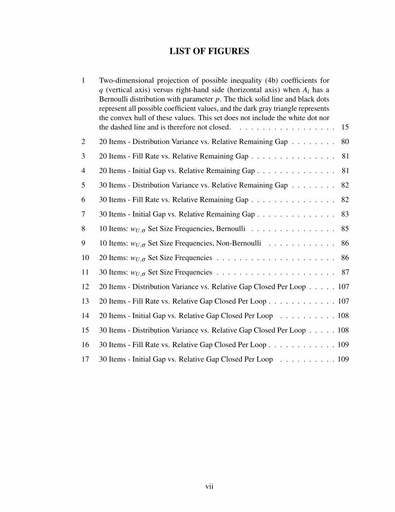
Proof. By [17, Theorems 5.3 and 8.4], (7) is a strong dual if the cone of valid inequalities

of (4), the characteristic cone, is closed. This cone is closed if for each i ∈ N the set

of inequalities implied by (4b) and the non-negativity constraints (4c) is closed. This is

equivalent to the following set being closed,

conv(

Ei(s), Fi(s),1,ciFi(s))

: s ∈ [0,b]+(θ ,0,0,0) : θ ≥ 0+(0,θ ,0,0) : θ ≥ 0

+(0,0,θ ,0) : θ ≥ 0+(0,0,0,−θ) : θ ≥ 0,

where the sum is a Minkowski sum. The first set in the sum, which we denote Q for

convenience, represents all non-trivial valid inequalities for item i ∈ N that do not weaken

any coefficient, re-scaled so ri’s coefficient is one. The remaining sets represent any potential

weakening of the inequality, either by increasing a left-hand side coefficient, or by decreasing

the right-hand side. Note that Q by itself is not necessarily closed; see Figure 1 for an

example. We will construct a convergent sequence in Q and show that its limit can be

achieved, perhaps by weakening a stronger inequality. For t ∈ N, let (ρ tk) and (st

k) for

k = 1, . . . ,4 respectively be a sequence of convex multiplier 4-tuples and knapsack capacity

14

Ei(s)

Fi(s)

p

1

(1, p)

1− p

(1− p, p)

Figure 1: Two-dimensional projection of possible inequality (4b) coefficients for q (verticalaxis) versus right-hand side (horizontal axis) when Ai has a Bernoulli distribution withparameter p. The thick solid line and black dots represent all possible coefficient values, andthe dark gray triangle represents the convex hull of these values. This set does not includethe white dot nor the dashed line and is therefore not closed.

4-tuples yielding a convergent sequence(∑k

ρtkEi(st

k),∑k

ρtkFi(st

k),1,ci ∑k

ρtkFi(st

k)

)→ (`q, `r0,1, `RHS) as t→ ∞.

(Q is at most three-dimensional, so each convex combination requires at most four terms.)

By iteratively replacing the sequence with a subsequence if necessary, we may assume

stk→ sk and ρ t

k→ ρk for each k. Then

`q = ∑k

ρkEi(sk), `r0 ≥∑k

ρkFi(sk) `RHS ≤ ci ∑k

ρkFi(sk),

where we respectively use the continuity, lower semi-continuity and upper semi-continuity

of Ei, Fi and Fi. We can then recover the limit inequality by weakening r0’s coefficient or

the right hand side if necessary.

We next compare (7) to a bound from the literature. The following linear knapsack

relaxation appeared in [14]:

maxx ∑

i∈Ncixi,bFi(b) (8a)

s.t. ∑i∈N

xi,bEi(b)≤ 2b (8b)

0≤ xi,b ≤ 1, i ∈ N. (8c)

15

Even though this formulation only has one variable per item, we keep the two-index notation

for consistency. The variables also have similar interpretations; xi,b in (8) represents the

probability that a policy attempts to insert an item at any point.

Theorem 2.1.2. The optimal value of (7) is less than or equal to the optimal value of (8).

Intuitively, (8) seems weaker because it must double the knapsack capacity. In fact, for

certain distributions, such as the ones covered in Examples 2.0.2, 2.0.6, 2.0.7 and 2.0.8, (7)

is simply (8) with the original capacity of b.

Proof. Multiplying constraint (7c) by b and adding it to constraint (7b), we can relax (7) to

maxx ∑

i∈N∑

s∈[0,b]cixi,sFi(s)

s.t. ∑i∈N

∑s∈[0,b]

xi,s(Ei(s)+bFi(s)

)≤ 2b

∑s∈[0,b]

xi,s ≤ 1, ∀ i ∈ N

x≥ 0, x has finite support.

The proof is finished by showing that Ei(s)+bFi(s)≥ Ei(b) for any s ∈ [0,b], because after

applying this further relaxation the optimal solution would have xi,s = 0 for s 6= b. Indeed,

Ei(s)+bFi(s) = Fi(s)E[Ai|Ai ≤ s]+ sFi(s)+b(Fi(s)− Fi(b)

)+bFi(b)

= Fi(s)E[Ai|Ai ≤ s]+ sFi(s)+b(Fi(b)−Fi(s)

)+bFi(b)

≥ Fi(s)E[Ai|Ai ≤ s]+(Fi(b)−Fi(s)

)E[Ai|s < Ai ≤ b]+bFi(b)

= Ei(b),

where in the inequality we use sFi(s)≥ 0 and b≥ E[Ai|s < Ai ≤ b].

Corollary 2.1.3 ([14, Theorem 4.1]). The multiplicative gap between the optimal value

of the stochastic knapsack problem υ∗N(b) and the bound given by (4) and (7) is at most

32/7≈ 4.57.

16

Example 2.0.2 shows that the relaxation (7) reduces to the deterministic knapsack’s LP

relaxation when item sizes are deterministic. This LP’s gap is well known to be two [26, 33],

and thus (7)’s gap cannot be less than two.

[14] also present a stronger polymatroid relaxation which has constraints similar to (8)

applied to every subset of items. We are not able to prove that (7) dominates this bound;

however, we discuss an empirical comparison of the two bounds in Section 2.4.

2.2 A Stronger Relaxation of Pseudo-Polynomial Size

Item sizes may have integer support in many cases. The knapsack capacity b can then be

taken to be integer as well, and it may be small enough that enumerating all possible integers

up to it is computationally tractable. If both assumptions hold, we can produce better value

function approximations of pseudo-polynomial size. For a state (M,s) with s ∈ Z+, consider

now the approximation

υM(s)≈ ∑i∈M

ri +s

∑σ=0

wσ , (9)

where r ∈ RN+ and w ∈ Rb+1

+ ; the ri’s have the same interpretation from before as intrinsic

values of each item, and each wσ represents the incremental intrinsic value of having σ

capacity left instead of σ−1. For a fixed M, this approximation allows a completely arbitrary

non-decreasing function of the capacity s; in particular, we can recover (3) by setting w0 = r0

and wσ = q for σ > 0, and this shows that (9) can produce a tighter relaxation.

Proposition 2.2.1 ([31]). The model

maxx ∑

i∈N

b

∑s=0

cixi,sFi(s) (10a)

s.t. ∑i∈N

b

∑s=σ

xi,sFi(s−σ)≤ 1, σ = 0, . . . ,b (10b)

b

∑s=0

xi,s ≤ 1, i ∈ N (10c)

x≥ 0 (10d)

17

gives an upper bound for the optimal value υ∗N(b) when item sizes have integer support.

The decision variables here have an identical interpretation to (7); xi,s is the probability

the policy attempts to insert item i when s capacity remains in the knapsack. The probability

of attempting to insert i still cannot exceed 1 (10c). Similarly, the σ -th unit of capacity can

be used at most once (10b). While this result is known from [31], our interpretation of the

bound as arising from the approximation (9) is new.

Proof. Substituting (9) into (2b), we obtain

υM∪i(s)−Fi(s)E[υM(s−Ai)|Ai ≤ s]

= ∑j∈M∪i

r j + ∑σ≤s

wσ −Fi(s) ∑j∈M

r j− ∑s′≤s

[(Fi(s′)−Fi(s′−1)

)∑

σ≤s−s′wσ

]= ri + Fi(s) ∑

j∈Mr j + ∑

σ≤swσ Fi(s−σ)≥ ri + ∑

σ≤swσ Fi(s−σ)≥ ciFi(s),

where as before the first inequality holds at equality when M = ∅ or Fi(s) = 0. The best

bound from an approximation given by (9) satisfying these conditions is thus

minr,w ∑

i∈Nri +

b

∑σ=0

wσ (11a)

s.t. ri +s

∑σ=0

wσ Fi(s−σ)≥ ciFi(s), i ∈ N,s = 0, . . . ,b (11b)

r,w≥ 0, (11c)

precisely the dual of (10). (Because item sizes have integer support, the number of constraints

in this model can be taken as finite, and thus classical LP duality applies.)

The interpretation of (10) via the value function approximation (9) also allows us to

compare it to another pseudo-polynomial bound from the literature. The following relaxation

appeared in [21, 22]:

maxx ∑

i∈N

b

∑s=0

cixi,sFi(s) (12a)

s.t. ∑i∈N

b

∑s=σ

xi,sEi(b−σ)≤ 2(b−σ), σ = 0, . . . ,b (12b)

18

b

∑s=0

xi,s ≤ 1, i ∈ N (12c)

x≥ 0. (12d)

Intuitively, this formulation applies the idea for (8) not only for the full capacity b, but also

by assuming the knapsack has σ fewer units of capacity for every σ = 0, . . . ,b.

Theorem 2.2.2. The optimal value of (10) is less than or equal to the optimal value of (12).

This theorem is a stronger version of a similar result in [31], which showed that (10) is

tighter than (12) in a worst-case sense.

Proof. Augment approximation (9) with redundant linear splines at every integer capacity,

yielding

υM(s)≈s

∑σ=0

qσ (s−σ)++ ∑i∈M

ri +s

∑σ=0

wσ ,

where q≥ 0. These new functions cannot improve the approximation, since for any M (9)

already captures an arbitrary non-decreasing function of capacity. Nevertheless, adding these

redundant variables makes the proof simpler. Following a similar argument to Propositions

2.0.1 and 2.2.1, this approximation results in the relaxation

maxx ∑

i∈N

b

∑s=0

cixi,sFi(s)

s.t. ∑i∈N

b

∑s=σ

xi,sEi(s−σ)≤ b−σ , σ = 0, . . . ,b

∑i∈N

b

∑s=σ

xi,sFi(s−σ)≤ 1, σ = 0, . . . ,b

b

∑s=0

xi,s ≤ 1, i ∈ N

x≥ 0,

which is equivalent to (10) because the first set of constraints is redundant. The proof now

follows by applying the argument from Theorem 2.1.2 to every σ = 0, . . . ,b.

19

2.3 Correlated Item Values

Our formulation so far only allows an item’s value to be random if it is independent of the

size, by using its expectation as a deterministic value. A more general setting studied in

the literature includes for each item i ∈ N a random value Ci that may be correlated to its

size Ai, where we now require knowledge of the joint distribution over (Ai,Ci). (Value-size

pairs remain independent across items.) To simplify exposition, we assume throughout this

section that each of these distributions has finite support.

Under these more general assumptions, the LP formulation (2) becomes

minυ

υN(b)

s.t. υM∪i(s)−Fi(s)E[υM(s−Ai)|Ai ≤ s]≥ Fi(s)E[Ci|Ai ≤ s],

∀ i ∈ N,M ⊆ N \ i,s ∈ [0,b]

υ ≥ 0,

and the DP recursion defining the optimal value function υ∗ is analogous. Similarly, the

value function approximations (3) and (9) remain the same, and yield analogous relaxations

to (7) and (10) respectively where the objective function coefficient for each variable xi,s

is now the item’s conditional expected value Fi(s)E[Ci|Ai ≤ s]. Assuming item sizes have

integer support, there is no substantive change to model (10), and this more general version

is already treated in [21, 22, 31].

For the affine approximation, however, the relaxation

maxx ∑

i∈N∑

s∈[0,b]xi,sFi(s)E[Ci|Ai ≤ s]

s.t. ∑i∈N

∑s∈[0,b]

xi,sEi(s)≤ b

∑i∈N

∑s∈[0,b]

xi,sFi(s)≤ 1

∑s∈[0,b]

xi,s ≤ 1, ∀ i ∈ N

20

x≥ 0, x has finite support,

has the slightly altered separation problem

maxs∈[0,b]

Fi(s)

(r0 +E[Ci|Ai ≤ s]

)−qEi(s)

for every item i ∈ N. Separation now also depends on the conditional expected value

function s 7→ Fi(s)E[Ci|Ai ≤ s]. If size-value pairs have finite support, this function is

piecewise constant, and its breakpoints occur in the same points as the CDF Fi. Therefore,

at optimality the relaxation will only have positive xi,s values for those s where Ai has

probability mass, just as in the case where value is deterministic.

2.4 Computational Experiments

We next present the setup and results of a series of experiments intended to compare the

upper bounds presented in the previous sections and benchmark them against various policies

related to the bounds.

2.4.1 Bounds and Policies

We first describe each of the bounds and policies we investigated. We tested the bounds

given by (7), which we refer to as MCK (for multiple-choice knapsack), and (10), which

we call PP (for pseudo-polynomial). To include a bound independent of our techniques,

we also computed a simulation-based perfect information relaxation (PIR) [9], obtained by

repeatedly simulating a realization of each item’s size and solving the resulting determin-

istic knapsack problem, then computing the sample mean of the optimal value across all

realizations; this estimated quantity is an upper bound because it allows the decision maker

earlier access to the uncertain data, i.e. it violates non-anticipativity. For this and all other

simulations we used 400 realizations. We did not include bounds (8) and (12) in light of

Theorems 2.1.2 and 2.2.2.

21

We also considered the following bound from [14]:

maxx ∑

i∈Ncixi,bFi(b)

s.t. ∑i∈J

xi,bEi(b)≤ 2b(

1−∏i∈J

(1− Ei(b)/b

)), J ⊆ N

0≤ xi,b ≤ 1, i ∈ N.

By employing an appropriate variable substitution, this LP can be recast as a linear poly-

matroid optimization problem and solved with a greedy algorithm. This bound clearly

dominates (8), and [14] also show that it has a worst-case multiplicative gap of 4 with the

optimal value υ∗N(b). We haven’t yet been able to show an analogue of Theorem 2.1.2, so

we planned to also include this bound in the experiments. However, after preliminary tests,

this bound did significantly worse than MCK; it was always at least 14% worse than the

best comparable bound (either MCK or PIR), and was often 40%-60% worse. We therefore

did not include it in the larger set of experiments.

As for policies, we considered several derived from the various bounds. Arguably

the simplest policy for this problem is a greedy policy, which attempts to insert items in

non-increasing order of their profitability ratio at full capacity, ciFi(b)/Ei(b), the ratio of

expected value to mean truncated size. In addition to its appealing simplicity, this policy is

motivated by various theoretical results. First, it generalizes the deterministic knapsack’s

greedy policy, which is well-known to have a worst-case multiplicative gap of 1/2 under a

simple modification [33]. Also, [15] showed that this policy is in fact optimal when item

sizes follow exponential distributions. Finally, [14] analyzed a modified version of it with a

simple randomization and showed that it achieves a worst-case multiplicative gap of 7/32

(this is the basis for the analysis of (8)). We also implemented an adaptive greedy version of

the policy that does not fix an ordering of the items, but rather at every encountered state

(M,s) computes the profitability ratios at current capacity ciFi(s)/Ei(s) for remaining items

i ∈M and chooses a maximizing item.

In addition to yielding bounds by restricting (2), the value function approximations

22

(3) and (9) can of course be used to construct policies, by substituting them into the DP

recursion (1). We refer to these two policies as the MCK and PP dual policies, to match the

bound names. The MCK dual policy uses an optimal solution (q∗,r∗) to (4) to choose an

item; at state (M,s), the policy chooses

arg maxi∈M

Fi(s)

(ci + r∗0 + ∑

k∈M\ir∗k +q∗

(s−E[Ai|Ai ≤ s]

)).

Similarly, the PP dual policy uses an optimal solution (r∗,w∗) to (11), and at state (M,s)

chooses

arg maxi∈M

Fi(s)

(ci + ∑

k∈M\ir∗k

)+

s

∑σ=0

w∗σFi(s−σ)

;

recall that this bound assumes item sizes have integer support.

Though we investigated both bounds, we did not implement the MCK dual policy,

because this policy actually exhibits quite undesirable behavior. Specifically, suppose item

sizes are deterministic; then (7) becomes the deterministic knapsack’s linear relaxation, and

its optimal solution has items set to 1 based on a non-increasing order of the deterministic

profitability ratio ci/ai, with at most one fractional item (the one that fills the knapsack’s

capacity). In this case, it is not difficult to show that the MCK dual policy is actually

indifferent between all items with positive value in the optimal solution of (7). While this

lack of distinction between items is not as problematic in the deterministic case (as all

items set to 1 would always fit), the policy exhibits analogous behavior for other item size

distributions for which (4) has r0 = 0 at optimality, such as uniform distributions, if all sizes

are less than b with certainty. This undesirable behavior was also reflected in preliminary

results, where the MCK dual policy performed poorly. We therefore did not include it in

further experiments.

2.4.2 Data Generation and Parameters

To our knowledge, there is no available test bed of stochastic knapsack instances; however,

there are various sources of deterministic instances or instance generators available. There-

fore, to obtain instances for our experiments, we used deterministic knapsack instances as a

23

“base” from which we generated stochastic instances. From each deterministic instance we

generated eight stochastic ones by varying the item size distribution and keeping all other

parameters. If a particular deterministic instance’s item i had size ai (always assumed to be

an integer), we generated the following four continuous distributions:

E Exponential with rate 1/ai.

U1 Uniform between [0,2ai].

U2 Uniform between [ai/2,3ai/2].

N Normal with mean ai and standard deviation ai/3, conditioned on being non-negative.

Similarly, we generated four discrete distributions:

D1 0 or 2ai each with probability 1/2.

D2 0 with probability 1/3 or 3ai/2 with probability 2/3.

D3 0 or 2ai each with probability 1/4, ai with probability 1/2.

D4 0, ai or 3ai each with probability 1/5, ai/2 with probability 2/5.

Note that all distributions are designed so an item’s expected size equals ai. Since the PP

bound and dual policy assume integer support, we could only test them on the second set of

instances. To ensure integer support for instances of type D2 and D4, after generating the

deterministic instance we doubled all item sizes ai and the knapsack capacity.

The deterministic base instances came from two data sources. We took eight small in-

stances from http://people.sc.fsu.edu/~jburkardt/datasets/knapsack_01/knapsack_

01.html; these range from five to twenty-five items. We generated 40 larger instances us-

ing the “advanced” instance generator from www.diku.dk/~pisinger/codes.html (see

[32]). The generator is a C++ script that takes in five arguments: number of items, range of

coefficients, type, instance number, number of tests in series. The last two input parameters

24

are used to adjust the problem fill rate, that is, the ratio between the sum of all item sizes

and capacity; we set these to maintain a fill rate in [2,5]. The “type” parameter refers to the

relationship between item sizes and profits. We used two types; in the first, sizes and values

are uncorrelated; in the second, sizes and values are “strongly correlated”. (The generator’s

authors observe that deterministic instances tend to be more difficult when sizes and values

are correlated.) We generated 10 uncorrelated instances with 100 items, 10 uncorrelated

instances with 200 items, 10 strongly correlated instances with 100 items, and 10 strongly

correlated instances with 200 items. For these 40 generated instances, we re-scaled the

capacity to 1000, and scaled and rounded the item sizes accordingly; we performed this

normalization for consistency, since the the dimension of (10) depends on the knapsack

capacity and thus influences the computing of the PP bound.

We used CPLEX 12.6.1 for all LP solves, running on a MacBook Pro with OS X 10.7.5

and a 3.06 GHz Intel Core 2 Duo processor. To estimate the PIR bound and all the policies’

expected values, we used the sample mean from 400 simulated knapsack instances. For all

tests on instances with the conditional normal distribution, we simulated sizes according to

a normal distribution with mean ai and standard deviation of ai/3. Whenever a simulated

item size was negative, we changed it to 0. Although this procedure does not exactly model

the conditional normal distribution, the changes in the simulated instances are minor given

that the probability of being non-negative is approximately 0.999.

We intended to test the PP bound and dual policy on all instances with discrete dis-

tributions, but encountered computational difficulty. Even for smaller instances, a naive

implementation of (10) would run out of memory. We therefore implemented a column

generation algorithm, but even this took a significant amount of time per instance. Roughly

speaking, D1 instances were the easiest to solve (usually between 60 and 90 minutes),

then D3 (120 to 150 minutes), then D2 (4.5 to 6.5 hours), and D4 instances were the most

difficult (12 to 16 hours or even more); the increased computation time required for D2 and

D4 instances can partly be explained by the need to double the knapsack capacity and thus

25

the number of variables and constraints. We therefore chose a subset of the instances to test;

of the small instances, we tested all except p08, since this instance has a very large capacity.

From the larger instances, we chose four each of the uncorrelated and strongly correlated

instances with 100 items. From all of these base instances, we tested the PP bound and dual

policy on all four discrete instance types, D1 through D4. Table 11 in the Appendix includes

computation times for the larger instances.

2.4.3 Summary and Results

Tables 1 and 2 contain a summary of our experiments for the different bounds and policies.

Table 1 excludes the PP bound and dual policy, but covers all tested instances, while Table 2

includes the PP bound and dual policy but covers only the instances in which these were

investigated. The tables are interpreted as follows. For each instance, we choose the smallest

bound as baseline, and divide all bounds and policy expected values by this baseline. The

first set of columns presents the geometric mean of this ratio, calculated over all instances

represented in that row. We show the ratios as percentages for ease of reading; thus, policy

ratios should be less than or equal to 100%, while bound ratios should be greater than or

equal to 100%. The one exception is the instances with exponentially distributed sizes

(type E); because we know from [15] that the greedy policy is optimal, we use this value

as a baseline. Also, for these instances the profitability ratio is invariant with respect to

remaining capacity, and thus the greedy and adaptive greedy policies are equivalent; hence

we do not report adaptive greedy performance for these instances.

For the second set of columns, we count the number of successes – one among the

bounds and one among the policies – and divide by the total number of instances represented

in that row. A success for a particular instance indicates the bound with the smallest ratio

and the policy with the largest ratio. If two ratios are within 0.1% of each other, we consider

them equivalent; thus, the presented success rates for each row do not necessarily sum to

100%.

26

Table 1: Summary of all tested instances, excluding PP bound and dual policy.Distribution Base PIR MCK Greedy Adapt. PIR Success MCK Success Greedy Success Adapt. Success

E small 147.59% 104.13% 100.00% - 0.00% 100.00% 100.00% -100cor 183.62% 100.07% 100.00% - 0.00% 100.00% 100.00% -100uncor 121.62% 100.55% 100.00% - 0.00% 100.00% 100.00% -200cor 188.47% 100.00% 100.00% - 0.00% 100.00% 100.00% -200uncor 121.90% 100.28% 100.00% - 0.00% 100.00% 100.00% -

U1 small 126.74% 100.37% 89.69% 89.31% 12.50% 87.50% 100.00% 87.50%100cor 154.20% 100.00% 98.78% 98.78% 0.00% 100.00% 100.00% 100.00%100uncor 111.28% 100.00% 99.07% 99.07% 0.00% 100.00% 100.00% 100.00%200cor 158.23% 100.00% 99.55% 99.56% 0.00% 100.00% 90.00% 100.00%200uncor 111.96% 100.00% 99.70% 99.70% 0.00% 100.00% 100.00% 100.00%

U2 small 112.55% 100.44% 86.95% 89.31% 12.50% 87.50% 12.50% 87.50%100cor 123.53% 100.00% 98.53% 98.65% 0.00% 100.00% 80.00% 100.00%100uncor 103.14% 100.00% 98.93% 99.36% 0.00% 100.00% 0.00% 100.00%200cor 126.15% 100.00% 99.20% 99.30% 0.00% 100.00% 60.00% 100.00%200uncor 103.23% 100.00% 99.44% 99.75% 0.00% 100.00% 0.00% 100.00%

N small 116.11% 100.32% 87.56% 89.48% 12.50% 87.50% 12.50% 87.50%100cor 126.58% 100.00% 98.81% 98.96% 0.00% 100.00% 50.00% 90.00%100uncor 104.31% 100.00% 99.14% 99.48% 0.00% 100.00% 0.00% 100.00%200cor 128.85% 100.00% 99.42% 99.53% 0.00% 100.00% 50.00% 100.00%200uncor 104.41% 100.00% 99.64% 99.90% 0.00% 100.00% 0.00% 100.00%

D1 small 111.00% 101.67% 75.04% 78.46% 50.00% 50.00% 12.50% 87.50%100cor 174.50% 100.00% 95.31% 97.15% 0.00% 100.00% 0.00% 100.00%100uncor 121.89% 100.00% 96.91% 97.85% 0.00% 100.00% 0.00% 100.00%200cor 180.87% 100.00% 97.70% 98.79% 0.00% 100.00% 0.00% 100.00%200uncor 124.18% 100.00% 98.55% 99.04% 0.00% 100.00% 0.00% 100.00%




Table 2: Summary of instances selected for PP bound.Distribution Base MCK Greedy Adapt. PP Dual Greedy Success Adapt. Success PP Dual Success

D1 small 109.57% 79.11% 82.82% 85.33% 0.00% 28.57% 71.43%100cor 100.00% 95.78% 97.59% 97.22% 0.00% 75.00% 25.00%100uncor 100.00% 97.22% 97.95% 95.24% 0.00% 100.00% 0.00%

D2 small 104.82% 86.40% 89.24% 87.98% 0.00% 42.86% 57.14%100cor 100.08% 97.37% 98.39% 97.84% 0.00% 75.00% 75.00%100uncor 100.05% 98.57% 99.29% 97.72% 0.00% 100.00% 0.00%

D3 small 104.65% 85.55% 89.42% 92.15% 0.00% 28.57% 85.71%100cor 100.01% 97.64% 98.70% 99.00% 0.00% 25.00% 75.00%100uncor 100.01% 98.26% 98.83% 97.63% 0.00% 100.00% 0.00%

D4 small 110.77% 88.09% 90.60% 91.14% 0.00% 28.57% 71.43%100cor 101.54% 96.98% 98.03% 97.90% 0.00% 75.00% 50.00%100uncor 100.76% 98.02% 98.43% 96.90% 0.00% 100.00% 0.00%

27

From the results we see that MCK is exclusively better than PIR in the summary statistics;

the success rates demonstrate that there are few cases in which PIR is better (mostly in the

small instances) but even here PIR is much worse than MCK on average. While PIR is

sometimes a good bound, e.g. for uncorrelated instances of type U2, it can often be much

worse than MCK, as much as 80% or 90% worse for correlated instances of type D4, for

example. We conjecture that MCK’s better performance is due in part to an averaging effect:

Assuming a large enough fill rate (recall the large instances maintain a fill rate between

2 and 5), individual items influence the solution less as the number of items increases.

Whereas MCK uses expected values, PIR is allowed to observe realizations and thus choose

each realization’s more valuable items. When the number of items is large, this additional

information may give the decision maker too much power and thus weaken the bound. It

is worth mentioning that the information relaxation techniques introduced in [9] suggest a

way to penalize PIR’s early observation of size realizations in order to improve the bound.

For this model, recent results in [5] indicate that when the penalty is chosen properly, the

resulting bound can be significantly tightened.

For the bounds reported in Table 2, we focus on comparing MCK to PP. We explain at

the start of Section 2.2 that PP is always less than or equal to MCK; therefore, we report here

only MCK as a percentage of PP. In contrast to the wide gaps we sometimes see between

PIR and MCK, MCK is very close to PP even though the latter bound employs a much

larger number of variables and constraints and is computationally much more demanding.

Interestingly, PP seems to offer the most benefit in smaller instances, where MCK can be

as much as 10% weaker on average. Conversely, the bounds are quite close in the larger

instances; MCK was within 1% of PP for all but one, where the gap was 1.54%. This seems

to match the original intent of PP, which was to consider instances in which b is small and

can be taken explicitly as part of the input [31].

As for policies, the adaptive greedy policy is in general better than the greedy policy.

Setting aside instances of type E, where greedy is optimal and the two are equivalent,

28

adaptive greedy is roughly equivalent to greedy for instances of type U1 and U2, and

noticeably better than greedy for type N and for all instances with discrete distributions.

This result is in line with what we expect, as adaptive greedy should be more robust to the

variation in realized item sizes. However, we also note that the gap between greedy and

adaptive greedy seems to decrease as the number of items increases; the experiments thus

suggest that the greedy policy is sufficient when the number of items is large enough. The

PP dual policy has mixed results compared to the greedy policies. It performs better than

adaptive greedy on small instances, but is worse on the larger instances, similarly to what

we see with the MCK and PP bounds.

In general, our results indicate that small instances might be harder, in the sense that

the simple MCK bound and greedy policies perform better as the number of items grows,

while the more complex PP bound and dual policy appear to offer the most benefit when

the number of items is small. Of course, if an instance is small enough, it may be possible

to directly solve the recursion (1), at least when sizes have integer support. It is thus in the

“medium” instance size range that PP may be most useful.

2.5 Discussion

We have studied a dynamic version of the knapsack problem with stochastic item sizes

originally formulated in [14, 15], and proposed a semi-infinite, multiple-choice linear

knapsack relaxation. We have shown how both this and a stronger pseudo-polynomial

relaxation from [31] arise from different value function approximations being imposed on

the doubly-infinite LP formulation of the problem’s DP recursion. Our theoretical analysis

shows that these bounds are stronger than comparable bounds from the literature, while our

computational study indicates that the multiple-choice knapsack relaxation is quite strong in

practice and in fact becomes tighter as the number of items increases.

Our results motivate additional questions. In particular, the fact that the simplest bound

and policy that we tested grow better as the number of items increases suggests it may

29

be possible to perform an asymptotic analysis of the two and perhaps show that they are

optimal as the item number tends to infinity, under appropriate assumptions; see Section 3

for such results. The recent results in [5], which appeared after our manuscript was initially

submitted, verify that this is indeed the case for the policy, and further suggest a similar

result is possible for the bound.

On the other hand, our results for the smaller instances also show that even the tightest

bound and best-performing policy can leave significant gaps to close. This motivates the

investigation of strengthened relaxations, perhaps analogously to a classical cutting plane

approach for deterministic knapsack problems. However, deriving such inequalities is

not obvious in our context. Finally, our techniques point to a general procedure to obtain

relaxations for dynamic integer programs with stochastic variable coefficients, such as the

multi-row knapsack models studied in [47].

30

CHAPTER III

ASYMPTOTIC ANALYSIS: MCK BOUND VS. GREEDY POLICY

We first define necessary terms and assumptions used in the analysis. The greedy ordering

[15] sorts items with respect to their value-to-mean-size ratio, ci/E[Ai], in non-increasing

order. The greedy policy attempts to insert items in this order until either all of the items

have successfully been inserted or an attempted insertion violates capacity.

Our analysis in this section slightly generalizes the original problem setup by assuming

the decision maker has access to an infinite sequence of items sorted according to the greedy

ordering; in other words, N = 1,2, . . . = N and ci/E[Ai] ≥ ci+1/E[Ai+1]. We can thus

study the asymptotic behavior of policy and bound as functions of capacity only. This

problem setup differs from results in [5], where the item set N also grows as part of the

analysis; our results are arguably stronger in the sense that they do not depend on the order

in which items become available to the decision maker (as the entire sequence is always

available). To further compare our techniques to [5], we include a second analysis under

their regime below in Section 3.1.

We must further clarify how we define v∗ for the infinite item case, as the original

formulation is defined recursively for finitely many items. Let v∗[n](b) and MCK[n](b) denote

the value function and MCK bound, respectively, with respect to the first n items according

to the greedy ordering. Note that both of these quantities are monotonically nondecreasing

sequences with respect to n, and for fixed b, v∗[n](b)≤MCK[n](b) holds for every n [8]. We

thus define v∗N(b) := limn→∞ v∗[n](b), and similarly define MCK(b) := limn→∞ MCK[n](b).

To show that both of these limits exist and are finite, it suffices to find a finite upper bound

for MCK[n](b) for all n; such a bound is provided below.

Let Greedy(b) refer to the expected policy value as a function of the knapsack capacity

31

b; note this is already well defined for the infinite item case since the greedy ordering is

assumed to be fixed. We use the greedy policy to show that MCK (7) is asymptotically tight;

in the process, this also proves that the greedy policy is asymptotically optimal, yielding an

alternate proof to [5]. To proceed with the analysis, we make the following assumptions.

Assumption 3.0.1. Among all items i,

i) expectation is uniformly bounded from above and below, 0 <¯µ ≤ E(Ai)≤ µ , and

ii) variance is uniformly bounded from above, Var(Ai)≤V ,

for some constants¯µ, µ,V .

Assumption 3.0.2. The sum of item values grows fast enough: ∑i≤k ci = Ω(k12+ε). For

example, having a uniform non-zero lower bound for all ci suffices.

Assumption 3.0.3.

c′0 := sups∈[0,∞)i=1,2,...

[E[Ai|Ai > s]− s

]< ∞. (13)

Intuitively, this last assumption governs the behavior of the size distributions’ tails; we

discuss some examples below.

We separate the analysis into four auxiliary results. The first result is a probability

statement used in later proofs.

Remark 3.0.4. Denote E[Ai] by the shorthand Ei. Then,

Ei− Ei(s)Fi(s)

= E[Ai|Ai > s]− s.

Proof. By definition,

Ei− Ei(s)Fi(s)

=Ei− (Fi(s)s+Fi(s)E[Ai|Ai ≤ s])

Fi(s)=

Ei−E[Ai|Ai ≤ s]Fi(s)

+(E[Ai|Ai ≤ s]− s).

The fraction in the right hand side above simplifies to

Ei−E[Ai|Ai ≤ s]Fi(s)

=(Ei−E[Ai|Ai ≤ s])Fi(s)

Fi(s)Fi(s)

32

=E[Ai|Ai ≤ s]Fi(s)(Fi(s)−1)+E[Ai|Ai > s]Fi(s)Fi(s)

Fi(s)Fi(s)

= E[Ai|Ai > s]−E[Ai|Ai ≤ s].

The second step establishes an upper bound for MCK.

Lemma 3.0.5. Let bk := ∑i≤kE[Ai]. Under Assumptions 3.0.1 and 3.0.3, for any n,

MCK[n](bk)≤∑i≤k

ciP(Ai ≤ bk)+ c0,

where c0 is a constant independent of k and n.

Proof. Fix k and n. Without loss of generality, we may assume n≥ k, since we can establish

the upper bound MCK[n](bk) ≤MCK[k](bk) for all n ≤ k. For the sake of brevity we will

abuse some notation in the proof, denoting bk as b (and E[Ai] as Ei). Recalling (4) is the

dual to the MCK bound (7), we proceed to find a dual feasible solution.

We start at the case i≥ k. Let us set ri = 0, which corresponds to allotting no value to

items after item k in the greedy ordering. We must satisfy

qEi(s)+ r0Fi(s)≥ ciFi(s), ∀s ∈ [0,∞).

Motivated by the possible case where Fi(s) = 1, if we set q = ck/Ek ≥ ci/Ei, variable r0

must now satisfy

r0Fi(s)≥ ciFi(s)−qEi(s) = ci− ciFi(s)−qEi(s)+( ck

Ek

)Ei−

( ck

Ek

)Ei

=[ci−

( ck

Ek

)Ei

]+

ck

Ek

[Ei− Ei(s)

]− ciFi(s).

Should Fi(s) = 0, the constraint reduces to 0 ≥ 0. Thus, assuming Fi(s) 6= 0, there are

three terms in the right hand side of the above inequality. Since r0 must upper bound such

constraints for all i and s, we drop the first and last terms, both of which are non-positive.

This yields constraints

r0 ≥ck

Ek

(Ei− Ei(s)Fi(s)

)=

ck

Ek

(E[Ai|Ai > s]− s

), ∀i≥ k, s ∈ [0,b], (14)

33

where the equality holds by Remark 3.0.4.

Next, we examine the case i < k. To find a valid choice of ri, we again are motivated by

the (possible) case where Fi(s) = 1, which implies

qEi(s)+ r0Fi(s)+ ri ≥ ciFi(s) =⇒ qEi + ri ≥ ci =⇒ ri ≥ ci−ck

EkEi.

This is a non-negative value for ri since the greedy ordering yields

ri = ci−ck

EkEi = Ei

[ ci

Ei− ck

Ek

]≥ 0.

These choices of q and ri present a dual objective of the desired form:

qb+ ∑i∈N

ri = b( ck

Ek

)+∑

i<kEi

( ci

Ei− ck

Ek

)= ∑

i<kci−∑

i<kEi

( ck

Ek

)+b( ck

Ek

)= ∑

i<kci−∑

i<kEi

( ck

Ek

)+∑

i≤kEi

( ck

Ek

)= ∑

i<kci +Ek

( ck

Ek

)= ∑

i≤kci = ∑

i≤kciFi(b)+∑

i≤kciFi(b).

Furthermore, noting that Fi(b) = P(Ai > bk) = P(Ai > ∑i≤kEi)≤ P(Ai > k¯µ)≤ Ei/k

¯µ ≤

µ/k¯µ , the sum ∑i≤k ciFi(b) can be upper bounded with

∑i≤k

ciFi(b)≤∑i≤k

c1Ei

E1Fi(b)≤

c1µ

¯µ

∑i≤k

Fi(b)≤c1µ2k

¯µ2k

=c1µ2

¯µ2 ,

which is constant with respect to k and i. Therefore, the second sum in the objective can be

upper bounded and absorbed into the c0 term.

It thus suffices to show that a valid choice for dual variable r0 exists such that it is

constant with respect to k (and bk), for then we can also absorb r0 into c0, completing the

proof. Continuing the case where i < k, the constraints in (4) require that r0 satisfy

r0Fi(s)≥ ciFi(s)− ri−qEi(s).

Should Fi(s) = 0, the choices of ri and q reduce the constraint to 0 ≥ 0. If Fi(s) 6= 0, the

condition is

r0 ≥ciFi(s)− ri−qEi(s)

Fi(s)=

ciFi(s)− ci +ckEiEk− ckEi(s)

Ek

Fi(s)

34

=−ciFi(s)+

ckEk[Ei− Ei(s)]

Fi(s)=−ci +

ck

Ek[E[Ai|Ai > s]− s],

where the last equality follows from Remark 3.0.4. This holds if r0 satisfies

r0 ≥ck

Ek[E[Ai|Ai > s]− s], ∀i ∈ [n],s ∈ [0,b],

which is exactly constraint (14) in the case that i≥ k. Recalling Assumption 3.0.3, setting

r0 = c1c′0/E1 satisfies (14) for all values of i and s. Since r0 is constant with respect to k and

n (and bk), we can set c0 = c1(µ2/

¯µ2 + c′0/E1). This result holds for all n, completing the

proof.

The above result proves that the limit MCK(bk) exists and is finite. Let Sk denote the

sum of the first k sizes according to the greedy ordering, Sk := ∑i≤k Ai. The expected

value of the greedy policy when restricted to the first k items under capacity bk is trivially

∑i≤k ciP(Si ≤ bk). This is a lower bound for the actual greedy policy, which considers all

of the items instead of the first k. By Lemma 3.0.5, for each bk we have a lower bound of

Greedy(bk)

MCK(bk)≥ ∑i≤k ciP(Si ≤ bk)

∑i≤k ciP(Ai ≤ bk)+ c0.

The ratio in the left-hand side above is always at most 1 since the numerator is a feasible

policy and the denominator is an upper bound on the optimal policy. We next examine the

asymptotic nature of the lower bound.

Lemma 3.0.6. Under Assumptions 3.0.1 and 3.0.2,

limk→∞

∑i≤k ciP(Si ≤ bk)

∑i≤k ciP(Ai ≤ bk)+ c0= 1.

Proof. It suffices to show that the numerator can be lower bounded by ∑i≤k ci−O(√

k), as

the result will then follow from Assumption 3.0.2 and the trivial upper bound P(Ai≤ bk)≤ 1.

Recalling bk = ∑i≤k

Ei = E[Sk], we first upper bound the probability

P(Si > bk) = P(Si−E[Si]> E[Sk−Si])≤ P(|Si−E[Si]|> E[Sk−Si])

35

= P((Si−E[Si])2 > (E[Sk−Si])

2)≤ Var(Si)(∑

i< j≤kE[Ai]

)2 ≤iV

(k− i)2

¯µ2 , (15)

where the second inequality comes from Markov’s (or Chebyshev’s) inequality. Next,

we define upper bound c := c1µ/E1 ≥ ci. Let j be some number such that j < k, to be

determined. Using (15) yields

∑i≤k

ciP(Si ≤ bk) = ∑i≤ j

ciP(Si ≤ bk)+ ∑j<i≤k

ciP(Si ≤ bk)

≥∑i≤ j

ci

[1− iV

(k− i)2

¯µ2

]+ ∑

j<i≤kci(1−P(Si > bk))≥∑

i≤kci−

cV

¯µ2 ∑

i≤ j

i(k− i)2 − c(k− j)

≥∑i≤k

ci−cV

¯µ2

j+1∫0

x(k− x)2 dx− c(k− j) = ∑

i≤kci−

cV

¯µ2

[ j+1k− j−1

+ ln(k− j−1)− lnk]− c(k− j)

= ∑i≤k

ci−cV

¯µ2

[k−√

k√k

+ ln(√

k)− lnk]− c(√

k+1) = ∑i≤k

ci−O(√

k).

The second to last equality occurs when we make the suitable choice k− j−1 =√

k, that is,

j = k−√

k−1. Letting (k− j−1) be of order√

k consequently minimizes the order of the

second and third terms (those that are not ∑i≤k ci) to be of order√

k; one can easily check

that choosing a different power of k will lead to an overall higher order for either the second

term or third term.

Lemma 3.0.6 examines the limit in terms of the number of items in the knapsack, a

discrete sequence dependent on k, but we wish to show the asymptotic property over all

positive values b. Therefore, we formalize this result in terms of the increasing knapsack

capacity b.

Theorem 3.0.7. Suppose we are given a greedily ordered infinite sequence of items satisfying

Assumptions 3.0.1, 3.0.2, and 3.0.3. Then,

Greedy(b)MCK(b)

→ 1 as b→ ∞. (16)

Proof. Given b, let bk− and bk+ refer to the nearest bk values below and above b, respec-

tively. Then, trivially Greedy(b)≥ Greedy(bk−). Further, MCK(b)≤MCK(bk+) since the

36

objective of MCK is nondecreasing with b. Therefore we obtain

Greedy(b)MCK(b)

≥Greedy(bk−)

MCK(bk+)≥

Greedy(bk−)

MCK(bk−)+ ck+Fk+(bk+)≥

Greedy(bk−)

MCK(bk−)+ c0→ 1.

The second inequality follows from decomposing the upper bound of MCK(bk+) into the

upper bound of MCK(bk−) and the additional objective term involving item k+, while the

last inequality follows because every ciFi(b) term can be upper bounded by a constant, as in

the proof of Lemma 3.0.6. The final expression goes to 1 by Lemma 3.0.6.

This result is consistent with the computational experiments in [8] that spurred our

analysis, which tested the MCK bound under the following distributions: bounded discrete

distributions with two to five breakpoints, uniform, and exponential. Under all such distribu-

tions, the data suggested that MCK and Greedy were asymptotically equivalent; comparing

with Assumption 3.0.3:

• Under the discrete and uniform distributions, the sizes exhibit uniformly bounded

support. Thus, the value c′0 defined in Assumption 3.0.3 exists and is finite (it is

simply the upper bound on item size support), and the theorem applies.

• Under the exponential distribution, suppose E[Ai] = 1/λi. By the memoryless property,

for any i and any s,

E[Ai|Ai > s]− s = (1/λi + s)− s = 1/λi < ∞.

Thus, if the item sizes have a uniformly bounded mean, c′0 exists and is finite, and the

theorem applies.

According to the analysis in the proof of Lemma 3.0.6, if the sum of the item values

grows as Ω(g(k)), the numerator of the fraction is lower bounded by Ω(g(k)−√

k); hence,

the rate of convergence is O(√

k/g(k)). For example, if g(k) = k, the rate of convergence is

O(k−1/2).

Corollary 3.0.8. The rate of convergence of (16) is O(√

k/g(k)), where ∑i≤k ci = Ω(g(k)).

37

Assumption 3.0.3 is not always straightforward to check for a particular distribution, so

we provide an alternate set of sufficient conditions.

Proposition 3.0.9. Suppose the following hold:

i) Among those items with bounded support, there exists a uniform finite upper bound.

ii) Among all items i without bounded support, there exists an α > 0 such that

(a) P(Ai > t)≥ e−αt for all t > 0, and

(b) Mi(α) := E[eαAi] ≤M(α) < ∞; that is, the moment generating function at α

exists and is uniformly bounded among such i.

iii) For all i, P(Ai > 0)≥ z > 0. Note that for continuous distributions we can trivially

take z = 1 since Ai is nonnegative.

Then,

c′0 = sups∈[0,∞)i=1,2,...

[E[Ai|Ai > s]− s

]< ∞.

Proof. There are three cases for each item: an item has bounded support, unbounded support

and zero probability of being 0, or unbounded support and nonzero probability of being 0.

For each case we exhibit a uniform bound across all items of that case, then set c′0 to the

maximum of these three absolute upper bounds.

The bounded support case is taken care of by the first condition. For the second case,

consider any item i. Since Ai is a nonnegative random variable, by Markov’s inequality

P(Ai > t) = P(eαAi > eαt)≤ E[eαAi]

eαt .

Further, recall for nonnegative random variables the identity E[Ai] =∫

∞

t=0 F(t)dt. Thus, for

the random variable (Ai− s),

E[Ai− s|Ai > s] =∫

∞

t=0P(Ai− s > t)dtP(Ai > s)

≤ 1P(Ai > s)

∫∞

t=0

E[eαAi]

eα(t+s)dt

38

=E[eαAi]

P(Ai > s)eαs

( 1α

)≤ M(α)

e−αseαs

( 1α

)=

M(α)

α< ∞.

The first inequality follows from the Markov bound presented earlier on P(Ai > t + s), while

the second inequality follows from both parts of the second assumption. This provides an

absolute upper bound for E[Ai− s|Ai > s] for all values of s ∈ (0,∞), taking care of the

second case of items.

For the third case of items, it suffices to uniformly bound the case that s = 0. By the

third assumption (and earlier assumption of uniformly bounded mean) we have

E[Ai−0|Ai > 0] =E[Ai]

P(Ai > 0)≤ µ

z< ∞.

Since the above analysis does not depend on the choice of i, this completes the proof.

3.1 A Second Regime

The results in [5] provide an alternate asymptotic analysis of the greedy policy in which

items become available to the decision maker incrementally as capacity grows; when the

number of items k grows, each new item is added to the same subset of already available

items. The authors examine an upper bound based on information relaxation techniques, and

provide a case analysis dependent on the growth of capacity as a function of the number of

available items, to show under what conditions the greedy policy is asymptotically optimal.

Motivated by this result, we show that the MCK bound allows for similar conclusions.

Consider denoting Greedy(k,b(k)) as the expected value gained from the greedy policy

given k items and b(k) capacity; we now make explicit the fact that b is a function of k.

Similarly, let MCK(k,b(k)) be the optimal value of MCK given k items and b(k) capacity.

Unlike the previous framework, we no longer make any assumption about the ordering

of items, implying in particular that items are possibly re-sorted for each k to calculate

Greedy(k,b(k)). We must therefore also make an additional assumption.

Assumption 3.1.1. The value-to-mean-size ratios are uniformly bounded from above,

ci/Ei ≤ r, for some constant r.

39

This assumption is satisfied if the items are sorted in the greedy order, as discussed in

the proofs of Lemma 3.0.6 and Theorem 3.0.7.

Theorem 3.1.2. Let f (k) be a non-negative, monotonically increasing function satisfying

f (k)→ ∞ as k→ ∞. If Assumptions 3.0.1 and 3.1.1 hold,

limk→∞

Greedy(k,b(k))MCK(k,b(k))

= 1

under any of the following conditions:

(a) Capacity scales as b(k) = ∑i≤kEi = Θ(k) (linearly), and ∑i≤k ci = Ω(k12+ε).

(b) Capacity scales as b(k) = ∑i≤ f (k)Ei = Ω(k) ( f (k) is superlinear), and ∑i≤k ci =

Ω(k12+ε).

(c) Capacity scales as b(k) = ∑i≤ f (k)Ei = o(k) ( f (k) is sublinear),

∑i≤ f (k)

ci = Ω([max f (k)/ f (√

k), f (√

k)]1+ε),

ln f (k) = o(max f (k)/ f (√

k), f (√

k)), and the following weaker version of

Assumption 3.0.3 holds:

sups∈[0,∞)

i=1,2,...,k

[E[Ai|Ai > s]− s

]= o( f (k)). (17)

In the above summations, indices i are ordered according to the greedy ordering for any

given k.

For comparison, in [5] the authors state that their assumptions are difficult to verify, and

provide sufficient conditions that are very similar to our assumptions here. For example,

they assume uniformly bounded means and variances, as in Assumption 3.0.1. Both results

assume similar uniform upper bounds on the value-to-mean-size ratios. Our only additional

assumptions lower bound the item mean sizes and the growth rate of the sum of item values.

40

Proof. The proof is similar to the proof of Theorem 3.0.7. It suffices to show that the limit

of the ratio is lower bounded by a quantity that goes to 1. Prior to examining each case

individually, we observe that under k items, the capacity is

b(k) = ∑i≤ f (k)

Ei = E[S f (k)] = Θ( f (k)),

where the linear case sets f (k) = k. With this in mind, the linear case reduces to the case

where b(k) = ∑i≤kEi = E[Sk], the same as in Lemma 3.0.6. Since we now limit the number

of items to k (as opposed to an infinite sequence of items), the bounds

Greedy(k,b(k))≥∑i≥k

ciP(Si ≤ b(k)), and MCK(k,b(k))≤∑i≤k

ciP(Ai ≤ b(k)),

now trivially hold. The Greedy upper bound actually holds at equality by definition of

the policy, while the MCK upper bound follows from the (possibly infeasible) solution

xi,b(k) = 1 for all i. (This takes advantage of the monotonicity of CDFs, and the fact that

there are only at most k items in the objective.) Thus we have

limk→∞


≥ limk→∞

∑i≤k ciP(Si ≤ E[Sk])

∑i≤k ciP(Ai ≤ E[Sk])= 1,

where the last inequality follows from Lemma 3.0.6, setting constant c0 to 0. (This shows

that the main difficulty for the first regime is finding an additional constant c0 to deal with

items i > k.)

For the superlinear case, we have f (k)≥ k for large enough k, and so

P(Si > b(k)) = P(Si > E[S f (k)])≤ P(Si > E[Sk]).

Therefore,


=Greedy(k,E[S f (k)])

MCK(k,E[S f (k)])≥

∑i≤k ciP(Si ≤ E[S f (k)])

∑i≤k ciP(Ai ≤ E[S f (k)])

≥ ∑i≤k ciP(Si ≤ E[Sk])

∑i≤k ci≥ ∑i≤k ci−O(

√k)

∑i≤k ci,

41

where the last inequality follows from the same calculations as in Lemma 3.0.6. Because

this bound holds for all k, this yields

limk→∞


≥ limk→∞

∑i≤k ci−O(√

k)∑i≤k ci

= 1.

Lastly, for the sublinear case, we have f (k)≤ k. Recalling that the k items are assumed

to be greedily ordered, we have the trivial lower bound

Greedy(k,b(k))≥ Greedy( f (k),b(k)) = ∑i≤ f (k)

ciP(Si ≤ E[S f (k)]).

In the same vein as in Lemma 3.0.5, then, consider the following solution to the MCK dual

problem (4):

q =c f (k)

E f (k), ri =

ci−

c f (k)E f (k)

i < f (k)

0 i≥ f (k), r0(k) = r sup

s∈[0,∞)i=1,2,...,k

[E[Ai|Ai > s]− s

].

Following similar reasoning as in the proof of Lemma 3.0.5, it is clear the above is a feasible

solution to (4) — simply replace every instance of k in the proof calculations with f (k). The

only slight difference is that the supremum in r0 need only hold for i up to k (as opposed

to infinitely many items). Assumption (17) in the hypothesis ensures that this quantity is

asymptotically dominated by the other terms. Thus, by setting c0(k) := r0(k)+ rM3/m2,

this feasible solution yields objective ∑i≤ f (k) ciP(Ai ≤ E[S f (k)])+ c0(k), providing us with

the valid upper bound

MCK(k,b(k))≤ ∑i≤ f (k)

ciP(Ai ≤ E[S f (k)])+ c0(k),

where term c0(k) = o( f (k)).

It hence remains to show that

limk→∞

∑i≤ f (k) ciP(Si ≤ E[S f (k)])

∑i≤ f (k) ciP(Ai ≤ E[S f (k)])+ c0(k)≥ lim

k→∞

∑i≤ f (k) ciP(Si ≤ E[S f (k)])

∑i≤ f (k) ci + c0(k)= 1.

To this end, we examine

P(Si > E[S f (k)]) = P(Si−E[Si]> E[S f (k)−Si])≤ P(|Si−E[Si]|> E[S f (k)−Si])

42

≤ Var(Si)

(E[S f (k)−Si])2 ≤iV

( f (k)− i)2

¯µ2 ,

noting that E[S f (k)−Si]≥ 0 for i≤ f (k), and the second inequality uses Chebyshev’s bound.

Let j be some number such that j < f (k), to be determined, and define upper bound

ci ≤c1

E1Ei ≤ rµ =: c

We now observe

∑i≤ f (k)

ciP(Si ≤ E[S f (k)]) = ∑i≤ j

ciP(Si ≤ E[S f (k)])+ ∑j<i≤ f (k)

ciP(Si ≤ E[S f (k)])

≥∑i≤ j

ci

[1− iV

( f (k)− i)2

¯µ2

]+ ∑

j<i≤ f (k)ci(1−P(Si > E[S f (k)]))

≥ ∑i≤ f (k)

ci−cV

¯µ2 ∑

i≤ j

i( f (k)− i)2 − c( f (k)− j)≥ ∑

i≤ f (k)ci−

cV

¯µ2

j+1∫0

x( f (k)− x)2 dx− c( f (k)− j)

= ∑i≤ f (k)

ci−cV

¯µ2

[ j+1f (k)− j−1

+ ln( f (k)− j−1)− ln f (k)]− c( f (k)− j),

with the technical condition that f (k) 6∈ [0, j+1] so that the integrand above does not contain

a singularity. Noting that choosing j = f (k)− f (√

k)−1 satisfies this (as identically having

f (√

k) = 0 reduces to a trivial case), we have

∑i≤ f (k)

ciP(Si ≤ E[S f (k)])≥ ∑i≤ f (k)

ci−cV

¯µ2

[ f (k)− f (√

k)f (√

k)+ ln f (

√k)− ln f (k)

]− c( f (

√k)+1)

= ∑i≤ f (k)

ci +O(ln f (k))−O(max f (k)f (√

k), f (√

k)).

Therefore, recalling our initial assumptions on ∑i≤ f (k) ci and ln f (k), we have

limk→∞

∑i≤ f (k) ci +O(ln f (k))−O(max f (k)f (√

k), f (√

k))

∑i≤ f (k) ci + c0(k)= 1.

The above limit is a valid lower bound for limk→∞Greedy(k, f (k))MCK(k, f (k)) , completing the proof.

This alternative perspective to the asymptotic result also allows us to give conditions

for which MCK is asymptotically optimal regardless of the growth rate of capacity b(k)

43

relative to the number of items k. As under the first regime with Assumption 3.0.2, the value

conditions in the above theorem are satisfied if there exists a uniform non-zero lower bound

for all ci. Furthermore, the supremum condition (13) is weakened for (17) in the sublinear

case, and is notably not necessary for the linear and superlinear cases. Finally, although the

sublinear case in part (c) of the theorem includes an additional condition, it is easily verified

for standard functions, such as logk or kα for 0 < α < 1.

3.2 Case Study: Power Law Distributions

The conditions in Assumption 3.0.1 and Proposition 3.0.9 require uniformly bounded

moments; first and second moments in the former, all moments in the latter. Motivated

by this technical assumption, we investigate the asymptotic performance of MCK for

distributions that do not satisfy these conditions. Suppose item sizes Ai are defined by the

power law distributions

F1i (s) = 1− ai

s+ai, F2

i (s) = 1− a2i

(s+ai)2 , F3i (s) = 1−

8a3i

(s+2ai)3 , s≥ 0,

where the ai are constants. One can easily check that these are valid distribution functions,

and that each family of distributions have increasingly more bounded moments: F1i has no

bounded moments, F2i has only bounded mean, and F3

i has only bounded mean and variance.

Furthermore, the F2i and F3

i distributions are designed to have have mean ai. We perform

computational experiments under these distributions for the MCK bound on instances with

increasing numbers of items.

These distribution functions are concave, and solving the MCK bound is therefore

somewhat more involved. Recalling Proposition 2.0.4 from our analysis of the MCK

bound, it is easy to verify that the power law distributions F1i ,F

2i , and F3

i are concave and

differentiable on [0,∞). Further, (6) has a unique solution for each distribution,

s1i :=

r0 + ci

q−ai, s2

i :=2(r0 + ci)

q−ai, s3

i :=3(r0 + ci)

q−2ai,

where s1i ,s

2i , and s3

i correspond to F1i , F2

i and F3i , respectively. The method is as follows:

44

for simplicity, fix a particular distribution j ∈ 1,2,3. We implement the following cutting

plane algorithm. Since the constraints in (4) corresponding to s = 0 reduce to non-negativity

constraints, we first solve a relaxation of the MCK bound with only the inequality corre-

sponding to s = b for each i ∈ N. Given a candidate solution (q,r), we check for each i ∈ N

if the constraint for s = s ji is satisfied. If any constraints are violated, we add them and

re-solve the updated MCK relaxation to obtain a new candidate solution; otherwise, (q,r) is

optimal.

We use the advanced knapsack instance generator from www.diku.dk/~pisinger/

codes.html to generate deterministic knapsack instances and use the resulting deterministic

sizes ai as the basis for the distributions. The 100-item and 200-item deterministic instances

are the same as those generated and used for the experiments in [8], while the 1000-item

and larger instances were created specifically for this test. Of the newly generated instances,

there were ten correlated and uncorrelated instances each for the 1000- and 2000-item

instances, while only five each for the 5000- and 10000-item instances. (The generator’s

authors observe that deterministic instances tend to be more difficult when sizes and values

are correlated.) Capacity is scaled to maintain a fill rate between 2 and 4; the 200-item

instances have capacity 1000, 1000-item instances have five times the capacity, 5000, and so

on for the larger instances.

To gauge the strength of MCK under these circumstances, we examine a slightly modi-

fied greedy policy, which attempts to insert items in non-increasing order of their profitability

ratio at full capacity, ciFi(b)/Ei(b), the ratio of expected value to mean truncated size. This

modification of the greedy policy is motivated by various theoretical and computational

results, e.g. [5, 8, 14], and sorting items by this ratio — as opposed to the slightly dif-

ferent ratio ci/Ei used in Theorem 3.0.7 — is more suitable for computational purposes.

Furthermore, the two ratios are effectively equivalent as b tends to infinity, which these

ever-increasing item instances simulate. In all of the computational experiments throughout

this section, we used CPLEX 12.6.1 for all LP solves, running on a MacBook Pro with OS

45

X 10.11.4 and a 2.5 GHz Intel Core i7 processor.

Table 3 summarizes the results based on the number of items and whether the generated

deterministic item values and sizes are correlated. The percentages refer to the geometric

mean across all bound/policy gap percentages of that data type (the closer to 100%, the

smaller the gap). For full raw data on all instances, refer to Tables 14 and 15 in Appendix

A. From the summary table, the F1 instances clearly do not converge to tightness, with

Table 3: Summary Results - Power Law MCKCase 100 items 200 1000 2000 5000 10000Correlated: F1 110.78% 112.62% 112.51% 112.71% 110.72% 111.10%Correlated: F2 104.97% 104.30% 103.11% 101.99% 101.74% 101.66%Correlated: F3 103.07% 102.19% 101.17% 100.64% 100.48% 100.54%Uncorrelated: F1 109.72% 110.81% 111.20% 110.74% 110.01% 110.41%Uncorrelated: F2 104.13% 103.29% 102.22% 101.36% 101.41% 101.42%Uncorrelated: F3 102.21% 101.66% 100.87% 100.47% 100.35% 100.49%

the gap even increasing from 100 to 200 items. The F2 and F3 instances seem to exhibit

the asymptotic property, although at a significantly slower rate than the previously tested

distributions in [8], which did satisfy the moment generation function assumption. Under

said previous computational study and distributions, the 200-item instances had a gap of

no more than a fraction of a percent; here, the gap for F2 remains above one percent even

at 10000-item instances, while the gap for F3 does not reach below one percent until 1000

items. Although F3 exhibits clear convergence, F2 is debatable in that the distribution may

converge to a non-zero gap.

46

CHAPTER IV

QUADRATIC BOUND

Recalling the original problem formulation (2) for the stochastic knapsack problem, any

feasible υ provides an upper bound υN(b) on the optimal expected value. One possibility

is the MCK relaxation [8], which approximates the value function with the affine function

(3). The alternate approximation (9) of the value function uses an arbitrary non-decreasing

function of remaining capacity s; this yields the PP bound from [31]. In this section, we

examine the efficacy of a value function approximation that extends (3) and compare its

performance to MCK and PP. We introduce quadratic variables that model diminishing

returns stemming from having pairs of items in the remaining set M:

υM(s)≈ qs+ r0 + ∑i∈M

ri− ∑k,`⊆M

rk`. (18)

Assuming r ≥ 0, this approximation is submodular with respect to M for any fixed

capacity s, and our motivation for the approximation is at least twofold. First, we intuitively

expect the marginal value of an item’s availability to decrease as more items are already

available at the same capacity, simply because there is a smaller chance all the items can

fit. Submodularity exactly captures this notion of diminishing returns. Second, submodular

minimization is known to be polynomially solvable (see e.g. [20, 39]), suggesting the

resulting approximation should maintain theoretical efficiency, which PP does not; we

further explore and verify this below. Furthermore, the nature of the approximation’s

approach is different from PP, adding an extra layer of interest to comparing the two bounds:

Whereas PP differs from MCK by more precisely valuing remaining capacity at each (M,s)

state, the quadratic approach focuses more on the combinatorial properties of the current

state, i.e. the interactions between pairs of remaining items. Given our asymptotic results

from Section 3, and considering that both MCK and PP leave a significant gap in instances

47

of small to medium size [8], our goal with this new approximation is to tighten the gap while

maintaining polynomial solvability.

4.1 Structural Properties

We apply the value function approximation (18) to the left hand side of the constraints in (2)

to produce

υM∪i(s)−P(Ai ≤ s)E[υM(s−Ai)|Ai ≤ s]

= qs+ r0 + ∑j∈M∪i

r j− ∑k,l⊆M∪i

rkl−Fi(s)E[

q(s−Ai)+ r0 + ∑j∈M

r j− ∑k,l⊆M

rkl

∣∣∣∣Ai ≤ s]

= qsFi(s)+qFi(s)E[Ai|Ai ≤ s]+ ri− ∑k∈M

rik + r0Fi(s)+ Fi(s) ∑j∈M

r j− Fi(s) ∑k,l⊆M

rkl

= qEi(s)+ ri− ∑k∈M

rik + Fi(s)[

r0 + ∑j∈M

r j− ∑k,l⊆M

rkl

].

Thus, the resulting semi-infinite LP is

minq,r

qs+ r0 + ∑i∈N

ri− ∑k,l⊆N

rkl (19a)

s.t. qEi(s)+ ri− ∑k∈M

rik + Fi(s)[

r0 + ∑j∈M

r j− ∑k,l⊆M

rkl

]≥ ciFi(s), ∀i ∈ N,M ⊆ N \ i,s ∈ [0,b]

(19b)

q,r ≥ 0 (19c)

To solve (19) above, henceforth referred to as the Quadratic (Quad) bound, we must

efficiently manage the uncountably many constraints. We next provide a characterization of

the CDF that allows us to solve (19) efficiently in many cases of interest.

Proposition 4.1.1. If Fi is piecewise convex in [0,b], to solve (19) it suffices to enforce con-

straints only at s values corresponding to the CDF’s breakpoints between convex intervals.

Proof. Fix (i,M); the separation problem is equivalent to

maxs∈[0,b]

(r0 + ci + ∑

j∈Mr j− ∑

k,l⊆Mrkl

)Fi(s)−qEi(s)

.

48

Suppose the coefficient of Fi(s) in the separation problem above is nonnegative. Then by the

concavity of Ei, if Fi is convex, the objective is maximized in at least one of the endpoints

s ∈ 0,b. Therefore, satisfying the constraints at the endpoints implies the constraints over

all of [0,b] are satisfied. By extension, if Fi is piecewise convex, only constraints at the

endpoints of each convex interval are necessary.

It thus suffices to establish that, in any feasible solution, the coefficient of Fi(s) in the

separation problem is nonnegative. That is, we wish to show for fixed i and M,

r0 + ci + ∑j∈M

r j− ∑k,l⊆M

rkl = υM(0)+ ci ≥ 0.

This follows from the feasibility of the solution for (19); this LP is a restriction of the

original LP (2), therefore υ is feasible for (2), and a standard DP induction argument shows

υM(0)≥ υ∗M(0)≥ 0 for any M ⊆ N. We reproduce the argument here in brief: In the base

case M = ∅, we have υ∅(0) = r0 ≥ 0 = υ∗∅(0) by definition. For larger M, applying the

constraints in (2) and induction yields

υM(0)≥maxi∈M

Fi(0)(ci +υM\i(0))≥maxi∈M

Fi(0)(ci +υ∗M\i(0)) = υ

∗M(0).

Several commonly used distributions have piecewise convex CDF’s, including discrete

and uniform distributions. In particular, this result implies that for discrete distributions

with integer support (which the PP bound assumes) we need only examine constraints

corresponding to integer s values. In specific cases when the CDF is not piecewise convex,

it is also possible to argue that only the constraints at certain fixed s values are necessary

. For example, by analogous arguments to [8], we can show that the Quad bound can be

solved for the exponential, geometric, and conditional normal distributions by only including

constraints for s ∈ 0,b.

Despite this result, the separation problem still has exponentially many constraints for a

fixed (i,s) pair since it depends on all subsets M ⊆ N. That is, for a fixed (i,s) we wish to

49

find

minM⊆N\i

− ∑

k∈Mrik + Fi(s)

(∑j∈M

r j− ∑k,`⊆M

rk`

),

which is a submodular function with respect to M, implying the separation problem can be

solved in polynomial time. To solve the problem, we rewrite it as the integer program

miny,z ∑

k∈N\iyk(rkFi(s)− rik)− ∑

k,`⊆N\irk`zk`Fi(s) (20a)

s.t. zk` ≤ yk, zk` ≤ y`, ∀k, ` ⊆ N \ i (20b)

y ∈ 0,1N\i, z≥ 0. (20c)

Proposition 4.1.2. The feasible region of the linear relaxation of (20) is integral.

Proof. The separation problem can be viewed as an integer program over monotone in-

equalities [24]. As such, the constraint matrix is totally unimodular. This follows from the

fact that the rows only have at most two non-zero entries, all of which are in −1,1, and

each sum to 0. (We use the TU matrix characterization where any subset of columns can be

partitioned into two sets whose difference of sums is in −1,0,1.)

With respect to computational experiments, recall that we only consider distributions

with integer support, since we wish to compare this bound to PP. So we must only consider

constraints where s has positive support, and solve the separation problem with respect to

each (i,s) pair by solving a simple LP.


We next present the setup and results of a series of experiments intended to compare

Quadratic bound (19) with the MCK relaxation from [8] and PP bound from [31]. As an

additional comparison, we also will compare our bound with the very recent bound in [5]

known as the Penalized Perfect Information Relaxation (PPIR) bound. The bound essentially

simulates the item sizes and solves a modified version of the deterministic knapsack problem;

50

an additional penalty is enforced to punish violations of the non-anticipativity constraints,

and the value of the overflowing item is also included. As this is a simulation bound, we

simulate the sizes and solve the corresponding integer program four hundred times and

report the sample mean of the simulation solutions.

In order to benchmark the bounds, we consider the following policies. First, we use

the modified greedy policy as defined in Section 3.2. Another natural policy is the adap-

tive greedy policy. This policy does not fix an ordering of the items, but rather at every

encountered state (M,s) computes the profitability ratios at current capacity ciFi(s)/Ei(s)

for remaining items i ∈M and chooses a maximizing item; this is equivalent to resetting the

greedy order by assuming (M,s) is the initial state. Lastly, the value function approximation

(9) can be used to construct a policy by substituting it into the DP recursion (1). We refer

to this policy as the PP dual policy to match the bound name. This policy uses an optimal

solution (r∗,w∗) to the dual of (10) to choose an item; at state (M,s), the policy chooses

arg maxi∈M

Fi(s)

(ci + ∑

k∈M\ir∗k

)+

s

∑σ=0

w∗σFi(s−σ)

.

To our knowledge, there is no available test bed of stochastic knapsack instances;

however, there are a number of deterministic knapsack instances and generators available.

Therefore, to obtain stochastic knapsack instances, we used deterministic knapsack instances

as a “base” from which we generated the stochastic instances for our experiments. From

each deterministic instance we generated seven stochastic ones by varying the item size

distribution and keeping all other parameters the same. Given that a particular item i had

size deterministic size ai (always assumed to be an integer), we generated seven discrete

probability distributions:

D1 0 with probability 1/3 or 3ai/2 with probability 2/3.


D3 0 with probability 2/3 or 3ai with probability 1/3.

51




D7 0, ai or 3ai each with probability 1/5, ai/2 with probability 2/5.

Note that all distributions are designed so an item’s expected size equals ai; recall that we

examine discrete distributions because the PP bound assumes integer size support. Our

motivation for testing the Bernoulli distributions D1-D5 is at least twofold. First, these

distributions maximize the importance of the order in which items are inserted because

size realizations are only at the most extreme (the endpoints of support), as compared

to distributions more concentrated around the mean, where finding a collection of fitting

items is intuitively more important. For example, D2 and D3 are in the former class of

distributions, while D6 and D7 have the same size support respectively but fall into the latter

class. Second, in preliminary experiments, we observed that these types of instances exhibit

a significant gap between the best performing bound and MCK. We thus wish to examine

how much Quad performs under such circumstances. We lastly note that, to ensure integer

support for instances of type D1 and D7, after generating the deterministic instance we

doubled all item sizes ai and the knapsack capacity.

The deterministic base instances came from two sources. We took seven small instances

from the repository http://people.sc.fsu.edu/~jburkardt/datasets/knapsack_

01/knapsack_01.html; they have 5 to 15 items and varying capacities. We generated

twenty medium instances, of 20 items each and 200 capacity, from the advanced knapsack

instance generator from www.diku.dk/~pisinger/codes.html. These instances were

designed following the same rules used in [8], with ten correlated and uncorrelated instances

each. We do not extend the experiments to larger (100+ item) instances due to the asymptotic

results in Section 3 — we expect the MCK bound to already have negligible gaps in larger

instances, and the empirical results in [8] confirm this.

52

The smaller instances were solved via brute force, that is, by using the normal problem

formulation and only examining constraints corresponding to s values with positive support.

As the complexity of (19) increases exponentially with the number of items, the larger

instances were solved via constraint generation, where the interim LP had a capped number

of constraints per (i,s) pair. For each (i,s) pair, we solve the corresponding separation

problem (20) to determine which constraint to add (which corresponds to an (i,s,M) tuple).

Should we reach the constraint cap in an iteration, the constraint that had not been tight

for the most number of iterations was dropped first. The constraint cap varied from 30 to

45 depending on the instance to minimize computation time. As in Section 3.2, we used

CPLEX 12.6.1 for all LP solves in this section, running on a MacBook Pro with OS X

10.11.4 and a 2.5 GHz Intel Core i7 processor.

Additionally, to see if the effects of the quadratic LP and the psuedo-polynomial (PP)

bound are separate in nature, we also examined a combined value funciton approximation

of:

νM(s)≈ ∑σ≤s

wσ + ∑i∈M

ri− ∑k,l⊆M

rkl.

Combining the analysis for deriving the corresponding linear programs for the quadratic LP

and pseudopolynomial LP yields the LP:

min ∑σ≤s

wσ + ∑i∈M

ri− ∑k,l⊆M

rkl (21a)

s.t.s

∑σ=0

wσ Fi(s−σ)+ ri− ∑k∈M

(rik− Fi(s)

)− Fi(s) ∑

k,l⊆Mrkl ≥ ciFi(s),∀i ∈ N,M ⊆ N\i,s ∈ [0,b] (21b)

w,r ≥ 0 (21c)

Due to the pseudopolynomial (wσ ) portion of the approximation, solving (21) requires that

we examine every possible s value instead of only s values with positive support. Thus, for

53

practical reasons, we computationally tested this additional bound on the small instances

only.

4.3 Discussion

Tables 4 and 5 below contain a summary of our experiments for the different bounds. The

tables are interpreted as follows. For each instance, we choose the largest policy as a

baseline, and divide all bound values by this baseline. The first table presents the geometric

mean of this ratio, calculated over all instances represented in that row. We show the ratios

as percentages for ease of reading; thus, bound ratios should be greater than or equal to

100%. For the second table, we count the number of successes among the bounds and divide

by the total number of instances represented in that row. A success for a particular instance

indicates the bound with the smallest ratio. If two ratios are within 0.1% of each other, we

consider them equivalent; thus, the presented success rates for each row do not necessarily

sum to 100%. For a full listing of the raw bound and policy data, refer to the Appendix.

Table 4: Summary Results - RatiosDistribution Case MCK PP Quad PPIR PP+Quad Greedy A. Greedy PP Dual Quad Dual

D1 small 115.70% 110.38% 115.30% 135.99% 110.55% 95.37% 98.51% 97.12% 98.05%20cor 108.15% 107.94% 108.05% 127.23% - 93.13% 97.27% 98.89% 98.88%

20uncor 106.34% 106.22% 106.19% 111.30% - 97.91% 99.98% 94.35% 94.44%D2 small 127.67% 116.51% 126.48% 124.35% 116.32% 92.18% 96.49% 99.42% 98.12%

20cor 111.33% 111.31% 110.83% 126.37% - 90.73% 96.96% 98.95% 98.79%20uncor 110.64% 110.24% 110.04% 112.90% - 97.46% 99.70% 97.29% 94.92%

D3 small 124.21% 121.65% 112.00% 105.34% - 95.14% 95.96% 99.83% 96.54%20cor 118.52% 117.27% 116.91% 119.05% - 87.03% 93.25% 98.91% 98.94%

20uncor 116.85% 115.50% 114.81% 109.89% - 97.70% 99.92% 94.70% 93.35%D4 small 120.67% 120.49% 105.49% 102.17% - 92.18% 93.72% 99.95% 96.79%

20cor 124.13% 123.41% 120.98% 111.75% - 87.42% 89.50% 99.51% 98.09%20uncor 122.22% 120.83% 118.44% 107.76% - 98.50% 98.92% 95.83% 92.23%

D5 small 128.77% 126.53% 105.65% 101.79% - 95.07% 95.45% 99.61% 97.37%20cor 128.98% 127.21% 122.94% 107.97% - 83.53% 83.69% 99.59% 96.50%

20uncor 125.38% 124.52% 118.67% 108.68% - 98.72% 99.19% 96.77% 95.20%D6 small 113.39% 108.35% 113.65% 139.41% 108.80% 92.69% 96.88% 99.85% 96.86%

20cor 105.99% 105.43% 105.96% 135.72% - 94.65% 99.08% 99.52% 98.46%20uncor 105.62% 105.22% 105.54% 117.18% - 98.23% 100.00% 96.66% 93.28%

D7 small 120.43% 108.72% 116.72% 130.61% 108.22% 95.76% 98.50% 99.09% 96.30%20cor 107.30% 102.49% 106.73% 141.31% - 93.89% 98.88% 99.42% 99.09%

20uncor 107.21% 104.95% 105.78% 120.01% - 98.57% 99.87% 98.44% 96.80%

Generally speaking, Quad seems to do significantly better in the medium instances than

the small instances, performing (slightly) worse than PP for the small instances and often

54

Table 5: Summary Results - Success RatesDistribution Case MCK PP Quad PPIR PP+Quad Greedy A. Greedy PP Dual Quad Dual

D1 small 0% 0% 0% 0% 100% 0% 29% 43% 29%20cor 0% 100% 70% 0% - 0% 10% 90% 40%

20uncor 0% 70% 80% 10% - 10% 90% 0% 0%D2 small 0% 0% 0% 0% 100% 0% 29% 57% 14%

20cor 0% 10% 100% 0% - 0% 20% 30% 50%20uncor 0% 10% 80% 20% - 10% 80% 20% 0%

D3 small 0% 0% 0% 100% - 0% 29% 71% 0%20cor 0% 0% 70% 30% - 0% 10% 30% 60%

20uncor 0% 10% 0% 100% - 0% 90% 20% 0%D4 small 0% 0% 14% 86% - 14% 14% 86% 0%

20cor 0% 0% 0% 100% - 0% 10% 70% 30%20uncor 0% 0% 0% 100% - 10% 60% 30% 0%

D5 small 0% 0% 57% 43% - 29% 43% 57% 14%20cor 0% 0% 0% 100% - 0% 10% 80% 20%

20uncor 0% 0% 0% 100% - 20% 60% 30% 10%D6 small 0% 50% 0% 0% 100% 0% 29% 86% 0%

20cor 20% 100% 40% 0% - 10% 20% 70% 20%20uncor 20% 90% 40% 0% - 10% 100% 0% 0%

D7 small 0% 0% 0% 14% 86% 0% 29% 57% 29%20cor 0% 100% 0% 0% - 0% 30% 40% 30%

20uncor 10% 100% 10% 0% - 0% 80% 20% 0%

either comparable to or even better than PP for the medium instances. At the least, among

instances with the largest MCK/PP gap, Quad seems to be roughly halfway between the

MCK and PP bounds. Among the medium instances in which PP performs better, Quad is

close in value to PP — besides D7, the two bounds were within a .5% difference in ratios.

Most notably, the Bernoulli distributions of D1-D5 provide a class of distributions in

which Quad exhibits a trend of increasingly greater improvement from PP. In particular,

Quad outperformed PP across all medium instances for D5, closing the gap as much as

6%. (For D4 and D5, two of the small instances were omitted in the bound/policy gap

calculation because of a negative gap, likely due to how close to optimal Quad performs

for these distributions on the small instances.) In all such cases for these distributions,

not only is the bound/policy gap for PP considerably large (and so there is considerable

room for improvement), but the percent drop from PP to Quad is also large compared to

that from MCK to PP. This suggests that, for distributions with extreme possible outcomes,

Quad outperforms PP in both an absolute sense (the bound/policy gap) and relative sense

(improvement from the next best bound). Intuitively, interactions between remaining items

55

(captured by the quadratic variables) have a larger impact on the optimal solution when there

are less items to choose from, and/or when an item is more likely to have a large realized

size; these computational results reflect this.

Comparing Quad’s performance to the simulation-based PPIR bound, there a few notes

of interest. It should first be noted that the impact of PPIR’s performance is somewhat

limited when comparing it to the other bounds via absolute gap ratios. Simulation bounds

are typically reported as a confidence interval, as opposed to the deterministic MCK, PP,

and Quad bounds; we do choose to present ratios for all bounds for the sake of consistency

and a more direct comparison. From a theoretical perspective, under discrete distributions,

Quad is a polynomially solvable linear program, whereas PPIR solves an integer program

multiple times; thus Quad is of a faster complexity than PPIR. However, depending on the

number of simulations performed, PPIR is often observed to be emprically efficient in our

instances as well. In practice, Quad is often either the best performing bound altogether,

or it is competitive with the best performing bound. In cases where PP does well (D1, D2,

D6, D7), Quad is comparable in gap, while PPIR performs quite poorly, which exhibits

anywhere between a 15-30% larger gap than PP. On the other hand, PPIR tends to perform

best under the Bernoulli distributions with the highest variance (D3, D4, D5); in these cases,

Quad is more competitive than PP. Thus, even though it is the least complex, Quad seems to

be the most stable bound, compared to the more varied performances of PP and PPIR.

Although the main focus of this section is to examine the bounds, we mention the

policy performances here for completeness. Regarding the policies, Quad Dual seems to

occasionally do better than or (roughly) equal to both the PP Dual and adaptive greedy

policies, depending on the instance. From the summary results, the Quad Dual is never the

best policy but is equally often as the second, third, and fourth best performing policy. It

seems to perform considerably more poorly for the uncorrelated medium instances, relatively

poorly for the small instances, and relatively well for the correlated medium instances. This

suggests that Quad Dual’s performance depends more on the type of instance (and the

56

number of items), rather than the distribution of item sizes, when comparing it to the other

tested policies.

In general, the gap seems to decrease as the number of items or the number of breakpoints

increases. The trend in the success of Quad vs. PP as the number of items increases suggests

that Quad is better suited for instances with a larger number of items, while PP is better

suited for smaller instances. This is consistent with the notion that Quad is focused more on

the combinatorial properties of the knapsack problem, while PP focuses on the item size

to capacity resolution (and is thus better for the small instances, in which each individual

item has more influence on the optimal solution). Coupled with the fact that Quad is

polynomially solvable, we conclude that the quadratic bound is a theoretically effective –

but characteristically dissimilar – alternative to the pseudo-polynomial bound for (larger)

instances in which PP is computationally infeasible. However, since the gap between Quad

and the best policy is still not unequivocally tight, the next step would be to find an even

better method, ideally an empirically tractable exact algorithm that can help close this

bound/policy gap.

57

CHAPTER V

A GENERAL ALGORITHM

Our results up to this point illustrate a rather comprehensive picture for the stochastic

knapsack problem. The asymptotic result in Chapter 3 allows us to look to MCK as a

practical and accurate bound when the number of items is very large. When the number of

items is smaller (the instance is ”medium”-sized), the Quadratic LP in Chapter 4 presents

a viable alternative to the best known pseudopolynomial bound, preserving polynomial

solvability while improving on MCK. Calling to the bigger picture, however, we ideally

wish to solve the original problem exactly, so our next aim is to design an exact algorithm

with stronger theoretical guarantees with respect to the optimal solution. In particular, some

of the computational results from previous chapters exhibit a noticeable empirical gap, even

for smaller instances using the best known pseudopolynomial bound. As such, the algorithm

as a proof of concept is valuable in that the framework involved in the algorithm’s design can

hopefully be further applied to solving other dynamic combinatorial optimization problems;

we use this particular version of the stochastic knapsack problem as a test bed instance. That

the computational results thus far exhibit a gap for the smaller and medium instances—even

under PP—further motivates the need for such an exact algorithm.

Our main approach continues the value function approximation route, generalizing the

relaxations we have examined thus far. As we hope to improve on the pseudo-polynomial

bound, we emphasize the need to assume integer size support. Consider the value function

reformulation

vM(s) = ∑U⊆M

∑σ≤s

wU(σ), (22)

which encodes all possible information about a particular (M,s) state: all available re-

maining capacity states up to s, all available remaining subsets of current subset M, and

58

the interactions between them. Such a representation is notably not unique; for instance,

equivalent formulations include

vM(s) = ∑U⊇M

∑σ≤s

w′U(σ), and vM(s) = ∑U⊆M

∑ρ>s

w′′U(ρ).

These reformulations all provide different ways of reformulating the state space, as for any

function v, we can determine a unique set of w,w′, and w′′.

Indeed, it is easy to see that (22) is a true reformulation (as opposed to an approximation)

by exhibiting a one-to-one correspondence between v and w, noting that both variables

live in the same space of R2N×[0,b]. Starting with the base term v∅(s) = w∅(σ) = 0, we

can recursively solve for w in terms of v by repeatedly using the relation (22) above. For

example, we have

vi(0) = w∅(0)+wi(0) = wi(0)

vi(1) = w∅(0)+w∅(1)+wi(0)+wi(1) =⇒ wi(1) = vi(1)− vi(0)

vi(2) = wi(0)+wi(1)+wi(2) =⇒ wi(2) = vi(2)− vi(1)

...

vi j(1) = ∑U⊆i, j

∑σ≤1

wU(σ) =⇒ wi j(1) = vi j(1)− vi(1)− v j(1)+ vi(0)+ v j(0)− vi j(0),

and so on. The full one-to-one mapping between v and w can be found in a similar manner.

The reformulation (22) generalizes the earlier approximations (3), (9), and (18), that led

to the MCK, PP, and Quad bounds, respectively by choosing a subset of the w’s to comprise

the value function approximation. For instance, the pseudo-polynomial approximation (9)

can be rewritten as

vM(s)≈ ∑i∈M

wi(0)+ ∑σ≤s

w∅(σ),

which is the special case of (22) that sets wU(σ) = 0 if either |U |= 1 and σ 6= 0 simultane-

ously hold, or if |U | ≥ 2. This provides a vehicle to develop an exact algorithm to solve the

original formulation (2).

59

Directly using (22) in full would yield an unwieldy LP that is just as difficult as solving

the original DP formulation; however, carefully selecting which w’s to include in the value

function approximation could lead to a tight bound (or within a desired numerical tolerance).

In the spirit of cutting plane algorithms used in solving the deterministic knapsack problem,

then, one could dynamically improve the value function approximation to systematically

reach stronger relaxations with certain algorithm termination. For example, defining the

state space as S := (M,s), let us choose as a starting point some S ⊆S to provide the

approximation

vM(s)≈ ∑(U,σ)∈S

wU(σ). (23)

Let w(S ) denote the optimal solution of the associated approximation LP for (23) under

set S ; clearly, w(S )≥ w(S ). Assuming we can solve the relaxation associated with this

approximation, it follows to ask whether the approximation is tight, that is, to find

max(M,s)∈S \S

w(S )−w(S ∪ (M,s))

;

if the current bound is not tight, one could then add a state (U,σ) to S and update the

current value function approximation until a tight bound is found. Even if we are unable

to find the ”most-violated” state, however, it is still of great importance to determine the

existence of an approximation-improving state:

∃ (M,s) ∈S \S : w(S ∪ (M,s))< w(S )? (24)

Being able to solve (24) systematically in effect guarantees finite termination of the algorithm

since S is finite. We thus develop a general algorithm based on this framework and present

its results below. Prior to the algorithm proper, however, we first examine the special case

where the capacity b= 0. The motivation for this is at least threefold. First, this case presents

a more simple scenario to explore theoretically, and any insights, approaches, results may be

applicable to the more general capacitated case. Second, the zero capacity case is always a

valid restricted subproblem of the general capacitated case in that all wU,0 variables are still

60

present in the general case. From a practical standpoint then, various algorithm heuristics can

also be preliminarily tested on the zero capacity subproblem. Finally, part of the algorithm

is to determine a good and valid starting bound. Solving the zero capacity case within

numerical tolerance will provide a valid starting point (in terms of initial variables and

constraints), and we hope (and eventually verify) that the bound is a useful initialization for

certain computational experiments.

5.1 Zero Capacity Case

We now limit ourselves to the case that the capacity b = 0. Without loss of generality we

may assume that all items have a positive probability of having size 0. The item sizes

can thus be thought of as Bernoulli random variables, although the analysis below does

not require this. Throughout our analysis of the zero capacity case, then, we consider the

simplified notation pi := Fi(0) and qi := 1− pi = Fi(0).

5.1.1 Structure of the Optimal Policy

We first observe that any optimal policy simply tells the decision maker which item to

insert at any point in time (or, at any particular state). As we can assume the policy to

be deterministic, the policy thus prescribes an item to insert for any subset of items, and

only if the capacity remains 0. If there is some sort of tie between items to choose from,

we can assume without loss of generality that we always pick the same item (e.g. the

lexicographically smallest). As such, any feasible policy can be viewed as a predefined

sequence of item insertion attempts. This simplified structure motivates finding an exact

solution; indeed, we provide closed form solutions for both the policy side and the value

function approximation side. Here, we examine an optimal policy:

Lemma 5.1.1. The optimal solution SN is in the form of a sequence in which items are

ordered and attempted to be inserted with respect to the non-increasing sequence

qi

pici ≥

qi+1

pi+1ci+1.

61

Further, the optimal solution SM of the same problem restricted to a subset of items M ⊆ N

is simply the subsequence of SN of all items in M.

Proof. It is clear that the expected value of the sequence 1, . . . ,n would be

V (1, . . . ,n) = q1(v1 +q2(v2 + · · ·+qnvn)) = q1v1 +q1q2v2 + · · ·+q1q2 . . .qnvn.

Suppose we interchange items i and i+1 to form a new sequence. Then the change in value

from the original sequence (new versus old) would be

∆V = ri−1qi+1vi+1 + ri−1qi+1qivi− ri−1qivi− ri−1qiqi+1vi+1

= ri−1(qi+1vi+1 +qi+1qivi−qivi−qiqi+1vi+1)

= ri−1(qi+1 pivi+1−qi pi+1vi),

where ri := q1q2 . . .qi. Thus, ∆V ≤ 0, and the original sequence 1, . . . ,n would be better, if

qi

pici ≥

qi+1

pi+1ci+1.

Since N is a finite set, we can thus perform a finite number of such interchanges from any

starting set of items to show that SN indeed follows the described ordering. Similarly, given

any starting subset M ⊆ N, a finite number of pairwise interchanges among items in M

shows that SM must have qipi

ci non-increasing, and that such a sequence is a subsequence of

SN .

Let us define the optimal ordering to refer to labeling the items of a set such that the qipi

ci

are non-increasing. To clarify, then, this result entails that any subset of items must follow

the same ordering as they would under the full set N, as opposed to only ordered subsets.

For example, suppose N = 1,2,3,4, and the items are labeled according to the optimal

ordering. It must then be true for M = 4,1,2, that 1,2,4 is the optimal ordering for M

(as opposed to, say, 1,4,2, which would only also be optimal if q4p4

c4 =q2p2

c2).

62

5.1.2 A Closed Form for w∗M(0)

Recall the reformulation v∗M(0) = ∑U⊆M w∗U(0). As it turns out, there also exists an explicit

closed form solution for the w variables under the zero capacity case.

Theorem 5.1.2. Let the set of items N = 1, . . . ,n be indexed according to the optimal

ordering, and let M ⊆ N, whereby the items in M are also ordered by the same indexing.

Then

w∗M(0) = (−1)|M|+1 qmcm ∏i<m

pi. (25)

Proof. For simplicity in notation, let us denote v∗M(0) as vM and w∗M(0) as wM. We proceed

by induction on the size of M, with the trivial base case that wi = qici. We now observe

(keeping in mind the strict subset notations)

wM = v1,...,m− ∑U⊂Mm6∈U

wU − ∑U⊂Mm∈U

wU = v1,...,m− v1,...,m−1− ∑U⊂Mm∈U

wU

=(

v1,...,m−1+qmcm ∏i<m−1

qi

)− v1,...,m−1− ∑

U⊂Mm∈U

wU

= qmcmrM\m− ∑U⊂Mm∈U

wU = qmcmrM\m− ∑U⊂Mm∈U

[(−1)|U |+1 qmcm ∏

i∈U\mpi

]= qmcmrM\m−qmcm

(∑

U⊂M\m

[(−1)|U |+2

∏i∈U

pi

]), (26)

where rU := ∏i∈U qi, and the second to last equality follows from the inductive assumption.

Considering the following identity:

∏i∈M

pi = ∑U⊆M

(−1)|U |rU ,

we can thus simplify (26) above to yield:

wM = qmcmrM\m−qmcm ∑U⊂M\m

(−1)|U | ∑V⊆U

rV = qmcm

[rM\m− ∑

U⊂M\m∑

V⊆U(−1)|U |+|V | rV

]= qmcm

[rM\m + ∑

U⊂M\m∑

V⊆U(−1)|U |+|V |+1 rV

](27)

63

Examining the double sum in (27), for a set X , rX appears once for each (strict) subset of

(M\m)\X . Thus we have

∑U⊂M\m

∑V⊆U

(−1)|U |+|V |+1 rV = ∑X⊂M\m

rX ∑Y⊂(M\m)\X

(−1)|Y |+1, (28)

where the exponent for −1 is taken from the substitution of V = X and U = X ∪Y .

On the other hand, the right hand side of (25) can be rewritten as

qmcm (−1)|M|+1∏i<m

pi = qmcm (−1)|M|+1∑

X⊆M\m(−1)|X | rX = qmcm ∑

X⊆M\m(−1)|M|+|X |+1 rX

= qmcm

[rM\m + ∑

X⊂M\m(−1)|M|+|X |+1 rX

](29)

Comparing the double sum in (27) with the sum in (29), identity (28) implies that it thus

suffices to show

SM,X := ∑Y⊂(M\m)\X

(−1)|Y |+1 = (−1)|M|+|X |+1.

But viewing the sum SM,X combinatorially, we can rewrite

SM,X =|M|−|X |−2

∑i=0

(|M|− |X |−1

i

)(−1)i+1 =

|M|−|X |−1

∑i=0

(|M|− |X |−1

i

)(−1)i+1− (−1)|M|−|X |

=−n

∑i=0

(ni

)(−1)i + (−1)n = (−1)n,

where the third equality substitutes n = |M|− |X |−1, and the last equality follows from the

identity that the alternating sum of binomial coefficients is 0. Hence,

SM,X =

−1 = (−1)|M|+|X |+1 if |M| and |X | have the same parity

1 = (−1)|M|+|X |+1 if |M| and |X | have different parity.

Note that above results effectively solves the zero capacity case completely from both

the bound and policy sides. This allows us to quickly generate an optimal solution when

testing preliminary algorithm heuristics on a valid subproblem to the general capacitated

case.

64

5.1.3 Submodularity of v∗M(0)

We conclude this section with an auxiliary structural result on the optimal value function.

Theorem 5.1.3. The optimal expected value function v∗M(0) is submodular with respect to

set M.

Proof. For simplicity in notation, let vM denote v∗M(0). Suppose M = i1, i2, . . . , im, where

|M| = m, and the item indices are according to the optimal ordering. Let k 6∈M be such

that under the optimal ordering under total set M ∪ k, k is between two items in M, i.e.

ir < k < ir+1 for some r. (We note in the analysis that follows, k can also come at the start

before M or at the end after M.) Thus we observe:

vM = v[i1,ir] +(∏l≤r

qil

)v[ir+1,im],

vM∪k = v[i1,ir] +(∏l≤r

qil

)qk(ck + v[ir+1,im]),

vM∪k− vM =(∏l≤r

qil

)(qkck− pkv[ir+1,im]).

For a second item j 6∈M, j 6= k, we have two cases. Suppose j comes before k in the optimal

ordering for total set M∪ j,k. Then we have:

vM∪ j = v[i1,ir]∪ j +(∏l≤r

qil

)q jv[ir+1,im],

vM∪ j,k = v[i1,ir]∪ j +(∏l≤r

qil

)q jqk(ck + v[ir+1,im]),

vM∪ j,k− vM∪ j =(∏l≤r

qil

)q j(qkck− pkv[ir+1,im])≤ vM∪k− vM.

Next suppose j comes after k in the optimal ordering for total set M ∪ j,k. Then we

instead have:

vM∪ j,k− vM∪ j =(∏l≤r

qil

)(qkck− pkv[ir+1,im]∪ j)≤ vM∪k− vM,

where the last inequality follows from the fact that v[ir+1,im]∪ j ≥ v[ir+1,im].

65

5.2 The Algorithm

For convenience, recall the problem reformulation

νM(s) = ∑U⊆M

∑σ≤s

wU,σ . (30)

Plugging in this value function formulation into the original doubly infinite LP yields

constraints with left hand sides of form:

νM∪i(s)−Fi(s)E[νM(s−Ai)|Ai ≤ s] = ∑U⊆M∪i

∑σ≤s

wU,σ − ∑s′≤s

P(Ai = s′)(

∑U⊆M

∑σ≤s′

wU,σ

)= ∑

U⊆M∪i∑

σ≤swU,σ − ∑

U⊆M∑

σ≤sFi(s−σ)wU,σ

= ∑U⊆M

∑σ≤s

wU∪i,σ + Fi(s−σ)wU,σ .

Thus, our master (dual) LP is

minw ∑

U⊆N∑

σ≤bwU,σ (31a)

s.t. ∑U⊆M

∑σ≤s

wU∪i,σ + Fi(s−σ)wU,σ ≥ ciFi(s), ∀ i ∈ N,M ⊆ N\i,s ∈ [0,b] (31b)

w∅,σ ≥ 0, ∀ σ ≤ b. (31c)

Note that only the emptyset variable in (31) is required to be nonnegative as it represents

the base case, where we cannot have negative value with no items to insert. The remaining

variables are of free sign. The corresponding primal problem is thus

minx ∑

i∈N∑

M⊆N\i∑s≤b

ciFi(s)xiMs (32a)

s.t. ∑i6∈U

∑M⊆N\iM⊇U

b

∑s=σ

Fi(s−σ)xiMs + ∑i∈U

∑M⊆N\iM⊇U\i

b

∑s=σ

xiMs = 1, ∀U ⊆ N,σ ≤ b (32b)

x≥ 0. (32c)

As solving either of these LPs is as difficult as solving the original DP formulation (the

above is a true reformulation), we propose an exact algorithm that uses both column and

66

constraint generation and is guaranteed to terminate at optimality. Before formalizing the

algorithm, we must first examine both the separation and pricing problems. The separation

problem for each fixed (i ∈ N,s≤ b) pair is

minM⊆N\i ∑

U⊆M∑

σ≤swU∪i,σ + Fi(s−σ)wU,σ . (33)

Since s is fixed, once an item j is included in a proposed set M, all wU,σ variables such

that σ ≤ s are included in the objective. Thus, we can rewrite problem (33) as an integer

program with binary decision variables corresponding to whether or not an item belongs in

set M. Let

wU = ∑σ≤s

wU∪i,σ + Fi(s−σ)wU,σ .

Then, (33) is equivalent to

miny,z ∑

M⊆N\izU wU (34a)

s.t. zU ≤ y j, ∀U ⊆ N\i, j ∈U (34b)

zU ≥ ∑j∈U

y j− (|U |−1), ∀U ⊆ N, (34c)

y,z ∈ 0,1, (34d)

where the constraints need only hold for set U such that wU is nonzero.

The separation problem (33) above is NP-complete, and so we cannot hope to be more

efficient than solving the provided IP formulation.

Proposition 5.2.1. The separation problem (33) is NP-complete.

Proof. For fixed σ , we can rewrite (33) as

minM⊆N ∑

U⊆MwU =: f (M),

where the quantities wU are of free sign. We proceed by showing that the separation problem

is at least as hard as the MAX CUT problem, which is known to be NP-complete. Suppose

67

we are given an network instance (N,E) with capacities ce for each edge e = i, j, where

e ∈ E and vertices i, j ∈ N. For each i ∈ N,i, j ∈ E, let wi = −∑δ (i) ce and wi j = 2ci j,

where δ i refers to all neighboring vertices of i. Let wU = 0 for all other sets U . Then

f (M) = ∑i∈M

wi + ∑i, j⊆M

wi j =−(capacity of the cut (M,Mc)),

and thus minimizing over f (M) is equivalent to solving the maximum cut problem for the

network.

The above result thus justifies the use of solving integer programs in the constraint

generation problem.

On the other hand, the pricing problem involves both a maximization and minimization

version because the primal problem (32) only has equality constraints. For each fixed

σ ∈ 0,1, . . . ,b, the maximization problem is

maxU⊆N

∑i6∈U

∑M⊆N\iM⊇U

b

∑s=σ

Fi(s−σ)xiMs + ∑i∈U

∑M⊆N\iM⊇U\i

b

∑s=σ

xiMs. (35)

This can be modeled as an integer program with binary decision variables representing

whether an item i belongs in the optimal set U . So (35) becomes:

maxy,z,z′

∑i∈N

∑M⊆N\i

ziM( b

∑s=σ

Fi(s−σ)xiMs)+ z′iM

( b

∑s=σ

xiMs)

(36a)

s.t. z′iM ≤ yi, (36b)

z′iM ≤ 1− yk, ∀k 6∈M,k 6= i, (36c)

ziM ≤ 1− yi, (36d)

ziM ≤ 1− yk, ∀k 6∈M,k 6= i, (36e)

y,z,z′ ∈ 0,1, (36f)

where the constraints above range over all (i∈N,M⊆N\i) pairs such that the corresponding

objective coefficients of ziM or z′iM are nonzero.

68

The minimization version for pricing problem (35) has the same objective function and

can also be formulated as an integer program with binary decision variables. Thus the other

pricing problem is

miny,z,z′

∑i∈N

∑M⊆N\i

ziM( b

∑s=σ

Fi(s−σ)xiMs)+ z′iM

( b

∑s=σ

xiMs)

(37a)

s.t. z′iM ≥ yi− ∑k 6∈Mk 6=i

yk, (37b)

ziM ≥ 1− ∑k 6∈Mk 6=i

yk− yi, ∀k 6∈M,k 6= i, (37c)

y,z,z′ ∈ 0,1, (37d)

where, again, the constraints above range over all (i ∈ N,M ⊆ N\i) pairs such that the

corresponding objective coefficients of ziM or z′iM are nonzero.

The main idea behind the algorithm is to iteratively generate columns (i.e. wU,σ variables)

and solve the corresponding ALP to provide better upper bounds on the optimal solution

until we reach the desired numerical tolerance. However, in order to calculate an optimality

gap at each step, as well as to provide a more comprehensive approach to our algorithm,

we also consider iterative feasible policies, which provide valid lower bounds. Every value

function approximation has an associated policy, that is, given any value function νM(s), at

each state (M,s) we insert

argmaxi∈M

Fi(s)[ci +E[νM\i(s−Ai)|Ai ≤ s]].

From formulation (30) we can rewrite the conditional expectation above as

E[νM\i(s−Ai)|Ai ≤ s] =1

Fi(s)∑ρ≤s

P(Ai = ρ)νM\i(s−Ai)

=1

Fi(s)∑ρ≤s

P(Ai = ρ) ∑U⊆M\i

∑σ≤s−ρ

wU,σ =1

Fi(s)∑

σ≤s∑

U⊆M\iwU,σFi(s−σ),

which in turn simplifies the policy into

argmaxi∈M

Fi(s)ci + ∑σ≤s

Fi(s−σ) ∑U⊆M\i

wU,σ . (38)

69

Note that throughout the course of the algorithm we only have a subset of w variables

in the value function approximation at each step. Similarly, the policy above contains

the corresponding w variables yet retains the same underlying structure. Thus, at each

intermittent basis, we can evaluate the associated policy and keep track of the best performing

policy value. Having both an updated bound and policy value will allow us to calculate

an upper bound on the current basis’ optimality gap at each iteration of the algorithm.

Algorithm 1 below formalizes our discussion thus far.

Algorithm 1 Exact Algorithm for the Stochastic Knapsack ProblemInputs:

Subsets of state space S ⊆ (U,σ and constraint spaceC ⊆ (i,M,s)Primal numerical tolerance ε and dual numerical tolerance δ

Initialize:ALP← Problem (31) restricted to variables S and constraints CSoln← solution to ALPPol← simulated associated policy value according to (38)

while SolnPol > ε do

Generate columns for ALP via pricing problems (36) and (37) (for fixed σ ) and updateS

if 6 ∃ generated columns thenDeclare optimal, return Soln

elseIncorporate new wU,σ columns into ALPSoln← solution to ALP.if ALP unbounded then

Return extreme ray, generate constraints via separation problem (33) (for fixed(i,s))

elseReturn incumbent solution, generate constraints via problem (33) (for fixed

(i,s))if 6 ∃ generated constraints then declare primal feasible

TempPol← simulated policy (38) with current w basis Sif TempPol > Pol then Pol← TempPolgo to 3

elseIncorporate new constraints into ALP, resolve ALP.Soln← solution to ALP, go to 10

Return Soln, Pol

70

Note in the first else statement of the algorithm, it is possible for the resulting ALP to

become unbounded after the addition of new columns to the value function approximation.

In this case, we find an extreme ray and use the ray to generate constraints in the following

step, as opposed to an incumbent solution. Further, since the value function (30) is a true

reformulation of the original problem, we know Algorithm 1 must terminate since there are

a finite number of w variables in total. We thus make special note of this result in Theorem

5.2.2.

Theorem 5.2.2. Algorithm 1 terminates at optimality in finite time.

This result is quite powerful in that the algorithm is guaranteed to eventually reach

optimality and is therefore an exact algorithm for the problem. Granted, as we only intend

to ultimately include a subset of the w variables in the final solution, in practice we try

to instead reach some numerical tolerance. We will demonstrate this in computational

experiments to come.

Even though Theorem 5.2.2 guarantees that the bound will eventually reach optimality,

the policy side is a bit more complicated. We cannot necessarily guarantee that the interim

policies are monotonically non-decreasing, or even if the policy corresponding to the optimal

solution is also optimal. To illustrate why, consider the following thought experiment:

consider a two item case in which both items have deterministic size b, but c1 > c2. Then

problem (31) becomes

min νN(b) (39)

s.t. νN(0)−ν1(0)≥ c2

νN(b)−ν2(0)≥ c1

ν1(0), ν2(0)≥ 0,

which has as one optimal solution ν∗N(b) = c1,v∗1(0) = c1− c2,v∗2(0) = 0 (ν∗ can easily be

verified to be a vertex). However, policy (38) cannot distinguish between inserting item 1 or

71

item 2 for the first insertion. In the event that the policy chooses to insert item 2 first, it will

yield the suboptimal profit c2 < c1. That said, the dual problem suggests that this type of

occurrence may be avoided in our algorithm; the dual of (39) is

maxx≥0

c1x1,2,b + c2x2,1,b (40)

s.t. x1,2,b + x2,1,b = 1

− x1,2,b ≤ 0

− x2,1,b ≤ 0,

which has optimal solution x∗1,2,b = 1,x∗2,1,b = 0. There are two things of note here. First,

the dual variables xiMs do contribute to some sort of policy, as they can be interpreted as

the probability of inserting item i given capacity s and set of items M ∪ i; in this sense,

the dual problem clearly distinguishes between inserting item 1 first over item 2. Second,

the dual constraints corresponding to the ν1(0) and ν2(0) primal variables are redundant

with the non-negativity constraints. It is possible that such degeneracy is what leads to the

ambiguity problem in the primal, but that our algorithm prevents such degeneracy from

occurring for nontrivial examples; this remains an interesting open question. Although,

relatedly, we observe that our computational experiments provide empirical evidence that

the corresponding policies are not guaranteed to systematically provide non-decreasing

lower bounds throughout the course of the algorithm.

Finally, we record our starting ALPs for Algorithm 1. For the zero capacity case, simply

using the pseudopolynomial Ma bound is insufficient since the variables are now unsigned

(except for w∅,0, which must be nonnegative as the base case variable). However, starting

with all M =∅ and M =N\i constraints (i.e., for every (i,M,s= 0) triple), the corresponding

ALP can be easily be shown to be bounded. For the capacitated case, we initially start with

all M =∅ and M = N\i constraints for all (i,M,s) triples, with s = 0, . . . ,b. However, the

resulting ALP remains unbounded; we thus first run constraint generation before proceeding

to column generation here.

72


We execute several computational experiments to empirically evaluate the algorithm above.

To clarify, we performed various preliminary experiments to better prepare our final results;

such impacts are expanded upon below. As in previous chapters, to obtain stochastic

knapsack instances, we used deterministic knapsack instances as a “base” from which we

generated the stochastic instances for our experiments. From each deterministic instance we

generated seven stochastic ones by varying the item size distribution and keeping all other

parameters the same. Given that a particular item i had size deterministic size ai (always

assumed to be an integer), we generated seven discrete probability distributions:






D8 ai−dai/5e or ai + dai/5e each with probability 1/2

D9 ai−dai/3e or ai + dai/3e each with probability 1/2

All the distributions are designed so an item’s expected size equals ai. Our motivation

for testing the first five distributions is at least threefold. First, these were all tested in

the previous chapter that compared both the MCK and Quad bounds with the PP bound;

we thus wish to use the same instances under the algorithm for the sake of consistency.

Second, in preliminary experiments, we observed that the extreme Bernoulli instances (D1,

D5, D6, D7) exhibited a significant starting gap of 20-30%, while the other instances with

smaller variance (D3, D8, D9) tend to have a smaller starting gap of less than 10%; these

distributions allow for a sound range of initial gaps. Lastly, the new distributions D8 and D9

73

were added both to eliminate the extreme value of 0 (which was always present in previous

experiments) and to evaluate the algorithm in less extreme cases.

The deterministic base instances were generated from the advanced knapsack instance

generator from www.diku.dk/~pisinger/codes.html. We generated thirty total in-

stances: ten with 10 items, ten with 20 items, and ten with 30 items; these instances

were designed following similar rules used in [8]. Within each item number category, 5

instances had correlated sizes and profits, while the other 5 instances had uncorrelated sizes

and profits. The fill rate was varied between 2 and 6, and the sizes and capacity were scaled

appropriately such that the capacity was always 50 (recall that the algorithm depends on the

initial capacity). The motivation for these item numbers is to evaluate the algorithm under

various circumstances. In preliminary experiments, the original DP formulation can solve

10 item instances in a few minutes; the algorithm tests here help identify areas where the

algorithm performs best. Under 20 items, the DP formulation would take around 24 hours

to complete and is effectively the practical limit for instance size. Lastly, examining the 30

item instances provide an environment where the DP formulation is effectively impossible.

As such, the 10 and 20 item instances only run Algorithm 1 from the bound side and are

compared to the true optimal solution taken from the DP, while the 30 item instances will

run Algorithm 1 from both the bound and policy sides.

All preliminary experiments were run using CPLEX 12.6.1 for all LP solves, running on

a MacBook Pro with OS X 10.11.4 and a 2.5 GHz Intel Core i7 processor. The preliminary

experiments suggest that Algorithm 1 may take several hours depending on the instance —

for example, 20 item instances typically completed anywhere between 14-17 master loops

in 24 hours, where a master loop is defined as a complete column and constrain generation

iteration of the algorithm. As such, in the interest of time, the experiments were run in

parallel on the Georgia Tech ISyE Computing Cluster using Condor, with different machines

of varying processing speeds and memory RAM. All 10 item instances were run under a 10

hour time limit and .1% optimality gap threshold, stopping whenever either was reached.

74

On the other hand, every 20 and 30 item instance ran Algorithm 1 for 16 master loops,

regardless of time limit, to provide for a more fair comparison and to compensate for the

hardware differences due to parallelization. Prior to discussing the computational results,

we first will further elaborate on the algorithm heuristics in the following subsection, to

provide for a more complete picture of the algorithm parameters utilized.

5.3.1 Heuristics

As Algorithm 1 is fairly complex in that it utilizes both column and constraint generation,

we incorporate a few algorithm-specific heuristics to improve performance. Regarding the

starting bound, all instances that were not distribution D3 began with the pseudopolynomial

bound presented in [31], that is, the restricted approximation LP corresponding to the value

function approximation

νM(s) = ∑i∈M

wi,0 + ∑σ≤s

w∅,σ . (41)

Note that this starting bound already has a closed form and does not require initial constraint

generation. Alternatively, all instances of distribution D3 began with the zero capacity

case subproblem examined in the previous section, that is, the restricted approximation LP

corresponding to the value function approximation

νM(s) = ∑U⊆M

wU,0. (42)

This bound does not have an immediate closed form and thus requires applying the exact

same Algorithm 1 to the case that b = 0. That is, assuming b now is 0, we run Algorithm 1

(which consists of both column and constraint generation) under the initial value function

approximation

νM(s) = w∅,0 + ∑i∈M

wi,0; (43)

the resulting generated variables and constraints are then fed into a separate application of

Algorithm 1 to the original nonzero capacity case. Additionally, as this is merely a method

to generate a starting subset of variables to initialize the algorithm, a time limit of thirty

75

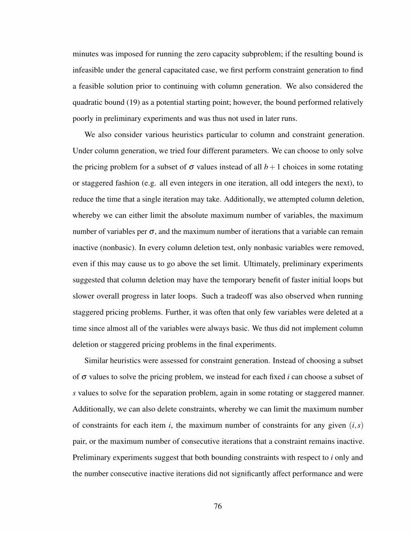
minutes was imposed for running the zero capacity subproblem; if the resulting bound is

infeasible under the general capacitated case, we first perform constraint generation to find

a feasible solution prior to continuing with column generation. We also considered the

quadratic bound (19) as a potential starting point; however, the bound performed relatively

poorly in preliminary experiments and was thus not used in later runs.

We also consider various heuristics particular to column and constraint generation.

Under column generation, we tried four different parameters. We can choose to only solve

the pricing problem for a subset of σ values instead of all b+1 choices in some rotating

or staggered fashion (e.g. all even integers in one iteration, all odd integers the next), to

reduce the time that a single iteration may take. Additionally, we attempted column deletion,

whereby we can either limit the absolute maximum number of variables, the maximum

number of variables per σ , and the maximum number of iterations that a variable can remain

inactive (nonbasic). In every column deletion test, only nonbasic variables were removed,

even if this may cause us to go above the set limit. Ultimately, preliminary experiments

suggested that column deletion may have the temporary benefit of faster initial loops but

slower overall progress in later loops. Such a tradeoff was also observed when running

staggered pricing problems. Further, it was often that only few variables were deleted at a

time since almost all of the variables were always basic. We thus did not implement column

deletion or staggered pricing problems in the final experiments.

Similar heuristics were assessed for constraint generation. Instead of choosing a subset

of σ values to solve the pricing problem, we instead for each fixed i can choose a subset of

s values to solve for the separation problem, again in some rotating or staggered manner.

Additionally, we can also delete constraints, whereby we can limit the maximum number

of constraints for each item i, the maximum number of constraints for any given (i,s)

pair, or the maximum number of consecutive iterations that a constraint remains inactive.

Preliminary experiments suggest that both bounding constraints with respect to i only and

the number consecutive inactive iterations did not significantly affect performance and were

76

thus not included in later experiments. On the contrary, bounding the number of constraints

for each (i,s) pair seemed to improve overall performance by preventing an intermediate

solve from taking too long; we thus implemented a bound of anywhere between 50 and 75

depending on the instance.

Lastly, we record the various numerical tolerances involved. The primal numerical

tolerance ε = 0.1% was used as the optimality gap threshold. The dual numerical tolerance

δ = 0.01% was used to determine whether or not a constraint is violated when determining

feasibility under constraint generation. Finally, a 0.1% threshold was used when performing

the pricing problem to determine whether a prospective variable should enter the value

function approximation.

5.3.2 Discussion

Tables D, 7, and D provide summary results for the 10, 20, and 30 item experiments,

respectively. For all tables, the initial and final gaps refer to the geometric mean of the gaps

across all instances of a particular distribution; thus, the closer the number is to 0%, the

better the bound. The relative remaining gap (RRG) refers to how much of the initial gap

was closed over the course of the algorithm (for example, if we start with an initial gap of

50% and end with a final gap of 20%, the relative remaining gap is 40%). Recall that all

10 item instances were run under a 10 hour time limit and .1% optimality gap threshold,

stopping whenever either was reached. Accordingly in table D, then, the success rate is

defined as the percentage of instances that reached the optimality gap within the time limit,

while run time is the average run time in hours for the successful instances. The incomplete

remaining gap refers to the geometric mean of the remaining gap of any instance that did

not reach the target optimality gap within the time limit.

We observe from table D that distributions D8 and D9, the two distributions that do not

have support for 0, have the highest success rate. Other distributions seem to have a lower

success rate as the variance of the distribution decreases; these results suggest that both

77

including 0 in the support and smoothing the distribution can make closing the final gap

of less than 0.5% difficult. We also observed that uncorrelated instances tend to take less

time to complete than correlated instances, which makes sense as correlated item sizes and

profits tend to make for a more difficult knapsack problem even in the deterministic case.

Full data can be found in the Appendix.

On the other hand, every 20 and 30 item instance ran Algorithm 1 for 16 ”master” loops,

regardless of time limit, to provide for a more fair comparison and to compensate for the

hardware differences due to parallelization. As such, instead of run time, we provide the

”Average Primal Loops” metric, which is the average number of constraint generation loops

needed for a given master loops of the algorithm; this is an alternate way to compare the

instance difficulty across distributions. From tables 7 and D, the average primal loops do not

seem to have a clear correlation with the relative remaining gap. Instead, generally speaking,

we observe that higher variance item size distributions correlate with a smaller relative

remaining gap. In fact, we see that D6 and D7 have their initial gaps being cut by more than

half, while D3 and D5 see an improvement of at least a 25% relative gap decrease. Intuitively

speaking, these high variance distributions are the most different from the deterministic

counterpart. Thus, our algorithm seems to work well for instances that most deviate from

the deterministic case, where perhaps a less complex algorithm or heuristic may suffice.

Recall that the 30 item instances do not have an optimal solution to benchmark against

and must run the corresponding policy for each tentative value function approximation

after every master loop. Hence, the ”bound gap closed” and ”policy gap closed” columns

in table D refer to the relative gap closed when we only observe the progress made via

the bounds and policies, respectively (i.e. the higher the percentage, the more progress

made). Similarly with the 20 item instances, there does not seem to be a strong relationship

between the average primal loops and the distribution, although a larger number of primal

loops roughly corresponds to a smaller relative remaining gap. What is most interesting

about table D is that the correlated instances see significantly better improvement than the

78

Table 6: 10 Items SummaryDist Initial Gap Final Gap RRG Success Rate Run Time (hr) Incomplete Rem.Gap

d1 13.81% 0.49% 3.67% 40% 2.3 0.76%d3 8.07% 0.21% 2.58% 40% 2.2 0.31%d5 12.73% 0.48% 3.14% 60% 2.2 1.12%d6 14.84% 0.36% 1.82% 70% 4.7 1.06%d7 16.42% 0.30% 1.54% 80% 3.5 1.32%d8 6.12% 0.02% 0.48% 100% 2.5 -d9 5.05% 0.07% 1.69% 90% 2.5 0.60%

Table 7: 20 Items SummaryDist Initial Gap Final Gap RRG Avg. Primal Loops

d1 7.83% 6.27% 81.79% 19.79d3 5.12% 3.64% 71.99% 22.84d5 13.93% 8.80% 61.48% 27.86d6 19.51% 7.78% 31.28% 21.83d7 19.53% 9.63% 38.01% 19.12d8 3.31% 2.18% 65.44% 18.18d9 2.81% 2.15% 76.21% 24.00

uncorrelated instances, and that the majority of the improvement comes from the policy side

(a 40-50% policy gap closed, compared to 0-1% policy gap closed). As correlated instances

deterministically have their size and value aligned in some way, they are more likely to have

items with similar value-to-size ratios. This makes it more difficult for our natural greedy

policies to discriminate between items to insert for a given state and can perform rather

poorly. Thus, our algorithm has the ability to provide significantly better policies when the

natural policies are insufficient. On the other hand, the uncorrelated instances generally do

see a better improvement from the bound side; aside from D5, where the bound gap closed

is roughly similar between the two instance types, the uncorrelated bound gap closed is

strictly better. All in all, our algorithm is able to improve the gap in the areas that need it the

most, depending on the whether the initial bound or initial policy is more lacking.

To help narrow down the types of instances that allow for better progress via Algorithm 1,

Figures 2 through 7 examine various parameters against the relative remaining gap, our main

79

Table 8: 30 Item SummaryType Dist Initial Gap Final Gap RRG Bnd. GapClosed Pol. GapClosed AvgPrimalLoopsCor d1 13.45% 7.30% 58.06% 2.28% 39.89% 6.16

d3 4.53% 4.42% 97.31% 2.69% 0.00% -d5 23.37% 11.14% 52.89% 3.57% 43.59% 9.29d6 34.84% 14.56% 51.25% 4.52% 45.00% 9.87d7 48.34% 17.62% 46.98% 3.27% 49.70% 15.10d8 3.52% 3.38% 95.25% 4.75% 0.00% 14.03d9 3.18% 2.91% 92.50% 2.23% 5.38% 16.22

Uncor d1 9.29% 9.00% 97.04% 2.66% 0.29% 11.22d3 3.61% 3.29% 90.79% 8.69% 0.56% -d5 13.07% 12.45% 95.40% 4.60% 0.00% 12.29d6 20.85% 18.23% 88.14% 11.86% 0.00% 7.56d7 25.02% 21.06% 84.73% 15.27% 0.00% 25.48d8 3.06% 2.47% 83.80% 8.05% 8.87% 10.57d9 2.39% 2.23% 92.55% 3.46% 4.00% 9.68

Figure 2: 20 Items - Distribution Variance vs. Relative Remaining Gap

80

Figure 3: 20 Items - Fill Rate vs. Relative Remaining Gap

Figure 4: 20 Items - Initial Gap vs. Relative Remaining Gap

81

Figure 5: 30 Items - Distribution Variance vs. Relative Remaining Gap

Figure 6: 30 Items - Fill Rate vs. Relative Remaining Gap

82

Figure 7: 30 Items - Initial Gap vs. Relative Remaining Gap

metric for progress. These plots suggest that higher fill rates, higher distribution variance,

and a higher initial gap are all positively correlated with a lower relative remaining gap.

Regarding fill rate, higher fill rates imply that an individual item will have a greater impact

on the solution. Intuitively, then, the problem is less complex in that fewer item insertions

on expectation are needed to fill the knapsack; this is reflected in the algorithm observing

greater progress per master loop. The same intuition applies to the distribution variance, as

the higher the variance of each item size, the greater the impact of an individual item has.

Additionaly, these extreme distributions also tend to have a higher observed starting gap.

Since our algorithm is more general-purpose, it is able to best improve the gap when there is

a greater initial gap to close, i.e. when the original bounds do not perform as well. Indeed,

such behavior is typical for most cutting plane algorithms in practice, whereby cutting the

gap becomes increasingly more difficult as we approach optimality.

Another metric used for progress is the relative remaining gap closed per loop, which

is the total relative gap closed divided by the number of master loops performed in the

83

algorithm run. This metric provides for a fairer comparison between the instances that were

unable to complete the specified 16 loop limit. We also compared and plotted the fill rates,

distribution variance, and initial gap to this second metric, but the results are very similar

and thus omitted here. For these additional plots, please refer to the Appendix.

Figures 8 through 11 record the distributions of the set sizes |U | of all generated wU,σ

variables at the end of the algorithm. Recalling that the 10 item instances actually solve

to (numerical) optimality, figures 8 and 9 provide insight into which set cardinalities are

more prevalent in the optimal solution. In particular, we observe a noticeable difference

in the set size distributions between the Bernoulli instances (D1, D5, D6, D7) and non-

Bernoulli instances (D3, D8, D9). The plot for Bernoulli instances is more skewed right

and has a mode of two items, which further explains why the Quadratic bound (19) (which

included both singleton and paired item sets) was the best performing approximation in

earlier experiments for these instance types. However, the plot for non-Bernoulli instances

seems to become more normally distributed as the instance’s variance decreases: D3 is

centered around set sizes of 3 and 4, D8 centered around set sizes 4 and 5, and D9 centered

around set size 5. This suggests that, at optimality, less extreme instances favor variables that

correspond to larger item set sizes since individual items have a relatively smaller impact, as

opposed to the more extreme Bernoulli instances since.

The set sizes for 20 and 30 item instances did not exhibit a noticeable difference

between the Bernoulli and non-Bernoulli distributions and are thus each presented as a

single summary plot. As these instances did not finish at optimality, their plots speak more

to the initially generated columns and can provide some insight into better starting bounds.

Keeping in mind that the starting approximation already includes all singleton set variables

(which explains the disproportionately large second column in the plots), both figures seem

to portray a bimodal distribution. The modes are roughly one-sixth and two-thirds the

number of items (4 and 13 for 20 items, 5 and 20 for 30 items), although separation between

modes is more pronounced for the 30 item instances. Such behavior suggests that including

84

Figure 8: 10 Items: wU,σ Set Size Frequencies, Bernoulli

more variables of such cardinalities would make for a better starting bound. Intuitively,

given the information provided by the variables at these modes, one can ”fill in the gaps”

and approximate the incremental value to states corresponding to the intermediate set sizes;

this can be a more efficient method than beginning with variable set sizes that are uniformly

or normally distributed, for example.

Thus, Algorithm 1 provides for a systematic way to further reduce the gap arising from

otherwise efficiently solvable bounds and policies, and it can reduce the gap significantly

so depending on where the largest areas of improvement lie. In essence, our algorithm

performs well in the situations where we need it to the most; we observe the best progress

when the initial bounds and/or heuristic policies perform the most poorly. It remains a valid

alternative to the DP formulation for larger instances that still see noticeable gaps from not

only a time perspective, but from a space perspective as well; our algorithm typically never

required more than 1.5 GB of memory throughout its run, whereas the DP would require

upwards of 15 GB memory for even the smaller 20 item instances. However, the algorithm

85

Figure 9: 10 Items: wU,σ Set Size Frequencies, Non-Bernoulli

Figure 10: 20 Items: wU,σ Set Size Frequencies

86

Figure 11: 30 Items: wU,σ Set Size Frequencies

is not yet a universal solution. Further work entails narrowing down the types of instances

where it works best (such as examining different distributions), fine-tuning our heuristics

(such as smarter or more complex column generation) for faster progress, and improving

certain theoretical guarantees (such as whether the pricing problem is truly NP-complete,

and why the algorithm is not guaranteed to systematically improve from the policy side).

Finally, as we do assume integer support in our analysis, it is also of interest to explore how

we can apply a similar algorithm approach for continuous distributions.

87

CHAPTER VI

CONCLUSIONS AND FUTURE WORK

We have extensively studied a dynamic version of the knapsack problem with stochastic

item sizes originally formulated in [14, 15]. In Chapter 2 we proposed a semi-infinite,

multiple-choice linear knapsack relaxation. We have shown how both this and a stronger

pseudo-polynomial relaxation from [31] arise from different value function approximations

being imposed on the doubly-infinite LP formulation of the problem’s DP recursion. Our

theoretical analysis shows that these bounds are stronger than comparable bounds from

the literature, while our computational study indicates that the multiple-choice knapsack

relaxation is quite strong in practice and in fact becomes tighter as the number of items

increases.

We then provided further relaxation analysis on the multiple choice knapsack bound (4).

We have shown in Chapter 3 that the MCK bound is asymptotically optimal as the number

of items increases by comparing it to a natural greedy policy and, depending on various

growth rates of capacity, delineated reasonable conditions for which the result holds.

For medium-sized instances with more item-to-capacity granularity, the gap remains

a cause for concern, and in Chapter 4, we proposed a quadratic relaxation whose value

function approximation encodes interactions between item pairs. In addition to showing

that it is polynomially solvable and more efficient than the best known pseudo-polynomial

relaxation, our computational experiments indicate that the quadratic bound is at least

stronger than MCK and faster than PP, while at best comparable to or even stronger than PP

in both quality and solution time.

Lastly, we developed a finitely terminating exact algorithm in Chapter 5 that solves the

dynamic knapsack problem within numerical tolerance, under the assumption of integer

88

item sizes and capacity. The algorithm incorporates a combination of column and constraint

generation to iteratively improve a value function approximation based on a reformulation of

the original dynamic program. We provide preliminary theoretical results that solve the zero

capacity case in full from both the bound and policy sides, as well as examine the hardness of

subproblems encountered in the more general capacitated case. An extensive computational

study points to the types of instances that see the greatest relative improvement. In particular,

the algorithm significantly closes the gap from the policy side when natural heuristic greedy

policies are lacking, while we also observe a steady gap closure from the bound side. The

bounds prescribed by the algorithm also perform particularly well when the initial gap is

relatively large.

Our results motivate additional questions. While our computational study of the quadratic

bound assumes integer support for comparison reasons, our analysis does not preclude

applying the bound to continuous distributions; it remains to examine both how to implement

the bound and its empirical performance in the continuous case. The exact algorithm

presented in the previous chapter provide theoretical guarantees from the bound side, while

the policy side can be investigated further; moreover, more complex algorithm heuristics,

such as finding a smart way to generate columns without solving an integer program, may

improve computational performance. Finally, in an even more general sense, the knapsack

problem is fundamental to the development of linear and integer programming. In a similar

vein, it would be of interest to consider whether our methods — including value function

approximations and a systematic algorithm — can be applied to other sorts of problems,

such as other combinatorial optimization problems under uncertainty.

89

APPENDIX A

FULL DATA TABLES: CHAPTER 2

The following tables present the raw data used to calculate the summary tables presented

earlier. The first five tables are used to calculate Tables 1 and 2, and they separate instances

by their size: small instances, followed by 100-item instances under continuous distributions,

100-item instances with discrete distributions, then 200-item instances under continuous

and discrete distributions. Table 11 includes running times for the PP bound and dual policy;

these are in seconds.

90

Table 9: Small instances.Instance Items Distribution PIR MCK Greedy Adapt. PP PP Dual Policy

p01 10 E 469.43 308.38 304.32 -U1 407.46 309.02 289.47 289.47U2 334.49 309.02 281.94 287.36N 347.11 308.58 284.20 287.63

p02 5 E 73.35 52.23 49.23 -U1 66.76 52.63 44.18 44.18U2 59.72 52.63 43.62 45.48N 61.42 52.52 44.63 45.20

p03 6 E 214.84 159.17 154.52 -U1 194.27 160.00 140.09 140.09U2 175.05 160.00 128.40 133.66N 177.41 159.76 132.24 133.11

p04 7 E 152.80 105.64 104.62 -U1 133.61 105.70 87.11 87.11U2 121.54 107.55 93.31 98.58N 122.19 97.76 79.26 88.35

p05 8 E 1174.89 1151.23 990.27 -U1 1155.69 1190.00 1006.87 1006.87U2 1148.92 1190.00 955.95 960.33N 1157.76 1187.67 976.79 976.39

p06 7 E 2878.60 1785.59 1687.88 -U1 2541.71 1786.50 1633.31 1633.31U2 2162.80 1786.50 1506.54 1524.70N 2211.48 1783.92 1522.41 1534.91

p07 15 E 2260.73 1461.48 1476.47 -U1 1980.37 1461.50 1390.88 1390.88U2 1748.72 1461.50 1364.71 1388.83N 1784.32 1459.35 1391.59 1409.44

p08 24 E 20824162.16 13580702.9 13373492.25 -U1 18268194.11 13580982.52 13220859.93 12445090.33U2 15901300.28 13580982.52 12868614.76 12674256.09N 16185888.15 13560987.98 12987982.5 13169542.03

p01 10 D1 487.98 394.52 296.54 321.36 385.83 315.38D2 429.27 352.02 300.94 308.37 346.27 307.38D3 424.15 337.77 296.20 307.71 327.87 304.54D4 488.86 345.97 301.53 313.49 334.23 314.79

p02 5 D1 70.11 71.00 53.99 54.81 62.50 53.92D2 64.71 61.67 45.31 45.67 55.83 46.22D3 67.89 58.33 47.95 49.75 54.86 49.74D4 75.99 67.91 50.75 50.47 58.21 53.45

p03 6 D1 206.03 209.19 148.98 148.48 169.00 153.17D2 192.01 184.71 144.33 158.80 175.67 133.81D3 198.74 176.61 135.08 147.73 164.14 149.32D4 221.40 199.33 155.59 156.67 168.61 157.56

p04 7 D1 140.36 141.79 87.50 99.88 140.75 108.98D2 130.39 126.75 103.99 108.92 124.00 109.42D3 138.11 116.86 94.75 99.35 114.35 105.32D4 153.35 137.56 104.78 107.78 125.83 109.59

p05 8 D1 1127.91 1239.78 918.26 921.34 1173.00 960.58D2 1155.83 1219.85 991.35 996.10 1111.33 1033.15D3 1141.79 1211.56 941.37 946.18 1133.81 979.05D4 1176.03 1129.89 962.53 966.43 1107.36 918.70

p06 7 D1 2751.88 2380.82 1475.97 1560.94 1922.25 1633.93D2 2449.14 2087.00 1772.02 1776.13 1988.67 1852.03D3 2544.08 1987.17 1540.79 1618.81 1881.90 1809.05D4 3007.52 2306.09 1637.78 1796.06 1935.71 1820.33

p07 15 D1 2137.13 1681.26 1490.73 1546.55 1680.75 1607.05D2 1933.20 1570.45 1461.14 1529.57 1570.45 1498.95D3 2039.99 1533.54 1389.58 1450.84 1516.37 1461.44D4 2304.04 1676.91 1439.27 1486.18 1554.73 1479.13

p08 24 D1 19515886.11 15394878.96 13258193.23 13743118.4D2 17610353.34 14477273.59 12898295.79 13541522.45D3 18882530.81 14177463.69 12996088.67 13455440.77D4 21458854.89 15281861 13429274.26 13937656.95

91

Table 10: 100 items, continuous distributions.Instance Distribution PIR MCK Greedy Adapt.100cor1 E 46802.50 30013.29 30027.84 -

U1 40845.14 30013.29 29709.86 29709.86U2 35482.96 30013.29 29659.10 29681.43N 36040.95 29969.35 29660.14 29737.86

100cor2 E 46073.75 35516.98 35523.63 -U1 40917.92 35516.98 35067.72 35067.72U2 37030.99 35516.98 35079.05 35343.20N 37466.24 35466.19 35003.46 35283.59

100cor3 E 82190.42 40886.27 40457.22 -U1 68049.76 40886.27 40482.44 40482.44U2 52659.17 40886.27 40114.07 40172.81N 53911.04 40826.58 40237.92 40279.47

100cor4 E 106258.17 44168.09 43572.86 -U1 85060.89 44168.09 43708.70 43708.70U2 58990.90 44168.09 43492.66 43533.25N 61759.77 44103.54 43352.43 43413.47

100cor5 E 60004.28 27106.08 27231.81 -U1 48705.49 27106.08 26657.77 26657.77U2 35705.48 27106.08 26655.80 26632.95N 36991.38 27066.39 26783.05 26793.98

100cor6 E 8286.74 4480.44 4511.49 -U1 6950.51 4480.44 4437.71 4437.42U2 5584.03 4480.44 4423.21 4424.94N 5688.12 4473.89 4427.14 4431.23

100cor7 E 52356.63 32128.94 32370.66 -U1 44970.77 32128.94 31593.64 31593.64U2 38720.08 32128.94 31748.74 31767.77N 39044.63 32081.98 31742.67 31752.78

100cor8 E 65439.41 31608.91 31946.24 -U1 53157.53 31608.91 31073.76 31073.76U2 40607.08 31608.91 31068.39 31091.21N 41831.26 31562.71 31173.94 31230.02

100cor9 E 31530.91 16491.00 16307.28 -U1 26472.68 16491.00 16361.04 16361.04U2 20837.16 16491.00 16225.89 16232.88N 21330.34 16466.92 16300.77 16294.04

100cor10 E 123118.83 73558.26 73383.78 -U1 105636.61 73558.26 72754.22 72754.22U2 89404.56 73558.26 72482.59 72528.14N 90931.11 73450.59 72719.15 72628.02

100uncor1 E 42769.68 38457.56 38229.38 -U1 40682.51 38457.56 38215.75 38215.75U2 39083.20 38457.56 38169.62 38265.87N 39292.73 38403.27 38188.09 38264.49

100uncor2 E 18129.49 15212.48 15190.47 -U1 16632.99 15212.48 15044.51 15044.51U2 15659.71 15212.48 15065.95 15141.41N 15775.43 15190.87 15021.03 15096.71

100uncor3 E 80130.74 65503.10 64733.69 -U1 73939.67 65503.10 65055.60 65055.60U2 67715.12 65503.10 64584.03 64862.53N 68481.73 65410.69 64863.15 65078.84

100uncor4 E 111922.24 85139.17 83845.66 -U1 99104.63 85139.17 84369.32 84369.32U2 87870.48 85139.17 83987.41 84559.16N 89266.56 85018.36 83877.86 84406.85

100uncor5 E 57965.38 44361.56 44315.31 -U1 51796.03 44361.56 43716.36 43716.36U2 46325.52 44361.56 43694.02 43905.13N 47050.67 44298.81 43843.21 43954.99

100uncor6 E 8308.34 6950.75 6962.80 -U1 7687.99 6950.75 6880.37 6880.37U2 7178.39 6950.75 6888.15 6922.83N 7227.76 6940.92 6896.62 6919.74

100uncor7 E 48193.33 42746.90 42627.88 -U1 45494.95 42746.90 42424.58 42424.58U2 43814.00 42746.90 42468.59 42618.12N 43900.48 42686.66 42393.66 42532.98

100uncor8 E 63238.76 49921.48 50080.69 -U1 57161.84 49921.48 49358.21 49358.21U2 51907.49 49921.48 49312.42 49470.25N 52639.12 49851.04 49375.43 49533.99

100uncor9 E 32346.23 25826.46 25474.05 -U1 29550.41 25826.46 25574.67 25574.67U2 26956.78 25826.46 25524.10 25636.02N 27341.30 25789.76 25554.41 25629.55

100uncor10 E 112928.12 100349.64 99560.75 -U1 106740.87 100349.64 99709.53 99709.53U2 102073.99 100349.64 99555.19 99906.87N 102725.17 100208.51 99653.15 99945.11

92

Table 11: 100 items, discrete distributions.Instance Distribution PIR MCK Greedy Adapt. PP PP Time PP Dual Policy PP Policy Time100cor1 D1 44078.58 31111.79 29798.00 30087.17

D2 39734.36 30562.79 29844.35 30126.53D3 42432.33 30379.70 29681.42 29938.09D4 48581.92 30995.20 29860.49 30225.65

100cor2 D1 46747.43 36615.48 35463.69 35761.03 36615.48 4151.59 35190.17 3549.92D2 42845.17 36066.48 35075.34 35383.89 36044.08 16575.69 34503.27 7204.37D3 42835.04 35883.40 35327.66 35553.73 35880.92 7822.71 35464.01 4142.33D4 47111.17 36462.66 34935.83 35019.59 36036.74 45026.36 34800.01 8278.49

100cor3 D1 82283.49 43071.27 40846.87 41608.34D2 68298.72 41981.27 40383.90 40443.97D3 69105.73 41617.11 40587.21 41198.20D4 86687.28 42707.30 41218.08 42104.89

100cor4 D1 117391.61 47466.59 44318.90 45797.99D2 93455.42 45817.59 43831.99 44884.43D3 89015.11 45267.84 43611.86 44516.14D4 111984.10 46307.87 43515.92 44274.00

100cor5 D1 62714.78 28754.58 27524.52 28089.91D2 50514.96 27930.58 26841.43 27175.15D3 49465.22 27655.83 26871.22 27313.78D4 63768.18 28303.23 27625.25 28137.76

100cor6 D1 8111.63 4699.44 4558.40 4674.98 4699.44 5958.01 4601.82 4599.36D2 6913.01 4590.11 4472.36 4517.99 4586.17 17836.77 4519.63 8730.71D3 7107.33 4553.61 4458.65 4522.50 4553.00 8430.32 4509.02 4298.07D4 8712.30 4648.74 4406.69 4477.31 4576.45 55665.90 4534.99 9986.10

100cor7 D1 49546.25 33436.44 32141.17 32363.01D2 43752.40 32784.77 31609.47 31799.30D3 46749.00 32566.85 32075.44 32424.55D4 54808.02 33217.02 32228.47 32478.68

100cor8 D1 66226.71 33454.41 31511.43 32404.03D2 54942.13 32531.91 31544.68 32034.34D3 54220.66 32224.33 31233.43 31740.84D4 68773.82 32946.54 31735.01 32129.03

100cor9 D1 31232.40 17358.50 16382.66 16817.33 17358.50 5850.62 16788.91 4575.07D2 26594.32 16926.83 16348.04 16568.27 16912.50 19652.41 16597.11 10150.56D3 26885.93 16782.25 16148.36 16358.36 16780.97 9340.53 16552.22 4361.77D4 33311.77 17173.90 16304.31 16506.94 16870.03 54863.39 16309.74 10862.59

100cor10 D1 117896.42 76476.76 72575.76 73691.05 76476.76 7638.23 75054.18 4311.85D2 103974.56 75021.92 73437.07 74136.90 74956.18 21293.51 74189.98 6974.64D3 109504.05 74535.51 73005.68 73711.17 74529.54 8805.79 74141.82 5041.93D4 130641.57 76078.30 73419.19 74356.02 74893.66 60621.26 74349.03 12521.45

100uncor1 D1 43115.77 39050.18 38114.19 38283.15 39050.18 4907.27 37556.94 4432.39D2 41689.79 38758.85 38322.44 38544.31 38740.96 23577.82 38063.65 8963.41D3 41423.69 38661.78 38133.94 38303.53 38660.16 8333.15 37402.40 4266.99D4 43230.58 39021.74 38229.45 38327.39 38758.69 42589.05 37639.14 11467.26

100uncor2 D1 18305.73 15608.14 15128.88 15271.97D2 17234.28 15412.16 15037.50 15179.70D3 17291.71 15346.20 15077.58 15154.24D4 18427.78 15539.47 14963.46 15052.44

100uncor3 D1 83194.39 67360.00 64770.18 65599.72D2 77194.25 66434.19 64582.40 65345.69D3 76370.51 66125.42 65102.31 65632.90D4 82585.46 67221.26 65343.83 65601.12

100uncor4 D1 123509.36 88088.17 84788.51 85715.22 88088.17 4986.33 83504.80 2777.83D2 111075.84 86618.00 84761.74 85598.76 86571.83 18304.86 84222.73 6596.08D3 107340.42 86126.50 84122.96 84848.73 86119.50 7340.91 84475.59 3149.88D4 116383.28 87154.15 84122.40 84715.31 86505.92 53716.99 83185.47 7839.50

100uncor5 D1 61386.43 45854.42 44556.04 45051.44D2 55698.81 45108.73 43922.13 44418.12D3 54356.52 44859.89 43913.47 44198.48D4 60245.42 45503.07 44623.99 44901.59

100uncor6 D1 8480.72 7102.63 6970.49 7033.13 7102.63 4392.03 6619.18 3341.61D2 8013.10 7025.64 6939.90 6989.11 7022.13 15157.58 6833.16 6890.15D3 7950.84 7000.58 6869.04 6912.14 7000.25 7619.60 6825.17 3696.61D4 8471.81 7093.54 6862.53 6889.23 7025.20 46301.52 6805.25 9100.62

100uncor7 D1 48576.04 43527.70 42340.84 42708.69D2 46607.41 43144.45 42394.98 42700.89D3 46716.27 43014.32 42643.76 42797.71D4 48788.27 43459.26 42720.55 42862.96

100uncor8 D1 65960.71 51435.98 49780.27 50388.94D2 60674.89 50681.48 49548.72 50231.46D3 59922.36 50429.06 49508.31 49961.63D4 65312.69 51143.14 49988.34 50285.08

100uncor9 D1 33455.01 26586.96 25502.40 25833.05D2 31068.63 26209.79 25697.86 25913.22D3 30813.52 26083.04 25441.93 25611.47D4 33430.11 26438.54 25421.77 25612.58

100uncor10 D1 114587.82 102187.14 99022.08 99565.20 102187.14 4442.64 98938.86 3804.11D2 109941.05 101282.97 99847.93 100505.43 101238.42 16119.72 99264.64 8712.19D3 109400.87 100976.72 99540.08 99943.73 100970.68 7832.96 99153.42 4192.16D4 114394.12 101825.76 99687.04 100010.95 101181.44 52132.86 98602.11 9252.24

93

Table 12: 200 items, continuous distributions.Instance Distribution PIR MCK Greedy Adapt.200cor1 E 96338.10 60298.25 60166.15 -

U1 83447.70 60298.25 59870.89 59883.76U2 72345.57 60298.25 59880.24 59982.77N 73305.69 60209.82 59989.26 60092.64

200cor2 E 42804.74 24268.53 24315.10 -U1 36386.10 24268.53 24231.19 24227.91U2 29961.30 24268.53 24105.67 24113.98N 30382.63 24233.01 24061.61 24086.15

200cor3 E 160487.58 79385.20 79848.79 -U1 133231.17 79385.20 79010.52 79010.52U2 102274.99 79385.20 78698.19 78727.61N 104766.79 79269.21 78849.13 78924.35

200cor4 E 242915.02 119112.85 119238.33 -U1 199950.22 119112.85 118310.85 118310.85U2 153931.66 119112.85 118062.12 118110.00N 157688.69 118938.55 118463.94 118742.97

200cor5 E 111488.65 50763.78 51076.94 -U1 91264.23 50763.78 50779.10 50779.10U2 66731.70 50763.78 50318.23 50351.14N 68941.15 50689.58 50432.74 50456.02

200cor6 E 17065.10 8985.94 9015.47 -U1 14304.83 8985.94 8969.54 8970.44U2 11411.90 8985.94 8921.87 8928.95N 11600.03 8972.78 8917.48 8922.45

200cor7 E 108614.77 65325.84 65922.25 -U1 93490.58 65325.84 65118.22 65118.22U2 79269.30 65325.84 64920.35 65033.72N 80272.94 65230.19 64790.51 64889.80

200cor8 E 130055.50 62201.63 61390.91 -U1 107213.96 62201.63 62183.34 62183.34U2 80820.28 62201.63 61582.15 61695.99N 83030.03 62110.58 61730.68 61774.10

200cor9 E 66615.12 33899.19 33749.25 -U1 55341.71 33899.19 33601.75 33602.05U2 43378.55 33899.19 33643.96 33662.58N 44269.81 33849.60 33606.65 33643.12

200cor10 E 242014.96 140855.75 140610.79 -U1 205686.65 140855.75 139359.83 139359.83U2 173062.12 140855.75 139596.58 139810.62N 175291.42 140649.33 139763.01 139782.13

200uncor1 E 83826.87 74467.00 74034.84 -U1 79249.11 74467.00 74121.03 74121.03U2 75919.43 74467.00 74199.79 74365.84N 76324.76 74361.68 74229.32 74400.45

200uncor2 E 38095.74 32017.00 31838.94 -U1 35427.90 32017.00 32013.82 32013.20U2 32959.84 32017.00 31838.69 31929.72N 33285.84 31971.64 31895.73 31954.88

200uncor3 E 151605.79 121926.52 121991.71 -U1 139020.13 121926.52 121820.38 121820.38U2 126906.94 121926.52 121218.31 121640.45N 128281.47 121754.37 121467.90 121860.33

200uncor4 E 216014.95 163613.50 163269.93 -U1 192158.61 163613.50 163316.27 163316.27U2 168956.10 163613.50 162434.29 162972.92N 171875.64 163381.50 162524.27 163109.14

200uncor5 E 116500.76 89506.64 89658.43 -U1 104709.27 89506.64 89233.56 89233.56U2 93160.65 89506.64 88888.94 89256.67N 94495.16 89379.97 89040.21 89285.07

200uncor6 E 16061.66 13183.89 13124.95 -U1 14799.72 13183.89 13154.57 13154.57U2 13638.73 13183.89 13118.35 13171.13N 13775.38 13165.22 13103.32 13136.81

200uncor7 E 98162.02 85512.00 85730.66 -U1 92160.36 85512.00 85344.42 85342.96U2 87635.96 85512.00 85047.56 85279.20N 88124.33 85391.03 85111.43 85337.96

200uncor8 E 126731.98 99398.79 98822.78 -U1 114892.19 99398.79 99214.48 99214.48U2 103848.29 99398.79 98714.26 99114.09N 105151.92 99257.96 98803.43 99135.01

200uncor9 E 63113.62 52263.71 52039.60 -U1 58289.71 52263.71 51949.95 51949.95U2 54032.26 52263.71 51990.51 52107.29N 54479.66 52189.96 51920.80 52035.21

200uncor10 E 228662.27 200005.23 199130.12 -U1 215045.49 200005.23 198547.30 198547.30U2 204372.46 200005.23 199040.80 199532.21N 205686.78 199722.65 199202.04 199547.32

94

Table 13: 200 items, discrete distributions.Instance Distribution PIR MCK Greedy Adapt.200cor1 D1 90688.56 61396.75 60471.88 61118.87

D2 80392.29 60847.75 59973.48 60394.04D3 87585.08 60664.67 60080.24 60431.39D4 100236.02 61343.83 60229.68 60489.84

200cor2 D1 41009.55 24817.03 24410.57 24597.46D2 35477.81 24543.03 24236.69 24360.78D3 37442.18 24451.62 24311.92 24428.50D4 45364.72 24744.38 24288.52 24522.92

200cor3 D1 162086.31 81570.20 80423.03 81219.60D2 133748.93 80480.20 79151.98 79762.27D3 134781.28 80116.03 79464.88 80077.16D4 169279.67 81258.86 79164.22 79743.83

200cor4 D1 242362.08 122411.35 118933.94 120813.60D2 202178.61 120762.35 119490.55 120327.60D3 202501.13 120212.60 118489.64 119214.81D4 257291.96 121803.45 120456.40 121202.45

200cor5 D1 116224.49 52412.28 50387.32 50994.89D2 93695.69 51588.28 50121.57 50583.33D3 92933.34 51313.53 50891.46 51311.03D4 118255.65 52009.95 50748.44 51528.33

200cor6 D1 16667.82 9205.94 9003.34 9106.95D2 14088.38 9095.94 8907.81 8968.55D3 14567.33 9059.27 8941.13 9011.57D4 18095.95 9178.19 8952.46 8994.52

200cor7 D1 102607.10 66642.84 64916.83 65453.53D2 90080.82 65984.84 64946.43 65266.42D3 96574.97 65765.34 64822.58 65276.06D4 114182.03 66524.37 65017.83 65403.32

200cor8 D1 132461.57 64047.13 62223.70 63217.74D2 108756.60 63124.63 61399.19 61918.21D3 108834.42 62817.05 61893.55 62310.26D4 137941.23 63603.00 61671.69 62269.95

200cor9 D1 66481.90 34778.19 33987.45 34397.40D2 55414.74 34338.86 33860.73 34054.50D3 56553.93 34192.36 33772.89 34057.41D4 70323.25 34657.10 33988.19 34193.42

200cor10 D1 229580.17 143794.25 141221.53 142346.43D2 201176.03 142326.08 140948.56 141848.39D3 212590.51 141836.33 139834.33 140638.72D4 255690.49 143493.23 140397.94 141323.06

200uncor1 D1 84447.87 75162.20 74102.30 74307.92D2 81096.68 74813.83 74230.71 74522.35D3 81238.31 74700.25 74330.17 74590.06D4 84706.40 75093.47 74297.73 74582.78

200uncor2 D1 38811.55 32417.83 32048.10 32157.17D2 36597.59 32219.29 31917.73 32063.47D3 36613.97 32152.18 31985.14 32093.07D4 38989.23 32374.63 31867.19 31942.49

200uncor3 D1 158094.32 123827.63 122889.66 123655.48D2 145651.06 122875.33 121582.47 122542.66D3 144406.92 122558.61 121787.37 122154.81D4 156247.13 123656.16 121416.58 121944.74

200uncor4 D1 238200.06 166562.50 163103.08 163965.87D2 213766.66 165092.33 163313.96 164468.05D3 205287.22 164600.83 162319.57 162955.55D4 225416.49 166012.44 163373.89 164113.67

200uncor5 D1 123852.35 90999.64 89043.21 89447.13D2 112132.05 90253.81 88750.38 89442.92D3 110653.75 90004.98 89358.15 89756.49D4 120673.15 90768.88 89096.84 89682.88

200uncor6 D1 16517.84 13364.33 13183.64 13256.00D2 15352.69 13274.02 13092.94 13171.47D3 15329.02 13244.44 13167.72 13218.32D4 16503.13 13349.34 13146.05 13179.44

200uncor7 D1 98688.98 86349.50 85006.35 85282.14D2 94372.49 85930.83 84892.45 85265.85D3 94534.69 85791.25 85087.12 85288.38D4 99266.65 86283.90 84831.98 84951.58

200uncor8 D1 132038.75 101076.29 99315.64 100116.67D2 121102.25 100237.79 98209.04 98988.87D3 120143.78 99958.20 98840.34 99262.39D4 131384.51 100801.51 98603.26 98916.01

200uncor9 D1 65358.21 52999.90 52366.24 52726.75D2 61017.13 52632.55 52057.64 52412.13D3 60666.27 52509.96 52029.22 52215.54D4 64814.11 52888.59 52202.51 52374.32

200uncor10 D1 231720.24 202053.73 199875.06 200492.32D2 221326.69 201050.06 199941.10 200897.58D3 220687.45 200708.65 198916.38 199506.77D4 232013.10 201812.81 199357.95 199830.64

95

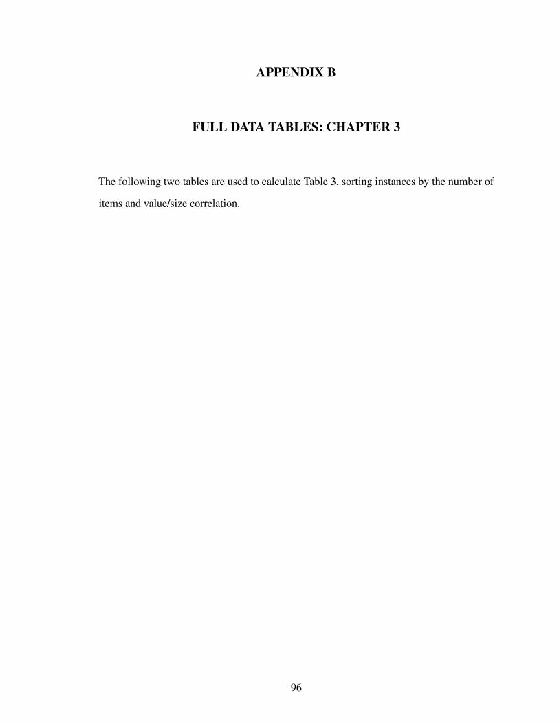
APPENDIX B


The following two tables are used to calculate Table 3, sorting instances by the number of

items and value/size correlation.

96

Table 14: MCK Data, Power Law Distribution, 200-items or LessInstance MCK Greedy A. Greedy

p01 369.34 349.82 348.83p02 72.87 60.82 60.82p03 212.21 180.30 180.30p04 146.10 131.97 132.04p05 1242.17 1070.67 1070.67p06 2497.52 2191.94 2189.40p07 1897.53 1744.87 1738.67p08 17065398.26 15332135.32 15469247.43

20cor1 7504.33 6858.15 6783.3920cor2 8495.93 8030.01 8031.3920cor3 10371.71 9969.06 10027.8220cor4 11187.62 10131.50 10019.4920cor5 6979.69 6604.17 6669.5920cor6 1126.99 1052.35 1058.9620cor7 8103.30 7311.75 7324.9620cor8 8026.99 7312.61 7241.7120cor9 4103.90 3848.59 3924.19

20cor10 18587.37 17658.55 17929.5520uncor1 8277.87 7849.25 7849.2520uncor2 4207.25 3943.93 3944.2120uncor3 15014.30 14523.65 14526.5820uncor4 18845.34 17275.89 17275.8920uncor5 10288.87 9954.37 9960.3620uncor6 1593.90 1488.41 1487.9420uncor7 9153.27 8801.53 8801.5320uncor8 12234.28 11316.91 11324.5420uncor9 6233.18 5797.05 5787.13

20uncor10 19891.23 18375.25 18365.43100cor1 33533.65 31772.52 32318.73100cor2 38866.70 36780.04 36769.95100cor3 46368.04 43344.55 44229.84100cor4 50301.94 47388.26 47682.37100cor5 30781.90 29208.76 29034.12100cor6 5033.14 4636.62 4602.74100cor7 35922.11 33927.69 33739.77100cor8 35698.90 34233.56 34325.90100cor9 18557.13 17566.13 17708.15


100uncor10 106115.85 102988.85 102929.06200cor1 65708.55 63217.98 63556.02200cor2 26431.17 25274.80 25106.71200cor3 87008.78 82050.82 82650.50200cor4 130352.19 124587.55 124232.07200cor5 55696.15 52958.54 52867.65200cor6 9824.42 9507.29 9490.57200cor7 71119.96 66871.64 67436.64200cor8 68175.46 65067.17 65485.54200cor9 37102.22 35941.59 35904.41


200uncor10 209604.85 201695.03 201589.8097

Table 15: MCK Data, Power Law Distribution, 1000-items or MoreInstance MCK Greedy1000cor1 315264.55 307486.431000cor2 131236.29 128081.911000cor3 410934.14 400298.471000cor4 440705.41 421668.991000cor5 268217.52 260201.531000cor6 47179.25 45939.641000cor7 355539.42 344511.521000cor8 335816.69 323768.201000cor9 177072.28 171585.13

1000cor10 767191.66 740630.341000uncor1 391929.12 384251.441000uncor2 175596.93 172014.691000uncor3 621566.89 608010.991000uncor4 808590.19 783339.411000uncor5 438494.83 430533.171000uncor6 69614.53 68235.171000uncor7 455682.16 444646.371000uncor8 522609.12 509452.671000uncor9 264472.90 259231.62

1000uncor10 1036098.43 1015379.722000cor1 623983.64 612009.702000cor2 259153.22 253320.692000cor3 813604.92 797448.722000cor4 874478.26 855899.422000cor5 529873.66 516339.692000cor6 93531.02 92192.952000cor7 705421.70 693901.822000cor8 661333.70 647891.312000cor9 349850.29 342958.98

2000cor10 1519181.85 1491618.082000uncor1 793470.46 786050.412000uncor2 356405.87 350868.752000uncor3 1263783.49 1244592.102000uncor4 1588156.89 1564959.332000uncor5 887755.32 872425.952000uncor6 134925.29 133512.392000uncor7 920206.84 909101.432000uncor8 1044295.46 1028806.602000uncor9 518843.38 511672.97

2000uncor10 2029051.70 2001541.975000cor1 83408.71 82305.075000cor2 133539.89 130877.495000cor3 147936.54 145219.085000cor4 116621.03 114350.125000cor5 171416.52 168773.19

5000uncor1 186921.47 185023.045000uncor2 466960.21 458038.465000uncor3 543677.26 535866.145000uncor4 368417.42 363813.335000uncor5 688418.44 678296.3610000cor1 165868.02 163120.5210000cor2 265578.99 262597.5210000cor3 291580.75 286776.1810000cor4 230855.23 225903.0010000cor5 338955.87 332911.51

10000uncor1 369884.94 365057.4410000uncor2 915640.89 906978.2510000uncor3 1074579.51 1058598.8710000uncor4 728925.87 717570.7310000uncor5 1323898.28 1298820.65

98

APPENDIX C


The following three tables present the raw data used to calculate the summaries in Tables

4 and 5. These three tables separate instances by their size: small instances, followed by

20-item instances with correlated values-to-sizes under discrete distributions, then 20-item

instances with uncorrelated values-to-sizes under discrete distributions.

99

Table 16: Quadratic Variables Data, Small Instances.Instance Distribution MCK PP PPIR Quad PP+Quad Greedy Adapt. Greedy PP Dual Quad Dual

p01 D1 352.02 346.27 405.64 351.16 - 300.94 308.37 307.38 309.68D2 394.52 385.83 386.43 389.84 380.96 296.54 321.36 315.38 311.48D3 471.02 439.00 387.11 451.67 - 334.03 344.80 366.77 342.84D4 474.25 474.25 388.13 432.63 - 354.05 364.11 376.27 358.08D5 500.40 500.40 388.50 432.78 - 363.98 366.67 410.17 397.42D6 337.77 327.87 402.58 337.47 327.56 296.20 307.71 304.54 298.74D7 345.97 334.23 431.92 344.08 - 301.53 313.49 314.79 317.40

p02 D1 61.67 55.83 73.95 61.39 54.56 45.31 45.67 46.22 46.48D2 71.00 62.50 70.15 69.78 60.38 53.99 54.81 53.92 53.98D3 70.00 70.00 56.57 58.96 - 56.04 56.07 56.12 50.30D4 58.50 58.50 46.64 45.52 - 45.90 45.90 45.74 45.74D5 72.80 72.80 52.72 52.52 - 51.50 51.50 51.00 51.00D6 58.33 54.86 75.55 58.23 54.85 47.95 49.75 49.74 49.53D7 67.91 58.21 68.67 62.55 57.47 50.75 50.47 53.45 53.36

p03 D1 184.71 175.67 217.71 183.28 173.07 144.33 158.80 133.81 152.25D2 209.19 169.00 194.32 204.15 167.00 148.98 148.48 153.17 154.06D3 211.67 211.67 169.32 183.52 - 164.99 165.06 164.94 163.30D4 165.50 165.50 124.43 130.18 - 124.62 124.62 126.82 124.24D5 213.00 213.00 124.43 150.28 - 142.33 142.33 146.05 146.05D6 176.61 164.14 219.19 175.91 162.27 135.08 147.73 149.32 147.45D7 199.33 168.61 202.02 184.62 166.94 155.59 156.67 157.56 143.65

p04 D1 126.75 124.00 162.72 126.00 123.33 103.99 108.92 109.42 104.13D2 141.79 140.75 127.13 141.50 134.63 87.50 99.88 108.98 107.04D3 139.33 139.33 114.31 116.96 - 96.18 94.37 111.31 111.31D4 151.50 151.50 127.80 132.05 - 109.67 109.83 130.15 130.15D5 158.80 158.80 146.62 141.90 - 125.27 125.27 145.07 141.98D6 116.86 114.35 149.45 119.75 114.16 94.75 99.35 105.32 97.63D7 137.56 125.83 144.97 129.40 124.04 104.78 107.78 109.59 106.52

p05 D1 1219.85 1111.33 1338.65 1218.88 1103.56 991.35 996.10 1033.15 1028.22D2 1239.78 1173.00 1247.28 1236.01 1164.25 918.26 921.34 960.58 947.04D3 1024.67 1024.67 889.22 935.78 - 867.13 865.68 910.20 897.61D4 1095.50 1095.50 930.34 1020.50 - 959.19 960.38 1003.56 936.53D5 1054.00 1054.00 875.88 861.87 - 853.88 853.88 889.88 889.88D6 1211.56 1133.81 1278.36 1211.08 1130.10 941.37 946.18 979.05 957.61D7 1129.89 1107.36 1059.41 1209.71 1048.79 962.53 966.43 918.70 878.28

p06 D1 2087.00 1988.67 2485.53 2082.37 1985.17 1772.02 1776.13 1852.03 1792.52D2 2380.82 1922.25 2218.39 2368.12 1909.46 1475.97 1560.94 1633.93 1559.56D3 2958.48 2764.67 2393.13 2686.76 - 2084.78 2104.84 2126.95 2108.86D4 2182.00 2182.00 1860.19 1910.25 - 1701.44 1701.44 1921.41 1815.08D5 2276.00 2276.00 1732.95 1823.04 - 1808.38 1808.38 1807.50 1626.21D6 1987.17 1881.90 2689.52 1985.12 1879.91 1540.79 1618.81 1809.05 1687.37D7 2306.09 1935.71 2655.66 2193.54 1931.33 1637.78 1796.06 1820.33 1739.47

p07 D1 1570.45 1570.45 1780.77 1569.79 - 1461.14 1529.57 1498.95 1516.65D2 1681.26 1680.75 1850.65 1679.10 - 1490.73 1546.55 1607.05 1595.13D3 1904.19 1890.33 1887.40 1892.80 - 1617.39 1681.45 1662.63 1621.57D4 2122.19 2100.00 1978.83 2085.72 - 1477.46 1609.41 1722.90 1674.19D5 2332.70 2063.80 1819.78 2266.79 - 1597.48 1631.31 1604.12 1603.04D6 1533.54 1516.37 1861.40 1533.39 - 1389.58 1450.84 1461.44 1448.73D7 1676.91 1554.73 2024.00 1657.24 - 1439.27 1486.18 1479.13 1486.89

100

Table 17: Quadratic Variables Data, 20 Items, Correlated Values and Sizes.Instance Distribution MCK PP PPIR Quad Greedy A. Greedy PP Dual Quad Dual20cor1 D1 6547.70 6534.08 7482.03 6544.87 5938.42 6099.08 6171.09 6156.53

D2 7062.53 7062.53 7874.59 7043.21 5924.07 6222.89 6286.62 6328.47D3 8060.70 8006.22 8230.19 7968.06 6209.93 6622.21 6717.28 6817.85D4 9008.53 9008.53 8347.92 8797.18 6568.58 6758.89 7049.40 7079.77D5 9872.03 9805.00 8393.61 9480.92 6460.73 6682.43 7253.35 7244.89D6 6373.28 6366.73 7790.07 6372.43 5806.62 6067.55 6113.27 6025.11D7 6851.31 6488.59 6804.82 6804.82 5908.74 6249.09 6173.48 6172.98

20cor2 D1 7971.85 7961.11 8518.85 7966.16 7141.35 7308.58 6997.31 7154.89D2 8351.73 8351.73 8652.96 8325.22 7296.38 7408.28 7188.36 6916.18D3 9009.65 8974.28 8908.13 8883.68 7415.06 7594.17 7516.15 7166.26D4 9602.87 9572.50 8472.94 9310.09 7522.97 7782.96 7455.27 7218.99D5 10139.45 10116.92 8767.71 9636.28 7674.77 7879.19 7759.27 7636.61D6 7830.75 7826.85 8746.74 7827.80 7210.61 7188.83 7114.96 7120.59D7 8092.27 7912.47 9282.23 7931.27 7305.33 7308.93 7432.47 7256.60

20cor3 D1 9167.63 9149.73 11004.46 9158.33 7898.79 8146.01 8170.18 8269.54D2 10191.30 10191.30 11817.91 10141.93 8043.78 8711.34 9247.72 9155.65D3 12137.80 12055.31 12962.33 11999.00 8971.92 9594.06 10268.15 10407.83D4 13998.30 13833.00 12794.14 13722.50 9503.80 9873.56 11328.91 11303.56D5 15792.60 15588.80 12769.80 15229.32 9888.71 9768.93 12051.51 12042.22D6 8824.38 8798.57 11687.14 8821.12 7705.19 8478.39 8663.99 8476.06D7 9573.95 9022.65 13369.87 9536.87 8198.66 8534.60 8697.73 8787.18

20cor4 D1 10200.86 10179.83 13043.34 10196.21 8098.62 8666.75 9203.79 9371.50D2 11760.36 11741.71 14253.92 11726.95 8565.03 10066.95 10104.68 10369.92D3 14818.20 14437.33 13516.45 14627.58 9887.58 11047.59 12575.56 12608.51D4 16348.50 16348.50 13881.98 15889.58 10618.45 10363.27 13009.51 12166.32D5 17548.40 17548.40 15631.80 16634.45 11119.24 11104.42 14744.74 12180.50D6 9673.61 9520.03 14217.35 9672.23 8086.77 8599.69 8585.73 8756.69D7 10311.55 9854.05 14797.58 10291.88 8891.16 9659.94 9588.59 9456.18

20cor5 D1 6315.83 6303.58 7719.30 6307.18 5196.81 5633.79 5973.04 5675.84D2 7096.00 7096.00 8322.12 7051.67 5560.68 6004.09 6281.05 6164.11D3 8543.33 8445.39 8565.03 8435.97 5946.88 6651.50 6808.53 6670.57D4 9938.25 9777.25 8600.85 9693.92 6764.61 6761.31 7738.69 7691.69D5 11250.80 10944.30 9118.71 10758.67 6764.45 6492.35 8851.44 8978.54D6 6052.17 6003.79 8159.53 6049.07 5299.73 5657.62 5695.33 5454.26D7 6352.19 6138.62 9022.90 6347.28 5609.18 6062.61 6078.36 6092.79

20cor6 D1 998.89 996.92 1269.46 997.45 872.51 899.58 899.92 920.02D2 1104.06 1104.06 1269.46 1096.32 892.04 956.31 1008.61 997.88D3 1299.39 1291.50 1359.22 1277.95 939.93 1004.98 1104.02 1087.76D4 1480.81 1475.75 1359.42 1441.68 970.79 1086.13 1201.09 1172.85D5 1653.66 1621.60 1358.33 1587.92 1091.82 1070.46 1279.56 1227.35D6 963.56 961.08 1241.42 963.06 884.08 929.92 932.67 911.48D7 1034.44 980.37 1400.67 1031.17 887.65 927.52 945.48 941.73

20cor7 D1 7053.95 7039.38 7732.74 7050.94 6357.79 6577.62 6622.64 6548.44D2 7480.29 7480.29 8003.99 7463.71 6544.66 6848.10 6902.24 6947.41D3 8304.81 8247.00 8193.68 8249.22 6769.86 6823.11 6894.86 7017.23D4 9115.14 9115.14 8226.35 8909.89 7012.93 6955.11 7229.98 7150.56D5 9876.44 9876.44 8544.11 9464.60 6888.49 7026.79 7455.42 7330.65D6 6910.95 6904.42 8035.97 6909.94 6489.57 6614.30 6521.30 6607.52D7 7312.33 7017.08 8448.43 7278.05 6757.69 6835.66 6886.63 6821.70

20cor8 D1 7296.63 7282.72 8939.19 7287.19 6138.55 6690.95 6839.47 6684.11D2 8209.63 8209.63 9613.26 8152.57 6501.86 6858.07 7225.20 7317.30D3 9977.80 9742.28 9519.25 9748.99 6634.92 7654.29 8558.24 8443.90D4 11544.38 11439.69 10196.18 11166.77 8063.33 7958.40 9802.36 9725.50D5 13056.73 12622.10 10686.75 12305.75 7957.51 7720.70 10160.77 9836.96D6 6991.55 6889.97 9417.43 6988.52 6088.47 6326.56 6404.30 6275.00D7 7343.18 7080.65 10206.42 7329.18 6322.24 6924.74 6827.74 6853.21

20cor9 D1 3643.67 3636.42 4382.46 3640.93 3092.34 3210.85 3225.14 3276.31D2 4050.00 4050.00 4710.08 4031.84 3291.87 3592.65 3537.75 3545.01D3 4846.00 4809.83 5204.72 4760.54 3491.23 3687.15 4041.59 4174.19D4 5574.25 5509.25 5024.08 5423.81 3753.73 4153.73 4577.26 4582.35D5 6272.00 6155.50 5176.30 5999.72 3679.98 3715.32 4937.54 4740.97D6 3507.33 3502.72 4621.36 3506.50 3121.35 3298.69 3296.45 3266.92D7 3776.45 3568.20 5252.18 3759.85 3263.37 3505.23 3573.86 3537.96

20cor10 D1 16391.77 16359.07 18868.03 16379.27 14302.77 14553.03 15176.72 15114.48D2 17818.10 17818.10 19839.74 17750.67 15328.02 15732.37 16010.08 16136.21D3 20555.60 20424.80 20613.51 20352.69 15226.99 15847.02 16770.37 17089.64D4 23124.60 23060.00 22326.61 22695.50 17066.65 16519.04 18556.25 18563.54D5 25642.00 25230.50 21020.76 23979.03 17100.77 17696.29 19030.89 19249.09D6 15914.68 15832.62 19805.42 15910.38 14330.15 14779.72 15087.60 14951.00D7 17151.96 16228.57 21888.46 17057.42 15066.57 15724.06 15785.30 15973.79

101

Table 18: Quadratic Variables Data, 20 Items, Uncorrelated Values and Sizes.Instance Distribution MCK PP PPIR Quad Greedy A. Greedy PP Dual Quad Dual20uncor1 D1 8040.61 8034.14 8106.02 8023.93 7676.97 7772.54 7109.04 7244.76

D2 8219.74 8219.74 8294.37 8183.20 7688.70 7736.41 7144.15 7033.34D3 8521.33 8502.00 8261.00 8407.86 7645.62 7692.22 6610.58 6993.62D4 8765.09 8765.09 7834.22 8554.09 7743.69 7770.24 6807.32 7056.08D5 8907.79 8904.30 8250.04 8664.80 7665.39 7686.12 6588.37 7045.17D6 7969.78 7967.45 8250.04 7961.69 7666.59 7731.04 7485.29 7293.07D7 8068.13 8014.39 8560.95 8019.48 7590.91 7647.48 7524.03 7430.56

20uncor2 D1 3954.67 3949.56 4163.89 3942.51 3643.59 3724.72 3456.59 3552.97D2 4115.09 4115.09 4150.11 4084.39 3673.05 3737.24 3595.27 3578.08D3 4381.49 4366.37 4118.71 4300.94 3721.18 3753.71 3570.37 3515.93D4 4607.66 4603.75 4167.79 4466.36 3697.05 3751.26 3697.37 3625.34D5 4813.60 4813.60 4251.71 4557.32 3793.87 3772.95 3702.66 3740.10D6 3892.91 3881.59 4231.52 3888.32 3624.40 3698.27 3538.63 3591.04D7 4019.69 3923.79 4480.56 3941.21 3687.25 3690.40 3732.82 3615.02

20uncor3 D1 14551.89 14540.81 15024.73 14544.95 13339.76 13546.37 12976.11 12821.24D2 15197.06 15197.06 15139.42 15146.66 13441.96 13565.83 12743.55 11863.61D3 16428.22 16372.83 15459.89 16138.39 14100.45 14404.41 13587.74 12759.67D4 17436.12 17436.12 15394.68 16699.34 13877.95 13933.78 13472.95 12001.49D5 16035.00 16035.00 14509.05 15062.62 14252.95 14313.30 14056.42 13926.44D6 14331.97 14329.07 15755.73 14329.94 13543.50 13651.92 13332.12 12917.45D7 14504.08 14423.72 16735.96 14484.43 13526.99 13562.22 13468.22 13456.44

20uncor4 D1 17327.77 17297.88 18635.24 17318.48 15709.73 15682.95 15253.15 15226.27D2 18631.95 17963.50 18718.68 18563.19 14981.40 15756.11 15743.38 15269.13D3 21157.50 19656.67 19667.90 20836.73 16581.39 17369.36 16286.06 15935.40D4 23543.88 22256.88 19880.49 22734.38 17453.40 17570.43 17224.29 16655.54D5 24182.80 24182.80 20423.80 22531.15 17625.73 17746.24 18052.19 17231.81D6 16892.19 16559.36 19657.53 16889.20 14671.57 15080.44 15033.18 14946.95D7 17711.46 16973.04 21100.46 17338.52 15649.36 15885.25 15717.10 15315.34

20uncor5 D1 9808.42 9798.21 10706.09 9802.68 8797.96 9119.29 8513.68 8424.48D2 10547.66 10547.66 11206.51 10509.65 9117.45 9383.99 9485.89 9003.12D3 11980.16 11937.69 10785.22 11774.89 9420.54 9942.94 9518.15 9212.42D4 13089.36 13011.42 10549.11 12791.65 10256.96 10068.90 9769.55 9382.96D5 14146.23 13933.00 11497.40 13150.89 10749.46 10892.82 10497.74 10550.39D6 9561.17 9538.70 11314.69 9559.28 8743.38 9055.11 8701.76 8060.48D7 9736.11 9653.75 11616.63 9701.18 9115.81 9419.20 9175.37 9120.35

20uncor6 D1 1459.46 1457.53 1564.37 1456.06 1318.09 1364.43 1221.44 1294.90D2 1544.00 1544.00 1588.72 1531.09 1367.15 1401.14 1397.97 1337.32D3 1690.33 1679.47 1600.99 1647.82 1375.32 1406.73 1402.25 1350.05D4 1799.63 1787.75 1639.98 1733.00 1357.76 1379.36 1450.30 1346.11D5 1894.74 1868.00 1548.18 1791.13 1429.09 1428.11 1434.95 1350.14D6 1432.27 1429.03 1617.40 1430.49 1360.63 1381.50 1322.99 1287.20D7 1494.58 1452.06 1713.35 1470.68 1356.51 1377.40 1356.19 1319.54

20uncor7 D1 9066.49 9061.11 8895.31 9060.04 8748.90 8775.27 8606.08 8392.50D2 9174.84 9174.84 9143.87 9076.70 8750.27 8760.71 8543.92 8412.58D3 9336.27 9324.13 9147.13 9254.63 8661.97 8686.51 7766.75 8021.42D4 9420.79 9420.79 8741.74 9322.51 8723.23 8747.86 7915.72 7954.54D5 9461.76 9461.76 9265.67 9367.86 8537.24 8543.82 8108.69 8117.32D6 9028.58 9026.09 9042.13 9026.17 8762.98 8773.35 8320.65 8471.62D7 9054.83 9047.01 9108.07 9051.68 8767.66 8783.23 8569.85 8559.16

20uncor8 D1 11558.26 11543.61 12322.48 11530.82 10467.79 10855.15 10636.21 10731.83D2 12185.26 12185.26 12762.46 12051.89 10390.82 10718.55 10921.89 10794.94D3 13240.58 13089.00 12514.14 12844.13 10698.71 10988.40 11078.45 10969.65D4 14067.65 13912.20 12289.50 13441.24 10842.28 10976.21 11105.51 10980.36D5 14636.98 14303.20 12102.65 13515.42 10892.57 10870.16 11381.78 10339.51D6 11339.09 11300.90 12825.27 11329.13 10253.45 10472.15 10254.29 9944.88D7 11631.41 11370.14 13461.88 11405.53 10662.32 10827.82 10437.80 10476.42

20uncor9 D1 5608.58 5600.39 6078.60 5605.51 5176.80 5321.62 4995.69 5080.87D2 5937.88 5937.88 6211.34 5910.50 5122.25 5310.78 5198.71 5100.62D3 6577.57 6524.67 6347.67 6454.38 5349.53 5470.90 5400.02 5077.50D4 7165.69 7021.69 6501.60 6876.53 5630.29 5670.04 5802.17 5489.71D5 7581.17 7526.90 6201.98 7034.04 5341.80 5390.83 5372.26 5434.28D6 5499.61 5484.38 6369.35 5498.62 5150.11 5274.72 4978.59 4798.11D7 5874.54 5597.90 6723.44 5701.37 5159.13 5285.49 5295.74 5044.77

20uncor10 D1 18587.96 18564.24 19320.92 18549.28 17022.34 17445.23 16393.10 15247.90D2 19283.67 19283.67 19640.00 19195.46 17000.09 17401.36 16646.87 16966.84D3 20535.76 20465.18 18936.26 20324.87 17142.99 17374.79 16556.04 16715.10D4 21634.32 21359.25 19802.52 21153.03 18031.97 17939.30 16701.87 15512.75D5 22616.56 22426.05 19559.67 21727.01 17383.87 17714.82 17177.66 16415.17D6 18333.48 18271.03 20273.80 18306.80 16917.86 17228.88 16865.20 14466.36D7 19016.80 18553.43 20549.65 18707.47 17420.43 17692.52 17344.01 17042.54

102

APPENDIX D

FULL DATA TABLES AND AUXILIARY PLOTS: CHAPTER 5

The last three tables, Tables 19 - 21, present the raw data used to calculate the summaries

in Tables - of the general algorithm’s performance in Chapter 5. They are separated by the

number of items in each instance, recording results for 10, 20, and 30 items. Afterward,

Figures 12 - 17 display various parameters of the 20 and 30 item instances against the relative

gap closed per loop (RGPL), an alternative metric for the general algorithm’s progress.

103

Table 19: General Algorithm Performance Data, 10 ItemsInstance Dist. Initial Solution Optimal Solution Final Solution Loop Number Time (hr)

cor2 D1 3723.00 3239.51 3319.10 14 -D3 3363.83 3102.76 3111.94 22 -D5 3938.67 3403.05 3422.53 13 -D6 4487.25 3615.94 3686.11 14 -D7 4637.60 3872.09 3953.59 15 -D8 3160.84 2980.63 2982.39 15 7.66D9 3180.66 3006.91 3009.57 15 4.90

cor4 D1 7082.50 6065.80 6076.35 18 -D3 5237.13 4754.38 4763.28 14 -D5 7311.11 6637.18 6641.55 16 2.19D6 9545.81 8278.62 8283.10 23 6.79D7 10432.00 8793.15 8800.82 19 2.62D8 4300.21 4082.59 4082.59 8 1.08D9 4328.47 4097.25 4097.25 10 2.96

cor8 D1 4780.38 4013.14 4038.08 15 -D3 3490.98 3227.07 3237.77 16 -D5 5458.00 4569.94 4599.94 16 -D6 5874.46 5143.37 5180.49 18 -D7 6454.19 5444.45 5445.61 23 4.02D8 2949.64 2848.44 2850.20 10 2.06D9 2994.84 2881.66 2899.09 12 -

cor11 D1 51.00 43.23 43.30 17 -D3 36.73 33.64 33.70 14 -D5 62.05 54.88 55.88 14 -D6 70.88 61.72 61.77 20 5.78D7 80.31 66.73 66.77 17 3.36D8 31.29 29.41 29.41 9 1.97D9 31.31 29.06 29.06 10 2.94

cor12 D1 55.38 54.00 54.04 16 0.62D3 54.42 52.31 52.32 10 4.62D5 92.67 86.84 86.87 22 2.19D6 126.55 112.56 112.61 27 9.62D7 156.98 132.59 133.30 24 -D8 43.85 40.38 40.38 4 0.15D9 44.45 43.50 43.50 4 0.13

uncor4 D1 11847.17 9768.71 9775.31 20 6.87D3 10051.80 8997.37 9002.33 8 2.02D5 11287.37 10075.41 10081.86 21 6.03D6 13272.00 11757.85 11762.92 25 6.60D7 14037.35 12022.72 12032.94 24 5.19D8 9294.49 8673.63 8673.63 7 0.87D9 9265.40 8751.16 8751.16 7 0.86

uncor5 D1 6324.50 5550.89 5603.74 14 -D3 5353.84 4945.85 4964.02 18 -D5 6895.33 5803.74 5885.59 15 -D6 7646.50 6114.44 6146.73 21 -D7 6835.15 5798.18 5801.64 21 8.00D8 4991.79 4753.80 4756.51 14 5.83D9 4983.91 4730.27 4732.16 14 5.61

uncor8 D1 6064.00 5271.50 5275.86 14 1.39D3 5506.90 5138.40 5143.21 9 1.51D5 5790.67 4964.20 4965.40 17 0.96D6 5580.70 5068.55 5073.16 18 1.09D7 5702.60 5222.68 5222.68 15 0.77D8 5286.64 5048.81 5048.81 8 1.77D9 5286.61 5060.61 5060.61 8 1.33

uncor11 D1 119.50 117.10 117.19 12 0.32D3 125.91 118.56 118.66 7 0.72D5 149.81 141.35 141.44 13 0.50D6 172.16 158.61 158.61 13 0.42D7 193.02 171.26 171.26 19 1.21D8 113.00 104.25 104.25 5 0.36D9 106.96 103.00 103.01 5 0.36

uncor12 D1 102.50 88.20 88.42 21 -D3 87.43 81.24 81.64 13 -D5 91.00 82.99 83.04 15 1.21D6 101.94 91.00 91.08 29 2.74D7 110.97 98.64 98.72 27 3.12D8 82.48 77.75 77.79 10 3.64D9 82.30 77.78 77.78 11 2.95

104

Table 20: General Algorithm Performance Data, 20 ItemsInstance Dist. Initial Solution Optimal Solution Final Solution Loop Number Avg. Primal Loops

cor2 D1 8215.50 7704.78 8211.96 16 5.19D3 7657.20 7329.29 7595.42 16 29.19D5 8768.33 7835.44 8722.72 13 -D6 9412.00 7980.20 9311.62 12 -D7 10061.76 8268.22 9977.12 12 -D8 7418.50 7145.35 7359.76 13 -D9 7418.50 7216.75 7380.73 13 -

cor4 D1 11434.58 10785.39 11366.11 16 21.19D3 9244.13 8790.56 9053.40 16 19.75D5 14043.33 12668.45 13682.53 11 -D6 16348.50 13647.61 14024.26 14 -D7 17548.40 15349.62 16018.84 16 14.06D8 8247.44 8040.47 8156.91 15 -D9 8267.12 8044.54 8188.33 15 -

cor8 D1 7970.17 7604.99 7950.86 16 6.25D3 6626.10 6465.55 6613.77 13 -D5 9467.67 8537.54 9282.55 16 32.88D6 11085.75 9468.87 10911.40 12 -D7 12538.87 10233.05 11744.07 16 29.56D8 6151.53 6052.42 6146.51 12 -D9 6149.83 6087.90 6144.60 13 -

cor11 D1 85.58 81.82 85.23 16 14.44D3 69.66 66.62 68.88 16 25.38D5 105.22 95.34 103.99 14 -D6 122.75 102.98 108.24 16 24.63D7 138.80 115.87 122.69 16 20.25D8 61.96 60.41 61.43 16 -D9 62.08 60.73 61.65 13 -

cor12 D1 142.17 132.53 141.31 16 23.94D3 113.41 106.60 111.08 16 23.63D5 179.50 156.37 171.20 11 -D6 209.00 174.25 179.37 15 -D7 212.00 188.03 198.43 16 12.31D8 99.67 95.79 98.45 16 22.87D9 99.67 95.99 98.96 16 22.44

uncor4 D1 17963.50 15985.06 16790.60 16 24.56D3 16218.73 15209.27 15831.79 16 17.06D5 19616.17 17090.38 18552.01 11 -D6 22192.52 18034.99 19241.36 16 18.56D7 23960.34 18967.29 20016.30 17 14.71D8 15498.38 14725.92 14901.89 16 14.44D9 15540.18 14978.42 15205.11 16 29.06

uncor5 D1 10269.29 9523.34 10245.69 16 32.25D3 9263.30 8841.85 9152.33 16 23.44D5 11529.64 10066.58 11339.29 13 -D6 12793.16 10609.44 11329.72 17 16.76D7 13933.00 11187.66 13933.00 17 20.47D8 8785.79 8508.18 8732.77 12 -D9 8785.79 8518.29 8739.33 15 -

uncor8 D1 11863.00 10938.15 11803.01 16 14.63D3 10965.69 10449.73 10841.14 16 23.31D5 12784.80 11110.73 12337.19 17 26.82D6 13741.64 10785.14 12617.26 16 31.44D7 14302.31 11663.51 12575.21 16 24.13D8 10548.00 10236.26 10512.67 14 -D9 10548.00 10277.66 10524.56 13 -

uncor11 D1 234.10 212.81 226.99 15 29.50D3 208.31 196.32 205.50 16 21.13D5 264.71 223.76 232.97 16 23.88D6 255.50 226.97 233.21 15 -D7 265.80 240.16 251.09 16 13.44D8 195.60 188.69 194.60 15 -D9 195.60 188.91 195.17 16 20.50

uncor12 D1 140.88 127.39 137.98 16 25.94D3 126.42 119.53 124.12 16 22.69D5 157.67 133.50 140.62 14 -D6 162.75 137.88 142.47 16 17.75D7 178.80 147.61 154.71 16 23.13D8 120.63 116.96 118.96 16 17.25D9 120.63 117.80 120.29 13 -

105

Table 21: General Algorithm Performance Data, 30 ItemsInstance Dist. Initial Solution Initial Policy Final Solution Final Policy Loop Number Avg. Primal Loops

cor2 D1 11548.00 10608.19 11496.75 10608.19 16 5.44D3 10781.65 10460.06 10780.70 10460.06 11 -D5 12271.00 10821.49 12168.77 10821.49 15 -D6 13030.32 11194.17 12798.68 11194.17 16 9.87D7 13889.80 11387.92 13747.20 11387.92 16 9.06D8 10561.00 10320.98 10530.01 10320.98 16 17.40D9 10561.00 10317.01 10535.75 10317.01 13 22.75

cor4 D1 15557.00 13867.66 15546.03 14536.94 16 6.75D3 13301.63 12750.54 13278.03 12750.54 10 -D5 18364.25 14760.25 18251.80 16601.37 11 -D6 21442.94 15223.04 21242.73 18273.65 12 -D7 24914.60 15873.04 24549.34 21081.60 15 -D8 12304.55 11818.96 12279.25 11818.96 12 -D9 12332.46 11823.52 12330.79 11946.38 13 -

cor8 D1 11161.75 10101.19 11142.07 10649.72 16 7.07D3 9887.71 9618.24 9873.14 9618.24 11 -D5 12590.24 10681.37 12545.94 10750.26 16 11.50D6 14315.82 11291.80 14270.31 12190.66 15 -D7 16322.45 11475.97 16263.20 13196.30 14 -D8 9377.13 9186.32 9377.13 9186.32 16 12.93D9 9409.03 9163.83 9409.03 9163.83 15 -

cor11 D1 118.00 99.03 117.56 108.73 16 7.43D3 100.31 93.74 100.20 93.74 10 -D5 138.67 108.04 137.81 128.87 16 8.73D6 161.42 107.92 160.49 142.19 11 -D7 186.40 116.65 184.81 162.08 16 11.92D8 92.03 88.62 91.86 88.62 16 11.75D9 92.08 88.98 92.08 88.98 13 -

cor12 D1 192.17 164.43 191.88 176.89 16 4.13D3 162.31 153.84 162.16 153.84 10 -D5 229.56 171.46 228.11 207.56 15 -D6 271.06 189.09 268.53 239.00 14 -D7 315.87 191.34 312.04 273.81 16 24.31D8 148.72 141.28 148.72 141.28 16 -D9 148.72 144.28 148.72 144.28 16 9.69

uncor4 D1 26996.00 24412.35 26934.06 24412.35 16 11.69D3 25079.52 24063.74 24887.53 24063.74 13 -D5 28936.00 25764.59 28859.75 25764.59 11 -D6 31111.95 25727.13 30344.25 25727.13 14 -D7 33258.40 26871.57 32336.04 26871.57 16 41.75D8 24222.00 23496.94 24023.36 23496.94 15 -D9 24222.00 23591.97 24137.12 23591.97 14 -

uncor5 D1 15052.50 13961.66 15037.04 13961.66 16 8.25D3 14011.55 13569.32 14008.65 13569.32 11 -D5 16214.33 14478.62 16168.78 14478.62 16 8.56D6 17598.14 14791.72 17487.93 14791.72 16 7.56D7 19227.40 15559.64 19050.29 15559.64 16 7.69D8 13569.00 13299.03 13569.00 13299.03 16 10.08D9 13569.00 13210.18 13569.00 13210.18 16 8.47

uncor8 D1 16980.86 15874.49 16954.75 15874.49 16 7.00D3 16087.92 15618.98 16086.59 15618.98 11 -D5 17813.95 15948.73 17746.30 15948.73 16 8.19D6 18870.25 16404.04 18773.62 16404.04 12 -D7 20107.70 16816.02 19925.61 16816.02 13 -D8 15665.86 15418.97 15660.83 15418.97 16 9.56D9 15665.86 15526.89 15665.86 15526.89 16 10.79

uncor11 D1 312.82 278.75 311.66 279.25 16 8.50D3 285.95 273.25 285.79 273.60 12 -D5 341.88 299.86 338.65 299.86 14 -D6 375.50 300.32 361.71 300.32 14 -D7 407.40 311.34 375.07 311.34 15 -D8 273.91 261.64 273.91 266.20 16 12.07D9 273.91 264.26 273.91 264.26 16 9.80

uncor12 D1 205.25 188.36 204.63 188.36 16 20.67D3 189.85 184.47 188.77 184.47 12 -D5 221.58 192.00 219.65 192.00 16 20.13D6 241.25 193.68 232.82 193.68 14 -D7 263.40 206.38 255.17 206.38 16 27.00D8 183.10 176.18 182.58 176.18 13 -D9 183.10 179.43 182.99 180.11 14 -

106

Figure 12: 20 Items - Distribution Variance vs. Relative Gap Closed Per Loop

Figure 13: 20 Items - Fill Rate vs. Relative Gap Closed Per Loop

107

Figure 14: 20 Items - Initial Gap vs. Relative Gap Closed Per Loop

Figure 15: 30 Items - Distribution Variance vs. Relative Gap Closed Per Loop

108

Figure 16: 30 Items - Fill Rate vs. Relative Gap Closed Per Loop

Figure 17: 30 Items - Initial Gap vs. Relative Gap Closed Per Loop

109

REFERENCES

[1] ADELMAN, D., “Price-Directed Replenishment of Subsets: Methodology and its Ap-plication to Inventory Routing,” Manufacturing and Service Operations Management,vol. 5, pp. 348–371, 2003.

[2] ADELMAN, D., “A Price-Directed Approach to Stochastic Inventory/Routing,” Opera-tions Research, vol. 52, pp. 499–514, 2004.

[3] ADELMAN, D. and KLABJAN, D., “Computing Near-Optimal Policies in GeneralizedJoint Replenishment,” INFORMS Journal on Computing, vol. 24, pp. 148–164, 2011.

[4] ANDERSON, E. and NASH, P., Linear Programming in Infinite-Dimensional Spaces.Chichester, England: John Wiley & Sons, Inc., 1987.

[5] BALSEIRO, S. and BROWN, D., “Approximations to stochastic dynamic programs viainformation relaxation duality.” Working paper. Available at http://faculty.fuqua.duke.edu/~dbbrown/bio/papers/balseiro_brown_approximations_16.pdf,2016.

[6] BHALGAT, A., GOEL, A., and KHANNA, S., “Improved Approximation Resultsfor Stochastic Knapsack Problems,” in Proceedings of the Twenty-Second AnnualACM-SIAM Symposium on Discrete Algorithms, pp. 1647–1665, SIAM, 2011.

[7] BIENSTOCK, D., “Approximate Formulations for 0-1 Knapsack Sets,” OperationsResearch Letters, vol. 36, pp. 317–320, 2008.

[8] BLADO, D., HU, W., and TORIELLO, A., “Semi-Infinite Relaxations for the DynamicKnapsack Problem with Stochastic Item Sizes,” SIAM Journal on Optimization, vol. 26,pp. 1625–1648, 2016.

[9] BROWN, D., SMITH, J., and SUN, P., “Information Relaxations and Duality inStochastic Dynamic Programs,” Operations Research, vol. 58, pp. 785–801, 2010.

[10] CARRAWAY, R., SCHMIDT, R., and WEATHERFORD, L., “An algorithm for maximiz-ing target achievement in the stochastic knapsack problem with normal returns,” NavalResearch Logistics, vol. 40, pp. 161–173, 1993.

[11] DE FARIAS, D. and VAN ROY, B., “The Linear Programming Approach to Approxi-mate Dynamic Programming,” Operations Research, vol. 51, pp. 850–865, 2003.

[12] DEAN, B., GOEMANS, M., and VONDRAK, J., “Approximating the Stochastic Knap-sack Problem: The Benefit of Adaptivity,” in Proceedings of the 45th Annual IEEESymposium on the Foundations of Computer Science, pp. 208–217, IEEE, 2004.

110

[13] DEAN, B., GOEMANS, M., and VONDRAK, J., “Adaptivity and Approximation forStochastic Packing Problems,” in Proceedings of the Sixteenth Annual ACM-SIAMSymposium on Discrete Algorithms, pp. 395–404, SIAM, 2005.

[14] DEAN, B., GOEMANS, M., and VONDRAK, J., “Approximating the Stochastic Knap-sack Problem: The Benefit of Adaptivity,” Mathematics of Operations Research,vol. 33, pp. 945–964, 2008.

[15] DERMAN, C., LIEBERMAN, G., and ROSS, S., “A Renewal Decision Problem,”Management Science, vol. 24, pp. 554–561, 1978.

[16] GILMORE, P. and GOMORY, R., “The Theory and Computation of Knapsack Func-tions,” Operations Research, vol. 14, pp. 1045–1074, 1966.

[17] GOBERNA, M. and LOPEZ, M., Linear Semi-Infinite Optimization. Wiley Series inMathematical Methods in Practice, Chichester, England: John Wiley & Sons, 1998.

[18] GOEL, A. and INDYK, P., “Stochastic load balancing and related problems,” inProceedings of the 40th Annual IEEE Symposium on the Foundations of ComputerScience, pp. 579–586, IEEE, 1999.

[19] GOYAL, V. and RAVI, R., “A PTAS for Chance-Constrained Knapsack Problem withRandom Item Sizes,” Operations Research Letters, vol. 38, pp. 161–164, 2010.

[20] GROTSCHEL, M., LOVASZ, L., and SCHRIJVER, A., Geometric Algorithms andCombinatorial Optimization. Springer-Verlag, Berlin, 1993.

[21] GUPTA, A., KRISHNASWAMY, R., MOLINARO, M., and RAVI, R., “ApproximationAlgorithms for Correlated Knapsacks and Non-Martingale Bandits,” in Proceedings ofthe 52nd IEEE Annual Symposium on Foundations of Computer Science, pp. 827–836,IEEE, 2011.

[22] GUPTA, A., KRISHNASWAMY, R., MOLINARO, M., and RAVI, R., “ApproximationAlgorithms for Correlated Knapsacks and Non-Martingale Bandits.” Preprint availableon-line at arxiv.org/abs/1102.3749, 2011.

[23] HENIG, M., “Risk criteria in a stochastic knapsack problem,” Operations Research,vol. 38, pp. 820–825, 1990.

[24] HOCHBAUM, D., “Solving Integer Programs over Monotone Inequalities in ThreeVariables: A Framework for Half Integrality and Good Approximations,” EuropeanJournal of Operational Research, vol. 140, pp. 291–321, 2002.

[25] ILHAN, T., IRAVANI, S., and DASKIN, M., “The Adaptive Knapsack Problem withStochastic Rewards,” Operations Research, vol. 59, pp. 242–248, 2011.

[26] KELLERER, H., PFERSCHY, U., and PISINGER, D., Knapsack Problems. Berlin:Springer-Verlag, 2004.

111

[27] KLEINBERG, J., RABANI, Y., and TARDOS, E., “Allocating Bandwidth for BurstyConnections,” in Proceedings of the Twenty-Ninth Annual ACM Symposium on theTheory of Computing, pp. 664–673, Association for Computing Machinery, 1997.

[28] KLEINBERG, J., RABANI, Y., and TARDOS, E., “Allocating Bandwidth for BurstyConnections,” SIAM Journal on Computing, vol. 30, pp. 191–217, 2000.

[29] KLEYWEGT, A. and PAPASTAVROU, J., “The Dynamic and Stochastic KnapsackProblem,” Operations Research, vol. 46, pp. 17–35, 1998.

[30] KLEYWEGT, A. and PAPASTAVROU, J., “The Dynamic and Stochastic KnapsackProblem with Random Sized Items,” Operations Research, vol. 49, pp. 26–41, 2001.

[31] MA, W., “Improvements and Generalizations of Stochastic Knapsack and Multi-Armed Bandit Algorithms,” in Proceedings of the Twenty-Fifth Annual ACM-SIAMSymposium on Discrete Algorithms (SODA), pp. 1154–1163, SIAM, 2014.

[32] MARTELLO, S., PISINGER, D., and TOTH, P., “Dynamic Programming and StrongBounds for the 0-1 Knapsack Problem,” Management Science, vol. 45, pp. 414–424,1999.

[33] MARTELLO, S. and TOTH, P., Knapsack Problems: Algorithms and Computer Imple-mentations. Chichester, England: John Wiley & Sons, Ltd., 1990.

[34] MERZIFONLUOGLU, Y., GEUNES, J., and ROMEIJN, H., “The static stochasticknapsack problem with normally distributed item sizes,” Mathematical Programming,vol. 134, pp. 459–489, 2012.

[35] MORITA, H., ISHII, H., and NISHIDA, T., “Stochastic linear knapsack programmingproblem and its applications to a portfolio selection problem,” European Journal ofOperational Research, vol. 40, pp. 329–336, 1989.

[36] NEMHAUSER, G. and WOLSEY, L., Integer and Combinatorial Optimization. Wiley-Interscience Series in Discrete Mathematics and Optimization, New York: John Wiley& Sons, 1999.

[37] PAPASTAVROU, J., RAJAGOPALAN, S., and KLEYWEGT, A., “The Dynamic andStochastic Knapsack Problem with Deadlines,” Management Science, vol. 42, pp. 1706–1718, 1996.

[38] POKUTTA, S. and VAN VYVE, M., “A Note on the Extension Complexity of theKnapsack Polytope,” Operations Research Letters, vol. 41, pp. 347–350, 2013.

[39] SCHRIJVER, A., “The traveling salesman problem,” in Combinatorial Optimization:Polyhedra and Efficiency, vol. B, ch. 58, pp. 981–1004, Berlin: Springer, 2003.

[40] SCHWEITZER, P. and SEIDMANN, A., “Generalized Polynomial Approximations inMarkovian Decision Processes,” Journal of Mathematical Analysis and Applications,vol. 110, pp. 568–582, 1985.

112

[41] SEN, S., “Algorithms for Stochastic Mixed-Integer Programming Models,” in DiscreteOptimization (AARDAL, K., NEMHAUSER, G., and WEISMANTEL, R., eds.), vol. 12of Handbooks in Operations Research and Management Science, pp. 515–558, Elsevier,2005.

[42] SNIEDOVICH, M., “Preference order stochastic knapsack problems: methodologicalissues,” Journal of the Operational Research Society, vol. 31, pp. 1025–1032, 1980.

[43] STEIN, E. and SHAKARCHI, R., Real Analysis: Measure Theory, Integration, andHilbert Spaces, vol. III of Princeton Lectures in Analysis. Princeton, New Jersey:Princeton University Press, 2006.

[44] STEINBERG, E. and PARKS, M., “A preference order dynamic program for a knapsackproblem with stochastic rewards,” Journal of the Operational Research Society, vol. 30,pp. 141–147, 1979.

[45] TORIELLO, A., HASKELL, W., and POREMBA, M., “A Dynamic Traveling SalesmanProblem with Stochastic Arc Costs,” Operations Research, vol. 62, pp. 1107–1125,2014.

[46] TRICK, M. and ZIN, S., “Spline Approximations to Value Functions: A LinearProgramming Approach,” Macroeconomic Dynamics, vol. 1, pp. 255–277, 1997.

[47] VONDRAK, J., Probabilistic Methods in Combinatorial and Stochastic Optimization.PhD thesis, Massachusetts Institute of Technology, 2005.

113

relaxations for the dynamic knapsack problem with

Documents