relativistic modeling of charged super-dense star with einstein–maxwell equations in general...

Applied Mathematics and Computation 218 (2012) 8260–8268

Contents lists available at SciVerse ScienceDirect

Applied Mathematics and Computation

journal homepage: www.elsevier .com/ locate /amc

Relativistic modeling of charged super-dense starwith Einstein–Maxwell equations in general relativity

Neeraj Pant a, S.K. Maurya b,⇑a Department of Mathematics, National Defence Academy, Khadakwasla, Pune 411 023, Indiab Department of Mathematics, Indian Institute of Technology Roorkee, Roorkee 247 667, Uttarakhand, India

a r t i c l e i n f o

Keywords:Canonical coordinatesCharged fluidsSuper-dense starGeneral relativity

0096-3003/$ - see front matter � 2012 Elsevier Incdoi:10.1016/j.amc.2012.01.044

⇑ Corresponding author.E-mail addresses: [email protected] (N. Pa

a b s t r a c t

We have obtained a variety of well behaved classes of Charge Analogues of Heintzmann’s [1]solution by using a particular electric intensity, which depends upon two parameter K and n.These solutions describe charged fluid balls with positively finite central pressure, posi-tively finite central density; their ratio is less than one and causality condition is obeyedat the centre. The outmarch of pressure, density, pressure–density ratio and the adiabaticspeed of sound is monotonically decreasing, however, the electric intensity is monotoni-cally increasing in nature. These solutions give us wide range of parameter K for every posi-tive value of n for which the solution is well behaved hence, suitable for modeling of superdense stars like neutron stars and pulsars. Keeping in view of well behaved nature of thesesolutions, one new class of solutions is being studied extensively. Moreover, this class ofsolutions gives us wide range of constant K (1.3 6 K 6 17.95). Also this class of solutions,the mass of a star is maximized with all degree of suitability, compatible with neutron starsand pulsars. By assuming the surface density qb = 2 � 1014 g/cm3, the whole family ofcharged solution with well behaved conditions, the maximum mass and correspondingradius is 4.5132MH and 16.9057 km respectively.

� 2012 Elsevier Inc. All rights reserved.

1. Introduction

The study of interior of a star has always been a point of curiosity and venture to astrophysicist towards the late stages ofthe stellar evolution when general relativistic effects start playing their role significantly. Therefore neutral interior solutionsof Einstein field equations are normally found very useful to predict or explain the process of evolution. Now a day’s chargeinterior solutions of Einstein–Maxwell equations are found more useful in this context. In the singularity problems it is ob-served that the presence of charge, the gravitational catastrophic collapse of a spherically symmetric material ball to a pointsingularity can be avoided by virtue of the Columbian force along with the thermal pressure gradient. Also it is seen that thepresence of the charge function serves as a safety valve, which absorbs much of the fine tunning, necessary in the unchargedcase Ivanov [2]. Several workers have charged the well known neutral solutions to obtain the charged fluids such asSchwarzschild interior solution by Gupta and Kumar [3], Bijalwan and Gupta [4] and Whittaker’s interior solution by Guptaet al. [5], they are salient about their well behaved nature however, charged analogue of Durgapal–Fuloria [6] solution byGupta and Maurya [7] is well behaved. Recently, Thirukkanesh and Maharaj [8] and Komathiraj and Maharaj [9] have ob-tained the series and polynomial solutions to describe the compact charged super-dense star models. In the present problem,the authors have constructed a family of well behaved charged fluid sphere starting with a specific metric potential g44 and

. All rights reserved.

nt), [email protected] (S.K. Maurya).

http://dx.doi.org/10.1016/j.amc.2012.01.044

mailto:[email protected]

mailto:[email protected]

http://dx.doi.org/10.1016/j.amc.2012.01.044

http://www.sciencedirect.com/science/journal/00963003

http://www.elsevier.com/locate/amc

N. Pant, S.K. Maurya / Applied Mathematics and Computation 218 (2012) 8260–8268 8261

charge intensity. In the absence of charge, the distribution reduces to the neutral model obtained by Heintzmann’s [1] andone of the particular charged solution of this family is already obtained by Pant et al. [10].

For well behaved nature of the solution in curvature coordinates, the following conditions should be satisfied (augmen-tation of Delgaty–Lake [11] and Pant et al. [12] conditions).

(i) The solution should be free from physical and geometrical singularities i.e. finite and positive values of central pres-sure, central density and nonzero positive values of ek and em i.e. p0 > 0 and q0 > 0. For such solutions the tangent �3space at the centre is flat and it is an essential condition. For curvature coordinates mathematically it is expressed as(e�k)r=0 = 1 and (em)r=0 = positive constant Leibovitz [13].

(ii) Pressure p should be zero at boundary r = a.(iii) c2q P p > 0 or c2q P 3p > 0, 0 6 r 6 a, where former inequality denotes weak energy condition (WEC), while the later

inequality implies strong energy condition (SEC).(iv) (dp/dr)r=0 = 0 and (d2p/dr2)r=0 < 0 so that pressure gradient dp/dr is negative for 0 < r 6 a.(v) (dq/dr)r=0 = 0 and (d2q/dr2)r=0 < 0 so that density gradient dq/dr is negative for 0 < r 6 a.

The condition (iii) and (iv) imply that pressure and density should be maximum at the centre and monotonicallydecreasing towards the pressure free interface.

(vi) The casualty condition (dp/c2dq)1/2 i.e. velocity of sound should be less than that of light throughout the model. In

addition to the above the velocity of sound should be decreasing towards the surface i.e. ddr

dpdq

� �< 0 or d2p

dq2

� �> 0 for

0 6 r 6 a i.e. the velocity of sound is increasing with the increase of density. In this context it is worth mentioning thatthe equation of state at ultra-high distribution, has the property that the sound speed is decreasing outwards Canuto[14].

(vii) The ratio of pressure to the density (p/c2q) should be monotonically decreasing with the increase of r i.e. ddr

pc2q

� �r¼0¼ 0

and d2

dr2p

c2q

� �r¼0

< 0 and ddr

pc2q

� �is negative valued function for r > 0. d

drp

qc2

� �¼ 0) r ¼ 0 and d2

dr2p

qc2

� �r¼0

< 0 and ddr

pqc2

� �is negative valued function for r > 0.

dndq¼ d

dqðp=qÞ ¼ ðn=qÞ dp

p

�dqq

� �� 1

� �¼ ðn=qÞ dlogeP

dogeq� 1

� �¼ ðn=qÞðc� 1Þ

where c ¼ dlogePdogeq

is adiabatic index and for realistic matter c P 1. Thus we have, ddq ðp=qÞP 0) n ¼ p

qc2 ; decreases with the

increase of r.(viii) p

q 6dpdq , everywhere within the ball. c ¼ dlogeP

dlogeq¼ q

pdpdq)

dpdq ¼ c p

q, for realistic matter c P 1.

(ix) The central red shift Z0 and surface red shift Za should be positive and finite i.e. Z0 ¼ ½ðe�m=2 � 1Þ � > 0 and
r¼0
Za = [ek(a)/2 � 1] > 0 and both should be bounded.(ix) The solution should be free from physical and geometric singularities. Including ek = 1at r = 0.(x) Electric intensity E, such that E(0) = 0, is taken to be monotonically increasing i.e. (dE/dr) > 0 for 0 < r < a.

2. Einstein–Maxwell equation for charged fluid distribution

Let us consider a spherical symmetric metric in curvature coordinates

ds2 ¼ �ekðrÞdr2 � r2ðdh2 þ sin2 hd/2Þ þ emðrÞdt2; ð1Þ

where the functions k(r) and v(r) satisfy the Einstein–Maxwell equations

�8pGc4 Ti

j ¼ Rij �

12

Rdij ¼ �

8pGc4 ðc2qþ pÞv iv j � pdi

j þ1

4p�FimFjm þ

14

dijFmnFmn

� �� ; ð2Þ

where q, p, vi, Fij denote energy density, fluid pressure, velocity vector and skew-symmetric electromagnetic field tensorrespectively.

In view of the metric (1), the field Eq. (2) give [15]

v 0r

e�k � ð1� e�kÞr2 ¼ 8pG

c4 p� q2

r4 ; ð3Þ

v 002� k0v 0

4þ v 02

4þ v 0 � k0

2r

!e�k ¼ 8pG

c4 pþ q2

r4 ; ð4Þ

k0

re�k þ ð1� e�kÞ

r2 ¼ 8pGc2 qþ q2

r4 ; ð5Þ

where prime (0) denotes the differentiation with respect to r and q(r) represents the total charge contained within the sphereof radius r.

8262 N. Pant, S.K. Maurya / Applied Mathematics and Computation 218 (2012) 8260–8268

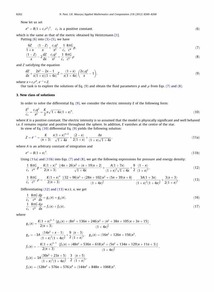
Now let us set

ev ¼ Bð1þ c1r2Þ3; c1 is a positive constant: ð6Þ

which is the same as that of the metric obtained by Heintzmann [1].Putting (6) into (3)–(5), we have

6Z1þ x

� ð1� ZÞx

þ c1q2

x2 ¼1c1

8pGc4 p; ð7Þ

ð1� ZÞx

� 2dZdx� c1q2

x2 ¼1c1

8pGc2 q ð8Þ

and Z satisfying the equation

dZdxþ 2x2 � 2x� 1

xð1þ xÞð1þ 4xÞ Z ¼ð1þ xÞ

xð1þ 4xÞ2c1q2

x� 1

� �; ð9Þ

where x = c1r2, e�k = Z.Our task is to explore the solutions of Eq. (9) and obtain the fluid parameters p and q from Eqs. (7) and (8).

3. New class of solutions

In order to solve the differential Eq. (9), we consider the electric intensity E of the following form:

E2

c1¼ c1q2

x2 ¼K2

xffiffiffiffiffiffiffiffiffiffiffiffiffiffi1þ 4x

pð1þ xÞn; ð10Þ

where K is a positive constant. The electric intensity is so assumed that the model is physically significant and well behavedi.e. E remains regular and positive throughout the sphere. In addition, E vanishes at the centre of the star.

In view of Eq. (10) differential Eq. (9) yields the following solution:

Z ¼ e�k ¼ Kðnþ 3Þ :

xð1þ xÞnþ2ffiffiffiffiffiffiffiffiffiffiffiffiffiffi1þ 4xp þ ð2� xÞ

2ð1þ xÞ þAx

ð1þ xÞffiffiffiffiffiffiffiffiffiffiffiffiffiffi1þ 4xp ; ð11aÞ

where A is an arbitrary constant of integration and

ev ¼ Bð1þ xÞ3: ð11bÞ

Using (11a) and (11b) into Eqs. (7) and (8), we get the following expressions for pressure and energy density:

1c1

8pGc4 p ¼ Kð1þ xÞn

2ðnþ 3Þ :½ð4nþ 26Þx2 þ ðnþ 19Þxþ 2�ffiffiffiffiffiffiffiffiffiffiffiffiffiffi

1þ 4xp þ Að1þ 7xÞ

ð1þ xÞ2ffiffiffiffiffiffiffiffiffiffiffiffiffiffi1þ 4xp þ 9

2:ð1� xÞð1þ xÞ2

; ð12Þ

1c1

8pGc2 q ¼ �Kð1þ xÞn

2ðnþ 3Þ :½ð32þ 96Þx3 þ ð28nþ 102Þx2 þ ð5nþ 39Þxþ 6�

ð1þ 4xÞ32

� 3Að1þ 3xÞð1þ xÞ2ð1þ 4xÞ

32þ 3ðxþ 3Þ

2ð1þ xÞ2: ð13Þ

Differentiating (12) and (13) w.r.t. x, we get

1c1:8pG

c4

dpdx¼ g1ðxÞ þ g2ðxÞ; ð16Þ

1c1:8pG

c2

dqdx¼ f1ðxÞ þ f2ðxÞ; ð17Þ

where

g1ðxÞ ¼Kð1þ xÞn�1

2ðnþ 3Þfg3ðxÞ þ ð8n2 þ 136nþ 246Þx2 þ ðn2 þ 38nþ 105Þxþ 3nþ 15g

ð1þ 4xÞ32

;

g2 ¼ �3Að14x2 þ x� 1Þð1þ xÞ3ð1þ 4xÞ

32þ 9

2ðx� 3Þð1þ xÞ3

; g3ðxÞ ¼ ð16n2 þ 126nþ 156Þx3;

f1ðxÞ ¼ �Kð1þ xÞn�1

2ðnþ 3Þ :ff3ðxÞ þ ð48n2 þ 536nþ 618Þx2 þ ð5n2 þ 134nþ 129Þxþ 11nþ 3Þg

ð1þ 4xÞ52

;

f2ðxÞ ¼ 3Að30x2 þ 23xþ 5Þð1þ xÞ3ð1þ 4xÞ

52� 3

2:ðxþ 5Þð1þ xÞ3

;

f3ðxÞ ¼ ð128n2 þ 576nþ 576Þx4 þ ð144n2 þ 848nþ 1068Þx3:


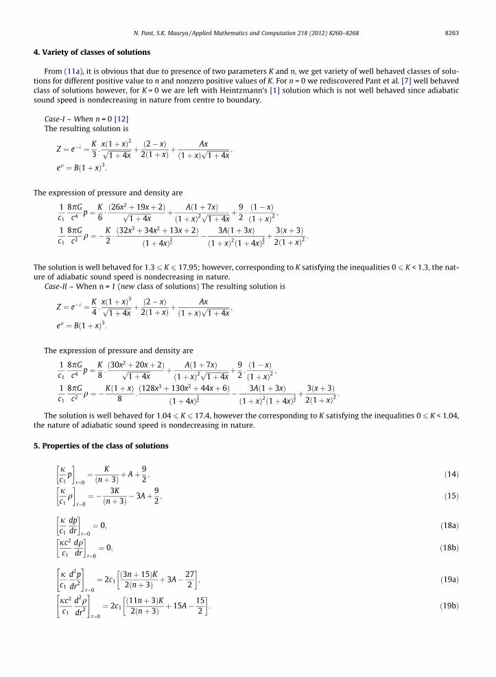
4. Variety of classes of solutions

From (11a), it is obvious that due to presence of two parameters K and n, we get variety of well behaved classes of solu-tions for different positive value to n and nonzero positive values of K. For n = 0 we rediscovered Pant et al. [7] well behavedclass of solutions however, for K = 0 we are left with Heintzmann’s [1] solution which is not well behaved since adiabaticsound speed is nondecreasing in nature from centre to boundary.

Case-I – When n = 0 [12]The resulting solution is

Z ¼ e�k ¼ K3:xð1þ xÞ2ffiffiffiffiffiffiffiffiffiffiffiffiffiffi

1þ 4xp þ ð2� xÞ

2ð1þ xÞ þAx

ð1þ xÞffiffiffiffiffiffiffiffiffiffiffiffiffiffi1þ 4xp ;

ev ¼ Bð1þ xÞ3:

The expression of pressure and density are

1c1

8pGc4 p ¼ K

6� ð26x2 þ 19xþ 2Þffiffiffiffiffiffiffiffiffiffiffiffiffiffi



2� ð1� xÞð1þ xÞ2

;

1c1

8pGc2 q ¼ �K

2� ð32x3 þ 34x2 þ 13xþ 2Þ

ð1þ 4xÞ32


32þ 3ðxþ 3Þ

2ð1þ xÞ2:

The solution is well behaved for 1.3 6 K 6 17.95; however, corresponding to K satisfying the inequalities 0 6 K < 1.3, the nat-ure of adiabatic sound speed is nondecreasing in nature.

Case-II – When n = 1 (new class of solutions) The resulting solution is

Z ¼ e�k ¼ K4:xð1þ xÞ3ffiffiffiffiffiffiffiffiffiffiffiffiffiffi

1þ 4xp þ ð2� xÞ

2ð1þ xÞ þAx

ð1þ xÞffiffiffiffiffiffiffiffiffiffiffiffiffiffi1þ 4xp ;

ev ¼ Bð1þ xÞ3:

The expression of pressure and density are

1c1

8pGc4 p ¼ K

8:ð30x2 þ 20xþ 2Þffiffiffiffiffiffiffiffiffiffiffiffiffiffi




;

1c1

8pGc2 q ¼ �Kð1þ xÞ

8:ð128x3 þ 130x2 þ 44xþ 6Þ

ð1þ 4xÞ32


32þ 3ðxþ 3Þ

2ð1þ xÞ2:

The solution is well behaved for 1.04 6 K 6 17.4, however the corresponding to K satisfying the inequalities 0 6 K < 1.04,the nature of adiabatic sound speed is nondecreasing in nature.

5. Properties of the class of solutions

jc1

p� �

r¼0¼ Kðnþ 3Þ þ Aþ 9

2; ð14Þ

jc1

q� �

r¼0¼ � 3Kðnþ 3Þ � 3Aþ 9

2; ð15Þ

jc1

dpdr

� �r¼0¼ 0; ð18aÞ

jc2

c1

dqdr

� �r¼0¼ 0; ð18bÞ

jc1

d2p

dr2

" #r¼0

¼ 2c1ð3nþ 15ÞK

2ðnþ 3Þ þ 3A� 272

� �; ð19aÞ

jc2

c1

d2qdr2

" #r¼0

¼ 2c1ð11nþ 3ÞK

2ðnþ 3Þ þ 15A� 152

� �: ð19bÞ


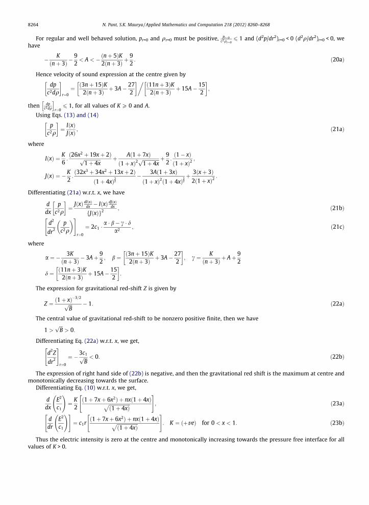
For regular and well behaved solution, pr=0 and qr=0 must be positive, pr¼0c2qr¼0

6 1 and (d2p/dr2)r=0 < 0 (d2q/dr2)r=0 < 0, wehave

� Kðnþ 3Þ �

92< A < �ðnþ 5ÞK

2ðnþ 3Þ þ92: ð20aÞ

Hence velocity of sound expression at the centre given by

dpc2dq

� �r¼0¼ ð3nþ 15ÞK

2ðnþ 3Þ þ 3A� 272

� ��ð11nþ 3ÞK

2ðnþ 3Þ þ 15A� 152

� �;

then dpc2dq

h ir¼06 1, for all values of K P 0 and A.

Using Eqs. (13) and (14)

pc2q

� �¼ IðxÞ

JðxÞ ; ð21aÞ

where

IðxÞ ¼ K6:ð26x2 þ 19xþ 2Þffiffiffiffiffiffiffiffiffiffiffiffiffiffi




;

JðxÞ ¼ �K2:ð32x3 þ 34x2 þ 13xþ 2Þ

ð1þ 4xÞ32


32þ 3ðxþ 3Þ

2ð1þ xÞ2:

Differentiating (21a) w.r.t. x, we have

ddx

pc2q

� �¼

JðxÞ dIðxÞdx � IðxÞ dJðxÞ

dx

fJðxÞg2 ; ð21bÞ

d2

dr2

pc2q

� �" #r¼0

¼ 2c1 �a � b� c � d

a2 ; ð21cÞ

where

a ¼ � 3Kðnþ 3Þ � 3Aþ 9

2; b ¼ ð3nþ 15ÞK

2ðnþ 3Þ þ 3A� 272

� �; c ¼ K

ðnþ 3Þ þ Aþ 92

d ¼ ð11nþ 3ÞK2ðnþ 3Þ þ 15A� 15

2

� �:

The expression for gravitational red-shift Z is given by

Z ¼ ð1þ xÞ�3=2ffiffiffiBp � 1: ð22aÞ

The central value of gravitational red-shift to be nonzero positive finite, then we have

1 >ffiffiffiBp

> 0:

Differentiating Eq. (22a) w.r.t. x, we get,

d2Z

dr2

" #r¼0

¼ �3c1ffiffiffiBp < 0: ð22bÞ

The expression of right hand side of (22b) is negative, and then the gravitational red shift is the maximum at centre andmonotonically decreasing towards the surface.

Differentiating Eq. (10) w.r.t. x, we get,

ddx

E2

c1

!¼ K

2ð1þ 7xþ 6x2Þ þ nxð1þ 4xÞffiffiffiffiffiffiffiffiffiffiffiffiffiffiffiffiffiffi

ð1þ 4xÞp

" #; ð23aÞ

ddr

E2

c1

!" #¼ c1r

ð1þ 7xþ 6x2Þ þ nxð1þ 4xÞffiffiffiffiffiffiffiffiffiffiffiffiffiffiffiffiffiffið1þ 4xÞ

p" #

: K ¼ ðþveÞ for 0 < x < 1: ð23bÞ

Thus the electric intensity is zero at the centre and monotonically increasing towards the pressure free interface for allvalues of K > 0.

Table 1Maximum mass (M/MH) and radius (a) for different n, K and c1a2 for WEC and SEC with well behaved nature.

n K 0 6 p 6 c2q(WEC) 0 6 3p 6 c2q(SEC)

c1a2 Radius (km) Max mass M/MH c1a2 Radius (km) Max mass M/MH

0 1.3 0.3546 16.9057 4.5132 0.3546 16.9057 4.51320.5 1.15 0.3426 16.9746 4.4472 0.3426 16.9746 4.44721 1.04 0.3290 17.0272 4.3710 0.3290 17.0272 4.37101.5 0.97 0.3125 17.0641 4.2750 0.3125 17.0641 4.275010 0.4 0.1884 16.8977 3.2500 0.1884 16.8977 3.250050 0.13 0.0711 14.1521 1.4615 0.0711 14.1521 1.4615100 0.070 0.04295 12.1080 0.8479 0.04295 12.1080 0.8479300 0.0188 0.0188 8.78950 0.3022 0.0188 8.7895 0.302210,000 0.0006 0.000892 2.06598 0.00373 0.000892 2.06598 0.00373

Z = red shift, solar mass MH = 1.475 km, P = (8pG/c4) pa2, D = (8pG/c2) qa2, Q = q, G = 6.673 � 10�8 cm3/g s2, c = 2.997 � 1010 cm/s.

Table 2Pressure (P), density (D), charge (Q), velocity of sound (

ffiffiffiffiffiffiffiffiffiffiffiffiffiffiffiffiffiffidp=c2dq

p), pressure–density ratio (p/c2q) and red-shift (Z) for n = 0.5, K = 1.15 and c1a2 = 0.3426.

n = 0.5, K = 1.15, c1a2 = 0.3426, radius (a) = 16.9746 km, M = 4.4472MH

r/a P D Qffiffiffiffiffiffiffiffiffiffiffiffiffiffiffiffiffiffiffidp=c2dq

pp/c2q Z

0.0 0.7811 3.8236 0.0000 0.6254 0.2043 1.08070.2 0.6984 3.6122 0.0359 0.6253 0.1933 1.03870.4 0.4913 3.0762 0.3006 0.6167 0.1597 0.92070.6 0.2518 2.4024 1.0840 0.5757 0.1048 0.74770.8 0.0687 1.7206 2.7771 0.4586 0.0399 0.54551.0 0.0000 1.0753 5.8900 0.0170 0.0000 0.3375


Table 3Pressure (P), density (D), charge (Q), velocity of sound (


pÞ, pressure–density ratio (p/c2q) and red-shift (Z) for n = 1, K = 1.04 and c1a2 = 0.3290.

n = 1, K = 1.04, c1a2 = 0.3290, radius (a) = 17.0272 km, M = 4.3710MH


pp/c2q Z

0.0 0.7488 3.6755 0.0000 0.6321 0.2037 1.04120.2 0.6717 3.4825 0.0329 0.6320 0.1929 1.00150.4 0.4768 2.9892 0.2782 0.6236 0.1595 0.89000.6 0.2478 2.3607 1.0167 0.5833 0.1050 0.72570.8 0.0688 1.7127 2.6512 0.4660 0.0402 0.53251.0 0.0000 1.0820 5.7450 0.0042 0.0000 0.3323

Z = red shift, solar mass MH = 1.475 km, P = (8pG/c4) pa2, D = (8pG/c2) qa2, Q = q, G = 6.673 � 10�8 cm3/gs2, c = 2.997 � 1010 cm/s.

Table 4Pressure (P), density (D), charge (Q), velocity of sound ð





pp/c2q Z

0.0 0.3634 2.3011 0.0000 0.6535 0.1579 0.63350.2 0.3348 2.2342 0.0119 0.6534 0.1499 0.61520.4 0.2572 2.0511 0.1088 0.6477 0.1254 0.56230.6 0.1519 1.7889 0.4534 0.6170 0.0849 0.48030.8 0.0504 1.4706 1.4211 0.5102 0.0343 0.37701.0 0.0000 1.0656 3.8835 0.0032 0.0000 0.2608

Z = red shift, solar mass MH = 1.475 km, P = (8pG/c4) pa2, D = (8pG/c2) qa2, Q = q, G = 6.673 � 10�8 cm3/gs2, c = 2.997 � 1010 cm/s.


6. Boundary conditions

Besides the above, the charged fluid spheres is expected to join smoothly with the Reissner–Nordstrom metric at the pres-sure free boundary r = a,

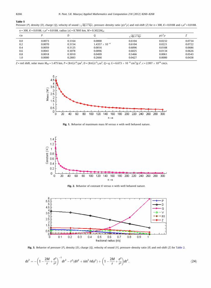
Table 5Pressure (P), density (D), charge (Q), velocity of sound ð





pp/c2q Z

0.0 0.0073 0.3164 0.0000 0.6104 0.0232 0.07340.2 0.0070 0.3154 1.4357 � 10�4 0.6104 0.0221 0.07220.4 0.0059 0.3125 0.0016 0.6096 0.0188 0.06860.6 0.0041 0.3078 0.0096 0.6025 0.0134 0.06260.8 0.0018 0.3010 0.0499 0.5466 0.0061 0.05431.0 0.0000 0.2883 0.2666 0.0427 0.0000 0.0438


Fig. 1. Behavior of maximum mass M versus n with well behaved nature.

Fig. 2. Behavior of constant K versus n with well behaved nature.

Fig. 3. Behavior of pressure (P), density (D), charge (Q), velocity of sound (V), pressure–density ratio (R) and red-shift (Z) for Table 2.


ds2 ¼ � 1� 2Mrþ e2

r2

� ��1

dr2 � r2ðdh2 þ sin2 hd/2Þ þ 1� 2Mrþ e2

r2

� �dt2

; ð24Þ




(where e is total charge on the boundary).which requires the continuity of ek, em and q across the boundary r = a,

e�kðaÞ ¼ 1� 2Maþ e2

a2 ; ð25Þ

emðaÞ ¼ y2ðr¼aÞ ¼ 1� 2M

aþ e2

a2 ; ð26Þ

qðaÞ ¼ e; ð27Þpðr¼aÞ ¼ 0: ð28Þ

The condition (28) can be utilized to compute the values of arbitrary constant A.On setting xr=a = X = Ca2 (a being the radius of the charged sphere).pressure at p(r=a) = 0 gives

A ¼ �Kð1þ XÞnþ2

2 � ðnþ 3Þ �½ð4nþ 26ÞX2 þ ðnþ 26ÞX þ 2�

ð1þ 7XÞ � 92� ð1� XÞ

ffiffiffiffiffiffiffiffiffiffiffiffiffiffiffi1þ 4Xp

ð1þ 7XÞ

" #: ð29Þ

The expression for mass can be written as

M ¼ a2� 1� AX

ð1þ XÞ �ffiffiffiffiffiffiffiffiffiffiffiffiffiffiffi1þ 4Xp � ð2� XÞ

2 � ð1þ XÞ �K � ð1þ XÞn 2X � ð1þ XÞ2 � ðnþ 3ÞX2ð1þ 4XÞ

h i2 � ðnþ 3Þ �

ffiffiffiffiffiffiffiffiffiffiffiffiffiffiffi1þ 4Xp

24

35; ð30Þ

such that e�kðaÞ ¼ 1� 2Ma þ e2

a2, where M = m(a).The condition (26), y2

ðr¼aÞ ¼ 1� 2Ma þ e2

a2 gives

B ¼ Kðnþ 3Þ :

Xð1þ XÞn�1ffiffiffiffiffiffiffiffiffiffiffiffiffiffiffi1þ 4Xp þ ð2� XÞ

2ð1þ XÞ3þ AX

ð1þ XÞ4ffiffiffiffiffiffiffiffiffiffiffiffiffiffiffi1þ 4Xp : ð31Þ

Also, if the surface density qa is prescribed as 2 � 1014 g cm�3(super dense star case), then value of constant c1 can becalculated for a given X(=c1a2), using the following expression:

8pGc2 qa ¼ c1 �

K2:ð32X3 þ 34X2 þ 13X þ 2Þ

ð1þ 4XÞ32

� 3Að1þ 3XÞð1þ XÞ2ð1þ 4XÞ

32þ 3ðX þ 3Þ

2ð1þ XÞ2

" #ð32Þ


7. Conclusions

In the present article, we have derived a family of well behaved charge analogues of neutral super-dense star model dueto Heintzmann [1] by using a particular electric field intensity, which depend upon two parameter K and n. The chargedsuper-dense star models satisfy the energy conditions c2q P 3p > 0, adiabatic index c = ((p + c2q)/p)(dp/(c2dq)) > 1, dp/dr < 0, dq/dr < 0 and the causality condition dp/c2dq < 1 for each non-negative value of n, and K. For well behaved conditionsthe range of K is specified as 1.3 6 K 6 17.95 for n = 1. Table 1 supplies over all the maximum mass and corresponding radiusfor the different parameter K and c1a2. The maximum mass and corresponding radius of the charged super-dense star modelis computed to be 4.5132MH and 16.9057 km respectively with the surface red shift Za = 0.6902 for n = 0. We are also pre-senting the models at the end results for the cases n = 0.5, 1, 10 and 300 and the variation of different physical parametersunder well behaved conditions and maximum mass corresponding to these solutions (Tables 2–5). Further, we observed thatthe value of K is asymptotically approaching to zero as n tends to infinity i.e. the solution is approaching to neutral solutionwith significantly low mass (Figs. 1 and 2). The behavior of physical quantities of Tables 2–4 are shown in Figs. 3–5respectively.

Acknowledgments

One of the authors S.K. Maurya is thankful to ‘‘Ministry of Human Resource Development’’ for the financial support. Theauthors are also really grateful to the honourable referees for his valuable suggestions which could make the paper in thepresentable form. The authors are also acknowledging their gratitude to Prof. Y.K. Gupta, Department of Mathematics, IIT-Roorkee for his motivation and suggestions.

References

[1] H. Heintzmann, Z. Phys. 228 (1969) 489.[2] B.V. Ivanov, Phys. Rev. D 65 (2002) 104001.[3] Y.K. Gupta, M. Kumar, Gen. Relativ. Gravit. 37 (2005) 575.[4] N. Bijalwan, Y.K. Gupta, Astrophys. Space Sci. 317 (2008) 251.[5] Y.K. Gupta, S. Gupta, Pratibha, Int. J. Thoer. Phys. 49 (2010) 854.[6] M.C. Durgapal, R.S. Fuloria, Gen. Relativ. Gravit. 17 (1985) 671.[7] Y.K. Gupta, S.K. Maurya, Astrophys. Space Sci. 331 (2011) 135.[8] S. Thirukkanesh, S.D. Maharaj, Nonlin. Anal. RWA 10 (2009) 3396.[9] K. Komathiraj, S.D. Maharaj, J. Math. Phys. 48 (2007) 042501.

[10] N. Pant et al, Astrophys. Space Sci. 332 (2011) 473.[11] M.S.R. Delgaty, K. Lake, Comp. Phys. Commun. 115 (1998) 395.[12] N. Pant et al, Astrophys. Space Sci. 330 (2010) 353.[13] C. Leibovitz, Phys. Rev. D 185 (1969) 1664.[14] V. Canuto, J. Lodenquai, Phys. Rev. C 12 (1975) 2033.[15] L.D. Landau, E.M. Lifshitz, The Classical Theory of Fields, Pergamon Press, Oxford, England, 1975. p. 255.

relativistic modeling of charged super-dense star with einstein–maxwell equations in general...

Documents