relative prices and wage inequality: evidence from...
TRANSCRIPT

www.elsevier.com/locate/econbase
Journal of International Economics 64 (2004) 387–409
Relative prices and wage inequality:
evidence from Mexico
Raymond Robertson*
Department of Economics, Macalester College, 1600 Grand Avenue, St. Paul, MN 55105-1899, USA
Received 31 October 2001; received in revised form 18 June 2003; accepted 25 June 2003
Abstract
This paper examines the link between relative goods prices and relative wages during two periods
of Mexico’s trade liberalization. The relative price of skill-intensive goods rose following Mexico’s
entrance to the General Agreement and Tariffs and Trade (GATT) in 1986, but fell after Mexico
entered the North American Free Trade Agreement (NAFTA) in 1994. This paper adds a band pass
filter to two established techniques to compare the relationship between prices and wages. Results
from all three approaches are consistent with a positive long-run relationship between relative output
prices and relative wages. The band pass filter results suggest that the relevant time frame for the
relationship begins after 3–5 years.
D 2003 Elsevier B.V. All rights reserved.
Keywords: Trade liberalization; Wage inequality; Mexico
JEL classification: F16; J31
Although over 100 recent papers analyze the relationship between globalization and
wage inequality, the theoretical and empirical link between them remains contested. Starting
with the Stolper–Samuelson theorem, a standard result in trade theory that links changes in
goods prices and changes in relative factor prices, this paper considers two issues that arise in
the trade and wages debate. The first issue is whether changes in relative prices can explain
changes in relative wages and whether changes in tariffs and trade policy explain move-
ments in relative prices. The second is when changes in relative prices affect relative wages.
To examine these two questions, this paper examines Mexico’s trade liberalization.
Revisiting the Mexican case is important for two reasons. Studying the Mexican case may
0022-1996/$ - see front matter D 2003 Elsevier B.V. All rights reserved.
doi:10.1016/j.jinteco.2003.06.003
* Tel.: +1-651-696-6739; fax: +1-651-696-6746.
E-mail address: [email protected] (R. Robertson).

R. Robertson / Journal of International Economics 64 (2004) 387–409388
provide information about the link between trade liberalization and wage inequality
because Mexico is more like the classical ‘‘small country’’ assumed in many trade models.
For example, Mexico’s economy is about 1/17th the size of the United States economy.
While only about 9.1% of U.S. merchandise exports and imports are with Mexico, the
United States accounts for 74.5% of Mexico’s imports and 84.0% of Mexico’s exports.
The true advantage of, and evidence suggestive of, Mexico’s ‘‘small country’’ status is that
the change in relative prices is traced to the ‘‘exogenous’’ shock of tariff reduction. Unlike
the United States, whose changes in relative prices are affected by technology and several
other factors, the speed and extent of Mexico’s liberalization presents a potentially more
direct example of the link between trade liberalization and relative wages through changes
in relative goods prices. Of course, like many Latin American countries implementing
liberalization, Mexico experienced several other changes that could explain wage move-
ments. This paper considers movements in foreign direct investment, real exchange rates,
relative factor supplies, and skill-biased technological change as alternative explanations
for wage changes.
Second, Mexico’s liberalization can be divided into two distinct periods. Mexico first
opened trade to an arguably less-skill abundant world when it joined the General
Agreement and Tariffs and Trade (GATT) in 1986 (Wood, 1997). The main effect of
the GATT was a dramatic reduction in tariffs.1 Mexico further liberalized trade with skill-
abundant Canada and the United States by joining the North American Free Trade
Agreement (NAFTA) in 1994. NAFTA further reduced tariffs and fostered deeper North
American integration by harmonizing standards, facilitating capital flows, and reducing
non-tariff barriers.
This paper uses three approaches to evaluate the link between changes in relative prices
and changes in relative wages in Mexico. I apply both consistency checks (Krueger, 1997;
Lawrence and Slaughter, 1993; Sachs and Shatz, 1994; Schmitt and Mishel, 1996) and
mandated wage equations (Baldwin and Cain, 2000; Baldwin and Hilton, 1984; Haskel
and Slaughter, 2001; Krueger, 1997; Leamer, 1998) found in these price studies. To
evaluate the link between tariff changes and wages directly, I apply the two-stage
modification of the mandated wage approach proposed by Feenstra and Hanson (1999).
I also follow Haskel and Slaughter (2001) by considering possible effects of skill-based
technological change. Third, Slaughter’s (2000) question, ‘‘How fast does the Stolper–
Samuelson clock tick?’’ suggests that time series approaches are relevant for the debate. I
introduce a band pass filter to provide one of the first estimates of the relevant time frame
for the price–wage relationship.
This paper presents three main findings. First, this paper supports and extends earlier
work on Mexico’s trade liberalization (e.g. Hanson and Harrison, 1999; Revenga, 1997;
Cragg and Epelbaum, 1996) and extends these papers by showing that wage inequality
reversed course and began to fall after NAFTA. Second, I find that the relative price of
skill-intensive goods rose following entrance to the GATT, but after NAFTA, the relative
price of skill-intensive goods fell. These price changes are consistent with the change in
1 The maximum effective tariff in manufacturing prior to the GATT was 80%. The maximum tariff prior to
the NAFTA was 20%.

R. Robertson / Journal of International Economics 64 (2004) 387–409 389
tariffs that occurred under the GATT and endowment-based expectations of Mexico’s
integration with its skill-abundant northern neighbors. Hanson and Harrison (1999) find
that Mexico protected less-skill-intensive industries before entering the GATT and tariff
reductions were larger for less-skill-intensive industries, but surprisingly do not find
significant evidence of a link between changes in output prices and wages. Using more
detailed price data, this paper finds strong and consistent evidence of the link that
completes their story. Third, the band pass filter results suggest that the relationship
between relative prices and relative wages emerges in 3–5 years and grows over time.
Alternative explanations for changes in wage inequality, such as changing relative
factor supplies, skill-biased technological change, foreign direct investment, and real
exchange rate appreciation, do not seem to move in ways consistent with theory. The
supply of skilled workers moves in the same direction as the relative wage of skilled
workers, and the sector bias of skill-biased technical change seems to be the opposite as
required by theory to explain changes in relative wages. Real exchange rate movements,
which vary greatly over the sample period, and the December, 1994 devaluation-induced
crisis do not seem to explain movements in relative wages.
The paper has five sections. In Section 1, I briefly review the formal derivation of the
Stolper–Samuelson theorem and discuss previous applications of this theorem in the
literature. These results provide a foundation for the rest of the empirical analysis. In
Section 2, I use three independent data sets to document the change in wage inequality
before and after NAFTA. Section 3 illustrates two established empirical approaches and
Section 4 introduces a new approach to the study the relative price–wage relationship.
Section 5 concludes.
1. Relative prices and relative wages: theory and practice
The neoclassical Heckscher–Ohlin framework suggests that changes in trade policy
affect relative wages (w) through changes in relative goods prices ( p). The Stolper–
Samuelson theorem is a standard result in trade theory and therefore is only briefly
reviewed here (Stolper and Samuelson, 1941). The zero profit conditions are represented
as
cðwÞuaijwi ¼ pi ð1Þ
These conditions are totally differentiated and solved to express the change in factor prices
as a function of product prices. The penultimate result is
p ¼ Hw ð2Þ
in which H is the matrix of factor cost shares and the circumflexes (^) indicate percentage
changes.
The Essential Version of the Stolper–Samuelson theorem is derived neatly when H is
square and invertible (as in the two-good, two-factor case). Inverting H yields a direct
relationship between exogenous domestic prices (regardless of whether prices change due
to trade liberalization or other factors) and endogenous wages. Most empirical studies,

R. Robertson / Journal of International Economics 64 (2004) 387–409390
however, use data from many industries while considering at most four factors. A common
empirical response is to appeal to the Correlation Version of the Stolper–Samuelson
Theorem (Deardorff, 1994). The Correlation Version suggests that goods–price changes
and factor–price changes should be correlated, even though it is impossible to say exactly
which factor return will rise.
Haskel and Slaughter (1998) use a CES production function to derive a specific form of
Eqs. (1) and (2) above. In addition to showing how an increase in the relative price of skill-
intensive goods affects wages, they also show that skill-biased technological change
(SBTC) can also have a similar direct effect on relative wages (assuming away the
secondary effect that SBTC may have on output prices). This approach also suggests that
small changes in relative factor supplies that do not cause production to move out of the
current diversification cone should not affect prices and therefore would not affect relative
wages.
Three broad empirical approaches relate prices and wages in the literature. The first
applies ‘‘consistency checks.’’ The Correlation Version (and more strict interpretations)
suggests that in order for output price changes to increase wage inequality, the relative
price of skill-intensive goods must rise. Studies that examine the factor intensity and
timing of price changes have been called ‘‘consistency checks’’ because positive findings
suggest that changes in prices and changes in wages are consistent with the Stolper–
Samuelson theorem. Haskel and Slaughter (1998) also apply consistency checks to SBTC.
Their specific functional form shows that SBTC will increase the relative wage of skilled
workers, and, for SBTC to be a consistent explanation for rising wage inequality, SBTC
must have risen.
Leamer (1998) uses the term ‘‘mandated wage equations’’ to describe the second
empirical approach. Mandated wage equations predict the change in wages that would be
consistent with Stolper–Samuelson effects. The basis for this approach is the idea that
product–price changes should be proportional to factor–price changes where the factor of
proportion is the vector of the industry’s factor shares, and, since the factor share matrix in
Eq. (2) is not invertible, one can estimate Eq. (2) directly. A wage vector is estimated by
regressing the vector of price changes across time on the factor share matrix. The
estimated vector is then compared to actual wage changes. Feenstra and Hanson (1999)
argue that when the mandated wage equation is fully specified, it becomes an identity that
cannot predict any change in wages other than what actually happened. They propose a
two-stage estimation procedure that can identify the change in wages that is due to changes
in policy, such as tariff changes. Haskel and Slaughter (2000), for example, apply this
technique to estimate the effects of tariff changes on relative wages in the United States.
Francois and Nelson (1998) and Francois et al. (1998) argue that Eq. (2) implies that
prices and wages exhibit a long-run relationship. Applying cointegration techniques, they
find evidence of a relationship between relative prices and relative wages through time in
the United States. Equations like Eq. (2), and the Stolper–Samuelson theorem derived
from them under conditions of perfect factor mobility, are probably best interpreted as
statements about the long run. Unfortunately, the theory provides little help in determining
the length of real time that constitutes the ‘‘long run.’’ To approach this question, I take
three steps. First, I apply several methods to determine the appropriate trend since the trend
term is unknown. In the context of the appropriate trend, I find the intuitive result that

R. Robertson / Journal of International Economics 64 (2004) 387–409 391
relative prices and relative wages are both stationary series. Given stationarity, I then
employ a band pass filter to both series to generate evidence on the relevant timeframe for
the relative price–wage relationship.
2. Relative wages in Mexico 1987–1999
To illustrate the change in wage inequality before and after NAFTA, I use three sources
of data provided by Mexico’s National Institute of Geography, Information, and Statistics
(INEGI): the Mexican Industrial Census for the manufacturing sector, the National Urban
Employment Survey (or ENEU, from its Spanish acronym) from eight Mexican metro-
politan areas2 of Mexico, and the Mexican Monthly Industrial Survey (Encuesta Industrial
Mensual, or EIM).
I draw from the 1986, 1989, 1995, and 1999 Mexican Industrial Censuses, which
provide data from the manufacturing industry for the prior year. The Census contains
information on the employment of production workers (obreros) and non-production
workers (empleados), as well as aggregate payments to each type of worker. I calculate the
employment-weighted non-production/production per-worker wage ratio for census years
1985, 1988, 1994, and 1998.3 The path of relative wages is shown in Fig. 1a. Feenstra and
Hanson (1997) use Mexican industrial census data to show the increase in wage inequality
that followed GATT membership. Fig. 1b is consistent with their figure: wage inequality
increases between 1988 and 1994. After NAFTA, however, wage inequality falls.
To examine wage inequality in manufacturing and all other sectors of the economy, I
calculate both the coefficient of variation of log wages and the 90–10 log wage ratio of
working-age employed males and females using the ENEU. Analogous to the United
States Current Population Surveys, the Mexican ENEU is a quarterly household-level
survey used to calculate unemployment statistics. Fig. 1b shows that both measures follow
a path similar to that in Fig. 1a.4
A third source of data is the Monthly Industrial Survey (EIM). The survey includes
data on production and non-production employment and wages, employment hours for
each worker type, the value of production, and the value of sales. Unfortunately, the data
do not include information on capital or intermediate inputs and do not include firms
with fewer than six workers.5 The survey also excludes firms in the maquiladora
2 Mexico City, Mexico State, Monterrey, Guadalajara, Tijuana, Ciudad Juarez, Nuevo Laredo, andMatamoros.3 Prior to 1988, the census years were evenly divisible by 5.4 Evidence that trade may be linked to the change in the demand for skill may also be identified by
comparing the return to education in Mexico’s border region with Mexico’s interior region. Robertson (2000)
shows that the border region is more affected by United States labor markets than the Mexican interior, which
may be due to migration, transportation costs, capital flows, or trade. The return to education estimated from
Mincerian log-wage equations on a continuous education variable in the border and the interior rises and then falls
in both regions, but the change in the border region occurs closer to the NAFTA date. Similar results are
beginning to emerge from other data sets as well. See Airola and Juhn (2001).5 The data do not include information on temporary or unpaid workers. Unpaid workers include apprentices
and family members. In 1988, unpaid workers made up only about 10% of manufacturing employment.
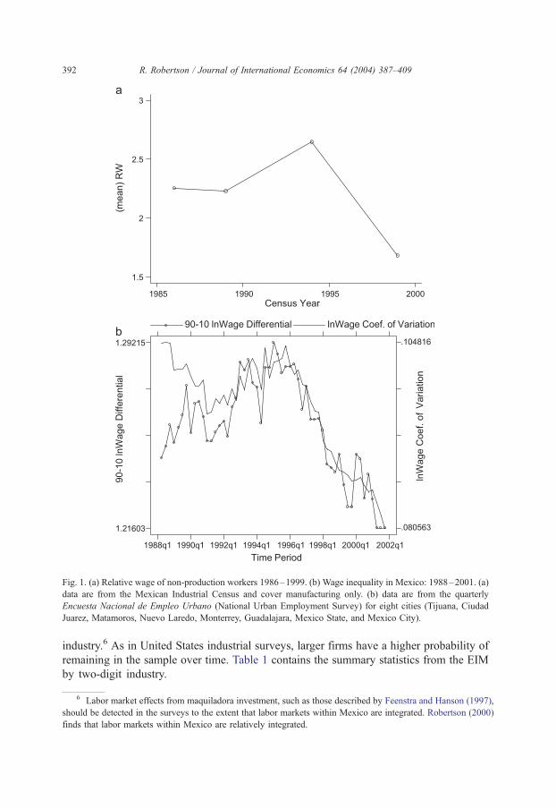
Fig. 1. (a) Relative wage of non-production workers 1986–1999. (b) Wage inequality in Mexico: 1988–2001. (a)
data are from the Mexican Industrial Census and cover manufacturing only. (b) data are from the quarterly
Encuesta Nacional de Empleo Urbano (National Urban Employment Survey) for eight cities (Tijuana, Ciudad
Juarez, Matamoros, Nuevo Laredo, Monterrey, Guadalajara, Mexico State, and Mexico City).
R. Robertson / Journal of International Economics 64 (2004) 387–409392
industry.6 As in United States industrial surveys, larger firms have a higher probability of
remaining in the sample over time. Table 1 contains the summary statistics from the EIM
by two-digit industry.
6 Labor market effects from maquiladora investment, such as those described by Feenstra and Hanson (1997),
should be detected in the surveys to the extent that labor markets within Mexico are integrated. Robertson (2000)
finds that labor markets within Mexico are relatively integrated.

Table 1
Summary statistics of the Mexican monthly industrial survey
Industry Sales Employment Average wage (dollars per hour) H/L Average education (years)
H L Overall H L
Food 45,933.4 182,370.2 4.62 1.54 0.584 8.78 11.72 7.30
Textiles 8,218.5 108,615.4 2.98 1.36 0.323 7.92 10.96 7.28
Wood 966.4 11,389.8 2.84 1.12 0.325 7.97 11.76 7.23
Paper 9,068.5 41,139.8 4.34 1.46 0.383 8.69 11.56 7.75
Chem. 42,270.0 166,318.8 4.97 1.96 0.797 9.86 12.35 8.08
Glass 11,961.2 57,463.6 5.16 1.55 0.420 7.96 12.09 7.02
Metals 24,681.0 57,677.1 4.79 1.77 0.440 8.87 11.75 7.76
Mach. 62,851.0 268,148.3 4.54 1.62 0.512 8.91 11.92 8.07
Other 749.0 7,632.9 4.07 1.33 0.399 8.04 11.07 7.42
Mean 37,547.8 164,793.4 4.40 1.61 0.525 8.76 11.81 7.67
Food represents the food and beverage industry. Textiles includes leather products and apparel. Paper includes
printing. Glass represents all non-metallic minerals (e.g. stone and clay). Metals represents basic metals. ‘‘Mach.’’
represents Metal Products, Machinery, and Equipment, including automobiles. The first five columns of data are
from the Mexican Monthly Industrial Survey. The last three columns of data are from the Mexican National Survey
of Urban Employment. Sales and employment figures are the averages over time of the sums across four-digit
industries within each two-digit industry. Sales figures are in thousands of new pesos. H represents non-production
workers, and L represents production workers. H/L is the ratio of the number of non-production workers to the
number of production workers. Average wages exclude benefits, which are not available by worker type.
R. Robertson / Journal of International Economics 64 (2004) 387–409 393
Following Lawrence and Slaughter (1993), I divide the EIM industries into those that
intensively use production workers and those that intensively use non-production workers.
Use of the production/non-production distinction as a proxy for skill intensity has been
criticized in U.S. studies. In Mexico, however, this distinction seems to capture much of
the skill segregation between industries. To illustrate, the last two columns in Table 1 use
ENEU data to show that production workers have less education in every industry than
non-production workers. Industries with higher relative employment ratios also have
higher average education levels. Both Kendall and Pearson rank-correlation tests reject the
hypothesis that the two measures (education and the non-production/production ratio) are
independent at the 0.0001 level. Using the production/non-production distinction to
(imperfectly) classify skill intensity seems valid in the Mexican case.
The EIM also contains production values and quantities that can be used to compute
unit values. There are 947 identifiable products (averaging 25 products per four-digit
industry). For price data I use unit values calculated from value and volume data.
Quantities for some products were not available. As a result, unit values and price indices
could not be computed over all available products in the industry. In most cases, the share
of the excluded products in the total industry value is relatively small. For industries
missing quantities for certain goods, I constructed the price indices from available unit
prices and dropped industries with no price information.7 For each industry I then
constructed both the Laspeyeres (base-year quantities) and Paasche (current quantities)
7 INEGI constructs and publishes price indices for the two-digit industry level. To test for robustness, I also
used these measures in place of the four-digit constructed price indices. The results are qualitatively similar but, as
expected, the two-digit price indices exhibit much smaller variance.
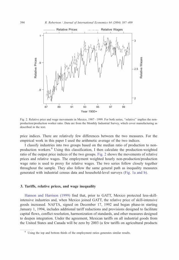
Fig. 2. Relative price and wage movements in Mexico, 1987–1999. For both series, ‘‘relative’’ implies the non-
production/production worker ratio. Data are from the Monthly Industrial Survey, which cover manufacturing as
described in the text.
R. Robertson / Journal of International Economics 64 (2004) 387–409394
price indices. There are relatively few differences between the two measures. For the
empirical work in this paper I used the arithmetic average of the two indices.
I classify industries into two groups based on the median ratio of production to non-
production workers.8 Using this classification, I then calculate the production-weighted
ratio of the output price indices of the two groups. Fig. 2 shows the movements of relative
prices and relative wages. The employment weighted hourly non-production/production
wage ratio is used to proxy for relative wages. The two series follow closely together
throughout the sample. They also follow the same general path as inequality measures
generated with industrial census data and household-level surveys (Fig. 1a and b).
3. Tariffs, relative prices, and wage inequality
Hanson and Harrison (1999) find that, prior to GATT, Mexico protected less-skill-
intensive industries and, when Mexico joined GATT, the relative price of skill-intensive
goods increased. NAFTA, signed on December 17, 1992 and began phase-in starting
January 1, 1994, includes additional tariff reductions and provisions designed to facilitate
capital flows, conflict resolution, harmonization of standards, and other measures designed
to deepen integration. Under the agreement, Mexican tariffs on all industrial goods from
the United States and Canada will be zero by 2003 (a few tariffs on agricultural products
8 Using the top and bottom thirds of the employment ratios generates similar results.

R. Robertson / Journal of International Economics 64 (2004) 387–409 395
will be phased out over 15 years). For tariff reduction purposes, the NAFTA groups United
States and Canadian goods into several categories: those that became duty-free immedi-
ately as of January 1994 (Category A), those that experience five equal reductions of 20%
a year so that these items were duty-free in 1998 (Category B), and those that experience
10 equal reductions of 10% a year, so that these items are duty-free in 2003 (Category C).9
In ordered logit and probit estimation of the likelihood that a product falls into categories
matched to industries in the Mexican Monthly Industrial Survey, the non-production cost
share is negative and significant. In contrast to the GATT, these results imply that
industries with a higher non-production worker ratio experience a more rapid decline in
tariff protection. It would be consistent with the Heckscher–Ohlin framework if broader
integration measures under NAFTA, such as non-tariff barriers, also helped to reduce the
relative price of skill-intensive goods. The time series in Fig. 2 suggest that the relative
price of skilled goods rose after the GATT but fell after NAFTA, but this period is also
characterized by increasing capital flows, rising average worker skill levels, possible skill-
biased technological change, and macroeconomic crisis linked to exchange rate move-
ments. These are discussed in the next section.
3.1. Consistency checks of price movements and skill intensity
To compare price movements over the 1987–1999 period, I first divide the period
using January 1994 as a break point. Following Hanson and Harrison (1999), I deflate the
price data with the Mexican CPI. As in Lawrence and Slaughter (1993), I regress the
change in prices (dPj) over each sample period on the ratio of non-production to
production workers (H/L) at the beginning of each sample period:
dPj ¼ aþ bðH=LÞj þ ej: ð3Þ
Table 2 presents the regression results using Mexican industrial survey data for each
period of trade liberalization.10 Each regression is estimated using weighted least squares
using the mean value of output over 1987–1998 as weights.11 The results suggest that there
is a significant and positive relationship between skill intensity and the change in the output
price for the first period of liberalization (1987–1993 and 1988–1993). This evidence
indicates that the relative price of non-production-worker-intensive goods rose relative to
the price of production-worker-intensive goods. The results are robust to using education as
a measure of skill. The second two columns suggest that the pattern of price change reverses
after NAFTA. The change over the 1993–1998 period is significant at the 10% level and
9 Category D goods were already duty-free before NAFTA, and textiles have slightly different categories. See
http://www.mac.doc.gov/nafta/6000.htm.10 Using U.S. data and without controlling for the computer industry, Lawrence and Slaughter (1993) find
either a negative or zero estimate for b and conclude that the relative price of non-production worker intensive
goods did not increase over the sample period. Using a similar approach and U.S. data, Sachs and Shatz (1994)
control for the computer industry and find a positive correlation. Krueger (1997) uses U.S. data from 1989 to 1995
and finds a positive correlation with and without controlling for the computer industry. Slaughter (2000) discusses
the robustness of results found with and without computer-industry controls.11 Krueger (1997) uses weights and Slaughter (2000) discusses the robustness of using weights. They are
appropriate for the Mexican case because of the large variance in industry employment.
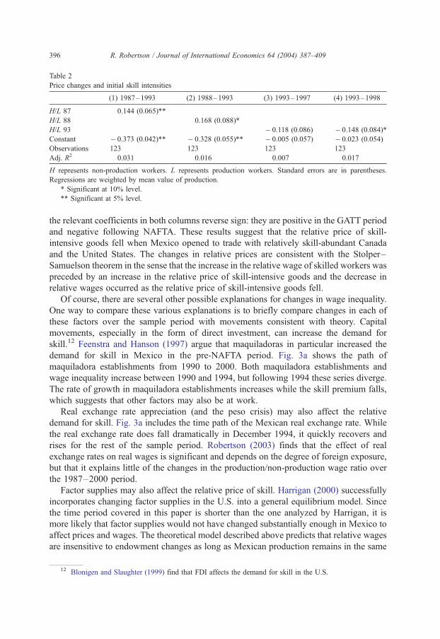
Table 2
Price changes and initial skill intensities
(1) 1987–1993 (2) 1988–1993 (3) 1993–1997 (4) 1993–1998
H/L 87 0.144 (0.065)**
H/L 88 0.168 (0.088)*
H/L 93 � 0.118 (0.086) � 0.148 (0.084)*
Constant � 0.373 (0.042)** � 0.328 (0.055)** � 0.005 (0.057) � 0.023 (0.054)
Observations 123 123 123 123
Adj. R2 0.031 0.016 0.007 0.017
H represents non-production workers. L represents production workers. Standard errors are in parentheses.
Regressions are weighted by mean value of production.
* Significant at 10% level.
** Significant at 5% level.
R. Robertson / Journal of International Economics 64 (2004) 387–409396
the relevant coefficients in both columns reverse sign: they are positive in the GATT period
and negative following NAFTA. These results suggest that the relative price of skill-
intensive goods fell when Mexico opened to trade with relatively skill-abundant Canada
and the United States. The changes in relative prices are consistent with the Stolper–
Samuelson theorem in the sense that the increase in the relative wage of skilled workers was
preceded by an increase in the relative price of skill-intensive goods and the decrease in
relative wages occurred as the relative price of skill-intensive goods fell.
Of course, there are several other possible explanations for changes in wage inequality.
One way to compare these various explanations is to briefly compare changes in each of
these factors over the sample period with movements consistent with theory. Capital
movements, especially in the form of direct investment, can increase the demand for
skill.12 Feenstra and Hanson (1997) argue that maquiladoras in particular increased the
demand for skill in Mexico in the pre-NAFTA period. Fig. 3a shows the path of
maquiladora establishments from 1990 to 2000. Both maquiladora establishments and
wage inequality increase between 1990 and 1994, but following 1994 these series diverge.
The rate of growth in maquiladora establishments increases while the skill premium falls,
which suggests that other factors may also be at work.
Real exchange rate appreciation (and the peso crisis) may also affect the relative
demand for skill. Fig. 3a includes the time path of the Mexican real exchange rate. While
the real exchange rate does fall dramatically in December 1994, it quickly recovers and
rises for the rest of the sample period. Robertson (2003) finds that the effect of real
exchange rates on real wages is significant and depends on the degree of foreign exposure,
but that it explains little of the changes in the production/non-production wage ratio over
the 1987–2000 period.
Factor supplies may also affect the relative price of skill. Harrigan (2000) successfully
incorporates changing factor supplies in the U.S. into a general equilibrium model. Since
the time period covered in this paper is shorter than the one analyzed by Harrigan, it is
more likely that factor supplies would not have changed substantially enough in Mexico to
affect prices and wages. The theoretical model described above predicts that relative wages
are insensitive to endowment changes as long as Mexican production remains in the same
12 Blonigen and Slaughter (1999) find that FDI affects the demand for skill in the U.S.

Fig. 3. (a) Exchange rates and Maquiladora establishments. The real exchange rate is calculated as dollars/peso
nominal exchange rate times the Mexican CPI divided by the U.S. CPI (U.S. and Mexican CPI normalized to 1 in
1986). The maquiladora data are the sum of all establishments in Mexico. Source: http://dgcnesyp.inegi.gob.mx/
bdine/bancos.htm. (b) Supply of skill in Mexico. Each line represents the share of ENEU workers in each
education category.
R. Robertson / Journal of International Economics 64 (2004) 387–409 397
diversification cone. For purposes of consideration, however, we allow the possibility that
all of the changes in relative wages are due to changes in factor supplies, and compare the
movements of factor supplies with the changes in relative wages. The relative shares of
different education groups in the labor force, calculated using ENEU data, are shown in

R. Robertson / Journal of International Economics 64 (2004) 387–409398
Fig. 3b. The relative share of less-skilled workers (workers with less than 10 years of
education) declines over the 1987–1997 period and then increases slightly until 2001. If
anything, the time path of the supply of skilled workers moves in the opposite directions
necessary to explain the observed path of wage inequality.
A fourth alternative is skill-biased technological change (SBTC). Endogenous techno-
logical change could explain changes in inequality if it was significant and changed in
ways consistent with observed changes in inequality. In 1992, INEGI conducted a survey
of 5071 manufacturing firms that inquired about technology investment and acquisition.13
According to the survey, the average share of revenues allocated for research and
development was 0.6% in 1992 while the average share of revenues allocated for
technology purchases was 3.1% in 1992 (up from 2.5% in 1989). Only 2.6% of all firms
in the survey reported using a ‘‘cutting-edge’’ productive process, with the rest having
either a ‘‘mature’’ or ‘‘older’’ process. Developed countries experience relatively more
technological change than Mexico.14
While the extent of technological change in Mexico may be debatable, Canonero and
Werner (2002) argue that SBTC is relevant for Mexico in the first period. Haskel and
Slaughter (1998) [HS] argue that SBTC is not sufficient to explain wage inequality: it is
the sector bias of SBTC that explains changes in relative wages.15 Therefore, I first
estimate skill-biased technological change with Mexican industrial census data and the
methodological approach described by [HS] for industries indexed by k:
DSk ¼ a0 þ a1Dlogðwh=wlÞk þ a2DðK=Y Þk þ ek ; ð4Þ
in which DSk is the change in the non-production employment share in the total wage bill,
wi represents the wage of each worker type, K is capital, and Y is real value-added output,
and the final term is the error. [HS] suggest that skill biased technological change in sector
k can be represented by positive values of a0 + ek. Estimated values from the Mexican
census data are all positive, suggesting that all industries in all periods experienced SBTC
(consistent with Canonero and Werner, 2002). To evaluate the sector bias, [HS] regress
their estimates of SBTC on the initial value of the non-production–production employ-
ment ratio. For this analysis I assume, like [HS], that technology does not affect prices.
The results, available upon request, suggest that the relationship between skill intensity
and SBTC is weakly positive between 1986 and 1989, negative between 1989 and 1994,
and strongly positive from 1994 to 1999. Like the supply of skill, the sector bias of SBTC
is in the opposite direction as would be expected if sector bias matters and SBTC were to
explain the changes in wage inequality.16
13 The National Survey of Employment, Salaries, Technology, and Training in the Manufacturing Sector
(Encuesta Nacional de Empleo, Salarios, tecnologıa y Capacitacion en el Sector manufacturero, 1992) was a joint
project between INEGI, Mexico’s Labor Secretariat, and the OIT.14 For comparison, on average, U.S. industry spent 3.1% of net sales on R&D in 1989 (National Science
Foundation, 1992).15 Xu (2001) finds that the elasticity of substitution may affect these results.16 Several studies have suggesting that decomposing the change in demand for skill into within industry and
between industry components is helpful. Using industrial survey data, the values for this decomposition between
1987 and 1994 are 0.028 = 0.016 + 0.012 and for the 1993–1998 period are � 0.028 =� 0.019–0.009,
suggesting changes both between and within industries over each period.

R. Robertson / Journal of International Economics 64 (2004) 387–409 399
Of the possible explanations considered (capital flows, exchange rate movements,
supply of education, skill-biased technological change, and changes in relative output
prices), changes in relative output prices are the only ones that move in ways consistent
with theory.17 These findings only indirectly support the relationship represented in Eq.
(2). The mandated wage approach provides a potentially more direct alternative.
3.2. The mandated wage approach
To test the long-run relationship between wages and prices, the mandated wage
approach estimates Eq. (2) and compares predicted changes in wages with actual changes.
Baldwin and Cain (2000) implement Eq. (2) with the following regression equation:
pj ¼ a þX
i
wihij þ ej ð5Þ
in which i is the factor index and hij is the share of factor i employed in industry j. The
variables pj and wi represent the output price in industry j and the economy-wide return to
factor i, respectively.18 The estimation deviates from a strict interpretation of the theory in
that the factor shares are the independent variables and the prices are the endogenous
variables. The estimated parameters are the predicted changes in the wages (over the
sample period). A match between the predicted changes and actual changes suggests
support for Stolper–Samuelson effects. A poor match suggests other explanations, such as
changes in technology or an omitted-variable bias.
The U.S. literature identifies four key estimation issues. The first concerns the
exogeneity of price changes. If technology is changing, and technology affects prices,
then failure to account for technology leads to biased results. One advantage of studying
the Mexican case is that prices may be more likely to be exogenous than they are in
the United States in the sense that prices are determined on the world market, trade
policy shocks were relatively large, and technology changes were relatively small. I
therefore maintain the assumption that technology does not have a secondary effect on
prices.
The second estimation issue involves value-added prices. Slaughter (2000) shows that
intermediate inputs make up large and growing shares of production in the U.S.
Accounting for the prices of intermediate inputs is especially important when intermediate
inputs are imported since changes in the prices of intermediate inputs are passed through to
product prices and can thus affect factor prices (Woodland, 1982). Unfortunately, the
industrial survey data do not include information on intermediate inputs. Thus, when using
17 Bell (1997) finds that minimum wages are not binding in Mexico and therefore may not contribute to the
explanation. Maloney and Ribeiro (1999) suggest that unions have little wage-setting power in Mexico. Other
possibilities include other institutional factors, such as the Pactos established in 1987, but a thorough analysis of
these factors seems beyond the scope defined in this paper and is left for future research.18 Here we assume that labor market adjustment costs are small such that factors are perfectly mobile
between industries and, therefore, wages are equalized across industries. Robertson and Dutkowsky (2002) find
that labor market adjustment costs in Mexico are about 1/10 of estimated adjustment costs in the U.S.

R. Robertson / Journal of International Economics 64 (2004) 387–409400
the industrial survey data, I am forced to use ‘‘gross’’ output prices rather than ‘‘net’’
output prices.19
Feenstra and Hanson (1999) introduce two additional estimation issues. First, they
argue that when the mandated wage equation includes inter-industry wage differentials and
productivity, the equation becomes an identity and therefore the estimated coefficients in
Eq. (5) cannot reveal anything about the change in wages other than that which actually
occurred. In Haskel and Slaughter’s (2001) study of U.K. wage inequality, they argue that
inter-industry wage differentials are stable in Great Britain and so do not affect the
analysis. Abuhadba and Romaguera (1993) compare individual level data for Chile,
Uruguay, and Brazil and find ‘‘more similarities than differences’’ with inter-industry
wage differentials observed in U.S. data aggregated over workers, suggesting that inter-
industry wage differentials may be stable in Latin America as well. If inter-industry wage
differentials are stable and technology does not affect prices, then the mandated wage
approach may be appropriate for Mexico.
Second, Feenstra and Hanson (1999) present a two-stage approach to identify the
contribution of the tariff changes on relative wages that I follow below. To begin, however,
I first estimate Eq. (5) for the period following the GATT and again for the period
following the NAFTA. In the first case, I use the average factor shares in 1987 and 1988
and the change in the output price index for each industry over the period 1987–1993 and
1998–1993. In the second case, I use average factor shares from 1993 and 1996 and the
change in the output price index for each industry over the period 1993–1998 and 1996–
1999. I examine the 1996–1999 period because a deep recession began with the collapse
of the peso in December 1994 and began to end in 1996. Following Baldwin and Cain
(2000), I use the value of industry output as regression weights.
The actual changes in average hourly wages and the results from Eq. (5) are found in
Table 3. Although imprecise,20 all of the point estimates are consistent with the Stolper–
Samuelson theorem and the predicted changes are similar to the actual changes. The
predicted changes in wages are larger than the actual changes. In only one case are the
predicted changes statistically different from the actual changes (production workers over
the 1988–1995 period). In this case, the predicted change in wages is large and negative,
while the actual change is close to zero. While the large standard errors make the null
hypothesis (that predicted changes and actual changes are similar) difficult to reject, the
actual wage change for non-production workers is outside the 95% confidence interval for
the predicted wage of production workers in all four cases.
The relative magnitudes reverse following NAFTA, suggesting a predicted fall in wage
inequality. In the period following the crisis, the predicted wage change for both types of
workers is negative. The predicted changes match the actual change in wages in that both
19 To check the robustness of these results, I introduce information on intermediate inputs from the Mexican
Industrial Census. The correlation between the value-added price changes and the gross–output price changes is
0.9033. The findings are qualitatively robust to using value-added prices and accounting for intermediate inputs,
although are less precise due to aggregation in the census.20 The R2 values are generally smaller than those found in U.S. studies. Even for given sample sizes,
Mexican data tend to contain more noise than comparable U.S. data which makes the results somewhat sensitive
to sample and specification.

Table 3
Mandated wage equation results
pj ¼ a þX
i
wihij þ ej
Change in prices over period:
1987–1993 1988–93 1993–1998 1996–1999
Production workers predicted � 1.062 (0.816) � 1.189 (0.876) � 0.679 (1.019) 1.230 (0.669)
actual 0.005 0.164 � 0.243 0.072
p-value 0.193 0.125 0.670 0.086
Non-production workers predicted 2.257 (1.060) 2.134 (1.031) � 1.662 (0.865) 1.190 (0.412)
actual 0.583 0.548 � 0.237 0.039
p-value 0.117 0.126 0.102 0.006
N 127 127 127 127
Adj. R2 0.021 0.018 0.046 0.132
Value of industry production used as weights. Residual input shares (capital, land, and material) were not included
in these regressions. Regressions that included residual input shares produced similar results. Standard errors are
in parentheses.
R. Robertson / Journal of International Economics 64 (2004) 387–409 401
suggest that the relative wage of skilled workers fell following NAFTA. The negative
wage changes are not surprising given the peso-induced recession. The predicted changes
for the 1996–1999 recovery period are positive but again the predicted changes match the
actual wage changes in suggesting a fall in wage inequality. This may be consistent with
the idea that the effects of prices on wages take some time to emerge.
Feenstra and Hanson (1999) argue that a two-stage procedure is necessary to estimate
the contribution of the tariff changes on wages. I follow their approach for the GATT
period using the change in prices over the 1987–1993 period and the 1988–1993 period
as the dependent variable in the first stage regression. Using only the change in tariffs
between 1985 and 1988 for each industry included in the monthly industrial survey as the
independent variable in the first stage, the second stage regression results suggest that the
change in tariffs increased wage inequality.21 The estimated magnitudes are smaller than
both the estimates found in Table 3 and the actual changes. Compared to the actual
changes of non-production worker wages, the results suggest that tariffs explain about a
third of the rise in the non-production worker wage. I analyzed the NAFTA period using
874 product-level prices matched to product-level tariffs. The results from the second stage
regressions suggest that tariffs had a much smaller effect on prices in the NAFTA period
than in the GATT period. Thus, although the fall in the relative price of skilled goods that
followed NAFTA is consistent with the difference in relative endowment of skill, tariffs on
manufactured goods may not have been the primary force driving the change in relative
prices. It is noteworthy, however, that none of the other candidates (capital flows and
SBTC, for example) reverse course after NAFTA in the same way that relative prices do. It
is also possible that we do not know when prices and wages should be related. The next
section generates some results that suggest a timeframe for the relationship between
relative prices and wages.
21 Results available from the author upon request.

R. Robertson / Journal of International Economics 64 (2004) 387–409402
4. The timing of adjustment
Classifying workers as either skilled or unskilled, Francois et al. (1998) circumvent the
dimensionality problem inherent in Eq. (2) by dividing industries into two groups based on
factor intensity. They follow Borjas and Ramey (1994) and Baldwin and Cain (2000)
when constructing their relative wage series and when computing relative prices. Since
there are only two factors (skilled and unskilled workers) and only two goods (based on
factor intensity), the factor share matrix in Eq. (2) can be inverted to yield
w ¼ H�1p; ð6Þwhich Francois et al. (1998) interpret as representing the relationship between relative
prices and relative wages over time. They then test the hypothesis that relative wages
and relative prices are cointegrated. The first of two necessary conditions for
cointegration is that both series must exhibit a unit root. Although there is little
intuitive support for the idea that relative wages and relative prices should be non-
stationary, thoroughness dictates that we consider this first condition. Only if the first
condition is satisfied would we consider whether the difference between the two series
is stationary.
Using the root mean squared error of the regression (RMSE), Akaike’s Information
Criterion (AIC), Amemiya’s Prediction Criterion (PC), and Schwarz’s Information
Criterion (SC), I find that the optimal lag length for prices is 3 and for wages is 4. A
Dickey–Fuller unit root test with these lag lengths and a linear trend fails to reject the unit
root hypothesis for each series.22
The linear trend, however, may not be appropriate for the series shown in Fig. 2. In fact,
the appropriate trend is not known. Since the actual trend is not known, and since it may
affect the unit root tests, I apply strategy S1 suggested by Ayat and Burridge (2000). They
suggest estimating the following equation(s) in which t represents a time trend and y
represents wages or prices:
Dyt ¼ ðq � 1Þyt�1 þ a1 þ a2t þ a3t2 þ
Xs
j¼1
ajDyt�j þ et ð7Þ
These results are presented in Table 4. Since the null of a unit root is rejected, Ayat and
Burridge (2000) suggest next testing the significance of the coefficient on the trend terms
using standard tables to evaluate the t-statistics on the a2 terms. These results are also
shown in Table 4. Since the unit root is rejected and the quadratic trend term is not
rejected, we stop, since this test is ‘‘the only one available which is invariant to the
maintained quadratic trend’’ (Ayat and Burridge, 2000, p. 78).
Instead of a quadratic trend, one may consider that the series are better characterized by
a breaking linear trend. The actual date for this break is unknown, and therefore we are
interested in testing for a unit root in a series with an unknown break. A relatively large
literature addresses this problem. Vogelsang and Perron (1998) refine the methodology for
22 The test statistics ( p-values) are � 2.11 (0.242) and � 2.39 (0.145).

Table 4
Unit root test results
Dyt ¼ ðq � 1Þyt�1 þ a1 þ a2t þ a3t2 þ
Xs
j¼1
ajDyt�j þ et
Prices Prices Prices Wages Wages Wages
(q� 1) � 0.089
(2.345)
� 0.123
(2.543)
� 0.272
(3.952)
� 0.048
(2.527)
� 0.058
(1.581)
� 0.874
(6.324)
a1 0.079
(2.365)
0.047
(1.102)
� 4.998
(2.942)
0.139
(2.713)
0.075
(0.384)
� 91.699
(6.073)
a2 0.001
(1.130)
0.110
(2.988)
0.001
(0.337)
1.956
(6.081)
a3 (�10) � 0.001
(2.971)
� 0.010
(6.078)
a1 � 0.291
(1.615)
� 0.240
(1.290)
� 0.039
(0.204)
� 0.826
(3.266)
� 0.787
(2.831)
0.691
(1.985)
a2 0.003
(0.016)
� 0.036
(0.173)
� 0.183
(0.877)
0.145
(0.332)
0.094
(0.204)
� 1.490
(3.051)
a3 0.055
(0.671)
0.066
(0.803)
0.106
(1.307)
� 0.039
(0.127)
� 0.011
(0.034)
0.867
(2.702)
a4 0.051
(0.626)
0.045
(0.537)
� 0.150
(1.851)
Observations 152 152 152 151 151 151
Adj. R2 0.098 0.100 0.145 0.404 0.400 0.520
Absolute values of t-statistics are in parentheses. The absolute value for the 5% DF test statistic is 2.89 without a
trend term and 3.45 with a trend term. The absolute value for the 5% test statistic with a quadratic trend is between
3.48 and 3.61.
R. Robertson / Journal of International Economics 64 (2004) 387–409 403
identifying an unknown break and testing for unit roots. They consider several different
models. Of these, I apply the following model using the time trend t:
yt ¼ l þ bt þ hDUt þ cDTt þ y2t
y2t ¼Xk
i¼0
xiDðTbÞt�i þ ay2t�1 þXk
i¼0
ciDy2t�i þ ut; ð8Þ
in which DU= 1(t>Tb), DT= 1(t>Tb)(t� Tb), and D(Tb) = 1(t = Tb + 1). I choose this model
because the unit root tests are sensitive to the assumption of a gradual vs. a sharp trend
break, and this problem is magnified when the break in the trend is large (as in the present
case). Using the break points found by minimizing the negative value of c,23 the 5%
critical value for the unit root test of a = 1 is � 4.28. The t-value on the test that a = 1 for
the relative wage series is � 5.06 and for the relative price series is � 4.51. These results
suggest that considering a breaking trend rather than the quadratic trend does not
qualitatively affect the unit root results described earlier. I find no robust evidence of
nonstationarity, so the cointegration approach is not appropriate. I therefore introduce a
new approach to the literature: the band pass filter.
To get an idea of the frequency at which prices and wages are related, we appeal to the
theory of spectral analysis of time series. This theory has been applied primarily in
23 We seek the largest negative t-statistic for the c parameter because we know that the break is negative.
R. Robertson / Journal of International Economics 64 (2004) 387–409404
macroeconomics to separate ‘‘short run’’ relationships (high frequency) from ‘‘long run’’
relationships (low frequency). A tool used to isolate the different frequency components in
time series is the ideal band pass filter. The ideal band pass filter applies a linear
transformation to a series that removes all variation except that which occurs at the
frequency of interest. The ideal band pass filter, unfortunately, requires an infinite series.
Christiano and Fitzgerald (1999) present an approximation to the ideal band pass filter and
apply this approximation to various macroeconomic time series to illustrate whether series
are related in the short or long term.
The filter uses raw data (such as that represented by a series x of actual length T) to
isolate the frequency component y by estimating the B parameters in the following
equations (Eqs. (1.2) and (1.3) in Christiano and Fitzgerald, 1999):
yt ¼ B0xt þ B1xtþ1 þ . . .þ BT�1�txT�1 þ BT�txt þ B1xt�1 þ . . .þ Bt�2x2 þ Bt�1x1
ð9Þin which24
Bj ¼sinð jbÞ � sinð jaÞ
pj; jz 1
B0 ¼b� a
p; a ¼ 2p
pu; b ¼ 2p
pl: ð10Þ
The first step is to detrend the two series. I then use the band pass filter to isolate the
components of relative wages and relative prices that occur at 6–12 months, 1–3 years,
and 3–5 years. I compare these results with the quadratic trends estimated over the whole
sample. The quadratic-detrended series and the components that occur at the 6–12 month
frequency (the latter derived using the filter) show no clear relationship between relative
wages and relative prices. This is not surprising. As Magee (1980) suggests, the Stolper–
Samuelson theorem probably does not hold in the short run. Since the Stolper–Samuelson
theorem assumes that adjustment costs are zero, it is essentially a ‘‘long-run’’ theorem.
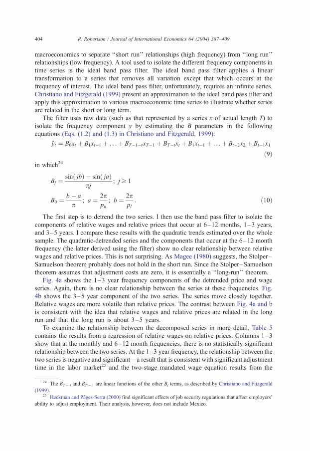
Fig. 4a shows the 1–3 year frequency components of the detrended price and wage
series. Again, there is no clear relationship between the series at these frequencies. Fig.
4b shows the 3–5 year component of the two series. The series move closely together.
Relative wages are more volatile than relative prices. The contrast between Fig. 4a and b
is consistent with the idea that relative wages and relative prices are related in the long
run and that the long run is about 3–5 years.
To examine the relationship between the decomposed series in more detail, Table 5
contains the results from a regression of relative wages on relative prices. Columns 1–3
show that at the monthly and 6–12 month frequencies, there is no statistically significant
relationship between the two series. At the 1–3 year frequency, the relationship between the
two series is negative and significant—a result that is consistent with significant adjustment
time in the labor market25 and the two-stage mandated wage equation results from the
24 The BT� t and BT� 1 are linear functions of the other Bj terms, as described by Christiano and Fitzgerald
(1999).25 Heckman and Pages-Serra (2000) find significant effects of job security regulations that affect employers’
ability to adjust employment. Their analysis, however, does not include Mexico.

Fig. 4. (a,b) Relative price and wage movements in Mexico, 1987–1999, band pass filter results. For both
series, ‘‘relative’’ implies the non-production/production worker ratio. Data are from the Monthly Industrial
Survey, which cover manufacturing as described in the text.
R. Robertson / Journal of International Economics 64 (2004) 387–409 405
immediate post-NAFTA period. Although the coefficient on relative prices is significant, the
adjusted R2 is less than 0.05. In contrast to the short-run frequencies, the 3–5 year
components of relative prices and relativewages are significantly positively related. Relative
prices explain a great deal of the movement in relative wages, as suggested by the adjusted
R2 of over 0.65.

Table 5
Bivariate regressions of wages on prices
w ¼ H�1p
Detrended series 6–12 months 12–36 months 36–60 months
H� 1 0.185 (1.024) � 0.183 (0.738) � 0.245 (2.630) 1.146 (17.859)
Adj. R2 0.000 � 0.003 0.037 0.672
N 156 156 156 156
Absolute value of t-statistics in parentheses.
R. Robertson / Journal of International Economics 64 (2004) 387–409406
To explore robustness, I also examined alternative frequencies, such as 2–4 years.
Frequencies below the 3–5 year range do not generate any significant positive relation-
ship. Another alternative is to consider two periods—a ‘‘short’’ run of 1–3 years and a
‘‘long’’ run of greater than 3 years. Subtracting the ‘‘short’’ run variation from the original
detrended series generates the ‘‘long’’ run series. As in the earlier figures, the ‘‘short’’ run
graphs generate no clear relationship between prices and wages. The ‘‘long’’ run series,
however, exhibit a much closer relationship as shown in Fig. 5. These results suggest that
the 3–5 year frequency is a lower bound to the time frame in which the price and wage
relationship emerges in Mexico. The adjusted R2 in the regression of the quadratic trend of
wages on the quadratic trend of prices is over 0.90. These results suggest that the
relationship between relative prices and relative wages first emerges over the 3–5 year
period and grows over time.
Fig. 5. Relative price and wage Movements in Mexico, 1987–1999, band pass filter results. For both series,
‘‘relative’’ implies the non-production/production worker ratio. Data are from the Monthly Industrial Survey,
which cover manufacturing as described in the text.
R. Robertson / Journal of International Economics 64 (2004) 387–409 407
5. Conclusions
One area of debate in the trade and wages literature is whether changes in product
prices can explain changes in wage inequality as trade theory predicts. Mexico, a small,
recently liberalized economy, offers two different policy changes. First, Mexico liberalized
trade with an arguably less-skill abundant world when it joined the GATT in 1986. Prior to
GATT, Mexico protected less-skill intensive industries. Following entrance to the GATT,
the relative price of skill-intensive goods rose and, consistent with the predictions of the
Stolper–Samuelson theorem, the relative wage of skilled workers rose. Second, when
Mexico further liberalized trade with Canada and the United States, two nations that are
skill abundant relative to Mexico, the relative price of skill-intensive goods fell. Again,
consistent with the predictions of the Stolper–Samuelson theorem, the relative wage of
skilled workers fell after NAFTA.
To examine the link between changes in relative prices and changes in relative wages,
this paper applies two techniques found in the literature and adds a new time-series
approach. All three techniques generate consistent results that suggest that changes in
relative prices and changes in relative wages are related. The third approach, the band pass
filter, provides some of the first evidence about the timing of the Stolper–Samuelson
effects. The band pass filter results suggest that the relationship between prices and wages
begins to emerge in the 3–5-year range and grows stronger over time.
Acknowledgements
The author thanks Antoni Estevadeordal, Terry Fitzgerald, Gordon Hanson, Chihwa
Kao, Gary Krueger, Ed Leamer, J. David Richardson, Matt Slaughter, M. Scott Taylor,
Sarah West, Bin Xu, participants at the 1998 Empirical Investigations in International
Trade conference, the Summer 2001 NBER International Workshop, ITAM, U-Il
Champaign-Urbana, Federal Reserve Bank of Dallas, Georgia Tech, IBMEC (Rio), the
IDB, and two anonymous referees for comments that greatly improved the paper. I also
thank Lic. Ramon Sanchez T. and Lic. Abegael Duran of INEGI for data assistance.
Brendan Bell, Miguel Nieto, Vinicius Pabon, and Sebastian Sanchez de Lozada provided
excellent research assistance. The author accepts sole responsibility for any remaining
errors and gratefully acknowledges financial support from the Latin American and Iberian
Institute at the University of New Mexico and the National Science Foundation.
References
Abuhadba, M., Romaguera, P., 1993. Inter-industry wage differentials: evidence from Latin American countries.
Journal of Development Studies 301, 190–205.
Airola, J., Juhn, C., 2001. Income and Consumption Inequality in Post Reform Mexico. Paper presented at the
2001 Latin American and Caribbean Economic Society Meetings.
Ayat, L., Burridge, P., 2000. Unit root tests in the presence of uncertainty about the non-stochastic trend. Journal
of Econometrics 951, 71–96.
Baldwin, R.E., Cain, G.G., 2000. Shifts in relative U.S. wages: the role of trade, technology, and factor endow-
ments. Review of Economics and Statistics 824, 580–595.

R. Robertson / Journal of International Economics 64 (2004) 387–409408
Baldwin, R., Hilton, R., 1984. A technique for indicating comparative costs and predicting changes in trade
ratios. Review of Economics and Statistics 661, 105–110.
Bell, L., 1997. The impact of minimum wages in Mexico and Colombia. Journal of Labor Economics 153 (Pt. 2),
S102–S135.
Blonigen, B., Slaughter, M., 1999. Foreign-Affiliate Activity and U.S. Skill Upgrading. NBER Working Paper
No. W7040.
Borjas, G., Ramey, V., 1994. Time-series evidence on the sources of trends in wage inequality American.
Economic Review 842, 10–16.
Canonero, G., Werner, A., 2002. Salarios Relativos y Liberacion del Comercio en Mexico. El Trimestre Eco-
nomico 69273, 123–142.
Christiano, L.J., Fitzgerald, T. J., 1999. The Band Pass Filter. NBER Working Paper No. W7257.
Cragg, M., Epelbaum, M., 1996. Why has wage dispersion grown in Mexico? Is it the incidence of reforms or the
growing demand for skills? Journal of Development Economics 51, 99–116.
Deardorff, A., 1994. Overview of the Stolper–Samuelson Theorem. In: Deardorff, A., Stern, R. (Eds.), The
Stolper–Samuelson Theorem: A Golden Jubilee. University of Michigan Press, Ann Arbor, pp. 7–34.
Feenstra, R.C., Hanson, G.H., 1997. Foreign direct investment and relative wages: evidence from Mexico’s
maquiladoras. Journal of International Economics 42, 371–393.
Feenstra, R.C., Hanson, G.H., 1999. The impact of outsourcing and high-technology capital on wages: Estimates
for the United States, 1979–1990. Quarterly Journal of Economics 1143, 907–940.
Francois, J.F., Nelson, D., 1998. Trade, technology, and wages: general equilibrium mechanics. Economic
Journal 108450, 1483–1499.
Francois, J., Navia, R., Nelson, D., 1998. Treating the SS theorem Seriously: The Long-Run Relationship
between Relative Commodity Prices and Relative Factor Prices. Mimeo, Erasmus University.
Hanson, G.H., Harrison, A., 1999. Trade, technology, and wage inequality. Industrial and Labor Relations
Review 522, 271–288.
Harrigan, J., 2000. International trade and American wages in general equilibrium, 1967–1995. In: Feenstra,
R.C. (Ed.), The Impact of International Trade on Wages NBER Conference Report Series. University of
Chicago Press, Chicago, pp. 171–193.
Haskel, J., Slaughter, M.J., 1998. Does the Sector Bias of Skill-Biased Technical Change Explain Changing Wage
Inequality? NBER Working Paper No. 6565.
Haskel, J., Slaughter, M.J., 2000. Have Falling Tariffs and Transportation Costs Raised U.S. Wage Inequality?
NBER Working Paper No. 7539.
Haskel, J., Slaughter, M.J., 2001. Trade, technology and U.K. wage inequality. Economic Journal 111468,
163–187.
Heckman, J., Pages-Serra, C., 2000. The cost of job security regulation: evidence from Latin American labor
markets. Economia 11, 109–144.
Krueger, A., 1997. Labor Market Shifts and the Price Puzzle Revisited. NBER Working Paper No. 5924.
Lawrence, R., Slaughter, M., 1993. International trade and American wages in the 1980s: giant sucking sound or
small hiccup? Brookings Papers: Microeconomics 2, 161–226.
Leamer, E.E., 1998. In search of Stolper–Samuelson linkages between trade and lower wages. In: Collins, S.
(Ed.), Imports, Exports, and the American Worker. Brookings Institute Press, Washington, DC, pp. 141–202.
Magee, S., 1980. Three simple tests of the Stolper–Samuelson Theorem as found. In: Deardorff, A., Stern, R.
(Eds.), The Stolper–Samuelson theorem: A Golden Jubilee. Studies in International Trade Policy. University
of Michigan Press, Ann Arbor, pp. 185–200.
Maloney, W.F., Ribeiro, E.P., 1999. Efficiency Wage and Union Effects in Labor Demand and Wage
Structure in Mexico: An Application of Quantile Analysis. World Bank Policy Research Working Paper
2131.
National Science Foundation, 1992. Research and Development in Industry, 1989. NSF 92-307. Washington, DC,
Government Printing Office.
Revenga, A., 1997. Employment and wage effects of trade liberalization: the case of Mexican manufacturing.
Journal of Labor Economics 153 (Pt. 2), S20–S43.
Robertson, R., 2000. Wage shocks and North American labor-market integration. American Economic Review
904, 742–764.

R. Robertson / Journal of International Economics 64 (2004) 387–409 409
Robertson, R., 2003. Exchange rates and relative wages: evidence from Mexico. The North American Journal of
Economics and Finance 141, 25–48.
Robertson, R., Dutkowsky, D.H., 2002. Labor adjustment costs in a destination country: the case of Mexico.
Journal of Development Economics 671, 29–54.
Sachs, J., Shatz, H., 1994. Trade and jobs in U.S. Manufacturing. Brookings Papers on Economic Activity I,
1–84.
Schmitt, J., Mishel, L., 1996. Did International Trade Lower Less-Skilled Wages During the 1980s? Standard
Trade Theory and Evidence Economic Policy Institute. Technical Paper No. 213.
Slaughter, M., 2000. What are the results of product–price studies and what can we learn from their differences?
In: Feenstra, R.C. (Ed.), The Impact of International Trade on Wages. National Bureau of Economic Research
Conference, vol. 2000, pp. 129–170.
Stolper, W., Samuelson, P., 1941. Protection and real wages. Review of Economic Studies 9, 58–73.
Vogelsang, T., Perron, P., 1998. Additional tests for a unit root allowing for a break in the trend function at an
unknown time. International Economic Review 39 (4), 1073–1100.
Wood, A., 1997. Openness and wage inequality in developing countries: the Latin American challenge to East
Asian conventional wisdom. World Bank Economic Review 111, 33–57.
Woodland, A.D., 1982. International Trade and Resource Allocation. North-Holland, Amsterdam.
Xu, B., 2001. Factor bias, sector bias, and the effects of technical progress on relative factor prices. Journal of
International Economics 541, 5–25.