relative bioavailability of arsenic in the flat creek soil ... bioavailability of arsenic in the...

Relative Bioavailability of Arsenic in the

Flat Creek Soil Reference Material

United States OLEM 9200.2-159 Environmental Protection Agency

Relative Bioavailability of Arsenic in the Flat Creek Soil Reference Material

December 2015

Prepared by:

Stan W. Casteel, DVM, PhD, DABVT

Laura Naught, MS

Veterinary Medical Diagnostic Laboratory

College of Veterinary Medicine

University of Missouri, Columbia

Columbia, Missouri

and

Amber Bacom, MS

William Brattin, PhD

SRC, Inc.

Denver, Colorado

December 9, 2015

OLEM 9200.2-159 December, 2015.doc ii

ACRONYMS AND ABBREVIATIONS

ABA Absolute bioavailability

AFo Oral absorption fraction

ANOVA Analysis of variance

As Arsenic

As+3 Trivalent inorganic arsenic

As+5 Pentavalent inorganic arsenic

DMA Dimethyl arsenic

D Ingested dose

DF Degrees of freedom

FCRM Flat Creek Soil Reference Material

g Gram

GLP Good Laboratory Practices

ICP-MS Inductively coupled plasma-mass spectrometry

ICP-OES Inductively coupled plasma-optical emission spectrometry

Kb Fraction of absorbed arsenic that is excreted in the bile

kg Kilogram

Kt Fraction of absorbed arsenic that is retained in tissues

Ku Fraction of absorbed arsenic that is excreted in urine

MBW Mean body weight

mL Milliliter

MMA Monomethyl arsenic

MSE Mean squared error

N Number of data points

NRC National Research Council

ORD Office of Research and Development

OSRTI Office of Superfund Remediation and Technical Innovation

PE Performance evaluation

QC Quality control

RBA Relative bioavailability

ref Reference material

RfD Reference dose

RPD Relative percent difference

SD Standard deviation

SF Slope factor

SSE Sum of squared standard error

TM Test material

UEF Urinary excretion fraction

U.S. EPA United States Environmental Protection Agency

USGS United States Geological Survey

μg Microgram

°C Degrees Celsius

°F Degrees Fahrenheit

OLEM 9200.2-159 December, 2015.doc iii

TABLE OF CONTENTS

EXECUTIVE SUMMARY ............................................................................................................ v

INTRODUCTION .......................................................................................................................... 1

1.1 Overview of Bioavailability .................................................................................... 1

1.2 Using RBA Data to Refine Risk Calculations ........................................................ 2

1.3 Purpose of this Study .............................................................................................. 2

2.0 STUDY DESIGN................................................................................................................ 2

2.1 Test Materials.......................................................................................................... 3

2.1.1 Sample Description ..................................................................................... 3

2.1.2 Sample Preparation and Analysis ............................................................... 3

2.2 Experimental Animals ............................................................................................ 3

2.3 Diet .......................................................................................................................... 4

2.4 Dosing ..................................................................................................................... 4

2.5 Collection and Preservation of Urine Samples ....................................................... 5

2.6 Arsenic Analysis ..................................................................................................... 5

2.7 Quality Control ....................................................................................................... 5

3.0 Data Analysis ...................................................................................................................... 7

3.1 Overview ................................................................................................................. 7

3.2 Data Fitting ............................................................................................................. 9

3.3 Calculation of RBA Estimates .............................................................................. 12

4.0 RESULTS ......................................................................................................................... 12

4.1 Clinical Signs ........................................................................................................ 12

4.2 Dosing Deviations ................................................................................................. 12

4.3 Background Arsenic Excretion ............................................................................. 12

4.4 Urinary Arsenic Variance ..................................................................................... 13

4.5 Dose-Response Modeling ..................................................................................... 13

4.6 Calculated RBA Values ........................................................................................ 20

4.7 Uncertainty ............................................................................................................ 20

5.0 REFERENCES ................................................................................................................. 21

OLEM 9200.2-159 December, 2015.doc iv

LIST OF TABLES

Table 2-1. Study Design and Dosing Information ......................................................................... 3 Table 4-1. NAXCEL Treatments ................................................................................................. 12

Table 4-2. Background Urinary Arsenic ...................................................................................... 13 Table 4-3. Urine Excretion Fraction (UEF) Estimates ................................................................ 15 Table 4-4. Estimated Arsenic Relative Bioavailability (RBA) for FCRM Soil .......................... 20

LIST OF FIGURES

Figure 3-1. Conceptual Model for Arsenic Toxicokinetics ........................................................... 8

Figure 3-2. Urinary Arsenic Variance Model .............................................................................. 11 Figure 4-1. FCRM Data Compared to Urinary Arsenic Variance Model .................................... 14 Figure 4-2. FCRM Urinary Excretion of Arsenic: Days 6/7 ...................................................... 16 Figure 4-3. FCRM Urinary Excretion of Arsenic: Days 9/10 .................................................... 17

Figure 4-4. FCRM Urinary Excretion of Arsenic: Days 12/13 .................................................. 18 Figure 4-5. FCRM Urinary Excretion of Arsenic: All Days ...................................................... 19

APPENDICES

Appendix A: Group Assignments .............................................................................................. A-1

Table A-1. Group Assignments for FCRM Arsenic Study ................................ A-2

Appendix B: Body Weights ....................................................................................................... B-1 Table B-1. Body Weights .................................................................................... B-2

Appendix C: Typical Feed Composition ................................................................................... C-1 Table C-1: Procine Grower Produced by the University of Missouri Feed

Mill ....................................................................................................................... C-2

Appendix D: Urinary Arsenic Analytical Results and Urine Volumes for FCRM Study

Samples ................................................................................................................ D-1

Table D-1. Urinary Arsenic Analytical Results and Urine Volumes for ............ D-2 Appendix E: Analytical Results for Quality Control Samples ................................................... E-1

Table E-1. Blind Duplicate Samples .................................................................... E-2

Table E-2. Laboratory Spikes ............................................................................... E-2 Table E-3. Laboratory Quality Control Standards ............................................... E-3

Table E-4. Arsenic Performance Evaluation Samples ......................................... E-3 Table E-5. Blanks ................................................................................................. E-4

Figure E-1. Urinary Arsenic Blind Duplicates ..................................................... E-4 Figure E-2. Performance Evaluation Samples ..................................................... E-5

OLEM 9200.2-159 December, 2015.doc v

EXECUTIVE SUMMARY

A study using juvenile swine as test animals was performed to measure the gastrointestinal

absorption of arsenic (As) from a sample of the Flat Creek Soil Reference Material (FCRM). In

conjunction with the United States Environmental Protection Agency (U.S. EPA) Office of

Superfund Remediation and Technology Innovation (OSRTI), FCRM was developed by the

United States Geological Survey (USGS) from soil containing high concentrations of metals due

to mining activity near an abandoned lead mine in Montana. The measured arsenic

concentration of FCRM is 740 ± 57 mg/kg (mean ± standard deviation [SD]).

The relative oral bioavailability of arsenic in FCRM was assessed by comparing the absorption

of arsenic from FCRM (“test material”) to that of a reference material, sodium arsenate. Groups

of swine (five per dose group) were given oral doses of the reference material or the test material

twice a day for 14 days at three target dose levels (40, 80, and 120 mg As/kg body weight/day).

A group of three untreated swine served as a control for the arsenic test groups.

The amount of arsenic absorbed by each animal was evaluated by measuring the amount of

arsenic excreted in the urine (collected over 48-hour periods beginning on days 6, 9, and 12).

The urinary excretion fraction (UEF) is the ratio of the amount excreted per 48 hours divided by

the dose given per 48 hours. UEFs were calculated for the test material and sodium arsenate

using simultaneous weighted linear regression. The relative bioavailability (RBA) of arsenic in

the test material compared to sodium arsenate was calculated as follows:

)(

)(

arsenatesodiumUEF

soiltestUEFRBA

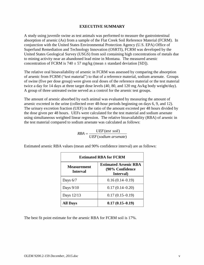
Estimated arsenic RBA values (mean and 90% confidence interval) are as follows:

Estimated RBA for FCRM

Measurement

Interval

Estimated Arsenic RBA

(90% Confidence

Interval)

Days 6/7 0.16 (0.14–0.19)

Days 9/10 0.17 (0.14–0.20)

Days 12/13 0.17 (0.15–0.19)

All Days 0.17 (0.15–0.19)

The best fit point estimate for the arsenic RBA for FCRM soil is 17%.

OLEM 9200.2-159 December, 2015.doc 1

INTRODUCTION

1.1 Overview of Bioavailability

Reliable analysis of the potential hazard to humans from ingestion of a chemical depends upon

accurate information on a number of key parameters, including the concentration of the chemical

in the exposure medium of interest (e.g., soil, dust, water, food, air, paint), intake rates of each

exposure medium, and the rate and extent of absorption (“bioavailability”) of the chemical by the

body from each ingested medium. The amount of a chemical that actually enters the body from

an ingested medium depends on the physical-chemical properties of the chemical and of the

exposure medium. For example, some metals in soil may exist, at least in part, as poorly water-

soluble minerals, and may also exist inside particles of inert matrices such as rock or slag of

variable sizes, shapes, and compositions. These chemical and physical properties may influence

(usually decrease) the absorption (bioavailability) of the metals when ingested. Thus, equal

ingested doses of different forms of a chemical in different media may not be of equal health

concern.

Bioavailability of a chemical in a particular medium may be expressed either in absolute terms

(absolute bioavailability) or in relative terms (relative bioavailability).

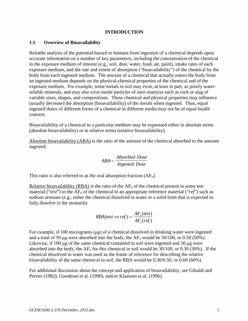
Absolute bioavailability (ABA) is the ratio of the amount of the chemical absorbed to the amount

ingested:

ABAAbsorbed Dose

Ingested Dose

This ratio is also referred to as the oral absorption fraction (AFo).

Relative bioavailability (RBA) is the ratio of the AFo of the chemical present in some test

material (“test”) to the AFo of the chemical in an appropriate reference material (“ref”) such as

sodium arsenate (e.g., either the chemical dissolved in water or a solid form that is expected to

fully dissolve in the stomach):

)(

)()(

refAF

testAFrefvstestRBA

o

o

For example, if 100 micrograms (μg) of a chemical dissolved in drinking water were ingested

and a total of 50 μg were absorbed into the body, the AFo would be 50/100, or 0.50 (50%).

Likewise, if 100 μg of the same chemical contained in soil were ingested and 30 μg were

absorbed into the body, the AFo for this chemical in soil would be 30/100, or 0.30 (30%). If the

chemical dissolved in water was used as the frame of reference for describing the relative

bioavailability of the same chemical in soil, the RBA would be 0.30/0.50, or 0.60 (60%).

For additional discussion about the concept and application of bioavailability, see Gibaldi and

Perrier (1982), Goodman et al. (1990), and/or Klaassen et al. (1996).


1.2 Using RBA Data to Refine Risk Calculations

When reliable data are available on the RBA of a chemical in an exposure medium (e.g., soil),

the information can be used to refine the accuracy of exposure and risk calculations at that site.

RBA data can be used to adjust default oral toxicity values (reference dose [RfD] and slope

factor [SF]) to account for differences in absorption between the chemical ingested as a soluble

form of arsenic (As) and the chemical ingested in the exposure media, assuming that the toxicity

factors are also based on a readily soluble form of the chemical. For noncancer effects, the

default reference dose (RfDdefault) can be adjusted (RfDadjusted) as follows:

RBA

RfDRfD

default

adjusted

For potential carcinogenic effects, the default slope factor (SFdefault) can be adjusted (SFadjusted) as

follows:

RBASFSF defaultadjusted

Alternatively, it is also acceptable to adjust the dose (e.g., mg/kg body weight/day) rather than

the toxicity factors as follows:

RBADoseDose defaultadjusted

This dose adjustment is mathematically equivalent to adjusting the toxicity factors as described

above.

1.3 Purpose of this Study

The objective of this study was to use juvenile swine as a test system in order to determine the

RBA of arsenic in Flat Creek Soil Reference Material (FCRM) compared to a soluble form of

arsenic (sodium arsenate).

2.0 STUDY DESIGN

The test and reference materials were administered to groups of five juvenile swine at three

different dose levels for 14 days (doses were administered in two increments each day). The

study included a non-treated group of three animals to serve as a control for determining

background arsenic levels. Study details are presented in Table 2-1. All doses were

administered orally with the dosing material mixed into a small portion of feed, which was hand

fed to the animals (see Section 2.4). The study was performed as nearly as possible within

guidelines of Good Laboratory Practices (GLP: 40 CFR 792).


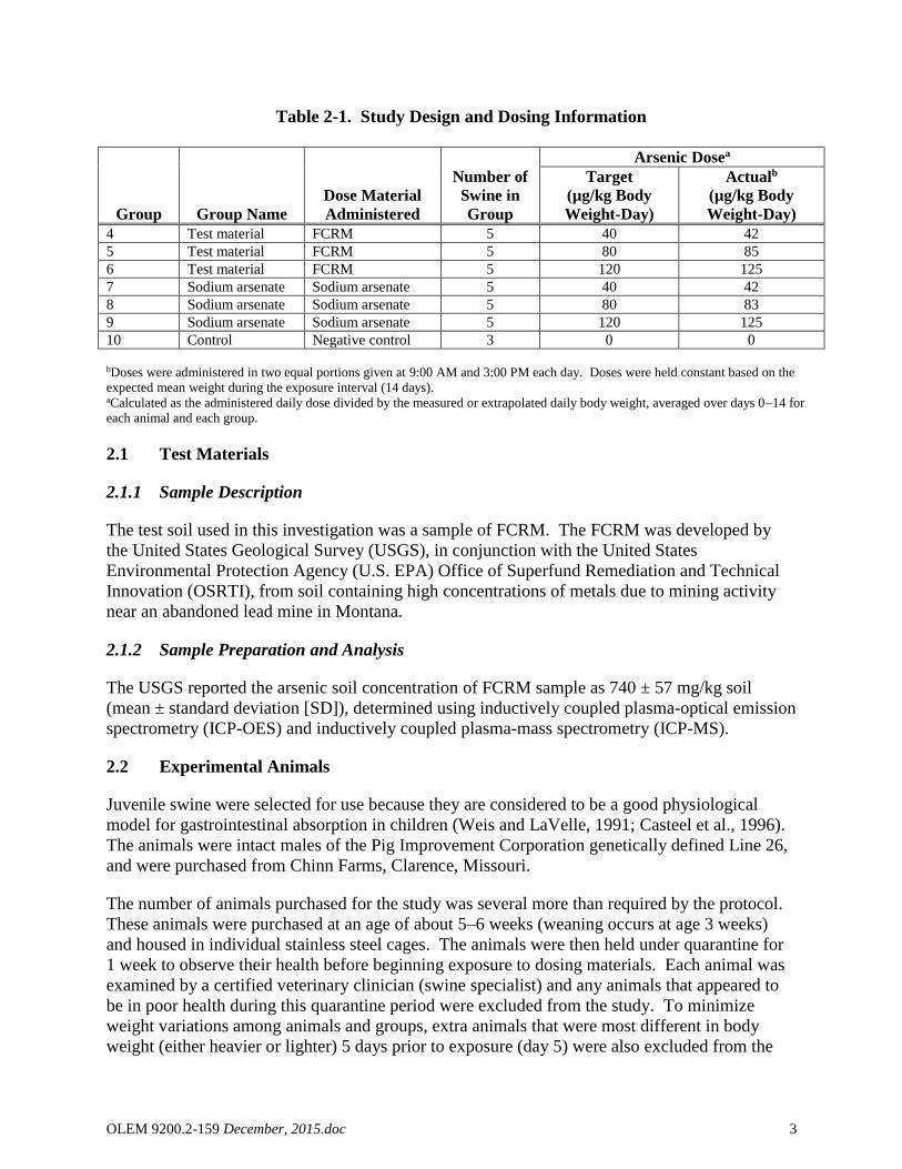
Table 2-1. Study Design and Dosing Information

Group Group Name

Dose Material

Administered

Number of

Swine in

Group

Arsenic Dosea

Target

(µg/kg Body

Weight-Day)

Actualb

(µg/kg Body

Weight-Day)

4 Test material FCRM 5 40 42



7 Sodium arsenate Sodium arsenate 5 40 42



10 Control Negative control 3 0 0

bDoses were administered in two equal portions given at 9:00 AM and 3:00 PM each day. Doses were held constant based on the

expected mean weight during the exposure interval (14 days). aCalculated as the administered daily dose divided by the measured or extrapolated daily body weight, averaged over days 0–14 for

each animal and each group.

2.1 Test Materials

2.1.1 Sample Description

The test soil used in this investigation was a sample of FCRM. The FCRM was developed by

the United States Geological Survey (USGS), in conjunction with the United States

Environmental Protection Agency (U.S. EPA) Office of Superfund Remediation and Technical

Innovation (OSRTI), from soil containing high concentrations of metals due to mining activity

near an abandoned lead mine in Montana.

2.1.2 Sample Preparation and Analysis

The USGS reported the arsenic soil concentration of FCRM sample as 740 ± 57 mg/kg soil

(mean ± standard deviation [SD]), determined using inductively coupled plasma-optical emission

spectrometry (ICP-OES) and inductively coupled plasma-mass spectrometry (ICP-MS).

2.2 Experimental Animals

Juvenile swine were selected for use because they are considered to be a good physiological

model for gastrointestinal absorption in children (Weis and LaVelle, 1991; Casteel et al., 1996).

The animals were intact males of the Pig Improvement Corporation genetically defined Line 26,

and were purchased from Chinn Farms, Clarence, Missouri.

The number of animals purchased for the study was several more than required by the protocol.

These animals were purchased at an age of about 5–6 weeks (weaning occurs at age 3 weeks)

and housed in individual stainless steel cages. The animals were then held under quarantine for

1 week to observe their health before beginning exposure to dosing materials. Each animal was

examined by a certified veterinary clinician (swine specialist) and any animals that appeared to

be in poor health during this quarantine period were excluded from the study. To minimize

weight variations among animals and groups, extra animals that were most different in body

weight (either heavier or lighter) 5 days prior to exposure (day 5) were also excluded from the


study. The remaining animals were assigned to dose groups at random (group assignments are

presented in Appendix A).

When exposure began (day 0), the animals were about 6–7 weeks old. The animals were

weighed at the beginning of the study and every 3 days during the course of the study. In each

study, the rate of weight gain was comparable in all dosing groups. Body weight data are

presented in Appendix B.

All animals were examined daily by an attending veterinarian while on study and were subjected

to detailed examination at necropsy by a certified veterinary pathologist in order to assess overall

animal health.

2.3 Diet

Animals were weaned onto standard swine chow (purchased from MFA Inc., Columbia,

Missouri) by the supplier. The feed was nutritionally complete and met all requirements of the

National Institutes of Health (NRC, 1988). The ingredients and nutritional profile of the feed are

presented in Appendix C. The measured arsenic concentration in a randomly selected feed

sample was 0.11 μg/g feed.

Beginning 5 days before the first day of dosing, each animal was given a daily amount of feed

equal to 4.0% of the mean body weight of all animals on study. Feed was reduced to 3.7% body

weight starting on day 8 of the study. Feed amounts were adjusted every 3 days, when animals

were weighed. Feed was administered in two equal portions, at 11:00 AM and 5:00 PM daily.

Drinking water was provided ad libitum via self-activated watering nozzles within each cage.

The arsenic concentration measured in six water samples from randomly selected drinking water

nozzles averaged 1.1 μg/L.

2.4 Dosing

Animals were exposed to dosing materials (sodium arsenate or test material) for 14 days, with

the dose for each day being administered in two equal portions beginning at 9:00 AM and

3:00 PM (2 hours before feeding). Swine were dosed 2 hours before feeding to ensure that they

were in a semi-fasted state. To facilitate dose administration, dosing materials were placed in a

small depression in a ball of dough consisting of moistened feed (typically about 5 g), and the

dough was pinched shut. This was then placed in the feeder at dosing time.

Target arsenic doses (expressed as µg of arsenic per kg of body weight per day) for animals in

each group were determined in the study design (see Table 2-1). The daily mass of arsenic

administered (either as sodium arsenate or as test material) to animals in each group was

calculated by multiplying the target dose (µg/kg-day) for that group by the anticipated average

weight of the animals (kg) over the course of the study:

)()/µ()/µ( kgWeightBodyAveragedaykggDosedaygMass


The average body weight expected during the course of the study was estimated by measuring

the average body weight of all animals 1 day before the study began, and then assuming an

average weight gain of 0.5 kg/day during the study. After completion of the study, the true mean

body weight was calculated using the actual body weights (measured every 3 days during the

study), and the resulting true mean body weight was used to calculate the actual dose achieved.

Any missed or late doses were recorded, and the actual doses were adjusted accordingly. Actual

doses (µg arsenic/day) for each group are shown in Table 2-1.

2.5 Collection and Preservation of Urine Samples

Samples of urine were collected from each animal for 48-hour periods on days 6–7 (U-1), 9–10

(U-2), and 12–13 (U-3) of the study. Collection began at 9:00 AM and ended 48 hours later.

The urine was collected in a plastic bucket placed beneath each cage, which was emptied into a

plastic storage bottle. Aluminum screens were placed under the cages to minimize

contamination with feces or spilled food. Due to the length of the collection period, collection

containers were emptied periodically (typically twice daily) into separate plastic bottles to ensure

that there was no loss of sample due to overflow.

At the end of each collection period, the total urine volume for each animal was measured (see

Appendix D) and three 60-mL portions were removed and acidified with 0.6 mL concentrated

nitric acid. All samples were refrigerated. Two of the aliquots were archived and one aliquot

was sent for arsenic analysis. Refrigeration was maintained until arsenic analysis.

2.6 Arsenic Analysis

Urine samples were assigned random chain-of-custody tag numbers and submitted to the

analytical laboratory for analysis in a blind fashion. The samples were analyzed for arsenic by

L.E.T., Inc. (Columbia, Missouri). In brief, 25-mL samples of urine were digested by refluxing

and then heated to dryness in the presence of magnesium nitrate and concentrated nitric acid.

Following magnesium nitrate digestion, samples were transferred to a muffle furnace and ashed

at 500°C. The digested and ashed residue was dissolved in hydrochloric acid and analyzed by

the hydride generation technique using a Perkin Elmer 3100 atomic absorption spectrometer.

This method has established that each of the different forms of arsenic that may occur in urine,

including trivalent inorganic arsenic (As+3), pentavalent inorganic arsenic (As+5), monomethyl

arsenic (MMA), and dimethyl arsenic (DMA), are all recovered with high efficiency.

Analytical results for the urine samples are presented in Appendix D.

2.7 Quality Control

A number of quality control (QC) steps were taken during this project to evaluate the accuracy of

the analytical procedures. The results for QC samples are presented in Appendix E and are

summarized below.


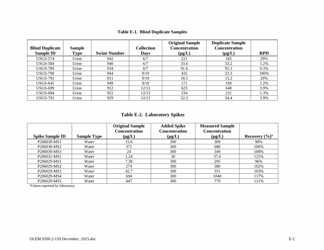
Blind Duplicates (Sample Preparation Replicates)

A random selection of about 8% of all urine samples generated during the study were prepared

for laboratory analysis in duplicate and submitted to the laboratory in a blind fashion. Results

are shown in Appendix E (see Table E-1 and Figure E-1).

Six of nine urine duplicate samples had relative percent differences (RPD) values that were <5%.

Values for the remaining three duplicates were 20, 29, and 180% (see Appendix E).

Spike Recovery

During analysis, water samples were spiked with known amounts of arsenic (sodium arsenate),

and the recovery of the added arsenic was measured. Results (see Table E-2) show that mean

arsenic concentrations recovered from spiked samples were within 10% of expected

concentrations.

Laboratory Duplicates

No duplicate urine samples were analyzed.

Laboratory Control Standards

Internal laboratory control standards were tested periodically during sample analysis. Recovery

of arsenic from these standards was generally good and within the acceptable range (see

Table E-3).

Performance Evaluation Samples

A number of Performance Evaluation (PE) samples (urine samples of known arsenic

concentration) were submitted to the laboratory in a blind fashion. The PE samples included

varying concentrations (20, 100, or 400 µg/L) each of four different types of arsenic (As+3, As+5,

MMA, and DMA). The results for the PE samples are shown in Appendix E (see Table E-4 and

Figure E-2). All sample results were close to the expected values, indicating that there was good

recovery of the arsenic in all cases.

Blanks

Laboratory blank samples were run along with each batch of samples at a rate of about 10%.

Blanks never yielded a measurable level of arsenic (all results were <1 µg/L). Results are shown

in Table E-5.

Summary of QC Results

Based on the results of all of the QC samples and the steps described above, it is concluded that

the analytical results are of sufficient quality for derivation of reliable estimates of arsenic

absorption from the test materials.


3.0 DATA ANALYSIS

3.1 Overview

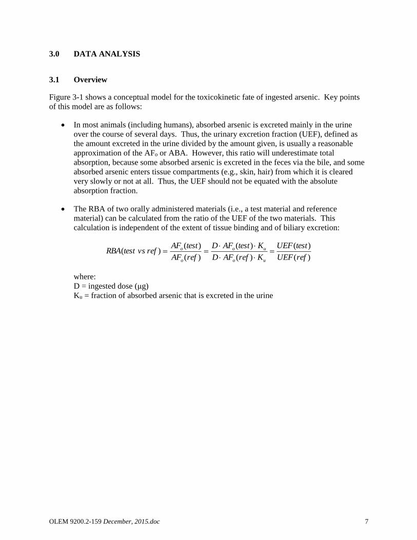
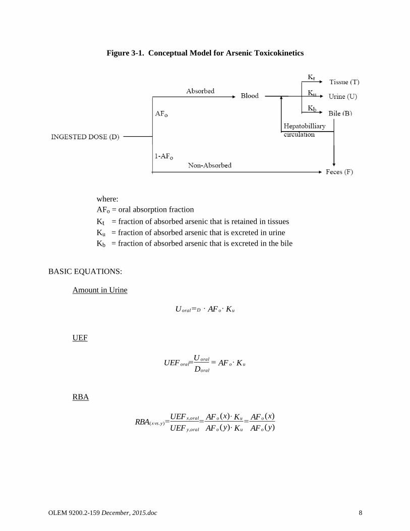
Figure 3-1 shows a conceptual model for the toxicokinetic fate of ingested arsenic. Key points

of this model are as follows:

In most animals (including humans), absorbed arsenic is excreted mainly in the urine

over the course of several days. Thus, the urinary excretion fraction (UEF), defined as

the amount excreted in the urine divided by the amount given, is usually a reasonable

approximation of the AFo or ABA. However, this ratio will underestimate total

absorption, because some absorbed arsenic is excreted in the feces via the bile, and some

absorbed arsenic enters tissue compartments (e.g., skin, hair) from which it is cleared

very slowly or not at all. Thus, the UEF should not be equated with the absolute

absorption fraction.

The RBA of two orally administered materials (i.e., a test material and reference

material) can be calculated from the ratio of the UEF of the two materials. This

calculation is independent of the extent of tissue binding and of biliary excretion:

)(

)(

)(

)(

)(

)()(

refUEF

testUEF

KrefAFD

KtestAFD

refAF

testAFrefvstestRBA

uo

uo

o

o

where:

D = ingested dose (μg)

Ku = fraction of absorbed arsenic that is excreted in the urine


Figure 3-1. Conceptual Model for Arsenic Toxicokinetics

where:

AFo = oral absorption fraction

Kt = fraction of absorbed arsenic that is retained in tissues

Ku = fraction of absorbed arsenic that is excreted in urine

Kb = fraction of absorbed arsenic that is excreted in the bile

BASIC EQUATIONS:

Amount in Urine

KAFU uoDoral

UEF

KAFD

UUEF uo

oral

oraloral

RBA

)(

)(

)(

)(

,

,).(

yAF

xAF

KyAF

KxAF

UEF

UEFRBA

o

o

uo

uo

oraly

oralxyvsx


Based on the conceptual model above, the basic method used to estimate the RBA of arsenic in a

particular test material compared to arsenic in a reference material (sodium arsenate) is as

follows:

1. Plot the amount of arsenic excreted in the urine (μg per 48 hours) as a function of the

administered amount of arsenic (μg per 48 hours) for both the reference material and the

test material.

2. Find the best fit linear regression line through each data set. The slope of each line (μg

per 48 hours excreted per μg per 48 hours ingested) is the best estimate of the UEF for

each material.

3. Calculate the RBA for each test material as the ratio of the UEF for the test material

compared to UEF for the reference material:

)(

)()(

refUEF

testUEFrefvstestRBA

3.2 Data Fitting

A detailed description of the data-fitting methods and rationale and the methods used to quantify

uncertainty in the arsenic RBA estimates for a test material are summarized below. All data

fitting was performed in Microsoft Excel® using matrix functions.

Simultaneous Regression

The techniques used to derive linear regression fits to the dose-response data are based on the

methods recommended by Finney (1978). As noted by Finney (1978), when the data to be

analyzed consist of two dose-response curves (the reference material and the test material), it is

obvious that both curves must have the same intercept, since there is no difference between the

curves when the dose is zero. This requirement is achieved by combining the two dose-response

equations into one and solving for the parameters simultaneously, as follows:

Separate Models

)()( ixbai rrr

)()( ixbai ttt

Combined Model

)()()( ixbixbai ttrr

where μ(i) indicates the expected mean response of animals exposed at dose x(i), and the

subscripts r and t refer to reference and test material, respectively. The coefficients of this


combined model are derived using multivariate regression, with the understanding that the

combined data set is restricted to cases in which one (or both) of xr and xt is zero (Finney, 1978).

Weighted Regression

Regression analysis based on ordinary least squares assumes that the variance of the responses is

independent of the dose and/or the response (Draper and Smith, 1998). It has previously been

shown that this assumption is generally not satisfied in swine-based RBA studies, where there is

a tendency toward increasing variance in response as a function of increasing dose

(heteroscedasticity) (U.S. EPA, 2007). One method for dealing with heteroscedasticity is

through the use of weighted least squares regression (Draper and Smith, 1998). In this approach,

each observation in a group of animals is assigned a weight that is inversely proportional to the

variance of the response in that group:

2

1

i

iw

where:

wi = weight assigned to all data points in dose group i

σi2 = variance of responses in animals in dose group i

When the distributions of responses at each dose level are normal, the weighted regression is

equivalent to the maximum likelihood method.

There are several alternative strategies for assigning weights. The method used in this study

estimates the value of σi2 using an “external” variance model based on an analysis of the

relationship between variance and mean response using data consolidated across many different

swine-based arsenic RBA studies. The data used to derive the variance model are shown in

Figure 3-2. As seen, log-variance increases as an approximately linear function of log-mean

response:

ln( ) ln( )s k k yi i

2 1 2

where:

si2 = observed variance of responses of animals in dose group i

yi = mean observed response of animals in dose group i

Based on these data, values of k1 and k2 were derived using ordinary least squares minimization.

The resulting values were -1.10 for k1 and 1.64 for k2.


Figure 3-2. Urinary Arsenic Variance Model

-4

1

6

11

16

0 1 2 3 4 5 6 7 8 9

ln(G

roup V

ariance)

ln(Group Mean Response)

Historical Data - Controls

Historical Data - Sodium Arsenate

Historical Data - Test Materials

Goodness of Fit

The goodness-of-fit of each dose-response model was assessed using the F test statistic and the

adjusted coefficient of multiple determinations (Adj R2) as described by Draper and Smith

(1998). A fit is considered acceptable if the p-value is <0.05.

Data Assessment

Arsenic data were assessed in two parts. First, the urine volumes and arsenic concentrations

were reviewed. A large volume of urine is typically indicative that a swine spilled its drinking

water into the urine collection trays. In these instances, the arsenic concentration in the diluted

urine will become very small and will be difficult to measure with accuracy. Furthermore,

because the response of the swine to arsenic dose is calculated from the product of urine

concentration and volume, the result becomes highly uncertain when the concentration is

multiplied by a volume that is not representative of the total urine volume. For this reason, in

cases where total urine volume per 24-hour period was >5 liters (more than twice the average

urine output of swine) and the measured urine concentration of arsenic was at or below the

quantitation limit (<2 µg/L), the samples were judged to be unreliable and were excluded from

the quantitative analysis. No samples met these criteria for exclusion.

The full dataset was modeled and analyzed for individual measured responses that appeared

atypical compared to the responses from other animals in the same dose group. Responses that


yielded standardized weighted residuals >3.5 or <-3.5 were considered to be potential outliers

(Canavos, 1984).

3.3 Calculation of RBA Estimates

The arsenic RBA values were calculated as the ratio of the slope term for the test material data

set (bt) and the reference material data set (br):

r

t

b

bRBA

The uncertainty range about the RBA ratio was calculated using Fieller’s Theorem as described

by Finney (1978).

4.0 RESULTS

4.1 Clinical Signs

The doses of arsenic administered in this study are below a level that is expected to cause

toxicological responses in swine. No clinical signs of arsenic-induced toxicity were noted in any

of the animals used in the studies. However, one swine died prior to initiating dosing. This pig

showed no signs of illness and was replaced before dosing began. Five swine received 1 cc

Naxcel once per day for several days during the study (Table 4-1) to treat a systemic bacterial

infection (swine were found with fever ≥104°F).

Table 4-1. NAXCEL Treatments

Swine Number Days of Treatment

927 -4 – -2

908 -4 – -2

944 -3 – -1

946 1–3

934 2–4

4.2 Dosing Deviations

One pig (Swine #946) missed the initial dose on day 0. This was noted during the study, but the

calculated dose amounts for days 6/7, 9/10, and 12/13 were not affected by this deviation.

4.3 Background Arsenic Excretion

Measured values for urinary arsenic excretion for control animals from days 6 to 13 are shown in

Table 4-2. Urinary arsenic concentration (mean ± SD) was 84 ± 130 µg/L (42 ± 37 µg/L after

excluding the outlier for swine 916, days 9 and 10). The values shown are generally within the

range of typical endogenous background urinary arsenic levels reported from other studies (see


Figure 3-2), although at the higher end of the detected range. This supports the view that the

animals were not exposed to any significant exogenous sources of arsenic throughout the study.

Table 4-2. Background Urinary Arsenic

Swine

Number

Urine Collection

Period

(Days)

Arsenic Dose

(µg per

Collection

Period)

Arsenic

Concentration

in Urine

(µg/L)

Urine

Volume

(mL)

Total Arsenic

Excreted

(µg/48 Hours)

911 6/7 0 32 3,520 112

940 6/7 0 34 3,400 114

916 6/7 0 37 2,520 92

911 9/10 0 19 4,085 76

940 9/10 0 21 3,340 71

916 9/10 0 419 3,300 1,383

911 12/13 0 27 4,600 124

940 12/13 0 33 3,940 130

916 12/13 0 132 1,320 174

4.4 Urinary Arsenic Variance

As discussed in Section 3.2, the urinary arsenic dose-response data are analyzed using weighted

least squares regression and the weights are assigned using an “external” variance model. To

ensure that the variance model was valid, the variance values from each of the dose groups were

superimposed on the historic data set (see Figure 4-1). As shown, aside from the control pig that

was identified as an outlier, the variance of the urinary arsenic data from this study is consistent

with the data used to generate the variance model.

4.5 Dose-Response Modeling

Urinary data for collection days 9 and 10 for control pig 916 were identified as outliers (see

Section 3.2) and were excluded from analysis. The remaining data set was analyzed (Figures 4-2

through 4-5).

All of the dose-response curves were approximately linear, with the slope of the best-fit straight

line being equal to the best estimate of the UEF. The resulting slopes (UEF estimates) for the

final fittings of the test material and corresponding reference material are shown in Table 4-3.


Figure 4-1. FCRM Data Compared to Urinary Arsenic Variance Model


Table 4-3. Urine Excretion Fraction (UEF) Estimates

Urine Collection Period (Days)

Outliers

Excluded

Slopes (UEF Estimates)

br bt

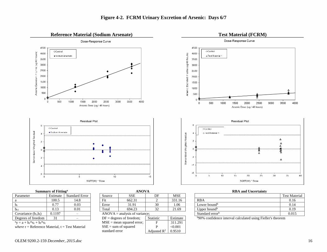
Days 6/7 0 0.77 0.13

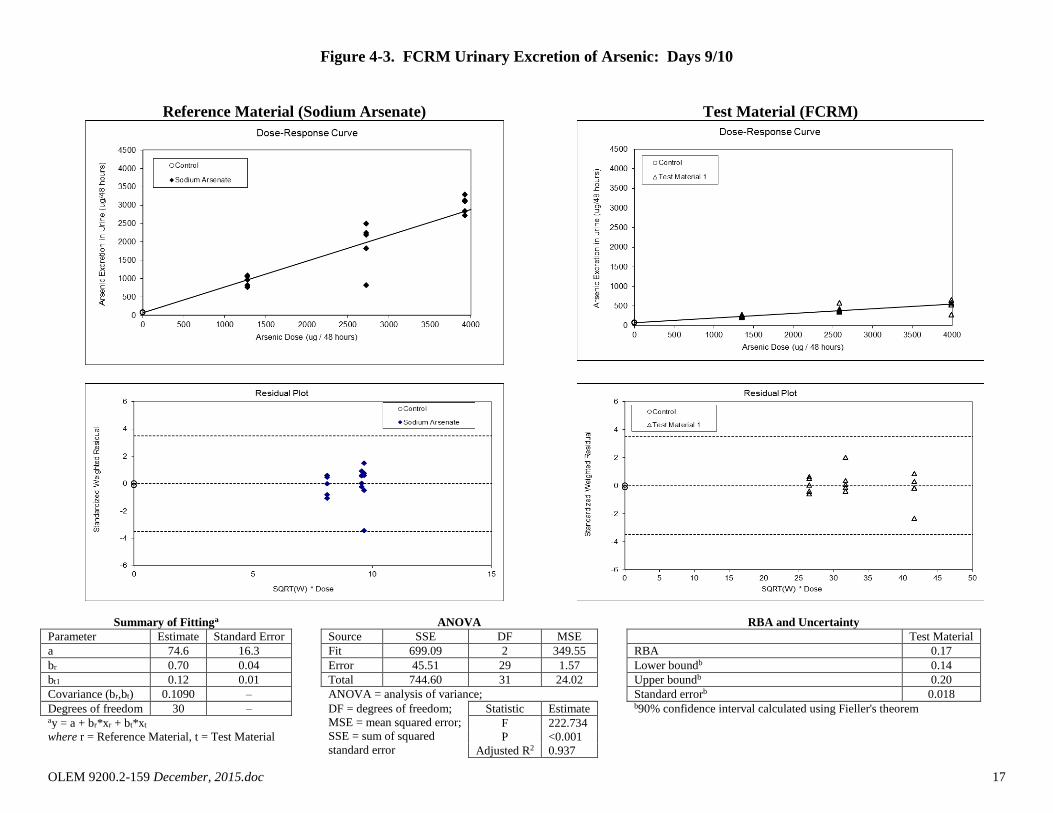
Days 9/10 1 0.70 0.04

Days 12/13 0 0.74 0.13

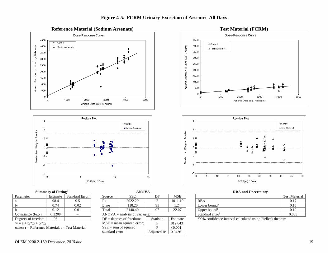
All days 0 0.74 0.12

br = slope for reference material (sodium arsenate) dose-response; bt = slope for test material 1 (FCRM) dose-response


Figure 4-2. FCRM Urinary Excretion of Arsenic: Days 6/7

Reference Material (Sodium Arsenate) Test Material (FCRM)

Summary of Fittinga

ANOVA

RBA and Uncertainty

Parameter Estimate Standard Error Source SSE DF MSE Test Material

a 100.5 14.8 Fit 662.31 2 331.16 RBA 0.16

br 0.77 0.03 Error 31.91 30 1.06 Lower boundb 0.14

bt1 0.13 0.01 Total 694.23 32 21.69 Upper boundb 0.19

Covariance (br,bt) 0.1197 – ANOVA = analysis of variance; Standard errorb 0.015

Degrees of freedom 31 – DF = degrees of freedom;

MSE = mean squared error;

SSE = sum of squared

standard error

Statistic Estimate b90% confidence interval calculated using Fieller's theorem ay = a + br*xr + bt*xt F 311.291

where r = Reference Material, t = Test Material P <0.001

Adjusted R2 0.9510




Summary of Fittinga

ANOVA

RBA and Uncertainty


a 74.6 16.3 Fit 699.09 2 349.55 RBA 0.17


bt1 0.12 0.01 Total 744.60 31 24.02 Upper boundb 0.20





standard error



Adjusted R2 0.937




Summary of Fittinga

ANOVA

RBA and Uncertainty


a 143.3 14.4 Fit 633.96 2 316.98 RBA 0.17


bt 0.13 0.01 Total 625.99 32 20.41 Upper boundb 0.19





standard error



Adjusted R2 0.9689


Figure 4-5. FCRM Urinary Excretion of Arsenic: All Days


Summary of Fittinga

ANOVA

RBA and Uncertainty


a 98.4 9.5 Fit 2022.20 2 1011.10 RBA 0.17


bt 0.12 0.01 Total 2140.40 97 22.07 Upper boundb 0.19





standard error



Adjusted R2 0.9436


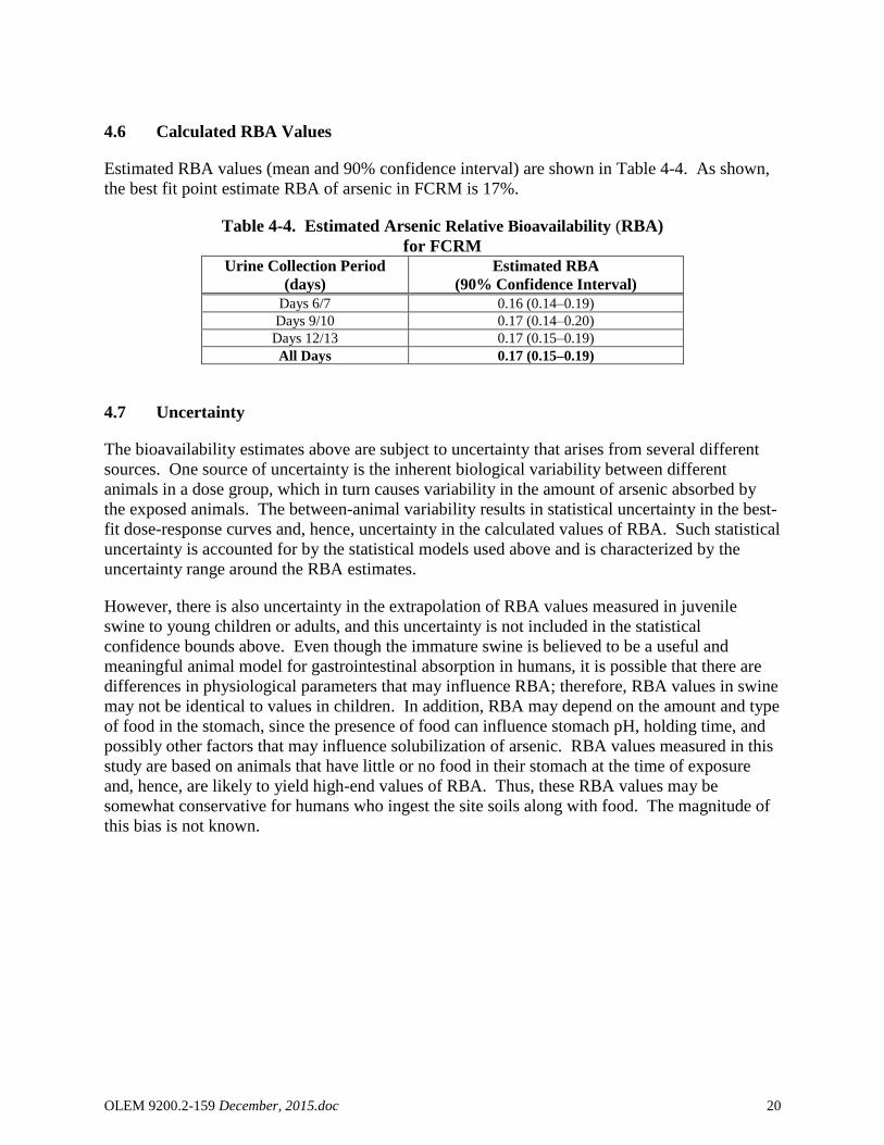
4.6 Calculated RBA Values

Estimated RBA values (mean and 90% confidence interval) are shown in Table 4-4. As shown,

the best fit point estimate RBA of arsenic in FCRM is 17%.

Table 4-4. Estimated Arsenic Relative Bioavailability (RBA)

for FCRM Urine Collection Period

(days)

Estimated RBA

(90% Confidence Interval)

Days 6/7 0.16 (0.14–0.19)

Days 9/10 0.17 (0.14–0.20)

Days 12/13 0.17 (0.15–0.19)

All Days 0.17 (0.15–0.19)

4.7 Uncertainty

The bioavailability estimates above are subject to uncertainty that arises from several different

sources. One source of uncertainty is the inherent biological variability between different

animals in a dose group, which in turn causes variability in the amount of arsenic absorbed by

the exposed animals. The between-animal variability results in statistical uncertainty in the best-

fit dose-response curves and, hence, uncertainty in the calculated values of RBA. Such statistical

uncertainty is accounted for by the statistical models used above and is characterized by the

uncertainty range around the RBA estimates.

However, there is also uncertainty in the extrapolation of RBA values measured in juvenile

swine to young children or adults, and this uncertainty is not included in the statistical

confidence bounds above. Even though the immature swine is believed to be a useful and

meaningful animal model for gastrointestinal absorption in humans, it is possible that there are

differences in physiological parameters that may influence RBA; therefore, RBA values in swine

may not be identical to values in children. In addition, RBA may depend on the amount and type

of food in the stomach, since the presence of food can influence stomach pH, holding time, and

possibly other factors that may influence solubilization of arsenic. RBA values measured in this

study are based on animals that have little or no food in their stomach at the time of exposure

and, hence, are likely to yield high-end values of RBA. Thus, these RBA values may be

somewhat conservative for humans who ingest the site soils along with food. The magnitude of

this bias is not known.


5.0 REFERENCES

Canavos, C.G. 1984. Applied Probability and Statistical Methods. Little, Brown and Co., Boston.

Casteel, S.W., Cowart, R.P., Weis, C.P., Henningsen, G.M., Hoffman, E., Brattin, W.J., Starost,

M.F., Payne, J.T., Stockham, S.L., Becker, S.V., and Turk, J.R. 1996. A swine model for

determining the bioavailability of lead from contaminated media. In: Advances in Swine in

Biomedical Research. Volume 2, Tumbleson, M.E. and Schook, L.B. (editors). Plenum Press,

New York. pp. 637–646.

Draper, N.R. and H. Smith. 1998. Applied Regression Analysis. 3rd Edition. John Wiley & Sons,

New York, NY.

Finney, D.J. 1978. Statistical Method in Biological Assay. 3rd Edition. Charles Griffin and Co.,

London.

Gibaldi, M. and Perrier, D. 1982. Pharmacokinetics. 2nd edition. Marcel Dekker, Inc, New York,

NY, pp 294–297.

Goodman, A.G., Rall, T.W., Nies, A.S., and Taylor, P. 1990. The Pharmacological Basis of

Therapeutics. 8th edition. Pergamon Press, Inc. Elmsford, NY, pp. 5–21.

Klaassen, C.D., Amdur, M.O., and Doull, J. 1996. Cassarett and Doull’s Toxicology: The Basic

Science of Poisons. McGraw-Hill, Inc. New York, NY, pp. 190.

NRC. 1988. Nutrient Requirements of Swine. A Report of the Committee on Animal Nutrition.

National Research Council. National Academy Press, Washington, DC.

U.S. EPA. 2007. Estimation of Relative Bioavailability of Lead in Soil and Soil-Like Materials

by In Vivo and In Vitro Methods. U.S. Environmental Protection Agency, Office of Solid Waste

and Emergency Response, Washington DC. OSWER 9285.7-77.

Weis, C.P. and LaVelle, J.M. 1991. Characteristics to consider when choosing an animal model

for the study of lead bioavailability. In: The proceedings of the international symposium on the

bioavailability and dietary uptake of lead. Science and Technology Letters 3:113–119.

OLEM 9200.2-159 December, 2015.doc A-1

Appendix A: Group Assignments

OLEM 9200.2-159 December, 2015.doc A-2

Table A-1. Group Assignments for FCRM Arsenic Study

Swine Number Group Treatment

Target Arsenic Dose

(µg/kg-day)

914

4 FCRM 40

948

929

952

905

906

5 FCRM 80

949

942

907

946

904

6 FCRM 120

917

934

939

924

903

7 Sodium arsenate 40

927

945

909

935

908


910

902

912

922

944


919

928

943

951

911

10 Control 0 940

916

OLEM 9200.2-159 December, 2015.doc B-1

Appendix B: Body Weights

OLEM 9200.2-159 December, 2015.doc B-2

Table B-1. Body Weights

Day -5 Day -1 Day 2 Day 5 Day 8 Day 11 Day 14

4/4/12 4/8/12 4/11/12 4/14/12 4/17/12 4/20/12 4/23/12

4 914 11.2 12.1 13.2 14 15 16 17

TM1 40 (As) 948 13.2 14 14.9 15.8 16.5 17.8 19

929 12.6 13.1 14 15.2 15.7 17 18

952 12.8 13.3 14.4 15.3 16.5 17.4 18.4

905 12.1 12.38 12.7 13.04 13.7 14.04 14.6 14.98 15.8 15.90 16.7 16.98 17.9 18.06

5 906 12.1 13.1 14 15 15.7 17.1 18

TM1 80 (As) 949 12.3 12.8 13.9 15 16 16.9 18.1

942 12 12.6 13.8 14.5 15.3 16.3 18.3

907 12.2 14.2 14.8 16 17 17.5 17.8

946 10.5 11.82 10 12.54 9.6 13.22 10.2 14.14 11.7 15.14 12.8 16.12 14.3 17.30

6 904 12.5 13.3 14.7 15.3 16.2 17 18.3

TM1 120 (As) 917 13.9 14.1 15.2 15.8 16.8 18 19.2

934 12.1 12.7 12.6 13.3 14.9 15.4 16

939 11.2 11.8 12.7 13.4 14.5 15.4 16.6

924 12.2 12.38 13 12.98 13.9 13.82 14.9 14.54 15.7 15.62 16.6 16.48 18 17.62

7 903 12.2 13.1 13 13.5 14.2 14.8 16.1

NaAs 40 927 10.2 11.3 11.8 12.5 13.6 17.3 15.5

945 13.1 13.7 14.7 15.3 16.8 17.2 18.5

909 12.5 13.2 14 14.8 16.3 14.5 18.3

935 10.1 11.62 11.1 12.48 11.8 13.06 12.8 13.78 14 14.98 14.8 15.72 16 16.88

8 908 12.3 13.2 14 14.8 15.9 16.3 17.5

NaAs 80 910 12.7 13.1 14.2 15.1 15.9 16.8 18

902 11 12.2 13 14 15.3 16.2 17.1

912 13.4 14.5 14.8 15.6 16.6 17.4 18.2

922 13.1 12.50 13.9 13.38 14.7 14.14 15.5 15.00 16.5 16.04 17.2 16.78 18.4 17.84

9 944 12.5 12.8 13.6 14.1 15 16.2 17.7

NaAs 120 919 13.4 14.4 14.9 15.3 16.6 18 18.7

928 10.7 12.1 12.8 13.6 14.6 15.5 16.4

943 11.9 12.5 13.4 13.3 14.8 16.1 18

951 10.9 11.88 11.7 12.70 12.4 13.42 13.5 13.96 15.8 15.36 15.5 16.26 18.2 17.80

10 911 11.9 12.7 13.6 14 15.1 15.8 16.6

Control 0 940 10.5 11.2 12.8 12 13.1 14.3 15

916 12.1 11.50 12.6 12.17 13.5 13.30 14.5 13.50 15.4 14.53 16.6 15.57 17.4 16.33

Weight (kg)Animal

Ear TagGroup Info Group

MBW

Group

MBW

Group

MBW

Group

MBW

Group

MBW

Group

MBW

Group

MBW

Group MBW = Mean body weight of each group.

OLEM 9200.2-159 December, 2015.doc C-1

Appendix C: Typical Feed Composition

OLEM 9200.2-159 December, 2015.doc C-2

Table C-1. Procine Grower Produced by the University of Missouri Feed Mill

Corn 1528 lbs

Bean Mill 350 lbs

Fat 50 lbs

Dicalcium phosphate 34 lbs

Limestone 18 lbs

Salt 6 lbs

Vitamins 4 lbs

Minerals 3 lbs

Zenepro 2 lbs

Biotin 2 lbs

OLEM 9200.2-159 December, 2015.doc D-1

Appendix D: Urinary Arsenic Analytical Results and

Urine Volumes for FCRM Study Samples


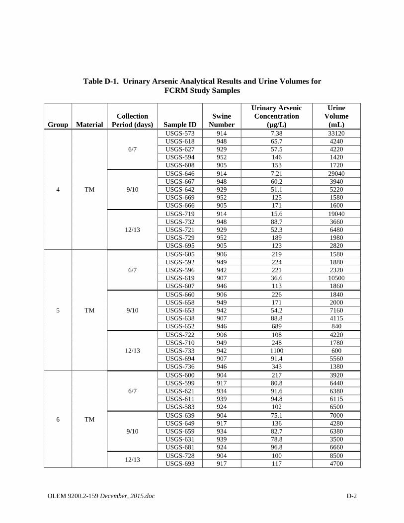
Table D-1. Urinary Arsenic Analytical Results and Urine Volumes for

FCRM Study Samples

Group Material

Collection

Period (days) Sample ID

Swine

Number

Urinary Arsenic

Concentration

(µg/L)

Urine

Volume

(mL)

4 TM

6/7

USGS-573 914 7.38 33120

USGS-618 948 65.7 4240

USGS-627 929 57.5 4220

USGS-594 952 146 1420

USGS-608 905 153 1720

9/10

USGS-646 914 7.21 29040

USGS-667 948 60.2 3940

USGS-642 929 51.1 5220

USGS-669 952 125 1580

USGS-666 905 171 1600

12/13

USGS-719 914 15.6 19040

USGS-732 948 88.7 3660

USGS-721 929 52.3 6480

USGS-729 952 189 1980

USGS-695 905 123 2820

5 TM

6/7

USGS-605 906 219 1580

USGS-592 949 224 1880

USGS-596 942 221 2320

USGS-619 907 36.6 10500

USGS-607 946 113 1860

9/10

USGS-660 906 226 1840

USGS-658 949 171 2000

USGS-653 942 54.2 7160

USGS-638 907 88.8 4115

USGS-652 946 689 840

12/13

USGS-722 906 108 4220

USGS-710 949 248 1780

USGS-733 942 1100 600

USGS-694 907 91.4 5560

USGS-736 946 343 1380

6 TM

6/7

USGS-600 904 217 3920

USGS-599 917 80.8 6440

USGS-621 934 91.6 6380

USGS-611 939 94.8 6115

USGS-583 924 102 6500

9/10

USGS-639 904 75.1 7000

USGS-649 917 136 4280

USGS-659 934 82.7 6380

USGS-631 939 78.8 3500

USGS-681 924 96.8 6660

12/13 USGS-728 904 100 8500

USGS-693 917 117 4700



FCRM Study Samples

Group Material

Collection


Swine

Number

Urinary Arsenic

Concentration

(µg/L)

Urine

Volume

(mL)

USGS-715 934 110 5920

USGS-731 939 117 4800

USGS-708 924 60.3 9860

7 Sodium

arsenate

6/7

USGS-576 903 208 3140

USGS-580 927 338 3140

USGS-597 945 133 7700

USGS-595 909 650 1940

USGS-586 935 512 2125

9/10

USGS-650 903 238 3220

USGS-663 927 375 2820

USGS-628 945 96.4 10000

USGS-680 909 305 2660

USGS-641 935 694 1560

12/13

USGS-702 903 277 3340

USGS-690 927 436 2560

USGS-724 945 112 8420

USGS-720 909 527 1980

USGS-716 935 413 2600

8 Sodium

arsenate

6/7

USGS-624 908 274 6860

USGS-612 910 1150 2110

USGS-623 902 1770 1360

USGS-622 912 628 3200

USGS-591 922 261 7320

9/10

USGS-647 908 405 2000

USGS-634 910 799 3120

USGS-635 902 1930 1160

USGS-630 912 696 3140

USGS-668 922 240 7580

12/13

USGS-697 908 371 5840

USGS-712 910 972 2600

USGS-704 902 834 3140

USGS-711 912 623 3760

USGS-707 922 234 9600

9 Sodium

arsenate

6/7

USGS-606 944 782 3640

USGS-581 919 427 6260

USGS-572 928 985 2300

USGS-616 943 697 4320

USGS-582 951 1470 2110

9/10

USGS-636 944 432 6560

USGS-656 919 475 6540

USGS-655 928 853 3180

USGS-675 943 361 8660

USGS-665 951 1690 1940

12/13

USGS-700 944 419 7080

USGS-709 919 372 8000

USGS-730 928 1320 2300



FCRM Study Samples

Group Material

Collection


Swine

Number

Urinary Arsenic

Concentration

(µg/L)

Urine

Volume

(mL)

USGS-738 943 1180 3000

USGS-734 951 2040 1860

10 Control

6/7

USGS-604 911 31.7 3520

USGS-617 940 33.6 3400

USGS-609 916 36.7 2520

9/10

USGS-651 911 18.5 4085

USGS-676 940 21.3 3340

USGS-657 916 419 3300

12/13

USGS-713 911 27 4600

USGS-698 940 33 3940

USGS-723 916 132 1320

OLEM 9200.2-159 December, 2015.doc E-1

Appendix E: Analytical Results for Quality Control

Samples


Table E-1. Blind Duplicate Samples

Blind Duplicate

Sample ID

Sample

Type Swine Number

Collection

Days

Original Sample

Concentration

(µg/L)

Duplicate Sample

Concentration

(µg/L) RPD

USGS-574 Urine 942 6/7 221 165 29%

USGS-584 Urine 940 6/7 33.6 33.2 1.2%

USGS-789 Urine 934 6/7 91.6 91.3 0.3%

USGS-790 Urine 944 9/10 432 23.3 180%

USGS-791 Urine 911 9/10 18.5 15.2 20%

USGS-645 Urine 949 9/10 171 169 1.2%

USGS-699 Urine 912 12/13 623 648 3.9%

USGS-684 Urine 922 12/13 234 231 1.3%

USGS-792 Urine 929 12/13 52.3 54.4 3.9%

Table E-2. Laboratory Spikes

Spike Sample ID Sample Type

Original Sample

Concentration

(µg/L)

Added Spike

Concentration

(µg/L)

Measured Sample

Concentration

(µg/L) Recovery (%)a

P206030-MS1 Water 15.6 300 309 98%

P206030-MS2 Water 371 300 688 106%

P206030-MS3 Water 24 300 349 108%

P206031-MS1 Water 1.24 30 37.4 121%

P206029-MS1 Water 7.38 300 295 96%

P206029-MS2 Water 274 300 580 102%

P206029-MS3 Water 42.7 300 351 103%

P206029-MS4 Water 694 300 1040 117%

P206029-MS5 Water 447 300 779 111% aValues reported by laboratory.


Table E-3. Laboratory Quality Control Standards

Sample ID

Associated

Sample Type

Measured

Concentration

(µg/L)

Detection

Limit

(µg/L) Analysis Date True Concentration Recovery (%)

P206029-BS1 Water 58.7 1 06/16/2012 60 98%

P206030-BS1 Water 59.7 1 06/16/2012 60 99%

P206031-BS1 Water 61.4 1 06/17/2012 60 102%

Table E-4. Arsenic Performance Evaluation Samples

Sample ID PE ID PE Standard

PE Concentration

(µg/L)

Sample

Concentration (µg/L)

Adjusted

Concentration (µg/L) RPD

USGS-643 as3.100 Sodium arsenite 100 151 109.3 9%

USGS-687 as3.20 Sodium arsenite 20 60.6 18.9 6%

USGS-593 As3.400 Sodium arsenite 400 498 456.3 13%

USGS-620 as5.100 Sodium arsenate 100 144 102.3 2%

USGS-662 as5.20 Sodium arsenate 20 57.1 15.4 26%

USGS-735 as5.400 Sodium arsenate 400 493 451.3 12%

USGS-737 ctrl Control urine 0 24 -17.7 -200%

USGS-625 ctrl Control urine 0 34.9 -6.8 -200%

USGS-678 dma100 Disodium methylarsenate 100 139 97.3 3%

USGS-626 dma20 Disodium methylarsenate 20 44.1 2.4 158%

USGS-691 dma400 Disodium methylarsenate 400 455 413.3 3%

USGS-706 mma100 Dimethyl arsenic acid 100 149 107.3 7%

USGS-577 mma20 Dimethyl arsenic acid 20 42.7 0.98 181%

USGS-654 mma400 Dimethyl arsenic acid 400 447 405.3 1%

PE = performance evaluation. Sample concentration adjusted by subtracting mean of background arsenic (~41.7 µg/L) from sample concentration (excluding outlier for

swine 916, days 9 and 10); RPD = relative percent difference


Table E-5. Blanks

Sample ID Associated Sample Type Measured Concentration Detection Limit Units

P206029-BLK1 Water <1 1 µg/L

P206030-BLK1 Water <1 1 µg/L

Figure E-1. Urinary Arsenic Blind Duplicates


Figure E-2. Performance Evaluation Samples

relative bioavailability of arsenic in the flat creek soil ... bioavailability of arsenic in the...

Documents