relationships of environment to composition, … of environment to composition, structure, and...
TRANSCRIPT
Relationships of Environment to Composition, Structure, and Diversity of ForestCommunities of the Central Western Cascades of OregonAuthor(s): Donald B. Zobel, Arthur McKee, Glenn M. Hawk and C. T. DyrnessSource: Ecological Monographs, Vol. 46, No. 2 (Spring, 1976), pp. 135-156Published by: Ecological Society of AmericaStable URL: http://www.jstor.org/stable/1942248 .
Accessed: 03/09/2013 16:39
Your use of the JSTOR archive indicates your acceptance of the Terms & Conditions of Use, available at .http://www.jstor.org/page/info/about/policies/terms.jsp
.JSTOR is a not-for-profit service that helps scholars, researchers, and students discover, use, and build upon a wide range ofcontent in a trusted digital archive. We use information technology and tools to increase productivity and facilitate new formsof scholarship. For more information about JSTOR, please contact [email protected].
.
Ecological Society of America is collaborating with JSTOR to digitize, preserve and extend access toEcological Monographs.
http://www.jstor.org
This content downloaded from 128.193.8.24 on Tue, 3 Sep 2013 16:39:40 PMAll use subject to JSTOR Terms and Conditions
Ecological Monographs (1976) 46: pp. 135-156
RELATIONSHIPS OF ENVIRONMENT TO COMPOSITION, STRUCTURE, AND DIVERSITY OF FOREST COMMUNITIES
OF THE CENTRAL WESTERN CASCADES OF OREGON'
DONALD B. ZOBEL, ARTHUR MCKEE, AND GLENN M. HAWK Department of Botany and Plant Pathology, Oregon State University,
Corvallis, Oregon 97331 USA AND
C. T. DYRNESS2 U.S. Forest Service, Pacific Northwest Forest and Range Experiment Station,
Corvallis, Oregon 97331 USA
Abstract. Temperature and moisture stress of conifer saplings and needle nitrogen content of conifer saplings were measured at reference stands representing 16 forest communities in the central portion of the western Cascades province of Oregon.
Most species occur over a wide range of temperature and moisture stress; many occupy a wider range of environments in the western Cascades than they do in the eastern Siskiyou Mountains of southwest Oregon. Differences between vegetation zones are reflected in a temperature index; within zones, communities are distinguished by moisture stress and, to a lesser extent, by temperature. In two cases vegetation differences appear to be related to low needle nitrogen contents. Use of complex gradients for vegetation ordination suggests certain environmental differences between communities which are contrary to the differences measured; therefore, we prefer the measured gradients over the complex gradients defined.
Species diversity (the total number of vascular species) increases and dominance (Simpson's index) decreases away from moderate environmental conditions to warmer-drier and colder communities. Diversities of different strata are unrelated. Dominance is concentrated in fewer strata of the vegetation on the colder sites. However, discontinuities in the pattern of diversity with environment occur which are not related to major differences in our measured environmental indexes. Evergreenness of shrubs is highest in stands with the lowest foliar nitrogen levels.
Key words: Coniferous forest; diversity, vegetation; moisture stress, conifers; ordination vegetation; Oregon; temperature stress, conifers.
INTRODUCTION
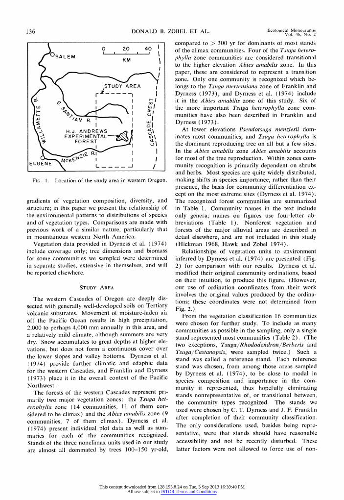
Studies of ecosystem characteristics and processes require some method of stratifying ecosystems and their subunits in all but the most homogeneous of areas. The intensity and timing of many ecosystem processes are in part determined by the type of vegetation. Because vegetation is such an important part of the ecosystem, and integrates the effect of the total environment (Billings 1952), changes in vegetation should be related to variability in many processes of interest. For these reasons a classifica- tion of forest communities was used as one of the major bases for stratifying the H. J. Andrews Ex- perimental Forest, the Oregon Intensive Study Site of the Coniferous Forest Biome, U.S. International Biological Program. This forest classification for the central portion of the Western Cascades Province (Dyrness et al. 1974) was centered on the H. J. An- drews Experimental Forest and included an area 64 X 32 km in extent (Fig. 1). Along with their forest
'Manuscript received 27 November 1974; accepted 20 June 1975.
2 Present address: Institute of Northern Forestry, Fair- banks, Alaska USA.
classification the authors included an interpretation of the major factors underlying the vegetational pat- tern. They believe that temperature differentiates vegetation zones, whereas intrazonal variation is thought to be primarily related to moisture stress.
A stratification system provided by vegetation analysis alone may not include all the information desired on environmental relationships. Plant com- munities may differ from ecosystem processes in their sensitivity to environmental factors, or they may react to factors not important to a particular process. To provide further data on the various stratification units in this area we made environ- mental measurements in selected stands representa- tive of various forest communities. These measure- ments allow a firmer decision on how appropriate the vegetation units are as stratification units. They also allow a direct gradient analysis (Whittaker 1967) of the forest vegetation of this region, where we have ob- served environmental changes along a predefined vegetation gradient. This paper reports the environ- mental measurements made, and the gradients de- fined from them. We compared measured gradients with those inferred from the vegetation and from physiographic and edaphic conditions, and with
This content downloaded from 128.193.8.24 on Tue, 3 Sep 2013 16:39:40 PMAll use subject to JSTOR Terms and Conditions
136 DONALD B. ZOBEL ET AL. Ecological Monographs Vol. 46, No. 2
0 20 40
SALEM KM
1 ~~~~~~~~~~~~~~~~~~~~ STUDY AREA
FI
Cl)
WS /4fA M R.lI
\) H.J. ANDREWS EXPERIMENTA L $ X
FOREST
EUGENE X
FiG;. 1. Location of the study area in western Oregon.
gradients of vegetation composition, diversity, and structure; in this paper we present the relationship of the environmental patterns to distributions of species and of vegetation types. Comparisons are made with previous work of a similar nature, particularly that in mountainous western North America.
Vegetation data provided in Dyrness et al. (1974) include coverage only; tree dimensions and biomass for some communities we sampled were determined in separate studies, extensive in themselves, and will be reported elsewhere.
STUDY AREA
The western Cascades of Oregon are deeply dis- sected with generally well-developed soils on Tertiary volcanic substrates. Movement of moisture-laden air off the Pacific Ocean results in high precipitation, 2,000 to perhaps 4,000 mm annually in this area, and a relatively mild climate, although summers are very dry. Snow accumulates to great depths at higher ele- vations, but does not form a continuous cover over the lower slopes and valley bottoms. Dyrness et al. ( 1974) provide further climatic and edaphic data for the western Cascades, and Franklin and Dyrness (1973) place it in the overall context of the Pacific Northwest.
The forests of the western Cascades represent pri- marily two major vegetation zones: the Tsuga het- erophylla zone (14 communities, 11 of them con- sidered to be climax) and the Abies amabilis zone (9 communities, 7 of them climax). Dyrness et al. (1974) present individual plot data as well as sum- maries for each of the communities recognized. Stands of the three nonclimax units used in our study are almost all dominated by trees 100-150 yr-old,
compared to > 300 yr for dominants of most stands of the climax communities. Four of the Tsuga hetero- phylla zone communities are considered transitional to the higher elevation Abies amabilis zone. In this paper, these are considered to represent a transition zone. Only one community is recognized which be- longs to the Tsuga mertensiana zone of Franklin and Dyrness (1973), and Dyrness et al. (1974) include it in the Abies arnabilis zone of this study. Six of the more important Tsuga heterophylla zone com- munities have also been described in Franklin and Dyrness (1973).
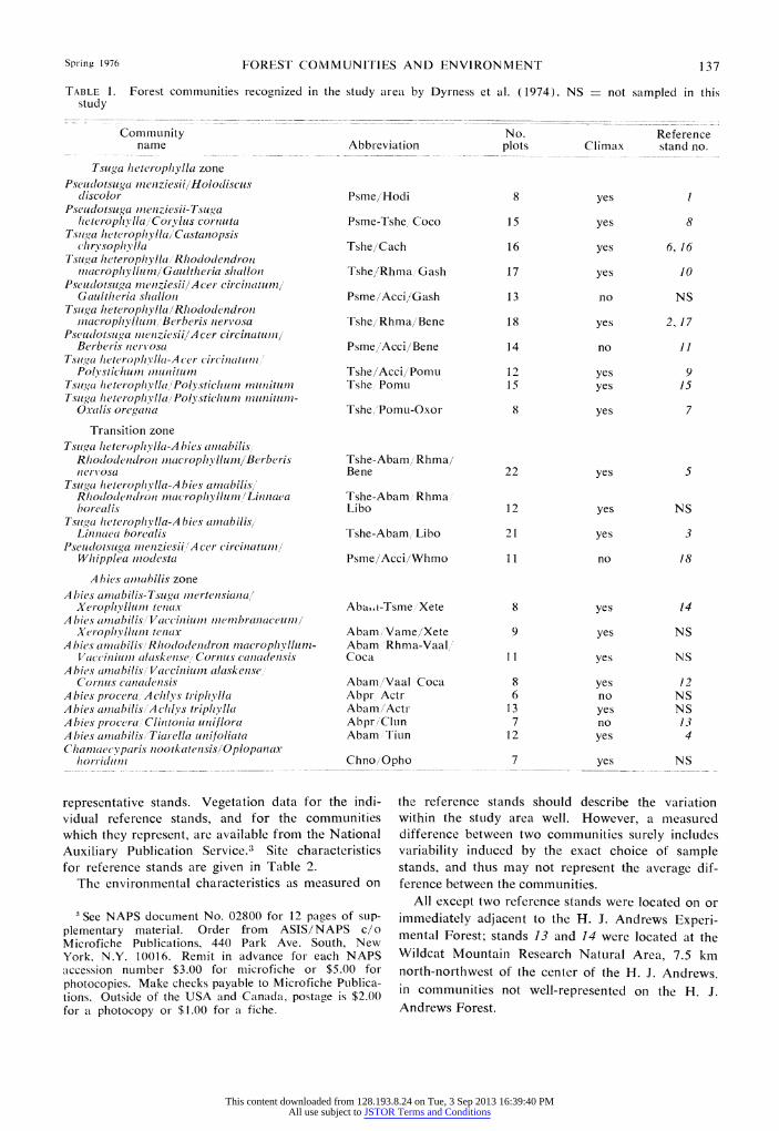
At lower elevations Pseudotsuga rnenziesii dom- inates most communities, and Tsuga heterophylla is the dominant reproducing tree on all but a few sites. In the Abies amabilis zone Abies amabilis accounts for most of the tree reproduction. Within zones com- munity recognition is primarily dependent on shrubs and herbs. Most species are quite widely distributed, making shifts in species importance, rather than their presence, the basis for community differentiation ex- cept on the most extreme sites (Dyrness et al. 1974). The recognized forest communities are summarized in Table 1. Community names in the text include only genera; names on figures use four-letter ab- breviations (Table 1). Nonforest vegetation and forests of the major alluvial areas are described in detail elsewhere, and are not included in this study (Hickman 1968, Hawk and Zobel 1974).
Relationships of vegetation units to environment inferred by Dyrness et al. (1974) are presented (Fig. 2) for comparison with our results. Dyrness et al. modified their original community ordinations, based on their intuition, to produce this figure. (However, our use of ordination coordinates from their work involves the original values produced by the ordina- tions; these coordinates were not determined from Fig. 2.)
From the vegetation classification 16 communities were chosen for further study. To include as many communities as possible in the sampling, only a single stand represented most communities (Table 2). (The two exceptions, TsugalRhododendron/Berberis and
TsugalCastanopsis, were sampled twice.) Such a stand was called a reference stand. Each reference stand was chosen, from among those areas sampled by Dyrness et al. (1974), to be close to modal in species composition and importance in the com- munity it represented, thus hopefully eliminating stands nonrepresentative of, or transitional between, the community types recognized. The stands we used were chosen by C. T. Dyrness and J. F. Franklin after completion of their community classification. The only considerations used, besides being repre- sentative, were that stands should have reasonable accessibility and not be recently disturbed. These latter factors were not allowed to force use of non-
This content downloaded from 128.193.8.24 on Tue, 3 Sep 2013 16:39:40 PMAll use subject to JSTOR Terms and Conditions
Spring 1976 FOREST COMMUNITIES AND ENVIRONMENT 137
TABLE 1. Forest communities recognized in the study area by Dyrness et al. (1974). NS - not sampled in this study
Community No. Reference name Abbreviation plots Climax stand no.
Tsuga Iietetroplhylla zone
Pseitdotsuga mnenziesii/Holodiscus discolor Psme/1Hodi 8 yes I
Pseudotsuga tnenziesii-Tsuga Iieteroplhylla Corylus cornuta Psme-Tshe/Coco 15 yes 8
Tsitga lIeteroplylla/Castanopsis chIrysophlylla Tshe/Cach 16 yes 6. 16
T'sugfa lIeteropliyllallRhIodiodienddroni mslacropliyllumljGaultheria slhallon Tshe/Rhma Gash 17 yes 10
Pseudotsuga wenziesii1A cer circinatunm Gaiult/hria sliallon Psme/Acci,'Gash 13 no NS
Tsui-a lieteropllylla RIhotlodlendron muacroplyllium,;Berberis neri'osa Tshe/Rhma/'Bene 18 yes 2, 17
Pseudotsuga nienziesii/A cer circinatuuin Berberis nerv'osa Psme/'Acci/Bene 14 no 11
Tsugai hIeterophlvyll(-A(er circinatuiml,. Polixstichumn inuniturn Tshe/Acci//'Pomu 12 yes 9
Tsuga lieteroplivllai'Polysticliuiii muinitunm Tshe Pomu 1 5 yes 15 Tsiiga Ilhterophllala/ Polysticlhunm munitumi-
Oxalis oregana Tshe/ Pomu-Oxor 8 yes 7
Transition zone Tsuga Iheteir-pylla-A bies alilabilis
Rhododendron fIlacrophl lluml/Ber beris Tshe-Abam/ Rhma/ ierivosa Bene 22 yes 5
Tsuga lieterophylla-A bies ainabilis, Rhododendron tniaMC'ropliyl/luinLiiiiia(ea Tshe-Abam RRhma' bworealis Libo 12 yes NS
Tsugra Iwterophylla-A bies aniabilis, Linnaea borealis Tshe-Abam,'Libo 21 yes 3
Pseudotsuga tnenziwsiijA ceri- (rili-lbatulnl/ Whipplea muodesta Psme/Acci/Whmo 11 no 18
Abies amabilis zone A bies aniabilis- Tsuga inertensiana
Xerophyllu'n tenax Aba ia-Tsme Xete 8 yes 14 A bies anlabilis,/" Vaccinium iniemflbraiiaceuml/
Xero'hplilmyl/ tuelax Abam, IVame/Xete 9 yes NS A bies amnabilisR1 Rhododendron mnacrophylliumn- Abam Rhmna-Vaal,'
V'accillium alaskn use; Cornius canadensis Coca 11 yes NS A bies anlabilis ,Vacciilum alaSkeuiSe
Cornuss calanadelsis Abam 'Vaal Coca 8 yes 12 Abies procura AdAchlys triphylla Abpr Actr 6 no NS Abies ainabilis/A chlys triphylla Abam/Actr 13 yes NS Abies procuua,/Clintonia uniflora Abpr/Clun 7 no 13 A bies amnabilis Tiairella unifoliata Abam iTiun 12 yes 4 Chamaecyparis nootk atensis,/Oplopanax
Iio, r idlu~s iChno/Opho 7 yes NS
representative stands. Vegetation data for the indi- vidual reference stands, and for the communities which they represent, are available from the National Auxiliary Publication Service.3 Site characteristics for reference stands are given in Table 2.
The environmental characteristics as measured on
'See NAPS document No. 02800 for 12 pages of sup- plementary material. Order from ASIS/NAPS c/o Microfiche Publications, 440 Park Ave. South, New York. N.Y. 10016. Remit in advance for each NAPS accession number $3.00 for microfiche or $5.00 for photocopies. Make checks payable to Microfiche Publica- tions. Outside of the USA and Canada, postage is $2.00 for a photocopy or $1.00 for a fiche.
the reference stands should describe the variation within the study area well. However, a measured difference between two communities surely includes variability induced by the exact choice of sample stands, and thus may not represent the average dif- ference between the communities.
All except two reference stands were located on or immediately adjacent to the H. J. Andrews Experi- mental Forest; stands 13 and 14 were located at the Wildcat Mountain Research Natural Area, 7.5 km north-northwest of the center of the H. J. Andrews, in communities not well-represented on the H. J. Andrews Forest.
This content downloaded from 128.193.8.24 on Tue, 3 Sep 2013 16:39:40 PMAll use subject to JSTOR Terms and Conditions

138 DONALD B. ZOBEL ET AL. Ecological Monographs Vol. 46, No. 2
HOT .40 gPsme/
Tshei Psrne- f/cd!'
T~~~~~~~~~~~~~~~~~~~ci 6 C3 x 8 ? Ts/,e/ ~ ~ ~ ~ ~ Cah Tse
Tshe ~~~Rhmnci l | ~~~~~~~ ~~~Rhmcl Gash 1 0
Tshe/ gene 2 -- TSUGA HETEROPHYLLA Accll ,# D_ -
Tshe/ Ts/,e' Pcrm Prnei1 PS/7W/
ZONE PoIu- II L . . . J Accil ui Oxcr 7 Pcu4c/ 'Gs
-
X ~~~~~~~~~~~R/mc/Bene
Cie TshelTshe- AbPm e 7se-C TRANSITION ZONE
Z ~~~~~~~L/bc W3 jlsbeAw .1Litc
LU Acc/ / I
AbX'r ABIES AMABILIS IAbor.' Abprl C/un7 L31 i Acfr IN ZONE
Tlun 4 Ai Vaern/ Chnc/ el Abem-
Ophc Tsme LI COLIL
MOIST DECREASING MOISTURE --)DR Y
FIG. 2. Hypothesized relationships between forest communities and environment in the central western Cascades (Dyrness et al. 1974: Fig. 5). This figure is based on their vegetation ordination, somewhat modified by the intu- ition of the investigators. Communities enclosed with dashed borders are considered to be sera], the others, to be climax. Communities sampled in this study are identified by the reference stand number in the box. Abbreviations for commUnities are identified in Table 1.
MEASUREMENT OF ENVIRONMENTAL INDEXES
Methods
The environmental measurements we made were related to small conifer saplings in order to quantify the environment as integrated by trees of this size. In- dexes of moisture and mineral nutrient availability were determined by direct measurements of plant moisture stress and needle nutrient content, respec- tively. Air and soil temperature were measured for major strata occupied by foliage and roots of these understory trees. The length of the summary season for the temperature index was partially determined by sapling phenology.
Temperature was measured continuously at one site in each reference stand, using a two-pen 30-day thermograph. Air temperature was taken at 1 m under an insulated A-frame shield which shaded the probe. The soil temperature probe was buried nearby at a depth of 20 cm. Air temperatures were digitized and each daily maximum, minimum, and mean was computed. Separate means were computed for day-
light and night. Daylength for the 15th of each month was used to determine the day and night summation periods. Average daily soil temperatures were read from the charts manually. Monthly means, seasonal extremes, and other data were determined as needed.
In August 1973 soil temperature at 20 cm was measured at 11 points in each stand in order to assess how representative the sampling point was. One measurement was at the site of the thermograph probe, the others at the base of 1-3-m conifer sap- lings. Means for each stand were computed and compared with the measurement at the thermograph probe.
A temperature summing formula was used which weights temperatures by their effect on production of seedlings of Pseudotsuga menziesii in controlled en- vironments (Cleary and Waring 1969). This cal- culates an index originally called "Optimum Temperature Days" which has been renamed Temperature Growth Index (TGI) by its originators. Average soil and daylight air temperature were used to compute the index for each day, and the daily
This content downloaded from 128.193.8.24 on Tue, 3 Sep 2013 16:39:40 PMAll use subject to JSTOR Terms and Conditions
Spring 1976 FOREST COMMUNITIES AND ENVIRONMENT 139
TABLE 2. Characteristics of reference stands sampled. Percent cover is for a 50 X 50-rn area at each stand. Specific names of plants in the community names are given in Table I
Percent cover Refer- Tree ence Eleva- stand tion As- Slope Ma- Repro-
Zone no. Community (i) pect (0) ture dLucing Shrub Herb
Tsuga heteropitylla I Pseudotsuga 'Holodiscus 510 SW 35 50 20 46 36 2 Tsuga, 'RhododendronlBerberis 520 NW 20 105 10 30 24 6 Tsuga, Castantiopsis 710 S 40 83 30 123 14 7 T'suga/lPolystichum-Oxalis 490 NW 18 110 42 17 41 8 Plseudotsuga-Tsuga/Corylus 500 W 40 81 25 64 27 9 Tsuga,/A cer,/Polystichum 490 WNW 45 100 35 72 48
10 Tsuga/Rhododendron/l Gaultlheria 670 SSW 5 89 60 118 7
II PseudotsugajlAcer/Berherisv 1,060 SSE 25 96 35 62 10 15 Tsug~a 'Polystichum 720 NW 45 108 43 14 18 16 Tsug~a/Castanopsis 670 SW 40 107 48 108 7 17 Tsu ga/Rhododendron!
Berberis 530 NNW 18 102 47 43 37
Transition 3 Tsuga-A bies/Liniiaea 950 SW 10 120 88 38 24 5 Tsu ga-A b ies/Rhododendron/
Berberis 920 N 8 90 27 125 5 18 Pseudotsuga,/A cer /' Wh ipplea 1,080 SE 30 81 24 92 23
Abies amzabilis 4 Abies/Tiarella 1,440 SW 10 116 50 9 39 12 A biesi/Vacciniuni/Cornus 1,020 W 5 103 31 56 33 13 A bies/'Clintonia 1,480 S, 15 93 20 12 3 2 14 A bies-Tsiuga,"1Xerophyllum_ 1,570 NW 15 100 27 3 33
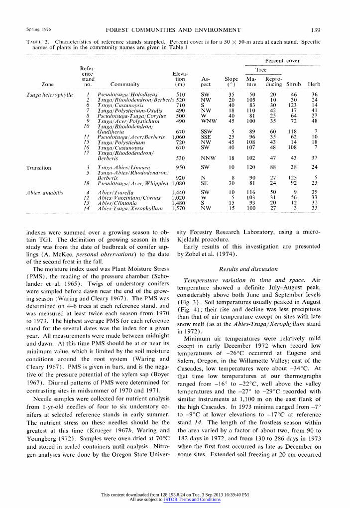
indexes were summed over a growing season to ob- tain TGI. The definition of growing season in this study was from the date of budbreak of conifer sap- lings (A. McKee, personal observations) to the date of the second frost in the fall.
The moisture index used was Plant Moisture Stress (PMS), the reading of the pressure chamber (Scho- lander et al. 1965). Twigs of understory conifers were sampled before dawn near the end of the grow- ing season (Waring and Cleary 1967). The PMS was determined on 4-6 trees at each reference stand, and was measured at least twice each season from 1970 to 1973. The highest average PMS for each reference stand for the several dates was the index for a given year. All measurements were made between midnight and dawn. At this time PMS should be at or near its minimum value, which is limited by the soil moisture conditions around the root system (Waring and Cleary 1967). PMS is given in bars, and is the nega- tive of the pressure potential of the xylem sap (Boyer 1967). Diurnal patterns of PMS were determined for contrasting sites in midsummer of 1970 and 1971.
Needle samples were collected for nutrient analysis from 1-yr-old needles of four to six understory co- nifers at selected reference stands in early summer. The nutrient stress on these needles should be the greatest at this time (Krueger 1967b, Waring and Youngberg 1972). Samples were oven-dried at 70'C and stored in scaled containers until analysis. Nitro- gen analyses were done by the Oregon State Univer-
sity Forestry Research Laboratory, using a micro- Kjeldahl procedure.
Early results of this investigation are presented by Zobel et al. (1974).
Results and discussion
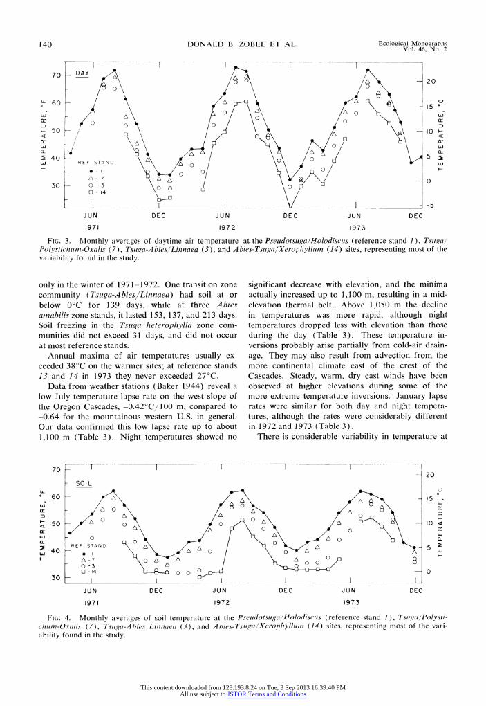
Temperature variation in time and space. Air temperature showed a definite July-August peak, considerably above both June and September levels (Fig. 3). Soil temperatures usually peaked in August (Fig. 4); their rise and decline was less precipitous than that of air temperature except on sites with late snow melt (as at the Abies-Tsuga/Xerophyllurn stand in 1972).
Minimum air temperatures were relatively mild except in early December 1972 when record low temperatures of -260C occurred at Eugene and Salem, Oregon, in the Willamette Valley; east of the Cascades, low temperatures were about -340C. At that time low temperatures at our thermographs ranged from -16? to -220C, well above the valley temperatures and the -27? to -290C recorded with similar instruments at 1,100 m on the east flank of the high Cascades. In 1973 minima ranged from -7? to -90C at lower elevations to -17'C at reference stand 14. The length of the frostless season within the area varied by a factor of about two, from 90 to 182 days in 1972, and from 130 to 286 days in 1973 when the first frost occurred as late as December on some sites. Extended soil freezing at 20 cm occurred
This content downloaded from 128.193.8.24 on Tue, 3 Sep 2013 16:39:40 PMAll use subject to JSTOR Terms and Conditions
140 DONALD B. ZOBEL ET AL. Ecological Monographs Vol. 46, No. 2
- I I - F -~~~~~~~~~~~~~~~~~~~ _ _ _ _ _ __~~~~--- -- - - - -
70 DAY A
A ~~~20
60 U~0
15
o 0 ~~~~~~~~~00 0 0 D~~~~~~~~~
H-50- < ~ ~ ~ ~ ~ ~ ~ ~ ~ ~ ~ ~ ~ ~~~A10H
Lu 0 U
iuJ REF STAND A 0
7-0- H
30 0-3 0 0 0 0 1 4
-5
JUN DEC JUN DEC JUN DEC
1971 197 2 197 3
FIG. 3. Monthly averages of daytime air temperature at the Pseudotsuga/Holodiscus (reference stand 1), Tsugal Polysticlhuni-Oxalis (7), Tsuga-Abies'Linnaea (3), and Abies-Tsuga/Xeroplhyllutn (14) sites, representing most of the variability found in the study.
only in the winter of 1971-1972. One transition zone community (Tsuga-AbieslLinnaea) had soil at or below 0C for 139 days, while at three Abies arnabilis zone stands, it lasted 153, 137, and 213 days. Soil freezing in the Tsuga heterophylla zone com- munities did not exceed 31 days, and did not occur at most reference stands.
Annual maxima of air temperatures usually ex- ceeded 380C on the warmer sites; at reference stands 13 and 14 in 1973 they never exceeded 270C.
Data from weather stations (Baker 1944) reveal a low July temperature lapse rate on the west slope of the Oregon Cascades, -0.420C/100 m, compared to -0.64 for the mountainous western U.S. in general. Our data confirmed this low lapse rate up to about 1,100 m (Table 3). Night temperatures showed no
significant decrease with elevation, and the minima actually increased up to 1,100 m, resulting in a mid- elevation thermal belt. Above 1,050 m the decline in temperatures was more rapid, although night temperatures dropped less with elevation than those during the day (Table 3). These temperature in- versions probably arise partially from cold-air drain- age. They may also result from advection from the more continental climate east of the crest of the Cascades. Steady, warm, dry east winds have been observed at higher elevations during some of the more extreme temperature inversions. January lapse rates were similar for both day and night tempera- tures, although the rates were considerably different in 1972 and 1973 (Table 3).
There is considerable variability in temperature at
70 - - - 2 0 _20 SOIL
197 1 15 1 Lii0 cr_ cr_0D
< 0 ~~~~~~~~~~~~~~~~~~~~~~~~~~~~~~0cr_ cr_ 0 Uj~~~~~~~~~~~~~~~~~~~~~~~~~~~~~~~~~~~~~~~~~c
Q- 0 0~~~~~~~~~~~~~~~~~~~~~~~~
30-
J UN DEC J UN DEC J UN DEC
1971 1972 197 3
FIG. 4. Monthly averages of soil temperature at the Pseudotsugal/Holodiscus (reference stand 1), TsugaljPolvsti- chitm-O-valis (7), Tsuga-Ahies Limiiuaea (3), and Abhies-Tsuga/Xerophyllum (14) sites, representing most of the vari- ability found in the study.
This content downloaded from 128.193.8.24 on Tue, 3 Sep 2013 16:39:40 PMAll use subject to JSTOR Terms and Conditions

Spring 1976 FOREST COMMUNITIES AND ENVIRONMENT 141
TABLE 3. Temperature changes (?C,"100 m) with elevation on the study area. Two sites at lower elevations, ad- jacent to the H. J. Andrews Forest, are included in the data. Significant correlation of temperature with elevation at 0.05 and 0.01 levels are designated by the symbols * and **, respectively
July January
Below 1, 1 00 m Above 1,050 m Below 1,100 m
1971 1972 1973 1972 1973 1972 1973
No. samples 11 16 16 5 6 9 17
Mean day -0.26 -0.33** -0.28* -0.80* -0.71* -0.43 * -0.24* Mean night -0.09 -0.09 -0.17 -0.46 -0.40 -0.37** -0.1 8 *
Mean max -0.38* -0.54** -0.54** -1.13* -0.98** -0.46* -0.22* Mean min +0.16 +0.18 +0.06 -0.47 -0.21 -0.28** -0.24** Mean range -0.54** -0.73** -0.61** -0.65* -0.79* -0.18 +0.02 Mean soil -0.28 -0.47** -0.37 -0.67 -0.43 -0.34* -0.21**
a given elevation. For example, the seven stands with elevations A 500 m had the following temperature ranges in July 1972: absolute minimum, 3-80C; absolute maximum, 31-40'C; and daytime mean, 19-230C.
Baker (1944) also noted a 180C diurnal tempera- ture variation in July for our region, which he said changed little with elevation. Our summer diurnal range approached this figure only at low elevations, and it declined 0.540C or more per 100 m over all elevations (Table 3). Winter diurnal range was about 3-60C; it showed little change with elevation (Table 3).
Variability within stands could lead to serious anomalies in our data if the sampling point were not representative. However, soil temperatures measured throughout the stand generally compared fairly well with those measured at the probe. On only 5 of the 18 reference stands did soil temperature at the probe site in August 1973 differ by more than 1.00C from the mean of 11 points in the stand, and all were within 20C of the mean. Means for the stand were almost always lower than the temperature at the probe. Correlation between soil temperature at the thermograoh site and stand soil temperature mean was r = 0.94.
Values for stands within the same vegetation type would also be expected to vary. We replicated only two communities, Tsuga/Rhododendron/Berberis, and Tsuga/Castanopsis, each at two sites (Table 1). Monthly averages of air and soil temperatures varied up to 2.20C between replicate stands of the same community (Table 4). The temperature relationship reversed itself with season in most cases. For ex- ample, in April stand 2 was 1.1 C cooler than stand 17; in October it was 1.70C warmer. The pattern of difference between replicate reference stands was not the same for soil temperature as for air temperature with stands 6 and 16; between stands 2 and 17 soil and air temperature varied in a parallel fashion.
Temperature growth index. Temperature growth index (TGI) at the reference stands varied consider- ably during 1971 to 1973 (Table 5). In 1973 the index was higher than for the other 2 yr, especially at the cooler sites, due to unusually late fall frosts. However, the relative positions of communities were similar from year to year. Correlation analysis of TGI of individual stands in 1971 with that in 1972 gave a coefficient of determination (r2) of 0.98 (n -
12); the comparison of 1972 TGI with TGI in 1973 had r2 = 0.96 (n - 14).
Communities sampled in the different vegetation zones are clearly separated by TGI in all 3 yr (Table 5). However, variability in TGI does not correspond particularly well with vegetational changes within the Tsuga heterophylla and transition zones (Fig. 5). A major cause of the poor relationship between TGI and the Y-axis coordinate is the position of reference stands 6 and 10; for the other stands, TGI generally decreases as the Y-coordinate increases, with a similar pattern repeated for the 3 yr represented in Fig. 5. A possible cause for the failure of stands 6 and 10 to conform to the general relationship is presented in th- section on foliar nutrition.
Use of TGI accentuates the differences among sites seen in unweighted temperature data. There is rela-
TABLE 4. Differences between monthly means of day air temperature and soil temperature in replicate refer- ence stands representing the same community. Data are for July 1972 through December 1973. Stands 2 and 17 represent the Tsuga/Rhododendron/Berberis community; stands 6 and 16 represent the Tsuga/ Castanopsis community
Day air temperature Soil temperature _(0C) (OC)
Reference stand (2-17) (6-16) (2-77) (6-16)
Mean difference ?0.41 ?0.91 ?0.58 -0.23
Range of monthly -1.9 to -0.1 to -1.3 to -1.6 to differences ?1.9 ?2.2 +1.7 ?0.9
This content downloaded from 128.193.8.24 on Tue, 3 Sep 2013 16:39:40 PMAll use subject to JSTOR Terms and Conditions

142 DONALD B. ZOBEL ET AL. Ecological Monographs Vol. 46, No. 2
x loo a a z 0
A 0
r 0~~~~~~ H A
0 0a
cr_ ?0 0 0~~~~~~ I
0
cr_ ~~~~~~~0 0
60 0 = 1971 - Lii 0 =19720
Q_ an = 1973 A2I730
LIJ
9 REF STAND NO. 6 10 8 1 2 1157 3
40 I ! I 0 20 40 60
Y- AXIS COORDINATE
FIG. 5. Relationship of Temperature Growth Index of reference stands and the y-axis coordinate of the com- munity the stands represent in a vegetation ordination, for Tsuga lieterophylla zone and transitional communities. Communities represented by the reference stands are identified in Table 2.
tively more variation within elevational zones and the overall rate of decline with increasing elevation is considerably greater than any lapse rate for mean temperature. Although TGI is significantly correlated with plot elevation (r2 - 0.74, 0.86, and 0.84 for
1971, 1972, and 1973), there is considerable vari- ability within elevational zones, enough to justify use of a temperature index other than elevation itself. For example, vegetation at reference stand 12 at 1,020 m placed it in the Abies amabilis zone, whereas stand 11 at 1,060 m was in the Tsuga heterophylla zone. The TGI values conform to the zone deter- mined by the vegetation and do not overlap (Table 5).
The large change in TGI from the transition to the Abies amabilis zone stands appears to be due partially to the steeper lapse rate at higher elevations, as well as possibly to sampling idiosyncracies. Another large environmental change seems to occur below the highest elevation stand in the study. The Abies- Tsuga/Xerophylluin community there would be placed into the Tsuga inertensiana zone in a regional context (Franklin and Dyrness 1973). This site often has the deepest snowpack and has the coldest soil of any of our sample sites. This situation may be analogous to southern British Columbia where snow accumulation increases and species composition changes abruptly above a certain elevation, with the loss of Tsuga heterophylla and Pseudotsuga menziesii (Brooke et al. 1970); this same shift in tree composition occurs from our Abies/Clintonia to thb Abies-TsugalXerophylluin stand.
At the replicate stands of the TsugalCastanopsis community (stands 6 and 16), the 1973 TGI differed only by 1 unit, despite the relatively larger differences in air and soil temperature means (Table 4). How-
TFABLE 5. Temperature growth index (TGI) for reference stands in 1971 to 1973
Reference TGI stand Plant _ -
Vegetation zone no. community 1971 1972 1973
Tsuga heterophylla I PseudlotsugalHolodiscus 95 102 107 2 TsugalRhIododendronlBer-beris 74 84 99 6 Tsuga/ Castanopsis 85 93 92 7 TsugalPolysticlium-Oxalis 80 82 88 8 Pseudotsuga-Tsuga/Corylus 90 98 101 9 TsugalA cer/Polystichunm 81 87 98
10 TsugaIRliododlendlr-on/Gaultlheu ia 76 83 91 11 Pseudotsuga/A cer/Berberis 73 78 92 15 Tsuga/Polysticeum 89 16 Tsuga/Castanopsis 93 17 TsugalRliododendron/Berberis 88
Zone average 82 88 94
Transition 3 Tsuga-A bies Linnaea 56 67 77 5 Tsuga-A bies/Rhlododendr onlBerber is 60 70 82
Zone average 58 69 80
Abies aniabilis 4 Abies/Tiarella 34 38 52 12 Abies/'Vaccin imn/Cornus 40 49 68 13 AbieslClintonia 37 52 14 A bies-TsugalXerophylluin 32 53
Zone average 36 39 56
This content downloaded from 128.193.8.24 on Tue, 3 Sep 2013 16:39:40 PMAll use subject to JSTOR Terms and Conditions
Spring 1976 FOREST COMMUNITIES AND ENVIRONMENT 143
ever, the replicates of TsugalRhododendron/Berberis (stands 2 and 17) had a TGI difference of 11 units. Much of this difference is attributable to a local late occurrence of fall frost at stand 2, allowing it 28 more days during which TGI units were accumulated.
Plant moisture stress. Rainfall during the four summers in which plant moisture stress was measured varied considerably. Summers of 1970 and 1972 were quite dry, leading to similarly high PMS levels late in the season. 1971 was relatively wet, with no dry spell longer than 3 wk. In 1973, although there was little precipitation and very low streamflows, there were only intermediate levels of moisture stress.
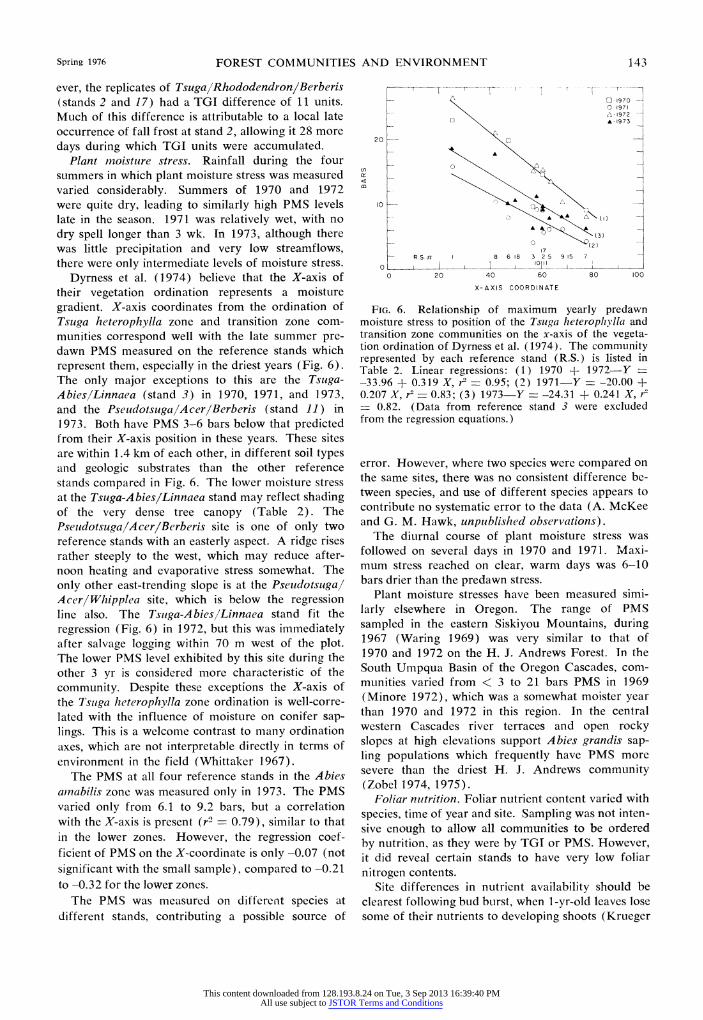
Dyrness et al. (1974) believe that the X-axis of their vegetation ordination represents a moisture gradient. X-axis coordinates from the ordination of Tsuga heterophylla zone and transition zone com- munities correspond well with the late summer pre- dawn PMS measured on the reference stands which represent them, especially in the driest years (Fig. 6). The only major exceptions to this are the Tsuga- Abies/Linnaea (stand 3) in 1970, 1971, and 1973, and the PseudotsugalAcer/Berberis (stand 11) in 1973. Both have PMS 3-6 bars below that predicted from their X-axis position in these years. These sites are within 1.4 km of each other, in different soil types and geologic substrates than the other reference stands compared in Fig. 6. The lower moisture stress at the Tsuga-Abies/Linnaea stand may reflect shading of the very dense tree canopy (Table 2). The Pseudotsuga/Acer/Berberis site is one of only two reference stands with an easterly aspect. A ridge rises rather steeply to the west, which may reduce after- noon heating and evaporative stress somewhat. The only other east-trending slope is at the Pseudotsugal AcerlWhipplea site, which is below the regression line also. The Tsuga-A bies/Linnaea stand fit the regression (Fig. 6) in 1972, but this was immediately after salvage logging within 70 m west of the plot. The lower PMS level exhibited by this site during the other 3 yr is considered more characteristic of the community. Despite these exceptions the X-axis of the Tsuga heterophylla zone ordination is well-corre- lated with the influence of moisture on conifer sap- lings. This is a welcome contrast to many ordination axes, which are not interpretable directly in terms of environment in the field (Whittaker 1967).
The PMS at all four reference stands in the Abies ainabilis zone was measured only in 1973. The PMS varied only from 6.1 to 9.2 bars, but a correlation with the X-axis is present (r2 - 0.79), similar to that in the lower zones. However, the regression coef- ficient of PMS on the X-coordinate is only -0.07 (not significant with the small sample), compared to -0.21 to -0.32 for the lower zones.
The PMS was measured on different species at different stands, contributing a possible source of
T T A -E r r - T- --
l-D1970 \ -1971
Ad- 1972 A - 1973
20
(2 ~~~~~~~~~~A
10
- Alto >~~~~ (3) -
__ 0 (2) 17
RS.# 1 8 6 18 3 25 9 15 7
O 10 I 1
0 20 40 60 80 100
X-AXIS COORDINATE
FIG. 6. Relationship of maximum yearly predawn moisture stress to position of the Tsuga heteroplhylla and transition zone communities on the x-axis of the vegeta- tion ordination of Dyrness et al. (1974). The community represented by each reference stand (R.S.) is listed in Table 2. Linear regressions: (1) 1970 + 1972-Y = -33.96 + 0.319 X, r2 - 0.95; (2) 1971-Y = -20.00 + 0.207 X, r2 - 0.83; (3) 1973-Y --24.31 + 0.241 X, r2 = 0.82. (Data from reference stand 3 were excluded from the regression equations.)
error. However, where two species were compared on the same sites, there was no consistent difference be- tween species, and use of different species appears to contribute no systematic error to the data (A. McKee and G. M. Hawk, unpublished observations).
The diurnal course of plant moisture stress was followed on several days in 1970 and 1971. Maxi- mum stress reached on clear, warm days was 6-10 bars drier than the predawn stress.
Plant moisture stresses have been measured simi- larly elsewhere in Oregon. The range of PMS sampled in the eastern Siskiyou Mountains, during 1967 (Waring 1969) was very similar to that of 1970 and 1972 on the H. J. Andrews Forest. In the South Umpqua Basin of the Oregon Cascades, com- munities varied from < 3 to 21 bars PMS in 1969 (Minore 1972), which was a somewhat moister year than 1970 and 1972 in this region. In the central western Cascades river terraces and open rocky slopes at high elevations support Abies grandis sap- ling populations which frequently have PMS more severe than the driest H. J. Andrews community (Zobel 1974, 1975).
Foliar nutrition. Foliar nutrient content varied with species, time of year and site. Sampling was not inten- sive enough to allow all communities to be ordered by nutrition, as they were by TGI or PMS. However, it did reveal certain stands to have very low foliar nitrogen contents.
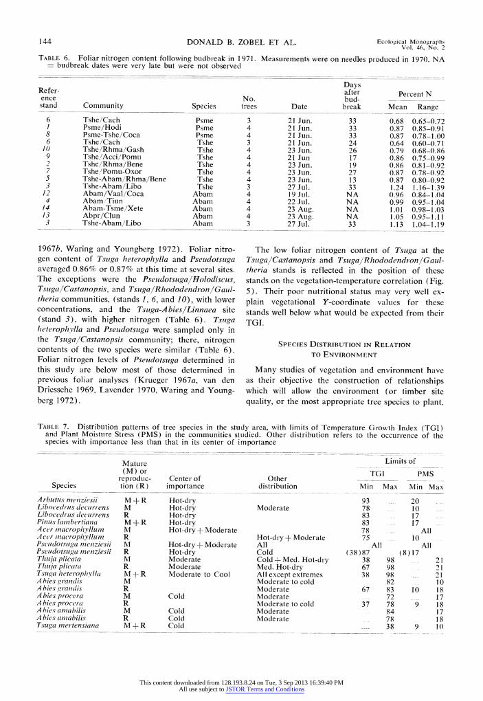
Site differences in nutrient availability should be clearest following bud burst, when 1-yr-old leaves lose some of their nutrients to developing shoots (Krueger
This content downloaded from 128.193.8.24 on Tue, 3 Sep 2013 16:39:40 PMAll use subject to JSTOR Terms and Conditions
144 DONALD B. ZOBEL ET AL. Ecological Monographs Vol. 46, No. 2
TABLE 6. Foliar nitrogen content following budbreak in 1971. Measurements were on needles produced in 1970. NA budbreak dates were very late but were not observed
Days Refer- after Percent N ence No. bud- stand Community Species trees Date break Mean Range
6 Tshe/Cach Psme 3 21 Jun. 33 0.68 0.65-0.72 I Psme/Hodi Psme 4 21 Jun. 33 0.87 0.85-0.91 8 Psme-Tshe/Coca Psme 4 21 Jun. 33 0.87 0.78-1.00 6 Tshe/Cach Tshe 3 21 Jun. 24 0.64 0.60-0.71
10 Tshe/Rhma/Gash Tshe 4 23 Jun. 26 0.79 0.68-0.86 9 Tshe,/Acci/Pomu Tshe 4 21 Jun. 17 0.86 0.75-0.99 2 Tshe/Rhma/Bene Tshe 4 23 Jun. 19 0.86 0.81-0.92 7 Tshe/Pomu-Oxor Tshe 4 23 Jun. 27 0.87 0.78-0.92 5 Tshe-Abam/Rhma/Bene Tshe 4 23 Jun. 13 0.87 0.80-0.92 3 Tshe-Abam/Libo Tshe 3 27 Jul. 33 1.24 1.16-1.39
12 Abam/Vaal/Coca Abam 4 19 Jul. NA 0.96 0.84-1.04 4 Abam//Tiun Abam 4 22 Jul. NA 0.99 0.95-1.04
14 Abam-Tsme/Xete Abam 4 23 Aug. NA 1.01 0.98-1.03 13 Abpr/Clun Abam 4 23 Aug. NA 1.05 0.95-1.11 3 Tshe-Abam/Libo Abam 3 27 Jul. 33 1.13 1.04-1.19
1967b, Waring and Youngberg 1972). Foliar nitro- gen content of Tsuga heterophylla and Pseudotsuga averaged 0.86% or 0.87% at this time at several sites. The exceptions were the PseudotsugalHolodiscus, Tsuga/Castanopsis, and TsugalRhododendron/Gaul- theria communities, (stands 1, 6, and 10), with lower concentrations, and the Tsuga-Abies/Linnaea site (stand 3), with higher nitrogen (Table 6). Tsuga heterophylla and Pseudotsuga were sampled only in the Tsuga/Castanopsis community; there, nitrogen contents of the two species were similar (Table 6). Foliar nitrogen levels of Pseudotsuga determined in this study are below most of those determined in previous foliar analyses (Krueger 1967a, van den Driessche 1969, Lavender 1970, Waring and Young- berg 1972).
The low foliar nitrogen content of Tsuga at the TsugalCastanopsis and TsugalRhododendronlGaul- theria stands is reflected in the position of these stands on the vegetation-temperature correlation (Fig. 5). Their poor nutritional status may very well ex- plain vegetational Y-coordinate values for these stands well below what would be expected from their TG1.
SPECIES DISTRIBUTION IN RELATION TO ENVIRONMENT
Many studies of vegetation and environment have as their objective the construction of relationships which will allow the environment (or timber site quality, or the most appropriate tree species to plant,
TABLE 7. Distribution patterns of tree species in the study area, with limits of Temperature Growth Index (TGI) and Plant Moisture Stress (PMS) in the communities studied. Other distribution refers to the occurrence of the species with importance less than that in its center of importance
Mature Limits of (M) or TG1 PMS
reproduc- Center of Other __ T P Species tion (R) importance distribution Min Max Min Max
A rbutus mernziesii M + R Hot-dry 93 20 Libocedlrus decurrens M Hot-dry Moderate 78 10 Libocedlrus tlecurrens R Hot-dry 83 17 Pinus lambertiana M + R Hot-dry 83 17 A cer macrophyllumn M Hot-dry + Moderate 78 All A cer nacrophylluni R Hot-dry + Moderate 75 10 Pseudlotsuga menziwsii M Hot-dry + Moderate All All All Pseudotsuga menziesii R Hot-dry Cold (38 ) 87 (8)17 Thuja plicata M Moderate Cold+ Med. Hot-dry 38 98 21 Thuja plicata R Moderate Med. Hot-dry 67 98 21 Tsuga heterophyllil M+R Moderate to Cool All except extremes 38 98 21 A bies graml/is M Moderate to cold 82 10 Abies aranldis R Moderate 67 83 10 18 Abies procera M Cold Moderate 72 17 A bies procera R Moderate to cold 37 78 9 18 Abies arnabilis M Cold Moderate 84 17 A bies aniabilis R Cold Moderate 78 18 Tsuga mertensiana M+R Cold 38 9 10
This content downloaded from 128.193.8.24 on Tue, 3 Sep 2013 16:39:40 PMAll use subject to JSTOR Terms and Conditions
Spring 1976 FOREST COMMUNITIES AND ENVIRONMENT 145
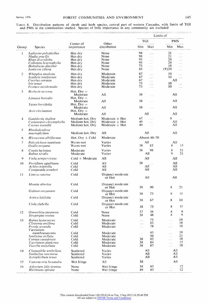
TABLE 8. Distribution patterns of shrub and herb species, central part of western Cascades, with limits of TGI and PMS in the communities studied. Species of little importance in any community are excluded
Limits of
TGI PMS Center of Other
Group Species importance distribution Min Max Min Max
1 Lath yrus polyvphyllus Hot-dry None 98 21 AMadia gracilis Hot-dry None 98 21 Rims dli'ersiloba Hot-dry None 93 20 Collonzia heterophylla Hot-dry None 93 20 Holodiscus discolor Hot-dry None 73 18 Lonicera ciliosa Hot-dry None 83 (9)20
2 Whipplia modesta Hot-dry Moderate 67 10 Synthris reniforniis Hot-dry Moderate 67 10 Corvlis cornuta Hot-dry Moderate 67 All Iris tenax Hot-dry Moderate 73 10 Festuca occidlentalis Hot-dry Moderate 73 10
3 Berberis nervosa Hot, Dry + Moderate All 38 All
Linnaea borealis Hot, Dry + Moderate All 38 All
Taxus brevifolia Hot, Dry + Moderate All 38 All
A cer circinatumi Hot, Dry + Moderate All All All
4 Gaultheria shallon Medium hot, Dry Moderate + Hot 67 9 Castanopsis chrysophylla Medium hot, Dry Moderate + Hot 49 All Cornus nuttaiji Medium hot, Dry Moderate + Hot 49 All
5 Rhododendron macrophylum Medium hot, Dry All All All
6 Hieraceuin (ilbiflorum IHot, Dry + Cold Moderate Absent 40-70
7 Polvstichum inunitum Warn-wet Varies All All Oxalis oregana Warm-wet Varies 38 83 8 15
8 Coptis laciniata Moderate Varies 38 98 8 21 Rubus nix'alis Moderate Varies All 9 2 1
9 Viola semperv'irens Cold + Moderate All All All
10 Pteritliun aquilinuin Cold All 38 All A chl s triphylla Cold All All All Camnpanula scouleri Cold All All All
1I Listera caurina Cold Disjunct moderate or Hot All All
Mon tial siberica Cold Disjunct moderate or Hot 38 90 8 21
Galiul oreganum Cold Disjunct moderate orHot 38 73 8 15
A rnica latifolia Cold Disjunct moderate or Hot 38 67 8 10
Viola glabella Cold Disjunct moderate or Hot 38 73 8 15
12 Osmiiorhiza purpurea Cold None 37 38 8 9 Streptopus roseus Cold None 38 48 8 9
13 Rubits lasiococcus Cold Moderate 73 18 Clintonia uniiflora Cold Moderate 83 1 8 Pv'rola secunda Cold Moderate 78 18 Vacciniuin
mnembranaceum Cold Moderate 93 19 Smilicina stellata Cold Moderate 98 21 Cornus canadensis Cold Moderate 38 82 18 Vaccinium alaskense Cold Moderate 38 84 - 15 Tiarella unifoliata Cold Moderate 38 87 18
1 4 Chimnphila unibellata Scattered Varies All All Smilacina racemiosa Scattered Varies All All Xeroph illum tenax Scattered Varies All All
1 5 Vancouveria hexandlra Wet fringe All 38 All
16 Athyr~iuii Jilix-fem7ina None Wet fringe 38 83 12 Blevchnunis~ spicantt None Wet fringe 49 83 -- 12
This content downloaded from 128.193.8.24 on Tue, 3 Sep 2013 16:39:40 PMAll use subject to JSTOR Terms and Conditions

146 DONALD B. ZOBEL ET AL. Eco Vogical Monographs
TABLE 8. Continued
Limits of
TGI PMS Center of Other
Group Species importance distribution Min Max Min Max
17 Fragaria vesca var. bracteata None Dry fringe All 10
18 Pyirola asarifolia None 2 of three extremes absent 38 98 21
Pxvrola picta None 2 of three extremes absent 38 93 19
Rosa gymnocarpa None 2 of three extremes absent 38 All
Asarumn caulatum None 2 of three extremes absent 38 87 18
Corallorhiza iniertenlsiana None 2 of three extremes absent 38 82 18
Pachistuia myrsinites None 2 of three extremes absent 38 All
Disporullm hookeri None 2 of three extremes absent 38 98 21l
19 Galilum triflorum None All except coldest 38 All Rublus ursinlus None All except coldest 38 All A/deflocalilon bicolor None All except coldest 38 All Vaccinjitin parvifoliumn None All except coldest 38 All Trientalis latifolia None All except coldest 38 All Symplhoricar-pos inollis None All except coldest 38 All
20 Anemnone deltoidea None All All All Chiniaphila mnenziesii None All All All Tr illium ovatum None All 98 21 Goodvera oblongifolia None All All All
or the best silvicultural technique to use) to be pre- dicted from the flora of the site. In many cases the environmental indexes derived from indicator plants are effective predictors of the measured environmen- tal index (Waring and Major 1964, Griffin 1967, Waring et al. 1972, Minore 1972). However, it is stressed that their use should be confined to the region studied (Griffin 1967, Minore 1972, MacLean and Bolsinger 1973). Within our study area most species grow in a variety of habitats, although some prefer- ential species are recognized (Dyrness et al. 1974). When species importance values are plotted on a TGI- PMS diagram, a number of distributional types emerge (Tables 7 and 8). Species with very low cover or low constancy in all communities were not con- sidered in compiling these data.
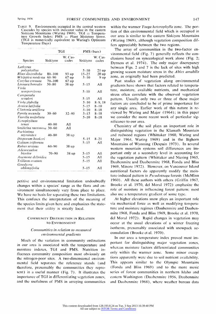
The ranges of TGI and PMS within which a species occurs in our area were compared with the habitat ranges of the species studied elsewhere in the North- west. Most species which Waring (1969) considered sufficiently restricted in distribution to have indicator value were less restricted in our area (Table 9). Most species used as moisture indicators occupied drier environments in our area than they did in the eastern Siskiyous. Several plants used as temperature indi- cators in the Siskiyous extended to both warmer and cooler environments in our study area and almost all occupied warmer habitats. General comparisons pos- sible with other gradient analyses in southern Oregon
(Whittaker 1960, Minore 1972) show the same type of difference, i.e., many species occupying en- vironments relatively drier or warmer in our study area than they do further south. Such differences are not surprising. Higher rainfall and humidity, a shorter dry season, or different competitive pressures in our area may allow the expansion of species into the warmer, drier habitats, as defined by our indexes.
Comparisons with species distribution patterns from the redwood region of California (Waring and Major 1964) reveal no general pattern of differences. Many species have an apparently broader range in our area (Gaultheria shallon, Achlys triphylla, and Acer macrophyllum, for example). Some species (Oxalis oregana and Polystichunm mnunituin) are more restricted to the wetter habitats here than they are in the redwood region. Rhus diversiloba, on the other hand, is more restricted to dry habitats in our study area. Libocedrus decurrens is limited to the warmest (and driest) habitats here, but to the coolest (and driest) in northwestern California.
Interpretation of the significance of these TGI and PMS limits (Tables 7, 8, and 9) is somewhat difficult, as the relative effects of biotic and abiotic factors on range limitation are unknown. Within one small area in the southern Appalachians, some tree species were apparently limited by environment, one by competition, and others by a combination of the two (Mowbray and Oosting 1968). The mix of com-
This content downloaded from 128.193.8.24 on Tue, 3 Sep 2013 16:39:40 PMAll use subject to JSTOR Terms and Conditions
Spring 1976 FOREST COMMUNITIES AND ENVIRONMENT 147
TABLE 9. Environments occupied in the central western Cascades by species with indicator value in the eastern Siskiyou Mountains (Waring 1969). TGi - Tempera- ture Growth Index; PMS - Plant Moisture Stress. (TGI is numerically equivalent to Waring's Optimum Temperature Days)
TGI PMS (bars)
W. Cas- W. Cas- Species Siskiyou cades Siskiyou cades
Lathivrus polyphylflas 5-10 21 up
Rhus div'ersiloba 80-100 93 uip 15-25 20 up Whipplea inodesta 60-90 67 up 5-10 9 up Corvlus cornuta 70-100 67 up Limiaea boreali~s 50-80 38 up 5-15 All Viola
sem pervirens 5-10 All Camn panula
scouleri 5-15 All Viola glabella 5-10 8-9, 18 A rnica latifolia 5-15 8-10 Clintonia uniflora 5-10 8-18 Pyrola secunda 30-60 32-80 5-15 8-18 Tiarella unifoliata 5-10 8-18 Xerophyllumn
tenax 40-80 All Smnilicina racenlosa 30-60 All Pachistimna
myvrsinites 40-80 38 up IDisporalm hookeri 5-15 8-21 Galiulm triflorum 5-15 All Rublbs arsinus 60-90 38 up A denlocaulonl
bicolor 70-90 38 up 5-15 All A ienione deltoidea 5-15 All Trilliuam ov'atam 5-15 All Goodvera
oblongifolia 5-15 All
petitive and environmental limitation undoubtedly changes within a species' range as the flora and en- vironment simultaneously vary from place to place. We have no basis for separating these two limitations. This confuses the interpretation of the meaning of the species limits given here and emphasizes the state- ment that their utility is strictly local.
COMMUNITY DISTRIBUTION IN RELATION
TO ENVIRONMENT
Communities in relation to mneasured environmental gradients
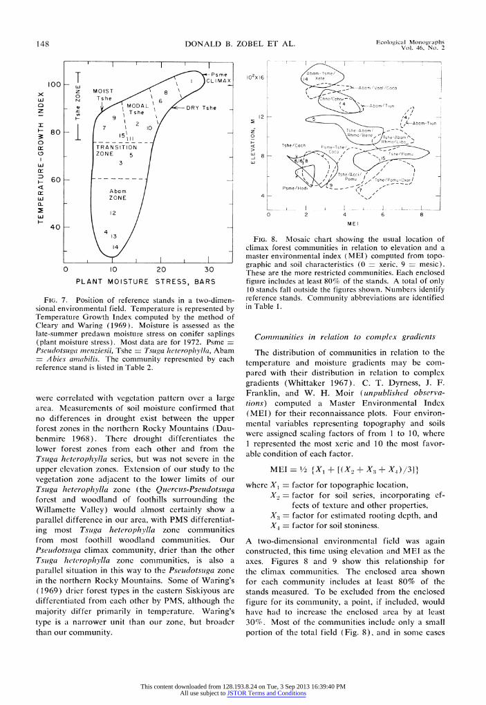
Much of the variation in community ordinations in our area is associated with the temperature and moisture indexes, TG1 and PMS. Nutrition in- fluences community composition most obviously on the nitrogen-poor sites. A two-dimensional environ- mental field separates the reference stands (and therefore, presumably the communities they repre- sent) in a useful manner (Fig. 7). It illustrates the importance of TGI in differentiating vegetation zones, and the usefulness of PMS in arraying communities
within the warmer Tsuga heterophylla zone. The por- tion of this environmental field which is occupied in our area is similar to the eastern Siskiyou Mountains (Waring 1969), although vegetation composition dif- fers appreciably between the two regions.
The array of communities in the two-factor en- vironmental field (Fig. 7) generally reflects the con- clusions based on synecological work alone (Fig. 2; Dyrness et al. 1974). The only major discrepancy between Figs. 2 and 7 is the lack of sites with high growing season moisture stress in the Abies ainabilis zone, as originally had been predicted.
Past studies of vegetation along environmental gradients have shown that factors related to tempera- ture, moisture, available nutrients, and mechanical stress often correlate with the observed vegetation pattern. Usually only two or three of these major factors are concluded to be of prime importance for any single area. Earlier work of this nature is re- viewed by Waring and Major (1964); in this paper we consider the more recent work of particular sig- nificance to our area.
Chemistry of the soil plays an important role in distinguishing vegetation in the Klamath Mountain and redwood regions (Whittaker 1960, Waring and Major 1964, Waring 1969) and in the Bighorn Mountains of Wyoming (Despain 1973). In several western mountain systems soil differences are im- portant only at a secondary level in accounting for the vegetation pattern (Whittaker and Niering 1965, Daubenmire and Dauibenmire 1968, Fonda and Bliss 1969, Minore 1972). However, on Vancouver Island nutritional factors do apparently modify the mois- ture-induced pattern in Pseitdotsuga forests (McMinn 1960). All these authors with others (Griffin 1967, Brooke et al. 1970, del Moral 1972) emphasize the role of moisture in influencing forest pattern; most also use a temperature gradient of some type.
At higher elevations snow plays an important role via mechanical force as well as modifying tempera- ture and moisture regimes (Daubenmire and Dauben- mire 1968, Fonda and Bliss 1969, Brooke et al. 1970, del Moral 1972). Rapid changes in vegetation may occur at the usual elevations of a winter freezing isotherm, presumably associated with snowpack ac- cumulation (Brooke et al. 1970).
In our area a temperature index proved most im- portant for distinguishing major vegetation zones, whereas moisture factors differentiated communities only within the warmer zone. Some minor excep- tions apparently were due to soil nutrient availability. This appears similar to the Olympic Mountains (Fonda and Bliss 1969) and to the more mesic series of forest communities in northern Idaho and eastern Washington (Datubenniire 1956, Daubenmire and DauLbenmire 1968), where weather bureau data
This content downloaded from 128.193.8.24 on Tue, 3 Sep 2013 16:39:40 PMAll use subject to JSTOR Terms and Conditions
148 DONALD B. ZOBEL ET AL. Ecological Monographs
. I I - I I
Psme
Ioo T ,.C L I M A X 10 MOIST 8 I CIA
? 80she<s h
UJ | TRASITION /
0 4) ~~~MODAL DRY Tshe _ ZONE I she
_r 7 1 2 0 F 80 - 1 I - 5 III 0 a: TRANSITION O ZONE 5
LJ- a: D H- 60 -
<: Abam Lii ZONE
2 ~~~~~~12 LU
40 4
'3
0 10 20 30
PLANT MOISTURE STRESS, BARS
FIG. 7. Position of reference stands in a two-dimen- sional environmental field. Temperature is represented by Temperature Growth Index computed by the method of Cleary and Waring (1969). Moisture is assessed as the late-summer predawn moisture stress on conifer saplings (plant moisture stress). Most data are for 1972. Psme = Pseudotsuga menziesii, Tshe = Tsuga heterophylla, Abam
Abies anmabilis. The community represented by each reference stand is listed in Table 2.
were correlated with vegetation pattern over a large area. Measurements of soil moisture confirmed that no differences in drought exist between the upper forest zones in the northern Rocky Mountains (Dau- benmire 1968). There drought differentiates the lower forest zones from each other and from the Tsuga heterophylla series, but was not severe in the upper elevation zones. Extension of our study to the vegetation zone adjacent to the lower limits of our Tsuga heterophylla zone (the Quercus-Pseudotsuga forest and woodland of foothills surrounding the Willamette Valley) would almost certainly show a parallel difference in our area, with PMS differentiat- ing most Tsuga heterophylla zone communities from most foothill woodland communities. Our Pseudotsiiga climax community, drier than the other Tsuga heterophylla zone communities, is also a parallel situation in this way to the Pseudotsuga zone in the northern Rocky Mountains. Some of Waring's (1969) drier forest types in the eastern Siskiyous are differentiated from each other by PMS, although the majority differ primarily in temperature. Waring's type is a narrower unit than our zone, but broader than our community.
102X 16 ab 4 Xete -)
/_A-Abr n/Vc Ia/Coca
hn pho,--
-,bcm Tw iun
i2 '4, So <-Abam/T~~~un .AbmTu
1 2 C =4 I - A b a m
-hT i un
I kshe- 1-cI 0 \Rhmc, Bene- Tshe-AbomA
1, \ (y hma/Libo _ < Tshe/Cach P me-Tshe - ( ha L
11 8 - X
2, he iom
> Ps/ Pomu e / Tshe Pomu- ar /
PsmeH'she/Po-
4 _/o
_ . I 1 1 . . 0 2 4 6 8
Ljj~~~~~~~
FIG. 8. Mosaic chart showing the usual location of climax forest communities in relation to elevation and a master environmental index ( MEl ) computed from topo- graphic and soil characteristics (0 xeric, 9 mesic). These are the more restricted communities. Each enclosed figure includes at least 80% of the stands. A total of only 10 stands fall outside the figures shown. Numbers identify reference stands. Community abbreviations are identified in Table 1.
Communities in relation to complex gradients
The distribution of communities in relation to the temperature and moisture gradients may be com- pared with their distribution in relation to complex gradients (Whittaker 1967). C. T. Dyrness, J. F. Franklin, and W. H. Moir (unpublished observa- tions) computed a Master Environmental Index (MET) for their reconnaissance plots. Four environ- mental variables representing topography and soils were assigned scaling factors of from 1 to 10, where 1 represented the most xeric and 10 the most favor- able condition of each factor.
MEI = 1/2 tX1 + [(X? + X? + X4)3]}
where X1 = factor for topographic location, X., = factor for soil series, incorporating ef-
fects of texture and other properties, X- = factor for estimated rooting depth, and X = factor for soil stoniness.
A two-dimensional environmental field was again constructed, this time using elevation and MET as the axes. Figures 8 and 9 show this relationship for the climax communities. The enclosed area shown for each community includes at least 80% of the stands measured. To be excluded from the enclosed figure for its community, a point, if included, would have had to increase the enclosed area by at least 30%. Most of the communities include only a small portion of the total field (Fig. 8), and in some cases
This content downloaded from 128.193.8.24 on Tue, 3 Sep 2013 16:39:40 PMAll use subject to JSTOR Terms and Conditions

Spring 1976 FOREST COMMUNITIES AND ENVIRONMENT 149
102X16 [ I - I I
Abam/Actr a C
1 2 L ->--- A~~~2 Aba m /VaalI/Coc~a / 12
I? 2 Abam /Rhma-Vaal /Coca / Abam/Rhma- l oca i
O 2
0 9she-Abam oLbo
< 2- 17~~0
> 8 TshetRhma-1 com maiBene/ veyi are
Howver there ar eea omuiiswt
_j ~~~~Gash1
4
0 2 4 6 8
M El
FIG. 9. Same as Fig. 8, showing locations of five widely distributed climax communities.
the overlap between communities is not very large. However, there are several communities with a
broad or a bimodal MEI distribution (Fig. 9) which greatly overlap some of the more restricted com- munities. The bimodal nature is a consequence of variation in topographic location, not the soil factors included in MEL.
Comparison with the PMS-TGI ordination shows several differences between the two methods of de- fining the environmental field (Figs. 8 and 9 vs. Fig.
7). The complex-gradient diagram suggests that the mid- to high-elevation communities are mostly xeric, whereas the PMS at all those measured is quite low. At lower elevations the MEI axis shows differences between communities which are relatively smaller than those shown by PMS. The temperature dif- ferences between zones and the temperature patterns within zones are not as apparent using the elevational axis. Of course, some overlap in communities could be expected if several stands per community were measured for PMS and TGI, but this probably would not correct the distortions mentioned above. The MEI axis, constructed to represent a mesic to xeric
scale, has different meanings at different elevations in terms of actual moisture stress.
The dispersion of the five climax communities which show a bimodal distribution on Figs. 8 and 9 is more restricted if one uses a Soil Profile Index
(SPI - [X) + X3 + X41/3) as the X-axis, rather than MEL. All the seral communities are better
separated by SPI than by MEI (Fig. 10). Their pat-
tern of occurrence is probably greatly influenced by
historical factors. The single community at low ele-
vations occupies a very wide range of soil variation.
Advantages of measured environmental gradients
Using measured environmental gradients has several definite advantages, although many workers
102 X 16 T_ I [ T
abpr r
Abpr/Clun 13
I? 2
Z Psme/Acci/Whmo
o Psme/Acci/') Bene ,
U8
Psme/Acci /Gash
4
0 2 4 6 8
SPI
FIG. 10. Mosaic chart showing locations of five seral forest communities in relation to elevation and a soil profile index (SPI) (O = xeric, 9 = mesic).
choose to identify only complex gradients rather than measuring one or a few factors to represent the en- vironmental changes along these gradients. One would expect an elevational complex-gradient in our area to consist substantially of temperature-related factors, with modifications in intensity related to the depth and persistence of the snowpack. The com- plex gradient referred to in topographic terms is pri- marily a moisture gradient (Whittaker 1967). In many cases no single factor can be isolated which varies over the entire gradient of vegetation (John- son and Risser 1972), making measurement of two or more factors imperative. That one or two mea- sured factors do correlate well with the vegetation gradient does not necessarily imply that they are the sole causal agent(s) of the pattern, of course. For example, Mowbray and Oosting (1968) found the
clay/sand ratio in the soil to be the factor best cor- related with tree importance and growth. Their dis- cussion emphasizes that besides direct influences on plants via soil aeration and moisture retention, this ratio integrated many microclimatic factors operating over a long time.
Despite the uncertainty as to the degree of causal influence that a measured environmental factor has, we believe that gradient quantification is a worthwhile endeavor. A working knowledge of the nature of effective environmental gradients is necessary to gain understanding of the adaptive strategies of the popu- lations involved and to generate testable hypotheses about the specific competitive and selective forces acting on these populations. For example, a moisture gradient may involve either (or both) atmospheric and soil moisture. Adaptive responses to a moisture gradient vary depending on the exact nature of the gradient. Grand fir saplings on the more arid east slope of the Oregon Cascades are indeed subject to
This content downloaded from 128.193.8.24 on Tue, 3 Sep 2013 16:39:40 PMAll use subject to JSTOR Terms and Conditions
150 DONALD B. ZOBEL ET AL. Ecological Mo nographs Vol. 46, No. 2
greater evaporative stress than west slope populations, but maximum measured plant moisture stresses are below those of west-slope populations, the reverse of the situation expected. These populations exhibit stomatal reaction patterns which are related to the differences in the type of moisture stress to which they are subjected (Zobel 1974. 1975).
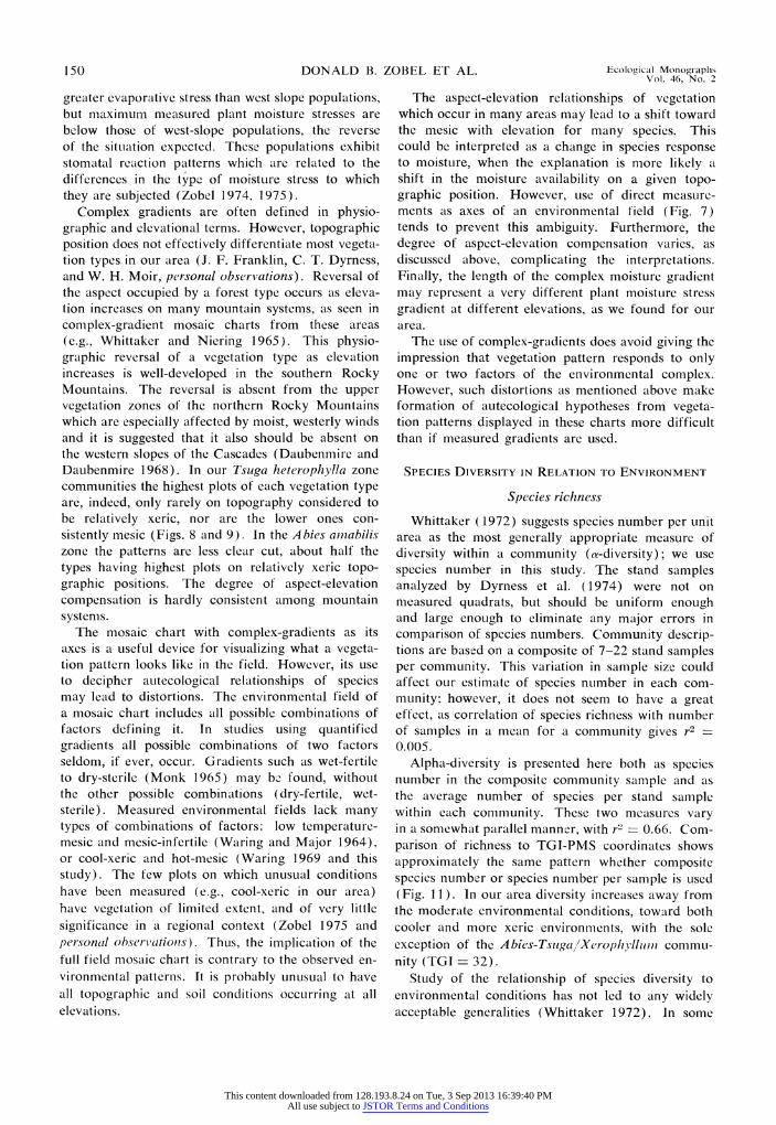
Complex gradients are often defined in physio- graphic and elevational terms. However, topographic position does not effectively differentiate most vegeta- tion types in our area (J. F. Franklin, C. T. Dyrness, and W. H. Moir, personal observations). Reversal of the aspect occupied by a forest type occurs as eleva- tion increases on many mountain systems, as seen in complex-gradient mosaic charts from these areas (e.g., Whittaker and Niering 1965). This physio- graphic reversal of a vegetation type as elevation increases is well-developed in the southern Rocky Mountains. The reversal is absent from the upper vegetation zones of the northern Rocky Mountains which are especially affected by moist, westerly winds and it is suggested that it also should be absent on the western slopes of the Cascades (Daubenmire and Daubenmire 1968). In our Tsuga heterophylla zone communities the highest plots of each vegetation type are, indeed, only rarely on topography considered to be relatively xeric, nor are the lower ones con- sistently mesic (Figs. 8 and 9). In the Abies ainabilis zone the patterns are less clear cut, about half the types having highest plots on relatively xeric topo- graphic positions. The degree of aspect-elevation compensation is hardly consistent among mountain systems.
The mosaic chart with complex-gradients as its axes is a useful device for visualizing what a vegeta- tion pattern looks like in the field. However, its use to decipher autecological relationships of species may lead to distortions. The environmental field of a mosaic chart includes all possible combinations of factors defining it. In studies using quantified gradients all possible combinations of two factors seldom, if ever, occur. Gradients such as wet-fertile to dry-sterile (Monk 1965) may bKi found, without the other possible combinations (dry-fertile, wet- sterile). Measured environmental fields lack many types of combinations of factors: low temperature- mesic and mesic-infertile (Waring and Major 1964), or cool-xeric and hot-mesic (Waring 1969 and this study). The few plots on which unusual conditions have been measured (e.g., cool-xeric in our area) have vegetation of limited extent, and of very little significance in a regional context (Zobel 1975 and personal observations). Thus, the implication of the full field mosaic chart is contrary to the observed en- vironmental patterns. It is probably unusual to have all topographic and soil conditions occurring at all elevations.
The aspect-elevation relationships of vegetation which occur in many areas may lead to a shift toward the mesic with elevation for many species. This could be interpreted as a change in species response to moisture, when the explanation is more likely a shift in the moisture availability on a given topo- graphic position. However, use of direct measure- ments as axes of an environmental field (Fig. 7) tends to prevent this ambiguity. Furthermore, the degree of aspect-elevation compensation varies, as discussed above, complicating the interpretations. Finally, the length of the complex moisture gradient may represent a very different plant moisture stress gradient at different elevations, as we found for our area.
The use of complex-gradients does avoid giving the impression that vegetation pattern responds to only one or two factors of the environmental complex. However, such distortions as mentioned above make formation of autecological hypotheses from vegeta- tion patterns displayed in these charts more difficult than if measured gradients are used.
SPECIES DIVERSITY IN RELATION TO ENVIRONMENT
Species richness
Whittaker ('1972) suggests species number per unit area as the most generally appropriate measure of diversity within a community (a-diversity); we use species number in this study. The stand samples analyzed by Dyrness et al. (1974) were not on measured quadrats, but should be uniform enough and large enough to eliminate any major errors in comparison of species numbers. Community descrip- tions are based on a composite of 7-22 stand samples per community. This variation in sample size could affect our estimate of species number in each com- munity; however, it does not seem to have a great effect, as correlation of species richness with number of samples in a mean for a community gives r2 0.005.
Alpha-diversity is presented here both as species number in the composite community sample and as the average number of species per stand sample within each community. These two measures vary in a somewhat parallel manner, with r2 = 0.66. Com- parison of richness to TGI-PMS coordinates shows approximately the same pattern whether composite species number or species number per sample is used (Fig. 11). In our area diversity increases away from the moderate environmental conditions, toward both cooler and more xeric environments, with the sole exception of the Abies-TsugalXe rophlivlliin commuL-
nity (TGI - 32). Study of the relationship of species diversity to
environmental conditions has not led to any widely acceptable generalities (Whittaker 1972). In some
This content downloaded from 128.193.8.24 on Tue, 3 Sep 2013 16:39:40 PMAll use subject to JSTOR Terms and Conditions

Spring 1976 FOREST COMMUNITIES AND ENVIRONMENT 151
100 31
/ 32 /
0 6
a 543 0 Tshe ZON E
59 2 2 52/ i_80 _ 22 56 66
1
0 a: 52 0 74 21 TRANSITION ZONE
L~~~~~ ~27
60- LAU
E 26 Abam ZONE
H 40 _ 74 70 30 35
39
0 10 20 30
PLANT MOISTURE STRESS, BARS
FIG. 11. Vascular species diversity (number of spe- cies) of forest communities in relation to temperature and moisture conditions at the reference stand representing it. The top figure is the species number in the composite sample; the bottom is the average species number per stand sampled. The reference stand at each position is identified in Fig. 7.
cases diversity is highest in more mesic communities; in others it is not. Terborgh (1973) states that the general case in temperate North American vegeta- tion is to have greatest species number in the middle part of a moisture gradient, rather than in wetter or drier areas. This is contradicted by our study as well as several others (cited in Whittaker 1972, del Moral 1972). One must consider the relative xeric-mesic- hydric range which occurred in each study. In our area the wettest sites did not appear too wet for optimum growth of the dominants. This is probably also true in Whittaker's studies cited by Terborgh (1973). However, in other studies he cites very wet areas were included. A comparison of diversities at the midranges of moisture gradients which have greatly different end-points of hydrism and xerism (Terborgh 1973) should not, it seems, allow strong inference from the results.
Often, diversity in one stratum of vegetation can- not be predicted from the diversities of the other strata (Whittaker 1972). This is also true for this study. That diversities of different strata are un- related is indicated by the r2 between species richness of layers: tree-shrub = 0.01, shrub-herb = 0.02, and tree-herb = 0.06.
The dominance of one stratum (as opposed to its
diversity) may affect the diversity of another (Whit- taker 1972). The greater herb diversity on dry sites in our area contrasts to findings for some temperate forests (Daubenmire and Daubenmire 1968), but is similar to others (Rochow 1972). This pattern may result from a less dense canopy cover over these dry sites, leading to greater light intensities. The re- duced tree density should also cause greater avail- ability of nutrients and water, less chance of al- lelopathic influence, and a greater variety of available microhabitats (Daubenmire and Daubenmire 1968, del Moral 1972, Rochow 1972, Whittaker 1972). In our study the number of herbaceous species was inversely related to the percent cover of evergreen trees and shrubs in the community (r2 = 0.38, n - 22, excluding the A bies-TsugalXerophyllurn commu- nity). Using seral communities alone this r2 was 0.74 (n - 5). The model for control of forest species diversity (del Moral 1972) suggests that con- ditions on our Pseudotsuga climax and Abies arnabilis zone sites are rigorous enough to cause a more open canopy, but are not rigorous enough to greatly deplete the flora. The net effect is increased diversity. The Abies-Tsuga/Xerophyllum community, on the other hand, apparently has an environment rigorous enough to delete many of the less hardy species, thus decreas- ing diversity.
On a given site in many temperate forests, species richness may increase for some time, and then de- crease with canopy closure and establishment of strong dominance (Whittaker 1972). In our area the seral communities average more species than the old-growth communities (68 vs. 60 total; 29 vs. 25 per stand).
The degree to which species composition changes along environmental gradients within an area is termed /3-diversity. A simple and generally appropri- ate measure of /3-diversity is (BD - 1.0), where BD -
ScIS, Sc being the number of species in the composite sample and S the average number of species in the communities (Whittaker 1972). The total vascular B-diversity of our study area is 1.473. a9-diversity is somewhat lower for trees and shrubs (1.26 and 1.25) and higher for herbs (1.63).
Gamma diversity is the species richness in a par- ticular range of habitats. The forests studied by Dyrness et al. (1974) include 153 vascular species. However, the total flora is much larger and is prob- ably estimated best from Franklin and Dyrness (1971) who list 480 vascular plants in the H. J. An- drews Forest. This latter number includes a few introduced tree species and many species character- istic of meadows and disturbed areas (e.g., clearcuts).
Species dominance
Communities vary in the degree to which some measure of importance is shared among the species
This content downloaded from 128.193.8.24 on Tue, 3 Sep 2013 16:39:40 PMAll use subject to JSTOR Terms and Conditions

152 DONALD B. ZOBEL ET AL. Ecological Monographs Vol. 46, No. 2
toop 10
Z 0.14 0.08 Tshe ZONE /0 14 0 140.17/
I 8 0 0.1 0. Z 0 .7 >_60 0 1 ~~~016--15
0
0 _0.15 TRANSITION ZONE
2 ~~~~~0.07 iW 0.16 Abam ZONE H 40
~~0.06o006 0.090 .12
0.52 0.25
0 10 20 30
PLANT MOISTURE STRESS, BARS
FIG. 12. Dominance (Simpson's index) in relation to temperature and moisture conditions of the reference stands representing each community. The top figure is calculated for all vascular species; the bottom for shrubs and herbs only. Percent cover is the measure of im- portance.
present, called equitability, or conversely, the con- centration of dominance. We chose a simple measure of the concentration of dominance, Simpson's index (C).
C -= p,Pi where s is number of species in the collec-
tion and pi is the proportion of the importance value belonging to the ith species. Whittaker (1972) sug- gests that this index is appropriate for communities exhibiting strong dominance, as ours do. We used average percent cover in the composite community sample as our measure of importance.
Dominance varies considerably among commu- nities (Fig. 12), generally being more pronounced in lower elevation and seral stands: Abies amnabilis zone C = 0.115, Tsuga heterophylla zone C = 0.140; seral communities C - 0.148, climax communities C = 0.126. However, the Abies-TsugalXerophylluin community, which is excluded from the means, has a very high dominance. When tree species are excluded from the calculations, the same generality holds for zones, but the understory dominance is similar in both seral and climax stands. Vascular dominance, and
especially understory dominance, generally decrease away from the area of moderate environment toward
60 _TvT iT
40
20
10 8
4
0B
2 D
I ~~~~~~~~~~~~~~~~~~~~6
0 8 _ \ 5 12 15 10 9 A 7 C 2 4 8 3 E
06 A \Abom/Rhmo-Vaol/Coca B \Abom/Actr
04 C Abam/Vame/Xete D Chno/Opho
14 E Tshe-Abam/Rhma/Libo 5
0.2 I J 1i L J. I I I I I I I I I I I
SPECIES RANK
FIG. 13. Dominance-diversity curves for climax com- munities in the central western Cascades, constructed for the 20 most important species in the composite sample for each community. Curves are ordered by the percent cover of the 10th species, from lowest to highest (i.e., approximately the steepest to flattest slope in the top half of the line). Numbers refer to reference stands. Tables 1 and 2 identify communities.
the dry and the cold communities (Fig. 12). Thus, species richness and dominance are generally nega- tively related. C values are generally in the range of those found by del Moral ('1972) for the Wenatchee Mountains.
DOMINANCE-DIVERSITY CURVES
Another way to look at dominance-diversity re- lationships is to plot the log of importance of species (cover, in our case) over species rank of importance. Different shapes of the resulting curve should theo- retically arise depending on the type of theory one invokes for determining how niches are occupied (Whittaker 1972). Curves for the 20 most important species of each composite community sample (Dyr- ness et al. 1974) are of a form generated by a geo- metric series (Fig. 1 3), theoretically produced by the hypothesis of niche-preemption. Such a form is often exhibited by vascular plant communities of low diversity (Whittaker 1972). All our curves have a somewhat similar, steep initial slope. However, all except one have at least two parts with the slope de- creasing after 3-10 species. This broken curve ap- pears to represent two groups of plants: the first group is the dominant trees and the most important understory species, the other the rest of the lower strata. These groups have somewhat different domi- nance relationships as indicated by the slope of the lines, with the less important species groups having a smaller degree of dominance.
This content downloaded from 128.193.8.24 on Tue, 3 Sep 2013 16:39:40 PMAll use subject to JSTOR Terms and Conditions
Spring 1976 FOREST COMMUNITIES AND ENVIRONMENT 153
100
X 41
sheZN
z _ ~~~~~86 ( 100 10 TRANSITION ZONE
D~~~ ~~ 60 0 742j
8 0 _ \3 104 9/
0~
_U Aba ZONE ,
H40 89 6
0 10 20 30
PLANT MOISTURE STRESS, BARS
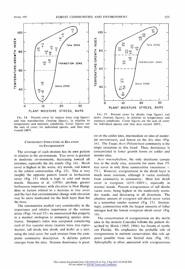
FIG. 14. Percent cover by mature trees (top figure) and tree reproduction (bottom figure ), in relation to temperature and moistuire conditions. Cover figures are the sum of cover for individual species, and thus may exceed 100%.
COMMUNITY STRUCTURE IN RELATION
TO ENVIRONMENT
The coverage of each stratum has its own pattern in relation to the environment. Tree cover is greatest in moderate environments, decreasing toward all extremes, especially the dry stands (Fig. 14). Shrub cover is highest in the warm, dry stands, and lowest in the coldest communities (Fig. 15). This is very roughly the opposite pattern found in herbaceous cover ( Fig. 15 ) which is high in cold and mesic stands. Siccama et al. ( 1970) attribute greater herbaceous importance with elevation in New Hamp- shire to factors related to a decrease in tree cover and the fact that environmental change with elevation may be more moderated for the herb layer than for the trees.
The communities studied vary considerably in the importance and relative importance of the various strata ( Figs. 14 and 1 5 ); we summarized this property in a manner analogous to computing species dom- inance. Simpson's index was computed considering each of five vascular strata (mature trees, tree repro- duction, tall shrub, low shrub, and herb) as a unit, using the total cover for each stratum from the com- posite community description. A definite pattern emerges from the data. Stratum dominance is great-
, I , I l I
100 3
| 8 0 94 K 26816
g / ~~~~~TANSITIONE ZN
F 40 _ i8067 /
0 10 20 30
PLANT MOISTURE STRESS, BARS
FIG. 15. Percent cover by shrubs (top figure) and herbs ( bottom figure ), in relation to temperature and moisture conditions. Cover figures are the sum of cover for individual species and thus may exceed 100%.
est on the colder sites, intermediate on sites of moder- ate environment, and lowest on the dry sites (Fig. 16). The Tsugsa Acer Poly~stichluin community is the single exception to this trend. Thus, dominance is concentrated in fewer growth forms on colder and moister sites.
Acser inacro phylluin, the only deciduous canopy tree in the study area, accounts for more than 3% tree cover in only three communities (maximum -
7%X). However, evergreenness in the shrub layer is much more common, although it varies markedly from community to community. Most low shrub cover is evergreen (63%-100% ), especially in warmer stands. Percent evergreenness of tall shrubs varies more, being highest in the moderately warm- dry stands, and decreasing in all directions. The absolute amount of evergreen tall shrub cover varies in a somewhat similar manner (Fig. 17). Interest- ingly, communities with the largest amounts of foliar nitrogen had the lowest evergreen shrub cover (Fig. 18).
The concentration of evergreenness on dry sterile sites in the western Cascades follows the pattern de- scribed by Monk (1965, 1966) for forests of north- ern Florida. He emphasizes the probable role of evergreenness in nutrient conservation; this role ap- pears possible from our limited data ( Fig. 1 8) . Sclerophylly is often associated with evergreen ness;
This content downloaded from 128.193.8.24 on Tue, 3 Sep 2013 16:39:40 PMAll use subject to JSTOR Terms and Conditions

154 DONALD B. ZOBEL ET AL. Ecological Monographs Vol. 46, No. 2
100
X /0.28/ LAJ
Z / .7/ Tshe ZONE 0~~~~~~~~03
80 0.33 0.38
0.2
0
0.32 TRANSITION ZONE
D60 0O4 cl&
W
a.. 0.40
L4| Abam ZONE H40
0.37 0.38
0.8
0 10 20 30
PLANT MOISTURE STRESS, BARS
FIG. 16. Stratum dominance: Simpson's index com- puted for percent cover of five layers (mature tree, tree reproduction, tall shrub, low shrub, and herb), in relation to temperature and moisture conditions.
its importance in moisture conservation appears to be of secondary importance, or at least to be ineffective on our driest areas. The percentage of evergreenness is low in our two driest communities.
SOME IMPLICATIONS OF PATTERNS OF
STRUCTURE AND DIVERSITY
The different community properties which we have examined exist in a variety of patterns over the en- vironmental field we defined. Species richness in- creases toward our environmental extremes, whereas tree coverage and concentration of dominance de- crease toward these extremes. Stratum dominance, shrub cover, and herbaceous cover vary in a more unidirectional manner across the environmental gradients. Shrub cover is highest on warm, dry sites, and the other two are highest on the cooler, moister sites. The pattern of diversity within a single stratum varies in a manner unrelated to diversity of other strata; however, herbaceous diversity is related to the coverage of evergreen shrubs and trees.
The Abies-TsugalXerophylluin community (refer- ence stand 14), although the coldest we measured, still has environmental indexes not very different from the Abies amabilis zone stands. This is reflected in the pattern of structural characteristics: the trends set by the adjoining stands extend to stand 14 (Figs. 14, 15, and 16). However, this is not true for the
I 80 t 36 I1
100 2
a _6X8
LAJ 5
0 30 0 P 10 TRANSITION ZONE LAJ
I-
CLA
iAJ 6 Abam ZONE ~40 0 0 5
0
0 10 20 30 PLANT MOISTURE STRESS, BARS
FIG. 17. Percent cover by tall (top figure) and low (bottom figure) evergreen shrubs, in relation to tempera- ture and moisture conditions.
general trends for diversity (Figs. 11 and 12), which reverse themselves at stand 14. The sharp discon- tinuities which occur here reinforce the conclusion, based on composition, that this community really represents a different vegetational zone (the Tsuga mertensiana zone of Franklin and Dyrness 1973) and suggest that major changes occur here which are not reflected in our environmental indexes. If such dis-
; 80 I I I
w A-TALL
o 60 O-LOW 0 6
I 40 en
20 A
w ~~0 > 0 0.8 1 1.2
FOLIAR N CONTENT, %
FIG. 18. Percent cover by evergreen shrubs in rela- tion to summer N contents of needles of conifer saplings. Nutrient data are for Tsuga heterophylla or Pseudotsuga menziesii.
This content downloaded from 128.193.8.24 on Tue, 3 Sep 2013 16:39:40 PMAll use subject to JSTOR Terms and Conditions
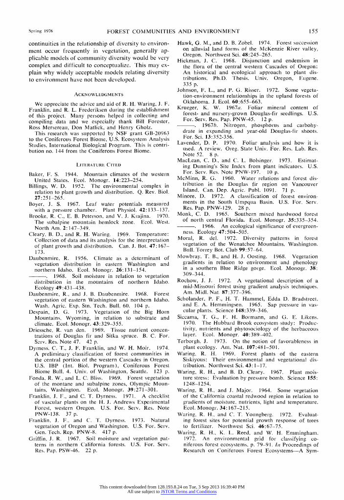
Spring 1976 FOREST COMMUNITIES AND ENVIRONMENT 155
continuities in the relationship of diversity to environ- ment occur frequently in vegetation, generally ap- plicable models of community diversity would be very complex and difficult to conceptualize. This may ex- plain why widely acceptable models relating diversity to environment have not been developed.
ACKNOWLEDGMENTS
We appreciate the advice and aid of R. H. Waring, J. F. Franklin, and R. L. Frederiksen during the establishment of this project. Many persons helped in collecting and compiling data and we especially thank Bill Forester, Ross Mersereau, Don Matlick, and Henry Gholz.
This research was supported by NSF grant GB-20963 to the Coniferous Forest Biome, U.S. Ecosystem Analysis Studies, International Biological Program. This is contri- bution no. 144 from the Coniferous Forest Biome.
LITERATURE CITED
Baker, F. S. 1944. Mountain climates of the western United States. Ecol. Monogr. 14:223-254.
Billings, W. D. 1952. The environmental complex in relation to plant growth and distribution. Q. Rev. Biol. 27: 251-265.
Boyer, J. S. 1967. Leaf water potentials measured with a pressure chamber. Plant Physiol. 42:133-137.
Brooke, R. C., E. B. Peterson. and V. J. Krajina. 1970. The subalpine mountain hemlock zone. Ecol. West. North Am. 2:147-349.
Cleary. B. D., and R. H. Waring. 1969. Temperature: Collection of data and its analysis for the interpretation of plant growth and distribution. Can. J. Bot. 47:167- 173.
Daubenmire, R. 1956. Climate as a determinant of vegetation distribution in eastern Washington and northern Idaho. Ecol. Monogr. 26:131-154.
1968. Soil moisture in relation to vegetation distribution in the mountains of northern Idaho. Ecology 49:43 1-438.
Daubenmire, R., and J. B. Daubenmire. 1968. Forest vegetation of eastern Washington and northern Idaho. Wash. Agric. Exp. Stn. Tech. Bull. 60. 104 p.
Despain, D. G. 1973. Vegetation of the Big Horn Mountains. Wyoming, in relation to substrate and climate. Ecol. Monogr. 43:329-355.
Driessche, R. van den. 1969. Tissue nutrient concen- trations of Douglas fir and Sitka spruce. B. C. For. SIrv. Res. Note 47. 42 p.
Dyrness, C. T., J. F. Franklin, and W. H. Moir. 1974. A preliminary classification of forest communities in the central portion of the western Cascades in Oregon. U.S. IBP (Int. Biol. Program), Coniferous Forest Biome Bull. 4. Univ. of Washington, Seattle. 123 p.
Fonda. R. W., and L. C. Bliss. 1969. Forest vegetation of the montane and subalpine zones, Olympic MouLn- tains, Washington. Ecol. Monogr. 39:271-301.
Franklin, J. F., and C. T. Dyrness. 1971. A checklist of vascular plants on the H. J. Andrews Experimental Forest, western Oregon. U.S. For. Serv. Res. Note PNW-138. 37 p.
Franklin. J. F.. and C. T. Dyrness. 1973. Natural vegetation of Oregon and Washington. U.S. For. Serv. Gen. Tech. Rep. PNW-8. 417 p.
Griffin. J. R. 1967. Soil moisture and vegetation pat- terns in northern California forests. U.S. For. Serv. Res. Pap. PSW-46. 22 p.
Hawk, G. M., and D. B. Zobel. 1974. Forest succession on alluvial land forms of the McKenzie River valley, Oregon. Northwest Sci. 48:245-265.
Hickman, J. C. 1968. Disjunction and endemism in the flora of the central western Cascades of Oregon: An historical and ecological approach to plant dis- tributions. Ph.D. Thesis. Univ. Oregon, Eugene. 335 p.
Johnson, F. L., and P. G. Risser. 1972. Some vegeta- tion-environment relationships in the upland forests of Oklahoma. J. Ecol. 60:655-663.
Krueger, K. W. 1967a. Foliar mineral content of forest- and nursery-grown Douglas-fir seedlings. U.S. For. Serv. Res. Pap. PNW-45. 12 p.
1967b. Nitrogen, phosphorus and carbohy- drate in expanding and year-old Douglas-fir shoots. For. Sci. 13:352-356.
Lavender, D. P. 1970. Foliar analysis and how it is used. A review. Oreg. State Univ. For. Res. Lab. Res. Note 52. 8 p.
MacLean, C. D., and C. L. Bolsinger. 1973. Estimat- ing Dunning's Site Index from plant indicators. U.S. For. Serv. Res. Note PNW-197. 10 p.
McMinn, R. G. 1960. Water relations and forest dis- tribution in the Douglas fir region on Vancouver Island. Can. Dep. Agric. Publ. 1091. 71 p.
Minore, D. 1972. A classification of forest environ- ments in the South Umpqua Basin. U.S. For. Serv. Res. Pap. PNW-129. 28 p.
Monk, C. D. 1965. Southern mixed hardwood forest of north central Florida. Ecol. Monogr. 35:335-354.
1966. An ecological significance of evergreen- ness. Ecology 47:504-505.
Moral, R. del. 1972. Diversity patterns in forest vegetation of the Wenatchee Mountains, Washington. Bull. Torrey Bot. Club 99:57-64.
Mowbray. T. B., and H. J. Oosting. 1968. Vegetation gradients in relation to environment and phenology in a southern Blue Ridge gorge. Ecol. Monogr. 38: 309-344.
Rochow, J. J. 1972. A vegetational description of a mid-Missou ri forest using gradient analysis techniques. Am. Midl. Nat. 87:377-396.
Scholander, P. F., H. T. Hammel, Edda D. Bradstreet. and E. A. Hemmingsen. 1965. Sap pressure in vas- cular plants. Science 148:339-346.
Siccama, T. G., F. H. Bormann, and G. E. Likens. 1970. The Hubbard Brook ecosystem study: Produc- tivity, nutrients and phytosociology of the herbaceous layer. Ecol. Monogr. 40:389-402.
Terborgh. J. 1973. On the notion of favorableness in plant ecology. Am. Nat. 107:481-501.
Waring. R. H. 1969. Forest plants of the eastern Siskiyous: Their environmental and vegetational dis- tribution. Northwest Sci. 43:1-17.
Waring, R. H., and B. D. Cleary. 1967. Plant mois- ture stress: Evaluation by pressure bomb. Science 155: 1248-1254.
Waring, R. H.. and J. Major. 1964. Some vegetation of the California coastal redwood region in relation to gradients of moisture, nutrients, light and temperature. Ecol. Monogr. 34:167-215.
Waring, R. H., and C. T. Youngberg. 1972. Evaluat- ing forest sites for potential growth response of trees to fertilizer. Northwest Sci. 46:67-75.
Waring, R. H., K. L. Reed, and W. H. Emmingham. 1972. An environmental grid for classifying co- niferouLs forest ecosystems. p. 79-91. Ini Proceedings of Research on Coniferous Forest Ecosystems-A Sym-
This content downloaded from 128.193.8.24 on Tue, 3 Sep 2013 16:39:40 PMAll use subject to JSTOR Terms and Conditions

156 DONALD B. ZOBEL ET AL. Ecological Monographs Vol. 46. No. 2
posium. U.S. For. Serv. Pac. Northwest For. Range Exp. Stn.
Whittaker, R. H. 1960. Vegetation of the Siskiyou Mountains, Oregon and California. Ecol. Monogr. 30: 279-338.
1967. Gradient analysis of vegetation. Biol. Rev. 42:207-264.
1972. Evolution and measurement of species diversity. Taxon 21:213-25 1.
Whittaker, R. H., and W. A. Niering. 1965. Vegeta- tion of the Santa Catalina Mountains, Arizona: A gradient analysis of the south slope. Ecology 46:429- 452.
Zobel, D. B. 1974. Local variation in intergrading Abies grandis-Abies concolor populations in the cen-
tral Oregon Cascades. II. Stomatal reaction to mois- ture stress. Bot. Gaz. 135:200-210.
1975. Local variation in intergrading Abies grandlis-Abies concolor populations in the central Ore- gon Cascades. III. Phenology and environment in relation to stomatal characteristics. Bot. Gaz. 136:63- 71.
Zobel, D. B., W. A. McKee, G. M. Hawk, and C. T. Dyrness. 1974. Correlation of forest communities with environment and phenology on the H. J. Andrews Experimental Forest, Oregon, p. 48-56. In R. H. Waring, and R. L. Edmonds Wed.] Integrated research in the Coniferous Forest Biome. Conif. For. Biome Bull. No. 5, Coniferous Forest Biome, U.S. 'IBP, Univ. Washington, Seattle.
This content downloaded from 128.193.8.24 on Tue, 3 Sep 2013 16:39:40 PMAll use subject to JSTOR Terms and Conditions