HAL Id: hal-01354079https://hal.archives-ouvertes.fr/hal-01354079

Submitted on 17 Aug 2016

HAL is a multi-disciplinary open accessarchive for the deposit and dissemination of sci-entific research documents, whether they are pub-lished or not. The documents may come fromteaching and research institutions in France orabroad, or from public or private research centers.

L’archive ouverte pluridisciplinaire HAL, estdestinée au dépôt et à la diffusion de documentsscientifiques de niveau recherche, publiés ou non,émanant des établissements d’enseignement et derecherche français ou étrangers, des laboratoirespublics ou privés.

Relationship between the Reprogramming Determinantsof Boolean Networks and their Interaction Graph

Hugues Mandon, Stefan Haar, Loïc Paulevé

To cite this version:Hugues Mandon, Stefan Haar, Loïc Paulevé. Relationship between the Reprogramming Determinantsof Boolean Networks and their Interaction Graph. Fifth International Workshop on Hybrid SystemsBiology (HSB 2016), Oct 2016, Grenoble, France. pp.113-127, �10.1007/978-3-319-47151-8_8�. �hal-01354079�

Relationship between the ReprogrammingDeterminants of Boolean Networks and their

Interaction Graph

Hugues Mandon1, Stefan Haar2, Loıc Pauleve1

1 LRI UMR 8623, Univ. Paris-Sud – CNRS, Universite Paris-Saclay, France2 LSV, ENS Cachan, INRIA, CNRS, Universite Paris-Saclay, France

Abstract. In this paper, we address the formal characterization of tar-gets triggering cellular trans-differentiation in the scope of Boolean net-works with asynchronous dynamics. Given two fixed points of a Booleannetwork, we are interested in all the combinations of mutations whichallow to switch from one fixed point to the other, either possibly, or in-evitably. In the case of existential reachability, we prove that the set ofnodes to (permanently) flip are only and necessarily in certain connectedcomponents of the interaction graph. In the case of inevitable reachabil-ity, we provide an algorithm to identify a subset of possible solutions.

1 Introduction

In the field of regenerative medicine, an emerging way to treat patients is toreprogram cells, leading, for instance, to tissue or neuron regeneration. Such achallenge has become realistic after first experiments have shown that some ofthe cell fate decisions can be reversed [15]. Whereas the cells go through severalmultipotent states before reaching a differentiated state, the differentiation pro-cess can be inversed, producing induced pluripotent stem cells (iPSCs) from analready differentiated cell. By using a distinct differentiation path, this allows to”transform” the type of a cell. Alternatively, it is also possible to directly performa trans-differentiation without necessarily going (back) through a multipotentstate [9,7].

In the aforementioned work, the de- and trans-differentiation has been achievedby targeting specific genes, that we refer to as Reprogramming Determinants(RDs), through the mediation of their transcription factors [15,6].

The computational prediction of RDs requires to assess multiple features ofthe cell dynamics and the reprogramming strategy, such as the impact of the kindof perturbations (persistent versus temporary) and of their order; the nature oftargeted cell type (differentiated/pluripotent), and the desired inevitability oftheir reachability (fidelity); the nature and duration of the triggered cascade ofregulations (efficiency); and finally, the RD robustness with respect to initialstate heterogeneity among cell population, and with respect to uncertainties inthe computational model.

So far, no general framework allows to efficiently encompass those features tosystematically predict best combinations of RDs in distinct cellular reprogram-ming events.

In this paper, we address the identification of RDs from Boolean Networks(BNs) which model the dynamics of gene regulation and signalling networks. Thestate of the components (or nodes) of the networks are represented by Booleanvariables, and the state changes are specified by Boolean functions which asso-ciate the next state of nodes, given the (binary) state of their regulators [16,2].BNs are well suited for an automatic reasoning on large biological networks wherethe available knowledge is mostly about activation and inhibition relations[1].Such activation/inhibition relations between components form a signed directedgraph, that we refer to as the Interaction Graph.

In this work, we make the assumption that the differentiated cellular statescorrespond to the attractors of the dynamics of the computational model, i.e.,the long-run behaviours. In the scope of BNs, those attractors can be of twokinds: either a single state (referred to as a fixed point), or a terminal cyclicbehaviour.

The relationship between the IG of BNs and the number of their attractorhas been extensively studied [2,13,14]. However, little work exists on the char-acterization of the perturbations which trigger a change of attractor. Currently,most of RDs prediction are performed using statistical analysis on expressiondata in order to rank candidate transcription factors [3,12,10]. Whereas basedon network models, those approaches do not allow to derive a complete set ofsolution for the reprogramming problem. In [6], the authors developed a heuris-tic to derive candidate RDs from a pure topological analysis of the interactiongraph: the RDs are selected only in positive cycles that have different valuesin the started and target fixed points. However, there is no guarantee that thederived RDs can actually lead to a change of attractor in the asynchronous dy-namics of the Boolean networks, and neither that the target fixed point is theonly one reachable. Finally, [8] gives a formal characterization of RDs subjectto temporal mutations which trigger a change of attractor in the synchronoussemantics of conjunctive Boolean networks.

Contribution This work relies on model checking and reachability analysis, thathave been proved useful and successful in previous studies[1,11].

Given a BN, all of whose attractors are fixed points, given an initial fixedpoint and a target fixed point, we provide a characterization of the candidateRDs (set of nodes) with respect to the interaction graph and for two settings ofcellular reprogramming:

– with a permanent perturbation of RDs, the target fixed point becomes reach-able in the asynchronous dynamics of the BN;

– with a permanent perturbation of RDs, the target fixed point is the solereachable attractor in the asynchronous dynamics of the BN.

For the first case, we prove that all the RDs are distributed among particularstrongly connected components of the interaction graph, and we give algorithms

to determine them in both settings. In the second case, we prove that only someof them are distributed among strongly connected components of the interactiongraph. We provide an algorithm to identify possible combination of permanentperturbations leading to inevitable reachability of the target fixed point. Whereasthe algorithm may miss some solutions, all returned solutions are correct.

Outline Section 2 gives the definitions and basic properties of BNs and of theirasynchronous dynamics. The formalization of the BN reprogramming problemwith permanent perturbations of nodes is established in Sect. 3. Section 4 statesthe main results on the characterization of RDs with respect to the interactiongraph of BNs. An algorithm to enumerate all RDs by exploiting this character-ization is given in Sect. 5. Finally, 6 discusses the results and sketches futurework.

Notations

Given a finite set I, 2I is the power set of I, |I| the cardinality. Given a positiveinteger n, [n] = {1, . . . , n}.

Given a Boolean state x ∈ {0, 1}n and set of indexes I ⊂ [n], xI is thestate where xi

I = xi if i /∈ I and xiI = 1 − xi if i ∈ I. Similarly, given

x, y ∈ {0, 1}n, x[xI=yI ] denotes the state where for all i ∈ I, (x[xI=yI ])i = yiand for all i /∈ I, (x[xI=yI ])i = xi

2 Background

In this section, we give the formal definition of Boolean networks, their interac-tion graph and transition graph in the asynchronous semantics. Finally, we recallthe main link between their attractors and the positive cycles in their interactiongraph.

2.1 Definitions

Boolean Network (BN): A BN is a finite set of Boolean variables, each of themhaving a Boolean function. This function is a logical Boolean function dependingfrom the network’s variables and determining the next state of the variable.

Definition 1 (Boolean Network (BN)). A Boolean Network is a function fsuch that:

f : {0, 1}n → {0, 1}n

x = (x1, ..., xn) 7→ f(x) = (f1(x), ..., fn(x))

Example 1. An example of BN of dimension 3 (n = 3) is

f1(x) = x3 ∨ (¬x1 ∧ x2)

f2(x) = ¬x1 ∨ x2

f3(x) = x3 ∨ (x1 ∧ ¬x2)

Interaction Graph: To determine the RDs, we rely on a simplification of theinteractions between the genes, and of the concentrations. A gene will eitherbe active or inhibited. Gene interactions are simplified likewise, a gene eitheractivates or inhibits another gene, and we ignore time scales. With this in mind,an interaction graph (Def.2) can be build: genes are the vertices, and the inter-actions are the oriented arcs, labelled either + or −, if it is an activation or aninhibition.

Definition 2 (Interaction Graph). An interaction graph is noted as G =(V,E), with V being the vertex set, and E being the directed, signed edge set,E ⊂ (V × V × {−,+})

A cycle between a set of nodes C ⊆ V is said positive (resp. negative) if andonly if there is an even (odd) number of negative edges between those nodes.

An interaction graph can also be defined as an abstraction of a Booleannetwork: the functions are not given and not always known, but if a vertex u isused in the function fv, there is an edge from u to v, negative if fv(x) contains¬xu and positive if it contains xu.

Definition 3 (Interaction Graph of a Boolean network (G(f))). An in-teraction graph can be obtained from the Boolean network f : the vertex set is [n],and for all u, v ∈ [n] there is a positive (resp. negative) arc from u to v if fvu(x) ispositive (resp. negative) for at least one x ∈ {0, 1}n (For every u, v ∈ {1, ..., n},the function fvu is the discrete derivative of fv considering u, defined on {0, 1}nby : fvu(x) := fv(x1, .., xu−1, 1, xu+1, .., xn)− fv(x1, .., xu−1, 0, xu+1, .., xn)).

Given an interaction graph G = (V,E), and one of its vertex u ∈ V , Pu

denotes the set of ancestors of u, i.e., the vertices v for which there exists apath in E from v to u. Similarly, pu is the set of the parents of u, i.e., v ∈ pu ⇒(v, u, s) ∈ E. Furthermore, G[Pu] is the induced subgraph of G with Pu as vertexset.

Fig. 1 gives an example of an interaction graph, which is also equal to G(f),where f is the Boolean network of Ex.1.

Transition Graph: We model the dynamics of a Boolean network f by transi-tions between its states x ∈ {0, 1}n. In the scope of this paper, we consider theasynchronous semantics of Boolean networks: a transition updates the value ofonly one vertex u ∈ [n]. From a single x ∈ {0, 1}n, one has different transitionsfor each vertex u such that fu(x) 6= xu. This leads to the definition of the tran-sition graph (Def. 4) where vertices are all the possible states {0, 1}n, and edgescorrespond to asynchronous transitions.

2

1 3

−

−

+

+

+

−+

+

Fig. 1. Interaction graph of Ex.1 A ”normal” blue arrow means an activation, and a”flattened” red arrow means an inhibition.

Definition 4 (Transition graph). The transition graph is the graph having{0, 1}n as vertex set and the edges set {x → x{u} | x ∈ {0, 1}n, u ∈ [n], xu 6=(f(x))u}. An existing path from x to y is noted x→∗ y.

Fig.2 gives the transition graph of the asynchronous dynamics of Booleannetwork of Ex.1.

000

010

100

110

001

011

101

111

Fig. 2. Transition graph of the Boolean network defined in Ex.1. We use shorter nota-tions, 010 meaning that the node 1 has 0 as value, the node 2 has 1 as value, and thenode 3 has 0 as value. The attractors are boxed in magenta.

Attractors, Fixed point : BN’s Attractors are the terminal strongly connectedcomponents of the transition graph, and can be seen as the long-term dynamicsof the system. Note that an attractor is always a set of states, but it can containeither multiple distinct nodes, that is the system oscillate between multiple states(cyclic attractor) or a unique point, i.e the system stays in the same state (fixedpoint).

Definition 5 (Attractor).

S ⊆ {0, 1}n is an attractor⇔S 6= ∅ (1)

and ∀x ∈ S, ∀y ∈ {0, 1}n \ S, x 6→ y (2)

and ∀x ∈ S, S \ x does not verify (2) (3)

If |S| = 1 then S is a fixed point. Otherwise S is a cyclic attractor.

Given a BN f , FP(f) ⊆ {0, 1}n denotes the set of its fixed points (∀x ∈FP(f), f(x) = x).

Example 2. The BN of Ex.1 has 3 attractors that correspond to the 3 terminalstrongly connected components of Fig.2: {010, 110} (cyclic attractor), {101} and{111} (fixed points).

2.2 On the link between attractors and the interaction graph

Theorem 1 is a conjecture by Rene Thomas [16] that has been since demonstratedfor Boolean and discrete networks [2,17]: if a Boolean network has multipleattractors then its interaction graph necessarily contains a positive cycle. In thecase of multiple fixed points, any pair of fixed point differ at least on a set ofnodes forming a positive cycle.

Theorem 1 (Thomas’ first rule). If G = (V,E) has no positive cycles, thenf has at most one attractor. Moreover, if f has two distinct fixed points x and y,then G has a positive cycle between vertices C ⊆ V such that xv 6= yv for everyvertex v in C.

We can also remark that for a vertex to stay at a value yv where y is a fixedpoint, it only needs its ancestors to have the same values as in y.

Remark 1. ∀y ∈ FP(f), ∀u ∈ [n],∀z ∈ {0, 1}n, z verifying ∀j ∈ Pu, zj = yj , we have fu(y) =yu = fu(z).

Proof. Let u be a vertex in [n]. f(u) only depends of the incoming arcs in u, soit only depends of pu, which in turn depends on its parents. By induction, fu(y)only depends of Pu, and so, if fu(y) = yu in G, then fu(y) = yu in G[Pu]. ut

3 Formalisation of the BN Reprogramming withPermanent Perturbations

Given two fixed points x and y of Boolean network f , we want to identify sets ofnodes, referred to as Reprogramming Determinants (RDs), that when changedin x enable to switch to y. As our theorems rely on the differences between thefixed points, we chose to focus on fixed points solely. Further work will extend,if possible, these theorems and algorithms to all kind of attractors. In the scopeof this paper, by ”change” we mean permanently set the vertex to a new fixed

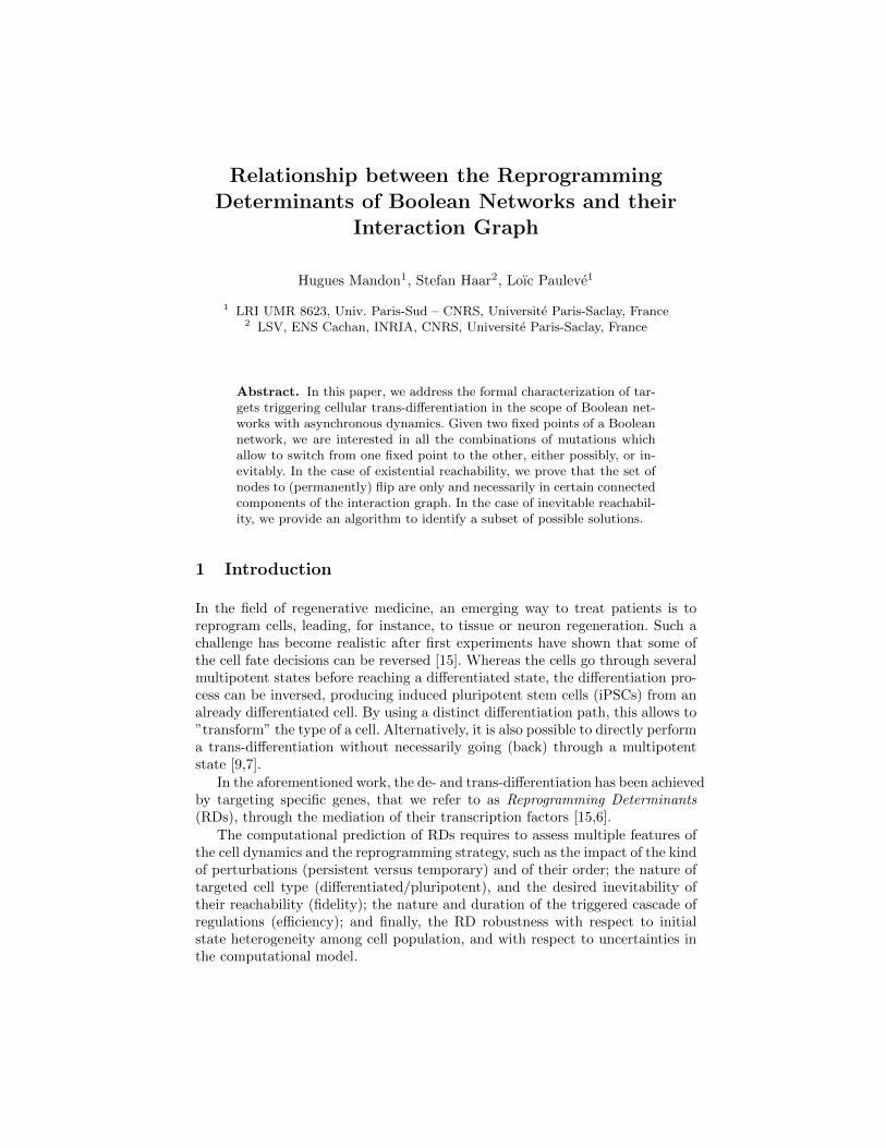
value. If we ”change” u to 1 (resp. 0), then fu(x) = 1 (resp. 0) for all x. Whenswitching to y (by changing I) is possible, we have two cases : it either meansthat y is reachable from x[xI=yI ] (existential reachability, Def. 6), or that y is theonly reachable fixed point from x[xI=yI ] (inevitable reachability, Def. 7). Theseare two different approaches that we will both consider. To remove the temporalaspect, we make all the changes at the same time (hence x[xI=yI ], otherwise anorder should be visible), and only watch if y is reachable. This also means thatthere is no indication of how long it takes for y to be reached.

Definition 6 (Existential Reachability). With the boolean network F, a

function ERF can be defined as ERF : 22[n]

, with ERF (x, y) 7→ v where vis the set of all minimal vertex sets I such that x[xI=yI ] →∗ y.

Definition 7 (Inevitable Reachability). Similarly, a function IRF : 22[n]

can be defined as IRF (x, y) 7→ w where w is the set of all minimal vertices setsI such as ∀z ∈ {0, 1}n, x[xI=yI ] →∗ z ⇒ z →∗ y.

These two functions will give different results, and have different meanings,as shown in the examble below.

Example 3. Let us consider the BN f of Fig.3 and its transition graph repro-duced in Fig.4. f has 4 fixed points: 0000, 0001, 1100 and 1101. Let x = 0000and y = 1100. Fixing the node {1} to 1 in x makes y reachable : 1100 (=y) isreachable from x[x1=1] = 1000 with the Boolean network f ′ defined by f ′1(x) = 1and f ′2 = f2, f ′3 = f3, f ′4 = f4. The transition graph of f ′, considering the firstnode being active, corresponds to the left part of the transition graph in Fig.4.One can then remark that y is not the only fixed point reachable: from 1000,1101 is also reachable. If we also fix the node {4} to 0, y is the only reachablefixed point from x[x1=1,x4=0] in the Boolean network f ′′ such that f ′′1 (x) = 1,f ′′2 = f2, f ′′3 = f3, and f ′′4 (x) = 0.

Therefore, with the previous definitions, {1} ∈ ERF (0000, 1100) but {1} /∈IRF (0000, 1100); and {1, 4} ∈ IRF (0000, 1100) but {1, 4} /∈ ERF (0000, 1100).Moreover, we also have {1, 2} and {1, 3} ∈ IRF (0000, 1100).

f1(x) = x1

f2(x) = x1

f3(x) = x1 ∧ ¬x3

f4(x) = x3 ∨ x4

1

23

4

Fig. 3. A BN of dimension 4

1010 1110

1000x{1} = 1100

y

1011 1111

1001 1101

0010

0000

x

0110

0100

0011 0111

0001 0101

Fig. 4. Transition graph of the BN in Fig.3

4 Reprogramming Determinants and the SCCs of theInteraction Graph

In this section, we show the link between the RDs and the Strongly ConnectedComponents (SCCs) of the interaction graph of the Boolean network f . Ourresults make the assumption that all the attractors of f are fixed points (nocyclic attractors).

4.1 SCC Ordering

To switch from x to y, we want to change the value of each vertex u that hasdifferent values for x and y (xu 6= yu) and to prevent each vertex v that verifiesxv = yv from changing value. We know that changing the value of a vertex canhave an impact on other vertices, but we also know that it will only impact itsdescendants.

So, if a vertex has a different value in x and y but none of its ancestors do,then it is necessary to change this vertex. So, to know which vertices need tobe changed first, the best way is to order them, with a topological order forexample. Of course, if there are loops, an order is impossible to determine, wehave to reduce all SCCs to single ”super-vertices” to achieve it. In the remainingof this paper, we will consider SCCs which contain at least one positive cycle,because they are known to change between fixed points (Theor.1), we call O theSCC set that contains all such SCCs. Reducing the graph to its SCCs makespossible to rank them from 1 to k with any topological order, noted ≺: for alli, j ∈ [k], j > i⇒ Oj 6≺ Oi.

Let C0 be the set {Oi ∈ O | @Oj , Oj ≺ Oi}, and recursively define slicesCK = {Oi ∈ (O \

⋃l∈{1,..,K−1} Cl) | @Oj , Oj ≺ Oi}. Given the definition of

the slices, for all topological orders, the slice set will be the same. The slices arenumbered from 1 to c.

From this order, we know which SCCs need to be impacted, still, SCCs rankedlower in the hierarchy need not be impacted by the change in their ancestors

(see ex.5) The relation ≺ only gives an order to make the changes, from whichone can determine if further changes are needed.

Example 4. Showing that only using the topological order is not sufficient.

f1(x) = ¬x2

f2(x) = ¬x1

f3(x) = x1 ∨ x2

f4(x) = x2 ∧ ¬x3

f5(x) = x4 ∨ x5

3

1 2

4 5

Fig. 5. BN preventing changes in the lower SCC

Any algorithm that only used the topological order without computing thereachable fixed points would not suffice, as the example from Fig.5 shows : theswitch from the fixed point 01100 to 10101 would be computed by just modifying{1}, but in fact {4} will always be fixed at 0, because {4} is always inhibited by{3}, so {5} needs to be changed too.

4.2 SCC Filtering

Whether we want y to be the only reachable attractor, or merely to be oneof potential several such attractors, the ordering from the previous part is thesame, but the filtering will differ.

Theorem 2. If a vertex u such as xu 6= yu and u is not in a positive cycle, thenmodifying u’s ancestors is sufficient to modify u.More generally, to switch from x to y, modifying only those strongly connectedcomponents that contain at least a positive cycle is sufficient.

Proof. Let u be a vertex such that xu 6= yu and u does not lie in a positive cycle.If u is in a negative cycle, the incoming arc from the cycle is irrelevant : giventhat x and y are fixed points and that u has a distinct value in each, the negativecycle does not change u’s value. Given that u is not in a positive cycle, u is not ina SCC (or not relevant if it is in a negative cycle). That means that none of theancestors are descendants of u. Let z be the state where all of Pu (u’s ancestors)have the same value that in y. By the remark from Sect.2, for all v ∈ G[Pu], wehave fv(z) = zv = yv. So, either fu(z) = yu, and the theorem is proven, eitherfu(z) 6= yu, then, by Theor.1, u is in a positive cycle, contradiction. ut

By recursion over the first part, modifying all the SCCs that contain positivecycles so their vertices have the same value as in y modifies all their children,and then all the children of their children, and so on, until the whole graph hasthe same values as y. ut

Selecting the SCCs will differ with the two methods. It relies on the samebase, searching the higher SCC that should have its values modified and that isnot already selected. ”Modified” means that all the values of the SCC are fixedto their values in y. The set of the selected SCCs is S.

4.3 SCC Filtering for Existential Reachability

We consider the RDs for the BN reprogramming with Existential Reachability.We give an algorithm to identify different sets of SCCs for which the mutationin the initial fixed point ensure the reachability of the target fixed point. We willprove that the identified combination of SCCs is complete and minimal.

Basically, the algorithm reviews linearly the SCC slices according to ≺ andadds the minimal combinations of SCCs to S that are different in y and the fixedpoints reachable from x[xS=yS ]:

1. S := ∅2. For i ranging from 1 to c:

– T := ∅– ∀s ∈ P (Ci) such that s minimal∃z ∈ {0, 1}n, zCi\s = yCi\s, x[xI=yI |I∈S] →∗ z, T := T ∪ s.

– S := S×T .

With × being a product and union : for a set I of subsets I1, .., Ik and a setJ1, .., Jl, this product × is defined by : I×J = {I1∪J1, .., I1∪Jl, I2∪J1, ...., Ik∪Jl}

Complexity : In the worst case, the above algorithm perform c× 2l reachabilitychecks (PSPACE-complete [5]), where l is the size of the largest slice.

Existence of a solution and proof of correctness : Forcing all SCCs of such prob-lem that differ on x and y to have the same value as in y is one solution. Inthe worst case, that is what the algorithm will find. Since the algorithm testsreachability, and a solution exists, it will find one.

Example 5. We apply the algorithm on the BN of Fig.6 with x = 00000 andy = 11011.

1. S := ∅2. C1: s minimal ⇔ s = {1}3. S := S×{1} = {{1}}4. C2: s minimal ⇔ s = ∅ 3

5. S := S×∅ = {{1}}.

We now prove the completeness of the algorithm and the minimality of thereturned sets of SCCs (Theorem 3) and that any RDs in ER(x, y) is spans onlyand necessarily in one of the set of SCCs identified by the algorithm (Theorem 4).

3 with the path 10000 → 10100 → 10110 → 11110 → 11111 (and the fixed point isthe next step, → 11011 but there is no need to go further than 11111.)

f1(x) = x1

f2(x) = x1

f3(x) = x1 ∧ ¬x2

f4(x) = x3 ∨ x4

f5(x) = x2 ∨ x5

1

23

4 5

C1

C2

Fig. 6. BN of dimension 5 (left) with its interaction graph (right). Slices are enclosedin boxes. C1 = {{1}}, C2 = {{4}, {5}}.

Theorem 3. S only contains minimal SCC sets, and S is complete.

Proof. Minimality : Inside every slice, the SCCs are totally independant oneanother. Moreover, given the order exploiting, we can deduce that the sum ofthe minima on each slice is the minimum on the whole graph. ut

Completeness : Let I be a minimal SCC set such as x[xJ=yJ |J∈I] →∗ y,then, for every slice Ci, I ∩Ci is minimal, since once all the SCCs in a slice canbe changed to the way they are in y, we can always choose the path that allowsthis change. Hence I ∈ S. ut

Theorem 4. ∀c ∈ ER(x, y), ∃I ∈ S, ∀u ∈ c, ∃scc ∈ I, u ∈ scc.

Proof. Let c be a vertex set in ER(x, y) and u one of the vertices. If u 6∈ O, thenc is not minimal, by Theorem 2. If for all I ∈ S, u is in o ∈ (O \ I) then thereexists a path such that changing o’s ancestors makes o’s change possible, andthe ancestors need to be changed as well, by construction of I. So c \ u wouldhave the same effect, and c would not be minimal. If u 6∈ o, then there existsI ∈ S and scc ∈ I, such as u ∈ scc. ut

4.4 SCC Filtering for Inevitable Reachability

We now give an algorithm to identify a set of SCCs for which the mutation inthe initial fixed point is sufficient to ensure the Inevitable Reachability of thetarget fixed point.

The algorithm computes all reachable fixed points from x with the SCCs inS modified, and find the one, z, that has the lower SCC (in the ranking given by≺) in which a vertex u is such that zu 6= yu. As we are looking for all reachablefixed points, this will always return the same SCC (even if the order is onlypartial), thus allowing the algorithm to be deterministic. We add this SCC toS, and repeat until y is the only reachable fixed point.

1. S := ∅2. While ∃z ∈ FP(f), z 6= y, x[xI=yI |I∈S] →∗ z

– S := S ∪ {Oi}, withi = mina∈{1,..,k}(a | ∃z ∈ FP(f), zOa

6= yOa, x[xI=yI |I∈S] →∗ z)

If two (or more) SCCs A and B are such that they are differently ordered intwo distinct orders, then A has no influence on B and neither has B on A. Then,the algorithm will select both SCCs if neither are impacted by the previouschanges, so the order does not matter.

Existence of a solution and proof of correctness : A solution is to fix all the SCCsof the graph to their value in y. Since there exists a solution and the algorithmtests if y is the only reachable point, and follows the order given by ≺, it willend and find a solution.

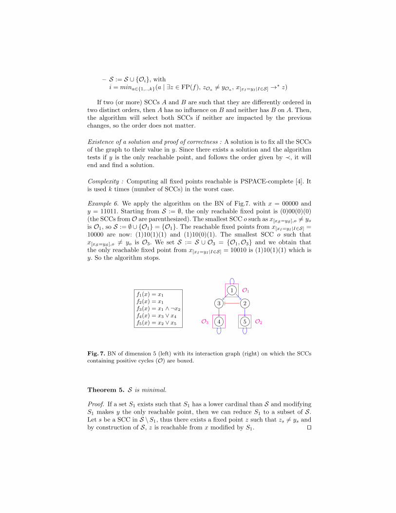
Complexity : Computing all fixed points reachable is PSPACE-complete [4]. Itis used k times (number of SCCs) in the worst case.

Example 6. We apply the algorithm on the BN of Fig.7. with x = 00000 andy = 11011. Starting from S := ∅, the only reachable fixed point is (0)00(0)(0)(the SCCs fromO are parenthesized). The smallest SCC o such as x[xS=yS ],o 6= yois O1, so S := ∅ ∪ {O1} = {O1}. The reachable fixed points from x[xI=yI |I∈S] =10000 are now: (1)10(1)(1) and (1)10(0)(1). The smallest SCC o such thatx[xS=yS ],o 6= yo is O3. We set S := S ∪ O3 = {O1,O3} and we obtain thatthe only reachable fixed point from x[xI=yI |I∈S] = 10010 is (1)10(1)(1) which isy. So the algorithm stops.

f1(x) = x1

f2(x) = x1

f3(x) = x1 ∧ ¬x2

f4(x) = x3 ∨ x4

f5(x) = x2 ∨ x5

1

23

4 5

O1

O3 O2

Fig. 7. BN of dimension 5 (left) with its interaction graph (right) on which the SCCscontaining positive cycles (O) are boxed.

Theorem 5. S is minimal.

Proof. If a set S1 exists such that S1 has a lower cardinal than S and modifyingS1 makes y the only reachable point, then we can reduce S1 to a subset of S.Let s be a SCC in S \S1, thus there exists a fixed point z such that zs 6= ys andby construction of S, z is reachable from x modified by S1. ut

We remark that, contrary to the case of Existential Reachability, the RDsfor Inevitable Reachability of the target fixed point are not necessarily in SCCscontaining positive cycles. Indeed, in Ex.3, we showed that IRF (x, y) can referto nodes that do not belong to O (such as the node 2 for the BN of Fig.3). Butwe can also remark that if a RD v is not in a SCC containing a positive cycle,then xv = yv.

Theorem 6. ∀v ∈ IR(x, y), xv 6= yv ⇒ ∃scc ∈ O, v ∈ scc

Proof. Let v ∈ IR(x, y) such that for all scc ∈ O, v 6∈ scc. By Theor.1, if v issuch that xv 6= yv, then modifying the SCC in O is enough to modify v. Butv ∈ IR(x, y) and IR(x, y) is minimal, thus xv = yv. ut

5 Identifying Determinants within SCCs

We know that modifying all the SCCs selected is enough to switch from x toy, but to reduce the genes selected, we could try to modify only some of thevertices to achieve the same result. But, as dynamics are involved, there couldbe unwanted changes (or wanted and unpredicted changes, in the case where wewant y to be reachable) in the descendants.

An idea could be to select the feedback vertex set of the SCC : by fixing thevertices from this set, we effectively destroy every circle, thus the only reachablestate of the SCC is the one having the same values as y. This, however, doesnot solve the problem : in Ex.7, {1} is the feedback vertex set, and we still havethe same issue. Moreover, it miss some of the possible solutions (modifying {2}or {3} could work to change the whole SCC in Ex.7) or even dismiss the bestsolution (in Ex.7, changing {3} makes y the only reachable fixed point and solvesthe issue).

Example 7. Illustration of the problem with dynamics.

f1(x) = ¬x3 ∧ ¬x2

f2(x) = ¬x1

f3(x) = ¬x1

f4(x) = x2 ∧ ¬x1 ∧ ¬x3

f5(x) = x4 ∨ x5

1

2

3

4 5

Fig. 8. BN of dimension 5 (left) and its interaction graph (right)

We decide that x = 10000 and y = 01100, and 01101 = z, those are allfixed points. Let’s suppose we want y to be the only fixed point reachable.The algorithm will see that if the whole first SCC is modified {1, 2, 3}, y is

the only reachable fixed point. It could pick {1} to be modified, but instead of00000→ 00100→ 01100, we can have

00000→ 01000→ 01010→ 01011→ 01111→ 01101

This leads to z being reachable by only modifying {1}, and so the algorithmwould be wrong.

This leaves to two kinds of approaches : either a way to modify the SCC sothat it does not impact its descendants can be found, either we need to selectthe vertices to be modified in the SCC as a intermediary step in the process,and redesign S as a list of vertices instead of a list of SCCs.

By exploiting the results of the preceding section, we show an algorithm tocompute a set of RDs which guarantees the Inevitable Reachability of the targetfixed point. The algorithm recursively picks a vertex u in the lowest SCC inthe order given by ≺ in O, and modify its associated function to become theconstant value yu. The interaction graph of the resulting Boolean network is asub-graph of the initial interaction graph, where all the input edges of the nodeu have been removed. Hence, the SCC O1 is split in the new interaction graph. Ifnecessary, another vertex can be picked in the lowest SCC in the new interactiongraph:

RecursiveAlgorithm(f , rd) :

– If ∃z ∈ FP(f), x[xrd=yrd] →∗ z then :

• res = ∅• i = mina∈{1,..,k}(a | ∃z ∈ FP(f), zOa 6= yOa , x[xI=yI |I∈S] →∗ z)

• For all u ∈ Oi :

∗ g := f with gu := yu∗ res := res∪ RecursiveAlgorithm(g, rd×{u})

• return res

– else :

• return rd

Remark that the algorithm always find at least one solution: if the target fixedpoint is not the only reachable fixed point, then there is at least one positivecycle (and hence a SCC) which has a different state (and hence will be selectedby our algorithm).

Example 8. Applied to the BN of Fig.8 with x = 10000 and y = 01100, theabove algorithm returns, for instance, the RD {2, 5}: indeed, {2} belongs toO1. When fixing f2 = 1, the new interaction graph has two SCCs with positivecycles: {1, 3} and {5}. From the state 11000, two fixed points are reachable:01100, 01101. Hence, because the SCC {1, 3} has the same values than in y inthose two fixed points, the next vertex in picked in the SCC {5}. Finally, fromthe state 11001, y is the only reachable fixed point.

6 Discussion

This paper provides the first formal characterization of the Reprogramming De-terminants (RDs) for switching from one fixed point to another in the scope ofthe asynchronous dynamics of Boolean networks.

In the case of reprogramming with existential reachability of the target fixedpoint, we prove that all the possible minimal RDs modify nodes in particu-lar combinations of SCCs of the interaction graph of the Boolean network. Wegive an algorithm to determine exactly those combinations of set of nodes. Ourcharacterizations rely on the verification of reachability properties.

In the case of reprogramming with inevitable reachability of the target fixedpoint, we show that the RDs are not necessarily in SCCs. However, we providean algorithm which identifies RDs that guarantee the inevitable reachability bypicking nodes in appropriate SCCs. The algorithm relies on the enumeration ofreachable fixed points.

One of the main limitation of our algorithms is the numerous reachabilitychecks it needs to perform. Future work will consider methods and data struc-tures for factorizing the exploration of the Boolean network dynamics.

The present work considered only permanent mutations: when a node ismutated, it is assumed it keeps its mutated value forever (its local Booleanfunction becomes a constant function). Considering temporary mutations, i.e.,where the local Boolean function of mutated nodes is restored after some time,is a challenging research direction: one should determine the ordering and theduration of mutations, and the set of candidate mutations is a priori no longerrestricted to connected components, as it is the case for permanent mutations.

References

1. Wassim Abou-Jaoude, Pedro T. Monteiro, Aurelien Naldi, Maximilien Grand-claudon, Vassili Soumelis, Claudine Chaouiya, and Denis Thieffry. Model checkingto assess t-helper cell plasticity. Frontiers in Bioengineering and Biotechnology, 2,2015.

2. Julio Aracena. Maximum number of fixed points in regulatory boolean networks.Bulletin of Mathematical Biology, 70(5):1398–1409, feb 2008.

3. Rui Chang, Robert Shoemaker, and Wei Wang. Systematic search for recipesto generate induced pluripotent stem cells. PLoS Computational Biology,7(12):e1002300, Dec 2011.

4. Thomas Chatain, Stefan Haar, Loıg Jezequel, Loıc Pauleve, and Stefan Schwoon.Characterization of reachable attractors using Petri net unfoldings. In PedroMendes, Joseph Dada, and Kieran Smallbone, editors, Computational Methodsin Systems Biology, volume 8859 of Lecture Notes in Computer Science, pages129–142. Springer Berlin Heidelberg, 2014.

5. Allan Cheng, Javier Esparza, and Jens Palsberg. Complexity results for 1-safenets. Theor. Comput. Sci., 147(1&2):117–136, 1995.

6. Isaac Crespo, Thanneer M Perumal, Wiktor Jurkowski, and Antonio del Sol. De-tecting cellular reprogramming determinants by differential stability analysis ofgene regulatory networks. BMC Systems Biology, 7(1):140, 2013.

7. Antonio del Sol and Noel J. Buckley. Concise review: A population shift view ofcellular reprogramming. STEM CELLS, 32(6):1367–1372, 2014.

8. Zuguang Gao, Xudong Chen, and Tamer Basar. On the stability of conjunctiveboolean networks. March 2016.

9. Thomas Graf and Tariq Enver. Forcing cells to change lineages. Nature,462(7273):587–594, dec 2009.

10. Junghyun Jo, Sohyun Hwang, Hyung Joon Kim, Soomin Hong, Jeoung Eun Lee,Sung-Geum Lee, Ahmi Baek, Heonjong Han, Jin Il Lee, Insuk Lee, and et al. Anintegrated systems biology approach identifies positive cofactor 4 as a factor thatincreases reprogramming efficiency. Nucleic Acids Research, 44(3):1203–1215, Jan2016.

11. Loıc Pauleve. Goal-oriented reduction of automata networks. In CMSB 2016 -14th conference on Computational Methods for Systems Biology, 2016. accepted.

12. Owen J L Rackham, Jaber Firas, Hai Fang, Matt E Oates, Melissa L Holmes,Anja S Knaupp, Harukazu Suzuki, Christian M Nefzger, Carsten O Daub, Jay WShin, Enrico Petretto, Alistair R R Forrest, Yoshihide Hayashizaki, Jose M Polo,and Julian Gough. A predictive computational framework for direct reprogram-ming between human cell types. Nature Genetics, 48(3):331–335, jan 2016.

13. Adrien Richard. Positive circuits and maximal number of fixed points in discretedynamical systems. Discrete Applied Mathematics, 157(15):3281 – 3288, 2009.

14. Adrien Richard. Negative circuits and sustained oscillations in asynchronous au-tomata networks. Advances in Applied Mathematics, 44(4):378 – 392, 2010.

15. Kazutoshi Takahashi and Shinya Yamanaka. A decade of transcription factor-mediated reprogramming to pluripotency. Nat Rev Mol Cell Biol, 17(3):183–193,Feb 2016.

16. Rene Thomas. Boolean formalization of genetic control circuits. Journal of Theo-retical Biology, 42(3):563 – 585, 1973.

17. Elisabeth Remy, Paul Ruet, and Denis Thieffry. Graphic requirements for mul-tistability and attractive cycles in a boolean dynamical framework. Advances inApplied Mathematics, 41(3):335 – 350, 2008.