RELATIONS IN THE WITT GROUP OF NONDEGENERATE

BRAIDED FUSION CATEGORIES ARISING FROM THE

REPRESENTATION THEORY OF QUANTUM GROUPS

AT ROOTS OF UNITY

by

ANDREW P. SCHOPIERAY

A DISSERTATION

Presented to the Department of Mathematicsand the Graduate School of the University of Oregon

in partial fulfillment of the requirementsfor the degree of

Doctor of Philosophy

June 2017

DISSERTATION APPROVAL PAGE

Student: Andrew P. Schopieray

Title: Relations in the Witt Group of Nondegenerate Braided Fusion CategoriesArising from the Representation Theory of Quantum Groups at Roots of Unity

This dissertation has been accepted and approved in partial fulfillment of therequirements for the Doctor of Philosophy degree in the Department ofMathematics by:

Victor Ostrik ChairArkady Berenstein Core MemberAlexander Kleshchev Core MemberAlexander Polishchuk Core MemberDietrich Belitz Institutional Representative

and

Scott Pratt Dean of the Graduate School

Original approval signatures are on file with the University of Oregon GraduateSchool.

Degree awarded June 2017

ii

c© 2017 Andrew P. Schopieray

iii

DISSERTATION ABSTRACT

Andrew P. Schopieray

Doctor of Philosophy

Department of Mathematics

June 2017

Title: Relations in the Witt Group of Nondegenerate Braided Fusion CategoriesArising from the Representation Theory of Quantum Groups at Roots of Unity

For each finite dimensional Lie algebra g and positive integer k there exists a

modular tensor category C(g, k) consisting of highest weight integrable g-modules

of level k where g is the corresponding affine Lie algebra. Relations between the

classes [C(sl2, k)] in the Witt group of nondegenerate braided fusion categories

have been completely described in the work of Davydov, Nikshych, and Ostrik.

Here we give a complete classification of relations between the classes [C(sl3, k)]

relying on the classification of conncted etale alegbras in C(sl3, k) (SU(3) modular

invariants) given by Gannon. We then give an upper bound on the levels for

which exceptional connected etale algebras may exist in the remaining rank 2

cases (C(so5, k) and C(g2, k)) in hopes of a future classification of Witt group

relations among the classes [C(so5, k)] and [C(g2, k)]. This dissertation contains

previously published material.

iv

CURRICULUM VITAE

NAME OF AUTHOR: Andrew P. Schopieray

GRADUATE AND UNDERGRADUATE SCHOOLS ATTENDED:

University of Oregon, Eugene, Oregon

Western Washington University, Bellingham, Washington

Grand Valley State University, Allendale, Michigan

Northwestern Michigan College, Traverse City, Michigan

DEGREES AWARDED:

Doctor of Philosophy, Mathematics, 2017, University of Oregon

Master of Science, Mathematics, 2012, Western Washington University

Bachelor of Science, Mathematics, 2010, Grand Valley State University

Associate of Applied Science, 2007, Northwestern Michigan College

AREAS OF SPECIAL INTEREST:

Quantum Algebra

Representation Theory

PROFESSIONAL EXPERIENCE:

Graduate Teaching Fellow, Department of Mathematics, University ofOregon, 2012–2017

Instructor, University of Oregon Center for Youth Enrichment/Talentedand Gifted Education, 2013–2015

Instructor, Whatcom Community College, 2011–2012

Graduate Teaching Assistant, Western Washington University, 2010–2012

PUBLICATIONS:

Andrew Schopieray. Classification of sl3 relations in the Witt group ofnondegenerate braided fusion categories. Communications in MathematicalPhysics, 353(3):1103–1127, 2017

Andrew Schopieray. Level bounds for exceptional quantum subgroups inrank two. submitted for publication, 2017

v

ACKNOWLEDGEMENTS

There are too many people who deserve recognition for their contributions

in my life up to this point, so I will mention only those major characters who

haven’t been acknowledged previously in print, and had a substantial role in my

intellectual upbringing. Most likely you will all be thanked in future publications

that will have higher readership.

The lion’s share of gratitude for my research is owed to my advisor, Victor

Ostrik. Despite how little credit he would willfully claim for my successes, Victor

has served as a source of inspiration and leadership since we met and burned

through Humphreys in the winter of 2014. Every established researcher I have

met in this field has a similar respect and gratitude, and I consider myself very

privileged to call myself his student.

Next in the reverse chronological order of thanks comes Matt Boelkins who, in

2009, informed an ungrateful and misguided undergraduate student that mathe-

matics can be a career. For that he will have to deal with me thanking him ad

infinitum.

While I was still cooking professionally 12-hours each day, Jim Valovick showed

me that open-mindedness and compassion are fundamental to the human expe-

rience. He would go on to teach me philosophy, religion, and Latin, before his

passing in 2007. It’s with tears in my eyes that I yet again thank him indirectly,

having not matured enough to be able to tell him face-to-face when I had the

chance.

Lastly my thanks go to Cheney, who everyone already knows, because like a

little boy I still go on and on about “how cool my big brother is”. Dings and dents

included, you’ll always be the spitting image of what I aspire to achieve.

vi

TABLE OF CONTENTS

Chapter Page

I. INTRODUCTION . . . . . . . . . . . . . . . . . . . . . . . . . . . . . . 1

II. PRELIMINARIES . . . . . . . . . . . . . . . . . . . . . . . . . . . . . . 4

2.1. Fusion Subcategories and Prime Decomposition . . . . . . . . . . . 6

2.2. Modular Categories . . . . . . . . . . . . . . . . . . . . . . . . . . . 7

2.3. Etale Algebras . . . . . . . . . . . . . . . . . . . . . . . . . . . . . . 9

2.4. The Witt Group of Nondegenerate Braided Fusion Categories . . . 11

III.QUANTUM GROUPS TO MODULAR TENSOR CATEGORIES . . . . 13

3.1. Numerical Data and Fusion Rules for C(g, k) when rank(g) ≤ 2 . . . 15

3.2. C(sl3, k) . . . . . . . . . . . . . . . . . . . . . . . . . . . . . . . . . 22

3.2.1. Fusion Subcategories of C(sl3, k) . . . . . . . . . . . . . . . . 23

3.2.2. Prime Decomposition when 3 - k . . . . . . . . . . . . . . . . 24

3.2.3. Simplicity of C(sl3, k)0A when 3 | k . . . . . . . . . . . . . . . 27

IV.WITT GROUP RELATIONS . . . . . . . . . . . . . . . . . . . . . . . . 34

4.1. Modular Invariants and Conformal Embeddings . . . . . . . . . . . 34

4.2. A Classification of sl3 Relations . . . . . . . . . . . . . . . . . . . . 38

V. CONNECTED ETALE ALGEBRAS IN C(g, k) . . . . . . . . . . . . . . 43

5.1. Technical Machinery . . . . . . . . . . . . . . . . . . . . . . . . . . 43

5.2. Exceptional Algebras . . . . . . . . . . . . . . . . . . . . . . . . . . 48

5.3. Proof of Theorem 5: C(so5, k) . . . . . . . . . . . . . . . . . . . . . 52

5.3.1. The Case m = 0 and 0 < ` < k − 1 . . . . . . . . . . . . . . 53

5.3.2. The Case 2 ≤ m ≤ x+ 2 . . . . . . . . . . . . . . . . . . . . 55

5.3.3. The Case ` = 0 and m < k . . . . . . . . . . . . . . . . . . . 57

5.3.4. The Case 0 6= ` ≤ x < m− 2 . . . . . . . . . . . . . . . . . . 58

5.4. Proof of Theorem 5: C(g2, k) . . . . . . . . . . . . . . . . . . . . . . 61

5.4.1. The Case 0 ≤ ` ≤ 2 . . . . . . . . . . . . . . . . . . . . . . . 62

5.4.2. The Case m = 0 . . . . . . . . . . . . . . . . . . . . . . . . . 65

5.4.3. The Case 3 ≤ ` ≤ x+ 3 . . . . . . . . . . . . . . . . . . . . 66

5.4.4. The Case x+ 3 < ` and m 6= 0 . . . . . . . . . . . . . . . . 69

REFERENCES CITED . . . . . . . . . . . . . . . . . . . . . . . . . . . . . 72

vii

LIST OF FIGURES

Figure Page

1. Roots of unity q when rank(g) ≤ 2 . . . . . . . . . . . . . . . . . . . . 13

2. Modulus of qm − q−m . . . . . . . . . . . . . . . . . . . . . . . . . . . . 14

3. C(sl2, 6) . . . . . . . . . . . . . . . . . . . . . . . . . . . . . . . . . . . 15

4. C(sl3, 4) . . . . . . . . . . . . . . . . . . . . . . . . . . . . . . . . . . . 16

5. C(so5, 6) . . . . . . . . . . . . . . . . . . . . . . . . . . . . . . . . . . . 17

6. C(g2, 8) . . . . . . . . . . . . . . . . . . . . . . . . . . . . . . . . . . . 18

7. λ⊗ γ ∈ C(so5, 12) . . . . . . . . . . . . . . . . . . . . . . . . . . . . . . 21

8. Adjacent vs. nonadjacent to Ti (level k = 5) . . . . . . . . . . . . . . . 24

9. C0A at level k = 6 and the action of a corner weight . . . . . . . . . . . 27

10. (3, 4)⊗ (4, 3) ∈ C(sl3, 12) . . . . . . . . . . . . . . . . . . . . . . . . . . 51

11. Possible (`,m) when k = 14 and x = 5 . . . . . . . . . . . . . . . . . . 53

12. (6, 0)⊗ (7, 0) ∈ C(so5, 9) . . . . . . . . . . . . . . . . . . . . . . . . . . 54

13. (6, 0)⊗ (7, 4) ∈ C(so5, 12) . . . . . . . . . . . . . . . . . . . . . . . . . 56

14. (0, 10)⊗ (0, 10) ∈ C(so5, 11) . . . . . . . . . . . . . . . . . . . . . . . . 57

15. (0, 6)⊗ (3, 7) ∈ C(so5, 10) . . . . . . . . . . . . . . . . . . . . . . . . . 59

16. Possible (`,m) when k = 20 and x = 5 . . . . . . . . . . . . . . . . . . 62

17. (0, 5)⊗ (0, 6) ∈ C(g2, 18) . . . . . . . . . . . . . . . . . . . . . . . . . . 63

18. (9, 0)⊗ (15, 0) ∈ C(g2, 20) . . . . . . . . . . . . . . . . . . . . . . . . . 65

19. (0, 4)⊗ (3, 4) ∈ C(g2, 15) . . . . . . . . . . . . . . . . . . . . . . . . . . 67

20. (12, 0)⊗ (14, 4) ∈ C(g2, 24) . . . . . . . . . . . . . . . . . . . . . . . . . 70

viii

CHAPTER I

INTRODUCTION

This dissertation is a compilation of two existing articles. Chapters II and IV

have appeared in [41] (the final publication is available at Springer via

http://dx.doi.org/10.1007/s00220-017-2831-z), Chapter V has appeared in

[42] which has been submitted for publication, and Chapters I and III include

overlapping portions of both [41] and [42].

The Witt group of nondegenerate braided fusion categoriesW , first introduced

in [10], provides an algebraic structure that is one tool for organizing braided

fusion categories. Inside W lies the subgroup Wun consisting of classes of pseudo-

unitary braided fusion categories which, in turn, contains the classes [C(g, k)]

coming from the representation theory of affine Lie algebras. Theorem 3 is the

main goal of this exposition, to classify all relations in the Witt group between

the classes [C(sl3, k)]. To do so requires identification of a unique (up to braided

equivalence) representative of each Witt equivalence class which is simple and

completely anisotropic (see Definitions 3 and 8), constructed in the cases where

3 | k as the category of dyslectic A-modules C(sl3, k)0A [27, Definition 1.8]. The

major result which allows for the classification is Theorem 1 which states that the

categories C(sl3, k)0A are simple when 3 | k and k 6= 3.

Translated into the language of modular tensor categories, there is a common

belief among physicists [30] that Wun is generated by the classes of the categories

C(g, k). This provides at least one external motivation for understanding Witt

group relations in Wun. But Witt group relations are difficult to come by; all

relations in the subgroupWpt ⊂ W consisting of pointed braided fusion categories

are known [14, Appendix A.7] and limited relations in Wun are known due to the

theory of conformal embeddings of vertex operator algebras (Section 4.1.). The

1

general task of classifying all relations inWun was presented in [10], and in [11] all

relations among the classes of the categories C(sl2, k) were classified. Independent

from the classification of Witt group relations, the passage from [C] ∈ Wun to

[C0A], the equivalence class of the category of dyslectic A-modules over a connected

etale algebra, is intimately related to extensions of vertex operator algebras [24]

and anyon condensation [21] (see also [15, 29]), providing stronger justification

to conjecture and prove results similar to Theorem 3 for general C(g, k). If these

results are true they also provide an infinite collection of simple modular tensor

categories which play an important role in the classification of all modular tensor

categories, an open and active area of modern research.

Modular tensor categories also encode the data of chiral conformal field theo-

ries. Fuchs, Runkel, and Schweigert [19] describe how full conformal field theories

correspond to certain commutative algebras in these categories. These concepts

have been recently formalized to logarithmic conformal field theories [20], i.e. theo-

ries described by non-semisimple analogs of modular tensor categories. One should

also refer to the work of Bockenhauer, Evans, and Kawahigashi [4, 5] which de-

scribes this connection in terms of modular invariants and subfactor theory, or

Ostrik’s summary of these results in categorical terms [35, Section 5].

Lastly, the aforementioned connected etale algebras partially classify module

categories over fusion categories. Each connected etale algebra A ∈ C gives rise to

an indecomposable module category over C by considering CA, the category of A-

modules in C, although not all indecomposable module categories can be produced

in this way. For example if C is a pointed modular tensor category [17, Chapter

8.4] with the set of isomorphism classes of simple objects of C forming a finite

abelian group G, then indecomposable module categories over C correspond to

subgroups of G along with additional cohomological data [34, Theorem 3.1]; this

example provides some precedence to title connected etale algebras as quantum

subgroups. For a non-modular example, module categories over the even parts of

the Haagerup subfactors have been classified by Grossman and Snyder [23]. More

2

classically, module categories over C(sl2, k) are classified by simply-laced Dynkin

diagrams [7, 27] but this characterization scheme has not immediately lent itself

to classifying module categories over C(g, k) for other simple Lie algebras g. The

language and tools of tensor categories which have solidified in recent years provide

a novel approach to this dated problem.

There is a long-standing belief that the modular tensor categories C(g, k) con-

tain exceptional (see Section 5.2.) connected etale algebras at only finitely many

levels k. Here in Theorem 5 we confirm this conjecture when g = so5, g2, con-

tributing a proof and explicit bounds, adding to the previously known positive

results for sl2 [27] and sl3 [22]. The explicit level-bound provided optimistically

allows for a complete classification of connected etale algebras in C(so5, k) and

C(g2, k) by strictly computational methods.

3

CHAPTER II

PRELIMINARIES

Chapter II appeared in [41] (the final publication is available at Springer via

http://dx.doi.org/10.1007/s00220-017-2831-z).

We assume familiarity with the basic definitions and results found for example

in [17], but will give a brief recollection at this point. In the remainder of this

section k will be an algebraically closed field of characteristic zero.

A fusion category over k is a k-linear semisimple rigid tensor category with

finitely many isomorphism classes of simple objects, finite dimensional spaces of

morphisms, and a simple unit object 1. For brevity, the set of isomorphism classes

of simple objects of a fusion category C will be denoted O(C). We will identify

the unique (up to tensor equivalence) fusion category with one simple object with

Vec, the category of finite dimensional vector spaces over k. Given two braided

fusion categories C and D, Deligne’s tensor product C�D is a new braided fusion

category which can be realized as the completion of the k-linear direct product

C ⊗k D under direct sums and subobjects under our current assumptions [17,

Section 4.6].

A set of natural isomorphisms

cX,Y : X ⊗ Y ∼−→ Y ⊗X (1)

satisfying compatibility relations [17, Section 8.1] for all X, Y in a fusion category

C is called a braiding on C and we will therefore refer to C as a braided fusion

category. There is an alternative reverse braiding for any braided category given

by cX,Y := c−1Y,X and the resulting braided category is denoted Crev.

Example 1 (Pointed fusion categories). Special distinction goes to fusion

4

categories C in which every object X ∈ O(C) is invertible, i.e. the evaluation

evX : X∗ ⊗ X −→ 1 and coevaluation coevX : 1 −→ X ⊗ X∗ maps coming

from the rigidity of C are isomorphisms. Categories in which every X ∈ O(C) is

invertible are called pointed, while the maximal pointed subcategory of a braided

fusion category C will be denoted Cpt. Pointed braided fusion categories were

classified by Joyal and Street in [26, Section 3] (see also [17, Section 8.4]). If a

pointed fusion category is braided, due to (1) the set of isomorphism classes of

simple objects forms a finite abelian group under the tensor product, which we

will call A. Recall that a quadratic form on A with values in k× is a function

q : A → k× such that q(−x) = q(x) and b(x, y) = q(x + y)/(q(x)q(y)) is bilinear

for all x, y ∈ A. To each pair (A, q) there exists a braided fusion category C(A, q)

that is unique up to braided equivalence whose simple objects are labelled by the

elements of A.

One might identify symmetric braidings (those for which cY,X ◦ cX,Y = idX⊗Y )

as the most elementary of braidings as Deligne [12][13][17, Section 9.9] proved that

all symmetric fusion categories must come from the representation theory of finite

groups. In the spirit of gauging how far a braiding is from being symmetric, if

cY,X ◦ cX,Y = idX⊗Y for any objects X, Y ∈ C, we say X and Y centralize one

another [32, Section 2.2].

Definition 1. If D is a subcategory of a braided fusion category C that is closed

under tensor products then D′ ⊂ C the centralizer of D in C is the full subcategory

of objects of C that centralize each object of D. A braided fusion category is known

as nondegenerate if C ′ ' Vec.

Note 1. One can think of nondegenerate braided fusion categories as those which

are furthest from symmetric as possible.

Example 2 (Metric groups). If the symmetric bilinear form b(−,−) associated

with a pair (A, q) (as in Example 1) is nondegenerate, then the pair (A, q) is called

a metric group. It is known [17, Example 8.13.5] that the category C(A, q) is

5

nondegenerate if and only if (A, q) is a metric group. For instance let A := Z/3Z

(considered as the set {0, 1, 2} with the operation of addition modulo 3). The

following functions are quadratic forms on A with values in C×:

qω :A −→ C× qω2 :A −→ C×

x 7→ (ω)x2

x 7→ (ω2)x2

where ω = exp(2πi/3). These quadratic forms equip C(Z/3Z, qω) and

C(Z/3Z, qω2) with the structure of nondegenerate braided fusion categories which

are not braided equivalent.

2.1. Fusion Subcategories and Prime Decomposition

The assumptions required of a fusion subcategory are very few in number.

Definition 2. A full subcategory D of a fusion category C is a fusion subcategory

if D is closed under tensor products.

It would not be unreasonable to assume that rigidity and existence of the unit

object of D be required in the definition above, but both are consequences of

closure under tensor products. Specifically Lemma 4.11.3 of [17] gives that for

each simple object X there exists n ∈ Z>0 such that Hom(1, X⊗n) 6= 0. And

by adjointness of duality [17, Proposition 2.10.8] Hom(X∗, X⊗(n−1)) 6= 0 as well.

Thus 1, X∗ ∈ C are direct summands of sufficiently large tensor powers of X.

Definition 3. A fusion category with no proper, nontrivial fusion subcategories

is called simple, while a nondegenerate fusion category with no proper, nontrivial,

nondegenerate fusion subcategories is called prime.

The existence of a decomposition of a nondegenerate braided fusion category

into a product of prime fusion subcategories was given by Muger [32, Section 4.1]

6

under limited assumptions and proved in the following generality in Theorem 3.13

of [14].

Proposition 1. Let C 6= Vec be a nondegenerate braided fusion category. Then

C ' C1 � · · ·� Cn,

where C1, . . . , Cn are prime nondegenerate subcategories of C.

To construct such a decomposition one can identify a nontrivial nondegener-

ate braided fusion subcategory D inside of a given nondegenerate braided fusion

category C and by Theorem 4.2 of [32], C ' D � D′ is a braided equivalence.

In future sections this process will be referred to as Muger’s decomposition. As

noted in [32, Remark 4.6] this decomposition is not necessarily unique which is a

significant observation for the discussion in Section 2.4..

2.2. Modular Categories

Recall the natural isomorphisms aV : V∼−→ V ∗∗ for any finite dimensional

vector space V over k from elementary linear algebra. This collection of natural

isomorphisms is a pivotal structure on Vec, i.e. they satisfy aV⊗W = aV ⊗ aW for

any finite dimensional vector spaces V and W . A pivotal structure on a general

tensor category C allows us to define a categorical analog of trace, Tr(f) ∈ k for

any morphism f ∈ End(X) [17, Section 4.7] given by

Tr(f) : 1coevX−→ X ⊗X∗ aX◦f⊗idX∗−→ X∗∗ ⊗X∗ evX∗−→ 1.

Tensor categories with a pivotal structure aX : X∼−→ X∗∗ for all objects X will

be called pivotal themselves.

Definition 4. The (categorical or quantum) dimension of an object X in a pivotal

tensor category C is dim(X) := Tr(idX) ∈ k. A pivotal structure on a tensor

7

category is called spherical if dim(X) = dim(X∗) for all X ∈ O(C), while spherical

braided fusion categories are called pre-modular. One can define the dimension of

a pre-modular category by

dim(C) :=∑

X∈O(C)

dim(X)2.

Example 3 (Vector spaces). There is only one simple object in Vec up to iso-

morphism, the one-dimensional k-vector space 1, and the aforementioned pivotal

structure aV : V∼−→ V ∗∗ given by v 7→ {f 7→ f(v)} is spherical. It is easily

verified that dim(1) = 1 and because the categorical notion of dimension is addi-

tive, then in this case the categorical dimension matches the usual notion of the

dimension of a k-vector space.

More generally the categories C(A, q) are pointed, and so the evaluation, coeval-

uation, and spherical structure can be realized by identity maps. So dim(X) = 1

for all X ∈ O(C(A, q)) and all metric groups (A, q). Moreover dim(C(A, q)) = |A|.

There is a second notion of dimension defined in terms of the Grothendieck

ring K(C) of a fusion category C. As noted in Section 3.3 of [17], there exists

a unique ring homomorphism FPdim : K(C) −→ R such that FPdim(X) > 0

for any 0 6= X ∈ C. This Frobenius-Perron dimension gives an analog to the

dimension of the category C itself as in Definition 4, given by

FPdim(C) :=∑

X∈O(C)

FPdim(X)2.

Spherical fusion categories for which FPdim(C) = dim(C) are called pseudo-

unitary and it is known that for such a category there exists a unique spherical

structure with FPdim(X) = dim(X) for all X ∈ O(C), allowing us to only consider

dim(X) in these cases. It will be important to future computations that dim(X) >

0 for pseudo-unitary fusion categories.

If a braided fusion category is equipped with a spherical structure, there exist

8

natural isomorphisms θX : X∼−→ X for all X ∈ C known as twists (or the ribbon

structure) compatible with the braiding isomorphisms found in (1) of Section II

[17, Section 8.10]. In the case of pointed fusion categories C(A, q) (Example 1),

for any x ∈ A the map θx = b(x, x)idx defines a ribbon structure. The diagonal

matrix consisting of the twists θX over all X ∈ O(C) is called the T -matrix of C.

Finally we end this subsection by tying the notions of trace and dimension

in spherical categories to the nondegeneracy conditions defined by the centralizer

construction (Definition 1).

Definition 5. The S-matrix of a pre-modular category C is the matrix

(sX,Y )X,Y ∈O(C) where sX,Y := Tr(cY,X ◦ cX,Y ). A pre-modular category is modular

if the determinant of its S-matrix is nonzero.

Note 2. It is well-known that a pre-modular category C is modular if and only if

it is nondegenerate (C ′ = Vec). [14, Proposition 3.7][32]

2.3. Etale Algebras

For this exposition, an algebra A in a fusion category C is an associative algebra

with unit which is equipped with a multiplication map m : A ⊗ A −→ A. If m

splits as a morphism of A-bimodules, we refer to A as separable. This criterion

ensures that CA, the category of right A-modules is semisimple, and also A C, A CA,

the categories of left A-modules and A-bimodules respectively [10, Proposition

2.7].

Definition 6. An algebra A in a fusion category C is etale if it is both commutative

and separable. This algebra is connected if dimk Hom(1, A) = 1.

Note 3. Etale algebras have also been referred to as condensable algebras in

the physics literature. The following description of the categories CA when A is

connected etale is summarized from Sections 3.3 and 3.5 of [10].

Braidings on C give rise to functors G : CA −→ CA A defined as M 7→M− (the

identity map as right A-modules), where the left A-module structure on M− is

9

given as composition of the reverse braiding with the right A-module structure

map ρ:

A⊗McM,A−→M ⊗ A ρ−→M.

The commutativity of A implies CA A is a tensor category and thus the above

functor G provides a tensor structure for CA which we denote ⊗A. One can also

define a tensor structure, opposite to the one above, on CA by composing the right

A-module structure map with the usual braiding. We will denote the resulting

left A-module produced from M as M+.

With the tensor structure defined on CA by the functor G, the free module

functor F : C → CA is a tensor functor. In particular F (1) = A is the unit object

of CA which is simple by the assumption that A is connected. The category CA is

also rigid since any object M ∈ CA is a direct summand of the rigid object

F (M) = M ⊗ A = M ⊗A (A⊗ A).

The above discussion implies CA is a fusion category when A ∈ C is connected

etale. Unfortunately the category CA is not braided in general. The issue lies

in the inherent choice of a left A-module structure on a given right A-module

M ∈ CA .

Definition 7. If idM : M− −→M+ is an isomorphism of A-bimodules for M ∈ CA ,

we say that M is dyslectic (also called local in the literature).

Pareigis [37] originally studied the full subcategory of CA consisting of dyslectic

A-modules, denoted by C0A which is the correct subcategory of CA to study to

ensure a braiding exists (see also [27]). That is if C is a braided fusion category

and A ∈ C a connected etale algebra, then C0A is a braided fusion category and

furthermore if C is nondegenerate then C0A is nondegenerate as well.

Definition 8. A braided fusion category C is completely anisotropic if the only

connected etale algebra in C is the unit object 1.

10

2.4. The Witt Group of Nondegenerate Braided Fusion Categories

Tensor categories are often regarded as a categorical analog of rings and there

is a categorical construction which (in some ways) mimics the center of a ring.

The Drinfeld center of a monoidal (tensor, fusion) category C is the category

whose objects are pairs (X, {γX,Y }Y ∈C) consisting of an object X ∈ C and natural

isomorphisms

γX,Y : X ⊗ Y ∼−→ Y ⊗X

for all objects Y ∈ C that satisfy the same compatibility conditions as braidings

found in (1) of Section 2.1; i.e. this definition is imposed so that Z(C) is naturally

braided. Where the analogy to the center of a ring falls apart is that in general

Z(C) is much larger than C as the same object X ∈ C may have many distinct

collections of braidings {γX,Y }Y ∈C which can be paired with it. If C is a braided

fusion category, the functors C, Crev −→ Z(C) mapping objects X to themselves

paired with their inherent braiding isomorphisms in C, Crev are fully faithful and

their images centralize one another, giving a braided tensor functor

C � Crev −→ Z(C) (2)

which has been shown to be an isomorphism if and only if C is modular [14,

Proposition 3.7][31, Theorem 7.10].

It is not obvious whether a given nondegenerate braided fusion category arises

as the Drinfeld center of another. The Witt group of nondegenerate braided fusion

categories can be seen as a device for organizing nondegenerate braided fusion

categories by equating those that differ only by the Drinfeld center of another.

Definition 9. The Witt group of nondegenerate braided fusion categories (hereby

called the Witt group, or simply W) is the set of equivalence classes of nondegen-

erate braided fusion categories [C] where [C] = [D] if there exist fusion categories

A1 and A2 such that C � Z(A1) ' D � Z(A2) as braided fusion categories.

11

The title group is justified as the Deligne tensor product equips W with a

commutative monoidal structure (with unit [Vec]) while (2) implies that [C]−1 =

[Crev] [10, Lemma 5.3].

Completely anisotropic categories (Definition 8) play a special role in the study

ofW . As noted in Theorem 5.13 of [10] each Witt equivalence class inW contains

a completely anisotropic category that is unique up to braided equivalence. To

produce such a representative one can locate a maximal connected etale algebra

A ∈ C and the passage to the category of dyslectic A-modules C0A does not change

the Witt equivalency class, i.e. [C0A] = [C] [10, Proposition 5.4].

One impetus to understanding the structure of W is that the decomposition

of a nondegenerate braided fusion category given in Proposition 1 is not unique in

general. The extent of this lack of uniqueness is illustrated in Section 4.2 of [32].

The last tool needed in this section is a numerical invariant that will allow us

to quickly prove that Witt equivalence classes of categories are distinct. Assume

for the rest of this section that C is a modular tensor category over C (Definition

5).

Recall the multiplicative central charge ξ(C) ∈ C [17, Section 8.15] which sat-

isfies the following important properties.

Lemma 1. For any modular tensor categories C, C1 and C2

(a) ξ(C) is a root of unity,

(b) ξ(C1 � C2) = ξ(C1)ξ(C2), and

(c) ξ(Crev) = ξ(C)−1.

The equivalence in (2) along with Lemma 1 (b),(c) imply that ξ(Z(C)) = 1.

Lemma 5.27 of [10] proves further that for pseudo-unitary modular tensor cate-

gories, multiplicative central charge is a numerical invariant of Witt equivalency

classes. This allows us to predict the possible order of elements in Wun.

12

CHAPTER III

QUANTUM GROUPS TO MODULAR TENSOR CATEGORIES

Chapter III includes overlapping portions of [41] (the final publication is available

at Springer via http://dx.doi.org/10.1007/s00220-017-2831-z) and [42].

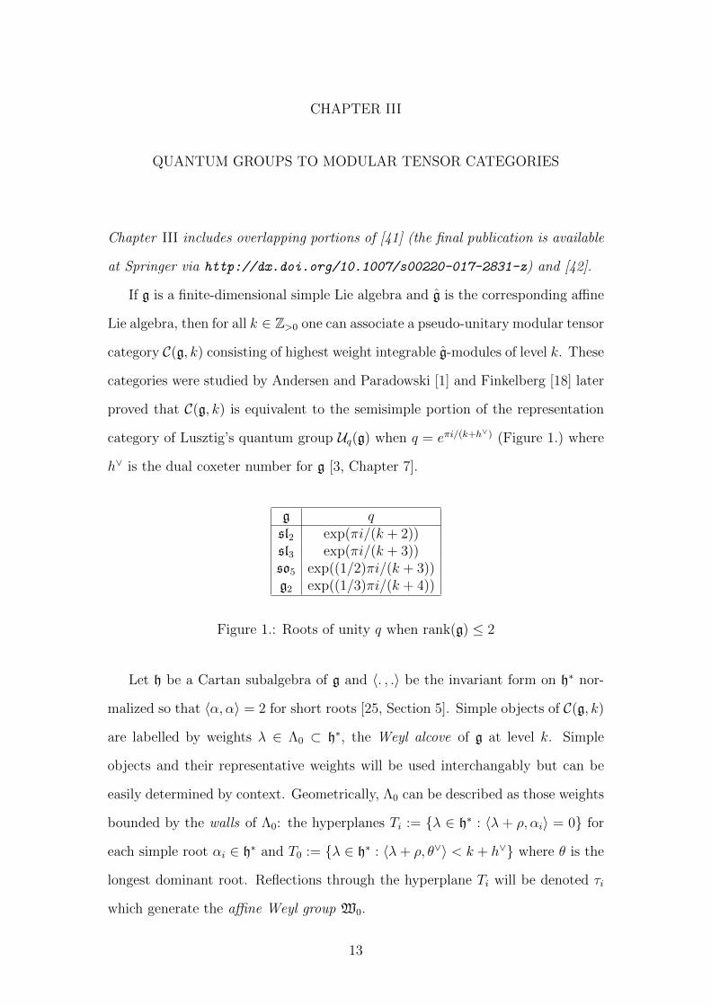
If g is a finite-dimensional simple Lie algebra and g is the corresponding affine

Lie algebra, then for all k ∈ Z>0 one can associate a pseudo-unitary modular tensor

category C(g, k) consisting of highest weight integrable g-modules of level k. These

categories were studied by Andersen and Paradowski [1] and Finkelberg [18] later

proved that C(g, k) is equivalent to the semisimple portion of the representation

category of Lusztig’s quantum group Uq(g) when q = eπi/(k+h∨) (Figure 1.) where

h∨ is the dual coxeter number for g [3, Chapter 7].

g qsl2 exp(πi/(k + 2))sl3 exp(πi/(k + 3))so5 exp((1/2)πi/(k + 3))g2 exp((1/3)πi/(k + 4))

Figure 1.: Roots of unity q when rank(g) ≤ 2

Let h be a Cartan subalgebra of g and 〈. , .〉 be the invariant form on h∗ nor-

malized so that 〈α, α〉 = 2 for short roots [25, Section 5]. Simple objects of C(g, k)

are labelled by weights λ ∈ Λ0 ⊂ h∗, the Weyl alcove of g at level k. Simple

objects and their representative weights will be used interchangably but can be

easily determined by context. Geometrically, Λ0 can be described as those weights

bounded by the walls of Λ0: the hyperplanes Ti := {λ ∈ h∗ : 〈λ + ρ, αi〉 = 0} for

each simple root αi ∈ h∗ and T0 := {λ ∈ h∗ : 〈λ+ ρ, θ∨〉 < k + h∨} where θ is the

longest dominant root. Reflections through the hyperplane Ti will be denoted τi

which generate the affine Weyl group W0.

13

If ρ is the half-sum of all positive roots of g then the dimension of the simple

object corresponding to the weight λ ∈ Λ0 is given by the quantum Weyl dimension

formula

dim(λ) =∏α�0

[〈α, λ+ ρ〉][〈α, ρ〉]

where [m] is the q-analog of m ∈ Z≥0 which for a generic parameter q is

[m] =qm − q−m

q − q−1= qm−1 + qm−3 + · · ·+ q−(m−3) + q−(m−1).

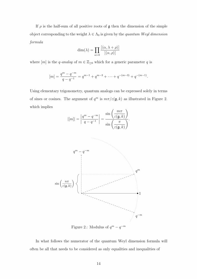
Using elementary trigonometry, quantum analogs can be expressed solely in terms

of sines or cosines. The argument of qm is mπ/ε(g, k) as illustrated in Figure 2.

which implies

|[m]| =∣∣∣∣qm − q−mq − q−1

∣∣∣∣ =

sin

(mπ

ε(g, k)

)sin

(π

ε(g, k)

) .

1

q−m

qm

qm − q−m

sin

(nπ

ε(g, k)

)

Figure 2.: Modulus of qm − q−m

In what follows the numerator of the quantum Weyl dimension formula will

often be all that needs to be considered as only equalities and inequalities of

14

dimensions with equal denominators appear. We will denote this numerator

dim′(λ). With the values of q found in Figure 1., dim(λ) ∈ R≥1 (and in par-

ticular [m] ∈ R>0 for all considered m ∈ Z>0) for all λ ∈ Λ0. The full twist on a

simple object λ ∈ Λ0 is given by θ(λ) = q〈λ,λ+2ρ〉 which is a root of unity depending

on g, k, and λ.

We refer the reader to [25, Sections 13,21–24] for concepts and results from

classical representation theory of Lie algebras.

3.1. Numerical Data and Fusion Rules for C(g, k) when rank(g) ≤ 2

Simple objects of C(sl2, k) are enumerated by s ∈ Z≥0 such that s ≤ k. Each

object, denoted by (s), corresponds to the weight sλ ∈ Λ0, where λ is the unique

fundamental weight. The dimension of (s) is given by dim(s) = [s + 1] and the

full twist on this object by

θ(s) = exp

(s(s+ 2)

4(k + 2)· 2πi

).

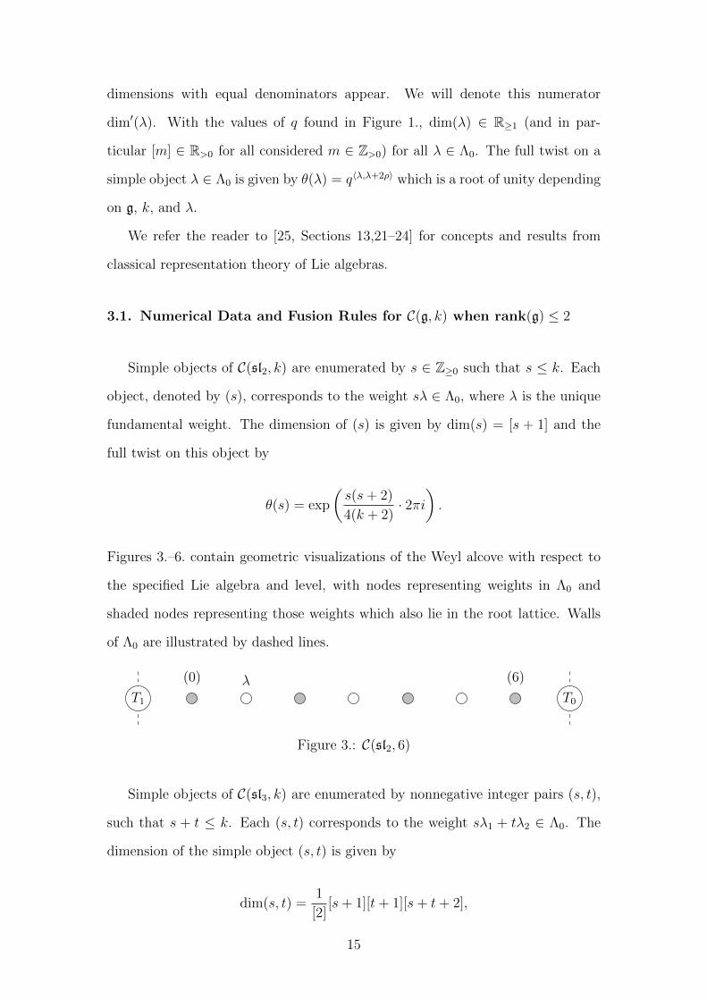
Figures 3.–6. contain geometric visualizations of the Weyl alcove with respect to

the specified Lie algebra and level, with nodes representing weights in Λ0 and

shaded nodes representing those weights which also lie in the root lattice. Walls

of Λ0 are illustrated by dashed lines.

(0) λ (6)

T0T1

Figure 3.: C(sl2, 6)

Simple objects of C(sl3, k) are enumerated by nonnegative integer pairs (s, t),

such that s + t ≤ k. Each (s, t) corresponds to the weight sλ1 + tλ2 ∈ Λ0. The

dimension of the simple object (s, t) is given by

dim(s, t) =1

[2][s+ 1][t+ 1][s+ t+ 2],

15

and using the trigonometric identities for quantum analogs, we have the following

proposition which will refer back to in future proofs.

Proposition 2. For all (s, t) ∈ Λ0

dim(s, t) =

sin

((s+ 1)π

k + 3

)sin

((t+ 1)π

k + 3

)sin

((s+ t+ 2)π

k + 3

)sin

(2π

k + 3

)sin2

(π

k + 3

) .

The twist on this object is given by

θ(s, t) = exp

(s2 + 3s+ st+ 3t+ t2

3(k + 3)· 2πi

).

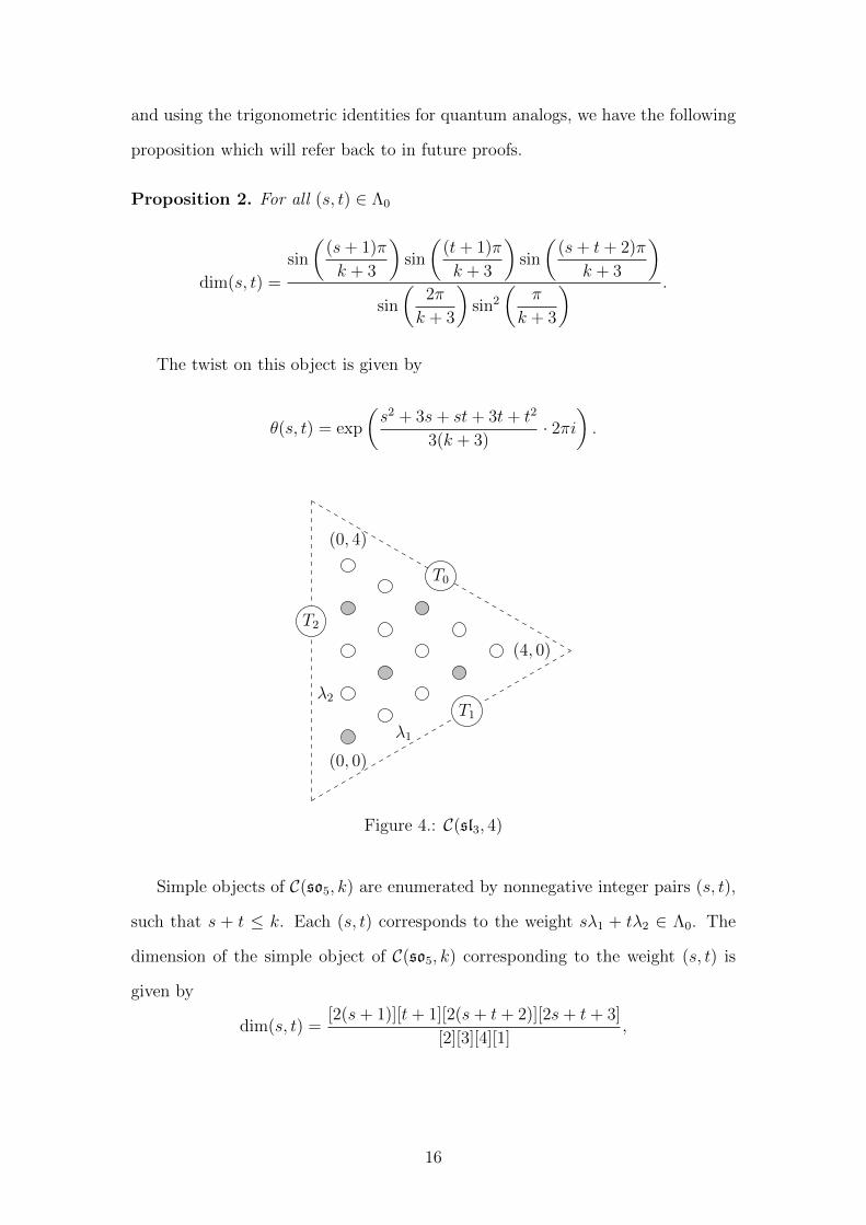
(0, 0)

λ2

(0, 4)

λ1

(4, 0)

T1

T2

T0

Figure 4.: C(sl3, 4)

Simple objects of C(so5, k) are enumerated by nonnegative integer pairs (s, t),

such that s + t ≤ k. Each (s, t) corresponds to the weight sλ1 + tλ2 ∈ Λ0. The

dimension of the simple object of C(so5, k) corresponding to the weight (s, t) is

given by

dim(s, t) =[2(s+ 1)][t+ 1][2(s+ t+ 2)][2s+ t+ 3]

[2][3][4][1],

16

and the twist on this object by

θ(s, t) = exp

(2s2 + 2st+ 6s+ t2 + 4t

4(k + 3)· 2πi

).

(0, 0)

λ1

(6, 0)

λ2

(0, 6)T1

T2

T0

Figure 5.: C(so5, 6)

Simple objects of C(g2, k) are enumerated by nonnegative integer pairs (s, t),

such that s + 2t ≤ k. Each (s, t) corresponds to the weight sλ1 + tλ2 ∈ Λ0. The

dimension of the simple object (s, t) is given by

dim(s, t) =[s+ 1][3(t+ 1)][3(s+ t+ 2)][3(s+ 2t+ 3)][s+ 3t+ 4][2s+ 3t+ 5]

[1][3][6][9][4][5],

17

and the twist on this object by

θ(s, t) = exp

(s2 + 3st+ 5s+ 3t2 + 9t

3(k + 4)· 2πi

).

(0,0)

λ2

λ1

(8,0)(0,4)

T2 T1

T0

Figure 6.: C(g2, 8)

Lastly we recall a result influenced by Andersen and Paradowski and proven

by Sawin as Corollary 8 in [39], giving a formula for the fusion rules in C(g, k).

18

Proposition 3 (Quantum Racah formula). If λ, γ, η ∈ Λ0 then

Nηλ,γ := dimC Hom(η, λ⊗ γ) is given by

Nηλ,γ =

∑τ∈W0

(−1)`(τ)mγ(τ(η)− λ),

where `(τ) is the length of a reduced expression of τ ∈ W0 in terms of τ1, τ2, τ3

and mλ(µ) is the dimension of the µ-weight space in the classical representation

of highest weight λ.

As in Lemma 1 of [38] this formula can be used to identify particular direct

summands of tensor products of simple objects in C(g, k). Based on slight nota-

tional discrepancies in the Quantum Racah formula in [38], we provide a proof

here based on that of Sawin’s.

Lemma 2 (Sawin). For any σ in the classical Weyl group W, and any γ, λ ∈ Λ0,

if λ+σ(γ) ∈ Λ0, then λ⊗γ contains λ+σ(γ) as a direct summand with multiplicity

one.

Proof. Assume that λ′ /∈ Λ0 is any weight conjugate to λ ∈ Λ0 under the action of

W0. Explicitly, there exists (τi1τi2 · · · τit) ∈ W0 (written as a reduced expression

in the generating simple reflections) such that

(τi1τi2 · · · τit)(λ′) = λ. (3)

Now let η ∈ Λ0 be arbitrary. The hyperplane of reflection corresponding to τit

lies between λ′ and η by assumption, so ‖τit(λ′)− η‖ < ‖λ′ − η‖. Repeating this

argument over all simple reflections in (3) shows that

‖λ− η‖ < ‖λ′ − η‖. (4)

With reference to the summands appearing in Proposition 3, assume that

19

mγ(τ(λ+ σ(γ))− λ) 6= 0 for some non-trivial τ ∈W0. Then

‖τ(λ+ σ(γ))− λ‖ ≤ ‖γ‖ (5)

because γ is heighest weight. Since λ + σ(γ) ∈ Λ0 and τ(λ + σ(γ)) is not, (4)

implies

‖γ‖ = ‖σ(γ)‖ = ‖(λ+ σ(γ))− λ‖ < ‖τ(λ+ σ(γ))− λ‖

contradicting the highest weight inequality in (5). Thus mγ(τ(λ + σ(γ)) − λ) is

possibly nonzero if and only if τ = id ∈W0 and thus

Nλ+σ(γ)λ,γ = (−1)0mγ((λ+ σ(γ))− λ) = mγ(σ(γ)) = 1.

It is necessary to the proof of future claims to consider the geometric inter-

pretation of the quantum Racah formula specifically for rank 2 Lie algebras [39,

Remark 4]. The notation and concepts introduced in this subsection will be used

prolifically throughout the proof of Theorem 5 and are illustrated by example in

Figure 7. to compute Nµλ,γ for arbitrary µ ∈ Λ0, λ := (3, 4), and γ := (3, 6) (white

node) in C(so5, 12).

Given λ, γ ∈ Λ0, the quantum Racah formula states that to calculate the

fusion coefficients Nµλ,γ for any µ ∈ Λ0 geometrically, one should compute Π(λ),

the classical weight diagram for the finite-dimensional irreducible representation

of highest weight λ, and (for visual ease) we illustrate its convex hull, Π(λ). For

this purpose reflections in the classical Weyl group are illustrated in Figure 7.a by

thin lines. One can then shift Π(λ) and Π(λ), so they are centered at γ, denoting

these shifted sets by Π(λ : γ) and Π(λ : γ). Now for a fixed weight µ ∈ Λ0, τ ∈W0

will contribute to the sum Nµλ,γ if and only if there exists µ′ ∈ Π(λ : γ) such that

τ(µ′) = µ. The walls of Λ0 are illustrated (and labelled) in Figure 7.b by dashed

lines and all contributing τ ∈W0 can be visualized by folding Π(λ : γ) along the

20

walls of Λ0 until it lies completely within Λ0. To emphasize effect of folding, the

folded portions of Π(λ : γ) are illustrated in Figure 7.b with emphasized shading,

while regions of Π(λ : γ) unaffected by folding are given a crosshatch pattern.

·················

·················

·················

·················

·················

·················

·················

·················

·················

·················

·················

·················

·················

·················

·················

·················

·················

·················

·················

·················

·················

·················

·················

·················

·················

·················

·················

·················

·················

·················

·················

·················

(a) Π(λ)

·················

·················

·················

·················

·················

·················

·················

·················

·················

·················

·················

·················

·················

·················

·················

·················

·················

·················

·················

·················

·················

·················

·················

·················

·················

·················

·················

·················

·················

·················

·················

·················

T1

T2

T0

(b) Π(λ : γ), folded

Figure 7.: λ⊗ γ ∈ C(so5, 12)

For arbitrary λ, γ, µ ∈ Λ0 there may be several τ ∈ W0 which contribute

(positively or negatively) to the sum Nµλ,γ in the quantum Racah formula, but

for many fusion coefficients the only contribution comes from the identity of W0

and are therefore easily determined to be zero or positive. In Figure 7.b, these

coefficients correspond to weights in Π(λ : γ) which also lie in the crosshatched

region.

Lemma 3. Fix λ, γ, µ ∈ Λ0. If

(1) µ ∈ Π(λ : γ), and

(2) τi(µ′) 6= µ for any µ′ ∈ Π(λ : γ) and i = 0, 1, 2,

then Nµλ,γ > 0.

Proof. By assumption (1), mλ(µ − γ) > 0 is one term in the quantum Racah

formula for Nµλ,γ. Any nontrivial τ contributing to Nµ

λ,γ, does so via µ′ ∈ Π(λ :

γ) conjugate to µ. But one can verify using elementary plane geometry that

21

τi(Π(λ : γ)

)⊂ Π(λ : γ) for each generating reflection i = 0, 1, 2. This observation

along with assumption (2) implies no reflections of length greater than or equal

to one may contribute to the desired fusion coefficient and moreover Nµλ,γ is equal

to mλ(µ− γ) > 0.

3.2. C(sl3, k)

Even though the duality in C(sl3, k) is clear for other reasons, its computation

is straightforward from Lemma 2.

Corollary 1. If (m1,m2) ∈ Λ0, then (m1,m2)∗ = (m2,m1).

Proof. Note that if C is a fusion category and X, Y ∈ C are simple, then by

adjointness of duality Y ∗ ' X if and only if

1 = dimk Hom(Y ∗, X) = dimk Hom(1, X ⊗ Y ).

Now if we denote the generating reflections σ1, σ2 ∈W, then

(σ2σ1σ2)(m2,m1) = −(m1,m2).

Thus (m1,m2) + (σ2σ1σ2)(m2,m1) = (0, 0) and by Lemma 2, (m1,m2)⊗ (m2,m1)

contains (0, 0) with multiplicity one.

We also collect a formula for the multiplicative central charge of C(g, k) [10,

Section 6.2] for future use.

Lemma 4. The multiplicative central charge of C := C(g, k) is given by

ξ(C) = exp

(2πi

8· k dim g

k + h∨

)

where dim g is the dimension of g as a C-vector space and h∨ is the dual Coxeter

number of g.

22

Note 4. Refer to the introduction in [39] for a complete list of dual Coxeter

numbers.

3.2.1. Fusion Subcategories of C(sl3, k). All fusion subcategories of C(g, k)

were classified by Sawin in Theorem 1 of [38]. For each level k ∈ Z>0, C(sl3, k)

has four fusion subcategories:

- the trivial fusion subcategory consisting of (0, 0);

- the entire category C(sl3, k);

- the subcategory consisting of weights (m1,m2) ∈ Λ0 also in the root lattice.

The collection of such weights will be denoted R0;

- the subcategory consisting of the weights (0, 0), (k, 0), and (0, k), hereby

called corner weights.

The proof of this classification relies on two facts that will be used in the sequel.

We provide proofs here based on the original arguments found in [38], specialized

to the case when g = sl3 for clarity and instructive purposes.

Lemma 5 (Sawin). If a fusion subcategory D ⊂ C(sl3, k) for k ≥ 2 contains weight

λ that is not a corner weight then λ⊗ λ∗ contains θ as a direct summand.

Proof. Note that θ is self-dual by Corollary 1, hence N θλ,λ∗ = Nλ

λ,θ and by Propo-

sition 3

Nλλ,θ =

∑τ∈W0

(−1)`(τ)mθ(τ(λ)− λ). (6)

If τ = id then the corresponding summand in (6) is mθ(0) = 2, the rank of sl3.

Now if the simple reflections τ1, τ2, τ3 are the generators of W0, the reasoning

leading to inequality (4) in the proof of Lemma 2 implies if i 6= j

‖(τiτj)(λ)− λ‖ > ‖τj(λ)− λ‖ > 0 (7)

for i, j = 1, 2, 3. If τj(λ) − λ contributes to the sum in (6), then τj(λ) − λ must

be a nonzero root. But inequality (7) implies that any τ ∈ W0 whose reduced

23

expression in terms of simple reflections has length greater than 1 causes τ(λ)−λ

to be longer than any root, and hence does not contribute to the sum in (6).

Moreover, the only negative contributions to (6) come from simple reflections.

If a weight µ ∈ Λ0 is adjacent to any generating hyperplane Ti for some i =

1, 2, 3 (see Figure 8.), then ‖τi(µ) − µ‖2 ≤ 2 otherwise ‖τi(µ) − µ‖2 > 2. Thus

τi(µ) − µ can contribute −1 to the sum in (6) if and only if µ is adjacent to

the hyperplane Ti. For µ ∈ Λ0 which are not corners, the number of adjacent

generating hyperplanes adjacent to µ is at most 1, proving Nλλ,θ > 0.

‖τ3(µ)− µ‖2 = 2

‖τ2(µ)− µ‖2 > 2•

•

•

•

•

•

•

•θ

•

•

•

•

•

•

•

•

•

•

•

•µ

•

α1

α2

T2

T3

Figure 8.: Adjacent vs. nonadjacent to Ti (level k = 5)

Lemma 6 (Sawin). If a fusion subcategory D ⊂ C(sl3, k) contains weight θ then

D contains the entire root lattice in the Weyl alcove, R0.

Proof. If λ ∈ R0 then there exists a path of length n ∈ Z≥0 of weights θ =

λ0, λ1, λ2, . . . , λn = λ in Λ0 such that λi+1 − λi is a root for 0 ≤ i ≤ n − 1. We

now proceed inductively on i to show each λi is in D. Assume λi is in D for some

0 ≤ i ≤ n − 1. The Weyl group W acts transitively on the roots, so there exists

σi ∈W such that σi(λ0) = λi+1 − λi. In other words λi + σi(λ0) = λi+1 ∈ Λ0 and

λ0 ⊗ λi contains λi+1 as a direct summand with multiplicity 1 by Lemma 2.

24

3.2.2. Prime Decomposition when 3 - k. In light of Proposition 1 the cate-

gories C(sl3, k) can be decomposed into a product of prime factors which we will

use in the sequel when 3 - k.

Proposition 4. The following are decompositions of C(sl3, k) into prime factors

when 3 - k:

(a) C(sl3, 1) ' C(Z/3Z, qω),

(b) C(sl3, 2) ' C(sl3, 2)′pt � C(sl3, 2)pt ' (C(sl2, 3)′pt)rev � C(Z/3Z, qω2),

and for all m ∈ Z>0

(c) C(sl3, 3m+ 1) ' C(sl3, 3m+ 1)′pt � C(sl3, 1), and

(d) C(sl3, 3m+ 2) ' C(sl3, 3m+ 2)′pt � C(sl3, 2)pt.

Note 5. Refer to Example 2 for the definitions of qω and qω2 .

Proof. We begin by computing the twists (Section 3.1.) of the corner weights:

θ(0, k) = θ(k, 0) = exp

(02 + 3(0) + (0)(k) + 3k + k2

3(k + 3)· 2πi

)= exp (2kπi/3) .

Thus if k ≡ 1 (mod 3) θ(0, k) = θ(k, 0) = ω and if k ≡ 2 (mod 3) then θ(0, k) =

θ(k, 0) = ω2.

The category C(sl3, 1) is pointed with three simple objects, and so it is deter-

mined by its twists found above. This identifies C(sl3, 1) ' C(Z/3Z, qω) which is

simple, proving (a).

For level k = 2 we first apply Muger’s decomposition (Section 2.1.) and no-

tice that C(sl3, 2)pt ' C(Z/3Z, qω2) based on the twist computations above. Its

centralizer has two simple objects and is not pointed. Thus C(sl3, 2)′pt is either

equivalent to C(sl2, 3)′pt or (C(sl2, 3)′pt)rev [10, Section 6.4][33]. Using the formula

found in Section 6.4 (2) of [10] we see

ξ(C(sl2, 3)′pt

)= exp

(2πi

8

(3 · 33 + 2

+ (−1)(3+1)/2

))= exp(7πi/10),

25

and thus by Lemma 1 (c),

ξ((C(sl2, 3)′pt)

rev)

= exp(13πi/10).

Using Lemma 1 (b) we have

ξ(C(sl3, 2)′pt

)=

ξ (C(sl3, 2))

ξ (C(sl3, 2)pt)=

exp(4πi/5)

exp(3πi/2)= exp(13πi/10),

proving (b) since both of these categories are known to be simple.

The decompositions in parts (c) and (d) follow directly from Muger’s decom-

position along with parts (a) and (b), and we are left with proving simplicity of the

centralizers of the pointed subcategories. For any k ∈ Z>0 the fusion subcategory

of corner weights ((0, 0), (k, 0), and (0, k)) is pointed. Proposition 3 gives

(0, k)⊗ (m1,m2) = (m2, k −m1 −m2) and

(k, 0)⊗ (m1,m2) = (k −m1 −m2,m1). (8)

Thus using the balancing equation [17, Proposition 8.13.8] we have

s(0,k),(m1,m2) = exp

(1

3(k − 2m1 −m2) · 2πi

)dim(m1,m2), and

s(k,0),(m1,m2) = exp

(1

3(k −m1 − 2m2) · 2πi

)dim(m1,m2).

This implies s(0,k),(m1,m2) = s(k,0),(m1,m2) = dim(m1,m2) if and only if m1 ≡ m2

(mod 3), that is to say (m1,m2) ∈ R0. And from [32, Proposition 2.5] sX,Y =

dim(X) dim(Y ) if and only if X and Y centralize one another . Moreover if

3 - k then the corners (0, k) and (k, 0) are not in the root lattice so by Sawin’s

classification of fusion subcategories (Section 3.2.1.), the centralizers of the pointed

subcategories are simple and thus prime.

We now take a moment to compute the central charge of C(sl3, k)′pt for future

26

use when k = 3m+1 or k = 3m+2 with m ∈ Z≥0 based on (c), (d) of Proposition

4 and the multiplicativity of ξ.

Corollary 2. For m ∈ Z≥0

(a) when k = 3m+ 1 (m 6= 0)

ξ(C(sl3, k)′pt

)= exp

(9m

6m+ 8πi

),

(b) and when k = 3m+ 2

ξ(C(sl3, k)′pt

)= exp

(3m− 7

6m+ 10πi

).

3.2.3. Simplicity of C(sl3, k)0A when 3 | k. When k = 3m for some m ∈ Z>0,

the object A = (0, 0) ⊕ (3m, 0) ⊕ (0, 3m) has the structure of a connected etale

algebra and we can consider the nondegenerate braided fusion category consisting

of dyslectic A-modules C0A := C(sl3, 3m)0A (Section 2.3.). The act of tensoring

with (3m, 0) or (0, 3m) geometrically results in a rotation of Λ0 by 120 degrees

counter-clockwise or clockwise, respectively, as illustrated in Figure 9..

.

. Stationary Objects

Free Objects⊗(6, 0)

⊗(6, 0)

⊗(6, 0)

Figure 9.: C0A at level k = 6 and the action of a corner weight

There are two types of simple objects in C0A:

27

- Free objects (Section 2.3.) are of the form F (λ) = λ ⊗ A for λ ∈ R0 not

equal to (m,m). These objects are the sum of the objects in orbits of size

three under the 120 degree rotations described above.

- Three stationary objects are isomorphic to (m,m) as objects of C(sl3, 3m),

but non-isomorphic as A-modules. If ρ1 : (m,m) ⊗ A −→ (m,m) is the

action on one of these A-modules then the others have actions given by

ρω = ωρ1 and ρω2 = ω2ρ1 where ω = exp(2πi/3).

Denote any of these three stationary objects as X ∈ C0A or collectively as

X1, X2, X3 ∈ C0A. At no point in what follows will it become important to dis-

tinguish their A-module structures and in fact doing so can lead to ambiguity in

computations as illustrated in the sl2 case described in Section 7 of [27].

Example 4. When k = 3 the only free object is the identity F (0, 0) and there

are three stationary objects X1, X2, X3 corresponding to the central weight (1, 1).

This category is pointed by Theorem 1.18 of [27] which states that for i = 1, 2, 3

dim(Xi) =dim(1, 1)

dim(A)=

sin2(π

3

)sin

(2π

3

)3 sin

(π3

)sin2

(π6

) = 1. (9)

The simple objects of C0A form an abelian group of order four, which is either cyclic

or the Klein-4 group. But the automorphism of this group given by tensoring

with (0, 3) or (3, 0) has order three so we must have C0A ' C(Z/2⊕ Z/2Z, q) with

quadratic form q : Z/2Z⊕ Z/2Z −→ C× which is 1 on the unit object and −1 on

the stationary objects. This category is evidently not simple as Z/2Z⊕Z/2Z has

many subgroups.

Example 5. We will also examine the case k = 6 as it is of great interest. There

are three stationary objects X1, X2, and X3, and three free objects Y1 = F (0, 0),

Y2 = F (1, 1), and Y3 = F (3, 3). The tensor structure of the free module functor

28

gives the fusion rules between the free objects:

Y2 ⊗A Y2 = Y1 ⊕ 2Y2 ⊕ 2Y3 ⊕X1 ⊕X2 ⊕X3,

Y2 ⊗A Y3 = 2Y2 ⊕ Y3 ⊕X1 ⊕X2 ⊕X3, and

Y3 ⊗A Y3 = Y1 ⊕ Y2 ⊕ Y3 ⊕X1 ⊕X2 ⊕X3.

For instance

Y2 ⊗A Y2 = F (1, 1)⊗A F (1, 1)

= F ((1, 1)⊗ (1, 1))

= F ((0, 0)⊕ (0, 3)⊕ (3, 0)⊕ (1, 1)⊕ (1, 1)⊕ (2, 2))

= Y1 ⊕ Y3 ⊕ Y3 ⊕ Y2 ⊕ Y2 ⊕ F (2, 2)

= Y1 ⊕ 2Y2 ⊕ 2Y3 ⊕X1 ⊕X2 ⊕X3.

Now to compute the remaining fusion rules note that at least one Xi is self dual,

hence all objects in the orbit of this Xi (under tensoring with a corner object)

must be self dual as well; i.e. all stationary objects Xi are self dual.

By comparing dimensions we must have that

Y2 ⊗A Xi = Y2 ⊕ Y3 ⊕Xj ⊕Xk, (10)

Y3 ⊗A Xi = Y2 ⊕ Y3 ⊕X`, (11)

and

Xr ⊗A Xs =

Y1 ⊕ Y3 ⊕Xt if r = s

Y2 ⊕Xu if r 6= s(12)

for some j, k, `, t, u = 1, 2, 3. We will now determine the unknown summands in

(10), (11), and (12). For instance the self duality of all objects implies if i 6= j, by

29

(12) we must have

1 = dimC Hom(Y2, Xi ⊗A Xj) = dimC Hom(Xi, Y2 ⊗A Xj).

Hence i, j, k are all distinct in (10). Similarly

0 = dimC Hom(Y3, Xi ⊗A Xj) = dimC Hom(Xi, Y3 ⊗A Xj),

which implies i = ` in (11) above. For any i, j = 1, 2, 3 denote the unknown

summand in Xi ⊗A Xj by Xi,j. We will show that if Xi 6= Xi,i then the following

equality cannot hold:

3 = dimC Hom(Xi ⊗A Xi, Xi ⊗A Xi) = dimC Hom(Y1, X⊗A4i ). (13)

To see the contradiction note that X⊗A3i,i = 2Y2 ⊕ Y3 ⊕ 2Xi ⊕ Xi,ii where Xi,ii is

the unknown summand in the product Xi ⊗A Xi,i. Our initial assumption and

the self duality of Xi guarantees Xi 6= X∗i,i and thus Xi 6= Xi,ii. But this would

imply dimC Hom(Xi ⊗A Xi, Xi ⊗A Xi) = 2 by the above computation of X⊗A3i ,

contradicting (13).

Now to determine the remaining fusion rule in (12), computing Y2⊗ (Xi⊗Xi)

and (Y2⊗Xi)⊗Xi using (10), (11), and the first part of (12) shows that Xi,i = Xi,

Xi,j and Xj,k are distinct. By symmetry of this computation Xj,i, Xj,j = Xj, and

Xj,k as well as Xk,i, Xk,j, and Xk,k = Xk are distinct triples as well. This proves

that Xi⊗Xj = Y2⊕Xk where i, j, k are distinct and the fusion rules are completely

determined.

Note 6. C(sl3, 6)0A is simple.

The S-matrix is now computed using the balancing equation [17, Proposition

8.13.8] which states that for all X, Y ∈ O(C) in a pre-modular category C,

sX,Y = θ(X)−1θ(Y )−1∑

Z∈O(C)

NZX,Y θ(Z) dim(Z).

30

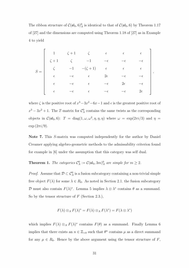
The ribbon structure of C(sl3, 6)0A is identical to that of C(sl3, 6) by Theorem 1.17

of [27] and the dimensions are computed using Theorem 1.18 of [27] as in Example

4 to yield

S =

1 ζ + 1 ζ ε ε ε

ζ + 1 ζ −1 −ε −ε −ε

ζ −1 −(ζ + 1) ε ε ε

ε −ε ε 2ε −ε −ε

ε −ε ε −ε 2ε −ε

ε −ε ε −ε −ε 2ε

,

where ζ is the positive root of x3−3x2−6x−1 and ε is the greatest positive root of

x3 − 3x2 + 1. The T -matrix for C0A contains the same twists as the corresponding

objects in C(sl3, 6): T = diag(1, ω, ω2, η, η, η) where ω = exp(2πi/3) and η =

exp (2πi/9).

Note 7. This S-matrix was computed independently for the author by Daniel

Creamer applying algebro-geometric methods to the admissability criterion found

for example in [6] under the assumption that this category was self dual.

Theorem 1. The categories C0A := C(sl3, 3m)0A are simple for m ≥ 2.

Proof. Assume that D ⊂ C0A is a fusion subcategory containing a non-trivial simple

free object F (λ) for some λ ∈ R0. As noted in Section 2.1. the fusion subcategory

D must also contain F (λ)∗. Lemma 5 implies λ ⊗ λ∗ contains θ as a summand.

So by the tensor structure of F (Section 2.3.),

F (λ)⊗A F (λ)∗ = F (λ)⊗A F (λ∗) = F (λ⊗ λ∗)

which implies F (λ) ⊗A F (λ)∗ contains F (θ) as a summand. Finally Lemma 6

implies that there exists an n ∈ Z>0 such that θn contains µ as a direct summand

for any µ ∈ R0. Hence by the above argument using the tensor structure of F ,

31

F (θ)n will contain F (µ) as a direct summand. In this case we have proven D = C0A

since all simple objects are direct summands of free objects (Section 2.3.).

The only case that remains is if the fusion subcategory D only contains sta-

tionary object(s) X ∈ C0A corresponding to the central weight (m,m) which we

will denote as ν for brevity.

Lemma 7. In C(sl3, 3m) with m ∈ Z>0, we have N νν,ν = m+ 1.

Proof. Proposition 3 gives

N νν,ν =

∑τ∈W0

(−1)τmν(τ(ν)− ν). (14)

For the simple reflections τ1, τ2, τ3 ∈W0, ‖τi(ν)− ν‖ > ‖ν‖ and by the reasoning

leading to inequality (4) in the proof of Lemma 2 the only nonzero term in (14)

comes from the identity in W0, i.e. Nνν,ν = mν(0). If p(µ) is the number of ways

of writing a weight µ as a sum of positive roots, by Kostant’s multiplicity formula

[25, Chapter 24.2]

mν(0) =∑σ∈W

(−1)`(σ)p(σ((m+ 1)α1 + (m+ 1)α2)− α1 − α2)

= p(mα1 +mα2)

because the argument of p is not dominant for any nontrivial elements of the

Weyl group. Now it suffices to note that because there are three positive roots,

α1, α2, α1 +α2, then p(mα1 +mα2) = m+ 1 because to count the number of ways

to write mα1 +mα2 as a sum of positive roots is the same as choosing how many

copies of α1 + α2 to use (the number of α1’s and α2’s are then determined).

To finish the proof of Theorem 1, we wish to show that some nontrivial simple

free object appears as a summand of X ⊗A X (1 is a summand of X ⊗A X∗ as

dimC Hom(1, X ⊗A X∗) = dimC Hom(X,X) = 1). We have already shown above

that this would imply the nontrivial simple free summand generates the entire

32

category C0A.

If X ⊗A X∗ does not contain a simple non-trivial summand different from X

then we must have

X ⊗A X∗ = 1⊕ nX

where n ∈ Z≥0 and n ≤ m+ 1 by Lemma 7. Using the additivity and multiplica-

tivity of dimension the above implies

dim(X)2 − n dim(X)− 1 = 0,

hence

dim(X) =n+√n2 + 4

2≤ m+ 3. (15)

By Proposition 2 and Theorem 1.18 of [27],

dim(X) =

sin2

((m+ 1)π

3(m+ 1)

)sin

((2(m+ 1)π

3(m+ 1)

)3 sin

(2π

3(m+ 1)

)sin2

(π

3(m+ 1)

)=

√3

8 sin

(2π

3(m+ 1)

)sin2

(π

3(m+ 1)

) .

But for m ≥ 2 the arguments of the above sines are are positive hence sin(x) < x

and we have

dim(X) >27√

3(m+ 1)3

16π3

which is strictly greater than m + 3 for m ≥ 3, contradicting the inequality in

(15). The case when m = 2 was described explicitly in Example 5.

33

CHAPTER IV

WITT GROUP RELATIONS

Chapter IV appeared in [41] (the final publication is available at Springer via

http://dx.doi.org/10.1007/s00220-017-2831-z).

4.1. Modular Invariants and Conformal Embeddings

Given a connected etale algebra A in a modular tensor category C one can

construct ZA ∈ Matn(Z≥0) where n = |O(C)|. The matrix ZA commutes with

the modular group action associated with the modular tensor category C, i.e. ZA

commutes with the S-matrix and T -matrix of C [27, Theorem 4.1]. Such matrices

have been referred to as (symmetric) modular invariants in the mathematical

physics literature [22, Definition 1].

Note 8. There is a slight discrepancy in vocabulary needed to use [27, Theorem

4.1] in the case of connected etale algebras in C(g, k). In particular this theorem

was proven assuming A is a “rigid C-algebra with θ(A) = idA”. The term C-

algebra in [27, Definition 1.1] corresponds to an associative, unital, commutative,

connected algebra in C. Thus connected etale algebras in C are also C-algebras.

The term rigid [27, Definition 1.11] requires a certain nondegenerate pairing A⊗

A → 1 which is guaranteed for connected etale algebras as noted in [10, Remark

3.4]. A proof of the fact that θ(A) = idA when A is a connected etale algebra in a

pseudo-unitary modular tensor category can be derived from paragraph 3 of [36,

Remark 2.19], or in Lemma 8.

To explicitly compute ZA from a connected etale algebra A ∈ C one should

decompose all dyslectic modules M ∈ C0A as objects of C: M =⊕

X∈O(C)NXMX,

with NXM ∈ Z≥0 and treating X as a formal symbol representing an object

34

X ∈ O(C), compute

∑M∈O(C0A)

|NXMX|2 =

∑X,Y ∈O(C)

ZX,YXY ,

for some ZX,Y ∈ Z≥0. The coefficient matrix ZA := ZX,Y is the modular invariant

associated to A.

Example 6. For a low-rank example consider C := C(sl2, 4) with five simple

objects: (0), (1), (2), (3), (4). The object A := (0) ⊕ (4) has the structure of a

connected etale algebra and C0A has three simple objects: (0)⊕ (4) and two objects

isomorphic to (2) with different A-module structures. We compute

∑M∈O(C0A)

|NXMX|2 = |(0) + (4)|2 + 2|(2)|2

= (0)(0) + (0)(4) + (4)(0) + (4)(4) + 2(2)(2),

which yields the following modular invariant. The reader may verify that ZA

commutes with the given S-matrix for C(sl2, 4).

ZA =

1 0 0 0 1

0 0 0 0 0

0 0 2 0 0

0 0 0 0 0

1 0 0 0 1

S =

1√

3 2√

3 1√

3√

3 0 −√

3 −√

3

2 0 −2 0 2√

3 −√

3 0√

3 −√

3

1 −√

3 2 −√

3 1

As the rank of g and the level k increase without bound across all C(g, k),

35

computing and classifying these modular invariants from a numerical standpoint

becomes an arduous task. A complete and rigorous classification only exists for

all levels k in the g = sl2 [7] and g = sl3 [22] cases, the latter being of particular

interest to our second main result. In particular there is an infinite family of such

modular invariants for sl3 occuring at levels k = 3m for some m ∈ Z≥1, arising

from the connected etale algebras described in Section 3.2.3. (there is also a trivial

modular invariant corresponding to the unit object considered as a connected etale

algebra). All other symmetric modular invariants will be labelled exceptional. The

following is a consequence of the classification of sl3 modular invariants due to

Gannon [22, Theorem 1].

Theorem 2 (Gannon). The only exceptional symmetric modular invariants for

sl3 occur at levels k = 5, 9, and 21.

Translating this into our discussion of Witt class representatives and the de-

compositions/reductions found in Sections 3.2.2. and 3.2.3., we have the following

corollary.

Corollary 3. The categories C(sl3, 3m + 1)′pt and C(sl3, 3m + 2)′pt are completely

anisotropic for m ∈ Z>0 and 3m+ 2 6= 5, while C(sl3, 3m)0A is completely

anisotropic for m ∈ Z≥2 and 3m 6= 9, 21.

Proof. We begin by noting that A ∈ C(sl3, 3m) as described in Section 3.2.3. must

be a maximal connected etale algebra when k 6= 9, 21. If not, by the method de-

scribed in the introduction to this section, one could create an exceptional modular

invariant at this level contradicting Theorem 2. Hence C(sl3, 3m)0A is completely

anisotropic when k 6= 9, 21.

By this exact argument, no nontrivial connected etale algebra exists in

C(sl3, 3m+ 1) or C(sl3, 3m+ 2) when 3m+ 2 6= 5. Finally if A is a connected etale

algebra in a braided fusion category C, and D is any other braided fusion category,

then A� 1 is a connected etale algebra in C � D [11, Section 3.2]. Moreover the

lack of connected etale algebras in C(sl3, 3m+1) or C(sl3, 3m+2) when 3m+2 6= 5

36

implies that the simple factors of these categories are completely anisotropic as

well.

In the cases k = 5, 9, 21 we will use alternative methods to identify completely

anisotropic representatives of the Witt classes of C(sl3, k). In particular the the-

ory of conformal embeddings can be used to construct relations among the classes

[C(g, k)] for any finite dimensional simple Lie algebra g [10, Section 6.2]. A com-

plete classification of such conformal embeddings is given in [2] and [40].

Each conformal embedding g ⊂ g′ gives rise to equivalences of the form

[C(g, k)] = [C(g′, k′)] for some levels k, k′ ∈ Z>0. Three conformal embeddings

are of interest for the classification of sl3 relations: A2,9 ⊆ E6,1, A2,21 ⊆ E7,1, and

A2,5 ⊆ A5,1. These embeddings will be used implicitly in the proof of the following

proposition.

Proposition 5. The following relations hold in the Witt group W:

(a) [C(sl3, 9)] = [C(sl3, 2)pt]

(b) [C(sl3, 21)] = [(C(sl2, 1)rev], and

(c) [C(sl3, 5)] = [C(sl5, 1)] = [C(Z/5Z, q)].

Proof. The category C(E6, 1) is pointed with three simple objects. Using Propo-

sition 4 we compute ξ(C(E6, 1)) = exp((2πi)/8(1 · 78)/(1 + 12)) = −i. Pointed

categories C(Z/3Z, q) are determined by their central charge and thus C(E6, 1) '

C(Z/3Z, qω2) ' C(sl3, 2)pt, which is simple and completely anisotropic implying re-

lation (a). Similarly the category C(E7, 1) is pointed with two simple objects. Us-

ing Proposition 4 we find ξ(C(E7, 1)) = exp((2πi/8)(1·133)/(1+18)) = (1−i)/√

2.

Pointed categories C(Z/2Z, q) are also determined by their central charge and

thus C(E7, 1) ' C(Z/2Z, q−), where q−(1) = −i, which is simple and completely

anisotropic. This is a familiar category coming from sl2. Proposition 4 implies

ξ(C(sl2, 1)) = exp((2πi/8)(1 · 3)/(1 + 2)) = (1 + i)/√

2. Lemma 1 (c) then implies

ξ(C(sl2, 1)rev) = (1 − i)/√

2 which gives relation (b). Lastly C(sl5, 1) is pointed

37

with five simple objects. As noted in Example 6.2 of [10], C(sln, 1) ' C(Z/nZ, q)

where q(`) = exp (πi`2(n− 1)/n)) and hence relation (c) follows.

4.2. A Classification of sl3 Relations

Theorem 3. The only relations in the Witt group of nondegenerate braided fusion

categories W coming from the subgroup generated by [C(sl3, k)] are the following:

(3.a) [C(sl3, 1)]4 = [Vec],

(3.b) [C(sl3, 3)]2 = [Vec],

(3.c) [C(sl3, 5)]2 = [Vec],

(3.d) [C(sl3, 1)]3 = [C(sl3, 9)], and

(3.e) [C(sl3, 21)]8 = [Vec].

Proof. Our approach to this proof will be to show that the above relations hold,

and then prove that these are the only relations which can exist by identifying the

unique representatives of each class [C(sl3, k)] as described in Section 2.4..

Since C(sl3, k) in equations (3.a)–(3.e) above are all Witt equivalent to a

pointed modular tensor category by the computations in Proposition 4 (a), Exam-

ple 4, and Proposition 5, the relations follow from the exposition in Appendix A.7

of [14] which explicitly describes the pointed subgroup Wpt ⊂ W . The remaining

question is whether these relations are exhaustive.

By Proposition 4, Theorem 1, and Corollary 3 for m ∈ Z≥0 we have collected

simple, completely anisotropic, nondegenerate braided fusion categories

C(sl3, 3m+ 1)′pt, for m 6= 0 (16)

C(sl3, 3m+ 2)′pt, for m 6= 1 (17)

C(sl3, 3m)0A, for m 6= 0, 1, 3, 7 (18)

We claim the categories in the above families are not equivalent and will prove

38

this by noting their central charges are distinct using Lemma 4 and Lemma 2. For

m = 0, 1, 2 one can manually verify the proposed central charges are distinct. If

arg(z) is the complex argument of z ∈ C, for m ∈ Z≥3 we have

0 < arg ξ(C(sl3, 3m+ 2)′pt) < π/2 (19)

π < arg ξ(C(sl3, 3m+ 1)′pt) < 3π/2, and (20)

3π/2 ≤ arg ξ(C(sl3, 3m)0A) < 2π. (21)

Recall the Witt group of slightly degenerate braided fusion categories, sW , in-

troduced in [11]. Studying this alternate Witt group is advantageous because

slightly degenerate braided fusion categories admit a unique decomposition into

s-simple components [11, Definition 4.9, Theorem 4.13], and consequentially there

are no nontrivial relations in sW other than relations of the form [C] = [C]−1

[11, Remark 5.11]. The categories in (16)–(18) are simple and unpointed, hence

their image under the group homomorphism S :W −→ sW [11, Section 5.3] is s-

simple. Their image is also completely anisotropic and slightly degenerate. Hence

any nontrivial relation in W between these categories would pass to a relation in

sW under the map S and this relation is nontrivial provided they are not in the

kernel of S, which is WIsing consisting of the Witt equivalence classes of the Ising

braided categories.

When [C] = [C]−1 in sW , C ' Crev which implies ξ(C) = ±1. This cannot be

true of the categories in (16)–(18) by the inequalities in (19)–(21) and a manual

check in the case m = 0, 1, 2. Thus the relations (3.a)–(3.e) are exhaustive.

Once relations in the subgroups individually generated by [C(sl2, k)] and

[C(sl3, k)] are classified one should then classify all relations between the two fam-

ilies.

39

Theorem 4. All nontrivial relations between the equivalency classes [C(sl2, k)]

and [C(sl3, k)] are generated by

(4.a) [C(sl3, 3)] = [C(sl2, 2)]8,

(4.b) [C(sl3, 3)][C(sl2, 2)]11 = [C(sl2, 6)]2,

(4.c) [C(sl3, 3)][C(sl2, 2)]15 = [C(sl2, 10)]7,

(4.d) [C(sl3, 21)][C(sl2, 1)] = [Vec],

(4.e) [C(sl3, 2)][C(sl2, 28)] = [C(sl3, 9)],

(4.f) [C(sl2, 4)] = [C(sl3, 1)],

(4.g) [C(sl2, 4)]3 = [C(sl3, 9)],

(4.h) [C(sl3, 6)][C(sl2, 16)] = [Vec], and

(4.i) [C(sl3, 4)][C(sl3, 1)] = [C(sl2, 12)].

To organize the search for these relations we will proceed in two stages: first

we consider coincidences between the sl3 relations from Theorem 3 and those sl2

relations found in [11, Section 5.5]:

[C(sl2, 1)]8 = [Vec], (22)

[C(sl2, 8)] = [C(sl2, 3)]−2[C(sl2, 1)]2, (23)

[C(sl2, 28)] = [C(sl2, 3)][C(sl2, 1)]−1, (24)

[C(sl2, 4)]4 = [Vec], (25)

[C(sl2, 2)]16 = [Vec], (26)

[C(sl2, 10)] = [C(sl2, 7)]7, and (27)

[C(sl2, 6)]2 = [C(sl2, 2)]3. (28)

Secondly we compare the lists of simple completely anisotropic Witt class

40

representatives for sl3 found in (16)–(18) and those for sl2 found in [11, Section

5.5]:

C(sl2, 2`+ 1)′pt, ` ≥ 1, (29)

C(sl2, 4`)0A, ` ≥ 3, ` 6= 7, and (30)

C(sl2, 4`+ 2)′pt, ` ≥ 3. (31)

For the first stage we have [C(sl3, 3)] = [C(sl3, 3)0A] is in WIsing. By (26) this is

a cyclic group of order 16 which is generated by [C(sl2, 2)], giving relation (4.a).

Multiplying relation (4.a) by [C(sl2, 2)]11 gives relation (4.b) using (28) and mul-

tiplying relation (4.a) by [C(sl2, 2)]15 gives relation (4.c) using (27).

Proposition 5 (b) implies relation (4.d). The relation implied by Proposition 4

(b) is [C(sl3, 2)][C(sl2, 3)′pt] = [C(sl3, 2)pt]. But together with (24) and Proposition

5 (a) we have relation (4.e).

Relation (25) is very similar to relations (3.a) and (3.c), and this is no coinci-

dence since there exists a conformal embedding A1,4 ⊂ A3,1, yielding relation (4.f).

Lastly cubing relation (4.f) and applying relation (3.d) implies relation (4.g).

For stage 2 of our proof, a first deduction can be made by noting that the cate-

gories (29) and (31) are self dual. There are only three self dual categories in (16)–

(18): C(sl3, 2)′pt, C(sl3, 3)0A, and C(sl3, 6)0A. The first is equivalent to (C(sl2, 3)′pt)rev

as noted in Proposition 3.2.2. (b) and the implied relations were discussed above,

while the Witt equivalence class of the second was previously treated as an ele-

ment of WIsing. It remains to show that C(sl3, 6)0A is not equivalent to C(sl2, 11)′pt

since these categories have the same number of simple objects. To this end the

formula in [10, Section 6.4 (1)] and Lemma 4 imply their central charges are not

equal.

The last step of stage 2 is to check that none of the categories C(sl2, 4`)0A are

equivalent to the categories in (16)–(18) (or their reverse categories). We will do

41

so by comparing central charges. Lemma 4 states for ` ∈ Z≥1

arg ξ(C(sl2, 4`)0A

)=

3`π

4`+ 2

and thus π/2 < arg ξ (C(sl2, 4`)0A) < π. There are possible exceptional equiv-

alences of the form C ' Drev since arg ξ (C(sl2, 4)0A) + arg ξ (C(sl3, 9)0A) = 2π,

arg ξ (C(sl2, 16)0A) + arg ξ (C(sl3, 6)0A) = 2π, arg ξ (C(sl2, 28)0A) + arg ξ(C(sl3, 2)′pt) =

0, and arg ξ (C(sl2, 12)0A) = arg ξ(C(sl3, 4)′pt). The first case was considered in

relation (4.g). In the second case not much work is needed since there is a con-

formal embedding A2,6 × A1,16 ⊂ E8,1 which gives relation (4.h). The third case

was considered in relation (4.e). The last case is caused from the equivalence

C(sl3, 4)′pt ' C(sl2, 12)0A by the classification of rank 5 modular tensor categories

[6], giving relation (4.i).

42

CHAPTER V

CONNECTED ETALE ALGEBRAS IN C(g, k)

Chapter V has previously appeared in [42].

The results of Chapter IV relied heavily on Theorem 2. There is no known proof

of an analgous statement for Lie algebras other than sl2 and sl3. In Theorem 5 we

provide a bound on levels k for which exceptional symmetric modular invariants

can exist in C(so5, k) and C(g2, k), reproving this known result for C(sl2, k) and

C(sl3, k) to demonstrate the generality of the argument.

5.1. Technical Machinery

The numerical conditions for an algebra in a pseudo-unitary pre-modular cat-

egory to be connected etale are quite restrictive. In particular the full twist on

such an algebra is trivial as we will prove below. This result is due to Victor

Ostrik, although a proof does not appear in the literature to our knowledge. The

full twist need not be trivial if the assumption of pseudo-unitary is removed as the

following example illustrates.

Example 7. The fusion category of complex Z/2Z-graded vector spaces has two

possible (symmetric) pre-modular structures, distinguished by the full twist on

the non-trivial simple object θ(X) = ±1. The trivial twist corresponds to the

pseudo-unitary category Rep(Z/2Z), while the nontrivial twist corresponds to

sVec, the category of complex super vector spaces [17, Example 8.2.2]. The object

A := 1⊕X has a unique structure of a connected etale algebra in both cases, but

θ(A) 6= idA in sVec, which is not pseudo-unitary (i.e. dim(X) = −1).

Lemma 8. If C is a pseudo-unitary premodular category and A is a connected

etale algebra in C, then θ(A) = idA.

43

Proof. The composition ϕ : A ⊗ Am→ A

εA→ 1 is non-degenerate [10, Remark

3.4], where εA arises from A being connected (and is unique up to scalar mul-

tiple). Note that the commutativity of A implies ϕsX∗,XsX,X∗ = ϕ. We can

then rewrite sX∗,XsX,X∗ using the balancing axiom [3, Equation 2.2.8] to yield

θ(X)θ(X∗)θ(1)−1 = 1 because ϕ is nondegenerate. Moreover θ(X) = ±1. So we

may now decompose A = A+ ⊕ A− where A± is the sum of simple summands of

A with twist ±1, respectively. We will deduce that A− is empty in the remainder

of the proof.

The commutativity of A = A+ ⊕ A− implies this decomposition is a Z/2Z-

grading again by the balancing axiom, i.e. θ(X ⊗ Y ) = θ(X)θ(Y ) for all simple

X, Y ⊂ A. Thus m restricts to a multiplication morphism A+ ⊗ A+ → A+. We

now aim to prove that A+ is a connected etale algebra. The commutativity of

A+ is clear from the commutativity of A and θ(1) = 1 by the balancing axiom

[3, Equation 2.2.9] so A+ is connected. It remains to show that A+ is separable,

i.e. CA+ is semisimple. This follows from [27, Theorem 3.3] by recalling that A+

is rigid (in the sense of Kirillov and Ostrik) because A+ ⊗ A+ m→ A+ εA→ 1 is

non-degenerate, and dim(A) 6= 0 since C is pseudo-unitary.

In the language of [10, Section 3.6], A with the inclusion A+ → A is known as

a commutative algebra over A+ and thus A can be considered as a commutative

algebra in D := C0A+ . Proposition 3.16 of [10] then implies A (as an algebra in D)

is connected etale as well. We also note that θ(A+) = idA+ along with Theorem

1.18 of [27], implies dim(D) =∑

X∈O(D) dimD(X)2 is equal to

∑X∈O(D)

(dimC(X)

dimC(A)

)2

= FPdimC(A)−2∑

X∈O(D)

FPdimC(X)2 (32)

= FPdimC(A)−2FPdim(C)

= FPdim(D). (33)

where (32) follows from C being pseudo-unitary and [10, Corollary 3.32] implies

(33). Moreover we have shown D is pseudo-unitary by Proposition 8.23 of [16].

44

Now assume X ⊂ A is a simple summand of A (as an object of D) which is

distinct from A+ = 1D. An immediate consequence is that X ⊂ A−, should such

an object exist. But X ⊗D X is a quotient of X ⊗X [27, Theorem 1.5] which, by

the Z/2Z-grading of A, implies X ⊗D X ⊂ A+ = 1D. The simplicity of the unit

object 1D = A+ then implies X ⊗D X = 1D.

Lastly we consider the fusion subcategory E ⊂ D generated by X, which by

the above reasoning is equivalent to the category of Z/2Z-graded vector spaces

(as a fusion category). The spherical structure of E which is inherited from D,

must be the nontrivial one since θ(X) = −1 (see Example 7) and thus E = s Vec,

a contradiction to D being pseudo-unitary. Moreover no such X can exist and

A = A+.

Now let A be a connected etale algebra in C := C(g, k) where g is sl3, so5, or g2

and (`,m) ⊂ A be a nontrivial summand of A which is minimal in the sense that

`+m is minimal in the case of sl3 and so5, and `+ (3/2)m is minimal in the case

of g2. The reasons for this distinction will be explained in the proof of Lemma 9.

Note 9. Our goal is not to reprove Theorem 5 in the rank 1 case so it will be

satisfactory to point out the following lemmas can be restated for C(sl2, k) where

(`) is the analogous minimal nontrivial summand of A ∈ C(sl2, k).

Lemma 9. If (s, t) ∈ Λ0 and 2(s + t) < ` + m in the case g = sl3, so5, or

2(s + (3/2)t) < ` + (3/2)m in the case g = g2, then (s, t) ⊗ A is a simple right

A-module.

Proof. Label λ := (s, t). Then we have by [35, Lemma 2, Lemma 4]

HomCA(λ⊗ A, λ⊗ A) = HomC(λ, λ⊗ A) = HomC(λ⊗ λ∗, A). (34)

The highest weight in Π(λ : λ∗) is γ := (s + t, s + t) when g = sl3 and γ :=

(2s, 2t) when g = so5, g2. The respective assumptions on (s, t) relative to (`,m)

in our hypotheses imply γ 6= (`,m) and it remains to check no other weights

45

(s′, t′) ∈ Π(λ : λ∗) are equal to (`,m) either. To this end it will suffice to check

γ − α 6= (`,m) for each simple root α since our claim follows inductively on

dominance ordering. If g = sl3, γ − α1 = (s + t− 2, s + t + 1) which is not equal

to (`,m) since s + t − 2 + s + t + 1 = 2(s + t) − 1 < ` + m and symmetrically

for α2. If g = so5, γ − α1 = (2s − 2, 2t + 2) which is not equal to (`,m) since

2s − 2 + 2t + 2 = 2(s + t) < ` + m and γ − α2 = (2s + 1, 2t − 2) which is not

equal to (`,m) since 2s + 1 + 2t − 2 = 2(s + 2) − 1 < ` + m. Lastly if g = g2,

γ−α1 = (2s− 2, 2t+ 1) which is not equal to (`,m) since 2s− 2 + (3/2)(2t+ 1) =

2(s+ (3/2)t)− 1/2 < `+ (3/2)m, and γ −α2 = (2s+ 3, 2t− 2) which is not equal

to (`,m) since 2s+ 3 + (3/2)(2t− 2) = 2(s+ (3/2)t) < `+ (3/2)m. Moreover the

right-hand side of (34) is one-dimensional and λ⊗A is a simple object in CA.

Lemma 10. If M ∈ CA, and (s, t) ⊂M satisfies the hypotheses of Lemma 9, then

(s, t)⊗ A is a right A-submodule of M .

Proof. As in the proof of Lemma 9 with λ := (s, t), compute HomCA(λ⊗A,M) =

HomC(λ,M). By assumption and Lemma 9, λ ⊗ A is simple, hence the result is

proven since the right-hand side is nontrivial.

Corollary 4. For all (s, t) ∈ Λ0 and {(si, ti)}i∈I , collections of simple summands

of M = (s, t)⊗ A satisying the assumptions of Lemma 9,

∑i∈I

dim′(si, ti) ≤ dim′(s, t).

Proof. Apply Lemma 10 to each element of {(si, ti)}i∈I . For each (si, ti) we then

have (si, ti)⊗ A ⊂ (s, t)⊗ A. Taking dimensions of the containment provides the

inequality, then dim(A) can be divided out and denominators cleared.

Exact computations are often intractable with quantum analogs so we now

collect a set of results that will be used frequently in the sequel to verify when

inequalities of the type in Corollary 4 are true or false. An illustration of the

trigonometric formulas for qn ± q−n in terms of sine or cosine when q is a root of

46

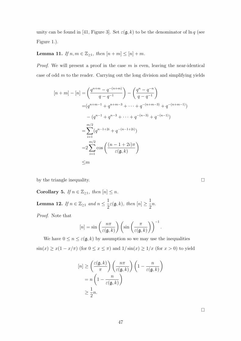
unity can be found in [41, Figure 3]. Set ε(g, k) to be the denominator of ln q (see

Figure 1.).

Lemma 11. If n,m ∈ Z≥1, then [n+m] ≤ [n] +m.

Proof. We will present a proof in the case m is even, leaving the near-identical

case of odd m to the reader. Carrying out the long division and simplifying yields

[n+m]− [n] =

(qn+m − q−(n+m)

q − q−1

)−(qn − q−n

q − q−1

)=(qn+m−1 + qn+m−3 + · · ·+ q−(n+m−3) + q−(n+m−1))

− (qn−1 + qn−3 + · · ·+ q−(n−3) + q−(n−1))

=

m/2∑i=1

(qn−1+2i + q−(n−1+2i))

=2

m/2∑i=1

cos

((n− 1 + 2i)π

ε(g, k)

)≤m

by the triangle inequality.

Corollary 5. If n ∈ Z≥1, then [n] ≤ n.

Lemma 12. If n ∈ Z≥1 and n ≤ 1

2ε(g, k), then [n] ≥ 1

2n.

Proof. Note that

[n] = sin

(nπ

ε(g, k)

)(sin

(π

ε(g, k)

))−1.

We have 0 ≤ n ≤ ε(g, k) by assumption so we may use the inequalities

sin(x) ≥ x(1− x/π) (for 0 ≤ x ≤ π) and 1/ sin(x) ≥ 1/x (for x > 0) to yield

[n] ≥(ε(g, k)

π

)(nπ

ε(g, k)

)(1− n

ε(g, k)

)= n

(1− n

ε(g, k)

)≥ 1

2n.

47

5.2. Exceptional Algebras

In [27], connected etale algebras in C(sl2, k) are organized into an ADE clas-

sification scheme paralleling the classification of simply-laced Dynkin diagrams.

The connected etale algebra of type A is the trivial one given by the unit object

1 ∈ C(sl2, k). Those connected etale algebras of type D arise at even levels in

the following manner. The fusion subcategory C(sl2, 2k)pt ⊂ C(sl2, 2k) generated

by invertible objects is equivalent to Rep(Z/2Z) and all connected etale algebras

in Rep(Z/2Z) are in one-to-one correspondence with subgroups of Z/2Z as the

additional cohomological data from [34, Theorem 3.1] is trivial for cyclic groups.

Type A algebras correspond to the trivial subgroup in the type D construction,

so we will refer to both types as standard in this exposition, and any algebra that

does not arise from this construction as exceptional.

Example 8. Extending the notation from Section 3.1., simple objects of C(sln, nk)

for k ∈ Z≥1 are enumerated by positive integer (n−1)-tuples (s1, s2, . . . , sn−1) such

that s1 + s2 + · · ·+ sn−1 ≤ nk. The fusion subcategory C(sln, nk)pt ' Rep(Z/nZ)

has simple objects (s1, s2, . . . , sn−1) such that si = nk and sj = 0 for all j 6= i,

along with the trivial object. Standard connected etale algebras in C(sln, nk)

are again in one-to-one correspondence with subgroups of Z/nZ. All exceptional

connected etale algebras in C(sl2, k) are succinctly listed in [27, Table 1], while all

exceptional connected etale algebras in C(sl3, k) are listed using modular invariants

[22, Equations 2.7d,2.7e,2.7g] at levels k = 5, 9, 21. The theory of conformal

embeddings provides examples of exceptional connected etale algebras in C(sl4, k)

at levels k = 4, 6, 8, which are described in detail in [9].

Example 9. There are no nontrivial standard connected etale algebras in C(g2, k)

since C(g2, k)pt ' Vec, but there are two standard connected etale algebras in

C(so5, 2k) since C(so5, 2k)pt ' Rep(Z/2Z) corresponding to (0, 0) and (0, 0) ⊕

(k, 0). For odd levels k, θ(k, 0) = −1 and so by Lemma 8, (0, 0)⊕ (k, 0) does not

have the structure of a connected etale algebra. As in Example 8, the theory of

48

conformal embeddings provides examples of exceptional connected etale algebras

in C(g2, k) at levels k = 3, 4 and C(so5, k) at levels k = 2, 3, 7, 12, which are

described in detail in [8].

Theorem 5. There exist finitely many levels k ∈ Z≥1 such that C(so5, k) or

C(g2, k) contains an exceptional connected etale algebra.

The proof of this result is contained in Section 5.3. but illustrated below in the

following example for sl2 and sl3.

Example 10 (C(sl2, k)). If A is an exceptional connected etale algebra in C(sl2, k)

with minimal nontrivial summand (`), Lemma 8 applied to the full twist formula

in Section 3.1. implies (`) is in the root lattice, i.e. ` is even, say ` = 2m for

some m ∈ Z≥1 and 2m < k. Explicit fusion rules for C(sl2, k) are well-known [10,

Section 2.8], and we see that (m + 3) ⊗ (2m) contains summands (m − 1) and

(m− 3) provided 3 ≤ m < k. Moreover Corollary 4 then implies

[m] + [m− 2] < [m+ 4] (35)

< [m] + 4 (36)

⇒ 1

2(m− 2) < 4 (37)

where (36) results from applying Corollary 5 to the right-hand side of (35) and

(37) results from applying Lemma 12 to the left-hand side of (36) which is justified

because 2m < k implies m− 2 ≤ (1/2)(k + 2). The inequality in (37) is false for

m > 9. Moreover θ(`) = 1 by Lemma 8 and so m(m + 1) − 2 ≥ k which implies

k ≤ 88 if m ≤ 9.

Note 10. It is possible to show from the definition of [n] that the inequality in

(35) is false in a more restricted setting: m > 5, which then implies k ≤ 28. But

there exists an exceptional connected etale algebra in C(sl2, 28) corresponding to

the object (0)⊕ (10)⊕ (18)⊕ (28) (type E8 in the ADE classification [27, Section

6]) and so this bound is tight. Even for Lie algebras of rank 2, computing precisely

49

when such an inequality is true becomes unrealistically complex. For the purposes

of Theorem 5 any bound will suffice.

Now let A be an exceptional connected etale algebra in C(sl3, k) with minimal

nontrivial summand (`,m) (i.e. `+m is minimal). Using duality ((`,m)∗ = (m, `))

and rotation of Λ0 by 120 degrees (tensoring with (0, k)), every (`,m) ∈ Λ0 is

conjugate to one (`′,m′) such that m′ ≤ `′ ≤ k/2. In what follows, the summands

of (`,m)∗ ⊗ (`,m) will be computed and these summands are invariant under

duality and rotation. We will show `′ + m′ is bounded for such a conjugate. To

do so we claim if m ≤ ` ≤ k/2, then

bx/2c⊕i=0

(i, i) ⊂ (m, `)⊗ (`,m). (38)

The set Π(m, ` : `,m) illustrated in Figure 10. (refer to Section 3.1. for descriptions

of the notation and visualization used) is a hexagon (triangle in the degenerate

case m = 0) with vertex (0, 0) and circumcenter (`,m). In particular (i, i) ∈

Π(m, ` : `,m) for 0 ≤ i ≤ bx/2c (black nodes in Figure 10.). The angles formed

between Π(m, ` : `,m) and T1, T2 are 30 degrees when they exist. Therefore, when

folded over T1, T2, the edges of Π(m, ` : `,m) containing (0, 0) are parallel to the

line formed by the weights 0 ≤ i ≤ bx/2c, implying τj(µ) 6= (i, i) for any i ≥ 0 and

j = 1, 2. Furthermore m ≤ ` ≤ k/2 ensures there is no contribution from τ0 to

N(i,i)(m,`),(`,m) for any of the desired summands. Lemma 3 then implies containment

(38).

50

···················

···················

···················

···················

···················

···················

···················

···················

···················

···················

···················

···················

···················

···················

···················

···················

···················

···················

···················

···················

···················

···················

(a) Π(3, 4)

···················

···················

···················

···················

···················

···················

···················

···················

···················

···················

···················

···················

···················

···················

···················

···················

···················

···················

···················

···················

···················

···················

T1

T2

T0

(b) Π(3, 4 : 4, 3)

Figure 10.: (3, 4)⊗ (4, 3) ∈ C(sl3, 12)

By Corollary 4, containment (38) implies

bx/2c∑i=0

[i+ 1]2[2(i+ 1)] < [`+ 1][m+ 1][`+m+ 2], (39)

while applying Corollary 5 to the right-hand side of (39) and Lemma 12 to the left-

hand side of (39) (which is applicable since i ≤ x/2 implies 2(i+1) ≤ x+2 < k+3)

yieldsbx/2c∑i=0

(1

4

)(i+ 1)2

(1

2

)2(i+ 1) < (`+ 1)(m+ 1)(`+m+ 2). (40)

Furthermore we re-index the left-hand side of (40), and bound each of the factors

on the right-hand side of (40) in terms of x to produce

1

4

bx/2c+1∑i=1

i3 < (2x+ 2)(x+ 2)(2x+ 4). (41)

Now to eliminate the sum we proceed by parity: if x is even bx/2c+ 1 = x/2 + 1

and if x is odd bx/2c + 1 = x/2 + 1/2. Then using Faulhaber’s formula (refer to

the introduction of [28] for a brief history and statement of this formula) on the

51

left-hand side of (41) implies the inequalities

(x even)1

256(x+ 2)2(x+ 4)2 < (2x+ 2)(x+ 2)(2x+ 4), and

(x odd)1

256(x+ 1)2(x+ 3)2 < (2x+ 2)(x+ 2)(2x+ 4).

The first inequality is true for even x such that x < 1017 while the second is true

for odd x such that x < 1021.

Lemma 8 implies θ(`,m) = 1 for our original minimal nontrivial summand of A.

One consequence is that (`,m) is contained in the root lattice inside Λ0 (i.e. ` ≡ m

(mod 3)). Another consequence is that θ(`′,m′), the twist of its conjugate, is a

third root of unity. To see this note that θ(0, k) is a third root of unity depending

on the level k modulo 3 and (`,m) is in the centralizer of the pointed subcategory

generated by the simple object (0, k) (refer to the proof of [41, Proposition 3.4.1]).

Our claim then follows from the ribbon axioms θ((0, k)⊗ (`,m)) = θ(`,m)θ(0, k),

and θ(`,m) = θ(m, `)−1 [17, Definition 8.10.1].

Furthermore, θ(`′,m′) being a third root of unity forces (`′+ 3`′+ `′m′+ 3m′+

m′2)/(k+3) ∈ Z and moreover (`′2 +3`′+`′m′+3m′+m′2)−3 ≥ k. The left-hand

side of this inequality is maximized (as a real symmetric function of `′,m′ ≥ 0)

when `′ = m′, which by the above argument can be no larger than x ≤ 1019.

Hence we have k ≤ 3121194. In summary any exceptional connected etale algebra

in C(sl3, k) must have a minimal summand which is conjugate to (`′,m′) such that

`′ + m′ ≤ 2038 and must occur at a level k ≤ 3121194, proving Theorem 5 for

C(sl3, k).

5.3. Proof of Theorem 5: C(so5, k)

Let A be a connected etale algebra in C(so5, k) with minimal nontrivial sum-

mand (`,m) (i.e. `+m is minimal) and let x := d(1/2)(`+m)e − 1, the greatest

integer strictly less than the average of ` and m. The quantity x is crucial in the

remainder of Section 5.3. as summands (s, t) such that s + t ≤ x are precisely

52

those which will satisfy the hypotheses of Lemma 9. We aim to provide an ex-

plicit bound on x to subsequently produce a bound on the level k for which such

a connected etale algebra can exist.

Lemma 8 implies that (`,m) lies in the root lattice (i.e. m is even). Our proof

will be split into four cases (three of the four cases have an argument based on

the parity of `), illustrated in Figure 11., based on the relative size of m versus x:

m = 0 and ` < k − 1, 0 ≤ m− 2 ≤ x, 0 6= ` ≤ x < m− 2, and ` = 0 with m < k.

The case (`,m) = (k, 0) corresponds to either the standard connected etale algebra

(0, 0)⊕ (k, 0) (if k is even; see Example 9) or A has a nontrivial minimal summand

covered by another case. In the case (`,m) = (k− 1, 0), θ(k− 1, 0) = 1 if and only

if (k+ 2)(k− 1)/(2(k+ 3)) is an integer. It can be easily verified that for k ∈ Z≥1,

(k+ 2)(k− 1)/(2(k+ 3)) is an integer if and only if k = 1. Similarly θ(0, k) = 1 if

and only if k(k+ 4)/(k+ 3) is an integer which is likewise only the case when this

integer is zero. Moreover all possible (`,m) will be discussed through these four

cases.

···················

···················

···················

···················

···················

···················

···················

···················

···················

···················

···················

··················

··················

··················

··················

··················

··················

··················

··················

··················

··················

··················

T1

T2

T0

Figure 11.: Possible (`,m) when k = 14 and x = 5

53

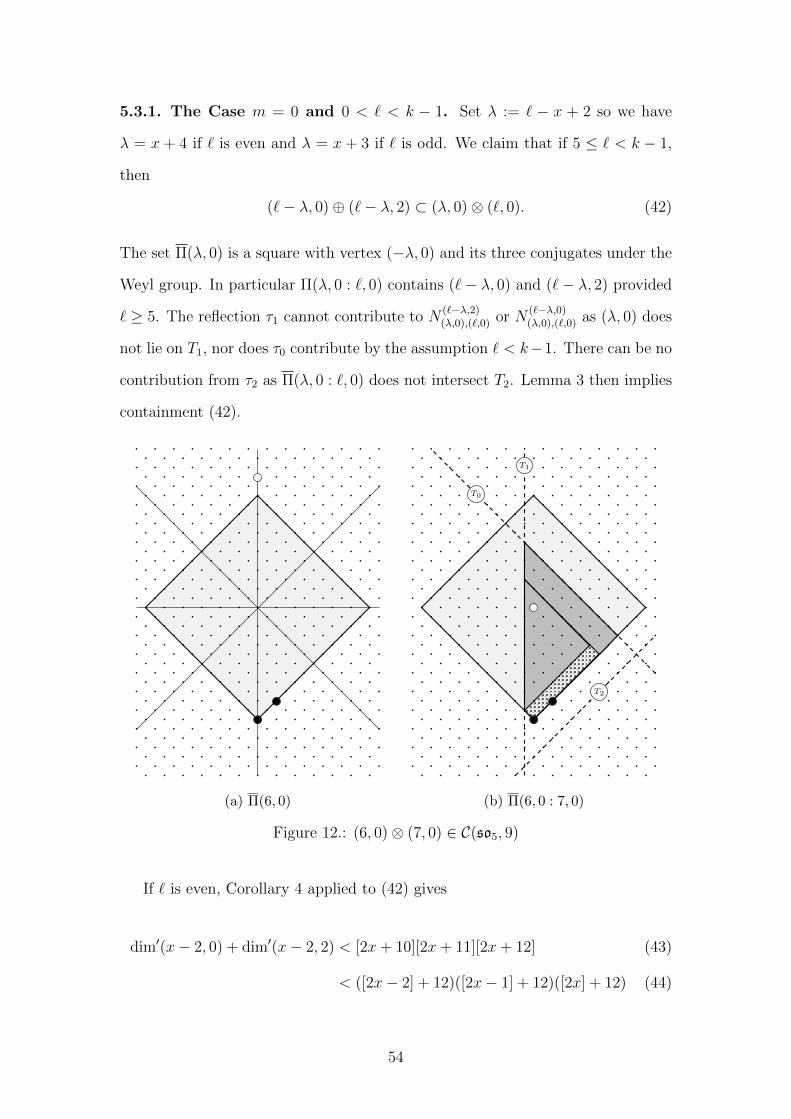
5.3.1. The Case m = 0 and 0 < ` < k − 1. Set λ := ` − x + 2 so we have

λ = x + 4 if ` is even and λ = x + 3 if ` is odd. We claim that if 5 ≤ ` < k − 1,

then

(`− λ, 0)⊕ (`− λ, 2) ⊂ (λ, 0)⊗ (`, 0). (42)

The set Π(λ, 0) is a square with vertex (−λ, 0) and its three conjugates under the

Weyl group. In particular Π(λ, 0 : `, 0) contains (`− λ, 0) and (`− λ, 2) provided

` ≥ 5. The reflection τ1 cannot contribute to N(`−λ,2)(λ,0),(`,0) or N

(`−λ,0)(λ,0),(`,0) as (λ, 0) does

not lie on T1, nor does τ0 contribute by the assumption ` < k−1. There can be no

contribution from τ2 as Π(λ, 0 : `, 0) does not intersect T2. Lemma 3 then implies

containment (42).

··················

··················

··················

··················

··················

··················

··················

··················

··················

··················

··················

··················

··················

··················

··················

··················

··················

··················

··················

··················

··················

··················

··················

··················

··················

··················

··················

(a) Π(6, 0)

··················

··················

··················

··················

··················

··················

··················

··················

··················

··················

··················

··················

··················

··················

··················

··················

··················

··················

··················

··················

··················

··················

··················

··················

··················

··················

··················

T1

T2

T0

(b) Π(6, 0 : 7, 0)

Figure 12.: (6, 0)⊗ (7, 0) ∈ C(so5, 9)

If ` is even, Corollary 4 applied to (42) gives

dim′(x− 2, 0) + dim′(x− 2, 2) < [2x+ 10][2x+ 11][2x+ 12] (43)

< ([2x− 2] + 12)([2x− 1] + 12)([2x] + 12) (44)

54

by applying Lemma 11 to the right-hand side of (43). Then expanding the product

on the right-hand side of (44) and subtracting the leading term (which is equal to

dim′(x− 2, 0)) from both sides yields

[3][2x− 2][2x+ 4][2x+ 1] < 24(6x2 + 30x+ 55) (45)

using Corollary 5 on the right-hand side to eliminate the quantum analogs. More-

over, applying Lemma 12 to the left-hand side of (45) (which is justified since

x = (1/2)`− 1 implies 2(2x+ 4) ≤ 2(k + 3)) leaves the inequalities

(` even)3

4(x− 1)(2x+ 1)(x+ 2) < 24(6x2 + 30x+ 55), and (46)

(` odd)3

4(x− 1)(2x+ 1)(x+ 2) < 120(x2 + 4x+ 6) (47)

repeating the same process for ` odd. Inequality (46) is true for even ` with

x ≤ 98 and inequality (47) is true for odd ` with x ≤ 81. The former is a

weaker bound on ` = 2x + 2 ≤ 198, which using θ(`, 0) = 1 by Lemma 8 implies

(2`2 + 6`)/(4(k + 3)) ∈ Z and thus k < (2(198)2 + 6(198))/4− 3 = 19896.

5.3.2. The Case 2 ≤ m ≤ x+ 2. Set λ := `+m− x so that λ = x+ 1 when `

is odd and λ = x+ 2 if ` is even. We claim that for 2 ≤ m ≤ x+ 2,

(x, 0)⊕ (x− 2, 2) ⊂ (λ, 0)⊗ (`,m). (48)

The set Π(λ, 0) is a square with vertex (−λ, 0) and its three conjugates under the

Weyl group. From the fact m ≥ 2 is even, the set Π(λ, 0 : `,m) contains (x, 0) and

(x − 2, 2). The square Π(λ, 0 : `,m) intersects T1 at 45 degree angles, thus (x, 0)

and (x − 2, 2) lying on this intersecting edge implies there is no contribution to

the desired fusion coefficients from τ1. Reflection τ0 could only contribute if (`,m)

lies on T0, and the assumption m ≤ x+ 2 ensures there is no contribution from τ2

as well. Lemma 3 then implies containment (48).

55

·····················

·····················

·····················

·····················

·····················

·····················

·····················

·····················

·····················

·····················

·····················

·····················

·····················

·····················

·····················

·····················

·····················

·····················

·····················

·····················

·····················

·····················

·····················

·····················

·····················

·····················

·····················

·····················

·····················

·····················

·····················

·····················

(a) Π(6, 0)

·····················

·····················

·····················

·····················

·····················

·····················

·····················

·····················

·····················

·····················

·····················

·····················

·····················

·····················

·····················

·····················

·····················

·····················

·····················

·····················

·····················

·····················

·····················

·····················

·····················

·····················

·····················

·····················

·····················

·····················

·····················

·····················

T1

T2

T0

(b) Π(6, 0 : 7, 4)

Figure 13.: (6, 0)⊗ (7, 4) ∈ C(so5, 12)

If ` is odd, Corollary 4 applied to (48) gives

dim′(x, 0) + dim′(x− 2, 2) < [2(x+ 2)][2(x+ 3)][2x+ 5] (49)

< ([2x+ 2] + 2)([2x+ 3] + 2)([2x+ 4] + 2) (50)

using Lemma 11 on the right-hand side of (49). Expanding the product on

the right-hand side of (50) and subtracting the leading term (which is equal to

dim′(x, 0)) yields

[3][2(x− 1)][2x+ 1][2(x+ 2)] < 24(x+ 2)2 (51)

using Corollary 5 on the right-hand side. Applying Lemma 12 to the left-hand

side of (51) is justified since 2(2x+ 4) = 2(`+m+ 3) ≤ 2(k + 3) and thus

(` odd)3

4(x− 1)(2x+ 1)(x+ 2) < 24(x+ 2)2, and (52)

(` even)3

4(x− 1)(2x+ 1)(x+ 2) < 24(2x2 + 10x+ 13). (53)

56

The inequality in (52) is true for odd ` with x ≤ 18 while the inequality in (53)

is true for even ` with x ≤ 35. Moreover 2 ≤ m ≤ 37, ` + m ≤ 72, and therefore

k < 2625 from Lemma 8 by maximizing (2`2 + 2`m+ 6`+m2 + 4m)/4− 3 subject

to these constraints.

5.3.3. The Case ` = 0 and m < k. We claim for m ≥ 4,

x−1⊕i=0

(i, 0) ⊂ (0,m)⊗ (0,m). (54)

The set Π(0,m) is a square with vertex (0,−m) and its three conjugates under

the Weyl group. In particular Π(0,m : 0,m) contains (i, 0) for 0 ≤ i ≤ x− 1. The

angles formed between T0, T2 and Π(0,m : 0,m) are 45 degrees, ensuring there is

no contribution to the desired fusion coefficients from τ0, τ2; Π(0,m : 0,m) does

not intersect T1 so there is no contribution from τ1 either. Lemma 3 then implies

containment (54).

·················

·················

·················

·················

·················

·················

·················

·················

·················

·················

·················

·················

·················

·················

·················

·················

·················

·················

·················

·················

·················

·················

·················

·················

·················

·················

·················

(a) Π(0, 10)

·················

·················

·················

·················

·················

·················

·················

·················

·················

·················

·················

·················

·················

·················

·················

·················

·················

·················

·················

·················

·················

·················

·················

·················

·················

·················

·················

T1

T2

T0

(b) Π(0, 10 : 0, 10)

Figure 14.: (0, 10)⊗ (0, 10) ∈ C(so5, 11)

57

Corollary 4 applied to (54) gives

x−1∑i=0

[2(i+ 1)][2(i+ 2)][2i+ 3] < [2][m+ 1][2(m+ 2)][m+ 3] (55)

⇒x−1∑i=0

(i+ 1)(i+ 2)(i+ 3/2) < 4(m+ 1)(m+ 2)(m+ 3) (56)

by applying Corollary 5 to the right-hand side of (55) and Lemma 12 to the left-

hand side of (55). Lemma 12 applies since m even implies 2(2x+ 2) = 2(m+ 4) <

2(k + 3). Now we rewrite the right-hand side of (56) in terms of x and re-index

the left-hand sum, observing each factor on the left-hand side of (56) is greater

than i to yieldx∑i=1

i3 < 4(2x+ 3)(2x+ 4)(2x+ 5). (57)

Using Faulhaber’s formula [28] on the left-hand side of (57) produces

1

4x2(x+ 1)2 < 4(2x+ 3)(2x+ 4)(2x+ 5)

which is true for x ≤ 131, and thus 2x + 2 = m ≤ 264. From Lemma 8 we have

θ(0,m) = 1, which implies (m2 + 4m)/(4(k + 3)) ∈ Z and thus k < (2642 + 4 ·

264)/4− 3 = 17685.

5.3.4. The Case 0 6= ` ≤ x < m− 2. Set λ := `+m− x+ 1 so that λ = x+ 3

if ` is even, and λ = x+ 2 if ` is odd. We claim if 0 6= ` ≤ x < m− 2, then

(`+ 1,m− λ)⊕ (`− 1,m− λ+ 2) ⊂ (0, λ)⊗ (`,m). (58)

The set Π(0, λ) is a square with vertex (0,−λ) and its seven conjugates under the

Weyl group. In particular Π(0, λ : `,m) contains (`+1,m−λ) and (`−1,m−λ+2)

since x+ 2 < m. The angles formed by Π(0, λ : `,m) and T2 are 45 degrees when

they exist which implies there is no contribution to the desired fusion coefficients

from τ2, while τ0 cannot contribute because (`,m) does not lie on T0. Lastly note

58

that Π(0, λ : `,m) does not intersect T1 since x + 2 < m so there can be no

contribution from τ1 either. Lemma 3 then implies containment (58).

·················

·················

·················

·················

·················

·················

·················

·················

·················

·················

·················

·················

·················

·················

·················

·················

·················

·················

·················

·················

·················

·················

·················

·················

·················

·················

(a) Π(0, 6)

·················

·················

·················

·················

·················

·················

·················

·················

·················

·················

·················

·················

·················

·················

·················

·················

·················

·················

·················

·················

·················

·················

·················

·················

·················

·················

T1

T2

T0

(b) Π(0, 6 : 3, 7)

Figure 15.: (0, 6)⊗ (3, 7) ∈ C(so5, 10)

Now notice that (`+ 1,m− λ) and (`− 1,m− λ+ 2) are contained in the set

of weights (s, t) ∈ Λ0 such that s+ t = x.

Lemma 13. If 0 ≤ x < k/2, dim′(0, x) ≤ dim′(s, x− s) for all 0 ≤ s ≤ x.

Proof. With κ := π/(2(k + 3)), define f(s) := sin((x− s + 1)κ) sin((x + s + 3)κ)

and g(s) := sin((2s+ 2)κ) so that

dim′(s, x− s) = sin−4(κ) sin(2(x+ 2)κ)f(s)g(s)

as a real function of s ∈ [0, x] with the constant sin−4(κ) sin(2(x+2)κ) > 0 since κ

and 2(x+2)κ are in the interval (0, π/2) for 0 ≤ x < k/2. We will prove our claim

by showing that (d2/ds2) dim′(s, x − s) < 0 on [0, x] and dim′(0, x) ≤ dim′(x, 0).

It can be easily verified that f(s) > 0, g(s) > 0, g′(s) > 0 and g′′(s) < 0 for

s ∈ [0, x], so we will explicitly compute with α := x− s+ 1 and β := x+ s+ 3 for

59

brevity:

f ′(s) = κ(sin(ακ) cos(βκ)− cos(ακ) sin(βκ))

= −κ sin(2(s+ 2)κ)

⇒ f ′′(s) = −2κ2 cos(2(s+ 2)κ).

The above computations imply f ′(s) < 0 and f ′′(s) < 0 for s ∈ [0, x]. Using the

product rule twice implies (fg)′′(s) < 0 and moreover (d2/ds2) dim′(s, x− s) < 0

since these functions differ by a positive constant factor.

Lastly we need to verify dim′(0, x) ≤ dim′(x, 0), or that

[2][x+ 1][x+ 3] ≤ [2x+ 2][2x+ 3]

⇔ [x+ 1][x+ 3] ≤ [2x+ 2]

[2][2x+ 3].

Note that

[2x+ 2]

[2]=qx+1 + q−(x+1)

q + q−1[x+ 1]

=

cos

((x+ 1)π

2(k + 3)

)cos

(π

2(k + 3)

) [x+ 1]

≥√

2

2[x+ 1],

because x+1 < (1/2)(k+3). Moreover we need only prove [x+3] ≤ (√

2/2)[2x+3].

This inequality is always true because x+3 and 2x+3 are in the interval (0, k+3)

and the function [n] = sin(nπ/(2(k + 3)))/ sin(π/(2(k + 3))) is strictly increasing

for n ∈ (0, k + 3).

60

Hence when ` is even, Lemma 13 and Corollary 4 applied to (58) implies

dim′(0, x) + dim′(0, x) ≤ dim′(`+ 1,m− λ) + dim′(`− 1,m− λ+ 2)

≤ dim′(0, x+ 3)

⇒ dim′(0, x) + dim′(0, x) < [2]([x+ 1] + 3)([2x+ 4] + 6)([x+ 3] + 3) (59)

by applying Lemma 11 to the right-hand side of (59). All terms in the inequality

in (59) have a factor of [2] which we divide out before expanding the product on

the right-hand side of (59) and subtracting the leading term (equal to dim′(0, x))

to yield

1

4(x+ 1)(x+ 2)(x+ 3) < 6(3x2 + 21x+ 38). (60)

Corollary 5 was applied eliminate the quantum analogs on the right-hand side of

(60) and Lemma 12 was applied to eliminate the quantum analogs on the left-hand

side, which is applicable since 4(x + 2) < 4(k + 3) since x < k/2. Inequality (60)

is true for x ≤ 72, which implies 0 < ` ≤ 72 and 74 < m ≤ 145. Moreover Lemma

8 implies k < 13319 by maximizing (2`2 + 2`m+ 6`+m2 + 4m)/4− 3 subject to

these constraints. Repeating the above with ` odd only changes the right-hand

side of (60) to 12(x+ 3)2, which clearly produces a more restrictive bound on x.

5.4. Proof of Theorem 5: C(g2, k)

Let A be a connected etale algebra in C(g2, k) with minimal nontrivial sum-

mand (`,m) (i.e. ` + (3/2)m is minimal) and fix x := d(1/2)(` + (3/2)m)e − 1;

the value x is the greatest integer n such that (n, 0) satisfies the hypotheses of

Lemma 9. Similarly one can set y := d(1/2)((2/3)` + m)e − 1; the value y is

the greatest integer n such that (0, n) satisfies the hypotheses of Lemma 9. The

proof of Theorem 5 will be split into four (clearly exhaustive) cases, illustrated by

example in Figure 16., with varying numbers of subcases for a fixed x: 0 ≤ ` ≤ 2,

3 ≤ ` ≤ x+ 3, x+ 3 < ` with m 6= 0, and m = 0.

61

·

·

·

·

·

·

·

·

·

·

·

·

·

·

·

·

·

·

·

·

·

·

·

·

·

·

·

·

·

·

·

·

·

·

·

·

·

·

·

·

·

·

·

·

·

·

·

·

·

·

·

·

·

·

·

·

·

·

·

·

·

·

·

·

·

·

·

·

·

·

·

·

·

·

·

·

·

·

·

·

·

·

·

·

·

·

·

·

·

·

·

·

·

·

·

·

·

·

·

·

·

·

·

·

·

·

·

·

·

·

·

·

·

·

·

·

·

·

·

·

·

·

·

·

·

·

·

·

·

·

·

·

·

·

·

·

·

·

·

·

·

·

·

·

·

·

·

·

·

·

·

·

·

·

·

·

·

·

·

·

·

·

·

·

·

·

·

·

·

·

·

·

·

·

·

·

·

·

·

·

·

·

·

·

·

·

·

·

·

·

·

·

·

·

·

·

·

·

·

·

·

·

·

·

·

·

·

·

·

·

·

·

·

·

·

·

·

·

·

·

·

·

·

·

·

·

·

·

·

·

·

·

·

·

·

·

·

·

·

·

·

·

·

·

·

·

·

·

·

·

·

·

·

·

·

·

·

·

·

·

·

·

·

·

·

·

·

·

·

·

·

·

·

·

·

·

·

·

·

·

·

·

·

·

·

·

·

·

·

·

·

·

·

·

·

·

·

·

·

·

·

·

·

·

·

·

·

·

·

·

·

·

·

·

·

·

·

·

·

·

·

·

·

·

·

·

·

·

·

·

·

·

·

·

·

·

·

·

·

·

·

·

·

·

·

·

·

·

·

·

·

·

·

·

·

·

·

·

·

·

·

·

·

·

·

·

·

·

·

·

·

·

·

·

·

·

·

·

·

·

·

·

·

·

·

·

·

·

·

·

·

·

·

·

·

·

·

·

·

·

·

·

·

·

·

·

·

·

·

·

·

·

·

·

·

·

·

·

·

·

·

·

·

·

·

·

·

·

·

·

·

·

·

·

·

·

·

·

·

·

·

·

·

·

·

·

·

·

·

·

·

·

·

·

·

·

·

·

·

·

·

·

·

·

·

·

·

·

·

·

·

·

·

·

·

·

·

·

·

·

·

·

·

·

·

·

·

·

·

·

·

·

·

·

·

·

·

·

·

·

·

·

·

·

·

·

·

·

·

·

T1

T0

T2

Figure 16.: Possible (`,m) when k = 20 and x = 5

5.4.1. The Case 0 ≤ ` ≤ 2.

The Subcase ` = 0. We will employ the same strategy as Section 5.3.1.. Recall

y = dm/2e − 1 if ` = 0 and set λ := m− y + 1 so that λ = y + 3 if m is even, and

λ = y + 2 if m is odd. We claim for 4 < m ≤ k/2,

(0, y − 1)⊕ (3, y − 2) ⊂ (0, λ)⊗ (0,m). (61)

The set Π(0, λ), illustrated by example in Figure 17., (refer to Section 3.1. for

descriptions of the notation and visualization used), is a hexagon with vertex

(0,−λ) and its five conjugates under the Weyl group. In particular Π(0, λ : 0,m)

contains (0, y−1) and (3, y−2) since m > 4. There is no contribution to N(0,y−1)(0,λ),(0,m)

or N(3,y−2)(0,λ),(0,m) from τ2 because the angles formed by Π(0, λ : 0,m) and T2 are

60 degrees and there is no contribution from τ1 because the angles formed by

Π(0, λ : 0,m) and T1 (when they exist) are 30 degrees. There is no contribution

62

from τ0 because (0,m) does not lie on T0. Lemma 3 then implies containment

(61).

················

················

················

················

················

················

················

················

················

················

················

················

················

················

················

················

················

················

················

················

················

················

················

················

················

················

················

················

················

················

················

················

················

················

················

················

················

················

················

················

················

················

················

················

················

················

················

················

················

(a) Π(0, 5)

················

················

················

················

················

················

················

················

················

················

················

················

················

················

················

················

················

················

················

················

················

················

················

················

················

················

················

················

················

················

················

················

················

················

················

················

················

················

················

················

················

················

················

················

················

················

················

················

················

T1

T0

T2

(b) Π(0, 5 : 0, 6)

Figure 17.: (0, 5)⊗ (0, 6) ∈ C(g2, 18)

If m is even, Corollary 4 applied to (61) gives

dim′(0, y − 1) + dim′(3, y − 2) (62)

≤ [3y + 12][3y + 15][6y + 27][3y + 13][3y + 14] (63)

≤ ([3y] + 12)([3y + 3] + 12)([6y + 3] + 24)([3y + 1] + 12)([3y + 2] + 12) (64)

where (64) is gained by applying Corollary 5 to (63). Expanding the product in

(64) and subtracting the leading term (equal to dim′(0, y − 1)) yields

27

8(y − 1)(y + 3)(y + 1)(3y + 1)(3y + 5) ≤ 3240(3y4 + 30y3 + 136y2 + 305y + 273)

by applying Lemma 12 to the factors of dim′(3, y−2) in (62), which is true for even

m with y ≤ 324 or likewise m ≤ 650. From Lemma 8, θ(0,m) = 1 which implies

(3m2+9m)/(3(k+4)) ∈ Z and moreover k ≤ (1/3)(3(650)2+9(650))−4 = 424446.

63

By repeating the above argument with m odd we obtain the inequality

27

8(y − 1)(y + 3)(y + 1)(3y + 1)(3y + 5) < 810(9y4 + 72y3 + 255y2 + 444y + 308)

which is true for y ≤ 242 which evidently yields a stricter bound on k.

The Subcase ` = 1. The strategy is identical to Section 5.4.1., except with

λ := m− y + 1 we claim

(0, y − 1)⊕ (3, y − 2) ⊂ (1, λ)⊗ (0,m),

and we omit the redundant arguments for both this containment and to produce

the following inequalities, based on m being even or odd, respectively:

27

32y(y + 1)(2y + 1)(3y + 1)(3y + 2) ≤ 324(54y4 + 613y3 + 2861y2 + β1y + β2)

27

32y(y + 1)(2y + 1)(3y + 1)(3y + 2) ≤ 1620(y + 3)(9y3 + 65y2 + 183y + 191)

where β1 = 6427 and β2 = 5725 for display purposes. The first inequality is true

for even m with y ≤ 1160 and the second for odd m with y ≤ 967, hence m ≤ 2322

and moreover k ≤ (12 + 3(1)(2322) + 5(1) + 3(2322)2 + 9(2322))/3− 4 = 5400970.

The Subcase ` = 2. The strategy is identical to Section 5.4.1., except with

λ := m− y + 1 we claim

(0, y − 1)⊕ (3, y − 2) ⊂ (2, λ)⊗ (0,m),

and so we omit the redundant argument to produce the following inequalities,

based on m being even or odd, respectively:

27

32y(y + 1)(2y + 1)(3y + 1)(3y + 2) ≤ 81(399y4 + 5171y3 + β1y

2 + β2y + β3)

27

32y(y + 1)(2y + 1)(3y + 1)(3y + 2) ≤ 2835(y + 3)(9y3 + 73y2 + 234y + 278)

64

where β1 = 28239, β2 = 74821, and β3 = 78570 for display purposes. The first

inequality is true for even m with y ≤ 2138 and the second for odd m with

y ≤ 1688, hence m ≤ 4272 and moreover k ≤ (22 + 3(2)(4272) + 5(2) + 3(4272)2 +

9(4272))/3− 4 < 18271135.

5.4.2. The Case m = 0. Recall x = d`/2e − 1 if m = 0. Set λ := ` − x + 1 so

that λ = x+ 3 if ` is even and λ = x+ 2 if ` is odd. We claim that for 4 < ` ≤ k,

(x− 1, 0)⊕ (x− 2, 1) ⊂ (λ, 0)⊗ (`, 0). (65)

The set Π(λ, 0), illustrated by example in Figure 18., is a hexagon with vertex

(−λ, 0) and its five conjugates under the Weyl group. In particular Π(λ, 0 : `, 0)

contains (x−1, 0) and (x−2, 1) provided ` > 4. The angles formed by Π(λ, 0 : `, 0)

and T1 are 30 degrees and the angles formed by Π(λ, 0 : `, 0) and T0, T2 are 60

degrees, ensuring there can be no contribution from τ0, τ1, τ2. Lemma 3 then

implies containment (65).

················

················

················

················

················

················

················

················

················

················

················

················

················

················

················

················

················

················

················

················

················

················

················

················

················

················

················

················

················

················

················

················

················

················

················

················

················

················

················

················

················

················

················

················

················

················

················

················

················

(a) Π(9, 0)

················

················

················

················

················

················

················

················

················

················

················

················

················

················

················

················

················

················

················

················

················

················

················

················

················

················

················

················

················

················

················

················

················

················

················

················

················

················

················

················

················

················

················

················

················

················

················

················

················

T2

T0

T1

(b) Π(9, 0 : 15, 0)

Figure 18.: (9, 0)⊗ (15, 0) ∈ C(g2, 20)

65

If m is even, Corollary 4 applied to (65) gives

dim′(x− 1, 0) + dim′(x− 2, 1) (66)

≤ [x+ 4][3][3x+ 15][3x+ 18][x+ 7][2x+ 11] (67)

≤ ([x] + 4)[3]([3x+ 3] + 12)([3x+ 6] + 12)([x+ 3] + 4)([2x+ 3] + 8) (68)

where (68) is gained by applying Corollary 5 to (67). Expanding the product in

(68) and subtracting the leading term (which is equal to dim′(x− 1, 0)) yields

27

16(x−1)(x+ 2)(x+ 3)(x+ 5)(x+ 2) ≤ 1080(x4 + 14x3 + 80x2 + 217x+ 231) (69)

by applying Lemma 12 to the factors of dim′(x − 2, 1) in (66), which is true

for even x ≤ 642 or likewise ` ≤ 1286. From Lemma 8 we know θ(`, 0) = 1

which implies (`2 + 5`)/(3(k + 4)) ∈ Z and with the proven bound on `, k ≤

(1/3)((1286)2 + 5(1286))− 4 = 1660214/3 < 553405.

If m is odd, the above process yields the inequality

27

16(x− 1)(x+ 2)(x+ 3)(x+ 5)(x+ 2) ≤ 810(x+ 3)2(x2 + 6x+ 12)

which is true for x ≤ 481 which evidently yields a stricter bound on k.

5.4.3. The Case 3 ≤ ` ≤ x + 3. We will employ the same strategy as Section

5.3.2. but the proof is necessarily split based on ` modulo 3.

The Subcase ` ≡ 0 (mod 3). Recall y = d(1/2)((2/3)` + m)e − 1 and set

λ := (2/3)`+m− y so that λ = y + 2 if m is even and λ = y + 1 if m is odd. We

claim

(0, y)⊕ (3, y − 2) ⊂ (0, λ)⊗ (`,m). (70)

The set Π(0, λ), illustrated by example in Figure 19., is a hexagon with vertex

(0,−λ) and its five conjugates under the Weyl group. In particular Π(0, λ : `,m)

66

contains (0, y) and (3, y − 2). To see this, Π(0, λ : `,m) contains more generally

all (`− 3i,m− λ+ 2i) for all 0 ≤ i ≤ (1/3)`. The angles formed by Π(0, λ : `,m)

and T1 are 30 degrees and the angles formed by Π(0, λ : `,m) and T2 are 60

degrees, implying there are no contributions from τ1, τ2. The angles formed by

Π(0, λ : `,m) and T0 are 90 (or 30) degrees when they exist, but since (0,m) does

not lie on T0 there is no contribution from τ0. Lemma 3 then implies containment

(70).

················

················

················

················

················

················

················

················

················

················

················

················

················

················

················

················

················

················

················

················

················

················

················

················

················

················

················

················

················

················

················

················

················

················

················

················

················

················

················

················

················

················

················

················

················

················

················

················

················

(a) Π(0, 4)

················

················

················

················

················

················

················

················

················

················

················

················

················

················

················

················

················

················

················

················

················

················

················

················

················

················

················

················

················

················

················

················

················

················

················

················

················

················

················

················

················

················

················

················

················

················

················

················

················

T1

T0

T2

(b) Π(0, 4 : 3, 4)

Figure 19.: (0, 4)⊗ (3, 4) ∈ C(g2, 15)

If m is even, Corollary 4 applied to (70) gives

dim′(0, y) + dim′(3, y − 2) (71)

≤ [3y + 9][3y + 12][6y + 21][3y + 10][3y + 11] (72)

≤ ([3y + 3] + 6)([3y + 6] + 6)([6y + 9] + 18)([3y + 4] + 6)([3y + 5] + 6) (73)

by applying Corollary 5 to (72). Expanding the product in (73) and subtracting

the leading term (equal to dim′(0, y)) yields

27

8(y− 1)(y+ 3)(y+ 1)(3y+ 1)(3y+ 5) ≤ 1620(y2 + 5y+ 8)(3y2 + 15y+ 19) (74)

67

which is true for even (2/3)`+m with y ≤ 164. This bound implies `+ (3/2)m ≤

495. From Lemma 8 we know θ(`,m) = 1 which implies k ≤ (1/3)(`2 + 3`m +

5`+ 3m2 + 9m)− 4; and for `+ (3/2)m ≤ 495 we have k ≤ 109886. As in Sections

5.4.1. and 5.4.2., the case in which `+ (3/2)m is odd leads to a stricter bound on

k by this method.

The Subcase ` ≡ 1 (mod 3). With y = d(1/2)((2/3)` + m)e − 1, we set λ :=

(2/3)(`− 1) + m− y. This implies λ = y if m is even and λ = y + 1 if m is odd.

We claim

(0, y)⊕ (3, y − 2) ⊂ (1, λ)⊗ (`,m) (75)

and we omit the argument for this containment as it is identical to that of Section

5.4.3..

If m is odd, Corollary 4 applied to (75) gives

dim′(0, y) + dim′(3, y − 2) (76)

≤ [2][3y + 6][3y + 12][6y + 18][3y + 8][3y + 10] (77)

≤ [4]([3y − 3] + 9)([3y + 9] + 3)([6y + 6] + 12)([3y + 1] + 7)([3y + 5] + 5) (78)

by applying Corollary 5 to the right-hand side of (77). Expanding the product on

the right-hand side of (78) and subtracting the leading term (equal to dim′(0, y))

yields

27

8(y−1)(y+3)(y+1)(3y+1)(3y+5) ≤ 648(y+3)(12y3−20y2−282y−425) (79)

which is true for y ≤ 252. Hence we have (2/3)` + m ≤ 1288 and furthermore

`+(3/2)m ≤ 1933. The level k is bounded under these constraints by k ≤ 1664094.

As in Sections 5.4.1. and 5.4.2., the case in which m is even leads to a stricter

bound on k by this method.

68

The Subcase ` ≡ 2 (mod 3). With y = d(1/2)((2/3)` + m)e − 1, we set λ :=

(2/3)(`− 2) + m− y. This implies λ = y if m is even and λ = y − 1 if m is odd.

We claim

(0, y)⊕ (3, y) ⊂ (2, λ)⊗ (`,m) (80)

and we omit the argument for this containment as it is identical to that of Section

5.4.3..

If m is even, Corollary 4 applied to (80) gives

dim′(0, y) + dim′(3, y − 2) (81)

≤ [3][3y + 3][3y + 12][6y + 15][3y + 6][3y + 9] (82)

≤ [4]([3y − 3] + 6)([3y + 9] + 3)([6y + 6] + 9)([3y + 1] + 5)([3y + 5] + 4) (83)

by applying Corollary 5 to (77). Expanding the product in (78) and subtracting

the leading term (which is equal to dim(0, x)) yields

27

8(y− 1)(y+ 3)(y+ 1)(3y+ 1)(3y+ 5) ≤ 540(y+ 3)(y+ 1)(27y2 + 88y+ 74) (84)

which is true for y ≤ 962, hence (2/3)` + m ≤ 1926 and moreover ` + (3/2)m ≤

2889. This produces a bound of k ≤ 3715250. As in Sections 5.4.1. and 5.4.2., the

case in which m is odd leads to a stricter bound on k by this method.

5.4.4. The Case x + 3 < ` and m 6= 0. We will employ a similar strategy to

Section 5.3.4.. We first claim that if x + 3 < `, then for some x + 1 ≤ λ ≤ x + 3,

(λ, 0)⊗ (`,m) contains two summands (s, t) such that s + (3/2)t = x, depending

on the parity of ` and remainder of m modulo 4. We will provide proof of this

claim in the most extreme case ` is even and 4 | m, using λ = x + 3, leaving the

other near identical cases to the reader. The only changes in each case are due

to the slight differences caused by the ceiling function in the definition of x. Note

that under our current assumptions x = (1/2)`+ (3/4)m− 1.

The set Π(λ, 0), illustrated by example in Figure 20., is a hexagon with vertex

69

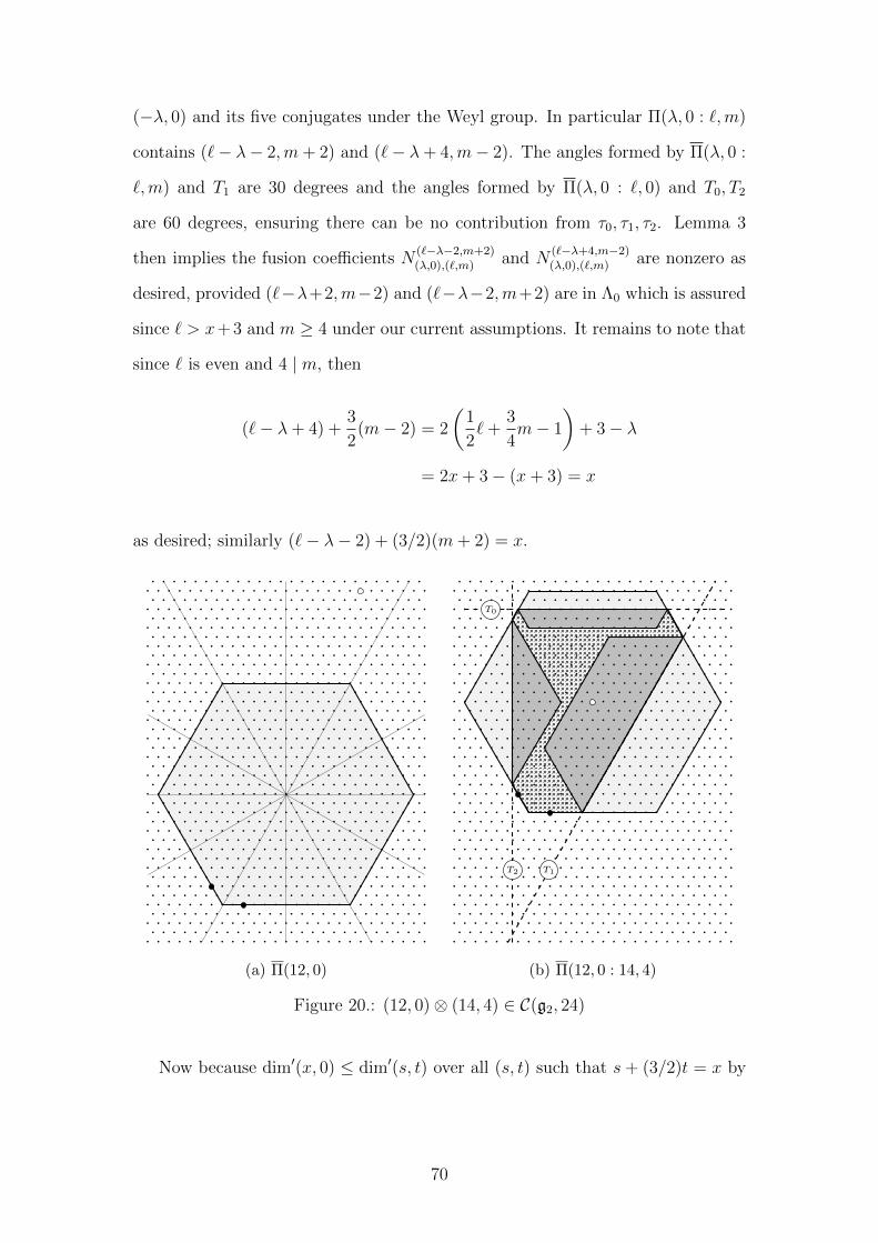
(−λ, 0) and its five conjugates under the Weyl group. In particular Π(λ, 0 : `,m)

contains (`− λ− 2,m+ 2) and (`− λ+ 4,m− 2). The angles formed by Π(λ, 0 :

`,m) and T1 are 30 degrees and the angles formed by Π(λ, 0 : `, 0) and T0, T2

are 60 degrees, ensuring there can be no contribution from τ0, τ1, τ2. Lemma 3

then implies the fusion coefficients N(`−λ−2,m+2)(λ,0),(`,m) and N

(`−λ+4,m−2)(λ,0),(`,m) are nonzero as

desired, provided (`−λ+2,m−2) and (`−λ−2,m+2) are in Λ0 which is assured

since ` > x+ 3 and m ≥ 4 under our current assumptions. It remains to note that

since ` is even and 4 | m, then

(`− λ+ 4) +3

2(m− 2) = 2

(1

2`+

3

4m− 1

)+ 3− λ

= 2x+ 3− (x+ 3) = x

as desired; similarly (`− λ− 2) + (3/2)(m+ 2) = x.

····················

····················

····················

····················

····················

····················

····················

····················

····················

····················

····················

····················

····················

····················

····················

····················

····················

····················

····················

····················

····················

····················

····················

····················

····················

····················

····················

····················

····················

····················

····················

····················

····················

····················

····················

····················

····················

····················

····················

····················

····················

····················

····················

····················

····················

····················

····················

····················

····················

····················

····················

····················

····················

(a) Π(12, 0)

····················

····················

····················

····················

····················

····················

····················

····················

····················

····················

····················

····················

····················

····················

····················

····················

····················

····················

····················

····················

····················

····················

····················

····················

····················

····················

····················

····················

····················

····················

····················

····················

····················

····················

····················

····················

····················

····················

····················

····················

····················

····················

····················

····················

····················

····················

····················

····················

····················

····················

····················

····················

····················

T2

T0

T1

(b) Π(12, 0 : 14, 4)

Figure 20.: (12, 0)⊗ (14, 4) ∈ C(g2, 24)

Now because dim′(x, 0) ≤ dim′(s, t) over all (s, t) such that s + (3/2)t = x by

70

the same reasoning that lead to Lemma 13, Corollary 4 implies

dim′(x, 0) + dim′(x, 0) (85)

≤ [x+ 4][3][3x+ 15][3x+ 18][x+ 7][2x+ 11] (86)

< ([x+ 1] + 3)[3]([3x+ 6] + 9)([3x+ 9] + 9)([x+ 4] + 3)([2x+ 5] + 6) (87)

by applying Corollary 5 to (86). Expanding the product in (87) and subtracting

the leading term (equal to dim′(x, 0)) from both sides of this equality yields

27

64(x+ 1)(x+ 2)(x+ 3)(x+ 4)(2x+ 5) < 810(x+ 4)2(x2 + 8x+ 19) (88)

by applying Lemma 12 to the factors on the left-hand side of (88) and Corollary

5 to the factors on the right-hand side of (88). The inequality in (88) is true for

x ≤ 963. Moreover ` ≤ 1926 and m ≤ 963, therefore k ≤ (1/3)(`2 + 3`m + 5` +

3m2 + 9m)− 4 is maximized within these bounds at k ≤ 4023089.

71

REFERENCES CITED

[1] Henning Haahr Andersen and Jan Paradowski. Fusion categories arisingfrom semisimple Lie algebras. Communications in Mathematical Physics,(169):563–588, 1995.

[2] F. A. Bais and Peter Bouwknegt. A classification of subgroup truncations ofthe bosonic string. Nuclear Physics, 279:561–570, 1987.

[3] Bojko Bakalov and Jr. Alexander Kirillov. Lectures on Tensor Categoriesand Modular Functors, volume 21 of University Lecture Series. AmericanMathematical Society, 2001.

[4] Jens Bockenhauer, David E. Evans, and Yasuyuki Kawahigashi. On α-induction, chiral generators and modular invariants for subfactors. Com-munications in Mathematical Physics, 208(2):429–487, 1999.

[5] Jens Bockenhauer, David E. Evans, and Yasuyuki Kawahigashi. Chiral struc-ture of modular invariants for subfactors. Communications in MathematicalPhysics, 210(3):733–784, 2000.

[6] Paul Bruillard, Siu-Hung Ng, Eric C. Rowell, and Zhenghan Wang. On clas-sification of modular categories by rank. International Mathematics ResearchNotices, 2016.

[7] Alfredo Cappelli, Claude Itzykson, and J. B. Zuber. The A-D-E classifica-

tion of minimal and A(1)1 conformal invariant theories. Communications in

Mathematical Physics, 113(1):1–26, 1987.

[8] Robert Coquereaux, Rochdi Rais, and El Hassan Tahri. Exceptional quantumsubgroups for the rank two Lie algebras B2 and G2. Journal of MathematicalPhysics, 51(092302), 2010.

[9] Robert Coquereaux and Gil Schieber. Quantum symmetries for exceptionalSU(4) modular invariants associated with conformal embeddings. Symmetry,Integrability and Geometry: Methods and Applications, 5(044), 2009.

[10] Alexei Davydov, Michael Muger, Dmitri Nikshych, and Victor Ostrik. TheWitt group of nondegenerate braided fusion categories. Journal fur die reineund angewandte Mathematik (Crelles Journal), (677):135–177, 2013.

[11] Alexei Davydov, Dmitri Nikshych, and Victor Ostrik. On the structure of theWitt group of braided fusion categories. Selecta Mathematica, (19):237–269,2013.

[12] Pierre Deligne. Categories tannakiennes. Progressions in Mathematics,(87):111–195, 1990.

[13] Pierre Deligne. Categories tensorielles. Moscow Mathematics Journal,(2):227–248, 2002.

72

[14] Vladimir Drinfeld, Shlomo Gelaki, Dmitri Nikshych, and Victor Ostrik. Onbraided fusion categories I. Selecta Mathematica, (16):1–119, 2010.

[15] Sebas Eliens. Anyon condensation: Topological symmetry breaking phasetransitions and commutative algebra objects in braided tensor categories.Master’s thesis, Universiteit van Amsterdam, Netherlands, 2010.

[16] Nikshych Dmitri Etingof, Pavel and Victor Ostrik. On fusion categories.Annals of Mathematics, 162(2):581–642, 2005.

[17] Pavel Etingof, Shlomo Gelaki, Dmitri Nikshych, and Victor Ostrik. TensorCategories:. Mathematical Surveys and Monographs. American MathematicalSociety, 2015.

[18] Mikhail Finkelberg. An equivalence of fusion categories. Geometric Func-tional Analysis, 6:249–267, 1996.

[19] Jurgen Fuchs, Ingo Runkel, and Christoph Schweigert. TFT construction ofRCFT correlators I: partition functions. Nuclear Physics B, 646(3):353 – 497,2002.

[20] Jurgen Fuchs and Christoph Schweigert. Consistent systems of correlators innon-semisimple conformal field theory. Advances in Mathematics, 307:598 –639, 2017.

[21] Jurgen Fuchs, Christoph Schweigert, and Alessandro Valentino. Bicategoriesfor boundary conditions and for surface defects in 3-D TFT. Communicationsin Mathematical Physics, 321(2):543–575, 2013.

[22] Terry Gannon. The classification of SU(3) modular invariants revisited. An-nales de l’institut Henri Poincar (A) Physique thorique, 65(1):15–55, 1996.

[23] Pinhas Grossman and Noah Snyder. Quantum subgroups of the Haagerupfusion categories. Communications in Mathematical Physics, 311(3):617–643,2012.

[24] Yi-Zhi Huang, Alexander Kirillov, and James Lepowsky. Braided tensor cat-egories and extensions of vertex operator algebras. Communications in Math-ematical Physics, 337(3):1143–1159, 2015.

[25] James E. Humphreys. Introduction to Lie Algebras and Representation The-ory. Graduate Texts in Mathematics. Springer, 1972.

[26] Andre Joyal and Ross Street. Braided tensor categories. Advances in Math-ematics, 102:20–78, 1993.

[27] Alexandre Kirillov and Victor Ostrik. On a q-analogue of the Mckay corre-spondence and the ADE classification of sl2 conformal field theories. Advancesin Mathematics, 171:183–227, 2002.

[28] Donald E. Knuth. Johann Faulhaber and sums of powers. Mathematics ofComputation, 61(203):277–294, 1993.

73

[29] Liang Kong. Anyon condensation and tensor categories. Nuclear Physics B,886:436–482, 2014.

[30] Gregory Moore and Nathan Seiberg. Lectures on RCFT. Superstrings ’89,1:1–129, 1989.

[31] Michael Muger. From subfactors to categories and topology II: The quantumdouble of tensor categories and subfactors. Journal of Pure and AppliedAlgebra, 180(1-2):159–219, 2003.

[32] Michael Muger. On the structure of modular categories. Proceedings of theLondon Mathematical Society, (87):291–308, 2003.

[33] Victor Ostrik. Fusion categories of rank 2. Mathematical Research Letters,10:177–183, 2003.

[34] Victor Ostrik. Module categories over the drinfeld double of a finite group.International Mathematics Research Notices, 2003(27):1507–1520, 2003.

[35] Victor Ostrik. Module categories, weak Hopf algebras and modular invariants.Transformation Groups, 8(2):177–206, 2003.

[36] Victor Ostrik. Pivotal fusion categories of rank 3. Moscow MathematicalJournal, 15(2):373–396, 2015.

[37] Bodo Pareigis. On braiding and dyslexia. Journal of Algebra, (171):413–425,1995.

[38] Stephen Sawin. Closed subsets of the Weyl alcove and TQFTs. PacificJournal of Mathematics, 228(2):305–324, 2006.

[39] Stephen Sawin. Quantum groups at roots of unity and modularity. Journalof Knot Theory and Its Ramifications, (15):1245–1277, 2006.

[40] Andre Schellekens and N. Warner. Conformal subalgebras of Kac-Moodyalgebras. Physical Review D, 34:3092–3096, 1986.

[41] Andrew Schopieray. Classification of sl3 relations in the Witt group of nonde-generate braided fusion categories. Communications in Mathematical Physics,353(3):1103–1127, 2017.

[42] Andrew Schopieray. Level bounds for exceptional quantum subgroups in ranktwo. submitted for publication, 2017.

74