relational databases, logic, and complexity
TRANSCRIPT
1
Relational Databases, Logic, and Complexity
Phokion G. Kolaitis
University of California, Santa Cruz
&
IBM Research-Almaden
2009 GII Doctoral School on Advances in Databases
2
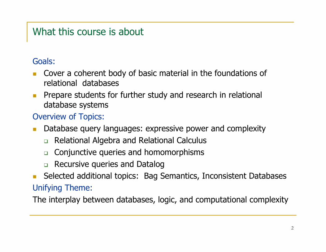
What this course is about
Goals:
� Cover a coherent body of basic material in the foundations of relational databases
� Prepare students for further study and research in relational database systems
Overview of Topics:
� Database query languages: expressive power and complexity
� Relational Algebra and Relational Calculus
� Conjunctive queries and homomorphisms
� Recursive queries and Datalog
� Selected additional topics: Bag Semantics, Inconsistent Databases
Unifying Theme:
The interplay between databases, logic, and computational complexity
3
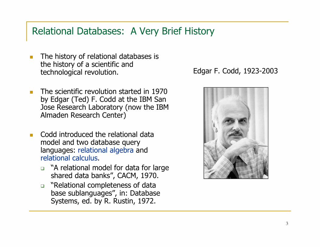
Relational Databases: A Very Brief History
� The history of relational databases is the history of a scientific and technological revolution.
� The scientific revolution started in 1970 by Edgar (Ted) F. Codd at the IBM San Jose Research Laboratory (now the IBM Almaden Research Center)
� Codd introduced the relational data model and two database query languages: relational algebra and relational calculus.
� “A relational model for data for large shared data banks”, CACM, 1970.
� “Relational completeness of data base sublanguages”, in: Database Systems, ed. by R. Rustin, 1972.
Edgar F. Codd, 1923-2003

4
Relational Databases: A Very Brief History
� Researchers at the IBM San Jose Laboratory embark on the
System R project, the first implementation of a relational database management system (RDBMS)
� In 1974-1975, they develop SEQUEL, a query language that eventually became the industry standard SQL.
� System R evolved to DB2 – released first in 1983.
� M. Stonebraker and E. Wong embark on the development of the Ingres RDBMS at UC Berkeley in 1973.
� Ingres is commercialized in 1983; later, it became PostgreSQL, a free software OODBMS (object-oriented DBMS).
� L. Ellison founds a company in 1979 that eventually becomes Oracle Corporation; Oracle V2 is released in 1979 and Oracle V3 in 1983.
� Ted Codd receives the ACM Turing Award in 1981.

5
Relational Database Industry Today
� According to Gartner, Inc., June 2007:
“Worldwide relational database management systems (RDBMS) total software revenue totaled $15.2 billion in 2006, a 14.2 percent increase from 2005 revenue of $13.3 billion.”
� In 2007, the total RDBMS software revenue increased to $17.1 billion (figures released in July 2008).
100%15.2BTotal
7.8%1.2BOther
3.2%486.7MSybase
3.2%494.2MTeradata
17.4%2.654BMicrosoft
21.1%3.204BIBM
47.1%7.168BOracle
2006 Market Share
2006 Revenue
Company

6
Database Research Today
� A very vibrant community comprising several thousand researchersaround the world.
� Several major annual conferences in database research:
� SIGMOD, PODS, VLDB, ICDE, EDBT, ICDT (top six).
� Numerous other conferences and workshops.
� Several major scholarly journals dedicated to database research:
� ACM TODS, VLDB Journal, IEEE TKDE, …
� Strong database research groups in academia around the world.
� Several database research groups in industrial laboratories.

7
Database Management Systems
A database management system (DBMS) provides support for:
� At least one data model (a mathematical abstraction for representing data);
� At least one high level data language (language for defining, updating, manipulating, and retrieving data);
� Transaction management & concurrency control mechanisms;
� Access control (limit access of certain data to certain users);
� Resiliency (ability to recover from crashes).

8
Data Models and Data Languages
� A data model is a mathematical formalism for describing and representing data.
� A data model is accompanied by a data language that has two parts: a data definition language and a data manipulation language.
� A data definition language (DDL) has a syntax for describing “database templates” in terms of the underlying data model.
� A data manipulation language (DML) supports the following operations on data:
� Insertion
� Deletion
� Update
� Retrieval and extraction of data (query the data).
� The first three operations are fairly standard. However, there is much variety on data retrieval and extraction (query languages).

9
The Relational Data Model (E.F. Codd – 1970)
� The Relational Data Model uses the mathematical concept of a relation as the formalism for describing and representing data.
� Question: What is a relation?
� Answer:
� Formally, a relation is a subset of a cartesian product of sets.
� Informally, a relation is a “table” with rows and columns.

10
The Relational Data Model (E.F. Codd – 1970)
� The Relational Data Model uses the mathematical concept of a relation as the formalism for describing and representing data.
� Question: What is a relation?
� Answer:
� Formally, a relation is a subset of a cartesian product of sets.
� Informally, a relation is a “table” with rows and columns.
…………
$11,245.75Hull10992-35671Hawthorne
$3,567.53Abiteboul10991-06284Orsay
balancecustomer-nameaccount-nobranch-name
CHECKING-ACCOUNT Table

11
Basic Notions from Discrete Mathematics
� A k-tuple is an ordered sequence of k objects (need not be distinct)
� (2,0,1) is a 3-tuple; (a,b,a,a,c) is a 5-tuple, and so on.
� If D1, D2, …, Dk are k sets, then the cartesian product
D1 × D2 … × Dk of these sets is the set of all k-tuples
(d1,d2, …,dk) such that di ∈ Di, for 1 ≤ i ≤ k.
� Fact: Let |D| denote the cardinality (= # of elements) of a set D. Then |D1 × D2 × … × Dk| = |D1|× |D2| × …× |Dk|.
� Example: If D1 = {0,1} and D2 ={a,b,c,d}, then |D1|×|D2| = 8.
� Warning: Computing cartesian products is an expensive operation!

12
Basic Notions from Discrete Mathematics
� A k-ary relation R is a subset of a cartesian product of k sets, i.e.,
� R ⊆ D1× D2× … × Dk.
� Examples:
� Unary R = {0,2,4,…,100} (R ⊆ D)
� Binary T = {(a,b): a and b have the same birthday}
� Ternary S = {(m,n,s): s = m+n}
� …
13
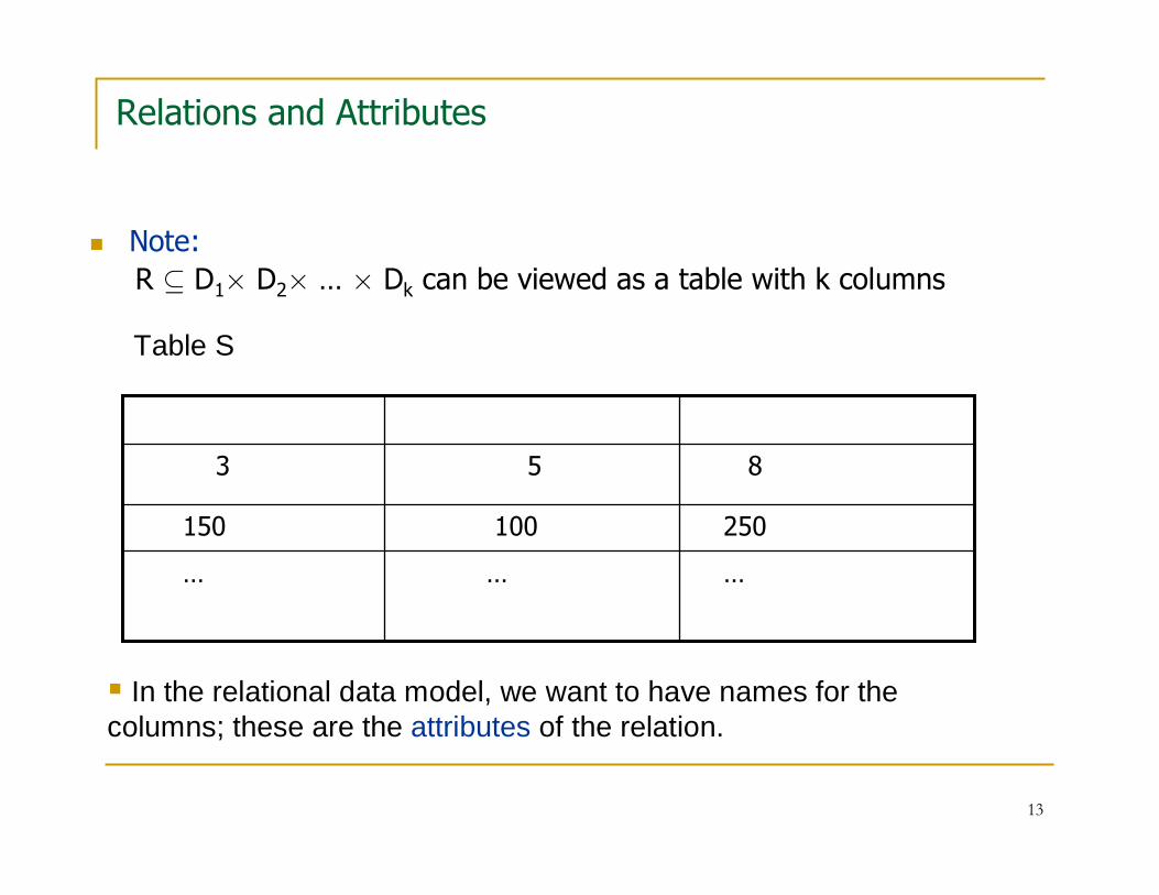
Relations and Attributes
� Note:
R ⊆ D1× D2× … × Dk can be viewed as a table with k columns
………
250100150
853
Table S
� In the relational data model, we want to have names for the columns; these are the attributes of the relation.

14
Relation Schemas and Relational Database Schemas
� A k-ary relation schema R(A1,A2,…,AK) is a set {A1,A2,…,Ak} of
k attributes.
� COURSE(course-no, course-name, term, instructor, room, time)
� CITY-INFO(name, state, population)
Thus, a k-ary relation schema is a “blueprint”, a “template” for some
k-ary relation.
� An instance of a relation schema is a relation conforming to the schema (arities match; also, in DBMS, data types of attributes match).
� A relational database schema is a set of relation schemas Ri(A1,A2,…,Aki),
for 1≤ i≤ m.
� A relational database instance of a relational schema is a set of relations Ri
each of which is an instance of the relation schema Ri, 1≤ i≤ m.

15
Relational Database Schemas - Examples
� BANKING relational database schema with relation schemas
� CHECKING-ACCOUNT(branch, acc-no, cust-id, balance)
� SAVINGS-ACCOUNT(branch, acc-no, cust-id, balance)
� CUSTOMER(cust-id, name, address, phone, email)
� ….
� UNIVERSITY relational database schema with relation schemas
� STUDENT(student-id, student-name, major, status)
� FACULTY(faculty-id, faculty-name, dpt, title, salary)
� COURSE(course-no, course-name, term, instructor)
� ENROLLS(student-id, course-no, term)
� …

16
Schemas vs. Instances
Keep in mind that there is a clear distinction between
� relation schemas and instances of relation schemas
and between
� relational database schemas and relational database instances.
Relational database instance
(i.e., a database)
Relational Database Schema
Instance of a relation schema
(i.e., a relation)
Relation Schema
Semantic Notion
(discrete mathematics notion)
Syntactic Notion

17
Programming Languages Paradigms
There are two main paradigms of programming languages: imperative (or procedural) languages and declarative languages.
� Imperative (Procedural) Languages: programs are expressed by specifying how the task is to be accomplished (sequence of operations).
� FORTRAN, C, …
� Declarative Languages: programs are expressed by specifying what has to be accomplished (as opposed to “how”).
� LISP (functional programming), PROLOG (logic programming), …

18
Query Languages for the Relational Data Model
Codd introduced two different query languages for the relational data
model:
� Relational Algebra, which is a procedural language.
� It is an algebraic formalism in which queries are expressed by applying a sequence of operations to relations.
� Relational Calculus, which is a declarative language.
� It is a logical formalism in which queries are expressed as formulas of first-order logic.
Codd’s Theorem: Relational Algebra and Relational Calculus are
essentially equivalent in terms of expressive power.
(but what does this really mean?)

19
Desiderata for a Database Query Language
Desiderata:
� The language should be sufficiently high-level to secure physical data independence, i.e., the separation between the physical leveland the conceptual level of databases.
� The language should have high enough expressive power to be able to pose useful and interesting queries against the database.
� The language should be efficiently implementable to allow for the fast retrieval of information from the database.
Warning:
� There is a tension between the last two desiderata.
� Increase in expressive power comes at the expense of efficiency.

20
Relational Algebra
� Relational algebra strikes a good balance between expressive power
and efficiency.
� Codd’s key contribution was to identify a small set of basic
operations on relations and to demonstrate that useful and
interesting queries can be expressed by combining these operations.
� Thus, relational algebra is a rich enough language, even though,
as we will see later on, it suffers from certain limitations in terms
of expressive power.
� The first RDBMS prototype implementations (System R and Ingres)
demonstrated that the relational algebra operations can be
implemented efficiently.

21
The Five Basic Operations of Relational Algebra
� Group I: Three standard set-theoretic binary operations:
� Union
� Difference
� Cartesian Product.
� Group II. Two special unary operations on relations:
� Projection
� Selection.
� Relational Algebra consists of all expressions obtained by combining these five basic operations in syntactically correct ways.

22
Relational Algebra: Standard Set-Theoretic Operations
� Union� Input: Two k-ary relations R and S, for some k.� Output: The k-ary relation R ∪ S, where
R ∪ S = {(a1,…,ak): (a1,…,ak) is in R or (a1,…,ak) is in S}
� Difference:� Input: Two k-ary relations R and S, for some k.� Output: The k-ary relation R - S, where
R - S = {(a1,…,ak): (a1,…,ak) is in R and (a1,…,ak) is not in S}
� Note:� In relational algebra, both arguments to the union and the difference
must be relations of the same arity.
� In SQL, there is the additional requirement that the corresponding attributes must have the same data type.

23
Relational Algebra: Standard Set-Theoretic Operations
� Cartesian Product
� Input: An m-ary relation R and an n-ary relation S
� Output: The (m+n)-ary relation R × S, where
R × S = {(a1,…,am,b1,…,bn): (a1,…am) is in R and (b1,…,bn) is in S}
� Note: As stated earlier,
|R× S| = |R| × |S|

24
The Projection Operator
� Motivation:
It is often the case that, given a table R, one wants to:
� Rearrange the order of the columns
� Suppress some columns
� Do both of the above.
� Fact: The Projection Operation is tailored for this task

25
The Projection Operation
� Projection is a family of unary operations of the form
π<attribute list> (<relation name>)
� The intuitive description of the projection operation is as follows:
� When projection is applied to a relation R, it removes all columns whose attributes do not appear in the <attribute list>.
� The remaining columns may be re-arranged according to the order in the <attribute list>.
� Any duplicate rows are also eliminated.
26
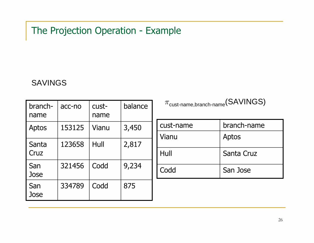
The Projection Operation - Example
875Codd334789San Jose
9,234Codd321456San Jose
2,817Hull123658Santa Cruz
3,450Vianu153125Aptos
balancecust-name
acc-nobranch-name
San JoseCodd
Santa CruzHull
AptosVianu
branch-namecust-name
SAVINGS
πcust-name,branch-name(SAVINGS)

27
More on the Syntax of the Projection Operation
� In relational algebra, attributes can be referenced by position no.
� Projection Operation:
� Syntax: πi1,…,im(R), where R is of arity k, and i_1, ….i_m are
distinct integers from 1 up to k.
� Semantics:
πi1,…,im(R) = {(a1,…,am): there is a tuple (b1,…,bk) in R such that
a1 = bi1, …, am = bim
}
� Example: If R is R(A,B,C,D), then πC,A (R) = π3,1(R)
28
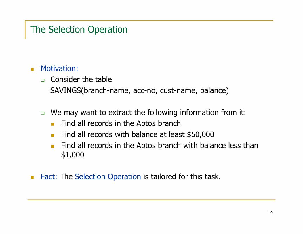
The Selection Operation
� Motivation:
� Consider the table
SAVINGS(branch-name, acc-no, cust-name, balance)
� We may want to extract the following information from it:
� Find all records in the Aptos branch
� Find all records with balance at least $50,000
� Find all records in the Aptos branch with balance less than $1,000
� Fact: The Selection Operation is tailored for this task.

29
The Selection Operation
� Selection is a family of unary operations of the form
σΘ (R),
where R is a relation and Θ is a condition that can be applied as a
test to each row of R.
� When a selection operation is applied to R, it returns the subset of R consisting of all rows that satisfy the condition Θ
� Question: What is the precise definition of a “condition”?

30
The Selection Operation
� Definition: A condition in the selection operation is an expression built up from:
� Comparison operators =, <, >, ≠, ≤, ≥ applied to operands that are constants or attribute names or component numbers.
� These are the basic (atomic) clauses of the conditions.
� The Boolean logic operators Æ, Ç, ¬ applied to basic clauses.
� Examples:
� balance > 10,000
� branch-name = “Aptos”
� (branch-name = “Aptos”) Æ (balance < 1,000)

31
The Selection Operator
� Note:
� The use of the comparison operators <, >, ≤, ≥ assumes that the underlying domain of values is totally ordered.
� If the domain is not totally ordered, then only = and ≠ are allowed.
� If we do not have attribute names (hence, we can only reference columns via their component number), then we need to have a special symbol, say $, in front of a component number. Thus,
� $4 > 100 is a meaningful basic clause
� $1 = “Aptos” is a meaningful basic clause, and so on.
32
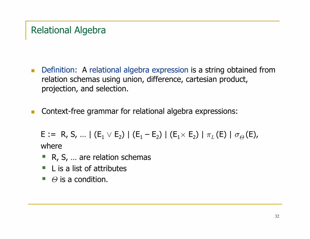
Relational Algebra
� Definition: A relational algebra expression is a string obtained from relation schemas using union, difference, cartesian product, projection, and selection.
� Context-free grammar for relational algebra expressions:
E := R, S, … | (E1 Ç E2) | (E1 – E2) | (E1× E2) | πL (E) | σΘ (E),
where
� R, S, … are relation schemas
� L is a list of attributes
� Θ is a condition.

33
Strength from Unity and Combination
� By itself, each basic relational algebra operation has limited expressive power, as it carries out a specific and rather simple task.
� When used in combination, however, the five relational algebra operations can express interesting and, quite often, rather complex queries.
� Derived relational algebra operations are operations on relations that are expressible via a relational algebra expression (built from the five basic operators).

34
Intersection
� Intersection
� Input: Two k-ary relations R and S, for some k.
� Output: The k-ary relation R S, where
R S = {(a1,…,ak): (a1,…,ak) is in R and (a1,…,ak) is in S}
� Fact: R S = R – (R – S) = S – (S – R)
Thus, intersection is a derived relational algebra operation.

35
Natural Join
� Fact: The most FAQs against databases involve the
natural join operation ⋈.
� Motivating Example: Given
TEACHES(fac-name,course,term) and
ENROLLS(stud-name,course,term),
we want to obtain
TAUGHT-BY(stud-name,course,term,fac-name)
It turns out that TAUGHT-BY = ENROLSS ⋈ TEACHES

36
Natural Join
Given TEACHES(fac-name,course,term) and
ENROLLS(stud-name, course,term):
To compute TAUGHT-BY(stud-name,course,term,fac-name)
1. ENROLLS × TEACHES
2. σ T.course = E.course Æ T.term = E.term (ENROLLS × TEACHES)
3. π stud-name,E.course,E.term,fac-name
(σ T.course = E.course Æ T.term = E.term (ENROLLS × TEACHES))
The result is ENROLLS ⋈ TEACHES.

37
Natural Join
� Definition: Let A1, …, Ak be the common attributes of two relation schemas R and S. Then
R ⋈ S = π<list> (σ R.A1=S.A1 Æ … Æ R.A1 = S.Ak (R×S)),
where <list> contains all attributes of R×S, except for
S.A1, …, S.Ak (in other words, duplicate columns are eliminated).
� Algorithm for R ⋈ S:
For every tuple in R, compare it with every tuple in S as follows:
� test if they agree on all common attributes of R and S;
� if they do, take the tuple in R × S formed by these two tuples,
� remove all values of attributes of S that also occur in R;
� put the resulting tuple in R ⋈ S.
38
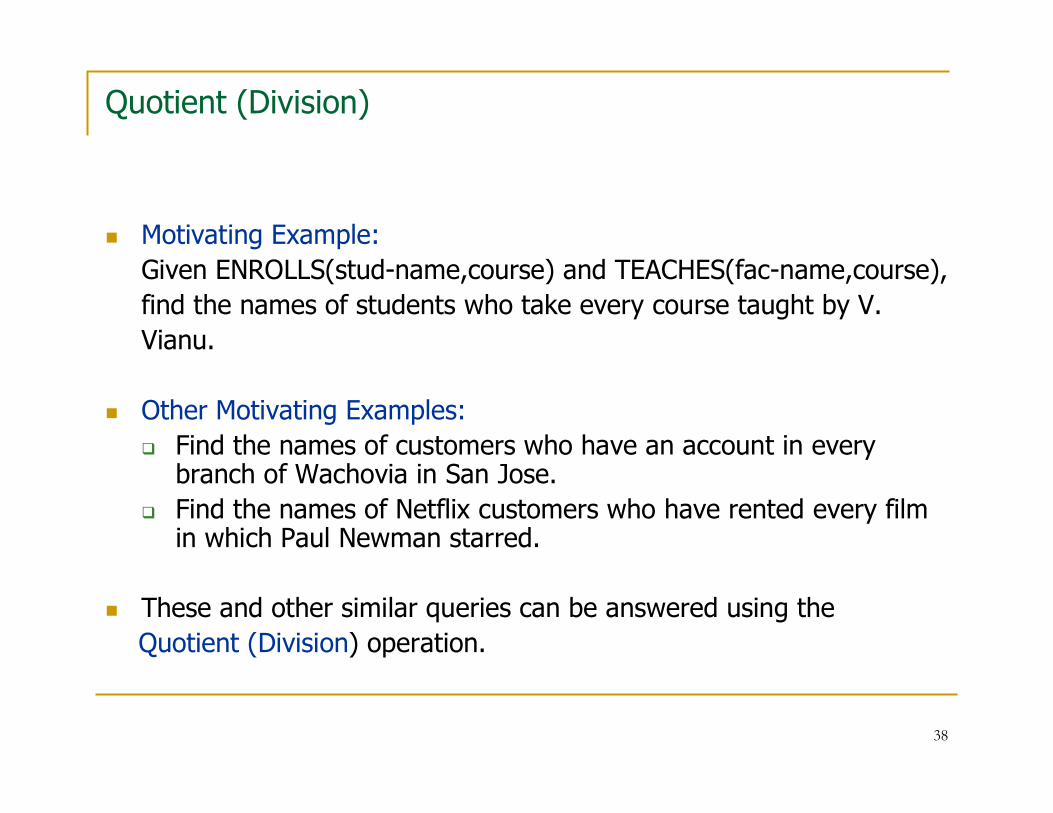
Quotient (Division)
� Motivating Example:
Given ENROLLS(stud-name,course) and TEACHES(fac-name,course),
find the names of students who take every course taught by V.
Vianu.
� Other Motivating Examples:
� Find the names of customers who have an account in every branch of Wachovia in San Jose.
� Find the names of Netflix customers who have rented every film in which Paul Newman starred.
� These and other similar queries can be answered using the
Quotient (Division) operation.

39
Quotient (Division)
� Definition: Let R be a relation of arity r and let S be a relation of arity s, where r > s.
The quotient (or division) R ÷ S is the relation of arity r – s consisting of all tuples (a1,…,ar-s) such that for every tuple (b1,…,bs) in S, we have that (a1,…,ar-s, b1,…,bs) is in R.
� Example: Given
ENROLLS(stud-name,course) and TEACHES(fac-name,course), find the names of students who take every course taught by V. Vianu.
� Find the courses taught by V. Vianu
πcourse (σ fac-name = “V. Vianu” (TEACHES))
� The desired answer is given by the expression:
ENROLLS ÷ πcourse (σ fac-name = “V. Vianu” (TEACHES))
40
Quotient (Division)
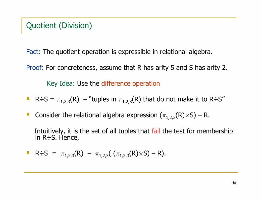
Fact: The quotient operation is expressible in relational algebra.
Proof: For concreteness, assume that R has arity 5 and S has arity 2.
Key Idea: Use the difference operation
� R÷S = π1,2,3(R) – “tuples in π1,2,3(R) that do not make it to R÷S”
� Consider the relational algebra expression (π1,2,3(R)×S) – R.
Intuitively, it is the set of all tuples that fail the test for membership in R÷S. Hence,
� R÷S = π1,2,3(R) – π1,2,3( (π1,2,3(R)×S) – R).

41
The Expressive Power of Relational Algebra
� When combined together, the five basic relational algebra operations can express interesting and complex queries.
� In particular, relational algebra can express:
� The Intersection Operation
� The Natural Join Operation
� The Quotient Operation
� ….
42
Independence of the Basic Relational Algebra Operations
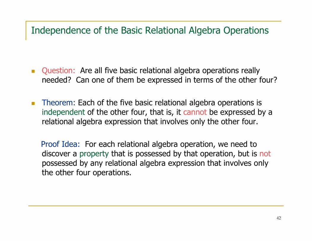
� Question: Are all five basic relational algebra operations really needed? Can one of them be expressed in terms of the other four?
� Theorem: Each of the five basic relational algebra operations is independent of the other four, that is, it cannot be expressed by a relational algebra expression that involves only the other four.
Proof Idea: For each relational algebra operation, we need to discover a property that is possessed by that operation, but is not possessed by any relational algebra expression that involves only the other four operations.

43
Independence of the Basic Relational Algebra Operations
Theorem: Each of the five basic relational algebra operations is independent of the other four, that is, it cannot be expressed by a relational algebra expression that involves only the other four.
Proof Sketch: (projection and cartesian product only)� Property of projection:
� It is the only operation whose output may have arity smaller than its input.� Show, by induction, that the output of every relational algebra expression
in the other four basic relational algebra is of arity at least as big as the maximum arity of its arguments.
� Property of cartesian product: � It is the only operation whose output has arity bigger than its input.� Show, by induction, that the output of every relational algebra expression
in the other four basic relational algebra is of arity at most as big as the maximum arity of its arguments.
Exercise: Complete this proof.

44
Relational Algebra: Summary
� When combined with each other, the five basic relational algebraoperations can express interesting and complex queries (natural join, quotient, …)
� The five basic relational algebra operations are independent of each other: none can be expressed in terms of the other four.
� So, in conclusion, Codd’s choice of the five basic relational algebra operations has been very judicious.

45
Relational Completeness
� Definition (Codd – 1972): A database query language L is relationally complete if it is at least as expressive as relational algebra, i.e., every relational algebra expression E has an equivalent expression F in L.
� Relational completeness provides a benchmark for the expressive power of a database query language.
� Every commercial database query language should be at least as expressive as relational algebra.
� Exercise: Explain why SQL is relationally complete.

46
SQL vs. Relational Algebra
Selection σWHERE
Cartesian Product ×FROM
Projection πSELECT
Relational AlgebraSQL
Semantics of SQL via interpretation to Relational Algebra
SELECT Ri1.A1, …, Rim.A.m
FROM R1, …,RK = π Ri1.A1, …, Rim.A.m (σΨ (R1 × … × RK))
WHERE Ψ

47
Relational Calculus
� In addition to relational algebra, Codd introduced relational calculus.
� Relational calculus is a declarative database query language based on first-order logic.
� Relational calculus comes into two different flavors:
� Tuple relational calculus
� Domain relational calculus.
We will focus on domain relational calculus.
There is an easy translation between these two formalisms.
� Codd’s main technical result is that relational algebra and relationalcalculus have essentially the same expressive power.

48
Propositional Logic (aka Boolean Logic) Reminder
� Propositional variables: x, y, z, …
� They take values 0 (True) and 1 (False).
� Propositional connectives: Æ, Ç, ¬, →
� Propositional formulas: expressions built from propositional variables and propositional connectives
� Syntax: ϕ := x, y, z, … | (ψ Æ χ) | (ψ Ç χ) | ¬ ψ | (ψ → χ)
� Semantics: Truth-table semantics
� Application: Propositional formulas express Boolean functions
� (x Ç y) Æ (¬ x Ç ¬ y) XOR-Gate
� (x Æ y) Ç (x Æ z) Ç (y Æ z) Majority Gate

49
First-Order Logic - Motivation
� First-Order Logic is a formalism for expressing properties of mathematical structures (graphs, trees, partial orders, …).
� Example: Consider a graph G=(V,E) (nodes are in V, edges are in E)
� There is a self-loop.
� Every two nodes are connected via a path of length 2.
� Every node has exactly three distinct neighbors.
� There is a path of length 3 from node x to node y.
� Node x has at least four distinct neighbors
These and many other similar properties are expressible as
formulas of first-order logic on graphs.
� One of Codd’s key insights was that first-order logic can also be used to express relational database queries.
50
First-Order Logic
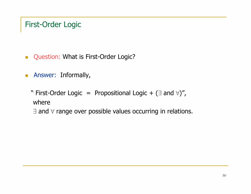
� Question: What is First-Order Logic?
� Answer: Informally,
“ First-Order Logic = Propositional Logic + (∃ and ∀)”,
where
∃ and ∀ range over possible values occurring in relations.

51
Relational Calculus (First-Order Logic for Databases)
� First-order variables: x, y, z, …, x1, …,xk,…
� They range over values that may occur in tables.
� Relation symbols: R, S, T, … of specified arities (names of relations)
� Atomic (Basic) Formulas:
� R(x1,…,xk), where R is a k-ary relation symbol
(alternatively, (x1,…,xk) ∈ R; the variables need not be distinct)
� (x op y), where op is one of =, ≠, <, >, ≤, ≥
� (x op c), where c is a constant and op is one of =, ≠, <, >, ≤, ≥.
� Relational Calculus Formulas:
� Every atomic formula is a relational calculus formula.
� If ϕ and ψ are relational calculus formulas, then so are:
� (ϕ Æ ψ), (ϕ Ç ψ), ¬ ψ, (ϕ → ψ) (propositional connectives)
� (∃ x ϕ) (existential quantification)
� (∀ x ϕ) (universal quantification).

52
Relational Calculus
� Examples: Assume E is a binary relation symbol
� (∃ x)E(x,x)
� (∀ x)(∀ y)(∃ z)(E(x,z) Æ E(z,y))
� (∃ z1)(∃ z2)(E(x,z1) Æ E(z1,z2) Æ E(z2,y))
� (∃ y)(∃ z)(E(x,y) Æ E(x,z) Æ (y≠z))
� Free and bound variables:
� In the first two formulas above, no variable is free.
� In the third formula above, the free variables are x and y.
� In the fourth formula above, the only free variable is x.
� Intuitively, a variable is free in a formula if the variable must be assigned a value in order to tell if the formula is true or false.

53
Relational Calculus as a Database Query Language
Definition:
� A relational calculus expression is an expression of the form
{(x1,…,xk): ϕ(x1,…xk)},
where ϕ(x1,…,xk) is a relational calculus formula with x1,…,xk as its free variables.
� When applied to a relational database I, this relational calculus expression returns the k-ary relation that consists of all k-tuples(a1,…,ak) that make the formula “true” on I.
Example: The relational calculus expression
{(x,y): ∃z(E(x,z) Æ E(z,y))}
returns the set P of all pairs of nodes (a,b) that are connected via a
path of length 2.

54
Relational Calculus as a Database Query Language
Example: FACULTY(name, dpt, salary), CHAIR(dpt, name)
Give a relational calculus expression for C-SALARY(dpt,salary)
(find the salaries of department chairs).
{(x,y): ∃u(FACULTY(u,x,y) Æ CHAIR(x,u))}
Here is another relational calculus expression for the same task:
{(x,y): ∃u∃v(FACULTY(u,x,y) Æ CHAIR(x,v) Æ (u=v))}

55
Relational Calculus as a Database Query Language
Example: FACULTY(name, dpt, salary)
Find the names of the highest paid faculty in CS
{x: ϕ(x)}, where ϕ(x) is the formula:
∃y,z (FACULTY(x,y,z) Æ y = “CS” Æ
(∀u,v,w(FACULTY(u,v,w) Æ v = “CS” → z ≥ w)))
Exercise: Express this query in relational algebra and in SQL.
Abbreviation:
� ∃x1,…,xk stands for ∃x1,…,∃xk
� ∀x1,…,xk stands for ∀x1,…,∀xk

56
Natural Join in Relational Calculus
Example: Let R(A,B,C) and S(B,C,D) be two ternary relation schemas.
� Recall that, in relational algebra, the natural join R ⋈ S is given by
π R.A,R.B,R.C,S.D (σ R.B = S.B Æ R.C = S.C (R × S)).
� Give a relational calculus expression for R ⋈ S
{(x1,x2,x3,x4): R(x1,x2,x3) Æ S(x2,x3,x4)}
Note: The natural join is expressible by a quantifier-free formula of
relational calculus.
57
Quotient in Relational Calculus
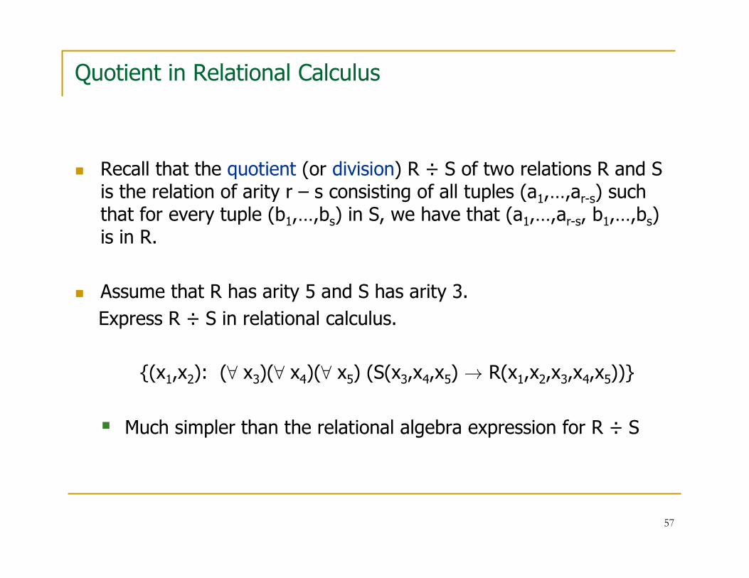
� Recall that the quotient (or division) R ÷ S of two relations R and S is the relation of arity r – s consisting of all tuples (a1,…,ar-s) such that for every tuple (b1,…,bs) in S, we have that (a1,…,ar-s, b1,…,bs) is in R.
� Assume that R has arity 5 and S has arity 3.
Express R ÷ S in relational calculus.
{(x1,x2): (∀ x3)(∀ x4)(∀ x5) (S(x3,x4,x5) → R(x1,x2,x3,x4,x5))}
� Much simpler than the relational algebra expression for R ÷ S

58
Relational Algebra vs. Relational Calculus
Codd’s Theorem (informal statement):
Relational Algebra and Relational Calculus have essentially the same
expressive power, i.e., they can express the same queries.
Note:
� This statement is not entirely accurate.
� In what follows, we will give a rigorous formulation of Codd’sTheorem and sketch its proof.

59
Queries
Definition: Let S be a relational database schema.
A k-ary query on S is a function q defined on database instances over S
such that if I is a database instance over S, then q(I) is a k-ary relation
that is invariant under isomorphisms and has values among those
occurring in the relations in I
(i.e., if h: I → J is an isomorphism, then q(J) = h(q(I)).
Note:
� All “queries” that we have expressed in relational algebra and/or in relational calculus so far are queries in the above formal sense.
� In particular, a relational calculus expression of the form
{(x1,…,xk): ϕ(x1,…xk)} defines a k-ary query.

60
From Relational Algebra to Relational Calculus
Theorem: For every relational expression E, there is an equivalent relational calculus expression {(x1,…,xk): ϕ(x1,…xk)}.
Proof: By induction on the construction of rel. algebra expressions.
� If E is a relation R of arity k, then we take {(x1,…,xk): E(x1,…,xk)}.
� Assume E1 and E2 are expressible by {(x1,…,xk): ϕ1(x1,…,xk)} and by{(x1,…,xm): ϕ2(x1,…,xm)}. Then� E1 ∪ E2 is expressible by
{(x1,…,xk): ϕ1(x1,…,xk) Ç ϕ2(x1,…,xk)}.
� E1 – E2 is expressible by{(x1,…,xk): ϕ1(x1,…,xk) Æ ¬ϕ2(x1,…,xk)}.
� E1 × E2 is expressible by{(x1,…,xk,y1,…,ym): ϕ1 (x1,…,xk) Æ ϕ2(y1,…,ym)}

61
From Relational Algebra to Relational Calculus
Theorem: For every relational expression E, there is an equivalent relational calculus expression {(x1,…,xk): ϕ(x1,…xk)}.
Proof: (continued)� Assume that E is expressible by {(x1,…,xk): ϕ(x1,…,xk)}.
Then� π1,3(E) is expressible by
{(x1,x3): (∃ x2)(∃ x4) …(∃ xk) ϕ(x1,…,xk) }� σΘ(E) is expressible by
{(x1,…,xk): Θ* Æ ϕ(x1,…,xk)}, where Θ* is the rewriting of Θ as a formula of relational calculus.
Corollary: Relational Calculus is relationally complete.

62
From Relational Calculus to Relational Algebra
Fact: It is not true that for every relational calculus expression ϕ,
there is an equivalent relational algebra expression E.
Examples:
� {(x1,…,xk): ¬ R(x1,…,xk)}
� {(x,y): ∃z(CHAIR(x,z) Æ y≠z)}, where CHAIR(dpt,name)
� {x: ∀y,z ENROLLS(x,y,z)}, where ENROLLS(s-name,course,term)

63
From Relational Calculus to Relational Algebra
Note: The previous three relational calculus expression produce
different answers when we consider different domains over which
the variables are interpreted.
Example: If the variables x1,…,xk range over a domain D, then
{(x1,…,xk): ¬ R(x1,…,xk)} = Dk – R.
Fact:
� The relational calculus expression {(x1,…,xk): ¬ R(x1,…,xk)}
is not “domain independent”.
� The relational calculus expression
{(x1,…,xk): S(x1,..,xk) Æ ¬ R(x1,…,xk)} is “domain independent”.

64
From Relational Calculus to Relational Algebra
� Question: How can we go from relational calculus to relational algebra?
� Answer: There are two possibilities:
� Restrict ourselves to “domain independent” relational calculus expressions.
� “Relativize” the semantics of relational calculus expressions by fixing a domain over which the variables range.

65
Active Domain
Definition:
� The active domain adom(ϕ) of a relational calculus formula ϕ is the set of all constants that occur in ϕ.
� If ϕ is R(x,y), then adom(ϕ) = ∅
� If ϕ is ∃y(R(x,y) Æ (y > 3) Æ (x < 5)), then adom(ϕ) = {3,5}.
� The active domain adom(I) of a relational database instance I is the set of all values that occur in the relations of I.

66
Active Domain and Relative Interpretations
Definition: Let ϕ(x1,…,xk) be a relational calculus formula and let I be a
relational database instance.
� If is D a domain such adom(ϕ) ∪ adom(I) ⊆ D, then
ϕD(I) is the result of evaluating ϕ(x1,…,xk) over D and I, that is,
� all variables and quantifiers are assumed to range over D;
� the relation symbols in ϕ are interpreted by the relations in I.
� By definition, ϕadom(I) is ϕD(I), where D = adom(ϕ) ∪ adom(I).

67
Active Domain and Relative Interpretation
Example: Let ϕ be ¬R(x,y) and I = {(1,2)}.
� adom(I) = {1,2}
� ϕadom (I) = {(2,1), (1,1), (2,2)}
� If D = {1,2,3}, then
ϕD(I)= {(2,1),(1,1),(2,2),(3,3),(1,3),(3,1),(2,3),(3,2)}

68
Active Domain and Relative Interpretation
Example: Let ϕ be ∃yR(x,y) and I = {(1,1),(1,2),(2,1),(1,3)}.
� adom(I) = {1,2,3}
� ϕadom (I) = {1,2}
� If D = {1,2,3,4}, then
ϕD(I) = {1,2}.
� More generally, if adom(I) ⊆ D, then
ϕD(I) = {1,2}.

69
Active Domain and Relative Interpretation
Example: Let ϕ be ∀yR(x,y) and I = {(1,1),(1,2),(2,1)}.
� adom(I) = {1,2}
� ϕadom (I) = {1}
� If D = {1,2,3}, then
ϕD(I)= ∅.

70
Domain Independence
Definition: A relational calculus formula ϕ is domain independent
if for every relational instance I and every domain D such that
adom(ϕ) ∪ adom(I) ⊆ D, we have that
ϕD(I) = ϕadom(I).
Examples:
� ¬R(x1,…,xk) is not domain independent.
� ∃yR(x,y) is domain independent.
� ∀yR(x,y) is not domain independent.
� ∀y(R(x,y) → y > 5) is domain independent.
71
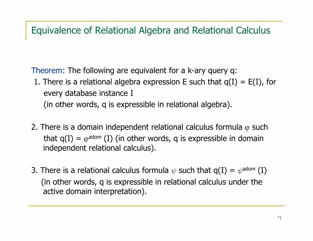
Equivalence of Relational Algebra and Relational Calculus
Theorem: The following are equivalent for a k-ary query q:
1. There is a relational algebra expression E such that q(I) = E(I), for
every database instance I
(in other words, q is expressible in relational algebra).
2. There is a domain independent relational calculus formula ϕ such
that q(I) = ϕadom (I) (in other words, q is expressible in domain independent relational calculus).
3. There is a relational calculus formula ψ such that q(I) = ψadom (I)
(in other words, q is expressible in relational calculus under the active domain interpretation).
72
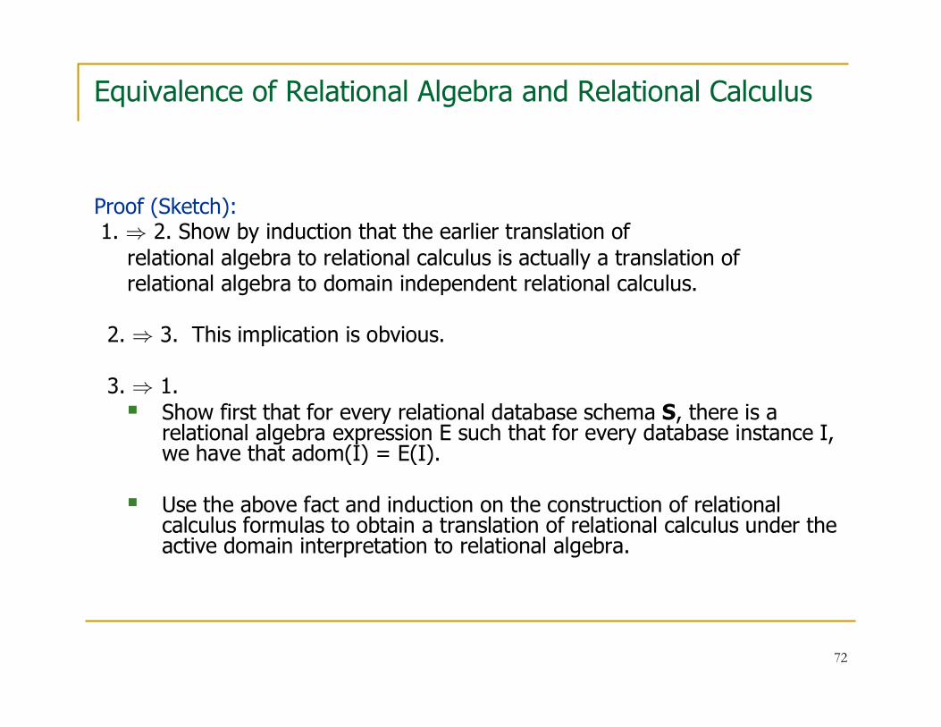
Equivalence of Relational Algebra and Relational Calculus
Proof (Sketch):1. ⇒ 2. Show by induction that the earlier translation of
relational algebra to relational calculus is actually a translation of relational algebra to domain independent relational calculus.
2. ⇒ 3. This implication is obvious.
3. ⇒ 1. � Show first that for every relational database schema S, there is a
relational algebra expression E such that for every database instance I, we have that adom(I) = E(I).
� Use the above fact and induction on the construction of relational calculus formulas to obtain a translation of relational calculus under the active domain interpretation to relational algebra.

73
Equivalence of Relational Algebra and Relational Calculus
� In this translation, the most interesting part is the simulation of the universal quantifier ∀ in relational algebra.
� It uses the logical equivalence ∀yψ ≡ ¬∃y¬ψ
� As an illustration, consider ∀yR(x,y).
� ∀yR(x,y) ≡ ¬∃y¬R(x,y)
� adom(I) = π(R) ∪ π(R)
(π(R) ∪ π(R)) – (π((π(R) ∪ π(R))×(π(R) ∪ π(R)) - R))¬∃y¬R(x,y)
π((π(R) ∪ π(R))×(π(R) ∪ π(R)) - R)∃y¬R(x,y)
(π(R) ∪ π(R))×(π(R) ∪ π(R)) – R¬ R(x,y)
Relational Algebra Expression for ϕadomRel.Calc. formula ϕ

74
Equivalence of Relational Algebra and Relational Calculus
Remarks:
� The Equivalence Theorem is effective. Specifically, the proof of this theorem yields two algorithms:
� an algorithm for translating from relational algebra to domain independent relational calculus, and
� an algorithm from translating from domain independent relationalcalculus to relational algebra.
� Each of these two algorithms runs in linear time.

75
Domain Independent Relational Calculus
Note:
� A desirable feature of a logical formalism is that there is an (efficient) algorithm for determining whether or not an expression is a formula of that formalism.
� Both relational algebra and relational calculus have this property.
Question:
� Does domain independent relational calculus have this property?
� In other words, is there an algorithm such that, given a relational calculus formula ϕ, the algorithm tells whether or not ϕ is domain independent?

76
Domain Independent Relational Calculus
Bad News …
Theorem (Di Paola – 1969): Determining domain independence is an
undecidable problem, i.e., there is no algorithm such that, given a
relational calculus formula ϕ, the algorithm tells whether or not ϕ is
domain independent.
Some Good News:
Theorem: Domain independent relational calculus has an effective
syntax, i.e., there is a class F of relational calculus formulas such that:
� There is an (efficient) algorithm for testing membership in F.
� Every formula in F is domain independent.
� Every domain independent relational calculus formula is logically equivalent to a formula in F.

77
Domain Independent Relational Calculus
For much more on domain independence:
� Read Sections 5.3 and 5.4 of “Foundations of Databases” by Abiteboul, Hull, and Vianu
� Read the papers
� “The recursive unsolvability of the decision problem for the class of definite formulas” by Robert A. Di Paola, JACM, Vol. 16, 1969, pages 324-327.
� “Safety and translation of relational calculus” by Allen van Gelderand Rodney Topor, ACM Transactions on Database Systems, Vol. 16, 1991, pages 235 – 278.
78
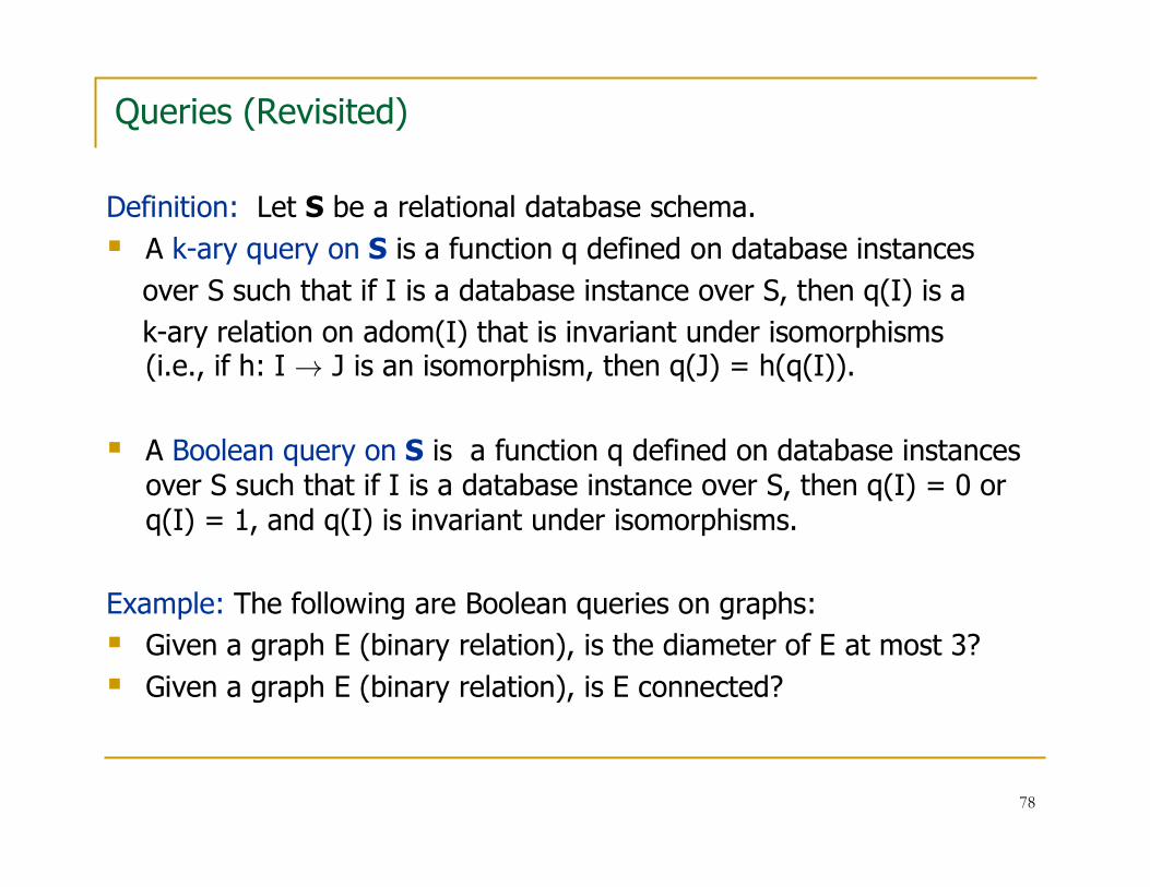
Queries (Revisited)
Definition: Let S be a relational database schema.
� A k-ary query on S is a function q defined on database instances
over S such that if I is a database instance over S, then q(I) is a
k-ary relation on adom(I) that is invariant under isomorphisms(i.e., if h: I → J is an isomorphism, then q(J) = h(q(I)).
� A Boolean query on S is a function q defined on database instances over S such that if I is a database instance over S, then q(I) = 0 or q(I) = 1, and q(I) is invariant under isomorphisms.
Example: The following are Boolean queries on graphs:
� Given a graph E (binary relation), is the diameter of E at most 3?
� Given a graph E (binary relation), is E connected?

79
Three Fundamental Algorithmic Problems about Queries
� The Query Evaluation Problem: Given a query q and a database instance I, find q(I).
� The Query Equivalence Problem: Given two queries q and q’ of the same arity, is it the case that q ≡ q’ ?
(i.e., is it the case that, for every database instance I, we have that q(I) = q’(I)?)
� The Query Containment Problem: Given two queries q and q’ of the same arity, is it the case that q ⊆ q’ ?
(i.e., is it the case that, for every database instance I, we have that q(I) ⊆ q’(I)?)

80
Three Fundamental Algorithmic Problems about Queries
� The Query Evaluation Problem is the main problem in query processing.
� The Query Equivalence Problem underlies query processing and optimization, as we often need to transform a given query to an equivalent one.
� The Query Containment Problem and Query Equivalence Problemare closely related to each other:
� q ≡ q’ if and only if q ⊆ q’ and q’ ⊆ q.
� q ⊆ q’ if and only if q ≡ q Æ q’.

81
Three Fundamental Algorithmic Problems about Queries
� Our goal is to investigate the algorithmic aspects of these problems for queries expressible in relational algebra/relational calculus.
� The questions we want to address are:
� How can we measure the precise “difficulty” of these problems?
� Are there “good” algorithms for solving these problems?
� If not, are there special cases of these problems for which “good”algorithms exist?

82
Three Fundamental Algorithmic Problems about Queries
Our study of these problems will use concepts and methods from two
different, yet related, areas:
� Mathematical Logic:
� Computability Theory and Undecidable Problems
� Computational Complexity Theory:
� Complexity Classes and Complete Problems
� In particular, the classes P and NP, and NP-complete problems.

83
Decision Problems and Languages
� Definition (informal): A decision problem Q consists of a set of inputs and a question with a “yes” or “no” answer for each input.
� Definition:
� Σ* is the set of all strings over a finite alphabet Σ.
� A language over Σ is a set L ⊆ Σ*
� Every language L gives rise to the following decision problem:
� Given x ∈ Σ*, is x ∈ L?
� Conversely, every decision problem can be thought of as arising
from a language, namely,
the language consisting of all inputs with a “yes” answer.
Q?input x
1 (“yes”)
0 (“no”)
84
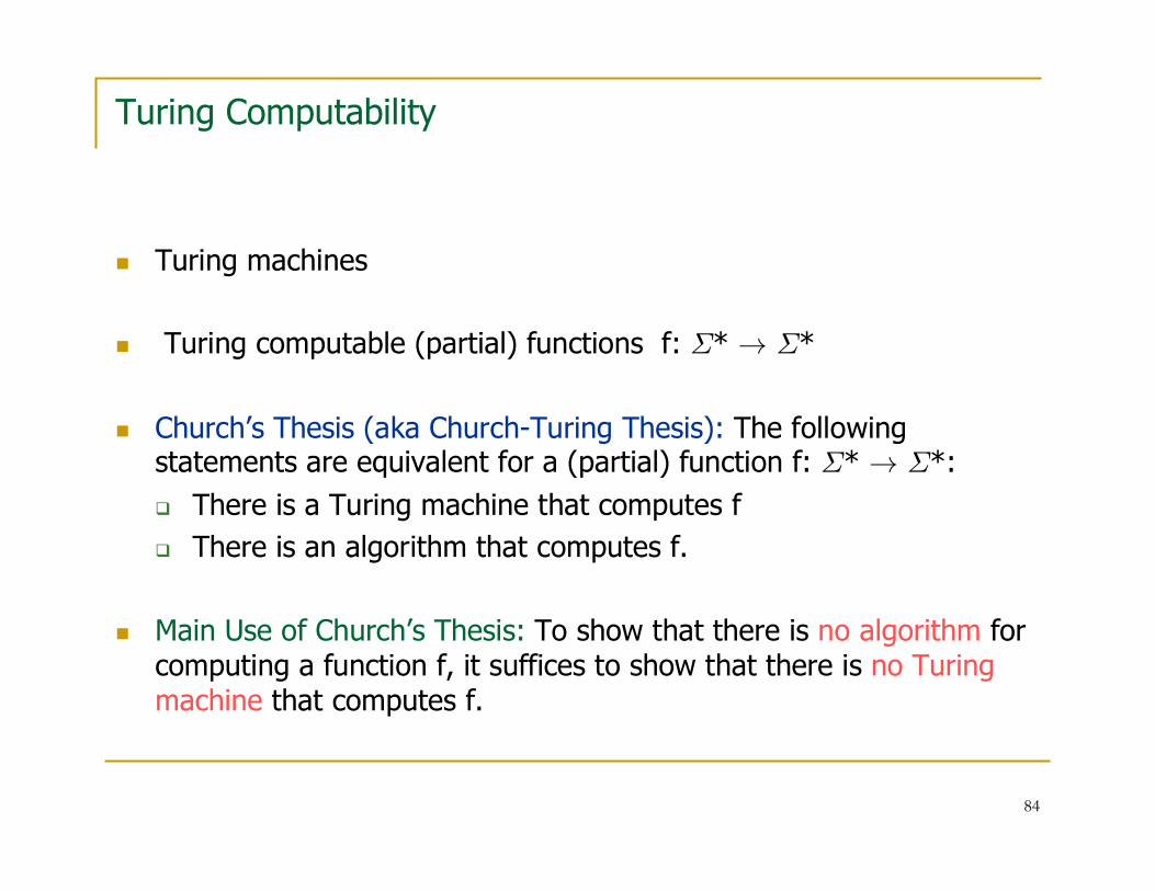
Turing Computability
� Turing machines
� Turing computable (partial) functions f: Σ* → Σ*
� Church’s Thesis (aka Church-Turing Thesis): The following statements are equivalent for a (partial) function f: Σ* → Σ*:
� There is a Turing machine that computes f
� There is an algorithm that computes f.
� Main Use of Church’s Thesis: To show that there is no algorithm for computing a function f, it suffices to show that there is no Turing machine that computes f.

85
Recursive and Recursively Enumerable Languages
� Definition: Let L ⊆ Σ* be a language
� L is recursive if its characteristic function χ is Turing computable, where
� χL(x) = 1 if x ∈ L
� χL(x) = 0 if x ∉ L.
� L is recursively enumerable if its semi-characteristic function sL is Turing computable, where
� sL(x) = 1 if x ∈ L
� sL(x) = undefined if x ∉ L.
� Theorem: The following are equivalent for a language L ⊆ Σ* :
� L is recursive.
� Both L and its complement Σ* - L are recursively enumerable.

86
Decidable and Undecidable Problems
� Definition: Let Q be a decision problem.
� Q is decidable (solvable) if the language associated with Q is recursive.
� Q is undecidable (unsolvable) if the language associated with Q is not recursive.
Q? Input x
1 (yes)
0 (“no”)
Q is undecidable means that there is no algorithm for this problem

87
Undecidable Problems
Fact: Undecidable problems exist.
Proof: Use a counting argument:
� There are countably many Turing machines.
� There are uncountably many languages L ⊆ {0,1}*.
Theorem: Many natural problems of algorithmic interest or of
mathematical significance are undecidable.

88
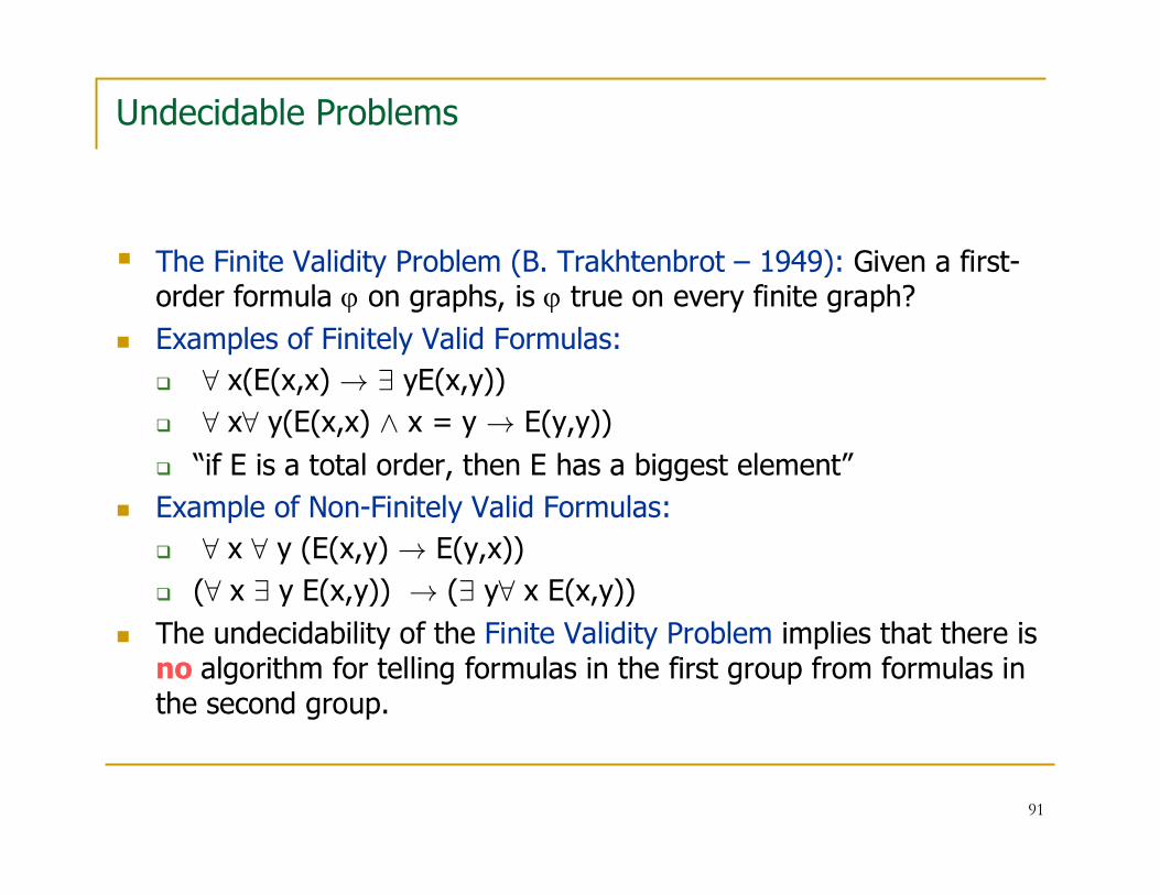
Undecidable Problems
Theorem: The following problems are undecidable:
� The Halting Problem (A. Turing – 1936): Given a Turing machine M and an input x, does M halt on x?
� The Finite Validity Problem (B. Trakhtenbrot – 1949): Given a first-order formula ϕ on graphs, is ϕ true on every finite graph?
� Hilbert’s 10th Problem (Y. Matijacevic – 1971): Given a multivariate polynomial p(x1,…,xn) with integer coefficients, does p(x1,…,xn) have an all-integers solution?

89
Undecidable Problems
� The Halting Problem (A. Turing – 1936): Given a Turing machine M and an input x, does M halt on x?
� Implications of Undecidability of the Halting Problem:
� The undecidability of the Halting Problem implies that there is noalgorithm such that, given a C program p and an input x, the algorithm determines whether the program p produces an output on input x or goes into an infinite loop.
� Of course, it may still be possible to show that a particular program terminates on a given input (or even on every input), but it is not possible to automate this process for every program.
� But even this may be a difficult task …

90
Proving Program Termination
� McCarthy’s Program
Given a positive integer n:
While n > 1, do:
� If n is even, then set n: = n/2;
� If n is odd, then set n:= 3n+1.
� Example Run:
� n = 11 ֏ 34 ֏ 17 ֏ 52 ֏ 26 ֏ 13 ֏ 40 ֏ 20 ֏ 10
֏ 5 ֏ 16 ֏ 8 ֏ 4 ֏ 2 ֏ 1.
� Open Problem: Does this program terminate on every input?
91
Undecidable Problems
� The Finite Validity Problem (B. Trakhtenbrot – 1949): Given a first-order formula ϕ on graphs, is ϕ true on every finite graph?
� Examples of Finitely Valid Formulas:
� ∀ x(E(x,x) → ∃ yE(x,y))
� ∀ x∀ y(E(x,x) Æ x = y → E(y,y))
� “if E is a total order, then E has a biggest element”
� Example of Non-Finitely Valid Formulas:
� ∀ x ∀ y (E(x,y) → E(y,x))
� (∀ x ∃ y E(x,y)) → (∃ y∀ x E(x,y))
� The undecidability of the Finite Validity Problem implies that there is no algorithm for telling formulas in the first group from formulas in the second group.

92
Undecidable Problems
� Hilbert’s 10th Problem (Y. Matijacevic – 1971): Given a multivariate polynomial p(x1,…,xn) with integer coefficients, does p(x1,…,xn) have an all-integers root ? (i.e., does the equation p(x1,…,xn) = 0 have an all integer solution?)
� Diophantine Equations (Diophantus of Alexandria 3rd Century AD)
� 3x + 5y - 8z = 0
� x2 – 2xy + z3 + 9 = 0
� x2 – 100y2
+ 1 = 0
� x2 + y2 - z2 = 0
� x3 + y3 - z3 = 0
� The undecidability of Hilbert’s 10th Problem implies that there is noalgorithm to tell whether or not a given Diophantine equation has a solution consisting entirely of integers.

93
Undecidable Problems
Note:
� The Halting Problem is recursively enumerable, but not recursive
(hence, its complement is not recursively enumerable).
� The Finite Validity Problem is co-recursively enumerable, but not recursive.
(hence, it is not even recursively enumerable).
� Hilbert’s 10th Problem is recursively enumerable, but not recursive
(hence, its complement is not recursively enumerable).

94
The Reduction Method
� By now there is a vast library of undecidable problems.
� The Reduction Method is the main technique for establishing undecidability.
� Reduction Method: To show that a language L* is not recursive, it suffices to find a non-recursive language L and a total Turing computable function f such that for every string x, we have that
x ∈ L ⇔ f(x) ∈ L*.
� Such a function f is called a reduction of L to L*
� L ≼ L* means that there is a reduction of L to L*.

95
The Reduction Method
� The Halting Problem was the first fundamental decision problem shown to be undecidable.
� The Finite Validity Problem was shown to be undecidable by showing that Halting Problem ≼ Finite Validity Problem.
� Many database problems have been shown to be undecidable via reductions from one the following problems:
� The Halting Problem
� The Finite Validity Problem
� Hilbert’s 10th Problem.
� In particular, Di Paola proved that the Domain Independence Problem for relational calculus formulas is undecidable by showing that Finite Validity Problem ≼ Domain Independence.

96
Undecidability of The Query Equivalence Problem
� The Query Equivalence Problem: Given two queries q and q’ of the same arity, is it the case that q ≡ q’ ?
(i.e., is q(I) = q’(I) on every database instance I?)
� Theorem: The Query Equivalence Problem for relational calculus queries is undecidable.
Proof: Finite Validity Problem ≼ Query Equivalence Problem
� To see, this let ψ* be a fixed finitely valid relational calculus sentence (say, ∀ x(E(x,x) → ∃ yE(x,y))).
� Then, for every relational calculus sentence ϕ, we have that
ϕ is finitely valid ⇔ ϕ ≡ ψ*.

97
Undecidability of the Query Containment Problem
� The Query Containment Problem: Given two queries q and q’ of the same arity, is it the case that q ⊆ q’ ?
(i.e., is q(I) ⊆ q’(I) on every database instance I?)
� Corollary: The Query Containment Problem for relational calculus queries in undecidable.
Proof: Query Equivalence ≼ Query Containment, since
q ≡ q’ ⇔ q ⊆ q’ and q’ ⊆ q.
� Notice the chain of reductions:
Halting Problem ≼ Finite Validity ≼ Query Equiv. ≼ Query Cont.

98
The Query Evaluation Problem
� The Query Evaluation Problem: Given a query q and a database instance I, find q(I).
� The Query Evaluation Problem for relational calculus queries is decidable, but, as we will see, it has high computational complexity.
� To understand the precise algorithmic difficulty of the Query Evaluation Problem, we need some basic notions and results from computational complexity.

99
Decidable Problems and Computational Complexity
� Computational Complexity is the quantitative study of decidable problems.
� “From these and other considerations grew our deep conviction that there must be quantitative laws that govern the behavior of information and computing. The results of this research effort were summarized in our first paper on this topic, which also named this new research area, "On the computational complexity of algorithms“.”
J. Hartmanis, Turing Award Lecture, 1993
UndecidableProblems
DecidableProblems

100
Computational Complexity Classes
� Decidable problems are grouped together in computational complexity classes.
� Each computational complexity class consists of all problems that can be solved in a computational model under certain restrictions on the resources used to solve the problem.
� Examples of computational models:
� Turing Machine TM (deterministic Turing machine)
� Non-deterministic Turing machine NTM
� …
� Examples of resources:
� Amount of time needed to solve the problem
� Amount of space (memory) needed to solve the problem.
� …

101
The Five Basic Computational Complexity Classes
� LOGSPACE (or, L): All decision problems solvable by a TM using
extra memory bounded by a logarithmic amount in the input size.
� NLOGSPACE (or, NL): All decision problems solvable by a NTM using
extra memory bounded by a logarithmic amount in the input size.
� P (or, PTIME): All decision problems solvable by a TM in time
bounded by some polynomial in the input size.
� NP: All decision problems solvable by a NTM in time bounded by
some polynomial in the input size.
� PSPACE: All decision problems solvable by a TM using memory bounded by a polynomial in the input size.

102
The Five Basic Computational Complexity Classes
Theorem:
� The following inclusions hold:
LOGSPACE ⊆ NLOGSPACE ⊆ P ⊆ NP ⊆ PSPACE.
� Moreover, it is known that LOGSPACE ⊂ PSPACE.
� No other proper inclusion between these classes is known at present. In particular, it is not known whether P = NP.
Note:
� The question: “is P = NP?” is the central open problem in computational complexity.
� It is one of the Millennium Prize Problems – see http://www.claymath.org/millennium/

103
Complete Problems
� A key property of most complexity classes is that they possess complete problems.
� Intuitively, complete problems are the “hardest” problems in the class in the sense that every other problem can be reduced to it.
� Definition: Let C be a complexity class.
A decision problem Q is C-complete if
� Q is in C.
� If Q’ is in C , then there is a “suitable” total Turing computable function f such that for every string x, we have that
x ∈ Q’ ⇔ f(x) ∈ Q.
� “suitable” means that f can be computed with fewer resources than those used to define C.
� So, f is a reduction of a restricted nature.
104
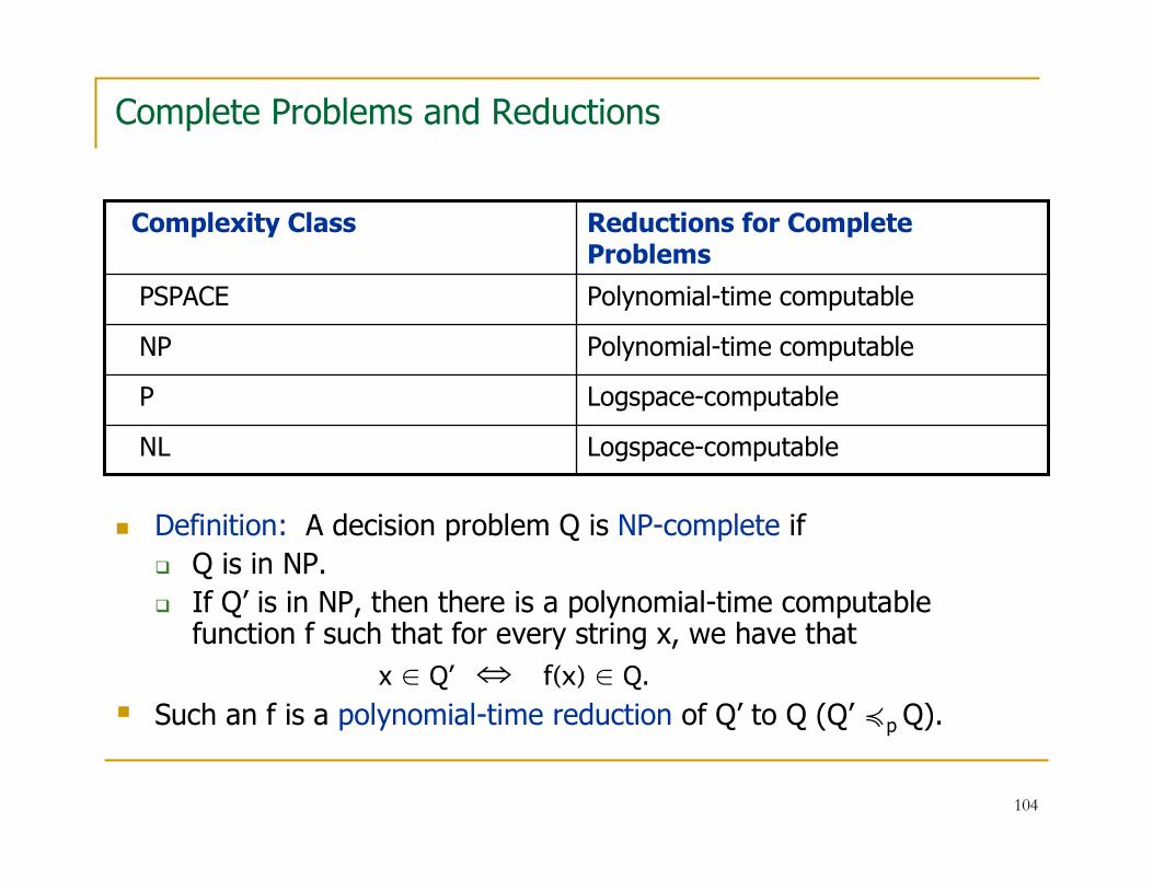
Complete Problems and Reductions
� Definition: A decision problem Q is NP-complete if
� Q is in NP.
� If Q’ is in NP, then there is a polynomial-time computable function f such that for every string x, we have that
x ∈ Q’ ⇔ f(x) ∈ Q.
� Such an f is a polynomial-time reduction of Q’ to Q (Q’ ≼p Q).
Logspace-computableNL
Logspace-computableP
Polynomial-time computableNP
Polynomial-time computablePSPACE
Reductions for Complete Problems
Complexity Class

105
Complete Problems for Computational Complexity Classes
� PSPACE-complete:
� Quantified Boolean Formulas (QBF): Given a quantified Boolean formula ∀ x1∃ x2 …. ∀ xkϕ, is it true?
� NP-complete:
� Satisfiability (SAT): Given a CNF formula ϕ, is it satisfiable?
� 3-Colorability: Given a graph G=(V,E), is it 3-colorable?
� Integer Linear Inequalities (ILI): Given a system of linear inequalities with integer coeffs., does it have an integer solution?
� P-complete:
� Horn SAT: Given a Horn CNF formula ϕ, is it satisfiable?
� Linear Inequalities (LI): Given a system of linear inequalities with integer coefficients, does it have a rational solution?
� NL-complete:
� Directed Graph Reachability: Given a directed graph G=(V,E) and two nodes s and t, is there a path from s to t?

106
Polynomial-Time Reductions
� 3-Satisfiability (3SAT): Given a 3CNF formula ϕ, is it satisfiable?
(each clause has at most 3 literals)
� Theorem: 3SAT is NP-complete
Proof: Show that SAT ≼p 3SAT
� Let ϕ be a CNF formula c1 Æ c2 … Æ cm
� If a clause ci has more than three literals, then we replace it with a set of clauses each with three literals and certain new variables.
� For example, if ci is (x1 Ç ¬ x2 Ç x3 Ç x4 Ç x5), then we replace ci
by (x1 Ç ¬ x2 Ç y1), (¬ y1 Ç x3 Ç y2), (¬ y2 Ç x4 Ç x5).
� Let ϕ* be the resulting 3CNF formula. Then
ϕ is satisfiable ⇔ ϕ* is satisfiable (check this).
107
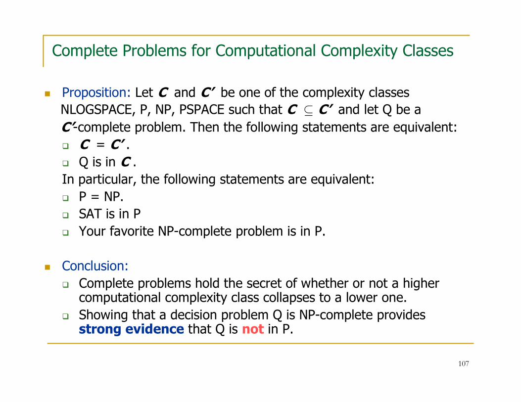
Complete Problems for Computational Complexity Classes
� Proposition: Let C and C’ be one of the complexity classes
NLOGSPACE, P, NP, PSPACE such that C ⊆ C’ and let Q be a
C’-complete problem. Then the following statements are equivalent:
� C = C’ .
� Q is in C .
In particular, the following statements are equivalent:
� P = NP.
� SAT is in P
� Your favorite NP-complete problem is in P.
� Conclusion:
� Complete problems hold the secret of whether or not a higher computational complexity class collapses to a lower one.
� Showing that a decision problem Q is NP-complete provides strong evidence that Q is not in P.
108
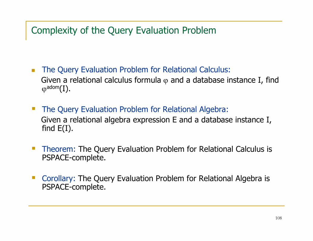
Complexity of the Query Evaluation Problem
� The Query Evaluation Problem for Relational Calculus:
Given a relational calculus formula ϕ and a database instance I, find ϕadom(I).
� The Query Evaluation Problem for Relational Algebra:
Given a relational algebra expression E and a database instance I, find E(I).
� Theorem: The Query Evaluation Problem for Relational Calculus is PSPACE-complete.
� Corollary: The Query Evaluation Problem for Relational Algebra is PSPACE-complete.
109
Complexity of the Query Evaluation Problem
� Theorem: The Query Evaluation Problem for Relational Calculus is PSPACE-complete.
Proof: We need to show that
� This problem is in PSPACE (i.e., give a PSPACE-algorithm for it).
� This problem is PSPACE-hard.
We start with the second task.

110
Complexity of the Query Evaluation Problem
� Theorem: The Query Evaluation Problem for Relational Calculus is PSPACE-hard.
� Proof: Show that
Quantified Boolean Formulas ≼p Query Evaluation for Rel. Calc.
Given QBF ∀ x1∃ x2 …. ∀ xk ψ
� Let V and P be two unary relation symbols
� Obtain ψ* from ψ by replacing xi by P(xi), and ¬xi by ¬P(xi)
� Let I be the database instance with V = {0,1}, P={1}.
� Then the following statements are equivalent:
� ∀ x1∃ x2 …. ∀ xk ψ is true
� ∀ x1 (V(x1) → ∃ x2 (V(x2)Æ(… ∀ xk(V(xk) → ψ*))…) is true on I.

111
Complexity of the Query Evaluation Problem
� Theorem: The Query Evaluation Problem for Relational Calculus is in PSPACE.
Proof (Hint): Let ϕ be a relational calculus formula ∀x1∃x2 … ∀xmψ and let I be a database instance.
� Exponential Time Algorithm: We can find ϕadom(I), by exhaustively cycling over all possible interpretations of the xi’s.
This runs in time O(nm), where n = |I| (size of I).
� A more careful analysis shows that this algorithm can be implemented in O(m�logn)-space.
� Use m blocks of memory, each holding one of the n elements of adom(I) written in binary (so O(logn) space is used in each block).
� Maintain also m counters in binary to keep track of the number of elements examined.
am in adom(I) written in binary
…a2 in adom(I) written in binary
a1 in adom(I) written in binary
∀ xm…∃ x2∀ x1

112
Complexity of the Query Evaluation Problem
� Corollary: The Query Evaluation Problem for Relational Algebra is PSPACE-complete.
Proof: The translation of relational calculus to relational algebra yields a polynomial-time reduction of the Query Evaluation Problem for Relational Calculus to the Query Evaluation Problem for Relational Algebra.

113
Summary
� The Query Evaluation Problem for Relational Calculus is PSPACE-complete.
� The Query Equivalence Problem for Relational Calculus in undecidable.
� The Query Containment Problem for Relational Calculus is undecidable.

114
Computational Complexity Classes
Classification of Decidable Problems
(not on scale)
There are many other complexity
classes. For a comprehensive catalog,
visit the Complexity Zoo at
qwiki.stanford.edu/wiki/Complexity_Zoo
LOGSPACE
NLOGSPACE
P
NP
PSPACE
.
.
.

115
Complete Problems
� A key property of most complexity classes is that they possess complete problems.
� Intuitively, complete problems are the “hardest” problems in the class in the sense that every other problem can be reduced to it.
� Definition: Let C be a complexity class.
A decision problem Q is C-complete if
� Q is in C.
� If Q’ is in C , then there is a “suitable” total Turing computable function f such that for every string x, we have that
x ∈ Q’ ⇔ f(x) ∈ Q.
� “suitable” means that f can be computed with fewer resources than those used to define C.
� So, f is a reduction of a restricted nature.

116
Complete Problems and Reductions
� Definition: A decision problem Q is NP-complete if
� Q is in NP.
� If Q’ is in NP, then there is a polynomial-time computable function f such that for every string x, we have that
x ∈ Q’ ⇔ f(x) ∈ Q.
� Such an f is a polynomial-time reduction of L to L* (L ≼p L*)
Logspace-computableNL
Logspace-computableP
Polynomial-time computableNP
Polynomial-time computablePSPACE
Reductions for Complete Problems
Complexity Class
117
The Query Evaluation Problem Revisited
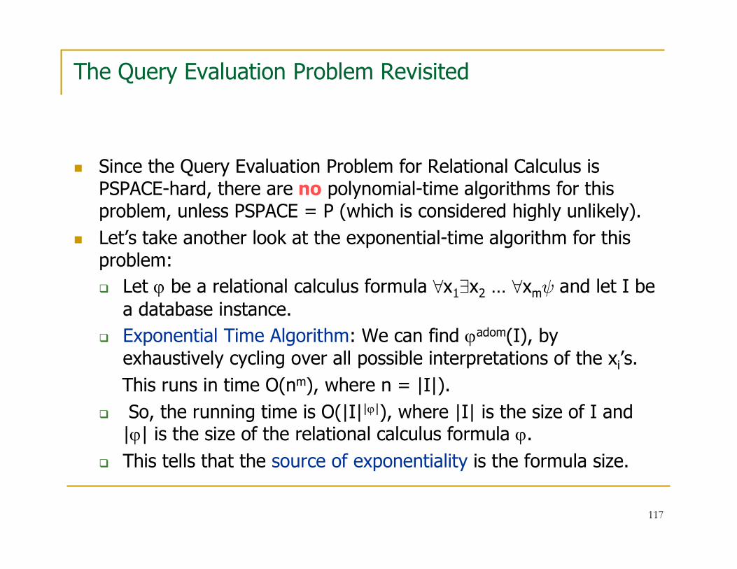
� Since the Query Evaluation Problem for Relational Calculus is PSPACE-hard, there are no polynomial-time algorithms for this problem, unless PSPACE = P (which is considered highly unlikely).
� Let’s take another look at the exponential-time algorithm for this problem:
� Let ϕ be a relational calculus formula ∀x1∃x2 … ∀xmψ and let I be a database instance.
� Exponential Time Algorithm: We can find ϕadom(I), by exhaustively cycling over all possible interpretations of the xi’s.
This runs in time O(nm), where n = |I|).
� So, the running time is O(|I||ϕ|), where |I| is the size of I and |ϕ| is the size of the relational calculus formula ϕ.
� This tells that the source of exponentiality is the formula size.

118
The Query Evaluation Problem Revisited
� Theorem: Let ϕ be a fixed relational calculus formula. Then the following problem is solvable in polynomial time: given a database instance I, find ϕadom(I). In fact, this problem is in LOGSPACE.
� Proof: Let ϕ be a fixed relational calculus formula ∀x1∃x2 … ∀xmψ
� The previous algorithm has running time O(|I||ϕ|), which is a polynomial, since now |ϕ| is a constant.
� Moreover, the algorithm can now be implemented using logarithmic-space only, since we need only maintain a constant number of memory blocks, each of logarithmic size
am in adom(I) written in binary
…a2 in adom(I) written in binary
a1 in adom(I) written in binary
∀ xm…∃ x2∀ x1

119
Vardi’s Taxonomy of the Query Evaluation Problem
M.Y Vardi, “The Complexity of Relational Query Languages”, 1982
� Definition: Let L be a database query language.
� The combined complexity of L is the decision problem:
given an L-sentence and a database instance I, is ϕ true on I? (does I satisfy ϕ?) (in symbols, does I � ϕ?)
� The data complexity of L is the family of the following decision problems Qϕ, where ϕ is an L-sentence: given a database instance I, does I � ϕ?
� The query complexity of L is the family of the following decision problems QI, where I is a database instance: given an L-sentence ϕ, does I � ϕ?
120
Vardi’s Taxonomy of the Query Evaluation Problem
Note: Let L be a database query language
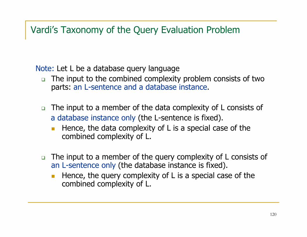
� The input to the combined complexity problem consists of two parts: an L-sentence and a database instance.
� The input to a member of the data complexity of L consists of
a database instance only (the L-sentence is fixed).
� Hence, the data complexity of L is a special case of the combined complexity of L.
� The input to a member of the query complexity of L consists of an L-sentence only (the database instance is fixed).
� Hence, the query complexity of L is a special case of the combined complexity of L.

121
Vardi’s Taxonomy of the Query Evaluation Problem
� Definition: Let L be a database query language and let C be a computational complexity class.� The data complexity of L is in C if for each L-sentence ϕ, the
decision problem Qϕ is in C.
� The query complexity of L is in C if for every database instance, the decision problem QI is in C.
� Vardi’s discovery:For most query languages L:
� The data complexity of L is of lower complexity than both the combined complexity of L and the query complexity of L
� The query complexity of L can be as hard as the combined complexity of L.

122
Taxonomy of the Query Evaluation Problem for Relational Calculus
Computational Complexity Classes
In LOGSPACEData Complexity
� Is in PSPACE
� It can be PSPACE-complete
Query Complexity
PSPACE-completeCombined Complexity
ComplexityProblem
LOGSPACE
NLOGSPACE
P
NP
PSPACE
.
.
.
The Query Evaluation Problem for Relational Calculus

123
The Query Evaluation Problem for Relational Calculus
� Paradox:
� The Query Evaluation Problem for Relational Calculus has
very high combined complexity
(PSPACE-complete, so “harder” than NP-complete).
� Yet, database systems evaluate SQL queries “efficiently”.
� Resolution of the Paradox:
� In practice, we deal with the data complexity of the Query Evaluation Problem for Relational Calculus, because we typicallyhave a small fixed collection of queries to answer (while of course the database instances vary).
� The data complexity of the Query Evaluation Problem for Relational Calculus is in LOGSPACE (hence, in PTIME); so, in principle, it is a tractable problem.

124
Sublanguages of Relational Calculus
� Question: Are there interesting sublanguages of relational calculus for which the Query Containment Problem and the Query EvaluationProblem are “easier” than the full relational calculus?
� Answer:
� Yes, the language of conjunctive queries is such a sublanguage.
� Moreover, conjunctive queries are the most frequently asked queries against relational databases.
125
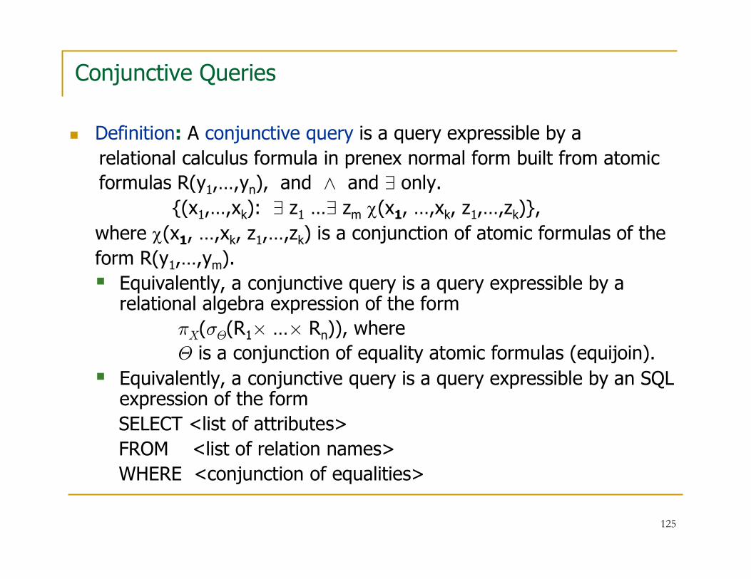
Conjunctive Queries
� Definition: A conjunctive query is a query expressible by a
relational calculus formula in prenex normal form built from atomic
formulas R(y1,…,yn), and Æ and ∃ only.
{(x1,…,xk): ∃ z1 …∃ zm χ(x1, …,xk, z1,…,zk)},
where χ(x1, …,xk, z1,…,zk) is a conjunction of atomic formulas of the
form R(y1,…,ym).
� Equivalently, a conjunctive query is a query expressible by a relational algebra expression of the form
πX(σΘ(R1× …× Rn)), where
Θ is a conjunction of equality atomic formulas (equijoin).
� Equivalently, a conjunctive query is a query expressible by an SQL expression of the form
SELECT <list of attributes>
FROM <list of relation names>
WHERE <conjunction of equalities>

126
Conjunctive Queries
� Definition: A conjunctive query is a query expressible by a
relational calculus formula in prenex normal form built from atomic
formulas R(y1,…,yn), and Æ and ∃ only.
{(x1,…,xk): ∃ z1 …∃ zm χ(x1, …,xk, z1,…,zk)}
� A conjunctive query can be written as a logic-programming rule:
Q(x1,…,xk) :-- R1(u1), …, Rn(un), where
� Each variable xi occurs in the right-hand side of the rule.
� Each ui is a tuple of variables (not necessarily distinct)
� The variables occurring in the right-hand side (the body), but not in the left-hand side (the head) of the rule are existentially quantified (but the quantifiers are not displayed).
� “,” stands for conjunction.

127
Conjunctive Queries
Examples:� Path of Length 2: (Binary query)
{(x,y): ∃ z (E(x,z) Æ E(z,y))}
� As a relational algebra expression, π1,4(σ$2 = $3 (E×E))
� As a rule:q(x,y) :-- E(x,z), E(z,y)
� Cycle of Length 3: (Boolean query)∃ x∃ y∃ z(E(x,y) Æ E(y,z) Æ E(z,x))
� As a rule (the head has no variables)� Q :-- E(x,z), E(z,y), E(z,x)

128
Conjunctive Queries
� Every relational join is a conjunctive query:
P(A,B,C), R(B,C,D) two relation symbols
� P ⋈ R = {(x,y,z,w): P(x,y,z) Æ R(y,z,w)}
� q(x,y,z,w) :-- P(x,y,z), R(y,z,w)
(no variables are existentially quantified)
� SELECT P.A, P.B, P.C, R.D
FROM P, R
WHERE P.B = R.B AND P.C = R.C
� Conjunctive queries are also known as SPJ-queries
(SELECT-PROJECT-JOIN queries)

129
Conjunctive Query Evaluation and Containment
� Definition: Two fundamental problems about CQs
� Conjunctive Query Evaluation (CQE):
Given a conjunctive query q and an instance I, find q(I).
� Conjunctive Query Containment (CQC):
� Given two k-ary conjunctive queries q1 and q2,
is it true that q1 ⊆ q2?
(i.e., for every instance I, we have that q1(I) ⊆ q2(I))
� Given two Boolean conjunctive queries q1and q2, is it true that q1 � q2? (that is, for all I, if I � q1, then I � q2)?
CQC is logical implication.

130
CQE vs. CQC
� Recall that for relational calculus queries:
� The Query Evaluation Problem is PSPACE-complete
(combined complexity).
� The Query Containment Problem is undecidable.
� Theorem: Chandra & Merlin, 1977
� CQE and CQC are the “same” problem.
� Moreover, each is an NP-complete problem.
� Question: What is the common link?
� Answer: The Homomorphism Problem
131
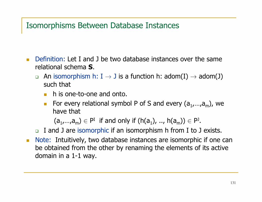
Isomorphisms Between Database Instances
� Definition: Let I and J be two database instances over the same relational schema S.
� An isomorphism h: I → J is a function h: adom(I) → adom(J) such that
� h is one-to-one and onto.
� For every relational symbol P of S and every (a1,…,am), we have that
(a1,…,am) ∈ PI if and only if (h(a1), .., h(am)) ∈ PJ.
� I and J are isomorphic if an isomorphism h from I to J exists.
� Note: Intuitively, two database instances are isomorphic if one can be obtained from the other by renaming the elements of its active domain in a 1-1 way.
132
A Digression to The Isomorphism Problem
� The Isomorphism Problem: Given two database instances I and J over the same relational schema, is I isomorphic to J?
� Fact: The exact computational complexity of the isomorphism problem is not known at present.
� The isomorphism problem is in NP (this is easy).
� The isomorphism problem is not known to be NP-complete
(and there is evidence that it is not NP-complete).
� The isomorphism problem is not known to be in P.
Finding a polynomial-time algorithm for the isomorphism problem would be a major breakthrough.
� Special cases of the isomorphism problem are known to be in P (for example, the isomorphism problem on planar graphs).

133
Homomorphisms
� Definition: Let I and J be two database instances over the same relational schema S. A homomorphism h: I → J is a function h: adom(I) → adom(J) such That for every relational symbol P of S and every (a1,…,am), wehave that
if (a1,…,am) ∈ PI , then (h(a1), .., h(am) ∈ PJ.
� Note: The concept of homomorphism is a relaxation of the concept of isomorphism, since every isomorphism is also a homomorphism, but not vice versa.
� Example:� A graph G = (V,E) is 3-colorable
if and only ifthere is a homomorphism h: G → K3

134
Homomorphisms
� Fact: Homomorphisms compose, i.e.,
if f: I → J and g: J → K are homomorphisms, then
g◦f: I → K is a homomorphims, where g◦f(a) = g(f(a)).
� Definition:
� Two database instances I and I’ are homomorphically equivalentif there is a homomorphism h: I → I’ and a homomorphism h’: I’ → I.
� I ≡h I’ means that I and I’ are homomorphically equivalent.
� Note: I ≡h I’ does not imply that I and I’ are isomorphic.
135
Homomorphisms
� Fact: Homomorphisms compose, i.e.,
if f: I → J and g: J → K are homomorphisms, then
g◦f: I → K is a homomorphims, where g◦f(a) = g(f(a)).
� Definition:
� Two database instances I and I’ are homomorphically equivalentif there is a homomorphism h: I → I’ and a homomorphism h’: I’ → I.
� I ≡h I’ means that I and I’ are homomorphically equivalent.
� Note: I ≡h I’ does not imply that I and I’ are isomorphic.
I I’

136
The Homomorphism Problem
� Definition: The Homomorphism ProblemGiven two database instances I and J, is there a homomorphismh: I → J?
� Notation: I → J denotes that a homomorphism from I to J exists.
� Theorem: The Homomorphism Problem is NP-completeProof: Easy reduction from 3-ColorabiltyG is 3-colorable if and only if G → K3.
� Exercise: Formulate 3SAT as a special case of the Homomorphism Problem.

137
The Homomorphism Problem
� Note: The Homomorphism Problem is a fundamental algorithmic problem:
� Satisfiability can be viewed as a special case of it.
� k-Colorability can be viewed as a special case of it.
� Many AI problems, such as planning, can be viewed as a special case of it.
� In fact, every constraint satisfaction problem can be viewed as a special case of the Homomorphism Problem
(Feder and Vardi – 1993).
138
The Homomorphism Problem and Conjunctive Queries
� Theorem: Chandra & Merlin, 1977
� CQE and CQC are the “same” problem.
� Moreover, each is an NP-complete problem.
� Question: What is the common link?
� Answer:
� Both CQE and CQC are “equivalent” to the Homomorphism Problem.
� The link is established by bringing into the picture
� Canonical conjunctive queries and
� Canonical database instances.

139
Canonical CQs and Canonical Instances
� Definition: Canonical Conjunctive QueryGiven an instance I = (R1, …,Rm), the canonical CQ of I is the Boolean conjunctive query QI with (a renaming of) the elements of I as variables and the facts of I as conjuncts, where a fact of I is an expressionRi(a1,…,am) such that (a1,…,am) ∈ Ri.
� Example:I consists of E(a,b), E(b,c), E(c,a)
� QI is given by the rule:QI :-- E(x,z), E(z,y), E(y,x)
� Alternatively, QI is ∃ x ∃ y ∃ z (E(x,z) Æ E(z,y) Æ E(y,x))
140
Canonical Conjunctive Query
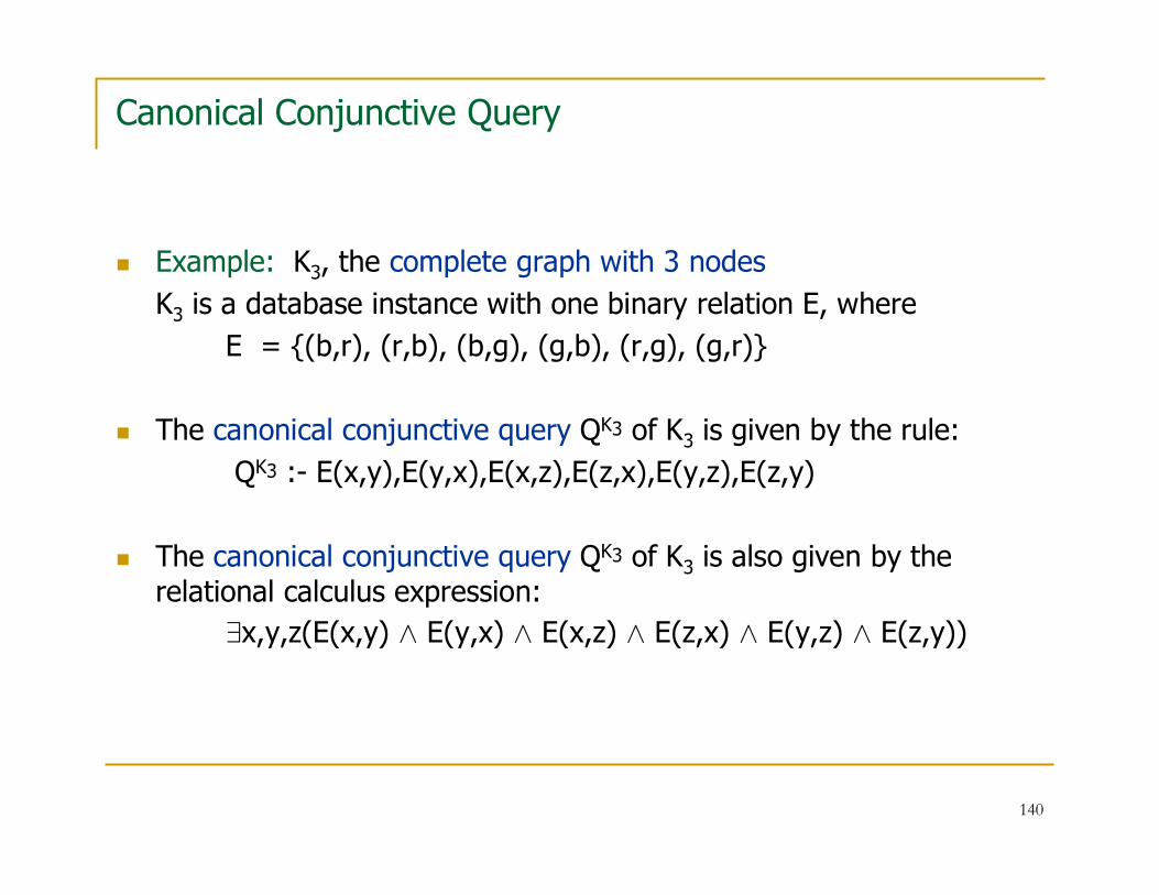
� Example: K3, the complete graph with 3 nodes
K3 is a database instance with one binary relation E, where
E = {(b,r), (r,b), (b,g), (g,b), (r,g), (g,r)}
� The canonical conjunctive query QK3 of K3 is given by the rule:
QK3 :- E(x,y),E(y,x),E(x,z),E(z,x),E(y,z),E(z,y)
� The canonical conjunctive query QK3 of K3 is also given by the relational calculus expression:
∃x,y,z(E(x,y) Æ E(y,x) Æ E(x,z) Æ E(z,x) Æ E(y,z) Æ E(z,y))
141
Canonical Database Instance
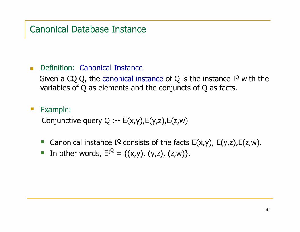
� Definition: Canonical Instance
Given a CQ Q, the canonical instance of Q is the instance IQ with the variables of Q as elements and the conjuncts of Q as facts.
� Example:
Conjunctive query Q :-- E(x,y),E(y,z),E(z,w)
� Canonical instance IQ consists of the facts E(x,y), E(y,z),E(z,w).
� In other words, EIQ = {(x,y), (y,z), (z,w)}.

142
Canonical Database Instance
� Example:
Conjunctive query Q(x,y) :-- E(x,z),E(z,y),P(z)
or, equivalently,
{(x,y): ∃ z(E(x,z)Æ E(z,y)Æ P(z)}
� Canonical instance IQ consists of the facts
E(x,z), E(z,y),P(z).
� In other words, EIQ = {(x,z), (z,y)} and PIQ={z}
143
Canonical Conjunctive Queries and Canonical Instances
� Fact:� For every database instance I, we have that I � QI.
� For every Boolean conjunctive query Q, we have that IQ � Q.
� Fact: Let I be a database instance, let QI be its canonical
conjunctive query and let IQIbe the canonical instance of QI.
Then I is isomorphic to IQI.

144
Canonical Conjunctive Queries and Canonical Instances
Magic Lemma: Assume that Q is a Boolean conjunctive query and J is a
database instance. Then the following statements are equivalent.� J � Q.
� There is a homomorphism h: IQ → J.
Proof: Let Q be ∃ x1 …∃ xm ϕ(x1,…,xm).
1. ⇒ 2. Assume that J � Q. Hence, there are elements
a1, …, am in adom(J) such that J � ϕ(a1,…,am). The function h with
h(xi) = ai, for i=1,…,m, is a homomorphism from IQ to J.
2. ⇒ 1. Assume that there is a homomorphism h: IQ → J.
Then the values h(xi) = ai, for i = 1,…, m, give values for the
interpretation of the existential quantifiers ∃ xi of Q in adom(J) so that J � ϕ(a1,…,am).

145
Homomorphisms, CQE, and CQC
The Homomorphism Theorem: Chandra & Merlin – 1977
For Boolean CQs Q and Q’, the following are equivalent:
� Q ⊆ Q’
� There is a homomorphism h: IQ’ → IQ
� IQ � Q’.
In dual form:
The Homomorphism Theorem: Chandra & Merlin – 1977
For instances I and I’, the following are equivalent:
� There is a homomorphism h: I → I’� I’ � QI
� QI’ ⊆ QI

146
Homomorphisms, CQE, and CQC
The Homomorphism Theorem: Chandra & Merlin – 1977
For Boolean CQs Q and Q’, the following are equivalent:
1. Q ⊆ Q’
2. There is a homomorphism h: IQ’ → IQ
3. IQ � Q’.
Proof:
1. ⇒ 2. Assume Q ⊆ Q’. Since IQ � Q, we have that IQ � Q’.
Hence, by the Magic Lemma, there is a homomorphism from IQ’ to IQ.
2. ⇒ 3. It follows from the other direction of the Magic Lemma.
3. ⇒ 1. Assume that IQ � Q’. So, by the Magic Lemma, there is a
homomorphism h: IQ’ → IQ. We have to show that if J � Q, then J � Q’. Well, if
J � Q, then (by the Magic Lemma), there is a homomorphism h’: IQ → J. The
composition h’◦ h: IQ’ → J is a homomorphism, hence
(once again by the Magic Lemma!), we have that J � Q’.
147
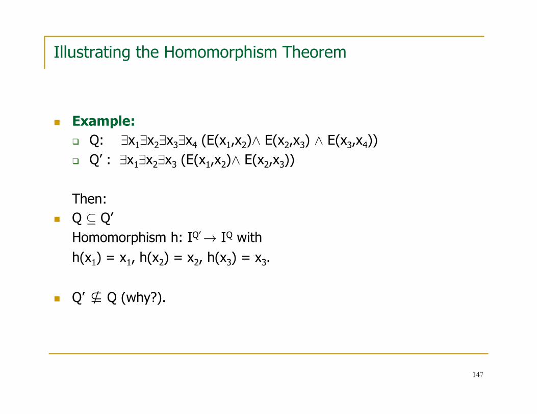
Illustrating the Homomorphism Theorem
� Example:
� Q: ∃x1∃x2∃x3∃x4 (E(x1,x2)Æ E(x2,x3) Æ E(x3,x4))
� Q’ : ∃x1∃x2∃x3 (E(x1,x2)Æ E(x2,x3))
Then:
� Q ⊆ Q’
Homomorphism h: IQ’→ IQ with
h(x1) = x1, h(x2) = x2, h(x3) = x3.
� Q’ ⊈ Q (why?).
148
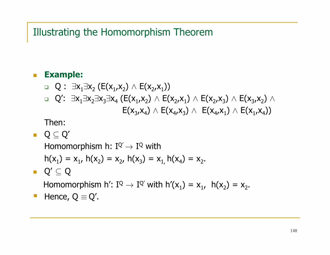
Illustrating the Homomorphism Theorem
� Example:
� Q : ∃x1∃x2 (E(x1,x2) Æ E(x2,x1))
� Q’: ∃x1∃x2∃x3∃x4 (E(x1,x2) Æ E(x2,x1) Æ E(x2,x3) Æ E(x3,x2) Æ
E(x3,x4) Æ E(x4,x3) Æ E(x4,x1) Æ E(x1,x4))
Then:
� Q ⊆ Q’
Homomorphism h: IQ’→ IQ with
h(x1) = x1, h(x2) = x2, h(x3) = x1, h(x4) = x2.
� Q’ ⊆ Q
Homomorphism h’: IQ → IQ’ with h’(x1) = x1, h(x2) = x2.
� Hence, Q ≡Q’.

149
Illustrating the Homomorphism Theorem
Example: 3-Colorability
For a graph G=(V,E), the following are equivalent:
� G is 3-colorable
� There is a homomorphism h: G → K3
� K3 � QG
� QK3 ⊆ QG.

150
The Homomorphism Theorem for non-Boolean Conjunctive Queries
� So far, we have focused on Boolean conjunctive queries.
� However, the Homomorphism Theorem easily extends to conjunctive queries of arbitrary arities by considering homomorphisms that are the identity on the variables in the head of the conjunctive queries (written as rules).
� Moreover, the Homomorphism Theorem also extends to conjunctive queries with constants in some of the conjuncts.
Find all cities one can reach by flying from San Jose with two stops
{x: ∃x1∃x2 (FLIGHT(SanJose, x1)Æ FLIGHT(x1,x2) Æ FLIGHT(x2,x))}.

151
The Homomorphism Theorem for non-Boolean Conjunctive Queries
The Homomorphism Theorem: Chandra & Merlin – 1977
Consider two k-ary conjunctive queries
Q(x1,…,xk) :-- R1(u1), …, Rn(un) and Q’(x1,…,xk) :-- T1(v1), …, Tm(vm),
Then the following are equivalent:
� Q ⊆ Q’
� There is a homomorphism h: IQ’ → IQ such that
h(x1) = x1, h(x2) = x2, …, h(xk) = xk.
� IQ, x1,…, xk � Q’.

152
The Homomorphism Theorem for non-Boolean Conjunctive Queries
� Example: Consider the binary conjunctive queries
Q(x,y):-- E(y,x),E(x,u)
and
Q’(x,y) :-- E(y,x), E(z,x),E(w,x),E(x,u)
Then Q ⊆ Q’ because there is a homomorphism
h: IQ’ → IQ with h(x) =x and h(y) = y,
namely,
h(x) = x, h(y) = y, h(z) =y, h(w) = y, h(u) = u.
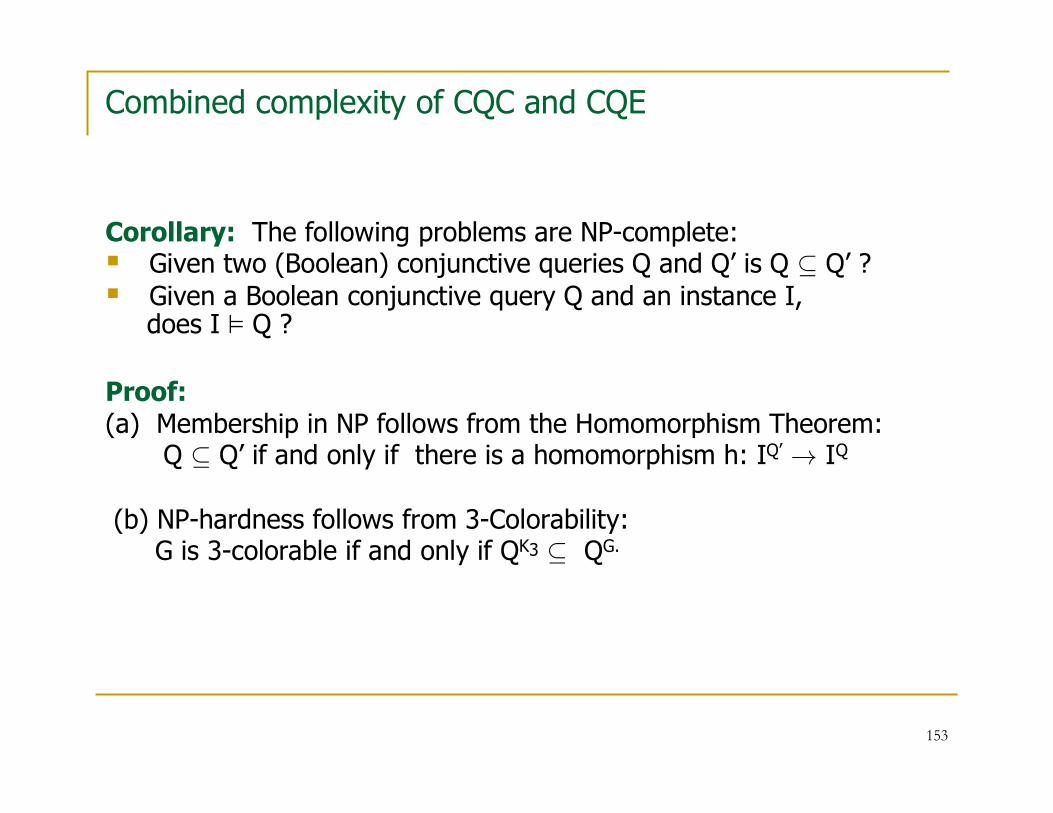
153
Combined complexity of CQC and CQE
Corollary: The following problems are NP-complete:� Given two (Boolean) conjunctive queries Q and Q’ is Q ⊆ Q’ ?� Given a Boolean conjunctive query Q and an instance I,
does I � Q ?
Proof:(a) Membership in NP follows from the Homomorphism Theorem:
Q ⊆ Q’ if and only if there is a homomorphism h: IQ’ → IQ
(b) NP-hardness follows from 3-Colorability:G is 3-colorable if and only if QK3 ⊆ QG.

154
Conjunctive Query Equivalence
� The Conjunctive Query Equivalence Problem: Given two conjunctive queries Q and Q’, is Q ≡ Q’?
� Corollary: For conjunctive queries Q and Q’, we have that
Q ≡ Q’ if and only if IQ ≡h IQ’.
� Corollary: The Conjunctive Query Equivalence Problem is
NP-complete.
� Proof:
� The following problem is NP-complete:
Given a graph H containing a K3, is H 3-colorable?
� Let H be a graph containing a K3. Then
H is 3-colorable if and only if QH ≡ QK3.
155
Combined Complexity vs. Data Complexity
Recall Vardi’s Taxonomy of Query Evaluation:
� Combined Complexity: Both the query and the instance are part of the input.
� Data Complexity: Fix the query; the input consists of the instance only.
Complexity of Conjunctive Query Evaluation:
� The combined complexity of conjunctive query evaluation is
NP-complete.
� The data complexity of conjunctive query evaluation is in P
(in fact, it is in LOGSPACE).

156
The Complexity of Database Query Languages
NP-completeUndecidableQuery Containment Problem
NP-completeUndecidableQuery Equivalence Problem
In LOGSPACE
(hence, in P)
In LOGSPACE
(hence, in P)
Query Evaluation Problem:
Data Complexity
NP-completePSPACE-completeQuery Evaluation Problem: Combined Complexity
Conjunctive QueriesRelational Calculus

157
Conjunctive Query Minimization
� Definition: Let Q be a conjunctive query. A minimal equivalent conjunctive query to Q is a conjunctive query Q’ such that
� Q is equivalent to Q’;
� Q’ has as few conjuncts as any conjunct. query equivalent to Q.
� Example: Let Q be the conjunctive query
Q(x,y) :-- E(y,x), E(z,x),E(w,x),E(x,u)
Then the conjunctive query
Q’(x,y):-- E(y,x),E(x,u)
is a minimal equivalent conjunctive query to Q. (Why?)

158
Conjunctive Query Minimization and Conjunctive Query Evaluation
� A natural approach to conjunctive query evaluation is to first process a given conjunctive query Q, transform it to a minimal equivalent conjunctive query Q’, and then evaluate Q’ instead of Q.
� At first sight, this seems to be a promising approach.
� There is good news and bad news. First, the good news:
� Theorem: Let Q be a conjunctive query.
� There is a minimal equivalent conjunctive query Q’ obtained from Q by removing zero or more conjuncts.
� All minimal equivalent conjunctive queries to Q are isomorphic, i.e., their canonical instances are all isomorphic to each other.
Proof: Use the Homomorphism Theorem (exercise).

159
Conjunctive Query Minimization and Conjunctive Query Evaluation
Next, the bad news:
Theorem:
� The following problem is NP-hard: Given two conjunctive queries Q and Q’, is Q’ a minimal equivalent query to Q?
� Consequently, unless P = NP, there is no polynomial-time algorithm such that, given a conjunctive query Q, the algorithm outputs a conjunctive query Q’ that is a minimal equivalent query to Q.
Proof: Reduction from 3-Colorability (exercise).
Note:
� This is not surprising since, as we saw, conjunctive query evaluation is NP-complete.
� There is an exponential-time algorithm such that, given a conjunctive query Q, the algorithm outputs a conjunctive query Q’that is a minimal equivalent query to Q.

160
Tractable Cases of Conjunctive Query Evaluation
� Since conjunctive query evaluation is NP-complete, there has been an extensive investigation of special cases of conjunctive queryevaluation for which the problem is in P.
� The key idea is to impose structural restrictions on the conjunctive queries considered:
� Acyclic joins – M. Yannakakis (1981)
� Various extensions of acyclicity have been studied over the years,
including queries of bounded tree-width and queries of bounded hypertree width.
� Extensive interaction with constraint satisfaction, logic, and graph theory.
� This belongs more to an advanced topics course or an independentstudy course.
161
Beyond Conjunctive Queries
� What can we say about query languages of intermediate expressivepower between conjunctive queries and the full relational calculus?
� Conjunctive queries form the sublanguage of relational algebra obtained by using only cartesian product, projection, and selection with equality conditions.
� The next step would be to consider relational algebra expressions that also involve union.

162
Beyond Conjunctive Queries
� Definition:
� A union of conjunctive queries is a query expressible by an expression of the form q1 ∪ q2 ∪ … ∪ qm, where each qi is a conjunctive query.
� A monotone query is a query expressible by a relational algebra expression which uses only union, cartesian product, projection, and selection with equality condition.
� Fact:
� Every union of conjunctive queries is a monotone query.
� Every monotone query is equivalent to a union of conjunctive queries, but the union may have exponentially many disjuncts.
(normal form for monotone queries).
� Monotone queries are precisely the queries expressible by relational calculus expressions using Æ, Ç, and ∃ only.

163
Unions of Conjunctive Queries and Monotone Queries
� Union of Conjunctive Queries
E ∪ π1,4 (σ$2=$3 (E× E)) or, as a relational calculus expression,
E(x1,x2) Ç ∃ z(E(x1,z)Æ E(z,x2))
� Monotone Query
Consider the relation schemas R1(A,B), R2(A,B), R3(B,C), R4(B,C).
The monotone query
(R1 ∪ R2) ⋈ (R3 ∪ R4)
is equivalent to the following union of conjunctive queries:
(R1 ⋈ R3) ∪ (R1 ⋈ R4) ∪ (R2 ⋈ R3) ∪ (R2 ⋈ R4).

164
The Containment Problem for Unions of Conjunctive Queries
Theorem: Sagiv and Yannakakis – 1981
Let q1 ∪ q2 ∪ … ∪ qm and q’1 ∪ q’2 ∪ … ∪ q’n be two unions of
conjunctive queries. Then the following are equivalent:
1. q1 ∪ q2 ∪ … ∪ qm ⊆ q’1 ∪ q’2 ∪ … ∪ q’n.
2. For every i ≤ m, there is j ≤ n such that qi ⊆ q’j.
Proof: Use the Homomorphism Theorem
1. ⇒ 2. Since Iqi � qi, we have that Iqi � q1 ∪ q2 ∪ … ∪ qm , hence
Iqi � q’1 ∪ q’2 ∪ … ∪ q’n , hence there is some j ≤ n such that Iqi � q’j,
hence (by the Homomorphism Theorem) qi ⊆ q’j.
2. ⇒ 1. This direction is obvious.

165
The Containment Problem for Unions of Conjunctive Queries
� Corollary: The Query Containment Problem for
Unions of Conjunctive Queries is NP-complete.
� Proof:
� Membership in NP follows from the Sagiv-Yannakakis Theorem.
� We guess m pairs (q’ki, hki
) and verify that for every i ≤ m,
the function hkiis a homomorphism from Iq’ki to Iqi.
� NP-hardness follows from the fact that Conjunctive Query Containment is a special case of this problem.
� Fact: The Query Evaluation Problem for Unions of Conjunctive Queries is NP-complete (combined complexity).
Proof: Exercise.

166
The Complexity of Database Query Languages
NP-completeNP-completeUndecidableQuery Containment
NP-completeNP-completeUndecidableQuery Equivalence
In LOGSPACE
(hence, in P)
In LOGSPACE
(hence, in P)
In LOGSPACE
(hence, in P)
Query Evaluation:
Data Complexity
NP-completeNP-completePSPACE-completeQuery Evaluation: Combined Complexity
Unions of Conjunctive Queries
Conjunctive Queries
Relational Calculus
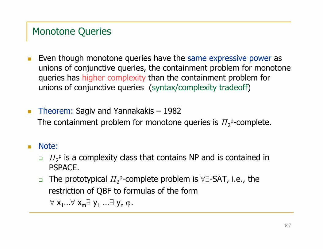
167
Monotone Queries
� Even though monotone queries have the same expressive power as unions of conjunctive queries, the containment problem for monotone queries has higher complexity than the containment problem for unions of conjunctive queries (syntax/complexity tradeoff)
� Theorem: Sagiv and Yannakakis – 1982
The containment problem for monotone queries is Π2p-complete.
� Note:
� Π2p is a complexity class that contains NP and is contained in
PSPACE.
� The prototypical Π2p-complete problem is ∀∃-SAT, i.e., the
restriction of QBF to formulas of the form
∀ x1…∀ xm∃ y1 …∃ yn ϕ.

168
The Complexity of Database Query Language
Π2p-completeNP-completeNP-completeUndecidableQuery
Containment
Π2p-completeNP-completeNP-completeUndecidableQuery
Equivalence
In LOGSPACE (hence, in P)
In LOGSPACE (hence, in P)
In LOGSPACE (hence, in P)
In LOGSPACE (hence, in P)
Query Eval.:
Data Complexity
NP-completeNP-completeNP-completePSPACE-complete
Query Eval.: Combined Complexity
Monotone Queries
Unions of Conjunctive Queries
Conjunctive Queries
Relational Calculus

169
Conjunctive Queries with Inequalities
� Definition: Conjunctive queries with inequalities form the
sublanguage of relational algebra obtained by using only cartesianproduct, projection, and selection with equality and inequality
(≠, <, ≤) conditions.
� Example: Q(x,y):-- E(x,z), E(z,w),E(w,y), z ≠ w, z < y.
� Theorem: (Klug – 1988, van der Meyden – 1992)
� The query containment problem for conjunctive queries with inequalities is Π2
p-complete.
� The query evaluation problem for conjunctive queries with inequalities in NP-complete.

170
The Complexity of Database Query Languages
Π2p-completeNP-completeNP-completeUndecidableQuery
Containment
Π2p-completeNP-completeNP-completeUndecidableQuery
Equivalence
In LOGSPACE (hence, in P)
In LOGSPACE (hence, in P)
In LOGSPACE (hence, in P)
In LOGSPACE (hence, in P)
Query Eval.:
Data Complexity
NP-completeNP-completeNP-completePSPACE-complete
Query Eval.: Combined Complexity
Monotone Queries/
Conj.Querieswith Inequal.
Unions of Conjunctive Queries
Conjunctive Queries
Relational Calculus

171
Conjunctive Queries with Inequalities
� Note: The Homomorphism Theorem fails for conjunctive queries with inequalities.
� Example: Consider the queries
� q(x,y) :- E(x,y), F(u,v)
� p(x,y) :- E(x,y), F(u,v), u ≠ v.
Then
� q(x,y) ⊈ p(x,y) (why?)
� Yet, Ip is the same as Iq;
in particular, there is a homomorphism h: Ip → Iq.
� Note also that p(x,y) ⊆ q(x,y) (why?)

172
Complexity of Query Containment
� So, the complexity of query containment for conjunctive queries and their variants is well understood.
Caveat:
� All preceding results assume set semantics, i.e., queries take sets as inputs and return sets as output (duplicates are eliminated).
� DBMS, however, use bag semantics (multiset semantics), since they return bags (multisets)
(recall that duplicates are not eliminated in SQL, unless explicitly specified).

173
A Real Conjunctive Query
� Consider the following SQL query:
Table Employee has attributes salary, dept, …
SELECT salaryFROM EmployeeWHERE dept = ‘CS’
� Recall that SQL keeps duplicates, because:
� User may care about duplicates
{100, 100, 200} different than {100, 200} for AVERAGE
� In general, bags can be more “efficient” than sets.

174
Query Evaluation under Bag Semantics
Duplicates are not eliminated
Projection and Selection
m1× m2Product
R1 × R2
min(m1, m2)Intersection
R1 R2
m1 + m2Union
R1 ∪ R2
MultiplicityOperation� R1 A B
1 21 2 2 3
� R2 B C2 42 5
� (R1 ⋈ R2) A B C
1 2 41 2 41 2 51 2 5

175
Bag (Multiset) Semantics
S. Chaudhuri & M.Y. Vardi – 1993
Optimization of Real Conjunctive Queries
� Called for a re-examination of conjunctive-query optimization under bag semantics.
� In particular, they initiated the study of the
containment problem for conjunctive queries under bag semantics.

176
Bag Semantics vs. Set Semantics
� QBAG(I) : Result of evaluating Q on (bag) database instance I.
� For bags R1, R2:
R1 ⊆BAG R2 if m(a,R1) ≤ m(a,R2), for every tuple a.
� Q1 ⊆BAG Q2 if for every (bag) database I, we have that
Q1BAG(I) ⊆BAG Q2
BAG(I).
Fact:
� Q1 ⊆BAG Q2 implies Q1 ⊆ Q2 (this is obvious from the definitions).
� The converse does not always hold.
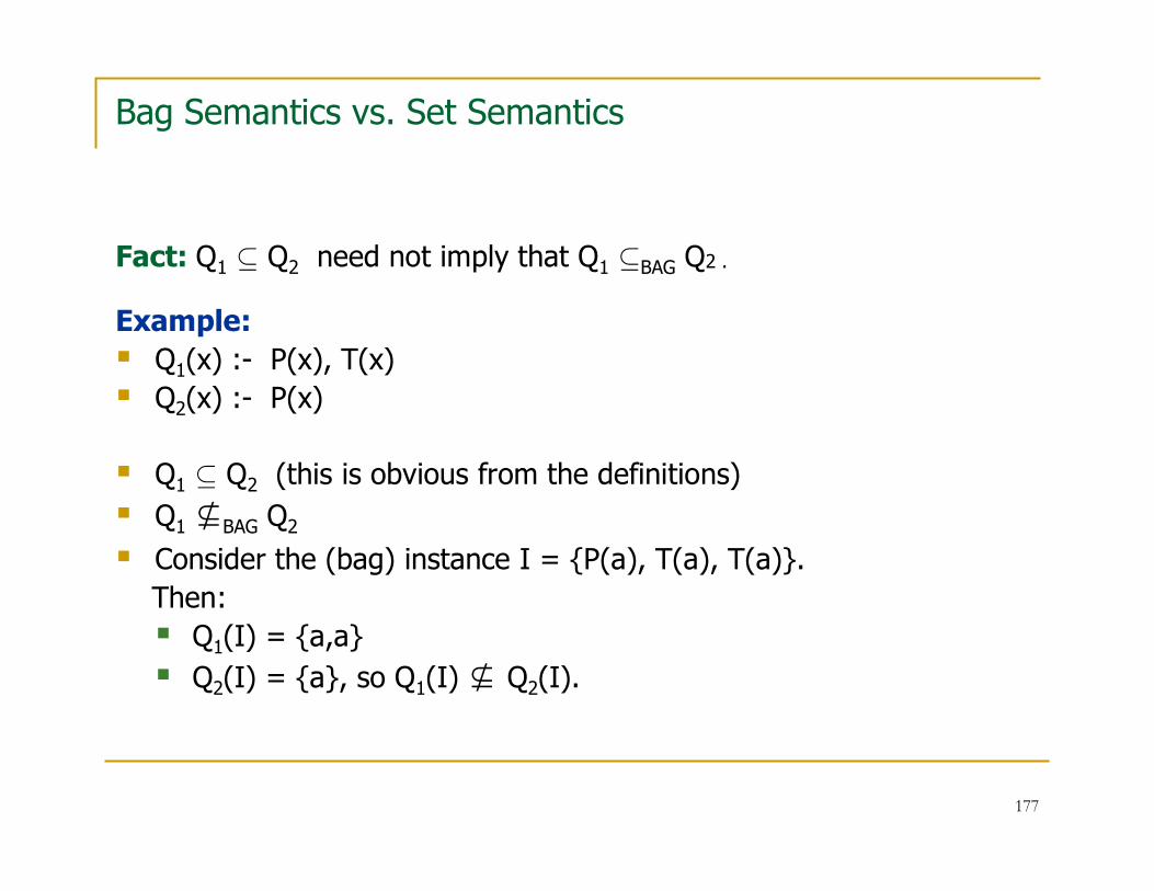
177
Bag Semantics vs. Set Semantics
Fact: Q1 ⊆ Q2 need not imply that Q1 ⊆BAG Q2 .
Example:
� Q1(x) :- P(x), T(x)
� Q2(x) :- P(x)
� Q1 ⊆ Q2 (this is obvious from the definitions)
� Q1 ⊈BAG Q2
� Consider the (bag) instance I = {P(a), T(a), T(a)}.
Then:
� Q1(I) = {a,a}
� Q2(I) = {a}, so Q1(I) ⊈ Q2(I).

178
Conjunctive Query Evaluation under Bag Semantics
� Boolean query
Q :- E(x,y), E(y,z), E(z,x)
� Set Semantics
Q(G) = “true” if and only if the graph G contains a triangle.
� Bag Semantics
QBAG(G) = # of triangles in the graph G.

179
Conjunctive Query Evaluation under Bag Semantics
Consider:
� K3: the complete graph with 3 nodes
� G=(V,E) an arbitrary graph and the canonical conjunctive query QG of G.
Then
� Set Semantics
QG(K3) = “true” if and only if G is 3-colorable.
� Bag Semantics
QG-BAG(K3) = # 3-colorings of the graph G.
Corollary: The conjunctive query evaluation problem under bag
semantics is #P-complete.

180
Query Containment under Bag Semantics
� Chaudhuri & Vardi - 1993 stated that:
Under bag semantics, the containment problem for conjunctivequeries is Π2
p-hard.
� Open Problem:
� What is the exact complexity, under bag semantics, of the containment problem for conjunctive queries?
� Is this problem decidable? Even this is not known to date!

181
Unions of Conjunctive Queries
Theorem: Ioannidis & Ramakrishnan – 1995
Under bag semantics, the containment problem for
unions of conjunctive queries is undecidable.
Hint of Proof:
Reduction from
Hilbert’s 10th Problem.

182
Hilbert’s 10th Problem
� Hilbert’s 10th Problem – 1900
(10th in his list of 23 problems)
Find an algorithm for the following problem:
Given a polynomial equation p(x1,...,xn) = 0 with integer coefficients, does it have an all-integer solution?
� Matijasevic – 1971
� Hilbert’s 10th Problem is undecidable, hence no such algorithm exists.
� Undecidable, even for degree d = 4 and n = 58.
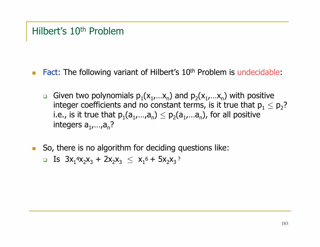
183
Hilbert’s 10th Problem
� Fact: The following variant of Hilbert’s 10th Problem is undecidable:
� Given two polynomials p1(x1,…xn) and p2(x1,…xn) with positive integer coefficients and no constant terms, is it true that p1 ≤ p2? i.e., is it true that p1(a1,…,an) ≤ p2(a1,…an), for all positive integers a1,…,an?
� So, there is no algorithm for deciding questions like:
� Is 3x14x2x3 + 2x2x3 ≤ x1
6 + 5x2x3?

184
Unions of Conjunctive Queries
Theorem: Ioannidis & Ramakrishnan – 1995
Under bag semantics, the containment problem for unions of
conjunctive queries is undecidable, even if all relations are unary.
Hint of Proof:
� Reduction from the previous variant of Hilbert’s 10th Problem:
� Use joins of unary relations to encode monomials (products of variables).
� Use unions to encode sums of monomials.

185
Unions of Conjunctive Queries
Theorem: Ioannidis & Ramakrishnan – 1995
Under bag semantics, the containment problem for unions of
conjunctive queries is undecidable, even if all relations are unary.
Example: Consider the polynomial 3x14x2x3 + 2x2x3
� The monomial x14x2x3 is encoded by the conjunctive query
P1(w),P1(w),P1(w), P
1(w), P2(w),P3(w).
� The monomial x2x3 is encoded by the conjunctive query P2(w),P3(w).
� The polynomial 3x14x2x3 + 2x2x3 is encoded by the union having:
� three copies of P1(w),P1(w),P1(w), P1(w), P2(w),P3(w) and
� two copies of P2(w),P3(w).

186
Computational Complexity of Query Containment
UndecidableUndecidable
Trakhtenbrot - 1949
Relational calculus queries
Π2p-complete
Van der Meyden – 1992
Conj. queries with
≠≠≠≠ , ≤, ≥
Undecidable
Ioannidis-Ramakrishnan -1995
NP-complete
Sagiv-Yannakakis – 1981
Unions of conj. queries
OpenNP-complete
Chandra Merlin – 1977
Conjunctive queries
Complexity –
Bag Semantics
Complexity –
Set Semantics
Class of Queries

187
Bag Semantics and Conjunctive Queries with g
Theorem: Jayram, K… , Vee – 2006
Under bag semantics, the containment problem for
conjunctive queries with g is undecidable.
In fact, this problem is undecidable even if
� the queries use only a single relation of arity 2;
� the number of inequalities in the queries is at most some fixed constant.

188
Bag Semantics and Conjunctive Queries with g
Proof Idea:
Reduction from another variant of Hilbert’s10th Problem:
Given homogeneous polynomials
P1(x1,…,x59) and P2(x1,…,x59)
both with integer coefficients and both of degree 5,
is P1(x1,…,x59) ≤ (x1)5 P2(x1,…,x59),
for all integers x1,…,x59?
The reduction is much more involved than the earlier reduction for
unions of conjunctive queries.

189
Proof Idea (continued)
� Given polynomials P1 and P2
� Both with integer coefficients
� Both homogeneous, degree 5
� Both with at most n=59 variables
� We want to find Q1 and Q2 such that
� Q1 and Q2 are conjunctive queries with inequalities g
� P1(x1,…, x59) ≤ (x1)5 P2(x1,…, x59)
for all integers x1, …, x59
if and only if
Q1(D) ⊆BAG
Q2(D) for all (bag) databases D.

190
Proof Outline:
Proof is carried out in three steps.
Step 1: Only consider DBs of a special form.
Show how to use conjunctive queries to encode
polynomials (without using inequalities!)
Step 2: “Force” DB to have special form using inequalities.
� If D is not of special form, thenQ1(D) ⊆BAG Q2(D) necessarily.
Step 3: Show that we only need a single relation of arity 2.
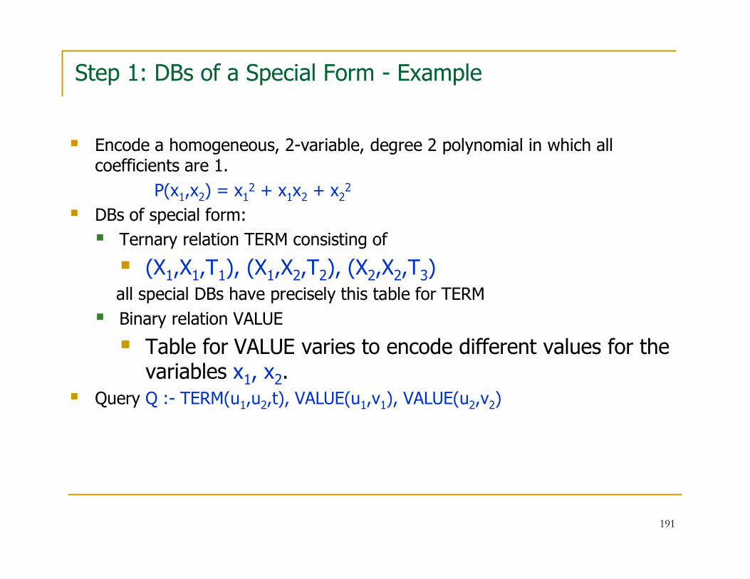
191
Step 1: DBs of a Special Form - Example
� Encode a homogeneous, 2-variable, degree 2 polynomial in which all coefficients are 1.
P(x1,x2) = x12 + x1x2 + x2
2
� DBs of special form:
� Ternary relation TERM consisting of
� (X1,X1,T1), (X1,X2,T2), (X2,X2,T3)all special DBs have precisely this table for TERM
� Binary relation VALUE
� Table for VALUE varies to encode different values for the variables x1, x2.
� Query Q :- TERM(u1,u2,t), VALUE(u1,v1), VALUE(u2,v2)

192
Step 1: DBs of a Special Form - Example
� P(x1,x2) = x12 + x1x2 + x2
2
x1 = 3, x2 = 2, P(3,2) = 32 + 3·2 + 22 = 19.
� Query Q :- TERM(u1,u2,t), VALUE(u1,v1), VALUE(u2,v2)
� DB D of special form:
� TERM: (X1,X1,T1), (X1,X2,T2), (X2,X2,T3)
� VALUE: (X1,1), (X1,2), (X1,3)
(X2,1), (X2,2)
Claim: P(3,2) = 19 = QBAG(D)

193
Step 1: DBs of a Special Form - Example
� P(3,2) = 32 + 3·2 + 22 = 19.
� Query Q :- TERM(u1,u2,t), VALUE(u1,v1), VALUE(u2,v2)
� D has TERM: (X1,X1,T1), (X1,X2,T2), (X2,X2,T3)
VALUE: (X1,1), (X1,2), (X1,3), (X2,1), (X2,2)
� QBAG(D) = 19, because:
� t → T1, u1→ X1, u2→ X1. Hence:
v1 → 1,2, or 3 and v2→ 1 or 2, so we get 32 witnesses.
� t → T2, u1→ X1, u2→ X2. Hence:
v1 → 1,2, or 3 and v2→ 1 or 2, so we get 3·2 witnesses.
� t → T3, u1→ X2, u2→ X2. Hence:
v1 → 1 or 2, and v2→ 1 or 2, so we get 22 witnesses.

194
Step 1: Complete Argument and Wrap-up
� Previous technique only works if all coefficients are 1
� For the complete argument:
� add a fixed table for every term to the DB;
� encode coefficients in the query;
� only table for VALUE can vary.
� Summary:
� If the database has a special form, then we can encode separately homogeneous polynomials
P1 and P2 by conjunctive queries Q1 and Q2.
� By varying table for VALUE, we vary the variable values.
� No ≠-constraints are used in this encoding; hence, conjunctive query containment is undecidable, if restricted to databases of the special form.

195
Step 2: Arbitrary Databases
Idea:
Use inequalities g in the encoding queries
to achieve the following:
� If a database D is of special form, then we are back to the previous case.
� If a database D is not of special form, thenQ1(D) ⊆BAG Q2(D) necessarily.

196
Step 2: Arbitrary Databases - Hint
1. Ensure that certain “facts” in special-form DBs appear
(else neither query is satisfied).
� This is done by adding a part of the canonical query of special-form DBs as subgoals to each encoding query.
2. Modify special-form DBs by adding gadget tuples to TERM and
to VALUE.
� TERM: (X1,X1,T1), (X1,X2,T2), (X2,X2,T3), (T0,T0,T0)
� VALUE: (X1,1), (X1,2), (X1,3), (X2,1), (X2,2) , (T0,T0)
3. Add extra subgoals to Q2, so that if D is not of special form, then
Q2 “benefits” more than Q1 and, as a result, Q1(D) ⊆BAG Q2(D).

197
Step 2: Arbitrary Databases - Example
� P1(x1,x2) = x12 + x1x2 + x2
2
� Poly1(u1,u2,t) :- TERM(u1,u2,t), VALUE(u1,v1), VALUE(u2,v2)the query encoding P1 on special-form DBs.� TERM: (X1,X1,T1), (X1,X2,T2), (X2,X2,T3), (T0,T0,T0)� VALUE: (X1,1), (X1,2), (X1,3), (X2,1), (X2,2), (T0, T0)
� Q1 :- Poly1(u1,u2,t)� Q2 :- Poly2(u1, u2, t), Poly1(w1, w2, w), w gggg T1, w gggg T2, w gggg T3
Fact:
� If DB is of special form, then Q2 gets no advantage, because w → T0, w1 → T0, w2 → T0 is the only possible assignment.
� If DB not of special form, say it has an extra fact (X2,X1,T’), then both Q1 andQ2 can use it equally.

198
Step 2: Arbitrary Databases – Wrap-up
� Additional tricks are needed for the full construction.
� Full construction uses seven different control gadgets.
� Additional complications when we encode coefficients.
� Inequalities gggg are used in both queries.
� Number of inequalities gggg depends on size of special-form DBs, not counting the facts in VALUE table.
� Hence, depends on degree of polynomials, # of variables.
� It is a huge constant (about 5910).

199
Complexity of Query Containment
UndecidableUndecidable
Gödel - 1931
First-order (SQL) queries
Undecidable
JKV - 2006
Π2p-complete
vdM - 1992
Conj. queries with
≠≠≠≠ , ≤, ≥
Undecidable
IR - 1995
NP-complete
SY - 1980
Unions of conj. queries
OpenNP-complete
CM – 1977
Conjunctive queries
Complexity –
Bag Semantics
Complexity –
Set Semantics
Class of Queries

200
Directions for Future Work
� Major Open Problem:
Conjunctive query containment problem (no inequalities), under bag semantics.
� Is it decidable?
� If so, what is the exact complexity?
� Identify classes of queries for which, under bag semantics, the containment problem is tractable.
� Pinpoint the exact complexity of bag-equivalence.
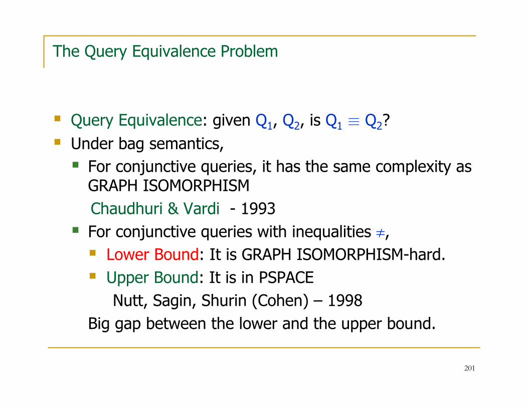
201
The Query Equivalence Problem
� Query Equivalence: given Q1, Q2, is Q1 ≡ Q2?
� Under bag semantics,
� For conjunctive queries, it has the same complexity as GRAPH ISOMORPHISM
Chaudhuri & Vardi - 1993
� For conjunctive queries with inequalities g,
� Lower Bound: It is GRAPH ISOMORPHISM-hard.
� Upper Bound: It is in PSPACE
Nutt, Sagin, Shurin (Cohen) – 1998
Big gap between the lower and the upper bound.

202
Limitations of Relational Algebra & Relational Calculus
Outline:
� Relational Algebra and Relational Calculus have substantial expressive power. In particular, they can express
� Natural Join
� Quotient
� Unions of conjunctive queries
� …
� However, they cannot express recursive queries.
� Datalog is a declarative database query language that augments the language of conjunctive queries with a recursion mechanism.

203
Parents, Grandparents, and Greatgrandparents
� Let PARENT be a binary relational schema such that if
(a,b) ∈ PARENT in some database instance, then a is a parent of b.
� Using PARENT, we can define GRANDPARENT and GREATGRANPARENT by the conjunctive queries:
GRANDPARENT(x,y) :- PARENT(x,z), PARENT(z,y)
and
GREATGRANDPARENT(x,y) :- PARENT(x,z), PARENT(z,w),
PARENT(w,y)
� Similarly, we can define GREATGREATGRANPARENT by a conjunctive query, and so on up to any fixed level of ancenstry.

204
Parents and Ancestors
� Question: Is there a relational algebra (relational calculus) expression that defines ANCESTOR from PARENT?
� Note: This type of question occurs in other related concepts:
� Given a binary relation MANAGES(manager, employee), is there a relational algebra (relational calculus) expression that definesHIGHER-MANAGER
� Given a binary relation DIRECT(from,to) about flights, is there a relational algebra (relational calculus) expression that definesCAN-FLY(from,to)?
� More abstractly, given a binary relation E, is there a relational algebra (relational calculus) expression that defines the Transitive Closure TC of E?
205
Edges and Paths
Definition: Let E be a binary relation
� For every n ≥ 1, let PATHn be the binary query:
“given a and b, is there a path of length n from a to b along edges from E?”
� PATH is the binary query:
“given a and b, is there a path from a to b along edges from E?”
Fact:
� For every n≥ 1, the query PATHn is expressible by a conjunctive query. (Why?)
� Hence, PATH is expressible by an infinite union of conjunctive queries:
PATH ≡ PATH1 ∪ PATH2 ∪ … ∪ PATHn ∪ …

206
Edges, Paths, and Transitive Closure
Facts: Let E be a binary relation
� PATH is the Transitive Closure of E, i.e.,
the smallest binary relation T such that
� E ⊆ T
� T is transitive (if (a,b) ∈ T and (b,c) ∈ T, then (a,c) ∈ T).
� There are several well-known efficient algorithms for computing the Transitive Closure of a given binary relation E
� Floyd–Warshall Algorithm (taught in CMPS 101).
� Recall that the following problem is NLOGSPACE-complete:
Given E, a and b, is there a path from a to b? (i.e., is (a,b) ∈ TC?)

207
Transitive Closure and Relational Calculus
� Question: Is there a relational algebra (relational calculus) expression that defines ANCESTOR from PARENT? In other words, is there a relational algebra (relational calculus) expression that defines the Transitive Closure of a given binary relation E?
� Theorem: A. Aho and J. Ullman – 1979
There is no relational algebra (or relational calculus) expression that defines the Transitive Closure of a given binary relation E.
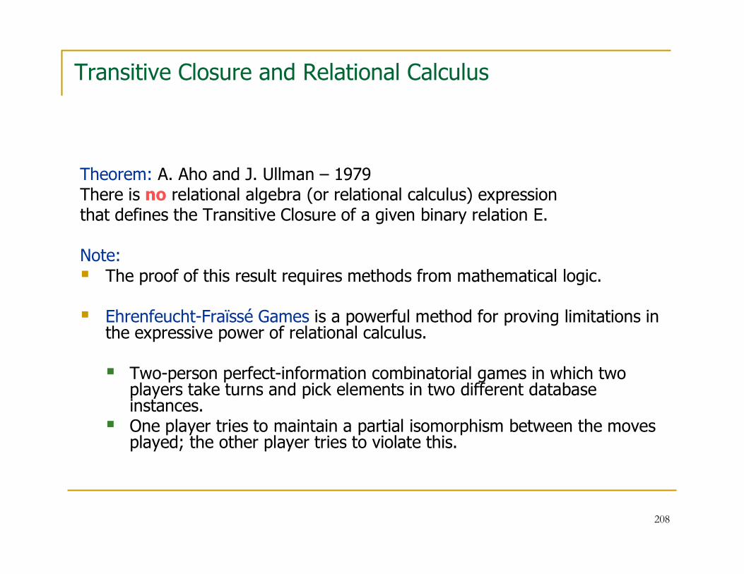
208
Transitive Closure and Relational Calculus
Theorem: A. Aho and J. Ullman – 1979There is no relational algebra (or relational calculus) expressionthat defines the Transitive Closure of a given binary relation E.
Note: � The proof of this result requires methods from mathematical logic.
� Ehrenfeucht-Fraïssé Games is a powerful method for proving limitations in the expressive power of relational calculus.
� Two-person perfect-information combinatorial games in which two players take turns and pick elements in two different database instances.
� One player tries to maintain a partial isomorphism between the moves played; the other player tries to violate this.

209
Transitive Closure and Relational Calculus
Theorem: A. Aho and J. Ullman – 1979
There is no relational algebra (or relational calculus) expression
that defines the Transitive Closure of a given binary relation E.
Intuition behind this result:
� Relational Calculus queries can only express “local” properties
E Ft
s
t
s

210
Limitations of Relational Calculus and Relational Calculus
� There is no relational algebra (relational calculus) expression involving PARENT that defines ANCESTOR.
� ANCESTOR is definable by an infinite union of conjunctive queries, but is not definable by any finite union of conjunctive queries.
� Aho and Ullman’s Theorem reveals a limitation in the expressive power of relational algebra and relational calculus, namely
� They cannot express recursive queries.

211
Overcoming the Limitations of Relational Calculus
� Question: What is to be done to overcome the limitations of the expressive power of relational calculus?
� Answer 1: Embedded Relational Calculus (Embedded SQL):
� Allow SQL commands inside a conventional programming language, such as C, Java, etc.
� This is an inferior solution, as it destroys the high-level character of SQL.
� Answer 2:
� Augment relational calculus with a high-level declarative mechanism for recursion.
� Conceptually, this a superior solution as it maintains the high-level declarative character of relational calculus.

212
Datalog
� Datalog = “Conjunctive Queries + Recursion”
� Datalog was introduced by Chandra and Harel in 1982 and has been studied by the research community in depth since that time:
� Hundreds of research papers in major database conferences;
� Numerous doctoral dissertations.
� Recent applications outside databases:
� Specification of network properties
� Access control languages
� SQL:1999 and subsequent versions of the SQL standard provide support for a sublanguage of Datalog, called linear Datalog.

213
Datalog Syntax
� Definition: A Datalog program π is a finite set of rules each expressing a conjunctive query
T(x1,…,xk) :-- R1(u1), …, Rn(un),
where each variable xi occurs in the body of the rule.
� Some relational symbols occurring in the heads of the rules may
also occur in the bodies of the rules
(unlike the rules for conjunctive queries).
� These relational symbols are the recursive relational symbols; they are also known as intensional database predicates (IDBs).
� The remaining relational symbols in the rules are known as the extensional database predicates (EDBs).

214
Datalog
� Example: Datalog program for Transitive Closure
T(x,y) :- E(x,y)
T(x,y) :- E(x,z), T(z,y)
� E is the EDB predicate
� T is the IDB predicate
� The intuition is that the Datalog program gives a recursive specification of the IDB predicate T in terms of the EDB E.
� Example: Another Datalog program for Transitive Closure
T(x,y) :- E(x,y)
T(x,y) :- T(x,z), T(z,y)
(“divide and conquer” algorithm for Transitive Closure)
215
Datalog
� Example: Paths of Even and Odd Length
Consider the Datalog program:
ODD(x,y) :- E(x,y)
ODD(x,y) :- E(x,z), EVEN(z,y)
EVEN(x,y) :- E(x,z), ODD(z,y).
� E is the EDB predicate
� EVEN and ODD are the IDB predicates.
� So, a Datalog program may have several different IDB predicates (and it may have several different EDB predicates as well).
� This program gives a recursive specification of the IDB predicates EVEN and ODD in terms of the EDB predicate E.
� This is a Datalog program expressing mutual recursion.

216
Conjunctive Queries vs. Datalog
� As we have seen, conjunctive queries can be written as rules:
T(x1,…,xk) :-- R1(u1), …, Rn(un).
� In such a rule, the relation symbol in the head does not occurin the body of the rule.
� Datalog programs are finite sets of rules.
� In a Datalog program, however, a relation symbols occurring in the heads of a rule:
� may also occur in the body of the same rule
T(x,y) :- E(x,z), T(z,y)
� or, it may occur in the body of another rule in the program
ODD(x,y) :- E(x,z), EVEN(z,y)
EVEN(x,y) :- E(x,z), ODD(z,y).

217
Datalog Semantics
� Question: What is the precise semantics of a Datalog program?
� Answer: Datalog programs can be given two different types of semantics.
� Declarative Semantics (denotational semantics)
� Smallest solutions of recursive specifications.
� Least fixed-points of monotone operators.
� Procedural Semantics (operational semantics)
� An iterative process for computing the “meaning” of Datalogprograms.
� Main Result: The declarative semantics coincides with the procedural semantics.
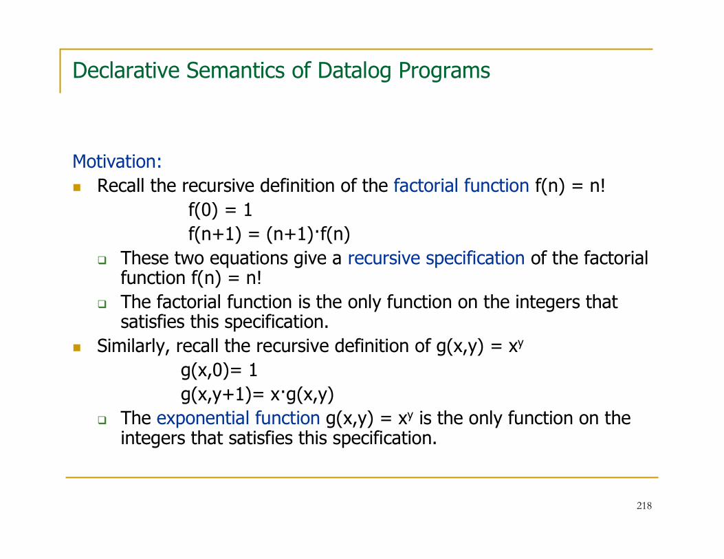
218
Declarative Semantics of Datalog Programs
Motivation:
� Recall the recursive definition of the factorial function f(n) = n!
f(0) = 1
f(n+1) = (n+1)�f(n)
� These two equations give a recursive specification of the factorial function f(n) = n!
� The factorial function is the only function on the integers thatsatisfies this specification.
� Similarly, recall the recursive definition of g(x,y) = xy
g(x,0)= 1
g(x,y+1)= x�g(x,y)
� The exponential function g(x,y) = xy is the only function on the integers that satisfies this specification.

219
Declarative Semantics of Datalog Programs
� Each Datalog program can be viewed as a recursive specification of its IDB predicates.
� This specification is expressed using relational algebra operators
� The body of each rule uses π, σ, and cartesian product ×
� All rules having the same predicate in the head are combined using union.
� The recursive specification is given by equations involving
unions of conjunctive queries.
� Example: T(x,y) :- E(x,y)
T(x,y):- T(x,z), T(z,y)
� Recursive equation:
T = E ∪ π1,4(σ$2=$3 (T×T))
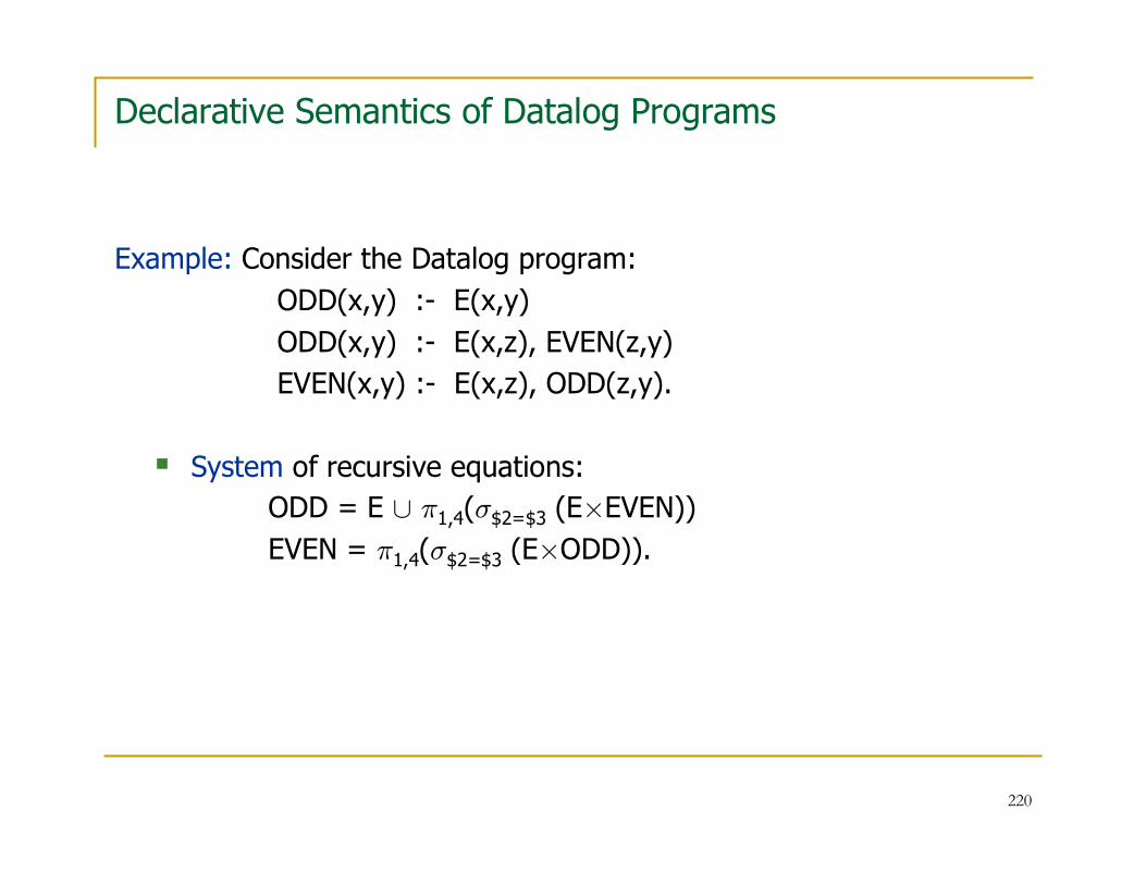
220
Declarative Semantics of Datalog Programs
Example: Consider the Datalog program:
ODD(x,y) :- E(x,y)
ODD(x,y) :- E(x,z), EVEN(z,y)
EVEN(x,y) :- E(x,z), ODD(z,y).
� System of recursive equations:
ODD = E ∪ π1,4(σ$2=$3 (E×EVEN))
EVEN = π1,4(σ$2=$3 (E×ODD)).

221
Declarative Semantics of Datalog Programs
� Unlike the recursive equations for the factorial and the exponential
function, recursive equations arising from Datalog programs
need not have a unique solution.
� Example: Consider the recursive equation:
T = E ∪ π1,4(σ$2=$3 (T×T))
Let E = { (1,2), (2,3) }.
Then both T1 and T2 satisfy this recursive equation, where
� T1 = { (1,2), (2,3), (1,3) }
� T2 = { (1,2),(2,1),(2,3),(3,2),(1,3),(3,2),(1,1),(2,2),(3,3) }.
Furthermore, this recursive equation has many other solutions.
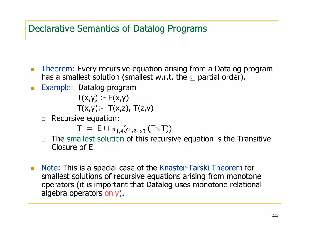
222
Declarative Semantics of Datalog Programs
� Theorem: Every recursive equation arising from a Datalog program has a smallest solution (smallest w.r.t. the ⊆ partial order).
� Example: Datalog program
T(x,y) :- E(x,y)
T(x,y):- T(x,z), T(z,y)
� Recursive equation:
T = E ∪ π1,4(σ$2=$3 (T×T))
� The smallest solution of this recursive equation is the Transitive Closure of E.
� Note: This is a special case of the Knaster-Tarski Theorem for smallest solutions of recursive equations arising from monotone operators (it is important that Datalog uses monotone relational algebra operators only).

223
Declarative Semantics of Datalog Programs
� Theorem: Every recursive equation arising from a Datalog program has a smallest solution (smallest w.r.t. the ⊆ partial order).
� Definition: The (declarative) semantics of a Datalog program is the smallest solution of the system of recursive equations arising from the Datalog program.
� Note:
� If the Datalog program has more than one IDBs, then we get a system of recursive equations, instead of single one.
� Question:
� What does “smallest solution of a system” mean in this case?
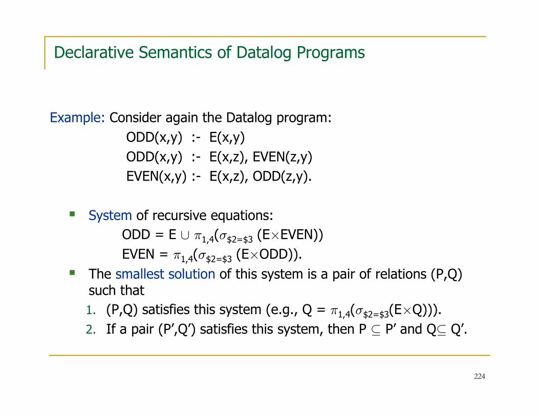
224
Declarative Semantics of Datalog Programs
Example: Consider again the Datalog program:
ODD(x,y) :- E(x,y)
ODD(x,y) :- E(x,z), EVEN(z,y)
EVEN(x,y) :- E(x,z), ODD(z,y).
� System of recursive equations:
ODD = E ∪ π1,4(σ$2=$3 (E×EVEN))
EVEN = π1,4(σ$2=$3 (E×ODD)).
� The smallest solution of this system is a pair of relations (P,Q) such that
1. (P,Q) satisfies this system (e.g., Q = π1,4(σ$2=$3(E×Q))).
2. If a pair (P’,Q’) satisfies this system, then P ⊆ P’ and Q⊆ Q’.

225
Declarative Semantics of Datalog Programs
� Question:
� How difficult is it to compute the declarative semantics of Datalog programs?
� In other words, what is the computational complexity of the query evaluation problem for Datalog queries?
� Note: On the face of their definition, the declarative semantics of Datalog programs do not give rise to an algorithm for computing this semantics.

226
Procedural Semantics of Datalog Programs
Definition: Let π be a Datalog program. The procedural semantics of π
are obtained by the following bottom-up evaluation of the recursive
predicates (IDBs) of π:
1. Set all IDBs of π to ∅.
2. Apply all rules of π in parallel; update the IDBs by evaluating the bodies of the rules.
3. Repeat until no IDB predicate changes.
4. Return the values of the IDB predicates obtained at the end of Step 3.

227
Procedural Semantics of Datalog Programs
Example: Datalog program for Transitive Closure
T(x,y) :- E(x,y)
T(x,y):- E(x,z),T(z,y)
� Bottom-up evaluation:
T0 = ∅
Tn+1 = {(a,b): E(a,b) Ç ∃ z(E(a,z) Æ Tn(z,b))}
Fact: The following statements are true:
� Tn ={ (a,b): there is a path of length at most n from a to b }
� Transitive Closure of E = ∪ n ≥ 1Tn.
Proof: By induction on n.

228
Procedural Semantics of Datalog Programs
Example: Another Datalog program for Transitive Closure
T(x,y) :- E(x,y)
T(x,y):- T(x,z),T(z,y)
� Bottom-up evaluation:
T0 = ∅
Tn+1 = {(a,b): E(a,b) Ç ∃ z(Tn(a,z) Æ Tn(z,b))}
Fact: The following statements are true:
� Tn ={ (a,b): there is a path of length at most 2n from a to b }
� Transitive Closure of E = ∪ n ≥ 1Tn.
Proof: By induction on n.

229
Procedural Semantics of Datalog Programs
Example: Consider the Datalog program ODD(x,y) :- E(x,y)ODD(x,y) :- E(x,z), EVEN(z,y)EVEN(x,y) :- E(x,z), ODD(z,y)
� Bottom-up evaluation:ODD0 = ∅EVEN0 = ∅ODDn+1 = {(a,b): E(a,b) Ç ∃ z(E(a,z) Æ EVENn(z,b))}EVENn+1 = {(a,b): ∃ z(E(a,z) Æ ODDn(z,b))}
Fact: The following statements are true:� ∪ n ≥ 1 ODDn = { (a,b): there is a path of odd length from a to b }� ∪ n ≥ 1 EVENn = { (a,b): there is a path of even length from a to b }.
Proof: By induction on n.

230
Declarative vs. Procedural Datalog Semantics
Theorem: Let π be a Datalog program. Then the following are true:
� The bottom-up evaluation of the procedural semantics of πterminates within a number of steps bounded by a polynomial in the size of the database instance (= size of the EDB predicates).
� The declarative semantics of π coincides with the procedural semantics of π.
Proof: For simplicity, assume that π has a single IDB T of arity k.
� By induction on n, show that Tn ⊆ Tn+1, for every n.
(this uses the monotonicity of unions of conjunctive queries).
� Hence, T0 ⊆ T1 ⊆ … ⊆ Tn ⊆ Tn+1 ⊆ …
� Since each Tn ⊆ adom(I)k, there is an m ≤ |adom(I)|k such that Tm = Tm+1.

231
Declarative vs. Procedural Datalog Semantics
Theorem: Let π be a Datalog program. Then the following are true:
� The bottom-up evaluation of the procedural semantics of πterminates within a number of steps bounded by a polynomial in the size of the database instance (= size of the EDB predicates).
� The declarative semantics of π coincides with the procedural semantics of π.
Proof: For simplicity, assume that π has a single IDB T of arity k.
� Since Tm = Tm+1, we have that the procedural semantics produces a solution to the recursive equation arising from π.
� By induction on n, show that if T* is another solution of this recursive equation, then Tn ⊆ T*, for all n
(use the monotonicity of unions of conjunctive queries again).
� In particular, Tm ⊆ T*, hence Tm is the smallest solution of this recursive equation.

232
The Query Evaluation Problem for Datalog
Theorem: Let π be a Datalog program. There is a polynomial-time
algorithm such that, given a database instance I, it evaluates π on I
(i.e., it computes the semantics of π on I).
Proof: The bottom-up evaluation of the procedural semantics of π runs
in polynomial time because:
� The number of iterations is bounded by a polynomial in the size of I.
� Each step of the iteration can be carried out in polynomial time
(why?).
Corollary: The data complexity of Datalog is in P.

233
The Query Evaluation Problem for Datalog
Corollary: The data complexity of Datalog is in P.
Theorem: The combined complexity of Datalog is EXPTIME-complete.
Note:
� P ⊆ NP ⊆ PSPACE ⊆ EXPTIME.
� Moreover, it is known that P is properly contained in EXPTIME.
� Thus, Datalog has higher combined complexity than relational calculus (since the combined complexity of relational calculus is PSPACE-complete).

234
Some Interesting Datalog Programs
Example: Non 2-Colorability can be expressed by a Datalog program.
Fact: A graph E is 2-colorable if and only if it does not contain a cycle
of odd length.
Datalog program for Non 2-Colorability:
ODD(x,y) :-- E(x,y)
ODD(x,y) :-- E(x,z), EVEN(z,y)
EVEN(x,y) :-- E(x,z), ODD(z,y).
Q :-- ODD(x,x)
Sanity check: Can you find a Datalog program for Non 3-Colorability?

235
Some Interesting Datalog Programs
Example: Path Systems Problem
T(x) :-- A(x)
T(x) :-- R(x,y,z), T(y), T(z)
Theorem: S. Cook – 1974
Evaluating this Datalog program is a P-complete problem
(via logspace-reductions).
Note:
� Path Systems was the first problem shown to be P-complete.
� In particular, it is highly unlikely that Path Systems is in NLOGSPACE or in LOGSPACE.
� In this sense, Datalog has higher data complexity than relational calculus.

236
Procedural Semantics of Datalog Programs
� On the face of it, the bottom-up evaluation of Datalog programs is an infinite process, since it gives rise to an infinite sequence of “stages” T0, T1, …,Tn, …
� Question: Does this infinite sequence converge?
� It will turn out that, for every Datalog program π and for every database instance I, the bottom-up evaluation of π on I terminates within a number of steps that is bounded by some polynomial in the size of I, i.e., there is some m such that
Tm = Tm+1.
Moreover, the smallest such m is bounded by some polynomial in the size of I.

237
Declarative vs. Procedural Datalog Semantics
Theorem: Let π be a Datalog program. Then the following are true:
� On every database instance I, the bottom-up evaluation of the procedural semantics of π terminates within a number of steps bounded by a polynomial in the size of I.
� The declarative semantics of π coincides with the procedural semantics of π.
Proof: For simplicity, assume that π has a single IDB T of arity k.
� By induction on n, show that Tn ⊆ Tn+1, for every n.
(this uses the monotonicity of unions of conjunctive queries).
� Hence, T0 ⊆ T1 ⊆ … ⊆ Tn ⊆ Tn+1 ⊆ …
� Since each Tn ⊆ adom(I)k, there is an m ≤ |adom(I)|k such that Tm = Tm+1.

238
Declarative vs. Procedural Datalog Semantics
Theorem: Let π be a Datalog program. Then the following are true:
� The bottom-up evaluation of the procedural semantics of πterminates within a number of steps bounded by a polynomial in the size of the database instance (= size of the EDB predicates).
� The declarative semantics of π coincides with the procedural semantics of π.
Proof: For simplicity, assume that π has a single IDB T of arity k.
� Since Tm = Tm+1, we have that the procedural semantics produces a solution to the recursive equation arising from π.
� By induction on n, show that if T* is another solution of this recursive equation, then Tn ⊆ T*, for all n
(use the monotonicity of unions of conjunctive queries again).
� In particular, Tm ⊆ T*, hence Tm is the smallest solution of this recursive equation.

239
The Query Evaluation Problem for Datalog
Theorem: Let π be a Datalog program. There is a polynomial-time
algorithm such that, given a database instance I, it evaluates π on I
(i.e., it computes the semantics of π on I).
Proof: The bottom-up evaluation of the procedural semantics of π runs
in polynomial time because:
� The number of iterations is bounded by a polynomial in the size of I.
� Each step of the iteration can be carried out in polynomial time
(why?).
Corollary: The data complexity of Datalog is in P.

240
The Query Evaluation Problem for Datalog
Corollary: The data complexity of Datalog is in P.
Theorem: The combined complexity of Datalog is EXPTIME-complete.
Note:
� P ⊆ NP ⊆ PSPACE ⊆ EXPTIME.
� Moreover, it is known that P is properly contained in EXPTIME.
� Thus, Datalog has higher combined complexity than relational calculus (since the combined complexity of relational calculus is PSPACE-complete).

241
Some Interesting Datalog Programs
Example: Non 2-Colorability can be expressed by a Datalog program.
Fact: A graph E is 2-colorable if and only if it does not contain a cycle
of odd length.
Datalog program for Non 2-Colorability:
ODD(x,y) :-- E(x,y)
ODD(x,y) :-- E(x,z), EVEN(z,y)
EVEN(x,y) :-- E(x,z), ODD(z,y).
Q :-- ODD(x,x)
Sanity check: Can you find a Datalog program for Non 3-Colorability?

242
Some Interesting Datalog Programs
Example: Path Systems Problem
T(x) :- A(x)
T(x) :- R(x,y,z), T(y), T(z)
Theorem: S. Cook – 1974
Evaluating this Datalog program is a P-complete problem
(via logspace-reductions).
Note:
� Path Systems was the first problem shown to be P-complete.
� In particular, it is highly unlikely that Path Systems is in NLOGSPACE or in LOGSPACE.
� In this sense, Datalog has higher data complexity than relational calculus.

243
Linear Datalog
� Definition: A Datalog program is linear if the body of each rule contains at most one atomic formula involving an IDB predicate.
� Example: Linear Datalog Program for Transitive Closure
T(x,y) :- E(x,y)
T(x,y) :- E(x,z), T(z,y)
� Example: Non-linear Datalog program for Transitive Closure
T(x,y) :- E(x,y)
T(x,y) :- T(x,z), T(z,y)

244
Linear Datalog
Example: Give a linear Datalog program that computes the binary query COUSIN from the binary relation schema PARENT
SIBLING(x,y) :- PARENT(z,x), PARENT(z,y)COUSIN(x,y) :- PARENT(z,x), PARENT(w,y), SIBLING(z,w)COUSIN(x,y) :- PARENT(z,x), PARENT(w,y), COUSIN(z,w).
Fact: COUSIN(Barack Obama, Dick Chenney) Actually, COUSIN8(Barack Obama, Dick Chenney)
http://www.msnbc.msn.com/id/21340764/
Fact: COUSIN(Sarah Palin, Princess Diana). Actually, COUSIN10(Sarah Palin, Princess Diana)
http://www.dailymail.co.uk/news/worldnews/article-1073249/Sarah-Palin-Princess-Diana-cousins-genealogists-reveal.html

245
Linear Datalog
� Definition: A Datalog program π is linearizable if there is a linear Datalog program π* that is equivalent to π.
� Example: The following Datalog program is linearizable:
T(x,y) :- E(x,y)
T(x,y) :- T(x,z), T(z,y)
� Example: The following Datalog program is not linearizable:
T(x) :- A(x)
T(x) :- R(x,y,z), T(y), T(z)
(the proof of this fact is non-trivial).

246
Datalog and SQL
� SQL:99 and subsequent versions of the SQL standard provide support for linear Datalog programs (but not for non-linear ones)
� Syntax:
WITH RECURSIVE T AS
<Datalog program for T>
<query involving T>
� Semantics:
� Compute T as the semantics of <Datalog program for T>
� The result of the previous step is a temporary relation that is then used, together with other EDBS, as if it were a stored relation (an EDB) in <query involving T>.
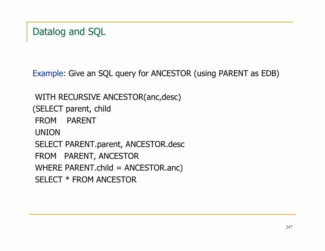
247
Datalog and SQL
Example: Give an SQL query for ANCESTOR (using PARENT as EDB)
WITH RECURSIVE ANCESTOR(anc,desc)
(SELECT parent, child
FROM PARENT
UNION
SELECT PARENT.parent, ANCESTOR.desc
FROM PARENT, ANCESTOR
WHERE PARENT.child = ANCESTOR.anc)
SELECT * FROM ANCESTOR

248
Datalog and SQL
Example: Give an SQL query that computes all descendants of Noah
WITH RECURSIVE ANCESTOR(anc,desc)
(SELECT parent, child
FROM PARENT
UNION
SELECT ANCESTOR.anc, PARENT.child
FROM PARENT, ANCESTOR
WHERE PARENT.child = ANCESTOR.anc)
SELECT desc FROM ANCESTOR
WHERE anc = ‘Noah’

249
Datalog and SQL
� Linear Datalog programs with mutiple IDBs are supported in SQL:99
� Syntax:
WITH RECURSIVE R, S, T, … AS
<Datalog program for R, S, T, …>
<query involving R, S, T, … >
� Semantics:
� Compute R, S, T, … as the semantics of
<Datalog program for R, S, T, …>
� The result of the previous step are temporary relation that are then used, together with other EDBS, as if they were stored relation (EDBs) in <query involving R, S, T, …>.

250
Datalog(≠)
� Definition: Datalog(≠)
� Datalog(≠) is the extension of Datalog in which the body of a rule may contain also ≠.
� Declarative and Procedural Semantics of Datalog(≠) are similar to those of Datalog.
� Example: w-AVOIDING PATH
Given a graph E and three nodes x,y, and w, is there a path from x to y that does not contain w?
T(x,y,w) :- E(x,y), x ≠ w, y ≠ w
T(x,y,w) :- E(x,z), T(z,y,w), x ≠ w.

251
Datalog with Negation
� Question: What if we allow negation in the bodies of Datalog rules?
� Examples:
� T(x) :- ¬ T(x)
(the recursive specification has no solutions!)
� S(x) :- E(x,y), ¬ S(y)
� Note: Several different semantics for Datalog programs with negation have been proposed over the years (see Ch. 15 of AHV):
� Stratified datalog programs
� Well-founded semantics
� Inflationary semantics
� Stable model semantics
� …

252
Query Equivalence and Containment for Datalog
� Note: Recall that the following are known about the Query Evaluation Problem for Datalog queries:
� The data complexity of Datalog is in P.
� The combined complexity of Datalog is EXPTIME-complete.
� Questions:
� What about the Query Equivalence Problem for Datalog:
Given two Datalog programs π and π’, is π equivalent to π’?
(do they return the same answer on every database instance?)
� What about the Query Containment Problem for Datalog:
Given two Datalog programs π and π’, is π ⊆ π’?
(is π(I) ⊆ π’(I), on every database instance I?)

253
Query Equivalence and Containment for Datalog
Theorem: O. Shmueli – 1987
� The query equivalence problem for Datalog queries is undecidable. In fact, it is undecidable even for Datalog queries with a single IDB.
� Consequently, the query containment problem for Datalog queries is undecidable.
Hint of Proof:
� Reduction from Context-Free Grammar Equivalence:
Given two context-free grammars G and G’, is L(G) = L(G’)?
For more on this topic, read Chapter 12 of AHV.

254
The Complexity of Database Query Language
UndecidableNP-completeNP-completeUndecidableQuery Containment
UndecidableNP-completeNP-completeUndecidableQuery Equivalence
P-completeIn LOGSPACE (hence, in P)
In LOGSPACE (hence, in P)
In LOGSPACE (hence, in P)
Query Eval.:
Data Complexity
EXPTIME-complete
NP-completeNP-completePSPACE-complete
Query Eval.: Combined Complexity
Datalog
Queries
Unions of Conjunctive Queries
Conjunctive Queries
Relational Calculus

Composing Schema Mappings:An Overview
� This topic complements the topics on data integration and data exchange presented in the course by Maurizio Lenzerini.
� It is joint work with Ronald Fagin, Lucian Popa, and Wang-Chiew Tan.

256
Theoretical Aspects of Data Interoperability
The research community has studied two different, but
closely related, facets of data interoperability:
� Data Integration (aka Data Federation)
� Formalized and studied for the past 10-15 years
� Data Exchange (aka Data Translation)
� Formalized and studied for the past 5-6 years

257
Data Integration
Query heterogeneous data in different sources via a virtual
global schema
I1
Global
SchemaI2
I3 Sources
query
S1
S2
S3
T
Q

258
Data Exchange
Transform data structured under a source schema into data structured under a different target schema.
S T
Σ
IJ
Source Schema Target Schema
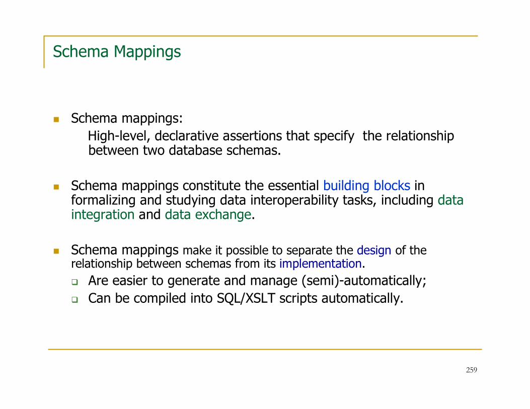
259
Schema Mappings
� Schema mappings:
High-level, declarative assertions that specify the relationship between two database schemas.
� Schema mappings constitute the essential building blocks in formalizing and studying data interoperability tasks, including data integration and data exchange.
� Schema mappings make it possible to separate the design of the relationship between schemas from its implementation.
� Are easier to generate and manage (semi)-automatically;
� Can be compiled into SQL/XSLT scripts automatically.
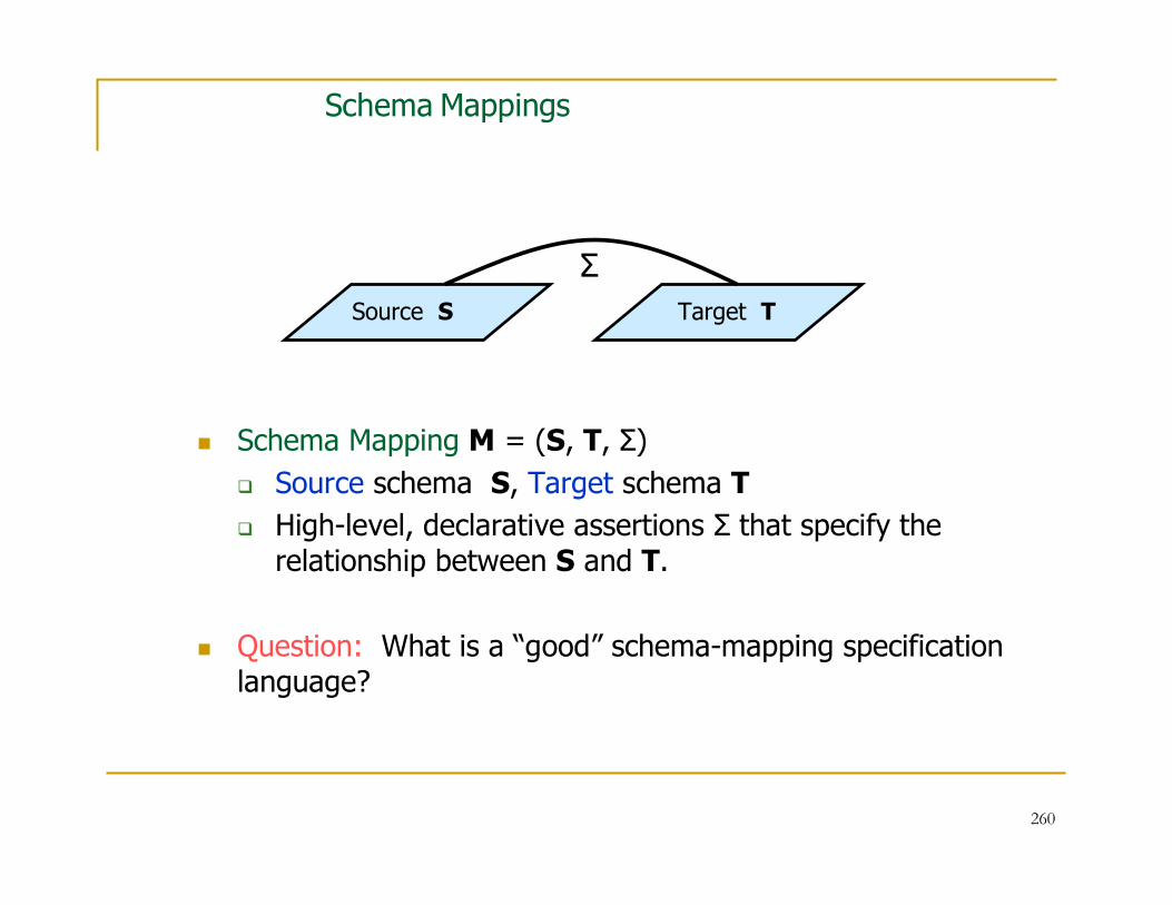
260
Schema Mappings
Source S Target T
� Schema Mapping M = (S, T, Σ)
� Source schema S, Target schema T
� High-level, declarative assertions Σ that specify the relationship between S and T.
� Question: What is a “good” schema-mapping specification language?
Σ

261
Schema-Mapping Specification Languages
� Obvious Idea:
Use a logic-based language to specify schema mappings.
In particular, use first-order logic.
� Warning:
Unrestricted use of first-order logic as a schema-mapping specification language gives rise to undecidability of basic algorithmic problems about schema mappings.

262
Schema Mapping Specification Languages
Let us consider some simple tasks that every schema-mapping specification
language should support:
� Copy (Nicknaming):
� Copy each source table to a target table and rename it.
� Projection:
� Form a target table by projecting on one or more columns of a source table.
� Column Augmentation:
� Form a target table by adding one or more columns to a source table.
� Decomposition:
� Decompose a source table into two or more target tables.
� Join:
� Form a target table by joining two or more source tables.
� Combinations of the above (e.g., “join + column augmentation + …”)

263
Schema Mapping Specification Languages
� Copy (Nicknaming):
� ∀x1, …,xn(P(x1,…,xn) → R(x1,…,xn))
� Projection:
� ∀x,y,z(P(x,y,z) → R(x,y))
� Column Augmentation:
� ∀x,y (P(x,y) → ∃ z R(x,y,z))
� Decomposition:
� ∀x,y,z (P(x,y,z) → R(x,y)Æ T(y,z))
� Join:
� ∀x,y,z(E(x,z)ÆF(z,y) → R(x,y,z))
� Combinations of the above (e.g., “join + column augmentation + …”)
� ∀x,y,z(E(x,z)Æ F(z,y) → ∃ w (R(x,y) Æ T(x,y,z,w)))

264
Schema Mapping Specification Languages
� Question: What do all these tasks (copy, projection, column augmentation, decomposition, join) have in common?
� Answer:
� They can be specified using
tuple-generating dependencies (tgds).
� In fact, they can be specified using a special class of
tuple-generating dependencies known as
source-to-target tuple generating dependencies (s-t tgds).

265
Database Integrity Constraints
� Dependency Theory: extensive study of integrity constraints in relational databases in the 1970s and 1980s
(Codd, Fagin, Beeri, Vardi …)
� Tuple-generating dependencies (tgds) emerged as an important class of constraints with a balance between high expressive power and good algorithmic properties. Tgds are expressions of the form
∀ x (ϕ(x) → ∃ y ψ(x, y )), where
ϕ(x), ψ(x, y ) are conjunctions of atomic formulas.
Special Cases:
� Inclusion Dependencies
� Multivalued Dependencies

266
Schema Mapping Specification Language
The relationship between source and target is given by
source-to-target tuple generating dependencies (s-t tgds)
∀x (ϕ(x) → ∃y ψ(x, y)), where
� ϕ(x) is a conjunction of atoms over the source;
� ψ(x, y) is a conjunction of atoms over the target.
� s-t tgds assert that: some conjunctive query over the source is contained in some other conjunctive query over the target.
Example: (dropping the universal quantifiers in the front)
(Student (s) ∧ Enrolls(s,c)) → ∃t ∃g (Teaches(t,c) ∧ Grade(s,c,g))

267
Schema Mapping Specification Language
Fact: s-t tgds generalize the main specifications used in data integration:
� They generalize LAV (local-as-view) specifications:
P(x) → ∃y ψ(x, y), where P is a source schema.
� E(x,y) → ∃ z (H(x,z)Æ H(z,y)) (LAV constraint)
Note: Copy, projection, and decomposition are LAV s-t tgds.
� They generalize GAV (global-as-view) specifications:
ϕ(x) → R(x), where R is a target relation
(they are equivalent to full tgds: ϕ(x) → ψ(x),
where ϕ(x) and ψ(x) are conjunctions of atoms).
� E(x,y) Æ E(y,z) → F(x,z) (GAV (full) constraint)
Note: Copy, projection, and join are GAV s-t tgds.

268
Schema Mappings & Data Exchange
Source S Target T
� Data Exchange via the schema mapping M = (S, T, Σ)
Given a source instance I, construct a target instance J, so that (I, J) satisfy the specifications Σ of M.
Such a J is called a solution for I.
� Difficulty:
� Usually, there are multiple solutions
� Which one is the “best” to materialize?
IJ
Σ

269
Data Exchange & Universal solutions
Fagin, K …, Miller, Popa:
Identified and studied the concept of a universal solution for
schema mappings specified by s-t tgds
� A universal solutions is a most general solution.
� A universal solution “represents” the entire space of solutions.
� A “canonical” universal solution can be generated efficiently using the chase procedure.
� A universal solution can be used to compute the certain answers of conjunctive queries over the target schema.

270
Managing Schema Mappings
� Schema mappings can be quite complex.
� Methods and tools are needed to automate or semi-automate schema-mapping management.
� Metadata Management Framework – Bernstein 2003
based on generic schema-mapping operators:
� Match operator
� Merge operator
� …
� Composition operator
� Inverse operator

271
Composing Schema Mappings
� Given M12 = (S1, S2, Σ12) and M23 = (S2, S3, Σ23), derive a
schema mapping M13 = (S1, S3, Σ13) that is “equivalent” to the
sequential application of M12 and M23.
� M13 is a composition of M12 and M23
M13 = M12 ◦ M23
Schema S1 Schema S2 Schema S3
M12 M23
M13
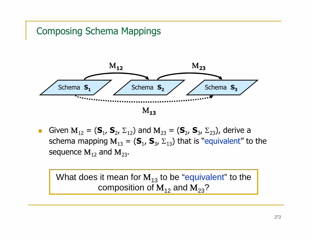
272
Composing Schema Mappings
� Given ΜΜΜΜ12 = (S1, S2, Σ12) and ΜΜΜΜ23 = (S2, S3, Σ23), derive a
schema mapping ΜΜΜΜ13 = (S1, S3, Σ13) that is “equivalent” to the
sequence ΜΜΜΜ12 and ΜΜΜΜ23.
Schema S1 Schema S2 Schema S3
ΜΜΜΜ12 ΜΜΜΜ23
ΜΜΜΜ13
What does it mean for ΜΜΜΜ13 to be “equivalent” to the composition of ΜΜΜΜ12 and ΜΜΜΜ23?
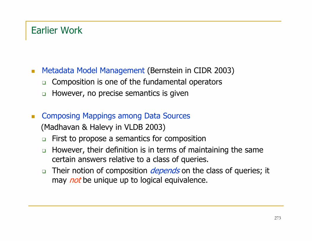
273
Earlier Work
� Metadata Model Management (Bernstein in CIDR 2003)
� Composition is one of the fundamental operators
� However, no precise semantics is given
� Composing Mappings among Data Sources
(Madhavan & Halevy in VLDB 2003)
� First to propose a semantics for composition
� However, their definition is in terms of maintaining the same certain answers relative to a class of queries.
� Their notion of composition depends on the class of queries; it may not be unique up to logical equivalence.

274
Semantics of Composition
� Every schema mapping M = (S, T, Σ) defines a binary relationship Inst(M) between
instances:
Inst(M) = { (I,J) | (I,J) ~ Σ }.
In fact, from a semantic point of view, a schema mapping M can be
identified with the set Inst(M).
� Definition: (FKPT)
A schema mapping M13 is a composition of M12 and M23 if
Inst(M13) = Inst(M12) ° Inst(M23), that is,
(I1,I3) ~ Σ13
if and only if
there exists I2 such that (I1,I2) ~ Σ12 and (I2,I3) ~ Σ23.

275
The Composition of Schema Mappings
Fact: If both ΜΜΜΜ = (S1, S3, Σ) and ΜΜΜΜ’ = (S1, S3, Σ’) are
compositions of ΜΜΜΜ12 and ΜΜΜΜ23, then Σ are Σ’ are logically equivalent.
For this reason:
� We say that ΜΜΜΜ (or ΜΜΜΜ’) is the composition of ΜΜΜΜ12 and ΜΜΜΜ23.
� We write ΜΜΜΜ12 ° ΜΜΜΜ23 to denote it

276
Issues in Composition of Schema Mappings
� The semantics of composition was the first main issue.
� The second main issue is the language of the composition.
� Is the language of s-t tgds closed under composition?
If ΜΜΜΜ12 and ΜΜΜΜ23 are specified by finite sets of s-t tgds, is
ΜΜΜΜ12 ° ΜΜΜΜ23 also specified by a finite set of s-t tgds?
� If not, what is the “right” language for composing schema mappings?

277
Inexpressibility of Composition
Theorem:
� The language of s-t tgds is not closed under composition.
� In fact, there are schema mappings ΜΜΜΜ12 and ΜΜΜΜ23 specified by s-ttgds such that their composition ΜΜΜΜ12 ◦ ΜΜΜΜ23 is not expressible in least fixed-point logic LFP; hence, it is expressible neither in first-order logic nor in Datalog.

278
Lower Bounds for Composition
� ΜΜΜΜ12 :∀x∀y (E(x,y) → ∃u∃v (C(x,u) ∧ C(y,v)))∀x∀y (E(x,y) → F(x,y))
� ΜΜΜΜ23 :∀x∀y∀u∀v (C(x,u) ∧ C(y,v) ∧ F(x,y) → D(u,v))
� Given graph G=(V, E):� Let I1 = E� Let I3 = { (r,g), (g,r), (b,r), (r,b), (g,b), (b,g) }
Fact:
G is 3-colorable iff <I1, I3> ∈ Inst(ΜΜΜΜ12) ° Inst(ΜΜΜΜ23)
� Theorem (Dawar – 1998):3-Colorability is not expressible in LFP

279
Complexity of Composition
Definition: The model checking problem for a schema mapping
M = (S, T, Σ) asks: given a source instanced I and a target
instance J, does <I,J> � Σ ?
Fact: If a schema mapping M is specified by s-t tgds, then the
model checking problem for M is in LOGSPACE.
Fact: There are schema mappings ΜΜΜΜ12 and ΜΜΜΜ23 specified by s-t
tgds such that the model checking problem for their composition
ΜΜΜΜ12 ◦ ΜΜΜΜ23 is NP-complete.

280
Employee Example
� Σ12 :
� Emp(e) → ∃m Rep(e,m)
� Σ23 :
� Rep(e,m) → Mgr(e,m)
� Rep(e,e) → SelfMgr(e)
� Theorem: This composition is not definable by any set
(finite or infinite) of s-t tgds.
� Fact: This composition is definable in a well-behaved fragment of second-order logic, called SO tgds, that extends s-t tgds with Skolem functions.
Empe
Repe m
Mgrem
SelfMgre

281
Employee Example - revisited
Σ12 :
� ∀e ( Emp(e) → ∃m Rep(e,m) )
Σ23 :
� ∀e∀m( Rep(e,m) → Mgr(e,m) )
� ∀e ( Rep(e,e) → SelfMgr(e) )
Fact: The composition is definable by the SO-tgd
Σ13 :
� ∃f (∀e( Emp(e) → Mgr(e,f(e) ) ∧∀e( Emp(e) ∧ (e=f(e)) → SelfMgr(e) ) )

282
Second-Order Tgds
Definition: Let S be a source schema and T a target schema.
A second-order tuple-generating dependency (SO tgd) is a formula of the form:
∃f1 … ∃fm( (∀x1(φ1 → ψ1)) ∧ … ∧ (∀xn(φn → ψn)) ), where
� Each fi is a function symbol.
� Each φi is a conjunction of atoms from S and equalities of terms.
� Each ψi is a conjunction of atoms from T.
Example: ∃f (∀e( Emp(e) → Mgr(e,f(e) ) ∧
∀e( Emp(e) ∧ (e=f(e)) → SelfMgr(e) ) )

283
Composing SO-Tgds and Data Exchange
Theorem (FKPT):
� The composition of two SO-tgds is definable by a SO-tgd.
� There is an algorithm for composing SO-tgds.
� The chase procedure can be extended to SO-tgds;
it produces universal solutions in polynomial time.
� Every SO tgd is the composition of finitely many finite sets of s-ttgds. Hence, SO tgds are the “right” language for the composition of s-t tgds

284
When is the composition FO-definable?
Fact:
� It is an undecidable problem to tell whether the composition of two schema mappings specified by s-t tgds is first-order definable.
� However, there are certain sufficient conditions that guarantee that the composition is first-order definable.
� If ΜΜΜΜ12 is specified by GAV (full) s-t tgds and ΜΜΜΜ23 is specified by s-t tgds, then their composition is definable by s-t tgds.
� Arocena, Fuxman, Miller: If both ΜΜΜΜ12 and ΜΜΜΜ23 are specified by LAV s-t tgds with distinct variables, then their composition is specified by LAV s-t tgds.
285
Synopsis of Schema Mapping Composition
� s-t tgds are not closed under composition.
� SO-tgds form a well-behaved fragment of second-order logic.
� SO-tgds are closed under composition; they are
the “right” language for composing s-t tgds.
� SO-tgds are “chasable”:
Polynomial-time data exchange with universal solutions.
� SO-tgds and the composition algorithm have been incorporated in Clio’s Mapping Specification Language (MSL).

286
Related Work and Open Problems
Related Work:
� Composing richer schema mappings
Nash, Bernstein, Melnik – 2007
� Composing Schema Mappings in Open & Closed Worlds
Libkin and Sirangelo – 2008
� XML Schema Mappings
Amano, Libkin, Murlak – 2009
Open Problems:
� Composition of schema mappings specified by s-t tgds and target constraints (target tgds and target egds).
� Composition of schema mappings specified by richer source-to-target dependencies.

287
“The notion of composition of maps leads to the most natural account of fundamental notions of mathematics, from multiplication, addition, and exponentiation, through the basic notions of logic."
"Conceptual Mathematics" by
Lawevere and Schanuel