relating overturns to mixing and buoyancy flux. · barry r. ruddick neil s. oakey glen lesins ii....
TRANSCRIPT
RELATING OVERTURNS TO MIXING AND BUOYANCY
FLUX
By
Peter S. Galbraith
SUBMITTED IN PARTIAL FULFILLMENT OF THE
REQUIREMENTS FOR THE DEGREE OF
DOCTOR OF PHILOSOPHY
AT
DALHOUSIE UNIVERSITY
HALIFAX, NOVA SCOTIA
AUGUST, 1992
c© Copyright by Peter S. Galbraith, 1992

DALHOUSIE UNIVERSITY
DEPARTMENT OF
DEPARTMENT OF OCEANOGRAPHY
The undersigned hereby certify that they have read and
recommend to the Faculty of Graduate Studies for acceptance a thesis
entitled “Relating Overturns to Mixing and Buoyancy Flux” by
Peter S. Galbraith in partial fulfillment of the requirements for the
degree of Doctor of Philosophy.
Dated: August, 1992
External Examiner:William Crawford
Research Supervisor:Daniel E. Kelley
Examing Committee:Denis Lefaivre
C. J. R. Garrett
Barry R. Ruddick
Neil S. Oakey
Glen Lesins
ii

DALHOUSIE UNIVERSITY
Date: August, 1992
Author: Peter S. Galbraith
Title: Relating Overturns to Mixing and Buoyancy Flux
Department: Department of Oceanography
Degree: Ph.D. Convocation: Fall Year: 1992
Permission is herewith granted to Dalhousie University to circulate and
to have copied for non-commercial purposes, at its discretion, the above title
upon the request of individuals or institutions.
Signature of Author
THE AUTHOR RESERVES OTHER PUBLICATION RIGHTS, ANDNEITHER THE THESIS NOR EXTENSIVE EXTRACTS FROM IT MAYBE PRINTED OR OTHERWISE REPRODUCED WITHOUT THE AUTHOR’SWRITTEN PERMISSION.
THE AUTHOR ATTESTS THAT PERMISSION HAS BEEN OBTAINEDFOR THE USE OF ANY COPYRIGHTED MATERIAL APPEARING IN THISTHESIS (OTHER THAN BRIEF EXCERPTS REQUIRING ONLY PROPERACKNOWLEDGEMENT IN SCHOLARLY WRITING) AND THAT ALL SUCH USEIS CLEARLY ACKNOWLEDGED.
iii

To Katia,
who kept me going through it all.
iv

Contents
List of Tables xi
List of Figures xii
Abstract xv
List of Symbols xvi
Acknowledgments xix
1 Introduction 1
2 Microstructure Models, Overturns and Thorpe Quantities 10
2.1 Microstructure Measurements . . . . . . . . . . . . . . . . . . . . . . 11
2.1.1 Shear Microstructure . . . . . . . . . . . . . . . . . . . . . . . 11
2.1.2 Temperature Microstructure . . . . . . . . . . . . . . . . . . . 14
2.1.3 Mixing efficiency . . . . . . . . . . . . . . . . . . . . . . . . . 16
2.2 Overturning Scale . . . . . . . . . . . . . . . . . . . . . . . . . . . . . 17
2.2.1 Ozmidov Scale, LO . . . . . . . . . . . . . . . . . . . . . . . . 17
2.2.2 Thorpe Scale, LT . . . . . . . . . . . . . . . . . . . . . . . . . 18
2.3 Mixing Structures . . . . . . . . . . . . . . . . . . . . . . . . . . . . . 20
2.3.1 Puffs—K-H billows . . . . . . . . . . . . . . . . . . . . . . . . 20
2.3.2 Persistent Mixing Zones . . . . . . . . . . . . . . . . . . . . . 22
2.3.3 Application to Coastal Regions, Thermocline and Abyss . . . 23
v

2.4 Available Potential Energy of the Fluctuations . . . . . . . . . . . . . 24
2.4.1 Definition and Alternative Formulation . . . . . . . . . . . . . 24
2.4.2 Approximations . . . . . . . . . . . . . . . . . . . . . . . . . . 25
2.4.3 A Test on CTD Data . . . . . . . . . . . . . . . . . . . . . . . 28
2.5 Requirements to Resolve Overturns . . . . . . . . . . . . . . . . . . . 32
2.6 Summary . . . . . . . . . . . . . . . . . . . . . . . . . . . . . . . . . 34
3 Relating Buoyancy Flux And Dissipation of Turbulent Kinetic En-
ergy To Overturn Scales 36
3.1 Model One; Overturning Related to Dissipation of Turbulent Kinetic
Energy . . . . . . . . . . . . . . . . . . . . . . . . . . . . . . . . . . . 39
3.2 Background of Models Two and Three: Overturns Linked to Buoyancy
Flux . . . . . . . . . . . . . . . . . . . . . . . . . . . . . . . . . . . . 42
3.2.1 First Line of Argument: Garrett’s Derivation Revisited . . . . 43
3.2.2 Second Line of Argument: Temperature Variance Equation . . 44
3.2.3 Summary of Arguments Linking Overturns to Buoyancy Flux 50
3.3 Model Two: Growing Isotropic Turbulence . . . . . . . . . . . . . . . 51
3.3.1 Derivation of the Decay Time . . . . . . . . . . . . . . . . . . 51
3.3.2 Formulation of Model Two: Buoyancy Flux for Growing
Isotropic Turbulence . . . . . . . . . . . . . . . . . . . . . . . 53
3.3.3 Interpretation of the Turbulent Froude Number: Isotropic Case 53
3.3.4 Description of Model Two . . . . . . . . . . . . . . . . . . . . 56
3.4 Model Three: Inertial-Buoyancy Balance Anisotropic Case . . . . . . 58
3.4.1 Description of Model Three . . . . . . . . . . . . . . . . . . . 59
3.4.2 Derivation of the Decay Time . . . . . . . . . . . . . . . . . . 61
3.4.3 Formulation of Model Three; Buoyancy Flux for Anisotropic
Inertial-Buoyancy Balanced Turbulence . . . . . . . . . . . . . 61
3.4.4 Interpretation of the Turbulent Froude Number: Inertial-
Buoyancy Case . . . . . . . . . . . . . . . . . . . . . . . . . . 62
3.5 Relating the turbulent parameters to the large scale . . . . . . . . . . 63
vi

3.6 Summary . . . . . . . . . . . . . . . . . . . . . . . . . . . . . . . . . 64
4 Grid-Generated Turbulence 74
4.1 Description of the Experiments . . . . . . . . . . . . . . . . . . . . . 75
4.1.1 Idealized Description . . . . . . . . . . . . . . . . . . . . . . . 76
4.1.2 Experiment Description . . . . . . . . . . . . . . . . . . . . . 78
4.2 The Turbulent Length Scale Lt . . . . . . . . . . . . . . . . . . . . . 80
4.2.1 Relating the Turbulent Length Scale Lt to Thorpe Scales . . . 81
4.2.2 Internal Waves Contamination of Lt . . . . . . . . . . . . . . . 81
4.3 Checking The Assumptions of the Models . . . . . . . . . . . . . . . 84
4.3.1 Kolmogorov Scaling and the Continuity Assumption . . . . . . 86
4.3.2 APEF Approximation . . . . . . . . . . . . . . . . . . . . . . 89
4.3.3 Summary of Assumptions . . . . . . . . . . . . . . . . . . . . 90
4.4 Mixing Efficiency as Function of Rit . . . . . . . . . . . . . . . . . . . 91
4.5 Slight Departures From Isotropy . . . . . . . . . . . . . . . . . . . . . 91
4.6 Relating the turbulent parameters to the large scale . . . . . . . . . . 95
4.6.1 Link Between the Rig–Rit Relation and Inertial-Buoyancy Bal-
ance . . . . . . . . . . . . . . . . . . . . . . . . . . . . . . . . 97
4.7 Inertial-Buoyancy Balance Value of Rit . . . . . . . . . . . . . . . . . 98
4.8 Summary and Discussion . . . . . . . . . . . . . . . . . . . . . . . . . 102
5 Comparison of the Mixing Models in the Ocean 106
5.1 Calculation of N2 . . . . . . . . . . . . . . . . . . . . . . . . . . . . . 107
5.2 Dillon’s Relations . . . . . . . . . . . . . . . . . . . . . . . . . . . . . 110
5.2.1 Relationship Between ǫ and LT . . . . . . . . . . . . . . . . . 110
5.2.2 Buoyancy Flux Relation to Thorpe Scale . . . . . . . . . . . . 110
5.2.3 Test of the Models . . . . . . . . . . . . . . . . . . . . . . . . 111
5.3 Comparison of Models Two and Three to Dillon’s Data . . . . . . . . 114
5.3.1 Model Two Re-derived . . . . . . . . . . . . . . . . . . . . . . 114
5.3.2 Comparisons of the Models . . . . . . . . . . . . . . . . . . . 115
vii

5.4 Comparison of Mixing Efficiencies . . . . . . . . . . . . . . . . . . . . 117
5.4.1 Predicted Mixing Efficiency Comparison . . . . . . . . . . . . 118
5.5 Possible Bias in the Dillon Data Set . . . . . . . . . . . . . . . . . . . 120
5.5.1 Possible Bias in ∂T/∂z . . . . . . . . . . . . . . . . . . . . . . 120
5.5.2 Possible Bias in ǫ . . . . . . . . . . . . . . . . . . . . . . . . . 121
5.5.3 Possible Bias in χθ . . . . . . . . . . . . . . . . . . . . . . . . 121
5.6 Summary . . . . . . . . . . . . . . . . . . . . . . . . . . . . . . . . . 122
6 Emerald Basin: A Test Case 125
6.1 Emerald Basin Microstructure Data . . . . . . . . . . . . . . . . . . . 126
6.2 T–S Characteristics . . . . . . . . . . . . . . . . . . . . . . . . . . . . 130
6.3 Temperature Noise Level . . . . . . . . . . . . . . . . . . . . . . . . . 131
6.4 Results . . . . . . . . . . . . . . . . . . . . . . . . . . . . . . . . . . . 133
6.4.1 Expected Outcome . . . . . . . . . . . . . . . . . . . . . . . . 134
6.4.2 Data Sub-set—Sequence 10 . . . . . . . . . . . . . . . . . . . 135
6.4.3 Finestructure Noise Level . . . . . . . . . . . . . . . . . . . . 135
6.4.4 Averaging in 10-m Bins . . . . . . . . . . . . . . . . . . . . . 137
6.4.5 Analysis on Entire Data Set . . . . . . . . . . . . . . . . . . . 140
6.5 Discussion . . . . . . . . . . . . . . . . . . . . . . . . . . . . . . . . . 143
6.5.1 Does Averaging Over Single Overturns Compare Well With 10-
m Averages? . . . . . . . . . . . . . . . . . . . . . . . . . . . . 143
6.5.2 How Much of the Rate of Dissipation of TKE is Accounted for
by Overturning? . . . . . . . . . . . . . . . . . . . . . . . . . 144
6.5.3 How Much of the Overturning is Accounted for by the Rate of
Dissipation of TKE? . . . . . . . . . . . . . . . . . . . . . . . 145
6.6 Intrusions and Water Masses . . . . . . . . . . . . . . . . . . . . . . . 146
6.7 Summary . . . . . . . . . . . . . . . . . . . . . . . . . . . . . . . . . 151
7 Application to the St. Lawrence Estuary 154
7.1 CTD and ADCP Data Set . . . . . . . . . . . . . . . . . . . . . . . . 155
viii

7.1.1 Gradient Richardson Numbers . . . . . . . . . . . . . . . . . . 155
7.2 T–S Properties, Intrusions and Circulation . . . . . . . . . . . . . . . 156
7.3 Internal Tide Description . . . . . . . . . . . . . . . . . . . . . . . . . 160
7.3.1 Mean Density Profile in Present Data Set—Effect on Modal
Shape . . . . . . . . . . . . . . . . . . . . . . . . . . . . . . . 162
7.3.2 Comparison of Modal Shapes With Present Data Set . . . . . 164
7.3.3 Restrictions on Vertical Modes And Along-Channel Structure
of the Internal tide . . . . . . . . . . . . . . . . . . . . . . . . 166
7.3.4 Observed Shears . . . . . . . . . . . . . . . . . . . . . . . . . 169
7.3.5 Summary of the Internal Tide . . . . . . . . . . . . . . . . . . 170
7.4 A Mixing Layer with a Tight T–S relation . . . . . . . . . . . . . . . 173
7.4.1 Mixing Rates . . . . . . . . . . . . . . . . . . . . . . . . . . . 178
7.5 A Mixing Layer in a Loose T–S relation . . . . . . . . . . . . . . . . 179
7.5.1 Intrusive Layers . . . . . . . . . . . . . . . . . . . . . . . . . . 182
7.5.2 Mixing Rates . . . . . . . . . . . . . . . . . . . . . . . . . . . 185
7.6 Solitons . . . . . . . . . . . . . . . . . . . . . . . . . . . . . . . . . . 186
7.6.1 Observations . . . . . . . . . . . . . . . . . . . . . . . . . . . 186
7.6.2 Generation Point . . . . . . . . . . . . . . . . . . . . . . . . . 188
7.6.3 Mixing Rates . . . . . . . . . . . . . . . . . . . . . . . . . . . 190
7.7 Comparison of the Mixing Layers . . . . . . . . . . . . . . . . . . . . 193
7.7.1 Comparison to Wind Mixing . . . . . . . . . . . . . . . . . . . 196
7.8 Relating Mixing to Shear . . . . . . . . . . . . . . . . . . . . . . . . . 196
7.8.1 Background of the Gregg Model . . . . . . . . . . . . . . . . . 197
7.8.2 Relating Gregg’s Model to ξ . . . . . . . . . . . . . . . . . . . 198
7.9 Summary . . . . . . . . . . . . . . . . . . . . . . . . . . . . . . . . . 201
8 Discussion and Conclusions 204
8.1 New Ideas In Mixing Models . . . . . . . . . . . . . . . . . . . . . . . 204
8.2 Decay Time . . . . . . . . . . . . . . . . . . . . . . . . . . . . . . . . 206
8.2.1 Second Model . . . . . . . . . . . . . . . . . . . . . . . . . . . 206
ix

8.2.2 Third Model . . . . . . . . . . . . . . . . . . . . . . . . . . . . 208
8.3 Mixing Efficiency . . . . . . . . . . . . . . . . . . . . . . . . . . . . . 209
8.4 Difficulties . . . . . . . . . . . . . . . . . . . . . . . . . . . . . . . . . 210
A Validity of the Determination of the Transition Dissipation Rate 212
B Interpretations of the Grid-Turbulence Experiments 216
B.1 Ivey and Imberger’s Empirical Relations . . . . . . . . . . . . . . . . 216
B.1.1 Flux Richardson number, Rf . . . . . . . . . . . . . . . . . . . 218
B.1.2 Discussion of Ivey and Imberger’s Interpretation . . . . . . . . 219
B.2 Gargett’s Alternative Interpretation . . . . . . . . . . . . . . . . . . . 222
B.2.1 Review . . . . . . . . . . . . . . . . . . . . . . . . . . . . . . . 222
B.2.2 Discussion of Gargett’s Interpretation . . . . . . . . . . . . . . 224
C Review of Dillon’s Relations of Finestructure to Mixing 227
C.1 Data Sets . . . . . . . . . . . . . . . . . . . . . . . . . . . . . . . . . 227
C.1.1 Relation of Thorpe Scale to Ozmidov . . . . . . . . . . . . . . 228
C.1.2 Thorpe Scale Relation to Buoyancy Flux . . . . . . . . . . . . 230
C.1.3 The APEF linked to buoyancy flux . . . . . . . . . . . . . . . 231
C.1.4 Discussion . . . . . . . . . . . . . . . . . . . . . . . . . . . . . 231
D The Run-Length Method To Determine Temperature Noise Level 234
x

List of Tables
3.1 Summary of models . . . . . . . . . . . . . . . . . . . . . . . . . . . . 66
3.2 Summary of methods to infer u′ and Rit . . . . . . . . . . . . . . . . 67
7.1 Summary of wavenumber knm for various a and b values . . . . . . . . 167
7.2 Summary of mixing layers . . . . . . . . . . . . . . . . . . . . . . . . 193
C.1 Calculation of the LT /LO ratio for oceanic data series A and B. . . . 230
xi

List of Figures
2.1 Approximations of the APEF, ξ. . . . . . . . . . . . . . . . . . . . . . 30
3.1 Diagram of the three models . . . . . . . . . . . . . . . . . . . . . . . 37
3.2 Idealized overturn creating a mixed layer . . . . . . . . . . . . . . . . 41
3.3 Comparison of NT ′2 vs χθ . . . . . . . . . . . . . . . . . . . . . . . . 47
4.1 Depiction of growing isotropic turbulence . . . . . . . . . . . . . . . . 77
4.2 Turbulence Evolution in Grid Experiments. . . . . . . . . . . . . . . . 79
4.3 Thorpe scale LT versus Lt . . . . . . . . . . . . . . . . . . . . . . . . 82
4.4 Internal Waves Detection Criterion . . . . . . . . . . . . . . . . . . . 85
4.5 Ratio of overturning to Ozmidov length scales Lt/LO versus turbulent
Richardson number Rit . . . . . . . . . . . . . . . . . . . . . . . . . . 88
4.6 Flux Richardson number Rf versus Turbulent Richardson number Rit 92
4.7 Ratio of measured to predicted mixing efficiency versus isotropy w′/u′
and turbulent intensity ǫ/νN2 . . . . . . . . . . . . . . . . . . . . . . 94
4.8 Relation of turbulent parameters to gradient Richardson number . . . 96
4.9 Thorpe scale LT versus Ozmidov scale LO evolution in grid-turbulence 100
4.10 Turbulent parameter space Lt/LO vs ǫ/νN2 . . . . . . . . . . . . . . 101
5.1 Comparison of estimated temperature gradient within overturns
T ′21/2
/LT to measured gradient ∂To/∂z . . . . . . . . . . . . . . . . . 109
5.2 Models inferred from Dillon. . . . . . . . . . . . . . . . . . . . . . . . 112
xii

5.3 Comparison of two derivations of the buoyancy flux models from Chap-
ter 3 . . . . . . . . . . . . . . . . . . . . . . . . . . . . . . . . . . . . 116
5.4 Mixing Efficiency compared to Models . . . . . . . . . . . . . . . . . 119
6.1 Sampling Site . . . . . . . . . . . . . . . . . . . . . . . . . . . . . . . 127
6.2 EPSONDE Sampling Stations . . . . . . . . . . . . . . . . . . . . . . 129
6.3 T–S diagram for all CTD data . . . . . . . . . . . . . . . . . . . . . . 132
6.4 EPSONDE 10018 to 10026 sequence with hydrographic data. . . . . . 136
6.5 Noise level for ξN in 10018–10026 sequence. . . . . . . . . . . . . . . 138
6.6 Averages in 10 m bins for ξN and ǫ in 10018–10026 sequence. . . . . 139
6.7 Buoyancy flux estimate ξN versus dissipation ǫ in 10018–10026 sequence.141
6.8 Buoyancy flux estimate ξN versus dissipation ǫ, and ξ1/2N−1 versus
LO for overturning depth spans of all data set. . . . . . . . . . . . . . 142
6.9 Overturn-averages of ξN vs ǫ for individual EPSONDE sequences . . 147
6.10 Water masses found on T–S relation. . . . . . . . . . . . . . . . . . . 148
6.11 T–S diagram for EPSONDE sequences. . . . . . . . . . . . . . . . . . 150
6.12 Drift Track of Sequence 14 . . . . . . . . . . . . . . . . . . . . . . . . 152
7.1 Temperature–Salinity properties . . . . . . . . . . . . . . . . . . . . . 157
7.2 Study area . . . . . . . . . . . . . . . . . . . . . . . . . . . . . . . . . 158
7.3 Mean density profile and its effect on node depth. . . . . . . . . . . . 163
7.4 Isopycnal displacements for station 21 and 24 vs tidal phase. . . . . . 165
7.5 Wavenumber k21 for various a and b values . . . . . . . . . . . . . . . 168
7.6 Shear at Station 14 . . . . . . . . . . . . . . . . . . . . . . . . . . . . 171
7.7 Isopycnal displacements and temperature anomaly at station 11 . . . 174
7.8 Gradient Richardson numbers and overturn quantification ξN for sta-
tion 11 . . . . . . . . . . . . . . . . . . . . . . . . . . . . . . . . . . . 175
7.9 Temperature profiles and T–S relation for mixing layer at station 11 . 177
7.10 Isopycnal displacements and temperature anomaly at station 14 . . . 180
xiii
7.11 Gradient Richardson numbers and overturn quantification ξN for sta-
tion 14 . . . . . . . . . . . . . . . . . . . . . . . . . . . . . . . . . . . 181
7.12 T–S relation for mixing layer at station 14 . . . . . . . . . . . . . . . 183
7.13 T–S relation at end of mixing layer at station 14 . . . . . . . . . . . 187
7.14 Acoustic Echo-sounding and CTD Sampling of a Soliton . . . . . . . 189
7.15 Temperature profile and T–S relation for energetic overturns forced by
a soliton . . . . . . . . . . . . . . . . . . . . . . . . . . . . . . . . . . 192
7.16 Comparison of Gregg’s model with observed finestructure . . . . . . . 200
A.1 Isotropy of turbulent velocities w′/u′ versus turbulence intensity ǫ/νN2 214
B.1 Correlation coefficient Rρw versus turbulent parameters . . . . . . . . 220
B.2 Two models of u′/(ǫLh)1/3 = 1 tested . . . . . . . . . . . . . . . . . . 226
C.1 Thorpe scales LT versus Ozmidov scales LO . . . . . . . . . . . . . . 229
C.2 Comparison of LT vs LB . . . . . . . . . . . . . . . . . . . . . . . . . 232
xiv

Abstract
Oceanic mixing occurs at molecular diffusion and viscous scales, called the Batchelor
and Kolmogorov scales, although it has signatures at larger scales. For example, the
rate of creation of temperature fluctuations by overturning against a mean tempera-
ture gradient is balanced by the rate of dissipation at the Batchelor scale. In potential
energy terms, buoyancy flux accumulates into a standing crop of available potential
energy of the fluctuations (APEF), which in turn decreases due to the potential en-
ergy dissipation term, raising the mean potential energy of the water column. If a
steady-state exists, then both the buoyancy flux and potential energy dissipation rate
are equal to the APEF divided by a suitable decay time.
This parameterisation of mixing is separated in two turbulence cases: growing
isotropic overturning scales and steady-state overturning scales with balanced iner-
tial and buoyancy forces. The decay time is shown to be inversely proportional to
overturn-scale shear and proportional to overturning time; this becomes proportional
to the buoyancy period for turbulence in inertial-buoyancy balance, whether it be
isotropic or not. Buoyancy flux is estimated from overturning scale quantities, which
are much easier to measure than mixing at the smaller viscous and diffusive scales.
Predictions of buoyancy flux and mixing efficiency compare favourably with labora-
tory turbulence data and to lake and oceanic data, provided that salinity-compensated
intrusions can be excluded from the analysis. Overturn scales are subsequently used
in the St. Lawrence estuary to estimate mixing rates; data suggest that solitons create
more mixing at the head of the Laurentian channel than does the larger scale internal
tide.
xv

List of Symbols
α Coefficient of thermal expansion [◦C−1].
χθ Rate of diffusive dissipation of temperature fluctuations or variance [◦C2 s−1].
γ Strain due to soliton.
γmix Degree of homogenisation of an overturning layer.
Γ Mixing efficiency Γ = Jb/ǫ.
ǫ Rate of dissipation of turbulent kinetic energy [W kg−1].
η Isopycnal displacement [m].
κT Molecular diffusivity for heat [m2 s−1].
ν Kinematic viscosity [m2 s−1].
ξ Available Potential Energy of the Fluctuations [J kg−1].
ω Frequency [s−1].
cn Eigenvalue for nth vertical modes of internal tide oscillation.
Cx One-dimensional Cox number Cx = (∂T ′/∂z)2/(∂T/∂z)2.
E(k) Kolmogorov turbulent kinetic energy spectrum E(k) ∝ ǫ2/3k−5/3
Frt Turbulent Froude number Frt = u′/NLT .
xvi

(Frt)iso Turbulent Froude number restricted to isotropy (Lh = LT );
(Frt)iso = (LO/LT )2/3.
(Frt)IB Turbulent Froude number restricted to inertial-buoyancy balance (Lh = LO);
(Frt)IB = LO/LT .
(Frt)isoIB Empirical value of the turbulent Froude number at isotropy and inertial-
buoyancy balance.
Frh Turbulent Froude number based on horizontal length scales; quantifies degree of
inertial-buoyancy balance. Frh = u′/NLh.
g, g′ Gravitational constant g = 9.8 m s−2, and reduced gravitational constant g′ =
g ρ′/ρ ≈ N2LT
Jb Buoyancy flux Jb = (g/ρ)w′ρ′ [J kg−1].
Kρ Eddy diffusivity for mass Kρ = −w′ρ′/(∂ρ/∂z) [m2 s−1].
Kheat Eddy diffusivity for heat Kheat = χθ/(2[∂T/∂z]2) [m2 s−1].
Km Eddy viscosity Km = −u′w′/(∂u/∂z) [m2 s−1].
LB Buoyancy scale LB = (Jb/N3)1/2 [m].
Lh Horizontal turbulent length scale [m].
LO Ozmidov scale LO = (ǫ/N3)1/2 [m].
Lt Turbulent displacement scale Lt = ρ′2e
1/2/(∂ρo/∂z) [m].
LT Thorpe scale (rms average of Th) [m].
M2 Semi-diurnal tidal frequency [s−1].
N Buoyancy frequency (usually calculated on re-ordered profile).
Rf Flux Richardson number Rf = Jb/ − u′w′(∂u/∂z).
xvii
Re Reynolds number Re = u′Lt/ν
Rew Reynolds number based on vertical turbulent velocity Rew = w′Lt/ν
Rig Gradient Richardson number Rig = N2/(∂U/∂z)2.
(Rig)cr Empirical value of the critical gradient Richardson number for overturning.
Rit Turbulent Richardson number Rit = N2L2t /u
′2.
(Rit)cr Empirical value of the critical turbulent Richardson number for overturning
(isotropic inertial-buoyancy balance value).
(Rit)iso Turbulent Richardson number restricted to isotropy (Lh = LT );
(Rit)iso = (LT /LO)4/3.
(Rit)IB Turbulent Richardson number restricted to inertial-buoyancy balance (Lh =
LO);
(Rit)IB = (LT /LO)2.
to Decay time of the turbulent kinetic energy by ǫ [s].
T , ρ Temperature and density.
T , ρ Mean temperature or density.
To, ρo Re-ordered temperature and density profile.
T ′, ρ′ Thorpe fluctuation at a point, T ′ = T − To.
T ′e, ρ′
e rms fluctuation at a point defined as difference between observation and mean
state. Includes internal waves.
Th Thorpe displacement [m].
TKE Turbulent kinetic energy = u′2 + v2 + w′2 ≈ q2 [m2 s−2].
u′, v′, w′, q Turbulent velocity fluctuations; q2 = 2 u′2 + w′2.
xviii

Acknowledgments
I must first thank my father, Don Galbraith, for telling me I should apply for a
summer job in a Canadian lab. I must then thank Denis Lefaivre and Steve Peck
for hiring me in a Canadian lab! During my first three summers there, I worked for
Pierre Larouche. I thank him for getting me interested in oceanography. I’m looking
forward to working with him again. Denis Lefaivre helped me get my foot in the door
at Dalhousie, and for that I am grateful; but I’m much more thankful to Denis for
the generous supply of ship time he managed to get for me to do my measurements.
The story at Dalhousie continued with Chris Garrett. He has always been de-
manding enough to make me work hard, yet distant enough to let me drift into my
own thesis project. Since Chris was my supervisor, he’s both my ‘father’ and ‘grand-
father’ in academia! Barry Ruddick has a habit of asking questions from left field at
critical moments during committee meetings; fear keeps you on edge! Thanks Barry!
I thank Neil Oakey for sharing his data with me, and for all his comments on thesis
drafts. Glen Lesins also suffered through drafts; I owe you all a great deal. Thanks
are also extended to Bill Crawford, for his great job as external (he passed me didn’t
he?).
This brings me to Dan Kelley. Dan is the nicest guy I know; he also happens to
be a great scientist who spent many hours with me talking about science and about
‘other’ interesting subjects. His friendship means a lot to me. I was glad to be his
first grad student.
xix
Chapter 1
Introduction
Interest in oceanic turbulence and mixing is maintained by the need to parametrize
eddy viscosity and diffusivity. Applications come from many areas: for example,
ocean circulation models require a formulation of subgrid-scale diapycnal mixing in
terms of grid-scale variables. Buoyancy budgets and fluxes of passive tracers such as
nutrients are important issues on continental shelves and in estuaries.
Recent direct measurements of diapycnal buoyancy flux Jb used a vertical sampling
pitot tube to measure w′ (Moum, 1990) or a conventional air-foil probe sampling
horizontally (Yamazaki and Osborn, 1992). However, most Jb measurements are
made indirectly, usually inferred from the rate of diffusive smoothing of temperature
fluctuations, χθ, or from the rate of dissipation of turbulent kinetic energy, ǫ. The idea
behind the inference of buoyancy flux from measurements of the rate of dissipation of
temperature variance is that buoyancy flux produces temperature fluctuations, and
that if there is a steady-state then the dissipation of the potential energy associated
with that variance must equal the buoyancy flux. Measurements of χθ and ǫ are made
at millimeter to centimeter scales, where molecular diffusion and viscous dissipation
occur. The measurements are technically difficult to execute, and have yet to become
routine; for example, microstructure measuring intruments are not installed on CTDs.
In this thesis, I shall discuss the use of ‘overturn-scale’ quantities to infer mixing
rates. Quantities such as Thorpe scales, LT , describing the size of overturning eddies,
1

2
and the Available Potential Energy of the density Fluctuations (APEF), describing
the potential energy of the overturns, have been related to mixing rates (Ozmidov,
1965; Thorpe, 1977; Dillon, 1982; Crawford, 1986; Dillon and Park, 1987). These
quantities can be measured much more easily than dissipation scale quantities. They
are called Thorpe variables, because overturns are obtained by comparing a measured
profile to its re-ordered counterpart; a technique pioneered by Thorpe (1977).
Traditional thought is that the turbulent energy cascade relates the energy-
containing Thorpe scales to the dissipative ones (Ozmidov, 1965); from this was
born the idea that Thorpe scales LT should be related to the rate of dissipation of
turbulent kinetic energy ǫ through the Ozmidov scale LO = (ǫ/N3)1/2 (Thorpe, 1977).
This ‘traditional’ model is by no means the only point of view on the relation of
overturn scales to dissipative ones, but it is widespread. For example, Ivey and Im-
berger (1991) interpreted the varying mixing efficiency of grid turbulence in terms of
a turbulent Froude number (discussed in Appendix B), a new approach, yet interpret
the results using the traditional model by assuming that oceanic mixing occurs at a
balance between inertial and buoyancy forces where turbulent kinetic energy is only
sufficient to overturn against stratification; this defines the inertial-buoyancy balance
(The turbulent Froude number Frt = u′/NLT is approximately equal to unity). This
view is also consistent with kinematical models of breaking internal waves, where the
size and frequency of breaking events determines the effective diffusivity of the water
column (Garrett, 1989), because it is typically assumed that these events (or puffs)
occur at inertial-buoyancy balance due to the K-H instability creating them. Ivey
and Imberger’s (1991) view is that this occurs with maximal mixing efficiency.
The kinematical model associated with the traditional link of LT ≈ LO is that of
the occasional breaking of internal waves due to superposition of waves such that the
gradient Richardson number is critical. If this occurs as isolated events (Gregg, 1987),
then each overturn evolves individually, as described by Thorpe (1973) (discussed in
section 2.3.1). The energy balance leading to models such as the Osborn-Cox model
(Osborn and Cox, 1972) is then unclear because of time evolution and unknown

3
redistribution terms; it is hoped that ensemble averaging of multiple profiles takes
care of these variations (Gregg, 1987).
A simple picture of mixing events is nevertheless as follows: overturning at large
scales of the inertial sub-range brings dense waters up and lighter waters down through
the water column. As overturned water is buoyantly forced back to its equilibrium po-
sition, it is also entrained by the possibly stronger inertial forces (if Frt > 1 such that
turbulent velocities are greater than the buoyancy velocity) in an assumed cylindrical
motion at overturning scales. A turbulent cascade of energy ensues where turbulent
velocity strain brings larger scale kinetic energy to smaller scales, and so on to viscous
dissipation at the Kolmogorov scale (mentioning convective rolls and such features
(Thorpe, 1984) are included as turbulent flow in this simplistic description). The
smaller-scale turbulent velocities are less energetic than the outer scale overturning
velocities, such that they redistribute energy, possibly inducing some restratification.
This cascade drains energy at a rapid rate, within an overturning time proportional
to the turbulent velocity scale divided by the length scale of the overturn. The po-
tential energy gained from large scale overturning corresponds to positive buoyancy
flux. Since the final mixed state must have lower potential energy than the overturned
state, some restratification must occur by redistribution from the turbulent velocities.
During this time, dissipation at the Batchelor scale diffuses temperature fluctuations
(and salinity fluctuations at smaller scales) away, raising the potential energy of the
water column.
Identifying Overturns
Thorpe (1977) found overturns in vertical density profile by re-ordering the density
profile; the size of the overturn was characterized by the rms distance points were
moved in the re-ordering. This implies that the overturn is defined in the density pro-
file as extending as far as the density profile differs from the re-ordered profile. Dil-
lon (1982) found continuous depth spans containing re-ordering displacements much
shorther than the depth span. In this case he used the entire span as an averaging

4
layer, instead of individual overturns, because it wasn’t clear where one started and
finished. In this thesis, the extent of an overturn in a vertical density profile is defined
as the smallest group of consecutive points which may be re-ordered without moving
any other point in the profile. This uniquely identifies overturns even if they are
found consecutively.
New Models
Two new models will be presented, with predictions similar to Ivey and Im-
berger (1991) and to Dillon and Park (1987), but with implicit interpretations (which
follow from model assumptions) different than those of these authors. These two
models do not assume random overturning, but rather continuous overturning in en-
ergetically mixed layers, with external forcing giving overturning its energy balance
(or lack of balance) between inertial and buoyancy forces and isotropy characteris-
tics, rather than internal instability leading to inertial-buoyancy balance. In these
models, the Available Potential Energy of the Fluctuations (APEF) introduced by
Dillon (1984) is related directly to buoyancy flux through a decay time proportional to
an eddy overturning time; this time scale is the same as for the decay of the turbulent
kinetic energy (TKE) by ǫ.
The description of the overturning events for these two models is similar to the
above, except that initial instability leads to persistent overturning fed from Reynolds
stress acting on the mean shear. Two cases occur. The first is that overturning may
occur at scales smaller than inertial-buoyancy balanced scale (for example, due to bot-
tom roughness setting the initial overturning scale). Overturning is then unrestrained
by stratification and overturn scales grow as they do in unstratified grid turbulence
experiments. This is described by model two, for growing isotropic turbulence (model
one describes the traditional assumption that LT ≈ LO).
Isotropy implies that properties of the turbulence do not depend on direction or
the choice of a coordinate system. Strictly speaking, isotropy implies that there are
no Reynolds stresses u′w′; in this thesis, isotropy describes only the characteristic

5
of approximate equality of turbulent kinetic energy in all directions. Therefore, the
ratio of vertical to horizontal rms velocity fluctuations w′/u′ will quantify isotropy,
where w′ and u′ are rms turbulent velocities at the largest scales of the overturn.
This is consistent with observations of Gargett et al. (1984) who observed that verti-
cal spectral components were disminished relative to horizontal ones for a turbulent
intensity, ǫ/νN2, less than 200. Assuming that continuity in turbulent scales holds
as u′LT ≈ w′Lh, where LT and Lh represent vertical and horizontal turbulent length-
scales, isotropy will also be simply described by the ratio of vertical to horizontal
turbulent lengthscales LT /Lh approximately equal to unity. Note, however, that
while LT is obtained easily by re-ordered the vertical density profile, horizontal tur-
bulent lengthscales are not as easily measured because of the lack of a horizontal
mean gradient of a scalar property of the fluid; its use will be to provide a picture of
the state of the turbulence, but the velocity component ratio can be interchanged for
LT /Lh.
In the second case for which persistent overturning occurs, external shear forces the
turbulence on a vertical extent smaller than the inertial-buoyancy balanced vertical
overturning scale (for example, shear from an internal tide mode may be strong on
a short vertical scale). Vertical overturning scales stop growing when they reach this
forcing limit, but nothing stops horizontal scales from growing further. A scaling
analysis in chapter 3 shows that horizontal scales should grow to the same scale as
the vertical inertial-buoyancy balance scale (the Ozmidov scale), which is greater than
the vertical overturning scale. Overturning remains in this steady-state, obtaining its
energy from the mean shear; mixing then erodes the stratification within the layer.
Mixing efficiency may then decrease as the potential energy available to overturning
is eroded away with the stratification, limiting the potential energy that can appear
as buoyancy flux. Further entrainment leads to density fluctuations, measured as
available potential energy and related to buoyancy flux.
This last model applies to steadily mixing layers such as surface or bottom bound-
ary layers that tend to be well mixed. Buoyancy flux in these layers may then come

6
from entrainment or erosion of the adjacent pycnocline. A parameterization in terms
of layer quantities describing the forcing could be used (or developed) instead of us-
ing the above approach. However this thesis is not about relating forcing directly to
mixing (e.g. Gregg’s (1989) model relating the rate of dissipation of TKE to 10-m
internal wave shear), but rather aims at showing that measurements of the act of
overturning can lead to adequate mixing estimates.
In these two new models, the persistence of the overturning is thought to lead
to a steadier energy distribution between overturning potential energy and turbulent
kinetic energy, as well as between kinetic and potential energy dissipation rates. The
turbulent redistribution terms are still present, leading to possible mis-estimates of
energy equation terms from vertical profiling through overturn events, because redis-
tribution is not measured. However, sampling variance should be reduced relative to
random overturning because of the greater degree of homogeneity of the turbulent
field.
The work presented here parameterizes the average buoyancy flux of single over-
turns in terms of snapshot measurements of their available potential energy. To relate
these results to basin-scale values of buoyancy flux or eddy diffusivity, a sufficient
number of such profiles would need to be averaged to take account of the spatial and
temporal distributions of the overturning events. These distributions, which must
vary between locations depending on the intensity of the forcing mechanism, are not
discussed in this thesis.
Dillon (1982) has probably accomplished the most in showing the relation of
overturn-scale quantities to both the rate of dissipation of turbulent kinetic en-
ergy, and to buoyancy flux. He was first to validate (under limited conditions)
Thorpe’s (1977) idea that Thorpe scales should be related to Ozmidov scales LO =
(ǫ/N3)1/2. His efforts have resulted in a more recent empirical model relating the
APEF to buoyancy flux (Dillon and Park, 1987). However, the views of the LT –LO
relation (Dillon, 1982) and of the APEF–Jb relation (Dillon and Park, 1987) are dif-
ferent as the first relates overturns to ǫ (through LO) and the second relates them to
7
Jb. For example, Dillon et al. (1987) said “It is not our intention to suggest that the
APEF is preferable to the Thorpe scale but rather to point out that Thorpe variables
other than LT also have physical significance.” It was therefore unclear which model
should be used. We will build on Dillon’s results here with simple kinematical models
relating overturning to buoyancy flux, and relate these concepts to Dillon’s empirical
results.
A suggestion that Thorpe variables can be used to infer buoyancy flux comes
from recent direct measurements of buoyancy flux. The dissipation of temperature
variance is a microscale quantity, but Moum (1990) measured buoyancy flux directly
in the equatorial undercurrent, and found that the largest values of w′ρ′ (mass flux)
were at overturn-scales, rather than at dissipative scales. This is an indication that
temperature variance is created at the energy-containing scales and dissipated at
smaller scales. Instead of focusing on difficult microscale measurements, the buoyancy
flux could be inferred from measurements of overturn-scale quantities where most of
Jb occurs.
This thesis will do just that: focus on the relation of the APEF to buoyancy flux,
parameterized over individual overturn measurements. Basin scale values of eddy
diffusivity or buoyancy flux are obtained by further averages which are not discussed
in this thesis. The outline of the thesis is as follows:
Chapter 2 reviews models used to infer mixing rates from microstructure measure-
ments. Terminology (e.g. mixing layers and overturns) is established. The
APEF is introduced, and approximations of it used throughout the thesis are
derived and tested.
Chapter 3 reviews the assumptions made in the traditional view of linking LT to ǫ.
Alternate derivations are made, leading to 3 mixing models to be tested:
Model one: The traditional view, links LT to ǫ. It will be emphasized that, as
Dillon (1982) suggested, this is not a general result in the ocean.
Model two: Relates Jb to the dissipation of the APEF within an “overturning

8
period” of approximately LT /u′, where u′ is the turbulent velocity associ-
ated with the overturn.
Model three: relates Jb to the dissipation of the APEF within a buoyancy
period N−1.
Models two and three apply in different conditions. I will show that they are
preferable to model one in energetic cases.
A hypothesis is put forward that the overturning time scale LT /u′ is propor-
tional to the inverse of the large scale shear (∂U/∂z)−1 when this shear forces
the turbulence. The buoyancy flux of model two, and mixing efficiency of mod-
els two and three, could then be inferred without measurements of turbulent
velocities.
Chapter 4 verifies the assumptions made in the derivation of models two and three
using grid-turbulence data. The second model is also shown to work for a
wide range of overturning periods; predictions for buoyancy flux and mixing
efficiency are consitent with data within a factor of two. The hypothesis LT /u′ ∝
(∂U/∂z)−1 is verified.
Chapter 5 uses Dillon’s (1982) oceanic data to show that model one holds, but only
in limited conditions, and that oceanic mixing rates are more consistent with
model three. Another fresh-water data set is somewhat consistent with the
second model. The buoyancy flux is related to the decay of the APEF over a
decay time scale to for both models two and three, but both models apply for
different physical circumstances. It is not inconsistent that both do well for
different data sets. Model one is discarded in strongly forced mixing in favour
of models two and three because the assumption of constant mixing efficiency
does not generally hold in strongly mixed areas of the ocean.
Chapter 6 discusses a test case of the application of models to new data taken in
Emerald basin (Van Haren, pers. communication; Oakey, 1990). It is shown

9
that the inferred buoyancy flux is mostly consistent with observations of ǫ. At
least 40 to 60% of the water column expected to be overturning is shown to be
overturning. Some of the high APEF data are inconsistent with simultanenous
low measurements of ǫ; these anomalous APEF values are thought to be caused
by intrusions.
Chapter 7 uses the buoyancy flux models to study mixing layers observed in the
St. Lawrence estuary. It is shown that reliable use of any model requires first
that intrusions be detected using T–S relations and excluded from APEF cal-
culations. The head of the Laurentian channel is thought to be the generation
point of a large internal tide, which was thought to force high mixing rates.
Analysis of a few mixing layers using buoyancy flux models tested in this thesis
shows that solitons in fact create more mixing than is associated with internal
tide shear.
Chapter 8 provides a summary and suggestions for future work. Models two and
three are appropriate for different conditions. Model two requires knowledge
of turbulent velocities to infer the turbulent Froude number in order to obtain
buoyancy flux; in cases where such data are not available, the buoyancy flux
from model three serves as a lower bound.

Chapter 2
Microstructure Models, Overturns
and Thorpe Quantities
This chapter serves three purposes
• To introduce the models used to infer buoyancy flux from microstructure mea-
surements. Overturn-scale methods described in later chapters share some of
the concepts used.
• To discuss the general notion of overturning structures that lead to mixing.
• To introduce overturn-scale quantities such as Thorpe scales and the Available
Potential Energy of the Fluctuations and its approximations. These will be
used throughout the thesis.
The first two sections are all a review, mostly of Gregg’s (1987) own review of
mixing. The third section introduces the APEF and some new key results quantifying
the validity of several approximations.
10

11
2.1 Microstructure Measurements
Except for recent direct measurements of diapycnal buoyancy flux1 Jb = (g/ρ)ρ′w′
(Moum, 1990; Yamazaki and Osborn, 1992), the majority of Jb measurements are
made indirectly. The buoyancy flux is usually inferred using measurements of the rate
of diffusive smoothing of temperature fluctuations, χθ, which occurs at the Batchelor
scale (νκ2T /ǫ−1)1/4 (for a Prandtl number ν/κT greater than unity, as for water) or
using measurements of the rate of dissipation of turbulent kinetic energy, ǫ, which
occurs at the Kolmogorov scale LK = (ν3/ǫ)1/4.
2.1.1 Shear Microstructure
The rate of dissipation of turbulent kinetic energy, ǫ, is used, amongst other things, to
determine internal wave decay rates and, by comparison with laboratory experiments,
to determine whether turbulence is intense enough to produce a buoyancy flux (see
appendix A for a discussion) (Gregg, 1987). It is used indirectly to determine the
diapycnal flux of momentum and mass.
Both momentum and mass flux formulations start from the turbulent kinetic en-
ergy equation for a shear flow, derived below.
Turbulent Kinetic Energy Equation
The turbulent kinetic energy (TKE) equation is obtained by multiplying the Navier-
Stokes equation∂ui
∂t+ uj
∂ui
∂xj
= −1
ρ
∂p
∂xi
+ ν∂2ui
∂x2j
− g′δi3 (2.1)
by ui, where the superscript ˜ represents a Reynolds decomposition into mean and
turbulent parts
ui = U i + u′
i (2.2)
and the index i is for the three velocity components with summation over j = 1, 2, 3.
The term g′ represents reduced gravity ρ′g/ρ associated with a density fluctuation ρ′
1The sign of Jb was chosen to be the same as mass flux, instead of negative mass flux
12
in a fluid of mean density ρ. Here, U may be interpreted as a time average, and u′
as a fluctuation away from this average due to turbulence.
Let us assume that turbulence is confined within an ‘overturn’, where heavy water
has overturned over overlying lighter water and turbulent motions begin, straining
turbulent energy from the overturning scale to the smaller viscous scales.
The product of (2.1) with ui leads to an energy equation from which the kinetic
energy equation of the mean flow can be subtracted (See Tennekes & Lumley (1972)
for a discussion). This leaves the TKE equation
∂
∂t
[
1
2u′
iu′i
]
+ U j∂
∂xj
[
1
2u′
iu′i
]
=∂
∂xj
[
−1
ρu′
jp +1
2u′
iu′iu
′j − 2νu′
isij
]
− u′iu
′j
1
2(∂U i
∂xj+
∂U j
∂xi) − 2νsijsij − g′uiδi3 (2.3)
where the quantity sij is the fluctuating rate of strain, defined by
sij =1
2
[
∂u′i
∂xj
+∂u′
j
∂xi
]
(2.4)
If the turbulence is steady and homogeneous, the left-hand side terms of (2.3)
vanish. The first three terms on the right hand side (within the divergence term)
are transport terms by pressure-gradient work, by turbulent velocity fluctuations
and by viscous stress. If the flux into a closed control volume, enclosing the turbu-
lent overturn, is zero, these terms redistribute energy (Tennekes and Lumley, 1972).
The viscous term, 2ν ∂u′isij/∂xj is much smaller than the other two and is usually
neglected; Its ratio to either of the other divergence terms is Re−1t (Tennekes and
Lumley, 1972) where Ret is a turbulent Renolds number u′L/ν and L is a turbulent
length scale. Since Ret is much greater than unity for turbulent flows, then that
transport term is safely neglected. The first two redistribution term are neglected
assuming that sampling of the turbulent flow is sufficient to average them out.
The term u′iu
′j12(∂U i/∂xj +∂U j/∂xi) is the rate of production of TKE by Reynolds
stresses acting against the rate of strain of the mean flow. For a simple vertically
sheared flow, this term reduces to u′w′ ∂U/∂z. This is the only turbulent energy
source for such a flow.

13
The term 2νsijsij is often written νu′i∇
2u′i or 15
2ν[∂u′
∂z]2, used because the integrated
shear spectra is directly measured with shear probes (Oakey and Elliott, 1982; Oakey,
1982) and is called the rate of dissipation of turbulent kinetic energy, ǫ. This expresses
the molecular dissipation due to small-scale shears created by turbulent strain.
For a stratified sheared flow with homogeneous steady-state turbulence, the TKE
equation reduces to
u′w′∂U
∂z= −Jb − ǫ (2.5)
where the buoyancy flux Jb = (g/ρ) w′ρ′ is the energy sink for the TKE transfered to
potential energy. The relative contribution of the buoyancy flux as an energy sink is
often expressed as the flux Richardson number, defined by
Rf ≡Jb
−u′w′(∂U/∂z)(2.6)
Dissipation Method
The dissipation method expresses the momentum flux in terms of an eddy coefficient
Km
u′w′ = −Km∂u
∂z(2.7)
This eddy parameterisation assumes that the flux of the quantity u′, or momentum,
is equal to an eddy coefficient times the gradient of that same quantity. Since the
velocities fluctuations u′ are transported—and even created—by overturning motions,
they can be defined as overturning scale fluctuations from the mean state.
Combining (2.5) with (2.6) and (2.7) yields Km in terms of Rf together with
measurable quantities ǫ and shear.
Km =ǫ
(1 − Rf )[∂u∂z
]2(2.8)
This parameterisation is not appropriate when internal-wave shear forces the tur-
bulence, because then the shear evolves on the same time scale as the turbulence,
N−1, (Gregg, 1987) where N2 = (−g/ρ)∂ρ/∂z is the stability of the water column,
and 2πN−1 is the buoyancy period. The parameterisation is appropriate when a

14
strong mean shear is greater than the fluctuating part due to internal waves, such as
for the equatorial undercurrent or for a tidal shear (Gregg, 1987).
Osborn Model
The mass flux formulation again uses an eddy coefficient formulation (Osborn, 1980),
defined by
w′ρ′ = −Kρ∂ρ
∂z(2.9)
equivalent to
Jb ≡g
ρw′ρ′ = KρN
2 (2.10)
Substituting (2.6) and (2.5) into (2.10) gives the familiar form for eddy diffusivity2
Kρ =Rf
1 − Rf
ǫ
N2(2.11)
2.1.2 Temperature Microstructure
The Osborn-Cox (1972) model for heat flux in a mixing fluid assumes that temper-
ature fluctuations T ′ are created by turbulent overturning against a mean gradient
∂T/∂z (Gregg, 1987). Here T ′ is a fluctuation from a mean state T , and will be
assumed later to be a Thorpe fluctuation.
The formulation starts from the temperature equation
∂T
∂t+ ui
∂T
∂xi= κT
∂2T
∂x2i
(2.12)
where κT is the molecular diffusivity of heat. Velocity and temperature variations are
divided into mean and turbulent fluctuation parts, similarly to the TKE derivation.
The equation for the turbulent part is
∂T ′
∂t+ U i
∂T ′
∂xi+ u′
i
∂T
∂xi+ u′
i
∂T ′
∂xi= κT
∂2T ′
∂x2i
(2.13)
2From the definitions of eddy diffusivity (2.10) and eddy viscosity (2.7), the relationshipKm/Kρ = Rig/Rf follows by using the definition of Rf from (2.6) and the definition of Rig =N2/(∂U/∂z)2. The often assumed equality between eddy diffusivity and viscosity implies that thegradient and flux Richardson numbers are equal as well.

15
Multiplying by 2T ′ and averaging yields an equation for temperature variance T ′2
∂T ′2
∂t+ U i
∂T ′2
∂xi+ 2 u′
iT′∂T
∂xi+ u′
i
∂T ′2
∂xi= 2 T ′κT
∂2T ′
∂x2i
(2.14)
The terms on the left-hand side are rate of change of temperature variance, advection,
production by turbulent overturning against mean gradients, and turbulent redistri-
bution. The right-hand side term can be rewritten by noting that
∂
∂xi
∂
∂xi
(T ′ · T ′) = 2∂
∂xi
[
T ′∂T ′
∂xi
]
= 2∂T ′
∂xi
∂T ′
∂xi
+ 2 T ′∂2T ′
∂x2i
(2.15)
The right-hand side of (2.14) becomes
2 κTT ′∂2T ′
∂x2i
= κT∂2T ′2
∂x2i
− 2 κT∂T ′
∂xi
∂T ′
∂xi(2.16)
The first term on the right-hand side is a redistribution term and the second is the
decay term: the rate of diffusive smoothing of temperature fluctuations.
If the turbulence is steady and homogeneous, if the redistribution terms are ne-
glected (or averaged out by adequate sampling) and if only vertical temperature
gradients exists, the production of fluctuations is then balanced by their rate of diffu-
sion, χθ = 6κT (∂T ′/∂z)2 (where the factor of 6 comes from assuming isotropy). The
temperature fluctuation equation (2.14) is then
2w′T ′∂T
∂z= −6κT
[
∂T ′
∂z
]2
(2.17)
Like many other ‘eddy’ parameterisations, the transported quantity w′T ′, in this
case temperature flux, is assumed to equal to the product of an eddy coefficient
Kheat and of the mean gradient. This form is similar to the molecular heat transport
through diffusion κT ∂T/∂z where κT is the molecular diffusivity of heat. The eddy
coefficient formulation for the production, w′T ′ = −Kheat ∂T/∂z, yields (Osborn and
Cox, 1972):
Kheat =χθ
2[∂T/∂z]2(2.18)

16
The quantity (∂T ′/∂z)2/(∂T/∂z)2 is termed a one-dimensional Cox number, Cx, and
within a constant factor is the ratio of turbulent to molecular diffusivities for heat.
The eddy diffusity for heat can be simply written
Kheat = 3 κTCx (2.19)
where the factor of 3 assumes full isotropy, but is sometimes replaced by 1 (layered)
to 3 (isotropic).
The Osborn-Cox model is not appropriate where lateral motions, rather than
overturning, create the temperature fluctuations. In that case vertical production
does not balance the creation of temperature variance from overturning against a
vertical temperature gradient, which is a basic assumption of the model. Thus it will
fail in the presence of thermohaline intrusions (Gregg, 1987).
2.1.3 Mixing efficiency
The ratio Rf/(1 − Rf ) in (2.11) corresponds to the ratio of Jb/ǫ. It is referred to as
the mixing efficiency Γ = Jb/ǫ. Osborn (1980) uses an energetics argument to suggest
that Rf , and therefore Γ, must be less than unity. The argument reads as follows. If
shear ∂u/∂z is the source of turbulent production, u′ velocity fluctuations will first
be created. Pressure velocity correlations then re-distribute the energy to v′ and w′
fluctuations. Viscous dissipation acts on all components of velocity fluctuations, but
buoyancy flux can only come from the vertical component. The mixing efficiency
must then be of the order of one third, because all three components of velocity
fluctuations are dissipated by viscosity while only one participates in buoyancy flux.
Oakey (1982; 1985), having simultaneous measurements of both χθ and ǫ, equated
Kρ from (2.11) to Kheat from (2.19) to yield
Γ =(2 ± 1) κT CxN
2
ǫ(2.20)
This is equivalent to equating buoyancy flux Jb to the dissipation of potential energ in
Γ = Jb/ǫ: the assumption of the Osborn-Cox model. Oakey obtained Γ = (1± 12) 0.24

17
from 25 segments of 10 to 15 m of vertical microstructure profiles (Oakey, 1982) and
Γ = (1 ± 12) 0.265 using 275 such segments (Oakey, 1985). The ± factor is due to
the isotropy condition of (2.19), having assumed a factor of 2 which can vary from 1
(layered) to 3 (isotropic).
2.2 Overturning Scale
The microstructure methods of inferring mixing rates described above assume a
Reynolds stress acting against a mean shear3. All used some form of eddy parameter-
isation. This view is compatible with steady 3-dimensional homogeneous turbulence
where energy is carried through eddies from the large scale inputs to small scale
where it is dissipated, consistent with the Kolmogorov TKE spectrum. Thus, there
is a basis for inferring microscale mixing rates from the measurement of larger scale
overturning.
2.2.1 Ozmidov Scale, LO
In this context of steady-state turbulence, Ozmidov (1965) related ǫ to the size of
the biggest isotropic eddy in a stratified fluid. The Kolmogorov energy spectrum,
E(k) ∝ ǫ2/3k−5/3 (Tennekes and Lumley, 1972), gives the velocity fluctuations at an
overturning length scale l as
u′2 ≈ kE(k) ≈ (l ǫ)2/3 (2.21)
assuming isotropy and using l ≈ k−1 as a scaling4. If stratification is added then
overturning must also work against stratification. The potential energy increase tied
to the overturning motion is ≈ N2l2. It increases faster with overturning size (∝ l2)
3The concept of the mixing efficiency Γ = Jb/ǫ is still useful to describe mixing forced by internalwaves rather than by production against a mean shear (as used in the definition of Rf ). In sucha case the generalized form of the production term in (2.3) provides the forcing term, and theredistribution terms may be more important because of the short time scale of the internal waves.
4Equation (2.21) will be shown to hold very well empirically in chapter 4, section 4.3.1, in thepresence in stable stratification.

18
than the source of energy in the Kolmogorov spectrum (from (2.21), u′2 ∝ l2/3).
Therefore, there is an energy balance between the two at a length scale known as the
Ozmidov scale
LO = (ǫ/N3)1/2 (2.22)
LO corresponds to the length scale of the biggest isotropic eddy possible in the pres-
ence of stable stratification. The Ozmidov scale, depending on ǫ, is a microscale
measurement of a large scale variable. It could be argued that the Ozmidov scale is
actually based on a wavenumber, and that a factor of 2π should be added to (2.22).
However (2.22) is widely used in the literature, and so it is left as it is.
2.2.2 Thorpe Scale, LT
Thorpe (1977) measured temperature inversions—where density decreases with
depth—which he thought to be associated with overturning turbulent eddies, called
“overturns”. Although these mixing events are neither continuously created nor in a
steady-state, the overturning scale was thought to be correlated with the Ozmidov
scale. There is a tremendous utility in this correlation, if it exists, because then the
overturn size could be used to estimate microscale dissipation, and therefore overturn
scale measurements might be used to infer microstructure mixing rates. The required
temperature (or density) and depth resolution is discussed at the end of this chapter.
Thorpe devised an empirical method to estimate the size of overturns in a strat-
ified flow from the inversions that they create. The method consists of rearranging
the inversion-containing vertical density profile ρ(z) into a unique stable monotonic
profile ρo(z). Thus ρ◦(z1) ≤ ρ◦(z2) if z1 > z2 and z is the vertical coordinate increas-
ing upwards. The idea is that the re-ordered profile approximates the state before
instabilities occurred, or equivalently the profile obtained after the gravitational col-
lapse of all the overturns without irreversible mixing. The Thorpe displacements,
Th, are defined as the distance measured points are moved during the re-ordering
computation to reach their stable location; thus ρ(z) = ρ◦(z + Th(z)). The Thorpe
scale LT is the rms value of Th over all points of the overturn or any other averaging

19
depth span.
The size and frequency distribution of overturns are most simply conceptually
linked to vertical diffusivity through Kv = 112
γmixH2t−1
e (derived in Chapter 3), where
H is the overturn size, te is the time between overturning events and perfect homogeni-
sation leads to γmix = 1 or γmix < 1 if the layer is not mixed completely (Garrett,
1989). If Th varies linearly between −H to +H within an overturn of size H , and
if the overturn persists for a time to, the expected squared Thorpe scale (averaged
over the profile and over time) is 〈L2T 〉 = 1
3H2(to/te). Garrett (1989) uses this and
Kv = 112
aH2t−1e = Γǫ/N2 to show that a LO/〈LT 〉 ratio close to unity is not unex-
pected with Γ ≈ 0.2, γmix ≈ 1 (assuming the overturn mixes the layer completely),
and Nto = 0(1) (assuming that the natural time scale is set by buoyancy forces).
Dillon (1982) was first to measure both dissipation and Thorpe scales and show the
LO/LT ratio to be a constant near unity away from surface mixed layers. The Thorpe
scale is then a fine scale measurement of microscale dissipation. This result will be
reviewed in this thesis.

20
2.3 Mixing Structures
The kind of mixing structure present in various parts of the ocean has a bearing on
the mixing intensity and efficiency and on the parameterisation of the mixing itself.
In his discussion of the characteristics of the turbulence, Gregg (1987) discusses 3
types of structures observed in the thermocline: puffs, wisps and persistent mixing
zones. The puffs and persistent mixing zones are outlined here because the kinematics
of mixing layers and mixing events is at the foundation of the microstructure mixing
models described earlier. The descriptions and discussion of the section are mostly
from the reviews of Gregg (1987) and Thorpe (1973). It should be noted that many
of the ideas and laboratory observations about mixing are not tested in the ocean,
and we do not have a clear picture of all the mechanics of ocean mixing.
2.3.1 Puffs—K-H billows
Puffs, or isolated billows, resemble Kelvin-Helmholtz billows. In the ocean, these
typically have thicknesses ≤ 1 m and a horizontal extent ≤ 200 m (Gregg, 1987).
Thorpe (1973) describes the evolution of K-H billows; a short account will be
given here. Instabilities were created in the laboratory by tilting a tank containing
a layer of fresh water overlying a layer of brine, with the interface thickness set by
diffusion after a fixed time. After the tube is tilted, instability occurs when the
gradient Richardson number Rig = N2/(∂u/∂z)2 at the interface falls below ≈ 14.
The instability has the form of waves which steepen at alternating nodes, overturning
to form billows. The largest vertical velocities observed were one third of the velocity
difference across the interface. Turbulence begins near the centre when the billow
height is about one third of its wavelength (twice the density interface thickness).
The turbulence quickly fills the billow, which then spreads vertically by entraining
fluid above and below. The edges of the turbulent region spread at a rate of ∆U/5,
where ∆U is the velocity difference between the top and bottom layers. Growth stops
at a non-dimensional time (starting at the onset of turbulence) τ ≡ g′t/∆U = 1.5

21
when Rig = 0.37± 0.12. The decaying turbulence appears isotropic until τ = 3, after
which some re-stratification appears to occur.
Thorpe (1984) showed that the turbulence was due to the sidewalls of the tanks
in these experiments. It seems that there is an additional condition for turbulence
based on the turbulent Reynold’s number. Secondary structures in the billows such
as convective rolls are also thought to be important for turbulence. These highly
dissipative structures may be what leads to turbulence rather than billow collapse
(Thorpe, 1984), but since large scale overturning must still occur I plan to argue
that overturning scale quantities may possibly be used to infer mixing rates even if
these larger scales are not directly responsible for the mixing. This is the goal of
this thesis, and so will be shown through simple models that neglect the small scale
structures within overturns in favour of the larger scales. These models will be tested
with various data sets.
Early estimates of the mixing efficiency by Thorpe (1973) from the increase in
potential energy are consistent with Oakey’s (1982) later oceanic result of 0.24 ×
(1 ± 12). But because Thorpe’s experiments were contaminated by mixing from the
sidewalls, Thorpe (1984) considered this mixing efficiency to be an upper limit for
the K-H instability.
The expected LT signature of a K-H instability, sampled with a CTD probe, varies
according to the evolution stage of the overturn according to Thorpe (1973): LT is
greatest during initial overturning, and the Th profile looks like a single S-shape5.
This denotes a single structure where heavy water overlies lighter water. As the
overturn decays, the density profile is mostly stable with some density fluctuations
that re-order on the scale of the billow. This changes quickly with re-stratification.
At τ = 3.75 the density profile has smaller amplitude fluctuations that would perhaps
resemble many new smaller-scale overturns, each with an S-shape Th profile. Based
on Thorpe’s description, I argue that the average of many profiles should be used to
infer mixing rates from overturn scale quantities.
5An idealized overturn with a Z-shaped Th profile is shown in Figure 3.2

22
2.3.2 Persistent Mixing Zones
The interaction of currents and bathymetry is a typical forcing found on the continen-
tal shelf and in estuaries. This may form persistent mixing layers. Large scale shears
such as internal tides may be expected to have similar energetics to near-inertial mix-
ing zones discussed by Gregg (1987) because the forcing time is much longer than
N−1. Gregg (1987) describes these mixing layers as having typical thicknesses from
5–10 m and horizontal extent greater than 1 km. They are energetic, with Reynolds
number high enough to support buoyancy flux (ǫ >15 to 25 νN2) and marginally
high enough to assume isotropic turbulence (ǫ > 200νN2). Overturning occurs over
a sufficiently long time (hours to days) to lead to mixed layers (Gregg, 1987).
For example, completely mixing a stratified layer raises its potential energy by
about N2H2/12, where N is measured using the gradient of the re-ordered overturn-
containing density profile, and approximates the stratification before instability oc-
curred. Assuming that the buoyancy flux is Γǫ with Γ = 14, the time required for
complete homogenization is t = N2H2/12Γǫ. For example, a perhaps typical layer
in the thermocline with H = 5 m, N2 = 10−4 s−2 and ǫ = 1.5 × 10⁻⁸W kg−1 needs
t = 15 hours to mix. If mixing persists for many hours, it thus leads to significant
increase in potential energy. Osborn (1980) had this type of process in mind for his
model of TKE production balancing Jb and ǫ, the same for Osborn and Cox’s (1972)
model for heat flux (Gregg, 1987).
These forced mixing layers can be compared to laboratory experiments of grid-
generated turbulence in a shear flow (Gregg, 1987), where the shear provides the
forcing for the mixing subsequent to its initial formation at the grid. After the initial
growth, an inertial-buoyancy balance follows with LT ≈ LO (Rohr et al., 1988).
The mixing layers under a steady forcing can also be compared to oscillating grid
experiments in stratified fluids. When the grid is oscillated faster than N , turbu-
lent intrusions are formed which spread into the interior (Thorpe, 1982; Browand
and Hopfinger, 1985). Strongly mixed layers can be expected to produce such intru-
sions, similar to a continuous collapse. The velocity scale of such a density current is

23
(g′H)1/2 where H is the intrusion thickness, g′ is g∆ρ/ρ and ∆ρ is the density differ-
ence between the intruding waters and their environment, about half of the density
difference across the originating mixed layer. The shear associated with the intruding
flow is ≈ (g′/H)1/2, leading to a Richardson number at the boundary of the intrusion
of N2H/g′ ≈ 1. Thus, as the intrusions disturb the surrounding waters, they may
lead to further mixing and entrainment.
2.3.3 Application to Coastal Regions, Thermocline and
Abyss
In the abyssal ocean and in the thermocline, the internal wave field occasionally
has breaking waves when the Richardson number becomes critical. This occurs over
short time scales of order N−1, which is of the same order as the turbulence time
scale (say u′/LT ). In this case microstructure models of buoyancy flux may not be
applicable because the assumptions of steady homogenous turbulence do not hold. It
is hoped that averaging could compensate for this (Gregg, 1987). The observation
of overturning events with an instrument such as a CTD is also quite difficult in the
abyss because of the small overturning density fluctuation expected (shown later in
this chapter) and the difficulties of sampling at depth.
Estuaries and coastal regions are mostly mixed by shears with long time scale
compared to N−1 (for example the tidal period is long compared to N−1). The
Osborn model for Kρ and the Osborn-Cox model for Kheat are consistent with these
shear structures. Measuring overturn scales is much easier than in the abyss or
oceanic thermocline because of the shallow sampling, larger overturning scales and
higher density gradients. CTD sampling through energetically forced layers should
thus lead to a good estimate of the mixing; this will be the focus of many chapters in
this thesis. Persistent mixing layers are also found in the thermocline (Gregg et al.,
1986); in this case overturn measurements can possibly be used in cases of strong
mixing when instrument resolution is adequate (this is briefly discussed later in this
chapter).

24
In summary, overturn scale measurements are more likely to lead to pratical es-
timates of mixing rates in energetic areas than in the abyss. New models (two and
three) presented in the next chapter link buoyancy flux and mixing efficiency of per-
sistent overturning to overturn scale measurements, and are applicable to persistent
mixing layers discussed here, with further restrictions to be imposed when laying
down the model assumptions.
2.4 Available Potential Energy of the Fluctuations
The Available Potential Energy of the (density) Fluctuations of overturns, called the
APEF and denoted ξ, is also a large scale variable linked to buoyancy flux. Its use
will be extensive in the thesis, and so it is defined and explained here.
2.4.1 Definition and Alternative Formulation
Dillon (1984) defined the APEF, ξ, as the depth-averaged difference of potential
energy per unit mass between a measured density profile ρ and the corresponding
re-ordered profile ρ◦. We can write this as
ξ =1
H
g
ρ
∫ H
0ρ′z dz (2.23)
where g is the acceleration of gravity, H is the integrated depth, ρ is the average water
density, and ρ′(z) = ρ(z) − ρ◦(z) is the “Thorpe fluctuation”, the amplitude of the
density instability. The re-ordered profile ρ◦ was introduced in Section 2.2.2 because
it is also used to calculate Thorpe displacements. It is the state of lowest potential
energy to which the measured profile can evolve adiabatically, and so is chosen as the
reference level against which density fluctuations are evaluated. For measurements
uniformly spaced at depths z(i), the APEF, in J kg−1, is6:
ξ =g
n ρ
n∑
i=1
z(i) ρ′(i) (2.24)
6Equation (2.24) is modified from Dillon (1984) where temperature was used instead of density.

25
The definition of ξ can be written in another form. First write (2.24) as∑
zρ(z)−∑
zρ◦(z). Then, the index of the second summation is changed such that the point
at z +Th(z) is summed instead of that at z. This is valid as it only changes the order
in which the points are summed. The APEF becomes∑
zρ(z) −∑
[z + Th(z)]ρ◦(z +
Th(z)). From the Thorpe displacement definition, this becomes:∑
zρ(z) −∑
[z +
Th(z)]ρ(z) so that
ξ =g
n ρ
n∑
i=1
−Th(i) ρ(i) (2.25)
This form emphasizes that ξ is the potential energy released in moving heavy water
down and light water up in the re-ordering of the measured profile.
Equations (2.24) and (2.25) both sum products of fluctuations Th or ρ′ and profile
quantities ρ or z. These last quantities are not completely determined, in the sense
that any constant can be added to them, and (2.24) and (2.25) must still hold. The
summation must therefore be made over points such that∑
Th or∑
ρ′ is zero; in
that way, an added constant cancels out. This is the only restriction to evaluate ξ
over depth intervals: that the∑
Th or equivalently∑
ρ′ must be zero over the points
for which ξ is evaluated. This is true, although not exclusively, when the evaluation
interval encloses overturns completely.
2.4.2 Approximations
The calculation of ξ over fixed depth bins is made difficult by the requirement that
fluctuation summation be done over spans that include all of a disturbance. For
this reason, approximations of ξ were derived and will be shown here. Other uses
for these approximations include scaling arguments and estimation of ξ from bin-
averaged archived data for which ξ was not calculated. These are used in Chapters 4
and 5.

26
Point-by-Point Two-Point Exchange Approximation
Assume two unstable points with density difference ρ′ separated by a distance Th can
both be moved to their stable re-ordered position by exchanging places. The exchange
involves a potential energy change per unit mass of g ρ′ Th/ρ, one half of which can
be attributed to each point involved. If all unstable points come in such pairs, then
the profile can be re-ordered by two-point exchanges where points are moved no more
than once. The potential energy change at each point, called the two-point exchange
APEF, is7
ξ(i) ≈ −g
2ρρ′(i) Th(i) (2.26)
If a linear re-ordered density profile is assumed, then ρ′(i) = Th(i)(∂ρ◦/∂z) in (2.26)
and ξ is estimated as 12N2Th(i)2 (= 1
2N2L2
T when suitably averaged) where N is the
buoyancy frequency of the re-ordered density profile.
This two-point exchange formulation (2.26) is an approximation. The sum of
(2.26) over the profile is different from (2.24) because inversions cannot always be
re-ordered using a single series of two-point exchanges. For example, the point at z(i)
may get exchanged with the point at z(j) to go to its re-ordered location, but then
point j exchanged to depth z(i) may not be in a stable re-ordered location, so it may
have exchanged with some other point. The energy change in secondary exchanges
is not taken into account in (2.26). Dillon and Park (1987) show that for their data
the method errs by less than 2% averaged over complete profiles, increasing to 14%
7Equation (2.26) is equivalent to Equation (2) in Dillon and Park (1987)

27
error over individual overturns.8
Linear Profile Approximation
As stated after (2.26), the assumption of a linear re-ordered density profile reduces
(2.26) to
ξ ≈1
2N2L2
T (2.28)
Estimating LT by ρ′21/2/(∂ρ◦/∂z)
If LT is not available, then it could be scaled from Thorpe fluctuations ρ′ (e.g. in
grid-turbulence experiments in chapter 4) and the mean gradient as ρ′21/2/(∂ρ◦/∂z)
and ξ is approximated as
ξ ≈1
2
g
ρ
ρ′2
∂ρ◦/∂z≈
1
2
[
g
ρ
]2ρ′2
N2(2.29)
Local Density Gradient Approximation
Crawford (1986) finds that 12N2L2
T over-estimates ξ by a factor of 2.8 when N2 is
calculated over a layer enclosing both overturning and non-overturning intervals. This
is assumed to be caused by locally smaller N within overturns than in the layer
surrounding them.
In an attempt to correct for this effect, if ξ is not directly calculated, it is now
hypothesized that the mean local gradient within overturns of a layer can be estimated
8It is likely that the approximation (2.26) holds so well because it may sum to (2.24) over theprofile even if the profile cannot be re-ordered using a single series of two-point exchanges. Thisoccurs when the re-ordered density profile is linear over the span of each overturn and the samplinginterval is constant. Taking ξ to be the average of (2.24) and (2.25), we get
ξ =1
2
g
ρ
∑
(ρ′z − ρTh) (2.27)
The Thorpe fluctuation ρ′ = ρ− ρ◦ is transformed using the definition of the Thorpe displacement,ρ(z) = ρ◦(z + Th(z)), to ρ′(z) = ρ◦(z + Th(z)) − ρ◦(z). The re-ordered profile is assumed to belinear so this becomes ρ′(z) = Th(z)[ρ◦(z) − ρ◦(0)]/z where ρ◦(0) is the density at the surface.Substituting into (2.27) with summation over the complete overturn, ρ◦(0) cancels out. This leavesξ = g/2ρ
∑
ρ◦Th − ρTh = − (g/2ρ)∑
ρ′Th which is equal to (2.26).

28
as ρ′21/2
/LT . In this case, ξ is approximated by
ξ ≈1
2
g
ρρ′21/2
LT (2.30)
resembling the two-point exchange approximation (2.26), but using layer-averaged
properties.
2.4.3 A Test on CTD Data
The approximations of ξ (2.26), (2.28), (2.29), (2.30) are tested using CTD profiles
sampled in the St. Lawrence estuary in July 1988. Nine consecutive CTD profiles
taken at 4 minute intervals sampled a mixing layer of order 10 m thick. The CTD
profiler was lowered at 50 cm s−1 to obtain ‘oversampled’ data at 2 cm intervals (the
physical size of the temperature and conductivity sensors, as well as their separation,
are slightly greater than this 2 cm sampling interval, such that adjacent values are
expected to be correlated). The profiles are the first nine profiles of a layer discussed
in chapter 7; see the boxed area in Figures 7.7 and 7.8, and temperature profiles and
T–S relation in Figure 7.9.
To summarize, the approximations are based on these assumptions
• (2.26) ξ ≈ −∑
i[
g2ρ
ρ′(i) Th(i)]
is half of the potential energy increase in every
substitution of a point with the one located at the first’s re-ordered position.
Secondary exchanges are neglected. All data from the profiles are required to
calculated this, there is thus little advantage in using it rather than the definition
form of ξ.
• (2.28) ξ ≈ 12N2L2
T assumes that N2 is linear and represents the density gradient
of the re-ordered profile within the overturn. Bulk properties (layer averages)
can be used for LT and N .
• (2.29) ξ ≈ 12
[
gρ
]
ρ′2
N2 assumes that the (possibly unmeasured) Thorpe scale is
well approximated by LT = ρ′21/2/(∂ρ◦/∂z). Bulk properties can be used for
LT and N .

29
• (2.30) ξ ≈ 12
gρρ′2
1/2LT assumes that the density gradient within overturns is
well approximated by ∂ρ◦/∂z = ρ′21/2/LT . The advantage is that N2 does not
enter into (2.30) to bias toward the higher values of stratification found outside
of the overturns.
Figure 2.1 shows the approximations of ξ, plotted against the definition values of
ξ evaluated using (2.24). In panels on the left-hand side, each data point represents
a separate overturn. The rms quantities LT , ρ′2 and ρ′Th were calculated within
each of the 346 separate overturns found9 which consisted of more than 10 points.
The stratification N2 was also calculated only within the span of each overturn.
Regressions in logarithmic space show that the slope of the approximated APEF
versus ξ is never significantly different from one; therefore the regressions with forced
slope of one are used. All four approximations have (unquantified) little scatter and
a coefficient usually only a few percent away from one. All four approximations are
judged to do very well.
Looking at the above assumptions, the success of the methods means that when
evaluated and averaged over the span of a single overturn
• N2 and therefore (∂ρ/∂z) within an overturn are both well approximated by a
linear regression on the re-ordered density profile because (2.28) and (2.29) hold
over overturns (assuming LT would not be biased by re-ordering in any case).
• That the density gradient within an overturn is well approximated by ρ′21/2/LT ,
where these rms quantities are calculated over that overturn, because (2.30)
holds over separate overturns.
In the right-hand panels of Figure 2.1, the rms quantities LT , ρ′2 and ρ′Th were
calculated over the entire depth span of the mixing layer for each overturn. This
yielded only 9 averages. The stratification N2 is also evaluated by linear regression
9Defined as the smallest group of consecutive points which may be re-ordered without movingany other point in the profile.

30
Eq (2.28)
10-8 10-6 10-4 10-2
ξ (J kg-1)
y = (1.08 ×/÷ 1.11) x1.01 +/- 0.01
y = (0.97 ×/÷ 1.01) x
10-8
10-6
10-4
10-2
N2 L T
2 /2
Eq (2.26)
y = (0.99 ×/÷ 1.07) x1.00 +/- 0.01
y = (0.98 ×/÷ 1.01) x
10-8
10-6
10-4
10-2
g <
ρ’T
h>/2
ρ o
Eq (2.29)
y = (0.61 ×/÷ 1.15) x0.96 +/- 0.01
y = (1.12 ×/÷ 1.02) x
10-8
10-6
10-4
10-2
1/2
(g/ρ
)2 (<
ρ’2 >
/Nr2 )
Eq (2.30)
10-8
10-6
10-4
10-2
g <
ρ’>
<L T
>/2
ρ o
y = (1.16 ×/÷ 1.10) x1.01 +/- 0.01
y = (0.96 ×/÷ 1.01) x
10-8 10-6 10-4 10-2
ξ (J kg-1)
y = (0.67 ×/÷ 24.37) x0.89 +/- 0.28
y = (2.40 ×/÷ 1.49) x
y = (0.91 ×/÷ 1.41) x0.99 +/- 0.03
y = (1.00 ×/÷ 1.04) x
y = (0.94 ×/÷ 21.09) x1.05 +/- 0.27
y = (0.52 ×/÷ 1.44) x
y = (1.22 ×/÷ 1.84) x1.03 +/- 0.05
y = (0.89 ×/÷ 1.08) x
Figure 2.1: Four approximations of the APEF, ξ, are evaluated using data from 9CTD casts in the St. Lawrence estuary. The panels on the left are calculated usingstatistics averaged over individual overturns; those on the right used one average perprofile over the entire layer.
31
on the re-ordered density profile over the entire layer depth. This includes overturning
and non-overturning depth spans.
Crawford (1986) found that N2 evaluated over a layer enclosing overturns is higher
than N2 within only the overturns. This result is confirmed here. Both (2.28) and
(2.29) use the density gradient in their approximations, and both are biased because
of it. It is found that the density gradient within overturns is on the average 2 to 2.4
times smaller than over the entire mixing layer.
The fact that N2 is lower within overturns than in surrounding waters could be
interpreted in different ways: i) overturns occur preferentially where N is low; ii) the
overturn has done some mixing and thus a lower stratification is found; iii) strain
is associated with Kelvin-Helmholtz billows such that a vertical transect through
the billow shows lower stratification than found after billow collapse (recall that in
section 2.3.1, turbulence was quoted as beginning when billow height was twice the
density interface thickness (Thorpe, 1973)). Since it is not easy to quantify these
effects, especially for oceanic data for which the driving force is not always known,
the difference in N is noted but not further explained.
Not surprisingly, the two-point exchange approximation (2.26) does almost per-
fectly. Recall that it is an average of products over all points of the overturns. This
approximation requires that all original data is available in order to use it because
ρ′Th is not usually a calculated quantity in archived data.
A New Approximation
The approximation ξ ≈ 12(g/ρ) ρ′2
1/2LT is within 10% of ξ. This implies that the
average density gradient within several overturns can be well estimated by ρ′21/2
/LT .
This is a new and very useful result: for example, Dillon (1982) tables layer-averaged
overturning data for mixing layers; he does not table ξ, but he does table both LT and
ρ′21/2such that ξ can be approximated much better than by using N2L2
T /2, which
would have previously been used.

32
2.5 Requirements to Resolve Overturns
CTD profiles must have adequate density and depth resolution to measure overturns
of a given energy. The noise level for ξ is estimated from (2.26) as (g/2ρ) ρ′min Thmin,
where ρ′min and Thmin are the minimum measurable Thorpe fluctuation and Thorpe
displacement.
Denoting depth resolution as δz and density noise as δρ, in most cases (g/2ρ)δz δρ
is a lower bound on the ξ noise level. There are actually two separate cases to consider:
low stratification where δρ is the limiting factor, and high stratification where δz is
the limiting factor.
High Stratification
Assume that stratification is high enough that the density difference between two
consecutive points in the re-ordered density profile is greater than the noise level
δρ. This condition is expressed as δρ/δz < ∂ρo/∂z. In this case, depth resolution
limits the minimum measurable Thorpe fluctuations and Thorpe displacements to
δz(∂ρo/∂z) and δz respectively. The minimum APEF measurable is then
ξnoise =g
2ρ
∂ρo
∂z(δz)2 (2.31)
Low Stratification
Assume now that stratification is low, such many consecutive density points of the re-
ordered profile are not significantly different. This condition is expressed as δρ/δz >
∂ρo/∂z. In this case, density resolution limits the minimum measurable Thorpe
fluctuations and Thorpe displacements to δρ and δρ/(∂ρo/∂z) and respectively. The
minimum APEF measurable is then
ξnoise =g
2ρ(∂ρo
∂z)−1 (δρ)2 (2.32)

33
Minimum Measurable APEF
Listing (2.31) and (2.32) together, the minimum measurable APEF is
ξnoise = g2ρ
(∂ρo
∂z)−1 (δρ)2 if δρ
δz> ∂ρo
∂z
ξnoise = g2ρ
∂ρo
∂z(δz)2 if δρ
δz< ∂ρo
∂z
(2.33)
If stratification (∂ρo
∂z), depth resolution (δz) and noise level (δρ) are known, (2.33)
gives the minimum ξ that can be detected. For example,
• At the base of the thermocline where N = 0.005 s−1 a density probe capable
of measuring fluctuations of 10−3 kg m−3 at 1-cm intervals, will only measure
overturns bigger than 0.4 m (= δρ (∂ρo/∂z)−1), of ξ > 2 × 10⁻⁶ J kg−1 and
ǫ > 10−8 W kg−1, using the approximate relation ǫ = ξN .
• In an energetic estuary with a high stratification of N = 0.03 s−1, depth
resolution limits the smallest measurable overturn. The error levels are then
ξ = 5 × 10⁻⁸ J kg−1 and ǫ > 1.5 × 10⁻⁹ W kg−1.
Note that both these examples used the relation ǫ ≈ ξN which is derived from
LO ≈ LT ; it will be shown in this thesis that this is not a general result, and is used
here merely as a scaling argument. Also, the kinematical model leading to LO ≈ LT
assumes that sporadic occurrences of breaking internal waves leads to overturning.
The Thorpe scale is thus a time average. If overturning were to occur during only
10% of the time, then the overturning energy is ten times higher than average during
overturning; noise levels set here should be compared with this latter value, if it can
be approximated.
These error levels for dissipations can be related to eddy diffusivities by Kρ =
ΓǫN−2 (Osborn, 1980) using a mixing efficiency of Γ = 0.265 (Oakey, 1985). For the
previous examples, the minimum detectable Kρ is 10−4 m2 s−1 for the thermocline
and 4× 10⁻⁷ m2 s−1 for the estuary. The strong mixing in the estuary should be well
resolved, but the thermocline example may only have sufficient density resolution to
measure the likely weak mixing (estimated at Kv = 10−5 m2 s−1 (Garrett, 1984))

34
if overturning events occur less than 10% of the time (shorter overturning fraction
implying larger and easier to measure overturns).
2.6 Summary
This chapter started with a review of microstructure models parameterising mixing,
as well as a traditional view of the Thorpe scales being related to microstructure.
The APEF was also introduced.
In summary, it was noted that
• Puffs are consistent with the kinematical model of occasional breaking internal
waves, and less so with the mixing models used to interpret microstructure
mixing measurements because of the assumptions of homogeneity and steady-
state (averaging is typically assumed to overcome these requirements).
• Persistent mixing zones, and especially strong mixing found in surface and bot-
tom boundary mixing layers, are more likely to fit mixing model assumptions,
thus perhaps requiring less averaging. (Overturning scale models presented in
chapter 3 will apply to these persistent mixing zones).
• Some initial scalings were presented to test whether overturning data should
resolve an expected level of mixing.
The main results are
• A new APEF approximation using layer-averaged quantities was shown to hold
very well. It is ξ ≈ 12
gρρ′21/2
LT
• The commonly used approximation N2L2T /2 only holds when N2 is representa-
tive of the density gradient of the re-ordered profile within the overturn.
• This previous assumption was shown not to hold using mixing-layer averages
of data from the St. Lawrence estuary, in agreement with earlier findings of

35
Crawford (1986). In the present case, stratification within overturns is 2 to 2.4
times smaller than the layer average.

Chapter 3
Relating Buoyancy Flux And
Dissipation of Turbulent Kinetic
Energy To Overturn Scales
In this chapter, three models for buoyancy flux, Jb, and turbulent kinetic energy, ǫ,
are derived; some derivations are old and some are new, and the new derivations
lead to existing empirical models. The term ‘model’ is used loosely here, perhaps as
Osborn’s (1980) useful derivations are also coined a model. They parameterize mixing
quantities in terms of simple physical mechanisms. This permits interpretation of the
conditions necessary to apply them to the ocean. Figure 3.1 shows a diagram of
the three models. The assumptions required for each model are listed in summary
Table 3.1 (found at the end of the chapter) and will be tested in subsequent chapters.
The correspondence between the Ozmidov scale, LO, and the Thorpe scale, LT ,
yields model one. This model is not new. In fact, it is perhaps the most commonly ac-
cepted view held by the mixing community (see Crawford (1986) for a review). Model
one relates overturning to the dissipation of turbulent kinetic energy. It assumes both
a constant mixing efficiency, Γ, and a balance between inertial and buoyancy forces.
This latter concept, called inertial-buoyancy balance, simply is discussed in this chap-
ter. In Figure 3.1, the measurement of overturn sizes LT is translated laterally to an
36

37
L2T L2
O
Model 1
LT ≈ LO
N2
2N3
ξ ≈ 12N2L2
T ǫ ≡ N3L2O2N
Model 1ǫ ≈ 2ξN
Jb
t−1o
ΓModel 1
Models 2 and 3
Models 2 and 3
Model 2: to = TKEǫ ≈ 3
2Lt
u′≤ N−1
→ Jb ≈23ξNFrt
Model 3: to = TKEǫ ≈ Lh
u′≈ N−1
→ Jb ≈ ξN
where Frt = u′/NLT
and u′ ≈ (ǫLh)1/3
and u′/LT ≈ 0.4 (∂U/∂z)
Model 1: Γ = constant
Models 2 and 3:
Γ ≈ (Lh/LO)4/3 (Lt/Lh)2
≈ (13
to 12) Rit
where Rit ≈ 6.2Rig
Figure 3.1: Diagram of the three models derived in this chapter. Model one: Tradi-tional view linking LT to LO, and therefore ξ to ǫ via a decay time N−1. A constantmixing efficiency is assumed; Model two: New model for growing isotropic turbu-lence, linking ξ to Jb via a decay time ∝ LT /u′ ∝ (∂U/∂z)−1; Model three: Newmodel for anisotropic inertial-buoyancy balanced turbulence, linking ξ to Jb via adecay time N−1; Mixing efficiency for models two and three depend on Rit, whichcan be inferred from Rig or ǫ and ξN . Boxes indicate measurable quantities, andtriangles are multipliers that relate those quantities to each other.

38
Ozmidov scale, which is a measure of the rate of dissipation of TKE. By assuming a
constant mixing efficiency Γ, the buoyancy flux is estimated from the estimate of ǫ.
It will be shown in subsequent chapters that typical continental shelf mixing is not
characterized by a constant mixing efficiency where this model should thus not be
used. It may however be relevant to breaking internal waves in the abyss, which are
thought to occur at inertial-buoyancy balance and thus at constant mixing efficiency
(Ivey and Imberger, 1991).
Model two is new. It relates overturning directly to buoyancy flux for isotropic
growing turbulence. Both mixing efficiency and balance between inertial and buoy-
ancy forces depend on the character of the turbulent flow, parameterized by the
turbulent Froude number, Frt. The results are similar to Ivey and Imberger’s (1991)
empirical result based on laboratory experiments (reviewed in Appendix B); the inter-
pretation of the results differs substantially from Ivey and Imberger’s. In Figure 3.1,
the measurement of the potential energy of the overturns (APEF) is related directly
to buoyancy flux through a turbulent Froude number dependent decay time, usually
smaller than N−1 (where 2πN−1 is the buoyancy period). It will be shown that this
time scale can be related to the inverse of the shear if shear drives the turbulence.
Model two should apply to cases of strongly driven mixing, where overturning scales
are thought to be isotropic and growing; in chapter 7, we apply this model to an
apparently new mixing layer and another known to be new because it is forced by a
passing soliton.
Model three is an extension of model two for the case of steady-state mixing at
inertial-buoyancy balance. The inertial-buoyancy balance sets the decay time scale.
The turbulence is allowed to be anisotropic, which will affect the mixing efficiency.
This model makes a prediction for buoyancy flux similar to Dillon and Park’s (1987)
empirical result. In Figure 3.1, the multiplication of the APEF by the inverse of the
decay time still equals buoyancy flux, as for model two, but the decay time is now
constant and approximately equal to N−1 due to the inertial-buoyancy balance. The
rate of dissipation of TKE can be estimated from Jb from the mixing efficiency only

39
if the degree of isotropy is known (because it determines mixing efficiency in model
three). Model three is expected to hold for mixing layers forced for a long time, but
over a vertical scale smaller than the Ozmidov scale. This includes the surface layer,
perhaps the bottom boundary layer and others mixing zones forced by depth-specific
shears such as internal tides.
All three models will be compared to data in various mixing regimes in latter
chapters, where it will also be shown that the traditional view—the first model—is
a special case in the other two models. The latter two models apply in different
circumstances, but it is difficult to differentiate between them with the oceanic data
sets presented in this thesis.
These models do not offer a complete view on mixing. For example, recent work
by Gregg (1989) attempts to quantify mixing directly as a function of the forcing
shear. In contrast, work presented here relates an overturn scale mixing signature
to small scale mixing; measurements of the these signatures (APEF) are required for
the parameterization. The methods presented here are still useful because provide
mixing rates and yet are simpler to execute than microscale measurements of mixing.
The mixing is parameterized over individual overturn measurements. The quest
for a basin value of eddy diffusivity or buoyancy flux is then an exercise in averaging
which is not discussed in this thesis. Work on the size and frequency of overturns in
various mixing regimes would complement the parameterisations presented here.
3.1 Model One; Overturning Related to Dissipa-
tion of Turbulent Kinetic Energy
Garrett’s (1989) derivation, showing the link between Ozmidov and Thorpe scales,
was overviewed in the previous chapter. It is presented again in detail because the
required assumptions lead into the second model in the next section. The first two
models will be contrasted using the following derivations.
If a ‘perfect’ overturn is created as in Figure 3.2A and mixes to completion as in

40
Figure 3.2C, then the potential energy per unit mass of the water column within the
overturn is raised by N2H2/12. This is equal to the time-integrated buoyancy flux
within the overturn. The buoyancy flux Jb = gρw′ρ′ is, related to the vertical eddy
diffusivity Kρ through the definition of Kρ
Jb = KρN2 (3.1)
Garrett (1989) linked the size and frequency distribution of overturns to Kρ through
Kρ =1
12γmixH
2t−1e (3.2)
where H is the overturn size or layer thickness, te is the time between overturning
events and perfect homogenisation leads to γmix = 1 or γmix < 1 if mixing is in-
complete (Note that the ‘mixing efficiency’ γmix is different from Γ = Jb/ǫ because no
assumption is made of the relative quantity of kinetic to potential energy dissipation).
Garrett’s use of (3.2) shifts from the mixing done by a single overturn to a time-
average, suitable to the entire thermocline. Garrett then relates the layer thickness
H to the Thorpe scale, a quantity measured in the field. The Thorpe displacement,
shown in Figure 3.2B, varies linearly between −H to +H for a single overturn. The
squared Thorpe scale is the rms value of that, and is equal to L2T = H2/3. If the
water column is sampled many times between successive overturning events, the time-
averaged Thorpe scale becomes 〈L2T 〉 = (H2/3) to/te where to is the decay time of
the overturn. The brackets on 〈L2T 〉 indicate time-averaging. The subtle difference
between space and time averaging is briefly discussed in Section 3.2.1.
Combining the expression for 〈L2T 〉 into (3.2), the time between events cancels out,
leaving
Kρ =1
4γmix 〈L
2T 〉 t−1
o (3.3)
This kinematical expression for Kρ can be equated to the Osborn model Kρ = Γǫ/N2,
after substituting ǫ = L2ON3, yielding
Kρ = ΓL2ON =
1
4γmix 〈L
2T 〉 t−1
o (3.4)

41
H
H
H
CBA
Figure 3.2: Idealized overturn creating a mixed layer. A- Density profiles before(thin line) and during (thick line) the overturn. Potential energy difference betweenprofiles is H2N2/6; B- Thorpe displacement profile through the overturn. The rmssquared Thorpe displacement is H2/3; C- density profiles before overturn (thin line)and after complete homogenisation of the layer by mixing (thick line). Potentialenergy difference between profiles is H2N2/12.

42
If mixing efficiency is a constant of approximately Γ ≈ 14, as found by Oakey (1982;
1985)1, if the decay time of an overturn scales with buoyancy as to ≈ N−1, and if
mixing is complete (γmix ≈ 1), then the averaged Thorpe scale should be equal to the
Ozmidov scale 〈L2T 〉 ≈ L2
O.
Formulation of Model One
The above arguments lead to model one, equating LT to LO. While assumptions
of turbulence homogeneity and steady-state (as well as no redistribution terms) are
typically made in microstructure models (inconsistently with the kinematic model of
sporadic K-H instabilities forced by random superposition of internal waves), Gar-
rett’s (1989) derivations show that time averaging suitable to the entire thermocline
leads to LO ≈ LT even assuming that overturning is not homogeneous nor in a steady-
state. The model implies a link between overturn size and dissipation of turbulent
kinetic energy as
ǫ ≈ L2T N3 (3.5)
Note that since the Available Potential Energy of the Fluctuation, ξ, is approxi-
mately equal to N2L2T /2, the first model can also be written as ǫ ≈ 2 ξN .
3.2 Background of Models Two and Three: Over-
turns Linked to Buoyancy Flux
Model one links overturn scales LT or ξ to the rate of dissipation of kinetic energy.
The usual kinematical model for this model is of random superposition of internal
waves leading to breaking at critical Richardson number.
In this section the basis for new models is shown. I argue here that these overturn
scale quantities are related directly to buoyancy flux, rather than to ǫ. The APEF
1Oakey (1982; 1985) did not assume full isotropy; doing so increases his mixing efficiency by 50%.He also assumed that unmeasured buoyancy flux was equal to measured potential energy dissipation,which is the assumption of the Osborn-Cox model

43
is shown to be related to Jb via a suitable decay time. Models two and three are
end members of this new approach; they will be differentiated by the decay time and
isotropy conditions.
The physical concepts behind these two models will constrain their application
to a few types of turbulence: energetic, isotropic growing turbulence, and energetic
anisotropic steady-state turbulence. These can only apply to shear-forced mixing
layers where overturning is expected to be continuously extracting energy from the
mean shear. The view is not of random internal waves breaking at a balance between
inertial and buoyancy forces (inertial-buoyancy balance), but rather of the evolution
of a uniform mixing layer much more homogeneous and steady, where the balance be-
tween potential and kinetic energy associated with isotropic inertial-buoyancy balance
is not guaranteed.
In this section, the parent relation Jb = ξ/to to both models two and three is
established by re-examining Garrett’s (1989) assumption of constant mixing efficiency,
and also by looking at the temperature variance equation.
3.2.1 First Line of Argument: Garrett’s Derivation Revisited
Garrett’s argument relating LT (and thus ξ) to ǫ is easily modified to relate ξ to
buoyancy flux instead of to ǫ.
Garrett relates (3.3) to ǫ through Kρ = Γǫ/N2 using a constant mixing efficiency.
Instead, from (3.1) and (3.3) and by assuming γmix = 1, one could write
Jb =1
4〈L2
T 〉N2t−1o ≈
1
2〈ξ〉 t−1
o (3.6)
where 〈ξ〉 is a time-averaged quantity, approximately 12N2〈L2
T 〉. This relates a time-
averaged buoyancy flux directly to ξ through a decay time to.
Alternatively, one may start at the beginning of Garrett’s derivations. The form
for Kρ as (3.2) assumes that the integrated buoyancy flux is responsible for the in-
crease in mean potential energy of the water column within the overturn. It is then
simpler to relate the buoyancy flux directly to the change in mean potential energy

44
during the time between overturning events te. The APEF of the overturn in Fig-
ure 3.2A is twice the potential energy change observed between the final mixed state
and initial state in Figure 3.2C. Thus the formulation in terms of Kρ can be skipped
and, using the half of the APEF to quantify the final increase in potential energy of
the water after complete mixing of the overturn, the following expression for buoyancy
flux can be written directly as
Jb =1
2ξt−1
e (3.7)
The difference between (3.6) and (3.7) is the averaging method. The first divides
an average potential energy by the true decay time of an event. The second considers
only the energy of a single event and divides by the time separating events. Both yield
the same averaged buoyancy flux. If one uses Jb = 12ξ t−1
o , using ξ from one overturn,
then this becomes the buoyancy flux from that particular overturn. An ensemble
average of many such overturns, including profiles where none were observed, would
yield the same average as the other forms.
3.2.2 Second Line of Argument: Temperature Variance
Equation
Let us now consider the temperature variance equation to argue for (3.7) without
scaling arguments.
Suppose that density fluctuations are directly proportional to temperature fluc-
tuations, so that buoyancy flux can be written as Jb = −αgw′T ′. The temperature
variance equation is (Tennekes and Lumley, 1972; Osborn and Cox, 1972; Dillon,
1982)∂
∂tT ′2 = −2 w′T ′
∂T
∂z− χθ (3.8)
where the divergence terms have been neglected (an ensemble average is required to
assume this); Further assumptions include isotropy and that no horizontal gradients
exist (Dillon, 1982). While the time-derivative term is also usually neglected, it is
kept here to show the connection of the APEF to the dissipation of potential energy

45
in a later derivation.
Definition of Turbulent Fluctuations
The turbulent fluctuations T ′ and w′ in (3.8) require a definition. Dillon (1982) used
the re-ordered profile as the base state for temperature fluctuations. In such a case, T ′
(or ρ′) in temperature variance equations or turbulent kinetic energy equations refer
to Thorpe fluctuations. The temperature variance T ′2 is guaranteed to be zero for
this choice of a base state when there are no overturns to create fluctuations. Also,
profile averages through an overturn have T ′ = 0 using Thorpe fluctuations. The
notation used so far is thus appropriate, as it is consistent with Thorpe fluctuations
used in the rest of the thesis.
If temperature and density fluctuations are defined as overturn-scale variables,
then so too must turbulent velocities be, as their cross-correlation determines the
buoyancy flux. This is consistent with the Kolmogorov turbulent kinetic energy spec-
trum, where the energy-containing scale is the size of the overturn (Tennekes and
Lumley, 1972). In typical CTD sampling, turbulent velocities w′ are not measured;
therefore these will be infered from other measurements, but are assumed to be of
overturn scale.
Comparison of Terms
Dillon (1982) showed that the turbulence is active rather than ‘fossil’, a term used by
Gibson (for example, Gibson (1982)) to describe signatures of old turbulence no longer
mixing. To do so, Dillon compared the terms ∂T ′2/∂t and χθ in (3.8) to assess the
importance of gravitational collapse in the temperature variance equation, choosing
N−1 as a re-stratifying time scale2. The comparison is then between χθ and NT ′2
and is shown in Figure 3.3. The data series in Figure 3.3 are explained in section C.1.
2Dillon calculated N2 on the re-ordered profile as an average over a layer which encloses severaloverturns. This is discussed in depth in chapter 5, as it is likely to over-estimate N2 by a factor of2 to 3 (e.g. Crawford’s (1986) factor and the factor of 2.4 to 2.8 introduced in chapter 2).
46
Dillon interpreted this figure for the combined series A B and C as
χθ = (3 to 10)NT ′2 (3.9)
indicating that the destruction of temperature variance from turbulent diffusion is
much faster than what is expected from gravitational re-stabilization3. Dillon’s as-
sumption is then that additional fluctuations must be continually produced from the
production term in (3.8) to balance their dissipation by χθ because the restratification
time scale (and therefore the rate of change of temperature variance) is most certainly
greater N−1/3. Gibson’s argument that temperature fluctuations survive after the
turbulence is incompatible with Dillon’s result that temperature variance is created
and dissipated in a time much smaller than N−1.
Potential Energy Equation
Equation (3.8) can be easily transformed into a potential energy equation. Thorpe
fluctuations were shown to be related to ξ in chapter 2, as ξ is the measure of the
potential energy contained within those fluctuations. In addition, χθ is related to
the dissipation of potential energy. Multiplying (3.8) by αg/(2∂To/∂z), where To is
the re-ordered temperature profile used to obtain the gradient, a potential energy
equation is obtained as (Dillon, 1984)
∂
∂t[αgT ′2
2∂To
∂z
] = −αg w′T ′ −αgχθ
2∂To
∂z
(3.10)
The term on the left of (3.10) approximates the rate of change of ξ assuming
LT ≈ T ′21/2/(∂To/∂z) (See section 2.4.3). The first term on the right is the rate
of production of potential energy (the buoyancy flux) and the second is the rate of
dissipation of potential energy, equal to 3N2κT Cx (Dillon, 1984).
3Figure 3.3 also indicates data for which I have calculated that T ′21/2
/(∂To/∂z) < 0.2LT . Thesedata are circled in Figure 3.3. The first term in (3.10) under-estimates ξ by a factor of 5 or more forthese points. The proportionality relation must hold even better between ξ N and Jb than Figure 3.3shows.

47
Series C
10-9
10-8
10-7
10-6
10-5
10-4
10-3
N <
T’2 >
10-9 10-8 10-7 10-6 10-5 10-4 10-3
χθ
200 < ε / ν N2
100 < ε / ν N2 < 200
45 < ε / ν N2 < 100
ε / ν N2 < 45
y = (0.43 ×/÷ 11.44) x1.11 +/- 0.22
y = (0.14 ×/÷ 1.54) x
Series A
10-9
10-8
10-7
10-6
10-5
10-4
10-3
N <
T’2 >
200 < ε / ν N2
100 < ε / ν N2 < 200
45 < ε / ν N2 < 100
ε / ν N2 < 45
y = (0.00 ×/÷ 21.07) x0.58 +/- 0.19
y = (0.18 ×/÷ 1.78) x
10-9 10-8 10-7 10-6 10-5 10-4 10-3
χθ
Series A, B and C
200 < ε / ν N2
100 < ε / ν N2 < 200
45 < ε / ν N2 < 100
ε / ν N2 < 45
y = (0.04 ×/÷ 2.90) x0.91 +/- 0.08
y = (0.14 ×/÷ 1.30) x
Series B
200 < ε / ν N2
100 < ε / ν N2 < 200
45 < ε / ν N2 < 100
ε / ν N2 < 45
y = (0.10 ×/÷ 7.50) x1.01 +/- 0.19
y = (0.09 ×/÷ 1.28) x
Figure 3.3: Comparison of NT ′2 vs χθ. The long-dashed lines in the series A, B andC panel are NT ′2 = 3χθ and NT ′2 = 10χθ, quoted from Dillon as the range of thescatter. Regressions are on data with ǫ/νN2 > 200. Data are coded according toturbulent intensity according to the legend; open symbols are well resolved data, filled
symbols are marginally resolved; circled data have (T ′21/2
/LT )/(∂T/∂z) < 0.2. Dataare from tables in Dillon (1982); both axes are in ◦C2 s−1. This figure correspondssomewhat to Figure 7 in Dillon (1982).

48
In a steady-state, the rate of change of ξ is zero. This results in the familiar
Osborn-Cox formulation for the heat flux Jb = −αgw′T ′ = −3N2κT Cx, where Cx =
(∂T ′/∂z)2/(∂T/∂z)2 is the one-dimensional Cox number.
Relevance to Buoyancy Flux Model
Although (3.10) and (3.8) are linked through a constant, my interpretation of (3.10)
differs from Dillon’s interpretation of (3.8). Dillon wanted to show that the rate of
change of temperature variance (assuming a buoyancy time scale) must be slower
than the dissipation time scale; my following argument aims to show that the rate of
change of potential energy—without yet specifying the time scale—is tied to buoyancy
flux and dissipation of potential energy at both ends of the size spectrum, and that
the equilibrium implies a proportionality between the potential energy (APEF) and
the in and out fluxes.
Imagine an impossible case where no dissipation of potential energy occurs. Then,
the buoyancy flux, equivalent to throwing heavy particles of water up into the water
column, must accumulate into APEF. No mixing occurs which would permanently
raise the center of mass of the water column and reduce the APEF; mixing can only
occur through the dissipation term. The rate of change of the APEF is therefore Jb.
Imagine now that buoyancy flux is cut off, and that dissipation begins. The stock
of accumulated APEF feeds into dissipation of potential energy, raising the potential
energy of the water column, and the rate of change of the APEF is therefore the
dissipation of potential energy.
If both buoyancy flux and dissipation of potential energy occur, I argue that
buoyancy flux is an overturn-scale quantity and does not feed into dissipation of
potential energy directly; the flow of density fluctuations must go through a pool of
APEF. This is somewhat like a hose filling a punctured swimming pool. If the pool is
filled faster than it empties, the water level increases until the pressure is sufficient to
make the outflow as big as the inflow. A steady-state ensues. If both buoyancy flux
and dissipation exist in a steady-state, the stock—the APEF—must be proportional

49
to the flows, in this case buoyancy flux and the rate of dissipation of potential energy,
through a suitable decay time to.
Since (3.8) and (3.10) are related by a constant, a proportionality relation also
exists between ξ and Jb with an assumed timescale apparently proportional to (but
much shorter than) N−1, but which is presumably the same time scale to used in
(3.6)4.
It is assumed that this is valid for single ‘overturns’ in a steady forced mixing
layer where energy comes from production against the mean shear, although it could
be argued that ensemble averaging is required to obtain an average of the APEF, as
this may vary throughout the evolution of the overturning. The application to puffs
(individual K-H instabilities that lead to overturning, mixing and decay) is unclear
because the APEF may only be high in the initial instants of overturning, before
dissipation starts. However, this should not matter to the parameterisation of mixing
because the APEF should nevertheless be representative of the increase in potential
energy of the water column after mixing has completed, regardless of the moment’s
lack of balance between terms. Ensemble averaging simply gives a more stable values
of the APEF.
4Dillon’s argument that the re-stratifying term is small in (3.8) is not necessarily consistent withmy interpretation. What if restratifying time were 3 to 10 faster than N−1? Considering thatDillon did not find simply that χθ were much greater than the T ′2N−1, but that they were in factproportional, this indeed points to a physical relation between the two terms. However, this does notprove that restratification actually occurs. Restratification, if it did occur, could simply be measuredas negative buoyancy flux. The time-averaged buoyancy flux would then be reduced. My point isthat if buoyancy flux and dissipation of potential energy are physically related to the APEF via atime scale of N−1, Dillon would have observed a coefficient of unity in (3.9) and might have wronglyassumed that re-stratification is important. It will be argued in chapter 5 that Dillon’s values of χθ
may in fact be a factor of 3 too high such that χθ ≈ T ′2N−1, in which case Dillon’s argument is notquite as convincing.

50
3.2.3 Summary of Arguments Linking Overturns to Buoy-
ancy Flux
Both Garrett’s revised derivations leading to (3.6) and the potential energy equation
leading to Jb = ξ/to suggest that
Jb =[
3
4±
1
4
]
ξ
to(3.11)
where to is the time scale over which (half of) the potential energy ξ decays into
the dissipation of potential energy, or equivalently the rate at which ξ is supplied by
the buoyancy flux. A definition for to in terms of the TKE will follow shortly. The
range given in (3.11) comes from the fact that in one instance the buoyancy flux is
assumed to provide all the energy difference between the re-ordered and overturned
state (H2N2/6), and in the second instance the buoyancy flux is assumed to equal the
dissipation of potential energy, the sum total of which is the difference between the
overturned state and the well-mixed state (H2N2/12). These two views differ by a
factor of 2, but it is usually assumed that buoyancy flux equals the rate of dissipation
of potential energy. Thus, uncertainty in the physical model itself leads to the factor
of two; the coefficient can be settled-on empirically.
In these models, the APEF represents the potential energy available to the buoy-
ancy flux and to the dissipation of potential energy. The buoyancy flux is thus limited
by the potential energy available for mixing: a completely mixed layer cannot support
a buoyancy flux.
To equate the buoyancy flux term and dissipation of potential energy term to
the decay of the APEF over a time to, it is assumed that the turbulent energy re-
distribution terms can be neglected through ensemble averaging. It is also assumed
that temperature fluctuations are created from overturning against a mean vertical
gradient such that horizontal temperature gradients must be small.

51
3.3 Model Two: Growing Isotropic Turbulence
Assuming that buoyancy flux is equal to the dissipation of ξ over a decay time scale,
then what is the time scale? Dillon (1982; 1984) and Dillon and Park (1987) suggest
using to ≈ N−1. This might seem a natural time scale to choose because it is the
buoyancy time scale: the time it takes for water to bob up and down (within a factor
of 2π). It is argued next using the total energy equation that the overturning time
scale provides a better choice for the decay time scale. This results in model two,
linking ξ to Jb.
3.3.1 Derivation of the Decay Time
The APEF, TKE and buoyancy flux are linked by the total energy budget, obtained
by first considering the turbulent kinetic energy equation
1
2
∂
∂tu′
iu′i = S − ǫ − Jb (3.12)
where the overbar denotes volume averaging over overturns and S is the rate of
supply of kinetic energy due to shear production, turbulent and mean advection and
pressure-velocity correlations (Dillon, 1982). This equation can be added to (3.10) to
obtain a total energy equation for the turbulent flow (Dillon, 1984)
3
2
∂
∂tu′2 +
∂ξ
∂t= S − ǫ − 3N2κT Cx (3.13)
where isotropy was assumed for the turbulent velocities.
Since the turbulent velocity fluctuations are determinant in both the buoyancy
flux g′w′ and the TKE, the decay time of both the APEF and TKE is assumed to
be the same. Recall the discussion in section 2.1.3 that mixing efficiency Γ = Jb/ǫ
is expected to be of the order of one third or so. This implies that the TKE terms
in (3.13) are expected to be bigger than the potential energy terms because even
if the kinetic energy in the vertical axis equals the potential energy (APEF), there
is three times that amount of kinetic energy in total. The decay time of the TKE

52
can therefore be used for the potential energy decay time, because the kinetic energy
may be bigger than the potential energy. It is also parameterizable in terms of the
turbulence. The decay time of ξ is given by
to =TKE
ǫ(3.14)
by neglecting the smaller Jb sink to the TKE. This equation is taken as the definition
of to.
Assuming the Kolmogorov turbulent kinetic energy spectrum, E(k) ∝ ǫ2/3k−5/3,
the TKE at any scale k in the sub-range is approximately u′(k)2 ≈ k E(k) ≈ ǫ2/3k−2/3.
Also, since the Kolmogorov spectrum assumes that dissipation is independent of the
length scale, dissipation must therefore scale like ǫ ≈ u′3/L, from u′2 ≈ ǫ2/3k−2/3 where
u′ = u′(k) varies with scale and L is the length scale associated with the turbulent
velocities. Since the TKE of the Kolmogorov spectrum is greatest at the overturning
scale, the largest turbulent velocities measured within an overturn must be associated
with the length scale of the overturn. Therefore, the energy-containing scales provide
a scaling for dissipation. In the case of isotropic turbulence, this becomes ǫ ≈ u′3/LT
where LT is the largest overturning scale. This provides a scaling to relate usually
unmeasured turbulent velocities to the rate of dissipation of turbulent kinetic energy.
This scaling will be shown to hold very well in chapter 4 for grid turbulence.
Using ǫ ≈ u′3/LT in (3.14) yields
to ≈[
3
2u′2]
/
[
u′3
LT
]
≈3
2
LT
u′≈
3
2Fr−1
t N−1 (3.15)
where
Frt =u′
NLT
(3.16)
Thus, the decay time scale is dependent on the character of the turbulence5, param-
eterized by Frt. This is in contrast to the assumption that to ≈ N−1 in model one
5If the turbulence is not isotropic, it is characterized by w′ < u′ and LT < Lh, where Lh is thehorizontal length scale of the turbulence. Since the energy-containing scales provide the dissipationscaling u′3/L, then
ǫ ≈ u′3/Lh
because the horizontal lengthscale Lh is associated with the energy containing horizontal velocities

53
(Dillon, 1982; Dillon and Park, 1987; Garrett, 1989)Model 1 coincides with model 2
only for the special case of Frt ≈ 1 (the inertial-buoyancy balance, discussed shortly).
3.3.2 Formulation of Model Two: Buoyancy Flux for Grow-
ing Isotropic Turbulence
Combining the simple model for buoyancy flux (3.11) with the expression for the
decay time (3.15) yields the buoyancy flux for isotropic growing turbulence as
Jb ≈[
3
4±
1
4
]
2
3ξ N Frt (3.17)
using (3.15) for to and assuming isotropy.
The turbulent Froude number is important because it affects the buoyancy flux
in model two, but it is typically not measured in the ocean. However, Frt will be
shown to depend on the ratio of ξ/TKE or ξN/ǫ, and later even on Rig, such that it
can be inferred from other measurements. After a brief discussion on the turbulent
Froude number, it will be made clear why this model applies to growing turbulence.
3.3.3 Interpretation of the Turbulent Froude Number:
Isotropic Case
In the isotropic case, the horizontal and vertical overturning scales are the same
(LT = Lh, where Lh is the horizontal length scale of the turbulence), so the turbulent
Froude number Frt is the same as one based on horizontal scales (u′/NLh). The
following discussion applies to the isotropic case only.
The turbulent Froude number is the ratio of the horizontal inertial velocity (u′)
to the vertical buoyancy velocity (NLT ). Assuming isotropy, if this ratio is very high
then the effects of buoyancy on the turbulence can be assumed to be very low. If the
for the anisotropic case. This form conserves the Kolmogorov spectrum and the energy flux acrossscales is equal to ǫ. This is taken as the more general result. Although it does not apply to theisotropic model two, it will apply to the anisotropic model three. This dissipation scaling will beverified in a later chapter. The decay time to would be written using a turbulent Froude numberbased on horizontal scales to = 3
2(u′/NLh)−1 N−1.
54
turbulence has only enough kinetic energy to overcome stratification, then a balance
w′ ≈ NLT exists, where w′ is the vertical turbulent velocity scale. In this case, the
turbulent Froude number is of order unity, assuming isotropy (u′ = w′). We call this
state “inertial-buoyancy balance”.
At inertial-buoyancy balance, the decay time (3/2) Lh/u′ is approximately equal to
the buoyancy time scale N−1. In this case (3.17) is simply written Jb ≈[
34± 1
4
]
ξN .
Thus, (3.17) is only especially useful away from inertial-buoyancy balance, where
turbulence does not feel buoyancy effects and must therefore be growing as it does in
laboratory experiments. That is why (3.17) relates specifically to growing turbulence,
although it is valid for any isotropic turbulence (if the turbulence is still isotropic at
inertial-buoyancy balance, then Frt ≈ 1 and to ≈ N−1).
Turbulent Richardson Number—Mixing Efficiency
The turbulent Richardson number is also related to Frt. It is defined as
Rit =N2L2
T
u′2= Fr−2
t (3.18)
which could be written
Rit =N2L2
T /2
u′2/2≈
3 ξ
TKE(3.19)
using the approximation ξ ≈ N2L2T /2, valid if N is evaluated over the re-ordered den-
sity profile within an overturn. A test in chapter 2 and Crawford (1986) showed that
N2L2T /2 may over-estimate ξ by a factor of 2 to 3 when N is over scales larger than
the overturns6. However, even in the worst case scenario of using layer averages for
N2, the approximation (3.19) holds within a factor of two. The turbulent Richardson
number can be interpreted as the ratio of the APEF to the TKE in one dimension.
Using the ξ/TKE ratio, buoyancy flux for model two can also be written
Jb =[
3
4±
1
4
]
ξ
TKEǫ ≈
[
3
4±
1
4
]
Rit3
ǫ (3.20)
6If we wish to define Rit using N evaluated at a larger scale, then the factor of 3 in (3.19) shouldbe replaced by a factor of 6 or possibly more.

55
using (3.19), assuming that the ξ approximation is valid. This is useful because it
gives the mixing efficiency directly from Γ = Jb/ǫ as
Γ ≈[
3
4±
1
4
]
Rit3
(3.21)
The turbulent Richardson number Rit quantifies the relative contribution of the
energy equations (3.10) and (3.12) to the sum (3.13). This in turn affects the mixing
efficiency. This relation will be tested in chapter 4.
Relative Effects of ǫ and ξN on Jb
Since both ξN and ǫ affect Jb from (3.17) and (3.20), an expression for Jb as function
of ξN and ǫ can be written to see which of ξN or ǫ is more determinant to Jb.
Assuming that the scaling relation ǫ ≈ u′3/Lh holds, Rit is written
Rit =N2L2
T
u′2≈
N2L2T
(ǫLh)2/3≈
[
2 ξ N
ǫ
LT
Lh
]2/3
(3.22)
if ξ is well approximated by 12N2L2
T . Assuming isotropy (LT ≈ Lh such that ǫ ≈
u′3/LT ), this becomes
(Rit)iso ≈
[
2 ξ N
ǫ
]2/3
(3.23)
Buoyancy flux can then be written
Jb ≈[
3
4±
1
4
]
2
3ξ N
[
ǫ
2 ξ N
]1/3
≈[
3
4±
1
4
]
0.53 (ξ N)2/3 ǫ1/3 (3.24)
It is seen here that ξN is more determinant to Jb than is ǫ.
Relation of Rit to a Ratio of Length Scales
Assuming that ǫ ≈ u3/Lh holds and using LO ≡ (ǫN−3)1/2, the turbulent Richardson
number can be written
Rit =N2L2
T
u′2≈
N2L2T
(ǫLh)2/3≈
L2T
L4/3O L
2/3h
(3.25)

56
which, in the isotropic case, reduces to
(Rit)iso ≈[
LT
LO
]4/3
(3.26)
Thus Rit (for isotropy) is determined by the ratio of the size of the overturns to the
maximum vertical scale that overturns can evolve to in the presence of stratification
(the Ozmidov scale). The ratio LT /LO is often used to describe the degree of inertial-
buoyancy balance in isotropic turbulence (Stillinger et al., 1983; Itsweire et al., 1986).
3.3.4 Description of Model Two
Let us now describe an imaginary experiment similar to real turbulent flow created
by advecting it through a grid and advected downstream. This imaginary experiment
differs from reality in the assumption that the flow evolves with its turbulent kinetic
energy level (the Kolmogorov spectrum) remaining constant through time. Let us
assume that production of turbulence from Reynolds stresses acting against a mean
shear could provide the sustaining energy. This is simply to allow scaling of various
quantities without introducing the effect of variations of the TKE and of ǫ.
The idea of such real experiments is that downstream evolution of the turbulence
may mimic time variation of turbulence created by strong shears in the field, if tur-
bulence is not created already at inertial-buoyancy balance (as it is thought to be
from K-H instability). Turbulence is created at small overturning scales behind the
grid and grows towards inertial-buoyancy balance as it is advected downstream.
Turbulent length scale evolution and the effect of that length scale on mixing effi-
ciency and buoyancy flux will be described below. This is useful because it illustrates
how buoyancy flux and mixing efficiency vary with the growth stage, quantified by
Frt, in model two.
In this case, the TKE equation is
U∂
∂x
3
2u′2 = −u′w′
∂U
∂z− Jb − ǫ (3.27)
57
with the added growth-advection of the TKE at a mean velocity7 U , and the produc-
tion term.
Overturns are created as water passes through the grid; the initial overturn scale
will be related to the grid spacing or the thickness of the bars (the ratio of spacing to
thickness was kept constant in real experiments). This scale can be made very small.
With constant dissipation of the TKE through time and length scales, the scaling
ǫ ≈ u′3/Lh suggests that turbulent velocities will be smallest at first. The turbulence
is isotropic and does not feel the effect of buoyancy because velocities are greater
than NLT . This implies that LT is much smaller than the Ozmidov scale, and that
Frt ≫ 1. Density fluctuations are proportional to the overturn size and are small at
this stage. They cannot contribute much to buoyancy flux. The mixing efficiency is
thus low.8
Initially, LT grows at the same rate regardless of the stratification, as in un-
stratified experiments9. As the overturn scale grows, so do density and velocity fluc-
tuations and buoyancy flux. The potential energy required for overturning increases
as L2T (e.g. ξ ≈ 1
2N2L2
T ), but the TKE only increases as L2/3T (e.g. k E(k) ∝ L
2/3T ).
While overturning velocities are increasing, the overturning period (and decay time)
LT /u′ increases as L2/3T . Dissipation is constant despite the increasing TKE because
of the increasing decay time. This overturning time scale eventually reaches the buoy-
ancy time scale N−1, and the vertical component of the TKE equals the potential
energy. At that point, LT has reached the maximum size allowed by the energy source
in the presence of stable stratification. It has reached the Ozmidov scale LO = ǫ/N3.
7The mean advection velocity is assumed to be much greater than turbulent velocities, simplifyingthe advection term as turbulent-advection can safely be neglected
8From (3.21), the mixing efficiency (using the upper bound of the factor of 2) is approximatelyRit/3; the degree of the approximation depending only on the APEF approximation 1
2N2L2
T . Atlow values of Rit the potential energy is much less than the TKE. Mixing efficiency is low becauseturbulent fluctuations carry much kinetic but little potential energy. The kinetic energy is dissipatedas usual but buoyancy flux is limited by the little amount of density fluctuations carried by theturbulent flow.
9In this description of isotropic growing turbulence, the buoyancy flux can only be about equalto the dissipation of temperature fluctuations (which occurs at the Batchelor microscale (νκ2
T /ǫ)1/4,which is of order 1 mm) if the rate of change of the potential energy ξ is much less than Jb. It isunclear how the ∝ t0.3 length scale growth observed in lab experiments affects this assumption.

58
Steady-state ensues.
It is expected that the ratio of LT /LO at the inertial-buoyancy balance steady-
state will be of order unity. Its exact value is important because it determines the
maximum mixing efficiency of the turbulence.10
While turbulence is growing, both velocity and density fluctuations increase ∝ L1/3T
and ∝ LT respectively. This leads to a cross-correlation for ρ′w′ (and therefore
buoyancy flux) increasing as ∝ L4/3T . Thus mixing efficiency increases proportionately
with L4/3T (e.g. combining (3.21) and (3.26)).
The previous description (summarized in Figure 4.1 in the next chapter) shows
how overturning grows from small scales, fast decay time and low mixing efficiency
to largest overturning scales ≈ LO, lowest decay times ≈ N−1 and maximum mixing
efficiency.
3.4 Model Three: Inertial-Buoyancy Balance
Anisotropic Case
The model just described interpreted high turbulent Froude numbers, Frt ≫ 1, as
isotropic turbulence that does not feel the effects of buoyancy. In this section, situa-
tions where turbulence is not growing, yet has Frt ≫ 1 are considered. This will lead
to the third model considered in this thesis, relating buoyancy flux to anisotropic, yet
energetic, steady-state turbulence.
The description of turbulence in model three affects assumptions made in the
formulation. For this reason, this description is discussed next.
10The determination of the value of LT /LO at inertial-buoyancy balance has been a goal for manyinvestigators studying grid turbulence (Stillinger et al., 1983; Itsweire et al., 1986; Rohr et al., 1984)and of others interested in oceanic values (Dillon, 1982; Crawford, 1986) because it determines theconstant between ǫ and ξN in model one.
59
3.4.1 Description of Model Three
Imagine a mixing layer driven by a locally strong shear, say by an internal tide, but
only over a layer of thickness smaller than LO, outside which the shear falls off. The
vertical overturning scale grows to the mixing layer thickness and remains there in a
steady state. Although in a steady state, the vertical scale of the overturns is smaller
than LO and, like the growing overturns in the lab, the overturns do not feel the effects
of buoyancy. Another case is a wind-forced layer for which the overturning scale has
out-grown the layer thickness. While mixing may slowly erode the pycnocline at the
bottom of the layer, the vertical turbulent scale is limited to the layer thickness.
In both these cases, nothing prevents the horizontal scale of the turbulent velocity
fluctuations from growing further.
It could be argued that if a layer is (close to) well-mixed, then we need only worry
about entrainment, and so an entrainment model as a function of forcing parameters
would be necessary. The overturn scale method suggested in this chapter does not
attempt to quantify mixing from the observed forcing, but rather from the intermedi-
ate result of overturning which leads to mixing. If stratification is nearly gone, then
entrainment would presumably be observed in one particular profile as some APEF
(the re-ordered density gradient would then be non-zero). In this case, the well de-
veloped TKE field will transport the potential energy to small scales and dissipate it
as described in model three.
The Ozmidov scale LO = (ǫ/N3)1/2 is interpreted as the largest still isotropic eddy
size in the presence of stable stratification (Ozmidov, 1965). A new discussion is given
next, showing that it can also be interpreted as the horizontal turbulent length-scale
derived from Kolmogorov scaling from the minimum turbulent velocity fluctuation
against a stable stratification.
The vertical component of the TKE is limited by inertial-buoyancy balance and
can be no less than the potential energy gained by a parcel of water travelling upwards
a distance LT . Assuming that this energy balance is characterized at isotropy by a
constant turbulent Froude number, (Frt)isoIB, which is expected to be of order unity,

60
one can write (e.g. (3.16))
w′ ≈ (Frt)isoIB NLT (3.28)
for the vertical turbulent velocity at inertial-buoyancy balance, which is the minimum
vertical velocity allowed by buoyancy forces. The inertial-buoyancy value (Frt)isoIB
can be written at isotropy because w′ = u′; if the turbulence is not isotropic, we
cannot expect Frt = (Frt)isoIB, but we still expect (3.28) to hold for vertical turbulent
velocities at inertial-buoyancy balance.
The horizontal and vertical turbulent velocities are assumed to be related by
u′LT ≈ w′Lh (3.29)
implying some sort of continuity on turbulence, where LT and Lh are vertical and hor-
izontal overturning scales respectively (The second horizontal component is neglected
in this continuity scaling).
Combining (3.28) and (3.29), the horizontal velocity scale becomes
u′ ≈ w′Lh/LT ≈ (Frt)isoIB NLh (3.30)
regardless of isotropy.
Since, by assumption of model 3, the horizontal overturning scales are much
greater than in the vertical (Lh ≫ LT ), there is turbulent energy at those larger
scales. The Kolmogorov scaling of the turbulent energy cascade must scale with the
more energetic horizontal scales as
ǫ ≈ u′3/Lh (3.31)
such that ǫ is still conserved at all scales, if the Kolmogorov spectrum E(k) ∝ ǫ2/3k−5/3
still holds.
Using (3.30), Kolmogorov scaling reduces to ǫ ≈ (Frt)3isoIB(NLh)
3/Lh and the
horizontal length-scale becomes Lh ≈ (Frt)3/2isoIB(ǫN−3)1/2 ≈ LO.
If (Frt)isoIB is close to unity, then, even if the turbulence is not isotropic, it can
be argued that in steady-state turbulence the horizontal length-scale Lh should be of
61
the order of the Ozmidov scale LO. In model three, turbulence is at inertial-buoyancy
balance (Lh ≈ LO and u′ ≈ NLh) but is allowed to be anisotropic if the vertical scale
is limited by the layer to be smaller than the horizontal scale (LT < Lh)
3.4.2 Derivation of the Decay Time
As in the second model, the buoyancy flux model equates Jb to the dissipation of the
APEF over the decay time of the TKE from ǫ.
For Lh = LT , the decay time was argued to be to ≈ 3u′2/2u′3/LT
≈ 32LT /u′. However,
inertial-buoyancy balance is now assumed, such that Lh = LO. The decay time
becomes
to ≈u′2
u′3/Lh≈
Lh
u′≈ (Frt)isoIB N−1 (3.32)
using (3.30) and assuming that the TKE is 22u′2 = u′2 instead of 3
2u′2 from neglecting
the smaller vertical component. This decay time can be safely approximated as
to ≈ LO/u′ ≈ N−1 for (Frt)isoIB close to unity.
The decay time is the overturning time. In the isotropic case, the turbulent length
scale determines this time scale. In the inertial-buoyancy balance case, the relevant
horizontal length scale is set by buoyancy forces such that the decay time is the
buoyancy period.
3.4.3 Formulation of Model Three; Buoyancy Flux for
Anisotropic Inertial-Buoyancy Balanced Turbulence
The buoyancy flux Jb =[
34± 1
4
]
ξto
is simply
Jb ≈[
3
4±
1
4
]
ξ N (3.33)
This result is similar to Dillon et al.’s (1987) empirical result (see chapter 5 and
Appendix B).

62
3.4.4 Interpretation of the Turbulent Froude Number:
Inertial-Buoyancy Case
In the context of energetic anisotropic turbulence at inertial buoyancy balance, a
turbulent Froude number based on horizontal scales will by definition be equal to
the inertial buoyancy value (Frh = u′/(NLh) = (Frt)isoIB). The turbulent Froude
number Frt may still vary, and is therefore not interpreted as a measure of the ratio
of inertial to buoyancy forces. It will be shown that Frt can be interpreted as a ratio
of vertical to horizontal overturning length scales: a measure of anisotropy. This will
also be related to mixing efficiency.
Turbulent Richardson Number—Mixing Efficiency
The turbulent Richardson number, defined as (3.18), can be written
Rit =N2L2
T /2
u′2/2≈
2 ξ
TKE(3.34)
for the reduced TKE, using the approximation ξ ≈ N2L2T /2.
Similarly to model two, buoyancy flux can be written
Jb =[
3
4±
1
4
]
ξ
TKEǫ ≈
[
3
4±
1
4
]
Rit2
ǫ (3.35)
such that the mixing efficiency is
Γ ≈[
3
4±
1
4
]
Rit2
(3.36)
from Γ = Jb/ǫ, with the quality of the approximation depending only on the approx-
imation ξ = 12N2L2
T . As it did for model two, Rit quantifies the relative amounts of
potential to kinetic energy, which affects mixing efficiency.
Relation of Rit to a Ratio of Length Scales
Assuming that horizontal length and velocity scales provide the Kolmogorov scaling
ǫ ≈ u′3/Lh, the turbulent Richardson number
Rit ≈L2
T
L4/3O L
2/3h
(3.37)
63
becomes
(Rit)IB ≈[
LT
LO
]2
(3.38)
for Lh = LO, instead of (3.26) obtained for the isotropic case LT = Lh. Equivalently,
we can write Frt = LO/LT .
Since mixing efficiency is Rit/2, the anisotropy factor LT /LO ≈ (Rit)1/2IB deter-
mines mixing efficiency. This is to be expected. An isotropic layer at inertial-buoyancy
balance has maximum mixing efficiency. If the layer gets thinner, it is still dissipating
its TKE on horizontal scales. However, at a given stratification the contribution to
buoyancy flux of the density fluctuations is limited by the vertical overturning scale.
This model is consistent with what is thought to occur in wind mixed layers. As
the mixing persists, stratification is lowered and can no longer support a buoyancy
flux when completely mixed. In this case, the mixing efficiency is very low. This
models predicts this from the low APEF in the mixing layer, limiting the energy that
can ever go to buoyancy flux.
3.5 Relating the turbulent parameters to the large
scale
The second and third models presented both have a mixing efficiency uniquely de-
termined by the turbulent Richardson number. This is subject to the condition that
the turbulence is sufficiently intense to produce a buoyancy flux (ǫ/νN2 > 15; see
Appendix A). The turbulent parameters Rit and ǫ/νN2 describe the turbulence, but
these are not easily measured. The models provide a useful framework, but yet seem
to require too much knowledge about the state of the turbulence to be very useful.
The hypothesis is put forward that the turbulent parameter Rit can be related
to the larger scale forcing as described by the gradient Richardson number Rig =
N2/(∂U/∂z)2.
Assuming that turbulent velocity fluctuations originate from overturning over a
scale LT against the large scale shear ∂U/∂z, the turbulent velocity fluctuations

64
should be (geometrically) proportional to both as
u′ = a LT∂U
∂z(3.39)
where a is an as-yet undefined constant, then Rit is related to Rig by
Rit =N2L2
T
u′2=
N2L2T
a2L2T (∂U/∂z)2
=1
a2Rig (3.40)
The highest value of Rit that can sustain turbulence is at inertial-buoyancy bal-
ance, and is of order unity. The maximum gradient Richardson number which can
create shear-instabilities is of order 1/4. The constant a is thus expected to be about
1/2, and must be less than unity (turbulent velocities cannot be larger than their
source).
The turbulent velocities in the Kolmogorov spectrum scale with overturn size as
∝ L1/3h (see Section 3.3.4). If the shear provides a velocity proportional to LT , it must
be assumed that this is only valid for the largest energy-containing scales. Smaller
scales will have higher turbulent velocities than the ∝ LT shear-scaling, and will
follow the Kolmogorov spectrum.
If turbulent velocities come from the shear as ∝ LT (∂U/∂z), then this must scale
the largest velocities between u′ and w′ if they are anisotropic. The choice of u′ in
(3.39) is thus the appropriate choice. This relation should also hold for anisotropic
turbulence (Third model).
Equation (3.39) will be tested in a later chapter for isotropic turbulence. If it
is correct, a larger scale forcing parameter such as the gradient Richardson number
can be related to the turbulent parameter Rit, which is believed to quantify mixing
efficiency and buoyancy flux. Thus, relating Rig to Rit, measurements of Rig and ξ
would be sufficient to determine ǫ, Jb and Γ.
3.6 Summary
This chapter introduced three models to the thesis, relating overturn-scale quantities
to buoyancy flux or to the dissipation of turbulent kinetic energy. Some of the model
65
predictions, as well the assumptions made to derive them, will be tested in later
chapters. The models, assumptions and predictions are summarized in Table 3.1.
Some predictions are functions of Frt or Rit which depend on turbulent velocity
fluctuations u′, which are not usually measured in the ocean. Table 3.2 summarizes
proposed methods to infer the turbulent velocities to obtain Frt or Rit.
First Model
The first model is the ‘traditional’ view of overturning and relates the dissipation of
TKE, ǫ, to the overturning length scale LT via the Ozmidov scale LO = (ǫ/N3)1/2.
The main assumptions are
• The mixing efficiency Γ is constant.
• The decay time of an overturn is approximately equal to N−1, implying a bal-
ance between inertial and buoyancy forces.
The prediction is that dissipation is related to overturning by ǫ ≈ L2T N3, and
buoyancy flux is given by assuming a constant mixing efficiency (usually Γ ≈ 14) as
Jb = Γǫ.
Since this model converges with model two and three at isotropic inertial-buoyancy
balance, it is expected to hold for mixing created at inertial-buoyancy balance. This
presumably occurs when the gradient Richardson number is slowly lowered to a critical
value and instability occurs. Overturning then has only sufficient kinetic energy to
overcome stratification and an inertial-buoyancy balance insues. If mixing is not
driven more strongly by a shear, then all phases of mixing may be at inertial-buoyancy
balance such that a constant, and maximal, mixing efficiency should result. This
should be the case for breaking internal waves in the abyss and thermocline.
Second Model
By simplifying the arguments leading to the first model, a second model relating
buoyancy flux to the dissipation of the available potential energy of the overturn over

66
Model Result Assumptions Comments1 ǫ ≈ L2
T N3 Γ = 14 (or constant)
Inertial-buoyancybalance
May apply to breakinginternal waves.
2 Jb ≈[
34 ± 1
4
]
23 ξ N Frt Isotropy (LT = Lh)
ǫ ≈ u′3/Lh orǫ ≈ u′3/LT
An approximation ofǫ ≈ u′3/Lh is shown tohold (see below).
Γ ≈[
34 ± 1
4
]
Rit/3 ξ ≈ 12N2L2
T May be overestimate byfactor 2-3 using layer-Nrather than overturn-N .
3 Jb ≈[
34 ± 1
4
]
ξ N Inertial-buoyancybalanceǫ ≈ u′3/Lh
u′LT ≈ w′Lh
The combination ǫ =u′3/(LT u′/w′) is shownto hold in average sensein ch. 4 for grid turbu-lence.
Γ ≈[
34 ± 1
4
]
Rit/2 ξ ≈ 12N2L2
T May be overestimate byfactor 2-3 using layer-Nrather than overturn-N .
Table 3.1: Summary of models with predictions, assumptions and comments. Modelone describes traditional thought linking LT to LO; Model two describes growingisotropic turbulence and should apply to strongly forced mixing layers for whichoverturning scale are thought to be still growing; Model three describes steady-stateanisotropic turbulence and should apply to strongly forced mixing layers thought tohave been mixing sufficiently long such that LT approaches the layer thickess andhorizontal turbulent scale may be larger than LT .

67
Result Assumptions Commentsu′ ≈ (ǫLT )1/3 Isotropy (LT = Lh)
ǫ ≈ u′3/Lh
Allows estimation of u′
in Model two to obtainFrt, if ǫ is measured.
u′ ≈ 0.4LT (∂U/∂z)(Rit ≈ 6.2Rig)
Allows estimation of u′
for both Models two andthree to obtain u′ fromlarge scale shear, and toinfer Γ from Rit rela-tions.
Rit ≈ (Lh/LO)4/3 (LT /Lh)2 ǫ ≈ u′3/Lh General form for Rit (re-
lated to Γ) for modelstwo and three as a func-tion of length scales.
Table 3.2: Summary of methods to infer u′ and Rit from large scale shear or frommeasurements of ǫ and LT (for model two).
a suitable decay time was derived as
Jb =[
3
4±
1
4
]
ξ
to
The decay time to was argued to be the same as for the turbulent kinetic energy. This
decay time is implicit to the Kolmogorov spectrum.
to =TKE
ǫ
If shear is driving the turbulence and creating the turbulent velocity fluctuations,
then the turbulence decay time is proportional to (∂U/∂z)−1, if the hypothesis that
u′ = aLT ∂U/∂z holds.
This model is expected to describe isotropic growing turbulence with sufficiently
intense turbulence to generate a buoyancy flux (ǫ/νN2 > 15 to 25).
The assumptions are that
• That Kolmogorov scaling of the turbulent velocities holds: ǫ ≈ u′3/L, where L

68
is the turbulent length scale (isotropic). This permits obtaining a useable form
of the decay time as to ≈ (3/2)Fr−1t N−1 and the relation (Rit)iso ≈ (LT /LO)4/3.
• That ξ is well approximated by N2L2T /2. This is used to obtain Γ ≈
[
34± 1
4
]
Rit/3. There is an extra factor of two of uncertainty, depending on
how N2 is calculated, because the gradient within overturns is smaller than
outside the overturns.
The predictions of the model are:
• Buoyancy flux is given by: Jb ≈[
34± 1
4
]
23ξ N Frt.
• Mixing efficiency is: Γ ≈[
34± 1
4
]
Rit/3 to within the extra factor of two men-
tioned above if a layer-N is used, where Rit describes the ratio of potential to
kinetic energy (Frt = Ri−1/2t describes the ratio of inertial to buoyancy forces)
or the degree of inertial-buoyancy balance.
This model should apply to growing isotropic mixing, especially away from
inertial-buoyancy balance. This will obviously be the case in grid-generated tur-
bulence, but I argue that it should also apply to boundary layers (surface or bottom)
at an early stage when turbulence is still growing. Periodic forcing shears such as
associated with tides could cause this. This model should also hold when it is clear
that turbulence has only recently started, away from inertial-buoyancy balance. This
could be the case in internal tide flow or when a passing soliton is known to force a re-
cent mixing layer. It is not clear how mixing evolves in these cases. If the layer starts
through K-H instability, then we could argue that Frt ≈ 1 (inertial-buoyancy balance
holds) and that the mixing should all occur at maximum mixing efficiency. However,
strong shear can presumably drive mixing to higher turbulent Froude number, forcing
overturning scales to grow. Little is known about the length scale evolution in the
ocean.

69
Third Model
The third model describes energetic turbulence with vertical overturning scales limited
to a layer thinner than the buoyancy length scale LO. The turbulence becomes
anisotropic as the scales grow horizontally.
The model is similar to the second, in that buoyancy flux is given by the decay of
the potential energy of the overturns. However the decay time is approximately N−1
because of the balance of inertial and buoyancy forces.
The assumptions are that
• Kolmogorov scaling of the turbulent velocities holds using horizontal velocity
and length scales, even if anisotropic (Lh > LT ): ǫ ≈ u′3/Lh. This permits
obtaining the decay time as to ≈ N−1, the relation (Rit)IB ≈ (LT /LO)2, and
the primary prediction that LO ≈ Lh
• Continuity holds on turbulent scales: u′LT ≈ w′Lh
• ξ is well approximated by N2L2T /2, with the same factor of two of possible error
described for the second model. This is used to obtain Γ ≈[
34± 1
4
]
Rit/2.
The predictions of the model are:
• Buoyancy flux is given by Jb ≈[
34± 1
4
]
ξ N
• Mixing efficiency is Γ ≈[
34± 1
4
]
Rit/2, to within the extra factor of two, where
Frt = Ri−1/2t is approximated by the ratio of the horizontal turbulent scale Lh
to vertical turbulent scale LT (Frt ≈ Lh/LT ).
• The horizontal turbulent scale Lh is approximately equal to the Ozmidov scale
LO = (ǫ/N3)1/2
This model should apply in strongly forced shear layers thinner than the Ozmidov
scale, such as boundary layers. In a steady state, the horizontal turbulent scale is
then argued to outgrow the vertical extent of the layer out to the Ozmidov scale LO.
Thus this model should be most appropriate for layers with steady-state energetic
mixing, for which the vertical overturning scale nearly equals the layer thickness.

70
Isotropy Effect on Mixing Efficiency
The second and third model are contrasted by their interpretation of the turbulent
Richardson number Rit, which is proportional to mixing efficiency.
• In the second model, it was stated that Rit describes the ratio of potential to
kinetic energy or the degree of inertial-buoyancy balance.
• In the third model, Rit describes the ratio of the horizontal turbulent scale Lh
to vertical turbulent scale LT , or the degree of isotropy.
In fact, both are related. The general interpretation is that Rit describes the
ratio of potential to kinetic energy. The potential energy is limited by the buoyancy
flux, and the amount of kinetic energy present limits the dissipation ǫ. This is what
determines the mixing efficiency.
The second model assumed isotropy. If turbulence departs slightly from isotropy
(say by a factor of 2), the relation Γ ≈ Rit/3 still holds if Kolmogorov scaling using
horizontal scales is valid (ǫ ≈ u′3/Lh). The effect is that the TKE stays about the
same, but ξ ≈ N2L2T /2 decreases proportionally to the square of the degree of isotropy
(∝ L2T /L2
h).
Both models are then consistent; mixing efficiency is determined by the ratio
of potential to kinetic energy in both. The (Rit)iso ≈ (LT /LO)4/3 dependence of
the second model describes how variations in LT /LO affect the energy ratio when
the turbulence is isotropic and follows the Kolmogorov spectrum; The (Rit)IB ≈
(LT /LO)2 dependence of the third describes how departures from isotropy affect the
energy ratio. Both can be combined into a generalized model.
A prediction is then
• For slight departures from isotropy, the measured Rit decreases ∝ L2T /L2
h such
that mixing efficiency is still given by approximately[
34± 1
4
]
Rit/3. Mixing
efficiency is lower, but if Rit = N2L2T /u2 is the measured quantify there is no
extra adjustment to make for isotropy.

71
• The generalized form of Rit in terms of length scales combines both the inertial-
buoyancy balance Lh/LO and isotropy LT /Lh factors as
Rit ≈ (Lh/LO)4/3 (LT /Lh)2 (3.41)
(using ǫ ≈ u′3/Lh)
Relating Gradient Richardson Numbers to Turbulent Richardson Num-
bers
The turbulent parameter Rit, which determines the mixing efficiency in both the
second and third models, is not presently a measured quantity in the ocean. A
hypothesis is put forward that the turbulent parameter Rit can be related to the
larger scale gradient Richardson number Rig if turbulent velocities are produced from
the mean shear.
The hypothesis is
u′ = a LT∂U
∂z
or equivalently
Rit =N2L2
T
a2L2T (∂U/∂z)2
=1
a2Rig
where a is expected to be less than unity, possibly around 1/2.
This model would allow the turbulent character of the flow to be established from
simultaneous measurements of shear with an ADCP and density profile with a CTD
profiler.
Applicability to the Ocean
The first model is actually within the domain of the other two models. If indeed the
APEF is primarily linked to buoyancy flux, and mixing efficiency is about 1/4 at the
inertial-buoyancy balance, then it follows that there will also be a relation between
dissipation of the turbulent kinetic energy and the overturning scale through Jb = Γǫ.
Even if the second model is correct, it may not be an important distinction if the
mixing efficiency in the ocean is constant. The second model will differ significantly

72
from the traditional view of a LT –LO link if there is a wide range in mixing efficiency
in the ocean. This issue will be addressed in the next chapters.
Another issue to address is the value of (Frt)isoIB, the value of the turbulent
Froude number at the inertial-buoyancy balance. The second model predicts a rise
in mixing efficiency with Rit, but does not predict the value of the maximum mixing
efficiency, which is found at the inertial-buoyancy balance.
Consideration will also be given to difficulties in making these overturn-scale mea-
surements in energetic ocean flows. Intrusions of water masses along isopycnals are
likely to occur at or near intense mixing regions. These are known to cause problems
with the measurement of density using a conventional CTD profiler. The mismatch
between temperature and conductivity sensors often causes what is referred to as
spiking. Intrusions make the CTD’s task more difficult.
Another sampling problem is combining density profiles from CTD measurements
with shear profiles from an ADCP to obtain gradient Richardson numbers on a useful
scale. This will also be addressed.
A Recipe for the Use of the Models
Later chapters will show that mixing efficiency is not constant in the energetically
stirred parts of the ocean, such that we may do much better to estimate buoyancy
flux using model two or three than using model one. Model one may still apply
to the kinematical model of breaking internal waves upon superposition of waves;
this is thought to lead to sporadic K-H instability occurring at inertial-buoyancy
balance. Both models two and three should be used instead in more energetic areas
where strong shears are thought to force persistent mixing layers, not just random
instabilities. Each of these two models applies in different circumstances, such that
they do not invalidate each other. Model two should be used when the overturning
scales are thought to be growing and isotropic (unfortunately, this is difficult to
determine from standard CTD measurements alone). Such a case is presented in
chapter 7 where a layer is observed to start mixing. Model three should be used for

73
layers that have been mixing for a longer period, such that overturning scales have
grown to steady-state at inertial-buoyancy balance. This is typical of wind-mixed
layers, or layers that have been mixing for a long time relative to the buoyancy period.
The vertical overturning scale should perhaps approach the layer thickness (although
this would imply that the layer becomes quickly nearly well mixed). This would be
a good indicator that steady-state has been reached and that horizontal turbulent
scales may be larger than in the vertical, causing anisotropy. If no indication of the
state of the turbulence is available, or if the turbulent Froude number cannot be
inferred, then one should use the buoyancy flux formulation of model three as a lower
bound.

Chapter 4
Grid-Generated Turbulence
In the last chapter, three turbulence models were explored. The first reflects the most
commonly held view, applicable to breaking internal waves, and the other two present
a new outlook applicable to strongly mixed layers which is argued to be a more com-
plete description of turbulence. These latter two models are based on assumptions and
other models (e.g. the Kolmogorov spectrum and its scaling of turbulent velocities)
which must be tested in addition to model predictions. Such tests are very difficult
to undertake under uncontrolled (and logistically challenging) oceanic conditions. So,
for more than a decade, laboratory experiments have been conducted to investigate
turbulence. Typically, a tank is filled with salt-stratified or unstratified water. A
flow is passed through a grid to create turbulence which decays downstream. The
parameters ρ′, (rms turbulent velocities) u′, w′, ρ′w′, N2 and ǫ are measured down-
stream. The experiments are especially useful because the buoyancy flux gρ′w′/ρ is
measured directly. A close variant of the turbulent parameter Frt is also measured.
These measurements are rare in the ocean.
These grid generated turbulence experiments are discussed here to give credence
to the assumptions made in the derivation of turbulence models two and three in
chapter 3; for example, the Kolmogorov scaling of turbulent velocities is verified
empirically in an ensemble sense. The buoyancy flux and mixing efficiency of the
grid-turbulence will only be compared to model two, because the turbulence is clearly
74

75
growing and nearly-isotropic over two decades of variation in LT /LO.
The experiments will first be briefly described. Their results will then be used to
verify that (with ensemble averaging)
• The Kolmogorov scaling holds for turbulent velocity fluctuations ǫ ≈ u′3/Lh,
where Lh is a horizontal length scale, and to verify the conditions under which
it holds (averaging).
• The (quasi) continuity equation u′LT ≈ w′Lh holds on turbulent scales.
• ξ is well approximated by N2L2t /2, such that the mixing efficiency predicted
by the isotropic growing turbulence model can be compared to lab measure-
ments. (Here Lt is a new quantity defined in this chapter, which replaces LT in
laboratory experiments for which LT is rarely measured.)
• The prediction for mixing efficiency Γ ≈[
34± 1
4
]
Rit/3 of model two is correct.
• The prediction that Γ ∝ Rit = N2L2T /2 includes the effect of anisotropy.
• Rit is proportional to Rig
• And finally to quantify the value of Frt at the inertial-buoyancy balance
(Frt)isoIB
4.1 Description of the Experiments
In grid-turbulence experiments, growing turbulence is created at small overturning
scales by passing a flow through a grid and advecting the growing turbulence down-
stream. The idea of such experiments is that downstream evolution of the turbulence
will mimic time variation of turbulence in the field. Turbulence is created at small
overturning scales behind the grid and grows towards inertial-buoyancy balance as it
is advected downstream.

76
4.1.1 Idealized Description
Figure 4.1A summarizes the discussion of model two in section 3.3.4, describing the
length scale evolution of a turbulent flow with constant rate of turbulent kinetic
energy dissipation. The current case of decaying grid-turbulence is very similar; the
only difference is that there is no mean shear to sustain the TKE level. The production
term in (3.27) is removed; as there is no energy source, the TKE must decrease and
the advection term is now positive. It feeds TKE dissipation and buoyancy flux until
turbulent motions are too weak to create any mixing. The evolution of a turbulent
flow in decaying grid-turbulence experiments is depicted by Figure 4.1B
As the energy level is decaying, then from the Kolmogorov spectrum E(k) ∝
ǫ2/3k−5/3, ǫ must decay also. Therefore, Figure 4.1B now shows a decreasing Ozmi-
dov scale LO = (ǫ/N3)1/2, the maximum vertical scale that the TKE can overturn
against buoyancy forces. During this decay, there is an increase of the Kolmogorov
scale LK = (ν3/ǫ)1/4—the length scale at which viscous forces equal inertial forces
and viscosity dissipates energy. This decreases the bandwidth of turbulent length
scales from both ends. This bandwidth, or non-dimensional dissipation, quantifies
the turbulence intensity. It is often written as LO/LK or ǫ/νN2, which are related by
[
LO
LK
]4/3
=ǫ
νN2(4.1)
The turbulent bandwidth, shown as the LO/LK ratio, shrinks in time in Fig-
ure 4.1B. The initial overturning length scale still grows in this case. As long as
overturns are smaller than the Ozmidov scale LO, they are not restrained by buoy-
ancy forces. As LT increases towards LO, this latter length scale decays towards LT .
At some point, the overturning length scale and Ozmidov scales reaches the inertial-
buoyancy balance value of the ratio of LT /LO. At this point, LT decays at the same
rate as LO, such that the ratio LT /LO stays constant.
Gargett et al. (1984) have shown that turbulence departs from isotropy when the
turbulent bandwidth is smaller than approximately ǫ/νN2 = 200. This corresponds
to a ratio of LO/LK = 55. When LO crosses the 55LK line indicated in Figure 4.1B,

77
log (time or x)
from isotropy
Departure
Inertial−buoyancy balance
55
10
= 0bJ
LK
KL
KL
TL
oLB
A
log (time or x)
log (L)
grid
2/3TLαot
constant=
2/3TLαTKE
2T
T
L
TL’
α
ε
ξ
αρ
Least buoyancy effects
o
ot
u’tFr
Γξ
low
low
high
low
low
smallest eddies
(a~1)T~ a L oL
KL
TL
oL
thighest −1~ NotTu’ ~ N Lu’highest
tFr
Γlowest
highest
ξhighest
largest eddies
Inertial−buoyancy balance
o
K
L
L LT
oL
Γ Lα 4/3
L
L
K
o ~ 10
o
K
L
L~ 55
Figure 4.1: Depiction of growing isotropic turbulence. A- Assuming a constant energylevel; B- Assuming no sources of energy are present such that turbulence decays.

78
turbulence departs from isotropy.
Laboratory experiments reviewed here have shown that when the turbulent band-
width is very small (LO/LK from 8 to 10) turbulence can no longer sustain a buoyancy
flux. This threshold is indicated in Figure 4.1B by a line at 10LK ; Approximately
when LO crosses the 10LK line, buoyancy flux is thought to stop (Itsweire et al.,
1986).
4.1.2 Experiment Description
Figure 4.2 shows the evolution of Lt, LK and LO for experiments by Stillinger et
al. (1983), denoted SHV, and three experiments by Itsweire et al. (1986), denoted
IHV1. Note that many experiments with various stratification are shown together in
each panel (the stratification is indicated by symbols in the legend).
The panels in Figure 4.2 are similar to Figure 4.1B, showing the relevant turbulent
length-scales as a function of non-dimensionalized distance from the grid. The mean
flow velocity is U = 25 cm s−1, much greater than the highest turbulent velocity. The
TKE equation describing the flow is (3.27), excluding the production term. All other
terms in (3.27) were measured in the experiments, and they balanced to within 5%
(Itsweire et al., 1986).
There are two differences between Figure 4.2 and Figure 4.1B. The first is that
Thorpe scales LT obtained from re-ordering vertical density profiles were not mea-
sured in these experiments. The overturning length scale is instead inferred by density
measurements as
Lt = ρ′
e/∂ρ
∂z(4.2)
where ρ′e is the rms density difference from the mean value at a fixed point and ∂ρ/∂z
is the mean density gradient. Note that ρ′e includes fluctuations from internal waves
1Data from Rohr, Itsweire & Van Atta (1984) are not included here because their large and smallgrid experiment are nearly identical to IHV experiments R36 and R52 respectively (Itsweire et al.,1986). Although the experiments pre-dates the IHV work, IHV extended the tank to allow samplingthe decay for longer periods.

79
SHV83-R23 (M = 1.905 cm)
101 102
x/M
10-1
1
101
L [c
m]
N = 0.95 s-1
N = 0.73 s-1
N = 0.45 s-1
IHV86-R36 (M = 3.81 cm)
10-1
1
101
L [c
m]
N = 0.90 s-1
N = 0.56 s-1
N = 0.27 s-1
IHV86-R52 (M = 1.905 cm)
101 102
x/M
N = 0.93 s-1
N = 0.73 s-1
N = 0.50 s-1
N = 0.37 s-1
IHV86-R37 (M = 3.81 cm)
N = 0.98 s-1
N = 0.74 s-1
N = 0.44 s-1
N = 0.24 s-1
Figure 4.2: Evolution maps of turbulent length-scales for SHV and IHV experiments.Position is downstream of grid, non-dimensionalized by the grid mesh size M equalto 1.905 cm for R23 and R52 and 3.81 cm for R36 and R37. Group of lines are, fromtop to bottom, LO (thick), Lt (thin) and 7.63 LK for R36 and R37 and 9.86 LK forR23 and R52 (dashed). Symbols were plotted only for data meeting the criterionq < 2.2(ǫLt)
1/3 explained in the text. Experiments evolve from left to right.

80
as well as turbulent fluctuations associated with overturning, so that Lt may not be
an accurate measure of overturning.
The ratio of Ozmidov to Kolmogorov scales where the measured buoyancy flux falls
to zero (as described for Figure 4.1B) has been estimated by IHV as 7.63 ± 0.45 and
9.86 ± 0.48 for small (1.905 cm) and large (3.81 cm) grid mesh size respectively. These
ratios correspond to normalized transition dissipation rates ǫ/νN2 where turbulence
cannot maintain a buoyancy flux. Using (4.1), the LO/LK ratios are converted as
ǫtr = (15 ± 1.2) νN2 for M = 1.905 cm
ǫtr = (21 ± 1.4) νN2 for M = 3.81 cm(4.3)
Values of 7.63 LK and 9.86 LK are shown on Fig. 4.2 so that they may be related
to LO to show the possible extinction of buoyancy flux. The second difference between
Figure 4.1B and Fig. 4.2 is that the LK line is not shown, nor is the ǫ/νN2 = 200 line
for departure from isotropy (Gargett et al., 1984). Note how odd it is that different
grid sizes yield different transition dissipation rates; this is discussed in appendix A,
but the reader may wish to read a later section on internal waves in the tank before
venturing into appendix A.
4.2 The Turbulent Length Scale Lt
The overturning scale is not measured using Thorpe scales in these experiments. This
raises two questions if Lt is to be used to test our model predictions from chapter 3.
The first is how does Lt compare to LT in the absence of internal waves? The second
is how can it be confirmed that what are thought to be overturning scales are not, in
fact, internal waves? This is a recurring concern. Itsweire et al. (1986) argued that
internal wave motions observed during the late stages of decay were in fact present
near the grid and predominate further downstream when turbulent motions have been
dissipated.

81
4.2.1 Relating the Turbulent Length Scale Lt to Thorpe
Scales
In a related experiment using the same facility, Itsweire (1984) showed Lt to be about
equal to LT in the absence of internal waves. His figure is reproduced as Figure 4.3.
The points on the left-hand side for N = 0.98 s−1 which have LT /Lt < 1 have
dissipation levels too low to maintain a buoyancy flux (ǫ < ǫtr). The high values of
Lt are said to be caused by internal wave motion (Itsweire, 1984). Figure 4.3 shows
that LT /Lt varies from less than 1 to more than 1.2, discounting internal waves and
low dissipation levels. Itsweire et al. (1986) interpreted this figure as LT /Lt = 1.2.
The highest values of LT /Lt could be caused by an under-estimation of Lt from
using a layer-averaged density gradient. In chapter 2, layer-averaged density gradients
were observed to over-estimate the re-ordered density gradient within the overturns.
Since Lt is inversely proportional to ∂ρ/∂z, using a layer-averaged density gradient
would under-estimate Lt if such were the case here. Density gradients in these ex-
periments are full-depth averages. Because the data are not tabled and therefore
cannot be further analysed, and because the range of variations is small, the simplest
interpretation of Figure 4.3 is to say that LT /Lt ≈ 1.
4.2.2 Internal Waves Contamination of Lt
To ensure that density fluctuations due to internal wave motions in the tank do
not make Lt an over-estimate of overturning scales, let us attempt to separate the
turbulence from the internal wave motions. In doing so, the Kolmogorov scaling of
turbulent velocities will also be verified, at least for the isotropic case.
Itsweire et al. (1986) attempt to separate the internal wave component of the
motion by noting that a buoyancy length scale LB = w′/N was related to LO by
a power law of the form LO = cLbB, and that the slope b changed at a given point
presumably because of the internal wave contributions to LB. The failings of the
method are that it has no theoretical basis and that the power law changes from one

82
Figure 4.3: Thorpe scale LT versus Lt for a grid turbulence experiment where bothwere measured. N = 0.98 s−1 (◦), 0.67 s−1 (△), 0.45 s−1 (2). Figure reproducedfrom Itsweire (1984) (Figure 3). Note that the horizontal scale is 2Lt, not Lt. Thisis due to a different definition of Lt used by Itsweire.

83
data set to another. Also, it can be shown, assuming isotropy and u′ ≈ (ǫLt)1/3, that
LO ∝ Ri−1/4t LB. Since there is a large change in Rit during the growth, this may
cause the LO = cLbB power law to have a varying slope unrelated to internal waves.
A Method To Detect Internal-Waves In Grid-Turbulence
The internal wave and turbulence separation scheme that I propose uses differences in
the expected behaviour of the ratio (3u′2)1/2/(ǫLt)1/3 versus Lt/LO for both turbulence
and internal waves.
For the nearly isotropic turbulence in the grid-generated turbulence, Kolmogorov
scaling of turbulent velocities gives ǫ ≈ u′3/Lt. For now, let us assume isotropy
so that the TKE is q2 = 3u′2. The relation q/(ǫLt)1/3 ≈ 31/2 is then expected for
turbulent motions at all times in the turbulence evolution (assuming LT = Lt, i.e. no
internal waves). Since the turbulence is decaying, the downstream evolution maps to
an evolving ratio of LO/Lt. The relation
q
(ǫLt)1/3≈ 31/2 (4.4)
is expected to hold for all values of LO/Lt for turbulence without internal waves.
The small internal waves in the tank have a velocity scale q ≈ NLt when density
fluctuations ρ′e are caused by internal waves, such that Lt = ρ′
e/(∂ρ/∂z) yields the
wave amplitude and N−1 scales like the period. In this case, turbulent velocities
should be greater than the Kolmogorov spectrum can account for in terms of ǫ. The
relationq
(ǫLt)1/3≈[
Lt
LO
]2/3
(4.5)
is expected to hold for internal wave motions.
Figure 4.4 shows q/(ǫLt)1/3 versus Lt/LO for the SHV and IHV data sets. Data
with Lt/LO ≪ 1 follow (4.4), the Kolmogorov velocity scaling expected for turbulence.
Note that a ratio of Lt/LO ≈ 1 and ǫ ≈ u′3/Lt implies a low turbulent Richardson
number, Rit, from (3.26). In turn, this means that the inertial velocity u′ is much

84
greater than the buoyancy velocity NLt such that internal waves cannot exist; this
range of data in Figure 4.4 are unambiguously classified as turbulence.
Around Lt/LO = 1, data diverge and follow the scaling (4.5), expected for internal
waves. These internal wave data follow a slope close to 2/3. Data with q/(ǫLt)1/3 ≫
31/2 have more TKE than the Kolmogorov sprectrum can account for from the level
of dissipation of TKE. The energy cannot have cascaded from larger turbulent scales.
To establish our desired criterion for distinguishing internal waves from turbulence,
data with
q/(ǫLt)1/3 > 2.2 (4.6)
are judged by eye to better fit the internal wave scaling (4.5) than the turbulence
scaling (4.4). Many points around Lt/LO ≈ 1 which could be classified as internal
waves (because u′ ≈ NLt suitable for internal waves at Lt ≈ LO and because data at
Lt ≈ LO fall along both classifying slopes) have been left as turbulence, because they
cannot be unambiguously eliminated using this criterion.
Using the above criterion, Lt can be used interchangeably with LT for the grid
turbulence data shown because internal waves can be detected and excluded from
analysis. For example, in Figure 4.2, only data not identified as internal waves are
plotted with symbols. For nearly all experiments there are few turbulent data points
during the inertial-buoyancy balanced decay, where Lt is expected to decay in constant
proportion to LO. Thus, in the evolution of turbulence depicted in Figure 4.2, the
late decay stage contains significant internal wave energy such that Lt > LT . This is
why Lt decays slower than LO, contrary to expectations shown in Figure 4.1B.
4.3 Checking The Assumptions of the Models
The following assumptions were made to derive the second model, which describes
isotropic growing turbulence
• That Kolmogorov scaling of the turbulent velocities holds: ǫ ≈ u′3/L, where L
is the turbulent length scale (isotropic). This permits obtaining a usable form

85
SHV83-R23
1
101
q / (
ε L t
)1/3
10-2 10-1 1 101 102
Lt / Lo
N = 0.95 s-1
N = 0.73 s-1
N = 0.45 s-1
IHV86-R36
1
101
q / (
ε L t
)1/3
N = 0.90 s-1
N = 0.56 s-1
N = 0.27 s-1
IHV86-R52
10-2 10-1 1 101 102
Lt / Lo
N = 0.93 s-1
N = 0.73 s-1
N = 0.50 s-1
N = 0.37 s-1
IHV86-R37
N = 0.98 s-1
N = 0.74 s-1
N = 0.44 s-1
N = 0.24 s-1
Figure 4.4: Internal waves detection criterion showing q/(ǫLt)1/3 vs Lt/LO for all
data from SHV and IHV experiments. The horizontal line is q/(ǫLt)1/3 = 31/2 which
is approximately expected for isotropic turbulence. The dashed line is q/(ǫLt)1/3 vs
(Lt/LO)2/3, a relation expected for internal wave motions. Data with q/(ǫLt)1/3 ≥ 2.2
(filled symbols) are identified as internal waves because they resemble the q/(ǫLt)1/3 ∝
(Lt/LO)2/3 criterion expected for internal waves rather than q/(ǫLt)1/3 ≈ 31/2 ex-
pected for turbulence. Experiments evolve from left to right.

86
of the decay time as to ≈ (3/2)Fr−1t N−1 and the relation (Rit)iso ≈ (LT /LO)4/3.
• That ξ is well approximated by N2L2T /2 (Used to obtain Γ ≈
[
34± 1
4
]
Rit/3).
In addition, other assumptions were necessary to derive the third model, which
describes steady-state anisotropic turbulence at inertial-buoyancy balance
• That Kolmogorov scaling of the turbulent velocities holds using horizontal scale
specifically (anisotropic): ǫ ≈ u′3/Lh. This permits obtaining the decay time
as to ≈ N−1, the relation (Rit)IB ≈ (LT /LO)2, and the primary prediction that
LO ≈ Lh.
• That continuity holds on turbulent scales: u′LT = w′Lh.
• That ξ is well approximated by N2L2T /2 (Used to obtain Γ ≈
[
34± 1
4
]
Rit/2).
These will now be discussed in turn.
4.3.1 Kolmogorov Scaling and the Continuity Assumption
The verication of the assumption of Kolmogorov scaling of turbulent velocity fluc-
tuations, i.e. ǫ ≈ u′3/Lh, presents difficulties. The horizontal turbulent scale is not
measured in the experiments. The isotropy ratio, measured from the ratio of rms ve-
locity fluctuations w′/u′, varies from 0.7 to 1. This is much less variation than could
result from the third model of turbulence where Lh ≈ LO. Therefore, the ǫ ≈ u′3/Lh
relation can only be verified empirically for “nearly isotropic” turbulence with the
current data. (Note that, contrary to my interpretation, Gargett (1988) interprets
these experiments as evolving anisotropically with Lh ≈ LO. This is discussed in
appendix B where new evidence is shown to counter her claim.)
The scaling ǫ ≈ u′3/Lt was shown to hold in Figure 4.4 for data unaffected
by internal waves. Unfortunately, I cannot show that both the assumption that
ǫ ≈ u′3/Lh and that u′LT = w′Lh hold independently because Lh is not measured.
However, combinations of these two assumptions can be verified, in particular the

87
Lt/LO–Rit relation, which depends on the Kolmogorov scaling. It was shown that
Rit ≈ (L2T L
4/3O )/L
2/3h in (3.25). For the isotropic case of LT = Lh, this reduces to
(Rit)iso ≈ (LT /LO)4/3. This (Rit)iso relation would be a general result for Rit if
Kolmogorov scaling is really ǫ ≈ u′3/Lt instead of ǫ ≈ u′3/Lh. If the turbulence is
slightly anisotropic, the general result Rit ≈ (L2T L
4/3O )/L
2/3h should hold better than
Rit ≈ (LT /LO)4/3 if Kolmogorov scaling should be done using Lh rather than Lt. Let
us combine (3.25) with the assumption u′LT = w′Lh and verify if
Rit ≈N2L2
t
(ǫLh)2/3≈
L4/3t
L4/3O
[
Lt
Lh
]2/3
≈
Lt
LO
(
w′
u′
)1/2
4/3
(4.7)
holds as well or better than Rit ≈ (LT /LO)4/3.
This scaling comparison is done in Figure 4.5. The reader is reminded that ex-
periments evolved from low to high values of Rit. Data identified as internal waves
contribute to most of the error in the scalings (by definition, since that is how internal
waves were detected). The identification of internal waves in the grid-turbulence data
is thus a significant contribution.
Regressions in this and other log–log figures are performed in logarithmic space.
The confidence interval on the mean is expressed as 10a±ci = 10a ×/÷ 10ci. Regres-
sions are performed minimizing variance in the ordinate for both the slope and the
multiplicative coefficient. Regressions are also shown with the slope set to that ex-
pected from scaling arguments, letting the multiplicative coefficient be determined
by minimizing variance.
Least-squares regressions in logarithmic space with the slope undetermined yield
the predicted 4/3 slope for both cases. If the isotropy-adjusted scaling (ǫ ≈ u′3/Lh)
is wrong, the error should increase at the higher values of Lt/LO where anisotropy
is strongest (up to w′/u′ ≈ 0.7) because of the decaying turbulence. It does not
(visually, ignoring the internal wave data). Also, note that the coefficient for the
isotropy-adjusted scaling is closer to unity than the unadjusted scaling.
Both assumptions ǫ ≈ u′3/Lh and u′LT = w′Lh are very consistent with the data,
although it would be difficult to show that scaling turbulent velocities with Lh is

88
101 1
Frt = u’ / N Lt
10-2 10-1 1 101
Rit = N2 Lt2 / u’2
10-2
10-1
1
101
L t /
L o
SHV86-R23
IHV86-R36
IHV86-R52
IHV86-R37
y = (1.25 ×/÷ 1.05) x0.77 +/- 0.03
y = (1.22 ×/÷ 1.03) x3/4
A
10-2
10-1
1
101
(Lt /
Lo)
(w
’ / u
’)1/2
10-2 10-1 1 101
Rit = N2 Lt2 / u’2
101 1
Frt = u’ / N Lt
10-2 10-1 1 101
Rit = N2 Lt2 / u’2
SHV86-R23
IHV86-R36
IHV86-R52
IHV86-R37
y = (1.09 ×/÷ 1.04) x0.76 +/- 0.02
y = (1.08 ×/÷ 1.03) x3/4
B
Figure 4.5: Ratio of overturning to Ozmidov length scales Lt/LO versus turbulentRichardson number Rit A: Lt/LO vs Rit. Data are coded according to experiments,open symbols for q/(ǫLt)
1/3 < 2.2 and solid symbols for q/(ǫLt)1/3 ≥ 2.2. The least-
squares regressions are shown for q/(ǫLt)1/3 < 2.2 data in log space; the first forces
the slope, the second has the slope determined by the fit. B: Same as (A), buta correction for anisotropy is included which is expected to make the 4/3 scalingbetter. Experiments evolve from left to right.

89
significantly different than using Lt for this data because of the small departure from
isotropy (i.e. (0.7)2/3 ≈ 0.8 is a small factor to detect).
4.3.2 APEF Approximation
In order to derive forms of the mixing efficiency for the models, the APEF is ap-
proximated by N2L2T /2. In chapter 2, this was shown to be an over-estimate by a
factor of 2 to 3. The reason is that the average value of N2 over a depth span larger
than an overturn tends to be higher than N2 calculated on the re-ordered density
profile within the overturn. The laboratory estimate of ξ is not subject to this same
over-estimation. Since LT is estimated from density fluctuations as Lt = ρ′e/(∂ρ/∂z),
the approximation of the APEF is
ξ ≈N2L2
t
2≈
1
2
−g
ρ
∂ρ
∂z
[
ρ′e
∂ρ/∂z
]2
≈ −1
2
g
ρ
(ρ′e)
2
∂ρ/∂z(4.8)
Thus N2L2t /2 is inversely proportional to the density gradient. If the bulk density
gradient is higher than within overturns, the APEF will be under-estimated. This was
also shown to be true for (2.29) in Figure 2.1 using bulk averages that over-estimate
N2.
Is the Density Gradient Over-Estimated?
If the density gradient is over-estimated, then the growing turbulence model’s pre-
dicted mixing efficiency Γ = Rit/3 (within a factor of 2) could be under-estimated.
The only evidence available is the comparison of Lt to LT in Figure 4.3. As previ-
ously discussed, it shows Lt ≈ LT . In chapter 2 in a test of (2.29), it was shown
that the equality LT = ρ′21/2/(∂ρ/∂z) holds if ∂ρ/∂z is equal to the gradient within
overturns. Since there should be a one-to-one correspondence between ρ′21/2and the
fixed-point measurement ρ′e, then it appears that the density gradient quoted for the
lab experiments is indeed representative of the re-ordered density profile within the
overturns, at least to within 20% or so (much better than the factor of 2 to 3 for
oceanic data in chapter 2).

90
The APEF should be well approximated by ξ, and Rit/3 should correspond to
the predicted mixing efficiency of the isotropic growing turbulence model, because
the density gradient quoted for lab experiments appears to be representative of that
within overturning (using the re-ordered density profile)2.
4.3.3 Summary of Assumptions
Excluding the internal wave energy-dominated data, the assumption of Kolmogorov
velocity scaling was shown to be valid (with time-averaging performed at sample
locations along the tank). The approximation of ξ as N2L2t /2 was also shown to be
valid, based on Itsweire’s (1984) experiment. Thus the scaling assumptions made to
derive the isotropic growing turbulence model in chapter 3 are verified to the best of
our ability using the grid turbulence data. The model can now be compared to the
grid-turbulence data.
It must be noted here that the assumptions and predictions are only tested here
using averaged data, such that redistribution terms of the TKE and temperature
variance equations can also be neglected. These results cannot be readily generalized
to individual overturns. Likewise, the turbulence found past grids may not resemble
a K-H billow in its finer details, nor can we assume that a constant turbulent Froude
number can characterise the entire evolution of a K-H billow. However, the turbu-
lence found here is argued to resemble the steadily forced mixing layers in mind for
models two and three, such that these results should be relevant to shallow sea mix-
ing (continental shelfs, estuaries, straits), but not to abyssal mixing due to breaking
internal waves unless forced by a long-lasting (relative to overturn period) shear.
2It is unclear how N2 evolves following the flow because the length of the tank is sampledsequentially, not simultaneously.

91
4.4 Mixing Efficiency as Function of Rit
The model prediction for mixing efficiency is
Γ ≈[
3
4±
1
4
]
Rit3
(4.9)
Figure 4.6 shows the flux Richardson number Rf as a function of Rit (or Frt
as both coordinates are shown). The flux Richardson number is closely related to
Γ = Jb/ǫ. It is defined as the ratio of buoyancy flux to the production of TKE. In
the absence of production, it is determined as the ratio of buoyancy flux to all other
sink terms. It is written as
Rf =Jb
ǫ + Jb=
Γ
1 + Γ(4.10)
The flux Richardson number is sometimes referred to as the mixing efficiency. I have
referred to Γ as the mixing efficiency instead. Note that Rf ≈ Γ at small values.
The upper limit of the prediction (4.9) is shown in Figure 4.6. The fit to data is
improved when internal wave data are removed in Figure 4.6B. It matches data at
low turbulent Richardson numbers well within a factor of 2.
The prediction of the second model for maximum mixing efficiency is only that
it must occur at the balance between inertial and buoyancy forces. The value of the
mixing efficiency or of turbulent Richardson number at the inertial-buoyancy balance
was not predicted. At first glance, Figure 4.6 suggests Rit = 0.7 (equivalent to
Frt = 1.2) and Γ = 0.23 (Ivey and Imberger, 1991) for maximum mixing efficiency at
inertial-buoyancy balance. I believe this suggestion to be incorrect, but its discussion
will wait until further evidence for the inertial-buoyancy value of Rit is presented.
4.5 Slight Departures From Isotropy
The following predictions were made about the effect of slight anisotropy on Rit and
mixing efficiency:
• The measured Rit decreases ∝ L2T /L2
h such that mixing efficiency is still given
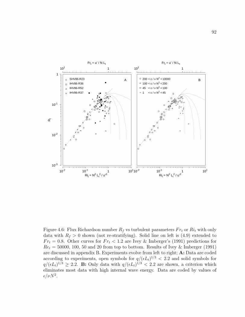
92
10-3
10-2
10-1
1
Rf
10-2 10-1 1 101
Rit = N2 Lt2 / u’2
ASHV86-R23
IHV86-R36
IHV86-R52
IHV86-R37
101 1
Frt = u’ / N Lt
10-2 10-1 1 101
Rit = N2 Lt2 / u’2
B200 < ε / ν N2 < 10000
100 < ε / ν N2 < 200
45 < ε / ν N2 < 100
1 < ε / ν N2 < 45
101 1
Frt = u’ / N Lt
Figure 4.6: Flux Richardson number Rf vs turbulent parameters Frt or Rit with onlydata with Rf > 0 shown (not re-stratifying). Solid line on left is (4.9) extended toFrt = 0.8. Other curves for Frt < 1.2 are Ivey & Imberger’s (1991) predictions forRet = 50000, 100, 50 and 20 from top to bottom. Results of Ivey & Imberger (1991)are discussed in appendix B. Experiments evolve from left to right; A: Data are codedaccording to experiments, open symbols for q/(ǫLt)
1/3 < 2.2 and solid symbols forq/(ǫLt)
1/3 ≥ 2.2. B: Only data with q/(ǫLt)1/3 < 2.2 are shown, a criterion which
eliminates most data with high internal wave energy. Data are coded by values ofǫ/νN2.

93
approximately by[
34± 1
4
]
Rit/3. There is no extra adjustment to make on
Γ ≈[
34± 1
4
]
Rit/3 for isotropy.
• The generalized form of Rit in terms of length scales combines both the inertial-
buoyancy balance and isotropy factors as Rit ≈ (Lh/LO)4/3 (Lh/LT )2 (using
ǫ ≈ u′3/Lh)
This is an important question for ocean turbulence which can be of low intensity
(ǫ/νN2 < 200) such that turbulence may become anisotropic (Gargett et al., 1984).
The effect of turbulent intensity on isotropy is difficult to ascertain using the
laboratory experiments. This might be because of the internal waves which stand out
at low turbulent intensity, and cloud the evaluation of turbulent kinetic energy and
its dissipation3. However, the effect of isotropy on the prediction of mixing efficiency
as Rit/3 can be examined.
Figure 4.7 shows the ratio of measured mixing efficiency Γ to the upper bound of
the expected mixing efficiency Rit/3—identical to the ratio of measured to expected
buoyancy flux—versus (A) the degree of isotropy w′/u′ and (B) versus turbulent
intensity ǫ/νN2. As expected, isotropy variations of 0.7 to 1 do not affect the predic-
tion of buoyancy flux from Rit. The buoyancy flux falls short of predictions only for
ǫ/νN2 < 45 where the Rit model fails. It is possible that internal wave contamination
is related to the observed cut-off value of ǫ/νN2 (see discussion in appendix A), or
that viscosity effects do in fact reduce buoyancy flux below ǫ/νN2 ≈ 45 as suggested
by Figure 4.7B.
In other words, the degree of isotropy affects Rit where departure from isotropy is
most noticeable for ǫ/νN2 < 100 (see Figure A.1). However, the resulting Rit seems to
predict the correct buoyancy flux. Figure 4.5 shows that, perhaps counter-intuitively,
anisotropy results in Rit < (Lt/LO)4/3. It is seen by comparing the isotropy-adjusted
Rit ≈ (Lt/LO)4/3(Lt/Lh)2/3 to the unadjusted (Rit)iso ≈ (Lt/LO)4/3 which over-
estimates the former.
3Figure A.1 described in appendix A shows that w′/u′ generally decreases for ǫ/νN2 less than afew hundred, except for a rise due to internal waves unrelated to turbulence.

94
0.5 1w’ / u’
10-2
10-1
1
101
Γ / (
Ri /
3)
= J
b / J
b m
odel
200 < ε / ν N2 < 10000
100 < ε / ν N2 < 200
45 < ε / ν N2 < 100
1 < ε / ν N2 < 45
1 101 102 103 104
ε / ν N2
SHV86-R23
IHV86-R36
IHV86-R52
IHV86-R37
Figure 4.7: Ratio of measured to predicted mixing efficiency versus isotropy w′/u′
and turbulent intensity ǫ/νN2. Vertical line in (B) is at ǫ/νN2 = 45. Experimentsevolve from high to low values of ǫ/νN2.

95
4.6 Relating the turbulent parameters to the large
scale
The applicability of the buoyancy flux model prediction (4.9) is limited. The turbulent
parameter Rit, while easily obtained in the lab, is not easily measured in the ocean.
The mixing efficiency parameterization in terms of Rit provides a useful framework,
as well as my earlier discussion on the significance of Frt, but they may require too
much knowledge about the state of the turbulence to be very useful.
In the previous chapter, it was hypothesized that Rit is related to the larger scale
gradient Richardson number Rig if turbulent velocities are produced from the mean
shear. The mixing efficiency could thus be inferred from measurements of Rig. This
model is tested now. If Rig is a useful substitute to Rit, then the parameterization
of Γ in terms of Rit allows large scale measurements to be used to infer the state of
the turbulence and its mixing efficiency.
The hypothesis is that
u′ = a LT∂U
∂z
or equivalently that
Rit =N2L2
T
a2L2T (∂U/∂z)2
=1
a2Rig
Figure 4.8 shows data from Rohr et al. (1988)4 and Stillinger (1981) conducted
in the same tank as the SHV and IHV experiments, but with the addition of a mean
shear flow.5
The value of Lt/LO is shown against the gradient Richardson number Rig =
N2/(∂U/∂z)2 where U is the mean velocity, now a function of depth. Turbulence
4Data from Rohr & Van Atta (1987) at three different values of Rig fit on the same line as theRohr et al. (1988) data.
5The data point from Tavoularis et al. (1981) should be disregarded. First, it is from an ex-periment in air (different Prandtl number). Second, they used Rig = (g/T )(∂T/∂z)/(∂U/∂z)2.Substituting their tabled values for Rig, ∂T/∂z and ∂U/∂z one gets T = 21. Unless these were verycold air experiments (not noted in the paper) they wrongly used temperature in degrees Celciusrather than Kelvin to calculate Rig. Third, the turbulence appears anisotropic. However, it shouldbe possible to check u′ = a LT ∂U/∂z from the original data.

96
Growing turbulence Decaying
Figure 4.8: Relation of turbulent parameter Lt/LO to gradient Richardson num-ber Rig for an grid turbulence experiment with a mean shear. Includes data fromStillinger (1981) and Tavoularis & Corrsin (1981). Figure reproduced from Rohr etal. (1988) (Their Figure 15). Note that (Rit)iso ≈ (Lt/LO)4/3 for isotropic turbulence.The slope of the line is 3/4 such that Rig ∝ Rit.

97
grows downstream for Rig < (Rig)cr, where (Rig)cr = 0.25. Recall that for isotropic
turbulence—as expected in the presence of a driving shear—the isotropic turbu-
lent Richardson number (Rit)iso is approximately equal to (Lt/LO)4/3, assuming
ǫ = u′3/LT (this scaling was shown to hold to better than a factor of two in Fig-
ure 4.5). In Figure 4.8 it is shown that for Rig < (Rig)cr in growing turbulence, the
gradient Richardson number is proportional to (Lt/LO)4/3, which is equal to (Rit)iso
The gradient Richardson number can therefore be related to the turbulent pa-
rameter Rit or Frt, which quantifies mixing efficiency in our model and in the grid
experiments discussed earlier. Thus, measurements of Rig, ξ and N are sufficient to
determine values of ǫ, Jb and Rf .
If models two and three were proved to be wrong, the fact that Rig is proportional
to (Lt/LO)4/3 and that Lt ≈ LT means that measurements of Rig and LT in the ocean
would yield indirect measurements of ǫ (but no indication of mixing efficiency).
The proportionality coefficient a will be discussed in the following sections.
4.6.1 Link Between the Rig–Rit Relation and Inertial-
Buoyancy Balance
The interpretation of Figure 4.8 implies a connection between the Rig–Rit relation and
the value of the turbulent Froude number at the inertial-buoyancy balance, (Frt)isoIB.
The Rig–(Rit)iso proportionality ends at (Rig)cr because gradient Richardson
numbers greater than (Rig)cr do not lead to instabilities and may not provide suffi-
cient shear to completely drive turbulence. Runs with Rig > (Rig)cr result in decaying
turbulence not unlike unsheared experiments, and the correlation between Rig and
Rit disappears. The value of Rit at Rig ≥ (Rig)cr is thus the inertial-buoyancy value:
the maximum value of Rit allowed in a turbulent flow, where the vertical kinetic
energy can just overcome buoyancy force.
The value of Rit at Rig ≥ 0.25 and the value Rit = a−2 (Rig)cr should be identical,
and represent the inertial-buoyancy balance values. They are identical within the
error bounds of Figure 4.8. Thus the proportion, a, of the velocity available to the

98
overturn from the shear, LT (∂U/∂z), that is converted to turbulent velocities, u′,
determines the inertial-buoyancy value of Rit at Rig = (Rig)cr. An empirical value
for a then follows from the inertial-buoyancy value of Rit, dicussed in the next section.
4.7 Inertial-Buoyancy Balance Value of Rit
The values of Rit and Lt/LO at the inertial-buoyancy balance are of interest for three
reasons: i) To determine the proportionality constant between Rig and Rit such that
the more commonly measured Rig can determine the state of the turbulence; ii) To
determine the maximum mixing efficiency predicted by the proposed model two as
≈ Rit/3; iii) To compare oceanic measurements of LT /LO to laboratory results in
relation to inertial-buoyancy balance values.
There is scatter in the Rig ∝ (Lt/LO)4/3 relation of Figure 4.8, ranging from
(Lt/LO)4/3 = 5.6 Rig to (Lt/LO)4/3 = 10.4 Rig (These values are taken by eye from
Figure 4.8 because the data were not tabulated). The corresponding ‘critical’ tur-
bulent Richardson numbers are (Rit)cr ≈ 1.4 to 2.6. For the decaying turbulence
at inertial-buoyancy balance (Rig > 0.25) in Figure 4.8, we find Lt/LO ≈ 1.45–1.7,
corresponding to Rit ≈ 1.65 to 2.03. The range of critical values of Rit is rather large
due to observational errors, but these seem to agree that it is greater than unity.
Maximum Mixing Efficiency in Grid Experiments
Returning to Figure 4.6, the maximum mixing efficiency expected at inertial-buoyancy
balance occurs at Rit = 0.7, much lower than anticipated from the experiments with
shear described above. There is thus an inconsistency to be resolved between these
data sets. The interpretation found in the original papers is described in appendix B.
With this inconsistency, one might wonder if the description in section 4.1.1 of
the evolution of the experiment is correct about the inertial-buoyancy balance decay
with constant ratio of LT /LO. Figure 4.6 suggests that mixing efficiency reaches a
peak before the decay stage, instead of thereafter remaining constant.
99
Figure 4.9 shows the downstream evolution of Thorpe scales LT and Ozmidov
scales LO in a grid-turbulence experiment without a mean shear. The experiment
evolves from right to left on the figure. Nearly a decade of inertial-buoyancy balance
decay was measured with constant LT /LO. There is again a lot of scatter, but I find
approximately LT /LO ≈ 1.5 during the decay, corresponding to (Rit)cr ≈ 1.7.
Thus the initial discussion in section 4.1.1 is consistent with other data, but not
with Figure 4.2, where all data in the late decay stage are contaminated by internal
waves. This helps to resolve the inconsistency. While it is possible that w′ρ′ correla-
tions are affected by internal waves, it is also possible that that my classification of
these data as internal waves and the mixing efficiency decrease are both symptoms of
turbulent kinetic energy extinction. If the internal waves were generated at the grid,
they would only become apparent when the initially much stronger turbulent energy
has decayed. Figure 4.10 shows the parameter space Lt/LO versus ǫ/νN2 covered
for the SHV and IHV data. The parameter space Lt/LO–ǫ/νN2 is highly correlated;
high intensity turbulence has low Rit and the reverse. It is difficult to separate the
effects of one parameter from the other on the turbulence, which could explain the
misinterpretation of decreasing mixing efficiency as related to Lt/LO, while it could
be due to low ǫ/νN2 values.
Data not identified as internal waves (q/(ǫLt)1/3 < 2.2) in Figure 4.10 have a wide
range of ǫ/νN2, but when the turbulence has evolved to an inertial-buoyancy balance
(Lt/LO ≈ 1.4) it can barely sustain a buoyancy flux, with ǫ/νN2 in the range 15 to
25.6 As discussed in section 4.5, it is possible that viscosity effects reduce buoyancy
flux below ǫ/νN2 ≈ 45 as suggested by Figure 4.7B. This is a lower turbulent intensity
than Gargett et al. (1984) reported for departure from isotropy. Perhaps anisotropy
occurs first during the decay, followed later by a reduction in mixing efficiency also
due to the effects of viscosity.
6The exact value of ǫ/νN2 needed to sustain a buoyancy flux is discussed in appendix A. Also,data with 10 < ǫ/νN2 < 100 fall in both categories of turbulence and internal waves, suggestingthat ǫ/νN2 is not the critical parameter to classify data as internal waves. As an additional test,the ratio q/(ǫLt)
1/3 was plotted against ǫ/νN2 and no value of ǫ/νN2 could consistently separateturbulence from internal waves for all experiments
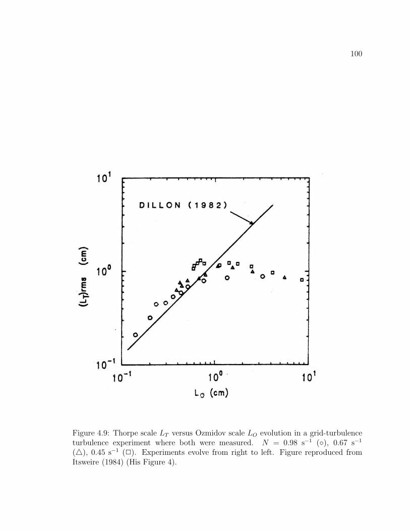
100
Figure 4.9: Thorpe scale LT versus Ozmidov scale LO evolution in a grid-turbulenceturbulence experiment where both were measured. N = 0.98 s−1 (◦), 0.67 s−1
(△), 0.45 s−1 (2). Experiments evolve from right to left. Figure reproduced fromItsweire (1984) (His Figure 4).
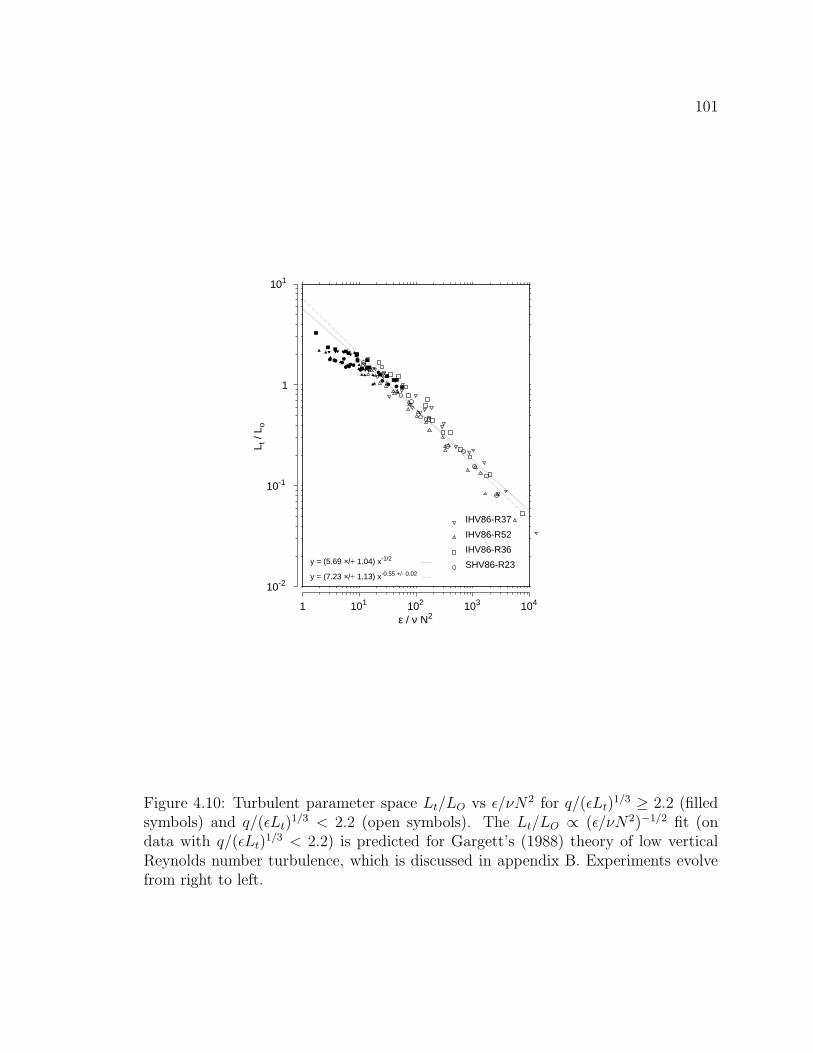
101
1 101 102 103 104
ε / ν N2
10-2
10-1
1
101
L t /
L o
SHV86-R23
IHV86-R36
IHV86-R52
IHV86-R37
y = (7.23 ×/÷ 1.13) x-0.55 +/- 0.02
y = (5.69 ×/÷ 1.04) x-1/2
Figure 4.10: Turbulent parameter space Lt/LO vs ǫ/νN2 for q/(ǫLt)1/3 ≥ 2.2 (filled
symbols) and q/(ǫLt)1/3 < 2.2 (open symbols). The Lt/LO ∝ (ǫ/νN2)−1/2 fit (on
data with q/(ǫLt)1/3 < 2.2) is predicted for Gargett’s (1988) theory of low vertical
Reynolds number turbulence, which is discussed in appendix B. Experiments evolvefrom right to left.

102
Thus, in summary, data sets from SHV and IHV cannot provide information about
the mixing efficiency during the inertial-buoyancy balanced decay because of the very
low turbulent intensity at that stage of the evolution (e.g. Figure 4.2). Other sketchy
data from Figure 4.8 from Rohr et al. (1988) and Stillinger (1981) and from Figure 4.9
reproduced from Itsweire (1984) indicate that the inertial buoyancy balance value of
Rit is in the range of 1.4 to 1.7. Taking a middle ground value of 1.55, one obtains a
maximum mixing efficiency of Γ ≈ Rit/3 ≈ 0.52 using the upper bound of (4.9). In
terms of turbulent Froude number, this becomes
(Frt)isoIB ≈ 0.8 (4.11)
The relation between velocity fluctuations and shear is thus given approximately
by
u′ ≈ 0.4 LT∂U
∂z(4.12)
where the factor of 0.4 comes from Rit = 1a2 Rig using critical values to determine a
from 1a2 ≈ 1.55/0.25 ≈ 6.2; This factor is only known approximately. Equivently, the
gradient and turbulent Richardson numbers are related approximately by
Rit ≈ 6.2 Rig (4.13)
4.8 Summary and Discussion
The main results of this chapter are that
• The Kolmogorov scaling for turbulent velocity fluctuations ǫ ≈ (u′3/Lt)(w′/u′),
where Lt is ρ′e/(∂ρ/∂z) and where Lt (u′/w′) is used to approximate the hori-
zontal turbulent length scale, was shown to hold (to much better than a factor
of two), at least for slight isotropy (w′/u′ varied from 0.7 to 1). Note that
turbulent velocities and length scales, buoyancy flux and TKE dissipation rates
are all time-averages at various locations behind the grid. It is not obvious how
these results can be extrapolated to individual overturns, or even to individual
profile measurements of a steadily forced mixing layer.

103
• ξ is well approximated by N2L2t /2 in the laboratory experiments.
• Mixing efficiency was well within a factor of two modelled by Rit/3, the upper
limit of the expected result for model two.
• Even though anisotropy reduces Rit, possibly as a result of viscosity at ǫ/νN2 <
200 (Gargett et al., 1984), the resulting Rit still models the mixing efficiency
well until about ǫ/νN2 < 45. This later value of mixing intensity is an upper
limit (The actual cutt-off value could be lower), as the lab data may contain
internal wave energy at this turbulent intensity. This implies that dividing the
measured APEF by a decay time would be a good estimate of buoyancy flux
for turbulent intensities as low as ǫ/νN2 ≈ 45
• Large and turbulent scales are related in the following way:
– Rit ≈ 1a2 Rig, from a model relating turbulent velocity fluctuations to
the mean shear and overturning scale as u′ ≈ a LT (∂U/∂z), where a is a
constant.
– The constant a was shown to be related to the inertial-buoyancy balance
of Rit, which in turn determines the maximum mixing efficiency of the
model.
The relation is such that (Frt)−2isoIB = (Rit)cr ≈ 1
a2 (Rig)cr, where (Rit)cr
is the inertial-buoyancy value and (Rig)cr = 0.25
– The value of (Rit)cr is uncertain with current data, but seems to be ap-
proximately 1.55 (at best within a factor of two).
The corresponding turbulent Froude number at isotropic inertial-buoyancy
balance is (Frt)isoIB ≈ 0.8 This corresponds to a ≈ 0.4 using (Rig)cr =
0.25.
This corresponds to Rit ≈ 6.2 Rig
The above results tend to substantiate the major assumptions and predictions of
the second model of chapter 3 for isotropic growing turbulence, for which buoyancy

104
flux is given by ξ divided by a timescale set by turbulent overturning. This is true
at least for averaged data, where redistribution of kinetic and potential energy can
also be neglected. The extrapolation to single sampling profiles of a mixing layer is
unclear.
Another implication is that model one, which assumes a constant mixing efficiency,
would over-estimate buoyancy flux by 2 orders of magnitude in the early stages of
growth in these laboratory experiments. Model one would have to be set aside if
mixing efficiency (and Frt) is found to vary likewise in the ocean (not always at
inertial-buoyancy balance), although it is likely to hold for breaking internal waves in
the ocean interior.
The determination of the inertial-buoyancy balance value of Rit is problematic.
The lab experiments are not well designed for this purpose. The initial overturn
size, mostly determined from the grid mesh size, is too small relative to the Ozmidov
scale LO = (ǫ/N3)1/2, which is fairly close to the final overturn size at the end
of growth. Turbulent intensity falls off before turbulence fully evolves to inertial-
buoyancy balance. A proper parameter range would show a knee in Figure 4.10: the
increase of Lt/LO would stop, while values of ǫ/νN2 would continue to decrease. The
flat Lt/LO range would correspond to the inertial-buoyancy balanced decay.
Future experiments should focus on the inertial-buoyancy balance to better quan-
tify (Rit)cr. The parameter is important because it determines the maximum mixing
efficiency possible. Perhaps more importantly, (Rit)cr also determines the proportion-
ality coefficient between the gradient Richardson number and the turbulent Richard-
son number.
However, these considerations assume that these results are relevant to the ocean.
Questions must be answered before this can be assumed. Does the ocean mix at a
wide range of turbulent Richardson numbers leading to a range in mixing efficiencies?
Or does the ocean mixing layers quickly evolve to steady-state isotropic turbulence at
inertial-buoyancy balance? If so, can my predicted inertial-buoyancy balance mixing

105
efficiency (for isotropic turbulence) of 0.5 be reconciled with Oakey’s (1985) result7
of 0.40. These questions is will addressed in the next 2 chapters.
7Oakey(1985) obtains Γ = 0.265 assuming a factor of 2 (partial) rather than 3 (full) for isotropy.

Chapter 5
Comparison of the Mixing Models
in the Ocean
In this chapter, oceanic and fresh water turbulence data reported by Dillon (1982)
and used again by Dillon (1984) and Dillon et al. (1987) are used with the following
purposes in mind:
• To test the 3 models put forward in chapter 3 with oceanic data.
• To compare Dillon’s models to each other. Dillon et al. (1987) put forward an
empirical relation between buoyancy flux and ξ N , but never compared it to
earlier relations between the buoyancy flux and LT and between the dissipation
of turbulent kinetic energy and LT (Dillon, 1982).
• To determine the value of the turbulent Froude number Frt at isotropic inertial-
buoyancy-balance . This value is important because it determines the maximum
mixing efficiency and the constant relating Rit to Rig.
• To determine the range of Frt and Γ values for oceanic turbulence to see if model
two and three are really any different from model one in oceanic conditions.
The Dillon data set is divided in cases called A, B and C in this chapter. The reader
is referred to appendix C for a description of the cases, and of Dillon’s results. The
106

107
data were obtained at Ocean Station P during the MILE experiment (Series A and B)
and at Green Peter Reservoir (Series C). All of Dillon’s data are mostly temperature-
stratified such that temperature Thorpe fluctuations T ′ will be used instead of using
density fluctuations ρ′ (see appendix C). The turbulent Froude number Frt was not
measured by Dillon, but layer-averages for ǫ, N , and LT will make it possible to extract
Frt and to calculate the buoyancy flux predicted by the models. Measurement of the
dissipation of temperature variance χθ are also available for the layers. These can be
related easily to the potential energy dissipation. The approximation that this term
equals Jb is made throughout this chapter. Buoyancy flux predictions can then be
compared to overturn-scale observations.
5.1 Calculation of N2
The APEF must be evaluated to compare model predictions for Jb from chapter 3 to
observations. Dillon first defined the APEF in his 1984 paper; it is not tabulated in
his 1982 paper along with other layer-averaged quantities. An approximation must
therefore be made using the stratification against which work is done by overturning.
However, this stratification definition may differ from the large scale stratification
used, for example, in parameterizing mixing rates in terms of Kρ. Dillon’s layer
averages are examined here to determine if his tabled values of N2 are large scale
parameterization or representative of the overturns.
In Chapter 2, it was shown that ξ was well approximated by N2L2T /2 when N2 =
(g/ρ) ∂ρ/∂z is calculated by a least-squares fit on the re-ordered density profile of
an overturn. However, a larger-scale parameterization with N obtained over a span
containing non-overturning portions led to overestimating ξ by a factor of 2 to 2.4
for the layer, since the stratification is lower within overturns1. Dillon calculated N2
over 50 cm segments of the re-ordered profiles, and averaged together the segments
associated with overturns, sometimes enclosing 25–50 cm outside of the overturns.
1Crawford (1986) does a similar analysis and finds that ξ is overestimated by a factor of 2.8 whenbulk stratification is used.

108
When the span of an individual overturn was not obvious, parameters were averaged
over a depth span of similar statistical distributions. Thus the averaging spans of
data tabled by Dillon (1982) should be somewhere in between overturn spans and a
large-scale parameterization.
In chapter 2, it was shown that if LT ≈ T ′21/2/(∂To/∂z) then ∂To/∂z was repre-
sentative of overturns instead of larger scales (In chapter 2, density fluctuations were
used instead of temperature). Figure 5.12 tests this, using values of ∂To/∂z, LT and
T ′. There is little scatter for the two oceanic cases A and B, with an average on the
mean of ∂To/∂z = 1.85 T ′21/2/LT . (from T ′21/2
/LT = 0.54 ∂To/∂z, since regressions
were performed minimizing variance in the ordinate) In Chapter 2 statistics on a mix-
ing patch in the St. Lawrence estuary yielded ∂To/∂z = 0.93 T ′21/2/LT when ∂To/∂z
was evaluated over distinct overturns, and ∂To/∂z = 2.14 T ′21/2/LT when ∂To/∂z was
evaluated over spans enclosing many overturns. Thus the data in Series A and B seem
to have been evaluated over spans which include sharper gradients than those found
within the overturns. Series C, the fresh water case, has many points with ∂To/∂z
greatly exceeding T ′21/2/LT . This can lead to great errors in the models put forward
in this chapter, as well as in the estimated measured buoyancy flux αgχθ/2(∂T/∂z).
Because N2 is representative of larger scales than overturns, the APEF approxima-
tion N2L2T /2 is expected to over-estimate by a factor of 2 (from the above comparison
of T ′21/2/LT = 0.54 ∂To/∂z). Verifying the buoyancy flux models from chapter 3 using
this approximation would result in extra scatter. The only APEF approximation using
larger scale averages that was shown to work in chapter 2 is ξ ≈ (1/2)(g/ρ)ρ′21/2LT .
We will show in the next section that this relation does in fact lead to less scatter
compared to buoyancy flux.
2The regressions shown in Figure 5.1, as well as in all log–log figures in this chapter, are performedin logarithmic space. The confidence interval on the mean is expressed as 10a±ci = 10a ×/÷ 10ci.

109
Series C
10-3
10-2
10-1
1
101
T’ /
LT
10-3 10-2 10-1 1 101
∂ T/∂ z
200 < ε / ν N2
100 < ε / ν N2 < 200
45 < ε / ν N2 < 100
ε / ν N2 < 45
y = (0.28 ×/÷ 1.41) x0.78 +/- 0.16
y = (0.39 ×/÷ 1.30) x
Series A
10-3
10-2
10-1
1
101
T’ /
LT
200 < ε / ν N2
100 < ε / ν N2 < 200
45 < ε / ν N2 < 100
ε / ν N2 < 45
y = (0.19 ×/÷ 1.33) x0.74 +/- 0.07
y = (0.51 ×/÷ 1.20) x
10-3 10-2 10-1 1 101
∂ T/∂ z
Series A and B
200 < ε / ν N2
100 < ε / ν N2 < 200
45 < ε / ν N2 < 100
ε / ν N2 < 45
y = (0.27 ×/÷ 1.25) x0.83 +/- 0.06
y = (0.47 ×/÷ 1.13) x
Series B
200 < ε / ν N2
100 < ε / ν N2 < 200
45 < ε / ν N2 < 100
ε / ν N2 < 45
y = (0.39 ×/÷ 1.42) x0.96 +/- 0.13
y = (0.43 ×/÷ 1.18) x
Figure 5.1: Comparison of estimated temperature gradient within overturns T ′21/2/LT
to measured gradient ∂To/∂z for two oceanic cases (Series A and B) and a fresh waterreservoir (Series C). The gradient ∂T/∂z is evaluated on the re-ordered profile over
overturn-containing spans; T ′21/2/LT is an estimate of the local gradient within the
overturns and is found to be lower than ∂To/∂z. Data are classified by turbulentintensity ǫ/νN2. Open symbols are well resolved; filled symbols are marginally re-solved. Regression are on points with ǫ/νN2 > 200. Data are from tables in Dillon(1982).

110
5.2 Dillon’s Relations
In this section, the models inferred from Dillon’s relations LT –LO and LT –LB (ex-
plained in appendix B) are examined more closely and discussed. Dillon compared
the LT –LO and LT –LB relations, but did not compare his later Jb = 4.8 ξ N model
to the first two. His first two models are related to the APEF and its commonly used
approximation N2L2T /2.
The results of chapter 2 will be confirmed, showing that the density gradient within
overturns is well approximated by bulk properties as ρ′21/2
/LT , such that the APEF
approximation N2L2T /2 works well by substituting that gradient into the expression
for N2. Also confirmed will be that N2L2T /2 over-estimates ξ by a factor of two if a
bulk N2 is used.
Of Dillon’s relations, the one that best matches his data will be determined, such
that it can be related to and compared to the models from chapter 3.
5.2.1 Relationship Between ǫ and LT
The relation LT /LO = 1.17 was found to hold for oceanic series B (see appendix B,
Figure C.1) Substituting the definition of LO = (ǫ/N3)1/2 leads to
ǫ ≈ 0.7L2T N3 (5.1)
using N2 calculated over a larger scale than that of the overturns.
This is identical to the first model from chapter 3 (apart from the coefficient): the
traditional view relating overturns to mixing.
5.2.2 Buoyancy Flux Relation to Thorpe Scale
Dillon’s relation LT /LB = 1.23, where LB = (Jb/N3)1/2 leads to
Jb ≈ 0.65L2T N3 (5.2)
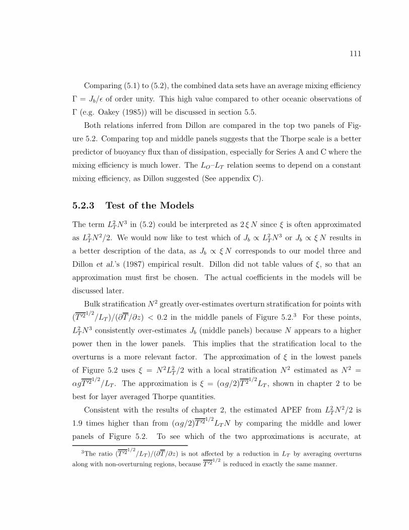
111
Comparing (5.1) to (5.2), the combined data sets have an average mixing efficiency
Γ = Jb/ǫ of order unity. This high value compared to other oceanic observations of
Γ (e.g. Oakey (1985)) will be discussed in section 5.5.
Both relations inferred from Dillon are compared in the top two panels of Fig-
ure 5.2. Comparing top and middle panels suggests that the Thorpe scale is a better
predictor of buoyancy flux than of dissipation, especially for Series A and C where the
mixing efficiency is much lower. The LO–LT relation seems to depend on a constant
mixing efficiency, as Dillon suggested (See appendix C).
5.2.3 Test of the Models
The term L2T N3 in (5.2) could be interpreted as 2 ξ N since ξ is often approximated
as L2T N2/2. We would now like to test which of Jb ∝ L2
T N3 or Jb ∝ ξ N results in
a better description of the data, as Jb ∝ ξ N corresponds to our model three and
Dillon et al.’s (1987) empirical result. Dillon did not table values of ξ, so that an
approximation must first be chosen. The actual coefficients in the models will be
discussed later.
Bulk stratification N2 greatly over-estimates overturn stratification for points with
(T ′21/2/LT )/(∂T/∂z) < 0.2 in the middle panels of Figure 5.2.3 For these points,
L2T N3 consistently over-estimates Jb (middle panels) because N appears to a higher
power then in the lower panels. This implies that the stratification local to the
overturns is a more relevant factor. The approximation of ξ in the lowest panels
of Figure 5.2 uses ξ = N2L2T /2 with a local stratification N2 estimated as N2 =
αgT ′21/2/LT . The approximation is ξ = (αg/2)T 21/2
LT , shown in chapter 2 to be
best for layer averaged Thorpe quantities.
Consistent with the results of chapter 2, the estimated APEF from L2T N2/2 is
1.9 times higher than from (αg/2)T ′21/2LT N by comparing the middle and lower
panels of Figure 5.2. To see which of the two approximations is accurate, at
3The ratio (T ′21/2
/LT )/(∂T/∂z) is not affected by a reduction in LT by averaging overturns
along with non-overturning regions, because T ′21/2
is reduced in exactly the same manner.
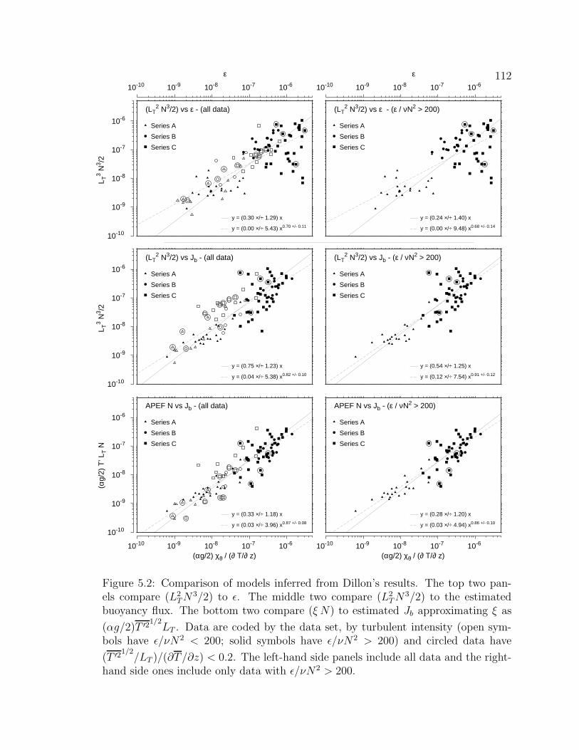
112
APEF N vs Jb - (all data)
10-10
10-9
10-8
10-7
10-6
(αg/
2) T
’ LT N
10-10 10-9 10-8 10-7 10-6
(αg/2) χθ / (∂ T/∂ z)
Series A
Series B
Series C
y = (0.03 ×/÷ 3.96) x0.87 +/- 0.08
y = (0.33 ×/÷ 1.18) x
APEF N vs Jb - (ε / νN2 > 200)
10-10 10-9 10-8 10-7 10-6
(αg/2) χθ / (∂ T/∂ z)
Series A
Series B
Series C
y = (0.03 ×/÷ 4.94) x0.86 +/- 0.10
y = (0.28 ×/÷ 1.20) x
(LT2 N3/2) vs Jb - (all data)
10-10
10-9
10-8
10-7
10-6
L T3 N
3 /2
Series A
Series B
Series C
y = (0.04 ×/÷ 5.38) x0.82 +/- 0.10
y = (0.75 ×/÷ 1.23) x
(LT2 N3/2) vs Jb - (ε / νN2 > 200)
Series A
Series B
Series C
y = (0.12 ×/÷ 7.54) x0.91 +/- 0.12
y = (0.54 ×/÷ 1.25) x
(LT2 N3/2) vs ε - (all data)
10-10
10-9
10-8
10-7
10-6
L T3 N
3 /2
10-10 10-9 10-8 10-7 10-6
ε
Series A
Series B
Series C
y = (0.00 ×/÷ 5.43) x0.70 +/- 0.11
y = (0.30 ×/÷ 1.29) x
(LT2 N3/2) vs ε - (ε / νN2 > 200)
10-10 10-9 10-8 10-7 10-6
ε
Series A
Series B
Series C
y = (0.00 ×/÷ 9.48) x0.68 +/- 0.14
y = (0.24 ×/÷ 1.40) x
Figure 5.2: Comparison of models inferred from Dillon’s results. The top two pan-els compare (L2
T N3/2) to ǫ. The middle two compare (L2T N3/2) to the estimated
buoyancy flux. The bottom two compare (ξ N) to estimated Jb approximating ξ as
(αg/2)T ′21/2LT . Data are coded by the data set, by turbulent intensity (open sym-
bols have ǫ/νN2 < 200; solid symbols have ǫ/νN2 > 200) and circled data have
(T ′21/2/LT )/(∂T/∂z) < 0.2. The left-hand side panels include all data and the right-
hand side ones include only data with ǫ/νN2 > 200.

113
least in an average sense, we compare it to Dillon et al.’s (1987) calculation of a
mean (αgχθ/2∂T/∂z)/(ξ N) ratio, using the definition form of the APEF. Here I
am assuming that buoyancy flux equals the dissipation of potential energy Jb =
(αg/2)χθ/(∂T/∂z) (e.g. Equation (3.10) assuming that the time-derivative is zero);
Dillon et al. (1987) did not require this assumption, comparing ξN to the dissipa-
tion of potential energy without assumptions about Jb. Dillon et al. (1987) found
Jb/(ξ N) = 4.8 (replacing the dissipation of potential energy by simply Jb in the
notation, whereas a similar calculation in linear space yields Jb/ (αg/2)T ′21/2LT N
= 4.38. This indicates that (αg/2)T ′21/2LT is a good approximation of ξ, and that
N2L2T /2 is an over-estimate by a factor of two, as predicted from Figure 5.1.
Comparing the middle and lower panels of Figure 5.2 tests which of Jb ∝ L2T N3 or
Jb ∝ ξ N results in the better fit. Note that even in the ξ N panel, there is a slight bias
toward over-estimating Jb for data with ǫ/νN2 < 200, although this is mostly true in
Series C, the fresh water case. Those data have been removed from the least squares
fit regression in the right-hand panels. Since data with (T ′21/2/Lt)/(∂T/∂z) < 0.2
yield a better fit in the lower panels of Figure 5.2 than in the middle panels, and that
the fit for all data appears (judged by eye only, as the statistics only yield confidence
errors on the mean, not information on the variance explained by the regression) to be
generally better in the lower panels, we conclude that using a better approximation
of ξ appears to result in a better fit to Jb using a decay time of N−1 for the APEF.
Dillon et al.’s (1987) last relation for buoyancy flux from the APEF, as Jb = 4.8 ξ N
is then his best fitting for buoyancy flux. The LT –LO relation is incidental. It requires
that the mixing efficiency is constant, which is not a general result (see Appendix C
and Figure 5.4 for details).

114
5.3 Comparison of Models Two and Three to Dil-
lon’s Data
Dillon’s best-fitting relation to his data is Jb = 4.8 ξ N (assuming that the buoy-
ancy flux equals the potential energy dissipation). Except for the coefficient, this
is my third model, describing turbulence at inertial-buoyancy where the horizontal
turbulent length scale has evolved to the Ozmidov (inertial-buoyancy) length scale
LO.
Let us now compare Dillon’s data to both my second and third models. The aim
is to see if one is preferable to the other for Dillon’s data.
As just discussed, the third model is written as
Jb =[
3
4±
1
4
]
ξ N =[
3
4±
1
4
]
αg
2T ′21/2
LT N (5.3)
The discrepancy between the model’s coefficient and that of Dillon et al.’s (1987)
result of Jb = 4.8 ξ N will be discussed later.
5.3.1 Model Two Re-derived
To compare data with model two, it must be written in a form which minimizes
approximations. Recall that the second model describes growing isotropic turbulence.
It is written as
Jb =[
3
4±
1
4
]
2
3ξ N Frt (5.4)
Unfortunately, the turbulent Froude number is not (usually) a measured quantity
in the ocean, nor was it in Dillon’s data. Since ǫ was measured and ξ can be ap-
proximated, a form such as (3.23) could be used to infer Frt and yield (3.24) as the
second model’s buoyancy flux. However, the derivation of (3.23) assumed that ξ was
well approximated by N2L2T /2 which has be shown not to be true for this data set.
A buoyancy flux prediction for the second model is now derived using approxi-
mations that best employ the data available. Using the scaling ǫ ≈ u3/LT which

115
has been shown to hold quite well for grid-turbulence (this model assumes isotropy,
LT = Lh), the tubulent Froude number can be written
Frt =u′
NLT
=ǫ1/3
NL2/3T
(5.5)
such that the APEF approximation N2L2T /2 usually used is avoided. Combining (5.4)
and (5.5), and using the better APEF approximation ξ = (αg/2)T ′21/2LT , we obtain
an expression for the buoyancy flux of the second model as4
Jb =[
3
4±
1
4
]
αg
3T ′21/2
L1/3T ǫ1/3 (5.6)
5.3.2 Comparisons of the Models
The grid-turbulence experiments agreed with the upper bound of the second model
in chapter 4. In that case, the turbulence was obviously growing because it is created
at small scales by a grid. In the ocean, the state of the turbulence is unknown and
either the isotropic growing turbulence model, or the steady-state inertial-buoyancy
balance model could hold.
The upper bound of the buoyancy flux predictions (5.3) and (5.6) are compared
to the measured potential energy dissipation in Figure 5.3. Differences are subtle,
especially if only high turbulent intensity data are considered (see right hand panels).
It would be difficult to convince anyone to use one model rather than the other with
the slight gains that would be afforded. It is possible that the dynamics of the mixing
layers is sometimes appropriate to the second model (growing turbulence) and some
other times appropriate to the third (steady-state). Data from case C appear to have
less scatter in the the second model (Jb ∝ ξ N Frt). The next section investigates
model differences further.
4The N cancels out by combining (5.4) and (5.5) to obtain (5.6), but in fact it never entersthe equation when it is considered using the decay time. Starting with Jb =
[
3
4± 1
4
]
ξ t−1o , where
to = (3u′2/2)/ǫ, the same substitution used in (5.5) gives t−1o = (2/3)L
2/3
T ǫ−1/3. Buoyancy fluxis then given by (5.6) without ever using N . This means that (5.6) is not sensitive to large scale
parameterisation of N2 = αg(∂T/∂z) 6= αg(T ′21/2
/LT ).

116
(2/3) APEF N Frt vs Jb - (all data)
10-10
10-9
10-8
10-7
10-6
(αg/
3) T
’ LT
1/3 ε
1/3
10-10 10-9 10-8 10-7 10-6
(αg/2) χθ / (∂ T/∂ z)
Series A
Series B
Series C
y = (0.05 ×/÷ 3.46) x0.90 +/- 0.07
y = (0.26 ×/÷ 1.16) x
(2/3) APEF N Frt vs Jb - (ε / νN2 > 200)
10-10 10-9 10-8 10-7 10-6
(αg/2) χθ / (∂ T/∂ z)
Series A
Series B
Series C
y = (0.03 ×/÷ 4.05) x0.87 +/- 0.09
y = (0.24 ×/÷ 1.18) x
APEF N vs Jb - (all data)
10-10
10-9
10-8
10-7
10-6
(αg/
2) T
’ LT N
Series A
Series B
Series C
y = (0.03 ×/÷ 3.96) x0.87 +/- 0.08
y = (0.33 ×/÷ 1.18) x
APEF N vs Jb - (ε / νN2 > 200)
Series A
Series B
Series C
y = (0.03 ×/÷ 4.94) x0.86 +/- 0.10
y = (0.28 ×/÷ 1.20) x
Figure 5.3: Comparison of two derivations of the buoyancy flux models from Chap-
ter 3. The top two panels compare (ξ N) to Jb approximating ξ as (αg/2)T ′21/2LT
(and Jb is approximated by the dissipation of potential energy in all panels). The bot-tom panels compare ((2/3)ξNFrt) to Jb, where (2/3)ξNFrt is best approximated by
(αg/3)T ′21/2L
1/3T ǫ1/3 for Dillon’s tabled data. Data are coded by the data set, by tur-
bulent intensity (open symbols have ǫ/νN2 < 200; solid symbols have ǫ/νN2 > 200)
and circled data have (T ′21/2/LT )/(∂T/∂z) < 0.2. The left-hand side panels include
all data and the right-hand side ones include only data with ǫ/νN2 > 200.

117
5.4 Comparison of Mixing Efficiencies
The main difference in the predictions between the isotropic growing turbulence model
(5.4) and the anisotropic fully developed turbulence model (5.3) is that the first is
dependent on Frt and the other is not; this translates to one being dependent on ǫ
in (5.6) and the other not in (5.3). The models predict similar buoyancy fluxes only
where physics converges: at inertial-buoyancy balance and at isotropy. Both of these
parameters determine the ratio L2T /(L
4/3O L
2/3h ) which quantifies the mixing efficiency
for both models. Comparison of the mixing efficiencies predicted by the two models
with the measured mixing efficiency should highlight any differences between models.5
Model 2; Isotropic Case
For the isotropic model, the predicted mixing efficiency is written as
Γ =[
3
4±
1
4
]
αg
3T ′21/2
L1/3T ǫ−2/3 (5.7)
using Γ = Jb/ǫ and (5.6).
Model 3; Steady-State Case
For the steady-state inertial-buoyancy balance model, the predicted mixing efficiency
is
Γ =[
3
4±
1
4
]
αg
2T ′21/2
LT N ǫ−1 (5.8)
using (5.3).
5If the LO = (ǫ/N3)1/2 parameterisation were done using N local to overturns, two relationsfor mixing efficiency could easily be compared: Γ = (LT /LO)4/3/3 for the isotropic case and Γ =(LT /LO)2/2 for the non-isotropic case. Unfortunately, a correction must be made because ∂T/∂z 6=
T ′21/2
/LT . The analysis becomes complicated and, as it turns out, is not conclusive. It is thereforenot included here.

118
5.4.1 Predicted Mixing Efficiency Comparison
In Figure 5.4, the model predictions are compared to the measured mixing efficiency.
The regressions have large confidence intervals on the slopes, and so were also per-
formed by least squares on the abscissae as well as on the usual ordinates. The
geometric mean of the two slopes yields the ‘geometric mean of the function regres-
sion of the ordinate on the abscissa’, also called the GM regression (Ricker, 1973). It
represents a better estimate of the slope if errors exist in both the abscise and the
ordinate.
The predicted and measured mixing efficiency have a GM regression power law
very close to unity for the combined series A and B using the third model (Figure 5.4D,
highlighted). Using this criterion, the steady-state model three is a better predictor
for those data. Forcing a power law of unity, the best fit is
Γmodel 3 = (0.28×/÷1.21) Γmeasured (5.9)
However, series C is not well fitted by either model. The model coming closest to
a one-to-one power law is the isotropic model (Figure 5.4A, highlighted). The GM
regression is a power law of 1.2. Forcing a power law of unity, the best fit for series C
is
Γmodel 2 = (0.31×/÷1.27) Γmeasured (5.10)
In conclusion, Series A and B are quite different from Series C. Oceanic series
A and B are found to marginally match predictions for the buoyancy flux model
derived from the APEF dissipated in a time scale N−1, at least within a multiplicative
constant. Fresh water series C data have more scatter, and could be marginally
associated with the isotropic turbulence model of growing turbulence.
In both cases, the predicted mixing efficiency is 3 times lower than the measured
mixing efficiency. This is discussed next.

119
C- Model 3
10-3
10-2
10-1
1
101
(α g
/2)
T’ L
T N
/ ε
10-2 10-1 1 101
Γ
Series C
y = (0.40 ×/÷ 2.30) x1.21 +/- 0.44
x = (0.61 ×/÷ 1.63) y0.41 +/- 0.15
D- Model 3
10-2 10-1 1 101
Γ
Series A
Series B
y = (0.28 ×/÷ 1.20) x0.78 +/- 0.19
x = (2.88 ×/÷ 1.38) y0.83 +/- 0.20
y = (0.28 ×/÷ 1.21) x
A- Model 2
10-3
10-2
10-1
1
101
(α g
/3)
T’ L
T1/
3 ε-2
/3Series C
y = (0.25 ×/÷ 1.80) x0.87 +/- 0.31
x = (0.94 ×/÷ 1.87) y0.58 +/- 0.21
y = (0.31 ×/÷ 1.27) x
B- Model 2
Series A
Series B
y = (0.18 ×/÷ 1.15) x0.54 +/- 0.14
x = (6.68 ×/÷ 1.72) y1.13 +/- 0.29
Figure 5.4: Mixing Efficiency compared to Models. A- Second model mixing efficiencyprediction versus measure mixing efficiency for series C. GM regression has Γmodel ∝Γ1.2; B- Second model for series A and B. GM regression has Γmodel ∝ Γ0.7; C- Thirdmodel for series C. GM regression has Γmodel ∝ Γ1.7; D- Third model for series A andB. GM regression has Γmodel ∝ Γ0.97; All regression are on data with ǫ/νN2 > 200.Thick lines are x regressed on y; thin lines are y regressed on x, solid lines have forcedslope and dashed lines have best fitting slopes. Highlighted panels A and D indicatebest fitting model.

120
5.5 Possible Bias in the Dillon Data Set
If both the buoyancy flux and mixing efficiency of Dillon’s data are much higher than
predicted by either the second or third model, then either the models are wrong or
the data set is biased. While the mean mixing efficiency of the data set is close to
unity, many individual values are above 1. In fact, 24 of the 56 data points of Series
A and B have Γ > 1.
Oakey (1985) obtains Γ from simultaneous measurements of both χθ and ǫ in
275 10–15 m blocks. He finds values ranging from 0.01 to 1, with a mean of 0.265
(assuming a log-normal distribution) and one standard deviation confidence interval
as 0.066 < Γ < 0.436.6 Thus, Dillon’s mixing efficiency seems high in comparison.
Possible bias could come from errors in ∂T/∂z, ǫ or χθ. These will be considered
in turn, althought it must be emphasized that there is no proof that any of Dillon’s
data are biased; they simply do not match models shown here, and have unusually
high mixing efficiencies.
5.5.1 Possible Bias in ∂T/∂z
The stratification N2 = αg(∂T/∂z), averaged over a layer containing many overturns,
has been shown to over-estimate the re-ordered density gradient within overturns,
such that T ′21/2/LT > ∂T/∂z. An APEF approximation insensitive to this error was
used, but a multiplication by an uncorrected N remains in the third model expression
for mixing efficiency (5.8).
A rationale for the better APEF approximation used is as follows: if overturning
statistics are averaged within a bin, but the APEF comes from one overturn within
that bin, then using T ′21/2/LT to approximate the overturn’s density gradient makes
6Oakey uses a lower isotropy coefficient, namely Jb = (αg/3)χθ/(∂T/∂z) such that his valuesshould be multiplied by 1.5 to be compared with Dillon’s. Alternatively, Dillon’s values could beadjusted to Oakey’s. We choose here to assume full isotropy for consistency with earlier derivationswhich assumed it also.

121
more sense than using ∂T/∂z. The same argument could be used for the the dissi-
pation of potential energy. If all the temperature fluctuation variance is dissipated
within that overturn as well, then the dissipation of potential energy ∝ (∂T/∂z)−1
should be better approximated substituting T ′21/2/LT for ∂T/∂z.
Unfortunately, if T ′21/2/LT is used in place of ∂T/∂z in the calculation of the
dissipation of potential energy and the buoyancy flux expression of the third model
(5.3), then the discrepancy increases further between (5.3) and the dissipation of
potential energy. This correction could not bring Dillon’s data in line with models
two and three.
5.5.2 Possible Bias in ǫ
Let us consider the possibility that dissipation of turbulent kinetic energy is under-
estimated. The buoyancy flux prediction from the third model (5.3) is not a function
of ǫ. Therefore, ǫ adjustments have no effect on fits with observations, either in terms
of buoyancy flux or mixing efficiency.
On the other hand, the buoyancy flux of the second model (5.6) is proportional
to ǫ1/3. The model’s buoyancy flux must be increased by a factor of three to fit the
observations. This requires an increase of ǫ by a factor 27, and would make mixing
efficiencies 27 times lower. This is such a large factor that it is unlikely that Dillon’s
observed mixing efficiency can be brought into line with the models by presuming
that a bias in ǫ exists.
5.5.3 Possible Bias in χθ
Changes in χθ have no bearing on predictions of buoyancy flux or mixing efficiency for
either model. Therefore, all observations of buoyancy flux and mixing efficiency would
be consistent with the models, and with Oakey’s observations of mixing efficiency, by
reducing χθ by a factor of 3.
Dillon (1982) approximates his error level in χθ as 30%. This is of course not com-
patible with my suggestion that χθ is over-estimated by a factor of 3. Nevertheless,

122
for Dillon to be correct about both χθ and ǫ implies that he has measured a mean
mixing efficiency of order unity and measured maximum values of ≈ 4. These num-
bers are unusually high (e.g. Oakey (1985) obtains Γ from 0.01 to 1, with a mean of
0.265). Note that Marmorino (1991) plotted observations of LT versus (κT Cx/N)1/2,
equivalent to showing 12L2
T N3 versus N2κT Cx, and obtained values of N2κT Cx from
half to a tenth of the values of Dillon. These arguments taken together suggest that
Dillon’s measurements of χθ are over-estimated by a factor of 3. If this were the case,
series A and B would then be consistent with my third model, and series C would be
marginally consistent with my second model.
5.6 Summary
In this chapter, the buoyancy flux models of chapter 3 were tested on Dillon’s data
sets consisting of two oceanic cases (Series A and B) and one fresh water reservoir
(Series C). The results are summarized as follows:
• Dillon’s (1982) verification of the Ozmidov scale LO relation to the Thorpe scale
LT holds only for series B. In that case the turbulent Froude number Frt, and
therefore the mixing efficiency, does not vary much. This is equivalent to model
one discussed in chapter 3, relating the rate of dissipation of turbulent kinetic
energy to ξN . It is not a general result because it fails in series A and C, with
surface mixed layer data. This is not a new result as Dillon (1982) noted this,
but it is included here to contrast model one with models two and three.
• Dillon’s layer averages were shown to include non-overturning parts of the water
column. The stratification listed by Dillon over-estimates stratification local to
overturns. The APEF approximation N2L2T /2 is an over-estimate by a factor
of 2 to 3 for this data.
– As a corollary, the ratio of LT /LO is ambiguous even when used to quantify

123
the inertial-buoyancy balance value; this usage was discussed for grid-
turbulence. The reason is that the value of LO = (ǫ/N3)1/2 obtained
depends on how N2 is evaluated. In this case, N2 is a layer-average (see
section 5.1). For the lab experiments, it measured the stratification that
overturns worked against. This makes comparisons difficult.
• Dillon et al.’s (1987) empirical relation Jb = 4.8ξ N better fits his data than
earlier models ǫ ∝ L2T N3 and Jb ∝ L2
T N3. In the second case, it is because
N2L2T /2 only approximates ξ. Dillon et al.’s (1987) empirical relation is consis-
tent with the third model, except for a much higher coefficient used by Dillon
et al. (1987).
• Dillon’s series A and B are consistent with the third model, which assumes
inertial-buoyancy balance. The Ozmidov scale LO is the horizontal turbulent
length scale Lh, generally greater than the Thorpe scale LT representing the
vertical turbulent length scale. The buoyancy flux is related to the decay of the
APEF over a time scale N−1.
• Dillon’s fresh water series C is somewhat consistent with the second model.
It describes growing isotropic turbulence. The buoyancy flux is related to the
decay of the APEF over a time scale (3/2)L−2/3T ǫ1/3.
• While both models are consistent with different parts of the data, the predicted
buoyancy flux for both models is a factor of 3 smaller than the observations. The
mean mixing efficiency is of order unity, much higher than is normally observed.
It is suggested here that his values of χθ are too high by a factor of 3. It is
suggested that Dillon et al.’s (1987) relation not be used until this possibility
is clarified because it is based on this likely over-estimate. The decay time of
models two and three cannot be increased by a factor of three to accommodate
Dillon’s data because it is set equal to the decay time of the turbulent kinetic
energy, and there is no physical basis for such an increase. Also, the decay time
used in model two matches grid-turbulence results.
124
• Figure 5.4 shows that measured mixing efficiency (even if 3 times too high)
varies by 2 orders of magnitude over the 3 series. This suggests that the first
model LT ≈ LO should generally not be used for oceanic turbulence in strongly
forced cases.
The great range of mixing efficiencies found from Dillon’s data can be mostly
explained not by a lognormal distribution and some form of intermittency, but
rather by the effect of Frt on the turbulence. It would be very interesting to
see if Oakey’s (1985) observed variations could also be explained by this model.
– With over 2 decades of variations of mixing efficiency observed in Fig-
ure 5.4, the turbulent Froude number varies by one decade. The difference
between the buoyancy fluxes of the second and third models is then a factor
of 10 (see Figure 5.3, series C for models two and three).
• The maximum turbulent Froude number (at isotropic inertial-buoyancy bal-
ance) cannot be easily extracted from Dillon’s data. Buoyancy flux estimates
are possibly too high by a factor of 3, and model predictions have a lot of
scatter versus observations. The maximum mixing efficiency could be greater
than 1, indeed greater than expected in chapter 4 (≈ 0.50). It is clear that
most data are not at inertial-buoyancy balance, making it more difficult to de-
termine its value, and a better proportionality coefficient between Rit and Rig
(see chapter 4).
The data presented here show that model one is not a general result and should
be discarded in strongly mixed oceanic regimes. It may still apply to internal wave
breaking through K-H instability, although no such example is clearly shown in this
thesis. Without an indication of the state of the turbulence, it is difficult to determine
which of model two or three should be used. Using the wrong one introduces errors
in the estimation of buoyancy flux, but none as great as assuming a constant mixing
efficiency of one quarter since it varies by two orders of magnitude.

Chapter 6
Emerald Basin: A Test Case
An oceanic test case for the buoyancy flux model was shown in chapter 5 using Dillon’s
tabled results (Dillon, 1982). A few unanswered questions are briefly tackled in this
chapter using data from Emerald basin made available by Hans Van Haren from the
Dawson 90014 Boundary Layer Study (Oakey, 1990).
Dillon’s data were averaged within mixing layers where both overturning scales
and dissipation were well resolved. Interpretation of the results is limited in a few
ways:
• Dillon’s averaging depth spans included non-overturning spans where stratifica-
tion is greater than within the overturns. Thus, the amount of data averaging
is uncertain. Does averaging over single overturns compare well with 10-m
averages (similar to what Dillon tabulated)?
• Finestructure and microstructure parameters were only compared by Dillon in
layers where both were resolved (for obvious reasons). Yet if measurements
of overturning are to replace microstructure measurements (in energetic cases)
it must be known how successfully they can be interpreted without a-priori
knowledge of the dissipation. Two questions address this issue:
How much of the rate of dissipation of TKE is accounted for by overturning?
How much of the overturning is accounted for by the rate of dissipation of TKE?
125

126
This kind of ‘negative’ information, telling us how well the methods fair globally,
is very useful because it quantifies how well one quantity maps to the other.
• Are there any difficulties in identifying overturns? Dillon’s tabulated data were
already layer-averages; I have not yet shown an application where I have iden-
tified overturns and discussed difficulties.
The last point about difficulties in identifying overturns concerns mainly sampling
problems. Indeed, temperature is often used instead of density to measure overturn-
ing events. This is because measuring temperature requires only one sensor, while
the calculation of density requires the combination of temperature and conductivity
data. To get an accurate density reading, the temperature and conductivity must be
measured as close together in space and time as possible, so that the temperature
of the water in the conductivity cell is as close as possible to that measured by the
temperature sensor. Also, the frequency response of the sensors must also be closely
matched. For these reasons, density is more difficult to measure within overturn-
ing events where spatial gradients of temperature and density are enhanced. Thus
temperature is often used instead, presuming a tight T–S relation exists. But if the
T–S relation is not tight, stable temperature inversions can be falsely interpreted as
overturns. These concerns will be addressed briefly in this chapter, and in greater
details in chapter 7.
6.1 Emerald Basin Microstructure Data
The Emerald Basin experiment was conducted October 9th to 16th 1990 to study
boundary layer mixing processes on the western edge of Emerald Basin. The site was
chosen for its bottom slope of between 1 and 2% and little along-isobath variability
(Oakey, 1990). It is shown in Figure 6.1.
The rate of dissipation of turbulent kinetic energy and the temperature were
measured using the vertical profiler EPSONDE in series of consecutive profiles from
the drifting ship. An uninterrupted series of EPSONDE drops taken while drifting
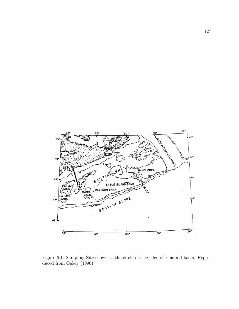
127
Figure 6.1: Sampling Site shown as the circle on the edge of Emerald basin. Repro-duced from Oakey (1990)

128
will be is called a sequence in this chapter. The 190 profile locations are shown in
Figure 6.2.
The dissipation data were obtained using direct measurements of vertical shear
to dissipation scales averaged over vertical bins of approximately 3.4 m using the
EPSONDE profiler. Temperature was also recorded by EPSONDE at approximately
2 cm intervals, although a version of the data with 40 cm intervals is used here.
The advantage of this data is that dissipation and temperature are measured from
the same instrument. If the instrument falls through a dissipative overturning event
then both the dissipation and the APEF should be high. If the sensors were not on the
same vehicle, many profiles would have to be averaged together to allow comparisons
between dissipation and finestructure because different profilers would not likely pass
through exactly the same mixing and finestructure conditions. Another advantage
is that dissipation is measured directly; in Dillon’s data, dissipation was obtained
indirectly from the temperature spectra using the Batchelor method.
It is unfortunate that the best data set available was not used for this chapter
as data with 2 cm resolution exists (versus 40 cm used here). Data were obtained
second-hand and this resulted in my misunderstanding of the full data set. Sooner
presentation of my results to the principal investigator, Neil Oakey, would have re-
sulted in an earlier detection of this. Data analyses were completed with the alternate
data set before I learned that a better data set existed. In particular, dissipation of
temperature variance (χθ) data are available, taken simultaneously with ǫ data used
here. I was not aware of this. Future analyses of that data could be done to infer the
dissipation of potential energy and compare it directly with the overturning models
two and three for buoyancy flux. This would yield a much better comparison than
the one presented here against ǫ only, where the two models cannot be differentiated.
The interpretation of the data set is thus not without problems. The temperature
sampling interval of 40 cm is large to sample overturns; however, the largest overturns
found are many meters in size such that they are still well resolved. Overturn detection
is theoretically limited to those bigger than the sampling interval, but in practice it

129
Figure 6.2: EPSONDE Sampling Stations. In all, 190 profiles of good quality weremade. Line are bathymetry at 10 m interval, starting with 100 m at the upper leftcorner to 210 m at the lower right.

130
is preferable to resolve an overturn with many points. This is both to assure that the
overturn is real, and to reduce the error in evaluating APEF. Also, the temperature
least count is 0.001◦C (the instrument resolution is 0.0015◦C; data were saved with
0.001◦C least count), which is not over-sampled, such that there are few noise-related
inversions (although the temperature gradient data from EPSONDE has much greater
resolution than this). This may sound good, but it prevents the use of a statistical
method, briefly described in appendix D, to determine the temperature sensor noise
level. These two factors, instrument least count and especially sampling interval,
combine to make the noise level of the finestructure-estimated buoyancy flux very
high, especially in high stratification (this will be quantified later).
6.2 T–S Characteristics
When temperature is re-ordered to find overturns, it is assumed that temperature
inversions are not salinity-compensated. The T–S relation of the water column be-
comes a very important tool to determine the presence of salinity-stabilized inversions
and intrusions.
The water column in Emerald basin (as everywhere else on the shelf, the Gulf
of St. Lawrence and up into the estuary) is characterised by salinity monotonically
increasing with depth, and by a mid-depth temperature minimum. CTD casts made
during the cruise have a temperature minimum of 4.5◦C between 30 to 50 m depth
(not shown). EPSONDE profiles are recorded from about 8 m below the surface to
the bottom, but will only be shown here below 60 m to compare with temperature
data below the temperature minimum.
The temperature at 60 m is always below the temperature minimum such that
temperature usually increases with depth and the salinity gradient controls the den-
sity gradient. Thus, instead of worrying about unstable temperature inversions being
compensated-for by salinity, a harder assumption must be made. Since the temper-
ature gradient is by itself statically unstable, it must be assumed that an overturn

131
appears as a stable temperature gradient, yet statically unstable because of an un-
measured salinity gradient.
To make this assumption, a one-to-one relation is required between temperature
and density. The relation does not need to be linear, but it must be tight, so that
temperature differences can be interpreted as density differences.
The T–S characteristics were not available from the EPSONDE profiler1 but CTD
casts were made before and after each sequence of profiles for the first half of the cruise
(until winch problems prevented CTD sampling). Figure 6.3 shows the T–S diagram
obtained from all the CTD data available from the cruise (taken over 4 days, with 2
days of overlap with the EPSONDE data). At first inspection, the T–S is straight
although it is wide. This presents a problem in the interpretation because the slope
of the main T–S line is close to isopycnal: an isopycnal line intersects with a range
of ≈ 0.15 ◦C in temperature due to the scatter of the T–S line. This means that
temperature inversions up to 0.15 ◦C observed within the scatter may be isopycnal
changes instead of diapycnal. There is thus danger that intrusions will be mistaken
as overturns. Still, no obvious deformations of the T–S line are observed, so we will
proceed, using temperature as a surrogate for density in our overturn detection.
6.3 Temperature Noise Level
The APEF is calculated by re-ordering the temperature profile obtained from EP-
SONDE (density was not measured). However, some of the temperature inversions
may be created by noise. In order to discard these overturns from the comparison,
and also to determine the noise level of the estimated buoyancy flux, the noise level
of the temperature sensor must be estimated.
A new technique for doing so is described in appendix D. Unfortunately, the
technique relies on having over-resolved temperature measurements such that noise
1Temperature and conductivity were both measured from EPSONDE, but an apparent calibrationproblem gave a T –S curve in disagreement with the CTD. T –S gradients have not been explored(Oakey, Pers. Communication).

132
33.0 33.5 34.0 34.5 35.0S (PSU)
4.0
6.0
8.0
10.0
T (
° C)
25.50 26.00 26.50 27.00
27.50
Figure 6.3: T–S diagram for all CTD data available from the cruise. In all 34445points from 66 profiles are shown. Isopycnals σt = 25.5 to 28.0 are indicated.

133
creates inversions, which are then separated from overturning signatures using run-
length statistics. The technique cannot be used with the current 40 cm sampling and
0.001◦C least count data.
While the same CTD used here but with a lower least count and finer vertical
sampling would probably yield a lower noise level, a conservative stance is taken and
the noise level is estimated as δT = 0.003◦C (3 times the least count). Overturns with
rms Thorpe fluctuations less than that are rejected. Further, overturns consisting of
3 points or less are also rejected.
6.4 Results
In chapter 3, buoyancy flux models were derived relating the decay of the APEF, ξ,
over a time scale of N−1 on one hand, and a decay time function of the turbulent
Froude number, Frt, on the other. The Frt-dependent decay time is shorter than
N−1 when there is much more turbulent kinetic energy than potential energy in the
turbulence (TKE ≫ 3ξ).
Since I have compared overturning measurements to ǫ instead of directly to χθ, it
is not possible to verify the buoyancy flux estimates. Therefore Jb will be estimated as
ξN , the upper bound of model three prediction (3.33), but the the lower Jb estimate
between model two and three at high Turbulent Froude number. Diagrams of ξN
versus ǫ will be shown, on which the ratio of ξN/ǫ is inferred as representing both
the mixing efficiency of model three and an indicator of Frt for model two. From
Frt = Ri−1/2t and (3.22), the turbulent Froude number is
Frt =
[
ǫ
2 ξ N
Lh
LT
]1/3
(6.1)
Note that this assumes ξ = N2L2T /2 (e.g. (2.28)). This approximation did not hold
for Dillon’s tabulated data (in chapter 5) because his layer averages were shown to
overestimate N2 within overturns, but it is expected to hold here because the density
gradient is evaluated separately over the depth interval of each overturn.

134
A given ξN/ǫ ratio implies two different values of Frt (or Rit) depending on the
assumption made for the unknown value of Lh in (6.1). In model two, isotropy sets
Lh = LT such that the Lh/LT ratio cancels out, leaving
(Frt)iso =
[
ǫ
2 ξ N
]1/3
(6.2)
In model three, inertial-buoyancy balance sets Lh = LO. The Lh/LT ratio becomes
LO/LT which can be written (ǫ/2ξN)1/2 (again using ξ = N2L2T /2). Thus, if inertial-
buoyancy balance conditions of model three hold, the relation between Frt and ξN/ǫ
becomes
(Frt)IB =
[
ǫ
2 ξ N
]1/2
(6.3)
Values of ξN/ǫ correspond directly to the mixing efficiency of the third model,
Γ3 = ξN/ǫ (from Jb = ξ N and Γ = Jb/ǫ). From (6.2) and (6.3), a given value of ξN/ǫ
(or Γ3) corresponds to different values of Frt at isotropy and inertial-buoyancy balance
such that (Frt)iso = (Frt)2/3IB
2. Since efficiencies in both models are proportional to
Rit (or Fr−2t ), the mixing efficiency of model two can be obtained from ξN/ǫ (or Γ3)
as
Γ2 =23ξ N (Frt)iso
ǫ=
1
3
[
2ξ N
ǫ
]2/3
≈ 0.53
[
ξ N
ǫ
]2/3
(6.4)
by noting that Jb = (2/3)ξNFrt in model two.
The mixing efficiency of the second model can thus be obtained directly from the
mixing efficiency of the third model for given values of ξN/ǫ on plots of ξN versus ǫ.
Mixing efficiencies for both models will be presented on a single ξN versus ǫ diagram.
6.4.1 Expected Outcome
The expected outcome is a good correlation between ξN and ǫ if at isotropic inertial-
buoyancy balance (where Frt ≈ 1), and ξN ≪ ǫ in well mixed layers or growing
turbulence (where Frt ≫ 1). Since the measurements were taken to the bottom
2This discussion is identical to the general form of Rit = (L2
T /L4/3
O L2/3
h ) in terms of length scalesbeing written as either (Rit)iso = (LT /LO)4/3 or (Rit)IB = (LT /LO)2.

135
where mixing is expected to be more intense, it is likely that some well-mixed layers
will be sampled and that a mix of conditions will be found. The ξN versus ǫ diagram
should then resemble the L2T N3 versus ǫ panel in Figure 5.2.
6.4.2 Data Sub-set—Sequence 10
The finestructure data is first compared to microstructure for the sequence of EP-
SONDE drops numbers 10018 to 10026. Ship drift was slow during this sequence.
The temperature field and a qualitative comparison between TKE dissipation and ξN
for overturns are shown in Figure 6.4 where the gray scale represents ǫ and the boxes
represent overturns; the depth span of the boxes coincides with the overturn sizes,
and the half-widths are values of ξN evaluated over distinct overturns. The depth
span of an overturn is defined as the smallest group of consecutive points which may
be re-ordered without moving any other point in the profile.
While qualitative agreement is found between high levels of ǫ and ξN , there are
very few overturns in regions of high temperature gradients, especially in the 60–90 m
range. The noise level for ξN (not shown) affects how much finestructure should
be found, and will be shown to be responsible for these quiet areas (where ǫ is low
anyway). Note that I do not have temperature profiles down to the bottom coinciding
with the lower-right region of high dissipation, so that the absence of overturns is not
a failure of the models.
6.4.3 Finestructure Noise Level
The noise level for Jb = ξN is determined by the minimum resolvable ξ and the value
of N . Recall that the APEF noise level was discussed in chapter 2; it is the higher of
the two values from (2.33). In this case, temperature is translated to density using
δρ = 0.12 δt, so ∂ρo/∂z = 0.12 ∂To/∂z, where the gradient of the re-ordered profile is
calculated by centered first-difference over an interval of ± 4 data points.
Temperature, dissipation, ξN and the noise level of ξN profiles are shown in
Figure 6.5 for sequence 10018–10026. Dissipation should only be compared with the

136
40 45 50 55 60 65 70 75 80 85time (min) starting day 286 at 08:39
160
140
120
100
80
60
40 45 50 55 60 65 70 75 80 85time (min) starting day 286 at 08:39
160
140
120
100
80
60
5
6
7
8
9
10000 series10-8 10-6
ξ N (W kg-1)
18 19 20 21 23 24 25 26
Figure 6.4: EPSONDE 10018 to 10026 sequence are qualitatively compared withoverturning events and isotherms. The contours show the temperature field. Thegray scale represents ǫ with white equal to 10−9 W kg−1 and black equal to 3.1 ×10⁻⁷ W kg−1. Each box identifies an overturn: the vertical extent of the box showsthe vertical extent of the overturn and the half-width of the box represents the valueof ξN of the overturn from the scale on the upper left. Thus, a half-width of zero cmon the page means that ξN < 10−9 W kg−1.

137
estimated buoyancy flux ξN in depth intervals where dissipation is greater than the
buoyancy flux noise level. This is the least severe criterion that can be applied because
the mixing efficiency is expected to be less than unity. In a mixed layer of high Frt,
the mixing efficiency is expected to be much lower, say 0.1. In this case the buoyancy
flux would be 10 times lower and dissipation should only be compared to ξN where
the noise level is 10 times lower than ǫ.
The determination of the temperature noise level is therefore important because it
determines the fraction of the water column in which buoyancy flux should be resolved
by the finestructure. Note that since the ξN noise level increases with stratification
(See Figure 6.5) finestructure cannot resolve overturning in the thermocline above
90 m or so, where no overturns are observed in Figure 6.4.
6.4.4 Averaging in 10-m Bins
The finestructure and microstructure for sequence 10018–10026 are averaged in 10 m
bins in Figure 6.6. Values of ξN are plotted only for bins in which ξN is higher than
the noise level. Note that the averages are of ξN , using N and ξ within each overturn;
values of N are not 10-m averages in this case.
By comparing Figures 6.5 and 6.6, it is seen that most energetic overturns have
thickness scales of the order of the bin size (10 m), such that the bin-averaging ξN
does not affect their values. The averaging affects ǫ much more, removing many high
wavenumber variations.
There are 49 10-m bins for which ǫ is greater than the ξN noise level. The average
mixing efficiency Γ3 for these 49 bins, calculated as the average ratio of ξN/ǫ, is 0.69
(corresponding to Γ2 = 0.51). There are 43 bins for which ǫ times 0.69 (representing
an average buoyancy flux) is greater than the noise level of ξN , the buoyancy flux for
model three; perhaps this better represents the number of bins (43) in which values
of ξN greater than noise level are expected to be measured. However, there are only
17 10-m bins for which ξN is greater than its noise level, compared to the expected
number of 43. Thus the distribution of resolved buoyancy flux by overturning is

138
160
140
120
100
80
60
160
150
140
130
120
110
100
90
80
70
60
10023 10024 10025 10026
160
150
140
130
120
110
100
90
80
70
60
10018
10-9 10-8 10-7 10-6
(W kg-1)
4 6 8 10T (°C)
10019
10-9 10-8 10-7 10-6
(W kg-1)
4 6 8 10T (°C)
10020
10-9 10-8 10-7 10-6
(W kg-1)
4 6 8 10T (°C)
10021
10-9 10-8 10-7 10-6
(W kg-1)
4 6 8 10T (°C)
Figure 6.5: Noise level for ξN in 10018–10026 sequence. The thick gray line is thenoise level for ξN . The thick black line is ǫ. Overturns are not expected to be observedif ǫ is less than the noise level. The black rectangles span the depth of overturns andtheir width represents ξN for the overturn. These quantities are on a logarithmicscale of 10−9 to 10−6 W kg−1. The temperature profile is also plotted (thin line).

139
160
140
120
100
80
60
160
150
140
130
120
110
100
90
80
70
60
10023 10024 10025 10026
160
150
140
130
120
110
100
90
80
70
60
10018
10-9 10-8 10-7 10-6
10019
10-9 10-8 10-7 10-6
10020
10-9 10-8 10-7 10-6
10021
10-9 10-8 10-7 10-6
Figure 6.6: Averages in 10 m bins for ξN and ǫ in 10018–10026 sequence. The thickgray line is the noise level for ξN and the thick black line is ǫ. Symbols are averagedvalues of ξN for each 10 m bin, and are only plotted if greater than the noise level ofthe bin. All quantities are on a scale of 10−9 to 10−6 W kg−1.

140
lower than expected from TKE dissipation rate measurements; overturning (and its
modelled buoyancy flux) is found only in about 40% of the 10 m bins in which it
should be resolved.
In Figure 6.7, ξN is plotted against ǫ for both overturn values of Figure 6.5 and
averages of Figure 6.6. For Figure 6.7, overturn values for dissipation are simply
the average ǫ measured within the span of the overturn. Only overturns consisting
of more than 3 points and with rms Thorpe fluctuations greater than 0.003◦C are
shown. If the overturn does not vertically overlap with any dissipation sample point,
it is compared to the closest dissipation measurement (so it is only an average for
large overturns, greater than about 3.4 m).
While the ξN versus ǫ distributions in Figure 6.7 are slightly different for the
averaged and non-averaged cases, it is difficult to say if 10-m averaging is necessarily
better than taking overturn values, having no other estimates of buoyancy flux to
compare with (from χθ, for example). It is clear that the overturn-averages do not
yield results dramatically different from 10-m averages; this is probably due to the
fact that most energetic overturns have length scales similar to 10 m. This large size
would not be true of Dillon’s observations discussed in chapter 5.
6.4.5 Analysis on Entire Data Set
Here, the above comparison is repeated on the entire data set. In Figure 6.8, ξN
is compared to ǫ for each overturn in the data set resolved by more than 3 data
points and for which T ′21/2> 0.003◦C. A plot showing the same result in terms of
ξ1/2N−1 vs LO is also shown (where multiplying ξ1/2N−1 by 21/2 approximates LT )
because LT –LO diagrams are often seen in the literature to compare finestructure to
dissipation.
Obviously, the comparison is not very good when all data are considered in the plot
of ξN versus ǫ. The expected result is similar to Figure 6.7, where points of maximum
ξN for all ǫ values falls along a line of constant mixing efficiency Γ = ξN/ǫ. The cloud
of data below this line is expected for well mixed layers or intense, growing turbulence

141
10-9
10-8
10-7
10-6
ξ N
(W
kg-1
)
10-9 10-8 10-7 10-6
ε (W kg-1)
Γ3 = 1Γ2 = 0.53
Γ3 = 0.1Γ2 = 0.11
Figure 6.7: Buoyancy flux estimate ξN versus dissipation ǫ in 10018–10026 sequence.The dots are averages over the span of each overturn (from Figure 6.5). Only overturnsconsisting of more than 3 points and with rms Thorpe fluctuations greater than0.003◦C are shown. The circles are 10-m bin averages (from Figure 6.6). Only binswith ξN greater than noise level are shown. The oblique lines are mixing efficiencieswith the indicated values for the second and third models.

142
Γ3 = 1Γ2 = 0.53
Γ3 = 0.1Γ2 = 0.11
10-9 10-8 10-7 10-6
ε (W kg-1)
10-9
10-8
10-7
10-6
ξ N
(W
kg-1
)
C - All data
Γ3 = 1Γ2 = 0.53
Γ3 = 0.1Γ2 = 0.11
10-9 10-8 10-7 10-6
ε (W kg-1)
D - Selected data
10-1 1 101
Lo (m)
10-1
1
101
ξ1/2 /N
(m
)
A - All data
10-1 1 101
Lo (m)
B - Selected data
Figure 6.8: Buoyancy flux estimate ξN versus dissipation ǫ, and ξ1/2N−1 vs LO fordepth spans of well-resolved overturns, for all data set. In A and C, all data areplotted but are coded as: (+) shallower than 65 m; (◦) between 8.6 and 9◦C. Dotsare all other data. In B and D, only dots from A and C are plotted (deeper than 65 m,
yet not between 8.6 and 9◦C). These well resolved data are have T ′21/2> 0.003◦C
and more than 3 points per overturn. Note that ξ1/2N−1 approximates 0.707 LT . Theoblique line in A and B is a one-to-one line. The oblique lines in C and D are mixingefficiencies with the indicated values for the second and third models.

143
where high Frt turbulence has low mixing efficiency. The data with high value of ξN
and low values of ǫ are ‘anomalous’ in the models. We will use this qualifier for now
to designate them because the models cannot account for mixing efficiencies much
greater than unity.
It is found that most of these ‘anomalous’ data are selected using two criteria. The
first group are between 60 and 75 m, but have no special temperature other than they
usually fall within 4 to 7◦C. The second group are in the temperature range of 8.6 to
9◦C. These data are removed in Figure 6.8B and D. The result is much better, more
like Figure 6.7 with a triangle of values with ǫ ≫ ξN allowed (low mixing efficiency)
but not the reverse. This ‘filter’ is to say the least Ad Hoc; it is only used now as a
signature to help determine what is different about these selected data. This will be
examined later in this chapter.
6.5 Discussion
Let us now review what this data analysis has revealed about the unanswered ques-
tions enumerated at the beginning of the chapter.
6.5.1 Does Averaging Over Single Overturns Compare Well
With 10-m Averages?
The comparison of ξN and ǫ yield slightly different results in Figures 6.7. The biggest
difference observed is an apparent decrease in dissipation variance with depth (seen
mostly by comparing Figure 6.5 to Figure 6.6).
Here, we would ideally wish to compare estimates of the buoyancy flux obtained
from overturning to the true buoyancy flux within the overturn, in order to estimate
the importance of the redistribution terms of kinetic and potential energy in the
governing turbulent equations. But we do not know the true buoyancy flux, nor
even an estimate (although further work could use χθ measurements). We have a
measurement of the rate of dissipation of TKE from single profiles, for which the

144
same redistribution terms usually force us to ensemble average many profiles. The
best that can thus be done is to see if estimates of buoyancy flux from single overturns
are as consistent with the dissipation of TKE averaged over those overturns, as they
are using larger scale 10-m averaging.
The averaging on 10-m bin is typical of what is usually done. For instance,
Dillon’s (1982) data are for mixing layers which may hold many overturns. A major
difference remains: the finestructure buoyancy flux models were not evaluated here
by using a layer-averaged N , but rather with an N evaluated over each overturn and
then averaged. The bias introduced in Dillon’s analysis is not present here. Here,
N is calculated by regression on the re-ordered temperature profile over the span of
each individual overturn.
It is encouraging that the results are not dramatically different than those using 10-
m bin averaging, however it must be noted that most of the more energetic overturns
are of this size anyway, such that 10-m averaging should not be expected to be
dramatically different.
Note that it is not known if the overturns are evolving K-H billows (puffs). over-
turning may be occurring in more persistent mixing layers such that initial overturning
with high ξ but little ǫ (which could be observed in K-H billows) is not expected. This
is because the shear forcing is likely to be steady in the boundary layer, as evidenced
by many subsequent profiles with overturning near the bottom.
6.5.2 How Much of the Rate of Dissipation of TKE is Ac-
counted for by Overturning?
If the mean mixing efficiency (for sequence 10018–10026) of Γ3 = 0.69 is used, then
it could be assumed that bins with ǫ greater than 0.69 times the buoyancy flux noise
level should contain resolved overturns. Only 40 percent of them do. In particular,
station 10023 has a high dissipation relative to buoyancy flux noise level for 10-m
averages, and yet has very little overturning. If the expected mean mixing efficiency
is reduced by half to 0.35, then 60 percent of the bins where overturns are expected

145
to be resolved do contain overturns.
Note that the average mixing efficiency is biased because not all bins have over-
turns, and those without overturns were not included in the calculation of mixing
efficiency. Therefore, that number should not be used outside of the loose context in
which it was introduced.
It is unclear why overturns are not observed in many of the bins for which overturn-
ing is expected. An hypothesis is that mixing efficiency is very low where overturns
were not observed, such that overturning is below the noise level. This cannot be
tested without estimates of Frt or measurements of χθ. However, Figure 6.7 shows
that the highest ξN/ǫ ratio, occurring consistently at all values of ǫ, has a value
greater than unity, corresponding to a high maximum mixing efficiency in models
two and three (the higher still values of ξN/ǫ which occur only at low values of ǫ will
be discussed separately). This perplexing result could be an averaging problem, or
partly due to a changing T–S water mass line changing the conversion from temper-
ature difference to density difference3. Note that such high mixing efficiencies were
also observed in Dillon’s data set, but that I have argued that they might be due
to errors in χθ. Therefore, it seems unlikely that very low mixing efficiency occurs
adjacent to very high values.
Thus, no clear answer to this question may be given here.
6.5.3 How Much of the Overturning is Accounted for by the
Rate of Dissipation of TKE?
If overturning is observed (and models consequently predict high buoyancy flux) when
the rate of dissipation of TKE is low and cannot account for any buoyancy flux,
this would not be seen in comparisons done using only data where both ǫ was well
resolved and overturning occurred (e.g. Dillon’s analysis). The present data have
3Because the T –S line is fairly close to isopycnal, small differences could account for large changes.Up to a 30% reduction in the temperature to density conversion results in changing from the mainT –S line to a secondary line shown in upcoming Figure 6.10

146
such occurrences. In the next section, I will try to convince the reader that these are
intrusions and not overturning events; they should therefore be discounted from the
comparison with the rate of dissipation of TKE. The presence of intrusions is in fact
the major difficulty with the interpretation of this data, and possibly many data sets
with energetic mixing.
6.6 Intrusions and Water Masses
The main problem with the interpretation of the data are those ‘overturns’ with very
high ξN and very low rates of dissipation of TKE. Most of these anomalous data were
found to be either between the depths of 60 and 75 m or between the temperature of
8.6 and 9.0◦C.
The two groups of anomalously high ξN data are not spread about equally in
all the data set. Figure 6.9 shows the overturn-averaged ξN versus ǫ for each time
sequence of EPSONDE drops from the drifting ship. Note that not all sequences
suffer from these points, and those that do often have many such points (which are
spread over many profiles).
The T–S properties of the CTD data are re-examined in Figure 6.3 to identify
what is different about the data between 60 and 75 m and also about those between
8.6 and 9.0◦C. Upon close inspection, one can discern different water masses in
Figure 6.3. In Figure 6.10, two water mass families are shown which appear to be
the extremes found in the CTD data. It is possible, and likely, that these two water
masses may interleave and also mix together since both these masses were sampled
in close proximity.
CTD casts were taken between EPSONDE sequences for the first part of the
cruise (until they experienced winch problems). There are two sequences for which
CTD data is available which have anomalous ξ data characterised by 8.6–9.0◦C water.
These are stations 13 and 14, and the T–S diagrams are shown in Figure 6.11. It is
seen that sampling in stations 13 and 14 started in one water mass and finished in

147
10-9
10-8
10-7
10-6
10-5
ξ N
(W
kg-1
)
10-9 10-8 10-7 10-6 10-5
ε (W kg-1)
4
10-9
10-8
10-7
10-6
10-5
ξ N
(W
kg-1
)
5
10-9
10-8
10-7
10-6
10-5
ξ N
(W
kg-1
)
6
10-9
10-8
10-7
10-6
10-5
ξ N
(W
kg-1
)
8
10-9
10-8
10-7
10-6
10-5
ξ N
(W
kg-1
)
10-9 10-8 10-7 10-6 10-5
ε (W kg-1)
9
10-9 10-8 10-7 10-6 10-5
ε (W kg-1)
10
11
13
14
10-9 10-8 10-7 10-6 10-5
ε (W kg-1)
15
10-9 10-8 10-7 10-6 10-5
ε (W kg-1)
16
17
18
20
10-9 10-8 10-7 10-6 10-5
ε (W kg-1)
21
10-9 10-8 10-7 10-6 10-5
ε (W kg-1)
10-9
10-8
10-7
10-6
10-5
ξ N
(W
kg-1
)
22
10-9
10-8
10-7
10-6
10-5
ξ N
(W
kg-1
)
23
10-9
10-8
10-7
10-6
10-5
ξ N
(W
kg-1
)
10-9 10-8 10-7 10-6 10-5
ε (W kg-1)
25
Figure 6.9: Overturn-averages of ξN vs ǫ for individual EPSONDE sequences. (+)shallower than 65 m; (◦) between 8.6 and 9◦C; (2) all other data. Sequence numberindicated in upper left corner of each panel. Oblique line is mixing efficiency Γ2 = 0.53or Γ3 = 1.

148
33.0 33.5 34.0 34.5 35.0S (PSU)
4.0
6.0
8.0
10.0
T (
° C)
25.50 26.00 26.50 27.00
27.50
Figure 6.10: Water masses found on T–S relation. The two lines represent the extremewater masses found on the T–S relation in Figure 6.3.

149
the other. The temperature at the intersection of these two water masses is in the
range of the observed high ξN (8.6–9.0◦C). Possibly, an intrusion was occurring close
to the intersection temperature of the two water masses.
The EPSONDE data characterised by depths between 60 and 75 m (‘plus’ symbols
on Figure 6.9) cannot be found on all T–S diagrams of Figure 6.11 made from CTD
casts. For example, T–S diagrams for sequences 6 and 9 are not shallow enough to
observe characteristics found in this depth range (although this is merely due to a
cut-off depth chosen for the CTD files given to me because the region of interest was
the bottom boundary layer (Van Haren, Pers. Communication)). For this reason,
we will again look to EPSONDE station 14 to explain the high ξN found in depths
between 60 and 75 m (Different points within the profiles than those found between
8.6 and 9.0◦C).
In sequence 14, there is a possibility that a mixture of both water masses in
Figure 6.10 is intruding along an isopycnal into the sampling drift track. This stable
intrusion has a different temperature for its density than would otherwise be seen.
When EPSONDE enters or leaves the intrusion, the the temperature gradient would
reverse and create an apparent overturn.
Figure 6.12 shows the drift track of sequence 14, as well as the positions of the pre-
ceeding and following CTD casts. The time evolution is also shown, with time against
the latitude position. The drift and sampling were fairly regular. Supported by this,
the temperature at a chosen isopycnal is plotted linearly between the preceeding and
following CTD cast position in the third panel of Figure 6.12. The temperature was
observed to decrease by 0.5◦C at that isopycnal during the time span of the sequence,
from 7.1 to 6.6◦C (in less than 6 hours). The ‘overturns’ with high ξN centered
between 60 and 65 m (for this sequence, generally these points are between 60 and
75 m) are only found during the first five stations of sequence 14. They are shown as
black dots in Figure 6.12. The minimum and maximum temperatures for each of the
‘overturns’ are connected and shown in the third panel. They show that the decrease
in temperature of that ‘overturn’ throughout the sequence of profiles is consistent

150
4
6
8
10
T
33 34 35S
4
4
6
8
10
T
5
4
6
8
10
T
6
4
6
8
10
T
7
4
6
8
10
T
33 34 35S
9
33 34 35S
10
11
13
33 34 35S
14
Figure 6.11: T–S diagram for all EPSONDE sequences preceeded and followed by aCTD cast. The two lines are water masses traced on Figure 6.10. Sequence numberindicated in upper left corner of each panel. Note that the finestructure density mea-surements in these CTD casts is unreliable; none of the apparent density inversionsshould be believed. In certains sequences, two end water masses are found at the startand end, such that intrusions could be present during the sequence. These intrusions,not observed in any way in this figure, could be seen as overturns by EPSONDE usingonly temperature profiles.

151
with the observed temperature decrease at an isopycnal going through the ‘overturn’.
This suggests that the ‘overturns’ are in fact temperature signatures of an intrusion
of both end water masses.
The origin of the mixed intrusion is unclear. It occurs at the same depth, yet
different temperatures, in many profiles. In particular sequence 6 has an apparent
intrusion at the same depth, but this time between 4 and 5◦C instead of around 7◦C.
Through 6 consecutive profiles, the intrusion temperature decreases by 0.6◦C. There
are no sills at a depth of 60 to 70 m close by. The closest is Emerald bank, 70 to
80 m in depth, at over 20 km away from these stations.
6.7 Summary
In this chapter, microstructure data from Emerald Basin were used as a test case of the
finestructure models for estimating buoyancy flux from overturns. The temperature
data used have low vertical resolution for overturn detection (40 cm resolution was
used here, but 2 cm resolution data exist) and so areas of high stratification were not
resolved by the method. However, overturning was often on such large vertical scales
(≈ 10 m) that even the 40 cm vertical sampling resolves them easily.
The main results were
• The buoyancy fluxes obtained from the overturn finestructure were consistent
with the dissipation measurements even if data are averaged over the vertical
extent of separate overturns (See Figure 6.5 and Figure 6.7). To my knowledge,
this is the first time that these quantities have been compared on such small
averaging spans. However, the large overturning size limits the applicability of
this result to less energetic mixing layers.
• About 40 to 60% of 10-m bins in which overturning was expected were observed
to contain overturns.
• The maximum mixing efficiency observed is fairly high (Γ3 ≈ 2). Low mixing
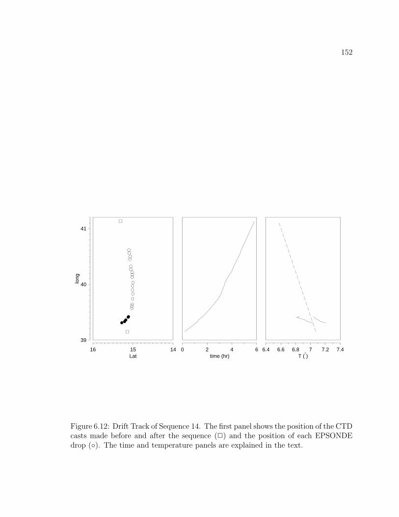
152
39
40
41
long
16 15 14Lat
0 2 4 6time (hr)
6.4 6.6 6.8 7 7.2 7.4T (°)
Figure 6.12: Drift Track of Sequence 14. The first panel shows the position of the CTDcasts made before and after the sequence (2) and the position of each EPSONDEdrop (◦). The time and temperature panels are explained in the text.

153
efficiencies were Γ3 < 0.1 using the third model (or Γ2 < 0.04 using the second
model). Note that these mixing efficiencies come from buoyancy flux models
using the upper bound of the factor of two of their coefficient ([
34± 1
4
]
). Re-
gardless of this factor, there is a range of about 2 decades in observed mixing
efficiency (not counting bins where no overturns were observed), but the instru-
ment resolution limits this range. This implies that the data are incompatible
with model one, which assuming a constant mixing efficiency. The same was
said of Dillon’s data sets A and C.
• Temperature was used as a density tracer to identify and compute the potential
energy of the overturning events. A tight T–S relation is required for this to
work properly. In regions where ξN was much higher than ǫ, it was shown
that the sequence started in one water mass and finished in another. Persistent
apparent overturns warmed from profile to profile consistently with isopycnal
changes between the two end water masses. This strongly suggests that the
high ξN anomalies were in fact intrusions.
• This is perhaps the most important point: If dissipation data had not been
available, and only finestructure were used to estimate mixing, all data where
the T–S varied greatly would not be used because of the possibility of misin-
terpreting intrusions as overturns. It is therefore recommended that salinity
always be measured if it can affect density in a significant amount. Even if den-
sity measurements cannot resolve overturning events sufficiently to reorder the
profiles to find overturns, it is probably good enough to help identify inversions
caused by intrusions. These often have uncommonly high values of ξN .
Chapter 7
Application to the St. Lawrence
Estuary
Microstructure measurements have yet to be taken in the St. Lawrence estuary, yet
many authors have discussed the strong mixing that occurs at the head of the Lau-
rentian channel (Steven, 1974; Forrester, 1974; Ingram, 1975; Therriault and Lacroix,
1976; El-Sabh, 1979; Gagnon and El-Sabh, 1980; Ingram, 1983). It is thought that
mixing occurs predominantly at the head of the channel (Steven, 1974), and that
large shears associated with an internal tide provide the forcing (Forrester, 1974).
This internal tide appears to be generated at the slope where bathymetry shallows
from 350 m to 50 m in less than 15 km (Forrester, 1974), but the exact mechanism
is not confirmed1
In this chapter, CTD and ADCP data sampled at the head of the channel are
used in conjunction with the buoyancy flux models discussed in this thesis to estimate
mixing rates.
1While it can be argued that a critical slope at the head can reflect some tidal energy and createthe internal wave, at least one author has proposed otherwise. Blackford (1978) constructed a 2-layer generation model without rotation whereby continuity dictates that the flow over the sill mustbe greater than seaward. A Bernoulli depression over the sill accelerates the flow by generating apressure gradient in the surface layer. Since there is no flow in the bottom layer seaward of the sill,the interface must tilt to compensate the pressure gradient in the top layer. The periodic tidal flowover the sill thus creates a wave at the interface which propagates seawards.
154

155
This chapter serves three purposes. First, it illustrates what is known about the
hydrodynamic conditions in the area, hopefully adding to that knowledge and iden-
tifying some weak points. This includes discussions of the internal tides, intrusions
and solitons. Second, an attempt is made to quantify mixing, to show what forces
it, and to determine its range of turbulent Froude number Frt. The Froude number
will be estimated from the larger scale gradient Richardson number Rig. No further
comparison can be made between mixing models presented in earlier chapters because
microstructure quantities (ǫ, χθ) were not measured here. Third, the overturning will
be related to the shear forcing by comparison with Gregg’s (1989) model which links
shear to dissipation levels.
7.1 CTD and ADCP Data Set
During a preliminary cruise on the Petrel V in the fall of 1987, density inversions
thought to be overturning events were measured using a conventional GuildLine CTD.
A longer, second cruise took place in late June of 1988 on the C.S.S. L.-M. Lauzier.
During the last three days of the cruise, an R&D Instruments 1200-KHz ADCP was
graciously lent to us for demonstration purposes by David Stewart of Dasco Equip-
ment Inc. The ADCP sampled velocity vectors in 1-m bins and 2-minute averages
from 3 to 32 m. The velocities are measured relative to the surface bin because the
sea floor was beyond the bottom-tracking range of the ADCP.
7.1.1 Gradient Richardson Numbers
The gradient Richardson number, Rig, is an indicator of the dynamic stability of the
water column. It has been shown to be related to the turbulent Froude number, Frt,
in a previous chapter, by
Fr−2t = Rit ≈ 6.2 Rig (7.1)
However, gradient Richardson numbers can be evaluated at different vertical scales.
A brief outline of the methodology used for this data set follows.
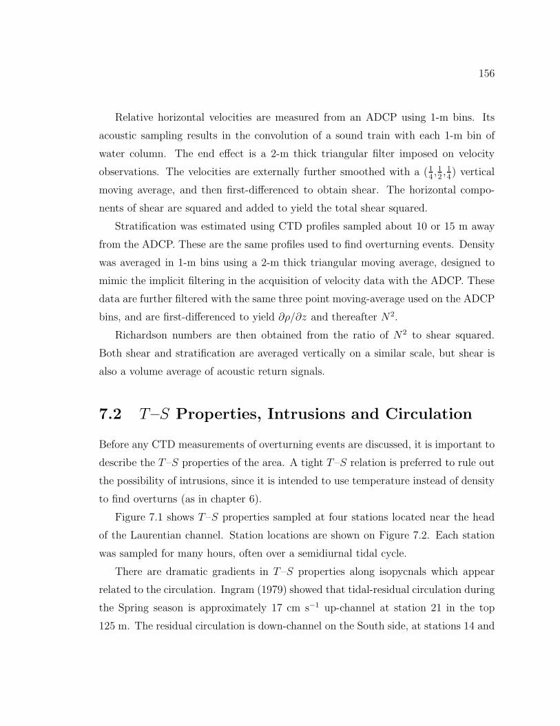
156
Relative horizontal velocities are measured from an ADCP using 1-m bins. Its
acoustic sampling results in the convolution of a sound train with each 1-m bin of
water column. The end effect is a 2-m thick triangular filter imposed on velocity
observations. The velocities are externally further smoothed with a (14,12,14) vertical
moving average, and then first-differenced to obtain shear. The horizontal compo-
nents of shear are squared and added to yield the total shear squared.
Stratification was estimated using CTD profiles sampled about 10 or 15 m away
from the ADCP. These are the same profiles used to find overturning events. Density
was averaged in 1-m bins using a 2-m thick triangular moving average, designed to
mimic the implicit filtering in the acquisition of velocity data with the ADCP. These
data are further filtered with the same three point moving-average used on the ADCP
bins, and are first-differenced to yield ∂ρ/∂z and thereafter N2.
Richardson numbers are then obtained from the ratio of N2 to shear squared.
Both shear and stratification are averaged vertically on a similar scale, but shear is
also a volume average of acoustic return signals.
7.2 T–S Properties, Intrusions and Circulation
Before any CTD measurements of overturning events are discussed, it is important to
describe the T–S properties of the area. A tight T–S relation is preferred to rule out
the possibility of intrusions, since it is intended to use temperature instead of density
to find overturns (as in chapter 6).
Figure 7.1 shows T–S properties sampled at four stations located near the head
of the Laurentian channel. Station locations are shown on Figure 7.2. Each station
was sampled for many hours, often over a semidiurnal tidal cycle.
There are dramatic gradients in T–S properties along isopycnals which appear
related to the circulation. Ingram (1979) showed that tidal-residual circulation during
the Spring season is approximately 17 cm s−1 up-channel at station 21 in the top
125 m. The residual circulation is down-channel on the South side, at stations 14 and

157
0
2
4
6
8
10
T
24 26 28 30 32 34 36S
24
24 26 28 30 32 34 36S
21
14
0
2
4
6
8
10
T
11
Figure 7.1: Temperature–Salinity Properties at the head of the Laurentian channel.Stations indicated in upper-right corner of each panel. Station locations are shown inFigure 7.2. Station 21 was sampled to 200 m every hour starting June 27 1988 15:01EDT to June 28 04:58 EDT. Station 24 was also sampled to 200 m every hour, onJune 29 from 14:01 to 22:59 EDT; Winds increased from very low to 25 knots at theend of the day. Station 14 was sampled to 50 m on July 4 from 04:50 to 14:04 EDTin 15 knot winds. Station 11 to 50 m was sampled from July 4 14:57 to July 5 02:45in light winds. The last 3 profiles were taken to 235 m. See text for explanation ofwater mass lines.

158
Figure 7.2: Study area in the Lower St. Lawrence estuary. Adapted from In-gram (1979).

159
24.
The V-shaped solid lines added to Figure 7.1 indicate the main water masses
found, except for some surface cooling at stations 21 and 24, and surface warming
at station 11 and, to a lesser extend, station 14. The deepest waters have a uniform
T–S distribution for all stations. The T–S relation above the temperature minimum
is tightest for Station 11 and 21, consistent with advection of undisturbed water into
what is assumed to be a stronger mixing region.
Ingram (1979) found that the temperature minimum increased by less than 1◦C
between May 1973 at Gaspe and July 1973 near station 21. This 3-month inter-
val corresponds to the advection time between the two locations. He used a sim-
ple advection-diffusion model of the temperature minimum to estimate mixing along
the Laurentian channel. He could explain half of the temperature change by using
Kρ∂2T/∂z2 = 10−7◦C s−1 and Kρ = 2 × 10⁻⁵ m2 s−1. Ingram obtained these mixing
rates from internal tide modes (Forrester, 1974) and an eddy diffusivity parameteri-
zation in term of the gradient Richardson number (Jones, 1973).
Since the minimum temperature at station 24 varies by more than 1◦C, it is
noteworthy that 3 months of diffusion along the Laurentian channel is overwhelmed
within a time which could be presumed to be a few tidal cycles at most. This is
presumed to occur here because of the larger internal tides combined with the poorly
understood circulation at the slope of the head of the channel, or between the channel
and the South bank of the lower estuary. Water masses which do not usually come into
contact probably meet, and their mixing results in the various water masses forming
the temperature minimum at station 24. Several profiles at station 24 contained
intrusions between the two end water masses between σt = 24 and σt = 26.
All profiles at station 14 have an anomalous water mass corresponding to the
dashed line shown on Figure 7.1. The water mass ends on its dense side with an
isopycnal intrusion around σt = 25. If the water mass is extended to σt = 26, it
corresponds more or less to the upper temperature minimum of station 24. Thus the
end points of this water mass could be at σt = 22 and σt ≈ 26 on the main T–S lines

160
described by the ‘V’.
The water mass on the dashed line is usually found on the South side of the
channel, where circulation is down-channel. However, it appears at lower densities at
station 11 some of the time.
The intrusions might result from ‘horizontal’ spreading of mixed layers formed
by mixing light waters with dense water heaved over the sill by the large isopycnal
displacement of the internal tide. The intrusions provide clues to the circulation and
mixing at the head of the channel; they also complicate the sampling of overturning
events. It would be preferable to use temperature alone from the CTD to identity
overturns because temperature is easier to measure accurately within overturns than
density (e.g. one sensor instead of combining both temperature and conductivity
within the enhanced gradients of overturns). It is possible to use temperature alone
for most of the profiles of station 11 where the T–S relation is very tight. Yet in
many cases intrusions can be falsely interpreted as overturns. The combined use of
conductivity and temperature in the demanding environment of overturns must then
be used if overturns are to be identified. In known intrusions, no attempt will be
made to identify any overturns.
7.3 Internal Tide Description
If the mixing at the head of the channel is thought to be forced mostly by the shear
associated with the internal tide, then analytic expressions of the internal tide could
potentially be used to compare expected Rig to observed Rig and overturning events,
and to fill the gaps where and when no data were taken.
In this section, I will briefly discuss how my observations differ from the literature
on the internal tide, and why using previous results and analytical expressions of the
internal tide have very limited application in predicting mixing. Work presented here
is by no means the final word, but should serve as a useful guide for future work.

161
Forrester (1974) provided a description of the internal tide in the Laurentian chan-
nel from current-meter measurements from nine moorings, located from the head of
the channel to over 100 km toward the mouth of the estuary. He fitted the observa-
tions to modes associated with internal Kelvin and Poincare modes of various tidal
frequencies, obtaining the vertical modal structure from a mean density profile. Data
were consistent with an internal Poincare wave in the second vertical mode (one zero-
crossing of isopycnal displacements at 72 m; the first vertical mode is evanescent in
a 25 km channel width using Forrester’s density profile) and first lateral mode, at
frequency M2 and wavelength of 60 km, propagating toward the Gulf in a channel of
320 m depth and 25 km width. Forrester also found some evidence for the presence of
a Kelvin wave at diurnal frequency, also propagating out of the estuary. Since most
of the energy is found at semidiurnal frequency in the lower estuary, the Poincare
mode is addressed specifically here.
This section will address the following points:
• Effect of the mean density profile on modal shapes, showing that small changes
in the profile lead to different modal shapes (mostly in the depth of the node
for the second vertical mode).
• Comparison of two possible modal shapes with data, showing that an alternate
choice than Forrester’s leads to a more representative node depth for the second
vertical mode.
• Restrictions on vertical modes from channel width, due to the dispersion rela-
tion, showing that the channel may be too narrow at the head to support the
second vertical mode, even though it is observed.
• Comparison of observed shears to second vertical mode, showing that the vari-
ability of the shears could not be adequately modelled as simple internal tides
to obtain analytical forms for Rig to compare against observed mixing. The
observed shear will thus be compared to mixing, but no attempt will be made

162
to use analytical forms of Rig to predict where mixing should occur, and how
much it should mix.
7.3.1 Mean Density Profile in Present Data Set—Effect on
Modal Shape
In Forrester (1974), the mean density profile was approximated by the wholly empir-
ical formula
ρ(z) = ρoe−a/(z+b) (7.2)
where ρo was set to 1028 kg m−3, a = 0.2016 m and b = 29.29 m.
This density profile yielded the vertical modes of the wave, η(z), as the eigenfunc-
tions of
ηzz +
[
N2 − ω2
c2n
]
η = 0 (7.3)
where η is isopycnal displacement, subscript z indicates differentiation with respect
to z, N2 is the stability—a function of ρ(z)—and ω is the wave frequency (M2 tidal).
Application of the surface and bottom boundary conditions η(0) = η(H) = 0 to
the solution of (7.3), neglecting ω2 with respect to N2, sets the eigenvalues cn for the
n vertical modes of oscillation.
Figure 7.3A compares the density profile chosen by Forrester to profiles of the
present data set at stations 21 and 24, covering about a tidal cycle at each station.
The stations are located on either side of the channel (see Figure 7.2). Water on
the North side is saltier then on the South side because of the sideways estuarine
circulation. Flow on the North side is mostly up the estuary, and barely reverses on
ebb flow. The fresher outflow is mostly restricted to the South side.
Figure 7.3B shows the rms difference in density between observations and the
best fitting profiles for various values of a and b (choosing ρo at each a–b pair to
minimize the difference). Forrester’s choice is shown with a dot, as well as an alternate
choice at a = 0.03 m, b = 2 m. While Forrester’s choice results in slightly less
error, and arguably a much better fit at depth (See panel A), the alternate choice

163
18 20 22 24 26 28σT
250
240
230
220
210
200
190
180
170
160
150
140
130
120
110
100
90
80
70
60
50
40
30
20
10
0D
epth
(m
)
A Forrester’s fit
a = 0.03b = 2
1
1
2
5
5 10 15 20 25 30b
0.05
0.1
0.15
0.2
0.25
a
B
75
50
25
0
Depth (m
)
C
H = 250 m
H = 320 m
η(z)
D
250
200
150
100
50
0
Depth (m
)
U(z)
E
Figure 7.3: Mean density profile and its effect on node depth. A- Observed densityprofiles over nearly a tidal cycle at station 21 (solid) and 24 (dash) compared toForrester’s fit and an alternate fit; B- rms difference between observations and bestfitting density profiles of a–b pairs. Dots shows a–b values for profiles in A; C-Depth of node of the second vertical mode for a channel of depth 320 m (thick) and250 m (thin) as function of b; D- Eigenfunction for isopycnal displacements, η, of thesecond vertical mode for Forrester’s fit (thick) and b = 2 m (thin); E- Eigenfunctionfor velocity, dη/dz, of the second vertical mode for Forrester’s fit (thick) and b = 2 m(thin).

164
perhaps approximates the steppiness of shallow observations better, although only
very crudely with a sharper pycnocline. Forrester’s choice may be a smoothed best
fit to an average that is never observed2. In any case, the selection of a mean profile
is not very sensitive to the parameter b.
In panel C, the depth of the node of the second vertical mode is shown. It depends
only on the parameter b and the depth of the channel. Forrester used a depth of 320 m,
suitable for the channel as a whole; A curve for H = 250 m is also shown because
it is more representative of the depth at our stations near the head of the channel.
Note that Forrester’s density profile results in a node at 72 m in a channel of 320 m
depth. The node is much shallower (20 m) for b = 2, with not much dependence on
the depth of the channel.
In panels D and E, the vertical modes for isopycnal displacements (D) and ve-
locity (E) are shown for both b = 29.29 m (thick line) and b = 2 m (thin line). In
conclusion to Figure 7.3, very different vertical modes are obtained with two mean
density profiles of slightly different errors with respect to observations. Forrester’s
mean profile may thus lead to wrong modes. The alternate choice for b will be shown
shortly to qualitatively better match observations. Perhaps future work should select
modes by fitting to isopycnal displacements rather than to density profiles.
7.3.2 Comparison of Modal Shapes With Present Data Set
Figure 7.4A shows isopycnal displacements for station 21 and 24 versus tidal phase
(same data as in Figure 7.3A). Sampling at station 24 started 47 hours after sampling
commenced at station 21, but the data are plotted versus barotropic tidal phase such
that they can be compared, with Station 24 repeated. In panel B, the isopycnal
displacements predicted from b = 2 m in Figure 7.3D are shown for comparison.
There appears to be a phase lag with depth of the observed isopycnal motions,
with deeper isopycnals moving later. More importantly, there is no node at 72 m as
2The time-average at every depth is influenced by the heaving due to the internal tide, becausethis motion was not removed before the mean density profile before it was fitted

165
250
200
150
100
50
0
Dep
th (
m)
H L H L
B
250
200
150
100
50
0
Dep
th (
m)
A 21 ∆H = 1.8 m ∆H = 2.8 m ∆H = 3.1 mSurf elev: 24∆H = 2.3 m ∆H = 2.3 m
27
26
25
24232221 20
26.5
2727
26
25242322
26.5
Figure 7.4: A- Isopycnal displacements for station 21 (thin line) and 24 (thick line)vs tidal phase. Station 24 is shown twice to better compare it with station 21. Thetidal elevations indicated are surface elevation differences between high and low tides.High tide is indicated by H, low tide by L; B- Theoretical isopycnal oscillations forthe second vertical mode with density profile described by (7.2) with b = 2 m. Thephase with respect to the barotropic tide is not determined, and can be offset in panelA. The inversions on both series at high tide is due to overturning in both cases.

166
Forrester’s fit predicted. On the data shown here, there is only a hint of isopycnal
motion near the surface to indicate whether the second mode exists at all. If it does,
its node is much shallower that predicted by Forrester (See also Figure 7.7B for a
more evident node at 20 m at station 11). It appears that the modes obtained using
a = 0.03 m and b = 2 m represent our data better than those chosen by Forrester.
7.3.3 Restrictions on Vertical Modes And Along-Channel
Structure of the Internal tide
The non-uniformity of the channel brings about a problem when the possibility of
existence of various vertical modes is considered. The dispersion relation for Poincare
waves in the nth vertical mode and mth lateral mode is
k2nm =
ω2 − f 2
c2n
− λ2m (7.4)
where knm is the along-channel wavenumber, f is the Coriolis parameter and λm =
mπ/W is the cross-channel wavenumber in a channel of width W .
Forrester used an average channel width of W = 25 km. Substituting this value
into (7.4), the first vertical mode is not possible because k11 is imaginary. Thus
Forrester looked for a fit against the second and higher modes. However, setting
W to the channel width at the head of the channel, approximately 7.5 km, makes λ1
increase over 3-fold. In this case, only the sixth and higher vertical modes are possible
in this linear theory. Obviously, the observed isopycnal motions in Figure 7.4A are
not in such a high mode.
An imaginary wavenumber translates to a non-propagating wave with an along-
channel decay length-scale of k−1: an evanescent mode. The wavenumber, describing
a propagating or evanescent wave, can be explored for various values of a and b.
Substituting the density profile (7.2) into the governing equation (7.3), and using the
boundary conditions η(0) = η(H) = 0, the following expression for cn is obtained
c2n =
ga
14
+[
nπln((H+b)/b)
]2 (7.5)
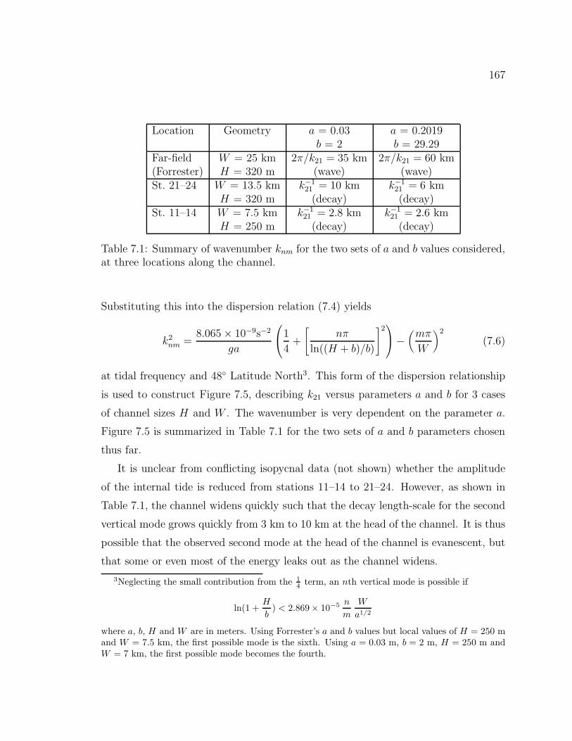
167
Location Geometry a = 0.03 a = 0.2019b = 2 b = 29.29
Far-field W = 25 km 2π/k21 = 35 km 2π/k21 = 60 km(Forrester) H = 320 m (wave) (wave)St. 21–24 W = 13.5 km k−1
21 = 10 km k−121 = 6 km
H = 320 m (decay) (decay)St. 11–14 W = 7.5 km k−1
21 = 2.8 km k−121 = 2.6 km
H = 250 m (decay) (decay)
Table 7.1: Summary of wavenumber knm for the two sets of a and b values considered,at three locations along the channel.
Substituting this into the dispersion relation (7.4) yields
k2nm =
8.065 × 10⁻⁹s−2
ga
1
4+
[
nπ
ln((H + b)/b)
]2
−(
mπ
W
)2
(7.6)
at tidal frequency and 48◦ Latitude North3. This form of the dispersion relationship
is used to construct Figure 7.5, describing k21 versus parameters a and b for 3 cases
of channel sizes H and W . The wavenumber is very dependent on the parameter a.
Figure 7.5 is summarized in Table 7.1 for the two sets of a and b parameters chosen
thus far.
It is unclear from conflicting isopycnal data (not shown) whether the amplitude
of the internal tide is reduced from stations 11–14 to 21–24. However, as shown in
Table 7.1, the channel widens quickly such that the decay length-scale for the second
vertical mode grows quickly from 3 km to 10 km at the head of the channel. It is thus
possible that the observed second mode at the head of the channel is evanescent, but
that some or even most of the energy leaks out as the channel widens.
3Neglecting the small contribution from the 1
4term, an nth vertical mode is possible if
ln(1 +H
b) < 2.869× 10⁻⁵
n
m
W
a1/2
where a, b, H and W are in meters. Using Forrester’s a and b values but local values of H = 250 mand W = 7.5 km, the first possible mode is the sixth. Using a = 0.03 m, b = 2 m, H = 250 m andW = 7 km, the first possible mode becomes the fourth.

168
C - Head of channel - St. 11 to 14
W = 7.5 km
H = 250 m
0-1
5 10 15 20 25 30b
0.05
0.10
0.15
0.20
0.25
a
B - 9 km from head of Channel - St. 21 to 24
W = 13.5 km
H = 320 m
0
-1
0.05
0.10
0.15
0.20
0.25
aA - Far from head of Channel - Forrester’s Geometry
W = 25 km
H = 320 m
0
0.05
0.10
0.15
0.20
0.25
a
Figure 7.5: Wavenumber k21 (×104) for various a and b values. Negative values—found above the zero line—are in fact imaginary (e-folding decay wavenumber). Dotsindicate both Forrester’s choice for a and b and the alternate choice with secondmode node depth of 20 m. A- W = 25 km and H = 320 m, corresponding to the farfield geometry of the channel used by Forrester; B- W = 13.5 km and H = 320 m,corresponding to the channel geometry at stations 21–24; C- W = 7.5 km and H =250 m, corresponding to the channel geometry at stations 11–14.
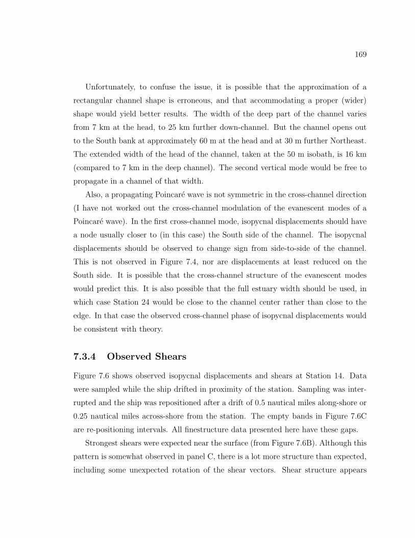
169
Unfortunately, to confuse the issue, it is possible that the approximation of a
rectangular channel shape is erroneous, and that accommodating a proper (wider)
shape would yield better results. The width of the deep part of the channel varies
from 7 km at the head, to 25 km further down-channel. But the channel opens out
to the South bank at approximately 60 m at the head and at 30 m further Northeast.
The extended width of the head of the channel, taken at the 50 m isobath, is 16 km
(compared to 7 km in the deep channel). The second vertical mode would be free to
propagate in a channel of that width.
Also, a propagating Poincare wave is not symmetric in the cross-channel direction
(I have not worked out the cross-channel modulation of the evanescent modes of a
Poincare wave). In the first cross-channel mode, isopycnal displacements should have
a node usually closer to (in this case) the South side of the channel. The isopycnal
displacements should be observed to change sign from side-to-side of the channel.
This is not observed in Figure 7.4, nor are displacements at least reduced on the
South side. It is possible that the cross-channel structure of the evanescent modes
would predict this. It is also possible that the full estuary width should be used, in
which case Station 24 would be close to the channel center rather than close to the
edge. In that case the observed cross-channel phase of isopycnal displacements would
be consistent with theory.
7.3.4 Observed Shears
Figure 7.6 shows observed isopycnal displacements and shears at Station 14. Data
were sampled while the ship drifted in proximity of the station. Sampling was inter-
rupted and the ship was repositioned after a drift of 0.5 nautical miles along-shore or
0.25 nautical miles across-shore from the station. The empty bands in Figure 7.6C
are re-positioning intervals. All finestructure data presented here have these gaps.
Strongest shears were expected near the surface (from Figure 7.6B). Although this
pattern is somewhat observed in panel C, there is a lot more structure than expected,
including some unexpected rotation of the shear vectors. Shear structure appears

170
layered along isopycnals (panel D). The average of the surface density slice is taken
in panel E (σt < 21) and a shear vector rotating clockwise at tidal frequency provides
an adequate fit, as seen by low residuals of unorganized patterns in panel F. Note that
along and cross-channel components of shear were independently fitted for phase and
amplitude; both were fitted best with the same phase, such that the shear ellipse is
aligned along the axis of the channel. The fitted near-surface clockwise-rotating shear
vector is consistent with a Poincare wave. Its phase is along-channel simultaneously
with maximum isopycnal displacements (near high tide, indicated with an ‘H’ between
panels A and C). This is also consistent with a Poincare internal tide anywhere across
the channel, with the possibility of a sign change of the shear.
While some of the observed shear seems consistent with a Poincare internal tide,
the cross-channel modulation was not compared to theory, nor were amplitudes (be-
cause of the evanescent mode). Some of the shear variability does not compare well
with predictions in panel B. There is no reason to believe that observed gradient
Richardson numbers should compare well to those predicted from theoretical shears
and the idealized density profile. Even if the onset of mixing could be predicted,
theory would then have to account for the density profile evolving into layers.
7.3.5 Summary of the Internal Tide
In this section, it was observed that
• Forrester’s mean density profile does not match the large gradients near the
surface.
• A wide range of analytical density profiles with various parameters a and b in
(7.2) can fit observations with similar errors.
• The depth of the node of the second vertical mode depends greatly on b. It is
at 72 m for Forrester’s profile (b = 29.29), and at 20 m for b = 2.
• Isopycnal displacements at Stations 21 and 24 are consistent with b = 2, rather
than with b = 29.29.

171
50
40
30
20
10
0
Dep
th (
m)
A
CH L
B
26
25
24
23
22
21
20
19
σ t
D
0 0.1 0.2s-1
10
5
0
Dep
th
E
10
5
Dep
th
60 120 180 240 300 360 420 480 540 600time (min) starting 04 Jul 88 04:54:39 EDT
F
Figure 7.6: Shear and isopycnal displacements at Station 14. A- Isopycnal displace-ment obtained from CTD casts sampled approximately every 4 minutes, collected atthe same time as the shear vectors of panel C; B- Theoretical Poincare shear depth-modulation for n = 2, b = 2 m and H = 250 m; C- Shear vectors from 0 to 32 m.Towards the right is down-channel and downwards is toward the South side of thechannel. Scale indicated in panel D; D- Shear plotted against density; E- Bottomarrows: average shear for σt < 21. Top arrows: Tidal-frequency rotating vector least-squares fit to bottom arrows; F- Difference between average shear and fit in panel E;Boxed areas in A and C indicate mixing layers described in later sections. Letters Hand L between panels A and C indicate high and low tide.

172
• The observed second mode may be evanescent at the head of the channel due
to the narrow width of the deep channel. The e-folding distance varies quickly
from 3 km to 10 km between stations 14 and 11, less than 10 km apart. Thus
large shears measured at the head may only be typical at the head due to a
non-propagating wave. Alternatively, the second mode is free to propagate if
the full width of the estuary is used instead of the deeper Laurentian channel.
• Surface shears are consistent with a Poincare internal tide at tidal frequency
(M2), but there are some inconsistent deeper large shears that seem homoge-
neous in isopycnal layers.
These observations add to the body of knowledge of the internal tide at the head
of the Laurentian channel. They also raise questions that future investigators should
consider. Modal fits are not a viable solution to predicting mixing because of the
variability of the shear and of stratification so that Rig cannot be modelled well
by a simple analytical form, and because of the effect of mixing itself on the shear
and density profile. The internal tide must be considered as a measured but mostly
unpredicted forcing, and go on from there to compare it with observed overturning.
It is unclear if mixing rates measured here will be applicable to areas further down-
channel because it is uncertain if measured shears are representative of down-channel
forcing (evanescent or propagating wave?). The mixing area could be limited to only
a few kilometers from the head, or it could extend further down-channel.
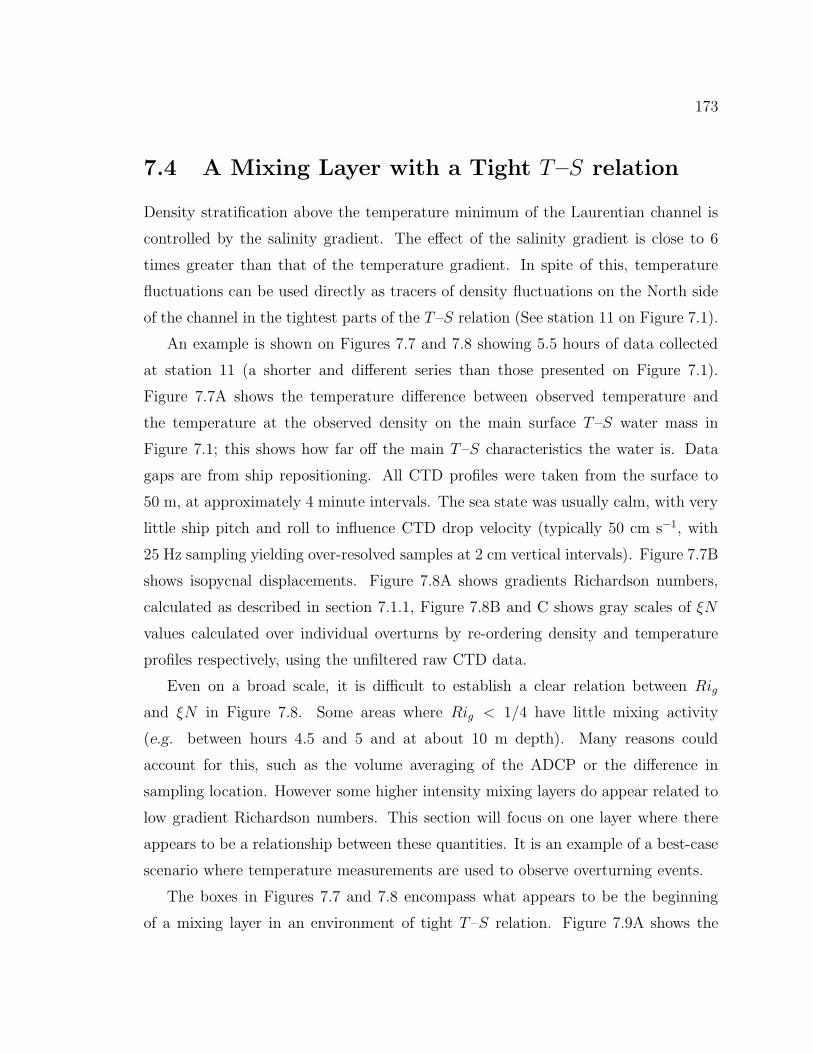
173
7.4 A Mixing Layer with a Tight T–S relation
Density stratification above the temperature minimum of the Laurentian channel is
controlled by the salinity gradient. The effect of the salinity gradient is close to 6
times greater than that of the temperature gradient. In spite of this, temperature
fluctuations can be used directly as tracers of density fluctuations on the North side
of the channel in the tightest parts of the T–S relation (See station 11 on Figure 7.1).
An example is shown on Figures 7.7 and 7.8 showing 5.5 hours of data collected
at station 11 (a shorter and different series than those presented on Figure 7.1).
Figure 7.7A shows the temperature difference between observed temperature and
the temperature at the observed density on the main surface T–S water mass in
Figure 7.1; this shows how far off the main T–S characteristics the water is. Data
gaps are from ship repositioning. All CTD profiles were taken from the surface to
50 m, at approximately 4 minute intervals. The sea state was usually calm, with very
little ship pitch and roll to influence CTD drop velocity (typically 50 cm s−1, with
25 Hz sampling yielding over-resolved samples at 2 cm vertical intervals). Figure 7.7B
shows isopycnal displacements. Figure 7.8A shows gradients Richardson numbers,
calculated as described in section 7.1.1, Figure 7.8B and C shows gray scales of ξN
values calculated over individual overturns by re-ordering density and temperature
profiles respectively, using the unfiltered raw CTD data.
Even on a broad scale, it is difficult to establish a clear relation between Rig
and ξN in Figure 7.8. Some areas where Rig < 1/4 have little mixing activity
(e.g. between hours 4.5 and 5 and at about 10 m depth). Many reasons could
account for this, such as the volume averaging of the ADCP or the difference in
sampling location. However some higher intensity mixing layers do appear related to
low gradient Richardson numbers. This section will focus on one layer where there
appears to be a relationship between these quantities. It is an example of a best-case
scenario where temperature measurements are used to observe overturning events.
The boxes in Figures 7.7 and 7.8 encompass what appears to be the beginning
of a mixing layer in an environment of tight T–S relation. Figure 7.9A shows the

174
2 3 4 5 6 7time (hours) starting July 3rd 1988
50
40
30
20
10
0
Dep
th
B
20
21222324
25
50
40
30
20
10
0D
epth
0
0
0
0
0
0
0
0
0
0
0
0
0
-0.2
-0.2-0.2
-0.2
-0.4
-0.4
-0.4
-0.4
A011-1
Figure 7.7: Isopycnal displacements and temperature anomaly at station 11. A-Temperature anomaly versus depth, where temperature anomaly is defined as T =37.284−1.445 σt, the difference between observed temperature and that calculated forobserved σt from least-squares fit between 0 and 6 ◦C for station 011 on Figure 7.1;B- Isopycnal displacements; The box indicates a mixing layer discussed in the text.The gaps in A are due to ship repositioning; contours are constructed from verticalprofiles typically separated by 4 minutes in time.

175
2 3 4 5 6 7time (hours) starting July 3rd 1988
30
25
20
15
10
5
Dep
th
C - ξ N from T
30
25
20
15
10
5
Dep
th
B - ξ N from σt
30
25
20
15
10
5D
epth
A - Ri011-1
Figure 7.8: A- Gradient Richardson numbers at station 11. Black on white contourline is for Rig = 10, shaded areas for Rig < 1 and white on black contour is forRig = 1/4; B- Quantity ξN calculated for each overturn measured using density.Only overturns with rms ρ′ > 0.005 kg m−3 are shown. Gray scale is log-linear from10−8 W kg−1 (white) to 10−4 W kg−1 (black); C- ξN calculated for each overturnmeasured using temperature as density tracer. Gray scale same as B. The box onall panels indicates a mixing layer discussed in the text. The gaps correspond tosampling interruption due to ship repositioning.

176
10 temperature profiles in this patch. Notice the richness in finestructure in the first
few profiles compared to the last. This could suggest the evolution of a mixed layer,
but the difference in velocity between 3 m and 12 m is of order 15 cm s−1, and is
up to 45 cm s−1 between 3 m and 22 m (velocities are not shown). These velocities
translate to an advection distance of ≈ 400 m and ≈ 1250 m between the ship and the
top and bottom of the layer during the 46 minute time span of the sampling. Thus
an energy budget would require assumptions about the horizontal structure and will
not be pursued here.
Only temperature profiles are shown in Figure 7.9A but density profiles would be
fairly close to mirror images. The tight T–S relation in Figure 7.9B shows this. As
a further example, Figure 7.9C shows the T–S relation for a part of the first profile
shown in Figure 7.9A. There are several overturns with temperature excursions of 0.1
◦C which are difficult to see because their deviations from the main T -S line are small
(more about this below). As a consequence, temperature inversions can be related to
density inversions by a proportionality constant which includes both temperature and
salinity effects in density. Figure 7.8 shows both ξN calculated using temperature
and density fluctuations.
The T–S characteristics of Figure 7.9C can be related to the measurements of
an overturn with a ‘perfect‘ CTD. Assuming that the T–S relation is linear in the
water column, then a CTD sampling overturned water will record T and S on the
same T–S line as would were the water not overturning. If only points are plotted,
a T–S diagram from a perfect CTD would show nothing out of the ordinary. If the
measurements are connected by a line, then that line should oscillate between denser
and lighter waters found within the overturn on the T–S diagram. This resembles
what is seen in Figure 7.9C, with very little deviation off of the main T–S line.
When deviations are found, they can be due to enhanced temperature and salinity
gradients within the overturn highlighting any sensor mismatch between temperature
and conductivity sensors. If the deviations are isopycnal, rather than on the main
T–S line, then it is likely that an isopycnal water intrusion was measured rather than

177
6 7 8T (°C)
23
22
21
20
19
18
17
16
15
14
13
Dep
th
A
26 27S (PSU)
6
7
8
T (
° C)
B
26.8 27 27.2 27.4 27.6S (PSU)
6
6.2
6.4
6.6
6.8
7
T (
° C)
C
Figure 7.9: A- Temperature profiles for the 10 profiles of the mixing layer at station 11discussed in the text and shown in the box in Figure 7.7. Only down traces of theCTD profiles are used. The profiles are shown alternatively with thin and thick lineto better identify them; B- T–S diagram for the same 10 profiles; C- T–S diagramfor part of the first profile. Note the tight relation even within overturning events.

178
an overturn.
7.4.1 Mixing Rates
Forty-three percent of the length of the profiles in Figure 7.9A is overturning. The
average value of Jb = ξN for the layer is 3.4 × 10⁻⁷ W kg−1. Difficulties arise
when evaluating a value of the turbulent Froude number to yield an estimate of
buoyancy flux from the isotropic growing turbulence model using Jb = (2/3) ξNFrt.
Since the eye picks up some correspondence between ξN and Rig in Figure 7.8,
some sort of patch averaging seems most appropriate for that layer, if somewhat
arbitrary. Values of ξN and Rig were time-averaged for the 46-minute time span
in each 1-m bin, and averages of ξN were further filtered with a (14,12,14) vertical
moving average as Rig was in the processing of N2 and shear-squared. The layer-
average value of Jb = (2/3)ξNFrt ≈ (2/3)ξN (0.4 Ri−1/2g ) is 1.2×10⁻⁷ W kg−1, using
(7.1) to relate Frt to Rig. However, if the minimum Rig in each 1-m 45-minute
bin is used to estimate the Froude number, then the buoyancy flux is estimated as
1.8×10⁻⁷ W kg−1, 50% greater than by using a mean value of Rig. It could be argued
that the minimum Rig observed is dynamically more important than more average
because the overturning can be caused by the lowest Rig measured. This factor can
perhaps be used as a rough estimate of the error in Frt.
The average stratification in the layer is N2 = 10−3 s−2. Combined with the
buoyancy fluxes from both models two and three, this yields an eddy diffusivity of
Kρ = JbN−2 ≈ 1 to 3 × 10⁻⁴ m2 s−1 (Which model should be most suitable will be
discussed in section 7.7). Some averaging is required to compare this value to Ingram’s
mean value along the channel (Kρ = 2 × 10⁻⁵ m2 s−1). If only one such layer occurs
every tidal cycle, mixing for 40 minutes, then the time-averaged Kv would be 5.3% of
the layer Kρ. This is very similar to Ingram’s result of 2× 10⁻⁵ m2 s−1. Considering
that Ingram calculated the mixing of a layer (not the entire water column) due to
the mixing forcing of the internal tide, it seems reasonable to compare these time-
averaged values of Kρ. Since sampling was only for half a tidal cycle, and that a few

179
other mixing layers are observed in Figure 7.8, mixing is slightly more intense during
this 6-hour observation period at the head of the channel than the average mixing
further down the channel (assuming N2 is comparable in both cases such that Kρ is
an appropriate measure of mixing).
Of course, this is only the mixing from one of the patches on Figure 7.8, which
shows only one 6-hour observation. It cannot be assumed that this observation is
typical; a few more observations follow.
7.5 A Mixing Layer in a Loose T–S relation
In the previous section, a mixing layer with tight T–S was shown where temperature
inversions always correspond to overturning. In this section, a time-series from the
South side of the Laurentian channel is presented. It is used to demonstrate how
intrusive water masses are the main difficulty in identifying overturns with a CTD,
even when one uses density to find inversions.
Figures 7.10 and 7.11 show isopycnals, temperature anomaly, Richardson numbers
and the mixing parameter ξN for station 14, as Figures 7.7 and 7.8 did for station 11.
The data shown from station 14 is simultaneous with shear measurements shown
on Figure 7.6 and with the T–S diagram of station 14 on Figure 7.1. The warm
intrusion at σt ≈ 25 described in Section 7.2 and observed on Figure 7.1 is evident on
the temperature anomaly plot, rising to 30 m at 31 hours. The use of either density
or temperature from CTD measurements to identify overturns will not be attempted
within this feature. It will be shown here that more subtle T–S features, which are
not as evident, also cause problems.
The deep data gap in Figure 7.10A is caused by the processing cut-off of the
profiles at 0 ◦C, above the temperature minimum of the water column.

180
29 30 31 32 33 34 35 36 37 38time (hours) starting July 3rd 1988
50
40
30
20
10
0
Dep
th
B
20
21
22
23242526
50
40
30
20
10
0D
epth
1
0.8
0.80.8
0.8
0.6
0.6
0.6
0.60.6
0.6
0.6 0.6
0.6
0.4
0.40.4
0.4
0.4
0.40.4
0.4
0.4
0.2
0.20.2
0.2
0.2
0.2
0.20.2
0.20.2
0.2
0.2
0
0
0
0
A14
Figure 7.10: Isopycnal displacements and temperature anomaly at station 14. A-Temperature anomaly versus depth, where temperature anomaly is defined as T =37.2838−1.44494σt, the difference between observed temperature and that calculatedfor observed σt from least-squares fit between 0 and 6 ◦C for station 011 on Figure 7.1;B- Isopycnal displacements; The boxes indicate a mixing layer and soliton discussedin the text.
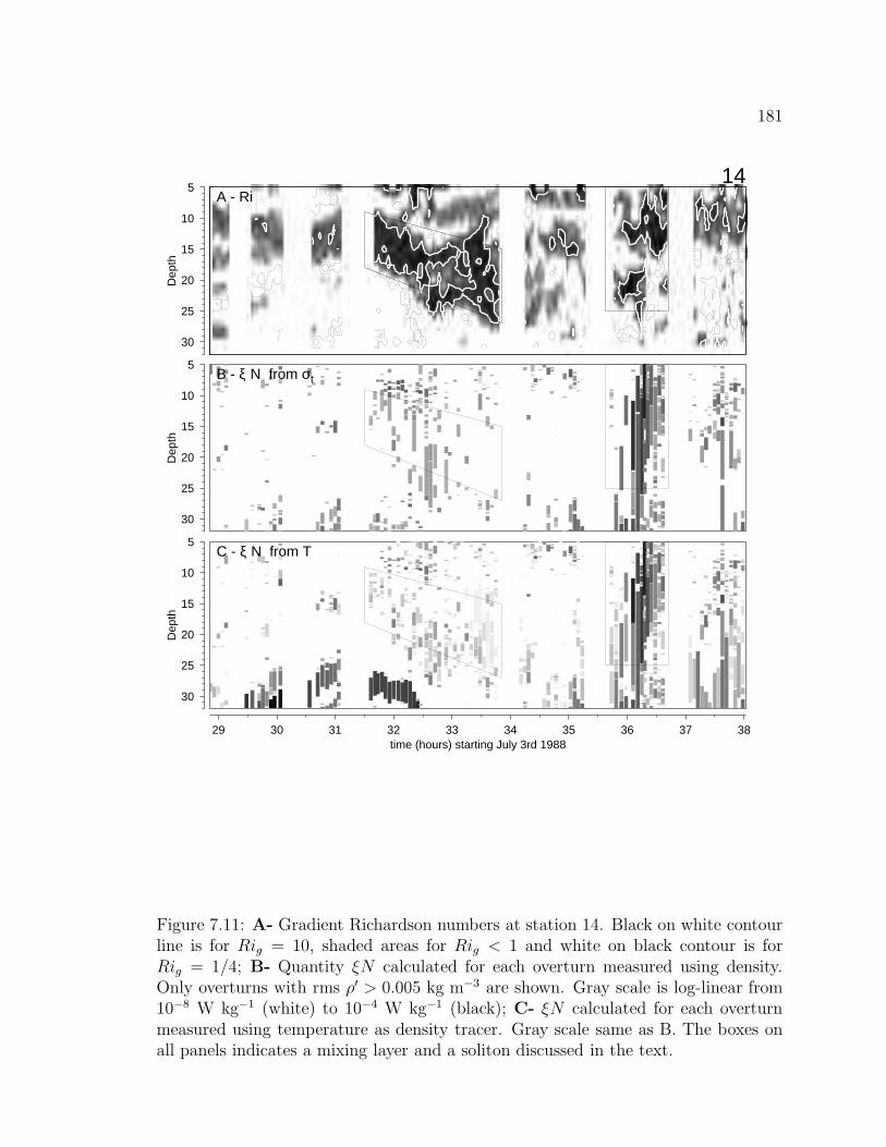
181
29 30 31 32 33 34 35 36 37 38time (hours) starting July 3rd 1988
30
25
20
15
10
5
Dep
th
C - ξ N from T
30
25
20
15
10
5
Dep
th
B - ξ N from σt
30
25
20
15
10
5D
epth
A - Ri14
Figure 7.11: A- Gradient Richardson numbers at station 14. Black on white contourline is for Rig = 10, shaded areas for Rig < 1 and white on black contour is forRig = 1/4; B- Quantity ξN calculated for each overturn measured using density.Only overturns with rms ρ′ > 0.005 kg m−3 are shown. Gray scale is log-linear from10−8 W kg−1 (white) to 10−4 W kg−1 (black); C- ξN calculated for each overturnmeasured using temperature as density tracer. Gray scale same as B. The boxes onall panels indicates a mixing layer and a soliton discussed in the text.

182
7.5.1 Intrusive Layers
The first striking feature on Figures 7.10 and 7.11 is the mixing layer shown boxed
between 31.7 and 33.7 hours, consisting of 31 CTD casts. Stratification is very low
for that depth range, gradient Richardson numbers are mostly below 14
and the layer
appears to be overturning throughout. Overturning energy, as measured by ξN , seems
rather low. Most of the overturns that occur near the end of the layer are not seen
by re-ordering on density because of the high density fluctuation threshold selected4
The density range within the first half of the layer is fairly constant, but the
layer gets denser during the second half (see Figure 7.10). The T–S relation of the
profile of the first half are shown in Figure 7.12A; the T–S relation of the second
half is denser and is therefore not in the same T–S parameter space. The water gets
progressively warmer with successive CTD casts in Figure 7.12A. It appear that a
family of water masses are present, each on a T–S line going from warm-fresh to
cold-salty. Within each casts, these water masses are seen intruding into each other.
However, the warm-salty to cold-fresh lines joining up these water masses do not lie
on isopycnals; the isopycnal for σt = 21.6 is shown on Figure 7.12B.
Figure 7.12A shows what appear to be intruding stratified water masses, with
the top water mass denser than the one underneath! Figure 7.12B illustrates this;
only parts of the T–S lines which are unstable in density are shown. Instabilities
correspond to overturns when they lie on a unique T–S water mass; in this case, it it
difficult to determine if these are sampling artifacts or real structure.
Temperature and Conductivity Sensor Mismatch
A possible explanation for the density inversions of Figure 7.12B is time-response
mismatch between the CTD conductivity and temperature sensors. This is known
4Only overturns with an rms density fluctuation of 0.005 kg m−3 or greater are shown. Perhapsthis limit could be lessened if density were calculated to a forth significant decimal place. Withthe current density values calculated to three significant decimals, it is difficult to establish a goodestimate of the noise level. I opted to err on the side of caution by select only overturns having anrms density fluctuation of 0.005 kg m−3 or greater.

183
5.7
5.8
5.9
6
6.1
6.2
6.3
6.4
6.5
6.6
6.7
6.8
T (
°C)
27.5 27.6 27.7 27.8S (PSU)
A
5.7
5.8
5.9
6
6.1
6.2
6.3
6.4
6.5
6.6
6.7
6.8
27.5 27.6 27.7 27.8S (PSU)
B
27.5 27.6 27.7 27.8S (PSU)
C
5.7
5.8
5.9
6
6.1
6.2
6.3
6.4
6.5
6.6
6.7
6.8
0.648 0.65 0.652 0.654 0.656 0.658Conductivity Ratio
D
Figure 7.12: A- T–S diagram for first 15 profiles of mixing layer described in text; B-T–S diagram showing only depth-spans where the density profile is statically unstable.Solid line is isopycnal for σt = 21.6; C- T–S diagram for right-most profile in A (dots).T–S lines offset to the left are obtained by using conductivity measurements offsetin depth with respect to temperature as explained in the text; D- Conductivity ratioversus temperature for profile in C (thick line) and its preceeding profile (thin line).

184
to result in what is commonly referred to as ‘spiking’. Such mismatch is discussed
in Perkin et al. (1982) and is summarized here. The 14 cm long conductivity cell
has approximately instantaneous response to new water when it has penetrated the
cell 7 mm past mid-point (although the response is to an average property of the
water found between the two electrode pairs, separated by 4 cm). The thermometer
is quoted as having a 50 ms response; its time response is said to be adequately rep-
resented by a simple exponential decay (Perkin and Lewis, 1982) if the drop speed is
held constant. At the descent rate of 50 cm s−1, this corresponds to a length-scale
of 2.5 cm. Since ship pitch and roll were minimal on our cruise, this representation
is thought to be adequate. Thus time-response mismatches could be reduced by cal-
culating salinity and density by combining conductivity with temperature measured
2 cm later, by which time the sensor has caught up with most of the temperature
changes as it can.
Figure 7.12C shows the right-most profile in Figure 7.12A and B with dots. Most
of the density inversions consist of many points and so cannot be dismissed as random
error. The profiles offset to the left are T–S calculated by offsetting temperature and
conductivity by 1 sample (≈ 2 cm), and then 2, and so on to 8 samples of offset.
This is much more than could be accounted for from the known sensor mismatch,
and none of these offsets resulted in eliminating—or even significantly reducing—the
density inversions.
Therefore, time-response mismatch of CTD sensors cannot account for the unusual
T–S structure observed in Figure 7.12A, at least using single-pole transfer functions
for the temperature sensor and instantaneous but delayed response of the conductivity
cell as suggested by Perkin et al. (1982).
Conductivity Cell Flushing
Another explanation for the density inversions of Figure 7.12B involves flushing of
the CTD conductivity cell. This is a narrow tube 14 cm long within which 2 electrode
pairs measuring conductivity are separated by 4 or 5 cm. It is conceivable that the

185
overturning circulation would be strong enough at low gradient Richardson numbers
(which is the case here) to prevent proper circulation through the conductivity cell.
However, I will show here that this is unlikely.
While is it true that turbulent velocities increase with decreasing values of Rig,
a brief look at Figures 7.10B and 7.6C indicates that low values of Rig must be
mostly due to low N2. Turbulent velocities are in fact proportional to the inverse of
the shear. From (7.1), the originating relation u′ = 0.4NLT Ri−1/2g is back-tracked.
Using Rig ≈ 0.15 and N2 in the range of 10−3 to 10−4 s−2, the turbulent velocity
is u′ ≈ (0.02s−1 ± 0.01)LT . Overturning scales would have to be about 10 m for
turbulent velocities to become comparable to the descent rate of the CTD instrument
of 50 cm s−1. Overturning scales are typically less than 1 m.
It is also not obvious that the turbulent velocity field preventing proper flushing
of the conductivity cell would result in the T–S characteristics of Figure 7.12A. The
conductivity ratio between in-situ water and standard sea-water is plotted versus
temperature in Figure 7.12D. The figure includes the profile shown in Figure 7.12C
and the preceeding profile. The curves have a stair-case shape, as might be expected
from interrupting the flushing of the conductivity cell. However, simultaneously with
conductivity remaining constant, temperature would be expected to quickly decrease
and then increase again if the sensor were going through an overturn. This expected
signature is not observed.
In summary, then, it remains a puzzle as to whether the density inversions ob-
served in Figure 7.12A are artifacts. A simple scheme of turbulent velocities associ-
ated with overturns inhibiting proper flushing of the conductivity cell cannot cause
mis-sampling similar to observations.
7.5.2 Mixing Rates
Density inversions found in this intrusive layer do not all occur between different
water masses. Most of the inversions found on the left-hand side of Figure 7.12B stay
mostly along a single water mass. Also, while mixing intensity appears to wane in
186
the second half of the layer, the overturns are mostly along a single water mass T–S
line (not intrusive). An example is shown in Figure 7.13 where the second last profile
is plotted in a T–S diagram. Note how inversions in temperature and salinity stay on
the T–S line of the water mass, representative of overturning of the same T–S water
mass. Temperature is a good density proxy in this case.
The mixing rates are computed using the last 11 CTD profiles of the layer in
1-m bins in a manner described in Section 7.4.1. The layer-average value of Jb =
(2/3)ξNFrt ≈ 0.27 ξNRi−1/2g is 1 × 10⁻⁸ W kg−1. Using the minimum Rig observed
in each 1-m time-averaged bin to estimate Frt leads to Jb ≈ 1.7 = ×10−8 W kg−1,
70% higher than with the average Rig.
The turbulent Froude number averaged equally over all bins is 0.85. The average
of the maximum turbulent Froude number found in each bin is 1.51.5
The averaged N2 was 10−4 s−2. The layer-averaged Kρ = JbN−2 = 1 to 1.7 ×
10−4m2 s−1. These mixing rates will be compared to those of the previous layer in
section 7.7, after a last mixing layer (forced by solitons) is presented
7.6 Solitons
In this section, the observations of what are thought to be solitons are discussed. The
mixing they induce is estimated and translated to a decay time.
7.6.1 Observations
Most of the isopycnal displacements at station 14 show fairly low frequency oscilla-
tions (see Figure 7.10B). However, there is a deep and fast depression of the surface
isopycnals before sampling was interrupted at 35.25 hours, and again at 36.25 hours.
5We can define an overturn-averaged turbulent Froude number weighted by overturning intensityas∑
(ξNFrtL)/∑
ξNL, where L is the size of each overturn, and the sums are over all overturns.This would yield the average Frt in energetic areas. Surprisingly, the result is 0.83 using the averagevalue of Frt in each 1-m time-averaged bin, and 1.45 using the minimum Frt in each bin; These arevery similar to the bulk averages.

187
5.6
5.65
5.7
5.75
T (
°C)
27.88 27.9 27.92 27.94 27.96 27.98 28 28.02S (PSU)
Figure 7.13: T–S relation at the second from last profile of the first mixing layer atstation 14. The mixing layer is discussed in the text. Note here how inversions stayon the T–S water mass line.

188
This is also seen in Figure 7.10A where anomalously warm water plunges to 25 m
deep. These isopycnal excursions are thought be solitons passing by.
Two facts support the interpretation of the isopycnal depressions as solitons. First,
similar CTD data were collected the following summer, in July of 1989, and the same
pattern was observed and is shown in Figure 7.14A. In a series of three CTD casts
the isopycnals were depressed and restored. Simultaneous 200 kHz acoustic echo-
sounding reveals a very smooth motion resembling the observations of a “sech2” shape
by Sandstrom and Elliott (1984) on the Scotian shelf. The second reason why these
observations are consistent with solitons is that they are always observed within 1
hour of low tide. Such motions were observed on all five occasions when that phase
of the tide was sampled, on both sides of the channel. This is consistent with tidally
generated solitons.
There are some variations. Sometimes the depression extends to isopycnals deeper
than 50 m, sometimes to only 15 m deep. Usually two or three solitons consecutive
are observed, sometimes only one.
7.6.2 Generation Point
Ingram (1978) observed solitons in the shallower South channel, 15 km up the chan-
nel and to the South of station 14. The solitons Ingram observed were travelling
down-channel 3.5 hours after high tide. To travel the 15 km separating station 14
from Ingram’s observation point in 1.5 hours, solitons would have to propagate at
2.8 m s−1./footnoteLow tide at Station 14 in Figure 7.10 occurs at 36:50 hours, such
that the first soliton appears approximately 1.5 hours before low tide.. Since Ingram
observed them to be travelling at ≈ 0.8 m s−1, they are unlikely to be the same
solitons originating from a tidally-timed event.
Shear was measured at station 14 simultaneously with the passage of the soliton
using the ADCP (See Figure 7.6C). One of the periods where shear is poorly fitted
by the rotating-vector of the internal tide in Figure 7.6E and F corresponds to the
passage of the soliton. It is argued now that the shear measured during that time

189
11 12 13 14 15 16 17 18 19 20time (minutes)
50
40
30
20
10
0
Dep
th
B
25
25
24
24
2323
2222 22
CTD 39 CTD 40 CTD 41
11 12 13 14 15 16 17 18 19 20time (minutes)
50
40
30
20
10
0
Dep
th
A
Figure 7.14: A- Acoustic echo-sounding taken between stations 11 and 14 on July7th 1989 showing a soliton. Time in minutes starts at 23:11 EDT; B- Isopycnalsconstructed using 3 CTD casts taken at the times indicated by the lines in A andthe labels between the panels. Note the correspondence between isopycnal excursionsand the acoustic backscatter of zoo-plankton.

190
should not be associated with the internal tide, but rather with the soliton. In the
presence of additional strain, I argue that that internal tide shear should not be a
conserved, but that rather the transport (volume flux) between isopycnals should be
conserved; the vertical derivative of transport velocities leads to shear. If isopycnals
are strained by a soliton by a factor γ, the velocities associated with internal tide
transport are reduced by γ. Furthermore, shear—already reduced because velocities
are smaller—should be reduced by another factor γ from spreading of the isopycnals.
Since isopycnals around 5 m in depth plunge to more than 20 m with the soliton, the
shear signature of the internal tide should be reduced to noise level, and the shear
should be due to the soliton itself.
Shear during the passage of the soliton is such that it was was travelling down-
channel (toward the mouth of the estuary). The generation point is thus probably the
sill. This, and the soliton’s passing at low tide, is consistent with models of soliton
generation as lee-waves. Tidal flood could create a lee-wave on the other side of the
sill. As ebb flow starts, the lee-waves are free to propagate off the sill and evolve
into solitons. A delay of 5 hours before their observation at station 14 would put the
generation point at 18 km up-channel using an approximate propagation velocity of
1 m s−1. This is an approximately correct distance to the other side of the sill. While
this generation process of the solitons remains only a guess, the timing of their arrival
provides an important clue for future investigators. These solitons appear unrelated
to those observed by Ingram (1978).
7.6.3 Mixing Rates
Overturning events and overturning potential energy are maximum at the onset of
isopycnal deepening (see Figure 7.10). Deep isopycnals plunge before ones close to the
surface. Mixing seems to follow this pattern as well, starting at depth and progressing
toward the surface. A very energetic overturn is also observed at the leading edge
of another soliton in Figure 7.14, but the overturn is close to the surface this time.

191
Mixing at the leading edge of solitons is consistent with Bogucki’s (1991) simple 2-
layer model, separated by a pycnocline, for the propagation of a soliton. In Bogucki’s
model, the interface is thickened by the soliton’s shear until the layer Richardson
number reaches an upper limit when mixing stops.
Figure 7.15A shows a temperature profile with two of the most energetic overturns
observed associated with the soliton. The profile was taken at 36.18 hours. The
vertical lines in Figure 7.15A delimit the extent of the 2 overturns. The T–S relations
for each of these are shown in Figure 7.15B and C. The top overturn is 5 m in size,
and has big temperature fluctuations (≈ 0.8◦C). The second is 19 m in size, but has
lower rms temperature fluctuations of 0.025◦C, which is still an order of magnitude
above noise level. Both overturns have good tight T–S relations and there is no doubt
that they are real. Upon close examination of the temperature profile, it could be
argued that the top overturn is actually made up of two. If that is the case, there is a
temperature overlap of 0.15◦C between the two features which is due to mis-sampling.
This is much greater than noise level (a few millidegrees). In any case, the potential
energy of the overturns, ξ, would not be significantly different for a ‘corrected’ case
if one choose to ‘correct’ the temperature profile to eliminate the overlap.
Using either density or temperature fluctuations to evaluate ξ results in a 20%
difference in Figure 7.15B, mostly because the overturn extends 1 m deeper evaluated
on density. The difference is only 6% for Figure 7.15C. Density fluctuations will be
used for this series, but either would do.
The mixing rates are computed for all 13 CTD profiles in the same manner as de-
scribed in Section 7.4.1. The layer-average value of Jb = (2/3)ξNFrt ≈ 0.27 ξNRi−1/2g
is 1.6 × 10⁻⁶ W kg−1. Using the minimum Rig observed in each 1-m time-averaged
bin to estimate Frt leads to Jb ≈ 3.7 × 10⁻⁶ W kg−1, 125% higher than with the
average Rig.
The averaged N2 was 4 × 10⁻⁴ s−2. The layer-averaged Kv = JbN−2 = 6 ×
10−3m2 s−1.
Assuming that the total energy of the soliton scales like N2A2, where A is the

192
6 7 8 9T (°C)
35
30
25
20
15
10
5
0
Dep
th (
m)
A B
27.4 27.6 27.8 28S (PSU)
6
6.2
6.4
6.6
6.8
7
T (°C
)
C
27.94 27.96 27.98 28S (PSU)
5.68
5.7
5.72
5.74
5.76
5.78
T (°C
)
Figure 7.15: A- Measured and re-ordered temperature profile at 36.18 hours in Fig-ure 7.10. The two vertical lines show the intervals of two overturns. B- T–S relationfor top overturn in A. Oblique line is the σt = 21.75 isopycnal. C- T–S relation forbottom overturn in A. Oblique line is the σt = 22.04 isopycnal.

193
New layer Well mixed Soliton
N2 [s−2] 10−3 10−4 4 × 10⁻⁴
Jb ≈ ξN [W kg−1] 3.4 × 10⁻⁷ 1.7 × 10⁻⁸ 2.4 × 10⁻⁶
Jb ≈ (2/3) ξN(0.4Ri−1/2g ) [W kg−1] 1.2 × 10⁻⁷ 1 × 10⁻⁸ 1.6 × 10⁻⁶
Jb ≈ (2/3) ξN(0.4Ri−1/2gmin ) [W kg−1] 1.8 × 10⁻⁷ 1.7 × 10⁻⁸ 3.7 × 10⁻⁶
Frt 0.47 0.85 0.59Frtmax 0.73 1.51 1.46Kρ [m2 s−1] 1 to 3 ×10⁻⁴ 1 to 1.7 ×10⁻⁴ 4 to 9 ×10⁻³
Calculation Depth 12 to 22 m variable 5 to 25 mDuration 45 minutes 2 hours 53 minutes
Table 7.2: Summary of mixing layers
amplitude, the energy is ≈ 0.8 m2 s−1 using N2 = 4 × 10⁻⁴ s−2 and A = 45 m.
Considering that the turbulent Froude number inferred from Rig is approximately
equal to 1, an inertial-buoyancy balance may hold. In this case, let us assume con-
servatively that there is an equal amount of dissipation of turbulent kinetic energy
as there is buoyancy flux (Γ = 1). This is a lower bound on the rate of dissipation
of turbulent kinetic energy. The total dissipation rate (TKE plus potential) is then
> 5×10⁻⁶ W kg−1. It would take 44 hours to dissipate all the soliton’s energy at this
rate. The soliton would travel 160 km at a typical propagation velocity of 1 m s−1.
7.7 Comparison of the Mixing Layers
The mixing rates obtained for the three mixing layers are summarized in Table 7.2.
A brief discussion follows.
New Mixing Layer
The first mixing layer was observed in the beginning stages of mixing: The first
temperature profiles had very high stratification and much overturning finestructure
(see Figure 7.9). As the mixing progressed, stratification decreased while overturning

194
length scale increased such that the APEF remained about constant.
The average Frt over all bins and the average of the maximum Frt in each 1-m
thick layer were both the lowest of the three mixing layers. The average maximum
Frt is evaluated using the minimum gradient Richardson number in each 1-m thick
layer. Perhaps this value is more indicative of the dynamics; the minimum Rig
reached should be more relevant than some mean value. The averaged-maximum Frt
is 0.73, which is very close to the maximum value of (Frt)isoIB = 0.8 estimated in
chapter 4 for growing isotropic turbulence reaching inertial-buoyancy balance. This
value of Frt seems to indicate that overturns created at the onset of mixing are in an
inertial-buoyancy balance. Note, however, that this is an average value of Frt. Many
lower values are found and it is possible that the turbulent Froude number is under-
estimated by a factor of 2 because the critical Richardson number where overturning
starts is ≈ 1 instead of 1/4 (see Figure 7.16A).
The buoyancy flux obtained using model two’s Jb ∝ Ri−1/2gmin or model three’s
Jb = ξN are both relevant at isotropic inertial buoyancy balance. They give a sim-
ilar buoyancy flux within a factor of 2 (although the coefficient for model three is
adapted to higher values of Frt for which anisotropy is greater; its buoyancy flux
formulation overestimates slightly for isotropy because the TKE is under-estimated).
Thus while model two or three should apply to this layer, because it appears to be at
critical Richardson number (isotropic inertial-buoyancy balance where both models
converge), model two would be applied were it not at critical Richardson number (as
it may be if Rig is under-estimated) because there is evidence that the layer is newly
mixing, and thus that turbulence may be growing; if Rig is not under-estimated,
the overturning appears to be created already at inertial-buoyancy balance, perhaps
through K-H instability.
Well Mixed Layer
The second layer observed had Kρ about the same as the first layer, but the buoyancy
flux estimates are one order of magnitude smaller because of the smaller stratification.

195
The turbulent Froude number is estimated to be twice the value of the previous case,
meaning that this layer has a lower mixing efficiency.
Since the layer has unusually low stratification, it has probably been mixing for a
long time. To illustate this, note that using Kρ = 1.5×10⁻⁴ m2 s−1 and a thickness of
H ≈ 10 m, the time to mix to completion is H2/(12 Kρ) ≈ 15 hours. The layer may
have been mixing for a few hours, unless its low density gradient is caused by strain
from the internal tide. It seems reasonable to assume that the third model should
apply, describing anisotropic steady-state turbulence at inertial-buoyancy balance. In
this case the buoyancy flux is 1.7 × 10⁻⁸ W kg−1 (the same result is obtained with
the second model) and the isotropy is estimated as Lh/LT = Frt = 1.51.
Soliton
The mixing associated with the soliton occurs mostly at its leading edge. The eddy
diffusivity Kρ is nearly 2 orders of magnitude higher than for the other two layers
described. The buoyancy flux is 20 times higher than the average of the first layer.
The averages listed in Table 7.2 are for one or two solitons (the trailing edge of one
is sampled before the leading edge of the main one sampled), but over nearly an
hour. This leads to the unexpected result that solitons are a very important source of
mixing at the head of the Laurentian channel. Solitons are probably more important
than the internal tide, which is thought to be generated there. This is a new result.
For this layer, the turbulent Froude number based on minimum Rig is 1.46, which
is as high as for the well mixed layer previously discussed. In this case the mixing is
known to be new because of the sudden appearance of the soliton. Since there is no
reason for the overturning to be created at inertial-buoyancy balance in this case, it is
assumed that the turbulence is growing. In this case, the second model is appropriate
and the buoyancy flux is estimated as Jb ≈ 3.7 × 10⁻⁶ W kg−1.

196
7.7.1 Comparison to Wind Mixing
Oakey et al (1982) measured approximately 1% of the work done by wind stress below
10 m, E10, as dissipation of turbulent kinetic energy, where E10 is
E10 = ρaC10U310 (7.7)
and ρa is the density of air (≈ 1.2 kg m−3), C10 is a drag coefficient (1.3 ×10⁻³) and
U10 is the wind speed measured at a height of 10 m. Most of E10 is dissipated in the
atmosphere above the water.
If buoyancy flux is approximately equal to a quarter of the rate of dissipation
within the water (assuming that mixing efficiency in this possibly high Frt flow is
below the maximum inertial-buoyancy balance value), then a 10 m s−1 wind corre-
sponds to a depth-integrated buoyancy flux of 4 ×10⁻³ W m−2. If this mixing occurs
in the top 20 m of the water column, the buoyancy flux is 2 × 10⁻⁷ W kg−1. This
is an order of magnitude lower than instantaneous buoyancy flux from solitons. In
addition, shear layers mix water (and nutrients) up without unduly disturbing the
surface waters like wind mixing does. Thus nutrients may be mixed up into surface
waters with little mixing of plankton down below the photic zone.
7.8 Relating Mixing to Shear
Recent work by Gregg (1989) has shown promising results in relating the shear forcing
the mixing directly to the dissipation of turbulent kinetic energy, ǫ. This effort is very
worthwhile because mixing could be inferred by simple measurements of shear rather
than the more technical difficult task of measuring microstructure, or even finestruc-
ture. All three models of finestructure which have been compared in this thesis will
be tied to Gregg’s shear-dissipation relation. This will gives three predictions for ξN
as a function of shear which can tested tested with our data.
197
7.8.1 Background of the Gregg Model
In order to understand and quantify fluxes of heat and mass in the ocean, and to
provide numerical modellers a basis on which to set eddy diffusivities, theories for
the scaling of turbulent kinetic energy dissipation rate as a function of stratification
and energy level have been derived. These include scalings like ǫ ∝ N1−1.5 (Gargett
and Holloway, 1984), ǫ ∝ f1
2 N3
2 E3
2
GMe−c/EGM (Munk, 1981) where EGM is the energy
level associated with the Garrett-Munk model, ǫ ∝ N2 (McComas and Muller, 1981)
and more recently ǫ ∝ E2GMN2cosh−1(N/f) (Henyey et al., 1986) based on the rate
of energy transfer from low to high wavenumber by wave-wave interactions.
These theoretical formulations typically use a constant energy level of internal
waves, but over periods of days to weeks the true energy level EIW can vary by factors
of 2-3 relative to EGM . Gregg (1989) therefore assumed ǫ ∝ E2IW N2 (dropping the
small cosh−1(N/f) variation in Henyey et al. (1986)) and used the integrated shear
variance of the Garrett-Munk spectrum to obtain EGM ∝ SGM2. Assuming that the
variable energy level still follows the Garrett-Munk spectral shape, an estimate of
EIW can be obtained by measuring the in situ shear. The estimated dissipation is
ǫ = 3.5 × 10⁻¹⁰ N2
NGM
S410
S4GM
(7.8)
in units of W kg−1, where S10 is the shear measured on a scale of 10 m..
The dissipation relation can be further simplified. The Garrett-Munk shear is
related to a reference stratification of NGM = 0.0052 s−1 as (Gregg, 1989)
S2GM = 1.91 × 10⁻⁵ N2
N2GM
(7.9)
Defining a 10 m Richardson number Ri10 as N210/S
210, dissipation becomes
ǫ = 2.6 × 10⁻⁵Ri−110 S2
10 (7.10)
in W kg−1 using S10 in s−1.
This relation for dissipation in the main thermocline (which assumes a Garrett-
Munk spectral shape), has surprisingly been shown to hold to within a factor of 2 in

198
four different sites. In fact Gregg (1989) adds the factor of 2 which better collapses
the data. The relation becomes 5.2 × 10⁻⁵Ri−110 S2
10 in W kg−1 (Gregg, 1989).
7.8.2 Relating Gregg’s Model to ξ
Gregg’s model can be written in terms of mixing intensity ǫ/νN2 as
ǫ
νN2=
52
Ri210(7.11)
using (7.10), ν ≈ 10−6 m2 s−1 and incorporating the factor of 2.
This relation (7.11) cannot be compared directly to the finestructure measured
from the St. Lawrence, except for the first model. However, the two other models
from chapter 3 relate ǫ to ξN for known values of Ri10. The Gregg model will be
linked to each model via ǫ–ξN conversions such that measured values of ξN/νN2
can be compared to Gregg’s predictions coupled to the models. It most be noted
that Gregg’s model yields an average predicted value of ǫ, which will be compared to
instantaneous measurements of overturning.
Model One
In the first model, the relation Lo = LT leads to a direct estimate of dissipation from
measurements of ξN . Combined with (7.11), ǫ ≈ 2ξN simply becomes
ξN
νN2=
26
Ri210(7.12)
Model Two
In the second model, the ratio ξN/ǫ is related to Rit ≈ 6.2 Rig using (3.23) Linked
with (7.11), this becomes becomes
ξN
νN2=
ǫ
νN2
ξN
ǫ≈
52
Ri210
1
2(6.2 Ri10)
3/2 ≈ 400 Ri−1/210 (7.13)

199
Model Three
In the third model, the ratio of ξN/ǫ is simply the mixing efficiency Γ = Rit/2 =
3.1 Ri10. Combined with Gregg’s model, this gives
ξN
νN2= 160Ri−1
10 (7.14)
The Comparison
Values of ξN/νN2 are shown in Figure 7.16 for the three mixing layers discussed in
this chapter. The values are 1-m thick time-averages and are shown versus both the
time-average gradient Richardson number of each 1-m layer (calculated in logarithmic
space) and versus the minimum value of Rig found in each 1-m. Gregg’s prediction
for ǫ/νN2 is shown in relation to each of the three model by the three lines.
The use of the minimum Richardson number leads to slightly better fits. The
soliton data have approximately the proper slope for model two of growing turbulence,
but have values of ξN/νN2 an order of magnitude higher than expected. This should
not really come as a surprise because there is no reason why mixing should follow
internal wave transfer rates. This was also the most intense case of mixing encountered
in this data set.
Well-mixed layer data are scattered in Figure 7.16A and have values of ξN/νN2
too low to fit the third model. The new mixing layer data could be argued to fit any
of the three models.
The data from the three mixing layers do not collapse under Gregg’s turbulence
scaling. It would be difficult to determine if the ξN to ǫ conversion models are
not correct, or if Gregg’s model does not apply to these circumstances. The latter
seems the most reasonable. Gregg’s dissipation dependence on shear is a function
of internal wave energy transfer rates. The only mixing layer described here which
could be argued to be forced by internal waves (although not the typical Garrett-
Munk spectrum) is the newly-created mixing layer, which appears to have overturns
created at inertial-buoyancy balance. Perhaps this is a factor affecting the success

200
101
102
103
104
105A
PE
F N
/ ν
N2
A
10-2 10-1 1 101
Ri
101
102
103
104
105
AP
EF
N /
ν N
2
B
Figure 7.16: Comparison of Gregg’s model with observed finestructure. A- ξN versusminimum Rig in each 1-m thick time-average layer; B- ξN versus log-averaged Rigin each 1-m thick layer; Data are from (•) new mixing layer, (◦) well-mixed layer and(2) soliton. The lines are, from the steepest, combination of Gregg’s model with thefirst model (ǫ = ξN), with the third model (Jb = ξN) and with the second model(Jb = (2/3)ξNFrt).

201
of the Gregg model in that case. Perhaps a comparison with more averaging would
yield closer results.
7.9 Summary
In this chapter, CTD and ADCP data were combined to study mixing layers at the
head of the Laurentian channel. The main results are as follows
• The T–S characteristics at the head of the channel were observed to change
quickly in space. Two different water masses are found above the temperature
minimum at station 24. The warmer water masses may be formed by deep
water—usually below the temperature minimum—put into contact with shal-
lower water from above the temperature minimum. Large internal tide isopycnal
displacements could do this by ‘upwelling’ water over the bank or the sill. The
water mass formed by the mixture of the two end members is seen mostly on
the South side of the channel, but it also intrudes into the North side.
• The internal tide was studied following Forrester (1974). It is unclear if the
internal tide, thought to originate from the head of channel, is evanescent. If
so, then the large shears observed at the head are only typical of the first
few kilometers away from the generation point, and mixing rates described here
cannot be applied further downstream. Results are summarized in section 7.3.5.
• The gradient Richardson number was used to infer the turbom tt Froude number
as suggested in chapter 3, and verified in chapter 4. Figure 7.16 shows that the
minimum observed Rig in 1-m layers varies by a factor of 10 in each of the 3
mixing layers observed. The highest value of Rigmin which still produces mixing
is about 1, instead of 1/4. This means that the turbulent Froude numbers may
be under-estimated by a factor of 2. Buoyancy fluxes quoted using Frt are thus
lower bounds.
• Three mixing layers were examined, summarized in Table 7.2.
202
– The first appears to be starting to overturn. The lowest average values of
Frt were observed in this layer, for which overturning is thought to occur
at inertial-buoyancy balance. Stratification is very high. The T–S relation
is very tight, even within overturns. Temperature can be used as a density
proxy without worry about intrusions. Model two for growing turbulence is
a good choice for this layer, since it appears to be new, growing turbulence.
Buoyancy flux from model three is only two times higher, because of the
proximity to inertial-buoyancy balance.
– The second layer has very low stratification and low Rig. The correspond-
ing high Froude numbers and the low N2 indicate that model three is
appropriate to describe this layer as steady-state turbulence at inertial-
buoyancy balance, but slightly anisotropic because the layer is thought to
have been mixing for some time. The first half of the layer has a loose T–
S relation in which unusual density-unstable features are found. Different
water masses, between which the measured density profile is unstable, are
layered. I do not think that they are overturns but cannot explain them.
Although these structures cannot be explained, they have been detected
and can be disregarded in mixing quantification. This shows that a con-
ventional CTD, used in low wave conditions from a stable platform and
in shallow depth with strong gradients of temperature and salinity, can
sample T and S adequately to measure overturns and differentiate them
from even slight intrusions in most cases.
– The third layer is associated with the passing of solitons. Mixing is max-
imum at the leading edge of the soliton. The eddy diffusivity and buoy-
ancy flux are respectively 100 and 20 times higher than the first layer
described. Since overturning is new, model two is appropriate. If Frt is
under-estimated by a factor by two, model two predicts buoyancy fluxes
three times higher than model three for this layer. This is the largest
difference between models observed between the three layers.

203
• Although mixing was never measured at the head of the channel, many authors
have anticipated that the larger shears associated with this generation area of
the internal tide is responsible for high mixing rates. I have shown here that
solitons may in fact be more important. Buoyancy flux averaged over an hour
was 20 times higher than the second highest buoyancy flux (the new layer),
which was a 45-minute average. Since solitons pass by at each low tide, this is
also a ‘steady’ source of mixing, like the internal tide.
More solitons and internal tide-forced mixing layers need to be quantified before
solitons are positively demonstrated to be more important for mixing, but this
research clearly points in that direction.
• Further mixing studies should focus on the possibility of deep waters overflowing
onto the shallower South channel or the sill, where it can mix with the shallower
waters. This mechanism may be responsible for the intrusions we have observed.
This internal tide effect may also be more important than mixing forced by the
large scale shears of the internal tide.
• The data from the three mixing layers were compared to chapter 3’s three
models linked to Gregg’s (1989) relation of ǫ to shear. Only the new mixing
layer was consistent with Gregg’s model.

Chapter 8
Discussion and Conclusions
In one sentence, the conclusion to this thesis is that “Buoyancy flux can be inferred
in a shear-stratified flow by the measurements of the APEF, of the density gradient
and of the shear”. Let us now use a few more words to qualify and quantify this
sentence.
8.1 New Ideas In Mixing Models
Microscale measurements of the rate of turbulent kinetic energy dissipation ǫ and
of the rate of dissipation of temperature variance χθ are most often used to infer
buoyancy flux.
The assumptions of i) constant mixing efficiency and of ii) a duration time of
order N−1 for the mixing associated with an overturn, lead to what I have termed
“the traditional model” relating overturning length scales LT to the dissipation of
turbulent kinetic energy ǫ. It is the first model used in the thesis, as a comparison
to new ideas.
The first model is perhaps misleading, relating a length scale constructed from
dissipation ǫ and stratification N2, i.e. the Ozmidov scale LO = (ǫ/N3)1/2, to over-
turning scales. Albeit LO has a physical interpretation as the largest still isotropic
overturn size in the presence of stable stratification, it is obtained from microscale
204

205
measurements. The inference is that Thorpe scales are related directly to the rate
of dissipation of turbulent kinetic energy, and then only to buoyancy flux through
a constant mixing efficiency. This implies a balance between inertial and buoyancy
forces.
Buoyancy flux should be thought of as an overturn-scale quantity; Moum (1990)
has shown that the largest contributions to the the correlation w′ρ′ are at overturning
scale. I have argued in chapter 3 that the buoyancy flux and potential energy dissi-
pation are both related directly to the APEF, ξ. The presumption is that buoyancy
flux accumulates into a stock-pile of ξ, which in turn is usually dissipated as fast as
it is being produced (i.e. Buoyancy flux adds potential energy to the APEF; that
energy is then dissipated and raises the center of mass of the water column). If the
fluxes in and out of the APEF increase, the APEF must also increase. The buoyancy
flux can be inferred from ξ if the decay time of an overturn, and therefore of ξ, is
known. In this view, Thorpe scales—related to the APEF—are linked to buoyancy
flux directly beacuse the APEF is potential energy created by buoyancy flux. The
APEF is then related to ǫ through a mixing efficiency, which can be predicted from
the ratio of kinetic to potential energy of the overturn. This is in contrast to the first
model. In this new view, the potential energy of the overturn (APEF) is argued to
be proportional to potential energy flows Jb and dissipation of potential energy; this
holds for any ratio of inertial to buoyancy forces, and is argued to be a more general
assumption than model one.
The assumption that the dissipation of potential energy at microscales, 3N2κT Cx,
is equal to the buoyancy flux Jb which may occur at larger scales is used for models
two and three described in chapter 2. Dillon et al. (1987) assume that 3N2κT Cx is
an upper bound to buoyancy flux. Perhaps if turbulence is growing (e.g. model two)
then this is a better assumption; however it is assumed that the rate of change of
the APEF during growth is smaller than either buoyancy flux or the dissipation of
potential energy.
Some of the pertinent questions addressed in this thesis are then

206
• What is the decay time of an overturn, and therefore the decay time of ξ from
dissipation of potential energy, or equivalently the growth time of ξ through Jb?
• Do the mixing efficiency and decay time vary sufficiently that the distinction
between overturning scales being related to Jb rather than to ǫ matters?
• Can this method be used with conventional CTD instruments? What are the
difficulties?
8.2 Decay Time
Rather than picking a decay time of N−1 as in the first model, the decay time for
the APEF is taken to be the decay time of the turbulent kinetic energy by ǫ. The
turbulent kinetic energy decay time scale is implicit to the Kolmogorov spectrum.
If ǫ is constant at all scales of a cascading energy spectrum, then it must scale like
ǫ ≈ u3/L. If the turbulence is not isotropic and the Kolmogorov spectrum still holds,
then L is the energy containing scale: the horizontal turbulent scale. The assumption
that ǫ ≈ u3/L was shown to hold very well in slightly anisotropic grid-turbulence data
in chapter 4. The decay time of the turbulent kinetic energy 3u′2/2 by dissipation
u′3/L is then (2/3)L/u′.
8.2.1 Second Model
If the overturns are isotropic, the ratio of the decay time scale (without the coefficient)
L/u′ to the buoyancy time scale of N−1 yields a turbulent Froude number Frt =
u′/NLT . This is often written as a turbulent Richardson number Rit = N2L2T /u′2,
describing the ratio of ξ to one horizontal component of turbulent kinetic energy.
In grid-turbulence, the decay time can be very short such that u′ ≫ NL (Frt ≫ 1).
In this case, buoyancy forces are much smaller than inertial forces. Furthermore, the
mixing efficiency is low because, in spite of the high kinetic energy, the buoyancy flux
and APEF are limited by the small overturning scales, because density fluctuations

207
associated with the turbulence are proportional to the vertical overturning scale.
Turbulent scales then grow without feeling the effects of buoyancy, until u′ ≈ NL
(Frt ≈ 1). At this stage, mixing efficiency is maximum, and the decay time scale is
≈ N−1, determined by the balance of inertial and buoyancy forces.
The above description is of the second model for growing isotropic turbulence.
Using Frt and Rit to parameterize the decay time, its buoyancy flux is written Jb ≈[
34± 1
4
]
ξ N Frt, and its mixing efficiency is Γ ≈[
34± 1
4
]
Rit/3. This model was shown
to hold within a factor of two for Frt > 0.8, using grid turbulence data in chapter 4.
Unfortunately the inertial-buoyancy balance stage of maximum mixing efficiency was
not sampled because turbulence dies-out before reaching it.
In the presence of shear, a third time scale is possible in addition to N−1 and
L/u′: the inverse of the shear (∂U/∂z)−1. It was postulated in chapter 3 that tur-
bulent velocity fluctuations derived from the shear must be proportional to it as
u′ = a LT ∂U/∂z. In chapter 4, this was tested using published grid-turbulence re-
sults in the presence of shear; we find a ≈ 0.4. The decay time scale (2/3)L/u′ is
then also parameterised by the large scale flow as (5/3) (∂U/∂z)−1. The turbulent
Richardson number—and hence mixing efficiency—is then proportional to Rig. We
obtain Rit ≈ 6.2 Rig. The coefficient is important. The maximum value of Rig which
still promotes instability and overturning corresponds to the inertial-buoyancy bal-
ance values of Rit and Frt. This critical value determines the maximum ξ/TKE ratio
for overturning, setting the maximum value of mixing efficiency. The current esti-
mate, from chapter 4, is Rit ≈ 1.55 at Rig = 1/4; this corresponds a maximum mixing
efficiency of Γ ≈ 0.52. This value is tentative. None of the decaying grid-turbulence
experiments have sampled the inertial-buoyancy balance stage. Future experiments
should focus on it.
The inference of Frt from Rig was attempted in chapter 7 using acoustic Doppler
current profiler data sampled at 1 m intervals. The main difficulties were i) to av-
erage N2 to match the implicit filtering of shear from the ADCP sampling and ii)
to bin-average Rig and ξ on time and depth scales such that the two quantities are

208
correlated. The first difficulty is rather straightforward, the second is less. The choice
of the bin-averaging of ξ and Rig was arbitrary. A much better scheme would look
at evolution of the cross-correlation of ξ with Rig with increasing averaging. How-
ever, best results could come from future instruments measuring both the density
and meter-scale shear profile from the same vehicle. Present data showed that a
dependence between ξ and Rig could not always be found, but encouraging corre-
spondence was found for the most active mixing layers. The correspondence was
better when using the minimum Rig observed in each bin rather than a logarithmic
average. The critical gradient Richardson number was approximately 1, higher than
in grid-turbulence in the presence of shear. The buoyancy fluxes derived from the
second model using Frt are possibly under-estimated by a factor of 2 because of this.
New technology broad-band ADCPs should do much better in resolving the small
scale shear with lower errors, and yield better gradient Richardson numbers. It was
found in chapter 7 that Gregg’s (1987) model relating ǫ to shear did not collapse all
(ξ/νN2)—Rig data from three different mixing layers. While the slope of the depen-
dence resembles Gregg’s model, the intensity varied by an order of magnitude either
way.
8.2.2 Third Model
A third model is derived in chapter 3, describing steady-state mixing layers for
which overturning scales have out-grown the layer thickness, e.g. a surface mixed
layer. If vertical overturning scales reach the layer thickness before inertial-buoyancy
balance, horizontal scales are still free to grow, leading to anisotropy. Horizontal
scales are still linked to vertical scales through continuity. It was argued in chapter 3
that horizontal growth stops when the vertical kinetic energy is balanced by buoyancy
forces. The steady-state horizontal length scale is the Ozmidov scale LO for steady-
state turbulence at inertial-buoyancy balance; the ratio LT /LO describes the level
of isotropy. The decay time is ≈ N−1, but the mixing efficiency is affected by the
isotropy described by Γ ≈ (LT /LO)2. The ratio LT /LO also describes the energy

209
separation between kinetic and potential, which affects the mixing efficiency. The
buoyancy flux is Jb ≈[
34± 1
4
]
ξN and the mixing efficiency is Γ ≈[
34± 1
4
]
Rit/2.
8.3 Mixing Efficiency
The second and third models make very similar predictions about mixing efficiency;
only the coefficient changes. But the models describe quite different turbulence for
low mixing efficiencies. In the second model, low mixing-efficiency is characterized
by isotropic turbulence with small overturning scales relative the inertial-buoyancy
scale ≈ LO, turbulence does not feel the effect of buoyancy. In the third model, low
mixing-efficiency is characterized by anisotropy and turbulent velocities limited by
buoyancy forces. In both models, the turbulent Richardson number Rit quantifies
mixing efficiency because it describes the ratio of potential to kinetic energy. The
generalized form of Rit in terms of length scales combining both the inertial-buoyancy
balance and isotropy factors is Rit ≈ L2T /(L
4/3O L
2/3h ) (using ǫ ≈ u′3/Lh).
Both the second and third models predict a wide range of mixing efficiency for
various turbulent conditions possible. This is in contrast to the first model which uses
a constant mixing efficiency. The only oceanic data set reviewed in this thesis, with
sufficient information about mixing (e.g. ǫ and Jb estimates) to distinguish between
the models, was Dillon’s (1982) oceanic and freshwater data. The mixing efficiency
varies by an order of magnitude within each of Dillon’s three data sets, and by two
orders of magnitude within all three data sets. This is incompatible with the first
model. The variation of the mixing efficiency is consistent with both models two and
three (because of error bounds). Models two and three are thus preferable to model
one in energetic mixing regions.
The new APEF approximation ξ ≈ (g/2ρ)LT ρ′21/2found in chapter 2 was used
with Dillon’s data because the APEF was not tabled. This improved our ability
to test the models because the usual approximation N2L2T /2 was shown to over-
estimate by a factor of more than 2 for Dillon’s data. The layer-averaged N2 include

210
non-overturning parts of the water column where stratification is higher than within
overturns. I also used a buoyancy flux formulation for the second model using a decay
time parameterisation not sensitive to the N2 over-estimation. Dillon’s oceanic data
were consistent with the third model describing steady-state anisotropic turbulence
at inertial-buoyancy balance. His freshwater data set was marginally consistent with
the second model, describing growing isotropic turbulence. The consistency between
models and data stops with the coefficient. Dillon’s data has values of χθ a factor of 3
higher than models two and three account for, leading to an average mixing efficiency
greater than 1. Apart from this difference, Dillon et al.’s (1987) empirical relation
for buoyancy flux as Jb = 4.8 ξ N is the same as model three (assuming Jb is equal
to the dissipation of potential energy, measured by Dilon et al.). Caution is adviced
using Dillon et al.’s (1987) relation which is possibly an over-estimate by a factor of
3, as well as not being a general result.
8.4 Difficulties
If only layer-averaged Thorpe quantities are available to calculate Jb ≈ ξN or
Jb ≈ (2/3) ξNFrt, then one needs to worry about APEF approximations as dis-
cussed in chapter 2. This difficulty disappears when all original data are available, as
in chapters 6 and 7. The APEF and the density gradient can be calculated over each
separate overturn. This leads to non-approximated values of ξN . If turbulent kinetic
energy dissipation rate measurements are not available, then Frt must be evaluated
from Rig as discussed above. The other problem is that salt-compensated inversions
must not be mis-interpreted as overturns if temperature is used to find overturns.
This mostly occurs from intrusions of different water masses.
In chapter 6, finestructure data from Emerald basin were compared to ǫ data.
Most of the data were again consistent with a relation of the APEF to buoyancy
flux (testing of individual models was not done because measurements of χθ from
which buoyancy flux could also be estimated were not used). Most of the dissipation

211
rates were consistent with buoyancy flux models if the mixing efficiency varies by
an order of magnitude, up to about 1. This is slightly high, but would be lower
with some time-averaging. The data that were not consistent with the models had
high ξN values and low ǫ values. CTD casts taken before and after the sequence of
EPSONDE drops show that the ship had moved between two water masses during the
EPSONDE sampling. It is likely that intrusions between these water masses caused
the mis-interpretation of temperature inversions as overturns.
The main difficulty with the use of this technique in areas where salinity controls
the density gradient is the possibility of salt-stabilized inversions being mis-interpreted
as overturns. Obviously, temperature measurements alone cannot be trusted in such
circumstances. In chapter 7, data from the St. Lawrence estuary showed that even
slight T–S differences in water masses could cause mis-interpretation. This is very
problematic because the apparent APEF of these intrusions is very high. However, it
was also shown in chapter 7 that a conventional CTD used in the absence of surface
waves (heaving the winched instrument up and down) produced T–S relations suffi-
ciently reliable to determine if temperature inversions were overturns. In the presence
of waves, overturning within the surface mixed layer could escape the sensitivity of
the instrument. Overturning below the mixed layer could be sampled if ship motion
can be de-coupled from the instrument. There are at least three ways of doing this: i)
using a motion-compensating winch, ii) using a free-falling instrument and iii) using
a parachuted instrument. In these ideal measuring conditions, an ordinary CTD can
be used to record energetic overturns, and these measurements can be used to infer
buoyancy flux.
Appendix A
Validity of the Determination of
the Transition Dissipation Rate
Grid-turbulence experiments by Stillinger et al. (1983) and Itsweire et al. (1986)
were used to determine the transition dissipation rate, ǫtr. This quantity defines the
minimum bandwidth available to overturning scales needed to produce a buoyancy
flux.
The bandwidth is defined as the ratio of the Ozmidov scale LO = (ǫ/N3)1/2 to the
Kolmogorov scale LK = (ν3/ǫ)1/4. The Ozmidov scale is the maximum overturning
scale in the presence of stratification and the Kolmogorov scale is the length scale at
which viscous forces equal inertial forces and viscosity dissipates energy. Raised to
the 4/3 power, the ratio becomes
[
LO
LK
]4/3
=ǫ
νN2(A.1)
where ǫ/νN2 is often referred to as the turbulent intensity. The transition dissipation
rate is defined as the minimum multiple of νN2 required to sustain a buoyancy flux.
Itsweire et al. (1986) estimate the transition dissipation rate as
ǫtr = (15 ± 1.2) νN2 for M = 1.905 cm
ǫtr = (21 ± 1.4) νN2 for M = 3.81 cm(A.2)
212

213
It is reasonable to assume that some minimum inertial force may be required to
overcome viscous force to create overturning. The ratio ǫ/νN2 can be interpreted as a
Reynolds number because it describes the ratio of inertial to viscous forces (although
it is different than a Reynolds number based on turbulent scales as Ret = u′LT /ν).
Thus Itsweire et al.’s (1986) interpretation appears reasonable.
I believe these numbers to be suspect. Consider Figure 4.10 showing the parameter
space for Lt/LO versus ǫ/νN2. Many data points that were used by Itsweire et
al. (1986) are shown to contain significant amounts of internal wave energy by a new
scaling analysis done in chapter 4 (see Figure 4.4). Some data with turbulent intensity
as high as ǫ/νN2 = 100 are mostly internal waves.
Further, consider Figure A.1 showing the isotropy of turbulent velocities w′/u′
against turbulent intensity ǫ/νN2. The solid symbols indicate the presence of internal
wave energy from the criterion derived in chapter 4. The top two panels have a grid
spacing of M = 3.81 cm, the bottom ones have M = 1.905 cm. The transition
dissipation rate was calculated by Itsweire et al. (1986) as 21 νN2 for the top panels.
Note most of the data at that energy level contain internal waves. The transition
dissipation rate was calculated as 15 νN2 for the bottom panels. In both these cases
anisotropy increases with decreasing energy, as expected (Gargett et al., 1984), until
at ǫ/νN2 ≈ 25 where w′/u′ increases. The increase is most certainly due to internal
wave energy. The increase begins before my criterion classifies data as internal waves,
suggesting the criterion could be tighter.
Itsweire et al. (1986) argue that the internal wave energy is created by the grid
at a low level, and only becomes perceptible when the turbulent kinetic energy has
sufficiently decayed. Considering that Itsweire et al. (1986) calculated different tran-
sition dissipation rates for the two grid size, and because it is more reasonable to
assume that such a value should be universal, it then seems likely that the internal
wave energy interfered with their calculation of the cross-correlation ρ′w′. Values of
w′ are probably internal wave energy for ǫ/νN2 < 25. The correlation ρ′w′ from the
much less energetic turbulent fluctuations may then be drowned out by the mostly

214
SHV83-R23 (small grid)
1 101 102 103 104
ε / ν N2
0
1
2
w’/u
’
N = 0.95 s-1
N = 0.73 s-1
N = 0.45 s-1
IHV86-R36 (large grid)
0
1
2
w’/u
’N = 0.90 s-1
N = 0.56 s-1
N = 0.27 s-1
IHV86-R52 (small grid)
1 101 102 103 104
ε / ν N2
N = 0.93 s-1
N = 0.73 s-1
N = 0.50 s-1
N = 0.37 s-1
IHV86-R37 (large grid)
N = 0.98 s-1
N = 0.74 s-1
N = 0.44 s-1
N = 0.24 s-1
Figure A.1: Isotropy of rms turbulent velocities w′/u′ versus turbulence intensityǫ/νN2. Values in the legend are for N in s−1. Open symbols are for q/(ǫLt)
1/3 < 2.2(turbulence) and solid symbols for q/(ǫLt)
1/3 ≥ 2.2 (internal waves). The verticallines are for ǫ/νN2 = 15 (small grid mesh size) and ǫ/νN2 = 21 (large grid meshsize). They are the values quoted by Itsweire et al. (1986) at which buoyancy fluxceased.

215
uncorrelated product of ρ′w′ associated with the internal waves.
Until further experiments are done without internal waves, or until the technique
Itsweire et al. (1986) used is shown to be sensitive enough to pick up weak cross-
correlation amongst stronger internal wave energy, I would suggest that ǫtr = 15 νN2
be viewed as an upper bound on the transition dissipation rate. Perhaps future exper-
iments without internal waves but with a range of Frt will show that the important
non-dimensional number is Ret rather than ǫ/νN2.

Appendix B
Interpretations of the
Grid-Turbulence Experiments
This appendix reviews the interpretions of Ivey & Imberger (1991) and Gargett (1988)
of the grid-turbulence experiment results used in chapter 4. Ivey & Imberger obtain
an empirical result similar to my isotropic model. It is then important for me to
illustrate where their contribution and mine differ. Gargett (1988), on the hand, has
a completely different interpretation of the experiments as evolving from anisotropy
towards isotropy as sluggish low-Reynolds-number turbulence. Since her interpreta-
tion could invalidate my results, I will contribute new evidence to support my point
of view.
B.1 Ivey and Imberger’s Empirical Relations
Ivey & Imberger (Ivey and Imberger, 1991; Imberger and Ivey, 1991) use the SHV,
IHV and other lab results to derive an empirical prediction to the flux Richardson
number as function as turbulent parameters, assuming full isotropy. The resulting
form is similar to my second model. Their work is first summarized. A discussion
about our differing view points follows.
Ivey & Imberger (1991) describe the experiments in the Frt–Ret parameter space
216

217
where the turbulent Froude number is written in various forms as
Frt ≡u′
NLt(B.1)
=
[
ǫ
L2t N3
]1/3
(B.2)
=[
LO
Lt
]2/3
(B.3)
=
[
ǫ
g′ew
′
]1/2
(B.4)
using w′ = u′ ≈ (ǫLt)1/3, and defining g′
e = gρ′e/ρ = N2Lt. The turbulent (overturn-
ing) Reynolds number is
Ret ≡u′Lt
ν=
ǫ1/3L4/3t
ν=[
Lt
LK
]4/3
(B.5)
Additionally, the small-scale Froude number was defined as
Frγ ≡γ
N=[
ǫ
νN2
]1/2
=[
LO
LK
]2/3
(B.6)
where γ is the rate of strain of the small-scale fluctuations or high wavenumber
components of the turbulence defined by:
ǫ = νγ2 (B.7)
The small-scale Froude number is interpreted as the ratio of the rate of strain of the
small-scale fluctuations, γ, to the rate of adjustment by buoyancy of overturn scale
fluctuations, N .
The three parameters Frt, Ret and Frγ are related by
ǫ
νN2= Fr2
γ = Fr2t Ret (B.8)
written here in terms of the more commonly used turbulent intensity parameter
ǫ/νN2. Only two of the three parameters are thus needed to describe the turbu-
lence.
218
Ivey & Imberger suggest that viscosity suppresses the turbulence when Ret < 15
and the combined effects of buoyancy and viscosity suppress overturning for Frγ <
151/2 = 3.9 (from Ivey & Imberger’s average of data from SHV, IHV and other data
sets.)
B.1.1 Flux Richardson number, Rf
Ivey & Imberger define a generalized flux Richardson number as the buoyancy flux
divided by the net mechanical energy required (or available) to sustain the turbulent
motions. For the decaying grid-turbulence, this is
Rf =Jb
Jb + ǫ=
1
1 + (ǫ/Jb)(B.9)
Taking advantage of the direct measurements of buoyancy flux, they introduce
the correlation coefficient (following Luketina et al. (1989))
Rρw =ρ′
ew′
(ρ′2e )
1/2(w′2)
1/2(B.10)
for which the dependence on turbulent parameters can be obtained. It allows them
to write the flux Richardson number as
Rf =1
1 + ǫ/Jb
=
[
1 +ǫ
(g/ρ)ρ′ew
′Rρw
]−1
=
[
1 +Fr2
t
Rρw
]−1
(B.11)
from Jb = (g/ρ)ρ′ew
′Rρw and using (B.4).
Ivey & Imberger then proceed to test (B.11) by first finding the dependence of
Rρw as a function of Frt, shown in Figure B.1A. They find that Rρw tends to an
asymptotic value between 0.2 and 0.5 for Frt > 1.2 such that
Rf = 1/(1 + 3Fr2t ) for Frt > 1.2 (B.12)
without dependence on Ret so long as Ret > 30. For Frt < 1.2, they find a
quick decrease of Rρw towards lower Frt, reaching zero when motion is made up
predominantly of internal waves. They find this behaviour entirely consistent with

219
the result of SHV and IHV1 who found that effects of buoyancy are first felt at
Frt = (LO/Lt)2/3 ≈ 1.1. Ivey & Imberger then proceed to find a functional form for
Rf which satisfies three constraints: Rf = 0 when Frt = (Ret/15)−1/2 from (B.8)
and that the solution patches with (B.12) smoothly, which sets the second and third
constraints as Rf = 0.19 and ∂Rf/∂Frt = -0.25 at Frt = 1.2. The resulting depen-
dence of Rf on Frt is shown in Figure 4.6A compared to data without internal wave
contributions (Note that Ivey & Imberger included these internal waves data).
B.1.2 Discussion of Ivey and Imberger’s Interpretation
There are several problems with the empirical fit that Ivey and Imberger have chosen
and with the way in which they have done it. On physical grounds, they argue that
for Frt > 1 the velocity is greater than the buoyancy adjustment velocity NLt such
that turbulence is possible. By contrast, for Frt < 1 velocities cannot break the
hold of gravity and only internal wave motion is possible. Therefore, they expect
a decrease in Rf for Frt < 1 because of the expected internal wave motions in
that Froude number range. However, when (3.26) is verified in Figure 4.5A, it is
seen that although Lt/LO continues to increase after the transition to internal wave
motion (using my new classification scheme), the measured Frt increases instead of
decreases, and is still greater than unity for internal wave dominated data. Therefore,
since Ivey and Imberger chose to show both Rf and Rρw variations as functions of
Frt, rather than as a function of Lt/LO, their transition to internal wave occurs at a
higher Frt, and considerable scatter is added in their plots. Removing internal wave
data takes out much of the scatter, as shown in Figure 4.6B.
1In the experiments, Lt initially grows at the same rate for all stratifications, matching the growthrate in un-stratified experiments. The overturning scale Lt deviates from the un-stratified case whenthe effects of buoyancy are first felt. The ratio Lt/LO at this transition was debated by SHV and IHVbecause they felt it represented the inertial-buoyancy balance, so that the ratio should be directlycomparable with Dillon’s (1982) oceanic result of LT /LO = 1.25. SHV obtained Lt/LO = 0.7, butIHV obtained Lt/LO = 0.85 which they thought to be more accurate. Interestingly, IHV notedthat their result of Lt/LO = 0.85 (equal to LT /LO = 0.7 using LT /Lt ≈ 1.2 from Itsweire (1984),Figure 4.9 here) was well correlated with Dillon’s (1982) result of 0.8. In fact, Dillon’s result wasLO/LT = 0.8, not LT /LO = 0.8.

220
A
10-2 10-1 1 101
N2 Lt2 / u’2
10-2
10-1
1
Rρ
w
200 < ε / ν N2 < 10000
100 < ε / ν N2 < 200
45 < ε / ν N2 < 100
1 < ε / ν N2 < 45
101 1
u’ / N Lt
1 101 102 103 104
ε / ν N2
B
q/(ε Lt)1/3 < 2.2
q/(ε Lt)1/3 > 2.2
Figure B.1: Correlation coefficient Rρw versus turbulent parameters (A) Frt, Rit;and versus (B) ǫ/νN2 for data with Rf > 0 (not re-stratifying). Note that most datawith Rf < 0 are also classified as internal waves (q/(ǫLt)
1/3 < 2.2). A: The verticalline is Frt = 1.2, to the right of which Rρw decreases (data with q/(ǫLt)
1/3 > 2.2,classified as internal waves, decreases at a higher value of Frt). This was interpretedby Ivey & Imberger (1991) as being due to the onset of buoyancy effects. The dataare shown coded for various values of ǫ/νN2. The solid symbols are classified asinternal waves (q/(ǫLt)
1/3 > 2.2); B: The same Rf data are shown versus ǫ/νN2,coded for the presense of internal waves. The vertical line is ǫ/νN2 = 45. Note thatthe decrease of Rρw for ǫ/νN2 < 45 or so is much tighter when only internal wavefree data are considered (q/(ǫLt)
1/3 < 2.2). Data from Stillinger et al. (1983) andItsweire et al. (1986).

221
Second, their scaling suggests Γ = Rρw/Fr2t so they verified the behaviour of
Rρw as function of Frt, shown in Figure B.1A, finding a dramatic decrease at the
onset of buoyancy effects. Further arguments in their paper point to a maximum
mixing efficiency corresponding to Rf = 0.19 at the inertial-buoyancy balance. They
compare this value to oceanic results, thus assuming that ocean mixing occurs at
inertial-buoyancy balance.
I have argued in chapter 4 that the inertial buoyancy-balance is not at Rit = 0.7
(Frt = 1.2), but rather at Rit ≈ 1.55. I have shown in chapter 4 that the dramatic
decrease in mixing efficiency in these experiments is due to low turbulent intensity
(ǫ/νN2 < 45) toward the end of the experiments. I believe that the turbulence never
reaches inertial-buoyancy balance. Figure B.1B shows the variation of Rρw versus
ǫ/νN2. It is consistent with my interpretation.
Lastly, a minor point. Their empirical fit for small Frt uses the condition that Rf
only goes to zero only when Frt = 3.9 Re−1/2t from the combined effects of buoyancy
and viscosity. Their graph did not include predictions for oceanic values of Ret. As
an extreme example, Gargett (1988) reports values of ǫ/νN2 of up to 50000 in the
ocean. Assuming Frt ≈ 1, this value of ǫ/νN2 yields Ret = 50000 for which their
prediction is included on Figure 4.6. How useful is this Ad Hoc parameterization? It
predicts high Rf for very low Frt for which no data are shown to produce overturning
either in the lab or in the ocean. Oceanographers measure ǫ rather than Ret and so
an empirical result based on ǫ/νN2 would have been more useful.
In summary, Ivey & Imberger’s empirical fit of Rf as function of Rit is in agreement
with my second model, but only for Frt > 1.2. Ivey & Imberger associate the observed
flux Richardson number of Rf ≈ 0.20 at Frt = 1.2 to expected values for Kelvin-
Helholtz billows which presumably occur at inertial-buoyancy balance. This implies
that ocean mixing occurs at this inertial-buoyancy balance.
I believe that (1) turbulence at the inertial-buoyancy balance was never sampled
in the laboratory experiments described because of the presence of internal waves.

222
Therefore the maximum mixing efficiency quoted is an under-estimate. Ivey & Im-
berger misinterpreted the decrease of mixing efficiency, which I attritute to low tur-
bulent intensity (ǫ/νN2 < 45) (2) Comparing only the maximum mixing efficiency to
oceanic values implies that all oceanic mixing occurs at near-inertial balance. This
assumption may not be correct. I believe that average oceanic mixing efficiency is
lower than the inertial-buoyancy value, but that the oceanic average represents a mix
of conditions. (3) The extrapolation that they have made for Rf at Frt ≫ 1 are not
useful. Why even defines a mixing efficiency for a turbulent Froude number for which
overturning cannot occur (as shown by Figure 4.8)?
B.2 Gargett’s Alternative Interpretation
Gargett (1988) provides an alternative interpretation of the SHV and IHV experi-
ments as low Rew = w′Lt/ν flows with Frt ≈ 1 throughout their evolution. The
overturning would be initially anisotropic, evolving towards isotropy during decay.
This interpretion led to a debate between Van Atta (1990) and Gargett (1990). Since
her interpretation could invalidate my use of the data to verify my model, I will add
new evidence to the discussion.
B.2.1 Review
Gargett presents a scaling of the TKE equations for Frh ≡ u′/NLh ≈ 1 where Lh is a
horizontal overturning scale which differs from the overturn height when aniostropic.
Assuming Frh ≈ 1, she equates Lh to the Ozmidov scale LO, which is reasonable
when an inertial-buoyancy balance holds. The isotropy is then described by the ratio
Lt/Lh = Lt/LO. She defines a vertical fluctuations Reynolds number Rew = w′Lt/ν
and uses continuity, u′/LO ≈ w′/Lt, and u′ = (ǫLh)1/3 to write a relation similar to

223
Ivey and Imberger’s (B.8)2 as
ǫ
νN2=
u′3/Lh
νN2=
[
u′2
L2hN
2
] [
Lhu′
ν
]
= Fr2h Reh =
[
u′2
L2tN2
L2t
L2h
] [
Ltw′
ν
L2h
L2t
]
= Fr2t Rew
(B.13)
The turbulent Froude number Frt was said to be related to the mixing efficiency
via Γ = RρwFr−2t by Ivey & Imberger3. Gargett writes a similar relation (dropping
the correlation coefficient Rρw) which is independent of Rew and isotropy4 as
Γ =Jb
ǫ≈
N2Ltw′
u′3/Lh
=
[
N2L2t
u′2
] [
w′Lh
u′Lt
]
= Fr−2t (B.14)
Gargett argues from scaling the TKE equations for Rew ≫ 1 that the turbulent
velocity field must be nearly isotropic. In this case (B.13) collapses to (B.8).
In the case where Rew ≈ 1, the velocities may be anisotropic and (B.13) reduces
toǫ
νN2= Fr2
t (B.15)
where turbulence is characterized by the same horizontal scales as for Rew ≫ 1, but
vertical scales should scale with ν and N as
w′ ≈ (νN)1/2 (B.16)
Lt ≈ (ν/N)1/2 (B.17)
Combining (B.15) and (B.14), the turbulence intensity is related to the mixing
efficiency; additionally using Frt = Frh(Lh/Lt) and Frh ≈ 1 (by assumption) we get
ǫ
νN2= Γ−1 ≈
[
Lh
Lt
]2
(B.18)
2although there was no relation between the paper. I point out the similarity to help the reader.3Note that this relation was derived using Frt = (ǫ/g′w′)1/2, which can be shown to not require
isotropy, as long it can be assumed that the relation u′ = (ǫLh)1/3 holds, where Lh is the horizontalturbulent length-scale. Even for the anisotropic inertial-buoyancy balance case of the third model,it can easily be shown that Frt = (ǫ/g′ew
′)1/2 still holds for Frt = LO/LT . Using ǫ = L2
ON3,g′ = N2LT and w′ = NLT , we obtain Frt = (L2
ON3/N2LT NLT )1/2 = LO/LT .4This also confirms my result in chapter 4 that isotropy does not matter for this formulation of
the mixing efficiency
224
The main point is that while the two regimes, Rew ≈ 1 and Rew ≫ 1, describe
quite different types of turbulence, they may both be characterized by ǫ/νN2 ≫ 1
from (B.18) and (B.15). The turbulence intensity cannot be used to distinguish the
two types of turbulence.
If the turbulence is isotropic, ǫ/νN2 ≫ 1 is interpreted as Rew = Ret ≫ 1 from
(B.13) since Frh is of order 1. If the turbulence is not isotropic, Gargett assumes
Rew ≈ 1 such that ǫ/νN2 ≫ 1 must be interpreted as Γ ≪ 1. from (B.18).
B.2.2 Discussion of Gargett’s Interpretation
Gargett interprets the SHV and IHV experiments as the Rew ≈ 1 case because
Rew is relatively low compared to ocean values (from 160 near the grid to 20–30
at the transition to internal waves) and assumes Frh is close to unity throughout
the experiment. Indeed, I have found support for this point of view comes from
Figure 4.10 if LO is interpreted as Lh; the prediction from (B.18) is very good. Gargett
argues that the evolution in Figure 4.2 must be interpreted as always feeling the
effects of buoyancy, with sluggish vertical turbulence. The Ozmidov scale LO must
be interpreted as the horizontal scale of the turbulence, initially much greater than
the vertical scale Lt. The turbulence thus starts out being very anisotropic, evolving
towards isotropy as the vertical scale remains more or less constantly proportional to
(B.17) and LO decreases with the decay. If this were the case, our results concerning
the mixing efficiency, which are also predicted by Gargett independently of Rew,
would only validate the prediction for cases which do not apply to the ocean and
where the decreased efficiency is interpreted as caused by anisotropy. Of course,
Van Atta holds the opposite view that the turbulence is created at isotropy without
buoyancy effects, and evolves towards inertial-buoyancy balance.
Estimating the Horizontal Length Scale; An Inconsistency
Gargett assumes that LO represents the unmeasured horizontal turbulent length scale
Lh and, at the same time, that the continuity relation for turbulence u′/Lh ≈ w′/Lt

225
holds. However, LO/Lt varies from 10 to 100 near the grid to less than 1 at the end
of the experiments (see Figure 4.2). At the same time w′/u′ is shown in Figure A.1
start close to unity, decreasing as the turbulence decays. This is consistent with
Van Atta’s interpretation; indeed Gargett (1988) points out the inconsistency with
her interpretation. If the continuity relation does not hold, then neither does her
Γ = Fr−2t scaling which was shown to hold very well for the lab data.
I will exploit this inconsistency here with a new test to verify if Gargett’s or Van
Atta’s interpretation is correct. Since the assumption that LO = Lh is incompatible
with Lh ≈ Lt(u′/w′), let us test which best fits Kolmogorov scaling ǫ = u′3/Lh.
Gargett’s assumption leads to
u′ = (ǫLh)1/3 =
[
ǫ
N
]1/2
= LON (B.19)
while Van Atta’s leads to
u′ = (ǫLh)1/3 =
[
ǫLtu′
w′
]1/3
(B.20)
Figure B.2 provides a new test of Gargett’s and Van Atta’s interpretations. The
predictions (B.19) and (B.20) are compared versus Lt/LO. Gargett’s assumption
that LO is the appropriate horizontal turbulent length scale would imply horizontal
velocities near the grid three times larger than those measured (u′/NLO ≈ 1/3 in Fig-
ure B.2A at lowest values of Lt/LO which occur at the beginning of the experiments).
The length scales from turbulent continuity (and Van Atta’s interpretation of near-
isotropy near the grid) are consistent with turbulent scaling for most of the early part
of the evolution, where Gargett predicted they would not be. Turbulent scaling fails
far from the grid where velocities are smallest and internal wave are thought to be
important. Thus the SHV and IHV experiments cannot be interpreted as Gargett’s
low vertical Reynolds number flow at inertial-buoyancy balance.

226
A
10-2 10-1 1 101
Lt / Lo
10-1
1
101
u’ /
N L
o
SHV86-R23
IHV86-R36
IHV86-R52
IHV86-R37
B
10-2 10-1 1 101
Lt / Lo
10-1
1
101
u’ /
(ε L
t u’/w
’)1/3
SHV86-R23
IHV86-R36
IHV86-R52
IHV86-R37
Figure B.2: Two models of turbulent scaling u′/(ǫLh)1/3 = 1 are tested vs Lt/LO. A:
For Gargett’s low Rew turbulence, assuming the horizontal eddy scale Lh is equal toLO makes u′/(ǫLt)
1/3 scales like u′/NLO. B: The horizontal eddy scale Lh is inferredfrom continuity as Lt(u
′/w′).

Appendix C
Review of Dillon’s Relations of
Finestructure to Mixing
Dillon (1982) was first to verify Thorpe’s (1977) proposal that the Thorpe scale LT
is related to the Ozmidiv scale LO. In this appendix, we review Dillon’s (1982; 1984)
and Dillon et al.’s (1987) work relating overturn-related quantities such as Thorpe
scales LT and the Available Potential Energy of the density Fluctions ξ to dissipation
and buoyancy flux. The data sets used in chapter 5 are briefly described.
C.1 Data Sets
Dillon (1982) tabled data obtained at Ocean Station P during the MILE experiment
(Series A and B) and at Green Peter Reservoir (Series C). For all cases, temperature
mainly determines density such that ρ′/ρ = −αT ′ and Jb = −αg w′T ′. The oceanic
data were taken in two periods; series A was sampled during winds of 5 m s−1, but
winds were greater than 15 m s−1 five hours before then. Series B were sampled in
strong winds (>15 m s−1). These two oceanic series (A and B) were deep in the
interior of wind-forced layers and in the seasonal thermocline. The reservoir data
(Series C) were taken in winds of 8.5 m s−1 and a portion were taken in the near-
surface zone. In all, 102 mixing layers of order 1–5 m thick were used. Only layers
227
228
where all quantities are well resolved are used.
C.1.1 Relation of Thorpe Scale to Ozmidov
Dillon (1982) expected LT to be highly correlated with LO = (ǫ/N3)1/2 when the
gradient Richardson Rig was constant in time. To demonstrate this he started with
the steaty-state TKE balance equation (with the advective terms neglected)
−u′w′∂U
∂z= ǫ + Jb (C.1)
and assumed the Thorpe scale to be proportional to the size of an eddy, defined as
(−u′w′)1/2(∂U/∂z)−1. Then using Rig = N2(∂U/∂z)−2, N2 = −gρ−1(∂ρ/∂z) and
Rf = Jb/(Jb + ǫ) and some manipulation, (C.1) reduces to
LT ∝ Ri3/4g
[
ǫ + Jb
N3
]1/2
= Ri3/4g (1 − Rf )
−1/2LO (C.2)
Thus the LT –LO relation was expected to hold for nearly constant gradient and flux
Richardson numbers1.
Dillon’s comparison between Thorpe Scale and Ozmidov Scale is reproduced in
Figure C.1. Dillon obtained his much-quoted ratio of LT /LO = 1.25 by first perform-
ing a regression of the form LO = aLnT on series B (the high wind case) where (C.2) is
expected to hold better for the more strongly driven turbulence; Dillon thought that
turbulence could be decaying in the other cases. Dillon obtained n = 0.98, close to
unity, and thus evaluated a from the mean ratio LO/LT = 0.8. The value of LO/LT
can be evaluated many different ways, a sample of which is provided in Table C.1 for
comparison with Dillon’s calculation. I obtain LO/LT = 0.885 rather than 0.8 using
all points of series B; this could be due to transcription errors in the table.
The data probably have a log-normal distribution suggesting that a regression in
logarithmic space is appropriate. In this case, the LT /LO ratio is 1.17 ×/÷ 1.14 from the
1In Chapter 3, it was noted that LT ∝ u′(∂U/∂z)−1 led to Rit ∝ Rig. Here we note that
LT ∝ (−u′w′)1/2(∂U/∂z)−1 leads to LT /LO ∝ Ri3/4
g , consistent with LT /LO ∝ Ri3/4
t for isotropicturbulence from Chapter 3.

229
Series C
10-2
10-1
1
101
L T [
m]
10-2 10-1 1 101
Lo [m]
200 < ε / ν N2
100 < ε / ν N2 < 200
45 < ε / ν N2 < 100
ε / ν N2 < 45
y = (0.34 ×/÷ 1.20) x0.62 +/- 0.09
y = (0.57 ×/÷ 1.24) x
Series A
10-2
10-1
1
101
L T [
m]
200 < ε / ν N2
100 < ε / ν N2 < 200
45 < ε / ν N2 < 100
ε / ν N2 < 45
y = (0.88 ×/÷ 1.41) x0.98 +/- 0.18
y = (0.91 ×/÷ 1.19) x
10-2 10-1 1 101
Lo [m]
Series A and B
200 < ε / ν N2
100 < ε / ν N2 < 200
45 < ε / ν N2 < 100
ε / ν N2 < 45
y = (1.02 ×/÷ 1.22) x1.00 +/- 0.10
y = (1.02 ×/÷ 1.12) x
Series B
200 < ε / ν N2
100 < ε / ν N2 < 200
45 < ε / ν N2 < 100
ε / ν N2 < 45
y = (1.19 ×/÷ 1.21) x1.01 +/- 0.10
y = (1.17 ×/÷ 1.13) x
Figure C.1: Comparison of Thorpe scales LT versus Ozmidov scales LO for two oceaniccases (Series A and B) and a fresh water reservoir (Series C). Data are classifiedby turbulent intensity ǫ/νN2. Open symbols are well resolved; filled symbols aremarginally resolved. Data are from tables in Dillon (1982). This figure correspondsto Figures 8, 9 and 10 in Dillon (1982).

230
Series A Series B Series A and BAll pts ǫ/νN2 > 200 All pts ǫ/νN2 > 200 All pts ǫ/νN2 > 200
LinearLT /LO 1.04 1.04 1.23 1.23 1.15 1.15LT /LO 1.03 1.00 1.23 1.21 1.11 1.09(LO/LT )−1 0.81 0.76 1.13 1.14 0.92 0.89LogLT = aLO 0.91 0.87 1.17 1.17 0.99 1.02
×/÷1.19 ×/÷1.27 ×/÷1.14 ×/÷1.13 ×/÷1.15 ×/÷1.12
Table C.1: Calculation of the LT /LO ratio for oceanic data series A and B. In thelogarithmic regression, LT = aLO is used because LT = aLn
O was tried and n wasnever statistically different than 1.
more strongly forced mixing of series B. This ratio remains unchanged whether all data
are used, or only those for which ǫ/νN2 > 200 associated with isotropic turbulence
(Gargett et al., 1984). While the ratio is numerically different from Dillon’s result of
1.25, the two are not statistically different.
C.1.2 Thorpe Scale Relation to Buoyancy Flux
The reservoir data (series C) has more scatter; Dillon attributed this to the smaller
segments, averaging 1.6 m instead of 3.5 m. Nevertheless, the LT /LO ratio was
consistent with the oceanic cases at the base of the mixing layer, but was much larger
near the surface where Richardson numbers can be much lower.
Dillon expected both a gradient and flux Richardson number on the LO/LT re-
lation from (C.2), and so attributed the disparity near the surface to decreasing
Richardson numbers. A new length scale LB = (JbN−3)1/2 was introduced, estimat-
ing the buoyancy flux Jb from αgχθ/2(∂T/∂z). A weaker dependence on Rf was
predicted for the ratio LB/LT assuming Rf ≈ Rig by rewriting (C.2) as
LT ∝ Ri1/4g
[
RigRf
]
LB (C.3)

231
The correlation between LT and LB is better than between LT and LO for all mix-
ing regimes (See figure C.2). This includes the near-surface zone where the LO/LT
ratio failed to hold, although LT /LB still decreases there. This is Dillon’s first indi-
cation that the Thorpe scale may be in fact more closely related to the buoyancy flux
than to dissipation.2
C.1.3 The APEF linked to buoyancy flux
As discussed in section 3.2.2, Dillon (1982) used the temperature variance equation
(3.8) to look at the decay time of temperature fluctuations by χθ, using Thorpe
fluctuations as the stock of temperature variance to dissipate. Dillon (1984) multiplied
the temperature variance equation (3.8) by αg/(2∂To/∂z) to obtain a potential energy
equation (3.10). He defined the Available Potential Energy of the density Fluctuations
ξ as the potential energy difference between the measured and re-ordered profile. The
re-ordered profile represents the base state from which an overturn has evolved from.
As I have argued in chapter 3, Dillon (1984) noted that (3.10) suggests an intimate
relation between the APEF and the potential energy dissipation rate 3N2κT Cx.
Dillon et al. (1987) end with an empirical relation between the APEF and the
dissipation of potential energy as
3N2κT Cx = 4.8 ξ N (C.4)
They suggest that this is the prime relation, but that LT ≈ LO follows from this if
3N2κT Cx/(ǫ + 3N2κT Cx) is fairly constant3.
C.1.4 Discussion
There are many similarities between Dillon’s (C.4) and my own models. Indeed
Dillon’s work was a great inspiration to me. The differences are mostly in the decay
2Although Dillon obtains LB/LT = 0.93, I prefer LT /LB = 1.2 from a log-space regression.3If 3N2κT Cx = Jb and there is a steaty-state, then this is the flux Richardson number Rf , related
to the mixing efficiency.

232
Series C
10-2
10-1
1
101
L T [
m]
10-2 10-1 1 101
LB [m]
200 < ε / ν N2
100 < ε / ν N2 < 200
45 < ε / ν N2 < 100
ε / ν N2 < 45
y = (0.63 ×/÷ 1.25) x0.65 +/- 0.09
y = (1.37 ×/÷ 1.21) x
Series A
10-2
10-1
1
101L T
[m
]
200 < ε / ν N2
100 < ε / ν N2 < 200
45 < ε / ν N2 < 100
ε / ν N2 < 45
y = (0.91 ×/÷ 1.23) x0.84 +/- 0.09
y = (1.24 ×/÷ 1.14) x
10-2 10-1 1 101
LB [m]
Series A, B and C
200 < ε / ν N2
100 < ε / ν N2 < 200
45 < ε / ν N2 < 100
ε / ν N2 < 45
y = (0.78 ×/÷ 1.14) x0.76 +/- 0.06
y = (1.23 ×/÷ 1.11) x
Series B
200 < ε / ν N2
100 < ε / ν N2 < 200
45 < ε / ν N2 < 100
ε / ν N2 < 45
y = (0.92 ×/÷ 1.18) x0.95 +/- 0.09
y = (0.99 ×/÷ 1.13) x
Figure C.2: Comparison of LT vs LB for two oceanic cases (Series A and B) anda fresh water reservoir (Series C). Data are classified by turbulent intensity ǫ/νN2.Open symbols are well resolved; filled symbols are marginally resolved. Data are fromtables in Dillon (1982). This figure corresponds to Figure 11 in Dillon (1982).

233
time and mixing efficiency. Dillon (1984) compared terms in the total energy equation
(3.13) by approximating the total kinetic energy as 3 times ξ, and assumed a decay
time proportional to N−1. These assumptions are only consistent with my isotropic
model at inertial-buoyancy balance (see chapter 3).
Dillon et al.’s (1987) empirical result relates ξ to 3N2κT Cx again using a decay
time proportional to N−1. Their decay time is 4.8 times faster than my predictions;
This is discussed in chapter 4. Their only prediction regarding the relation of ǫ to
ξ N is through LT ≈ LO. Squaring this latter relation gives L2T = ǫ/N3 and thus
ǫ ∝ ξ N . They predict the relation LT ≈ LO to hold for a constant mixing efficiency
(see above), but make no prediction as to what the mixing efficiency should be, or how
it should vary. My main contribution is to relate the APEF to buoyancy flux through
a simple kinematical model, and explain why and how mixing efficiency should vary
through anisotropy.

Appendix D
The Run-Length Method To
Determine Temperature Noise
Level
In this appendix, I briefly describe a new technique to estimate the temperature noise
level. No example is shown; only a brief description is given.
The aim is to determine the noise level of the temperature sensor. The tech-
nique assumes that the real temperature profile is generally monotonic such that any
measured inversions are either intrusions, overturns or noise. It is also assumed that
temperature is recorded with enough digits such that noise actually produces inver-
sions. The technique is then simply to identify which of the inversions are caused by
noise; the noise level is then the rms Thorpe fluctuation T ′ of the noise-related inver-
sions, where T ′ is the temperature difference between the measured and re-ordered
profiles.
Let us denote the temperature sensor noise level as δT . Noise will create inversions
unrelated to physical features in low stratification: where noise δT is greater than the
temperature difference between successive points of the re-ordered profile δz (∂To/∂z),
where δz is the sampling interval and To is the re-ordered profile.
These inversions have differences with those created by overturns: their Thorpe
234
235
fluctuations T ′ are approximately equal to the noise level δT , and the overturns are
not ‘very’ top-heavy. This second point is explained by contrasting it to the case of
an overturn. The top half or so of an overturn is heavy water that originates from the
bottom half. Thus it is top heavy, in the sense that most Thorpe fluctuations in the
top half are positive and most of those in the bottom half are negative (for a stable
profile with increasing temperature with pressure). When noise creates inversions
this pattern does not occur. Noise might add to a point and subtract from the next.
Re-ordering the points moves them randomly upwards and downwards, and a series
of Thorpe fluctuations of random sign follows.
The temperature noise level δT is estimated by the amplitude of Thorpe fluctu-
ations which have a random sign distribution. These are identified by a run-length
analysis. The run-length is the number of consecutive points of the same sign. For
a random population of numbers, equally divided between positive and negative, the
fraction of run lengths of length n is (1/2)n. If the distribution is random, half of the
run lengths should have a length of 1, a quarter should have a length of 2, and so on.
Noise can statistically produce very few run lengths of long length (say n > 5). This
is where the overturns come into play: since overturns are top-heavy they will have
long run-lengths, uncharacteristic of noise-related inversions. Thus, the run lengths
distribution calculated on a temperature profile containing both noise inversions and
energetic overturns has a decreasing number of run lengths with increasing size, until
the run length size where overturns starts to be observed. A run-length size cut-off
can then be chosen to separate noise from overturn, and the amplitude of Thorpe fluc-
tuations of noisy inversions can be calculated as an estimate of δT . An application
of this method is shown in Galbraith and Kelley (1992).
This method succeeds best with a short sampling interval and small instrument
least count. This increases both the occurrence of noise inversions and the difference
between the high run lengths of overturns and the low run length of noise. When
very few noise-related inversions occur it is impossible to apply the technique.

Bibliography
Blacford, B. L. (1978). On the generation of internal waves by tidal flow over a
sill—a possible nonlinear mechanism. J. Mar. Res., 36:529–549.
Bogucki, D. (1991). Shear induced decay of internal solitary waves. M.Sc. Thesis,
Dalhousie University, Halifax.
Browand, F. K. and Hopfinger, E. J. (1985). The inhibition of vertical turbu-
lent scale by stable stratification. In Hunt, J. C. R., editor, Turbulence and
diffusion in stable environments.
Crawford, W. R. (1986). A comparison of length scales and decay times of tur-
bulence in stably stratified flows. J. Phys. Oceanogr., 16:1847–1854.
Dillon, T. M. (1982). Vertical overturns: a comparison of Thorpe and Ozmidov
length scales. J. Geophys. Res., 87:9601–9613.
Dillon, T. M. (1984). The energetics of overturning structures: implications for
the theory of fossil turbulence. J. Phys. Oceanogr., 14:541–549.
Dillon, T. M. and Park, M. M. (1987). The available potential energy of over-
turns as an indicator of mixing in the seasonal thermocline. J. Geophys. Res.,
92:5345–5353.
El-Sabh, M. I. (1979). The lower St. Lawrence estuary as a physical oceanographic
system. Naturaliste Can., 106:55–73.
236

237
Forrester, W. D. (1974). Internal tides in the St. Lawrence estuary. J. Mar. Res.,
32:55–66.
Gagnon, M. and El-Sabh, M. I. (1980). Effets de la maree interne et des os-
cilations de basse frequence sur la circulation cotiere dans l’estuaire du Saint-
Laurent. Naturaliste Can., 107:159–174.
Galbraith, P. S. and Kelley, D. E. (1992). Identifying overturns in finestruc-
ture. In revision for J. Geophys. Res.
Gargett, A. E. (1988). The scaling of turbulence in the presence of stable strati-
fication. J. Geophys. Res., 93:5021–5036.
Gargett, A. E. (1990). Reply. J. Geophys. Res., 95:11675–11677.
Gargett, A. E. and Holloway, G. (1984). Dissipation and diffusion by internal
wave breaking. J. Mar. Res., 42:15–27.
Gargett, A. E., Osborn, T. R., and Nasmyth, P. W. (1984). Local isotropy
and the decay of turbulence in a stratified fluid. J. Fluid Mech., 144:231–280.
Garrett, C. (1984). Parameterizing the effects of internal waves: simple ideas
and things we need to know. In Muller, P. and Pujalet, R., editors,
Internal gravity waves and small-scale turbulence, pages 171–181. Hawaii Inst
of Geophysics.
Garrett, C. (1989). Are diapycnal fluxes linked to lateral stirring rates? In Internal
gravity waves and small-scale turbulence. Hawaii Inst of Geophysics.
Gibson, C. H. (1982). Alternative interpretations for microstructure patches in the
thermocline. J. Phys. Oceanogr., 12:374–383.
Gregg, M. C. (1987). Diapycnal mixing in the thermocline: a review. J. Geophys.
Res., 92:5249–5286.

238
Gregg, M. C. (1989). Scaling turbulent dissipation in the thermocline. J. Geophys.
Res., 94:9686–9698.
Gregg, M. C., D’ Asaro, E. A., Shay, T. J., and Larson, N. (1986). Obser-
vations of persistent mixing and near-inertial internal waves. J. Phys. Oceanogr.,
16:856–885.
Henyey, F. S., Wright, J., and Flatte, S. M. (1986). Energy and action
flow through the internal wave field: An eikonal approach. J. Geophys. Res.,
91:8487–8495.
Imberger, J. and Ivey, G. N. (1991). On the nature of turbulence in a stratified
fluid. Part II: Application to lakes. J. Phys. Oceanogr., 21:659–680.
Ingram, R. G. (1975). Influence of tidal-induced vertical mixing on primary pro-
ductivity in the St. Lawrence estuary. Memoires Societe Royale de Liege, 6e
serie, tome VII:59–74.
Ingram, R. G. (1978). Internal wave observations off Isle Verte. J. Mar. Res.,
36:715–724.
Ingram, R. G. (1979). Water mass modification in the St. Lawrence estuary. Nat-
uraliste Can., 106:45–54.
Ingram, R. G. (1983). Vertical mixing at the head of the Laurentian Channel.
Estuar., Coast. and Shelf Sci., 16:333–338.
Itsweire, E. C. (1984). Measurements of vertical overturns in a stably stratified
turbulent flow. Phys. Fluids, 27:764–766.
Itsweire, E. C., Helland, K. N., and Van Atta, C. W. (1986). The evolution
of grid-generated turbulence in a stably stratified fluid. J. Fluid Mech., 162:299–
338.

239
Ivey, G. N. and Imberger, J. (1991). On the nature of turbulence in a stratified
fluid. Part I: The energetics of mixing. J. Phys. Oceanogr., 21:650–658.
Jones, J. H. (1973). Vertical mixing in the Equatorial undercurrent. J. Phys.
Oceanogr., 3:286–296.
Luketina, D. A. and Imberger, J. (1989). Turbulence and entrainment in a
buoyant surface plume. J. Geophys. Res., 94:12619–12636.
Marmorino, G. O. (1991). Observations of small-scale mixing processes in the
seasonal thermocline. Part II: Wave breaking. J. Phys. Oceanogr., 17:1348–1355.
McComas, C. H. and Muller, P. (1981). The dynamic balance of internal waves.
J. Phys. Oceanogr., 11:970–986.
Moum, J. N. (1990). The quest for kρ – preliminary results from direct measurments
of turbulent fluxes in the ocean. J. Phys. Oceanogr., 20:1980–1984.
Munk, W. H. (1981). Internal waves and small-scale processes. In Warren, B. A.
and Wunsch, C., editors, Evolution of physical oceanography, pages 264–291.
MIT Press, Cambridge, Mass.
Oakey, N. S. (1982). Determination of the rate of dissipation of turbulent energy
from simultaneous temperature and velocity shear microstructure measurements.
J. Phys. Oceanogr., 12:256–271.
Oakey, N. S. (1985). Statistics of mixing parameters in the upper ocean during
JASIN phase 2. J. Phys. Oceanogr., 15:1662–1675.
Oakey, N. S. (1990). Cruise report 90-014. Technical report, Beford Institute of
Oceanography.
Oakey, N. S. and Elliott, J. A. (1982). Dissipaton within the surface mixed
layer. J. Phys. Oceanogr., 12:171–185.

240
Osborn, T. R. (1980). Estimates of the local rate of vertical diffusion from dissipa-
tion measurements. J. Phys. Oceanogr., 10:83–89.
Osborn, T. R. and Cox, C. S. (1972). Oceanic fine structure. Geophys. Fluid
Dyn., 3:321–345.
Ozmidov, R. V. (1965). On the turbulent exchange in a stably stratified ocean. Izv
Acad Sci USSR Atmos Ocean Phys, 1:853–860.
Perkin, R. G. and Lewis, E. L. (1982). Design of CTD observational programmes
in relation to sensor time constants and sampling frequencies. Technical Report 7,
Institute of Ocean Sciences, Patricia Bay, B.C., Canada.
Ricker, W. E. (1973). Linear regressions in fishery research. J Fisheries Res Board
of Canada, 30:409–434.
Rohr, J. and Van Atta, C. (1987). Mixing efficiency in stably stratified growing
turbulence. J. Geophys. Res., 92:5481–5488.
Rohr, J. J., Itsweire, E. C., Helland, K. N., and Van Atta, C. W. (1988).
Growth and decay of turbulence in a stably stratified shear flow. J. Fluid Mech.,
195:77–111.
Rohr, J. J., Itsweire, E. C., and Van Atta, C. W. (1984). Mixing efficiency in
stably stratified decaying turbulence. Geophys. Astrophys. Fluid Dyn., 29:221–
236.
Sandstrom, H. and Elliott, J. A. (1984). Internal tide and solitons on the
Scotian shelf: A nutrient pump at work. J. Geophys. Res., 89:6415–6426.
Steven, D. M. (1974). Primary and secondary production in the Gulf of St.
Lawrence. Technical Report 26, McGill University, Montreal, Quebec, Canada.

241
Stillinger, D. C. (1981). An experimental study of the transition of grid turbulence
to internal waves in a salt-stratified water channel. Ph.D. thesis, University of
California, San Diego.
Stillinger, D. C., Helland, K. N., and Van Atta, C. W. (1983). Experiments
on the transition of homogeneous turbulence to internal waves in a stratified fluid.
J. Fluid Mech., 131:91–122.
Tavoularis, S. and Corrsin, S. (1981). Experiments in nearly homogeneous
turbulent shear flow with a uniform mean temperature gradient. Part 1. JFM,
104:311–347.
Tennekes, H. and Lumley, J. L. (1972). A first course in turbulence. MIT Press,
Cambridge, MA.
Therriault, J.-C. and Lacroix, G. (1976). Nutrients, chlorophyll, and internal
tides in the St. Lawrence estuary. J. Fish. Res. Board Can., 33:2747–2757.
Thorpe, S. A. (1973). Experiments on instability and turbulence in a stratified
shear flow. J. Fluid Mech., 61:731–751.
Thorpe, S. A. (1977). Turbulence and mixing in a Scottish loch. Phil Trans Roy
Soc London A, 286:125–181.
Thorpe, S. A. (1982). On the layers produced by rapidly oscillating a vertical grid
in a uniformly stratified fluid. J. Fluid Mech., 124:391–409.
Thorpe, S. A. (1984). The transition from kelvin-helmholtz instability to turbu-
lence. In Muller, P. and Pujalet, R., editors, Internal gravity waves and
small-scale turbulence, pages 65–76. Hawaii Inst of Geophysics.
Van Atta, C. W. (1990). Comment on “The scaling of turbulence in the presence
of stable stratification” by A. E. Gargett. J. Geophys. Res., 95:11673–11674.

242
Yamazaki, H. and Osborn, T. (1992). Direct estimation of heat flux in a seasonal
thermocline. To appear in J. Phys. Ocean., december 1992.