reinventing 2d convolutions for 3d images - arxiv

GENERIC COLORIZED JOURNAL, VOL. XX, NO. XX, XXXX 2017 1

Reinventing 2D Convolutions for 3D ImagesJiancheng Yang, Xiaoyang Huang, Yi He, Jingwei Xu, Canqian Yang, Guozheng Xu, and Bingbing Ni

Abstract— There have been considerable debates over2D and 3D representation learning on 3D medicalimages. 2D approaches could benefit from large-scale 2Dpretraining, whereas they are generally weak in capturinglarge 3D contexts. 3D approaches are natively strong in3D contexts, however few publicly available 3D medicaldataset is large and diverse enough for universal 3Dpretraining. Even for hybrid (2D + 3D) approaches, theintrinsic disadvantages within the 2D / 3D parts stillexist. In this study, we bridge the gap between 2Dand 3D convolutions by reinventing the 2D convolutions.We propose ACS (axial-coronal-sagittal) convolutionsto perform natively 3D representation learning, whileutilizing the pretrained weights on 2D datasets. In ACSconvolutions, 2D convolution kernels are split by channelinto three parts, and convoluted separately on the threeviews (axial, coronal and sagittal) of 3D representations.Theoretically, ANY 2D CNN (ResNet, DenseNet, or DeepLab)is able to be converted into a 3D ACS CNN, with pretrainedweight of a same parameter size. Extensive experimentson several medical benchmarks (including classification,segmentation and detection tasks) validate the consistentsuperiority of the pretrained ACS CNNs, over the 2D / 3DCNN counterparts with / without pretraining. Even withoutpretraining, the ACS convolution can be used as a plug-and-play replacement of standard 3D convolution, withsmaller model size and less computation.

Index Terms— 3D medical images, ACS convolutions,deep learning, 2D-to-3D transfer learning.

I. INTRODUCTION

EMERGING deep learning technology has beendominating the medical image analysis research

[1], in a wide range of data modalities (e.g., ultrasound [2],CT [3], MRI [4], X-Ray [5]) and tasks (e.g., classification[6], segmentation [7], detection [8], registration [9]). Thanksto contributions from dedicated researchers from academia

This work was supported by National Science Foundation of China(U20B2072, 61976137, U1611461). Authors would like to appreciate theStudent Innovation Center of SJTU for providing GPUs.

J. Yang is with Shanghai Jiao Tong University, Shanghai, China, withMoE Key Lab of Articial Intelligence, AI Institute, Shanghai Jiao TongUniversity, Shanghai, China, and also with Dianei Technology, Shanghai,China (e-mail: [email protected]).

X. Huang is with Shanghai Jiao Tong University, Shanghai, China, andalso with MoE Key Lab of Articial Intelligence, AI Institute, Shanghai JiaoTong University, Shanghai, China (e-mail: [email protected]).

Yi He is with Dianei Technology, Shanghai, China.J. Xu, C. Yang, G. Xu are with Shanghai Jiao Tong University,

Shanghai, China.B. Ni is with Shanghai Jiao Tong University, Shanghai, China, with

MoE Key Lab of Articial Intelligence, AI Institute, Shanghai Jiao TongUniversity, Shanghai, China, and also with Huawei Hisilicon, Shanghai,China (e-mail: nibingbing@{sjtu.edu.cn,hisilicon.com}).

J. Yang and X. Huang contributed equally to this article.Corresponding author: B. Ni

2D Convolutions

3D Convolutions

ACS Convolutions

Pros

2D pretrained weights

on large 2D datasets

Natively 3D

representations

Cons

Natively 2D

representations

Lack of 3D

pretrained weights

on large datasets

a. Natively 3D representations

b. 3D pretrained weights on large 2D datasets

c. Converting ANY 2D model into a 3D model

seamlessly without extra computation costs

+

Hybrid (2D +3D)

2D + 3D

representations

a. 2D representation

within 2D parts

b. Lack of 3D

pretrained weights

c. Redundant

multi-stage / multi-

stream models

Fig. 1. A comparison between the proposed ACS convolutions and priorart on modeling the 3D medical images: pure 2D / 2.5D approacheswith 2D convolution kernels, pure 3D approaches with 3D convolutionkernels, and hybrid approaches with both 2D and 3D convolutionkernels. The ACS convolutions run multiple 2D convolution kernelsamong the three views (axial, coronal and sagittal).

and industry, there have been much larger medical imagedatasets than ever before. With large-scale datasets, stronginfrastructures and powerful algorithms, numerous challengingproblems in medical images seem solvable. However, thedata-hungry nature of deep learning limits its applicabilityin various real-world scenarios with limited annotations.Compared to millions (or even billions) of annotations innatural image datasets, the medical image datasets are notlarge enough. Especially for 3D medical images, datasetswith thousands of supervised training annotations [10],[11] are “large” due to imperfect medical annotations[12]: hardly-accessible and high dimensional medical data,expensive expert annotators (radiologists / clinicians), andsevere class-imbalance issues [13].

Transfer learning, with pretrained weights from large-scaledatasets (e.g., ImageNet [14], MS-COCO [15]), is one ofthe most important solutions for annotation-efficient deeplearning with insufficient data [12]. Unfortunately, widely-used pretrained CNNs are developed on 2D datasets, whichare non-trivial to transfer to 3D medical images. Prior arton 3D medical images follows either 2D-based approachesor 3D-based approaches (compared in Fig. 1). 2D-basedapproaches [16]–[18] benefit from large-scale pretraining on2D natural images, while the 2D representation learning

arX

iv:1

911.

1047

7v4

[ee

ss.I

V]

4 J

an 2

021

2 GENERIC COLORIZED JOURNAL, VOL. XX, NO. XX, XXXX 2017

are fundamentally weak in large 3D contexts. 3D-basedapproaches [19]–[21] learn natively 3D representations.However, few publicly available 3D medical dataset is largeand diverse enough for universal 3D pretraining. Therefore,compact network design and sufficient training data areessential for training the 3D networks from scratch. Hybrid(2D + 3D) approaches [22]–[24] seem to combine the best ofboth worlds, nevertheless these ensemble-like approaches donot fundamentally overcome the intrinsic issues of 2D-basedand 3D-based approaches. Please refer to Sec. II for in-depthdiscussion on these related methods.

There has been considerable debates over 2D and 3Drepresentation learning on 3D medical images: prior studieschoose either large-scale 2D pretraining or natively 3Drepresentation learning. This paper presents an alternative tobridge the gap between the 2D and 3D approaches. To solvethe intrinsic disadvantages from the 2D convolutions and 3Dconvolutions in modeling 3D images, we argue that an idealmethod should adhere to the following principles:

1) Natively 3D representation;2) 2D weight transferable: it benefits from 2D pretraining;3) ANY model convertible: it enables any 2D model,

including classification, detection and segmentationbackbones, to be converted into a 3D one.

These principles cannot be achieved simultaneously withstandard 2D convolutions or standard 3D convolutions, whichdirects us to develop a novel convolution operator. Inspiredfrom the widely-used tri-planar representations of 3D medicalimages [16], we propose ACS convolutions satisfying theseprinciples. Instead of explicitly treating the input 3D volumesas three orthogonal 2D planar images [16] (axial, coronal andsagittal), we operate on the convolution kernels to performview-based 3D convolutions, via splitting the 2D convolutionkernels into three parts by channel. Notably, no additional 3Dfusion layer is required to fuse the three-view representationsfrom the 3D convolutions, since they will be seamlessly fusedby the subsequent ACS convolution layers (Sec. III).

The ACS convolution aims at a generic and plug-and-play replacement of standard 3D convolutions for 3D medicalimages. Even without pretraining, the ACS convolutionis comparable to 3D convolution with a smaller modelsize and less computation. When pretrained on large 2Ddatasets, it consistently outperforms 2D / 3D convolutionby a large margin. To improve research reproducibility, aPyTorch [25] implementation of ACS convolution is open-source1. Using the provided functions, standard 2D CNNs(e.g., those from PyTorch torchvison package) could beconverted into ACS CNNs for 3D images with a single line ofcode, where 2D pretrained weights could be directly loaded.Compared with 2D models, it introduces no extra computationcosts, in terms of FLOPs, memory and model size. Theproposed ACS convolutions could be used in various neuralnetworks for diverse tasks; Extensive experiments on severalmedical benchmarks (including classification, segmentationand detection tasks) validate the consistent effectiveness ofthe proposed method.

1Code is open-source at: https://github.com/M3DV/ACSConv/.

II. RELATED WORK

In this section, we first review 2D / 2.5D, 3D andhybrid approaches for 3D medical images, including theiradvantages and disadvantages. We then discuss the pretrainingfor 3D medical images by transfer learning and self-supervisedlearning techniques. Compared with existing 2D / 2.5D /3D / hybrid approaches, ACS convolution focuses on howto use the existing pretrained 2D networks in a 3D way.Note that the contribution of this study is also orthogonal topretraining methods. It is possible to pretrain ACS CNNs on2D images, videos and 3D medical images with supervisedor self-supervised learning. This paper uses ACS convolutionswith supervised pretraining on 2D natural images.

A. 2D / 2.5D ApproachesTransfer learning from 2D CNNs, trained on large-scale

datasets (e.g., ImageNet [14]), is a widely-used approach in3D medical image analysis. To mimic the 3-channel imagerepresentation (i.e., RGB), prior studies follow either multi-planar or multi-slice representation of 3D images as 2D inputs.In these studies, pretrained 2D CNNs are usually fine-tunedon the target medical dataset.

Early study [16], [26] proposes tri-planar representation of3D medical images, where three views (axial, coronal andsagittal) from a voxel are regarded as the three channels of 2Dinput. Although this method is empirically effective, there isa fundamental flaw that the channels are not spatially aligned.More studies follow tri-slice representations [17], [18], [27],where a center slice together with its two neighbor slicesare treated as the three channels. In these representations,the channels are spatially aligned, which conforms to theinductive biases in convolution. There are also studies [17],[28] combining both multi-slice and multi-planar approaches,using multi-slice 2D representations in multiple views. Themulti-view representations are averaged [17] or fused byadditional networks [28]. Recent work [29] extracts multi-viewinformation by applying 2D CNNs on rotated and permuteddata. Song et al. [30] projects the 3D object boundary surfaceinto a 2D matrix to allow 2D CNN for segmentation.

Even though these approaches benefit from large-scale 2Dpretraining, which is empirically effective in numerous studies[31]–[34], both multi-slice and multi-planar representationwith 2D convolutions are fundamentally weak in capturinglarge 3D contexts.

B. 3D ApproachesInstead of regarding the 3D spatial information as input

channels in 2D approaches, there are numbers of studies usingpure 3D convolutions for 3D medical image analysis [19]–[21], [35], [36]. Compared to limited 3D contexts along certainaxis in 2D approaches, the 3D approaches are theoreticallycapable of capturing arbitrarily large 3D contexts in any axis.Therefore, the 3D approaches are generally better at tasksrequiring large 3D contexts, e.g., distinguishing small organs,vessels, and lesions.

However, there are also drawbacks for pure 3D approaches.One of the most important is the lack of large-scale universal

https://github.com/M3DV/ACSConv/

YANG et al.: REINVENTING 2D CONVOLUTIONS FOR 3D IMAGES 3

3D pretraining. For this reason, efficient training of 3Dnetworks is a pain point for 3D approaches. Several techniquesare introduced to (partially) solve this issue, e.g., deepsupervision [36], compact network design [21], [37], [38].Nevertheless, these techniques are not directly targeting theissue of 3D pretraining.

A related study of our method is Parallel SeparableConvolution (PSC) [39] and Long-Range Asymmetric Branch(LRAB) [40], which extend pseudo 3D convolution (P3D)[41] in multiple parallel streams of various directions. Bothintroduce additional layers apart from 2D convolutions,thereby not all weights could be pretrained. As a comparison,our approach focusing on the use of pretrained 2D weights,converts whole pretrained networks seamlessly, while keepingsame computation as the 2D variants, in terms of FLOPs,memory and parameters (Table III). In video analysis, there iswork [42] similar to the proposed Soft-ACS variant.

C. Hybrid ApproachesHybrid approaches are proposed to combine the advantages

of both 2D and 3D approaches [22]–[24], [28]. In thesestudies, 2D pretrained networks with multi-slice inputs, and3D randomly-initialized networks with volumetric inputs are(jointly or separately) trained for the target tasks.

The hybrid approaches could be mainly categorized intomulti-stream and multi-stage approaches. In multi-streamapproaches [22], [24], 2D networks and 3D networks aredesigned to perform a same task (e.g., segmentation) inparallel. In multi-stage (i.e., cascade) approaches [23], [24],[28], several 2D networks (and 3D networks) are developed toextract representations from multiple views, and a 3D fusionnetwork is then used to fuse the multi-view representationsinto 3D representations to peform the target tasks.

Although empirically effective, the hybrid approaches donot solve the intrinsic disadvantages of 2D and 3D approaches:the 2D parts are still not able to capture large 3D contexts, andthe 3D parts still lacks large-scale pretraining. Besides, theseensemble-like methods are generally redundant to deploy.

D. Transfer Learning and Self-Supervised LearningMedical annotations require expertise in medicine and

radiology, which are thereby expensive to be scalable. Forcertain rare diseases or novel applications (e.g., predictingresponse for novel treatment [43]), the data scale is naturallyvery small. Transfer learning from large-scale datasets tosmall-scale datasets is a de-facto paradigm in this case.

Human without any radiological experience could recognizebasic anatomy and lesions on 2D and 3D images with limiteddemonstration. Based on this observation, we believe thattransfer learning from universal vision datasets (e.g., ImageNet[14], MS-COCO [15]) should be beneficial for 3D medicalimage analysis. Although there is literature reporting thatuniversal pretraining is useless for target tasks [44], [45],this phenomenon is usually observed when target datasetsare large enough. Apart from boosting task performance, theuniversal pretraining is expected to improve model robustnessand uncertainty quantification [46].

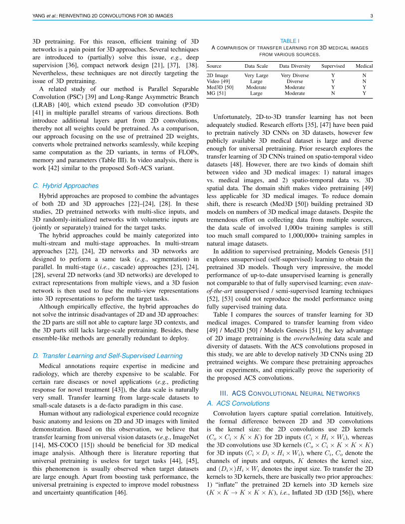
TABLE IA COMPARISON OF TRANSFER LEARNING FOR 3D MEDICAL IMAGES

FROM VARIOUS SOURCES.

Source Data Scale Data Diversity Supervised Medical

2D Image Very Large Very Diverse Y NVideo [49] Large Diverse Y NMed3D [50] Moderate Moderate Y YMG [51] Large Moderate N Y

Unfortunately, 2D-to-3D transfer learning has not beenadequately studied. Research efforts [35], [47] have been paidto pretrain natively 3D CNNs on 3D datasets, however fewpublicly available 3D medical dataset is large and diverseenough for universal pretraining. Prior research explores thetransfer learning of 3D CNNs trained on spatio-temporal videodatasets [48]. However, there are two kinds of domain shiftbetween video and 3D medical images: 1) natural imagesvs. medical images, and 2) spatio-temporal data vs. 3Dspatial data. The domain shift makes video pretraining [49]less applicable for 3D medical images. To reduce domainshift, there is research (Med3D [50]) building pretrained 3Dmodels on numbers of 3D medical image datasets. Despite thetremendous effort on collecting data from multiple sources,the data scale of involved 1,000+ training samples is stilltoo much small compared to 1,000,000+ training samples innatural image datasets.

In addition to supervised pretraining, Models Genesis [51]explores unsupervised (self-supervised) learning to obtain thepretrained 3D models. Though very impressive, the modelperformance of up-to-date unsupervised learning is generallynot comparable to that of fully supervised learning; even state-of-the-art unsupervised / semi-supervised learning techniques[52], [53] could not reproduce the model performance usingfully supervised training data.

Table I compares the sources of transfer learning for 3Dmedical images. Compared to transfer learning from video[49] / Med3D [50] / Models Genesis [51], the key advantageof 2D image pretraining is the overwhelming data scale anddiversity of datasets. With the ACS convolutions proposed inthis study, we are able to develop natively 3D CNNs using 2Dpretrained weights. We compare these pretraining approachesin our experiments, and empirically prove the superiority ofthe proposed ACS convolutions.

III. ACS CONVOLUTIONAL NEURAL NETWORKS

A. ACS ConvolutionsConvolution layers capture spatial correlation. Intuitively,

the formal difference between 2D and 3D convolutionsis the kernel size: the 2D convolutions use 2D kernels(Co × Ci ×K ×K) for 2D inputs (Ci ×Hi ×Wi), whereasthe 3D convolutions use 3D kernels (Co × Ci ×K ×K ×K)for 3D inputs (Ci×Di×Hi×Wi), where Ci, Co denote thechannels of inputs and outputs, K denotes the kernel size,and (Di×)Hi×Wi denotes the input size. To transfer the 2Dkernels to 3D kernels, there are basically two prior approaches:1) “inflate” the pretrained 2D kernels into 3D kernels size(K ×K → K ×K ×K), i.e., Inflated 3D (I3D [56]), where


ACS Convolution

Neural Networks

2D Convolution

Neural Networks

𝐶𝑖 × 𝐶𝑜(𝑎)

× 𝐾 × 𝐾 × 1

𝐶𝑖 × 𝐶𝑜(𝑐)

× 𝐾 × 1 × 𝐾

𝐶𝑖 × 𝐶𝑜(𝑠)

× 1 × 𝐾 × 𝐾 𝐶𝑜

(𝑠)× 𝐷𝑜 × 𝐻𝑜 × 𝑊𝑜

𝐶𝑜(𝑎)

× 𝐷𝑜 × 𝐻𝑜 × 𝑊𝑜

𝐶𝑜(𝑐)

× 𝐷𝑜 × 𝐻𝑜 × 𝐻𝑜

𝑐𝑜𝑛𝑐𝑎𝑡𝑒𝑛𝑎𝑡𝑒

𝐶𝑜 × 𝐷𝑜 × 𝐻𝑜 × 𝑊𝑜

𝐶𝑖 × 𝐶𝑜 × 𝐾 × 𝐾

𝐶𝑖 × 𝐻𝑖 × 𝑊𝑖

2D Convolutions to

ACS Convolutions

2D Convolutions ACS Convolutions

𝐶𝑜 × 𝐻𝑜 × 𝑊𝑜 𝐶𝑖 × 𝐷𝑖 × 𝐻𝑖 × 𝑊𝑖

2D Images 2D Representations3D Images 3D Representations

2D Inputs

2D Kernels

2D Outputs 3D Inputs

ACS Kernels

Output

3D Outputs

𝐶𝑜𝑛𝑣2𝐷




𝑊𝑎

ACS Kernels 𝑊𝑐

ACS Kernels 𝑊𝑠

𝑊

𝑋𝑜(𝑐)

Output 𝑋𝑜(𝑎)

Output 𝑋𝑜(𝑠)

𝑋𝑜 𝑋𝑖

Fig. 2. Illustration of ACS convolutions and 2D-to-ACS model conversion. With a kernel-splitting design, a 2D convolution kernel could beseamlessly transferred into ACS convolution kernels to perform natively 3D representation learning. The ACS convolutions enable ANY 2D model(ResNet [54], DenseNet [55], or DeepLab [34]) to be converted into a 3D model.

the 2D kernels are repeated along an axis and then normalized;2) unsqueeze the 2D kernels into pseudo 3D kernels on an axis(K ×K → 1×K ×K), i.e., AH-Net-like [57], which couldnot effectively capture 3D contexts. Note that in both cases,the existing methods assume a specific axis to transfer the 2Dkernels. It is meaningful to assign a special axis for spatio-temporal videos, while controversial for 3D medical images.Even for anisotropic medical images, any view of a 3D imageis still a 2D spatial image.

Based on this observation, we develop ACS (axial-coronal-sagittal) convolutions to learn spatial representations from theaxial, coronal and sagittal views. Instead of treating channelsof 2D kernels identically [56], [57], we split the kernels intothree parts for extracting 3D spatial information from the axial,coronal and sagittal views. The detailed algorithm of ACSconvolutions is shown in the supplementary materials. Forsimplicity, we introduce ACS convolutions with same paddingas follows (Fig. 2).

Given a 3D input Xi ∈ RCi×Di×Hi×Wi , we would like toobtain a 3D output Xo ∈ RCo×Do×Ho×Wo , with pretrained/ non-pretrained 2D kernels W ∈ RCo×Ci×K×K . Here, Ci

and Co denote the input and output channels, Di ×Hi ×Wi

and Do × Ho × Wo denote the input and output sizes, Kdenotes the kernel size. Instead of presenting 3D images intotri-planar 2D images [16], we split and reshape the kernelsinto three parts (named ACS kernels) by the output channel,to obtain the view-based 3D representations for each volume:Wa ∈ RC(a)

o ×Ci×K×K×1, Wc ∈ RC(c)o ×Ci×K×1×K , Ws ∈

RC(s)o ×Ci×1×K×K , where C

(a)o + C

(c)o + C

(s)o = Co. It is

theoretically possible to assign an “optimal axis” for a 2Dkernel; However, considering the feature redundancy in CNNs[58], in practice we simply set C(a)

o ≈ C(c)o ≈ C(s)

o ≈ bCo/3c.We then compute the axial, coronal and sagittal view-based 3Dfeatures via 3D convolutions:

X(a)o = Conv3D(Xi,Wa) ∈ RC(a)

o ×Do×Ho×Wo , (1)

X(c)o = Conv3D(Xi,Wc) ∈ RC(c)

o ×Do×Ho×Wo , (2)

TABLE IIMAIN OPERATOR CONVERSION FROM 2D CNNS INTO ACS CNNS.({1,K})×K ×K AND (1×)1× 1 DENOTE THE KERNEL SIZES.

2D CNNs ACS CNNs

Conv2D K ×K ACSConv K ×KConv2D 1× 1 Conv3D 1× 1× 1

{Batch,Group}Norm2D {Batch,Group}Norm3D{Max,Avg}Pool2D K ×K {Max,Avg}Pool3D {1,K} ×K ×K

X(s)o = Conv3D(Xi,Ws) ∈ RC(s)

o ×Do×Ho×Wo . (3)

The output feature Xo is obtained by concatenating X(a)o ,

X(c)o and X(s)

o by the channel axis. It is noteworthy that, no3D fusion layer is required additionally. The view-basedoutput features will be automatically fused by subsequentconvolution layers, without any additional operation, since theconvolution kernels are not split by input channel. Thanksto linearity of convolutions, expectation of features fromconverted ACS convolutions keeps the same as that of 2Dones, thereby no weight rescaling [56] is needed. It is alsothe prerequisite for the usefulness of 2D pretraining in theconverted ACS convolutions. The ACS convolution could beregarded as a special case of 3D convolutions, whose kernelsare block sparse.

The parameter size of ACS convolutions is exactly same asthat of 2D convolutions, as the ACS kernels: Wa, Wc andWs are directly split and reshaped from the 2D kernels W ,therefore the proposed method enables ANY 2D model to beconverted into a 3D model. Table II lists how operators in 2DCNNs are converted to those in ACS CNNs. Note that theconverted models could load the 2D weights directly.

B. Counterparts and Related Methods1) 2D Convolutions: We include a simple AH-Net-like [57]

2D counterpart, by replacing all ACS convolutions in ACSCNNs with Conv3D 1 × K × K. We name this pseudo 3Dcounterpart as “2.5D” in our experiments, which enables 2D


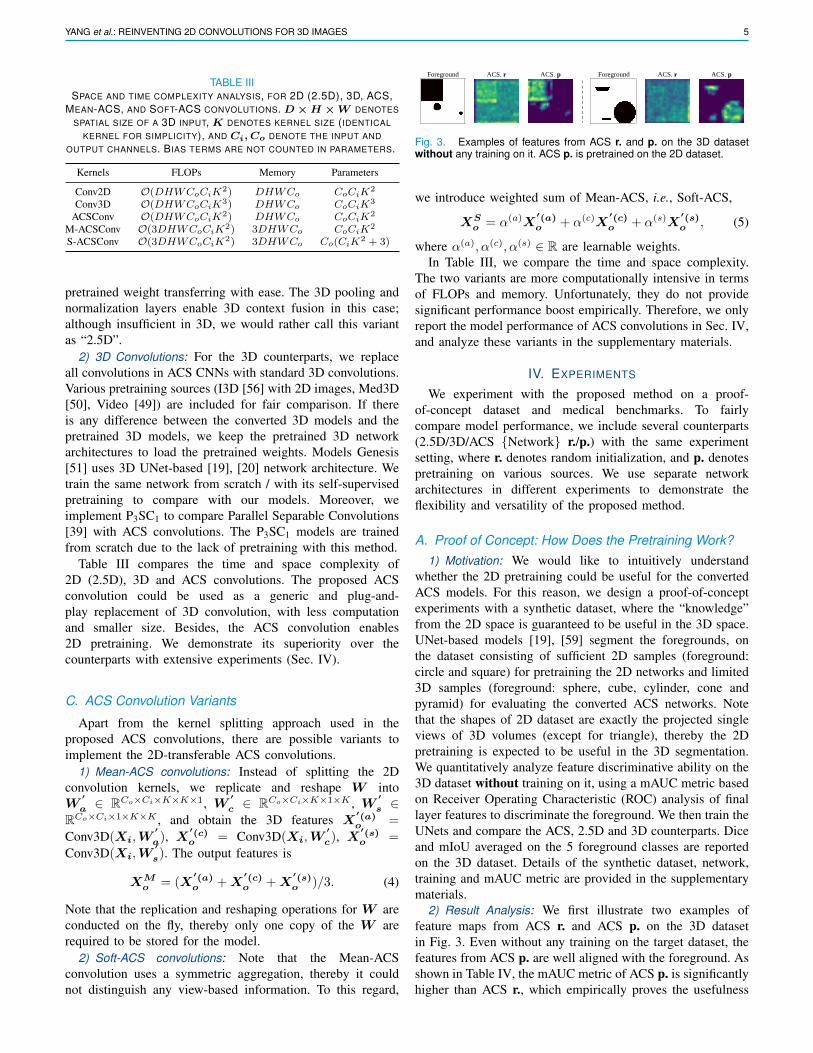
TABLE IIISPACE AND TIME COMPLEXITY ANALYSIS, FOR 2D (2.5D), 3D, ACS,

MEAN-ACS, AND SOFT-ACS CONVOLUTIONS. D ×H ×W DENOTES

SPATIAL SIZE OF A 3D INPUT, K DENOTES KERNEL SIZE (IDENTICAL

KERNEL FOR SIMPLICITY), AND Ci, Co DENOTE THE INPUT AND

OUTPUT CHANNELS. BIAS TERMS ARE NOT COUNTED IN PARAMETERS.

Kernels FLOPs Memory Parameters

Conv2D O(DHWCoCiK2) DHWCo CoCiK

2

Conv3D O(DHWCoCiK3) DHWCo CoCiK

3

ACSConv O(DHWCoCiK2) DHWCo CoCiK

2

M-ACSConv O(3DHWCoCiK2) 3DHWCo CoCiK

2

S-ACSConv O(3DHWCoCiK2) 3DHWCo Co(CiK

2 + 3)

pretrained weight transferring with ease. The 3D pooling andnormalization layers enable 3D context fusion in this case;although insufficient in 3D, we would rather call this variantas “2.5D”.

2) 3D Convolutions: For the 3D counterparts, we replaceall convolutions in ACS CNNs with standard 3D convolutions.Various pretraining sources (I3D [56] with 2D images, Med3D[50], Video [49]) are included for fair comparison. If thereis any difference between the converted 3D models and thepretrained 3D models, we keep the pretrained 3D networkarchitectures to load the pretrained weights. Models Genesis[51] uses 3D UNet-based [19], [20] network architecture. Wetrain the same network from scratch / with its self-supervisedpretraining to compare with our models. Moreover, weimplement P3SC1 to compare Parallel Separable Convolutions[39] with ACS convolutions. The P3SC1 models are trainedfrom scratch due to the lack of pretraining with this method.

Table III compares the time and space complexity of2D (2.5D), 3D and ACS convolutions. The proposed ACSconvolution could be used as a generic and plug-and-play replacement of 3D convolution, with less computationand smaller size. Besides, the ACS convolution enables2D pretraining. We demonstrate its superiority over thecounterparts with extensive experiments (Sec. IV).

C. ACS Convolution Variants

Apart from the kernel splitting approach used in theproposed ACS convolutions, there are possible variants toimplement the 2D-transferable ACS convolutions.

1) Mean-ACS convolutions: Instead of splitting the 2Dconvolution kernels, we replicate and reshape W intoW

′

a ∈ RCo×Ci×K×K×1, W′

c ∈ RCo×Ci×K×1×K , W′

s ∈RCo×Ci×1×K×K , and obtain the 3D features X

′(a)o =

Conv3D(Xi,W′

a), X′(c)o = Conv3D(Xi,W

′

c), X′(s)o =

Conv3D(Xi,W′

s). The output features is

XMo = (X

′(a)o +X

′(c)o +X

′(s)o )/3. (4)

Note that the replication and reshaping operations for W areconducted on the fly, thereby only one copy of the W arerequired to be stored for the model.

2) Soft-ACS convolutions: Note that the Mean-ACSconvolution uses a symmetric aggregation, thereby it couldnot distinguish any view-based information. To this regard,

Foreground ACS. r ACS. p ACS. r ACS. Foreground p

Fig. 3. Examples of features from ACS r. and p. on the 3D datasetwithout any training on it. ACS p. is pretrained on the 2D dataset.

we introduce weighted sum of Mean-ACS, i.e., Soft-ACS,

XSo = α(a)X

′(a)o + α(c)X

′(c)o + α(s)X

′(s)o , (5)

where α(a), α(c), α(s) ∈ R are learnable weights.In Table III, we compare the time and space complexity.

The two variants are more computationally intensive in termsof FLOPs and memory. Unfortunately, they do not providesignificant performance boost empirically. Therefore, we onlyreport the model performance of ACS convolutions in Sec. IV,and analyze these variants in the supplementary materials.

IV. EXPERIMENTS

We experiment with the proposed method on a proof-of-concept dataset and medical benchmarks. To fairlycompare model performance, we include several counterparts(2.5D/3D/ACS {Network} r./p.) with the same experimentsetting, where r. denotes random initialization, and p. denotespretraining on various sources. We use separate networkarchitectures in different experiments to demonstrate theflexibility and versatility of the proposed method.

A. Proof of Concept: How Does the Pretraining Work?1) Motivation: We would like to intuitively understand

whether the 2D pretraining could be useful for the convertedACS models. For this reason, we design a proof-of-conceptexperiments with a synthetic dataset, where the “knowledge”from the 2D space is guaranteed to be useful in the 3D space.UNet-based models [19], [59] segment the foregrounds, onthe dataset consisting of sufficient 2D samples (foreground:circle and square) for pretraining the 2D networks and limited3D samples (foreground: sphere, cube, cylinder, cone andpyramid) for evaluating the converted ACS networks. Notethat the shapes of 2D dataset are exactly the projected singleviews of 3D volumes (except for triangle), thereby the 2Dpretraining is expected to be useful in the 3D segmentation.We quantitatively analyze feature discriminative ability on the3D dataset without training on it, using a mAUC metric basedon Receiver Operating Characteristic (ROC) analysis of finallayer features to discriminate the foreground. We then train theUNets and compare the ACS, 2.5D and 3D counterparts. Diceand mIoU averaged on the 5 foreground classes are reportedon the 3D dataset. Details of the synthetic dataset, network,training and mAUC metric are provided in the supplementarymaterials.

2) Result Analysis: We first illustrate two examples offeature maps from ACS r. and ACS p. on the 3D datasetin Fig. 3. Even without any training on the target dataset, thefeatures from ACS p. are well aligned with the foreground. Asshown in Table IV, the mAUC metric of ACS p. is significantlyhigher than ACS r., which empirically proves the usefulness


TABLE IVSEGMENTATION PERFORMANCE ON THE PROOF-OF-CONCEPT DATASET.

Models Feature mAUC w/o training Dice mIoU Size

2.5D UNet r. 69.0 82.2 72.5 1.6 Mb2.5D UNet p. 85.1 82.7 73.3 1.6 Mb3D UNet r. 72.1 94.6 90.8 4.7 Mb

ACS UNet r. 68.7 94.7 90.7 1.6 MbACS UNet p. 88.1 95.4 92.0 1.6 Mb

TABLE VLIDC-IDRI [60] LUNG NODULE SEGMENTATION (DICE GLOBAL) AND

CLASSIFICATION (AUC) PERFORMANCE.

Models Segmentation (Dice) Classification (AUC)

Models Genesis [51] r. 75.5 94.3Models Genesis [51] p. 75.9 94.1P3SC1 [39] r. 74.3 90.9

2.5D ResNet-18 r. 68.8 89.42.5D ResNet-18 p. 69.8 92.03D ResNet-18 r. 74.7 90.33D ResNet-18 p. I3D [56] 75.7 91.53D ResNet-18 p. Med3D [50] 74.9 90.63D ResNet-18 p. Video [49] 75.7 91.0

ACS ResNet-18 r. 75.1 92.5ACS ResNet-18 p. 76.5 94.9

of pretraining for ACS convolutions. Notably, features fromACS p. are even more discriminative than 2.5D p. Aftertraining on the 3D dataset, the performance of ACS UNet r. iscomparable to 3D UNet r., and the ACS UNet p. achieves thebest performance. The results indicate that ACS convolutionis an alternative to 3D convolution with comparable or evenbetter performance, and a smaller model size.

B. Lung Nodule Classification and Segmentation

1) Dataset: We then validate the effectiveness of theproposed method on a large medical data LIDC-IDRI [60],the largest public lung nodule dataset, for both lung nodulesegmentation and malignancy classification task. There are2, 635 lung nodules annotated by at most 4 experts, from1, 018 CT scans. The annotations include pixel-level labellingof the nodules and 5-level classification of the malignancy,from “1” (highly benign) to “5” (highly malignant). Forsegmentation, we choose one of the up to 4 annotationsfor all cases. For classification, we take the mode of theannotations as its category. In order to reduce ambiguity,we ignore nodules with level-“3” (uncertain labelling) andperform binary classification by categorizing the cases withlevel “1/2”, “4/5” into class 0, 1. It results in a total of 1,633nodules for classification. We randomly divide the dataset into4 : 1 for training and evaluation, respectively. At trainingstage we perform data augmentation including random-centercropping, random-axis rotation and flipping.

2) Experiment Setting: We compare the ACS models with2.5D and 3D counterparts with or without pretraining. Thepretrained 2.5D / ACS weights are from PyTorch torchvisionpackage [25], trained on ImageNet [14]. For 3D pretraining,we use the official pretrained models by Med3D [50] and

Video [49], while I3D [56] weights are transformed fromthe 2D ImageNet-pretrained weights as well. For PSC [39],we use the configuration of P3SC1, which resembles ourACS methods. To take advantage of the pretrained weightsfrom Med3D [50] and video [49] for comparison, all modelsare adopted a ResNet-18 [54] architecture, except for ModelGenesis [51], since the official pretrained model is based on a3D UNet [19] architecture. For all model training, we use anAdam optimizer [61] with an initial learning rate of 0.001 andtrain the model for 100 epochs, and delay the learning rate by0.1 after 50 and 75 epochs. For ResNet-18 backbone, in orderto keep higher resolution for output feature maps, we modifythe stride of first layer (7 × 7 stride-2 convolution) into 1,and remove the first max-pooling. Note that this modificationstill enables pretraining. A FCN-like [31] decoder is appliedwith progressive upsampling twice. Dice loss with a batchof 8 is used for segmentation, and binary cross-entropy losswith a batch of 24 for classification. Dice global and AUC arereported for these two tasks. To demonstrate the flexibility andversatility of ACS convolutions, we also report the results ofVGG [62] and DenseNet [55] in the supplementary materials,which is consistent with the ResNet-18.

To further demonstrate the effectiveness of pretraining,we evaluate models trained with various percentages oftraining data (25%, 50%, 75% and 100%) on bothsegmentation and classification. To maintain the same numberof training iterations, the numbers of epoch are increased to100/(0.25, 0.5, 0.75, 1). The best results among all epochs arereported. We plot the results in Fig. 4.

3) Result Analysis: Experiment results are depicted inTable V. The ACS models consistently outperform all thecounterparts by large margins, including 2.5D and 3D modelsin both random initialization or pretraining settings. P3SC1[39] performance is similar to standard 3D convolution.We observe that the 3D models (ACS, PSC and 3D)generally outperform the 2.5D models, indicating that theusefulness of 3D contexts. Except for the pretrained 2.5Dmodel on classification task, its superior performance over3D counterparts may explain the prior art [63], [64] with 2Dnetworks on this dataset. As for pretraining, the ImageNet[14] provides significant performance boost (see 2.5D p.,3D p. I3D [56] and ACS p.), while Med3D [50] bringslimited performance boost. We conjecture that it owes to theoverwhelming data scale and diversity of 2D image dataset.

Due to the difference on network architecture (ResNet-based FCN vs. UNet), we experiment with the official code ofself-supervised pretrained Models Genesis [51] with exactlysame setting. Even without pretraining, the segmentationand classification performance of the UNet-based modelsare strong on this dataset. Despite this, the pretrained ACSmodel is still better performing. Besides, negative transferringis observed for classification experiments by the ModelsGenesis [51] encoder-only transferring, whereas the ImageNetpretraining consistently improves the performance. Apart fromthe superior model performance, the ACS model achievesthe best parameter efficiency in our experiments. Take thesegmentation task for example, the size of ACS model is 49.8Mb, compared to 49.8 Mb (2.5D), 142.5 Mb (3D) and 65.4


82

84

86

88

90

92

94

96

0.25 0.5 0.75 1

ACS p. ACS r.82

84

86

88

90

92

94

96

0.25 0.5 0.75 1

3D r. I3D

Med3D Video82

84

86

88

90

92

94

96

0.25 0.5 0.75 1

2.5D p. 2.5D r.82

84

86

88

90

92

94

96

0.25 0.5 0.75 1

Models Genesis p.

Models Genesis r.

ACS (ResNet-18) 2.5D (ResNet-18) 3D (ResNet-18) Models Genesis (UNet)

Clas

sific

atio

n (A

UC)

73

74

75

76

77

0.25 0.5 0.75 1

ACS p. ACS r.73

74

75

76

77

0.25 0.5 0.75 1

3D r. I3D Med3D Video

67

69

71

73

75

77

0.25 0.5 0.75 1

2.5D p. 2.5D r.

73

74

75

76

77

0.25 0.5 0.75 1

Models Genesis p.

Models Genesis r.

Segm

enta

tion

(Dic

e)

Fig. 4. Performance of ACS, 2.5D, 3D and MG [51] on LIDC-IDRI [60] lung nodule classification and segmentation vs. the training data scale.

TABLE VILITS [65] SEGMENTATION PERFORMANCE ON LESION AND LIVER. DG:

DICE GLOBAL. DPC: DICE PER CASE.

Models Lesion LiverDG DPC DG DPC

H-DenseUNet [22] 82.4 72.2 96.5 96.1Models Genesis [51]2 - - - 91.13 ±1.51P3SC1 [39] r. 72.6 59.1 93.9 94.2

2.5D DeepLab r. 72.9 56.9 93.1 92.72.5D DeepLab p. 73.4 60.4 92.9 92.03D DeepLab r. 75.5 62.6 94.8 94.83D DeepLab p. I3D [56] 76.5 58.2 94.1 93.43D DeepLab p. Med3D [50] 67.1 53.9 92.0 93.63D DeepLab p. Video [49] 66.3 56.9 92.5 93.2

ACS DeepLab r. 75.3 62.4 95.0 94.9ACS DeepLab p. 79.1 65.8 96.7 96.2

Mb (MG [51]).As showed in Fig 4, models with pretraining consistently

outperform those without pretraining under various trainingdata scales. Moreover, when trained with 25% data, theperformance gap between p. and n. reaches the highest, whichimplies the efficiency of pretraining for limited annotated data.Note that ACS p. consistently outperforms all counterparts, nomatter how much training data are leveraged.

C. Liver Tumor Segmentation (LiTS) Benchmark

1) Dataset: We further experiment with our approach onLiTS [65], a challenging 3D medical image segmentationdataest. It consists of 131 and 70 enhanced abdominal CTscans for training and testing respectively, to segment the liverand liver tumors. The training annotations are open to publicwhile the test ones are only accessible by online evaluation.The sizes of x, y axis are 512, while the sizes of z axis varyin the range of [50, 1000]. We transpose the axes into z, y, xto keep the concept consistent as previously mentioned. Forpre-processing, we clip the Hounsfield Unit to [−200, 250] andthen normalize to [0, 1]. Training data augmentation includesrandom-center cropping, random-axis flipping and rotation,and random-scale resampling.

2The author only releases the pretrained model on chest CTs, thereby wesimply report the evaluation metric provided by the paper.

2) Experiment Setting: A DeepLabv3+ [34] with abackbone of ResNet-101 [54] is used in this experiment.The pretrained 2D model is directly obtained from PyTorchtorchvision package [25]. The compared baselines are similarto those in the above LIDC experiment (Sec. IV-B). We trainall the models for 6000 epochs. An Adam optimizer [61] isused with an initial learning rate of 0.001, and we decay thelearning rate by 0.1 after 3000 and 4500 epochs. At trainingstage, we crop the volumes to the size of 64×224×224. As fortesting stage, we crop the volumes to the size of 64×512×512and adopt window sliding at a step of 24 at z axis. Dice globaland Dice per case of lesion and liver are reported as standardevaluation on this dataset.

3) Result Analysis: As shown in Table VI, consistent modelperformance as LIDC experiment (Sec. IV-B) can be observed.The pretrained ACS DeepLab achieves better performancethan the 2D and 3D counterparts (including self-supervisedpretraining [51]) by large margins; without pretraining, ACSDeepLab achieves comparable or better performance than3D DeepLab. According to pretraining results on I3D [56],Med3D [50] and Video [49] for 3D DeepLab, negativetransferring is observed, probably due to severe domain shiftand anisotropy on LiTS dataset. We also report a state-of-the-art performance on LiTS dataset using H-DenseUNet [22] asa reference. Note that it adopts a completely different trainingstrategy and network architecture (a cascade of 2D and 3DDenseNet [55] models), thereby it is insuitable to compare toour models directly. It is feasible to integrate these orthogonalcontributions into ours to improve the model performance.

A key advantage of the proposed ACS convolution isthat it enables flexible whole-network conversion togetherwith the pretrained weights, including the task head. Inthe supplementary materials, we validate the superiority ofwhole-network weight transferring over encoder-only weighttransferring. The previous pretraining methods, e.g., I3D [56],Med3D [50] and Video [49], hardly take care of the scenarios.

D. Universal Lesion Detection on DeepLesion

1) Dataset: DeepLesion dataset [3] consists of 32,120 axialCT slices from 10,594 studies of unique patients. There are 1to 3 lesions in each slice, with totally 32,735 lesions fromseveral organs, whose sizes vary from 0.21 to 342.5mm.RECIST diameter coordinates and bounding boxes were


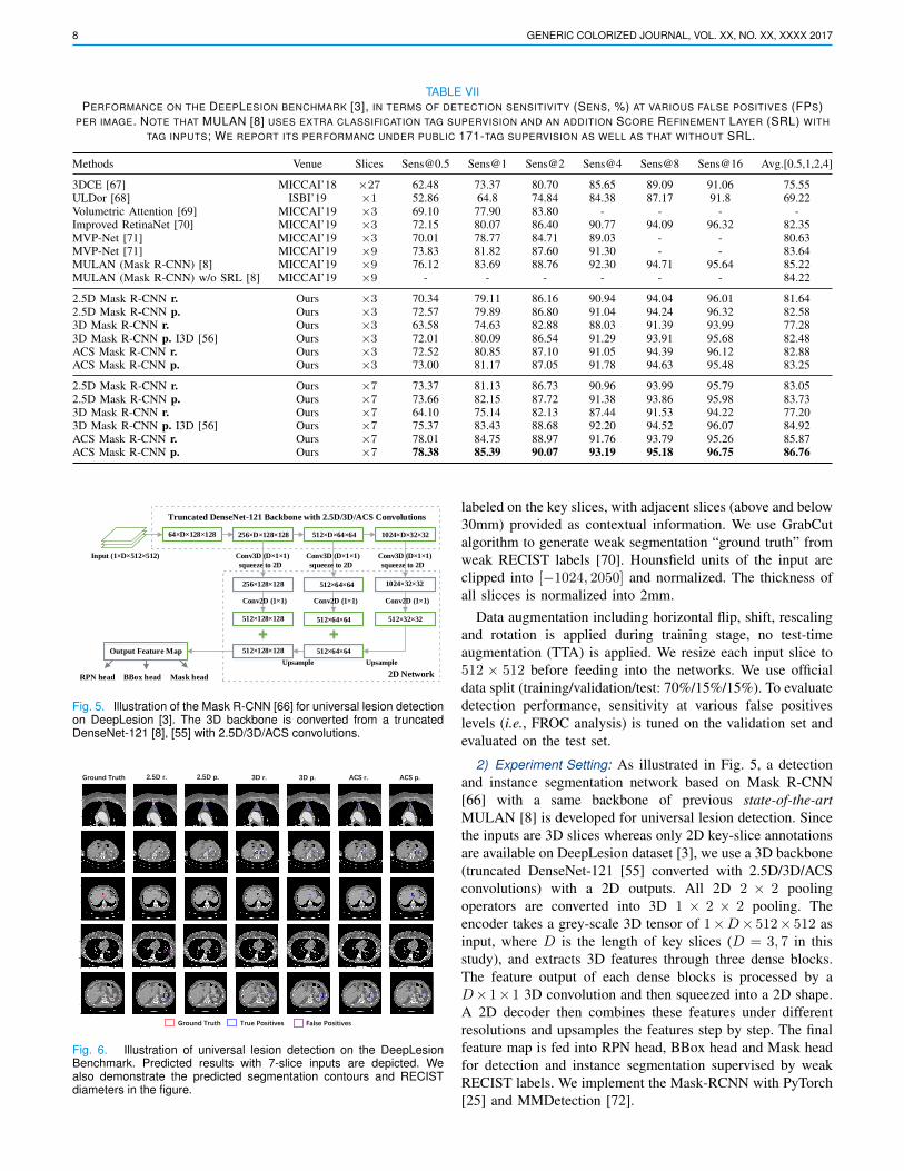
TABLE VIIPERFORMANCE ON THE DEEPLESION BENCHMARK [3], IN TERMS OF DETECTION SENSITIVITY (SENS, %) AT VARIOUS FALSE POSITIVES (FPS)

PER IMAGE. NOTE THAT MULAN [8] USES EXTRA CLASSIFICATION TAG SUPERVISION AND AN ADDITION SCORE REFINEMENT LAYER (SRL) WITH

TAG INPUTS; WE REPORT ITS PERFORMANC UNDER PUBLIC 171-TAG SUPERVISION AS WELL AS THAT WITHOUT SRL.

Methods Venue Slices [email protected] Sens@1 Sens@2 Sens@4 Sens@8 Sens@16 Avg.[0.5,1,2,4]

3DCE [67] MICCAI’18 ×27 62.48 73.37 80.70 85.65 89.09 91.06 75.55ULDor [68] ISBI’19 ×1 52.86 64.8 74.84 84.38 87.17 91.8 69.22Volumetric Attention [69] MICCAI’19 ×3 69.10 77.90 83.80 - - - -Improved RetinaNet [70] MICCAI’19 ×3 72.15 80.07 86.40 90.77 94.09 96.32 82.35MVP-Net [71] MICCAI’19 ×3 70.01 78.77 84.71 89.03 - - 80.63MVP-Net [71] MICCAI’19 ×9 73.83 81.82 87.60 91.30 - - 83.64MULAN (Mask R-CNN) [8] MICCAI’19 ×9 76.12 83.69 88.76 92.30 94.71 95.64 85.22MULAN (Mask R-CNN) w/o SRL [8] MICCAI’19 ×9 - - - - - - 84.22

2.5D Mask R-CNN r. Ours ×3 70.34 79.11 86.16 90.94 94.04 96.01 81.642.5D Mask R-CNN p. Ours ×3 72.57 79.89 86.80 91.04 94.24 96.32 82.583D Mask R-CNN r. Ours ×3 63.58 74.63 82.88 88.03 91.39 93.99 77.283D Mask R-CNN p. I3D [56] Ours ×3 72.01 80.09 86.54 91.29 93.91 95.68 82.48ACS Mask R-CNN r. Ours ×3 72.52 80.85 87.10 91.05 94.39 96.12 82.88ACS Mask R-CNN p. Ours ×3 73.00 81.17 87.05 91.78 94.63 95.48 83.25

2.5D Mask R-CNN r. Ours ×7 73.37 81.13 86.73 90.96 93.99 95.79 83.052.5D Mask R-CNN p. Ours ×7 73.66 82.15 87.72 91.38 93.86 95.98 83.733D Mask R-CNN r. Ours ×7 64.10 75.14 82.13 87.44 91.53 94.22 77.203D Mask R-CNN p. I3D [56] Ours ×7 75.37 83.43 88.68 92.20 94.52 96.07 84.92ACS Mask R-CNN r. Ours ×7 78.01 84.75 88.97 91.76 93.79 95.26 85.87ACS Mask R-CNN p. Ours ×7 78.38 85.39 90.07 93.19 95.18 96.75 86.76

Truncated DenseNet-121 Backbone with 2.5D/3D/ACS Convolutions

Input (1×D×512×512)

1024×D×32×3264×D×128×128 256×D×128×128 512×D×64×64

256×128×128

Upsample Upsample

512×128×128 512×64×64 512×32×32

512×64×64512×128×128

2D Network

512×64×64 1024×32×32

Output Feature Map

RPN head BBox head Mask head

Conv3D (D×1×1)

Conv2D (1×1) Conv2D (1×1) Conv2D (1×1)

Conv3D (D×1×1) Conv3D (D×1×1)

squeeze to 2D squeeze to 2D squeeze to 2D

Fig. 5. Illustration of the Mask R-CNN [66] for universal lesion detectionon DeepLesion [3]. The 3D backbone is converted from a truncatedDenseNet-121 [8], [55] with 2.5D/3D/ACS convolutions.

Ground Truth 2.5D r. 2.5D p. 3D r. 3D p. ACS r. ACS p.

Ground Truth True Positives False Positives

Fig. 6. Illustration of universal lesion detection on the DeepLesionBenchmark. Predicted results with 7-slice inputs are depicted. Wealso demonstrate the predicted segmentation contours and RECISTdiameters in the figure.

labeled on the key slices, with adjacent slices (above and below30mm) provided as contextual information. We use GrabCutalgorithm to generate weak segmentation “ground truth” fromweak RECIST labels [70]. Hounsfield units of the input areclipped into [−1024, 2050] and normalized. The thickness ofall slicces is normalized into 2mm.

Data augmentation including horizontal flip, shift, rescalingand rotation is applied during training stage, no test-timeaugmentation (TTA) is applied. We resize each input slice to512 × 512 before feeding into the networks. We use officialdata split (training/validation/test: 70%/15%/15%). To evaluatedetection performance, sensitivity at various false positiveslevels (i.e., FROC analysis) is tuned on the validation set andevaluated on the test set.

2) Experiment Setting: As illustrated in Fig. 5, a detectionand instance segmentation network based on Mask R-CNN[66] with a same backbone of previous state-of-the-artMULAN [8] is developed for universal lesion detection. Sincethe inputs are 3D slices whereas only 2D key-slice annotationsare available on DeepLesion dataset [3], we use a 3D backbone(truncated DenseNet-121 [55] converted with 2.5D/3D/ACSconvolutions) with a 2D outputs. All 2D 2 × 2 poolingoperators are converted into 3D 1 × 2 × 2 pooling. Theencoder takes a grey-scale 3D tensor of 1×D× 512× 512 asinput, where D is the length of key slices (D = 3, 7 in thisstudy), and extracts 3D features through three dense blocks.The feature output of each dense blocks is processed by aD×1×1 3D convolution and then squeezed into a 2D shape.A 2D decoder then combines these features under differentresolutions and upsamples the features step by step. The finalfeature map is fed into RPN head, BBox head and Mask headfor detection and instance segmentation supervised by weakRECIST labels. We implement the Mask-RCNN with PyTorch[25] and MMDetection [72].


We adopt cross entropy loss for classification and smoothL1 loss for bounding box regression in the RPN head andBBox head, while in the Mask head we adopt the dice loss.These losses weigh equally to form the final loss function. Weuse an momentum SGD optimizer to train the models for 20epochs. The learning rate is initialized as 0.02 and multipliedby 0.1 at epoch 10 and 13.

3) Result Analysis: As depicted in Table VII, the proposedACS Mask R-CNN with pretraining significantly outperformsprevious state-of-the-art MULAN [8]. Notably, we use onlythe detection and RECIST supervision, without additionalinformation beyond the CT images such as tags from medicalreports and demographic information. 3D context modelingwith 3D and ACS convolutions is proven effective, especiallywith more input slices. Pretraining consistently improves themodel performance for 2.5D, 3D and ACS convolutions. Largeperformance gap is observed for 3D r. and 3D p., perhaps dueto the large model size of 3D convolutions. We also visualizeseveral examples of detection results in Fig. 6. Both 3D contextmodeling and pretraining reduce the predicted false positives.

V. CONCLUSION

We propose ACS convolution for 3D medical images, asa generic and plug-and-play replacement of standard 3Dconvolution. It enables pretraining from 2D images, whichconsistently provides singificant performance boost in ourexperiments. Even without pretraining, the ACS convolution iscomparable or even better than 3D convolution, with smallermodel size and less computation. In further study, we willfocus on optimal ACS kernel axis assignment and integrationwith other 2D-to-3D transfer learning operators.

REFERENCES

[1] G. Litjens, T. Kooi, B. E. Bejnordi, A. A. A. Setio, F. Ciompi,M. Ghafoorian, J. A. Van Der Laak, B. Van Ginneken, and C. I. Sanchez,“A survey on deep learning in medical image analysis,” Medical imageanalysis, vol. 42, pp. 60–88, 2017.

[2] R. Droste, Y. Cai, H. Sharma, P. Chatelain, L. Drukker, A. T.Papageorghiou, and J. A. Noble, “Ultrasound image representationlearning by modeling sonographer visual attention,” in InternationalConference on Information Processing in Medical Imaging. Springer,2019, pp. 592–604.

[3] K. Yan, X. Wang, L. Lu, L. Zhang, A. P. Harrison, M. Bagheri, andR. M. Summers, “Deep lesion graphs in the wild: relationship learningand organization of significant radiology image findings in a diverselarge-scale lesion database,” in CVPR, 2018, pp. 9261–9270.

[4] B. H. Menze, A. Jakab, S. Bauer, J. Kalpathy-Cramer, K. Farahani,J. Kirby, Y. Burren, N. Porz, J. Slotboom, R. Wiest et al., “Themultimodal brain tumor image segmentation benchmark (brats),” IEEEtransactions on medical imaging, vol. 34, no. 10, pp. 1993–2024, 2014.

[5] X. Wang, Y. Peng, L. Lu, Z. Lu, M. Bagheri, and R. M. Summers,“Chestx-ray8: Hospital-scale chest x-ray database and benchmarks onweakly-supervised classification and localization of common thoraxdiseases,” in CVPR, 2017, pp. 2097–2106.

[6] V. Gulshan, L. Peng, M. Coram, M. C. Stumpe, D. Wu,A. Narayanaswamy, S. Venugopalan, K. Widner, T. Madams, J. Cuadroset al., “Development and validation of a deep learning algorithm fordetection of diabetic retinopathy in retinal fundus photographs,” Jama,vol. 316, no. 22, pp. 2402–2410, 2016.

[7] F. Isensee, J. Petersen, A. Klein, D. Zimmerer, P. F. Jaeger, S. Kohl,J. Wasserthal, G. Koehler, T. Norajitra, S. Wirkert et al., “nnu-net: Self-adapting framework for u-net-based medical image segmentation,” arXivpreprint arXiv:1809.10486, 2018.

[8] K. Yan, Y. Tang, Y. Peng, V. Sandfort, M. Bagheri, Z. Lu, and R. M.Summers, “Mulan: Multitask universal lesion analysis network for jointlesion detection, tagging, and segmentation,” in MICCAI. Springer,2019, pp. 194–202.

[9] G. Balakrishnan, A. Zhao, M. R. Sabuncu, J. Guttag, and A. V. Dalca,“Voxelmorph: a learning framework for deformable medical imageregistration,” IEEE transactions on medical imaging, 2019.

[10] A. A. A. Setio, A. Traverso, T. De Bel, M. S. Berens, C. van denBogaard, P. Cerello, H. Chen, Q. Dou, M. E. Fantacci, B. Geurts et al.,“Validation, comparison, and combination of algorithms for automaticdetection of pulmonary nodules in computed tomography images: theluna16 challenge,” Medical image analysis, vol. 42, pp. 1–13, 2017.

[11] A. L. Simpson, M. Antonelli, S. Bakas, M. Bilello, K. Farahani,B. van Ginneken, A. Kopp-Schneider, B. A. Landman, G. Litjens,B. Menze et al., “A large annotated medical image dataset for thedevelopment and evaluation of segmentation algorithms,” arXiv preprintarXiv:1902.09063, 2019.

[12] N. Tajbakhsh, L. Jeyaseelan, Q. Li, J. Chiang, Z. Wu, and X. Ding,“Embracing imperfect datasets: A review of deep learning solutionsfor medical image segmentation.” Medical image analysis, vol. 63, p.101693, 2020.

[13] K. Yan, Y. Peng, V. Sandfort, M. Bagheri, Z. Lu, and R. M. Summers,“Holistic and comprehensive annotation of clinically significant findingson diverse ct images: Learning from radiology reports and labelontology,” in CVPR, 2019, pp. 8523–8532.

[14] J. Deng, W. Dong, R. Socher, L.-J. Li, K. Li, and L. Fei-Fei, “Imagenet:A large-scale hierarchical image database,” in CVPR. Ieee, 2009, pp.248–255.

[15] T.-Y. Lin, M. Maire, S. Belongie, J. Hays, P. Perona, D. Ramanan,P. Dollar, and C. L. Zitnick, “Microsoft coco: Common objects incontext,” in ECCV. Springer, 2014, pp. 740–755.

[16] H. R. Roth, L. Lu, A. Seff, K. M. Cherry, J. Hoffman, S. Wang, J. Liu,E. Turkbey, and R. M. Summers, “A new 2.5 d representation for lymphnode detection using random sets of deep convolutional neural networkobservations,” in MICCAI. Springer, 2014, pp. 520–527.

[17] Q. Yu, L. Xie, Y. Wang, Y. Zhou, E. K. Fishman, and A. L. Yuille,“Recurrent saliency transformation network: Incorporating multi-stagevisual cues for small organ segmentation,” in CVPR, 2018, pp. 8280–8289.

[18] T. Ni, L. Xie, H. Zheng, E. K. Fishman, and A. L. Yuille, “Elasticboundary projection for 3d medical image segmentation,” in CVPR,2019, pp. 2109–2118.

[19] O. Cicek, A. Abdulkadir, S. S. Lienkamp, T. Brox, and O. Ronneberger,“3d u-net: learning dense volumetric segmentation from sparseannotation,” in MICCAI. Springer, 2016, pp. 424–432.

[20] F. Milletari, N. Navab, and S.-A. Ahmadi, “V-net: Fully convolutionalneural networks for volumetric medical image segmentation,” in 3DV.IEEE, 2016, pp. 565–571.

[21] W. Zhao, J. Yang, Y. Sun, C. Li, W. Wu, L. Jin, Z. Yang, B. Ni,P. Gao, P. Wang et al., “3d deep learning from ct scans predicts tumorinvasiveness of subcentimeter pulmonary adenocarcinomas,” Cancerresearch, vol. 78, no. 24, pp. 6881–6889, 2018.

[22] X. Li, H. Chen, X. Qi, Q. Dou, C.-W. Fu, and P.-A. Heng, “H-denseunet:hybrid densely connected unet for liver and tumor segmentation from ctvolumes,” IEEE transactions on medical imaging, vol. 37, no. 12, pp.2663–2674, 2018.

[23] Y. Xia, L. Xie, F. Liu, Z. Zhu, E. K. Fishman, and A. L. Yuille, “Bridgingthe gap between 2d and 3d organ segmentation with volumetric fusionnet,” in MICCAI. Springer, 2018, pp. 445–453.

[24] H. Zheng, Y. Zhang, L. Yang, P. Liang, Z. Zhao, C. Wang, and D. Z.Chen, “A new ensemble learning framework for 3d biomedical imagesegmentation,” in AAAI, vol. 33, 2019, pp. 5909–5916.

[25] A. Paszke, S. Gross, S. Chintala, G. Chanan, E. Yang, Z. DeVito, Z. Lin,A. Desmaison, L. Antiga, and A. Lerer, “Automatic differentiation inPyTorch,” in NIPS Autodiff Workshop, 2017.

[26] A. Prasoon, K. Petersen, C. Igel, F. Lauze, E. Dam, and M. Nielsen,“Deep feature learning for knee cartilage segmentation using a triplanarconvolutional neural network,” MICCAI, vol. 16 Pt 2, pp. 246–53, 2013.

[27] J. Ding, A. Li, Z. Hu, and L. Wang, “Accurate pulmonary noduledetection in computed tomography images using deep convolutionalneural networks,” in MICCAI, 2017.

[28] M. Perslev, E. B. Dam, A. Pai, and C. Igel, “One network to segmentthem all: A general, lightweight system for accurate 3d medical imagesegmentation,” in MICCAI. Springer, 2019, pp. 30–38.

[29] Y. Xia, F. Liu, D. Yang, J. Cai, L. Yu, Z. Zhu, D. Xu, A. Yuille, andH. Roth, “3d semi-supervised learning with uncertainty-aware multi-


view co-training,” in The IEEE Winter Conference on Applications ofComputer Vision, 2020, pp. 3646–3655.

[30] Y. Song, Z. Yu, T. Zhou, J. Y.-C. Teoh, B. Lei, K.-S. Choi, andJ. Qin, “Learning 3d features with 2d cnns via surface projection for ctvolume segmentation,” in International Conference on Medical ImageComputing and Computer-Assisted Intervention. Springer, 2020, pp.176–186.

[31] J. Long, E. Shelhamer, and T. Darrell, “Fully convolutional networksfor semantic segmentation,” CVPR, pp. 3431–3440, 2015.

[32] A. Esteva, B. Kuprel, R. A. Novoa, J. Ko, S. M. Swetter, H. M. Blau,and S. Thrun, “Dermatologist-level classification of skin cancer withdeep neural networks,” Nature, vol. 542, no. 7639, p. 115, 2017.

[33] T.-Y. Lin, P. Goyal, R. Girshick, K. He, and P. Dollar, “Focal loss fordense object detection,” in ICCV, 2017, pp. 2980–2988.

[34] L.-C. Chen, Y. Zhu, G. Papandreou, F. Schroff, and H. Adam,“Encoder-decoder with atrous separable convolution for semantic imagesegmentation,” in ECCV, 2018, pp. 801–818.

[35] K. Kamnitsas, C. Ledig, V. F. Newcombe, J. P. Simpson, A. D. Kane,D. K. Menon, D. Rueckert, and B. Glocker, “Efficient multi-scale 3dcnn with fully connected crf for accurate brain lesion segmentation,”Medical image analysis, vol. 36, pp. 61–78, 2017.

[36] Q. Dou, L. Yu, H. Chen, Y. Jin, X. Yang, J. Qin, and P.-A. Heng, “3ddeeply supervised network for automated segmentation of volumetricmedical images,” Medical image analysis, vol. 41, pp. 40–54, 2017.

[37] Z. Zhou, M. M. R. Siddiquee, N. Tajbakhsh, and J. Liang, “Unet++:A nested u-net architecture for medical image segmentation,” in DeepLearning in Medical Image Analysis and Multimodal Learning forClinical Decision Support. Springer, 2018, pp. 3–11.

[38] J. Zhang, Y. Xie, P. Zhang, H. Chen, Y. Xia, and C. Shen, “Light-weighthybrid convolutional network for liver tumor segmentation.” in IJCAI,2019, pp. 4271–4277.

[39] F. Gonda, D. Wei, T. Parag, and H. Pfister, “Parallel separable 3dconvolution for video and volumetric data understanding,” in BMVC,2018.

[40] H. Zheng, L. Yang, J. Han, Y. Zhang, P. Liang, Z. Zhao, C. Wang,and D. Z. Chen, “Hfa-net: 3d cardiovascular image segmentationwith asymmetrical pooling and content-aware fusion,” in InternationalConference on Medical Image Computing and Computer-AssistedIntervention. Springer, 2019, pp. 759–767.

[41] Z. Qiu, T. Yao, and T. Mei, “Learning spatio-temporal representationwith pseudo-3d residual networks,” ICCV, pp. 5534–5542, 2017.

[42] C. Li, Q. Zhong, D. Xie, and S. Pu, “Collaborative spatiotemporalfeature learning for video action recognition,” in Proceedings of theIEEE Conference on Computer Vision and Pattern Recognition, 2019,pp. 7872–7881.

[43] R. Sun, E. J. Limkin, M. Vakalopoulou, L. Dercle, S. Champiat, S. R.Han, L. Verlingue, D. Brandao, A. Lancia, S. Ammari et al., “Aradiomics approach to assess tumour-infiltrating cd8 cells and responseto anti-pd-1 or anti-pd-l1 immunotherapy: an imaging biomarker,retrospective multicohort study,” The Lancet Oncology, vol. 19, no. 9,pp. 1180–1191, 2018.

[44] K. He, R. Girshick, and P. Dollar, “Rethinking imagenet pre-training,”in CVPR, 2019, pp. 4918–4927.

[45] M. Raghu, C. Zhang, J. Kleinberg, and S. Bengio, “Transfusion:Understanding transfer learning with applications to medical imaging,”in NeurIPS, 2019.

[46] D. Hendrycks, K. Lee, and M. Mazeika, “Using pre-training canimprove model robustness and uncertainty,” in ICML, ser. Proceedingsof Machine Learning Research, K. Chaudhuri and R. Salakhutdinov,Eds., vol. 97. Long Beach, California, USA: PMLR, 09–15 Jun 2019,pp. 2712–2721.

[47] E. Gibson, W. Li, C. Sudre, L. Fidon, D. I. Shakir, G. Wang, Z. Eaton-Rosen, R. Gray, T. Doel, Y. Hu et al., “Niftynet: a deep-learning platformfor medical imaging,” Computer methods and programs in biomedicine,vol. 158, pp. 113–122, 2018.

[48] S. Hussein, K. Cao, Q. Song, and U. Bagci, “Risk stratification oflung nodules using 3d cnn-based multi-task learning,” in Internationalconference on information processing in medical imaging. Springer,2017, pp. 249–260.

[49] K. Hara, H. Kataoka, and Y. Satoh, “Can spatiotemporal 3d cnns retracethe history of 2d cnns and imagenet?” in Proceedings of the IEEEconference on Computer Vision and Pattern Recognition, 2018, pp.6546–6555.

[50] S. Chen, K. Ma, and Y. Zheng, “Med3d: Transfer learning for 3d medicalimage analysis,” arXiv preprint arXiv:1904.00625, 2019.

[51] Z. Zhou, V. Sodha, M. M. R. Siddiquee, R. Feng, N. Tajbakhsh, M. B.Gotway, and J. Liang, “Models genesis: Generic autodidactic models for3d medical image analysis,” in MICCAI. Springer, 2019, pp. 384–393.

[52] D. Berthelot, N. Carlini, I. Goodfellow, N. Papernot, A. Oliver, andC. Raffel, “Mixmatch: A holistic approach to semi-supervised learning,”arXiv preprint arXiv:1905.02249, 2019.

[53] O. J. Henaff, A. Razavi, C. Doersch, S. Eslami, and A. v. d. Oord,“Data-efficient image recognition with contrastive predictive coding,”arXiv preprint arXiv:1905.09272, 2019.

[54] K. He, X. Zhang, S. Ren, and J. Sun, “Deep residual learning for imagerecognition,” in CVPR, 2016, pp. 770–778.

[55] G. Huang, Z. Liu, L. Van Der Maaten, and K. Q. Weinberger, “Denselyconnected convolutional networks,” in CVPR, 2017, pp. 4700–4708.

[56] J. Carreira and A. Zisserman, “Quo vadis, action recognition? a newmodel and the kinetics dataset,” in CVPR, 2017, pp. 6299–6308.

[57] S. Liu, D. Xu, S. K. Zhou, O. Pauly, S. Grbic, T. Mertelmeier,J. Wicklein, A. Jerebko, W. Cai, and D. Comaniciu, “3d anisotropichybrid network: Transferring convolutional features from 2d images to3d anisotropic volumes,” in MICCAI. Springer, 2018, pp. 851–858.

[58] S. Han, H. Mao, and W. J. Dally, “Deep compression: Compressingdeep neural networks with pruning, trained quantization and huffmancoding,” arXiv preprint arXiv:1510.00149, 2015.

[59] O. Ronneberger, P. Fischer, and T. Brox, “U-net: Convolutional networksfor biomedical image segmentation,” in International Conference onMedical image computing and computer-assisted intervention. Springer,2015, pp. 234–241.

[60] S. G. Armato III, G. McLennan, L. Bidaut, M. F. McNitt-Gray, C. R.Meyer, A. P. Reeves, B. Zhao, D. R. Aberle, C. I. Henschke, E. A.Hoffman et al., “The lung image database consortium (lidc) and imagedatabase resource initiative (idri): a completed reference database oflung nodules on ct scans,” Medical physics, vol. 38, no. 2, pp. 915–931,2011.

[61] D. P. Kingma and J. Ba, “Adam: A method for stochastic optimization,”in ICLR, 2014.

[62] K. Simonyan and A. Zisserman, “Very deep convolutional networks forlarge-scale image recognition,” in ICLR, 2015.

[63] Y. Xie, Y. Xia, J. Zhang, D. D. Feng, M. Fulham, and W. Cai,“Transferable multi-model ensemble for benign-malignant lung noduleclassification on chest ct,” in MICCAI. Springer, 2017, pp. 656–664.

[64] L. Liu, Q. Dou, H. Chen, J. Qin, and P.-A. Heng, “Multi-task deep modelwith margin ranking loss for lung nodule analysis,” IEEE transactionson medical imaging, 2019.

[65] P. Bilic, P. F. Christ, E. Vorontsov, G. Chlebus, H. Chen, Q. Dou, C.-W.Fu, X. Han, P.-A. Heng, J. Hesser et al., “The liver tumor segmentationbenchmark (lits),” arXiv preprint arXiv:1901.04056, 2019.

[66] K. He, G. Gkioxari, P. Dollar, and R. B. Girshick, “Mask r-cnn,” ICCV,pp. 2980–2988, 2017.

[67] K. Yan, M. Bagheri, and R. M. Summers, “3d context enhanced region-based convolutional neural network for end-to-end lesion detection,” inMICCAI. Springer, 2018, pp. 511–519.

[68] Y.-B. Tang, K. Yan, Y.-X. Tang, J. Liu, J. Xiao, and R. M. Summers,“Uldor: a universal lesion detector for ct scans with pseudo masks andhard negative example mining,” in ISBI. IEEE, 2019, pp. 833–836.

[69] X. Wang, S. Han, Y. Chen, D. Gao, and N. Vasconcelos, “Volumetricattention for 3d medical image segmentation and detection,” in MICCAI.Springer, 2019, pp. 175–184.

[70] M. Zlocha, Q. Dou, and B. Glocker, “Improving retinanet for ct lesiondetection with dense masks from weak recist labels,” in MICCAI.Springer, 2019, pp. 402–410.

[71] Z. Li, S. Zhang, J. Zhang, K. Huang, Y. Wang, and Y. Yu, “Mvp-net:Multi-view fpn with position-aware attention for deep universal lesiondetection,” in MICCAI. Springer, 2019, pp. 13–21.

[72] K. Chen, J. Wang, J. Pang, Y. Cao, Y. Xiong, X. Li, S. Sun, W. Feng,Z. Liu, J. Xu, Z. Zhang et al., “MMDetection: Open mmlab detectiontoolbox and benchmark,” arXiv preprint arXiv:1906.07155, 2019.

APPENDIX

A. Analysis of ACS Convolution Variants

We analyze the variants of ACS convolutions, includingMean-ACS convolutions and Soft-ACS convolutions. We testthese three methods on LIDC-IDRI dataset, using the sameexperiment settings and training strategy. As depicted in TableA1, the vanilla ACS outperforms its variants in most situations,


TABLE A1A COMPARISON OF ACS VARIANTS, WITH / WITHOUT PRETRAINING, IN

TERMS OF LIDC-IDRI SEGMENTATION DICE, CLASSIFICATION AUC,ACTUAL MEMORY AND RUNTIME SPEED PER ITERATION.

Seg Cls Memory (Seg) Time (Seg)

ACS r. 75.1 92.5 6.6 Gb 0.95 sM-ACS r. 74.4 89.9 7.8 Gb 1.49 sS-ACS r. 75.0 89.3 9.9 Gb 1.58 s

ACS p. 76.5 94.9 6.6 Gb 0.95 sM-ACS p. 75.1 92.7 7.8 Gb 1.49 sS-ACS p. 75.9 95.1 9.9 Gb 1.58 s

and pretraining is useful in all cases. Specifically, Mean-ACSis the worst under pretraining setting, due to its inabilityto distinguish the view-based difference with a symmetricaggregation. Soft-ACS outperforms others in some cases(i.e., classification with pretraining). However, it consumesmore GPU memory and time at the training stage withoutsignificant performance boost. We suspect the key issue ofSoft-ACS is the soft weights using Softmax, which tendsto be producing high-entropy outputs (i.e., around 1/3) asMean-ACS. Nevertheless, it is potential to improve the ACSconvolutions by sophisticated optimization techniques (e.g.,temperature annealing) to automatically assign the ACS kernelaxes. Memory and time is measured with a batch size of 2, on asingle Titan Xp GPU. The memory consuming differs from thetheoretical analysis due to PyTorch internal implementation.

B. Whole-Network vs. Encoder-Only PretrainingA key advantage of the proposed ACS convolution is that

it enables flexible whole-network conversion together withthe pretrained weights. We thereby validate the superiorityof whole-network weight transferring (WN) over encoder-only weight transferring (EO). We train 4 models in differentpretraining setting: entirely randomly-initialized (ACS r.),only the pretrained ResNet-101 backbone (ACS p.EO) onImageNet (IMN) [14] and MS-COCO (MSC) [15], and wholepretrained model (ACS p.WN) on MS-COCO (MSC) [15].The results are shown in Table A2. It is observed thatwith more pretrained weights loaded, the model achievesbetter performance (p.WN>p.EO>r.), and the whole-networkpretraining achieves the best. Note that although methodslike I3D [56], Med3D [50] and Video [49] provide natively3D pretrained models, apart from the underperformingperformance, these pretraining methods are less flexible andversatile than our method. Generally, only the encoders(backbones) are transferred in previous pretraining methods,however the decoders of state-of-the-art models are also verylarge in parameter size, e.g., the DeepLabv3+ [34] decoder(ASPP) represents 27.5% parameters. The previous pretrainingmethods hardly take care of the scenarios.

For the sake of completeness, we describe the detailedcalculation of ACS convolutions in Algorithm 1. OurPyTorch [25] implementation is open-source at https://github.com/M3DV/ACSConv/. Using the providedfunctions, standard 2D CNNs could be converted into ACSCNNs for 3D images with a single line of code, where 2D

TABLE A2LITS SEGMENTATION PERFORMANCE OF ACS DEEPLAB “R."

(INITIALIZED RANDOMLY), “P.EO-IMN" (ENCODER-ONLY PRETRAINING

ON IMAGENET [14]), AND “P.EO-MSC" (ENCODER-ONLY PRETRAINING

ON MS-COCO [15]), “P.WN" (WHOLE-NETWORK PRETRAINING ON

MS-COCO (MSC) [15]). THE MODEL SIZES OF PRETRAINED WEIGHTS

OUT OF THE WHOLE MODELS ARE ALSO DEPICTED, PARAMETERS FROM

THE FINAL RANDOM INITIALIZED LAYER ARE NOT COUNTED.

Models Size of Lesion LiverPretrained Weights DG DPC DG DPC

ACS r. 0 Mb (0%) 75.2 62.1 95.0 94.9ACS p.EO-IMN 170.0 Mb (72.5%) 75.3 64.3 94.7 94.0ACS p.EO-MSC 170.0 Mb (72.5%) 76.1 61.6 95.5 95.0ACS p.WN 234.5 Mb (100%) 78.9 65.3 96.7 96.2

pretrained weights could be directly loaded. Compared with2D models, it introduces no additional computation costs, interms of FLOPs, memory and model size.

Algorithm 1: ACS Convolution

Input: Xi ∈ RCi×Di×Hi×Wi , W ∈ RCo×Ci×K×K ,padding: p, stride: s, dilation: d, view : V = {a, c, s},kernel split: (C(a)

o , C(c)o , C

(s)o ),

∑Vv (C

(v)o ) = Co,

pad: compute the padded tensor given an axis tosatisfy the final output shape same as Conv3D,unsqueeze: expand tensor dimension given an axis.Output: Xo ∈ RCo×Do×Ho×Wo

1 Compute ACS kernels: Wa ∈ RC(a)o ×Ci×K×K×1,

Wc ∈ RC(c)o ×Ci×K×1×K , Ws ∈ RC(s)

o ×Ci×1×K×K

Wa = unsqueeze (W [0 : C(a)o ], axis = a);

Wc = unsqueeze (W [C(a)o : C

(a)o + C

(c)o ], axis = c);

Ws = unsqueeze (W [C(a)o + C

(c)o :], axis = s);

2 Compute view-based 3D features from three views:for v in V = {a, c, s} do

X(v)o = Conv3D ( pad(Xi,p, s,d, axis = v),Wv,

stride = s, dilation = d) ∈ RC(v)o ×Do×Ho×Wo ;

3 Xo = concatenate ([X(a)o ,X(c)

o ,X(s)o ], axis = 0).

from t o r c h v i s i o n . models i m p o r t r e s n e t 1 8from acsconv . c o n v e r t e r s i m p o r t ACSConverter# model 2d i s a s t a n d a r d PyTorch 2D modelmodel 2d = r e s n e t 1 8 ( p r e t r a i n e d =True )# model 3d i s d e a l i n g wi th 3D d a t amodel 3d = ACSConverter ( model 2d )

Actual memory consuming and runtime speed are reportedin Table A3. Due to the engineering issues (PyTorch internalimplementation), the memory of ACS convolutions is largethan that of 2D (2.5D) and 3D convolutions, yet theoreticallyidentical. It is expected to be fixed (6.6 Gb to 5.0 Gb)in further implementation by custom memory checkpointing.Even though time complexity of ACS and 2D convolutionsis the same, the parallelism of the ACS convolutions isweaker than that of 2D convolutions. Thereby, the actualruntime speed of ACS convolutions is slower than that of 2D




TABLE A3MODEL PERFORMANCE, MEMORY CONSUMING AND RUNTIME SPEED OF

2D (2.5D) AND 3D AND ACS CONVOLUTIONS.

Seg Cls Memory (Seg) Time (Seg)

2D r. 68.8 89.4 5.0 Gb 0.57s3D r. 74.7 90.3 5.0 Gb 1.01 sACS r. 75.1 92.5 6.6 Gb 0.95s

TABLE A4VGG-16 [62] RESULTS ON LIDC-IDRI LUNG NODULE SEGMENTATION

(DICE GLOBAL) AND CLASSIFICATION (AUC).

Models Segmentation Classification

2.5D VGG-16 r. 71.0 89.72.5D VGG-16 p. 71.6 93.93D VGG-16 r. 75.0 91.73D VGG-16 p. I3D [56] 75.5 94.0

ACS VGG-16 r. 75.2 94.2ACS VGG-16 p. 75.8 94.3

convolutions.To generate the 2D dataset in the proof-of-concept

experiments, we first equally divide a blank 48×48 2D imageinto four 24 × 24 pieces. We randomly choose 3 out of the4 pieces and in each of the selected piece, we generate arandom-size circle or square with same probability at randomcenter. The size is limited in the 24× 24 piece. Thereby, thegenerated shape is guaranteed to be non-overlapped. Similarly,for generating 3D dataset, we equally divide a blank 48×48×48 3D volume into eight 24 × 24 × 24 pieces. We randomlychoose 4 out of the 8 pieces and in each of the selected piece,we generate a random-size cone, pyramid, cube, cylinder orsphere with same probability at random center. The size islimited in the 24×24×24 piece. For both 2D and 3D datasets,we add N (0, 0.5) Gaussian noise on each pixel / voxel.

Apart from the ResNet [54] in the main text, we furtherexperiment with the proposed ACS convolutions on LIDC-IDRI lung nodule classification and segmentation task, usingVGG [62] and DenseNet [55]. The experiment settings areexactly the same. As depicted in Table A4 and A5, theresults are consistent with the main text. The 3D (3D andACS) models outperform the 2D (2.5D) ones. The randomly-initialized ACS models are comparable or better than the 3Dmodels; when pretrained with 2D datasets (e.g., ImageNet[14]), the ACS models consistently outperform the 3D ones.

TABLE A5DENSENET-121 [55] RESULTS ON LIDC-IDRI LUNG NODULE

SEGMENTATION (DICE GLOBAL) AND CLASSIFICATION (AUC).

Models Segmentation Classification

2.5D DenseNet-121 r. 67.4 87.42.5D DenseNet-121 p. 71.8 92.63D DenseNet-121 r. 73.6 90.03D DenseNet-121 p. I3D [56] 73.6 90.0

ACS DenseNet-121 r. 73.4 89.2ACS DenseNet-121 p. 74.7 92.9

reinventing 2d convolutions for 3d images - arxiv

Documents