Introduction to Machine Learning

Reinforcement Learning

Barnabás Póczos

TexPoint fonts used in EMF.

Read the TexPoint manual before you delete this box.: AAAA

2

Contents

Markov Decision Processes:

State-Value function, Action-Value Function

Bellman Equation

Policy Evaluation, Policy Improvement, Optimal Policy

Dynamical programming:

Policy Iteration

Value Iteration

Modell Free methods:

MC Tree search

TD Learning

RL Books

4

Introduction to Reinforcement Learning

5

Reinforcement Learning Applications

Finance

Portfolio optimization

Trading

Inventory optimization

Control

Elevator, Air conditioning, power grid, …

Robotics

Games

Go, Chess, Backgammon

Computer games

Chatbots

…

6

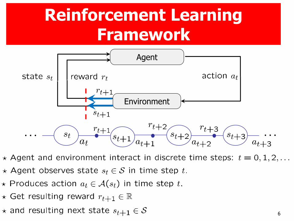
Reinforcement Learning Framework

. . . . . .

Agent

Environment

7

Markov Decision Processes

RL Framework + Markov assumption

8

Discount Rates

An issue:

Solution:

9

RL is different from Supervised/Unsupervised learning

10

State-Value Function

Bellman Equation of V state-value function:

Backup Diagram:

11

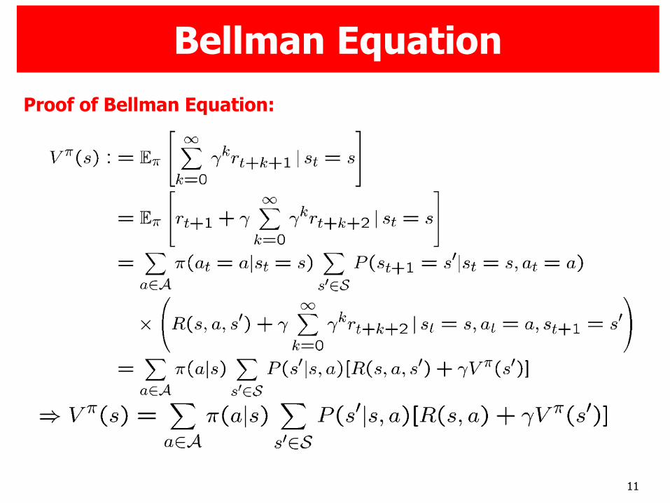
Proof of Bellman Equation:

Bellman Equation

12

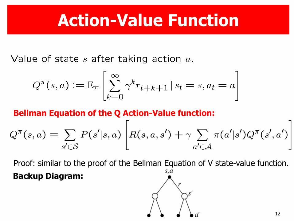
Action-Value Function

Bellman Equation of the Q Action-Value function:

Backup Diagram:

Proof: similar to the proof of the Bellman Equation of V state-value function.

13

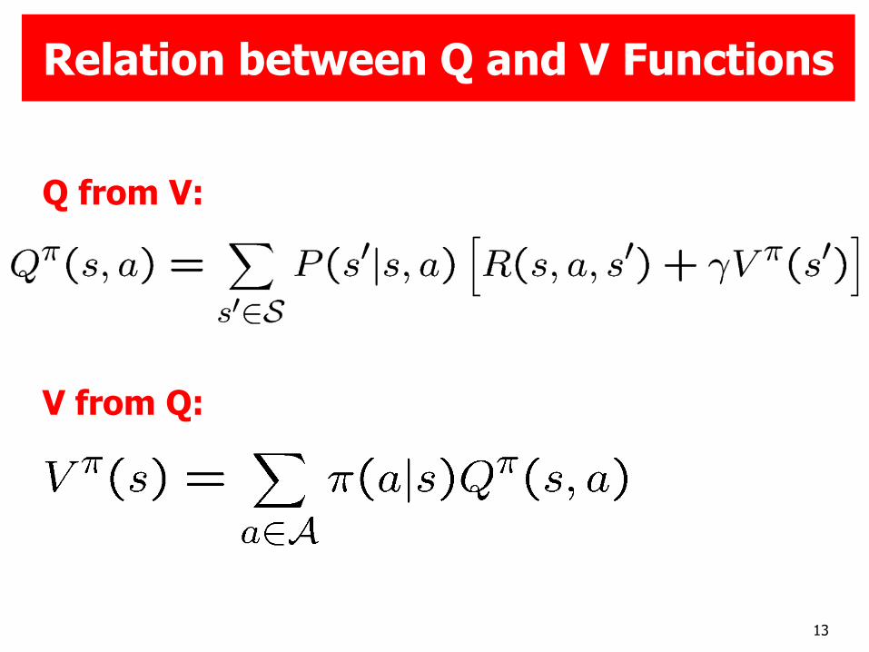
Relation between Q and V Functions

Q from V:

V from Q:

14

The Optimal Value Function and Optimal Policy

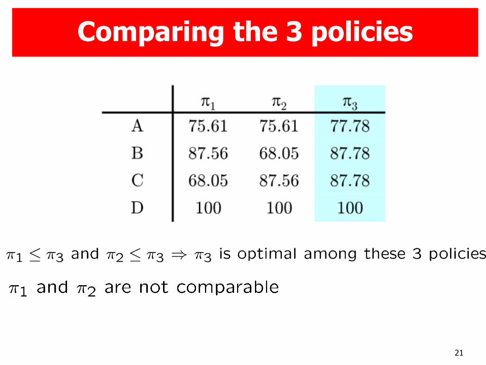
Partial ordering between policies:

Some policies are not comparable!

Optimal policy and optimal state-value function:

V*(s) shows the maximum expected discounted reward that one can achieve from state s with optimal play

15

The Optimal Action-Value Function

Similarly, the optimal action-value function:

Important Properties:

16

Theorem: For any Markov Decision Processes

The Existence of the Optimal Policy

(*) There is always a deterministic optimal policy for any MDP

17

Example

Goal = Terminal state

4 states

2 possible actions in each state. [E.g in A: 1) go to B or 2) go to C ]

P(s’ | s, a) = (0.9 , 0.1) with 10% we go to a wrong direction

18

Calculating the Value of Policy ¼

Goal

¼1 : always choosing Action 1

19

Calculating the Value of Policy ¼

Goal

¼2 : always choosing Action 2

Similarly as before:

20

Calculating the Value of Policy ¼

Goal

¼3 : mixed

21

Comparing the 3 policies

22

Theorem: Bellman optimality equation for V*:

Backup Diagram:

Bellman optimality equation for V*

Similarly, as we derived Bellman Equation for V and Q, we can derive Bellman Equations for V* and Q* as well

We proved this for V:

23

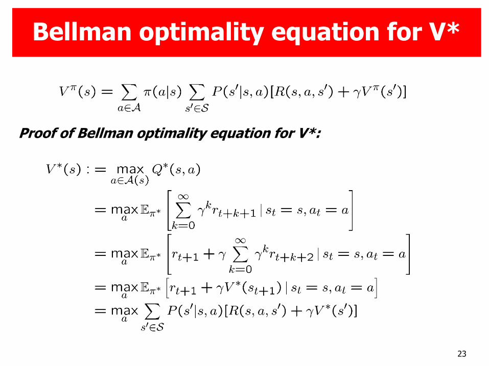
Proof of Bellman optimality equation for V*:

Bellman optimality equation for V*

24

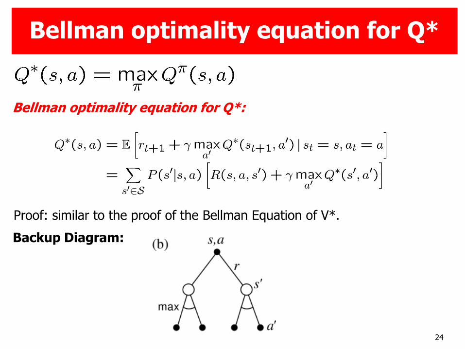
Bellman optimality equation for Q*:

Backup Diagram:

Bellman optimality equation for Q*

Proof: similar to the proof of the Bellman Equation of V*.

25

Greedy Policy for V

Equivalently, (Greedy policy for a given V(s) function):

26

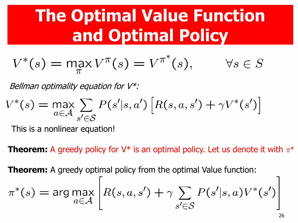
The Optimal Value Function and Optimal Policy

Bellman optimality equation for V*:

Theorem: A greedy policy for V* is an optimal policy. Let us denote it with ¼*

Theorem: A greedy optimal policy from the optimal Value function:

This is a nonlinear equation!

27

RL Tasks

Policy evaluation:

Policy improvement

Finding an optimal policy

28

Policy Evaluation

29

Policy Evaluation with Bellman Operator

This equation can be used as a fix point equation to evaluate policy ¼

Bellman operator: (one step with ¼, then using V)

Iteration:

Theorem:

Bellman equation:

30

Policy Improvement

31

Policy Improvement

Theorem:

32

Proof of Policy Improvement

Proof:

33

Finding the Optimal Policy

34

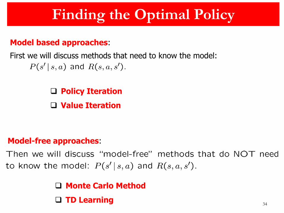
Finding the Optimal Policy

Policy Iteration

Value Iteration

Monte Carlo Method

TD Learning

First we will discuss methods that need to know the model:

Model based approaches:

Model-free approaches:

35

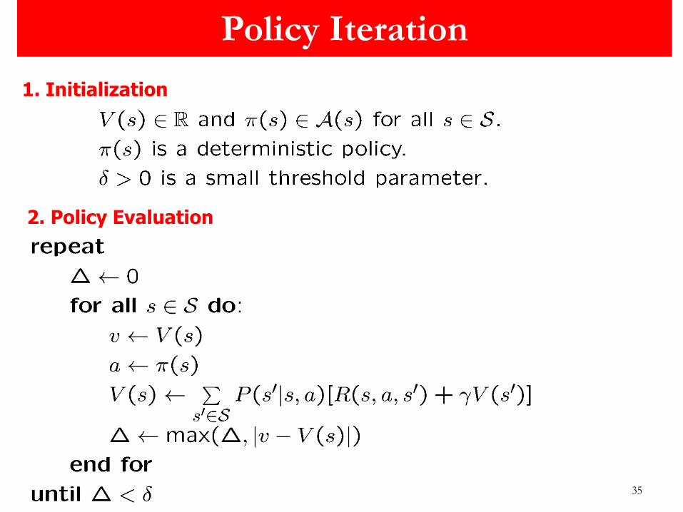
Policy Iteration

1. Initialization

2. Policy Evaluation

36

Policy Iteration

One drawback of policy iteration is that each iteration involves policy evaluation

3. Policy Improvement

37

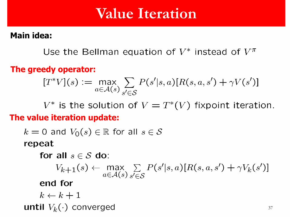
Value Iteration

The greedy operator:

Main idea:

The value iteration update:

38

Model Free Methods

39

Monte Carlo Policy Evaluation

40

Monte Carlo Policy Evaluation

Without knowing the model

41

Empirical average: Let us use N simulations

starting from state s following policy ¼. The

observed rewards are:

Let

This is the so-called „Monte Carlo” method.

MC can estimate V(s) without knowing the model

Monte Carlo Estimation of V(s)

42

If we don’t want to store the N sample points:

Online Averages (=Running averages)

Similarly,

43

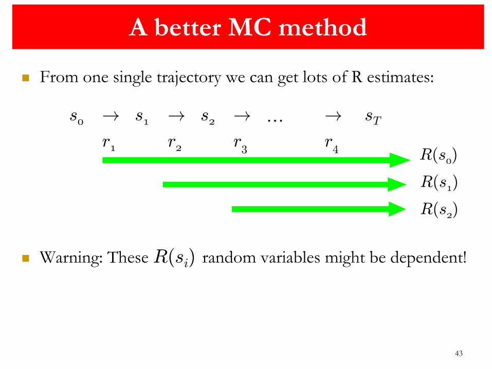
From one single trajectory we can get lots of R estimates:

Warning: These R(si) random variables might be dependent!

s0 ! s1 ! s2 ! … ! sT

r1 r2 r3 r4 R(s0)

R(s1)

R(s2)

A better MC method

44

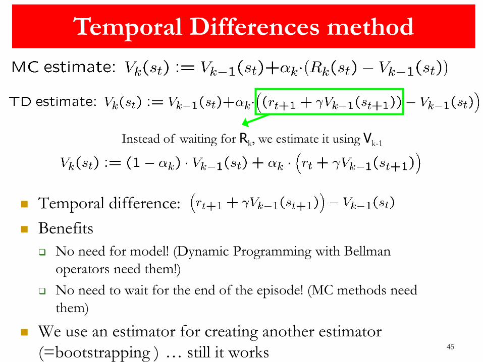
Temporal Differences method

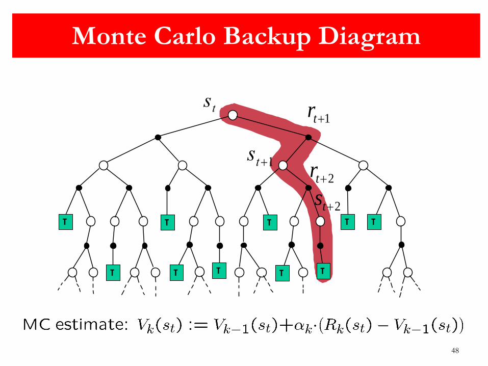
We already know the MC estimation of V:

Here is an other estimate:

45

Temporal difference:

Benefits

No need for model! (Dynamic Programming with Bellman

operators need them!)

No need to wait for the end of the episode! (MC methods need

them)

We use an estimator for creating another estimator

(=bootstrapping ) … still it works

Instead of waiting for Rk, we estimate it using Vk-1

Temporal Differences method

46

They all estimate V

DP:

Estimate comes from the Bellman equation

It needs to know the model

TD:

Expectation is approximated with random samples

Doesn’t need to wait for the end of the episodes.

MC:

Expectation is approximated with random samples

It needs to wait for the end of the episodes

Comparisons: DP, MC, TD

47

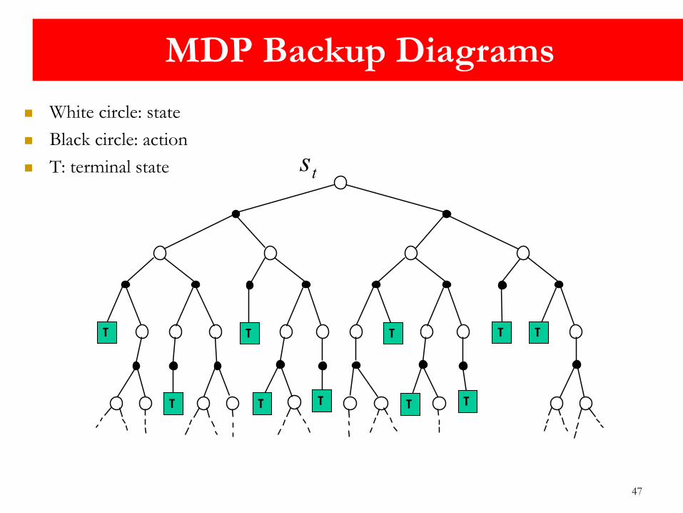
White circle: state

Black circle: action

T: terminal state

T T T T T

T T T T T

st

T T

T T

T T T

T T T

MDP Backup Diagrams

48

T T T T T

T T T T T

st

T T

T T

T T T

T T T

Monte Carlo Backup Diagram

1tr

st1

2tr

2ts

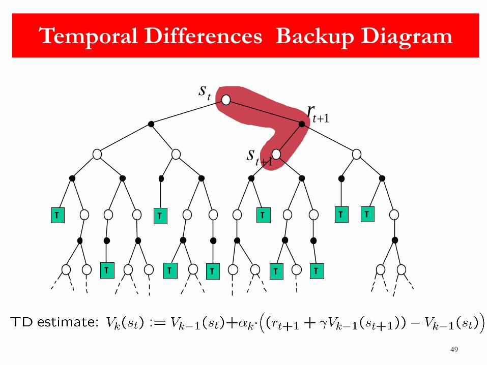
49

T T T T T

T T T T T

st1

1tr

T T T T T

T T T T T

Temporal Differences Backup Diagram

st

50

T

T T T

st

rt1

st1

T

T T

T

T T

T

T

T

Dynamic Programming Backup Diagram

51

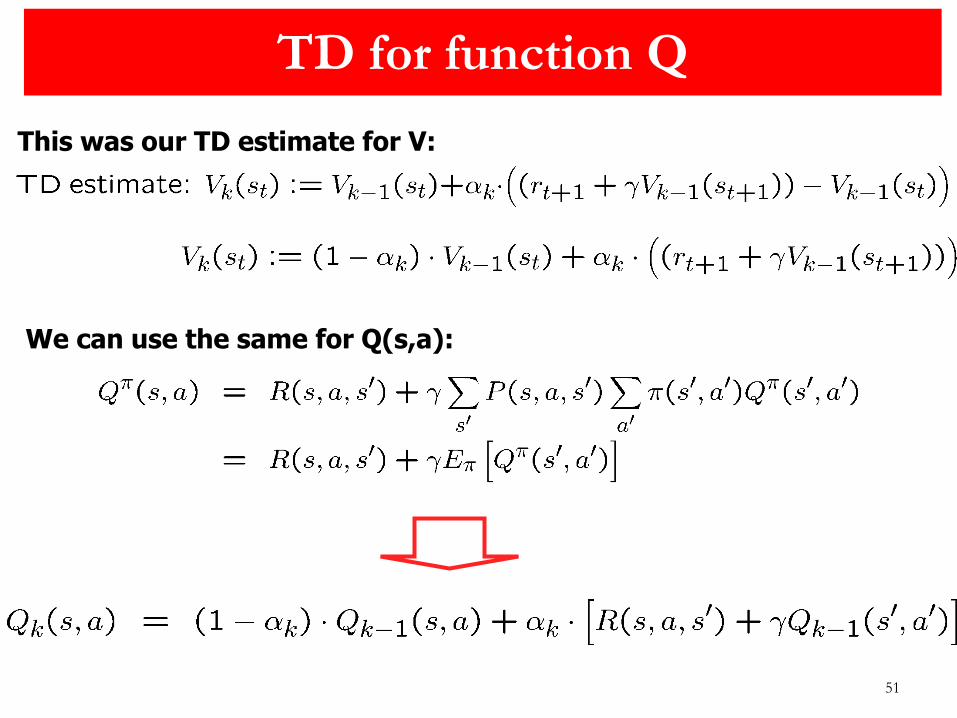
TD for function Q

This was our TD estimate for V:

We can use the same for Q(s,a):

52

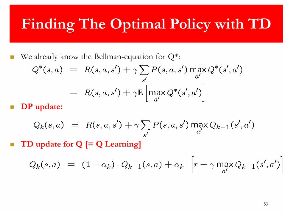
Finding The Optimal Policy with TD

53

We already know the Bellman-equation for Q*:

DP update:

TD update for Q [= Q Learning]

Finding The Optimal Policy with TD

54

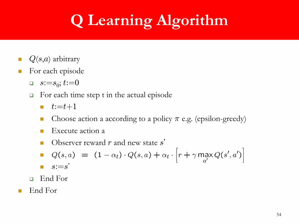
Q(s,a) arbitrary

For each episode

s:=s0; t:=0

For each time step t in the actual episode

t:=t+1

Choose action a according to a policy ¼ e.g. (epsilon-greedy)

Execute action a

Observer reward r and new state s’

s:=s’

End For

End For

Q Learning Algorithm

55

Q-learning learns an optimal policy no matter which policy the agent is actually following (i.e., which action a it selects for any state s)

as long as there is no bound on the number of times it tries an action in any state (i.e., it does not always do the same subset of actions in a state).

Because it learns an optimal policy no matter which policy it is carrying out, it is called an off-policy method.

Q Learning Algorithm