regulation, capital, and margining: quant angleecon.au.dk/.../andersen_quants_and_regulation.pdf ·...
TRANSCRIPT

Regulation, Capital, and Margining:Quant Angle
Leif Andersen
Bank of America Merrill Lynch
January 2014
Regulation, Capital, and Margining: Quant Angle – p. 1/143

Table of Contents - Part I
Overview of Regulation & Capital Basics
Regulation Overview
Capital Requirements for Market & Credit Risk
Market Risk Capital in a Nutshell + IRC/CRM
Economic and Regulatory Credit Risk Capital
Basel I and the CEM
Computation of Economic Capital for Loans
Non-Loan Portfolios
Basel 2 and the IRB
PD, LGD, and IMM
Regulation, Capital, and Margining: Quant Angle – p. 2/143

Table of Contents - Part II
IMM
EAD by Expectations
EPE
Reinvestment Risk and EEPE
Alpha multiplier
Effective Maturity
EE Computations
Computer Systems for EE
Appendix: Acronyms and Abbreviations
Regulation, Capital, and Margining: Quant Angle – p. 3/143

Table of Contents - Part III
Various Aspects of IMM
Basel 2 and 2.5 Flashback
Choice of Probability Measure
Backtesting
Carveouts
Margin Loans
Regulation, Capital, and Margining: Quant Angle – p. 4/143

Table of Contents - Part IV
Basel 3+4, Clearinghouses, IA/IM
Introduction to Basel 3
Non-Quanty Highlights of Basel 3
Changes to IMM and IRB
CVA VaR Add-On & Hedging
Clearing & Capital
Independent Amount
Basel IV overview
Regulation, Capital, and Margining: Quant Angle – p. 5/143

Table of Contents – Part V
Related Topics: “XVA”, Capital Management, Collateral,..
CVA/DVA
Symmetric and Asymmetric FVA
KVA, MVA
Management of Cost and Capital Metrics
Regulation, Capital, and Margining: Quant Angle – p. 6/143

.
I: Overview of Regulation& Capital Basics
Regulation, Capital, and Margining: Quant Angle – p. 7/143

Regulation and Quant/Strats - (1)
Just about the only "growth industry" in the banking world these daysis regulation-based: regulatory compliance and reporting, regulatoryexaminations, regulatory "optimization" (margins, collateral, CSAs,capital hedges, funding,...).
Fortunately, for quants/strats, much new regulation is complex and, forlarger banks at least, requires profound amounts of new analyticsdevelopment, documentation, and deployment.
While not revenue generating per se, these activities are very visibleat the top of the house, as capital numbers are typically in the$100BN’s, versus exotics trading book revenues in the $10MM’s.
Fees, charges, excess capital requirements, lawsuits,... are bigconcerns these days – and avoidance of them involve (shadow)revenues much larger than what quants typically work on.
Regulation, Capital, and Margining: Quant Angle – p. 8/143

Regulation and Quant/Strats - (2)
At BofA, regulatory compliance currently is more than 50% of thework the quant/strat group, and not likely to diminish.
We have launched significant learning programs to “reschool” quantsand to teach them capital basics.
Quants (including myself) are not meant to be regulatory experts(legal and capital groups have this responsibility), so the quant focusis necessarily selective and targeted to those areas that involveanalytics.
My "tour" of regulation is therefore highly biased in its coverage (andmy knowledge somewhat limited...)
Regulation, Capital, and Margining: Quant Angle – p. 9/143

Basel Reg Capital (and Margin)
Basel Committee on Banking Supervision (BCBS) is a Basel-basedcommittee tasked with developing international policy guidelines forbanking supervision, especially around capital adequacy
Founded by the Central Banks of the G10 countries in 1974. Currentmembers include most developed nations, such as Sweden. Denmarknot on the membership list!?
Role is to formulate broad principles, issued in documents availableon their web-site. It is up to the individual nations’ Central Banks(and/or other bodies, such as the FDIC and OCC in the US) to turnrecommendations into concrete regulation and supervision.
Currently, banks have to simultaneously (!) worry about 5 differentcapital adequacy accords: Basel 1, Basel 2, Basel 2.5, Basel 3, Basel4.
Regulation, Capital, and Margining: Quant Angle – p. 10/143

Dodd-Frank
The Dodd-Frank Act (which leans on Basel 3) was signed into law inthe US in July 2010. Based on a G20 agreement that means tostabilize the financial system through a variety of measures (clearing,transparency,..)
The part that is most relevant for Wall Street is Title VII ("Wall StreetTransparency and Accountability")
Subindex: centralized clearing, submission of derivatives data to acentral repository, SEFs, supervision through SEC and CFTC, Volckerrule, Collins floor.
The European "version" of the law is through EU directives: EuropeanMarkets and Infrastructure Regulation ("EMIR").
Regulation, Capital, and Margining: Quant Angle – p. 11/143

Capital for Market & Credit Risk - (1)
Capital is essentially a buffer that banks set aside to protect themfrom going insolvent when faced with losses.
These losses can come from market risk exposure – i.e., movementsin financial variables that affect the value of the bank’s holding ofsecurities.
Or these losses can come from counterparty credit risk exposure –i.e., from failures of the bank’s counterparties to pay on theirobligations.
As mentioned, capital adequacy regulations are written by agenciessuch as the Bank for International Settlements (BIS) and localregulators such the FRB, the FSA, etc. BIS drafts the so-called BaselAccords, the key methodology prescriptions.
Regulation, Capital, and Margining: Quant Angle – p. 12/143

Capital for Market & Credit Risk - (2)
From a regulatory standpoint, capital held by a bank is tiered intovarious “quality grades”.
Tier 1: Common Stock and Retained Earnings.
Tier 2: Supplementary bank capital that includes items such asrevaluation reserves, undisclosed reserves, hybrid instruments andsubordinated term debt.
Tier 3: “Everything else” – a greater number of subordinatedissues, undisclosed reserves and general loss reserves.
The regulatory formulas compute “RWA” – Risk Weighted Asset –values for both market risk (RWAM ), credit risk (RWAC), andoperational risk (RWAO).
Regulation, Capital, and Margining: Quant Angle – p. 13/143

Capital for Market & Credit Risk - (3)
The regulatory capital (RC) requirements then take the form
RC
RWAM + RWAC + RWAO≥ X% (1)
where X depends on the Accord: 8% for Basel 2, 10.5% for Basel 3.
There are also restriction on Tier 1 capital alone. Certain “globallysystemically important” banks (G-SIBs) need to post more Tier 1capital than other banks. BofA is on the black list.
I’ll ignore RWAO going forward.
Regulation, Capital, and Margining: Quant Angle – p. 14/143

Market Risk RWA in a Nutshell - (1)
Under regulatory capital rules, capital requirements for market riskexposure leans heavily on value-at-risk (VaR) computations,supplemented by add-on charges for so-called specific risk (=idiosyncratic event risk for individual firms).
These computations are fairly “standard”, involving 99th percentilereturn distributions over 10-day horizons.
Results can often be pulled from banks’ regular VaR market risksystems and the computations have traditionally not been complexenough to involve front office quants (they are generally handled byrisk management).
Regulation, Capital, and Margining: Quant Angle – p. 15/143

Market Risk RWA in a Nutshell - (2)
While our focus here shall be on credit risk capital, it is worth noticingthat the various financial crisis has caused BIS to recentlyrefine/revise its market risk capital requirements substantially.
Some of these changes has meant an increase in complexity that inmany banks has required implementation support by the quant teams.
In a nutshell, market risk requirement evolution is something like this:
Regulation, Capital, and Margining: Quant Angle – p. 16/143

Market Risk RWA in a Nutshell - (3)
Basel 1 (1988): RWA = 12.5 * m * VaR + specific risk add-on. Here,m = supervisory multiplier > 3.
Basel 2 and 2.5 (2004 and 2010): Add “stressed” VaR to overall VaRrequirement. For credit derivatives, add two new measures –Incremental Risk Charge (IRC) and Comprehensive Risk Measure(CRM) – to better measure risk associated with defaults and creditspread dynamics.
Basel 3 (2011): Add VaR on CVA (Credit Value Adjustment). Also,provisions for liquidity risk, leverage ratios, etc.
Basel 4 (draft): Replace VaR with CVaR, avoid double-counting VaRand “stressed VaR”, eliminate IRC/CRM,...
Regulation, Capital, and Margining: Quant Angle – p. 17/143

IRC/CRM - (1)
IRC (for CDSs) and CRM (for CDOs) were introduced following thefinancial crisis, which had regulators concerned about the effects ofcredit derivatives on financial stability.
BCBS appeared especially worried about lacking liquidity, and requireVaR-type calculations on a 1-year horizon.
In practice this requires simulation of *all* components that go intovaluation of structured credit derivatives books; enough samples toestimate the 99.9% confidence level.
This requires modeling of: joint dynamics of spreads, defaults,recovery, basis spreads, correlations, ratings, etc. Done by quants inmost banks.
Regulation, Capital, and Margining: Quant Angle – p. 18/143

IRC/CRM - (2)
The specification and implementation (and defense) of the simulationmodel and the portfolio “aging” assumptions was an expensive andlengthy exercise for most US banks.
AND NOW: Basel 4 eliminates these new charges (starting officially in2017).
Regulation, Capital, and Margining: Quant Angle – p. 19/143

Credit Capital - (1)
Regulatory credit risk capital : standardized regulatory requirementsfor how much capital banks should hold to protect themselves againstcounterparty defaults.
As mentioned, imposed by regulatory agencies such as BIS (Basel),FDIC, FRB, FSA, and so forth.
Economic capital : how much capital a firm should rationally set asideto protect against insolvency from economic credit losses, in theabsence of regulatory capital.
Economic capital is a risk measure (it does not equal actual capital setaside), and is used internally by banks for decision making purposes.
Regulation, Capital, and Margining: Quant Angle – p. 20/143

Credit Capital - (2)
In Basel 1, regulatory credit risk capital is computed in a verysimplistic fashion, based on deal notionals and categorization oftrades into various buckets. There is no explicit recognition of therating and recovery of the counterparty.
This rule, which is still the law in the US, is known as the CurrentExposure Method (CEM).
Regulation, Capital, and Margining: Quant Angle – p. 21/143

CEM Method - (1)
Consider a counterparty with several netting sets (NS). Trade j withthe counterparty is assumed to have value vj to the bank.
CEM method (Basel 1, 1988) writes RWA = 12.5 · EAD · RW, wherethe risk weight RW is given “in a table”, and EAD is
EAD = CE + PFE
Here CE (current exposure) is
CE =∑
k
∑
j∈NSk
vj
+
PFE (potential future exposure) is (Nj : notional of trade j)
PFE = (0.4 + 0.6 ·NGR) ·∑
∀jαjNj
Regulation, Capital, and Margining: Quant Angle – p. 22/143

CEM Method - (2)
Here net-gross ratio NGR is
NGR =CE
∑
∀j v+j
.
The αj are heuristic trade-level add-ons, to be looked up in tableprovided by BCBS. They depend on asset class and maturity.
Note that CEM, besides being quite heuristic, only recognizesmaximum 60% diversification
Regulation, Capital, and Margining: Quant Angle – p. 23/143
CEM Metnod - (3)
CEM has been criticized – even by BCBS itself – on many grounds,including (from BCBS docs):
It does not differentiate between margined and unmarginedtransactions;
The supervisory add-on factors do not sufficiently capture the levelof volatilities as observed over the recent stress periods; and
The recognition of hedging and netting benefits through NGR istoo simplistic and does not reflect economically meaningfulrelationships between the derivative positions.
Basel 2 was introduced in large part to address these issues and tomake regulatory credit capital more resemble economic capital.
Regulation, Capital, and Margining: Quant Angle – p. 24/143

Economic Credit Capital for Loans - (1)
Assume that a bank has a portfolio of loans with B counterparties.For counterparty i, the net loan notional is assumed to be Ni and theloss-given-default percentage (LGD) is li.
The primary economic risk of interest is here credit risk, due tocounterparty default exposure.
Over a period [0, T ], the cumulative economic loss due to defaults is
L(T ) =
B∑
i=1
Nili1τi≤T ,
where τi is the default time of counterparty i, and 1A is an indicator forthe event A (1 if A happens, 0 if it does not).
The expected value (in the actual probability measure P) of L(T ) isdenoted the credit reserve or the expected loss (EL).
Regulation, Capital, and Margining: Quant Angle – p. 25/143

Economic Capital for Loans - (2)
Hence, if E(·) denotes expectations in P,
EL = E(L(T )) =B∑
i=1
Nili · pi, pi = P (τi ≤ T ) ,
where pi is the default probability of counterparty i on [0, T ].
The credit reserve covering EL should be priced into the loans fromthe outset, and is not counted in economic capital. (Regulators dokeep an eye on whether banks have adequate provisions for EL).
Instead, economic capital is designed to sit as a buffer againstunexpected large losses.
Regulation, Capital, and Margining: Quant Angle – p. 26/143
Economic Capital for Loans - (3)
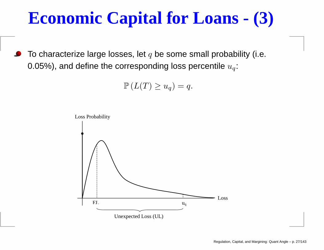
To characterize large losses, let q be some small probability (i.e.0.05%), and define the corresponding loss percentile uq:
P (L(T ) ≥ uq) = q.
Loss Probability
EL uq Loss
Unexpected Loss (UL)
Regulation, Capital, and Margining: Quant Angle – p. 27/143

Economic Capital for Loans - (4)
Economic Capital is set to protect against unexpected losses (UL), so
ECq = UL = uq − EL. (2)
For a given horizon T (often 1 year), a reasonable way to set q wouldbe based on historical default rates for a target rating or internal grade.
For instance, to reach an “AA” rating, one equates q to the T -yearhistorical default probability of AA-rated firms (≈ 0.03%, if T = 1).
With this amount of capital, the probability of credit losses wiping outall capital and reserves (and causing bank to go insolvent) wouldtheoretically equal a AA default probability.
Note: some ratings agencies rely on this principle to rate ring-fencedsubsidiaries. To be conservative, it is common to use a worst-caseanalysis on multiple horizons T .
Regulation, Capital, and Margining: Quant Angle – p. 28/143

Computation of EC - (1)
In principle, the computation of ECq in (2) can be done by MonteCarlo simulations, where we draw correlated default times for the poolof loan counterparties.
Default correlation is frequently generated with a one-factor Gaussiancopula. Specifically, if the copula correlation is ρ, we set
1τi≤T = 1Zi≤Hi, (3)
where
Zi =√ρX +
√
1− ρ ǫi,
X is a common Gaussian N(0, 1) economy-wide factor, and ǫi an i.d.N(0, 1) idiosyncratic random variable.
Regulation, Capital, and Margining: Quant Angle – p. 29/143

Computation of EC - (2)
In (3), we obviously need
P (Zi ≤ Hi) = P (τi ≤ T ) = pi,
or
Hi = Φ−1(pi),
where Φ(·) is the cumulative Gaussian distribution function.
With this, we can generate outcomes of 1τi≤T for all i, which allows usto simulate L(T ).
This, in turn, allows us to compute ECq from (2)
Regulation, Capital, and Margining: Quant Angle – p. 30/143

Large-Portfolio Limits - (1)
It is common to try to avoid Monte Carlo simulations by using variousapproximations or by (exact) Panjer recursions.
For capital computations, the most important technique is the simpleVasicek large-portfolio limit.
The assumption here is simple: there are an infinite number B ofcounterparties.
In this setup, consider the X-conditional expectation ofper-counterparty loss (L/B):
limB→∞
E(
B−1L(T )|X)
= limB→∞
B−1∑
NiliE (pi|X) ,
E (pi|X) = P (Zi ≤ Hi|X) = Φ
(
Hi −√ρX√
1− ρ
)
= Φ
(
Φ−1(pi)−√ρX√
1− ρ
)
Regulation, Capital, and Margining: Quant Angle – p. 31/143

Large-Portfolio Limits - (2)
We need some assumptions about the portfolio composition to allowus to form a meaningful large-B limit.
For instance, if the portfolio is homogeneous with all pi = p and li = l
identical, the limit exists and we get
limB→∞
E(
B−1L(T )|X)
= NlΦ
(
Φ−1(p)−√ρX√
1− ρ
)
= Nl · h(X).
In the homogeneous case, it is easily seen that
limB→∞
Var(
B−1L(T )|X)
= 0,
so in large-B limit, we diversify away all idiosyncratic risk notoriginating from X. And therefore we simply have:
limB→∞
L(T )/B = Nl · h(X).
Regulation, Capital, and Margining: Quant Angle – p. 32/143

Large-Portfolio Limits - (3)
We therefore have, for large B,
P (L(T )/B ≥ x) = P
(
h(X) ≥ x
Nl
)
= Φ
(
Φ−1(p)−√1− ρΦ−1
(
xNl
)
√ρ
)
(4)
We can compute ECq per counterparty as
ECq/B = uq − EL/B = uq − pNl,
where the percentile uq is given by P (L(T )/B ≥ uq) = q.
Using (4), we get the large-portfolio economic capital formula
ECq/B = Nl ·{
Φ
(
Φ−1(p)−√ρΦ−1(q)√
1− ρ
)
− p
}
. (5)
Regulation, Capital, and Margining: Quant Angle – p. 33/143

Non-Loan Portfolios - (1)
We emphasize that (5) is only an approximation of per-counterpartyEC, and does not (so far) cover anything other than loans.
We now up the ante and consider the more challenging situationwhere our exposure to a counterparty is not generated by loansalone, but by a complex portfolio of securities.
Let Vi(t) be the promised (default-free) time t value to the bank ofcounterparty portfolio i, and let Ci(t) be the (stochastic) collateralvalue posted by the counterparty.
The stochastic exposure at any t is (ignoring close-out risk, for now)
Ei(t) = (Vi(t)− Ci(t))+.
Unlike CVA, for capital we only consider the bank’s exposure tocounterparty (not vice versa).
Regulation, Capital, and Margining: Quant Angle – p. 34/143

Non-Loan Portfolios - (2)
Positive exposure combined with a default of counterparty i will leadto a credit loss of liEi(τi).
Therefore,
L(T ) =
B∑
i=1
liEi(τi)1τi≤T . (6)
This is similar to the loan setting from earlier, except that the loannotionals (Ni) are now random numbers (Ei).
Economic capital is still computed as before, ECq = uq −EL, but bothuq and EL are now more complicated to compute.
Regulation, Capital, and Margining: Quant Angle – p. 35/143
Non-Loan Portfolios - (3)
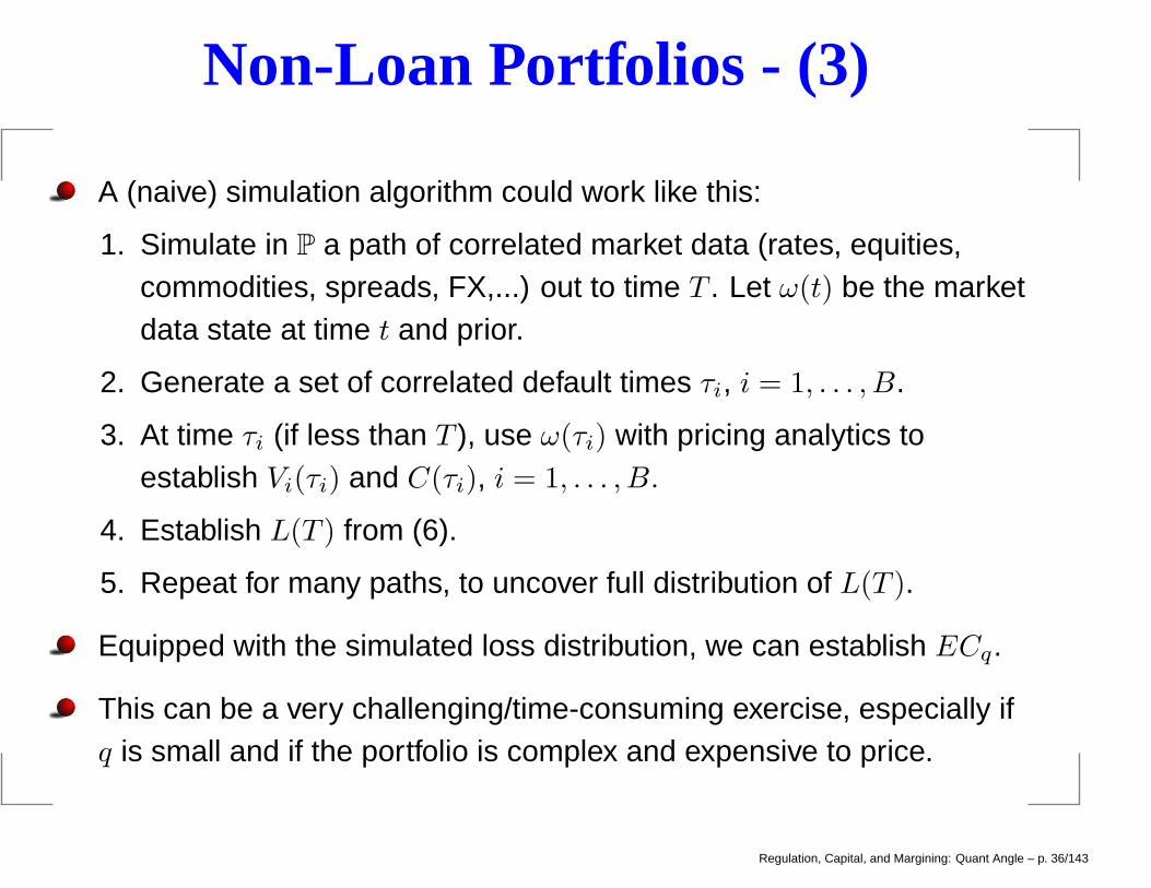
A (naive) simulation algorithm could work like this:
1. Simulate in P a path of correlated market data (rates, equities,commodities, spreads, FX,...) out to time T . Let ω(t) be the marketdata state at time t and prior.
2. Generate a set of correlated default times τi, i = 1, . . . , B.
3. At time τi (if less than T ), use ω(τi) with pricing analytics toestablish Vi(τi) and C(τi), i = 1, . . . , B.
4. Establish L(T ) from (6).
5. Repeat for many paths, to uncover full distribution of L(T ).
Equipped with the simulated loss distribution, we can establish ECq.
This can be a very challenging/time-consuming exercise, especially ifq is small and if the portfolio is complex and expensive to price.
Regulation, Capital, and Margining: Quant Angle – p. 36/143

Basel 2 and IRB - (1)
Key objective of the internal ratings-based methodology (IRB) inBasel 2 is to provide a framework for regulatory credit risk capital thatis spiritually similar to economic capital.
However, the IRB needs to be sufficiently simple and transparent tobe used in a regulatory setting.
A special requirement by regulators is portfolio invariance: the capitaltreatment given to a loan position with a given counterparty should beidentical from one bank to the next, and should not depend onexposure to other counterparties.
This is accomplished by assuming infinite diversification, in the samemanner as we did for the large-portfolio EC result.
Regulation, Capital, and Margining: Quant Angle – p. 37/143

Basel 2 and IRB - (2)
In addition, to avoid the complexities of joint market and defaultsimulations, regulators wish to decouple exposure and defaultsimulations by introducing the concept of loan-equivalent notional(LEN) a.k.a. exposure-at-default (EAD).
The idea behind EAD is to take a securities portfolio and replace it insome fashion with a simple loan. After this, the Vasicek formula forloans is applied directly.
We shall return to how EAD is computed later. Let us first discusssome modifications that Basel 2 makes to the Vasicek economiccapital formula (5).
Regulation, Capital, and Margining: Quant Angle – p. 38/143

Basel 2 and IRB - (3)
First, correlation is made a decaying function of default probability p,in an attempt to fit historical observations for asset correlations acrossvarious economic cycles. (???)
Second, regulators wish to introduce a component of transition risk,i.e. the risk of market value losses due to counterparty ratingsdeterioration (i.e. spread increases) over the interval [0, T ], even whenthere are no outright defaults.
Such transition risk increases with the spread duration of the portfolioexposure, so Basel 2 also needs a methodology for computing a loanequivalent effective maturity (M ). We discuss this later.
The transition risk adjustment to regulatory capital (RC) takes theform of a scale function k(M,p) that depends on effective maturity M
and default probability p.
Regulation, Capital, and Margining: Quant Angle – p. 39/143

Basel 2 and IRB - (4)
As in Basel 1, one writes RWAC = 12.5 ·RC where the key formula forregulatory capital (RC) for a counterparty-level trading position:
RCq = EAD ·RW, (7)
RW = l ·{
Φ
(
Φ−1(p)−√
ρ(p)Φ−1(q)√
1− ρ(p)
)
− p
}
· k(M,p) , (8)
and:
p: 1-year probability of default (PD);
l: loss-given-default percentage (LGD);
q: 0.001 (“once in a thousand years”);
M : effective maturity;
ρ(p) = 0.24− 0.12(1− e−50p) (ignoring small-firm terms)
Regulation, Capital, and Margining: Quant Angle – p. 40/143

Basel 2 and IRB - (5)
The transition risk adjustment function k is:
k(x, y) =1 + (x− 2.5)b(y)
1− 1.5b(y),
b(y) = (0.11852− 0.05478 ln y)2.
The function k is complex, and the way it has been arrived at is notcompletely transparent.
BIS documents hint at the usage of VaR computations using aratings-based MtM credit risk system similar to KMVPortfolioManager, but details are not disclosed. “Black Box”.
Regulation, Capital, and Margining: Quant Angle – p. 41/143

Basel 2 and IRB - (6)
The inputs to the RC computation in (7) are: EAD, LGD, PD, and M.
Because EL and UL emerge in a clean portfolio-invariant fashion fromobligor-specific characteristic (PD and LGD), the RC approach isconsidered purely ratings-based, hence the IRB moniker.
At most banks, a dedicated capital management team is responsiblefor the estimation of LGD and PD. The methodologies are actuarial innature, and must be approved by regulators.
The capital management teams are generally also responsible for theultimate reporting of RC numbers produced by (7).
However, it is becoming increasingly necessary to have quant teamsexecute the computations for EAD and M, a topic that we return toshortly.
Regulation, Capital, and Margining: Quant Angle – p. 42/143

FIRB vs AIRB
Depending on where EAD, LGD, PD and M come from, we have twoIRB approaches: Foundation IRB and Advanced IRB (FIRB and AIRB)
In FIRB, EAD is computed by CEM (see earlier slide) and LGD, M areprovided by regulatory rules. PD must be estimated by bank itself.
In AIRB, all quantities are provided by the bank itself, subject toexaminations (for each quantity separately) by regulators.
All large banks are expected to use AIRB.
Regulation, Capital, and Margining: Quant Angle – p. 43/143

PD - (1)
It would be tempting to pick PDs from traded securities, such asCDSs. Apart from the fact that such information is only available to avery small set of obligors, recall that we need default probabilities inthe actual probability measure P, not in a risk-neutral measure.
PD formally is:
“[T]he long-run average one-year default rate for the ratinggrade assigned [...] to the obligor, capturing the average defaultexperience for obligors in the rating grade over a mix ofeconomic conditions..”
Specialized risk rating teams at banks are charged with assigningeach counterparty to an internal obligor risk rating (ORR), an internalscale (e.g., from 1 to 10).
Regulation, Capital, and Margining: Quant Angle – p. 44/143

PD - (2)
Assigning an ORR to an obligor is often based on fundamentalanalysis (“scorecards”) similar to that undertaken by rating agencies.
In fact, rating agency ratings (when they exist), are taken into accountin the ORR, but supplemented by bank’s own data andmethodologies.
PD is not easy to estimate, and bank methodologies vary. There havebeen controversies, for instance (Risk Magazine, June 2013)
“Danske Bank and its regulator were pitched into openconflict in mid-June, when the Danish Financial SupervisoryAgency told the bank to hold more capital for corporate loans.[...] The primary driver of the seemingly anomalous risk weightsis the bank’s consistently low PD estimates, [...] although lowLGD numbers also play a role. ”
Regulation, Capital, and Margining: Quant Angle – p. 45/143

LGD
“A bank must estimate an LGD for each facility that aims toreflect economic downturn conditions where necessary tocapture the relevant risks. This LGD cannot be less than thelong-run default-weighted average loss rate given default [...]”
Regulators want banks to use LGDs that are higher than average, toreflect the fact that LGDs tend to increase in a systemic crisis. Can bedone by emphasizing data from periods where credit losses arehigher than normal.
“Downturn” LGDs are estimated by capital management teams usinghistorical default and recovery data.
The estimation often involves several factors, primarily the collateraltype and line of business.
Regulation, Capital, and Margining: Quant Angle – p. 46/143

EAD and M
The computation of EAD and M is governed by a regulatoryframework called internal models methodology (IMM) and is normallyhandled by a counterparty credit risk function, along with assistancefrom technology and, increasingly, front office quants.
EAD computations are complicated and model intensive, so bankshave to establish very robust controls and oversights around theircomputations.
In addition, rigorous backtesting procedures are required to prove thatthe models used for exposure computations are realistic andconservative. Models must be approved by model validation.
Formal submission to regulators and passing an examination with theOCC/FRB is required to be approved for IMM and Basel 2.
Regulation, Capital, and Margining: Quant Angle – p. 47/143

.
II: IMM
Regulation, Capital, and Margining: Quant Angle – p. 48/143

IMM & EAD Basics
Starting with EAD, the purpose of IMM is to find a way to take anarbitrary derivatives portfolio (including its collateral) and replace itwith a “representative” loan notional.
The loan notional need only be representative for a one-year period,since IRB works with this horizon.
The cumulative loss on [0, T ] generated for a portfolio V (t) withcollateral C(t) is
L(T ) = l · (V (τ)− C(τ))+1τ≤T = l · E(τ)1τ≤T , (9)
where τ is the counterparty default time and E(t) = (V (t)− C(t))+ isthe exposure at time t.
Regulation, Capital, and Margining: Quant Angle – p. 49/143

EAD by Expectations - (1)
If we only had a loan with notional N (and maturity > T ), we wouldhave
LN (T ) = l ·N1τ≤T . (10)
How do we pick N such that (9) and (10) are “close”?
We could try to align expectations (p is default probability, T = 1yr):
NE (1τ≤T ) = E (E(τ)1τ≤T ) ⇒ N =E(E(τ)1τ≤T )
p,
where we have assumed that l is non-random.
This can be rewritten as
N =E(E(τ)|τ ≤ T ) E (1τ≤T )
p= E(E(τ)|τ ≤ T ) . (11)
Regulation, Capital, and Margining: Quant Angle – p. 50/143

EAD by Expectations - (2)
In the computation of the r.h.s. of (11), it is clear that right- andwrong-way risk matters: conditioned on an early default (τ ≤ T ), is theexposure higher (wrong-way) or lower (right-way) than normal?
Building models that cleanly allow for dependence between exposureand τ is non-trivial, so regulators want a way out of this.
For this, suppose that exposure and τ are independent, in the sensethat
E (E(τ)|τ ≤ T ) =
∫ T
0
E (E(t))P (τ ∈ dt|τ ≤ T )
=
∫ T
0
EE(t)P (τ ∈ dt|τ ≤ T ) ,
where EE(t), t ≤ T , is the expected exposure profile.
Regulation, Capital, and Margining: Quant Angle – p. 51/143

EAD by Expectations - (3)
What can we make of the term P (τ ∈ dt|τ ≤ T )? In a simple Poissonmodel where default arrives at an intensity of λ, we have, for t ≤ T ,
P (τ ∈ dt|τ ≤ T ) =P (τ ∈ dt, τ ≤ T )
P ( τ ≤ T )=
P (τ ∈ dt)
P ( τ ≤ T )=
e−λtλ
1− e−λTdt.
If λ is smallish, we have
P (τ ∈ dt|τ ≤ T ) ≈ (1− λt)λ
λTdt ≈ 1
T.
So, therefore, with independence,
E (E(τ)|τ ≤ T ) ≈ 1
T
∫ T
0
EE(t) dt , EPE(T ). (12)
EPE (“expected positive exposure”) is the time-average of EE.
Regulation, Capital, and Margining: Quant Angle – p. 52/143

EPE
t 1 yr
EPE(1)
EE(t)
Note that EPE is an intuitive definition of loan-equivalent notional.
Regulation, Capital, and Margining: Quant Angle – p. 53/143

Reinvestment Risk - (1)
Combining (11) and (12) would suggest that a reasonable (andintuitive) estimate for EAD could be 1-yr EPE.
In reality, things are more complicated. First, we ignored wrong-wayrisk. Second, our principle of matching just the first moment wouldtend to ignore the volatility of the exposure, and could be less thanconservative. Third, we have ignored re-investment risk.
Implicit in the way we drew our exposure profile was an assumptionthat the portfolio is static: after time 0, we just leave it alone to ageand, ultimately, die.
For portfolios with maturities ≪ 1 year (e.g. repos, or short-dated FX),this is not conservative, since in reality the portfolio will be “refreshed”with new trades as part of the on-going trading business.
Regulation, Capital, and Margining: Quant Angle – p. 54/143

Reinvestment Risk - (2)
To capture this, Basel mandates that for RC computations one doesnot use the EE profile directly, but instead an alternative profile EE∗
(“effective EE”) that is found as a running maximum of the EE profile:
EE∗(ti) = max (EE∗(ti−1), EE(ti))
where {ti} is some sampling grid.
The time-average of this “modified” EE profile is called the effectiveEPE, or EEPE :
EEPE(T ) =1
T
∫ T
0
EE∗(t) dt.
If the longest deal maturity in the portfolio is less than T , then:
EEPE(T ) =1
Tmax
∫ Tmax
0
EE∗(t) dt.
Regulation, Capital, and Margining: Quant Angle – p. 55/143

Reinvestment Risk - (3)
t 1 yr
EPE(1)
EE(t)
EE*(t)
EEPE(1)
Note that EEPE > EPE. Not easy to justify EEPE formally, though.
Regulation, Capital, and Margining: Quant Angle – p. 56/143

Alpha Multiplier - (1)
What about the independence assumption and zero variance?
Originally, the Basel committee attempted to cover the missingvariance by replacing expected exposure (EE) by potential exposure(PE), where PE is, say, the 95th percentile of the exposure E(t).
This, however, was met with protests from industry whichdemonstrated (using simulation studies) that using PE would lead tolarge overestimates for economic capital. This is not surprising.
Instead, the Basel committee proposed to introduce a scale α > 1:
EAD = α · EEPE(T ) (13)
The “Alpha” multiplier is meant to adjust for a variety of effects:wrong-way risk, variance of the exposure, finite granularity ofportfolios, noise in E(t) simulation,...
Regulation, Capital, and Margining: Quant Angle – p. 57/143

Alpha Multiplier - (2)
Note: the original draft of Basel 2 (from 2001) had an explicitgranularity adjustment, which was subsequently dropped.
Industry studies on real portfolios have shown that α ≈ 1.1− 1.2.
Basel 2 uses α = 1.4, but does allow banks to argue for a lower α:
“Banks may seek approval from their supervisors tocompute internal estimates of alpha subject to a floor of 1.2,where alpha equals the ratio of economic capital from a fullsimulation of counterparty exposure across counterparties(numerator) and economic capital based on EPE(denominator), assuming they meet certain operatingrequirements.”
All things considered, α = 1.4 is probably reasonable.
Regulation, Capital, and Margining: Quant Angle – p. 58/143

But wait, there is more..
On top of the 1.4 multiplier, the BCBS has issued language to addanother fudge factor:
“The Committee believes it is important to reiterate itsobjectives regarding the overall level of minimum capitalrequirements. These are to broadly maintain the aggregatelevel of such requirements, while also providing incentives toadopt the more advanced risk-sensitive approaches of therevised Framework. To attain the objective, the Committeeapplies a scaling factor to the risk-weighted asset amounts forcredit risk under the IRB approach. The current best estimate ofthe scaling factor using quantitative impact study data is 1.06.”
???
Regulation, Capital, and Margining: Quant Angle – p. 59/143

Effective Maturity - (1)
IMM also covers the computation of effective maturity M .
M is meant to represent credit spread duration, so it makes sense toconsider a contract that pays out an amount EE(τ) at time τ , onsome interval [0, Tmax].
If the default intensity is λ, we have (ignoring discounting)
PV =
∫ Tmax
0
EE(t)λe−λtdt
such that, for small λ,
PV 01 =∂PV
∂λ=
∫ Tmax
0
EE(t)e−λtdt+ λ
∫ Tmax
0
EE(t)te−λtdt
≈∫ Tmax
0
EE(t) dt.
Regulation, Capital, and Margining: Quant Angle – p. 60/143

Effective Maturity - (2)
For a (loan) contract with a flat notional of EAD and maturity M , wewould have
PV 01 ≈ EAD
∫ M
0
dt = EAD ·M.
This suggests using (ignoring α)
M =
∫ Tmax
0EE(t) dt
EAD= T
∫ Tmax
0EE(t) dt
∫ T
0EE∗(t) dt
,
where Tmax is the longest maturity in the book, and T is 1 year.
Regulation, Capital, and Margining: Quant Angle – p. 61/143
Effective Maturity - (3)
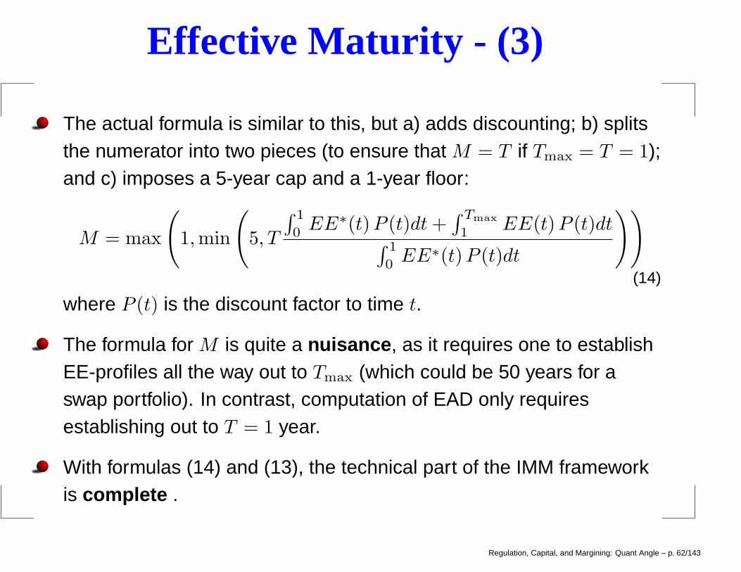
The actual formula is similar to this, but a) adds discounting; b) splitsthe numerator into two pieces (to ensure that M = T if Tmax = T = 1);and c) imposes a 5-year cap and a 1-year floor:
M = max
(
1,min
(
5, T
∫ 1
0EE∗(t)P (t)dt+
∫ Tmax
1EE(t)P (t)dt
∫ 1
0EE∗(t)P (t)dt
))
(14)
where P (t) is the discount factor to time t.
The formula for M is quite a nuisance , as it requires one to establishEE-profiles all the way out to Tmax (which could be 50 years for aswap portfolio). In contrast, computation of EAD only requiresestablishing out to T = 1 year.
With formulas (14) and (13), the technical part of the IMM frameworkis complete .
Regulation, Capital, and Margining: Quant Angle – p. 62/143

EE Computations - (1)
At the heart of both (14) and (13) lies the expected exposure profileEE – once this has been established, computation of EE∗ and, finally,EAD and M is straightforward.
Computation of EE is the biggest challenge of IMM.
Recall that
EE(t) = E(
(V (t)− C(t))+)
= E(E(t)) ,
where V is the (netted) portfolio value and C(t) the (dynamic)collateral.
Regulation, Capital, and Margining: Quant Angle – p. 63/143

EE Computations - (2)
A possible Monte Carlo algorithm looks like this:
1. Simulate in P a path of correlated market data (rates, equities,commodities, spreads, FX,...) out to time Tmax. Let ω(t) be themarket data state at time t and prior.
2. At some time-grid {ti}, use ω(ti) in pricers to establish value of all(netable) trades in the counterparty portfolio.
3. Aggregate trade values to compute portfolio value V (ti).
4. Use CSA and collateral data to establish C(ti). ComputeE(ti) = (V (ti)− C(ti))
+.
5. Repeat for many paths, to establish EE(ti), i = 1, . . . .
Regulation, Capital, and Margining: Quant Angle – p. 64/143

EE Computations - (3)
When simulating collateral, we should aim to incorporate “margindelay” when financially important.
Margin delays can mean two things: a) the frequency at whichmargin/collateral agreements get enforced; b) the delay associatedwith collateral disputes.
In the exposure simulation, one can explicitly account for a marginperiod η. Adding also at δ closeout period, exposure can be written assomething like max (V (t)− V (t− δ − η) , 0), for full collateralizationwith no thresholds.
Requires adding extra points to the simulation (to make sure that foreach ti we also have ti − δ − η). There are Brownian Bridge methodsavailable that can sometimes allow one to avoid doubling the grid.
Regulation, Capital, and Margining: Quant Angle – p. 65/143

Computer Systems for EE - (1)
Functionally, a system to compute EE profiles must have:
1. A representation of market data (rates, vols, spreads, equityprices, FX rates, etc.). Market data values at time 0 is the initialcondition for the market data simulation.
2. A simulation model for the joint evolution of the market data in thestatistical measure. Must be supported by historical back-testing.
3. A representation of trades. This representation must (unlike VaR)be able to correctly age trades through time.
4. Pricing models, taking market and trade date as inputs.
5. A concept of portfolios, netting sets, and collateral. Combined withthe trade data and pricing models, this allows for the computationof exposures on the simulation path generated by the statisticalmodel.
Regulation, Capital, and Margining: Quant Angle – p. 66/143
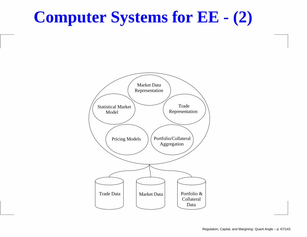
Computer Systems for EE - (2)
Statistical Market Model
Market Data Representation
Trade Representation
Pricing Models
Portfolio/Collateral Aggregation
Trade Data Market Data Portfolio & Collateral Data
Regulation, Capital, and Margining: Quant Angle – p. 67/143

Computer Systems for EE - (3)
In principle, it seems logical to use as many front office (FO)components for EE simulations as possible: FO market data, FOtrade data, FO pricing models, and so forth.
In practice, this may not be feasible due to enormous number ofrepricings that a capital system needs to perform.
For instance, if we simulate 1,000,000 trades (BAC has much morethan this) for 5,000 paths on a bi-monthly grid for 30 years, we need ofthe order of 1012 trade valuations (!).
Many security valuations are complex, so typically FO systems canonly handle in the order of 106 − 108 trades per day.
So strong simplifications are typically required on both traderepresentation, market data representation, and pricing models.
Regulation, Capital, and Margining: Quant Angle – p. 68/143

Pricing Errors - (1)
Simplifications can cause problems, if done too coarsely. This canhappen if price and/or data models are too simplistic, e.g., if theCapital systems get out of synch with FO developments.
A key symptom of problems are discrepancies in the current marketvalue (CMV) produced by FO and Capital systems.
To be more precise, let the counterparty portfolio in question consistof R trades with values v1(t), v2(t), . . . vR(t). That is,
V (t) =
R∑
j=1
vj(t)
Pricing errors cause (FO: front office; C: capital system)
V FO(0) 6= V C(0)
Regulation, Capital, and Margining: Quant Angle – p. 69/143

Pricing Errors - (2)
This causes initial exposures to differ, EFO(0) 6= EC(0). So, the EEprofile computed by the capital system has the wrong starting point.
Regulators like to measure pricing errors at the trade level, by addingabsolute trade pricing errors:
e =
R∑
j=1
|vFOj (0)− vCj (0)|
Regulators want a low value of e, which involves improving trade andmarket data fidelity, as well as improving pricing model precision. Verycomplex accuracy-efficiency tradeoffs are involved here
Also, some part of e is unavoidable, due to timing effects.
Regulation, Capital, and Margining: Quant Angle – p. 70/143
Pricing Errors - (3)
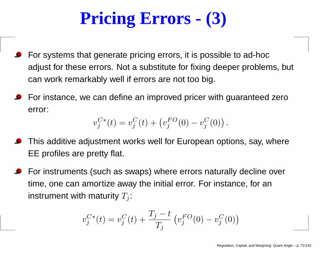
For systems that generate pricing errors, it is possible to ad-hocadjust for these errors. Not a substitute for fixing deeper problems, butcan work remarkably well if errors are not too big.
For instance, we can define an improved pricer with guaranteed zeroerror:
vC∗j (t) = vCj (t) +
(
vFOj (0)− vCj (0)
)
.
This additive adjustment works well for European options, say, whereEE profiles are pretty flat.
For instruments (such as swaps) where errors naturally decline overtime, one can amortize away the initial error. For instance, for aninstrument with maturity Tj :
vC∗j (t) = vCj (t) +
Tj − t
Tj
(
vFOj (0)− vCj (0)
)
Regulation, Capital, and Margining: Quant Angle – p. 71/143

Pricing Errors - (4)
t 1 yr
EE
alpha
EEC EEFO EEC (corrected)
Error correction procedure for a stylized swap.
Regulation, Capital, and Margining: Quant Angle – p. 72/143

But wait: the Collins floor
As part of the Dodd-Frank Act, US senator Susan Collins instituted afloor on capital that, in effect, makes sure that no future regulation willresult in less capital than what would have been required at the timeof passing the DF Act (July 2010).
Effectively, this floors all capital computations at Basel 1 capital levels.
So, after spending $100MM’s to implement the AIRB in Basel 2, theresult could be “thrown away” and replaced by a number thateverybody, including BCBS, agreed is less than meaningful.
According to the American Banker’s Association:
“Imposing a floor that is tied to Basel I rules raises thequestion of why any bank would want to undertake the expenseand effort to convert to the advanced approaches rules if it hasthe option not to do so. Such rules become, in essence, veryexpensive risk management exercises.”
Regulation, Capital, and Margining: Quant Angle – p. 73/143

IMM Appendix:
Acronyms and Abbreviations
Regulation, Capital, and Margining: Quant Angle – p. 74/143

Appendix - (1)
α: Basel 2 multiplier on EEPE, in computation of EAD
CCR: counterparty credit risk
CMV: current market value
EAD: exposure-at-default (a.k.a. equivalent loan notional, ELN)
E: random exposure profile
EC: economic capital
EE: expected exposure profile
EE∗: “effective” exposure profile (accounting for roll-over)
EEPE: 1-year time average of EE∗
EL: expected loss (a.k.a. credit reserve, CR)
Regulation, Capital, and Margining: Quant Angle – p. 75/143

Appendix - (2)
EPE: time average of EE
IRB: Internal ratings-based approach (Basel 2)
LGD: loss given default (percentage)
L: credit loss
M: effective maturity
PD: 1-year default probability
RC: regulatory capital
RW: risk weight on equivalent loan notional
RWA: risk weighted assets, RWA = RC * 12.5 (so RC = RWA * 8%)
UL: unexpected loss
Regulation, Capital, and Margining: Quant Angle – p. 76/143

.
3: Various Aspects of IMM
Regulation, Capital, and Margining: Quant Angle – p. 77/143

Basel 2 and 2.5 Flashback - (1)
Regulatory capital under Basel 2.5 is loosely broken into three pieces:
A general market risk piece (VaR + stressed VaR) and specific risk
IRC and CRM
Credit risk capital (the IRB and IMM)
We recall the Basel 2 Internal Ratings-Based (IRB) formula for creditrisk regulatory capital:
RC = EAD ·RW,
RW = 1.06 · l ·{
Φ
(
Φ−1(p)−√
ρ(p)Φ−1(0.001)√
1− ρ(p)
)
− p
}
· k(M,p),
Regulation, Capital, and Margining: Quant Angle – p. 78/143

Basel 2 and 2.5 Flashback - (2)
Where:
EAD: exposure-at-default (a.k.a. loan-equivalent notional);
p: 1-year probability of default (PD);
l: loss-given-default percentage (LGD);
M : effective maturity;
ρ(p) = 0.24− 0.12(1− e−50p);
k: function to incorporate transition risk.
IMM (Internal Models Methodology) is the regulatory framework forcomputing EAD and M .
A model for joint movements of all financial variables “in the world” areneeded to compute expected exposure (EE) profiles, and therebyEAD (which is 1.4·EEPE).
Regulation, Capital, and Margining: Quant Angle – p. 79/143

Choice of Measure - (1)
IMM models have to be validated by model validation and byregulators (FRB, OCC, FSA,..)
The model choice and parameterization is, rightfully, a key area offocus in IMM examinations
In theory, all simulations should be set in the actual (aka historical,aka real-life, aka statistical) probability measure.
Yet regulators allow for leeway:
“In theory, the expectations should be taken with respect tothe actual probability distribution of future exposure and not therisk-neutral one. Supervisors recognize that practicalconsiderations may make it more feasible to use the risk-neutralone. As a result, supervisors will not mandate which kind offorecasting distribution to employ.”
Regulation, Capital, and Margining: Quant Angle – p. 80/143

Choice of Measure - (2)
This leeway can be very substantial (probably more than regulatorsintended), since there is no such thing as a single risk-neutralmeasure – there is one for each choice of numeraire asset.
To demonstrate the effects of this, let us consider interest ratemodeling (an area of some tension).
Let f(t, T ) be the time t instantaneous forward rate to T , and assumethat a vector-valued Brownian Motion W (t) drives the forward curve.Let the (vector-valued) volatility for f(t, T ) be σf (t, T ).
By the HJM result, we know that in the actual measure P,
df(t, T ) = µ(t, T ) dt+ σf (t, T )⊤ dW (t)
µ(t, T ) = σf (t, T )⊤
(
∫ T
t
σf (t, u) du+ λ(t)
)
, α(t, T ) + σf (t, T )⊤λ(t)
Regulation, Capital, and Margining: Quant Angle – p. 81/143

Choice of Measure - (3)
Here λ(t) (market price of risk) is a vector-valued processindependent of T .
In the risk-neutral measure Q induced by using a rolling moneymarket account β = exp(
∫ t
0r(u)du) as numeraire, we have
µ(t, T ) = α(t, T ).
In the risk-neutral measure Q∗ induced by using a discount bondP (t, T ∗) maturing at time T ∗,
µ(t, T ) = α(t, T )− α(t, T ∗).
Range of allowable drifts is very large – in principle we can getµ(t, T ) = −∞ by setting T ∗ = ∞!
Regulation, Capital, and Margining: Quant Angle – p. 82/143

Choice of Measure - (4)
Also, since λ(t) is very hard to estimate historically, to boot there islarge uncertainty around the theoretically optimal drift.
All in all, drift terms of stochastic processes used for IMM should beset “pragmatically”. For example, it is not uncommon to setµ(t, T ) = 0: “roll up forward curve”.
Notice that for CVA applications, we are trying to price credit exposureso here there is no ambiguity, since
PV (t) = EQ
(
V (t)+1
β(t)
)
= EQ∗
(
V (t)+P (0, T ∗)
P (t, T ∗)
)
.
On the other hand, when computing expected exposure (rather thanpresent value of exposure)
EQ(
V (t)+)
6= EQ∗ (
V (t)+)
.
Regulation, Capital, and Margining: Quant Angle – p. 83/143

Choice of Measure - (5)
The drift ambiguity, and the use of expected exposure withoutdiscounting, are flaws in IMM.
In addition, there are several securities (e.g. compounding trades)where EQ(V (t)+) can be extremely large (overflow), whereas PV (t) isperfectly stable.
Ideally, one should have defined EE(t) = PV (t)/P (0, t).
Regulation, Capital, and Margining: Quant Angle – p. 84/143

Backtesting - (1)
Having covered drifts, how about variances (and co-variances)?
In theory, these are measure invariant and can often be constructedwithout ambiguity from observable option prices.
In practice, however, this is not what regulators want. Instead, theywant the choice of variances and co-variances to be based onhistorical data.
Mathematicians tend to be driven up a wall about this...
Determining whether a model is suitable for IMM is done throughbacktesting procedures.
In a nutshell, backtesting is the process of testing whether forecastsdone by a stochastic model match realized values.
Regulation, Capital, and Margining: Quant Angle – p. 85/143

Backtesting - (2)
For instance, for some risk factor X and some time grid {ti} we canconsider the collection of novations ǫij = X(ti +∆j)−X(ti) fori, j = 1, 2, . . ., where ∆j are time horizons.
The collection of ǫ·j for fixed j forms an empirical distribution that canbe compared by the distribution generated by a parametric model.
There is quite a bit of language around backtesting requirements inthe Basel rules, as well as a dedicated BIS publication exclusivelydealing with backtesting guidance (“Sound Practices for BacktestingCounterparty Credit Risk Models,” Basel Committee on BankingSupervision, December 2010).
Testing should be done at both the level of individual risk factors (e.g.,an FX rate) and over relevant aggregations, most notably through“representative portfolios”.
Regulation, Capital, and Margining: Quant Angle – p. 86/143

Backtesting - (3)
Per regulatory guidance, backtesting must:
Be done regularly as part of ongoing model performance measurement,and as part of ongoing model validation
Be subject to governance, especially w.r.t. to remediation of exceptions.
Test not only the potential exposure percentile but the whole distribution(e.g., 1%, 5%, 25%, 50%, 75%, 95%, 99%)
Test a representative sample of time horizons (∆j), incl. 1 year or more
Test correlations as well as volatilities
Be representative of the bank’s exposure
Monitor not only frequency of exceptions but also severity
Consider materiality of exceptions
Be designed with statistical significance in mind
Be based on historical calibrations using >3 years of data (Basel 3).
Regulation, Capital, and Margining: Quant Angle – p. 87/143

Backtesting - (4)
The complex (and thankless) task of calibrating and statisticallybacktesting models is normally handled by the credit risk team, ratherthan by banks. The models in questions have many 100s, if not1,000s of risk factors.
Often the statistical framework relies on a “cascade” of tests, startingwith BIS “traffic light” test.
Details are very much bank specific, so let us just describe the trafficlight test, the only concrete test that regulators have put forth.
Assume that our model predicts that ǫ falling outside some range H
takes place with probability q:
P (ǫ /∈ H) = q.
Regulation, Capital, and Margining: Quant Angle – p. 88/143

Backtesting - (5)
In a historical data series with n realizations, we can count therandom number of times N that ǫ is outside H (“exceptions”)
IF the model is correct, the distribution of N is (under suitableassumptions) binomial:
P (N = x) =
x
n
qx(1− q)n−x , B(q, x).
Suppose we use a cut-off of xc as a rejection of the model, in thesense that we will discard the model if N ≥ xc.
The probability of rejecting a correct model (a type I error) is
pI =∑
x≥xc
B(q, x).
Regulation, Capital, and Margining: Quant Angle – p. 89/143

Backtesting - (6)
IF the model is wrong, in the sense that really P (ǫ /∈ H) = w 6= q, theprobability of erroneously accepting a wrong model (a type II error) is
pII =∑
x<xc
B(w, x).
Based on tables with various values of q and w, BIS has come up withzones of outcomes for N that it considers green (all OK), yellow (couldbe a problem), and red (no good).
The BIS approach is quite simplistic, and really only done for lowvalues of q (1 %).
One would often supplement the traffic light tests with moresophisticated tests (Kupiec’s POF test, Jarque-Bera, Pearson Q, etc).
Regulation, Capital, and Margining: Quant Angle – p. 90/143

BofA Models and Simulation
Like most banks, BofA’s capital systems were built aroundcounterparty credit risk systems.
For IMM purposes, the models here are generally too simplistic, so aconvergence towards the CVA system has taken place.
Large parts of our CVA and IMM systems are merged, with a branchon the model configuration. CVA: market calibration (quants). IMM:statistical backtesting (quants, CCRA).
The resulting engine is effectively a large “what-if” machinery, and inprinciple could handle VaR and IA (through additional configurations).
Target state for most banks.
As the models deployed by BofA are not dissimilar to those used atDanske Bank, I will defer to tomorrow’s speaker for concrete details.
Regulation, Capital, and Margining: Quant Angle – p. 91/143

IMM Carveouts - (1)
For a variety of reasons, it is likely that some trades in a netting setwill not qualify for IMM treatment.
This can happen if there are no (or inadequate, in the sense of toohigh pricing errors) pricing models implemented on the IMM platform.
This, in turn, might be the case if an exotic security pricer is too slowto embed in the IMM simulation loop.
Note: exotic securities can often be priced efficiently usingregression-based methods, but these can take a while to develop,test, and validate – validation tends to be product specific. More onthis tomorrow..
In this case, it becomes necessary to split the portfolio in two pieces:one piece (V1) that is IMM compliant, and one piece (V2) that is not.
Regulation, Capital, and Margining: Quant Angle – p. 92/143

IMM Carveouts - (2)
V1 will attract credit capital according to Basel 2, and V2 will attractcredit capital according to Basel I (CEM). Total credit capital is thesum of the two contributions.
We notice that EE is always sub-additive when a portfolio and itscollateral is split:
EE(t) = E(
(V (t)− C(t))+)
= E(
(V1(t) + V2(t)− C1(t)− C2(t))+)
≤ E(
(V1(t)− C1(t))+)
+ E(
(V2(t)− C2(t))+)
,
if C(t) = C1(t) + C2(t) and V (t) = V1(t) + V2(t).
This is easily seen to carry through to EEPE and therefore to EAD. SoEAD is sub-additive.
Regulation, Capital, and Margining: Quant Angle – p. 93/143

IMM Carveouts - (3)
Note: when carving out trades, a concrete mechanism is required forsplitting the collateral. Normally a heuristic is needed, as there is nounique way to do this.
Is regulatory capital RC sub-additive? For this, we recall that
RC = EAD · f(l, p) · k(M,p) · 1.06
with f(l, p) being a prescribed function of LGD (l) and PD (p), andk(M,p) being a prescribed “transition risk” function of effectivematurity M and PD.
M depends on EE, so we must write, for the split portfolio,
RC1 +RC2 = f(l, p) · (EAD1 · k(M1, p) + EAD2 · k(M2, p)) ,
where we know that EAD1 + EAD2 ≥ EAD.
Regulation, Capital, and Margining: Quant Angle – p. 94/143

IMM Carveouts - (4)
Unfortunately, a careful analysis of the “black-box” function k revealsthat it has a design-flaw: it can depend on exposure profiles in such away that sometimes RC1 +RC2 ≤ RC. Basically a consequence ofthe cap that sits in the definition of M .
So regulatory capital is not always sub-additive: splitting the portfoliocan result in less capital.
While this might one doubt the coherence of the formulas, in practicestrict subadditivity virtually never happens.
Moreover, since the non-IMM portfolio gets subject to Basel 1 – whichis typically much more “expensive” than Basel 2 – splitting a nettingset involves a pretty severe capital cost.
In Basel 3 this penalty gets extremely high, as we shall see later.
Regulation, Capital, and Margining: Quant Angle – p. 95/143
Margin Loans - (1)
Securities that are subject to margin requirements are currently in alittle bit of a vacuum when it comes to regulatory capital.
One relevant business is margin lending, as executed in, say, theprime brokerage business. In the future most non-cleared securitieswill require margin posting. More about this later.
In margin lending, a client holds a portfolio of cash and securities withvalue π(t). Not all of this portfolio has been financed by the client; acertain amount of its value, D(t), has been lent to the client by thebank.
Writing π(t) = D(t) + E(t), the quantity E(t) is the client’s equity.
The lending bank can use the entire portfolio π(t) as collateral for itsloan D(t) if the client defaults. As long as E(t) > 0 the position isover-collateralized.
Regulation, Capital, and Margining: Quant Angle – p. 96/143

Margin Loans - (2)
To protect itself against the client not repaying the debt amount D(t),the lending bank has a policy where it will issue a margin call if theriskiness of the position is too high.
The call will require the client to top up the equity position with cash oreligible securities, to some level Emin(t).
Often, Emin(t) is set by VaR methods. Specifically, if we assume thatit will take a period of ∆ to liquidate the portfolio after a client default,we might want, for some small number q,
P (π(t+∆) < D(t)) < q,
or
P (X(t) > 0) < q, X(t) = π(t)− π(t+∆)− Emin(t)
Regulation, Capital, and Margining: Quant Angle – p. 97/143

Margin Loans - (3)
That is, the probability of the portfolio deterioration exceeding theequity over the liquidation horizon is very small.
Often q is minuscule – much less than 1%. Besides VaR protection,many margin policies add protection (through add-ons to VaR) againstdowngrades, concentration risk, liquidity issues, etc.
How do we define exposure for a margined portfolio?
If default takes place at time τ , first assume (worst-case) that theclient has no excess equity beyond the margin level Emin.
The loss to the lending bank associated with liquidation is
L(τ) = X(τ)+.
So, the expected exposure is EE(t) = E (X(t)+) .
Regulation, Capital, and Margining: Quant Angle – p. 98/143

Margin Loans - (4)
Since margined portfolios tend to be quite dynamic with active tradingand frequent margin calls, it is a challenge to predict what π(t) andEmin(t) will look like at time t. Some simplification is needed.
One (overly?) sophisticated method would involve using kernelregression to estimate conditional moments of the portfolio, and thento approximate the computation of VaR and, subsequently, Emin(t).
This calculation would assume that the current portfolio is “static’ ’andno new trades would ever be added. Often this is unreasonable –even though it is similar to regular IMM assumptions.
A better assumption for, say, prime brokerage is that the margin policyaims to keep the tail distribution of the loss-variable X close toconstant over time, in the sense that the VaR stays relatively fixed.
Regulation, Capital, and Margining: Quant Angle – p. 99/143

Margin Loans - (5)
Equivalently, assume that the current (t = 0) portfolio composition andmargin is a “representative” position.
With this assumption, we write for all t,
EE(t) = E(
X(0)+)
= E(
(K − π(∆))+)
, K = π(0)−Emin(0). (15)
So, to compute the entire EE profile (and thereby EEPE and EAD), we“just” need to price a put on π(∆).
One complication here is that K is very small due to theovercollateralization feature, so Monte Carlo simulation is difficult tomake operational without lots of tricks (importance sampling).
For speed and clarity, one can use delta-gamma approximations,coupled with a Gaussian distribution assumption for the risk factorsbehind π. Justified here due to the short time-horizon ∆.
Regulation, Capital, and Margining: Quant Angle – p. 100/143

Margin Loans - (6)
Specifically, we write
π(∆) = D⊤ǫ+1
2ǫ⊤Γǫ
where ǫ ∼ N(0, R) for some correlation matrix R.
After a few rotations, it is possible to write the characteristic functionfor π (∆) in closed form.
The expectation in (15) can then be written as a Fourier integral.
Due to the extreme OTM behavior of the integral, in practice we relyon saddlepoint techniques.
The saddlepoint techniques can be extended to provide efficienthedge and attribution analysis, which is very convenient in practice.(Joint work with J. Kim, 2012).
Regulation, Capital, and Margining: Quant Angle – p. 101/143

Margin Loans - (6)
It should be clear that capital requirements for margin business canbe very low. This might be controversial, and some elements of themargin portfolios may, for this reason, stay with Basel I throughcarve-outs.
On the other hand, regulators are generally skeptical aboutcherry-picking of accords, so we shall see.
Regulation, Capital, and Margining: Quant Angle – p. 102/143

.
IV: Basel 3/4, Clearinghouses,IA/IM
Regulation, Capital, and Margining: Quant Angle – p. 103/143

Introduction to Basel 3
Basel 3 was designed in 2010-2011, post crisis.
Basel 3 is a “mop-up” operation, that primarily aims to plug holes inBasel 2 that were revealed during crisis. Promote a more “resilient”banking system.
While banks in US have not yet gotten IMM approval, and have notyet moved to Basel 2, new rules for Basel 3 are already beingimplemented.
Originally planned for adoption in January 2013, most provisions inBasel 3 are delayed and will not become official standards for severalyears. Current projection: through 2019.
Regulation, Capital, and Margining: Quant Angle – p. 104/143

Some Non-Quant Elements of Basel 3
Raises quality of capital base, by eliminating Tier 3 capital andgradually increases proportion of Tier 1 capital (while still aiming for8% capital ratio).
Adds a 2.5% “capital conservation buffer” to be drawn on in times ofstress (to address procyclicality). Effective capital ratio is 10.5%.
Adds a non-risk weighted Tier 1 Leverage Ratio restriction of 3%, toavoid “excessive leverage in banking industry”.
Introduces various measures (Liquidity Coverage Ratio and NetStable Function Ratio) to address liquidity. LCR standard, say,ensures that there are liquid assets to completely cover net cashoutflows over a 30 day horizon. (Some quant element to this, actually).
Regulation, Capital, and Margining: Quant Angle – p. 105/143

Changes to IRB and IMM - (1)
EPE must now be computed with a model calibrated to a 3-yearstress period. “Stressed EPE”.
The maximum of the stressed and ordinary EPEs must be used inEAD computation.
The maximum is formed at the total capital level, not at thecounterparty level.
This results in a more conservative estimate, but not necessarily abetter capital measure.
Capital becomes increasingly insensitive to current market conditionsand might move in jumps.
Regulation, Capital, and Margining: Quant Angle – p. 106/143

Changes to IRB and IMM - (2)
For collateralized positions, the “close-out” period is lengthenedaccording to a new set of rules.
For many OTC derivatives positions, and for large netting sets (>5,000trades per quarter), the close-out period is lengthened from 10 to 20bdays. (Disturbingly “digital”).
However, for deals with a clearinghouse, 5 days is sufficient. Basel 3generally encourages trades with clearinghouses.
Another change to IRB approach: the asset correlations for financialfirms is increased by 25% for large financials as well as for allunregulated financials (hedge funds, say).
This addresses the fact that financial firms were seen to be moreexposed to systemic risk during crisis than non-financials.
Regulation, Capital, and Margining: Quant Angle – p. 107/143

CVA VaR Add-On - (1)
Recall that under Basel 2, capital is the sum of Credit Capital (IRB)and a variety of VaR, stress-VaR, and other charges (e.g., IRC, CRM).
During crisis, it was noted that a very large part of the variability ofbank earnings came from CVA/DVA charges due to moves in creditspreads: “2/3 of CCR losses were due to CVA losses, 1/3 due toactual defaults”.
In response, a CVA VaR charge has been added in Basel 3; it entersinto the credit risk RWA part of the overall computation.
The goal of this charge is to build a buffer against fluctuations incredit-worthiness of counterparties.
Probably double-counts something (like the ratings transition functionin the IRB)...
Regulation, Capital, and Margining: Quant Angle – p. 108/143

CVA VaR Add-On - (2)
Basel 3 always assumes that DVA=0. Reasonable to ignore self-creditwhen looking for metrics that test ability to avoid default. (Notreasonable from a MTM perspective, obviously).
Basel 3 defines CVA for a counterparty with known EE profile as:
CV A(0) = lM∑
n
(
e−sn−1tn−1/lM − e−sntn/lM)
×(
EE(tn−1)P (0, tn−1) + EE(tn)P (0, tn)
2
)
(16)
Here, lM is the market LGD (not the same as LGD used in IRB) andsn is the CDS spread observed in the market for tenor tn.
Uses the classical intensity approximation λ ≈ s/(1−R).
Notice that full EE profile to “longest trade” is needed, not just 1-yr.
Regulation, Capital, and Margining: Quant Angle – p. 109/143
CVA VaR Add-On - (3)
The collection of CVA charges across all N counterparties can beconsidered a function of N credit spread curves. Using a model forthese N curves (including correlation), one can compute the 10-day99% VaR originating from moves in the curves.
A regular as well as a stressed VaR number (using stressed EPEs)are to be computed. Both must be added to capital; the sum is a newcomponent of regulatory capital.
CDS (and index) hedges designated as CVA hedges can be includedin the computation (which will likely lower capital). One problem: MTMhedges will be different from capital hedges.
Worth reiterating: CVA VaR is not charged at the counterparty level,but is a firm-level measure.
Regulation, Capital, and Margining: Quant Angle – p. 110/143

CVA VaR Add-On - (4)
There are issues with the CVA VaR computation:
The Basel 3 definition of CVA is not how true CVA is actuallycomputed.
Focuses exclusively on the variability of credit spreads, but CVAdepends on many other risk factors. Hedges for these risks are leftnaked, giving wrong incentives.
CVA VaR should ideally not be separated out from regular VaRcomputations – this is not done for any other value component.
Why add stressed and non-stressed CVA VaR?
...
Regulation, Capital, and Margining: Quant Angle – p. 111/143

CVA VaR Add-On - (6)
From Risk Magazine, Oct 31, 2013:
“Critics of Basel 3’s credit valuation adjustment (CVA) capitalcharge have long warned it would produce perverse incentives.Now, in the form of a string of quarterly losses in Deutsche Bank’sCVA hedging programme, they believe they are being provedright.”
“How much should a bank pay to cut capital? [...] DeutscheBank has given some answers to that in recent quarterlystatements. In the first half of the year, the bank cut therisk-weighted assets (RWAs) generated by Basel 3’s charge forderivatives counterparty risk – or credit valuation adjustment(CVA) – from EUR28 billion to EUR14 billion.”
Regulation, Capital, and Margining: Quant Angle – p. 112/143

CVA VaR Add-On - (7)
“The hedging strategy that produced those savings also lostthe bank EUR94 million – a result of a mismatch between theregulatory and accounting treatments of CVA, which forces banksto choose which regime is most important. If a dealer chooses tohedge accounting CVA, it may not earn capital relief; if it choosesto mitigate the capital numbers, it may be stuck withprofit-and-loss (P&L) volatility.”
In the US, the Volcker rule in Dodd-Frank – and especially the recentlyreaffirmed ban on “portfolio hedging” – will likely make hedging ofCVA VaR illegal.
Recall that “portfolio hedging” is hedging that does not explicitlyinvolve risk mitigation of clearly identified trades.
Instrumental here: the “London whale” episode where JPM put on aseries of partial hedges to minimize the CRM charge.
Regulation, Capital, and Margining: Quant Angle – p. 113/143

CVA VaR Add-On - (8)
The CVA VaR charge is typically very large, often resulting in adoubling of capital relative to Basel 2. (!)
It is, in fact, so big that Basel 3 capital often exceeds Basel 1,meaning that the Collins floor often does not apply, at least forderivatives portfolios.
For trades carved out of IMM, Basel 3 requires that non-IMM nettingsets use the EAD as computed under CEM (not IMM) as a proxy forEE in (16).
This can be very expensive from a capital perspective, and provides astrong incentive to either simplify portfolios or to increase coverage toCVA systems to full-blown exotics.
One strategy for exotics: LS regression and a generic payofflanguage. Details left for tomorrow.
Regulation, Capital, and Margining: Quant Angle – p. 114/143

Basel 3: Clearinghouses - (1)
Recall that the idea of central clearing is to insert a clearinghouse, orCentral Counterparty (CCP), as a transaction intermediary:
End User Dealer ISDA
CSA
NO CLEARING
End User
ISDA or Customer Agreement
Clearing Member
Trade Ctpty Clearing Member
Clearinghouse Rules
Clearinghouse
CLEARING
Regulation, Capital, and Margining: Quant Angle – p. 115/143

Basel 3: Clearinghouses - (2)
Under the Dod-Frank law, the act of matching buyers and sellerspre-clearing must be done on a Swap Execution Facility (SEF).
SEF’s can loosely be thought of as electronic exchanges operating ona “many-to-many” basis. They operate centralized electronic tradingscreen on which market participant can post bids and offers foreverybody else to see – i.e., an “order book”.
A SEF may also offer a request-for-quote (RFQ) system whereparticipants can ask other market participants (at least 3) for quotes.
The SEF’s must report trades to a swap data depository (SDR) eitherfor real-time public dissemination or confidential regulatory use.
Regulation, Capital, and Margining: Quant Angle – p. 116/143

Basel 3: Clearinghouses - (3)
The CCP intermediates and settles P&L daily (variation margin), andhas no market risk. However, it will have close-out risk on default, so itwill insist on an additional buffer (initial margin).
Each CCP will have its own margin policies, and they often competewith each other on the specifics – especially on cross-margining.
Typically variation margin is settled in cash, whereas initial marginmight be in security form subject to CCP-specific hair cuts.
To avoid lowering standards, BIS has issued a number of documentsrelated to CCPs, including guidance to how CCPs themselves shouldbe capitalized (default fund waterfall approach) and charge initialmargin (5 days, 99%-ile).
There is guidance on how a CCP can become a qualifying CCP,which triggers lenient capital requirements for trading partners.
Regulation, Capital, and Margining: Quant Angle – p. 117/143

Basel 3: Clearinghouses - (4)
For Clearing Member (CM) exposure to an End User (EU), the CCPinitial margin requirements are always passed through to the EU, sothe exposure to the EU is small and of the same “overcollateralized”type as for prime brokerage. A similar “fixed upper tail” approach canbe used, along with usual IRB machinery. Or so we hope.
For EU or CM (“house account”) exposure to the CCP itself, the initialmargin sits only with the CCP, and is often considered by lawyers tobe at risk on a CCP default due to “co-mingling” of collateral. As such,the initial margin adds to the exposure – indeed, it is often the lion’sshare of the EAD.
More precisely, the EE to the CCP will be the sum of initial marginexposure and that of a regular collateralized position with no initialmargin (but with variation margin), for a 5-day close-out horizon.
Regulation, Capital, and Margining: Quant Angle – p. 118/143

Basel 3: Clearinghouses - (5)
If we can compute the EAD, how do we turn this into regulatorycapital? What PD/LGD/correlation/etc does one use for a CCP?
To understand the BIS capital guidance for CCPs, recall that underIRB for a regular counterparty:
RWA = 12.5 ·RC = EAD · 12.5 · f(l, p) · k(M,p) · 1.06
or
RWA = EAD ·RW (l, p)
where RW is a risk weight.
For trades with a qualifying CCP, one sets RWA = EAD · 2%, i.e. therisk weight is prescribed to be simply 2% – low, but not zero.
No CVA market risk charges for CCPs.
Regulation, Capital, and Margining: Quant Angle – p. 119/143

Basel 3: Clearinghouses - (6)
There are a large number of legal subtleties around CCPs and theexposures they generate to EUs and CMs. Some of this is covered inAndersen, L. (2013), “Exposure and Regulatory Capital:Clearinghouses,” BAC Technical Paper.
Here there are also attempts to build an approach to dynamicallymodel initial margin on the path, should the “fixed VaR” approach berejected in favor of the usual trade-aging IMM model.
The basic idea is to use a least squares or kernel regression toestimate the future distribution of portfolio moves over a ∆ period, andthen use a simple VaR approach to estimate margin. This can bescaled to ensure that the current (t = 0) margin is matched.
Also need to make assumptions/projections about the composition(bonds vs cash) of the initial margin.
Regulation, Capital, and Margining: Quant Angle – p. 120/143

Independent Amount - (1)
BIS in September 2012 issued a consultative document: “MarginRequirements for Non-Centrally Cleared Derivatives”. Rules weremade near-final in Feb 2013, to be implemented by 2015.
Proposal essentially is to require dealers to charge each other initialmargin (aka Independent Amount, or IA) for all non-cleared products.
Postings will, fundamentally, involve a third-party custodian, to preventhypothecation of margin (and to ensure its availability on default).
Controversial, since liquidity requirements can be enormous ( $1Trillion).
Following industry complaints, a threshold of EUR50MM wasinstituted below which margin need not be posted (BCBS242.pdf).Supposedly cuts liquidity req’s in half.
There are ample opportunities for disputes on margin. (BCBSrequires “agreement to common methodology” on transaction onset.)Regulation, Capital, and Margining: Quant Angle – p. 121/143

Independent Amount - (2)
ISDA is currently attempting to come up with an industry-wide“minimal methodology” document to at least set a floor under themargin requirements. SIMM: Standard Initial Margin Model.
The methodology will have to be simple, to make sure that all banks,large and small, can implement it easily
Delta-based VaR (either historical or parametric) is most likelycandidate.
Substantial work remains in defining the (factor-based, very likely)statistical reference models for all asset classes.
SIMM data model might be similar to what is used in NIMM (Not-IMM),with common factors as well as idiosyncratic risk components.
Capital can be computed by same methods as for margin loans.
Regulation, Capital, and Margining: Quant Angle – p. 122/143

Basel 4 - (1)
In 2012, the BCBS released a consultative document, "FundamentalReview of the Trading Book" (FRTB). This is known as Basel 4.
The FRTB acknowledges that rules have become unwieldy, costly,and difficult to regulate. Some proposals:
Replace all calibrations with stressed calibrations. Do not doublecount ordinary and stressed market risk RWA.
Replace VaR with CVaR/ES: ESα = E(X|X < V aRα).
Use different horizons for ES calculations to better reflect liquidityin various asset classes. From 10 days to one year.
Take steps to minimize the diversification benefits of IMM
Establish closer link between IMM and CEM methods, withCEM-type calculations being mandatory and possibly a floor.
NIMM ("Not IMM") methodology to replace CEM.
Regulation, Capital, and Margining: Quant Angle – p. 123/143

Basel 4 - (2)
Industry reception of FRTB has been quite mixed. For instance, DavidRowe in Risk Magazine (January 2014)
“One inappropriate innovation [...] is replacing VAR withexpected shortfall – the expected value of all losses greaterthan a specific threshold [...]. Besides adding little usefulinformation in practice, expected shortfall is impossible toback-test, since actual realised values are never observed.”
“Most disturbingly, it is now proposed that the revised, andnow highly complex, standardised approach must beimplemented by all banks, including those with approvedinternal models. It appears those behind the proposal have littleor no appreciation of how complex, costly and error-prone suchan effort would be. Hopefully [...] the Basel Committee will putthis idea where it belongs – on the regulatory scrapheap.
Regulation, Capital, and Margining: Quant Angle – p. 124/143

.
Related Topics: “XVA”, CapitalManagement, Collateral,..
Regulation, Capital, and Margining: Quant Angle – p. 125/143

CVA/DVA Basics - (1)
The incorporation of credit-related charges into market pricing is awell-established practice, supported by US accounting laws.
Consider a portfolio traded between the bank (B) and a counterparty(C). Let the portfolio have a no-default price of V0(t) to bank B.
Let the default times of B and C be τB and τC , respectively.
Assuming a universal recovery rate of R and the so-called marketquotation method (ISDA 1992) for default settlement, we write for thetrue value V (t) (assuming τB , τC > t):
V (t) = V0(t)− Et
(
(1−R)e−∫ τCt r(u) du V0(τC)
+1τC<τB
)
+ Et
(
(1−R)e−∫ τBt r(u) du (−V0(τB))
+1τB<τC
)
, V0(t)− CV A(t) +DV A(t).
Regulation, Capital, and Margining: Quant Angle – p. 126/143

CVA/DVA Basics - (2)
Both the CVA and DVA defined here are bilateral computations. Aunilateral (but incorrect) computation dispenses of the indicatorfunctions inside the risk-neutral expectations.
In a Cox process setting with intensities λB and λC we may write
CV A(t) = (1−R)Et
(∫ ∞
t
λC(u)e−
∫ ut(λC(s)+λB(s)+r(s)) ds V0(u)
+ du
)
DV A(t) = (1−R)Et
(∫ ∞
t
λB(u)e−
∫ ut(λB(s)+λC(s)+r(s)) ds (−V0(u))
+ du
)
.
Or, for the unilateral “version”
CV AU (t) = (1−R)Et
(∫ ∞
t
λC(u)e−
∫ ut(λC(s)+r(s)) ds V0(u)
+ du
)
DV AU (t) = (1−R)Et
(∫ ∞
t
λB(u)e−
∫ ut(λB(s)+r(s)) ds (−V0(u))
+ du
)
.
(17)Regulation, Capital, and Margining: Quant Angle – p. 127/143

CVA/DVA Basics - (3)
Traders generally dismiss the concept of DVA, as does the generalpublic (“Why do firms make money when their credit ratingdeteriorates??”). In particular, traders dislike the fact that they cannothedge their own spread.
Traders also don’t like bilateral CVA, for the same reason.
In addition, they dislike the fact that hedging bilateral CVA will cause amismatch with CCAR stress tests, which require unilateral definitions.
Same issue for the Basel 3 CVA VaR (although there are additionalissues here).
Tomorrow, we shall hear a lot about how to model and calculate thevarious forms of DVA and CVA in practice.
Regulation, Capital, and Margining: Quant Angle – p. 128/143

FVA - (1)
Besides CVA/DVA, the frictions that appear in world of regulation,margin, and expensive funding have led some (= traders) to suggest aplethora of new “valuation adjustments”.
The most common new measure is ‘funding valuation adjustment” –FVA.
This measure, which is quite controversial, is meant to measure the‘cost” of funding uncollateralized (or partially collateralized) positions.
To understand the notion, consider a trade where a bank’s treasuryissues an uncollateralized bond into the market, paying a coupon of c.
The full proceeds of the issuance is invested into a low-risk securitythat pays a coupon of d. Assume that the security cannot be financedin repo markets, but has a well-known market (auction) price, whichequals the price of the issued bond.
Regulation, Capital, and Margining: Quant Angle – p. 129/143

FVA - (2)
Since the security has lower risk than the issued bond, we would havec > d. The bank would “leak money” all the way to the default of thebank or to the maturity of the bond, whatever comes first.
Financial theory suggests that this is not a problem: the fact that c > d
is because there is a risk that the notional on the bank-issued bondwill not be paid back. Therefore, the “leakage” is just payment for thecash-flow that takes place at the default time of the bank.
From the perspective of the bank traders, however, their books willleak until the firm defaults, at which point they will loose their jobs. Sotrade is a bad one, from their perspective.
The equity holders of the bank will see it the same way: trade was abad one.
Regulation, Capital, and Margining: Quant Angle – p. 130/143

FVA - (3)
But the bond holders of the bank will be happy: at the time of defaultof the bank, they will have the purchased security in their possessionand will not have to pay back the (full) notional of the issued bond.
Market value = equity holder value + debt holder value. Total marketvalue impact of transaction is zero, but positive to debt holder andnegative to equity holders.
FVA adjustments takes a trader-centric view, and will insist that themarket value of the transaction is negative and therefore should notbe done. Effectively we are told to ignore the cash flow taking place atdefault because it won’t matter to traders.
Concretely, conjecture the existence of a universal funding curve foruncollateralized bank bonds. Let the rate earned on funds ber(t) + sF (t) at time t, for some spread s(t).
Regulation, Capital, and Margining: Quant Angle – p. 131/143

FVA - (4)
For an uncollateralized derivative with value V , the fundingcost/benefit over the period [t, t+ dt] is interpreted by traders to be−V (t)sF (t) dt. Taking this at face value it is tempting to define afunding valuation adjustment (FVA) of
FV A(t) = −Et
(
∫ T
t
e−∫ ut
r(u)V (u)sF (u) du
)
.
Assuming that V represents the value of a European payout at time T,
and adding the funding cost/benefit to the value of the payout, we get(using Feynman-Kac or the dividend formula)
V (t) = Et
(
e−∫ Tt
r(u) duV (T ))
+ FV A(t)
= Et
(
e−∫ Tt
(r(u)+sF (u)) duV (T ))
.
Regulation, Capital, and Margining: Quant Angle – p. 132/143

FVA - (5)
So basically, all uncollateralized derivatives should be discounted at ahigher discount rate. (Piterbarg (2011))
One immediate issue: derivatives have different values for differentfirms, and the market will not clear!
Another issue: for securities where the counterparty owes us money(when V (T ) is positive), we end up discounting by our spread, ratherthan with the spread of our counterparty. When CVA is later added(which traders still want to do), we double-count.
A third issue: for securities where the counterparty is owed money(when V (T ) is negative) FVA and unilateral DVA will be about thesame, so we will double-count unless we turn off DVA. (See (17).)
Regulation, Capital, and Margining: Quant Angle – p. 133/143

FVA - (6)
To at least avoid the overlap with DVA, some researchers define FVAas an asymmetric metric:
FV A∗ = Et
(∫ ∞
t
sF (u)e−
∫ ut
sF (s) dse−∫ ut
r(s) dsV (u)+ du
)
.
This metric can no longer be applied at the trade-level, only toportfolios. It effectively assumes that excess funds is an unstablesource of funding and will only earn interest at OIS.
There is great controversy around the topic of FVA. Academicsdisregard it, traders love it.
At the moment, unclear who is getting the upper hand, but yesterday’sJPM report shows that FVA is showing up in accounting statements:
Regulation, Capital, and Margining: Quant Angle – p. 134/143

FVA - (7)
From www.libertyinvestor.com, January 14, 2014:
“The biggest surprise in JPM’s Q4 earnings release was notthe firmâAZs legal troubles: those are well-known [...] No, thebiggest surprise by far was that as of this quarter in addition toits trusty use of DVA or a Debt Valuation Adjustment (the oldfudge when a bank “benefits” when its credit spreads blow out)JPM also added the use of a Funding Valuation Adjustment orFVA. The amount of the FVA benefit? A whopping USD1.5billion add-back to GAAP EPS, which together with DVA,resulted in a USD2.0 billion pretax loss [...] ”
Looking at JPM’s statement, it appears that they are using theasymmetric version of FVA – and only charge for receivables.
JPM claims that they see evidence in market prices for FVAadjustments.
Regulation, Capital, and Margining: Quant Angle – p. 135/143

FVA - (7)
My opinion: FVA is a useful decision metric (it is roughly a measureof “shareholder value”), and can be used to screen trades to see ifthey benefit share holders.
It is not a properly defined measure of market value , but potentially auseful measure to minimize. Should be FVM, not FVA.
Current accounting laws, to my reading, do not support FVA and anyother “entity specific” cost allocation into a market price. “Marketvalue” is not the same as “production cost”.
Of course, if every firm started using FVA, the auction principles ofaccounting laws would suggest a “minimum funder” valuationadjustment. This could differ significantly from FVA and would besimilar to a classic asset-specific liquidity adjustment.
Regulation, Capital, and Margining: Quant Angle – p. 136/143

KVA - (1)
Suppose that a trade (or group of trades) is deemed to be associatedwith a regulatory capital amount of C(t). The capital amount varieswith time, dependent on the exposure generated by the trade overtime.
Equity holders that put up capital want a (high) returnrE(t) = r(t) + sE(t) on their investment.
Like for FVA, we can define a k(c)apital valuation adjustment, KVA, tocapture the “cost” of having to put capital against a position:
KV A = −E
(
∫ T
0
e−∫ t0r(u) duC(t)sE(t) dt
)
.
Regulation, Capital, and Margining: Quant Angle – p. 137/143

KVA - (2)
The main complication here is the fact that future capital C(t) isdifficult to simulate: we need to be able to do a full capital computationat each point in the future.
And to see the marginal cost impact of a new trade, we need to runtwo simulations: with and without the trade.
For credit capital, we need to execute something like (simplified a bit)
C(t) = RW (p, d) · 1.4 · EEPE(t, t+ δ) · 1.06
where RW is a risk weight computed by the Vasicek large-portfolioresult, δ = 1, and (V is the portfolio value)
EEPE(t, t+ δ) =1
δ
∫ t+δ
t
maxs∈[t,u]
Et
(
V (s)+)
du.
Regulation, Capital, and Margining: Quant Angle – p. 138/143

KVA - (3)
But how do we compute Et(V (s)), s > t, for some future time t? A“simulation within a simulation” is normally too expensive.
A typical approach involves writing
Et
(
V (s)+)
= E(
V (s)+|Ft
)
≈ E(
V (s)+|V (t))
There are standard methods for estimating this quantity, either byleast-squares regression, or by kernel regression methods.
For the latter, when doing the expectation of E(X|Y ) we can rely onthe following n-sample estimator (Nadaraya-Watson kernel estimator)
E(X|Y = y) ≈∑n
i=1 Xi ·K(
Yi−yh
)
∑ni=1 K
(
Yi−yh
)
Regulation, Capital, and Margining: Quant Angle – p. 139/143

KVA - (4)
Here K is a measure of “closeness” known as a kernel. h is asmoothing parameter known as the bandwidth.
Technically, a kernel is just a real function satisfying∫ ∞
−∞K(x) dx = 1, K(x) = K(−x).
Gaussian: K(x) = e−x2/2√2π
. Uniform: K(x) = 121x∈[−1,1]. Epanechnikov:
K(x) = 34
(
1− x2)
1x∈[−1,1].
The bigger h is, the smoother (and less noisy) the kernel regressionestimate becomes. But a big h also implies a big bias.
A low h will give noisy, but less biased, results.
Regulation, Capital, and Margining: Quant Angle – p. 140/143

KVA - (5)
There are rules for picking a good h that gives a good compromisebetween noise and bias. For instance, for the Gaussian kernel,
h ≈ 1.06 · n−1/5 ·√
Var (Y )
Even if we can pull of a good estimation, there are considerablepractical obstacles in the KVA concept. F.ex.:
Capital is computed at the portfolio level, not the trade level.
How do we estimate the “cost of capital/equity”?
How do we project changes in Basel accords? And Basel 6, 7, 8,..
What about the other elements of regulatory capital (VaR, CVA Var(Basel 3), maturity adjustment, etc.)?
And we can also define “XVA“ adjustments for other frictions, such asinitial margin – MVA anybody?
Regulation, Capital, and Margining: Quant Angle – p. 141/143

How to manage all this??
In this talk, we have outlined a (very) large range of regulatoryrequirements that are introduced through regulation and throughfunding imbalances.
Many of these impact the bottom line, directly or indirectly.
While regular quants produce the numbers, there is now increasinglythe need for another function: capital structurers/strats.
Here, the problem is how to manage around all the capital and marginrequirements in a rational/optimal way.
Increasingly this is done by a central desk in the bank, typically insidethe CVA trading group.
Supported by diagnostic tools: where areexposures/capital/margin/liquidity coming from?
Regulation, Capital, and Margining: Quant Angle – p. 142/143

Management
This is a new function, but an important one
Tools in quiver include:
Trading on multiple CCP venues in optimal manner (to minimizemargin)
Merging legal entities (to compactify netting sets)
Intermediation/novation
Innovative CSAs that the clients can tolerate (e.g., caps onpostings)
Trade consolidation/compression
There is a lot more to come (and say) in this space, I’m sure..
Regulation, Capital, and Margining: Quant Angle – p. 143/143