Regulating Child Care: The Effects of State Regulations onChild Care Demand and Its Cost*

by

V. Joseph HotzUniversity of Chicago

and

M. Rebecca KilburnRAND

First Draft: May 1994Revised Draft: October 1996

*This research has been supported, in part, by the Institute for Research on Poverty under a contractfrom the Department of Health and Human Services. We wish to thank David Blau for providing uswith data on state child care regulations and for helpful comments on a previous draft of this paper.We also wish to thank Mike Brien for help in preparing the NLS72 files, and Kevin Murphy, Hec-tor Cordero-Guzman, Tom Mroz, and Jacob Klerman for providing us with tabulations from theCPS. This paper also benefited from the comments received from workshop participants at theUniversities of Chicago, Wisconsin-Madison, Virginia, and Rice and Texas A&M and Duke Uni-versities and the U.S. Bureau of Labor Statistics.

Abstract

In this paper, we examine the effects of existing state-level child care regulations on thecost, or price, of non-parental child care, the demand for (non-parental) child care by parents, andthe mother’s decision to enter the labor force. We distinguish between the indirect effects of regu-lations on demand via their effect on the cost of such care facing parents as well and the direct (andnon-price) effects regulations may have by imposing standards in the form of minimum levels ofquality on available care facing parents. In our empirical analysis, we analyze the child care deci-sions of all parents with preschool age children, including households with working and non-working mothers, using child care data from the 1986 wave of the National Longitudinal Survey ofthe High School Class of 1972 (NLS72). We present estimates of the effects of two sets of regula-tions—namely, restrictions on child-to-staff ratios in day care centers and educational and/or train-ing requirements of workers in either centers or home day care setting—as well as two types ofchild care subsidies—child care tax credit for working mothers and subsidies to providers—on thechild care and maternal work decisions of households as well as on the hourly cost of child care.Our evidence indicates that state regulations both increase the cost of child care as well as have di-rect (non-price) effects on utilization but that their total effect tends to reduce the utilization of mar-ket-based child care, especially among households with non-working mothers. Since economicallydisadvantaged and black women are disproportionately represented in the latter group, it appearsthat one of the consequences of regulations are to deter the utilization of child care by householdswith children for whom the purported developmental benefits of organized day care might be mostbeneficial.

1

1. Introduction

Over the last two decades, the United States has witnessed a substantial growth in the child

care market, fueled, in large part, by the rise in the labor force participation rates of married women.

For example, Hofferth and Phillips [1987] estimate that the use of center-based care by full-time

employed mothers with children under 5 years of age grew by almost 50% over the five-year period

from 1977 to 1982 and, according to statistics from the U.S. Department of Education, the percent-

age of 3 and 4 year-olds enrolled in some sort of preschool program (such as nursery schools or

Head Start programs) grew from 5% and 16%, respectively, in 1965 to 29% and 49% in 1985.1

Consistent with these trends, the number of persons employed in child care has grown faster than

has overall employment in the U.S. economy.2

The growth of the child care market has resulted in an increased interest in and debate about

the need for governmental regulation of child care services. While most states already regulate

some aspects of child care services, child care advocates have pressed for the imposition of more

stringent regulations of these services and their standardization across states by the federal govern-

ment. Their case for imposing minimum standards on child care services appears to be based on

one or more of the following arguments: (1) the potential for irreparable harm by exposing children

to low-quality child care services, (2) the difficulty that parents may have in evaluating such serv-

ices due to informational problems which characterize child care markets, and (3) the potential un-

derprovision of parental-determined child care due to the externalities associated with children.

Child developmental specialists argue that exposing young children to child care environ-

ments that are unhealthy or unsafe, to arrangements in which children may be abused, or to those

which fail to provide young children with adequate developmental stimulation can have pernicious

1 U.S. Department of Education [1986].

2

and irreparable effects on children’s long term cognitive, emotional and social development.3 To

the extent that such effects are irreparable, obtaining ex post compensatory relief for exposure to

low-quality child care services through the courts is an unsatisfactory option for parents (or chil-

dren). The imposition and enforcement of minimum standards on available child care services pre-

empt the possibility of such harm being inflicted on children by eliminating low-quality child care

services.

The lack of perfect information faced by consumers in the child care market has also been

cited as a justification for legislating minimum quality standards and the licensing of day care pro-

viders. Parents may be imperfectly informed about the quality of available care because the multi-

dimensional attributes of these services are difficult to evaluate and/or monitor.4 Informational

asymmetries—the provider knows the level of quality being provided but the parent may not—give

rise to the potential for the underprovision of high-quality services relative to what would be the

case if parents were better informed. By imposing minimum standards on the training of providers

and the quality of services they must provide, child welfare advocates argue, children and parents

can avoid being “defrauded” by providers.

Finally, some who advocate increased regulation of child care services appear to argue that

parents, even if fully informed, may fail to purchase child care of sufficient quality because they fail

to internalize the externalities their children can impose on society. For example, children who were

denied adequate care and stimulation when they are 3 and 4 years old may fail to develop emotion-

ally and socially and, upon entering primary and secondary school, may have learning or discipli-

nary problems that require special—and costly—help. While parents may bear some of these costs,

2 See O’Connell and Bloom [1987].3 For a summary of these arguments, see Hayes, Palmer, and Zaslow [1990].4 As Walker [1991, p. 67] notes, “the provider can be interviewed and the facilities inspected, yet the consumer cannever be perfectly informed about the care his or her child receives.”

3

some will likely fall on society, either in the form of higher costs to train them in public school

systems or of disrupting the learning of other students. Imposing minimum quality requirements on

child care may serve a similar role to the imposition of minimum requirements in the curriculum of

primary and secondary schools: assurance that society does not bear unnecessary costs associated

with the underinvestment of parents in the development of emotionally stable and socially respon-

sible children.

Whatever the justification given for child care regulations, their advocates contend that

instituting minimum quality standards for child care should improve the average quality of the

non-parental care to which children are exposed. This contention, however, depends crucially

how parental demand for such services responds to the imposition of more stringent regulations.

Consider, for example, an increase in the minimum standards set for the educational credentials

of child care providers. To the extent that the advocates of child care are right, the imposition

(and enforcement) of more stringent educational requirements on for child care providers may

reduce the uncertainty parents have about the quality of child care services they are likely to re-

ceive in the market. As a result of this greater certainty, parents may be more willing to use non-

parental child care, taking advantage of the benefits that its enhanced quality has for their chil-

dren’s development. But, as argued by critics of such regulations, imposing more stringent regu-

lations on child care services—such as requiring child care providers to have greater formal

training—will result in an increase in the price charged for such services which will cause par-

ents to shift out of regulated care into cheaper lower quality care.5 In the extreme, parents with

5 For example, in commenting on the “Nannygate” scandal that ensnared several initial cabinet nominees to the ClintonAdministration, a Wall Street Journal editorial based its criticism of existing child care regulations on this “increase-in-cost” argument:

4

young children may withdraw from the child care market entirely and provide for all of their

children’s care themselves. As a consequence, attempts to increase quality via minimum stan-

dards could result in the average child actually being exposed to lower quality care, due to the re-

sponse in parental demand.

In this paper we exploit across-state differences in legislated minimum quality standards

in order to identify how parental demand for and the average price of non-parental child care re-

spond to differences in the stringency of child care regulations. Given the crucial role that the

availability and cost of non-parental child care is likely to play in married women’s work deci-

sions, we also examine the effects of changes in state child care minimum standards on a

mother’s participation in the labor force. In this analysis, we attempt to distinguish between pa-

rental responses to both the quality assurance and price-increasing aspects of an increase in

minimum quality standards noted above. Finally, our econometric analysis explicitly accounts for

the selectivity of observing maternal wages only for mothers who work and child care prices only

for families who pay for care.

An important feature of our empirical analysis is the population of households we inves-

tigate. We analyze the child care decisions of all parents with preschool age children, including

households with working and non-working mothers. Most previous analyses of child care de-

mand have focused only on households with working mothers,6 largely due to data limitations.7

“there is a considerable amount of child care legislation and regulation on the books, and it’shardly surprising to discover that when a bureaucracy lays its hands on something like this, thefinancial impediments to child care begin to proliferate. These and other regulations have alreadymade it unnecessarily difficult for parents to provide trustworthy care.”

“Zoe’s Child Care Lessons,” Wall Street Journal, January 26, 1993, p. A14.

6 An exception is the study of Hofferth, et al. [1991].

7 The primary sources of data used in previous studies of child care demand are the Survey of Income and ProgramParticipation (SIPP), the Current Population Survey (CPS) and the National Longitudinal Survey of Youth (NLSY).

5

In this study, we make use of a source of child care data which gathered information on child

care utilization and expenditures for all households surveyed, regardless of the mother’s working

status—the 1986 wave of the National Longitudinal Survey of the High School Class of 1972

(NLS72). As noted in Hotz and Kilburn [1992], failure to include both types of households in

one’s analysis can yield an inaccurate picture of the demand side of the child care market. As we

describe below, child care utilization by households with non-working mothers is not only non-

negligible it differs, in important ways, across demographic groups and regions of the country

from households with working mothers. Moreover, we show that families with working and non-

working mothers exhibit different behavioral responses to the stringency of state child care

regulation.

The remainder of the paper is organized as follows. In the next section, we briefly de-

scribe the NLS72 data set and patterns of child care use and state-level child care regulations. We

outline the patterns of child care utilization for sample, indicating the nature of the differences by

the mother’s working status and by region of the country. We also describe the prevailing state-

level child care regulations and subsidies in 1986, the year of the NLS72 survey. In Section 3, we

outline a model of parental decision-making concerning the utilization of child care and the

mother’s participation in the labor market, highlighting the likely ways in which child care regu-

lations subsidies would affect these decisions. We review several alternative theoretical perspec-

tives on child care regulations and the different predictions they would make for the influence of

minimum quality standards on the child care market.

After outlining our econometric specification in Section 4, in Section 5 we present esti-

mates of the effects of two sets of minimum quality standards—child-to-staff ratios in day care

The first two only ask child care questions of households with non-working mothers, as did the latter survey until its1988 wave.

6

centers and educational and/or training requirements of workers in either centers or home day

care setting—on the child care and maternal work decisions of households as well as on the

hourly price of non-parental child care. Our evidence indicates that state regulations both in-

crease the cost of child care as well as have direct, non-price, effects on utilization. While these

two effects cancel each other out for households with working mothers, among those with non-

working mothers, the net effect of regulation is to reduce the utilization of market-based child

care. Hence, raising minimum quality standards may have the unintended consequence of dis-

couraging the utilization of non-parental child care for the latter type of households.

2. The Patterns of Child Care Utilization and Regulation

2.1 The Data

The data on child care utilization and maternal labor force participation used in this study

are taken from the Fifth Follow-Up of the National Longitudinal Study of the High School Class

of 1972 (NLS72). All respondents in the NLS72 were high school seniors in U.S. schools during

the 1971-1972 school year. In 1986, the year in which the Fifth Follow-Up survey was con-

ducted, the average age of NLS72 sample members was 32, having been out of high school for

14 years. We analyze the child care and labor force participation choices of a subset of the

NLS72 respondents, namely, female respondents who were either white or black and who were

mothers with preschool age children in 1986. A total of 2,645 women met these criteria.

In the Appendix, we provide a complete description of the NLS72 sample, the way we

selected the analysis sample for this study, the content of the Fifth Follow-Up survey and how

some of the measures of child care and labor market activity were constructed. The definitions of

the variables we use and their sample means and standard deviations are found in Tables 1 and 2,

respectively. However, there are several aspects of the sample we use and of our measures of

7

child care utilization which need to be highlighted.

For several reasons, our sample from the NLS72 is not representative of all households

with pre-school age children in the U.S. First, the NLS72 only sampled women (and men) who

were high school seniors in the 1971-1972 school-year; women who had dropped out of school by

the time they were scheduled to be seniors were not sampled. In addition, the women in our sam-

ple were older (31 versus a mean of 29 years of age), more likely to be married (89% in the ver-

sus 74%), and less likely to be black (9.8% versus 15%) than the typical mother with at least one

preschool age child.8 However, our sample is similar to the population of women with preschool

children who, in 1986, were approximately the same as women in the NLS72.9 Thus, it would

appear that with this data we can draw inferences about the child care and maternal labor force

participation of women who had children at later ages from this sample. Whether such inferences

are appropriate for the behavior of younger mothers with preschool age children is less certain.

A second feature of our data concerns the information gathered in the 1986 survey about

the child care choices made by parents and how it limits our analysis. First, child care information

gathered in this survey was obtained for all preschool age children as a group; information was not

reported separately for each preschool age child.10 As a consequence, we cannot do analyses of the

child care by child. Second, one is not able to get a very clear picture of the different modes of

care—e.g., day care centers versus family home day care versus sitter care, etc.—that parents chose

for their various preschoolers. Again, all that is known is which modes were used. One cannot

match up those choices with children or determine unambiguously whether multiple modes of child

8 For a more detailed comparison of our sample with those from the CPS, see Hotz and Kilburn [1992].9 We compared our NLS72 sample with one from the CPS that consisted of mothers between the ages of 30 and 35who had young children.10 We note that separate information was obtained on the child care arrangements for school age children as well. Wedo not consider the arrangements for these children in this analysis, although we do control for the number of schoolage children in a household in all of the analysis presented below.

8

care were used on a given child or that different modes were used for different preschool age chil-

dren in the household. Because of this ambiguity in the data, we do not attempt to model parental

mode choice decisions and restrict our analysis to the decision to use any form of non-parental care

for preschoolers in the household. Finally, for parents who report that they were not using non-

parental care, we are not able to determine how that care was split between the mother and the fa-

ther (if he was present).

2.2 Patterns of Non-Parental Child Care Utilization, Hours and Costs

As shown in Panel A of Figure 1, a large proportion of households with working mothers

in the NLS72 (84%) utilized some form of non-parental child care for their preschoolers in 1986.

This rate is comparable to that found for working mothers in other data sets, such as the Survey

of Income and Program Participation.11 While much lower, we also find that a non-trivial per-

centage of households with non-working mothers (26%) reported using some form of non-

parental child care in 1986. Some of the mothers in the latter category of households were en-

gaged in educational and/or training activities and, as might be expected, their rate of child care

utilization was higher (42%) than average. But, among mothers who neither worked nor were in-

volved in training/education, the rate of utilization was still 24%. Finally, among all households

with preschool age children, 59% use some form of non-parental child care.

Figure 1 also displays how child care utilization varies by the socioeconomic status of

these families. While the percentage of households with working mothers using non-parental care

does not vary substantially across levels of family income other than that earned by the mother,

child care utilization rates do vary considerably across income levels for households with non-

working mothers. For non-working-mother households, utilization of non-parental care is at its

11 See U.S. Bureau of the Census [1987].

9

highest rates among those who report having no income other than that earned by the mother, de-

clines with higher levels of non-maternal income until relatively high income levels are reached.

One finds that while black households with working mothers are only slightly more likely

to use non-parental child care than are whites (89% versus 83%), among all households, the per-

centage is much higher for blacks relative to whites (78% versus 57%). This disparity is due, in

part, to the fact that the preschool children in black households are slightly older than in white

households (the average age of preschool children in black households is 3.64 years old versus

3.09 in white households) and to the particularly high rates of utilization among blacks for

households with mothers who neither work or are engaged in training/educational activities; the

rate of utilization of blacks in this type of household is more than double that for similar whites

(49% versus 23%).12 But, even adjusting for these differences, the rate of utilization are higher

for black households with non-working mothers than is the case for white households.

Finally, Figure 1 displays the child care utilization rates by the mother’s current marital

status (see Panel D). Among all households, mother-only households have much higher rates of

child care utilization than do two-parent households (79% versus 56%). Consistent with the dif-

ferences in utilization by race and family income, among mothers who work, rates of child care

utilization differ little between female-headed and husband-and-wife households. All of this dif-

ference in utilization by marital status is primarily driven by the differences found among house-

holds with non-working mothers. Female heads of households who do not work have child care

utilization rates which are twice as high as two-parent households with non-working wives (52%

versus 24%).

The panels in Figure 2 display the average number of hours per week of non-parental

10

child care used per preschool-age child in households which used such care. As seen in the corre-

sponding panels of Figure 2, this measure of the intensity of utilization of non-parental child care

varies by the mother’s work status and the other socioeconomic characteristics of the households

in ways quite similar to those displayed in Figure 1. In particular, we draw attention to the fact

that the number of hours used by non-working mothers is quite high, especially among black

households, those with low incomes, and those that are female-headed.

Finally, in Figure 3, we present data on the average hourly per child cost of child care that

parents paid in 1986. Across all households in the NLS72 who used some form of non-parental

care, the average hourly price paid was $1.79 in 1986 dollars. This estimate, and how it varies by

modes of care used and region of the country, is comparable to cost estimates found in other

studies.13 The average price paid for child care by households with non-working mothers ($1.48

per hour) is slightly lower than paid by households with working mothers ($1.86). Moreover, this

difference is only marginal in a statistical sense; the P-value associated with the difference in

means between working and non-working mother households is 0.076.14

2.3 Regional Variation in State Child Care Regulations, Subsidies, and Child Care Demandand Costs

We now turn to a description of the across-state variation in state-level governmental in-

terventions in the child care market and regional differences in child care demand and costs. We

begin with state regulations of child care services. All states regulate child care in some form, but

the types and level of states’ involvement vary dramatically. For example, all states license day

12 While black mothers in this category are more likely to report themselves as unemployed—a labor force status forwhich we find higher rates of child care utilization—than are white mothers, it is also the case that black mothersclassified as homemakers are three times more likely to use non-parental care than white homemakers.13 For example, using data for 1985 from the National Longitudinal Survey of Youths (NLSY), Hofferth [1988] esti-mates an hourly cost of $1.14 for relative care, $1.60 for non-relative care and $1.37 for day care centers and/ornursery schools.

11

care centers and all states, except Louisiana, license family day care homes, the more informal

type of group-based child care provided in homes of providers. In the licensure of such care,

states generally set standards with regard to the attributes of such care, especially those believed

to affect children’s health, safety or development. These include requiring immunization records,

setting maximum group sizes and child-to-staff ratios, imposing minimum education and/or spe-

cialized training requirements of providers, and legislating a diverse set of additional require-

ments. For more detailed information about federal or state government child care regulations,

see Morgan [1987], the U.S. Department of Labor [1988], and Robins [1991].

In Figure 4, we examine the variation across regions in state standards for two aspects of

non-parental child care in day care centers, nursery schools and family day care homes: child-to-

staff ratios and the imposition of educational requirements on child care providers. The child de-

velopment literature has found that these attributes of child care provision have a significant im-

pact on child development and hence are crucial aspects of the quality of child care (see Hayes, et

al. [1990], and Studer [1992]). In particular, we examine state maximum allowed children-to-

staff ratios in day care centers (and nursery schools) for children less than 2 and children aged 2

to 4 (Ratio2 and Ratio4) as well as dichotomous variables measuring for whether states had

minimum educational and/or special training requirements for staff in home-based family day

care centers and in regular day care centers (FamEd and CenterEd).

As can be seen in the four panels of Figure 4, there is considerable variation in the state

standards and mandates for these attributes of non-parental child care.15 For instance, maximum

child-to-staff ratios for 2-year-olds range from an average of slightly over four in the New Eng-

14 While not displayed in Figure 3, we note that there is little evidence that prices vary by race or the mother’s mari-tal status or by the level of the household’s non-maternal income.15 The data displayed in Figure 4 are weighted by the size of a state’s total population in 1986.

12

land states to an average of over three times that level in states in the West South Central region.

Educational requirements exhibit similar variation with the fraction of states in a region imposing

some sort of standards for caregivers ranging from zero to 100% for both family day care and day

care centers. This data indicates that southern states (those in the South Atlantic, East and West

South Central regions) have “less stringent” child care regulations on child-to-staff ratios and on

provider educational requirements than the nation as a whole. In contrast, with the exception of

educational requirements for family day care homes, states in the northeast (those in the New

England and Middle Atlantic regions) and the west (those in the Mountain and Pacific regions)

have the more stringent regulations than the rest of the nation. Midwestern states (those in the

East and West North Central regions) tend to fall in the middle of the distribution of regulatory

stringency for all four of the measures displayed in Figure 4.

In Figure 5, we display the regional patterns for rates of non-parental child care utilization

(Panel A), average weekly hours of care used (Panel B), hourly price paid per child for care

(Panel C), and the mothers’ labor force participation (Panel D). Among all households and those

with working mothers, rates of non-parental child care utilization or average hours of care used

are highest in the South and lowest in the Northeast. Among households with non-working

mothers, child care demand is lowest in the Northeast, but highest in the western states. The re-

gional patterns for maternal labor force participation rates are very similar to that for child care

demand among all households: highest in the South and lowest in the Northeast. Finally, with re-

spect to the average price of child care services, the highest prices prevail in the West and the

lowest in the midwestern states.

Comparing the regional patterns in Figures 4 and 5, it appears that households living in

states with less stringent child care regulations tend to have higher than average rates of child

care demand and maternal labor force participation. In contrast, the relationship between child

13

care prices and regulations is less clear cut. To gain a more precise sense of their relationships,

we present, in Table 3, the sample correlations between the alternative state regulation variables

and the measures of child care demand, its price, and maternal work. As can be seen, higher

maximum child-to-staff ratios—as measured by either Ratio2 or Ratio4—are positively corre-

lated with the demand for non-parental care and with rates of maternal labor force participation,

especially when considering all households together or those with working mothers. This inverse

relationship between the stringency of maximum child-to-staff ratios and child care demand and

maternal labor force participation is consistent with the view of child care regulation critics noted

in the Introduction, namely that placing more constraints on the provision of child care services

will cause parents to reduce their demand for such services and will lead to fewer women work-

ing.

However, the correlations displayed in Table 3 are not all consistent with the contention

that increased regulation reduces child care demand and maternal labor force participation. The

correlations between the presence of minimum educational qualifications for providers and child

care demand and maternal work are not always positive (note the negative and significant corre-

lation between CenterEd and HrsCC) and, when positive, are not always significantly different

from zero. Moreover, with the exception of the imposition of minimum educational qualifica-

tions for family day care providers (FamEd), the correlations in Table 3 do not indicate that the

price of child care is higher in states that impose more stringent child care regulations.

Drawing accurate inferences about the relationship between child care regulations and

child care demand may compromised by the high degree of collinearity between regulational

stringency and other state policies and/or characteristics which might be expected to affect child

care demand or its price. For example, states differed in the generosity of provider-based subsi-

dies for child care that were administered under the federal Title XX Social Service Block Grant

14

program in 1986. The variable, TitleXX, is the daily reimbursement rate for the Title XX program

which prevailed in 1986 for the respondent’s state of residence.16 As shown in Table 3, states

with more generous subsidies also tend to have more stringent child care regulations. In 1986,

over half of the states also provided income tax credits for child care expenditures of working

parents. States with higher rates of these subsidies (SCCSub) also tend to have more stringent

child care regulations, although the statistical significance of this association is not particularly

high (see Table 3). With respect to other state-level social programs and labor market conditions,

one finds that states with low rates of unemployment (UnempRt) and more generosity AFDC

benefits (MaxBen) in 1986 tended to have more stringent child care regulations (again, see Table

3). For both UnempRt and MaxBen, also note the presence of significant correlations with the

measures of child care demand and the mother’s work status.

While the across-state correlations between the stringency of child care regulations and

child care demand presented in Table 3 suggest that there may be a negative demand response to

the imposition of more stringent regulations, the causal attribution of these relationships are

compromised by the above-noted state differences in child care subsidies, other policies and la-

bor market conditions. A more refined analysis is needed before strong conclusions about causal

effects can be drawn about the relationship between child care demand (and its price) and child

care regulations. To provide some guidance for such an analysis, in the next two sections of the

paper we develop a model of child care demand and examine how regulations would be predicted

to affect parental choice and the price of care. We use this framework to guide the formulation of

an econometric model of parental decision-making.

16 Under this program, all states received funds for use on a range of social services. These funds were allocated tostates in proportion to their population and states had discretion over how much they spent on different social serv-ices. With respect to child care services, states could use Title XX funds to reimburse child care providers for thecare of eligible children (typically based on the income of the child’s family) and states were required to establish adaily reimbursement rate for such services.

15

3. Theoretical Framework

In this section, we develop an economic model of the way we would expect state child

care policies to influence the utilization, hours and price of child care as well as mothers’ labor

force participation. First, we sketch model of parental decision-making with regard to the child

care arrangements for children and the labor force participation of the mother. Then we examine

the way that minimum quality standards, child care tax credits, and provider subsidies would af-

fect families’ decisions.

3.1 The Basic Model

We begin by considering a one-period model in which we assume that: (1) parents have

perfect information about the attributes of non-parental child care services available in the child

care market; (2) the market for non-parental child care services are not regulated; and (3) there

are no governmental subsidies which distort the prices charged in the market for child care serv-

ices. Later in this section, we describe how parental uncertainty about child care attributes and

governmental interventions in the child care market are likely to affect the conclusions drawn

from the following simple model.

Parents are assumed to make decisions concerning the care of their NP preschool age

children, their own consumption, and the allocation of the mother’s and father’s time to alterna-

tive activities. To focus on the essential issues to be modeled, we assume that: (i) a father is pres-

ent, (ii) the number and age distribution of the children in the household are predetermined, and

(iii) any decisions concerning the care of school age children are determined outside of the

model.

Parents do make decisions about the production of the “quality” of their preschool age

children. We assume that the total amount of quality for these children is produced according to

16

the following production process:17

( , , , )S M F PQ Q K K K N= , (3.1)

where KS is time devoted to the care of children in the form of market-based child care arrange-

ments or educational enrichment programs, KM and KF are the amount of time the mother and fa-

ther, respectively, devote to the care of their children. We assume that Q(⋅) is a concave function,

increasing in KS, KM, KF.18

In addition to caring for their children, mothers and fathers can allocate their limited time

to market work, denoted by HM and HF, respectively, and to non-work, non-child care activities,

denoted by LM and LF. The constraints on their time are given by:

i i i iT H K L= + + , for i=M,F. (3.2)

The family’s choices are also constrained by the following budget constraint:

S M M F FG pK w H w H V+ = + + , (3.3)

where G is parental consumption, p is the hourly price of market-based child care, wi, i=M,F, are

the hourly wage offers available to the mother and father, respectively, and V is the level of the

household’s non-labor income.

We shall assume that fathers always work, while mothers may not. One of the conse-

quences of a mother choosing to work is that she cannot use that time to care for her children; that

is, there are a total of HM hours which she cannot provide in the care of her children.19 We assume

that these hours of care are either purchased in the market20 (KS) or provided by the father (KF).21

17 For sake of simplicity, we assume throughout this section that call children in a family are of preschool age.18 How Q(⋅) varies with NP indicates whether child quality production exhibits increasing, constant, or decreasing returnsto scale in the number of preschool age children.19 We assume that the mother cannot care for her children while she is working.20 Note that we consider child care provided by other relatives, such as grandparents, for which there is some com-pensation as a form of market-based child care.

17

Given the need to “cover” the mother’s working time, the following inequality holds between the

mother’s labor supply and the total amount of purchased and father-provided child care:

M S FH K K≤ + . (3.4)

We note that while child care must be purchased in the market and/or provided by the father if the

mother works, parents are free to purchase care even if she does not work.

The parents choose HM, HF, KM, KF, and KS so as to maximize the following utility func-

tion:

( , , , )M FP

QU G L L

N, (3.5)

subject to (3.1) through (3.4), and H ≥ 0, KS ≥ 0, KM ≥ 0, KF ≥ 0, where P

Q

NError! Switch

argument not specified. is the average quality of their preschoolers. The resulting first order con-

ditions are:

( ) 0MG M L MU w U Hλ− − = (3.6a)

0FG F LU w U− = (3.6b)

0M

M

KQ L

P

QU U

N− = (3.6c)

0F

F

KQ L

P

QU U

Nλ− + = (3.6d)

0SKG Q S

P

QU p U K

Nλ

− + + =

(3.6e)

where λ, λ ≥ 0, is the shadow price on the constraint in (3.4) and we assume that the optimal

choices of HF, KM, and KF, are all strictly positive.

21 If a father is not present, one could consider the possibility that older children or other family members might alsoprovide care during the periods when the mother works.

18

Several implications follow from this model that are key to our empirical analysis. First,

the model implies that parents allocate their time to child care so as to equate, on the margin, the

relative opportunity costs of time in terms of other activities with their relative efficiency in pro-

ducing child quality. That is, the following condition holds for the optimal choices of KM and KF:

M M

F F

K L

K L

Q U

Q U λ=

−, (3.7)

where, λ is positive if (3.4) holds with equality, reflecting the increased opportunity cost of de-

voting more of the father’s time to child care.

Second, because we assume that both parents provide some care for their children and

that the father always works, conditions (3.6a) - (3.6e) yield interior solutions for optimal values

of HF, KM, and KF which are functions of the model’s exogenous variables, V, wF, and any attrib-

utes characterizing the child quality production function and parental preferences.

Third, the mother’s decision to participate in the labor force is governed by a decision

rule with a reservation price structure. In particular, the mother chooses to enter the labor force if

and only if:

0 0

if 0 or if 0M ML LM S F M S F

G GH H

U Uw K K w K K

U U

λ

= =

+> + > > + = , (3.8)

with the inequalities in (3.8) reversed if she does not enter and where the right-hand sides of

these inequalities represent the reservation wage of the mother’s time. If (3.8) holds, the optimal

number of hours of work for the mother ( oMH ) solves:

M Rw w= . (3.9)

It also follows that if the mother does not work, constraint (3.4) is not binding, so that λ = 0. If

she does work, this constraint may be binding—so that λ > 0—and parents choose a combination

of child care provided by the father or purchased in the market to cover the HM hours that the

19

mother works.

Finally, the parental decision rules governing the purchase of market-based child care also

have a reservation price structure and depend on the mother’s labor force participation decision.

If the mother works, then parents use non-parental care for their preschoolers if and only if:

0

( 0) if 0S

MS

K oM R M S F

K K

Qp w p H K K

Q=

< ≡ > + > , (3.10a)

or

0

1 ( 0) if 0S S

M MS

K K oM R M S F

K K GK

Q Qp w p H K K

Q Q U

λ

=

< − − ≡ > + =

, (3.10b)

where the inequalities in (3.10a) and (3.10b) are reversed if non-parental child care services are

not purchased and where pR( oMH >0) denotes the reservation price for non-parental child care

given that the mother works. Regardless of which condition holds, the optimal number of non-

parental care used ( oSK ) is the solution to p = pR( o

MH >0); let

, ( , , , )oS S W M FK k p w w V= (3.11)

denote the resulting demand function for hours of non-parental child care, given that the mother

works. If, however, the mother does not work, then the following inequality must hold in order

for parents to use non-parental care:

0

( 0)S

MS

K oR R M

K K

Qp w p H

Q=

< ≡ = , (3.12)

where, as above, the inequality in (3.12) is reversed if non-parental child care is not chosen and,

if (3.12) holds, oSK is the solution to p = pR( o

MH =0) and

, ( , , , )oS S NW R FK k p w w V= (3.13)

is the corresponding demand function for non-parental care.

20

As can be seen, the decision rules governing the use and optimal level of non-parental

child care differ depending on the mother’s labor force participation decision. If she works, pR

depends on wM, while if she does not, it depends on the mother’s reservation price of time, wR. In

addition, if the mother works, the non-parental child care decision may depend on whether or not

there is a non-zero opportunity cost, λ, of covering the mother’s time spent in the labor market.

As a result of these differences, we allow our econometric specifications of non-parental child

care decisions rules to differ by the mother’s labor force participation choices.

3.2 Modeling the Effects of Regulations

Until now, we have assumed that there are no constraints on the child care arrangements

over which parents exercise choice or on the information parents have about the content of the

child care arrangements from which they choose. We now describe the implications for our

model of relaxing these assumptions. The introduction of child care regulations into our theoreti-

cal model requires some theoretical basis for the imposition of such standards on child care mar-

kets. At least three alternative explanations, or theories, have been put forward to explain why

non-parental child care services are subject to licensure and the imposition of minimum stan-

dards on non-parental child care arrangements:22

1. Child Care Providers as a Pressure Group and the Erection of Barriers to Entry: One expla-nation for regulation of child care is that child care providers organize themselves and pres-sure government to impose barriers to entry, by such devices as the imposition of educationalrequirements and minimum child-to-staff ratios, in order to cartelize the child care industry,erect barriers to entry, and thus, create non-competitive levels of profits (e.g., economicrents).23

2. Informational Problems Associated with Quality of Services Provided and Moral Hazard: Asecond explanation for child care regulation is based on the view that child care is a service inwhich parent (consumers) have difficulty determining and monitoring the “quality” of service

22 The following theories are drawn from the broader literature of the economics of consumer product regulation. SeeSpudler [1992] for a survey of the models and issues in this area. For a discussion of their applicability to child careservices, see Lowenstein and Tinnin [1992] and Walker [1992].23 This is an example of the “Capture Theory of Regulation” due to Stigler [1971] and Peltzman [1976].

21

provided. If the level and/or productivity of inputs associated with child care services are notreadily ascertained, private market exchanges may fail as differences in quality cannot be re-flected in the price charged.24 In such cases, imposition of minimum standards which are en-forced by a credible third party (such as the government) provides a mechanism for assuringthe quality of the child care services parents purchase and, providing appropriate incentivesfor not shirking on service provision, via the threat of being sanctioned. Imposing minimumquality standards truncates the distributions of the quality of child care supplied to the mar-ket.

3. Children as Public Goods and the Underprovision of Quality-Enhancing Child Care: To theextent that children are public goods and/or their behavior imposes externalities on society,parents may tend to underprovide for their development. According to such an argument,parents may fail to fully internalize the externalities of their children—such as good citizen-ship, responsible behavior, etc.—and thus tend to underprovide for the development of theirchildren. (See Donovan and Watts [1990] for a discussion of this argument.) Regulation ofthe level of quality in child care (or the inputs in child development) by imposition and en-forcement of minimum standards on the provision of child care services can overcome thissort of market (or childrearing) failure.25 While cast in the terminology of economic reason-ing, this appears to be the argument made for minimum child care standards by child welfareadvocates.

As discussed in Walker [1992] and Lowenstein and Tinnin [1992], the first motivation

for child care regulations, while possible, does not seem to be a very plausible explanation for the

existence of minimum standards for child care. The providers-as-a-pressure-group explanation of

child care regulations would seem to require that providers be a stable and cohesive group in or-

der to maintain its pressure on legislators or regulators. Given the high degree of turnover which

characterizes the child care provider work force, it would seem unlikely that such organizational

cohesion would prevail among such workers.

As has been discussed in the economic literature on product quality and liability, it would

appear that certification of the quality of services offered by the various child care providers in a

market would solve the informational problem and not restrict parental choice. However, as

Klein and Leffler [1981] argue in the general case of goods and services in which product quality

24 This sort of market failure and the potential gains from regulation of such markets are considered by Akerlof[1970], Leland [1978] and Shapiro [1983].25 In general, one would expect that subsidies for high quality child care would also be needed to overcome thisproblem of parental underprovision.

22

is difficult to monitor, the maintenance of a licensure system based on meeting minimum quality

standards may have beneficial welfare consequences to the extent that a firm’s (or provider’s) in-

vestment in meeting such standards generates a higher stream of earnings. In such cases, the

state’s ability to revoke such a license for shirking on quality imposes a real cost on licensed

firms, making it less likely that such shirking will occur.26

Finally, it is difficult to rule out the argument that the potential externalities of poorly

reared children is a positive motivation for imposing minimum standards on child care services,

although it is equally difficult to verify the conditions required for it to justify such standards.

Regardless of which latter two motivations for governmental regulation of child care

services, each suggests that the imposition of more stringent minimum standards will have two

distinct, and potentially contradictory, effects on the demand for non-parental child care: one

through changes in the price of market-based care (relative to the opportunity cost of parent-

provided child care) and the other which directly affects the demand for non-parental care due to

the alteration of the quality of inputs provided when care is regulated.27 More formally, let R =

(R1,R2,...,RJ)′ denote the vector of the J child care regulations—e.g., minimum educational re-

quirements for providers and staff, minimum child-to-staff ratios, etc.—that states impose on

non-parental child care, where R is defined in such a way that increases in the elements of R rep-

resent more stringent minimum standards. We consider the following hypotheses concerning the

effects of changes in R:

Hypothesized Effects of Changes in R on the Price of Care:

To the extent that regulations, or changes in regulations, are enforced by government, all

26 See Lowenstein and Tinnin [1992] for more on the application of this argument in the context of child care serv-ices.27 See Rose-Ackerman [1983], Walker [1992], and Lowenstein and Tinnin [1992] for more on the predicted effectsof regulation on parental choice.

23

three of the theoretical explanations for the existence of regulations would predict that the price

of regulated modes of care should rise as the stringency of standards are increased. That is:

0j

p

R

∂∂

> , (3.14)

for regulation Rj. This increase in p comes about because compliance with increases in Rj either

necessitate an increase in the level of inputs (e.g., a reduction in the child-to-staff ratio), making

the provision of the newly mandated services more expensive, or introduce costly activities in

order to comply with a regulation (e.g., having to have criminal background checks done on staff

members).

Hypothesized Effects of Changes in R on Parental Demand for Child Care:

The three alternative theories of regulation suggest that there are at least two avenues by

which changes in child care regulations would affect the demand for non-parental care that. The

first effect is one transmitted through the change in the per unit price of non-parental child care.

As is apparent from, conditions (3.10a) and (3.10b), an increase in the price of non-parental child

care, p, will, all else equal, decrease the likelihood that parents will use non-parental child care,

and conditional on using it, will decrease the number of hours, KS, used.

A second effect of regulation on the demand for non-parental child care services is sug-

gested by the asymmetric information motivation for child care regulations. The imposition of

credible (enforced) minimum standards on such services would be expected to diminish the un-

certainty parents would have about its quality. This is accomplished by eliminating low quality

child care services from the market. To the extent that parents prefer high quality child care, such

standards provide an assurance of quality which, holding price constant, will tend to increase the

likelihood and amount of non-parental child care such parents consume. But a positive quality

assurance effect need not hold for everyone. Parents, who either already know the quality of

24

available child care arranges or who can monitor such quality at a relatively low cost, gain little

or nothing, in an informational sense, from the increase in standards. Similarly, for those parents

who preferred lower quality child care arrangements, the imposition of minimum standards

would eliminate child care options they would prefer, making them worse off than they would

have been without such regulations. Thus, this quality assurance effect with respect to the de-

mand for non-parental care is ambiguous.

The overall effect of changes in minimum standard regulations on the demand for non-

parental child care services is ambiguous, depending on the relative sizes of the price and quality

assurance affects. While indeterminate, the relative sizes of these effects would likely vary across

different demographic groups and with different types of regulations. For example, one would

expect to find the price effect to dominate the quality assurance effect among parents for whom

the cost of monitoring the quality of child care services, either because they have more time for

monitoring and/or are more able to evaluate them. In addition, we expect the imposition and en-

forcement of certain types of standards by government to have greater impacts than others. For

example, while it may be relatively easy for parents to verify the child-to-staff ratio for certain

child care arrangements, it is more difficult to obtain the criminal records of care providers. As a

result, we would expect to find a larger demand response to regulations such as checks of provid-

ers’ criminal records than to those that establish maximum child-to-staff ratios.

3.3 The Effect of Child Care Subsidies

As we noted in Section 2, governments also intervene in child care markets by providing

targeted tax credits and/or subsidies. We briefly consider how these interventions would be ex-

pected to affect the price and demand for non-parental child care services.

Consider the availability of a child care tax credit through the income tax systems of state

(or federal) governments. Let tI denote the (constant) marginal income tax rate and tC denote the

25

marginal child care tax credit subsidy rate on child care expenditures. In states which have child

care tax credits, the family’s budget constraint in (3.3) would be:

(1 ) (1 )[ ] if the mother works,

(1 )[ ] if she does not,C S I M M F F

S I F F

G p t K t w H w H V

G pK t w H V

+ − = − + ++ = − +

(3.3′)

where p(1-tC) is the effective price of child care for households with working mothers, and wj(1-

tI), j = M,F, is the effective wage rates of mothers and fathers, respectively. Several features of

child care tax credits are important to keep in mind. First, these child care tax credits only change

the price of child care for households in which both parents, including the mother, work. They

have little direct effect for households in which the mother does not work. Second, if taxes and

credits vary with levels of income (i.e., there are multiple tax brackets), there will be alternative

values of tI and tC depending on the household’s level of income. While their levels vary from

state-to-state, all states have a maximum credit that a household with a working mother can re-

ceive against child care expenditures, which we denote by the variable, CCMax). Finally, the child

care tax credits against federal income taxes, as well those applicable against state income tax li-

abilities, are non-refundable (i.e., a household must have a positive tax bill in order to receive a

credit) and require that both husband and wife work in order to be eligible for such claims against

taxes.

For households with working mothers for whom p(1-tC)KS ≤ CCMax, the availability of a

child care tax credit lowers the effective price of care, generating typical substitution and income

effects with respect to parental demand for non-parental child care. For households whose child

care expenditures exhaust this maximum, the effective price for child care reverts to p. Such tax

credits would not be predicted to have any effect on the child care demand of households in

which the mother does not work. In our empirical analysis, we include state tax credit variables

in the child care demand functions only for households with working mothers. Finally, one would

26

expect that such credits would increase the likelihood of mothers working, given that such credits

lower one of the important costs associated with working in the market. Therefore, we include

this variable in the econometric specifications of the maternal labor force participation decision.

The other child care subsidy that states offer are those made to child care providers, such

as under the Title XX Block Grant Program. Such subsidies take the form of a percentage reim-

bursement of the provider’s costs. Let the reimbursement rate be r. Then the effective price of

care becomes:

* (1 )p p r= − . (3.15)

We would expect that provider subsidies would lower the price that parents are charged for child

care. An important qualification to this prediction is that Title XX provider subsidies are primar-

ily intended to benefit low-income households as access to Title XX subsidized child care facili-

ties are means tested. Consequently, one might presume that this reduction in the net price of

child care would only affect low income households. However, the costs of child care provision

by day care facilities could be lowered by receiving such subsidies and, as a consequence, the

child care market may act to pass on the impact of such subsidization to all parents. Thus, in our

empirical analysis, we examine the effect of across-state variations in this provider subsidy on all

households and not just those that are low-income.

4. Econometric Specification

In this section, we describe econometric specifications for parental child care choices, the

labor force participation decisions of mothers, as well as the price of non-parental child care and

the mother’s market wage rate. These specifications account for the joint nature of the child care

utilization, hours of non-parental care, and mother’s labor force participation decisions made by a

family. In specifying our econometric model, we assume that the following variables are exoge-

nous with respect to the parental decisions: variables characterizing state child care regulations

27

and subsidies variables (R, tC, CCMax, and r); the household’s non-labor (V); the father’s labor

market earnings, if he is present (denoted by YF ≡ wFHF); the number of preschool and school age

children (denoted by NP and NS, respectively); the mother’s market wage (wM); the market price

for non-parental child care (p); and measures of other state policies and/or labor market charac-

teristics.

We first characterize the econometric specification of the mother’s labor force participa-

tion decision rule. It follows from our theoretical model that the mother’s reservation wage is a

function of the following variables:28

( , , , , , , , , , )R R C Max P S F Maxw w t CC p N N V Y AFDC Z= R , (4.1)

where tC and CCMax are state child care tax credit variables, AFDCMax denotes the maximum

AFDC benefit level for the state-of-residence, and Z denotes a vector of household characteristics

which affect the parents’ preferences and child quality production functions. The mother’s labor

force participation decision rule can be expressed as the following latent index function:

* (R, , , , , , , , , )H M R C Max P S F MaxI w w t CC p N N V Y AFDC Z= − , (4.2)

where the mother works (denoted by IH = 1) if * 0HI ≥ and does not (IH = 0) if * 0HI < . In the em-

pirical analysis below, we estimate the following linear approximation to (4.2):

*1 ,H H HI X δ ε= + (4.3)

where X1 = (wM,R,tC,CCMax,p,NP,NS,V,YF,AFDCMax,Z)′, δH is a vector of parameters to be esti-

mated, and εH is a random disturbance term.

As noted in the previous section, the decision rules characterizing parental child care de-

cisions differ depending on the mother’s labor force participation status. To account for this, we

28 Note that the reservation wage will depend upon the choices parents make for HF, KM, and KF (see (3.8)). To for-mulate wR as a function of exogenous variables, we assume that solutions for the optimal levels of these choice vari-ables are derived from (3.6a) - (3.6e) and substituted into the expression for wR. The same strategy is used for pR.

28

specify conditional child care decision rules. Again, substituting out for all parental choices ex-

cept for the mother’s labor force participation choice, conditions (3.10a), (3.10b) and (3.12) im-

ply that the reservation price for non-parental child care can be expressed as a function of the

following variables, if the mother works:

( , R, , , , , , , 1)R M C Max P S F Hp w t CC N N V Y Z I = , (4.4a)

and, as the following function, if she does not:

(R, , , , , , 0)R P S F Max Hp N N V Y AFDC Z I = , (4.4b)

where we have solved out for the mother’s reservation wage, wR, in (4.4b), excluded the child

care tax credit rate and maximum credit variables, tC and CCMax, and included the AFDC benefit

amount, AFDCMax, in (4.4b). Then, conditional on IH = 1, the parents’ child care decision rule

can be expressed in terms of the following index function:

,*,

,

( ,R, , , , , , , 1) 0 1,

( ,R, , , , , , , 1) 0 0,

R M C Max P S F H S W

S W

R M C Max P S F H S W

p w t CC N N V Y Z I p II

p w t CC N N V Y Z I p I

= − ≥ ⇔ == = − ≤ ⇔ =

(4.5a)

and, conditional on IH = 0, as:

,*,

,

( , , , , , , 0) 0 1,

( , , , , , , 0) 0 0.

R P S F Max H S NW

S NW

R P S F Max H S NW

p N N V Y AFDC Z I p II

p N N V Y AFDC Z I p I

= − ≥ ⇔ == = − ≤ ⇔ =

R

R(4.5b)

where IS,j = 1 if the households uses non-parental child care and IS,j = 0, if they do not, and where

j = W denotes that the mother works (IH=1) and j = NW that the mother does not work (IH=0). For

econometric purposes, we use the following linear approximations for *,S WI and *

,S NWI , respec-

tively:

*, 1S W W WI X α ε= + , (4.6a)

*, 2S NW NW NWI X α ε= + , (4.6b)

where X2 = (R,p,NP,NS,V,YF,AFDCMax,Z)′, αW and αNW are parameter vectors, and εW and εNW are

29

random disturbances.

Conditional on the parents’ decision to use non-parental child care services (IS,W = 1 or

IS,NW = 1) and on the mother’s labor force participation decision (IH = 0 or 1), the model implies

the following demand equations for hours of non-parental child care purchased:

, ( , , , , , , , , , )S S W M C Max P S FK k w t CC p N N V Y Z= R , (4.7a)

if the mother works, and:

, ( , , , , , , , )S S NW P S F MaxK k p N N V Y AFDC Z= R , (4.7b)

if she does not. For econometric purposes, we again use linear approximations to the functions in

(4.7a) and (4.7b):

1 ,, if 1 and 1,S W W H S WK X I Iβ ν= + = = (4.8a)

2 ,, if 0 and 1,S NW NW H S NWK X I Iβ ν= + = = (4.8b)

where βW and βNW are parameter vectors and νW and νNW are disturbance terms.

Finally, while we assume that parents take both the market price for non-parental child

care services and the wage offer the mother can receive as exogenous, we only observe these

variables for households that purchase such care and/or that has a mother that works. To account

for the potential selectivity in what we observe and to account for the price and/or wage that

households face who do not consume child care and/or have non-working mothers, we specify

equations which characterize the wage and price levels in the markets in which households re-

side. In particular, we assume that p can be expressed as the following linear function:

3 p pp X θ η= + , (4.9)

where X3 = (B1,R,r,AFDCMax)′ and B1 is a vector of variables which control for the characteristics

of the child care market in which the household resides, and the (log) of the mother’s wage, wM,

is given by:

30

4ln M w ww X θ η= + , (4.10)

where X3 = (B2,C), where B2 is a set of variable which control for labor market characteristics and

C denotes characteristics of the mother which affect her labor market productivity, such as edu-

cational attainment.

The above specifications of the non-parental child care utilization decision rules and the

conditional child care demand functions include the regulation variables, R, as well as the price

of such care, p. The direct effects of R on pR, holding p constant, enable us to estimate the quality

assurance effects of child care regulations suggested by the lack-of-information motivation for

regulating the market for child care services outlined in subsection 3.2. The inclusion of R in the

price equation (4.9) allows us to also derive an estimate of the indirect effect that regulations may

have on child care demand through prices. In the next section, we report on our estimates of these

two alternative ways in which regulation might be predicted to affect child care demand.

Given the joint nature of parental decisions over the allocation of their time to the various

activities and their decisions about the care of the children, it is reasonable to presume that the

disturbances in equations (4.3), (4.6a), (4.6b), (4.7a) and (4.7b) are correlated. The model also

implies that mother who choose to work—the group for which we observe market wages—and

those households that purchase non-parental child care—the group for which we have data on

p—do not represent random a draw from the population of all households with pre-school age

children. Thus, the disturbances in (4.9) and (4.10) also are likely to be correlated with the dis-

turbances in the behavioral equations. Given the conditional (on maternal labor force status) na-

ture parental child care choices and the correlation structure of the disturbances in the above

equations, our econometric model is a switching regression system with endogenous switching.

More formally, let ω denote the vector of all disturbances in the model, i.e.,

31

( , , , , , , )H W NW W NW p wω ε ε ε ν ν η η ′= .

We assume that ω is normally distributed with mean 0 and a non-diagonal covariance matrix, Σω,

given by:

2

2

2

2

1

1

0 1

0

0 0

0

H W

H NW

W H W W W W W

NW H NW NW NW NW NW

p H p p W p p NW p W p W p NW p NW p p

w H w w W w W w W w NW w NW w p w p w w

ε ε

ε ε

ν ε ν ν ε ν ν

ν ε ν ν ε ν ν

η ε η η ε η η ε η ν η ν η ν η ν η η

η ε η η ε η ν η ν η ν η ν η η η η η η

ω

ρρ

σ ρ σ ρ σσ ρ σ ρ σσ ρ σ ρ σ ρ σ σ ρ σ σ ρ σ

σ ρ σ ρ σ σ ρ σ σ ρ σ σ ρ σ

Σ =

.

Given the correlation structure of ω implied by Σω, one needs to consider the how the wage and

price effects in the child care demand equations in (4.6a), (4.6b), (4.8a) and (4.8b) and the

mother’s labor force participation index function (4.3) are identified. To identify the price-of-

child-care and wage effects in these equations, we impose the (exclusion) restrictions that the

only way in which state-level provider subsidies (TitleXX) and the state unemployment rate (Un-

empRt) affect child care demand or the mother’s labor force participation decision is through

their effects on the price of child care, p, or the mother’s wage offer, w.

Finally, as we noted at the end of Section 2.3, the stringency of a given state’s child care

regulations are likely to be correlated with other state policies and/or labor market characteristics.

While the inclusion of variables measuring AFDC generosity and state unemployment rates may

adequately control for these other state characteristics and enable us to isolate the direct effects of

child care regulations, it is likely that these variables are inadequate. In his study of the child care

labor market, Blau [1993] found that the effects of child care regulations on the wages of child

care workers was sensitive to the control for such state differences. Ideally, we would like to in-

clude a set of state-of-residence dummy variables in our analysis. Unfortunately, the lack of lon-

32

gitudinal data on the child care choices of parents and inadequate within-state sample sizes in our

data preclude us from including state dummy variables. As a second best strategy, we include, in

all of the equations, a set of dummy variables for which of the nine census regions in which the

household resided.

We utilize maximum likelihood methods to estimate the above switching regression sys-

tem of equations. The estimation of this system was implemented using the statistical package,

HotzTran. A description of the exact form of the likelihood function that was used in available

from the authors upon request.

5. Empirical Results

In this section we present estimates for the system of equations specified in the last sec-

tion. We use the model’s parameter estimates to calculate estimates of the elasticities of various

variables in the model; these elasticities are evaluated at the sample means of these variables.

The actual parameter estimates, and their associated standard errors, are displayed in Table A in

the Appendix. We focus our presentation on elasticities rather than the parameter estimates them-

selves, as the former are easier to interpret, given that the specification of four of the equations in

our model are index functions. We present two types of results. The elasticities presented in Ta-

ble 4 show the direct effect of each of the right-hand side variables included in a particular speci-

fication on either the outcome variable or—in the case of the non-parental child care utilization

and maternal labor force participation decision rules—the probabilities of an event occurring.

Such effects enable us to assess the importance of the two alternative effects on the demand for

non-parental child care that our theoretical model suggested, namely quality assurance effects

and price or cost effects of regulations. The second set of results, displayed in Table 5, give the

total effect of variables on the outcomes considered. Thus, the latter table enables us to assess the

overall effects of variables, especially our state regulation variables, on parental child care and

33

maternal labor force participation choices. In the latter table, we also present the effects of vari-

ables on the overall demand for child care, which includes not only the direct and indirect effects

of these variables on the choices made by households with working and non-working mothers,

but also the effects that these variables may have that would result from the indirect influence

these variables have by causing mothers to shift between the working to the non-working re-

gimes.

First consider the results displayed in Table 4. We begin by considering the effects of

regulation variables on child care utilization and, conditional on utilization, on the demand for

such services. Recall that the first two variables in the table, Ratio2 and Ratio4, indicate the

child-to-staff ratio of two-year-olds and four-year-olds in day care centers, respectively. The es-

timated elasticities indicate the effect of these standards on utilization and demand, independent

of any effect they may have on the price of care. Focusing in the effects of child-to-staff stan-

dards on child care utilization, note that these effects vary substantially by whether one considers

households with working or those with non-working mothers. Increases in Ratio2 reduce the

likelihood that non-working mothers use non-parental child care, but have only a negligible ef-

fect on the likelihood that working mothers use such care. Similarly, an increase in Ratio2

slightly reduces the number of hours used by working mothers but induces a large increase in the

hours consumed by non-working women. Recall that increases in the child-to-staff ratios man-

dated by states represent less stringent regulation of child care services. With respect to child-to-

staff standards for 3 and 4 year olds, while Ratio4 has the same sign for working and non-

working mother’s utilization, the magnitude of the effect of this regulation is substantially larger

for households with working mothers.

State standards on child-to-staff ratios also have significant direct effects on the mother’s

decision to enter the labor force. While a one percent increase in Ratio2 raises the probability that

34

a mother works by .109 percent, a comparable increase in Ratio4 actually lowers the probability

that a mother works by almost one percent.

Finally, note that the regulation of child-to-staff ratios appears to directly affect the price

of non-parental child care. As can be seen in the second to the last column in Table 4, increases

in Ratio2 raise the hourly price of care while increase in Ratio4 reduce it. The estimated elasticity

for Ratio4 on the price of care is fairly large, with a one percent increase in the child-to-staff ratio

for 3 and 4 year olds reducing the price of such care by .793 percent.

Turning to the effects of state regulations of the educational or special training qualifica-

tions of care providers in day care centers—CenterEd—and day care family homes—FamEd—

we find that these regulations also have direct effects on the decision of parents to utilize non-

parental child care services and that their effects differ depending on the working status of the

mother. The presence of educational requirements for day care center providers (CenterEd) re-

duces the probability that a working mother will utilize non-parental care but raises the probabil-

ity of utilization for non-working mother households. Alternatively, the presence of minimum

educational for providers in family day care centers (FamEd) lowers the likelihood that a non-

working mother will choose to utilize non-parental child care services.

With respect to the number of hours of non-parental care used, neither CenterEd or

FamEd appear to have any direct effect. We also note that the presence of the latter educational

requirements in a state increases the likelihood that a mother will enter the labor force. Thus,

while a bit less consistent than the effects of child-to-staff ratio regulations, the presence of edu-

cational requirements do appear to directly influence parental child care utilization choices, al-

though they do not directly influence the parental decision concerning the number of hours used

of such care.

Finally, the presence of educational minimum standards on the educational qualifications

35

of providers in family day care centers does appear to raise the average price of non-parental

child care. In particular, states with such regulations are estimated to have a 19 percent higher

price than states that do not mandate such provider standards. At the same time, there is no evi-

dence that educational requirements for providers in day care centers influence the average price

charged for non-parental child care services.

Taken together, the estimates of the effects of the various state-level minimum standards

on child care services support the notion that such regulations do have an effect on the decision

of parents to utilize such care that is independent of any effect of these variables that might be

transmitted through the changes in the price of such care. As noted above, such findings are con-

sistent with the theoretical motivation for regulating the child care market due to the difficulty of

parents in discerning or monitoring the quality of such services.

Our theoretical considerations also suggested that child care regulations would affect pa-

rental demand for child care services indirectly through their influence on the price of care.

Given the effects of Ratio2, Ratio4, and FamEd on the price of care, the importance of such indi-

rect effects depends on whether the non-parental child care utilization is price elastic. As shown

in Table 4, increases in the price of child care services have significant and fairly sizable negative

effects on the parental decisions to utilize non-parental child care for households with working

mothers and those with non-working mothers. Moreover, the estimates indicate that the child

care utilization choice for households with working mothers appears to be more price sensitive

than is the case for non-working mothers (compare elasticities of -1.758 with -1.031). Thus, our

evidence suggests that this second, indirect, effect of regulations on parental child care decisions

is also present.

Several other results in Table 4 are worth noting. First, we note that the extent to which

states subsidize child care services also seems to significantly affect parental demand for child

36

care services and the price of such care. In states with higher state child care tax credits, house-

holds with working mothers are significantly more likely to utilize non-parental child care serv-

ices and to use more hours of such care, although the magnitudes of such effects appear to be

small. In addition, states which have higher Title XX reimbursement rates tend to have signifi-

cantly lower prices for child care, although, again, these effects are not large.

Second, it is interesting that rather than inducing mothers to purchase more care, having

higher spouse’s earnings, SpEarn, reduces the likelihood that both working and non-working

mothers use non-parental care and lowers the number of hours of care utilized. Higher levels of

spouse earnings also have the predictable effect of reducing the mother’s probability of partici-

pating in the labor force. In contrast, higher levels of non-labor income (NonLbInc) significantly

increase the likelihood that households with working mothers use non-parental care and boosts

the hours of care consumed.

Third, we note that the decision to utilize non-parental child care by households with

working mothers is also quite wage elastic; a one percent increase in the wage rate a mother can

receive is estimated to increase the probability of using non-parental care by 3.555. We also find

that the mother’s labor force participation decision is quite wage elastic.

Finally, note that both working and non-working black women are more likely to use

non-parental care and use more hours of care than white women with the same labor force status,

despite the fact that they face a higher than average hourly child care price than white women.

Black women are also significantly more likely to work, net of other factors.

We now turn to Table 5, which presents the combined direct and indirect effects of child

care regulations and other variables on child care utilization, hours used, and the mother’s labor

force participation decisions presented in Table 4 for households with working and non-working

mothers as well as for all households, regardless of the mother’s working status. The latter effects

37

take account of not only how variables affect child care demand of the two different types of

households, but also how these variables affect child care demand by shifting the proportions of

households with working and non-working mothers.

Examining the combined effects of regulation variables on non-parental child care utili-

zation and the number of hours of such care used by households, we find a noticeable difference

between households with working mothers versus those in which the mother does not work.

Conditional on a mother working, the price and quality assurance effects of regulations tend to

cancel each other out so that, overall, the imposition of more stringent child-to-staff ratios has

little effect on the rates of non-parental child care utilization of this type of family. Such results

are consistent with findings in Ribar [1992] and Blau [1992], which find little effect of child care

regulations on child care utilization for samples that include only working mothers. However, a

different story emerges among households with non-working mothers. There, the negative price

effect associated with more stringent child-to-staff ratios tends to dominate any positive quality

assurance effects such increases in minimum standards may have on child care utilization. Thus,

the net effect of reducing the child-to-staff ratio decreases the rates of utilization of non-parental

child care among this group. The effect of these two standards on the total market as indicated by

the “All” column is to reduce overall child care utilization and hours. Tougher child-to-staff ra-

tios also depress female labor force participation.

While less consistent that the effects of regulations of child-to-staff ratios, educational re-

quirements for providers also tend to reduce the use of child care and their effects also display

variation by mothers’ labor force status. Requiring home care providers to have special training

reduces the utilization of both working and non-working mothers and reduces the hours used by

non-working mothers. Educational requirements for day care centers reduces the child care utili-

zation of working mothers and the hours used by non-working mothers. As with the state-level

38

child-to-staff ratios, the magnitude of the effect of educational requirements tends to be stronger

for non-working mothers. The effect of educational requirements on the overall market is to re-

duce the number of hours used, and to reduce utilization in the case of family day care center re-

quirements and slightly raise utilization in the case of day care center requirements. Family day

care home educational requirements also reduce the likelihood of mothers working while day

care center educational requirements raise mothers’ probability of working.

The other policy variables included in our analysis generally affect the outcomes in the

expected manner. An increase in the state marginal tax subsidy rate has the expected effect on

child care utilization, the hours used, and its price, but the effects of the maximum allowable

state child care tax credit results are anomalous. The higher a state’s marginal tax subsidy rate

(only workers are eligible for subsidy), SCCSub, the more likely a family is to use care, the more

hours of care a family uses, and the more likely the mother of the family is to work. The higher

the maximum allowable credit, SMaxCSub, the lower the number of hours used and the less

likely the mother is to work. A state’s daily provider reimbursement rate, TitleXX, has the antici-

pated effect of reducing the hourly price of care.

The effects of several other variables are also worth noting. First, we see that the price ef-

fect is significantly negative in all child care use and hours equations in accordance with eco-

nomic theory and that price reduces mothers’ labor force participation. Second, it is interesting to

note that non-labor income, NonLbInc, suppresses labor force participation but raises the likeli-

hood that mothers use non-parental care and boosts the hours of care consumed. Also, more gen-

erous AFDC benefits as indicated by MaxBen reduce the overall utilization and hours and make

women less likely to work. Finally, earning higher wages makes women more likely to use care

and to use more hours of care as well as to increase their labor force participation.

39

6. Conclusions

In the Introduction to this paper, we noted two contending claims about who the imposi-

tion of more stringent quality standards on child care would affect parental demand and a

mother’s decision to work. One emphasized the cost consequences of such regulations and the

substitution away by parents from non-parental child care. The other stressed the non-price ef-

fects of such regulations, in which the consumer protection aspect of such regulations may actu-

ally enhance parental demand. While for from definitive, this paper has found evidence that pro-

vides support for each claim. We find that the net average price for non-parental child care facing

parents is significantly higher in states which have more stringent child care regulations and both

the mother’s decision to work and the parents’ child care utilization decisions are quite respon-

sive to the price of child care. Taken together, these two results clearly lend support to the first

claim that imposing more stringent regulations deters the utilization of non-parental care and

maternal work.

But we also find evidence of non-trivial non-price quality effects of such regulations. We

find that in states with more stringent minimum quality standards, the use non-parental child care

rises, holding price constant. These effects tend to be stronger among households with working

mothers relative those with non-working mothers. This is consistent with the view that the qual-

ity assurance aspects of such regulations might be expected to have a greater impact on those

consumers who face higher costs of monitoring and self-assuring the quality of the child care

services they consume.

Our evidence on the net consequences of these two offsetting effects on child care utili-

zation has some interesting implications. Recall that we find that among working mothers the net

effect of the stringency of child care regulations on child care demand is negligible. However,

this is not the case for households with non-working mothers; nor does it characterize the overall

40

net impact for the population of households with preschool age children in the U.S. Our esti-

mates imply that raising minimum standards result in non-negligible reductions in the utilization

of non-parental care among households with non-working mothers and that they deter labor force

participation. As a consequence an increase in the stringency of child care quality standards has

the effect of reducing the demand for non-parental child care of the typical household with pre-

school children.

This latter finding has potentially important consequences for the public policy debate

over child care regulation in the U.S. First, they indicate that minimum quality standards induce

families to rearrange child care consumption decisions, shifting out of non-parental care and dis-

couraging mothers’ labor force participation. That is, these regulations do have a distortionary

impact on consumer choices. Our evidence that the tightening minimum quality standards actu-

ally induces parents to shift away from regulated care, thus hampering rather than furthering the

goal of child development advocates to raise the quality of care to which children in the U.S. In

addition, our results suggest that increases in minimum standards may disproportionately affect

the child care utilization of economically disadvantaged households. Recall that the utilization of

non-parental care among households with non-working mothers was disproportionately poor,

black and female headed. To the extent that the children in disadvantaged families may have a

great deal to gain in terms of cognitive and social development from non-parental child care or

that these families could benefit if the mother worked, our results suggest that increasing the

stringency of child care regulations may deterring the use developmentally enriching care by

groups for which the marginal social and private gains are high.

While the paper reports important findings, it also raises additional questions for future

research. For example, we see parents shifting out of non-parental care in response to the regula-

tions. Do parents also shift among child care modes in response to regulations? Is a consequence

41

of this demand response that the typical child in states with more stringent child care regulations

more or less likely to have better cognitive and social skills as they enter primary school? What

are the differential impacts of the other child care regulations imposed by states on child care

providers on the price of child care services, parental demand and the developmental outcomes of

preschool age children? We hope that our work helps stimulate a careful investigation of these

question concerning this important regulated market.

42

References

Akerlof, George. 1970. “A Market for ‘Lemons:’ Qualitative Uncertainty in the Market Mecha-nism.” Quarterly Journal of Economics. 84:488-500.

Blau, D. 1992. “The Child Care Labor Market,” Journal of Human Resources, Vol. 27, No. 1,Winter 1992, pp. 9-39.

Blau, D. 1993. “The Supply of Child Care Labor,” Journal of Labor Economics, Vol. 11, No. 2,April 1993, pp. 324-347.

Donovan, S. and H. Watts. 1990. “What can Child Care do for Human Capital?” Population Re-search and Policy Review. 9:5-23.

Hayes, C. D., J. L. Palmer, and M. J. Zaslow, eds. 1990. Who Cares for America’s Children?Child Care Policy for the 1990s. Washington, D.C.: National Academy Press.

Hofferth, S. 1988. “The Current Child Care Debate in Context.” Unpublished manuscript, TheUrban Institute.

Hofferth, S. and D. Phillips. 1987. “Child Care in the United States, 1970 to 1995,” Journal ofMarriage and the Family, Vol. 49, August 1987, pp. 559-571.

Hotz, V. J. and M. R. Kilburn. 1992. “The Demand for Child Care and Child Care Costs: ShouldWe Ignore Families with Non-Working Mothers?” The Irving B. Harris Graduate Schoolof Public Policy Studies, Working Paper Series: 92-1, University of Chicago.

Klein, B. and K. Leffler. 1981. “The Role of Market Forces in Assuring Contractual Perform-ance,” Journal of Political Economy, 89, pp. 615-41.

Leland, H.. 1979. “Quacks, Lemons, and Licensing: A Theory of Minimum Quality Standards.Journal of Political Economy. 87:1328-46.

Lowenberg, A., and T. Tinnin. 1992. “Professional versus Consumer Interests in Regulation: theCase of the U.S. Child Care Industry.” Applied Economics 24: 571-580.

Morgan, G. 1987. The National State of Child Care Regulation 1986. Work/Family Directions,Inc., Watertown, MA.

Peltzman, S. 1976. “Toward a More General Theory of Regulation.” Journal of Law and Eco-nomics. 19:211-40.

Ribar, D. 1992. “Child Care and the Labor Supply of Married Women: Reduced Form Evi-dence.” Journal of Human Resources, Winter 1992.

Robins, P. K. 1991. “Child Care Policy and Research: An Economist’s Perspective.” In The Eco-nomics of Child Care, ed. D. M. Blau, New York, N. Y.: Russell Sage Foundation.

Rose-Ackerman, S. 1983. “Unintended Consequences: Regulating the Quality of Subsidized DayCare,” Journal of Policy Analysis and Management, Vol. 3, No. 1, Fall 1983, pp. 14-30.

Shapiro, C. 1986. “Investment, Moral Hazard, and Occupational Licensing.” Review of EconomicStudies. LIII:843-862.

Spudler, R. 1992. Regulation and Markets. MIT Press. Cambridge, MA.

43

Stigler, G. 1971. “The Theory of Economic Regulation.” Bell Journal of Economics and Man-agement Science. 2:3-21.

Studer, M. 1992. “Quality of Center Care and Preschool Cognitive Outcomes: Differences byFamily Income.” Sociological Studies of Child Development. 5:49-72.

Tourangeau, R., P. Sebring, B. Campbell, M. Glusberg, B. Spencer, M. Singleton, and K. Hyde.1987. “The National Longitudinal Study of the High School Class of 1972 (NLS72), FifthFollow-Up (1986), Data File User’s Manual.” Volume I and Appendices, NORC, Univer-sity of Chicago.

U.S. Bureau of the Census. 1987. Who’s Minding the Kids? Child Care Arrangements: Winter1984-85.” Current Population Reports, Series P-70, No. 9, Washington, D.C.: U.S. De-partment of Commerce.

U.S. Bureau of the Census. 1990. Current Population Survey, March 1989 Tape TechnicalDocumentation.

U.S. Department of Education. 1986. Pre-School Enrollment: Trends and Implications. Wash-ington, DC: U.S. Department of Education.

Walker, J. 1991. “Public Policy and the Supply of Child Care Services.” in The Economics ofChild Care, David M. Blau, editor. Russell Sage Foundation. Chapter 3:51-77.

44

Fig

ure

1: U

tiliz

atio

n of

Non

-Par

enta

l Chi

ld C

are

Pan

el A

0%10%

20%

30%

40%

50%

60%

70%

80%

90%

100%

All

Hou

seh

old

s

Percentage

Non

-Wor

king

Mot

hers

Wor

king

Mot

hers

All

Hou

seho

lds

Pan

el B

0%10%

20%

30%

40%

50%

60%

70%

80%

90%

100%

$0

$1-1

2K$1

2K-2

4K$2

4K-3

5K>

$35

K

By

Hou

seh

old

In

com

e O

ther

th

an M

oth

er’s

Ear

nin

gs

Percentage

Pan

el C

0%10%

20%

30%

40%

50%

60%

70%

80%

90%

100%

Whi

teB

lack

By

Rac

e

Percentage

Pan

el D

0%10%

20%

30%

40%

50%

60%

70%

80%

90%

100%

Not

Mar

ried

Mar

ried

By

Mot

her’

s M

arit

al S

tatu

s

Percentage

45

Fig

ure

2: W

eekl

y H

ours

of

Non

-Par

enta

l Chi

ld C

are

Use

d pe

r C

hild

Pan

el A

0510152025303540

Use

rs o

f N

on-P

aren

tal C

hil

d C

are

Hours per Week of Non-Parental Child Care Used per Child

Non

-Wor

king

Mot

hers

Wor

king

Mot

hers

All

Hou

seho

lds

Pan

el B

0510152025303540

$0

$1-1

2K$1

2K-2

4K$2

4K-3

5K>

$35

K

By

Hou

seho

ld I

ncom

e O

ther

tha

n M

othe

r’s

Ear

ning

s

Hours per Week of Non-Parental Child Care Used per Child

Pan

el C

0510152025303540

Whi

teB

lack

By

Rac

e

Hours per Week of Non-Parental Child Care Used per Child

Pan

el D

0510152025303540

Not

Mar

ried

Mar

ried

By

Mar

ital

Sta

tus

of M

othe

r

Hours per Week of Non-Parental Child Care Used per Child

46

Fig

ure

3: H

ourl

y P

rice

Pai

d fo

r N

on-P

aren

tal C

hild

Car

e U

sed

$0.0

0

$0.5

0

$1.0

0

$1.5

0

$2.0

0

$2.5

0

Use

rs o

f Non

-Par

enta

l Chi

ld C

are

Price per Hour Paid for Non-Parental Care

Non

-Wor

king

Mot

hers

Wor

king

Mot

hers

All

Hou

seho

lds

47

Fig

ure

4: S

tate

Chi

ld C

are

Reg

ulat

ions

by

Reg

ion

of t

he U

.S.

Pan

el A

: St

ate

Max

imum

Chi

ld/S

taff

Rat

io f

or 2

Yea

r O

lds

024681012141618

New

Eng

Mid

Atl

Sou

thA

tlE

SC

entr

lW

SC

entr

lE

NC

entr

lW

NC

entr

lM

ount

ain

Pac

ific

Reg

ion

of t

he

U.S

.

Child/Staff Ratio

Pan

el B

: St

ate

Max

imum

Chi

ld/S

taff

Rat

io f

or 4

Yea

r O

lds

024681012141618

New

Eng

Mid

Atl

Sout

hAtl

ES

Cen

trl

WSC

entr

lE

NC

entr

lW

NC

entr

lM

ount

ain

Pac

ific

Reg

ion

of t

he U

.S.

Child/Staff Ratio

Pan

el C

: W

heth

er S

tate

Has

Ed

ucat

iona

l Req

uire

men

ts f

or S

taff

of

Fam

ily D

ay C

are

Cen

ters

0%10%

20%

30%

40%

50%

60%

70%

80%

90%

100%

New

Eng

Mid

Atl

Sou

thA

tlE

SC

entr

lW

SC

entr

lE

NC

entr

lW

NC

entr

lM

ount

ain

Pac

ific

Reg

ion

of

the

U.S

.

Percentage of States with Requirement

Pan

el D

: W

heth

er S

tate

Has

Edu

cati

onal

Req

uire

men

ts f

or S

taff

of

Day

Car

e C

ente

rs

0%10%

20%

30%

40%

50%

60%

70%

80%

90%

100%

New

Eng

Mid

Atl

Sou

thA

tlE

SC

entr

lW

SC

entr

lE

NC

entr

lW

NC

entr

lM

ount

ain

Pac

ific

Reg

ion

of

the

U.S

.

Percentage of States in Region

48

Fig

ure

5: R

egio

n D

istr

ibut

ion

in N

on-P

aren

tal C

hild

Car

e, I

ts P

rice

, Mot

her’

s L

abor

For

ce P

arti

cipa

tion

and

Wag

es

Pan

el A

: N

on-P

aren

tal C

hil

d C

are

Uti

liza

tion

0%10%

20%

30%

40%

50%

60%

70%

80%

90%

100%

New

Eng

Mid

Atl

Sou

thA

tlE

SC

entr

lW

SC

entr

lE

NC

entr

lW

NC

entr

lM

ount

ain

Pac

ific

Reg

ion

of

the

U.S

.

Percentage

Non

-Wor

king

Mot

hers

Wor

king

Mot

hers

All

Hou

seho

lds

Pan

el B

: H

ours

per

Wee

k of

Non

-Par

enta

l Chi

ld C

are

Use

d

05101520253035

New

Eng

Mid

Atl

Sout

hAtl

ES

Cen

trl

WSC

entr

lE

NC

entr

lW

NC

entr

lM

ount

ain

Pac

ific

Reg

ion

of t

he U

.S.

Hours per Week per Child

Pan

el C

: P

rice

per

Hou

r P

aid

for

Non

-Par

enta

l C

hil

d C

are

$0.0

0

$0.5

0

$1.0

0

$1.5

0

$2.0

0

$2.5

0

$3.0

0

New

Eng

Mid

Atl

So

uthA

tlE

SC

entr

lW

SC

entr

lE

NC

entr

lW

NC

entr

lM

oun

tain

Pac

ific

Reg

ion

of

the

U.S

.

Price Paid per Hour

Pan

el D

: M

ater

nal

Lab

or F

orce

Par

tici

pat

ion

Rat

es

0.00

0.10

0.20

0.30

0.40

0.50

0.60

0.70

New

Eng

Mid

Atl

So

uthA

tlE

SC

entr

lW

SC

entr

lE

NC

entr

lW

NC

entr

lM

oun

tain

Pac

ific

Reg

ion

of

the

U.S

.

Rate

49

Tab

le 1

Def

init

ion

of V

aria

bles

Var

iabl

eD

efin

itio

n

Chi

ld C

are

Var

iabl

es:

Use

CC

Do

pare

nts

use

at le

ast s

ome

non-

pare

ntal

chi

ld c

are

for

any

pre-

scho

ol a

ged

chil

dren

? (1

= Y

es, 0

= N

o)

Hrs

CC

Tot

al H

ours

per

wee

k of

non

-par

enta

l chi

ld c

are

used

for

hou

seho

ldís

pre

-sch

ool a

ged

chil

dren

.

CC

Pri

ceA

vera

ge h

ourl

y co

st o

f no

n-pa

rent

al c

hild

car

e fo

r pr

e-sc

hool

age

d ch

ildr

en.

Mot

her’

s W

ork-

Rel

ated

Var

iabl

es:

Wor

kW

as m

othe

r w

orki

ng in

Feb

ruar

y 19

86?

(1 =

Yes

, 0 =

No)

InW

age

Log

of

mot

her’

s ho

urly

mar

ket w

age

rate

in F

ebru

ary

1986

, if

she

was

wor

king

.

Stat

e C

hild

Car

e R

egul

atio

ns a

nd S

ubsi

dies

:

Rat

io2

Sta

te o

f re

side

nce’

s m

axim

um c

hild

ren-

to-s

taff

rat

io s

tate

im

pose

d in

198

6 on

lic

ense

d da

y ca

re c

ente

rs w

ith r

espe

ct t

oth

e ca

re o

f ch

ildr

en a

ged

2 1/

4 ye

ars

old.

Rat

io4

Sta

te o

f re

side

nce’

s m

axim

um c

hild

ren-

to-s

taff

rat

io s

tate

im

pose

d in

198

6 on

lic

ense

d da

y ca

re c

ente

rs w

ith r

espe

ct t

oth

e ca

re o

f ch

ildr

en a

ged

4 ye

ars

old.

Fam

Ed

Doe

s st

ate

have

pre

-ser

vice

edu

cati

onal

, on

goin

g tr

aini

ng a

nd/o

r pr

evio

us w

ork

expe

rien

ce r

equi

rem

ents

for

sta

ff i

n li

-ce

nsed

hom

e da

y ca

re o

r gr

oup

hom

e ce

nter

s in

198

6? (

1 =

Yes

, 0 =

No)

Cen

terE

dD

oes

stat

e ha

ve e

duca

tiona

l an

d/or

pre

viou

s w

ork

expe

rien

ce r

equi

rem

ents

for

sta

ff a

s co

nditi

on o

f em

ploy

men

t in

li-

cens

ed d

ay c

are

(and

nur

sery

sch

ool)

cen

ters

in

1986

? (1

= Y

es,

0 =

No)

[M

ost

stat

es (

16)

with

req

uire

men

ts r

equi

reco

lleg

e co

urse

wor

k; in

9 o

ther

sta

tes,

req

uire

men

t can

be

met

wit

h ei

ther

cou

rsew

ork

or w

ork

expe

rien

ce.]

SCC

Sub

Stat

e’s

subs

idy

rate

for

chi

ld c

are

expe

nditu

res

for

a ho

useh

old

with

ann

ual

inco

me

of $

15,0

00 i

n 19

86 [

= t

he m

argi

nal

tax

cred

it r

ate

for

chil

d ca

re e

xpen

ditu

res.

]

SMax

CSu

bSt

ate’

s m

axim

um ta

x cr

edit

for

child

car

e ex

pend

iture

s (i

n $1

0,00

0) f

or a

hou

seho

ld w

ith $

15,0

00 o

f in

com

e in

198

6.

Tit

leX

XSt

ate’

s da

ily

rate

of

reim

burs

emen

t to

chil

d ca

re p

rovi

ders

for

Tit

le X

X f

unds

in 1

986.

($

reim

burs

ed p

er d

ay f

rom

Tit

leX

X f

unds

).

50

Tab

le 1

(C

onti

nued

)

Var

iabl

eD

efin

itio

nSp

Ear

nT

otal

198

5 an

nual

labo

r ea

rnin

gs o

f m

othe

r’s

spou

se (

in $

10,0

00).

Non

LbI

nc19

85 a

nnua

l non

labo

r in

com

e of

mot

her

and

her

spou

se (

in $

10,0

00).

Mot

her’

s E

duca

tiona

l Atta

inm

ent:

Tw

oYr

Mot

her’

s hi

ghes

t le

vel

of e

duca

tion

is a

deg

ree

from

a t

wo-

year

jun

ior

colle

ge o

r vo

catio

nal

trai

ning

pro

gram

(1

= Y

es,

0 =

No)

.

Som

eCol

lM

othe

r’s

high

est l

evel

of

educ

atio

n is

hig

h sc

hool

plu

s so

me

colle

ge (

1 =

Yes

, 0 =

No)

.

Col

lM

othe

r’s

high

est l

evel

of

educ

atio

n is

bac

helo

r’s

degr

ee (

1 =

Yes

, 0 =

No)

.

Mor

eCol

lM

othe

r’s

high

est l

evel

of

educ

atio

n in

clud

es b

ache

lor’

s de

gree

plu

s so

me

grad

uate

edu

catio

n (1

= Y

es, 0

= N

o).

Fam

ily’s

and

Mot

her’

s D

emog

raph

ic C

hara

cter

isti

cs:

Bla

ckFa

mily

’s is

bla

ck (

1 =

Yes

, 0 =

No)

.

Num

Pre

Num

ber

of p

re-s

choo

l age

chi

ldre

n in

hou

seho

ld.

Num

Sch

Num

ber

of s

choo

l age

chi

ldre

n in

hou

seho

ld

Liv

WR

els

Doe

s fa

mily

live

with

oth

er r

elat

ives

at t

ime

of 1

986

inte

rvie

w?

(1 =

Yes

, 0 =

No)

.

Mom

Clo

seD

oes

mot

her’

s m

othe

r liv

e le

ss th

an 1

0 m

iles

away

at t

ime

of 1

986

inte

rvie

w?

(1 =

Yes

, 0 =

No)

.

Cha

ract

eris

tics

of

Stat

es o

f R

esid

ence

:

Une

mpR

tSa

te u

nem

ploy

men

t rat

e in

198

6.

Max

Ben

Stat

e’s

annu

al A

FDC

ben

efit

(in

$10,

000)

for

a f

amily

of

four

in 1

986.

Brk

Eve

nM

axim

um l

evel

of

annu

al i

ncom

e fo

r w

hich

a f

amily

of

four

in

1986

is

stil

l el

igib

le f

or A

FDC

(=

Max

Ben

/[A

FDC

Ben

efit

Red

uctio

n R

ate]

).

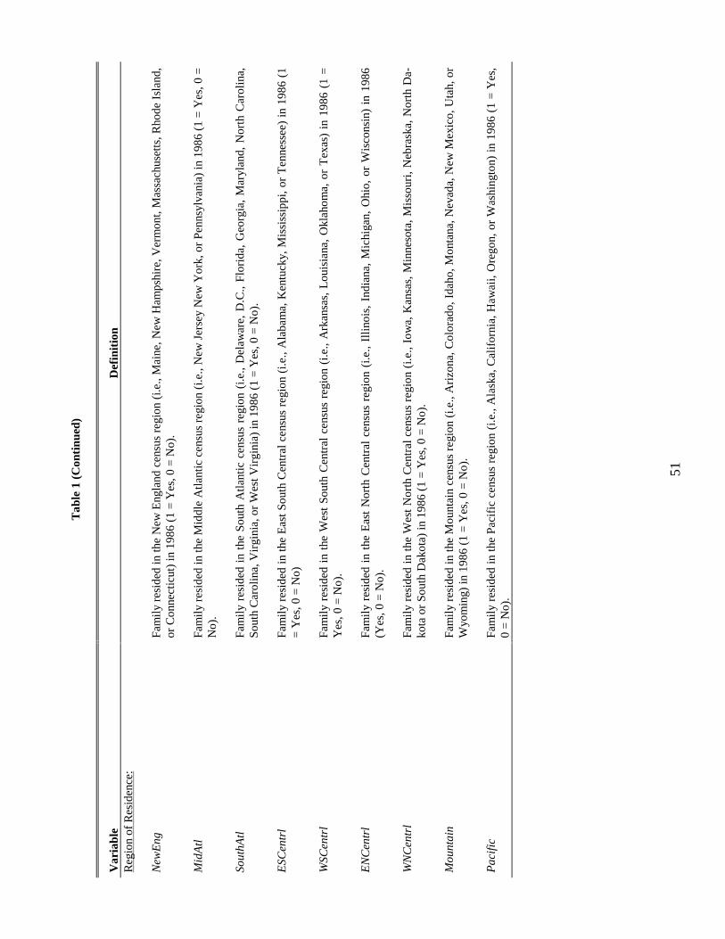
51

Tab

le 1

(C

onti

nued

)

Var

iabl

eD

efin

itio

nR

egio

n of

Res

iden

ce:

New

Eng

Fam

ily r

esid

ed in

the

New

Eng

land

cen

sus

regi

on (

i.e.,

Mai

ne, N

ew H

amps

hire

, Ver

mon

t, M

assa

chus

etts

, Rho

de I

slan

d,or

Con

nect

icut

) in

198

6 (1

= Y

es, 0

= N

o).

Mid

Atl

Fam

ily r

esid

ed in

the

Mid

dle

Atla

ntic

cen

sus

regi

on (

i.e.,

New

Jer

sey

New

Yor

k, o

r P

enns

ylva

nia)

in 1

986

(1 =

Yes

, 0 =

No)

.

Sout

hAtl

Fam

ily r

esid

ed i

n th

e So

uth

Atla

ntic

cen

sus

regi

on (

i.e.,

Del

awar

e, D

.C.,

Flor

ida,

Geo

rgia

, M

aryl

and,

Nor

th C

arol

ina,

Sout

h C

arol

ina,

Vir

gini

a, o

r W

est V

irgi

nia)

in 1

986

(1 =

Yes

, 0 =

No)

.

ESC

entr

lFa

mily

res

ided

in th

e E

ast S

outh

Cen

tral

cen

sus

regi

on (

i.e.,

Ala

bam

a, K

entu

cky,

Mis

siss

ippi

, or

Ten

ness

ee)

in 1

986

(1=

Yes

, 0 =

No)

WSC

entr

lFa

mily

res

ided

in

the

Wes

t So

uth

Cen

tral

cen

sus

regi

on (

i.e.,

Ark

ansa

s, L

ouis

iana

, O

klah

oma,

or

Tex

as)

in 1

986

(1 =

Yes

, 0 =

No)

.

EN

Cen

trl

Fam

ily

resi

ded

in t

he E

ast

Nor

th C

entr

al c

ensu

s re

gion

(i.e

., Il

lino

is,

Indi

ana,

Mic

higa

n, O

hio,

or

Wis

cons

in)

in 1

986

(Yes

, 0 =

No)

.

WN

Cen

trl

Fam

ily r

esid

ed i

n th

e W

est

Nor

th C

entr

al c

ensu

s re

gion

(i.e

., Io

wa,

Kan

sas,

Min

neso

ta, M

isso

uri,

Neb

rask

a, N

orth

Da-

kota

or

Sout

h D

akot

a) in

198

6 (1

= Y

es, 0

= N

o).

Mou

ntai

nF

amil

y re

side

d in

the

Mou

ntai

n ce

nsus

reg

ion

(i.e

., A

rizo

na, C

olor

ado,

Ida

ho, M

onta

na, N

evad

a, N

ew M

exic

o, U

tah,

or

Wyo

min

g) in

198

6 (1

= Y

es, 0

= N

o).

Pac

ific

Fam

ily r

esid

ed in

the

Pac

ific

cen

sus

regi

on (

i.e.,

Ala

ska,

Cal

ifor

nia,

Haw

aii,

Ore

gon,

or

Was

hing

ton)

in

1986

(1

= Y

es,

0 =

No)

.

52

Table 2Sample Means and Standard Deviations

(Data Source: NLS72)(Weighted)

Variable Obs. Mean Std. Dev.

UseCC 2645 0.589 0.492HrsCC 2645 16.740 19.869CCPrice 1376 1.79 2.50Work 2645 0.568 0.495InWage 1210 2.102 0.542Ratio2 2474 7.295 2.804Ratio4 2474 13.156 3.516FamEd 2474 0.383 0.486CenterEd 2474 0.590 0.492SCCSub 2474 0.036 0.055SMaxCSub 2474 0.0020 0.0032TitleXX 2474 11.494 3.718SpEarn 2395 2.341 1.873NonLbInc 2409 0.162 0.518TwoYr 2645 0.102 0.303SomeColl 2645 0.274 0.446Coll 2645 0.214 0.410MoreColl 2645 0.056 0.229Black 2645 0.098 0.297NumPre 2645 1.264 0.665NumSch 2645 0.860 0.924LivWRels 2645 0.050 0.218MomClose 2411 0.397 0.489UnempRt 2474 7.087 1.914MaxBen 2474 0.0510 0.0184BrkEven 2645 0.0685 0.0295NewEngl 2474 0.066 0.248MidAtl 2474 0.147 0.355SouthAtl 2474 0.150 0.357ESCentrl 2474 0.062 0.242WSCentrl 2474 0.102 0.303ENCentrl 2474 0.193 0.395WNCentrl 2474 0.101 0.302Mountain 2474 0.066 0.249Pacific 2474 0.112 0.315

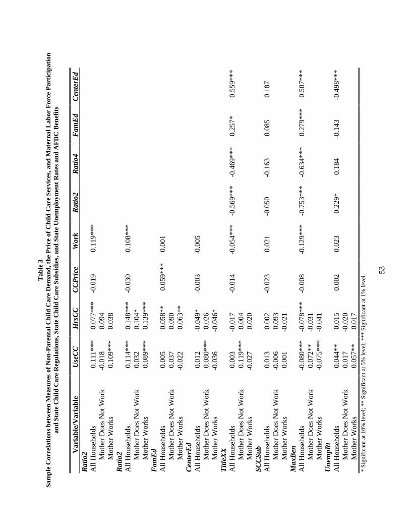
53

Tab

le 3

Sam

ple

Cor

rela

tion

s be

twee

n M

easu

res

of N

on-P

aren

tal C

hild

Car

e D

eman

d, t

he P

rice

of

Chi

ld C

are

Serv

ices

, and

Mat

erna

l Lab

or F

orce

Par

tici

pati

onan

d St

ate

Chi

ld C

are

Reg

ulat

ions

, Sta

te C

hild

Car

e Su

bsid

ies,

and

Sta

te U

nem

ploy

men

t R

ates

and

AF

DC

Ben

efit

s

Var

iabl

e/V

aria

ble

Use

CC

Hrs

CC

CC

Pri

ceW

ork

Rat

io2

Rat

io4

Fam

Ed

Cen

terE

dR

atio

2A

ll H

ouse

hold

s0.

111*

**0.

077*

**-0

.019

0.11

9***

Mot

her

Doe

s N

ot W

ork

-0.0

180.

094

Mot

her

Wor

ks0.

109*

**0.

038

Rat

io2

All

Hou

seho

lds

0.11

4***

0.14

8***

-0.0

300.

108*

**M

othe

r D

oes

Not

Wor

k0.

032

0.10

4*M

othe

r W

orks

0.08

9***

0.13

9***

Fam

Ed

All

Hou

seho

lds

0.00

50.

058*

*0.

059*

**0.

001

Mot

her

Doe

s N

ot W

ork

0.03

70.

090

Mot

her

Wor

ks-0

.022

0.06

3**

Cen

terE

dA

ll H

ouse

hold

s0.

012

-0.0

49*

-0.0

03-0

.005

Mot

her

Doe

s N

ot W

ork

0.08

0***

0.02

6M

othe

r W

orks

-0.0

36-0

.046

*T

itleX

XA

ll H

ouse

hold

s0.

003

-0.0

17-0

.014

-0.0

54**

*-0

.569

***

-0.4

69**

*0.

257*

0.55

9***

Mot

her

Doe

s N

ot W

ork

0.11

9***

0.00

4M

othe

r W

orks

-0.0

270.

020

SCC

Sub

All

Hou

seho

lds

0.01

30.

002

-0.0

230.

021

-0.0

50-0

.163

0.08

50.

187

Mot

her

Doe

s N

ot W

ork

-0.0

060.

093

Mot

her

Wor

ks0.

001

-0.0

21M

axB

enA

ll H

ouse

hold

s-0

.080

***

-0.0

78**

*-0

.008

-0.1

29**

*-0

.753

***

-0.6

34**

*0.

279*

**0.

507*

**M

othe

r D

oes

Not

Wor

k0.

072*

*-0

.031

Mot

her

Wor

ks-0

.075

***

-0.0

41U

nem

pRt

All

Hou

seho

lds

0.04

4**

0.01

50.

002

0.02

30.

229*

0.18

4-0

.143

-0.4

98**

*M

othe

r D

oes

Not

Wor

k0.

017

-0.0

20M

othe

r W

orks

0.05

7**

0.01

7*

Sig

nifi

cant

at 1

0% le

vel;

**

Sig

nifi

cant

at 5

% le

vel;

***

Sig

nifi

cant

at 1

% le

vel.

54

Tab

le 4

Est

imat

ed E

last

icit

ies

for

Var

iabl

es in

Con

diti

onal

Uti

lizat

ion

of N

on-P

aren

tal C

hild

Car

e E

quat

ions

, Con

diti

onal

Tot

al W

eekl

y H

ours

of

Chi

ld C

are

Equ

atio

ns,

Mot

her’

s L

abor

For

ce P

arti

cipa

tion

Equ

atio

n, M

othe

r’s

(Log

) W

age

Equ

atio

n an

d H

ourl

y P

rice

of

Chi

ld C

are

Equ

atio

na

Non

-Par

enta

l Chi

ld C

are

Util

izat

ion:

Wee

kly

Hou

rs o

f C

are:

Var

iabl

eW

orki

ngM

othe

rsN

on-W

orki

ngM

othe

rsW

orki

ngM

othe

rsN

on-W

orki

ngM

othe

rsL

abor

For

ceP

arti

cipa

tion

Chi

ld C

are

Pri

ceIn

Wag

eR

atio

2.2

06-.

003*

**-.

028*

**.4

52**

.109

***

.062

*R

atio

4-1

.351

***

-.06

6***

.208

-.83

1-.

995*

**-.

793*

**F

amE

db.3

11**

-.30

7***

.011

.133

.198

**.1

88**

*C

ente

rEdb

-.09

0**

.459

***

.024

-.18

8.0

17-.

018

Tit

leX

X-.

063*

**SC

CSu

b.0

14**

*.0

30**

*.0

01.0

63**

*SM

axC

Sub

.002

-.03

4***

-.00

0-.

055*

**C

CP

rice

-1.7

58**

*-1

.031

*.0

89-1

.413

-1.2

61**

*W

age

3.55

5**

2.15

92.

956*

**Sp

Ear

n-.

024

-.99

8**

-.84

3***

-2.3

92**

*-1

.828

***

Non

LbI

nc.0

15.2

31**

*.0

97**

*.3

72**

*-.

088*

**M

axB

en.5

23**

*-.

000

.217

-.21

1***

.020

Brk

Eve

n.1

86**

*-.

000

-.05

3-.

063*

**U

nem

pRt

-.27

9**

-.07

6***

Tw

oYrb

-.51

7**

.134

**-.

198

.073

-.21

7.0

68**

*So

meC

ollb

-.86

5**

.240

***

-.18

8-.

154

-.46

3*.1

21**

*C

ollb

-1.2

92**

.533

***

-.27

3.0

68-.

882*

*.1

85**

*M

oreC

ollb

-1.8

98**

1.07

0***

-.25

4.3

91-1

.386

**.2

97**

*N

umP

re.0

38**

*.0

91*

.076

***

-.32

1***

-.22

3***

Num

Sch

-.06

3***

-.20

5***

-.02

6**

-.05

6-.

070*

**L

ivW

Rel

sb.0

81**

*-.

265*

**.1

35**

*-.

205

.234

***

Mom

Clo

seb

.030

***

-.02

3-.

052*

**.0

86**

.136

***

Bla

ckb

.553

**.7

99**

*.1

34.7

84**

*.4

33**

*.0

89**

*-.

051*

**Sa

mpl

e Si

ze12

3579

298

819

320

2212

9511

49*

Sig

nifi

cant

at 1

0% le

vel;

**

Sig

nifi

cant

at 5

% le

vel;

***

Sig

nifi

cant

at 1

% le

vel.

a All

ela

stic

itie

s ar

e ev

alua

ted

at m

eans

for

rel

evan

t sam

ple

and

wor

king

or

non-

wor

king

sub

sam

ples

.b T

he c

alcu

lati

ons

for

effe

cts

wit

h re

spec

t to

dum

my

vari

able

s gi

ve th

e pe

rcen

tage

cha

nge

in th

e ou

tcom

e va

riab

le (

or p

roba

bili

ty)

due

to a

cha

nge

in th

e du

mm

y va

riab

le f

rom

0 to

1.

55

Table 5Total Estimated Effects (Expressed as Elasticities) of Regulation and Subsidy Variables on Utilization

of Non-Parental Care and the Mother’s Labor Force Participation Decisionsa

Variable OutcomeUtilization of Non-Parental Care for Households with:

Non-WorkingMothers

WorkingMothers All

Ratio2 -.064 .093 .077Ratio4 .726 .077 .205FamEda -.501 -.019 -.132CenterEda .477 -.058 .065SCCSub .014 .047SMaxCSub .002 -.029TitleXX .067 .109 .145Maxben .501 -.034 -.073NonLbInc .231 .015 .002CCPrice -1.031 -1.758 -2.331Wage 3.555 4.508

Hours of Non-Parental Care Used by Households with:

Non-WorkingMothers

WorkingMothers All

Ratio2 .370 -.022 .102Ratio4 .268 .133 .154FamEda -.133 .028 -.029CenterEda -.162 .022 -.020SCCSub .001 .030 .034SMaxCSub -.000 -.034 -.034TitleXX .091 -.006 .040Maxben .217 .002 -.005NonLbInc .372 .097 .112CCPrice -1.413 .089 -.647Wage 2.159 1.113

Mother’s LaborForce Participa-

tion Rate:Ratio2 0.030Ratio4 .005FamEda -.039CenterEda .040SCCSub .063SMaxCSub -.055TitleXX .054Maxben -.237NonLbInc -.088CCPrice -1.261Wage 2.956aSee notes to Table 4.

56

AppendixThe Data Used from the Fifth Follow-Up of the

National Longitudinal Study of the High School Class of 1972 (NLS72)

The Sample Used:

In this Appendix we provide a brief description of the NLS72 sample, the content of the

Fifth Follow-Up survey and the way we selected the analysis sample for this study. Respondents

in the NLS72 were high school seniors in U.S. schools during the 1971-1972 school year. The sam-

ple interviewed in the Fifth Follow-Up survey was generated by a two-stage sampling procedure.29

In the first stage—which generated the original sample of high school seniors—students were ran-

domly selected from schools which themselves were randomly drawn from each of 608 strata based

on type of school (public versus private), geographic region, proportion of minority students, in-

come level of community, and other criteria. Generally, 18 students were chosen at random from

each of the selected schools, but students in low-income areas and schools with a high proportion of

minorities were oversampled. The original sample consisted of 22,652 respondents, with approxi-

mately equal numbers of males and females.

At the time of the Fifth Follow-Up survey, a subset of the original members was selected for

re-interview. To be considered for the re-interview, members of the original sample had to have

participated in at least one of the earlier waves of the NLS72. Among these respondents, the subset

was selected probabilistically, with retention probabilities depending on: (i) their base-year selec-

tion probabilities; (ii) whether they had completed an interview during the fourth Follow-Up; (iii)

their ethnicity (Hispanics were retained at a higher rate); (iv) their educational status (respondents

with four-year college degrees or who had completed two years or less of college at the time of the

fourth Follow-Up were oversampled); (v) their marital status (divorced, widowed, separated and

never-married respondents were oversampled); and (vi) whether they were identified in the fourth

29 The following discussion draws heavily from Tourangeau, et al. [1987].

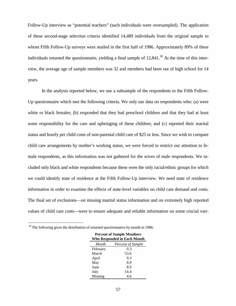
57

Follow-Up interview as “potential teachers” (such individuals were oversampled). The application

of these second-stage selection criteria identified 14,489 individuals from the original sample to

whom Fifth Follow-Up surveys were mailed in the first half of 1986. Approximately 89% of these

individuals returned the questionnaire, yielding a final sample of 12,841.30 At the time of this inter-

view, the average age of sample members was 32 and members had been out of high school for 14

years.

In the analysis reported below, we use a subsample of the respondents to the Fifth Follow-

Up questionnaire which met the following criteria. We only use data on respondents who: (a) were

white or black females; (b) responded that they had preschool children and that they had at least

some responsibility for the care and upbringing of these children; and (c) reported their marital

status and hourly per child costs of non-parental child care of $25 or less. Since we wish to compare

child care arrangements by mother’s working status, we were forced to restrict our attention to fe-

male respondents, as this information was not gathered for the wives of male respondents. We in-

cluded only black and white respondents because these were the only racial/ethnic groups for which

we could identify state of residence at the Fifth Follow-Up interview. We need state of residence

information in order to examine the effects of state-level variables on child care demand and costs.

The final set of exclusions—on missing marital status information and on extremely high reported

values of child care costs—were to ensure adequate and reliable information on some crucial vari-

30 The following gives the distribution of returned questionnaires by month in 1986:

Percent of Sample MembersWho Responded in Each Month

Month Percent of SampleFebruary 0.3March 53.6April 9.3May 8.9June 8.9July 14.4Missing 4.6

58

ables. Our final sample includes 2,645 respondents.

As noted in the text, this is not a random sample of mother-present households with pre-

school age children. There are several dimensions in which it is non-representative of this popula-

tion. First, the NLS72 only sampled individuals who were seniors in the 1971-1972 school-year.

Second, the women in our sample, who were around 31 years of age at the time of the survey, are

older than the average age of mothers with preschool age children in the U.S. In Hotz and Kilburn

[1992], we conducted a detailed comparison of the characteristics with our sample of women from

the NLS72 with a representative sample of households with preschoolers from the 1986 Current

Population Survey (CPS). Despite the discrepancies between the two populations noted above,

based on a comparison of a range of demographic characteristics and measures of economic status,

we find that our sample from the NLS72 looks a good deal like the population of households with

preschool age children. This is especially true when comparing our sample with U.S. households

with mothers between the ages of 30 and 35. Thus, while appropriately cautious about the gener-

alizability of our findings, we anticipate that our results are applicable to households in which the

mothers fall within the age cohort covered by the NLS72, and may apply to the broader population

of those households with young children present.

The Variables Used:

The respondents to Fifth Follow-Up survey were asked a range of questions about their

child care arrangements and expenses as well as about their family income and the respondent’s la-

bor supply. In addition, using information on the state of residence at the 1986 interview, we sup-

plemented the survey data with state-level variables, including measures of the prevailing child care

regulations. Here we briefly describe the data available and the variables we constructed.

The Fifth Follow-Up questionnaire asked child care information in two modules. The first

module covered child care arrangements for preschool age children, while the second covered ar-

59

rangements for school-age children. In this paper, we focus on the information in the first module.31

Respondents were asked to “describe the usual child care arrangements” for their preschool chil-

dren. They were asked to “circle all that apply,” and indicate the average numbers of hours per

week for each one circled for the following list of particular child care arrangements:

(a) Not applicable; I have no preschool age children(b) Mother or father cares for child at home(c) In child’s home by relative(d) In child’s home by non-relative(e) In relative’s home(f) In non-relative’s home(g) Private day care center or nursery school, other than kindergarten(h) Public day care center or nursery school, other than kindergarten(i) Child cares for self (without supervision)(j) Mother or father cares for child at work(k) Employer-provided day care(l) Other (specify)(m) Don’t know

They were also asked: “Thinking back over the last six months, how much money did you usually

spend on child care for all your preschool children during an average month?”

From these responses, we constructed several variables measuring non-parental child care

utilization and costs. The definitions of these and the other variables used in the paper are found in

Table 1 and their sample means and standard deviations are reported in Table 2. The variable

UseCC is a dichotomous variable which measures whether the respondent used only parental child

care (UseCC = 0) or if she used some non-parental care (UseCC = 1). Since the questionnaire only

includes the response “mother or father cares for child at home (or work),” we are not able to de-

termine whether parental care was only provided by the mother or by both parents.

To measure the intensity of non-parental child care utilization, we constructed the variable,

HrsCC, measuring the average hours per week (and per child) of care used. Finally, using the re-

sponses on typical child care expenditures, we constructed the variable CCPrice, which gives the

31 The questionnaire did not specify the ages of these two groups of children, but we found that the preschool age chil-

60

average cost per hour (per child) of non-parental child care. As we discuss in the text, the limited

information collected on the child care in the 1986 wave prevents us from conducting an analysis of

the particular mode of care parents use and the average prices paid for specific modes.

The other crucial dimension for our analysis is the labor force status of the mother. As noted

in the Introduction, most existing surveys only ask working mothers or mothers in school or in

training programs about their child care arrangements. In order to classify our respondents accord-

ing to these work and training distinctions, we used their responses to a modified version of the

CPS labor-force-activity question asked for the reference period of the first week of February 1986.

We classified a woman in one of two categories: (a) “Working” if she reported that she was “work-

ing for pay at a full-time or part-time job” or on active duty in the military; (b) “Not Working,” if

she was not working or was not working but was taking technical, college, or graduate courses or

was in an apprentice program. We find that 57% of the mothers in the sample were working.32 For

respondents working in February, we constructed a measure of their hourly wage, labeled Wage,

using her “highest current or ending hourly wage rate (before deductions)” reported for any jobs

held during the first week of February 1986.

The other variables defined in Table 1—in particular, the measures of state child care regu-

lations, child care subsidies, and tax credits—are described in section 2.3 of the paper.

dren were generally less than six years old, and that the school-age children were generally six years old and above.

32 Inadvertently, we did not include those households with mothers who reported that they had a job but were temporar-ily not at work in the “Working” category. Such women would be classified as working by the standard CPS labor forcestatus classification scheme and would be asked the child care questions in most of the existing surveys. We have inves-tigated the sensitivity of our analysis to this misclassification and found that it had not discernible impact on the resultsreported here.

61

Table AMaximum Likelihood Parameter Estimates for Conditional Utilization of Non-Parental Care Decisions, Con-ditional Weekly Hours of Child Care Used per Child, Hourly Price of Child Care Equation, Mother’s Labor

Force Participation and (Log) Wage Equations[Data Source: NLS72, 1986 Wave]

Child Care Utilization: Weekly Hours of Child Care:Variable Working

MothersNon-Working

MothersWorkingMothers

Non-WorkingMothers

Labor ForceParticipation

Ratio2 .0736* -.1157*** -1.6466*** -3.4151** -.0694***(.0409) (.0380) (.3266) (1.3723) (.0196)

Ratio22 .0014 .0083*** .0992*** .3377*** .0062***(.0017) (.0024) (.0192) (.0870) (.0011)

Ratio4 -.4583*** -.2512*** .1838 .1857 -.0887(.1445) (.0327) (.8898) (2.4041) (.2294)

Ratio42 .0040*** .0097*** .0110 -.0520 -.0008(.0009) (.0010) (.0101) (.0711) (.0005)

FamEd 1.0840** -.2447*** .2921 2.3853 .2857**(.4220) (.0714) (2.3419) (4.9947) (.1200)

CenterEd -.3134** .3655*** .7533 -3.4261 .0248(.1531) (.0377) (.6774) (2.7871) (.0488)

SCCSub 1.3227*** 24.1629*** 2.5111***(.5092) (5.7084) (.2305)

SMaxCSub .0415 -.5318*** -.4293***(.0951) (.1063) (.0436)

CCPrice -3.5170*** -.4725* 1.7351 -14.5498 -1.0465***(1.3072) (.2891) (7.4622) (15.8332) (.3655)

lnWage 12.3611** 18.8694 4.1842***(5.0756) (25.4895) (1.5001)

SpEarn -.0040 -.0293** -1.2547*** -1.5941*** -.1128***(.0126) (.0117) (.1436) (.3173) (.0030)

NonLbInc .0345 .1020*** 1.9852*** 2.7245*** -.0789***(.0248) (.0161) (.3198) (.8341) (.0114)

MaxBen .0775*** .8058 -.0599***(.0165) (.7206) (.0085)

BrkEven .0179*** -.1111 -.0111***(.0038) (.1564) (.0022)

TwoYr -1.8025** .1068** -6.0086 1.3416 -.3138(.7372) (.0453) (3.6666) (1.2133) (.2206)

SomeColl -3.0197** .1910*** -5.6403 -2.7338 -.6698*(1.2896) (.0450) (6.2871) (1.7497) (.3821)

Coll -4.5068** .4252*** -8.1971 1.3437 -1.2748**(1.9679) (.0435) (9.5087) (3.1020) (.5826)

MoreColl -6.6210** .8528*** -7.5058 7.2460 -2.0040**(3.1673) (.0741) (14.9604) (6.0167) (.9360)

NumPre .1142*** .0523* 1.9694*** -4.0425*** -.2555***(.0272) (.0282) (.3373) (.7422) (.0078)

NumSch -.2682*** -.1779*** -1.0606** -1.3720 -.1180***(.0142) (.0160) (.4721) (1.4087) (.0055)

MomClose .1054*** -.0183 -1.5992*** 1.5454** .1961***(.0249) (.0298) (.3501) (.7293) (.0109)

LivWRels .2844*** -.2116*** 4.1366*** -3.7437 .3378***(.0476) (.0686) (.7832) (3.9623) (.0296)

62

Table A (Continued)

Child Care Utilization: Weekly Hours of Child Care:Variable Working

MothersNon-Working

MothersWorkingMothers

Non-WorkingMothers

Labor ForceParticipation

Black 1.9296** .6366*** 4.0416 14.0861*** .6265***(.7578) (.0625) (3.9717) (4.9324) (.2219)

MidAtl -.3533 -.5490*** 4.0232** -1.9927 -.8254***(.4982) (.1250) (1.8391) (6.4511) (.1451)

SouthAtl 1.4925*** -.4926*** 3.6372 3.0652 .0531(.4547) (.0948) (2.8002) (7.0182) (.1380)

ESCentrl 4.9037*** .4960** 5.9276 31.2201 .9860**(1.5134) (.2070) (9.4667) (19.3153) (.4348)

WSCentrl 1.6191*** -.2279** 5.7080* 10.7923 -.1190(.5206) (.1131) (2.9547) (9.9700) (.1576)

ENCentrl .0927 .0547 4.3009*** 5.4303** -.4512***(.3968) (.1009) (1.1652) (2.5648) (.1200)

WNCentrl -.8849 -.6621*** 8.4985*** -1.6369 -.5414***(.6778) (.1606) (2.6576) (9.7229) (.1959)

Mountain 1.2184** .7355*** .7912 24.6512** .0581(.5467) (.0982) (2.4752) (10.0910) (.1662)

Pacific -1.2950 .1136 9.2779** 3.0095 -1.1072***(.8357) (.1186) (3.6610) (4.0328) (.2377)

Constant 12.4313* 1.3198** -7.9614 85.5002 -3.4432(6.7486) (.6351) (28.7301) (52.3698) (2.0977)

σ* 15.3760*** 12.9984***(.0558) ( .1874)

63

Table A (Continued)

Equation Error Correlations:

VariableChild Care

Price EquationlnWage

Equation Correlation EstimateRatio2 .0148*

ε νρ .0075(.0086) (1.1690)

Ratio4 -.1050***ε νρ .0053

(.0078) (4.4891)FamEd .3273***

ε ερ -.0110(.0373) (1.0021)

CenterEd -.0317ε ερ -.0010

(.0380) (.9241)TitleXX -.0095***

ν ερ -.0021(.0033) (.7370)

UnempRt -.0686*** -.0222***ν ηρ -.0121

(.0139) (.0029) (1.5964)MaxBen .0695

ε ηρ -.0924(.0430) (.1464)

TwoYr .1414***ε ηρ -.0924

(.0090) (.1464)SomeColl .2532***

ν ηρ -.1640***(.0064) (.0376)

Coll .3865***ν ηρ -.0991

(.0085) (.1465)MoreColl .6214***

ε ηρ .0890(.0138) (.0897)

Black .1543*** -.1068***ε ηρ .1943***

(.0464) (.0098) (.0521)MidAtl -.2490*** .0057

ν ηρ .0221(.0745) (.0139) (.0510)

SouthAtl .3587*** .0335***ε ηρ .0278

(.0703) (.0129) (.1059)ESCentrl 1.2222*** .0304

η ηρ .1137**(.1098) (.0250) (.0522)

WSCentrl .6570*** .1119***(.1006) (.0227)

ENCentrl -.0196 .0477***(.0850) (.0173)

WNCentrl -.4899*** -.0189(.0960) (.0134)

Mountain .5304*** .0805***(.0835) (.0209)

Pacific -.1418 .1270***(.0872) (.0171)

Constant 3.3614*** 2.0066***(.1113) (.0167)

σ* 2.4671*** .5055***(.0074) (.0011)

Log-Like. -62518.75

* Signif’icant at 10% level; ** Significant at 5% level; *** Significant at 1% level.