regularization of inverse problems - unibo.it · regularized solutions of nonlinear ill-posed...
TRANSCRIPT

Regularization of Inverse Problems
Otmar Scherzer
Computational Science Center, University Vienna, Austria&
Radon Institute of Computational and Applied Mathematics (RICAM), Linz, Austria
Otmar Scherzer (CSC & RICAM) Regularization of Inverse Problems June 7, 2018 1 / 70
Inverse Problems
desire to calculate or estimatecausal factors
from a set of observations
Otmar Scherzer (CSC & RICAM) Regularization of Inverse Problems June 7, 2018 2 / 70

Inverse Problems are often Ill-Posed
Operator equation:Lu = y
Setting:
Available data y δ of y are noisy
Focus: L is a linear operator
Ill-posed: Let u† be a solution:
y δ → y 6⇒ uδ → u†
A. N. TikhonovOn the stability of inverse problemsDoklady Akademii Nauk SSSR 39. 1943
Otmar Scherzer (CSC & RICAM) Regularization of Inverse Problems June 7, 2018 3 / 70

Examples of Ill–Posed Problems: L=
1 Identity operator: Measurements of noisy data.Applications: A.e.
2 X -Ray transform: Measurements of averagesover lines. Application: ComputerizedTomography (CT)
3 Radon transform: Measurements of averagesover hyperplanes. Application: Cryo-EM
4 Spherical Radon transform: Measurements ofaverages over spheres. Application:Photoacoustic Imaging
5 Circular Radon transform: Measurements ofaverages over circles. Applications: GroundPenetrating Radar and Photoacoustics
Otmar Scherzer (CSC & RICAM) Regularization of Inverse Problems June 7, 2018 4 / 70

An Application
GPR: Location of avalanche victims
Project with Wintertechnik AG and Alps
Otmar Scherzer (CSC & RICAM) Regularization of Inverse Problems June 7, 2018 5 / 70

Various PhilosophiesContinuous approach: L : H1 → H2. Hi infinitedimensional spaces
Semi-continuous approach: L : H → Rn. Hinfinite dimensional space, finitely manymeasurements
Discrete Setting: L : Rm → Rn. Large scaleinverse problems
Bayesian approach:L : Rm → Rn. Stochasticinverse problems
A. N. TikhonovSolution of incorrectly formulated problems and theregularization methodsSoviet Mathematics. Doklady 4. 1963
H. Engl, M. Hanke, and A. NeubauerRegularization of inverse problemsKluwer Academic Publishers Group, 1996
M. Unser, J. Fageot, and J. P. WardSplines are universal solutions of linear inverseproblems with generalized TV regularizationSIAM Review 59.4. 2017
C. R. VogelComputational Methods for Inverse ProblemsSIAM, 2002
M. Hanke and P. C. HansenRegularization methods for large-scale problemsSurveys on Mathematics for Industry 3.4. 1994
J. Kaipio and E. SomersaloStatistical and Computational Inverse ProblemsSpringer Verlag, 2005
Otmar Scherzer (CSC & RICAM) Regularization of Inverse Problems June 7, 2018 6 / 70

Deterministic Setting
From Continuous approach: L : H1 → H2. Hi infinite dimensional spaces⇒
Semi-Continuous approach: P L with P[f ] = (f (xi ))i=1,...,n
Discrete approach: P L Q with Q[(ci )i=1,...,m](x) =∑m
i=1 ciφ(x).(φi ) family of test functions.
A. Neubauer and O. ScherzerFinite-dimensional approximation of Tikhonovregularized solutions of nonlinear ill-posed problemsNumer. Funct. Anal. Optim. 11.1-2. 1990
C. Poschl, E. Resmerita, and O. ScherzerDiscretization of variational regularization inBanach spacesInverse Probl. 26.10. 2010
Otmar Scherzer (CSC & RICAM) Regularization of Inverse Problems June 7, 2018 7 / 70

Various Methods to Solve
Backprojection formulas
Iterative Methods for linear and nonlinear inverse problems
Flow methods: Showalter’s methods and Inverse scale space methods
Variational methods: Tikhonov type regularization.
...
J. RadonUber die Bestimmung von Funktionen durch ihreIntegralwerte langs gewisser MannigfaltigkeitenBerichte uber die Verhandlungen derKoniglich-Sachsischen Gesellschaft derWissenschaften zu Leipzig,Mathematisch-Physische Klasse 69. 1917
M. Hanke and P. C. HansenRegularization methods for large-scale problemsSurveys on Mathematics for Industry 3.4. 1994
B. Kaltenbacher, A. Neubauer, and O. ScherzerIterative regularization methods for nonlinearill-posed problemsWalter de Gruyter, 2008
O. Scherzer and C. W. Groetsch (2001). “InverseScale Space Theory for Inverse Problems”. In:Scale-Space and Morphology in Computer Vision.Ed. by M. Kerckhove. Vol. 2106. Lecture Notes inComputer Science. Vancouver, Canada: Springer,pp. 317–325. isbn: 978-3-540-42317-1. doi:10.1007/3-540-47778-0_29. url:http://dx.doi.org/10.1007/3-540-47778-0_29
H. Engl, M. Hanke, and A. NeubauerRegularization of inverse problemsKluwer Academic Publishers Group, 1996
O. Scherzer, M. Grasmair, H. Grossauer,M. Haltmeier, and F. LenzenVariational methods in imagingSpringer, 2009
Otmar Scherzer (CSC & RICAM) Regularization of Inverse Problems June 7, 2018 8 / 70

Outline
2 Numerical Differentiation
1 Variational Methods
3 General Regularization
4 Sparsity and `1-Regularization
5 TV-Regularization
6 Regularization of High-Dimensional Data
Otmar Scherzer (CSC & RICAM) Regularization of Inverse Problems June 7, 2018 9 / 70

Numerical Differentiation
Numerical Differentiation as an Inverse Problem
y = y(x) is a smooth function on 0 ≤ x ≤ 1
Given: Noisy samples y δi of y(xi ) on a uniform grid
∆ = 0 = x0 < x1 < · · · < xn = 1, h = xi+1 − xi
satisfying ∣∣∣y δi − y(xi )∣∣∣ ≤ δ
Boundary data are known exactly: y δ0 = y(0) and y δn = y(1)
Goal: Find a smooth approximation u′ of y ′
M. Hanke and O. ScherzerInverse problems light: numerical differentiationAmer. Math. Monthly 108.6. 2001
M. Hanke and O. ScherzerError analysis of an equation error method for theidentification of the diffusion coefficient in aquasi-linear parabolic differential equationSIAM J. Appl. Math. 59.3. 1999
Otmar Scherzer (CSC & RICAM) Regularization of Inverse Problems June 7, 2018 10 / 70

Numerical Differentiation
Strategy I: Constrained Minimization
Approach: Continuous to discrete
1 ‖u′′‖2L2 =
∫ 10 (u′′)2 dx → min among smooth functions u satisfying
I u(0) = y(0), u(1) = y(1),I Constraint:
1
n − 1
n−1∑i=1
(yδi − u(xi )
)2 ≤ δ2
2 Minimizer u∗: u′∗ ≈ y ′
Otmar Scherzer (CSC & RICAM) Regularization of Inverse Problems June 7, 2018 11 / 70

Numerical Differentiation
Strategy II: Tikhonov Regularization
1 Let α > 0. Minimization among smooth functions u satisfyingu(0) = y(0), u(1) = y(1), of
uδα = argminΦ[u], Φ[u] =1
n − 1
n−1∑i=1
(y δi − u(xi )
)2+ α
∥∥u′′∥∥2
L2
2 uδα′ ≈ y ′
Otmar Scherzer (CSC & RICAM) Regularization of Inverse Problems June 7, 2018 12 / 70

Numerical Differentiation
Strategy II: Tikhonov Regularization + DiscrepancyPrinciple
Theorem
If α is selected according to the discrepancy principle
1
n − 1
n−1∑i=1
(y δi − uδα(xi )
)2= δ2
Then Strategy I and II are equivalent: uδα = u∗
V. A. MorozovMethods for Solving Incorrectly Posed ProblemsSpringer, 1984
Otmar Scherzer (CSC & RICAM) Regularization of Inverse Problems June 7, 2018 13 / 70

Numerical Differentiation
Analysis of Constrained Optimization
Let
1 y ′′ ∈ L2(0, 1) (assumption on the data to be reconstructed) and
2 u∗ be the minimizer of Strategy II
Then ∥∥u′∗ − y ′∥∥L2 ≤
√8(h∥∥y ′′∥∥
L2︸ ︷︷ ︸approx. error
+√δ ‖y ′′‖L2︸ ︷︷ ︸
noise influence
)
I. J. SchoenbergSpline interpolation and the higher derivativesProceedings of the National Academy of Sciencesof the USA 51.1. 1964
M. UnserSplines: a perfect fit for signal and imageprocessingIEEE Signal Processing Magazine 16.6. 1999
Otmar Scherzer (CSC & RICAM) Regularization of Inverse Problems June 7, 2018 14 / 70

Numerical Differentiation
Textbook Example: Numerical Differentiation
Let y ∈ C 2[0, 1], then∣∣∣∣∣y δi+1 − y δih
− y ′(x)
∣∣∣∣∣ ≤ O( h︸︷︷︸approx. error
+ δ/h︸︷︷︸noise error
), xi ≤ x ≤ xi+1
Figure: h → h + δ/h (numerical differentiation) and
h → h +√δ (Tikhonov regularization) for fixed δ
y ′′ ∈ L2: h → h + δ/h is minimalfor h ∼
√δ. Optimal rates for
Strategy I, II and numerical differ-entiation is O(
√δ)
The rate O(√δ) does not hold if
y ′′ /∈ L2(0, 1)
Otmar Scherzer (CSC & RICAM) Regularization of Inverse Problems June 7, 2018 15 / 70

Numerical Differentiation
Properties of u∗
Theorem
a solution u∗ of Strategy I exists
u∗ is a natural cubic spline, i.e.,I a function that is twice continuously differentiable over [0, 1] withI u′′∗ (0) = u′′∗ (1) = 0, and coincides on each subinterval [xi−1, xi ] of ∆
with some cubic polynomial
Generalizations of the ideas to non-quadratic regularization and general inverse problemsin Adcock and A. C. Hansen 2015; Unser, Fageot, and Ward 2017
B. Adcock and A. C. HansenGeneralized sampling and the stable and accuratereconstruction of piecewise analytic functions fromtheir Fourier coefficientsMath. Comp. 84.291. 2015
M. Unser, J. Fageot, and J. P. WardSplines are universal solutions of linear inverseproblems with generalized TV regularizationSIAM Review 59.4. 2017
Otmar Scherzer (CSC & RICAM) Regularization of Inverse Problems June 7, 2018 16 / 70

General Regularization
General Variational Methods: Setting
General: Numerical differentiation:
H1 and H2 are Hilbert spaces H1 = W 20 (0, 1) = w :
w ,w ′ ∈ L2(0, 1) andH2 = Rn−1
L : H1 → H2 linear andbounded
L : W 20 (0, 1)→ Rn−1,
u 7→ (u(xi ))1≤i≤n−1
ρ : H2 × H2 → R+ similarityfunctional
ρ(ξ, ν) = 1n−1
∑n−1i=1 (ξi − νi )2
R : H1 → R+ an energyfunctional
R[u] =∫ 1
0 (u′′)2 dx
δ: estimate for the amount ofnoise
1n−1
∑n−1i=1 (yi − y δi )2 ≤ δ2.
Otmar Scherzer (CSC & RICAM) Regularization of Inverse Problems June 7, 2018 17 / 70

General Regularization
Three Kind of Variational Methods (τ ≥ 1)
1 Residual method:
uδα = argminR(u)→ min subject to ρ(Lu, y δ) ≤ τδ
2 Tikhonov regularization with discrepancy principle:
uδα := argminρ2(Lu, y δ) + αR(u)
,
where α > 0 is chosen according to Morozov’s discrepancy principle,i.e., the minimizer uδα of the Tikhonov functional satisfies
ρ(Luδα, yδ) = τδ
3 Tikhonov regularization with a–priori parameter choice: α = α(δ)
Otmar Scherzer (CSC & RICAM) Regularization of Inverse Problems June 7, 2018 18 / 70

General Regularization
Relation between Methods
E.g. R convex and ρ2(a, b) = ‖a− b‖2
Residual Method ≡ Tikhonov with discrepancy principle
Note, this was exactly the situation in the spline example!
V. K. Ivanov, V. V. Vasin, and V. P. TananaTheory of linear ill-posed problems and itsapplicationsVSP, 2002
Otmar Scherzer (CSC & RICAM) Regularization of Inverse Problems June 7, 2018 19 / 70
General Regularization
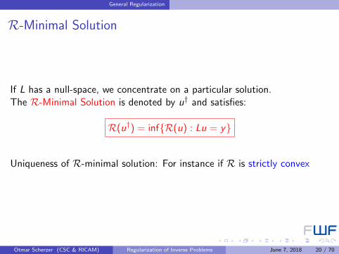
R-Minimal Solution
If L has a null-space, we concentrate on a particular solution.The R-Minimal Solution is denoted by u† and satisfies:
R(u†) = infR(u) : Lu = y
Uniqueness of R-minimal solution: For instance if R is strictly convex
Otmar Scherzer (CSC & RICAM) Regularization of Inverse Problems June 7, 2018 20 / 70

General Regularization
Regularization Method
A method is called a regularization method if the following holds:
Stability for fixed α: y δ →H2 y ⇒ uδα →H1 uα
Convergence: There exists a parameter choice α = α(δ) > 0 suchthat y δ →H2 y ⇒ uδα(δ) →H1 u†
It is an efficient regularization method if there exists a parameter choiceα = α(δ) such that
D(uδα(δ), u†) ≤ f (δ) ,
where
D is an appropriate distance measure
f rate (f → 0 for δ → 0)
Otmar Scherzer (CSC & RICAM) Regularization of Inverse Problems June 7, 2018 21 / 70

General Regularization
Importance of Topologies
It is important to specify the topology of the convergence. TypicallySobolev or Besov spaces.
Example
Differentiation is well-posed from W 10 (0, 1) into L2(0, 1), but not from
L2(0, 1) into itself. Take
x → fn(x) :=1
nsin(2πnx)
Thenx → f ′n(x) := 2π cos(2πnx)
Note
‖fn‖2W 1
0 (0,1) =1
2
1
n2+ π → π ∼
∥∥f ′n∥∥2
L2(0,1)= π but ‖fn‖2
L2(0,1) =1
2
1
n2→ 0
Otmar Scherzer (CSC & RICAM) Regularization of Inverse Problems June 7, 2018 22 / 70
General Regularization
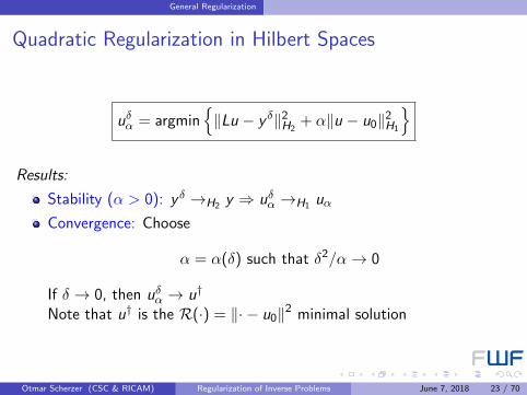
Quadratic Regularization in Hilbert Spaces
uδα = argmin‖Lu − y δ‖2
H2+ α‖u − u0‖2
H1
Results:
Stability (α > 0): y δ →H2 y ⇒ uδα →H1 uα
Convergence: Choose
α = α(δ) such that δ2/α→ 0
If δ → 0, then uδα → u†
Note that u† is the R(·) = ‖· − u0‖2 minimal solution
Otmar Scherzer (CSC & RICAM) Regularization of Inverse Problems June 7, 2018 23 / 70

General Regularization
Convergence Rates (The Simplest Case)Assumptions:
Source Condition: u† − u0 ∈ L∗η
α = α(δ) ∼ δ
Result: ∥∥∥uδα − u†∥∥∥2
= O(δ) and∥∥∥Luδα − y
∥∥∥ = O(δ)
Here L∗ is the adjoint of L, i.e.,
〈Lu, y〉 = 〈u, L∗y〉
If L ∈ Rm×n, then L∗ = LT ∈ Rn×m
If L = Radon transform, the L∗ is backprojection operator
C. W. GroetschThe Theory of Tikhonov Regularization forFredholm Equations of the First KindPitman, 1984
H. Engl, M. Hanke, and A. NeubauerRegularization of inverse problemsKluwer Academic Publishers Group, 1996
Otmar Scherzer (CSC & RICAM) Regularization of Inverse Problems June 7, 2018 24 / 70

General Regularization
Convergence Rates for the Spline Example
Recall Lu = u(0.5) (just one sampling point) and ∆ = 0, 0.5, 1.Adjoint operator of L : W 2
0 (0, 1)→ R, L∗ : R→W 20 (0, 1).
Let z be the solution of
z(IV )(x) = δ0.5(x)
satisfying z(0) = z(1) = z ′′(0) = z ′′(1) = 0 and z(0.5) = 1 andC 2-smoothness, i.e. it is a fundamental solution.
Then z is a natural cubic spline! 1
1Note that a cubic spline is infinitely often differentiable between sampling point andthe third derivative jumps. Thus fourth derivative is a δ-distribution at the samplingpoints
Otmar Scherzer (CSC & RICAM) Regularization of Inverse Problems June 7, 2018 25 / 70

General Regularization
Adjoint for the Spline Example
Let v ∈ R
〈Lu, v〉R = Luv = v
∫ 1
0u(x)δ0.5(x) dx = v
∫ 1
0u(x)z(IV )(x) dx
=
∫ 1
0u′′(x)
(vz ′′(x)
)dx = 〈u, vz〉W 2
0 (0,1)
Thus L∗v(x) = vz(x).A convergence rate O(
√δ) holds if the solution is a natural cubic spline
and u†′′ ∈ L2(0, 1) (integration by parts)
Otmar Scherzer (CSC & RICAM) Regularization of Inverse Problems June 7, 2018 26 / 70

General Regularization
Classical Convergence Rates - Spectral Decomposition
First, let L ∈ Rn×m be a matrix:
L = ΨTΛΦ with Φ ∈ Rm×m,Ψ ∈ Rn×n orthogonal
and Λ diagonal with rank ≤ min m, n.Then
L∗L = LTL = ΦTΛΨΨTΛDΦ = ΦTΛ2Φ
which rewrites to
L∗Lu =
minm,n∑n=1
λ2n〈u, φn〉φn =
∫ ∞0
λ2 〈u, φn〉δλndx︸ ︷︷ ︸=de(λ)u
Otmar Scherzer (CSC & RICAM) Regularization of Inverse Problems June 7, 2018 27 / 70

General Regularization
Classical Convergence Rates (Generalized)
Spectral Theory:
L∗L is a bounded, positive definitive, self-adjoint operator
L∗Lu =∫∞
0 λ2de(λ)u, where e(λ) denotes the spectral measure ofL∗L
If L is compact, then
L∗Lu =∞∑n=0
λ2n〈u, φn〉φn ,
where (λ2n, φn) are the spectral values of L
Otmar Scherzer (CSC & RICAM) Regularization of Inverse Problems June 7, 2018 28 / 70

General Regularization
Classical Convergence Rates
Source Condition: u† − u0 ∈ (L∗L)νη, ν ∈ (0, 1]
α = α(δ) ∼ δ2
2ν+1
Result: ∥∥∥uδα − u†∥∥∥ = O(δ
2ν2ν+1 ) and
∥∥∥Luδα − y∥∥∥ = O(δ)
Note, that for ν = 1/2
R((L∗L)1/2) = R(L∗)
C. W. Groetsch.
The Theory of Tikhonov Regularization forFredholm Equations of the First Kind.Pitman, Boston, 1984.
Otmar Scherzer (CSC & RICAM) Regularization of Inverse Problems June 7, 2018 29 / 70
General Regularization
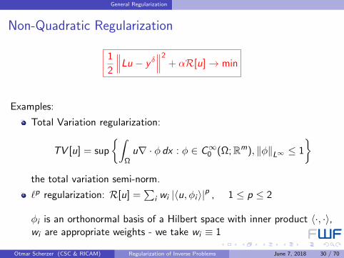
Non-Quadratic Regularization
1
2
∥∥∥Lu − y δ∥∥∥2
+ αR[u]→ min
Examples:
Total Variation regularization:
TV [u] = sup
∫Ωu∇ · φ dx : φ ∈ C∞0 (Ω;Rm), ‖φ‖L∞ ≤ 1
the total variation semi-norm.
`p regularization: R[u] =∑
i wi |〈u, φi 〉|p , 1 ≤ p ≤ 2
φi is an orthonormal basis of a Hilbert space with inner product 〈·, ·〉,wi are appropriate weights - we take wi ≡ 1
Otmar Scherzer (CSC & RICAM) Regularization of Inverse Problems June 7, 2018 30 / 70

General Regularization
Functional Analysis, Basics I
Let (un) be a sequence in a Hilbert space H, then un H u iff
〈un, φ〉H → 〈u, φ〉H ∀φ ∈ H
The set u : u ∈ L1(Ω) and TV [u] <∞
with the norm
‖u‖BV := ‖u‖L1(Ω) + TV [u]
is a Banach space and is called Space of Functions of BoundedVariation
A sequence in BV ∩ L2(Ω) is weak* convergent, un ∗ u, iff
〈un, φ〉L2(Ω) → 〈u, φ〉L2(Ω)quad∀φ ∈ L2(Ω) and TV [un]→ TV [u]
If u ∈ C 1(Ω), then TV [u] =∫
Ω |∇u| dx
L. Ambrosio, N. Fusco, and D. PallaraFunctions of bounded variation and freediscontinuity problemsOxford University Press, 2000
Otmar Scherzer (CSC & RICAM) Regularization of Inverse Problems June 7, 2018 31 / 70
General Regularization
Functional Analysis, Basics II
Let H be a Hilbert space
R : H → R ∪ +∞ is called proper if R 6=∞R is weakly lower semi-continuous if for un H u
R[u] ≤ lim infR[un]
R. T. RockafellarConvex AnalysisPrinceton University Press, 1970
Otmar Scherzer (CSC & RICAM) Regularization of Inverse Problems June 7, 2018 32 / 70

General Regularization
Non-Quadratic Regularization
Assumptions:
L is a bounded operator between Hilbert spaces H1 and H2 withclosed and convex domain D(L)
R is weakly lower semi-continuous
Results:
Stability: y δ →H2 y ⇒ uδα H2 uα and R[uδα]→ R[uα]
Convergence: y δ →H2 y and α = α(δ) such that δ2/α→ 0, then
uδα H2 u† and R[uδα]→ R[u†]
Asplund property: For quadratic regularization in H-spaces weakconvergence and convergence of the norm gives strong convergence
Otmar Scherzer (CSC & RICAM) Regularization of Inverse Problems June 7, 2018 33 / 70

General Regularization
Some Convex Analysis: The Subgradient
−1 −0.5 0.5 1
−0.5
0.5
1f (x) = |x |p1(x) = 0.5x
p2(x) = −0.25x
Illustration of the function f : (−1, 1)→ R, f (x) = |x |, and the graphs oftwo of its subgradients p1, p2 ∈ ∂f (0) = p ∈ R∗ | p(x) = cx , c ∈ [−1, 1]
Otmar Scherzer (CSC & RICAM) Regularization of Inverse Problems June 7, 2018 34 / 70

General Regularization
Some Convex Analysis: The Bregman Distance
0.5 1.5 2.5
1
2
5
6
7
8
y x
f (x)
f (y) + f ′(y)(x − y)Df (x , y)
f (x) = x2
f (y) + f ′(y)(x − y)
Illustration of the Bregman distanceDf ′(y)(x , y) = f (x)− f (y)− f ′(y)(x − y) for the function f : R→ R,f (x) = x2, between the points x = 2 and y = 1
Otmar Scherzer (CSC & RICAM) Regularization of Inverse Problems June 7, 2018 35 / 70

General Regularization
Bregman Distance
1 We consider Bregman distance for functionals
2 If R[u] = 12 ‖u − u0‖2 ⇒ ∂R[u†] = u − u†
3 and Dξ(u, v) = 12 ‖u − v‖2.
4 In general not a distance measure: It may be non-symmetric and mayvanish for non-equal elements
5 Bregman distance can be a weak measure and difficult to interpret
Otmar Scherzer (CSC & RICAM) Regularization of Inverse Problems June 7, 2018 36 / 70

General Regularization
Convergence Rates, R convex
Assumptions:
Source Condition: There exists η such that
ξ = F ∗η ∈ ∂R(u†)
α ∼ δResult:
Dξ(uδα, u†) = O(δ) and
∥∥∥Luδα − y∥∥∥ = O(δ)
M. Burger and S. OsherConvergence rates of convex variationalregularizationInverse Problems 20.5. 2004
B. Hofmann, B. Kaltenbacher, C. Poschl, andO. ScherzerA convergence rates result for Tikhonovregularization in Banach spaces with non-smoothoperatorsInverse Probl. 23.3. 2007
Otmar Scherzer (CSC & RICAM) Regularization of Inverse Problems June 7, 2018 37 / 70

Sparsity and `1-Regularization
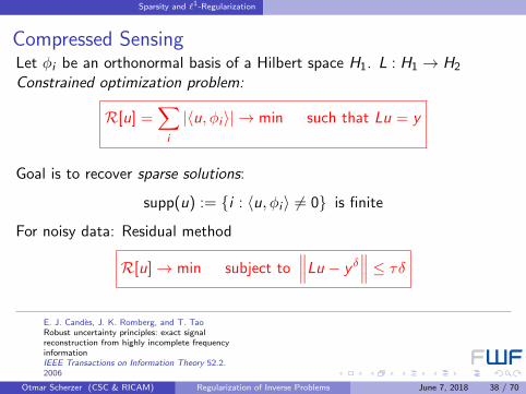
Compressed SensingLet φi be an orthonormal basis of a Hilbert space H1. L : H1 → H2
Constrained optimization problem:
R[u] =∑i
|〈u, φi 〉| → min such that Lu = y
Goal is to recover sparse solutions:
supp(u) := i : 〈u, φi 〉 6= 0 is finite
For noisy data: Residual method
R[u]→ min subject to∥∥∥Lu − y δ
∥∥∥ ≤ τδE. J. Candes, J. K. Romberg, and T. TaoRobust uncertainty principles: exact signalreconstruction from highly incomplete frequencyinformationIEEE Transactions on Information Theory 52.2.2006
Otmar Scherzer (CSC & RICAM) Regularization of Inverse Problems June 7, 2018 38 / 70
Sparsity and `1-Regularization
Compressed SensingLet φi be an orthonormal basis of a Hilbert space H1. L : H1 → H2
Constrained optimization problem:
R[u] =∑i
|〈u, φi 〉| → min such that Lu = y
Goal is to recover sparse solutions:
supp(u) := i : 〈u, φi 〉 6= 0 is finite
For noisy data: Residual method
R[u]→ min subject to∥∥∥Lu − y δ
∥∥∥ ≤ τδE. J. Candes, J. K. Romberg, and T. TaoRobust uncertainty principles: exact signalreconstruction from highly incomplete frequencyinformationIEEE Transactions on Information Theory 52.2.2006
Otmar Scherzer (CSC & RICAM) Regularization of Inverse Problems June 7, 2018 38 / 70

Sparsity and `1-Regularization
Sparsity Regularization
Unconstrained Optimization∥∥∥Lu − y δ∥∥∥2
+ αR[u]→ min
General theory for sparsity regularization:
Stability: y δ →H2 y ⇒ uδα H1 uα and∥∥uδα∥∥`1 → ‖uα‖`1
Convergence: y δ →H2 y ⇒ uδα H1 u† and∥∥uδα∥∥`1 →
∥∥u†∥∥`1 if
δ2/α→ 0.
If α is chosen according to the discrepancy principle, then SparsityRegularization ≡ Compressed Sensing
Otmar Scherzer (CSC & RICAM) Regularization of Inverse Problems June 7, 2018 39 / 70

Sparsity and `1-Regularization
Convergence Rates: Sparsity Regularization
Assumptions:
Source Condition: There exists η such that
H2 3 ξ = L∗η ∈ ∂R[u†] = ∂
(∑i
∣∣∣〈u†, φi 〉∣∣∣)
=∑i
sgn(〈u†, φi 〉)︸ ︷︷ ︸=:ξi
φi
⇒ u† is sparse (means in the domain of ∂R)
α ∼ δResult:
Dξ(uδα, u†) = O(δ) and
∥∥∥Luδα − y∥∥∥ = O(δ)
M. Grasmair, M. Haltmeier, and O. ScherzerNecessary and sufficient conditions for linearconvergence of l1-regularizationComm. Pure Appl. Math. 64.2. 2011
O. Scherzer, M. Grasmair, H. Grossauer,M. Haltmeier, and F. LenzenVariational methods in imagingSpringer, 2009
Otmar Scherzer (CSC & RICAM) Regularization of Inverse Problems June 7, 2018 40 / 70

Sparsity and `1-Regularization
Analogous Convergence Rates: Compressed Sensing
Assumption: Source condition
ξ = L∗η ∈ ∂R[u†]
ThenDξ(u∗, u
†) ≤ 2 ‖η‖ δ
for every
u∗ ∈ argminR[u] :
∥∥∥Lu − y δ∥∥∥ ≤ δ
Note: u∗ is the constraint solution
E. J. Candes, J. K. Romberg, and T. TaoRobust uncertainty principles: exact signalreconstruction from highly incomplete frequencyinformationIEEE Transactions on Information Theory 52.2.2006
M. Grasmair, M. Haltmeier, and O. ScherzerThe residual method for regularizing ill-posedproblemsAppl. Math. Comput. 218.6. 2011
Otmar Scherzer (CSC & RICAM) Regularization of Inverse Problems June 7, 2018 41 / 70

Sparsity and `1-Regularization
What can we deduce from the Bregman Distance?
Because we assume (φi )i∈N to be an orthonormal basis, the Bregmandistance simplifies to
Dξ(u, u†) = R[u]−R[u†]− 〈ξ, u − u†〉
= R[u]− 〈ξ, u〉
=∑i
(|〈u, φi 〉| − 〈ξ, φi 〉︸ ︷︷ ︸
=ξi
〈u, φi 〉︸ ︷︷ ︸=ui
)
Note, by the definition of the subgradient |〈ξ, φi 〉| ≤ 1
Otmar Scherzer (CSC & RICAM) Regularization of Inverse Problems June 7, 2018 42 / 70

Sparsity and `1-Regularization
Rates with respect to the norm: On the infinite set!Recall source condition ξ = L∗η ∈ ∂R[u†]Define
Γ(η) := i : |ξi | = 1 (which is finite – solution is sparse)
and the number (take into account that the coefficients of ζ are in `2)
mη := max |ξi | : i 6∈ Γ(η) < 1
ThenDξ(u∗, u
†) =∑i
|u∗,i | − ξiu∗,i ≥ (1−mη)∑
i 6∈Γ(η)
|u∗,i |
Consequently, since ‖·‖`1 ≥ ‖·‖`2 , we get∥∥∥∥∥∥∥πN\Γ(η)(u∗)− πN\Γ(η)(u†)︸ ︷︷ ︸=0
∥∥∥∥∥∥∥H1
≤ CDξ(u∗, u†) ≤ Cδ
Otmar Scherzer (CSC & RICAM) Regularization of Inverse Problems June 7, 2018 43 / 70

Sparsity and `1-Regularization
Rates with respect to the Norm: On the small Set
Additional Assumption: Restricted injectivity:
The mapping LΓ(η) is injective
Thus on Γ(η) the problem is well–posed on the small set and consequently∥∥∥πΓ(η)(u∗)− πΓ(η)(u†)∥∥∥H1
≤ Cδ
Together with previous slide:∥∥∥u∗ − u†∥∥∥H1
≤ Cδ
M. GrasmairLinear convergence rates for Tikhonovregularization with positively homogeneousfunctionalsInverse Probl. 27.7. June 2011
K. Bredies and D. LorenzLinear convergence of iterative soft-thresholdingJournal of Fourier Analysis and Applications14.5-6. 2008
Otmar Scherzer (CSC & RICAM) Regularization of Inverse Problems June 7, 2018 44 / 70

Sparsity and `1-Regularization
Restricted Isometry Property (RIP)Candes, Romberg, and Tao 2006: Key ingredient in proving linearconvergence rates for the finite dimensional `1-residual method:The s-restricted isometry constant ϑs of L is defined as the smallestnumber ϑ ≥ 0 that satisfies
(1− ϑ) ‖u‖2 ≤ ‖Lu‖2 ≤ (1 + ϑ) ‖u‖2
for all s-sparse u ∈ X . The (s, s ′)-restricted orthogonality constant ϑs,s′ ofL is defined as the smallest number ϑ ≥ 0 such that∣∣〈Lu, Lu′〉∣∣ ≤ ϑ ‖u‖ ∥∥u′∥∥for all s-sparse u and s ′-sparse u′ with supp(u) ∩ supp(u′) = ∅.The mapping L satisfies the s-restricted isometry property, ifϑs + ϑs,s + ϑs,2s < 1
E. J. Candes, J. K. Romberg, and T. TaoRobust uncertainty principles: exact signalreconstruction from highly incomplete frequencyinformationIEEE Transactions on Information Theory 52.2.2006
Otmar Scherzer (CSC & RICAM) Regularization of Inverse Problems June 7, 2018 45 / 70

Sparsity and `1-Regularization
Linear Convergence of Candes & Rhomberg & Tao
Assumptions:
1 L satisfies the s-restricted isometry property
2 u† is s-sparse
Result: ∥∥∥u∗ − u†∥∥∥H1
≤ csδ
However: These condition imply the source condition and the restrictedinjectivity
Otmar Scherzer (CSC & RICAM) Regularization of Inverse Problems June 7, 2018 46 / 70

Sparsity and `1-Regularization
0 < p < 1: Nonconvex sparsity regularization
∥∥∥Lu − y δ∥∥∥2
+ α∑|〈u, φi 〉|p → min
is stable, convergent, and well–posed in the Hilbert-space norm
Zarzer 2009: O(√δ)
Grasmair 2010b: ⇒ O(δ)
C. A. ZarzerOn Tikhonov regularization with non-convexsparsity constraintsInverse Problems 25. 2009
M. GrasmairNon-convex sparse regularisationJ. Math. Anal. Appl. 365.1. 2010
Otmar Scherzer (CSC & RICAM) Regularization of Inverse Problems June 7, 2018 47 / 70
Sparsity and `1-Regularization
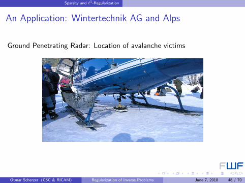
An Application: Wintertechnik AG and Alps
Ground Penetrating Radar: Location of avalanche victims
Otmar Scherzer (CSC & RICAM) Regularization of Inverse Problems June 7, 2018 48 / 70
Sparsity and `1-Regularization
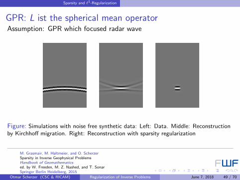
GPR: L ist the spherical mean operatorAssumption: GPR which focused radar wave
Figure: Simulations with noise free synthetic data: Left: Data. Middle: Reconstructionby Kirchhoff migration. Right: Reconstruction with sparsity regularization
M. Grasmair, M. Haltmeier, and O. ScherzerSparsity in Inverse Geophysical ProblemsHandbook of Geomathematicsed. by W. Freeden, M. Z. Nashed, and T. SonarSpringer Berlin Heidelberg, 2015
Otmar Scherzer (CSC & RICAM) Regularization of Inverse Problems June 7, 2018 49 / 70

Sparsity and `1-Regularization
GPR: Simulations with noisy data
Figure: Noisy data. Left: Data. Middle: Reconstruction by Kirchhoff migration. Right:Reconstruction with sparsity regularization
Otmar Scherzer (CSC & RICAM) Regularization of Inverse Problems June 7, 2018 50 / 70

Sparsity and `1-Regularization
Reconstruction with real data
Figure: Reconstruction from real data. Left: Data. Middle: Reconstruction byKirchhoff migration. Right: Reconstruction with sparsity regularization
Otmar Scherzer (CSC & RICAM) Regularization of Inverse Problems June 7, 2018 51 / 70

TV-Regularization
TV-Regularization
Let Ω,Σ two two open sets. TV minimization consists in calculating
uδα := argminu∈L2(Ω)
1
2
∥∥∥Lu − y δ∥∥∥2
L2(Σ)+ αTV [u]
L. I. Rudin, S. Osher, and E. FatemiNonlinear total variation based noise removalalgorithmsPhysica D. Nonlinear Phenomena 60.1–4. 1992
Otmar Scherzer (CSC & RICAM) Regularization of Inverse Problems June 7, 2018 52 / 70

TV-Regularization
TV-Regularization
Assumption: L is a bounded operator between L2(Ω) and L2(Σ)
Fact: TV is weakly lower semi-continuous on L2(Ω)
Results:
Stability: y δ →L2(Σ) y ⇒ uδα L2(Ω) uα and TV [uδα]→ TV [uα]
Convergence: y δ →L2(Σ) y and α = α(δ) such that δ2/α→ 0, then
uδα L2(Ω) u† and TV [uδα]→ TV [u†]
Otmar Scherzer (CSC & RICAM) Regularization of Inverse Problems June 7, 2018 53 / 70

TV-Regularization
TV-Regularization: Source Condition
u† satisfies the source condition if there exist ξ ∈ L2(Ω) and η ∈ L2(Σ)such that
ξ = L∗η ∈ ∂TV [u†]
Then for α ∼ δ
TV [uδα]− TV [u†]− 〈ξ, uδα − u†〉L2(Ω) = DξTV (uδα, u†) = O(δ)
M. Burger and S. OsherConvergence rates of convex variationalregularizationInverse Problems 20.5. 2004
O. Scherzer, M. Grasmair, H. Grossauer,M. Haltmeier, and F. LenzenVariational methods in imagingSpringer, 2009
Otmar Scherzer (CSC & RICAM) Regularization of Inverse Problems June 7, 2018 54 / 70

TV-Regularization
Source Condition for the Circular Radon TransformNotation: Ω := B(0, 1) ⊆ R2 open, ε ∈ (0, 1). We consider the CircularRadon transform
Scirc [u] := t
∫S1
u(z + tw)dH1(w)
for functions from
L2(B(0, 1− ε)) :=u ∈ L2(R2) : supp(u) ⊆ B(0, 1− ε)
is well-defined
bounded from L2(B(0, 1− ε)) into L2(S1 × (0, 1))
and ‖Scirc‖ ≤ 2π
O. Scherzer, M. Grasmair, H. Grossauer,M. Haltmeier, and F. LenzenVariational methods in imagingSpringer, 2009
Otmar Scherzer (CSC & RICAM) Regularization of Inverse Problems June 7, 2018 55 / 70
TV-Regularization
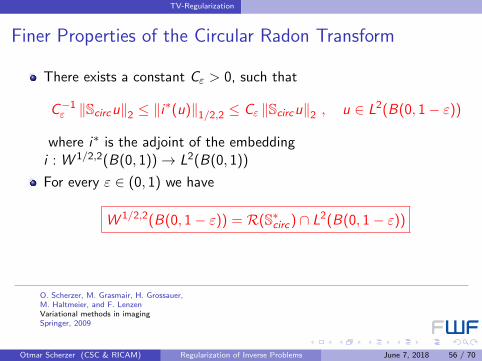
Finer Properties of the Circular Radon Transform
There exists a constant Cε > 0, such that
C−1ε ‖Scircu‖2 ≤ ‖i
∗(u)‖1/2,2 ≤ Cε ‖Scircu‖2 , u ∈ L2(B(0, 1− ε))
where i∗ is the adjoint of the embeddingi : W 1/2,2(B(0, 1))→ L2(B(0, 1))
For every ε ∈ (0, 1) we have
W 1/2,2(B(0, 1− ε)) = R(S∗circ) ∩ L2(B(0, 1− ε))
O. Scherzer, M. Grasmair, H. Grossauer,M. Haltmeier, and F. LenzenVariational methods in imagingSpringer, 2009
Otmar Scherzer (CSC & RICAM) Regularization of Inverse Problems June 7, 2018 56 / 70

TV-Regularization
Wellposedness of TV-minimization for Scirc
Minimization of the TV-functional with L = Scirc is
well-posed, stable, and convergent
Let ε ∈ (0, 1) and u† the TV -minimizing solution. Moreover, if theSource Condition
ξ ∈ ∂TV [u†] ∩W 1/2,2(B(0, 1− ε))
is satisfied, then
TV [uδα]− TV [u†]− 〈ξ, uδα − u†〉 = O(δ)
Otmar Scherzer (CSC & RICAM) Regularization of Inverse Problems June 7, 2018 57 / 70

TV-Regularization
Functions that satisfy the Source Condition
Let ρ ∈ C∞0 (R2) be an adequate mollifier and ρµ the scaled functionof ρ. Moreover, let x0 = (0.2, 0), a = 0.1, and µ = 0.3. Then
u† := 1B(x0,a+µ) ∗ ρµ
satisfies the source condition
Let u† := 1F be the indicator function of a bounded subset of R2
with smooth boundary
Otmar Scherzer (CSC & RICAM) Regularization of Inverse Problems June 7, 2018 58 / 70

TV-Regularization
Convergence of Level-Sets
Ω ⊂ R2!
1
2
∥∥∥Lu − y δ∥∥∥2
L2(Σ)+ αTV [u]→ min
foru ∈ L2(Ω) ∼=
u ∈ L2(R2) : supp(u) ⊂ Ω
A. Chambolle, V. Duval, G. Peyre, and C. PoonGeometric properties of solutions to the totalvariation denoising problemInverse Problems 33.1. 2017
J. A. Iglesias, G. Mercier, and O. ScherzerA note on convergence of solutions of totalvariation regularized linear inverse problemsInverse Probl. 35.5. 2018
Otmar Scherzer (CSC & RICAM) Regularization of Inverse Problems June 7, 2018 59 / 70
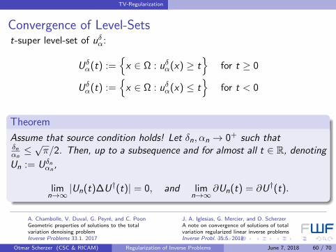
TV-Regularization
Convergence of Level-Setst-super level-set of uδα:
Uδα(t) :=
x ∈ Ω : uδα(x) ≥ t
for t ≥ 0
Uδα(t) :=
x ∈ Ω : uδα(x) ≤ t
for t < 0
Theorem
Assume that source condition holds! Let δn, αn → 0+ such thatδnαn≤√π/2. Then, up to a subsequence and for almost all t ∈ R, denoting
Un := Uδnαn
,
limn→∞
|Un(t)∆U†(t)| = 0, and limn→∞
∂Un(t) = ∂U†(t).
A. Chambolle, V. Duval, G. Peyre, and C. PoonGeometric properties of solutions to the totalvariation denoising problemInverse Problems 33.1. 2017
J. A. Iglesias, G. Mercier, and O. ScherzerA note on convergence of solutions of totalvariation regularized linear inverse problemsInverse Probl. 35.5. 2018
Otmar Scherzer (CSC & RICAM) Regularization of Inverse Problems June 7, 2018 60 / 70

TV-Regularization
A Deblurring Result
Figure: Deblurring of a characteristic function by total variation regularization withDirichlet boundary conditions. First row: Input image blurred with a known kernel andwith additive noise. Second row: numerical deconvolution results. Third row: some levellines of the results.
Otmar Scherzer (CSC & RICAM) Regularization of Inverse Problems June 7, 2018 61 / 70

Regularization of High-Dimensional Data
Image Registration: Model Problems
Given: Images I1, I2 : Ω ⊆ R2 → RFind u : Ω→ Ω satisfying
L[u] := I2 u = I1
u should be a diffeomorphism (no twists)
Otmar Scherzer (CSC & RICAM) Regularization of Inverse Problems June 7, 2018 62 / 70

Regularization of High-Dimensional Data
Calculus of Variations: Notions of Convexity
f : Rm × Rn × Rm×n → R ,(x , u, v)→ f (x , u, v)
Hierarchy:
f convex ⇒ polyconvex ⇒ quasi-convex ⇒ rank-one convex
Up to quasi-convexity:
u →∫Rm
f (x , u,∇u) dx is weakly lower semicontinuous on
H1 := W 1,p(Ω,Rn) with 1 ≤ p ≤ ∞If m = 1 or n = 1, then all convexity definitions are equivalentPolyconvex functionals are used in elasticity theory
C. B. MorreyMultiple Integrals in the Calculus of VariationsSpringer Verlag, 1966
B. DacorognaDirect Methods in the Calculus of VariationsSpringer Verlag, 1989
Otmar Scherzer (CSC & RICAM) Regularization of Inverse Problems June 7, 2018 63 / 70

Regularization of High-Dimensional Data
Polyconvex FunctionsFor A ∈ Rm×n and 1 ≤ s ≤ m ∧ n
adjs(A) consists of all s × s minors of A (subdeterminants)
f : Rm×n → R ∪ +∞ is polyconvex if
f = F T ,
where F : Rτ(m,n) → R ∪ +∞ is convex and
T : Rm×n → Rτ(m,n) , A→ (A, adj2(A), . . . , adjτ(m,n)(A))
Typical example:f (A) = (det[A])2
J. M. BallConvexity conditions and existence theorems innonlinear elasticityArchive for Rational Mechanics and Analysis 63.1977
Otmar Scherzer (CSC & RICAM) Regularization of Inverse Problems June 7, 2018 64 / 70

Regularization of High-Dimensional Data
Polyconvex Regularization
Assumptions:
R[u] :=∫
Ω F T [u](x) dx .
L is a non-linear continous operator between W 1,p(Ω,Rn) and H2
(sometimes needs to be a Banach space) with closed and convexdomain of definition D(L)
Results:
Stability: y δ →H2 y ⇒ uδα W 1,p uα and R[uδα]→ R[uα]
Convergence: y δ →H2 y and α = α(δ) such that δ2/α→ 0, then
uδα W 1,p u† and R[uδα]→ R[u†]
Otmar Scherzer (CSC & RICAM) Regularization of Inverse Problems June 7, 2018 65 / 70

Regularization of High-Dimensional Data
Generalized Bregman Distances
Let W be a family of functionals on H1 = W 1,p(Ω,Rn)
The W-subdifferential of a functional R is defined by
∂WR[u] = w ∈W : R[v ] ≥ R[u] + w [v ]− w [u] , ∀v ∈ H1
For w ∈ ∂WR[u] the W -Bregman distance is defined by
DWw (v , u) = R[v ]−R[u]− w [v ] + w [u]
M. GrasmairGeneralized Bregman distances and convergencerates for non-convex regularization methodsInverse Probl. 26.11. Oct. 2010
I. SingerAbstract convex analysisJohn Wiley & Sons Inc., 1997
Otmar Scherzer (CSC & RICAM) Regularization of Inverse Problems June 7, 2018 66 / 70

Regularization of High-Dimensional Data
Bregman Distances of Polyconvex IntegrandsLet p ∈ [1,∞) and H1 = W 1,p(Ω,Rn).
T (∇u) ∈m∧n∏s=2
Lps (Ω,Rσ(s)) =: S2.
We define
Wpoly := w : H1 → R : ∃(u∗, v∗) ∈ H∗1 × S∗2 s.t.
w [u] = 〈u∗, u〉H∗1 ,H1 + 〈v∗,T (∇u)〉S∗2 ,S2
Remark:
Wpoly = (H1 × S2)∗. However, functionals w are non-linear
Wpoly-Bregman distance:
Dpolyw (u, u) = R[u]−R(u)− w [u] + w(u)
= R[u]−R(u)− 〈u∗, u − u〉H∗1 ,H1
− 〈v∗,T (∇u)− T (∇u)〉S∗2 ,S2
Otmar Scherzer (CSC & RICAM) Regularization of Inverse Problems June 7, 2018 67 / 70

Regularization of High-Dimensional Data
Polyconvex Subgradient
Ω ⊂ Rm and H1 = W 1,p(Ω,Rn)
For x ∈ Ω, the map (u,A) 7→ F (x , u,A) is convex and differentiable
R[u] =∫
Ω F (x , u(x),T (∇u(x)))dx
Definition
If R[v ] ∈ R and the function x 7→ F ′u,A(x , v(x),T (∇v(x))) lies in
Lp∗(Ω,Rn)×
m∧n∏s=1
Lps (Ω,Rσ(s)),
then this function is a Wpoly-subgradient of R at v
Otmar Scherzer (CSC & RICAM) Regularization of Inverse Problems June 7, 2018 68 / 70
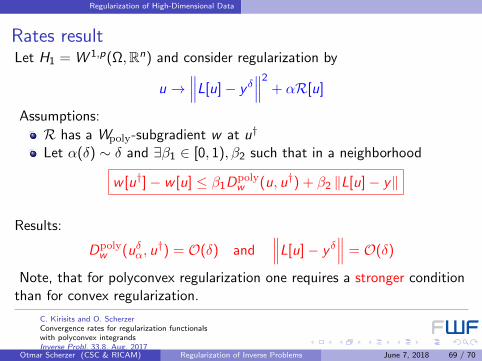
Regularization of High-Dimensional Data
Rates resultLet H1 = W 1,p(Ω,Rn) and consider regularization by
u →∥∥∥L[u]− y δ
∥∥∥2+ αR[u]
Assumptions:
R has a Wpoly-subgradient w at u†
Let α(δ) ∼ δ and ∃β1 ∈ [0, 1), β2 such that in a neighborhood
w [u†]− w [u] ≤ β1Dpolyw (u, u†) + β2 ‖L[u]− y‖
Results:
Dpolyw (uδα, u
†) = O(δ) and∥∥∥L[u]− y δ
∥∥∥ = O(δ)
Note, that for polyconvex regularization one requires a stronger conditionthan for convex regularization.
C. Kirisits and O. ScherzerConvergence rates for regularization functionalswith polyconvex integrandsInverse Probl. 33.8. Aug. 2017
Otmar Scherzer (CSC & RICAM) Regularization of Inverse Problems June 7, 2018 69 / 70
Regularization of High-Dimensional Data
Thank you for your attention
Otmar Scherzer (CSC & RICAM) Regularization of Inverse Problems June 7, 2018 70 / 70