regularization-based fictitious domain...
TRANSCRIPT
Regularization-Based Fictitious
Domain Methods
DISSERTATION
zur Erlangung des Grades eines Doktors
der Naturwissenschaften
vorgelegt von
Dipl.-Math. Torsten Kruger
eingereicht bei der Naturwissenschaftlich-Technischen Fakultat
der Universitat Siegen
Siegen 2012

Gutachter der Dissertation: Professor Dr. Franz-Theo Suttmeier
Professor Dr. Robert Plato
Tag der mundlichen Prufung: 31.10.2012
Gedruckt auf alterungsbestandigem holz- und saurefreiem Papier.

Zusammenfassung
Die vorliegende Arbeit befasst sich mit Methoden aus dem Bereich der sogenannten
Fictitious Domain (FD) Techniken bei gleichzeitiger Verwendung von Finiten Ele-
menten. Fictitious Domain Techniken eigenen sich gut, falls das Gebiet, auf dem
eine partielle Differenzialgleichung gelost werden soll, geometrisch komplex oder
auch zeitabhangig ist.
Eigene Vorschlage, welche auf Straf- und Regularisierungstechniken basieren, wer-
den vorgestellt und analysiert. Varianten der bekannten Nitsche-Methode zur
Aufpragung von Randbedingungen kommen zum Einsatz. Dies wird kombiniert
mit Verfahren einer regularisierungs-basierenden FD Methode, ursprunglich erdacht
von Glowinski et al.
Die zugrunde liegenden Modellgleichungen zweiter Ordnung sind dabei von nicht-
linearer und recht allgemeiner Natur. Eine numerische Analyse findet in Bezug
auf die linearisierten Gleichungen statt. So wird neben den resultierenden sym-
metrischen Problemen insbesondere auch auf Aspekte hinsichtlich dominanter Kon-
vektion eingegangen, sowie auf die Umgehung einer diskreten Inf-Sup-Bedingung im
Falle des Oseen-Problems. Der Nutzung von Streamline-Diffusion/Galerkin-Least-
Squares Techniken kommt dabei die Schlusselrolle zu.
Die erforderliche implizite Beschreibung der ursprunglichen Geometrie erfolgt uber
die Level Set Methode. Dabei wird der eingebettete Rand als Nullmenge einer
geeigneten Funktion beschrieben, was eine bequeme und flexible Handhabung der
Geometrie erlaubt.
Der Darstellung von zugrunde liegenden algorithmischen Aspekten und einer allge-
meinen Uberprufung hinsichtlich der Genauigkeit der neuen Methoden anhand von
verschiedenen Beispielen mit bekannter analytischer Losung wird Platz eingeraumt.
Teil der Arbeit ist zudem die Prasentation verschiedener Anwendungen, um das
Potenzial der neuen Methoden auf verschiedenen Gebieten auszuloten. Dazu
werden Beispiele aus dem Bereich der planaren stationaren und instationaren
Stromungsprobleme, inklusive einem Beispiel mit bewegtem Rand, sowie die Bouss-
inesq-Gleichungen auf komplexen, mehrfach zusammenhangenden Gebieten, behan-
delt.

Summary
The work at hand is addressed to methods from the fictitious domain context, com-
bined with the finite element method. Fictitious domain techniques are suitable in
case partial differential equations have to be solved on a geometrically complex or
time-dependent domain.
Own suggestions based on penalization and regularization, utilizing variants of
Nitsches method in order to impose boundary conditions in a weak sense, are intro-
duced and analyzed. The techniques presented are generalizations of methods due
to Glowinski et al.
The underlying model equations of order two are non-linear reaction-diffusion-
convection equations of rather general type, able to describe a lot of real-world
situations. In addition, incompressible Stokes and Navier-Stokes systems are intro-
duced, being special cases of the original model equations in some sense.
The numerical analysis is carried out with respect to linearized versions of the origi-
nal model equations. Within this process, symmetrical reaction-diffusion, diffusion-
convection-reaction and a version of the Oseen equations are treated separately, in
order to deal with different typical problems appearing in each case adequately.
Following that, besides symmetrical problems, tasks like dominant convection, as
well as the circumvention of a discrete inf-sup condition in case the Oseen problem
are discussed. Streamline diffusion/Galerkin least squares techniques playing a key
role in that matter.
For implicit description of the embedded boundary the well established level set
method is used, describing the boundary as a zero level set of suitable functions.
This allows for an easy and flexible handling of the geometrical aspects.
Algorithmic tasks are addressed, followed by tests regarding numerical accuracy. In
the end, several applications are presented in order to show the potential of the
new methods: Examples regarding plain flow problems, including one with moving
boundary, and the Boussinesq equations on complex multi-connected domains.

Contents
1 Introduction 1
2 Description of the model equations 5
2.1 Nomenclature and basic principles . . . . . . . . . . . . . . . . . . . . 5
2.2 Reaction-Diffusion-Convection (RDC) equations . . . . . . . . . . . . 9
2.2.1 Classical formulation . . . . . . . . . . . . . . . . . . . . . . . 9
2.2.2 Weak formulation . . . . . . . . . . . . . . . . . . . . . . . . . 10
2.3 Stokes and Navier-Stokes equations . . . . . . . . . . . . . . . . . . . 11
2.3.1 Classical formulation . . . . . . . . . . . . . . . . . . . . . . . 11
2.3.2 Weak formulation . . . . . . . . . . . . . . . . . . . . . . . . . 12
2.4 Fictitious Domain (FD) method . . . . . . . . . . . . . . . . . . . . . 14
2.4.1 General concept of FD and related methods . . . . . . . . . . 16
2.4.2 Scalar problem with mixed boundary conditions . . . . . . . . 21
2.4.3 Fictitious Domain Oseen problem . . . . . . . . . . . . . . . . 26
2.5 Description of domain geometries . . . . . . . . . . . . . . . . . . . . 28
3 Discretization 31
3.1 Assumptions on domain and triangulation . . . . . . . . . . . . . . . 32
3.2 FD discretization for the scalar model equation . . . . . . . . . . . . 34
3.2.1 Stability of the discrete form . . . . . . . . . . . . . . . . . . . 38
3.2.2 Stabilization in the convection dominated case . . . . . . . . . 40
3.2.3 A priori error in the symmetric case . . . . . . . . . . . . . . . 43
3.2.4 A priori error for the stabilized method . . . . . . . . . . . . . 47
3.3 FD discretization of the Oseen problem . . . . . . . . . . . . . . . . . 50
3.3.1 Stability of the discrete form . . . . . . . . . . . . . . . . . . . 51
3.3.2 A priori error in the symmetric case . . . . . . . . . . . . . . . 61
3.4 Time discretization . . . . . . . . . . . . . . . . . . . . . . . . . . . . 64
4 Numerical treatment 67
i
Contents
4.1 Approximation of the domain Ω and local integration . . . . . . . . . 67
4.2 A geometrical regularization method . . . . . . . . . . . . . . . . . . 71
4.3 Non-linear defect correction . . . . . . . . . . . . . . . . . . . . . . . 72
4.4 Numerical accuracy . . . . . . . . . . . . . . . . . . . . . . . . . . . . 74
5 Applications 85
5.1 Application I: Steady laminar flow around a plain cylinder . . . . . . 85
5.1.1 Problem setting . . . . . . . . . . . . . . . . . . . . . . . . . . 86
5.1.2 Numerical details . . . . . . . . . . . . . . . . . . . . . . . . . 87
5.1.3 Benchmark quantities . . . . . . . . . . . . . . . . . . . . . . . 88
5.1.4 Results and observations . . . . . . . . . . . . . . . . . . . . . 89
5.2 Application II: Non-steady flow around a plain cylinder . . . . . . . . 93
5.2.1 Problem setting . . . . . . . . . . . . . . . . . . . . . . . . . . 93
5.2.2 Numerical details . . . . . . . . . . . . . . . . . . . . . . . . . 94
5.2.3 Results and observations . . . . . . . . . . . . . . . . . . . . . 95
5.3 Application III: Boussinesq equations on multi-connected domains. . 98
5.3.1 Description of the problem . . . . . . . . . . . . . . . . . . . . 98
5.3.2 Numerical details . . . . . . . . . . . . . . . . . . . . . . . . . 100
5.3.3 Results and observations . . . . . . . . . . . . . . . . . . . . . 102
5.4 Application IV: Incompressible viscous flow around a moving plain
cylinder . . . . . . . . . . . . . . . . . . . . . . . . . . . . . . . . . . 108
5.4.1 Problem setting . . . . . . . . . . . . . . . . . . . . . . . . . . 108
5.4.2 Numerical details . . . . . . . . . . . . . . . . . . . . . . . . . 109
5.4.3 Results and observations . . . . . . . . . . . . . . . . . . . . . 110
6 Discussion and Outlook 113
Bibliography 115
ii

1 Introduction
Motivation and Objectives
In many fields, like fluid dynamics and elasticity, problems occur making it necessary
to solve problems on domains being geometrically complex or time-dependent. As
the generation of boundary-fitted meshes of good quality in such cases is a rather
complex, often time consuming task of (not at least from the computational point of
view) high cost, the fictitious domain (FD) method (see [Glo03]) and other related
methods have been developed in order to overcome the meshing and re-meshing
problem. This is done by embedding the original problem stated on a domain
Ω ⊂ Rd into a simple shaped domain Ω, in many cases chosen as a parallelepiped of
equal dimension. After that, the triangulation is carried out for the larger domain
Ω, which has a rather Eulerian character, and is not fitted to the boundary of Ω ⊂ Ω
in general. The original problem then is replaced by a new, being related to the
original one, with the resulting solution restricted to Ω being at least close to the
solution of the original problem in some sense.
The actual work at hand jumps on that bandwagon by presenting new variants of
methods in the FD context, based on regularization, to overcome the problems stem-
ming from ill-posedness of the problems on the fictitious domain, and those following
from the necessity of imposing additional essential constraints on the solution. The
level set method (see [Set99]) is used to describe the domain Ω implicitly rather than
explicitly by a boundary-fitted mesh. We follow the papers of Pan and Glowinski et
al. [GPWZ96,GP92], in order to develop and analyse methods being generalizations
of the one stated in the mentioned papers, to the cases of far more general time-
dependent, non-linear reaction-diffusion-convection problems with mixed boundary
conditions, as well as the case of Stokes and Navier-Stokes systems describing in-
compressible fluid flow. Various numerical tests and applications are given in order
to demonstrate and evaluate the new methods under consideration.
The aim is to present methods being able to handle problems without introducing
1
1 Introduction
additional degrees of freedom, which is a common way in the fictitious domain
community, but just using standard finite element spaces and meshes. Moreover,
the philosophy of the methods at hand is to handle the problems in a quit standard
way on the domain Ω, employing techniques like Galerkin least squares stabilization
(e.g. [RST08]) in order to deal with additional problems like dominant convection
and violation of a discrete inf-sub condition in case of saddle point problems and
mixed finite elements (cf. [BF91]).
As a first demonstration and motivation, an example of Navier-Stokes flow around
multiple obstacles in case of a lid-driven cavity is shown in Figure 1.1. The ficti-
tious domain techniques presented in this work are used for the simulation, with a
Cartesian grid covering (−1, 1)2 as a fictitious domain. While it would be standard
to generate a triangulation in case of a single inner circle, as such kind of holed do-
mains are contained in every ordinary grid-generator, it would be harder to generate
a suitable fitted mesh in case of the multi-obstacle flow. That case would make it
necessary to build up a new grid, using a mesh-generator or by hand in an suitable
format, if there was not a good soul having already implemented such a structure,
which in general would be surprising. Not to mention the case the obstacles would
change the number or shape and/or move in time. With the methods at hand han-
dling such problems is not hard in principle, as only an implicit description has to be
given for the position of the obstacles, avoiding complicated meshing an re-meshing
procedures.
Outline of the thesis
The outline after the introduction is as follows:
- In the second chapter, the continuous context, including the nomenclature and
basic principles, as well as the underlying general linear and non-linear prob-
lems is given. This is done along with a review of FD methods and related
ones already existing. The new methods, being generalizations of the one pre-
sented in [GPWZ96,GP92], are introduced in the continuous context, based on
suitable model problems being linearized versions of the firstly presented non-
linear equations. Furthermore, methods fit for describing a domain implicitly
are discussed, with the level set method among them.
- The third chapter is addressed to the discretization of the continuous case,
with special attention on formulating well-posed discrete problems. The latter
2

Figure 1.1: Example of a lid-driven cavity flow around multi-obstacles modelled bythe Navier-Stokes equations. The regularized fictitious domain methodspresented in this work have been used for solving the system of equations.
in general is not an easy task, as one has to deal with grids not fitted to the
boundary of the underlying domain. Numerical robustness in case of singularly
perturbed equations is discussed. Variants of Nitsches method (see [Nit71])
are the methods of choice in order to enforce essential Dirichlet boundary
conditions, while streamline diffusion/Galerkin least squares techniques are
brought into play for stabilization. The methods are given and analysed for
linear scalar model problems and vectorial Oseen problems, as both types of
equations need different treatment to show the methods result in well-posed
problems.
- Implementational and algorithmic issues are presented in the fourth chap-
ter : Linearization techniques, local quadrature, the solution process and for
completeness an additional geometrical regularization. As the basis for imple-
mentation, the free finite element C++-library deal.II, see [BHK07], is used.
The chapter ends with the presentation of test problems for evaluating the
accuracy of the methods.
- The fifth chapter gives some practical applications:
a) Laminar flow around a plain cylinder, which is an essential benchmark
problem, as a lot of numerical and experimental data are available, show-
ing that our new methods work accurate, while being able to handle
steady flow problems,
3

1 Introduction
b) Unsteady flow around a plain cylinder, another benchmark for testing
whether a solver works accurate and is able to resolve non-linear effects,
while leaving the laminar regime. As it turns out the solver based on
the new FD based methods is able to produce sufficiently good results
compared to established boundary-fitted methods,
c) Exploring the capabilities of the new methods to treat with the time-
dependent Boussinesq equations on multi-connected domains. Which
turns out to give qualitatively good results with respect to physical phe-
nomena, while at the same time the accurate enforcing of strong con-
straints at the inner boundaries of the domain in the considered laminar
regime is ensured. Moreover, the high flexibility regarding geometrical
complex stationary domains is shown,
d) Time-dependent incompressible viscous flow around a moving plain cylin-
der, in order to show the method is able to deal with moving boundary
problems in principle. This is another test the new methods pass, while
the description of the method is not perfectly adequate from the physical
and mathematical point of view with no further modification regarding
the time derivative. Nevertheless, from the qualitative side the methods
gives sufficient results compared to other FD methods.
Finally, the work is ended by the discussion and outlook section, highlighting pros
and cons of the new methods, along with giving hints for further improvements and
interesting fields to be explored using the methods developed in this work.
4

2 Description of the model equations
In this chapter the model equations treated in this work are introduced. We want
to deal with systems of non-linear reaction-diffusion-convection (RDC) equations,
in order to be able to cover a wide range of problems in a uniform framework. The
aim is to give a general background, not to focus on the solvability of this partial
differential equation (PDE) systems. Doing so, we present the basic principles and
the nomenclature used in this work, as well as the general appearance of the equa-
tions and terms we have to deal with. As complicated and maybe time dependent
domains have to be considered, furthermore a journey on the treatment of weakly
imposed boundary conditions in the case of a mesh not fitted to the boundary of the
domain the equations are defined on, is given. Finally we present own ideas in this
context, based on regularization techniques first time given in [GP92]. The chapter
is ended by discussing techniques for implicit description of a given domain.
2.1 Nomenclature and basic principles
Within this paragraph the basic principles and the nomenclature of this work are
presented in a compact fashion. In what follows let Ω ⊂ Rd (d = 2, 3) always
be a connected, open and bounded domain with a rectifiable, sufficiently smooth
boundary Γ := ∂Ω, i.e. Γ being of class Ck,1 for some integer k ≥ 0.
Definition 2.1 (see [AH09]). Let V be a function space on Rd−1. Γ is of class V ,
if for each point x0 ∈ Γ there exists an r > 0, as well as a function g ∈ V , such that
we have
Ω ∩ Br(x0) = x ∈ Br(x0) : xd > g(x1, . . . , xd−1) ,
upon a transformation of the coordinate system if necessary.
Here Br(x0) is the open d-dimensional ball with radius r and center x0. In particular,
if the function space V consists of Ck functions, we say Ω is of class Ck or simply
5
2 Description of the model equations
a Ck domain. If the function space V consists of Ck,1 functions, that is functions
with k-times Lipschitz continuous partial derivatives, we say Ω is of class Ck,1, or
Ω is a Lipschitz domain (of class Ck,1), or simply a Ck,1 domain.
The unit normal vector pointing outward in some point x (in what follows not
written in bold letters) of the boundary is denoted by n = n(x). Let always be
I := (0, T ) ⊂ R a time interval, T > 0 and t ∈ I. In general the domain could be
time-dependent (Ω = Ω(t)) as well.
The normal derivatives ∂nu and ∂nu are defined to be
∂nu := n · ∇u, ∂nu := (n · ∇)u = (∂nui)i=1,...,d
in the vectorial case.
The Lebesgue measure of a subset X ⊂ Rm is written as
meas(X) :=
∫Rm
1X dX, where 1X(x) :=
1 if x ∈ X,
0 else.
We will denote the standard inner product of the Hilbert space L2(X) over the real
numbers, with elements defined on a bounded domain X ⊂ Rd, for scalar functions
u, v ∈ L2(X) by
(u, v)X :=
∫X
uv dx,
and
(u,v)X :=d∑i=1
(ui, vi)X , (U ,V )X :=d∑
i,j=1
(Uij, Vij)X ,
in the case of u,v being elements of (L2(X))d
and U ,V ∈ (L2(X))d×d
, with the
corresponding component functions indexed.
Moreover, in case of X ⊂ Rd−1 the inner product of L2(X) is denoted by
〈u, v〉X :=
∫X
uv ds, 〈u,v〉X :=d∑i=1
〈ui, vi〉X ,
analogous to the former cases. The induced L2(X)-norms are then denoted by
‖ · ‖0,X := (·, ·)12X or ‖ · ‖0,X := 〈·, ·〉
12X ,
6
2.1 Nomenclature and basic principles
depending on the context.
Besides that, for X ⊂ Rd and p ∈ [1,∞], we denote the Lp(X)-norm of a suitable
function v (analogous in case of vector or matrix functions) by
‖v‖Lp(X) :=
(∫X
|v|p) 1
p
and ‖v‖L∞(X) := ‖v‖∞,X := infmeas(X′)=0
supx∈X\X′
|v(x)|.
Following that, it holds ‖v‖L2(X) = ‖v‖0,X in case v ∈ L2(X).
Definition 2.2. Let k be a non-negative integer, p ≥ 1 a real number. The Sobolev
space W k,p(X), X ⊂ Rd open and bounded, is defined to be
W k,p(X) :=v ∈ Lp(X) : ∂αv ∈ Lp(X), |α| ≤ k
,
with α a multi-index. The space shall be equipped with the norm and semi-norm
‖v‖k,p,X :=
∑|α|≤k
‖∂αv‖20,X
12
, |v|k,p,X :=
∑|α|=k
‖∂αv‖20,X
12
.
It is a well-known fact that W k,p(X) is a Banach space.
The case p = 2 is very important when dealing with second order problems. As it
is common practice, we will make use of the Sobolev spaces Hk(X) := W k,2(X),
X ⊂ Rd open and bounded, for some integer k > 0.
Definition 2.3. Let k be a non-negative integer. The space Hk(X) := W k,2(X)
shall be equipped with the norm and semi-norm
‖v‖k,X := ‖v‖k,2,X , |v|k,X := |v|k,2,X
and the inner product
(u, v)k,X :=∑|α|≤k
(∂αu, ∂αv)0,X , u, v ∈ Hk(X).
Another well-known fact is the next theorem, see e.g. [Hac86] and [Bra03].
7

2 Description of the model equations
Theorem 2.1. Assume Ω ⊂ Rd is a Lipschitz domain. Then there exists a contin-
uous linear operator γ : H1(Ω)→ L2(Γ) with
(a) γv = v|Γ if v ∈ H1(Ω) ∩ C(Ω).
(b) ∃C = C(Ω) > 0 : ‖γv‖0,Γ ≤ C‖v‖1,Ω ∀v ∈ H1(Ω).
(c) γ is a compact mapping.
Using this trace operator, the Sobolev space H12 (Γ) is defined as
H12 (Γ) := w ∈ L2(Γ) : ∃v ∈ H1(Ω) : w = γv,
equipped with the norm
‖w‖ 12,Γ := inf‖v‖1,Ω : v ∈ H1(Ω), γv = w.
Furthermore, by the trace operator the closed subspace:
H10 (Ω) :=
v ∈ H1(Ω) : γ(v) = v|Γ = 0
⊂ H1(Ω).
can be specified.
Let now the boundary be partitioned into Γ1 and Γ2, with Γ = Γ1∪Γ2 and Γ1∩Γ2 = ∅,where Γ1 is relatively closed, Γ2 relatively open. The cases Γ1 = ∅ or Γ2 = ∅ shall be
allowed as well. In the case of Γ1 6= ∅ it can be shown, that there exists an analogous
continuous trace operator γ1 : H1(Ω)→ L2(Γ1) with γ1v = v|Γ1 , see [Glo03,QV94].
In this sense, for suitable functions g, gi ∈ C∞(Ω) ∩ H1(Ω) mapping to R, g =
(gi)i=1,...,d, we define for frequently usage:
Vg(Ω) :=v ∈ H1(Ω) : v|Γ1 = g
,
Vg(Ω) :=v ∈
(H1(Ω)
)d: v|Γ1 = g
.
In order to get convergence results for the methods presented later on, it will be
necessary to extend the solution of the problems we want to treat onto a domain
covering the original one. An interesting and also well known statement, suitable for
this purpose, is given in Theorem 2.2. It is a basic result regarding the existence of an
extension operator in case of sufficiently smooth functions and domain boundaries.
8
2.2 Reaction-Diffusion-Convection (RDC) equations
Theorem 2.2 (see [GT83]). Let k ≥ 0 be an integer and Ω ⊂ Rd be a bounded Ck,1
domain with Ω ⊂ Ω, Ω being an open set in Rd. Then there exists a bounded linear
extension operator Ek+1 : Hk+1(Ω)→ Hk+1(Ω) such that Ek+1v|Ω = v and
‖Ek+1u‖k+1,Ω ≤ C(k,Ω, Ω)‖u‖k+1,Ω ∀v ∈ Hk+1(Ω). (2.1)
2.2 Reaction-Diffusion-Convection (RDC) equations
Motivated by physical processes and applications like reactive flow, droplet evapo-
ration and other complex systems, we want to model the transport of one or several
quantities wi within an open, time-dependent domain, driven by diffusion and/or a
flow field. Reactions between these quantities should be allowed as well.
As we will specify the terms for special cases in the application parts later on, we
will now state the general type of non-linear coupled second order partial differential
equation systems with possibly mixed Dirichlet and Neumann boundary data we
want to deal with.
2.2.1 Classical formulation
Splitting the boundary Γ = ∂Ω into the disjoint sets Γ = ΓD∪ΓN , with ΓD∩ΓN = ∅,the classical formulation of the problems we want to treat is stated to be:
∂twi −∇ · ji + β · ∇wi = ri + fi in Ω× I, (2.2)
wi = giD on ΓD × I, (2.3)
ji ∂nwi = giN on ΓN × I, (2.4)
wi(x, 0) = wi0 on Ω. (2.5)
The cases ΓD = ∅ or ΓN = ∅ are allowed as well.
The index i runs from 1 to N , with N being the total number of quantities wi under
consideration. For the vector valued flux functions ji we suppose that there holds
ji = ji∇wi.
9

2 Description of the model equations
In this general formulation ri, ji are sufficiently smooth scalar functions, typically
depending on
w = (wi)i=1,...,n
and/or the space coordinate x and time coordinate t:
ri = ri(x, t,w), ji = ji(x, t,w).
Neumann and Dirichlet data are supposed to be functions in space and time, but in
general could be depending on w as well:
giN = giN(x, t,w), giD = giD(x, t,w).
Physically the ji stands for the individual diffusive flux of the ith quantity, and so
the term including the ji stands for the diffusive part, also taking into account the
influence of the remaining quantities on the diffusive processes of ith quantity. The
ri-terms model the reactions between the ith quantity and the rest of the system.
The fi represents an external force, taking effect on the ith quantity, this functions
sufficiently smooth as well.
The data β : Ω × I → Rd is an external velocity field which models convection
within the system. This velocity field will be calculated from a Stokes or Navier-
Stokes system (see next subsection) in many cases, but it could be of complete
external origin. In many cases the convective part will dominate the equations.
2.2.2 Weak formulation
Testing with appropriate functions from V0(Ω) and integrating by parts yields the
weak form corresponding to our problem (1.2)-(1.5). Our weak formulation thus
reads:
For i = 1, . . . , N and t ∈ I find wi(t) ∈ VgiD(Ω), with wi(·, 0) = wi0(·), such that:
(∂twi, v)Ω + ai(w; v) = (hi(w); v) (2.6)
for all v ∈ V0(Ω).
10

2.3 Stokes and Navier-Stokes equations
The semi-linear forms are defined as:
ai(w; v) := (ji,∇ϕ)Ω + (β · ∇wi, v)Ω, (2.7)
(hi(w); v) := (ri, v)Ω + (fi, v)Ω + 〈giN , v〉ΓN . (2.8)
Clearly, this system in general does not have a solution, we will focus on such cases
a solution exists.
In particular we will have to treat linearized versions of the system under the typical
assumptions ensuring the solvability due to the Lax-Milgram theorem in the linear
case. These assumptions will be discussed in another section, which treats a (linear)
model problem closely related to the general (stationary) system, and we will assume
that analogue and directly transferable assumptions always hold in the considered
problems.
Remark 2.1. In case the diffusion coefficient depends on derivatives of w, it may
be necessary to substitute the underlying H1(Ω)-space by W 1,p(Ω), with suitable
p in the definition of VgiD(Ω), in order to match the smoothness properties of the
solution. An example for this is the well known p-Laplace problem and other akin
ones. Similar will be true in case of the Stokes and Navier-Stokes problem later on.
2.3 Stokes and Navier-Stokes equations
In order to handle flow problems as well and compute velocity fields driving the phys-
ical processes mentioned above, in particular for the calculation of the field β from
(2.2) if necessary, we treat variants of the incompressible Stokes and Navier-Stokes
equations as well. This equations are effectively variants of the PDE systems of the
former paragraph, but with an additional constraint to ensure incompressibility.
2.3.1 Classical formulation
Let the boundary be partitioned into the disjoint subsets ΓD and ΓN covering the
overall boundary in order to state the essential and the natural boundary conditions
of the problems we want to include.
11
2 Description of the model equations
The system of equations for the velocity u : Ω→ Rd in case of the (dimensionless)
Stokes problem to be estimated is written as follows:
−∇ · (ν∇u) +∇p = f in Ω, (2.9)
∇ · u = 0 in Ω, (2.10)
u = gD on ΓD, (2.11)
ν∂nu− np = gN on ΓN . (2.12)
In this system p stands for the pressure, being the Lagrangian parameter to ensure
the constraint (2.10), while f is an external forcing distribution. Furthermore,
ν > 0 is the kinematic viscosity, in some cases being dependent on u as well. All
the equation data are supposed to be sufficiently smooth.
Now for a full version of the Navier-Stokes equations:
∂tu−∇ · (ν∇u) + (u · ∇)u+∇p = f in Ω× I, (2.13)
∇ · u = 0 in Ω× I, (2.14)
u = gD on ΓD × I, (2.15)
ν∂nu− np = gN on ΓN × I, (2.16)
u(x, 0) = u0 on Ω. (2.17)
The initial data u0 is supposed to meet the constraint ∇ · u0 = 0. I = (0, T ) is a
given time interval.
2.3.2 Weak formulation
Lets assume meas(ΓN) > 0. First we handle the weak formulation, originating from
(2.9)-(2.12). The corresponding weak formulation of the Stokes system reads:
Find (u, p) ∈ VgD(Ω)× L2(Ω) such that
S((u, p); (v, q)) = L(v) ∀(v, q) ∈ V0(Ω)× L2(Ω), (2.18)
12

2.3 Stokes and Navier-Stokes equations
where
S((u, p); (v, q)) := (ν∇u,∇v)Ω − (p,∇ · v)Ω + (∇ · u, q)Ω,
L(v) := (f ,v)Ω + 〈gN ,v〉ΓN ∀v ∈(H1(Ω)
)d,
for all u,v ∈ (H1(Ω))d, p, q ∈ L2(Ω).
For the full version of the Navier-Stokes equations (2.13)-(2.17) the resulting weak
formulation is:
For t ∈ I find (u(t), p(t)) ∈ VgD(Ω)× L2(Ω) with u(·, 0) = u0(·) such that
(∂tu,v)Ω +N((u, p); (v, q)) = L(v) (2.19)
for all (v, q) ∈ V0(Ω)× L2(Ω). The semi-linear form N is defined to be
N((u, p); (v, q)) := S((u, p); (v, q)) + ((u · ∇)u,v)Ω. (2.20)
Providing the case the corresponding classical formulations are solvable, both the
saddle point problem (2.18) and the non-linear problem (2.19) are well posed, as
there holds the inf-sup condition, see e.g. [BF91]:
∃γ > 0 : infq∈L2(Ω)
supv∈V0(Ω)
(q,∇ · v)Ω
‖v‖(H1(Ω))d‖q‖L2(Ω)
≥ γ. (2.21)
Closing with this kind of weak formulation, it shall be pointed out that in the case
meas(ΓN) = 0 the pressure space L2(Ω) often is replaced by L20(Ω), defined as:
L20(Ω) :=
q ∈ L2(Ω) : (q, 1)Ω = 0
.
This additional constraint ensures the unique solvability of the problem, as the
pressure variable is only defined up to a real constant if not doing so. Additionally
the compatibility condition
〈gD,n〉ΓD = 0
has to be fulfilled by the essential boundary data due to the divergence theorem.
We will give a second possible form of a weak formulation of the linear Stokes
13

2 Description of the model equations
problem. Let’s define the following subspace of divergence-free vector functions:
Vg,div(Ω) := v ∈ Vg(Ω) : ∇ · v = 0 a.e. .
That is the condition of the velocity being incompressible is already incorporated
into the function space. The weak form of the Stokes problem in this case simply
reads, see e.g. [BF91] or [GR94]:
u ∈ VgD,div(Ω) : Bdiv(u,v) = (f ,v)Ω + 〈gN ,v〉ΓN ∀v ∈ V0,div(Ω), (2.22)
with
Bdiv(u,v) := (ν∇u,∇v)Ω ∀u,v ∈(H1(Ω)
)d,
and ν∂nu|ΓN = gN .
Analogous the resulting weak formulation of the Navier-Stokes problem can be de-
duced. The advantage of this formulation is the fact, that it leads to a convex
minimization problem, which can be employed to bring the tools developed for the
scalar model equations in the next paragraph into play. As in practice it is quite
hard to achieve the incompressibility constraint in the construction of the underlying
function space, and as it is more natural and sometimes even necessary to treat the
weak formulation (2.18), stemming from the original strong formulation, the latter
one is to be preferred.
2.4 Fictitious Domain (FD) method
Problems like those we want to handle may include a domain being time dependent
and may have a complicated curved boundary as well. As boundary fitted meshes
may be of poor quality and/or their computation may be a hard and expensive task,
in areas like computational fluid dynamics a lot of techniques have been developed
to overcome those problems. The idea is to replace the original problem posed on
a complicated domain Ω ⊂ Rd, to one posed on a very simple domain Ω of equal
dimension, which includes the complicated one, see Figure 2.1. After embedding
the complicated domain of interest Ω into the bigger and simpler one, in most cases
being a parallelepiped, the original function space the potentially solution will be an
14

2.4 Fictitious Domain (FD) method
Ω
Ω
n
Figure 2.1: Example of a rectangular hold all domain Ω, triangulated by a Cartesiangrid, and the domain of interest Ω being embedded.
element of, is embedded into a space defined in a natural way on Ω. Methods based
on this idea therefore are called Domain Embedding methods sometimes. Then the
original problem is replaced by one defined on the covering domain. More plastically:
Let the original problem of interest defined on Ω be of the form:
u ∈ V : aΩ(u, v) = lΩ(v) ∀v ∈ V,
where V = V (Ω). This problem then is replaced by an alternative problem defined
on Ω:
u ∈ V : aΩ(u, v) = lΩ(v) ∀v ∈ V ,
where V = V (Ω) or based on such a space. Providing the new problem has been
chosen well, it holds u|Ω = u, with u ∈ V the solution of the original problem, or a
function close to it with respect to a suitable norm.
Following this idea, the concept of fictitious domain methods and other closely
related ones is ”embed and conquer” instead of ”divide and conquer”, which is the
guiding one in general domain decomposition methods, see e.g. [QV05].
15

2 Description of the model equations
2.4.1 General concept of FD and related methods
This subsection deals with a collection of common methods in order to handle prob-
lems with complicated and/or moving boundaries, using fictitious domain and re-
lated methods. A little bit anticipating on what is coming up below in the next
chapter, continuous and discrete concepts will be mixed up within this subsection.
This is due to the fact, that several formulations regarding FD methods and related
ones only make sense after migrating to a discrete setting, using a mesh to launch
an FEM on the problem. Also the full range of problems and advantages of the
methods can only be shown this way.
For ease of presentation, a simple Cartesian grid with cell diameter h > 0, covering
a rectangular hold all domain Ω, which includes the original domain Ω, is employed
as a stationary grid, while the boundary conditions on ∂Ω are imposed in an ap-
proximative sense, see Figure 2.1. This overall methodology for handling boundary
value problems is often called Cartesian grid methods.
As a simple model for describing the resulting methods consider the problem
−4u+ u = f in Ω, (2.23)
with Dirichlet conditions
u = gD on ∂Ω, (2.24)
as well as the associated elliptical bilinear form
aΩ(u, v) := (∇u,∇v)Ω + (u, v)Ω ∀ u, v ∈ H1(Ω).
Boundary penalty One method for describing the essential Dirichlet boundary
conditions, fitting into the context, is the Boundary penalty method, see [BE86]
and [Bab73b]. After replacing (2.24) by the Robin type condition
ε∂nu+ u = g on ∂Ω, (2.25)
where ε > 0 is a penalty parameter, and testing in (2.23) with v ∈ C∞(Ω), the
resulting weak formulation writes
uε ∈ H1(Ω) : aΩ(uε, v) + ε−1〈uε, v〉∂Ω = (f, v)Ω + ε−1〈g, v〉∂Ω ∀v ∈ H1(Ω). (2.26)
16
2.4 Fictitious Domain (FD) method
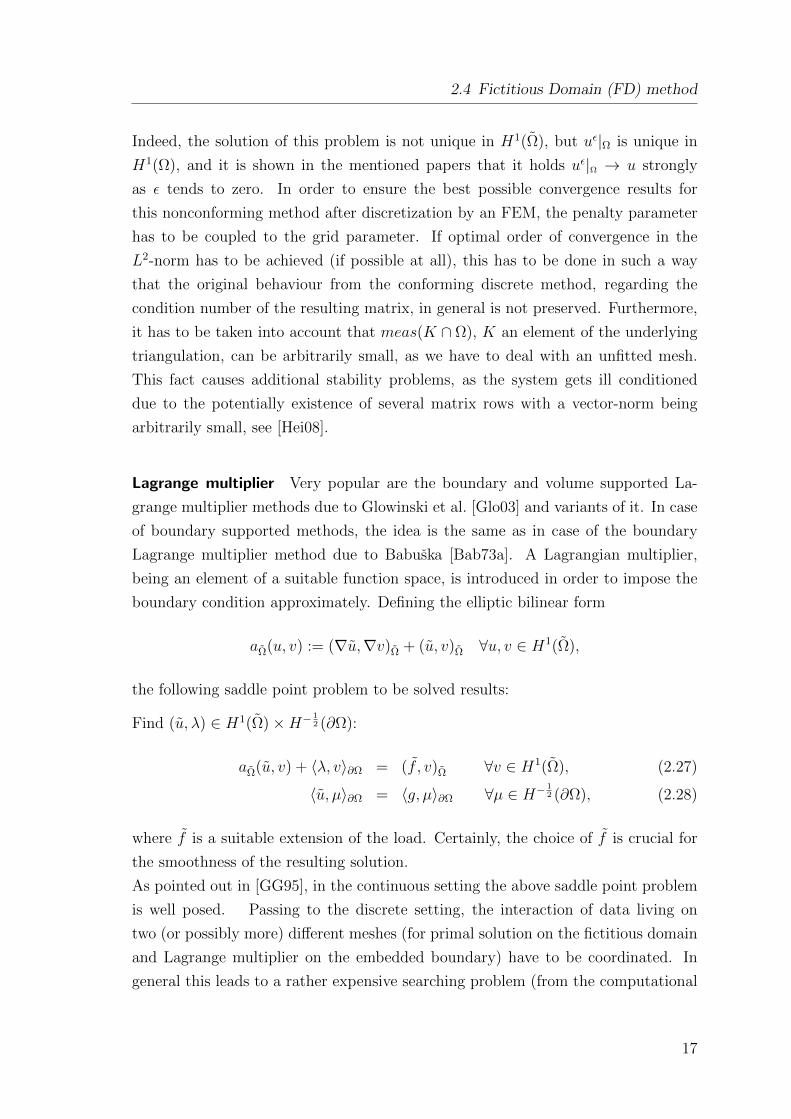
Indeed, the solution of this problem is not unique in H1(Ω), but uε|Ω is unique in
H1(Ω), and it is shown in the mentioned papers that it holds uε|Ω → u strongly
as ε tends to zero. In order to ensure the best possible convergence results for
this nonconforming method after discretization by an FEM, the penalty parameter
has to be coupled to the grid parameter. If optimal order of convergence in the
L2-norm has to be achieved (if possible at all), this has to be done in such a way
that the original behaviour from the conforming discrete method, regarding the
condition number of the resulting matrix, in general is not preserved. Furthermore,
it has to be taken into account that meas(K ∩ Ω), K an element of the underlying
triangulation, can be arbitrarily small, as we have to deal with an unfitted mesh.
This fact causes additional stability problems, as the system gets ill conditioned
due to the potentially existence of several matrix rows with a vector-norm being
arbitrarily small, see [Hei08].
Lagrange multiplier Very popular are the boundary and volume supported La-
grange multiplier methods due to Glowinski et al. [Glo03] and variants of it. In case
of boundary supported methods, the idea is the same as in case of the boundary
Lagrange multiplier method due to Babuska [Bab73a]. A Lagrangian multiplier,
being an element of a suitable function space, is introduced in order to impose the
boundary condition approximately. Defining the elliptic bilinear form
aΩ(u, v) := (∇u,∇v)Ω + (u, v)Ω ∀u, v ∈ H1(Ω),
the following saddle point problem to be solved results:
Find (u, λ) ∈ H1(Ω)×H− 12 (∂Ω):
aΩ(u, v) + 〈λ, v〉∂Ω = (f , v)Ω ∀v ∈ H1(Ω), (2.27)
〈u, µ〉∂Ω = 〈g, µ〉∂Ω ∀µ ∈ H−12 (∂Ω), (2.28)
where f is a suitable extension of the load. Certainly, the choice of f is crucial for
the smoothness of the resulting solution.
As pointed out in [GG95], in the continuous setting the above saddle point problem
is well posed. Passing to the discrete setting, the interaction of data living on
two (or possibly more) different meshes (for primal solution on the fictitious domain
and Lagrange multiplier on the embedded boundary) have to be coordinated. In
general this leads to a rather expensive searching problem (from the computational
17
2 Description of the model equations
point of view) when combining the data from the different grids. The boundary
grid parameter η > 0 has to be chosen carefully in order to get a discrete inf-sup
condition satisfied. In [GG95] a mixed FEM employing a P1/P0 pairing was studied,
and the compatibility condition
3h < η < Lh
has been deduced to make the discrete spaces compatible.
Different ways of avoiding such rather vague compatibility conditions and get the
resulting saddle point problem well posed are given e.g. in [HY09] and [BH10a].
In [HY09], inspired by XFEM methods (see below), the discrete inf-sup condition is
circumvented by a stabilization method in the spirit of Barbosa and Hughes [BH91].
Cut elements and stabilization are used in [BH10a].
In addition to the boundary Lagrange multiplier methods, having the drawback of
being not well suited in case of an a priori unknown evolution of Ω, the volume
based Lagrange multiplier methods have been developed, see e.g. [Glo03] and the
literature therein. The idea: Let ω ⊂ Ω be an open domain and Ω = Ω ∪ ω, extend
the resulting weak problem to Ω, and augment the formulation by a suitable scalar-
product over H1(ω) in order to get to an appropriate saddle point problem. Variants
of this methods have been widely used for simulation of incompressible viscous flow
around rigid bodies as well as fluid particle interaction, see e.g. [GPH+99,Bon06].
Variants of Nitsches method In [Nit71] Nitsche presented a method for imposing
the essential Dirichlet boundary conditions in a weak sense by applying the discrete
weak formulation:
Find uh ∈ Vh ⊂ H1(Ω) :
aΩ(uh, vh)− 〈∂nuh, vh〉∂Ω − 〈uh, ∂nvh〉∂Ω + 〈γDh−1uh, vh〉∂Ω
= (f, vh)Ω + 〈gD, γDh−1vh − ∂nvh〉∂Ω ∀vh ∈ Vh
for discretization of problem (2.23)-(2.24) within a discrete space of functions not
satisfying constraint (2.24) in case of a mesh fitted to the domain Ω by an FEM. An
extensive review on Nitsches method can be found in [Han05]. The parameter γD > 0
can in principle be estimated by solving an eigenvalue problem, see also [Han05].
This kind of penalty method turns out to be of optimal order in the H1- and
18

2.4 Fictitious Domain (FD) method
L2-sense, while maintaining the condition of the original discrete problem with
boundary conditions already incorporated into the discrete function space. Nitsches
method and its variants have been employed and studied extensively in the context
of different fields like fluid-structure interaction (e.g. [BF09, HH03]), optimization
(e.g. [Bec02,Duc10]), domain decomposition (e.g. [BHS01,Ste98]) and FD methods
(e.g. [CB09,BH10b]). It is directly related to a stabilized boundary Lagrange multi-
plier method on the one hand, and the boundary penalty method on the other hand,
see [JS08] and [Ste95]. In this work other regularized variants of Nitsches method
are given and analyzed in order to impose boundary conditions approximately in
the case of an unfitted mesh.
Immersed boundary Another popular family of methods are the so called Im-
mersed Boundary methods due to Peskin et al., see e.g. [Pes72,Pes02] and the liter-
ature therein. The key component is the imposition of the boundary conditions by
appropriate delta distributions, describing suitable punctual penalty forces on the
embedded inner boundary. As this kind of method is very popular in the context
of fluid-structure interaction, this forcing terms often are interpreted as and stem
from a feedback control of the physical forces acting on a structure. First order
accuracy can be granted in the original version, although higher order accuracy has
been reached, see for example [LP00].
Extended FEM (XFEM) In order to handle different kinds of discontinuities like
cracked and holed domains (e.g. [MDB99,SCMB01]), interface problems (e.g. [CB03,
GR07]) and later on in FD and related methods (e.g. [HY09, BBH10]), the XFEM
has been introduced. A basis is the partition of unity method due to Babuska et
al. [BM97]. The principle of the original extended FEM is the enrichment of a
standard continuous FE space with suitable local FE functions, while the set of the
enriched functions gives a partition of unity. The enriched space allows to handle
the physical forces/conditions in an adequate and more elegant way compared to
standard FE methods without complicated meshing. Existing discontinuities and
other troublemakers are resolved by means of the enriched function space.
19

2 Description of the model equations
Discontinuous Galerkin (DG) methods In [LB08] an example of an FE method,
using continuous elements on the part of the mesh not being intersected by the
boundary, and elementwise discontinuous functions on elements intersected by the
boundary, is proposed. In the interface zone, a geometry dependent local FE basis of
discontinuous functions, fulfilling zero boundary conditions exactly on the embedded
boundary described by a level set function is used. The method was analyzed
in [LN11] and turns out to be of almost optimal order.
Another approach using a set of discontinuous FE basis functions on the overall grid
meshing the fictitious domain is presented in [EB05]. In this method first the parts
of the domain lying within each element of the covering grid are detected, using a
two-dimensional bisection if necessary. The advantage of this method is that it can
handle very complex domains, but the bisection procedure is not a cheap one from
the computational point of view, and the shape of the artificial elements possibly
violates the cone condition.
Composite FE Originally created as an effective geometrical multigrid precondi-
tioner in the case of complicated domains, the composite FE method and its vari-
ants have been fully developed to handle boundary value problems like the Poisson
problem, and also the Stokes problem, in the case of arbitrarily mixed boundary
conditions, while the mesh does not resolve the geometrical details in a direct way,
see [HS97, Rec06, PS08, PS09]. A container-grid, covering the original domain, is
departed into standard degrees of freedom and the so called slave nodes, being as-
sociated to the degrees of freedom on elements cut by the domain boundary. On
the part of the mesh including the slave nodes, the essential and natural boundary
conditions are imposed approximately by extending the shape functions in the inner
part of the original domain under consideration, and projecting this extension in a
suitable way. So the shape of the finite element functions is adapted to fulfill the
boundary constraints in order to impose the boundary conditions.
20

2.4 Fictitious Domain (FD) method
2.4.2 Scalar problem with mixed boundary conditions
Now we will formulate a linear scalar model problem being closely related to a
linearized version of the (stationary) subproblems for the individual species treated
above. Due to this latter fact, and in order to demonstrate the principles of the
fictitious domain approach we will present here, we focus on the solution of
−∇ · (D∇u) + β · ∇u+ cu = f on Ω, (2.29)
u = gD on ΓD, (2.30)
D∂nu = gN on ΓN . (2.31)
It shall be pointed out, that there are different ways to linearize the non-linear
subproblems, but in almost every case this leads to a similar problem of solving an
equation like the given one.
In order to guarantee the unique solvability of this model problem, we make the
following assumptions on the equation data to bring the Lax-Milgram theorem into
play:
D, βi, c ∈ L∞(Ω); (2.32)
∃ θ > 0 : D ≥ θ a.e. in Ω; (2.33)
f ∈ L2(Ω); (2.34)
gD ∈ L2(ΓD); (2.35)
gN ∈ L2(ΓN); (2.36)
β · n ≥ 0 a.e. on ΓN ; (2.37)
∃ c0 > 0 : c− 1
2∇ · β ≥ c0 a.e. in Ω. (2.38)
The velocity field β = (βi)i=1,...,d and the rest of the data are supposed to be suffi-
ciently smooth to match these assumptions.
In [GPWZ96] and [GP92] a regularized/penalized fictitious domain method for linear
reaction-diffusion equations with Neumann boundary conditions was presented. We
will adapt the ideas presented in the mentioned papers to this more general problem
with a non-symmetric operator, including an additional convection term and mixed
boundary conditions. In order to do so, we embed the domain Ω into the larger
rectangular domain Ω, where Ω ⊂ Ω (see figure 2.2). Following Glowinski et al.
21
2 Description of the model equations
[GP92] let Ω be of class C0,1.
ΓD
ΓN
Ω
Ω
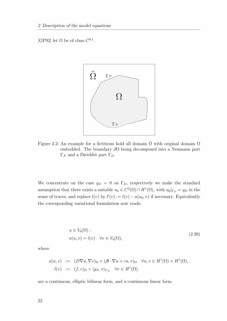
Figure 2.2: An example for a fictitious hold all domain Ω with original domain Ωembedded. The boundary ∂Ω being decomposed into a Neumann partΓN and a Dirichlet part ΓD.
We concentrate on the case gD = 0 on ΓD, respectively we make the standard
assumption that there exists a suitable u0 ∈ C2(Ω)∩H1(Ω), with u0|ΓD = gD in the
sense of traces, and replace l(v) by l′(v) := l(v)− a(u0, v) if necessary. Equivalently
the corresponding variational formulation now reads:
u ∈ V0(Ω) :
a(u, v) = l(v) ∀v ∈ V0(Ω),(2.39)
where
a(u, v) := (D∇u,∇v)Ω + (β · ∇u+ cu, v)Ω ∀u, v ∈ H1(Ω)×H1(Ω),
l(v) := (f, v)Ω + 〈gN , v〉ΓN ∀v ∈ H1(Ω).
are a continuous, elliptic bilinear form, and a continuous linear form.
22

2.4 Fictitious Domain (FD) method
Now let us define the following spaces/subsets:
V := H1(Ω) or V := H10 (Ω),
VΓD := v ∈ V : v|ΓD = 0 ,
H := v ∈ VΓD : a(v, µ) = l(µ) ∀µ ∈ VΓD ,
H0 := v ∈ VΓD : a(v, µ) = 0 ∀µ ∈ VΓD .
Note that
H1(Ω) = v : v = v|Ω, v ∈ V , (2.40)
V0(Ω) = v : v = v|Ω, v ∈ VΓD , (2.41)
i.e. H1(Ω) is embedded in V and V0(Ω) is embedded in VΓD . The assumption on Ω
to be of class C0,1 was used for this kind of embedding of the function spaces.
As the problem (2.39) under consideration has a unique solution due to the Lax-
Milgram theorem, the subsets H, H0 thus are non-empty closed convex subsets of
H1(Ω). It follows that the variational inequality
u ∈ H :
b(u, v − u) ≥ 0 ∀v ∈ H,(2.42)
where b : V × V → R is the continuous, V -elliptic bilinear form
b(v, w) := (∇v,∇w)Ω + α(v, w)Ω ∀v, w ∈ V, (2.43)
has a unique solution, see e.g. [LGT81]. Here α ≥ 0 is a constant, and α > 0 in case
of V = H1(Ω). We consider then the regularized problem
uρ ∈ VΓD :
ρb(uρ, v) + a(uρ, v) = l(v) ∀v ∈ VΓD .(2.44)
In this formulation the parameter ρ > 0 is a penalty/regularization parameter.
While the mentioned papers treat the case of a linear reaction-diffusion equation with
Neumann boundary conditions, in our case there are mixed boundary conditions
and an additional, probably dominant, convective term included as well. Thus, the
23

2 Description of the model equations
equations under consideration are not symmetric anymore, and hence this is true
for the corresponding bilinear forms, also.
An analysis of the proof of Theorem 3.1 in [GPWZ96] shows that the resulting
statement is still true in the considered case. So we get the following theorem:
Theorem 2.3. Let Ω ⊂ Rd (d = 2, 3) be a C0,1 domain and ρ > 0 a parameter. Let
u, u and uρ be the solutions of the problems (2.39), (2.42) and (2.44), respectively.
Then there holds:
limρ→0‖uρ − u‖H1(Ω) = 0,
limρ→0
ρ−12‖uρ − u‖H1(Ω) = 0. (2.45)
Proof. The proof closely follows the one from [GPWZ96], which is a typical conver-
gence proof for regularization problems. We will show the result in three steps.
(1) Boundedness of the family uρρ>0.
As there holds u|Ω = u and u|ΓD = 0 we get the relation
a(u, v) = l(v) ∀v ∈ VΓD . (2.46)
By taking v = uρ − u ∈ VΓD in (2.46) and by (2.44) we get
b(uρ − u, uρ − u) +1
ρa(uρ − u, uρ − u)
= −b(u, uρ − u) +1
ρl(uρ − u)− a(u, uρ − u) (2.47)
= −b(u, uρ − u).
From the latter relation, the continuity and ellipticity of b over V × V and the
ellipticity of a over V0(Ω)× V0(Ω) it follows:
C(‖uρ − u‖2
1,Ω+ ρ−1‖uρ − u‖2
1,Ω
)≤ ‖b‖‖u‖1,Ω‖u
ρ − u‖1,Ω ∀ρ > 0, (2.48)
where C > 0 is an appropriate constant. This implies the boundedness
‖uρ‖1,Ω ≤ C ∀ρ > 0, (2.49)
as u is fixed.
24
2.4 Fictitious Domain (FD) method
(2) Weak convergence of the family uρρ>0.
From the boundedness of uρρ>0 there exists a subsequence uρkρk>0, such that
limρk→0
uρk = u∗ (2.50)
weakly in H1(Ω). Hence by taking the limit ρk → 0 in (2.44) we obtain:
a(u∗, v) = l(v) ∀v ∈ VΓD ,
and thus we have
u∗ ∈ H. (2.51)
Taking into account that v|Ω = u and v|ΓD = 0 ∀v ∈ H we get:
a(v, v − uρ) = l(v − uρ) ∀v ∈ H. (2.52)
After replacing v by v − uρ ∈ VΓD in (2.44), using the V0(Ω)-ellipticity of a and
combining with the latter relation, we obtain (setting ρk = ρ)
b(uρ, v) = b(uρ, uρ) +1
ρ−a(uρ, v − uρ) + l(v − uρ)
≥ b(uρ, uρ) +1
ρ−a(v − uρ, v − uρ)− a(uρ, v − uρ) + l(v − uρ)
= b(uρ, uρ) +1
ρ−a(v, v − uρ) + l(v − uρ) (2.53)
= b(uρ, uρ) ∀v ∈ H.
Combining this result with the continuity and ellipticity properties of b we have:
b(u∗, v) ≥ b(u∗, u∗) ∀v ∈ H. (2.54)
Hence u∗ is a solution of problem (2.42). As problem (2.42) has a unique solution
u, the weak convergence of the whole family to u follows.
(3) Strong convergence of the family uρρ>0.
From equation (2.47), using the ellipticity properties of the bilinear forms under
consideration, the weak convergence of the family uρρ>0 to u and that there holds
25

2 Description of the model equations
u|Ω = u we obtain:
limρ→0
(‖uρ − u‖2
1,Ω+
1
ρ‖uρ − u‖2
1,Ω
)= 0.
Which implies the desired result.
An analysis of the last proof shows that the bilinear form a and linear form l only
have to fulfill the standard assumptions regarding coercivity and continuity. So
other linear forms standing in context to the model problem, or problems close to
it, are included within the statement of an analogous theorem as well.
In the case of a pure Neumann problem, or by substituting the essential Dirichlet
conditions, or both of the given boundary conditions, by Robin conditions, there
would be no need to incorporate the corresponding boundary constraints into the
underlying function space. The latter would be necessary when providing the penalty
problem to a numerical method, in order to get an advantage over a standard method
in case the mesh can or is not fitted to the inner boundary. As a consequence, the
method is not intended for direct usage.
The real advantage, as will be shown later on, is the combination with Nitsches
method (see [Nit71]) in order to impose the essential boundary condition accurately
in a weak sense. Other methods based on a kind of boundary penalty, see e.g. [BE86]
and [Bab73b], would fit into the context, too.
One word on pure Neumann problems: The mixed case is set back to the original
one handled in the mentioned papers by simply setting ΓD = ∅ and substituting
VΓD by V .
2.4.3 Fictitious Domain Oseen problem
After providing the theoretical background for a fictitious domain method in case
of a scalar model problem, the same thing will be done with the help of a model
problem being close to linearized versions of the stationary Navier-Stokes equations
in the vector valued case. For ease of presentation we keep the focus on homogeneous
Dirichlet conditions on the whole boundary, but the case of Neumann conditions also
included is not far away.
26
2.4 Fictitious Domain (FD) method
A vector valued model problem, well suited for this goal, is the Oseen problem with
sufficiently smooth data analogously to the scalar case:
−∇ · (ν∇u) + (β · ∇)u+ σu+∇p = f in Ω (2.55)
∇ · u = 0 in Ω (2.56)
u = 0 on ΓD. (2.57)
As already done in the case of the Stokes problem above, in this theoretical part we
give the weak formulation using divergence-free spaces and keeping the notation of
paragraph 2.3.2:
u ∈ V0,div(Ω) : A(u,v) = (f ,v)Ω ∀v ∈ V0,div(Ω), (2.58)
where
A(u,v) := Bdiv(u,v) + ((β · ∇)u,v)Ω + (σu,v)Ω ∀u,v ∈(H1(Ω)
)d. (2.59)
Clearly, it is possible to generalize the theoretical framework of the scalar case using
the underlying function spaces, as each of the components of this system is of the
form (2.29)-(2.30). Hence the regularized/penalized problem prepared for handling
the original problem on a suitable fictitious domain Ω reads:
uρ ∈ VΓD,div : ρ(∇uρ,∇v)Ω + A(uρ,v) = (f ,v)Ω ∀v ∈ VΓD,div, (2.60)
where in this case
VΓD,div :=
v ∈
(H1(Ω)
)d: v|ΓD = 0, ∇ · v = 0 a.e.
,
and ρ > 0 again is a penalty parameter.
27

2 Description of the model equations
2.5 Description of domain geometries
A survey and comparison on suitable methods for describing geometries in flow
problems, applicable for a wider class of problems also, is given e.g. in [Jim04]. As
always let Ω ⊂ Rd be a domain with sufficiently smooth boundary Γ = ∂Ω, and
Ω ⊂ Rd, with Ω ⊂ Ω, be a covering domain. One way of treating the boundary of
an embedded complex or time dependent domain is to interpret the boundary as a
front between two different chemical/physical species, while only the behaviour of
one species (the one contained in Ω) is of relevance for the original problem. Two
general concepts of describing complex or time dependent domains in this sense can
be distinguished:
• Front tracking methods, describing the boundary/interface Γ as the boundary
of a (in general) time-dependent subdomain explicitly, using a boundary-fitted
mesh for numerical methods.
• Front capturing methods, describing the underlying geometry in an implicit
way on a fixed covering domain Ω, without a boundary-fitted grid on the
resulting discrete level.
We will concentrate on the second concept, being a kind of Eulerian framework,
in order to describe the underlying geometry in an implicit way by a scalar field
φ : Ω × I → R, where as always I is a time interval. We will now discuss popular
and common ways of describing a co-dimension one surface implicitly, needed for
our purpose.
The transport equation
∂tφ+ v · ∇φ = 0 on Ω× (0, T ], (2.61)
φ(x, 0) = φ0(x) on Ω, (2.62)
in many cases plays a key role in order to get the scalar field, for it can be interpreted
as describing the evolution of the zero level set of a function φ in time with respect
to a given (or estimated) velocity field v.
28

2.5 Description of domain geometries
Phase Field Method One kind of implicit description utilizes the so called phase
field function φ, see for example [EGK08], which covers the boundary of the domain
Ω, being the surface or curve to describe, in a diffusive sense. Depending on whether
the function value is one or zero in a given point, this point is within or out of
Ω. Moreover, the interface-zone, covering Γ, has typically the form of a tube of
maximal-width ε > 0. In this zone φ behaves like a regularized step-function. The
parameter ε typically is proportional to the grid width of a covering triangulation
on the numerical level. The phase field function can be calculated by solving the
Cahn-Hillard equation, be constructed from a signed distance function, for example
after solving the transport equation (2.61)-(2.62), or from external data. This kind
of description is well suited if the boundary has to be smeared out, see [Jim04].
Volume of Fluid Another common way of implicit description, somewhat akin to
the phase field method, often used in multi-physical interface problems of fluids, is
the volume of fluid method, see [HN81]. φ is a (ideally) cellwise constant function,
where φ(x, t) ∈ [0, 1] gives the volume fraction of the fluids and thus provides a way
of giving information regarding the position with respect to the domain Ω and Ω\Ω,
both filled by different fluids. Again an equation of the form (2.61)-(2.62) often is
employed in order to get a suitable scalar field φ.
Level Set Method The way of implicit description chosen in this work is the so
called level set framework, see e.g. [Set99] and [OS88]. A level set function is a
(smooth) scalar field φ : Ω × (0, T ] → R, which is often calculated from the first
order hyperbolic transport equation (2.61)-(2.62).
Ideally the level set function is a signed distance function, that is it holds ‖∇φ‖ = 1.
This is for reason of mass conservation, see [Set99, SFSO97], and for a good and
geometrically intuitive description of the co-dimension one surface either, because
as the name already says, the function just gives the signed distance of a point
in x ∈ Rd to the surface; the sign depends on the local orientation of the latter.
It allows for the construction of an oriented normal vector field, needed in various
calculations in an adequate and easy way as well. Moreover, a sharp description of
the boundary can be obtained.
29

2 Description of the model equations
φ > 0
φ < 0
n = ∇φ|Γ
Figure 2.3: Example of the implicit description of a circle Br(xm, ym) within acovering domain Ω. The level set function in this case is given byφ(x, y) :=
√(x− xm)2 + (y − ym)2 − r.
The implicit description of Ω embedded in a larger domain Ω ⊂ Ω is very intuitive
and works like that:
φ(x) < 0 if x ∈ Ω,
φ(x) = 0 if x ∈ ∂Ω,
φ(x) > 0 if x ∈ Ω \ Ω.
So a simple evaluation of φ gives information regarding the surface at time t, see
Figure 2.3.
30

3 Discretization
In this chapter the discretization of the coupled systems of equations from Chapter
2 will be described. More precise, we will deal with appropriate linear prototypes,
being closely related to linearizations of the original systems of equations from Sec-
tion 2.2 and 2.3. We will focus on the two-dimensional case, but the methods can
be extended to the three-dimensional case as well.
As we potentially have to handle complex and time-dependent domains, and we do
not want to employ a re-meshing algorithm, which may produce a very poor grid (see
for discussion within the previous chapter), we will use a fictitious domain method.
In order to respond to these goal we focus on numerical aspects like stability and
the weak incorporation of boundary conditions on implicitly given domains.
We start by formulating assumptions on the relation between covering grid and
domain Ω in general. Next an adequate discrete weak formulation of the linear
model problems, using the penalty/regularized/FD framework already described in
Chapter 2, is developed. This is done for scalar model problems first, followed by
another related one for an Oseen model problem. After that we deal with accurate
techniques of semi-discretization in time in case of non stationary problems.
In general the model equations and the non-linear RDC-Systems will be convec-
tion dominated. So we will have to take care about choosing a robust numerical
scheme, being able to handle the resulting problems due to stability and spurious
non-physical oscillations, while fitting into the overall framework at the same time.
The discretization of the Stokes and Navier-Stokes systems, based on the Oseen
model problem stated below, is given similar to the scalar model equations, but under
the additional aspect of the pressure, to be understood as a Lagrangian parameter
to ensure the incompressibility condition. Thus, a discrete saddle point problem
has to be solved, using Galerkin least squares stabilization techniques to circumvent
a discrete inf-sup condition, which is not fulfilled in case of the FE spaces defined
below.
31
3 Discretization
While in the standard case a polygonal boundary is given which is part of the closure
of a triangulation, we will have to deal with an only implicitly given boundary
which cuts an unfitted mesh (see also [BH10a, BH10b] for example). Thus, we will
employ the utilities from Section 2.4.2. Whereas in the latter the incorporation of
Dirichlet boundary conditions is an essential part of the considered function spaces,
we will describe this conditions in an adequate weak sense using Nitsches method,
see [Nit71].
3.1 Assumptions on domain and triangulation
Let Ω be a suitable rectangular domain in R2, see Section 2.4.2, with Ω ⊂ Ω. We
will make the additional assumption on Ω to be of class C2, which makes it possible,
among other things, to define the boundary of the domain by a locally smooth level
set function being a signed distance function (see [LN11] and the literature therein).
Furthermore, the following assumptions and definitions regarding the domain Ω, its
boundary Γ and the triangulations of the fictitious domain Ω are made:
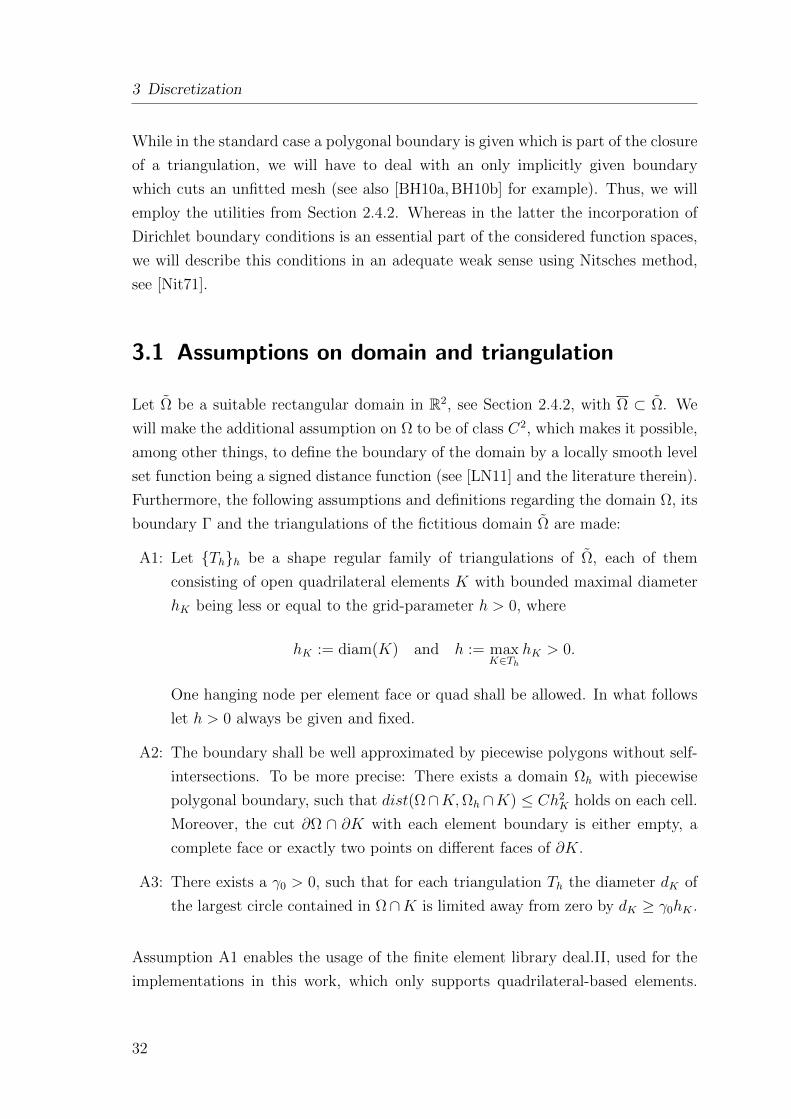
A1: Let Thh be a shape regular family of triangulations of Ω, each of them
consisting of open quadrilateral elements K with bounded maximal diameter
hK being less or equal to the grid-parameter h > 0, where
hK := diam(K) and h := maxK∈Th
hK > 0.
One hanging node per element face or quad shall be allowed. In what follows
let h > 0 always be given and fixed.
A2: The boundary shall be well approximated by piecewise polygons without self-
intersections. To be more precise: There exists a domain Ωh with piecewise
polygonal boundary, such that dist(Ω∩K,Ωh ∩K) ≤ Ch2K holds on each cell.
Moreover, the cut ∂Ω ∩ ∂K with each element boundary is either empty, a
complete face or exactly two points on different faces of ∂K.
A3: There exists a γ0 > 0, such that for each triangulation Th the diameter dK of
the largest circle contained in Ω∩K is limited away from zero by dK ≥ γ0hK .
Assumption A1 enables the usage of the finite element library deal.II, used for the
implementations in this work, which only supports quadrilateral-based elements.
32

3.1 Assumptions on domain and triangulation
The hanging nodes give rise for efficient and easy to implement local refinement
algorithms. In the case of continuous FE the additional constraints to be fulfilled
on a side shared by three elements is ensured by elimination/condensation before
solving the resulting system, see [BHK].
Assumption A2 represents the wish for the boundary of the domain to be resolved
sufficiently good enough by the underlying mesh in some sense, as well as to use
an adequate polygonal approximation of it in the concrete implementation, see Sec-
tion 4.1. If necessary it would be possible to reach this state by local refinements
and/or local geometrical smoothing. The methods under consideration thus treats
boundaries without self-intersection and local protuberances with respect to the grid.
Moreover, the boundary should be sufficiently smooth. Methods better suited for
the direct treatment of complex rough boundaries, like the composite FE method,
are discussed in Subsection 2.4.1.
In [DBDV10] a domain and the underlying grid are called compatible, if a slight
variation of Assumption A3 is valid. This clearly is well founded, as with A1-
A3 being valid, the following proposition, being a variant of Proposition 4.1 in
[DBDV10], can be given, bringing the roundedness of a local element K ∩Ω in case
meas(K ∩ Ω) > 0 into play (see also the discussion in the next section).
Proposition 3.1. Let Assumptions A1-A3 be true in case of Ω, with Ω ⊂ Ω and
the triangulation Th of Ω. Let (K,P,Σ) be an associated finite element and k,m
nonnegative integers such that m < k. Assume that Π ∈ L(Hk+1(K), P ) is a bounded
projection and P ⊂ Hm(K∩Ω), where P is a polynomial finite dimensional subspace.
Then there exists a constant C > 0, not depending on u ∈ Hk+1(K) and h, such
that
|u− Πu|m,K∩Ω ≤ Chk+1−m|u|k+1,K∩Ω. (3.1)
Proof. Due to the assumed kind of shape regularity, the standard techniques of
interpolation theory, based on the Bramble-Hilbert lemma, can be utilized in order
to get the result.
The last proposition now opens the gate for analyzing FEMs in the context of the
purposed FD methods. Moreover, Assumption A3 will be a key to the error analysis
in the next two sections.
33

3 Discretization
3.2 FD discretization for the scalar model equation
The regularized/penalized fictitious domain method of Section 2.4.2, based on the
ideas of [GP92] and [GPWZ96] for the model equation (2.29)-(2.31), is now adapted
to variants of Nitsches method, see [Nit71]. The reason for doing so is the ability of
this methods to impose the essential Dirichlet boundary conditions accurately in a
weak sense. In the original formulation of Section 2.4.2 adjusted function spaces for
considering the Dirichlet boundary conditions have been used. As the boundary is
given only implicitly and the mesh will in general not be fitted to Γ, those spaces
are not available. Thus, Nitsches method is an accurate way for imposing essential
boundary conditions in a weak sense, when passing over to a discretization of the
model equations or the non-linear RDC system.
In what follows let C > 0 always be a generic constant if not stated otherwise. Let
ΓD,K := ΓD ∩K and ΓN,K := ΓN ∩K,
if K∩Γ 6= ∅. We will describe and analyze the methods at hand under the premise of
the absence of variational crimes in the form of approximating a smooth boundary by
an appropriate polygonal set, which in fact is done in the concrete implementation.
For the details on that see Section 4.2. Using the finite-dimensional space
Vh = v ∈ C0(Ω)
: v|K ∈ Q1(K) ∀K ∈ Th, v = 0 on ∂Ω ⊂ H10 (Ω)
of picewise bilinear elements, the discrete weak formulation can be stated as:
Find uρh ∈ Vh such that
a∓h (uρh, vh) + ρb(uρh, vh) = l∓h (vh) (3.2)
for all vh ∈ Vh and ρ > 0. The discrete bilinear forms a∓h (·, ·), b(·, ·) respectively the
linear form l∓h (·) are defined as:
a∓h (u, v) := a(u, v)− 〈D∂nu, v〉ΓD ∓ 〈Du, ∂nv〉ΓD +
+∑ΓD,K
γ∓DhK〈Du, v〉ΓD,K − 〈(β · n)−u, v〉ΓD ,
34

3.2 FD discretization for the scalar model equation
b(u, v) := (∇u,∇v)Ω,
l∓h (v) := l(v)∓ 〈DgD, ∂nv〉ΓD +∑ΓD,K
γ∓DhK〈DgD, v〉ΓD,K
−〈(β · n)−gD, v〉ΓD + 〈gN , v〉ΓN ,
where γ∓D > 0 is a stabilization parameter, being a sufficiently large real number.
In what follows we often refer to those two different FE formulations as (3.2)− and
(3.2)+. Furthermore, let
(y)− :=
y if y < 0,
0 else,
and
(y)+ :=
y if y > 0,
0 else.
Before coming to the proof of the well-posedness of the two discrete problems (3.2)∓,
a short briefing on the terms appearing in this formulation is given, see also [JS08]:
• The first boundary integral in the definition of a∓h (·, ·) stems from testing the
model PDE and integrating by parts, splitting the boundary into ΓD and ΓN .
• The third term in the definition of a∓h (·, ·) is added in order to preserve symme-
try in H1(Ω) in case the minus is chosen, while else with the plus the resulting
method has better stability properties, see next subsection.
• In general choosing the symmetry preserving version (3.2)− results in a more
accurate method, at least in case of boundary fitted shape regular meshes,
see [ABCM02]. But the latter has drawbacks when using unfitted meshes,
which will be discussed later on.
• The sum over the cellwise parts of ΓD is added for stability reason, as well as
the last term, which allows a better control of the convection term, see [RST08].
• In all cases a counterpart on the right hand side is added in order to guarantee
consistency, taking into account the boundary conditions of the model problem
in strong formulation.
35

3 Discretization
So far so classical, but in order to assure stability, care has to be taken when dealing
with the roundedness of a local element K ∩ Ω next to ΓD, similar to the case of
the original Nitsche method, see [Han05]. For demonstration a cellwise constant
parameter hΓD,K is defined, giving a measure of shape regularity of the involved
implicitly given elements Ω ∩K in case of K ∩ ΓD 6= ∅:
hΓD,K :=
hK if three nodes are in K ∩ Ω,
min(hK,1, hK,2) if two nodes are in K ∩ Ω,
min(hK,1, hK,2) if one node is in K ∩ Ω,
(3.3)
where hK,1, hK,2 > 0 are the Euclidean distances between the two intersections
∂Ω ∩ ∂K and the in each case closest vertex inside Ω, see Figure 3.1.
hΓD,K = hK,2
K ∩ Ω
ΓD,K
hK,1
hK,2
K ∩ Ω
ΓD,K
hK,1hK,2
hΓD,K = hK,1
ΓD,K
K ∩ Ω
hK
hΓD,K = hK
Figure 3.1: The pictures visualize the definition of the parameter hΓD,K . In the leftsituation it is hΓD,K = hK,2, while in the middle we set hΓD,K = hK,1. Inthe right picture hΓD,K can be set to the cell-diameter.
Especially the definition of the second and the last case in (3.3) depends on the
existence of a minimal diameter dK > 0 of a circle completely within the local cut
K ∩Ω, as pointed out in [Han05] and [BH10b] as well. While this is obvious for the
third case, in the second case this is due to the fact that the local cut with the mesh
has the form of a (deformed) rectangle (small sliver cut). Even if meas(ΓD,K) has
a finite value, meas(K ∩ Ω) does not have to be bounded away from zero, causing
hΓD,K to tend to zero.
However, providing Assumption A3 holds, there will be a constant γK ∈ (0, 1] with
hΓD,K = γKhK and a circle with diameter hΓD,K/2 = γKhK/2 ≥ γ0hK bounded away
from zero.
In order to analyze the method we will need the following versions of trace/inverse
inequalities.
36

3.2 FD discretization for the scalar model equation
Proposition 3.2. Let Assumptions A1-A3 be true. Then there holds
h12K‖v‖0,ΓK ≤ C(‖v‖0,K∩Ω + hK |v|1,K) ∀v ∈ H1(K), (3.4)
h12K‖∂nv‖0,ΓK ≤ C(|v|1,K∩Ω + hK |v|2,K) ∀v ∈ H2(K), (3.5)
h12K‖∂nvh‖0,ΓK ≤ C‖∇vh‖0,K∩Ω ∀vh ∈ Vh, (3.6)
with a bounded constant C > 0 and ΓK := Γ ∩K.
Proof. These inequalities follow by using the trace Theorem (2.1) from [Bra03],
and a scaling argument. In more detail, and similar to the proof of Lemma 4.1
in [DBDV10]:
Let v ∈ H1(K), K := (0, 1)2, ϕK : K → K be the corresponding affine-linear
mapping and v := v ϕK ∈ H1(K). Due to the made assumptions ϕK(K ∩Ω) ⊂ K
is a Lipschitz domain. According to that we find:∫Γ∩K
v2 dΓ ≤∫
K∩ϕK(∂Ω)
v2 |JϕK | dΓ ≤ ‖v‖20,∂(ϕK(K∩Ω)) ≤ CK‖v‖2
1,ϕK(K∩Ω),
where CK is the Lipschitz constant of the local cut geometry, depending heavily on
the assumed roundedness of K ∩ Ω. Writing out the definitions of the norms and
by scaling we get
‖v‖20,Γ∩K ≤ CK
(‖v‖2
0,ϕK(K∩Ω) + |v|21,ϕK(K∩Ω)
)≤ CK
(h−1K ‖v‖
20,K∩Ω + hK |v|21,K∩Ω
)from which the the inequalities (3.4) and (3.5) follow again by using the assumed
roundedness by setting C := maxCK : K ∈ Th, K ∩ Γ 6= ∅. Taking into account
the norm-equivalence on finite-dimensional spaces inequality (3.6) follows, too.
Remark 3.1. Note that as Assumption A3 does not hold for every pair of triangu-
lation and embedded domain, the constant C from the last statement does not have
to be moderate or even is not bounded as γ0 does not have to be bounded away from
zero in general. In order to get around this problem, a slight additional geometrical
regularization might be necessary to ensure a minimal roundedness of the K ∩Ω in
any case, see Section 4.2 for a possible strategy.
37

3 Discretization
3.2.1 Stability of the discrete form
In order to make things clear, the case of a convection dominated problem, i.e. |D| |β|, is omitted for the moment. For ease of presentation the diffusion coefficient is
supposed to be constant within this section. The presentation is similar to the
analogous in the standard case, see e.g. [RST08].
Lemma 3.1. Assuming A1-A3 and (2.32)-(2.38) hold, for all vh ∈ Vh the bilinear
form ρb(·, ·) + a∓h (·, ·) satisfies
ρb(vh, vh) + a∓h (vh, vh) ≥ Cρ‖∇vh‖2
0,Ω+D‖∇vh‖2
0,Ω + c0‖vh‖20,Ω +
+ ‖|n · β|12vh‖2
0,ΓD+∑ΓD,K
D
hK‖vh‖2
0,ΓD,K
, (3.7)
with sufficiently large γ∓D ≥ γ0 > 0 and C > 0 being independent of h, ρ and u.
Proof. By the identity
1
2〈(n ·β), v2〉ΓD +
1
2〈(n ·β), v2〉ΓN =
1
2(∇ · (βv2), 1)Ω =
1
2(∇ ·β, v2)Ω + (β · ∇v, v)Ω,
being valid for all v ∈ H1(Ω) (H1(Ω) is embedded in this larger space), we find:
(β · ∇vh + cvh, vh)Ω − 〈(n · β)−vh, vh〉ΓD =
(c− 1
2∇ · β︸ ︷︷ ︸≥c0
, v2h)Ω + 1
2〈(n · β), v2
h〉ΓD + 12〈(n · β)︸ ︷︷ ︸≥0
, v2h〉ΓN − 〈(n · β)−vh, vh〉ΓD ≥
c0‖vh‖20,Ω + 1
2〈|n · β|, v2
h〉ΓD = c0‖vh‖20,Ω + 1
2‖|n · β| 12vh‖2
0,ΓD.
Consider now the terms 2D〈∂nvh, vh〉ΓD,K appearing in case a−h (·, ·) is chosen. We
find by applying the Cauchy-Schwarz and Young’s inequality, using inequality (3.6)
|2D〈∂nvh, vh〉ΓD,K | ≤ 2DCh− 1
2K ‖∇vh‖0,K∩Ω‖vh‖0,ΓD,K
≤ D
2‖∇vh‖2
0,K∩Ω +2DC2
hK‖vh‖2
0,ΓD,K.
Hence summation over all elements lying within Ω or including the artificial edges
38

3.2 FD discretization for the scalar model equation
ΓD,K yields:
ρb(vh, vh) + a−h (vh, vh) = ρ‖∇vh‖20,Ω
+D‖∇vh‖20,Ω + (β · ∇vh + cvh, vh)Ω +
− 2D〈∂nvh, vh〉ΓD +∑ΓD,K
Dγ−DhK‖vh‖2
0,ΓD,K− 〈(n · β)−vh, vh〉ΓD
≥ ρ‖∇vh‖20,Ω
+D
2‖∇vh‖2
0,Ω + c0‖vh‖20,Ω
+∑ΓD,K
D(γ−DhK− 2C2
hK)‖vh‖2
0,ΓD,K+
1
2‖|n · β|
12vh‖2
0,ΓD
for each function vh ∈ Vh.
After all coercivity of the discrete bilinear form b(·, ·) + a−h (·, ·) is ensured by the
choice γ−D ≥ γ0 ≥ 12
+ 2C2, where C from Proposition 3.2.
In case a+h (·, ·) is employed, simply setting γ+
D > 0 suffices, as the boundary terms
containing the normal derivatives erase each other.
It follows that problem (3.2) is well posed. Note that by choosing a+h (·, ·) in place
of a−h (·, ·) ones is far less dependent on Assumption A3 regarding the roundedness
of the local cut K ∩ Ω next to ΓD.
Another relation, taking effectively the place of the Galerkin orthogonality in this
case, see also [GP92], and will be used frequently in this work, comes from the
following lemma. The value of the penalty parameter ρ > 0 may change in different
situations.
Lemma 3.2. Let u ∈ H2(Ω) be the solution of the model problem (2.39), uρh is the
solution of the regularized discrete problem (3.2), then
a∓h (E2u− uρh, vh) = ρb(uρh, vh) ∀vh ∈ Vh. (3.8)
Proof. Due to the consistency arguments in the former paragraph (for further details
see e.g. [JS08]), using (2.29)-(2.31), and the properties of the extension operator we
can write
a∓h (E2u, vh) = l∓h (vh) ∀vh ∈ Vh,
using the fact that H1(Ω) is embedded in H10 (Ω). Substracting from this equation
(3.2) yields the relation.
39
3 Discretization
3.2.2 Stabilization in the convection dominated case
In order to give an analysis in case of a convection dominated problem, and for ease
of presentation, the diffusion coefficient in (2.39) is assumed to be a constant value
ε, being small compared to the norm of β at least in some part of the underlying
domain. It is well known, see for example [Joh90], that the discretization scheme
resulting from the standard Galerkin method gets unstable in case a dominating
convective term is added to the symmetrical part of the equation.
This is due to the weak ellipticity of the problem, with respect to its resulting ε-
weighted natural norm. In the numerical solution after lauching an FEM based on
standard Galerkin, non-physical oscillations can be observed in many cases.
Besides of these nonphysical features, this is a cause of trouble, especially when
the numerical solutions are of temporal nature, needed during an overall solution
process. The poor quality can lead to a breakdown of the superior task.
In order to stabilize a scheme, which often may have to treat with a dominating
convective part for the problems we have to deal with, a standard procedure is the
addition of consistency preserving terms (with respect to the original problem) of
the form ∑K∈Th
δK(Lu− f, ψ(u))Ω∩K ,
see e.g. [RST08]. The mesh dependent parameters δK > 0 will be chosen in a suitable
manner in order to ensure stability of the resulting scheme, covering the cases of a
reaction, diffusion or convection dominated problem, as will be shown later on.
Typical choices for ψ can be ψ(v) = β · ∇v (streamline diffusion, SD) or ψ(v) = Lv
(Galerkin least squares, GLS), with L being the underlying linear operator, or an
operator close to it. Other choices would be possible, depending on the nature of
the underlying problem. We will concentrate on the case ψ(v) = β · ∇v, that is
the streamline diffusion method. However, the basic principles stay the same for
many stabilization methods of this kind and thus the analysis further down can be
extended analogously.
The stabilized discrete weak formulation using the SD method with penalty param-
eter ρ > 0 now writes: Find uρh ∈ Vh, such that
A∓h (uρh, vh) + ρb(uρh, vh) = F∓h (vh) ∀vh ∈ Vh, (3.9)
40
3.2 FD discretization for the scalar model equation
where the linear forms are given by
A∓h (u, v) := a∓h (u, v) +∑K∈Th
δK(−ε4u+ β · ∇u+ cu,β · ∇v)Ω∩K ,
F∓h (v) := l∓h (v) +∑K∈Th
δK(f,β · ∇v)Ω∩K ,
defined for all u, v ∈ H1(Ω).
Note that due to the local consistency on Ω there holds
A∓h (E2u− uρh, vh) = ρb(uρh, vh) ∀vh ∈ Vh (3.10)
by the same argument used in the case of the non-stabilized method.
Lemma 3.3. Suppose the assumptions of Lemma 3.1 hold true. Let δK be an ele-
mentwise constant function satisfying
0 < δK ≤c0
c2K
, where cK := ‖c‖∞,K∩Ω,
on K ∩ Ω 6= ∅. Then the discrete bilinear form A∓h (·, ·) + ρb(·, ·) satisfies
A∓h (vh, vh) + ρb(vh, vh) ≥ Cρ‖∇vh‖2
0,Ω+ ε‖∇vh‖2
0,Ω + c0‖vh‖20,Ω +
+ ‖|n · β|12vh‖2
0,ΓD+∑K∩Ω
δK‖β · ∇vh‖2K∩Ω + (3.11)
+∑ΓD,K
D
hK‖vh‖2
0,ΓD,K
,
with sufficiently large γD ≥ γ0 > 0 and C > 0 being independent of h.
Proof. Due to (3.7) we only have to focus on the additional stabilization part. For
each function vh ∈ Vh there holds:∑K
δK(−ε4vh︸︷︷︸=0
+β · ∇vh + cvh,β · ∇vh)K∩Ω =
∑K∩Ω
δK(cvh,β · ∇vh)K∩Ω +∑K∩Ω
δK‖β · ∇vh‖2K∩Ω. (3.12)
Note that contributions from Laplacians are canceled out, as we effectively use
bilinear finite elements on Cartesian grids. We will give an upper bound for the
41

3 Discretization
absolute value of the first term resulting from stabilization, using the given constraint
on the parameter δK on each element/subelement.∣∣∣∣∣∑K∩Ω
δK(cvh,β · ∇vh)K∩Ω
∣∣∣∣∣ ≤ ∑K∩Ω
[δKc2K
2‖vh‖2
0,K∩Ω +δK2‖β · ∇vh‖2
K∩Ω
]≤
∑K∩Ω
[c0
2‖vh‖2
0,K∩Ω +δK2‖β · ∇vh‖2
K∩Ω
]≤ c0
2‖vh‖2
0,Ω +∑K∩Ω
δK2‖β · ∇vh‖2
K∩Ω.
This upper bound together with (3.7) yields the statement.
As can be seen from the statement of the last lemma, the SD adds artificial diffusion
in streamline direction resulting in a more of stability. But there still can be observed
over- and undershots in the finite element solution in the presence of sharp layers.
Thus, it can be necessary to augment the formulation by suitable shock capturing
stabilization terms, in order to add a good amount of artificial diffusion not only in
streamline direction. All this is due to the fact that the SD method does not satisfy
a discrete maximum principle by itself, which is not addressed in more detail in this
work.
Following [RST08], an alternative stabilized method for numerical solution of the
regularized/penalized problem, using additional local consistency preserving shock-
capturing terms, writes:
uρh ∈ Vh : ρb(uρh, vh) + A∓h (uρh, vh) + asc(uρh; vh) = Fh(vh) ∀vh ∈ Vh. (3.13)
As an example in this formulation the new terms are defined to be of the form
asc(u; v) :=∑
K∩Ω6=∅
(τK(u)∇u,∇v)K∩Ω,
τK(u) := τ ∗(R∗K(u)),
R∗K(u) :=‖Lu− f‖0,K
κK + ‖u‖1,K
,
where κK is a regularization parameter to ensure the well-posedness of the underlying
non-linear problem. τ ∗K = O(hγK) has to be chosen in such a way, that the order
of convergence of the overall scheme is preserved. Note that the consistency with
respect to the original problem is still preserved and thus the method fits into the
42

3.2 FD discretization for the scalar model equation
overall FD framework.
3.2.3 A priori error in the symmetric case
The symmetric case, i.e. β = 0 in (2.29), is treated first and separately, as it is the
easier one and as it is a special case often needed in applications as well.
As there will be given an a priori error bound for the error u − uρh in a suitable
norm, controlling both the L2(Ω)- and H1(Ω)-norms of the latter, later on, we first
want to give the result of Glowinski et al. from [GP92] for the case of ΓD = ∅ and
β = 0. Note that VΓD has to be replaced by V when using the nomenclature of
Section 2.4.2, as ΓD = ∅.
Clearly, assuming Ω is a C1,1 domain in Rd (d = 2, 3), f ∈ H2(Ω), g ∈ H12 (Γ),
the solution u of problem (2.29)/(2.31) in the considered case will be an element of
H2(Ω).
Theorem 3.1 (see [GP92]).
Let Ω ⊂ Rd (d = 2, 3) be a bounded Ck,1 domain, where k > max0, d/2 − 1 and
Ω ⊂ Ω, with Ω being a rectangular domain. If the solution u of problem (2.39) with
ΓD = ∅, β = 0 is in Hk+1(Ω), then there holds
‖uρh − u‖1,Ω ≤ C1
(hk‖u‖k+1,Ω +
√ρ‖u‖k+1,Ω
), (3.14)
‖uρh − u‖0,Ω ≤ C2
(h+√ε) (hk +
√ρ)‖u‖k+1,Ω + (3.15)
+ρ
(h√ε
+ 1
)(hk√ρ
+ 1
)‖u‖k+1,Ω,
where C1, C2 > 0 are constants independent of h, u, the solution of problem (2.44)
uρh and ρ, ε > 0.
The ε is the regularization parameter coming from solving and analyzing the auxil-
iary regularized problem to (2.44):
Find φε ∈ H10 (Ω) such that:
a(φε, v) + εb(φ, v) = ((u− uρh), v)Ω ∀v ∈ H10 (Ω), (3.16)
due to get the L2(Ω)-error estimate (3.15).
43

3 Discretization
Thus, the regularization/penalty parameters ρ and ε are chosen to be of the form
ρ = Ch2s, where s is an integer greater or equal to k, as the optimal error estimate
for ‖u− uρh‖L2(Ω) is of order hk+1.
Following [BH10b] and [GP92], the operator I∗ : H1(Ω) → Vh is defined by I∗ :=
IhE, where Ih is an appropriate projection onto the approximation space Vh. We will
take the nodewise bilinear interpolant, E is the extension operator from Theorem
(2.2) with k = 2.
In order to quantify the different error contributions we define
ξρh := I∗u− uρh, ηρ := Eu− I∗u
and
eρ := Eu− uρh = (Eu− I∗u)︸ ︷︷ ︸ηρ
+ (I∗u− uρh)︸ ︷︷ ︸ξρh
,
which are the approximation and method error regarding the regularized solution
and the extended solution of problem (2.39) with respect to the space H10 (Ω). Note
that it holds ‖ηρ‖1,Ω ≤ ch‖u‖2,Ω for sufficiently smooth u due to the properties of
the operators E and I∗. The parameter ρ is always assumed to be bounded away
from zero and shall be fixed.
For the error analysis the following mesh dependent discrete quantities, being semi-
norms, are introduced. Note that these are norms due to the Poincare inequality.
In the case ρ→ 0 the norm properties are only fulfilled on suitable subspaces of V .
‖v‖2h,ρ,sym := ρ|v|2
1,Ω+ |v|21,Ω + ‖v‖2
0,Ω +∑K∈Th
h−1K ‖v‖
20,ΓD,K
∀v ∈ V,
|‖v‖|2h,ρ,sym := ‖v‖2h,ρ,sym +
∑K∈Th
hK‖∂nv‖20,ΓD,K
∀v ∈ V.
Clearly, these quantities are related to the stabilized discrete bilinear form (ρb +
a∓h )(·, ·) with β = 0, while the first turns out to be equivalent to the second one on
the space Vh:
Lemma 3.4. Providing A3 holds, there exists a bounded constant C > 0, not de-
pending on local grid-widths, such that∑ΓD,K
hK‖∂nvh‖20,ΓD,K
≤ C|vh|21,Ω ∀vh ∈ Vh. (3.17)
44

3.2 FD discretization for the scalar model equation
Proof. Immediately from (3.6).
This feature is also well established and used in the standard case, see [JS08]. More-
over, this paragraph has been inspired by the techniques used in [BH10b].
Lemma 3.5. Providing Assumption A3 holds, u, v ∈ H1(Ω), vh ∈ Vh, then
ρb(u, v) + a∓h (u, v) ≤ C|‖u‖|h,ρ,sym|‖v‖|h,ρ,sym, (3.18)
ρb(u, vh) + a∓h (u, vh) ≤ C|‖u‖|h,ρ,sym‖vh‖h,ρ,sym, (3.19)
with a constant C > 0 not depending on h, ρ and u.
Proof. The first bound is an immediate consequence of the Cauchy-Schwarz inequal-
ity. The second one follows again by the Cauchy-Schwarz inequality taking the norm
equivalence proved by (3.17) into account.
Lemma 3.6. Let z be an element of H2(Ω), then
|‖Ez − I∗z|‖h,ρ,sym ≤ Ch√ρ+ 1 + h2‖z‖2,Ω, (3.20)
with C > 0 not depending on h, ρ and z.
Proof. Simply writing out the definition yields
|‖Ez − I∗z|‖2h,ρ,sym ≤ ρ|Ez − I∗z|2
1,Ω+ |Ez − I∗z|21,Ω + ‖Ez − I∗z‖2
0,Ω +
+∑K∈Th
hK‖∂n(Ez − I∗z)‖20,ΓD,K
+∑K∈Th
h−1K ‖Ez − I
∗z‖20,ΓD,K
.
The individual terms can be handled in the following way to bring the approximation
properties of the underlying discrete space into play:
ρ|Ez − I∗z|21,Ω≤ Cρh2‖Ez‖2
2,Ω≤ Cρh2‖z‖2
2,Ω,
|Ez − I∗z|21,Ω ≤ Ch2‖Ez − I∗z‖22,Ω≤ Ch2‖z‖2
2,Ω,
‖Ez − I∗z‖20,Ω ≤ Ch4‖z‖2
2,Ω.
The boundary terms are treated cell by cell, frequently using the trace inequalities
45

3 Discretization
and an inverse inequality (3.4)-(3.6) following from Assumption A3.
h12K‖∂n(Ez − I∗z)‖0,ΓD,K ≤ C (|Ez − I∗z|1,K + hK |Ez − I∗z|2,K) ≤ ChK‖Ez‖2,K ,
h− 1
2K ‖(Ez − I
∗z)‖0,ΓD,K ≤ C(h−1K ‖Ez − I
∗z‖0,K + |Ez − I∗z|1,K)≤ ChK‖Ez‖2,K .
Hence by squaring and summing these contributions we get∑K∈Th
hK‖∂n(Ez − I∗z)‖20,ΓD,K
≤ Ch2‖z‖22,Ω,∑
K∈Th
γDh−1K ‖Ez − I
∗z‖20,ΓD,K
≤ Ch2‖z‖22,Ω.
and the statement follows.
Corollary 3.1. For the error eρ = Eu − uρh, u, uρh being the solutions of the sym-
metric versions of (2.39) and (2.44) it holds:
|‖eρ|‖h,ρ,sym ≤ C(h√ρ+ 1 + h2 +
√ρ)‖u‖2,Ω. (3.21)
Proof. By (3.7), setting β = 0, we get:
C‖ξρh‖2h,ρ,sym ≤ ρb(ξρh, ξ
ρh) + a∓h (ξρh, ξ
ρh)
= ρb(I∗u− Eu, ξρh) + a∓h (I∗u− Eu, ξρh) + ρb(Eu− uρh, ξρh) + a∓h (Eu− uρh, ξ
ρh)
= −ρb(ηρ, ξρh)− a∓h (ηρ, ξρh) + ρb(Eu− uρh, ξ
ρh) + ρb(uρh, ξ
ρh)
= −ρb(ηρ, ξρh)− a∓h (ηρ, ξρh) + ρb(Eu, ξρh).
Bringing Lemma 3.5 and Lemma 3.6 into play one gets on the one hand
ρb(ηρ, ξρh) + a∓h (ηρ, ξρh) ≤ C|‖ηρ|‖h,ρ,sym|‖ξρh|‖h,ρ,sym≤ Ch
√ρ+ 1 + h2‖ξρh‖h,ρ,sym‖u‖2,Ω.
And on the other hand
ρb(Eu, ξρh) ≤ Cρ12‖Eu‖2,Ωρ
12 |ξρh|1,Ω ≤ Cρ
12‖Eu‖2,Ω‖ξ
ρh‖h,ρ,sym.
Hence combining the last relations, dividing by ‖ξρh‖h,ρ,sym and employing the norm
equivalence on the discrete subspace yields
|‖ξρh|‖h,ρ,sym ≤ C(h√ρ+ 1 + h2 +
√ρ))‖u‖2,Ω.
46

3.2 FD discretization for the scalar model equation
Applying a triangle inequality finally yields
|‖eρ|‖h,ρ,sym ≤ |‖ηρ‖|h,ρ,sym + |‖ξρh‖|h,ρ,sym ≤ C(h√ρ+ 1 + h2 +
√ρ)‖u‖2,Ω.
Following this statement and as the quantity |‖u − uρh|‖h,ρ,sym controls the error
‖u − uρh‖1,Ω as well, ρ = Ch2 is the optimal choice for the penalty parameter, as it
was in the case of the pure Neumann problem either.
3.2.4 A priori error for the stabilized method
We will use the error contributions eρ, ηρ, ξρh defined in the previous section and
concentrate on the SD method without additional shock-capturing term. For the
error analysis the following mesh dependent quantities are defined, analogously to
the symmetric case:
‖v‖2h,ρ :=ρ|v|2
1,Ω+ ε|v|21,Ω + c0‖v‖2
0,Ω + ‖|β · n|12v‖2
0,ΓD+∑ΓD,K
ε
hK‖v‖2
0,ΓD,K.
|‖v‖|2h,ρ :=‖v‖2h,ρ +
∑K∈Th
δK‖β · ∇v‖2K∩Ω.
Lemma 3.7. Let u be the solution of the original problem (2.39), uρh the solution of
the problem (3.9). Then for the error eρ = Eu− uρh holds
|‖eρ‖|h,ρ ≤ C
(∑K∈Th
hKλ(ε,β, c, hK , δK , ρ) +
√ρ‖Eu‖2,K
), (3.22)
where
λ(ε,β, c, hK , δK , ρ) := ρ12 + ε
12 + (1 + δ
− 12
K )hK + h12K +
+δ12K(εh−1
K + ‖β‖∞,K∩Ω + ‖c‖∞,K∩ΩhK)
and C > 0 does not depend on ε, ρ, h and u.
47

3 Discretization
Proof. By (3.7) it holds analogously to the symmetric case
C|‖ξρh‖|2h,ρ ≤ ρb(ξρh, ξ
ρh) + A∓h (ξρh, ξ
ρh)
= ρb(I∗u− Eu, ξρh) + A∓h (I∗u− Eu, ξρh) +
+ ρb(Eu− uρh, ξρh) + A∓h (Eu− uρh, ξ
ρh)
= −ρb(ηρ, ξρh)− A∓h (ηρ, ξρh) +
+ ρb(Eu− uρh, ξρh) + ρb(uρh, ξ
ρh)
= −ρb(ηρ, ξρh)− A∓h (ηρ, ξρh) + ρb(Eu, ξρh).
The last term on the right hand side can be bounded in the usual way by
ρb(Eu, ξρh) ≤ ρ12 |Eu|1,Ωρ
12 |ξρh|1,Ω ≤ Cρ
12‖Eu‖2,Ω|‖ξ
ρh‖|h,ρ.
The first two terms on the right hand side write
A∓h (ηρ, ξρh) + ρb(ηρ, ξρh) = ρ(∇ηρ,∇ξρh)Ω + ε(∇ηρ,∇ξρh)Ω + (β · ∇ηρ + cηρ, ξρh)Ω +
−ε〈∂nηρ, ξρh〉ΓD ∓ ε〈ηρ, ∂nξ
ρh〉ΓD +
+ ε∑ΓD,K
γ∓DhK〈ηρ, ξρh〉ΓD,K − 〈(n · β)−ηρ, ξρh〉ΓD,K +
+∑K∈Th
δK(−ε4ηρ + β · ∇ηρ + cηρ,β · ∇ξρh)K∩Ω
= ρ(∇ηρ,∇ξρh)Ω + ε(∇ηρ,∇ξρh)Ω +
+ ((c−∇ · β)ηρ, ξρh)Ω − (ηρ,β · ∇ξρh)Ω +
+ 〈(β · n)+ηρ, ξρh〉ΓD + 〈(β · n)ηρ, ξρh〉ΓN +
− ε〈∂nηρ, ξρh〉ΓD ∓ ε〈ηρ, ∂nξ
ρh〉ΓD + ε
∑ΓD,K
γ∓DhK〈ηρ, ξρh〉ΓD,K +
+∑K∈Th
δK(−ε4ηρ + β · ∇ηρ + cηρ,β · ∇ξρh)K∩Ω.
Now we estimate the error contributions element by element. An upper bound for
local contributions of the first two terms in this expression can be estimated the
following way
ρ(∇ηρ,∇ξρh)K ≤ ρ12 |ηρ|1,Kρ
12 |ξρh|1,K ≤ Cρ
12hK‖Eu‖2,K |‖ξρh‖|h,ρ,
ε(∇ηρ,∇ξρh)K ≤ ε12 |ηρ|1,K∩Ωε
12 |ξρh|1,K∩Ω
≤ ε12 |ηρ|1,Ω|‖ξ
ρh|‖h,ρ ≤ ε
12hK‖Eu‖2,K |‖ξρh‖|h,ρ.
48

3.2 FD discretization for the scalar model equation
Now for the remaining contributions from the regular weak formulation:
((c−∇ · β)ηρ, ξρh)Ω∩K − (ηρ,β · ∇ξρh)Ω∩K
≤ C(‖ηρ‖0,K∩Ω‖ξρh‖0,K∩Ω + δ
− 12
K ‖ηρ‖0,K∩Ωδ
12K‖β · ∇ξ
ρh‖0,K∩Ω
)≤ C
(1 + δ
− 12
K
)‖ηρ‖0,K |‖ξρh‖|h,ρ
≤ C(
1 + δ− 1
2K
)h2K‖Eu‖2,K |‖ξρh‖|h,ρ.
The next terms stem from stabilization:
δK(−ε4ηρ + β · ∇ηρ + cηρ,β · ∇ξρh)K∩Ω
≤ δ12K‖ − ε4η
ρ + β · ∇ηρ + cηρ‖0,K∩Ωδ12K‖β · ∇ξ
ρh‖0,K∩Ω
≤ δ12K(‖ − ε4ηρ‖0,K∩Ω + ‖β‖∞,K∩Ω|ηρ|1,K∩Ω + ‖c‖∞,K∩Ω‖ηρ‖0,K∩Ω)|‖ξρh‖|h,ρ
≤ Cδ12KhK(εh−1
K + ‖β‖∞,K∩Ω + ‖c‖∞,K∩ΩhK)‖Eu‖2,K |‖ξρh‖|h,ρ.
Now we handle the terms from boundary integration. The trace inequalities (3.4)-
(3.6) will be used frequently to estimate an upper bound for the error contributions:
〈(β · n)+ηρ, ξρh〉ΓD,K ≤ C‖ηρ‖0,ΓD,K |‖ξρh|‖h,ρ ≤ Ch
32K‖Eu‖2,K |‖ξρh‖|h,ρ,
〈(β · n)ηρ, ξρh〉ΓN,K ≤ C‖ηρ‖0,ΓN,K |‖ξρh|‖h,ρ ≤ Ch
32K‖Eu‖2,K |‖ξρh‖|h,ρ,
ε〈∂nηρ, ξρh〉K ≤ Ch12Kε
12‖∂nηρ‖0,ΓD,Kh
− 12
K ε12‖ξρh‖0,ΓD,K
≤ ChKε12‖Eu‖2,K |‖ξρh‖|h,ρ,
ε〈ηρ, ∂nξρh〉ΓD,K ≤ Cε12‖ηρ‖0,ΓD,Kε
12‖∂nξρh‖0,ΓD,K
≤ Cε12‖ηρ‖0,ΓD,Kh
− 12
K ε12 |ξρh|1,Ω∩K
≤ Cε12 (h−1
K ‖ηρ‖0,K + |ηρ|1,K)|‖ξρh‖|h,ρ
≤ Cε12hK‖Eu‖2,K |‖ξρh‖|h,ρ,
εγ∓DhK〈ηρ, ξρh〉ΓD,K ≤ C
ε12
h12K
‖ηρ‖0,ΓD,K
ε12
h12K
‖ξρh‖0,ΓD,K
≤ Cε12hK‖Eu‖2,K |‖ξρh‖|h,ρ.
Summation of all these terms together with the triangle inequality
|‖eρ|‖h,ρ ≤ |‖ηρ‖|h,ρ + |‖ξρh‖|h,ρ
49

3 Discretization
and an analogous error bound for the error ηρ yields the statement.
In order to guarantee the best possible convergence rates in the case of dominant
convection, diffusion or reaction either, while the conditions of Lemma 3.3 are still
fulfilled, the elementwise term δ− 1
2K hK+δ
12K
(εh−1
K + ‖β‖∞,K∩Ω + ‖c‖∞,K∩ΩhK), being
part of the expression λ, has to be minimized.
This is done by the choice
δK =δ0
ε/h2K + ‖β‖∞,K∩Ω/hK + ‖c‖∞,K∩Ω
, (3.23)
where δ0 > 0 is another constant parameter. Note that this choice leads to the
following desirable asymptotic behaviour:δK ∼ h
‖b‖∞,K∩Ω‖β‖∞,K∩Ω ε, ‖c‖∞,K∩Ω (convection dominance),
δK ∼ h2
εε ‖β‖∞,K∩Ω, ‖c‖∞,K∩Ω (diffusion dominance),
δK ∼ ‖c‖−1∞,K∩Ω ‖c‖∞,K∩Ω ‖β‖∞,K , ε (reaction dominance),
(3.24)
on the domain Ω without further loss of accuracy. This choice coincides with the
one in [Bra98] for the case of a reactive flow system in an analogous problem. Other
choices would be possible, see e.g. [RST08].
3.3 FD discretization of the Oseen problem
As divergence-free discrete spaces are very hard to construct and are not at hand
in most cases, including ours, we want to handle the more physical formulation
including the pressure, which guarantees the divergence-free condition in a weak
sense.
The presence of a Lagrange multiplier makes it necessary to show a discrete inf-
sup condition for the underlying bilinear form to be fulfilled, since simply showing
mere coercivity of the bilinear form is not sufficient to guarantee the unique discrete
solution converging to the continuous one in an admissible norm controlling both
the (H1(Ω))d- and (H1(Ω))d-norm of the primal variable, being the velocity in this
case, as well as the L2(Ω)- and L2(Ω)-norm of the pressure.
The outline of this section is as follows: First a suitable FE formulation of the
considered problem is derived, with a stability proof given. After that, an a priori
50
3.3 FD discretization of the Oseen problem
error analysis is presented, as it was done in the scalar case. In this error analysis
we will focus on the symmetric case only, again by setting β = 0. This is done,
because the error analysis in the asymmetrical case would not bring a fundamental
new perception, as the resulting new parts from dealing with the convection-term
would be treated similar to the asymmetrical scalar case.
3.3.1 Stability of the discrete form
In order to show a discrete inf-sup condition, necessary for proving the stability in
the case of a saddle point problem, or better said a resulting mixed FE method, the
following lemma will be useful.
Lemma 3.8. Let p ∈ L2(Ω) and ΩC := Ω\Ω be sufficiently smooth, e.g. a Lipschitz
domain. Then there exists a w ∈ (H1(Ω))d and constants C1, C2 > 0 not depending
on p, such that:
‖w‖1,Ω ≤ C1‖p‖0,Ω, (3.25)
‖w‖1,Ω ≤ C2‖p‖0,Ω, (3.26)
−(∇ ·w, p)Ω = ‖p‖20,Ω. (3.27)
Moreover, if meas(ΓD) > 0, the related velocity w can be chosen such that w|ΓD = 0
in the sense of traces.
Proof. As p ∈ L2(Ω), p|Ω is an element of L2(Ω) and p|ΩC ∈ L2(ΩC) as well. Let first
meas(ΓN) > 0. It follows for the restriction of the pressure to Ω that there exists a
v1 ∈ (H1(Ω))d, with v1|ΓD = 0 in case meas(ΓD) > 0, and a constant M1 > 0, such
that
‖v1‖1,Ω ≤ M1‖p‖0,Ω, −∇ · v1 = p in Ω.
In case meas(ΓN) = 0, causing Γ = ΓD, p|Ω can be identified as a member of
the equivalence-class [p] ∈ L2(Ω)/R being isometric to L20(Ω). Again it follows the
existence of a velocity v1 ∈ (H10 (Ω))d and a constant M1 > 0 with
‖v1‖1,Ω ≤ M1 infc∈R‖p+ c‖0,Ω ≤M1‖p‖0,Ω, −∇ · v1 = p in Ω.
51

3 Discretization
The existence of v1 ∈ (H1(Ω))d in both cases is ensured by the surjectivity of the
divergence operator, see e.g. [Glo03].
Let now E1 : (H1(Ω))d → (H10 (Ω))d be a proper, continuous, linear extension oper-
ator. Setting v1 := E1v1 ∈ (H10 (Ω))d we find with M0(Ω, Ω) > 0
‖v1,Ω‖ ≤M0(Ω, Ω)‖v1‖1,Ω.
The pressure p|ΩC ∈ L2(ΩC) can be decomposed and written as
p|ΩC = p2 + p3 : p2 ∈ L20(ΩC), p3 = c3 ∈ R.
It follows, again due to the surjectivity of the divergence operator, using the con-
dition of ΩC being sufficiently smooth, that there exists a v2 ∈ (H10 (ΩC))d and a
M2 > 0, such that:
‖v2‖1,ΩC ≤ M2‖p2‖0,ΩC , −∇ · v2 = p2 in ΩC .
Let now v2 ∈ (H10 (Ω))d be the extension by zero of v2 to the whole domain Ω.
Furthermore, let p3 ∈ L2(Ω) be the extensions by zero of p3 to Ω. Similar as before
there exists v3 ∈ (H1(Ω))d, M3 > 0, such that:
‖v3‖1,Ω ≤ M3‖p3‖0,Ω, −∇ · v3 = p3 in Ω.
With that in mind, setting w := v1 + v2 ∈ (H1(Ω))d, remembering the choices of
the individual velocities vi, it follows:
‖w‖1,Ω ≤ ‖v1‖1,Ω + ‖v2‖1,Ω + ‖v3‖1,Ω
≤M0‖v1‖1,Ω + ‖v2‖1,Ω +M3‖p3‖0,Ω
≤M0M1‖p‖0,Ω +M2‖p2‖0,ΩC +M3‖p3‖0,ΩC
≤M0M1‖p‖0,Ω + (M2 +M3)‖p‖0,ΩC
≤ C1‖p‖0,Ω,
where C1 := (M0M1 +M2 +M3) > 0 and we used the fact that
(p2, p3)ΩC = 0.
52

3.3 FD discretization of the Oseen problem
Moreover, the definition of w yields:
‖w‖1,Ω ≤ ‖v1‖1,Ω + ‖v2‖1,Ω︸ ︷︷ ︸=0, as v2|Ω=0
≤M0M1‖p1‖0,Ω
by setting C2 := M0M1 > 0.
The last relation to proof then follows by the fact that v2|Ω = 0 and thus∇·v2|Ω = 0:
−(∇ ·w, p)Ω = −(∇ · v1, p)Ω − (∇ · v2, p)Ω
= (p, p)Ω
= ‖p‖20,Ω.
Finally, as w|Ω = v1 ∈ (H1(Ω))d and v1|ΓD = 0, the statement follows.
Following a similar task as in case of the scalar model problem (2.29)-(2.31), we
proceed with giving a discrete, regularized weak formulation convenient to handle
the boundary conditions to be imposed weakly, too. Consequently, the same as-
sumptions regarding the equation-data, the triangulation, how the boundary cuts
the mesh and so on are being made.
Especially it is assumed that a relation of the form
∃σ0 > 0 : σ − 1
2∇ · β ≥ σ0 a.e. in Ω
is valid.
As already said, we have to handle a saddle point problem, due to the presence of
the pressure variable. Clearly, this changes the nature of the underlying problem
compared to the scalar one in an essential way. Remembering the discrete formula-
tion of the scalar problem one could use a regularized version of Nitsches method.
Additionally, for ease of presentation, we concentrate on the case Γ = ΓD, i.e. the
pure Dirichlet case.
Keeping the idea of the scalar case, the weak formulation is enriched by a bilinear
form corresponding to the natural norm on the corresponding continuous product-
space in order to ensure coercivity on the discrete space.
53

3 Discretization
The subspaces used for discretization are defined to be:
Vh :=
vh ∈
(C0(Ω))d
: vh|K ∈ (Q1(K))d ∀K ∈ Th∩(H1
0
(Ω))d
,
Qh :=qh ∈ C0
(Ω)
: qh|K ∈ Q1(K) ∀K ∈ Th∩H1
0 (Ω).
With that in mind, we now state the underlying discrete formulation for the Oseen
problem.
Let ρ > 0 be a regularization parameter. Then find (uρh, pρh) ∈Wh := Vh ×Qh:
(ρB + A∓h )((uρh, pρh), (vh, qh)) = L∓h (vh, qh) ∀(vh, qh) ∈Wh, (3.28)
with the linear forms defined to be
A∓h ((u, p), (v, q)) := (ν∇u,∇v)Ω + (σu,v)Ω − (p,∇ · v)Ω + (∇ · u, q)Ω +
+((β · ∇)u,v)Ω + γdiv(∇ · u,∇ · v)Ω +
+∑K
δK(−ν4u+ (β · ∇)u+ σu+∇p, (β · ∇)v +∇q)K∩Ω +
−〈ν∂nu,v〉ΓD ∓ 〈νu, ∂nv〉ΓD +∑ΓD,K
γ∓Dν
hK〈u,v〉ΓD,K +
+〈p,n · v〉ΓD − 〈n · u, q〉ΓD +∑ΓD,K
γ∓1hK〈n · u,n · v〉ΓD,K +
−〈(n · β)−u,v)〉ΓD ,
L∓h (v, q) := (f ,v)Ω +∑K
δK(f , (β · ∇)v +∇q)K∩Ω +
∓〈νgD, ∂nv〉ΓD +∑ΓD,K
νγ∓DhK〈gD,v〉ΓD,K +
−〈n · gD, q〉ΓD +∑ΓD,K
γ∓1hK〈n · gD,n · v〉ΓD,K +
−〈(n · β)−gD,v)〉ΓD ,
B((u, p), (v, q)) := (u,v)1,Ω + (p, q)1,Ω.
In this formulation the parameters γ∓D > 0 and γ∓1 ≥ 0 are penalty parameters
54

3.3 FD discretization of the Oseen problem
analogous to the scalar case. As it turns, out γ∓1 can be set to zero; but γ∓1 > 0
obviously has an additional stabilizing effect in case of higher Reynolds numbers
Re ∼ ν−1 as well as in case of an unfitted mesh.
The resulting methods do have similar properties regarding accuracy and stability
as in the scalar case. We refer to the resulting weak formulations as (3.28)− and
(3.28)+.
On the discrete space Wh = Vh×Qh ⊂ (H10 (Ω))d+1 we define the following expres-
sion:
‖(v, q)‖2ρ,h := ρ
[‖v‖2
1,Ω+ ‖q‖2
1,Ω
]+ ν|v|21,Ω + σ0‖v‖2
0,Ω + ν‖q‖20,Ω +
+γdiv‖∇ · v‖20,Ω +
∑K
δK‖(β · ∇)v +∇q‖20,K∩Ω +
+∑ΓD,K
ν
hK‖v‖2
0,ΓD,K+ ‖|β · n|
12v‖2
0,ΓD+∑ΓD,K
γ∓1 h−1K ‖n · v‖
20,ΓD,K
,
its square root being a norm on the discrete space in case ρ ≥ ρ0 > 0 and Assumption
A3 holds.
Note that due to the standard arguments already presented, there holds with (u, p)
being the solution of the model problem (2.55)-(2.57) and (uρh, pρh) ∈Wh being the
solution of the regularized problem (3.28) with regularization parameter ρ > 0, for
all (vh, qh) ∈Wh:
A∓h ((E2u− uρh, E1p− pρh), (vh, qh)) = ρB((uρh, pρh), (vh, qh)). (3.29)
The vector-valued operator E2 : (H2(Ω))d → (H2(Ω))d is defined to be based on the
standard extension operator E2 : H2(Ω)→ H2(Ω), but acting on each component of
the function. The operator E1 : H1(Ω)→ H1(Ω) is the standard extension operator
in the scalar case.
Let for simplicity ν be a constant value. We restrict ourself on the special case
0 < ν ≤ 1 which is harder to handle. The case ν > 1 is the easier one in general,
but the proof of a theorem handling this is similar to the one given below, as ν is
bounded away from zero. In that case, in the expression ‖(·, ·)‖ρ,h the factor ν of
the H1(Ω)-semi-norm of the velocity and the L2(Ω)-norm of the pressure has to be
replaced by 1.
We can now state the next theorem in order to show stability, assuring well-posedness
55

3 Discretization
of the discrete problem in the sense of Babuska and Aziz. Note that compared to
the scalar case streamline diffusion type Galerkin least squares stabilization terms
are included right at the beginning. This is done in order to handle the instabilities
possibly appearing in the considered case. Those due to the violation of a discrete
inf-sup condition, as the FE spaces employed for the discretization are not com-
patible in the sense of Babuska. Moreover, those instabilities caused by a probably
dominant convection term can be handled as well.
Theorem 3.2. Let Assumptions A1-A3 be true and Ω \ Ω be sufficiently smooth,
0 < ν ≤ 1, γdiv ≥ 0, γ∓D ≥ γ0 > 0, γ∓1 > 0. Let there be constants δ0, δ1 and an
elementwise constant function δK with
0 < δ0h2K ≤ δK ≤ δ1, 0 ≤ σ2
KδK ≤σ0
2, where σK := max
x∈K|σ(x)|.
Then there exists a βs > 0 not depending on ν, h and ρ, such that for all (uh, ph) ∈W h:
sup(vh,qh)∈Wh
(ρB + A∓h )((uh, ph), (vh, qh))
‖(vh, qh)‖ρ,h≥ βs ‖(uh, ph)‖ρ,h. (3.30)
Proof. We proceed as it is done in the case of ”standard”-grids (see e.g. [RST08]).
Set for abbreviation
X21 := γdiv‖∇ · v‖2
0,Ω, X22 :=
∑K
δK‖(β · ∇)v +∇q‖20,K∩Ω,
X23 :=
∑ΓD,K
h−1K ‖v‖
20,ΓD,K
, X24 := ‖|β · n|
12v‖2
0,ΓD,
X25 :=
∑ΓD,K
γ∓1 h−1K ‖n · v‖
20,ΓD,K
.
Now, first by diagonal testing, it is shown that the bilinear form (ρB + A∓h )(·, ·) is
coercive with respect to the natural norm defined by the square root of the sum
below. As this part is very similar to the scalar one we skip the details here:
(ρB + A∓h )((vh, qh), (vh, qh)) ≥1
2
ρ[‖vh‖2
1,Ω+ ‖qh‖2
1,Ω
]+ (3.31)
+ν|vh|21,Ω + σ0‖vh‖20,Ω +
5∑i=1
X2i
.
The inequality shows coercivity of the bilinear form on the discrete space, but still
we lack control of the L2(Ω)−norm of the pressure.
56
3.3 FD discretization of the Oseen problem
In order to get into a position for giving an appropriate error analysis later on,
and show the statement of the theorem to be true as well, the key is to bring
Lemma 3.8 into play: As qh ∈ H1(Ω), it exists a unique real constant c0 with
qh|Ω = q0,h + c0, q0,h ∈ L20(Ω). From Lemma 3.8 it follows the existence of w ∈
(H10 (Ω))d with w|ΓD = 0, and constants CΩ, CΩ > 0, such that ‖w‖1,Ω ≤ CΩ‖qh‖0,Ω,
‖w‖1,Ω ≤ CΩ‖qh‖0,Ω and −(∇ · w, qh)Ω = ‖qh‖20,Ω. Let now wh := Πhw ∈ Vh,
Πh be a Zhang-Scott like interpolation operator, see [SZ90], fulfilling the standard
interpolation properties. Then there clearly exist positive constants C ′Ω, C′Ω
with
‖wh‖1,Ω ≤ C ′Ω‖qh‖0,Ω and ‖wh‖1,Ω ≤ C ′Ω‖qh‖0,Ω. For brevity we define
σmax := ‖σ‖∞,Ω.
Testing now with (wh, 0) in the second argument, we get
(ρB + A∓h ) ((vh, qh), (wh, 0)) = ρ[(∇vh,∇wh)Ω + (vh,wh)Ω
]+
+ν(∇vh,∇wh)Ω + (σvh,wh)Ω + ((β · ∇)vh,wh)Ω +
+γdiv(∇ · vh,∇ ·wh)Ω − (qh,∇ · (wh −w))Ω + ‖qh‖20,Ω +
+∑ΓD,K
νγDh−1K 〈vh,wh −w〉ΓD,K − 〈(β · n)−vh,wh −w〉ΓD+ (3.32)
+∑K
δK(−ν4vh + (β · ∇)vh + σvh +∇qh, (β · ∇)wh)K∩Ω +
−〈ν∂nvh,wh −w〉ΓD ∓ 〈νvh, ∂nwh〉ΓD + 〈qh,n · (wh −w)〉ΓD +
+∑ΓD,K
γ∓1hK〈n · vh,n · (wh −w)〉ΓD,K .
The single terms appearing in relation (3.32) are bounded by standard arguments
using the Cauchy-Schwarz and Young inequality, for the latter let ε1 > 0 be a generic
parameter. We only deal in detail with the more complicated terms:
〈qh,n · (wh −w)〉ΓD − (qh,∇ · (wh −w))Ω =∑K
(∇qh,wh −w)K∩Ω
=∑K
((β · ∇)vh +∇qh,wh −w)K∩Ω −∑K
((β · ∇)vh,wh −w)K∩Ω
57

3 Discretization
≤∑K
δ12Kδ− 1
2K ‖(β · ∇)vh +∇qh‖0,k∩ΩCKhK‖w‖1,K∩Ω +
+∑K
‖(β · ∇)vh‖K∩ΩCKhK‖w‖1,K∩Ω
≤ CX2
∑K
h2Kδ−1K︸ ︷︷ ︸
≤δ−10
‖w‖21,K∩Ω
12
+ CCΩh‖β‖∞,Ω|vh|1,Ω‖qh‖0,Ω
≤ C1(‖β‖∞,Ω, δ0,Ω)[ 1
2ε1
|vh|21,Ω +1
2ε1
X22
]+ ε1‖qh‖2
0,Ω.
Now we take a look at the terms resulting from least squares stabilization:∑K
δK(−ν4vh︸︷︷︸=0
+(β · ∇)vh + σvh +∇qh, (β · ∇)wh)K∩Ω
=∑K
(δK((β · ∇)vh +∇qh), (β · ∇)wh)K∩Ω +∑K
δK(σvh, (β · ∇)wh)K∩Ω
≤∑K
δK‖(β · ∇)vh +∇qh‖0,K∩Ω‖β‖∞,K∩Ω|wh|1,K∩Ω +
+∑K
δKσK‖β‖∞,K∩Ω‖vh‖0,K∩Ω|wh|1,K∩Ω
≤ δ121 X2‖β‖∞,Ω|wh|1,Ω + δ1σmax‖β‖∞‖vh‖0,Ω|wh|1,Ω
≤ C2(‖β‖∞,Ω, σmax, σmax/σ0, δ1,Ω)[ 1
2ε1
X22 +
σ0
2ε1
‖vh‖20,Ω
]+ ε1‖qh‖2
0,Ω.
Finally we focus on the boundary terms:
1
hKγD〈vh,wh −w〉ΓD,K ≤ γDh
− 12
K ‖vh‖0,ΓD,Kh− 1
2K ‖wh −w‖ΓD,K
=⇒∑ΓD,K
νγDh−1K 〈vh,wh −w〉ΓD,K ≤ C3(γD,Ω)
1
2ε1
X23 +
ε1
2‖qh‖2
0,Ω,
58

3.3 FD discretization of the Oseen problem
〈(β · n)−vh,wh −w〉ΓD,K ≤ ‖|β · n|vh‖0,ΓD,Kh12Kh− 1
2K ‖wh −w‖0,ΓD,K
≤ ‖|β · n|vh‖0,ΓD,KCK‖w‖0,K∩Ω
=⇒ 〈(β · n)−vh,wh −w〉ΓD ≤ C4(Ω)1
2ε1
X24 +
ε1
2‖qh‖2
0,Ω,
〈ν∂nvh,wh −w〉ΓD,K ≤ νh12K‖∂nvh‖0,ΓD,Kh
− 12
K ‖wh −w‖0,ΓD,K
=⇒ 〈ν∂nvh,wh −w〉ΓD ≤ C5(Ω)1
2ε1
X23 +
ε1
2‖qh‖2
0,Ω,
〈νvh, ∂nwh〉ΓD,K ≤ µh− 1
2K ‖vh‖0,ΓD,Kh
12K‖∂nwh‖0,ΓD,K
=⇒ 〈νvh, ∂nwh〉ΓD ≤ C6(Ω)1
2ε1
X23 +
ε1
2‖qh‖2
0,Ω,
γ∓1hK〈n · vh,n · (wh −w)〉ΓD,K ≤ γ∓1 h
− 12
K ‖n · vh‖0,ΓD,Kh− 1
2K ‖n · (wh −w)‖0,ΓD,K
=⇒∑ΓD,K
γ∓1hK〈n · vh,n · (wh −w)〉ΓD,K ≤ C7(γ∓1 ,Ω)
1
2ε1
X25 +
ε1
2‖qh‖2
0.
This yields the following inequality:
(ρB + A∓h )((vh, qh), (wh, 0)) ≥ ρ[− 1
2‖vh‖2
1,Ω−C ′
Ω
2‖qh‖2
0,Ω
]− C ′Ω
2ε1
|vh|21,Ω +
− C8(σmax, σmax/σ0,Ω)σ0
2ε1
‖vh‖20,Ω − C9(|β|1,Ω,Ω)
1
2ε1
|vh|21,Ω +
− C10(γdiv,Ω)1
2ε1
X21 + (1− 8ε1)‖qh‖2
0,Ω − C1
[ 1
2ε1
|vh|21,Ω +1
2ε1
X22
]+
− C2
[ 1
2ε1
X22 +
1
2ε1
‖vh‖21,Ω
]− C3
2ε1
X23 −
C4
2ε1
X24 −
C11
2ε1
X25 .
Choosing now ε1 = 1/16 gives
(ρB + A∓h )((vh, qh), (wh, 0)) ≥ ρ[− 1
2‖vh‖2
1,Ω−C ′
Ω
2‖qh‖2
0,Ω
]+
−C12
2
[|vh|21,Ω + σ0‖vh‖2
0,Ω +5∑i=1
X2i
]+
1
2‖qh‖2
0,Ω, (3.33)
with an appropriate constant C12(‖β‖∞,Ω,, |β|1,Ω, σmax, δ0, δ1, γ∓D, γ
∓1 , γdiv,Ω) > 0.
59
3 Discretization
Now we combine (3.31) and (3.33) via testing by (αvh + νwh, αqh) in the second
argument, where α ≥ 0 is a parameter:
(ρB + A∓h )((vh, qh), (αvh + νwh, αqh)) ≥ ρ
[α− 1
2‖vh‖2
1,Ω+α− C ′
Ω
2‖qh‖2
0,Ω
]+
+α− C12
2
[ν|vh|21,Ω + σ0‖vh‖2
0,Ω +5∑i=1
X2i
]+ν
2‖qh‖2
0,Ω.
Fixing the parameter α by α := max
2, 1 + C ′Ω, 1 + C12
yields
(ρB + A∓h )((vh, qh), (αvh + νwh, αqh)) ≥1
2‖(vh, qh)‖2
ρ,h.
One clearly has that for an arbitrary qh ∈ Qh there holds
‖(νwh, 0)‖ρ,h ≤[C ′
Ω+ C(σmax, γdiv, γD, δ1, ‖β‖∞,Ω,Ω)C ′Ω
] (ρ‖qh‖2
0,Ω+ ν‖qh‖2
0,Ω
) 12
≤[C ′
Ω+ C(σmax, γdiv, γD, δ1, ‖β‖∞,Ω,Ω)C ′Ω
]‖(vh, qh)‖ρ,h
due to the properties of wh and the definition of ‖(·, ·)‖ρ,h.This finally yields, by setting
βs :=1
2
(α + (C ′
Ω+ CC ′Ω)
)−1
,
the desired inf-sup condition.
Remark 3.2. Note that it would not be hard to adapt the last statement and
related proof to cases, where at least parts of the fictitious domain boundary ∂Ω
and Γ = ∂Ω coincide. A situation appearing while describing flow around a pinned
or even moving rigid body for example, see e.g. Sections 5.1 and 5.2. So after
adjusting the underlying function spaces, it is possible to deal with such situations
as well.
60

3.3 FD discretization of the Oseen problem
3.3.2 A priori error in the symmetric case
Different to the scalar case, the error analysis will be carried out only for the symmet-
ric problem, as the essential ideas of an analysis are shown already in the symmetrical
case, while additional terms can be handled similar to the scalar asymmetrical one,
and thus will bring not much additional enrichment to the work at hand.
As always let ρ > 0 be a fixed penalty parameter. In order to give an a priori
analysis of the error we define similar to the scalar case:
eρ := (eρu, eρp) := (E2u− uρh, E1p− pρh)
= (E2u− I∗u, E1p− J∗p) + (I∗u− uρh, J∗p− pρh).
As usual let (u, p) ∈(VΓD(Ω)×L2(Ω)
)∩((H2(Ω))d×H1(Ω)
)be the weak solution
of the original problem (2.55)-(2.57). Assume the FE function (uρh, pρh) ∈Wh to be
the solution of the discrete regularized problem (3.28).
The vector valued operator I∗ is defined to be I∗ := IhE2 with Ih being the standard
nodal interpolation. For the pressure component we set J∗ := JE1, where J is the
Zhang-Scott interpolation operator.
As we want to deal with the symmetric case, being an important specialization
often needed in applications, we set β = 0. Moreover, to keep things straight, we
eliminate the dependencies regarding the constant parameters ν > 0, σ0 > 0 by
simply setting ν = 1 and σ = 1. We define the expression
‖(v, q)‖2ρ,h,sym := ρ
[‖v‖2
1,Ω+ ‖q‖2
1,Ω
]+ |v|21,Ω + ‖v‖2
0,Ω + ‖q‖20,Ω +
+γdiv‖∇ · v‖20,Ω +
∑K
δK‖∇q‖20,K∩Ω +
+∑ΓD,K
h−1K ‖v‖
20,ΓD,K
+∑ΓD,K
γ∓1 h−1K ‖n · v‖
20,ΓD,K
,
stemming from the original expression ‖(·, ·)‖ρ,h. The next lemma gives informa-
tion about the approximation properties of the discrete space Wh with respect to
‖(·, ·)‖ρ,h,sym.
61

3 Discretization
Lemma 3.9. Let the assumptions of Theorem 3.2 be true. Let (z1, z2) be an element
of (H2(Ω))d × H1(Ω). Then there exists a constant Csym > 0 not depending on h,
such that
‖(E2z1 − I∗z1, E1z2 − J∗z2)‖ρ,h,sym ≤ (3.34)
Csymh
(∑K
(ρ+ 1 + (ρ+ δK)h−2
K
) (‖z1‖2
2,Ω∩K + ‖z2‖21,Ω∩K
)) 12
.
Proof. As similar results have already been shown in case of the scalar model prob-
lem, things are kept short in this proof. Again the standard interpolation properties
with respect to the underlying (non-fitted) discrete space come into play by using
the extension and interpolation operators given above. From this, not going much
into detail, we get:
‖(E2z1 − I∗z1, E1z2 − J∗z2)‖2ρ,h,sym = ρ‖E2z1 − I∗z1‖2
1,Ω+
+ρ‖E1z2 − J∗z2‖21,Ω
+ ‖E2z1 − I∗z1‖21,Ω + ‖E1z2 − J∗z2‖2
0,Ω +
+γdiv‖∇ · (E2z1 − I∗z1)‖20,Ω +
∑K
δK |E1z2 − J∗z2|21,K∩Ω +
+∑ΓD,K
h−1K ‖E2z1 − I∗z1‖2
0,ΓD,K+∑ΓD,K
h−1K ‖n · (E2z1 − I∗z1)‖2
0,ΓD,K
≤ C(γdiv, Ω,Ω)∑K
[ρh2
K‖z1‖22,K∩Ω + ρ‖z2‖2
1,K∩Ω + h2K‖z1‖2
2,K∩Ω +
+h2K‖z2‖2
1,K∩Ω + δK‖z2‖21,K∩Ω
]≤ C
∑K
[(ρ+ 1)h2
K‖z1‖22,K∩Ω + (h2
K + ρ+ δK)‖z2‖21,K∩Ω
].
Using this, the given estimate follows directly.
Now we give the a priori error estimate with respect to ‖(·, ·)‖ρ,h,sym, which controls
both the quantities ‖eρu‖1,Ω and ‖eρp‖0,Ω.
Lemma 3.10. Let ν = σ = 1, β = 0 and the assumptions of Theorem (3.2) be true.
Then for the solution of the discrete regularized problem (3.28) it holds the a priori
error bound
‖eρ‖ρ,h,sym ≤ Ch[∑
K
(ρ+ 1 + (δK + ρ)h−2K )(‖E2uh‖2
2,K + ‖E1ph‖21,K)
] 12, (3.35)
with a constant C > 0 not depending on h and ρ.
62
3.3 FD discretization of the Oseen problem
Proof. Employing Theorem 3.2, which clearly covers the case under consideration
as well, yields:
‖((uρh − I∗u, pρh − J∗p))‖ρ,h,sym (3.36)
≤ β−1s sup
(vh,qh)∈Wh
(ρB + A∓h )((uρh − I∗u, pρh − J∗p), (vh, qh))‖(vh, qh)‖ρ,h,sym
.
As we deal with a regularized method, we lack the Galerkin orthogonality with
respect to the discrete spaces used for the purpose. Using relation (3.29) instead,
we are able to work around this problem, similar to the scalar case. Thus, in order
to derive an upper bound of the term on the right hand side of the latest equation:
(ρB + A∓h )((uρh − I∗u, pρh − J∗p), (vh, qh))
= (ρB + A∓h )((E2u− I∗u, E1p− J∗p), (vh, qh))− ρB((E2u, E1p), (vh, qh))
=∑K
ρ[(E2u− I∗u,vh)1,K + (E1p− J∗p, qh)1,K
]+ (E2u− I∗u,vh)1,K∩Ω +
−(E1p− J∗p,∇ · vh)K∩Ω + (∇ · (E2u− I∗u), qh)K∩Ω +
+γdiv(∇ · (E2u− I∗u),∇ · vh)0,K∩Ω +
+δK(−4(E2u− I∗u) + (E2u− I∗u),∇qh)K∩Ω +
+δK(∇(E1p− J∗p),∇qh)K∩Ω − 〈ν∂n(E2u− I∗u),vh〉ΓD,K +
∓〈ν(E2u− I∗u), ∂nvh〉ΓD,K + νγ∓Dh−1K 〈E2u− I∗u,vh〉ΓD,K +
+〈E1p− J∗p,n · vh〉ΓD,K − 〈n · (E2u− I∗u), qh〉ΓD,K +
+h−1K γ∓1 〈n · (E2u− I∗u),vh〉ΓD,K − ρ
[(E2u,vh)1,K + (E1ph, qh)K
]≤ C
[∑K
(ρh2K + h2
K + δK)‖E2u‖22,K∩Ω +
+(ρ+ h2K + δK)‖E1p‖2
1,K + ρ‖E2u‖2
2,K + ‖E1p‖21,K
] 12‖(vh, qh)‖ρ,h,sym
≤ Ch∑
K
(ρ+ 1 + (ρ+ δK)h−2K )(‖E2u‖2
2,K + ‖E1p‖21,K)
12‖(vh, qh)‖ρ,h,sym.
Using this bound together with relation (3.36), the claim follows now by splitting eρ
into approximation and method error, Lemma 3.9 and a simple triangle inequality.
63
3 Discretization
3.4 Time discretization
In order to handle non-stationary problems we will focus on Rothe’s method. This
means first a semi-discretization in time is carried out, using suitable finite difference
approximations for the time derivative. After that, we treat the spacial behaviour
by the finite element method. As we want to handle time-dependent domains and
local refinement, Rothe’s method is better suited compared to the classical method
of lines, where the spacial discretization by the FEM is carried out first. A review
on handling time-dependent problems by the finite element method can be found
e.g. in [Ran06,QV94,GR94,Glo03].
To fix the idea, let F be a non-linear differential operator in space, e.g. resulting
from the RDC subproblems given in the first chapter, and acting on an appropriate
function u, which may be time-dependent as well. Following Rothe’s method the
initial value problem
∂tu+ F (u) = 0, t ∈ (0, T ), u(0) = u0, (3.37)
will be discretized in time first, with u being an element of a suitable Hilbert space.
Let 0 = t0 < t1 < · · · < tN = T be a partition of the time interval [0, T ]. One family
of schemes for the semi-discretization in time is the so called one-step θ scheme. On
an appropriate function space V , with u0 = u(·, 0) ∈ V given, it can be written as:
For each time step n ∈ 1, . . . , N solve the problem
un ∈ V :
(un − un−1
τn, v
)Ω
+A(θun + (1− θ)un−1; v) = 0 ∀v ∈ V, (3.38)
where A is the semi-linear form resulting from passing over to the weak formulation,
τn := tn − tn−1 is the discrete nth time step size, un := u(·, tn) ∈ V and θ ∈ [0, 1] is
a continuous parameter.
By choosing θ = 1 respectively θ = 0, the implicit and explicit Euler schemes can
be obtained. The implicit Euler scheme is very stable and has good smoothing
properties in case of convection dominated problems, but is only of first order time
accuracy; moreover it is very dissipative, leading to unwanted damping effects for
example in flow problems. The explicit Euler scheme is also limited to first order
accuracy, and additionally to very small time steps necessary to ensure the stability
64

3.4 Time discretization
of the resulting scheme. For this reasons the case θ = 0 is avoided in this work. The
choice θ = 12
gives a variant of the second order accurate Crank-Nicolson scheme,
which is semi-implicit and less dissipative than the implicit Euler scheme.
As an alternative, the A-stable backward differencing scheme of order two (BDF2)
is given: Instead of approximating the time derivative by the standard difference
quotient, the one sided difference quotient
∂tu ≈32un − 2un−1 + 1
2un−2
τn
is used for approximation.
Following that, and again after (uniform) partition of the time-interval in each time
step n ∈ 2, . . . , N, with un−1, un−2 ∈ V given, solve
un ∈ V :
( 32un − 2un−1 + 1
2un−2
τn, v
)Ω
+A(un; v) = 0 ∀ v ∈ V. (3.39)
The semi-linear form A again originates from the resulting weak formulation. This
scheme is little dissipative due to its A-stability. The one-step θ scheme given
above can be used in order to get an adequate second starting value, as noted
in [Glo03]. Moreover, the time step size is assumed to be constant during the whole
computation, but there are variants of the BDF2 scheme being able to handle varying
time steps as well.
With that in mind, for each time step an equation being discretized in time results,
which can now be handled by the finite element method after passing over to a
finite dimensional subspace and linearization (see Subsection 4.3) of the resulting
discrete weak formulation. The resulting equations, when stemming from flow or
RDC problems, in all cases will have the form discussed in the former sections of
this chapter.
65

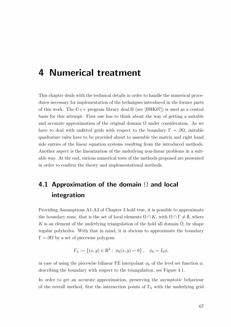
4 Numerical treatment
This chapter deals with the technical details in order to handle the numerical proce-
dures necessary for implementation of the techniques introduced in the former parts
of this work. The C++ program library deal.II (see [BHK07]) is used as a central
basis for this attempt. First one has to think about the way of getting a suitable
and accurate approximation of the original domain Ω under consideration. As we
have to deal with unfitted grids with respect to the boundary Γ = ∂Ω, suitable
quadrature rules have to be provided about to assemble the matrix and right hand
side entries of the linear equation systems resulting from the introduced methods.
Another aspect is the linearization of the underlying non-linear problems in a suit-
able way. At the end, various numerical tests of the methods proposed are presented
in order to confirm the theory and implementational methods.
4.1 Approximation of the domain Ω and local
integration
Providing Assumptions A1-A3 of Chapter 3 hold true, it is possible to approximate
the boundary zone, that is the set of local elements Ω ∩K, with Ω ∩ Γ 6= ∅, where
K is an element of the underlying triangulation of the hold all domain Ω, by shape
regular polyhedra. With that in mind, it is obvious to approximate the boundary
Γ = ∂Ω by a set of piecewise polygons
Γh :=
(x, y) ∈ R2 : φh(x, y) = 0, φh = Ihφ,
in case of using the piecewise bilinear FE interpolant φh of the level set function φ,
describing the boundary with respect to the triangulation, see Figure 4.1.
In order to get an accurate approximation, preserving the asymptotic behaviour
of the overall method, first the intersection points of Γh with the underlying grid
67

4 Numerical treatment
ΓhΓ
Figure 4.1: Example of a smooth domain Ω bordered by Γ and approximated piece-wise polygonal domain Ωh bordered by Γh on two local neighbouringelements in the boundary zone. The local domain Ωh is shaded grey.
have to be estimated. This is done element by element using the piecewise bilinear
approximation of the level set function φ, describing the boundary implicitly. A
suitable approximation of the original domain Ω then is given by the polygonal set
Ωh := (x, y) ∈ R2 : φh(x, y) < 0.
Each element K of the covering triangulation is marked whether it is part of Ω, being
part of the boundary zone (K ∩ Γ 6= ∅), or lying completely outside the domain of
interest, see Figure 4.2. According to that, there are three different cases to treat
with respect to numerical quadrature. The criterion is simply according to the signs
of the level set function, being evaluated at the vertices of an element. This can in
principle be generalized to the full three dimensional case, again by using for example
a nodewise interpolant of the original level set function, see [LN11]. However, the
local contributions to the stiffness matrix and right hand side are obtained regarding
the three possible cases.
Case 1:
The numerical integrations on the elements completely within Ω is handled the
standard way, using the deal.II routines for such tasks. The deal.II library provides
a whole zoo of quadrature rules. In particular we utilize Gaussian quadrature within
the implementations.
Case 2:
In the case of an element being part of the boundary zone, only the part lying within
the approximated domain, using the approximate polygonal boundary description
locally, is considered for integration regarding the weak formulation of the original
problem to be solved on Ω, see (3.2) and (3.28).
68

4.1 Approximation of the domain Ω and local integration
case 3
case 2
case 1
Figure 4.2: Example of a grid partitioned into those cells lying inside Ω (case 1,dark shaded), those in the boundary zone (case 2, white) and those cellsoutside Ω (case 3, bright shaded). Ω
∗h ⊂ Ω from (4.1) below is the union
of white and dark shaded elements.
A C++ class LocalIntegrationData, developed for handling this case, provides the
infrastructure for giving the elementwise information regarding local intersections
with the boundary, splitting the local geometry into elementary units, being quadri-
laterals, and giving the quadrature data (quadrature points and weights) in order to
generate a suitable quadrature rule needed for integration. Examples for this kind
of splitting are given in Figure 4.3.
In older implementations the splitting into elementary units has been into quadri-
laterals and triangles, the quadrature formulas being generated according to [Str71]:
Starting with a simple trapezoidal rule up to nine-point Gaussian quadrature rule
for a local rectangle.
The final implementation introduces a splitting into quadrilaterals only. This has
the advantage of bringing the whole lot of two dimensional quadrature rules pro-
vided by the deal.II library into play directly (deal.II by itself is only able to handle
quadrilateral and hexahedral geometries). The analogous things are provided by
the member functions of the LocalIntegrationData class in the case of contributions
from local boundary integrals on Γh.
69

4 Numerical treatment
Γh
1 2
3
Γh
1
Γh1
2
Figure 4.3: Examples for splitting the local approximations K ∩Ωh in the boundaryzone (marked in grey colour) into quadrilaterals for ease of elementwisecut-integration, required by the FD methods at hand. Left splittingresults in three, the right one into two quadrilaterals, while the one inthe middle can be treated directly.
Case 3:
The last situation, that is an element K lying completely outside the domain Ω,
can be handled in two ways. One is that integrations in order to fill the system
matrix are simply carried out for the bilinear form from regularization on that cell,
which is the standard way described in the former chapter. The other is handled
not exactly as in the original regularized method stated above. Instead of employing
the bilinear form b(·, ·) from (3.2), when dealing with an RDC system, or B(·, ·) for
an Oseen problem from Section 3.3, both ”living” on the whole grid, the forms
bh(uh, vh) := (∇uh,∇vh)Ω∗hor Bh(uh,vh) := (∇uh,∇vh)Ω∗h
are used for regularization along with the standard deal.II routines for integration.
The set Ω∗h is defined as
Ω∗h := K ∈ Th : K ⊂ Ω ∪ K ∈ Th : Γ ∩K 6= ∅, (4.1)
see Figure 4.2. The obvious alternative choice Ω = Ω∗h for the fictitious domain is
discussed and employed e.g. in [BH10a,BH10b].
Doing so, those degrees of freedom sharing no support with those lying in Ω∗h, are
constraint to zero. Note that this could be interpreted as an artificial jump of the
coefficients, but the convergence properties of the overall scheme is preserved, as on
the one hand we are only interested in the restriction of the solution to the domain
Ω and on the other hand the triangulation covers the interface describing the jump
exactly, see [Hac86]. However, we could have constrained the discrete solution of
70

4.2 A geometrical regularization method
problem (3.2)/(3.28) to another value in the case of not directly involved degrees of
freedom, as the discrete solution (as well as the underlying continuous one) has no
physical significance in this part of the fictitious domain.
4.2 A geometrical regularization method
In order to ensure the stability of the discrete problems resulting form the regularized
ones, and to get a suitable error analysis, Assumptions A1-A3 have been made in
Chapter 3. In practice Assumption A2 and A3 are not fulfilled on an arbitrary shape
regular mesh in general, at least not locally. Especially the violation of Assumption
A3 results in local instabilities in the numerical solution, to be observed as needle-
like peak singularities lying slightly outside the domain Ω. This is due to arbitrary
small entries in the system matrix, stemming from cut-integration on elements in
the boundary zone. One possibility to handle this problem would be to vary the
shape of an element: If necessary, slightly shift the vertices of an element in the
interface zone, taking into account the position of the intersection points, in order
to get a local inequality (3.6) fulfilled.
While this is a good choice in case of a stationary domain Ω, this could lead to
problems in the case of Ω = Ω(t). Another possibility of handling the drawback of
Assumption A3 is not fulfilled would be to slightly shift the intersection points of
the discrete zero level set and underlying grid instead of the vertices (if necessary),
in order to preserve the mesh, which is a central desire of our methods at hand.
Clearly, these shifts have to be made in such a way that the asymptotic behaviour
of the overall numerical method is preserved.
The strategy realized in the implementation, if an additional geometrical regulariza-
tion is desired, in case of an element K with K ∩ Γ 6= ∅, is the following. It clearly
orients itself on the definition of hΓD,K , see (3.3) and Figure 4.4 for an example:
• First compute the two intersection points of approximated boundary Γh and
∂K,
• estimate the distances d1, d2 of the in each case closest grid-nodes within Ω to
the intersections,
• given a number l ∈ (0, 1): If mind1, d2 < lhK , find this minimum and move
the affected intersection point(s), such that both points have a distance not
less then lhK to the closest inner node.
71
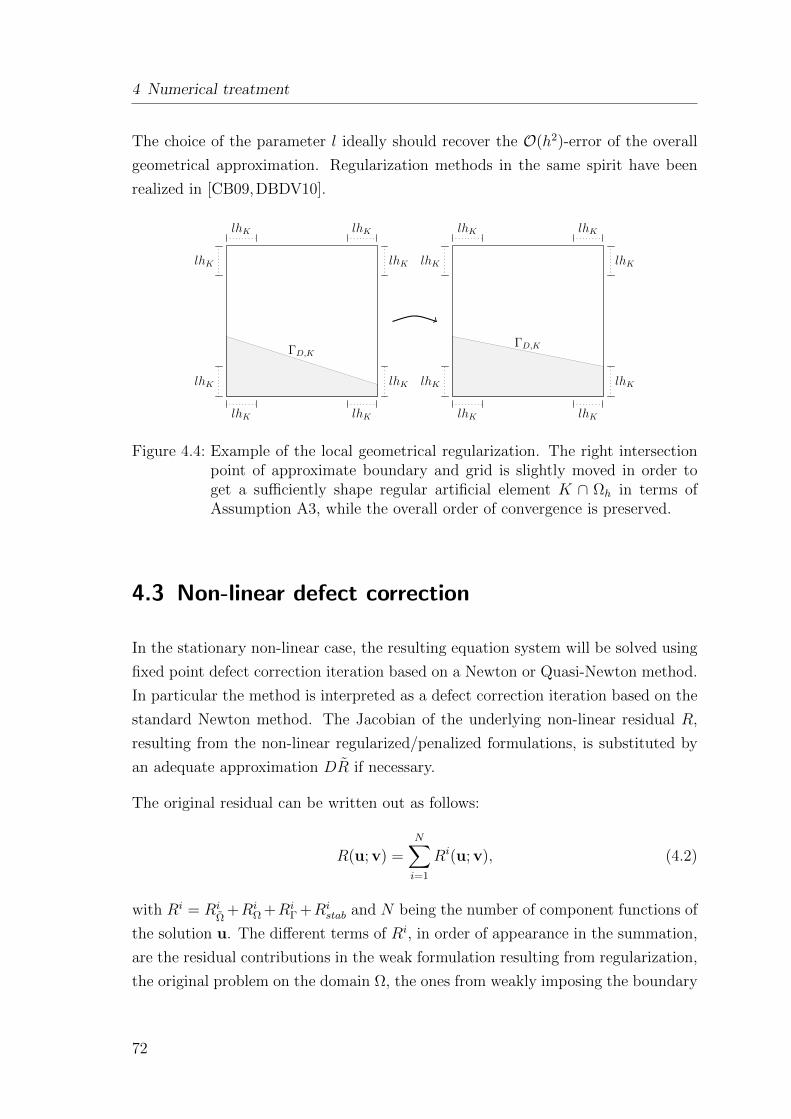
4 Numerical treatment
The choice of the parameter l ideally should recover the O(h2)-error of the overall
geometrical approximation. Regularization methods in the same spirit have been
realized in [CB09,DBDV10].
ΓD,K
lhK
lhK
lhK
lhK
lhK
lhK
lhK
lhK
ΓD,K
lhK lhK
lhKlhK
lhK
lhK lhK
lhK
Figure 4.4: Example of the local geometrical regularization. The right intersectionpoint of approximate boundary and grid is slightly moved in order toget a sufficiently shape regular artificial element K ∩ Ωh in terms ofAssumption A3, while the overall order of convergence is preserved.
4.3 Non-linear defect correction
In the stationary non-linear case, the resulting equation system will be solved using
fixed point defect correction iteration based on a Newton or Quasi-Newton method.
In particular the method is interpreted as a defect correction iteration based on the
standard Newton method. The Jacobian of the underlying non-linear residual R,
resulting from the non-linear regularized/penalized formulations, is substituted by
an adequate approximation DR if necessary.
The original residual can be written out as follows:
R(u; v) =N∑i=1
Ri(u; v), (4.2)
with Ri = RiΩ
+RiΩ +Ri
Γ +Ristab and N being the number of component functions of
the solution u. The different terms of Ri, in order of appearance in the summation,
are the residual contributions in the weak formulation resulting from regularization,
the original problem on the domain Ω, the ones from weakly imposing the boundary
72

4.3 Non-linear defect correction
condition and ensuring stability in case β 6= 0 and/or violation of the discrete inf-sup
condition by Galerkin least squares stabilization.
There are different kinds of pre-linearization in order to get efficient schemes for
different kinds of non-linear problems, taking the special behaviour of the underlying
problem into account. In all cases these methods have to lead to an approximate
Jacobian that is close enough to the original one in order to get an accurate scheme.
As such techniques are dependent on the special character of the problem, this will
be discussed in the application parts. Only a general procedure is described within
this section. Let i be an iteration index. The resulting fixed-point iteration then
writes:
1. Start with a predictor u0,
2. Find δui such that:
DR(ui; v)(δui) = −R(ui; v) ∀v ∈ V,
ui+1 := ui + αδui,
while ‖R(ui)‖ < tol.
In this procedure tol is a very small number, e.g. of order O(h2) at min while using
globally refined meshes, such that the error of the non-linear scheme is reduced
down to the approximation error, as bilinear FE are used for spatial discretization.
The parameter α is set to α := 2−k, with k being the smallest non-negative integer
such that ‖R(ui + 2−kδui)‖ < ‖R(ui)‖, in order to ensure the monotonicity of the
iteration scheme. In each iteration step the linear system for the next solution
update is solved via a CG solver in the symmetric, or a GMRES solver in the non-
symmetric case, in both cases preconditioned by a sparse LU or ILU decomposition
of the system matrix. The deal.II intern linear algebra module is utilized for that.
Moreover, the sparse direct solver UMFPACK, see [Dav04], can be used for solving
the resulting system or providing the LU decomposition.
73

4 Numerical treatment
4.4 Numerical accuracy
Several numerical examples with Ω = B1(0) are presented in order to demonstrate
the methods introduced during the former parts of this work with respect to the
model equations. We will concentrate on the case of pure Dirichlet problems, as
these essential boundary conditions are much harder to impose in a weak sense
then the natural Neumann conditions. Besides that and at first, we will test the
LocalQuadratureData class.
Ω
Ω1
Ω2
Ω3
Figure 4.5: The rectangular hold all domain Ω = (−1.2, 1.2)2 for test case0 with given circle, ellipse and rectangle embedded for testing thelocal integrator. The area meas
(Ω \ (Ω1 ∪ Ω2 ∪ Ω3)
)along with
meas(∂ (Ω1 ∪ Ω2 ∪ Ω3)
)have to be estimated by numerical integrations
using the LocalQuadratureData class member functions.
Test case 0
First, a non-trivial numerical test regarding the LocalQuadratureData class, used
for carrying out the cut-integrations in our FD method, is presented. The problem
at hand is: Estimate, by numerical integration, the area of Ω := Ω \ (Ω1 ∪ Ω2 ∪ Ω3),
with Ω being the rectangle (−1.2, 1.2)2 and
Ω1 := B0.25(−0.75,−0.75),
Ω2 :=
(x, y) ∈ R2 :
(x− 0.75
0.2
)2
+
(y − 0.75
0.25
)2
< 1
,
Ω3 :=
(x, y) ∈ R2 : |x|+ |y| < 0.3/√
2,
see picture 4.5. Moreover, the length of Γ := ∂ (Ω1 ∪ Ω2 ∪ Ω3) has to be estimated.
The tests are carried out starting with a four times up to ten times globally refined
74
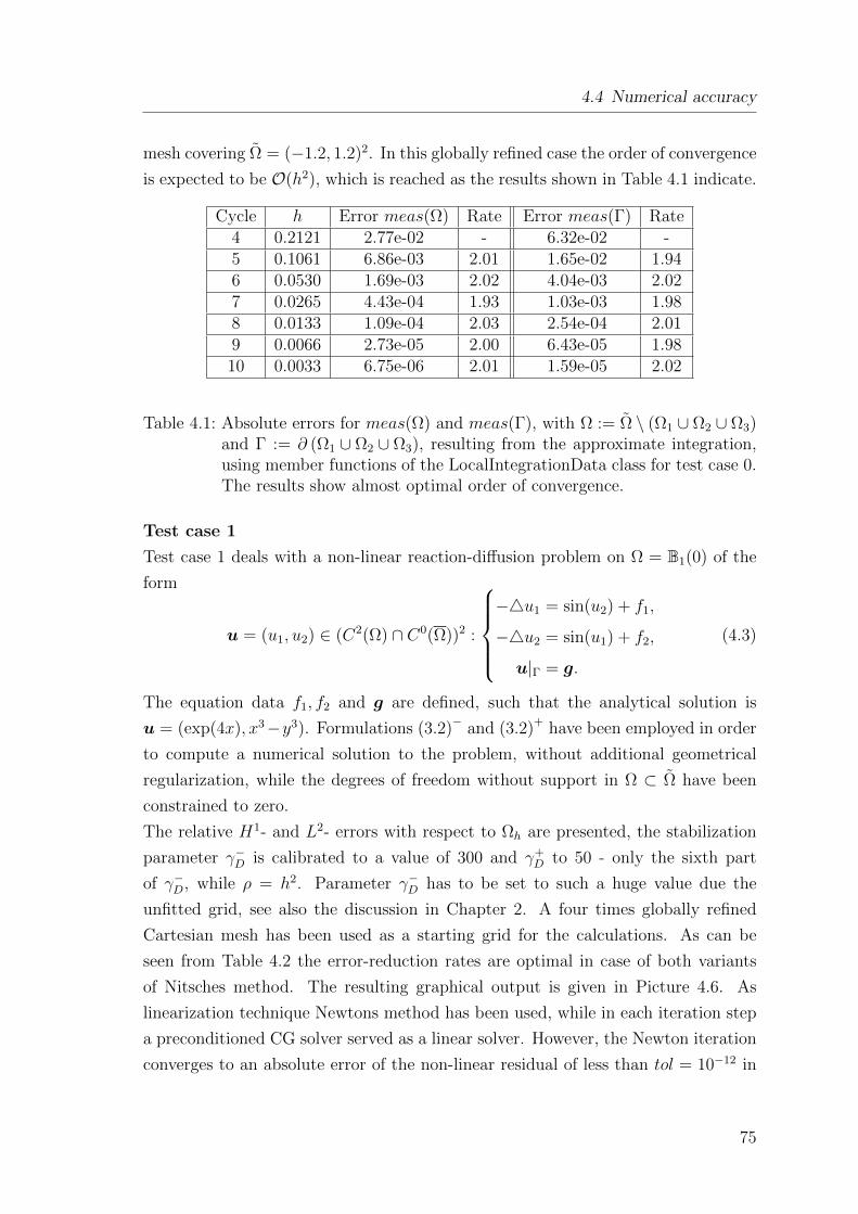
4.4 Numerical accuracy
mesh covering Ω = (−1.2, 1.2)2. In this globally refined case the order of convergence
is expected to be O(h2), which is reached as the results shown in Table 4.1 indicate.
Cycle h Error meas(Ω) Rate Error meas(Γ) Rate4 0.2121 2.77e-02 - 6.32e-02 -5 0.1061 6.86e-03 2.01 1.65e-02 1.946 0.0530 1.69e-03 2.02 4.04e-03 2.027 0.0265 4.43e-04 1.93 1.03e-03 1.988 0.0133 1.09e-04 2.03 2.54e-04 2.019 0.0066 2.73e-05 2.00 6.43e-05 1.9810 0.0033 6.75e-06 2.01 1.59e-05 2.02
Table 4.1: Absolute errors for meas(Ω) and meas(Γ), with Ω := Ω \ (Ω1 ∪ Ω2 ∪ Ω3)and Γ := ∂ (Ω1 ∪ Ω2 ∪ Ω3), resulting from the approximate integration,using member functions of the LocalIntegrationData class for test case 0.The results show almost optimal order of convergence.
Test case 1
Test case 1 deals with a non-linear reaction-diffusion problem on Ω = B1(0) of the
form
u = (u1, u2) ∈ (C2(Ω) ∩ C0(Ω))2 :
−4u1 = sin(u2) + f1,
−4u2 = sin(u1) + f2,
u|Γ = g.
(4.3)
The equation data f1, f2 and g are defined, such that the analytical solution is
u = (exp(4x), x3−y3). Formulations (3.2)− and (3.2)+ have been employed in order
to compute a numerical solution to the problem, without additional geometrical
regularization, while the degrees of freedom without support in Ω ⊂ Ω have been
constrained to zero.
The relative H1- and L2- errors with respect to Ωh are presented, the stabilization
parameter γ−D is calibrated to a value of 300 and γ+D to 50 - only the sixth part
of γ−D, while ρ = h2. Parameter γ−D has to be set to such a huge value due the
unfitted grid, see also the discussion in Chapter 2. A four times globally refined
Cartesian mesh has been used as a starting grid for the calculations. As can be
seen from Table 4.2 the error-reduction rates are optimal in case of both variants
of Nitsches method. The resulting graphical output is given in Picture 4.6. As
linearization technique Newtons method has been used, while in each iteration step
a preconditioned CG solver served as a linear solver. However, the Newton iteration
converges to an absolute error of the non-linear residual of less than tol = 10−12 in
75

4 Numerical treatment
h #Dofs ‖eρ1‖0,Ωh/‖u1‖0,Ωh Rate ‖eρ1‖1,Ωh/‖u1‖1,Ωh Ratesymmetric Nitsche method
0.2121 578 6.06e-02 - 1.57e-01 -0.1061 2178 1.53e-02 1.98 8.21e-02 0.930.0530 8450 3.54e-03 2.11 4.12e-02 1.000.0265 33282 8.51e-04 2.06 2.09e-02 0.980.0133 132098 2.07e-04 2.04 1.05e-02 0.990.0066 526338 5.11e-05 2.02 5.29e-03 0.99
asymmetric Nitsche method0.2121 578 6.03e-02 - 1.59e-01 -0.1061 2178 1.53e-02 1.98 8.31e-02 0.940.0530 8450 3.57e-03 2.10 4.12e-02 1.010.0265 33282 8.66e-04 2.04 2.12e-02 0.960.0133 132098 2.12e-04 2.03 1.06e-02 1.000.0066 526338 5.23e-05 2.02 5.35e-03 0.98
h #Dofs ‖eρ2‖0,Ωh/‖u2‖0,Ωh Rate ‖eρ2‖1,Ωh/‖u2‖2,Ωh Ratesymmetric Nitsche method
0.2121 578 5.35e-02 - 1.28e-01 -0.1061 2178 1.00e-02 2.42 6.03e-02 1.080.0530 8450 2.53e-03 1.99 2.98e-02 1.020.0265 33282 6.02e-04 2.07 1.49e-02 1.000.0133 132098 1.47e-04 2.04 7.47e-03 1.000.0066 526338 3.58e-05 2.03 3.73e-03 1.00
asymmetric Nitsche method0.2121 578 5.25e-02 - 1.29e-01 -0.1061 2178 9.89e-03 2.41 6.10e-02 1.080.0530 8450 2.52e-03 1.97 2.98e-02 1.030.0265 33282 6.06e-04 2.06 1.51e-02 0.980.0133 132098 1.48e-04 2.03 7.49e-03 1.010.0066 526338 3.63e-05 2.03 3.76e-03 0.99
Table 4.2: Relative H1(Ωh)- and L2(Ωh)-errors for test case 1, using both the sym-metric and asymmetric Nitsche formulations (3.2)∓. Above: For solutioncomponent 1, below: For solution component 2 - in all cases showingoptimal error-reduction rates.
76

4.4 Numerical accuracy
at most four steps, showing the quadratic reduction rate expected for the method.
As a pre-conditioner the LU decomposition of the Jacobian from the first iteration
has been used for all iteration steps.
Figure 4.6: Finite element solution of test case 1, with Ω := (−1.2, 1.2)2. Leftpicture-row: Components of the finite element solution after five globalrefinements. Right picture-row: Finite element solutions after eightglobal refinements.
77

4 Numerical treatment
Test case 2
Now a first example treating a convection dominated problem is considered using
the formulation (3.9)−:
−ε4u+ β · ∇u = f on B1(0),
u = 0 on S1,
where ε = 10−5, f = 1 and β = (1, 0). The right picture in Figure 4.7 shows the
solution resulting from the discrete regularized problem with additional SD enabled,
while the left one is obtained using the (regularized) standard Galerkin method. In
both cases it was γ−D = 300, ρ = h2, the SD stabilization parameters chosen due
to Chapter 3 with δ0 = 1. Both pictures show the discrete fictitious domain finite
element solution on a six times globally refined mesh, the fictitious domain being
(−1, 1)× (−1, 1). The right result is showing only small peaks next to the out-flow
boundary, which is due to the choice of Ω. The effect of the streamline diffusion
is clearly observable. The left one on the same grid shows the typical over- and
undershots applying in this situation, as no stabilization has been added.
Figure 4.7: Right: Finite element solution of the convection dominated problemfrom test case 2, stabilised by SD - only small oscillations are observable.Left picture: Finite element solution of the same problem based on thestandard Galerkin method, showing heavy over- and undershots.
78

4.4 Numerical accuracy
Test case 3
In order to show the accuracy of the stabilized method, now a linear scalar test-case
of a convection dominated RDC problem of the form
−ε4u+ β · ∇u+ u = f on B1(0),
u = gD on S1,
is presented, the stabilization parameters chosen as above. The data being defined
such that
u(x, y) =1
2
(1− tanh
( x
0.05
)),
which is a smoothed step-function and ε = 10−5. Again it is Ω = B1(0), while
Ω := (−1.2, 1.2)2, γ−D = 300 and ρ = h2, using formulation (3.9)−.
As in case of the first test, a four times globally refined Cartesian mesh has been used
as a starting grid. The results can be found in Figure 4.8 and Table 4.3, showing
optimal order of convergence with respect to both the H1(Ωh)- and L2(Ωh)-norms.
This is unless only O(h) can be granted a priori from (3.22), while in general O(h3/2)
can be expected from the common estimations found in the literature. A higher
order then expected is a circumstance often observed in case of the SD method,
see [Zho97].
h # Dofs ‖eρ‖0,Ωh/‖u‖0,Ωh Rate ‖eρ‖1,Ωh/‖u‖1,Ωh Rate0.1945 289 1.81e-01 - 7.65e-01 -0.0972 1089 3.55e-02 2.35 4.04e-01 0.920.0486 4225 8.76e-03 2.02 1.85e-01 1.120.0243 16641 2.04e-03 2.09 9.13e-02 1.020.0122 66049 4.79e-04 2.09 4.52e-02 1.010.0061 263169 1.15e-04 2.05 2.25e-02 1.000.0030 1050625 2.83e-05 2.03 1.12e-02 1.00
Table 4.3: Results for test case 3 using formulation (3.9)−, showing optimal order ofconvergence measured in relativeH1(Ωh)- as well as relative L2(Ωh)-norm.
79
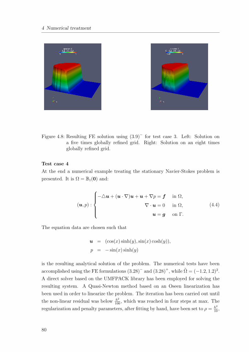
4 Numerical treatment
Figure 4.8: Resulting FE solution using (3.9)− for test case 3. Left: Solution ona five times globally refined grid. Right: Solution on an eight timesglobally refined grid.
Test case 4
At the end a numerical example treating the stationary Navier-Stokes problem is
presented. It is Ω = B1(0) and:
(u, p) :
−4u+ (u · ∇)u+ u+∇p = f in Ω,
∇ · u = 0 in Ω,
u = g on Γ.
(4.4)
The equation data are chosen such that
u = (cos(x) sinh(y), sin(x) cosh(y)),
p = − sin(x) sinh(y)
is the resulting analytical solution of the problem. The numerical tests have been
accomplished using the FE formulations (3.28)− and (3.28)+, while Ω = (−1.2, 1.2)2.
A direct solver based on the UMFPACK library has been employed for solving the
resulting system. A Quasi-Newton method based on an Oseen linearization has
been used in order to linearize the problem. The iteration has been carried out until
the non-linear residual was below h2
100, which was reached in four steps at max. The
regularization and penalty parameters, after fitting by hand, have been set to ρ = h2
10,
80

4.4 Numerical accuracy
while γ−D = 300 along with γ+D = 50, γ−1 = 10 and γ+
1 = 1. The elementwise constant
least squares stabilization parameters have been set to δK := h2K and γdiv = hK ,
which coincides with the choice in [RST08] for the case ν = 1.
Again starting point for the computations was a four times globally refined Cartesian
grid. The results regarding the usual error analysis in case of the symmetric and
asymmetric Nitsche method are shown in Table 4.4 and 4.5. A graphical output for
both velocity u and pressure p is shown in Figure 4.9 and 4.10.
It can be seen that both methods match each other regarding accuracy, while the
penalty parameter in case of the asymmetric Nitsche method can be chosen six times
smaller then in the symmetric Nitsche method. The reason again is the unfitted grid
along with the cut-integrations. The order of converge is almost optimal in case of
the velocity variable regarding both the L2- and H1-norm with respect to Ωh. The
order of convergence in the L2(Ωh)-norm for the pressure is suboptimal and about
1.7. As the a priori error bound in case of the linear symmetrical Stokes problem
(3.35) grants only an order 1, this still is a good result.
h # Dofs ‖eρu‖0,Ωh/‖u‖0,Ωh rate ‖eρu‖1,Ωh/‖u‖1,Ωh ratesymmetric Nitsche method
0.2121 578 5.67e-03 - 3.64e-02 -0.1061 2178 2.57e-03 1.16 1.51e-02 1.270.0530 8450 7.89e-04 1.70 7.12e-03 1.090.0265 33284 2.13e-04 1.89 3.46e-03 1.040.0133 132098 5.46e-05 1.96 1.69e-03 1.030.0066 526338 1.38e-05 1.99 8.44e-04 1.00
asymmetric Nitsche method0.2121 578 5.68e-03 - 3.53e-02 -0.1061 2178 2.57e-03 1.15 1.50e-02 1.240.0530 8450 7.89e-04 1.70 7.08e-03 1.080.0265 33284 2.12e-04 1.89 3.45e-03 1.040.0133 132098 5.46e-05 1.96 1.69e-03 1.030.0066 526338 1.38e-05 1.99 8.43e-04 1.00
Table 4.4: Relative error-reduction rates for the velocity component for test case4, measured in (L2(Ωh))
2- and (H1(Ωh))2-norm. The results are show-
ing almost optimal order of convergence in case of the symmetric andasymmetric Nitsche method, while using unfitted grids.
81

4 Numerical treatment
h # Dofs ‖eρp‖0,Ωh/‖p‖0,Ωh rate
symmetric Nitsche method0.2121 289 1.78e-01 -0.1061 1089 6.93e-02 1.360.0530 4225 2.12e-02 1.710.0265 16639 6.34e-03 1.740.0133 66049 1.94e-03 1.710.0066 263169 6.19e-04 1.65
asymmetric Nitsche method0.2121 289 1.76e-01 -0.1061 1089 6.87e-02 1.400.0530 4225 2.11e-02 1.700.0265 16639 6.31e-03 1.740.0133 66049 1.93e-03 1.710.0066 263169 6.16e-04 1.65
Table 4.5: Relative L2(Ωh)-error-reduction rates for the pressure component for testcase 4. The result shows an order of convergence of about 1.7 both forthe symmetric and asymmetric Nitsche method. This is being less thenoptimal, but still good and of higher order.
Figure 4.9: Numerical solution of the velocity variable for test case 4. Left: On afive times globally refined grid. Right: On an eight times globally refinedgrid. The degrees of freedom without support on Ω have been set to zero.
82
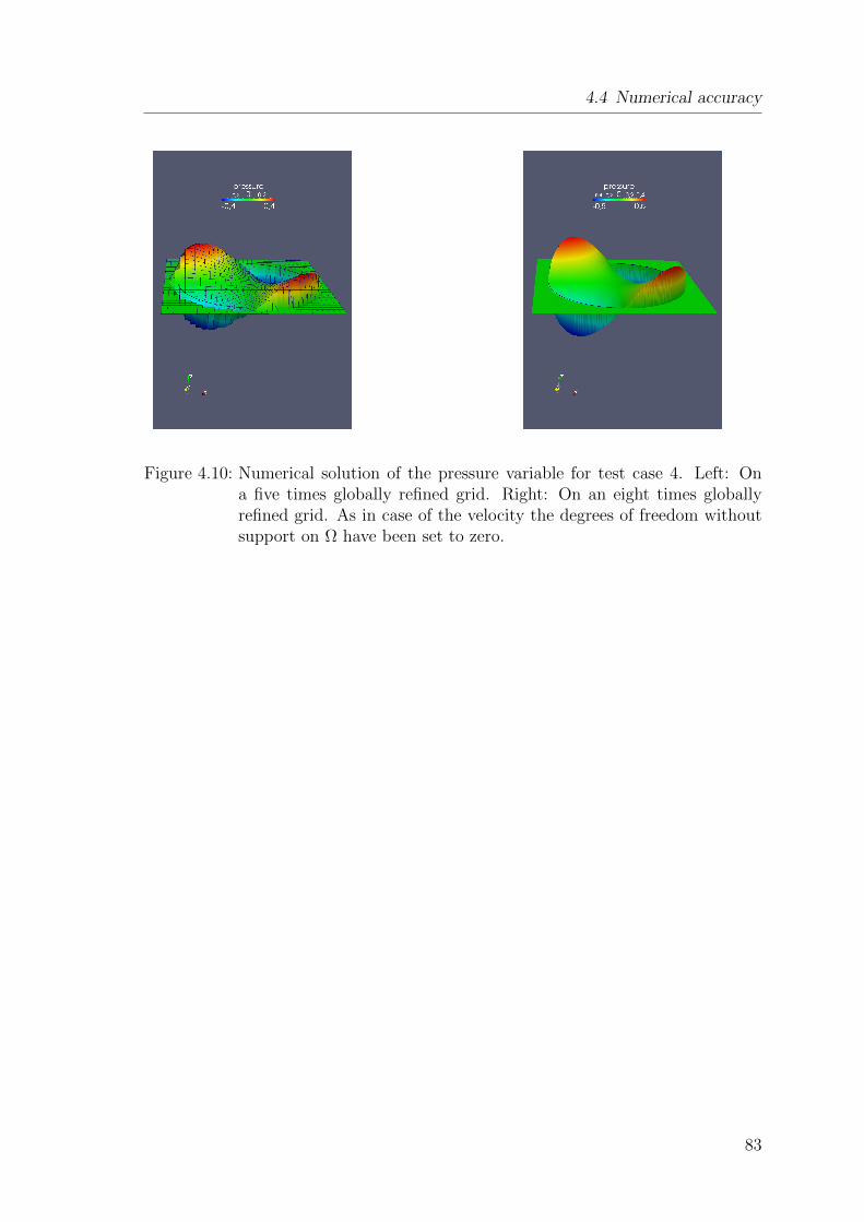
4.4 Numerical accuracy
Figure 4.10: Numerical solution of the pressure variable for test case 4. Left: Ona five times globally refined grid. Right: On an eight times globallyrefined grid. As in case of the velocity the degrees of freedom withoutsupport on Ω have been set to zero.
83

5 Applications
This chapter is addressed to various application in order to confirm, test and explore
the possibilities of the new FD methods. The focus within the application chapter is
solely on the asymmetric versions of Nitsches method, as stability is preferred over
high accuracy in our case, while the accuracy tests from Chapter 4 suggest that in
practice the difference in error-reduction is not very big. The outline is as follows:
First, a benchmark example regarding steady laminar flow around a plain cylinder is
presented, followed by a related unsteady flow problem using the same geometrical
setting. Moreover, we treat Boussinesq equations on a series of differently shaped
stationary domains. In the end a moving boundary value problem, again from the
flow section, is presented.
5.1 Application I: Steady laminar flow around a plain
cylinder
The flow around a plain cylinder at low Reynolds number is a widely used benchmark
problem in fluid dynamics. This is for good reason, as it belongs to a class of standard
problems in order to explore and test the flow around a rigid obstacle. The following
test problem was originally launched by Turek et al. in [ST96] as test case 2D-1.
Experimental data are available for comparison with plenty of existing numerical
data, while the underlying geometry is relatively simple but complicated enough to
provoke effects due to non-linearity as well as non-symmetry.
85

5 Applications
ΓC
Γin Γout
Γ0
Γ0(0, 0) (L, 0)
(0, H) (L,H)
Figure 5.1: Geometry of the first application: Plain rectangular canal Ω with inflowboundary Γin, outflow boundary Γout, non-slip boundary Γ0 and plaincylinder boundary ΓC . ΓC is described only implicitly by a characteristiczero level set.
5.1.1 Problem setting
The steady Navier-Stokes equations, in Ω := (0, L)× (0, H) \ BR(Pm), in the form:
−ν4u+ (u · ∇)u+∇p = 0 in Ω,
∇ · u = 0 in Ω,
u = 0 on Γ0 ∪ ΓC , (5.1)
u = g on Γin,
ν∂nu− np = 0 on Γout,
H = 0.41, L = 2.2, R = 0.05, Pm = (0.2, 0.2),
Um = 0.3, g = (4Umy(H − y)/H2, 0), ν = 10−3,
have to be solved. The benchmarking geometry is sketched in Figure 5.1.
86

5.1 Application I: Steady laminar flow around a plain cylinder
5.1.2 Numerical details
The benchmarking geometry sketched in Figure 5.1 more exact shows the fictitious
domain
Ω := (0, L)× (0, H)
for launching the FD method (3.28)+ based on regularization and the asymmet-
ric Nitsche method introduced in Section 3.3, but with the adjusted velocity and
pressure spaces
Vh :=
vh ∈
(C0(Ω)
)d: vh|K ∈ (Q1(K))d ∀K ∈ Th
∩(V 0
(Ω)),
Qh :=qh ∈ C0(Ω) : qh|K ∈ Q1(K) ∀K ∈ Th
,
with respect to a triangulation Th of the nearly Cartesian mesh. The inhomogeneous
inflow condition is enforced strongly in the first non-linear iteration step.
During the solution process, an Oseen linearization together with defect correction
takes place, substituting in the non-linear convection term the current solution by
the one from the last iteration step:
(ui+1h · ∇)ui+1
h −→ (uih · ∇)ui+1h .
For the numerical calculations we rely on the asymmetric Nitsche method (3.28)+
for its better stability properties. No further geometrical regularization (see Section
4.2) takes place during the computations.
While in the original problem the cylinder, or a geometrically approximation of the
latter, is cut out of the rectangular channel, the rigid obstacle is only represented
by a characteristic level set function describing the closed circle. However, under
normal circumstances, as the geometry is a relatively simple one, the usage of a
boundary-fitted grid, covering the inner boundary in an adequate way, is to be
preferred. But also it is a good test for a FD method.
The grids for numerical calculations stem from a standard rectangular triangulation
of the whole channel (see Figure 5.2 picture above), which then is three times (see
Figure 5.2 picture below), four and five times globally refined, while three local
refinement steps take place next to the inner cylinder boundary. More exact: An
87

5 Applications
element is refined, if itself or its neighbour is cut by the boundary of the cylinder at
some level during refinement. That is also what naturally happens in a boundary-
fitted method, as the grid is much more refined next to the cylinder in order to give
better a approximation of the curved cylinder boundary.
Figure 5.2: Above: Coarse pre-refined rectangular mesh for the fluid benchmarkproblem. Below: First computational mesh consisting of 4940 elements,originating from the one above by three times global followed by threetimes local refinement, in case an element or its neighbour is cut by thecylinder boundary at some level during refinement.
5.1.3 Benchmark quantities
Typical benchmark quantities are the following ones, being functionally dependent
on the pressure p and the velocity u:
J4p(p) := p(0.15, 0.2)− p(0.25, 0.2), (5.2)
Jdrag(u, p) :=2
U2D
∫ΓC
((2ν(∇u+∇uT )− pI
)· n)· ex ds, (5.3)
Jlift(u, p) :=2
U2D
∫ΓC
((2ν(∇u+∇uT )− pI
)· n)· ey ds, (5.4)
where U = 0.3, yielding a Reynolds number Re = UD/ν = 20. It is D = 2R and
ex, ey are the standard unit vectors in x- and y-direction. The drag coefficient Jdrag
defined by the boundary integral (5.3) physically gives a measure for the resistance
of the body within the fluid environment, while the lift coefficient Jlift from (5.4) is
related to the lift force regarding the flow around the cylinder.
88

5.1 Application I: Steady laminar flow around a plain cylinder
It is possible to represent the drag and lift coefficients by area integrals, which is
more robust and accurate compared to the boundary integral representation, see
e.g. [BR06].
In order to do so, and to treat things on the numerical level, we first migrate to the
discrete setting, i.e. ΓC is substituted by the piecewise polynomial approximation
ΓC,h, characterised by the nodewise Finite Element interpolant of a signed distance
function φcyl, describing ΓC by its zero level set, see Subsection 4.1.
Then, in the resulting weak formulation of (5.1) the test function is set to be
vd,h|Ω := (1 + φcyl,h, 0), vd,h|∂Ω := 0, (5.5)
vl,h|Ω := (0, 1 + φcyl,h), vl,h|∂Ω := 0. (5.6)
one after another.
Note that vd,h|ΓC,h = ex, vl,h|ΓC,h = ey and these test functions are contained in
(H10 (Ω))2. That along with backward partial integration, while utilizing consistency,
including the divergence-free constraint, gives alternatively:
Jdrag,h(u, p) := C[(
2νε(u), ε(vd,h))
Ωh+((u · ∇)u, vd,h
)Ωh−(p,∇ · vd,h
)Ωh
],
Jlift,h(u, p) := C[(
2νε(u), ε(vl,h))
Ωh+((u · ∇)u, vl,h
)Ωh−(p,∇ · vl,h
)Ωh
],
where C := 2
U2D
, ε(v) := 12
(∇v + ∇vT
)and Ωh is the polygonal implicitly given
approximation of Ω, see again Section 4.1.
From this the drag and lift coefficients are computed on the discrete level in all the
calculations.
5.1.4 Results and observations
The general behaviour of the fluid flow around the inner cylinder, along with the
resulting pressure and pressure isolines, both on the fictitious domain given above,
are shown in Figure 5.3. The pictures stem from numerical calculations on a mesh
with 137,133 degrees of freedom. As expected, the velocity magnitude is highest on
both sides of the inner boundary, while pressure maximum and minimum are to be
found on nearly diametrical points regarding the cylinder geometry in downstream
direction. A recirculation-zone is established downstream past the cylinder. Note
that due to the slightly non-symmetric geometry the solution is also slightly non-
89

5 Applications
symmetric, while the solutions are smooth and the flow is laminar, as the Reynolds
number is low.
Figure 5.3: General behaviour of the solution from the fluid benchmark problem onthe fictitious domain (0, 2.2)×(0, 0.41). Above: Velocity profile includingstreamlines; the resulting flow is laminar and slightly asymmetric due tothe implicitly given geometry. Below: Resulting pressure profile alongwith pressure contours. Note that the velocity field as well as the pressurevariable is defined on the whole mesh, as can be seen from the pictures.The cylinder is described by a characteristic level set function, with thezero level set contour shown in the pictures.
In order to minimize the number of parameters stemming from regularization, sta-
bilization and penalization, first a lower bound for the parameter γD has to be
identified. It turns out that setting γD = 30, along with γ1 = 1, gives sufficiently
good results, such that in all calculations within this section the Nitsche parameters
are pinned to these values.
Next the choice δK := δ0 minhK , h2K/ν, γdiv = δK is made, which is a possible
choice, with only one additional parameter δ0 originating from stabilization. Within
this configuration we first set ρ := h2K/10, a choice being ideal in case of the sym-
metric Stokes problem, see error estimate (3.35), and alternatively ρ := h3K . In order
to find a good value for the parameter δ0, several runs with δ0 ∈ 0.05, 0.1, 1 are
carried out.
As can be seen from Table 5.1, the results are in good agreement with the ones
published in the original paper [ST96] regarding accuracy and the number of degrees
of freedom to get a reliable result. Also the more recent results from [Win07] and
90

5.1 Application I: Steady laminar flow around a plain cylinder
[SGW11] are matched. In [Win07] different FE pairings and continuous interior
penalty stabilization have been used, while [SGW11] can be assigned to the fictitious
domain context, using XFEM and domain decomposition.
The values of drag, lift and pressure difference coefficients are all together within
the lower and upper bounds given in [ST96] after three refinement cycles, in case the
parameters of the method are chosen well. While the choices ρ = h2K/10 and ρ = h3
K
are sufficient along with δ0 = 0.1 or δ0 = 0.05, it can be seen from Table 5.1 that
δ0 = 1 gives no results within the claimed accuracy. Furthermore, the functional
values are quite sensitive especially regarding the choice of δ0, which is not a big
surprise.
91

5 Applications
γD = 30, γ1 = 1, γdiv = δK = δ0 minhK , h2K/ν
#Dofs hmin Jdrag Jlift J4pLower bound 5.5700 0.0104 0.1172Upper bound 5.5900 0.0110 0.1176
15693 0.00253 5.77830 0.01368 0.11375ρ = h2
K/10 43554 0.00126 5.66564 0.00913 0.11515δ0 = 1 137133 0.00063 5.62323 0.01012 0.11657
470925 0.00032 5.60420 0.00996 0.1172415693 0.00253 5.65120 0.00969 0.11761
ρ = h2K/10 43554 0.00126 5.60955 0.01244 0.11735
δ0 = 0.1 137133 0.00063 5.58971 0.01070 0.11738470925 0.00032 5.58307 0.01061 0.1174215693 0.00253 5.64743 0.00962 0.11803
ρ = h2K/10 43554 0.00126 5.60776 0.01265 0.11751
δ0 = 0.05 137133 0.00063 5.58848 0.01075 0.11746470925 0.00032 5.58145 0.01052 0.11744
15693 0.00253 5.69177 0.01186 0.11335ρ = h3
K 43554 0.00126 5.64366 0.00859 0.11499δ0 = 1 137133 0.00063 5.61725 0.01004 0.11652
470925 0.00032 5.60258 0.00993 0.1172315693 0.00253 5.57879 0.00742 0.11722
ρ = h3K 43554 0.00126 5.59040 0.01184 0.11719
δ0 = 0.1 137133 0.00063 5.58415 0.01064 0.11734470925 0.00032 5.58150 0.01058 0.1174215693 0.00253 5.57540 0.00733 0.117641
ρ = h3K 43554 0.00126 5.58869 0.01205 0.11735
δ0 = 0.05 137133 0.00063 5.58293 0.01067 0.11743470925 0.00032 5.58067 0.01063 0.11744
Table 5.1: Results for the benchmark quantities Jdrag, Jlift and J4p on four gridswith increasing subtly; bounds taken from [ST96]. The Nitsche param-eters have been fitted and pinned to γD = 30 and γ1 = 1, while ρ, γdivand δK are varied in order to find a reliable configuration of parame-ters. As can be seen, the choices γdiv = δK = δ0 minhK , h2
K/ν withδ0 ∈ 0.1, 0.05 give accurate results in case ρ ∈ h2
K/10, h3K. The num-
ber of degrees of freedom noteworthy to get results within the claimedaccuracy is 137,133 using the grids described above. The minimal celldiameter of a triangulation Th is hmin := mindiam(hK) : hK ∈ Th.
92
5.2 Application II: Non-steady flow around a plain cylinder
5.2 Application II: Non-steady flow around a plain
cylinder
Application II is addressed to non-steady flow around a plain cylinder. The general
ability of the developed methods for simulating problems from this field shall be
explored. In order to compare our results with reference solutions, known results to
be found on the FEATFLOW homepage by Turek (cf. [Tur98]) are used, utilizing
the same setting shown in Application I.
5.2.1 Problem setting
The non-steady Navier-Stokes equations, in Ω :=((0, L)× (0, H) \ BR(Pm)
)× I, in
the form:
∂tu− ν4u+ (u · ∇)u+∇p = 0 in Ω× I,
∇ · u = 0 in Ω× I,
u = 0 on(Γ0 ∪ ΓC
)× I, (5.7)
u = g on Γin × I,
ν∂nu− np = 0 on Γout × I,
have to be solved, with the same parameters L,H,R, Pm and ν already used in
Application I, but setting Um = 3/2. This finally yields a maximum Reynolds
number Re = 100, which means leaving the laminar regime. The inflow condition
is weighted by min1, t in order to provoke a distinct phase of oscillating flow. In
addition we set I := (0, 5], as well as ”starting from rest” initial conditions.
We will compare our results with the ones from [Tur98], where Turek shows how
hard it is to get reliable solutions in case of flow problems even in case of such a
relatively low Reynolds number. The drag and lift coefficients defined by (5.3) and
(5.4) have to be computed in each time step.
93

5 Applications
5.2.2 Numerical details
The common Oseen linearisation is used to treat the resulting non-linear system,
while utilizing the asymmetric Nitsche method (3.28)+. As we have to deal with a
time-dependent, non-linear problem, it is necessary to solve the resulting temporary
linear systems hundreds of times. During the solution process, assembling the matrix
and the LU-decomposition based pre-conditioner are the most time-consuming parts.
So in addition the system matrix is assembled completely new only as long as the
l2-norm of the non-linear residual is bigger than 10−5. This is a rather heuristic, but
economical strategy, in order to shorten the computational times along with getting
adequate solutions.
For time discretization the BDF2 scheme is used, with one implicit Euler step in
the beginning for construction of a second starting value. As a fully implicit scheme
is utilized, there are no too bad restrictions regarding the time step length. Never-
theless, the time step is chosen to be of about the same order of magnitude as the
smallest cell-diameter resulting from space discretization.
The coarse grid, on which the final one for the computations is based on, is shown in
Figure 5.4. The finer grids for the computations result from the coarse one by three
and four times global, followed by three time local refinement, similar to Application
I, while clearly the same definition for the discrete spaces is used in both cases. The
first grid then has 5964 cells and 18861 degrees of freedom, while the second has
18,036 cells and 56034 degrees of freedom. The smallest cell-diameter appearing is
hmin ≈ 0.00126, such that the time step is set to 4t = 0.001.
The parameters for regularization, stabilization and penalization are set to ρ =
0.1h2K , γdiv = δK = 0.1hK , γD = 50 and γ1 = 5, based on the observations of
Application I. By choosing 4t = O(hmin), this is a feasible choice in case of the
stabilization parameter.
Figure 5.4: Pre-refined near Cartesian grid, used for testing the new methods.
94
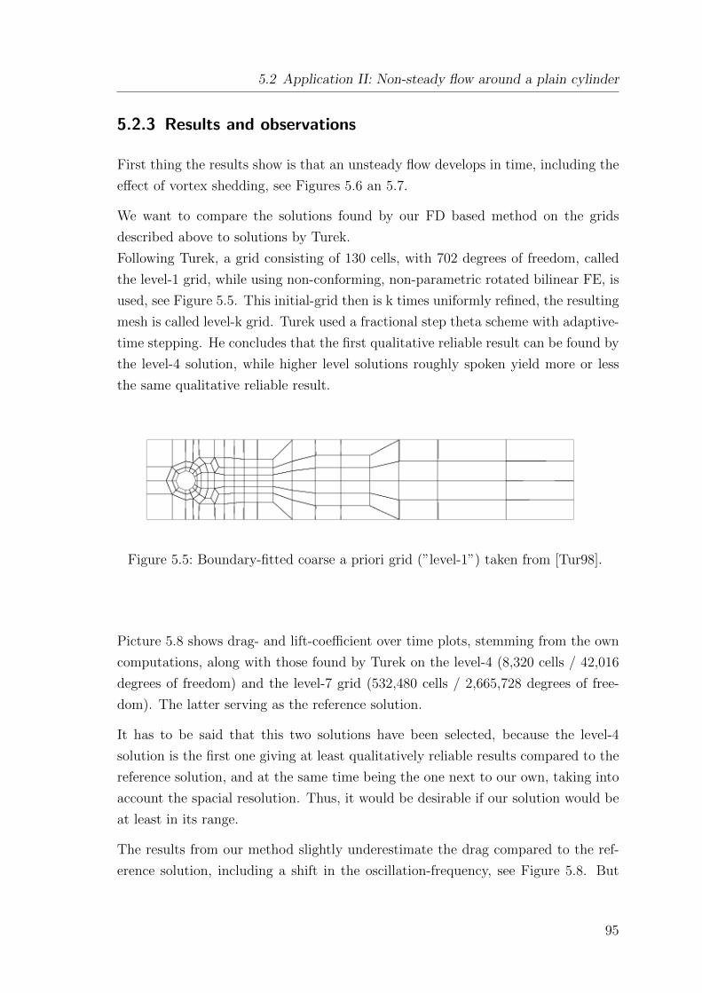
5.2 Application II: Non-steady flow around a plain cylinder
5.2.3 Results and observations
First thing the results show is that an unsteady flow develops in time, including the
effect of vortex shedding, see Figures 5.6 an 5.7.
We want to compare the solutions found by our FD based method on the grids
described above to solutions by Turek.
Following Turek, a grid consisting of 130 cells, with 702 degrees of freedom, called
the level-1 grid, while using non-conforming, non-parametric rotated bilinear FE, is
used, see Figure 5.5. This initial-grid then is k times uniformly refined, the resulting
mesh is called level-k grid. Turek used a fractional step theta scheme with adaptive-
time stepping. He concludes that the first qualitative reliable result can be found by
the level-4 solution, while higher level solutions roughly spoken yield more or less
the same qualitative reliable result.
Figure 5.5: Boundary-fitted coarse a priori grid (”level-1”) taken from [Tur98].
Picture 5.8 shows drag- and lift-coefficient over time plots, stemming from the own
computations, along with those found by Turek on the level-4 (8,320 cells / 42,016
degrees of freedom) and the level-7 grid (532,480 cells / 2,665,728 degrees of free-
dom). The latter serving as the reference solution.
It has to be said that this two solutions have been selected, because the level-4
solution is the first one giving at least qualitatively reliable results compared to the
reference solution, and at the same time being the one next to our own, taking into
account the spacial resolution. Thus, it would be desirable if our solution would be
at least in its range.
The results from our method slightly underestimate the drag compared to the ref-
erence solution, including a shift in the oscillation-frequency, see Figure 5.8. But
95

5 Applications
after the development of the unsteady state is reached, they are better then level-4
result by Turek, which for itself overestimates the drag in time. In case of the lift vs.
time result, our results are between the level-4 and the reference solution after the
oscillations are fully developed, but being closer to the reference solution. Moreover,
the solution on the finer grid gives better results, which is not a big surprise.
In view of using a method from the fictitious domain context, where often mean
values in case of drag and lift over time are taken for comparison after the fully de-
veloped oscillations phase is reached (see e.g. [YMUS99] and the literature therein),
this is a very good result. In particular, it has been shown that the new methods
are able to deal with unsteady flow problems in principle.
Figure 5.6: Velocity close-ups in the near wake of the inner cylinder. Left: Stream-lines and velocity magnitude short-time after the flow is fully developed,showing a (nearly) laminar behaviour at first. Right: Instantaneousstreamline and velocity-magnitude plot; vortex shedding appears.
96

5.2 Application II: Non-steady flow around a plain cylinder
Figure 5.7: Velocity magnitude (above) and pressure-contours (below) at final timeT = 5 in case of Application II.
2.8
2.9
3
3.1
3.2
3.3
1 1.5 2 2.5 3 3.5 4 4.5 5
dra
g
time (seconds)
Turek_4Turek_7
kru_5kru_6
-1
-0.5
0
0.5
1
1 1.5 2 2.5 3 3.5 4 4.5 5
lift
time (seconds)
Turek_4Turek_7
kru_5kru_6
Figure 5.8: Drag and lift coefficient time plots indicate that the FD based meth-ods give good results, without reaching the reference solution by Turek(Turek 7). The drag coefficient is slightly underestimated compared tothe reference solution, but in a better range compared to the level-4(Turek 4) solution by Turek. Here kru 5 indicates the result on thecoarser and kru 6 on the finer computational mesh, the latter being su-perior to the kru 5 result by itself. Analogous things are valid in case ofthe lift.
97

5 Applications
5.3 Application III: Boussinesq equations on
multi-connected domains.
Another application is the numerical treatment of the so called Boussinesq equa-
tions, meaning without much going into detail, that the Navier-Stokes equations are
coupled with an equation for temperature.
At first we give a short review on what this system of equations is describing phys-
ically, followed by the illustration of a test case on the unit rectangle, in order to
show the standard solution of the problem on a very simple domain for increasing
Rayleigh numbers.
The highlight then is the presentation of results from exploring the possibilities of
the proposed methods on the field of Boussinesq equations on geometrically compli-
cated domains, i.e. placing obstacles inside the unit-rectangle, while changing the
boundary conditions.
5.3.1 Description of the problem
As a basis for the model treated in this part of the work we assume Ω ⊂ R2,
with Γ := ∂Ω being partitioned into a Neumann- and a Dirichlet-part as usual. The
Boussinesq equations then can be written in the non-dimensional form (see [Ran08]):
∂tu−1
Re4u+ (u · ∇)u+∇p = − Ra
Re2PrgT in Ω× I, (5.8)
∇ · u = 0 in Ω× I, (5.9)
∂tT −1
RePr4T + u · ∇T = 0 in Ω× I, (5.10)
u = 0 on ∂Ω× I, (5.11)
T = TD on ΓD × I , ∂nT = TN on ΓN × I (5.12)
T = 0 , u = 0 in Ω× 0. (5.13)
In this system, the triple of unknowns (u, p, T ) consists of the usual pair (u, p) de-
scribing the flow pattern, which is driven only by the right hand side and thus by
(normalized) gravity g = (0,−1) and the remaining unknown, the scalar tempera-
ture field T , as can be seen from equations (5.8),(5.11) and (5.13).
98

5.3 Application III: Boussinesq equations on multi-connected domains.
The temperature T is described by the heat equation (5.10), where the velocity u
is part of the equation data driving the heat flow.
Besides the Reynolds number Re the relevant parameters appearing are:
- the Prandtl number Pr, being a material constant, more exact the ratio of
kinematic viscosity and thermal conductivity. We set Pr = 0.71, which is the
Prandtl number for atmospheric air,
- the Rayleigh number Ra, taking effectively the place of the Reynolds number,
as it is the relevant factor for stability of the system. It is known that in the
range Ra < 108 the resulting flow stays laminar, see [Has01]. Moreover, it can
be written Re =√RaPr
.
The Boussinesq equations in this form circumstantiate a slowly evolving temper-
ature field with constant density, while the temperature differences are relatively
small, such that the overall description of the in general far more complicated heat-
transfer process can be simplified, as several non-linear terms can be skipped for
being (nearly) constant or very small. Besides that we are treating a form of so
called natural convection, i.e. external sources influencing the system, besides the
ones already given, are neglected. For more information see e.g. [Ran08].
What happens from the physically point of view is, that due to thermal expansion
next to a heat source a buoyancy force appears, acting on the gas or fluid, transport-
ing material upward, while next to a heat sink the material is transported downward.
This interaction together with gravity causes a flow, in our case modelled by system
(5.8)-(5.13).
In order to demonstrate and explore the ability of the proposed methods to deal
with multi-connected domains, the Boussinesq equations and other akin ones, we
concentrate on the following basic setting, see Figure 5.9: The (in general fictitious)
domain Ω is the unit rectangle Ω := (0, 1)2, with its left and right hand sides
being heated or cooled, while no-heat-flux (perfect thermal insulation) conditions
are supposed on the upper and lower sides. Such configurations are very common in
the heat transfer community, and besides show a lot of interesting effects although
the underlying geometry is very simple.
99

5 Applications
gΩ
T = TH
u = 0
T = TC
u = 0
∂nT = 0, u = 0
∂nT = 0, u = 0
Figure 5.9: Original geometry and boundary conditions of the third application, itis Ω = (0, 1)2. The left boundary is heated, while the right one is cooled.Perfect insulation takes place at upper and lower boundary.
5.3.2 Numerical details
The whole system is treated in a fully implicit monolithic manner, meaning that a
non-linear defect-correction iteration, see Section 4.3, is applied in order to get an
approximate solution for the whole system describing (uh, ph, Th), while using the
techniques developed in this work.
The common Oseen linearisation, introduced in the last subsections, together with
substituting ui+1h · ∇T i+1
h by uih · ∇T i+1h in case of the heat equation, was used. In
all cases i being the iteration index of the non-linear scheme. The system matrix is
assembled completely new only as long as the non-linear residual is bigger than 10−3
in order to spare computation time, while getting adequate numerical solutions.
Time discretization happened by using the BDF2 scheme, with one implicit Euler
step in the beginning for construction of a second starting value.
After experimentations with four, five and six times globally refined grids, with
additional local refinement next to the Dirichlet boundaries, we choose a nearly
Cartesian grid with 4480 elements and 18956 degrees of freedom for discretization
in space as a basis for all computations, see left picture of Figure 5.10. As rather big
temperature gradients appear on the left and right side of the domain, the elements
on these sides are refined one time more then the rest, in order to avoid possible
numerical oscillations due to the boundary layers, as well as for better resolution of
the discontinuities in the boundary conditions. For the more complicated implicitly
given domains the meshes are based on the original one, but one time locally re-
100

5.3 Application III: Boussinesq equations on multi-connected domains.
finement took place next to the inner boundary components additionally, see Figure
5.10, right picture, for the case of Application III.2 as an example. In all cases it is
hmin =√
2/27 ≈ 0.011 and the time step is set to 4t = 2/100.
As criterion for reaching the steady-state we define:
‖(unh, pnh, T nh )− (un−1h , pn−1
h , T n−1h )‖∞
4t · ‖(unh, pnh, T nh )‖∞≤ 2 · 10−6,
where as always n is the time step number.
Figure 5.10: The heuristic refined rectangular meshes for the computations regard-ing Application III. Left: Grid for computations on the simple domainconsisting of 4480 elements, refinement took place next to the left andright sides in order to prevent oscillations due to mild boundary lay-ers. Right: Computational mesh for computations due to the multiple-connected domain of Application III.2, consisting of 5659 elements,originating from the left one by a single additional refinement next tothe inner boundaries. These boundary components are described onlyby a characteristic level set function.
The FE formulations (3.28)+ and (3.2)+ with the underlying adjusted discrete spaces
Vh :=
vh ∈
(C0(Ω)
)d: vh|K ∈ (Q1(K))d ∀K ∈ Th
∩(H1
0 (Ω))d,
Qh :=qh ∈ C0(Ω) : qh|K ∈ Q1(K) ∀K ∈ Th
∩ L2
0(Ω),
Wh :=Th ∈ C0(Ω) : Th|K ∈ Q1(K) ∀K ∈ Th
∩ V0(Ω),
101

5 Applications
with respect to the triangulation Th described above, are used for the numerical
solution process.
The complicated multi-connected domains Ω := Ω \ ω can be seen in the results-
section: A set of convex obstacles ω in each case is cut out of the fictitious domain
Ω, but only by describing these sets by characteristic level set functions.
In the standard case the regularization-terms in (3.2)+ and (3.28)+ are suppressed,
along with setting Γ := ∂Ω = ∅.
The author is aware of a potential mass-conservation problem due to the utilization
of stabilized FE, but this factor shall be not addressed here.
5.3.3 Results and observations
The grids described above are sufficient to resolve the instabilities within the given
range of laminar non-steady problems, while qualitative good solutions result from
the method. Streamline diffusion was disabled during the computations in case of
the temperature equation.
In case of the Navier-Stokes part the Galerkin least squares stabilization was used
nevertheless, as the discrete inf-sub condition still has to be circumvented, while
the divergence-free constraint has to be resolved most properly. By using a space
and time step of approximate the same order, an equal choice for the stabilization
parameters δK and γdiv, as in the steady case, has been made, along with the well
established choice δ0 = 0.1.
Now the results regarding several tasks are presented, first in text-form, followed by
graphical output of the steady-state solutions found by our solver. The Rayleigh
number is varied in case of the simple domain, while being fixed to Ra = 105 when
treating the complex domains.
102
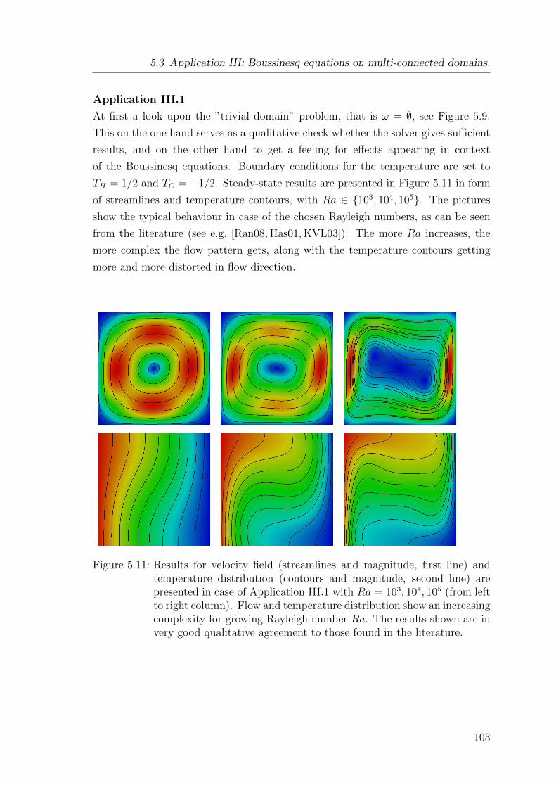
5.3 Application III: Boussinesq equations on multi-connected domains.
Application III.1
At first a look upon the ”trivial domain” problem, that is ω = ∅, see Figure 5.9.
This on the one hand serves as a qualitative check whether the solver gives sufficient
results, and on the other hand to get a feeling for effects appearing in context
of the Boussinesq equations. Boundary conditions for the temperature are set to
TH = 1/2 and TC = −1/2. Steady-state results are presented in Figure 5.11 in form
of streamlines and temperature contours, with Ra ∈ 103, 104, 105. The pictures
show the typical behaviour in case of the chosen Rayleigh numbers, as can be seen
from the literature (see e.g. [Ran08, Has01, KVL03]). The more Ra increases, the
more complex the flow pattern gets, along with the temperature contours getting
more and more distorted in flow direction.
Figure 5.11: Results for velocity field (streamlines and magnitude, first line) andtemperature distribution (contours and magnitude, second line) arepresented in case of Application III.1 with Ra = 103, 104, 105 (from leftto right column). Flow and temperature distribution show an increasingcomplexity for growing Rayleigh number Ra. The results shown are invery good qualitative agreement to those found in the literature.
103

5 Applications
Application III.2
This is the first task in order to deal with a complex multi-connected domain. The
updated configuration is sketched in Figure 5.12. The original boundary conditions
on ∂Ω are adopted from Application III.1, but a number of obstacles, described by
the techniques developed in this work, have been placed within the domain. On each
inner boundary component ∂nT = 0 and u = 0 are imposed weakly. The results are
shown is Figure 5.13.
Velocity field and temperature contours are presented, showing the expected be-
haviour. The velocity field shows a more complex, mainly clockwise, rotation com-
pared to the standard case in the first subapplication; including a shift of the recir-
culation zones. The obstacles are resolved well, while the weakly imposed non-slip
conditions for u can be observed. The temperature contours show the influence of
the perfect insulation at the implicitly given inner boundaries.
Application III.3
The next task deals with a non-slip/heated inner boundary, see Figure 5.14. The
original boundary conditions of Application III.1 on ∂Ω are adopted again. The
steady-state results can be observed in Figure 5.15.
What we see is a pretty symmetrical flow pattern as expected, along with two
recirculation zones next to the inner boundary, and near the area of maximal velocity
magnitude. The zero-boundary conditions u = 0 are matched very good. The
same is true for the inner Dirchlet conditions T = 1/10, which in interplay with
the strongly imposed conditions on ∂Ω drive the flow, for his part deforming the
temperature field.
Application III.4
At last we take a look on a situation where both left and right boundaries are cooled
to zero, with perfect insulation on the upper and lower sides. The main task is that
the only heat source now is at the implicitly given inner boundary. So the flow caused
by the inner boundary conditions has to drive the system mainly. The situation is
sketched in Figure 5.16, with three elliptical boundaries heated to +1/10.
The steady-state solution shows the expected slightly asymmetric flow behaviour
caused by the heated inner boundary, with recirculation zones resulting from the in-
terplay with the cooled outer boundary components, also reflected by the asymmet-
ric temperature contours. At the inner ellipses the Dirchlet conditions are matched
with high accuracy in case of both the temperature and the velocity.
104

5.3 Application III: Boussinesq equations on multi-connected domains.
T = 1/2
u = 0
T = −1/2
u = 0
∂nT = 0, u = 0
∂nT = 0, u = 0
Figure 5.12: Geometry and boundary conditions of Application III.2, it is still Ω =(0, 1)2. The left boundary is heated, while the right one is cooled.Perfect insulation takes place at upper and lower boundary, as well ason the inner boundary components. The latter are indicated by dashedlines.
Figure 5.13: Velocity field (left) and temperature (right) at steady-state are pre-sented in case of application III.2. The flow shows a more complexbehaviour than in the undisturbed case, with the obstacle placed inthe domain being flown around. The temperature contours show theinfluence of the perfect insulation at the inner boundaries, while theweakly imposed non-slip conditions for u can be observed.
105

5 Applications
u = 0T = 0.1
T = 0
u = 0
T = −1/2
u = 0
∂nT = 0, u = 0
∂nT = 0, u = 0
Figure 5.14: Geometry and boundary conditions of Application III.3. The left andright boundary components are cooled, while the inner boundary isheated. Perfect insulation takes place at upper and lower boundary.Non-slip conditions in case of velocity and a heated boundary for thetemperature are imposed weakly at the inner boundary component.
Figure 5.15: Steady-state velocity field (left) and temperature contours (right) arepresented in case of Application III.3. The flow shows a mainly clock-wise circulation as expected, with small recirculation zones next tothe right side of the heated cylinder. The temperature contours aredistorted in flow direction; the temperature 0.1-isoline matches nearlyperfect with the cylinder boundary, while the weakly imposed non-slipconditions for u can be observed.
106
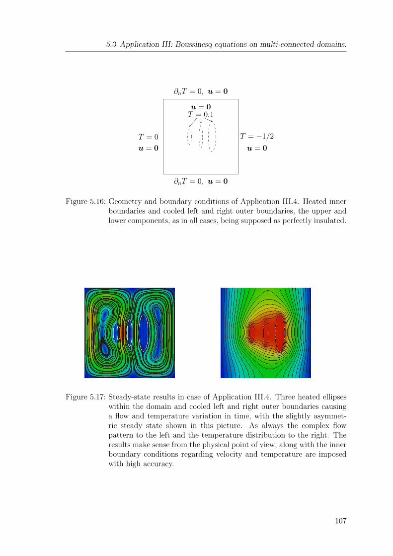
5.3 Application III: Boussinesq equations on multi-connected domains.
u = 0T = 0.1
T = 0
u = 0
T = −1/2
u = 0
∂nT = 0, u = 0
∂nT = 0, u = 0
Figure 5.16: Geometry and boundary conditions of Application III.4. Heated innerboundaries and cooled left and right outer boundaries, the upper andlower components, as in all cases, being supposed as perfectly insulated.
Figure 5.17: Steady-state results in case of Application III.4. Three heated ellipseswithin the domain and cooled left and right outer boundaries causinga flow and temperature variation in time, with the slightly asymmet-ric steady state shown in this picture. As always the complex flowpattern to the left and the temperature distribution to the right. Theresults make sense from the physical point of view, along with the innerboundary conditions regarding velocity and temperature are imposedwith high accuracy.
107

5 Applications
5.4 Application IV: Incompressible viscous flow
around a moving plain cylinder
As a non-steady application and experiment dealing with moving inner boundary,
and thus in essence with a time-dependent domain, we estimate numerically the
incompressible viscous flow around a moving plain cylinder in a box.
5.4.1 Problem setting
We follow Glowinski et al. [GPP96,GPP98], where the same configuration has been
used in order to test fictitious domain techniques based on boundary and volume
distributed Lagrange multipliers. The box is given by
Ω := (−0.35, 0.9)× (−0.5, 0.5),
the center (xc(t), yc(t)) of the disk
ω = ω(t) :=
(x, y) ∈ R2 : (x− xc)2 + (y − yc)2 ≤ R2; R = 0.125,
representing the cylinder, is moving between (0, 0) and (0.5, 0) with period four
along an a priori specified trajectory defined by
xc(t) := 0.25
(1− cos
(πt
2
)), yc(t) := −0.1 sin
(π
(1− cos
(πt
2
))). (5.14)
The geometry is sketched in Figure 5.18.
The mathematical formulation of the problem at hand on Ω = Ω(t) := Ω \ ω(t) can
be stated as:
∂tu− ν4u+ (u · ∇)u+∇p = 0 in Ω× I,
∇ · u = 0 in Ω× I,
u = 0 on Γ0 := ∂Ω× I, (5.15)
u = g on Γ := ∂ω × I,
u = 0 in Ω× 0.
108
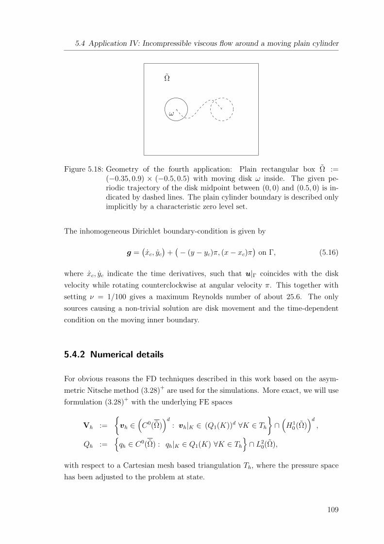
5.4 Application IV: Incompressible viscous flow around a moving plain cylinder
ω
Ω
Figure 5.18: Geometry of the fourth application: Plain rectangular box Ω :=(−0.35, 0.9) × (−0.5, 0.5) with moving disk ω inside. The given pe-riodic trajectory of the disk midpoint between (0, 0) and (0.5, 0) is in-dicated by dashed lines. The plain cylinder boundary is described onlyimplicitly by a characteristic zero level set.
The inhomogeneous Dirichlet boundary-condition is given by
g =(xc, yc
)+(− (y − yc)π, (x− xc)π
)on Γ, (5.16)
where xc, yc indicate the time derivatives, such that u|Γ coincides with the disk
velocity while rotating counterclockwise at angular velocity π. This together with
setting ν = 1/100 gives a maximum Reynolds number of about 25.6. The only
sources causing a non-trivial solution are disk movement and the time-dependent
condition on the moving inner boundary.
5.4.2 Numerical details
For obvious reasons the FD techniques described in this work based on the asym-
metric Nitsche method (3.28)+ are used for the simulations. More exact, we will use
formulation (3.28)+ with the underlying FE spaces
Vh :=
vh ∈
(C0(Ω)
)d: vh|K ∈ (Q1(K))d ∀K ∈ Th
∩(H1
0 (Ω))d,
Qh :=qh ∈ C0(Ω) : qh|K ∈ Q1(K) ∀K ∈ Th
∩ L2
0(Ω),
with respect to a Cartesian mesh based triangulation Th, where the pressure space
has been adjusted to the problem at state.
109

5 Applications
We prefer the asymmetric Nitsche method for its better stability purposes compared
to the symmetric version, as the inner boundary of the cylinder cuts the unfitted
grid in an uncontrolled manner, while moving in time. No additional geometrical
regularization has been used. This approach is closer to the first mentioned pa-
per [GPP96], where boundary distributed Lagrangian multipliers have been used in
order to enforce the boundary condition on Γ.
A more adequate description would be to enforce the rigid body motion on the whole
domain covered by the cylinder in each time step, which in fact is done for example
in [GPP98], using a second moving triangulation of the disk.
More on volume Lagrange multiplier based fictitious domain methods can be found
for example in [Glo03] and the literature therein. Alternatively, in Bonisch [Bon06]
a single mesh is used along with a projection technique, after solving suitable er-
satz problems with discontinuous coefficients on the whole domain, and adaptive
refinement in each time step.
5.4.3 Results and observations
Several computations took place on four and five times globally refined grids, using
adequate time steps. The implicit Euler and BDF2 2 schemes have been utilized for
semi-discretization in time. The common defect correction based Oseen linearisation
was used in order to solve the problem in each time step. For stabilization, after
some experiments, the parameters for stabilization and penalization have been set
to γdiv = δK = 0.1 minh, h2/ν, γD = 40, γ1 = 5 and ρ = 0.1h2. This is next to
the choice in Application I, and in case of the stabilization parameter feasible, as
the time step is chosen to be an O(h)-term.
The results are in very good qualitative agreement to the ones in [GPP96], using this
problem in order to get a feeling for such kinds of tasks, and to the ones in [GPP98],
where volume and boundary distributed Lagrangian multiplier based methods have
been compared on the same test configuration.
Thus, again following Glowinski [GPP96, GPP98], results in form of pressure con-
tours along with the streamlines for the discrete times 4.5, 5, 5.5, 6, 6.5, 7, 7.5, 8 are
shown within the next figures, resulting from computations using the implicit Euler
scheme with a time step 4t = 1/64 ≈ 0.0156 on the five times uniformly refined
grid, with h ≈ 0.041. In case of the higher order time stepping scheme, the time
parameter was doubled, while the results look similar to the ones from the Euler
scheme.
110

5.4 Application IV: Incompressible viscous flow around a moving plain cylinder
Figure 5.19: Resulting pressure contours (left column) and streamlines (right col-umn) at times t = 4.5, 5, 5.5, 6 (from top to bottom) in case of Applica-tion IV. The disk is moving from left to right. The colour scale is fromblue (low pressure/velocity magnitude) to red (high pressure/velocitymagnitude).
111

5 Applications
Figure 5.20: Resulting pressure contours (left column) and streamlines (right col-umn) at times t = 6.5, 7, 7.5, 8 (from top to bottom) in case of Applica-tion IV. The disk is moving from right to left. The colour scale is fromblue (low pressure/velocity magnitude) to red (high pressure/velocitymagnitude).
112

6 Discussion and Outlook
New methods belonging to the fictitious domain context based on the results and
ideas of Glowinski et al. have been introduced and analyzed, both from the continu-
ous and the discrete numerical level. In two dimensions, symmetric and asymmetric
variants of Nitsches method have been used in order to impose essential boundary
conditions in case of the discrete methods.
The level set method was utilized in order to describe the underlying geometry the
equations are defined on. The new methods are able to handle very general non-
linear, time-dependent and asymmetric problems of second order, including saddle
point problems in form of Stokes and Navier-Stokes equations.
Numerical analysis took place regarding different special cases, separated with re-
spect to the typical aspects causing trouble, as to mention dominant convection
and circumventing a discrete inf-sub condition in case of the Stokes and Navier-
Stokes equations. Streamline diffusion/Galerkin least squares stabilization was used
to resolve such kind of problems.
From the practical point of view, the asymmetric versions of Nitsches method turn
out to be preferable in view of their better stability properties, when used in the FD
context, while numerical tests suggest, that not too much loss regarding the error
reduction rates happens compared to the symmetrical versions.
The methods have been utilized successfully in view of several applications, after
the task of numerical accuracy was addressed. In the field of laminar and unsteady
plain flow problems, slow thermal convection on multi-connected domains, as well
as in rigid body motion, the methods seem to have a lot of potential; at least in two
dimensions, while it of course would be possible to generalize the method to three
dimensions as well.
Among the advantages of the developed methods are the usage of standard FE
spaces, along with the usage of Cartesian and near Cartesian grids, and high flexi-
bility regarding the underlying geometry.
113
6 Discussion and Outlook
Drawbacks should be mentioned also: A lot of parameters for stabilization, regu-
larization and so on have to be fitted. Besides that, the condition of the resulting
discrete problems requires special care by a good pre-conditioner, in case of using
an iterative solver.
Obvious possibilities for extensions and interesting future tasks would be in the
field of three dimensional problems. In view of the last point, but also independent,
exploration in the area of better local refinement strategies would be desirable.
Especially strategies based on dual weighted residual techniques, in order to produce
economical grids, could be a great enrichment.
Moreover, economical pre-condition techniques, for example from the multi-grid
section, would be of interest.
Another obvious task to be mentioned is the exploration of fluid-structure interaction
problems, like numerical simulation of glacier motion or droplet evaporation, using
the methods at hand. In addition to that, fictitious domain approaches similar to
the ones used in this work could potentially be applied to other common fields of
continuum mechanics besides the Navier-Stokes equations.
114

Bibliography
[ABCM02] Douglas N Arnold, Franco Brezzi, Bernardo Cockburn, and L Donatella
Marini. Unified analysis of discontinuous galerkin methods for elliptic
problems. SIAM Journal on Numerical Analysis, 39(5):1749, 2002.
[AH09] K. Atkinson and Weimin H. Theoretical Numerical Analysis. Springer,
3. edition, 2009.
[Bab73a] I. Babuska. The Finite Element Method with Lagrangian Multipliers.
Numer Math., 20:179–192, 1973.
[Bab73b] I. Babuska. The Finite Element Method with Penalty. Mathematics of
Computation, 27(122), April 1973.
[BBH10] R. Becker, E. Burman, and P. Hansbo. A hierarchical NXFEM for
fictitious domain simulations. CHALMERS PREPRINT 2010:24, , 2010.
[BE86] J. W. Barrett and C. M. Elliott. Finite Element Approximation of the
Dirichlet Problem Using the Boundary Penalty Method. Numer. Math,
49:343–366, 1986.
[Bec02] R. Becker. Mesh adaption for Dirichlet flow control via Nitsche’s
method. Commun. Numer. Meth. Engng, 18:669–680, 2002. (DOI:
10.1002/cnm.529).
[BF91] F. Brezzi and M. Fortin. Mixed and hybride finite element methods.
Springer, 1991.
[BF09] Erik Burman and Miguel A. Fernandez. Stabilization of explicit coupling
in fluid–structure interaction involving fluid incompressibility. Computer
Methods in Applied Mechanics and Engineering, 198(5–8):766 – 784,
2009.
[BH91] H. J. C. Barbosa and T. J. R. Hughes. The finite element method with
Lagrangian multipliers on the boundary: circumventing the Babuska-
115
Bibliography
Brezzi condition. Computer Methods in Mechanics and Engineering,
85(1):109–128, 1991.
[BH10a] E. Burman and P. Hansbo. Fictitious domain finite element methods
using cut elements: I. A stabilized Lagrange multipier method. Comput.
Methods Appl. Mech. Eng., 2010. (2010), doi:10.1016/j.cma.2010.05.011.
[BH10b] E. Burman and P. Hansbo. Fictitious domain finite element meth-
ods using cut elements: II. A stabilized Nitsche method. CHALMERS
PREPRINT 2010:25, 2010.
[BHK] W. Bangerth, T. Heister, and G. Kanschat. deal.II Differential Equa-
tions Analysis Library,Technical Reference. http://www.dealii.org.
[BHK07] W. Bangerth, R. Hartmann, and G. Kanschat. deal.II – a general pur-
pose object oriented finite element library. ACM Trans. Math. Softw.,
33(4):24/1–24/27, 2007.
[BHS01] Roland Becker, Peter Hansbo, and Rolf Stenberg. A finite element
method for domain decomposition with non-matching grids. Technical
report, MATH. MODEL. ANAL. NUMER, 2001.
[BM97] I. Babuska and J. Melenk. The Partition of Unity Method. International
Journal for Numerical Methods in Engineering, 40:727–758, 1997.
[Bon06] S. Bonisch. Adaptive Finite Element Methods for Rigid Particulate Flow
Problems. PhD thesis, Universitat Heidelberg, 2006.
[BR06] M. Braack and T. Richter. Solutions of 3D Navier-Stokes bench-
mark problems with adaptive finite elements. Computers and Fluids,
35(4):372–392, 2006.
[Bra98] M. Braack. An Adaptive Finite Element Method for Reactive-Flow Prob-
lems. PhD thesis, University of Heidelberg, 1998.
[Bra03] D. Braess. Finite Elemente. Springer, 3. edition, 2003.
[CB03] J. Chessa and T. Belytschko. An enriched finite element method and
level sets for axisymmetric two-phase flow with surface tension. Internat.
J. Numer. Methods Engrg., 43:50–67, 2003.
[CB09] R. Codina and J. Baiges. Approximate imposition of boundary condi-
tions in immersed boundary methods. International Journal for Numer-
ical Methods in Engineering, 2009.
116
Bibliography
[Dav04] Timothy A. Davis. Algorithm 832: Umfpack v4.3—an unsymmetric-
pattern multifrontal method. ACM Trans. Math. Softw., 30(2):196–199,
June 2004.
[DBDV10] G. Dupire, J. P. Boufflet, M. Dambrine, and P. Villon. On the necessity
of Nitsche term. Applied Numerical Mathematics, 60:888–902, 2010.
[Duc10] M. Ducker. Numerical analysis of Cauchy-type problem arising in elec-
trical engineering. PhD thesis, University of Siegen, 2010.
[EB05] C. Engwer and P. Bastian. A Discontinuous Galerkin method for simu-
lations in complex domains. IWR-Preprint, 2005.
[EGK08] C. Eck, H. Garcke, and P. Knabner. Mathematische Modellierung.
Springer, 2008.
[GG95] V. Girault and R. Glowinski. Error Analysis of a Fictitious Domain
Method Applied to a Dirichlet Problem. Japan J. Indust. Appl. Math.,
(12):487–514, 1995.
[Glo03] R. Glowinski. Numerical Methods for Fluids (Part 3). North-Holland,
2003.
[GP92] R. Glowinski and W. T. Pan. Error estimates for fictitious do-
main/penalty/finite element methods. Calcolo, 29(125), 1992.
[GPH+99] Roland Glowinski, Tsorng-Whay Pan, Todd I. Hesla, Daniel D. Joseph,
and Jacques Periaux. A distributed lagrange multiplier/fictitious do-
main method for flows around moving rigid bodies: Application to par-
ticulate flow. International Journal for Numerical Methods in Fluids,
30(8):1043–1066, 1999.
[GPP96] R. Glowinski, T. W. Pan, and J. Periaux. Fictitious Domain Methods for
Incompressible Viscous Flow around Moving Rigid Bodies. Proceedings
of MAFELAP 1996, 1996.
[GPP98] R. Glowinski, T. W. Pan, and J. Periaux. Distributed Lagrange multi-
plier methods for incompressible viscous flow around moving rigid bod-
ies. Comput. Methods Appl. Mech. Engrg., 151, 1998.
[GPWZ96] R. Glowinski, W. T. Pan, R. O. Wells, and X. Zhou. Wavelet and Finite
Element Solutions for the Neumann Problem Using Fictitious Domains.
JOURNAL OF COMPUTATIONAL PHYSICS, (126):40–51, 1996.
117

Bibliography
[GR94] C. Grossmann and H.-G. Roos. Numerik partieller Differentialgleichun-
gen. Teubner Studienbucher, 2. edition, 1994.
[GR07] S. Gross and A. Reusken. An extended pressure finite element space for
two-phase incompressible flows with surface tension. Journal of Com-
putational Physics, (224):40–58, 2007.
[GT83] D. Gilbarg and N. S. Trudinger. Elliptic Partial Differential Equations
of Second Order. Springer, 1983.
[Hac86] W. Hackbusch. Theorie und Numerik elliptischer Differentialgleichun-
gen. Teubner, 1986.
[Han05] P. Hansbo. Nitsches method for interface problems in computational
mechanics. GAMM-Mitt, 2005. 28/2 (2005) 183-206.
[Has01] H. Haschke. Splitting-Techniken zur spektralen Approximation der
Navier-Stokes- und Boussinesq-Gleichungen. PhD thesis, Universitat
Essen, 2001.
[Hei08] C.-J. Heine. Finite element methods on unfitted meshes. ISSN 1439-
962-X, Preprint Nr. 9/2008-28.10.2008, 2008. Universitat Freiburg.
[HH03] Peter Hansbo and Joakim Hermansson. Nitsche’s method for coupling
non-matching meshes in fluid-structure vibration problems. Computa-
tional Mechanics, 32(1-2):134–139, 2003.
[HN81] C. W. Hirt and B. D. Nichols. Volume of fluid (vof) method for the
dynamics of free boundaries. J. Comp. Phys., 39:301–225, 1981.
[HS97] W. Hackbusch and S. A. Sauter. Composite Finite Elements for the
approximation of PDEs on domains with complicated micro-structures.
Numer. Math., 75(4), 1997.
[HY09] J. Haslinger and Renard Y. A new fictitious domain approach inspired
by the extended finite element method. SIAM Journal on Numerical
Analysis, 47(2):1474–1499, 2009.
[Jim04] P. K. Jimack. Adaptive Algorithms for Free-Surface Flow Problems.
2004. http://www.scs.leeds.ac.uk/pkj/Papers/Conf-I/J04a.pdf.
[Joh90] C. Johnson. Numerical solution of partial differential equations by the
finite element method. Cambridge University Press, 3. edition, 1990.
118

Bibliography
[JS08] M. Juntunen and R. Stenberg. Nitsches method for general bound-
ary conditions. Mathematics of Computation, (S 0025-5718(08)02183-2),
2008.
[KVL03] Khalil Khanafer, Kambiz Vafai, and Marilyn Lightstone. Buoyancy-
driven heat transfer enhancement in a two-dimensional enclosure uti-
lizing nanofluids. International Journal of Heat and Mass Transfer,
46(19):3639 – 3653, 2003.
[LB08] A. J. Lew and G. C. Buscaglia. A discontinuous-Galerkin-based im-
mersed boundary method. Int. J. Numer. Meth. Engng., 76(4), 2008.
[LGT81] J. L. Lions, R. Glowinski, and R. Tremolieres. Numerical Analysis of
Variational Inequalities. North Holland, 1981.
[LN11] A. Lew and M. Negri. Optimal convergence of a discontinuous-alerkin-
based immersed boundary method. ESAIM:Mathematical Modelling and
Numerical Analysis, (45):651–674, 2011.
[LP00] M. Lai and C. S. Peskin. An immersed boundary method with for-
mal second-order accuracy and reduced numerical viscosity. Journal of
Computational Physics, 160:705–719, 2000.
[MDB99] N Moes, J. Dolbow, and T. Belytschko. The Partition of Unity Method.
International Journal for Numerical Methods in Engineering, 46(1):131–
150, 1999.
[Nit71] J. Nitsche. Uber ein Variationsprinzip zur Losung von Dirichlet-
Problemen bei der Verwendung von Teilramen, die keinen Randbedin-
gungen unterworfen sind. Abhandlungen aus dem mathematischen Sem-
inar der Universitat Hamburg, 36:9–15, Springer, 1971.
[OS88] S. Osher and J.A. Sethian. Front propagating with curvature-dependent
speed: algorithms based on hamilton-jacobi formulations. J. Comput.
Phys., 79:1–49, 1988.
[Pes72] C. S. Peskin. Flow patterns around heart valves: A digital computer
method for solving the equations of motion. PhD thesis, Albert Einstein
College of Medicine, 1972.
[Pes02] C. S. Peskin. The immersed boundary method. Acta Numerica, pages
479–517, 2002. DOI: 10.1017/S0962492902000077.
119

Bibliography
[PS08] Daniel Peterseim and Stefan A. Sauter. The composite mini element -
coarse mesh computation of stokes flows on complicated domains. SIAM
J. Numer. Anal., 46:3181–3206, September 2008.
[PS09] D. Peterseim and S. Sauter. Finite Element Methods for the Stokes
Problem on Complicated Domains. , 2009.
[QV94] A. Quarteroni and A. Valli. Numerical approximation of partial differ-
ential equations. Springer Verlag, Berlin, 1994.
[QV05] A. Quarteroni and A. Valli. Domain Decomposition Methods for Partial
Differential Equations. Clarendon Press, Oxford, 2005.
[Ran06] R. Rannacher. Numerische Mathematik 2. Vorlesungsskriptum SS 2006,
2006.
[Ran08] R. Rannacher. Numerische Mathematik 3. Vorlesungsskriptum
WS2004/2005, 2008.
[Rec06] M. Rech. An adaptive two-scale approach to the non-conforming ap-
proximation of Dirichlet problems on complicated domains. PhD thesis,
Universitat Zurich, 2006.
[RST08] H.-G. Roos, M. Stynes, and L. Tobiska. Robust Numerical Methods for
Singularly Perturbed Differential Equations. Springer, 2. edition, 2008.
[SCMB01] N. Sukumar, D. L. Chopp, N. Moes, and T. Belytschko. Modeling holes
and inclusions by level sets in the extended finite-element method. Com-
puter Methods in Applied Mechanics and Engineering, 190(46-47):6183–
6200, 2001.
[Set99] J.A. Sethian. Level Set Methods and Fast Marching Methods. Cambridge
University Press: Cambridge, UK, 2. edition, 1999.
[SFSO97] Mark Sussman, Emad Fatemi, Peter Smereka, and Stanley Osher. An
improved level set method for incompressible two-phase flows. Comput-
ers and Fluids, 27:663–680, 1997.
[SGW11] Shadan Shahmiri, Axel Gerstenberger, and Wolfgang A. Wall. An xfem-
based embedding mesh technique for incompressible viscous flows. In-
ternational Journal for Numerical Methods in Fluids, 65(1-3):166–190,
2011.
120

Bibliography
[ST96] M. Schafer and S. Turek. Benchmark computations of laminar flow
around a cylinder. Technical report, Universitat Heidelberg, Preprint
SFB 359, 1996.
[Ste95] R. Stenberg. On some techniques for approximating boundary conditions
in the finite element method. Journal of Computational and Applied
Mathematics, (63):139–148, 1995.
[Ste98] R. Stenberg. MORTARING BY A METHOD OF J.A. NITSCHE. Com-
putational Mechanics, 1998.
[Str71] A.H. Stroud. Approximate calculation of multiple integrals. Prentice-
Hall, 10. edition, 1971.
[SZ90] Ridgway L. Scott and Shangyou Zhang. Finite Element Interpolation of
Nonsmooth Functions Satisfying Boundary Conditions. Mathematics of
Computation, 54(190):483–493, 1990.
[Tur98] S. Turek. The ‘DFG-Benchmark 1995/6’: Channel flow around a circle
at Re=100, 1998. http://www.mathematik.uni-dortmund.de/ featflow.
[Win07] C. Winkelmann. INTERIOR PENALTY FINITE ELEMENT AP-
PROXIMATION OF NAVIER-STOKES EQUATIONS AND APPLI-
CATION TO FREE SURFACE FLOWS. PhD thesis, Ecole Polytech-
nique Federale de Lausanne, 2007.
[YMUS99] T. Ye, R. Mittal, H.S. Udaykumar, and W. Shyy. An Accurate Cartesian
Grid Method for Viscous Incompressible Flows with Complex Immersed
Boundaries. J. Comp. Phys., 156:209–240, 1999.
[Zho97] G. Zhou. HOW ACCURATE IS THE STREAMLINE DIFFU-
SION FINITE ELEMENT METHOD? Mathematics of Computation,
66(217):31–44, January 1997.
121
