regret minimization experience replay in off-policy
TRANSCRIPT

Regret Minimization Experience Replay in Off-PolicyReinforcement Learning
Xu-Hui Liu∗, Zhenghai Xue∗, Jing-Cheng Pang, Shengyi Jiang, Feng Xu, Yang Yu†National Key Laboratory of Novel Software Technology
Nanjing University, Nanjing 210023, [email protected], [email protected]
{pangjc, jiangsy, xufeng}@lamda.nju.edu.cn, [email protected]
Abstract
In reinforcement learning, experience replay stores past samples for further reuse.Prioritized sampling is a promising technique to better utilize these samples. Previ-ous criteria of prioritization include TD error, recentness and corrective feedback,which are mostly heuristically designed. In this work, we start from the regretminimization objective, and obtain an optimal prioritization strategy for Bellmanupdate that can directly maximize the return of the policy. The theory suggeststhat data with higher hindsight TD error, better on-policiness and more accurate Qvalue should be assigned with higher weights during sampling. Thus most previ-ous criteria only consider this strategy partially. We not only provide theoreticaljustifications for previous criteria, but also propose two new methods to computethe prioritization weight, namely ReMERN and ReMERT. ReMERN learns anerror network, while ReMERT exploits the temporal ordering of states. Bothmethods outperform previous prioritized sampling algorithms in challenging RLbenchmarks, including MuJoCo, Atari and Meta-World.
1 Introduction
Reinforcement learning (RL) [1] has achieved great success in sequential decision making problems.Off-policy RL algorithms [2, 3, 4, 5, 6] have the ability to learn from a more general data distributionthan on-policy counterparts, and often enjoy better sample efficiency. This is critical when the datacollection process is expensive or dangerous. Experience Replay [7] enables data reuse and has beenwidely used in off-policy reinforcement learning. Previous work [8] points out that emphasizing onimportant samples in the replay buffer can benefit off-policy RL algorithms. Prioritized ExperienceReplay (PER) [9] quantifies such importance by the magnitude of temporal-difference (TD) error.Based on PER, many sampling strategies [10, 11, 12] are proposed to perform prioritized sampling.They are either based on TD error [9, 10, 12] or focused on the existence of corrective feedback [11].However, these are all proxy objectives and different from the objective of RL, i.e., minimizing policyregret. They can be suboptimal in some cases due to this objective mismatch.
In this paper, we first give examples to illustrate the objective mismatch in previous prioritizationstrategies. Experiments show that lower TD error or more accurate Q function can not guaranteebetter policy performance. To tackle this issue, we first formulate an optimization problem thatdirectly minimizes the regret of the current policy with respect to prioritization weights. We thenmake several approximations and solve this optimization problem. An optimal prioritization strategyis obtained and indicates that we should pay more attention to experiences with higher hindsight TDerror, better on-policiness and more accurate Q value. To the best of our knowledge, this paper is the∗Equal contribution†Corresponding author
35th Conference on Neural Information Processing Systems (NeurIPS 2021).
arX
iv:2
105.
0725
3v3
[cs
.LG
] 9
Nov
202
1

first to optimize the sampling distribution of replay buffer theoretically from the perspective of regretminimization.
We then provide tractable approximations to the theoretical results. The on-policiness can be estimatedby training a classifier to distinguish recent transitions, which are generally more on-policy, fromearly ones, which are generally more off-policy. The oracle Q value is inaccessible during training,so we can not calculate the accuracy of Q value directly. Inspired by DisCor [11], we propose analgorithm named ReMERN which estimates the suboptimality of Q value with an error networkupdated by Approximate Dynamic Programming (ADP).
ReMERN outperforms previous methods in environments with high randomness, e.g. with stochastictarget positions or noisy rewards. However, the training of an extra neural network can be slowand unstable. We propose another estimation of Q accuracy based on a temporal viewpoint. WithBellman updates, the error in Q value accumulates from the next state to the previous one all acrossthe trajectory. The terminal state has no bootstrapping target and low Bellman error. Therefore, statesfewer steps away from the terminal state will have lower error in the updated Q value because of themore accurate Bellman target. This intuition is verified both empirically and theoretically. We thenpropose Temporal Correctness Estimation (TCE) based on the distance of each state to a terminalstate, and name the overall algorithm ReMERT.
Similar to PER, ReMERN and ReMERT can be a plug-in module to all off-policy RL algorithms witha replay buffer, including but not limited to DQN [5] and SAC [2]. Experiments show that ReMERNand ReMERT substantially improve the performance of standard off-policy RL methods in variousbenchmarks.
2 Background
2.1 Preliminaries
A Markov decision process (MDP) is denoted (S,A, T, r, γ, ρ0), where S is the state space, and A isthe action space. T (s′|s, a) and r(s, a) ∈ [0,Rmax] are the transition and reward function. γ ∈ (0, 1)is the discounted factor and ρ0(s) is the distribution of the initial state. The target of reinforcementlearning is to find a policy that maximizes the expected return: η(π) = Eπ[
∑t≥0 γ
tr(st, at)],where the expectation is calculated from trajectories sampled from s0 ∼ ρ0, at ∼ π(·|st), andst+1 ∼ T (·|st, at) for t ≥ 0.
For a fixed policy, an MDP becomes a Markov chain, where the discounted stationary state dis-tribution is defined as dπ(s). With a slight abuse of notation, the discounted stationary state-action distribution is defined as dπ(s, a) = dπ(s)π(a|s). Then the expected return can be rewrit-ten as η(π) = 1
1−γEdπ(s,a)[r(s, a)]. We assume there exists an optimal policy π∗ such thatπ∗ = arg maxπ η(π). We use the standard definition of the state-action value function, or Qfunction: Qπ(s, a) = Eπ[
∑t≥0 γ
tr(st, at)|s0 = s, a0 = a]. Let Q∗ be the shorthand for Qπ∗. Q∗
satisfies the Bellman equation Q∗(s, a) = B∗(Q∗(s, a)), where B∗ : RS×A → RS×A is the Bellmanoptimal operator: (B∗f)(s, a) := r(s, a) + γmaxa′ Es′∼P (s,a)f(s′, a′), where f ∈ RS×A.
The regret of policy π is defined as Regret(π) = η(π∗) − η(π). It measures the expected loss inreturn by following policy π instead of the optimal policy. Since η(π∗) is a constant, minimizing theregret is equivalent to maximizing the expected return, and thus it can be an alternative objective ofreinforcement learning.
2.2 Related Work
Extensive researches have been conducted on experience replay and replay buffer. The most frequentlyconsidered aspect is the sampling strategy. Various techniques have achieved good performance byperforming prioritized sampling on the replay buffer. In model-based planning, Prioritized Sweep-ing [13, 14, 15] selects the next state updates according to changes in value. Prioritized ExperienceReplay (PER) [9] prioritizes samples with high TD error. Taking PER one step further, PrioritizedSequence Experience Replay (PSER) [10] considers information provided by transitions when es-timating TD error. Emphasizing Recent Experience (ERE) [16] and Likelihood-Free ImportanceWeighting (LFIW) [12] prioritizes the correction of TD errors for frequently encountered states.
2

sT s0 s1 s2 s3
+2+2
+2+2
+1 +1 +1
(a)0 50 100 150 200 250
2.0
2.5
3.0
3.5
4.0
4.5
5.0
Rewa
rd(s
olid
)
VIVI+PER
0.4
0.3
0.2
0.1
0.0
Diffe
renc
e in
TD
erro
r(das
hed)
Difference ofTD error
Suboptimality of PER
(b)0 50 100 150 200 250
2.0
2.5
3.0
3.5
4.0
4.5
5.0
Rewa
rd(s
olid
)
VIVI+DisCor
0.04
0.02
0.00
0.02
0.04
Diffe
renc
e in
|Qk-
Q*|(d
ashe
d)
Difference ofQ accuracy
Suboptimality of DisCor
(c)
Figure 1: A simple MDP showing the objectives of PER and DisCor can slow down the trainingprocess. (a) A 5-state MDP with initial state s0 and terminal state sT . Except for s3 and sT , there aretwo available actions, left and right. Turning left leads to the terminal state sT and +2 reward, whileturning right leads to the next state and +1 reward. The optimal policy is to keep turning right untilreaching s3, then reach sT . (b) Relationship between TD error (dashed line) and performance (solidline) of VI and VI+PER. (c) Relationship between Q error (dashed line) and performance (solid line)of VI and VI+DisCor.
Distribution Correction (DisCor) [11] assigns higher weights to samples with more accurate target Qvalue because these samples provide “corrective feedback”. DisCor uses a neural network to estimatethe accuracy of target Q value. Inspired by DisCor, SUNRISE [17] proposes to use the variance ofensembled Q functions as a surrogate for the accuracy of Q value. Adversarial Feature Matching[18] focuses on sampling uniformly among state-action pairs.
Instead of proposing a new strategy of sampling, [19] proves that there exists a relationship betweensampling strategy and loss function, and weighted value loss can serve as a surrogate for prioritizedsampling. Other works focus on buffer capacity [20, 21]. They point out that a proper buffer capacitycan accelerate value estimation and lead to better learning efficiency and performance. In fact, thiscan be thought of as a specific example of prioritization strategies, i.e., assigning zero weights to thesamples exceeding the proper buffer capacity.
3 Optimal Prioritization Strategy via Regret Minimization
3.1 Revisiting Existing Prioritization Methods
PER and DisCor are two representative algorithms of prioritized sampling. PER prioritizes state-action pairs with high TD error, while DisCor prefers to perform Bellman update on state-action pairsthat have more accurate Bellman targets. However, both criteria are different from the target of RLalgorithms, which is to maximize the expected return of the policy. Such difference can slow downthe training process in some cases. For example, when the Bellman target is inaccurate, minimizingTD error does not necessarily improve the optimality of Q value.
To illustrate the aforementioned problems, we provide an example MDP shown in the left part ofFig. 1(a). This is a five-state MDP with two actions: turning left and right. The optimal policy isto turn right in all states, receiving a total reward of 5. Suppose the Q values for all (s, a) pairs areinitialized to zero. The reward of turning left is higher than turning right in all states, so the left actionhas a higher TD error. As a result, PER prefers states with the left action, which is not the fastesttraining process to achieve the optimal policy. Also, since there is no bootstrapping error for theterminal state sT , transitions with sT as the next state have an accurate target Q value. Therefore,DisCor also focuses on state-actions pairs with left action, which is again not optimal.
We perform Value Iteration (VI) on this MDP. To simulate function approximation in Deep RL andavoid convergence in few iterations, the learning rate is set to 0.1. Prioritized sampling is substitutedby weighted Bellman update, as introduced in [19]. The results are shown in Fig. 1(b) and Fig. 1(c).According to the results, PER indeed minimizes TD error more efficiently, and DisCor results ina more accurate estimation of Q value, as indicated by their objectives. However, they both needmore iterations to converge than value iteration without prioritization. According to this MDP, theobjective of previous prioritization methods can be inefficient in certain cases.
3

3.2 Problem Formulation of Regret Minimization
As shown in Section 3.1, an indirect objective can cause slower convergence of value iteration. Inthis section, we aim to find an optimal prioritization weight wk that can directly minimize the policyregret η(π∗) − η(πk). The weight is multiplied to the Bellman error (Q − B∗Qk−1)2 and πk canbe obtained from the updated Q function. To facilitate further derivations, we only consider thebest Q function of the Bellman update, which is calculated by the arg min operator. Therefore, theoptimization problem with respect to wk can be written as:
minwk
η(π∗)− η(πk)
s.t. Qk = arg minQ∈Q
Eµ[wk(s, a) · (Q− B∗Qk−1)2(s, a)],
Eµ[wk(s, a)] = 1, wk(s, a) ≥ 0,
(1)
where πk(s) = exp(Qk(s,a))∑a′ exp(Qk(s,a′)) is the policy corresponding to Qk. Q is the function space of Q
functions and µ is the data distribution of the replay buffer. Qk is the estimate of Q value after theBellman update at iteration k.
We then manage to solve this optimization problem. To get started, we introduce recurring probabilitywhich serves as an upper bound of the error term in our solution.Definition 1 (Recurring Probability). The recurring probability of a policy π is defined as επ =sups,a
∑∞t=1 γ
tρπ(s, a, t), where ρ is the probability of the agent starting from (s, a) and comingback to s at time step t under policy π, i.e., ρπ(s, a, t) = Pr(s0 = s, a0 = a, st = s, s1:t−1 6= s;π).
We then present the solution to the optimization problem 11 in Thm. 3. The formal version of thetheorem and detailed proof are in Appendix A.Theorem 1 (Informal). Under mild conditions, the solution wk to a relaxation of the optimizationproblem 11 in MDPs with discrete action spaces is
wk(s, a) =1
Z∗1(Ek(s, a) + εk,1(s, a)) . (2)
In MDPs with continuous action spaces, the solution is
wk(s, a) =1
Z∗2(Fk(s, a) + εk,2(s, a)) . (3)
where
Ek(s, a) =dπk(s, a)
µ(s, a)︸ ︷︷ ︸(a)
(2− πk(a|s))︸ ︷︷ ︸(b)
exp (− |Qk −Q∗| (s, a))︸ ︷︷ ︸(c)
|Qk − B∗Qk−1| (s, a)︸ ︷︷ ︸(d)
Fk(s, a) = 2dπk(s, a)
µ(s, a)︸ ︷︷ ︸(a)
exp (− |Qk −Q∗| (s, a))︸ ︷︷ ︸(c)
|Qk − B∗Qk−1| (s, a)︸ ︷︷ ︸(d)
,
Z∗1 , Z∗2 are normalization factors, εk,1(s, a) and εk,2(s, a) satisfy max{εk,1(s,a)Ek(s,a) ,
εk,2(s,a)Fk(s,a)
}≤ επk .
With regard to the error terms, there are two cases where επk is low by its definition: the probability ofcoming back to the states that have been visited is small, or the number of steps an agent takes to comeback to the visited states is large. In most tasks, either of these cases holds. We conduct experimentsin several Atari games and show the verification results in Appendix D. The low probability leads tosmall επk and implies the terms εk,1(s, a) and εk,2(s, a) are negligible.
Therefore, Thm. 3 suggests that state-action tuples in the replay buffer should be assigned with higherimportance if they have the following properties:
• Higher hindsight Bellman error ( from |Qk − B∗Qk−1|(s, a)). Qk is the estimate of Q valueafter the Bellman update. This term describes the difference between the estimated hindsightQ value and the Bellman target. It is similar to the prioritization criterion of PER [9], but PERconcerns more about the historical Bellman error, i.e., |Qk−1 − B∗Qk−2|(s, a).
4

• More on-policiness ( from dπk (s,a)µ(s,a) ). An efficient update of π requires wk to be on-policy, i.e.,
focusing on state-action pairs which are more likely to be visited by the current policy. Suchprioritization strategy has been empirically illustrated in LFIW [12] and BCQ [22], while we obtainit directly from our theorem.
• Closer value estimation to oracle ( from exp (− |Qk −Q∗| (s, a)) ). This term indicates thatstate-action pairs with less accurate Q values after the Bellman update should be assigned withlower weights. Intuitively, state-action pairs that lead to suboptimal updates of the estimator of Qvalue should be down-weighted. Such suboptimality may arise from incorrect target Q values orthe error of function approximation in deep Q networks.
• Smaller action likelihood (from 2 − πk(a|s)). This term only exists in MDPs with a discreteaction space. It offsets the effect of the on-policy term dπk to some extent and is similar to ε-greedystrategy in exploration.
Our theoretical analysis indicates that existing prioritization strategies only consider the problempartially, neglecting other terms in minimizing the regret. For example, DisCor fails to consider theon-policiness and PER ignores the accuracy of Q value. In the remaining part of this section, wepresent practical approximations to each term in Eq. (30) and (31).
Term (a) is the importance weight between the current policy and the behavior policy. We cancalculate this term using Likelihood-Free Importance Weighting (LFIW, [12]). LFIW divides thereplay buffer into two parts, a fast buffer Df and a slow buffer Ds. It initializes a neural networkκψ(s, a) and optimizes the network according to the following loss function:
Lκ(ψ) := EDs [f∗ (f ′ (κψ(s, a)))]− EDf[f ′ (κψ(s, a))] , (4)
where f ′ and f∗ is the derivative and convex conjugate of function f . The updated κψ is the desiredimportance weight.
For term (b) and (d), since πk and Qk are the policy and the estimate of Q value after the update,they cannot be calculated directly. Therefore, we approximate them by the upper and lower bounds.For term (b), 1 ≤ 2− πk(a|s) ≤ 2. For term (d), a viable approximation is to bound it between theminimum and maximum Bellman errors obtained at the previous iteration, c1 = mins,a |Qk−1 −B∗Qk−2| and c2 = maxs,a |Qk−1 − B∗Qk−2|. As shown in DisCor, we can restrict the support ofstate-action pairs (s, a) used to compute c1 and c2 in the support of replay buffer, to ensure that bothc1 and c2 are finite. With these approximation, we can derive a lower bound for wk, which will bedetailed in Sec. 3.3 and Sec. 3.4.
In the next two subsections, we will provide two practical algorithms to estimate |Qk −Q∗|.
3.3 Regret Minimization Experience Replay Using Neural Network (ReMERN)
DisCor shows ∆k can be a surrogate of |Qk −Q∗|, which is defined as:
∆k =k∑
i=1
γk−i
k−1∏
j=i
Pπj
|Qi − B∗Qi−1| (5)
=⇒ ∆k = |Qk − B∗Qk−1|+ γPπk−1∆k−1 (6)
According to Eq. (6), γ[Pπk−1∆k−1](s, a) + c2 is an upper bound of |Qk −Q∗|. This is because ∆k
is proven to be the upper bound of |Qk − Q∗| [11] and c2 is the upper bound of |Qk − B∗Qk−1|.Recall that 2− πk(a|s) ≥ 1 and |Qk−1 − B∗Qk−2| ≥ c1, and we can derive the final expression forthis tractable approximation for wk(s, a) by simplifying all constants:
wk(s, a) ∝ dπk(s, a)
µ(s, a)exp (−γ [Pπk−1∆k−1] (s, a)) , (7)
This approximation applies to MDPs with discrete action space and MDPs with continuous actionspace. Using the lower bound of wk(s, a) may down-weight some transitions, but will never up-weight a transition by mistake [11].
We use a neural network to estimate ∆k−1. As shown in Eq. (6), ∆k−1 can be calculated from abootstrapped target, which inspires us to use ADP algorithms to update it. We name this method
5

ReMERN (Regret Minimization Experience Replay using Neural Network). The pseudo code forReMERN is presented in Appendix C. ReMERN is applicable to all value-based off-policy algorithmswith replay buffer.
3.4 Regret Minimization Experience Replay Using Temporal Structure (ReMERT)
ReMERN uses neural network as the estimator of |Qk −Q∗|. However, training a neural network istime consuming and suffers from large estimation error without adequate iterations. To mitigate thisissue, we propose another estimation of |Qk −Q∗| from a different perspective.
3.4.1 The Temporal Property of Q Error
|Qk−Q∗| can be decomposed with the triangle inequality: |Qk−Q∗| ≤ |Qk−B∗Qk−1|+|B∗Qk−1−Q∗|. The first term is the projection error depending on the Q function space Q. This error is usuallysmall thanks to the strong expressive power of neural networks. In the second term, B∗Qk−1 isthe estimate of target Q value, and |B∗Qk−1 − Q∗| is the distance from the target Q value to theground-truth Q value. The target Q value at the terminal state consists of the reward only, so thereis no bootstrapping error and |B∗Qk−1 − Q∗| = 0. Moving backward through the trajectory, theaccuracy of the Q value estimation decreases as the error of Bellman update accumulates. These Qvalues are then utilized to compute the target Q value, leading to more erroneous Bellman updatesand larger |B∗Qk−1 −Q∗|. Such error can accumulate through the MDP. Consequently, states closerto the terminal state tend to have a more accurate Bellman target. This motivates us to estimate theincorrectness of the estimated Q value using the temporal information of a given state-action tuple(st, at).
Figure 2: The visualized error of target Qvalue in a GridWorld Environment. TheQ error is visualized by the color of thegrid.
To verify our intuition on the temporal property of Q error,we use a gridworld MDP from [23] and visualize the meanerror of the target Q value (i.e., |B∗Qk−1 − Q∗|) acrossdifferent actions in Fig. 2. We use DQN to update Q values.In this gridworld MDP, an agent starts at the red triangleon the top-left and terminates at the green rectangle on thetop-right. The agent can’t go through the wall, which isplotted as gray grids. The darker a grid is, the higher errorof Q function it has. This figure illustrates that states closerto the terminal state has lower Q error, corresponding toour intuition that |B∗Qk−1−Q∗| is related to the positionof (s, a) in the trajectory.
To formalize this intuition, we first define Distance to End.
Definition 2 (Distance to End). Given a MDPM, τ = {st, at}Tt=0 is a trajectory generated bypolicy π inM. The distance to end of (st, at), denoted by hπτ (st, at), is T − t in this trajectory.
Our intuition states that the value of |Qk −Q∗| has a positive correlation with distance to end. Basedon this intuition, we propose the following theorem.
Theorem 2 (Informal). Under mild conditions, with probability at least 1− δ, we have
|Qk(s, a)−Q∗(s, a)|
≤ Eτ(f(hπkτ (s, a))
(LQk−1
+ c)
+ γhπkτ (s,a)+1c
)+ g(k, δ)
(8)
where c = maxs,a(Q∗(s, a∗) − Q∗(s, a)
), f(t) = γ−γt
1−γ , LQk−1= E[|Qk−1 − B∗Qk−2|] and
g(k, δ) decreases exponentially as k increases.
The formal version of the theorem and its proof are in Appendix B. The theorem states that |Qk−Q∗|is upper bounded by a function of distance to end and expected Bellman error with high probability.
6

3.4.2 A Practical Implementation
In Thm. 2 we derive the upper bound of |Qk −Q∗|, which can serve as a surrogate to |Qk −Q∗|.Using an upper bound as the surrogate may down-weight some transitions, but will never up-weight atransition that should not be up-weighted [11]. We call this Temporal Correctness Estimation (TCE):
|Qk(s, a)−Q∗(s, a)| ≈ EτTCEc(s, a)
= Eτ(f(hπk−1
τ (s, a))(LQk−1
+ c)
+ γhπk−1τ (s,a)+1c
),
(9)
Similar to the derivation of ReMERN, we can simplify the expression of wk(s, a) as:
wk(s, a) ∝ dπk(s, a)
µ(s, a)exp
(− EτTCEc(s, a)
)(10)
This approach of computing prioritization weights is named ReMERT (Regret MinimizationExperience Replay using Temporal Structure). Its pseudo code is presented in Appendix C. Inpractice, we record the distance to end of a state-action pair when it is sampled by the policy andstored in the replay buffer. The expectation with respect to τ is computed based on the record andMonte-Carlo estimation.
3.5 Comparison between ReMERN and ReMERT
ReMERT can estimate |Qk −Q∗| directly from the temporal ordering of states, which often providesmore efficient and more accurate estimation than ReMERN. However, The expectation with respectto trajectory τ in Eq. (10) induces statistical error. In some environments, the distance to end of acertain state-action pair (s, a) can vary widely across different trajectories, which is usually causedby the randomness of environments. For example, in environments with stochastic goal positions, thestate may be near the goal in one episode but far away from it in another. In such cases, prioritizationweights provided by ReMERT have large variance and can be misleading. In contrast, ReMERN needto train an error net but is irrelevant to the distance to end. Therefore, ReMERN suffers estimationerror of neural network but is robust to the randomness of environments. We test their property in thefollowing section.
4 Experiments
In this section, we conduct experiments to evaluate ReMERN and ReMERT3. We choose SAC andDQN as the baseline algorithms for continuous and discrete action space respectively and incorporateReMERN and ReMERT as the sampling strategy. We first compare the performance of ReMERN andReMERT to prior sampling methods in continuous control benchmarks including Meta-World [24],MuJoCo [25] and Deepmind Control Suite (DMC) [26]. We also evaluate our methods in ArcadeLearning Environments with discrete action spaces. Then, we dive into our algorithms and designseveral experiments, such as Gridworld tasks and MuJoCo with reward noise, to demonstrate some keyproperties of ReMERN and ReMERT. A detailed description of the environments and experimentaldetails are listed in Appendix D.
4.1 Performance on Continuous Control Environments
In MuJoCo and DMC tasks, ReMERT outperforms baseline methods on four of six tasks and achievescomparable performance in the rest two tasks, i.e. HalfCheetah and Hopper, as shown in Fig. 3.The marginal improvement of ReMERT in HalfCheetah mainly comes from the absence of a strongcorrelation between Q-loss and time step. In HalfCheetah, there is no specific terminal state, sothe agent always reaches the max length of the trajectory, which gives a fake "distance to end" forevery state. In Hopper, there is not much difference of the |Qk −Q∗| term between all the sampledstate-action pairs, as shown in Appendix D, so the state-action pairs are not sampled very unequally.Besides, Hopper is a relatively easy task, in which prioritizing the samples have minor impact on the
3Codes are available at https://github.com/AIDefender/ReMERN-ReMERT.
7

Figure 3: Performance of ReMERT, ReMERN with SAC and DisCor as baselines on continuouscontrol tasks.
overall performance of the RL algorithm. The performance of ReMERN is better than DisCor, but isnot as good as ReMERT. This verifies our theory and the existence of large estimation error inducedby updating neural network with ADP algorithms.
The Meta-World benchmark [24] includes many robotic manipulation tasks. We select 8 tasks forevaluation, and plot the result in Fig. 4. The performance of PER can be found in its paper [9]. Currentstate-of-the-art off policy RL algorithms such as SAC performs poorly on this benchmark because thegoals of tasks have high randomness. Although DisCor [11] shows preferable performance in thesetasks compared to SAC and PER, ReMERN obtains a significant improvement over DisCor in thetraining speed and asymptotic performance. In this evaluation, we exclude ReMERT for comparisonbecause the randomized target position in Meta-World contradicts its assumption.
Figure 4: Performance of ReMERN, standard SAC and DisCor in eight Meta-World tasks. From leftto right: push, hammer, sweep, peg-insert-side, stick push, stick pull, faucet close.
4.2 Performance on Arcade Learning Environments
Atari games are suitable for verifying our theory for MDPs with discrete action space. The testedgames have a relatively stable temporal ordering of states because the initial state and the terminalstate have little randomness, so that the assumption of ReMERT is satisfied. As shown by Tab. 1,ReMERT outperforms DQN in all the selected games. The results also suggest that ReMERT can be
8

Figure 5: Performance of ReMERN, ReMERT and SAC on three continuous control tasks withreward noise.
applied to environments with high dimensional state spaces. Results of more Atari games are listedin Appendix D. We do not include ReMERN for comparison because DisCor which is a composingpart of ReMERN has no open-source code available for discrete action space.
4.3 Demonstration on Key Properties of ReMERN and ReMERT
4.3.1 Influence of Environment Randomness
Fig. 3 and Fig. 4 show that ReMERN has a better performance on Meta-World than on Mujoco tasks.We attribute this to the robustness of our strategy in environments with high randomness. For a highlystochastic environment, the estimation of Q value is difficult. When the estimation of Q value isinaccurate, the target Q value is also inaccurate, leading to a suboptimal update process in off-policyRL algorithms. Thanks to the closer value estimation to oracle principle, ReMERN estimates the Qvalue more accurately than other methods. However, for less stochastic environments like MuJoCoenvironments, the accuracy of error network might become the bottleneck of ReMERN.
To show this empirically, we add Gaussian noise to the reward function in MuJoCo environments.The details of the experimental setup are listed in Appendix D. Fig. 5 show that: (1) ReMERNand ReMERT perform better than SAC in stochastic environments, which verifies our analysis. (2)Though ReMERT suffers statistical error of temporal ordering, it is robust to the randomness ofreward because the temporal property is not affected by the noise.
4.3.2 Analysis of TCE on Deterministic Tabular Environments
Figure 6: TCE and DisCor in Gridworld
To analyze the effect of the principle behind TCE, weevaluate the Q error in Gridworld with image input. Weplot the |Qk − Q∗| error of standard DQN, DQN withDisCor, DQN with TCE and DQN with oracle at sometime in the training process in Fig. 6. TCE is combinedwith DQN to estimate term (c) in Eq. (30) , and the otherterms are ignored to compute wk. DQN with oracle usesthe ground-truth error |Qk − Q∗| to calculate the prior-itization weight. The result shows that DQN with TCEachieves a more accurate Q value estimator than those ofstandard DQN and DQN with DisCor, while DQN withoracle |Qk −Q∗| achieves the most accurate Q value esti-mator. The lower efficiency of DQN with DisCor is due tothe slower convergence speed of the error network. This
Table 1: DQN vs ReMERT on Atari. DQN (Nature) is the performance in the DQN paper [5]. DQN(Baseline) is the performance of our baseline program [27].
Method Enduro KungFuMaster Kangaroo MsPacman QbertDQN (Nature) 301±24.6 23270±5955 6740±2959 2311±525 10596±3294DQN (Baseline) 1185±100 29147±7280 6210±1007 3318±647 13437±2537ReMERT (Ours) 1303±258 35544±8432 7572±1794 3481±1351 14511±1138
9

proves the principle behind our theory effective, and TCEis a decent approximation of |Qk −Q∗|.
5 Conclusion and Future Work
In this work, we first revisit the existing methods of prioritized sampling and point out that theobjectives of these methods are different from the objective of RL, which can lead to a suboptimaltraining process. To solve this issue, we analyze the prioritization strategy from the perspectiveof regret minimization, which is equivalent to return maximization in RL. Our analysis gives atheoretical explanation for some prioritization methods, including PER, LFIW and DisCor. Based onour theoretical analysis, we propose two practical prioritization strategies, ReMERN and ReMERT,that directly aims to improve the policy. ReMERN is robust to the randomness of environments, whileReMERT is more computational efficient and more accurate in environments with a stable temporalordering of states. Our approaches obtain superior results compared to previous prioritized samplingmethods. Future work can be conducted in the following two directions. First, the framework toobtain the optimal distribution in off-policy RL can be generalized to model-based RL and offline RL.Second, the two proposed algorithms are suitable for different kinds of MDP, so finding a unifiedprioritization method for all MDPs can further improve the performance.
Acknowledgements and Disclosure of Funding
We thank Xintong Qi and Xiaolong Yin for helpful discussions. We would also like to thanktwo groups of anonymous reviewers for their valuable comments on our paper. This work issupported by National Key Research and Development Program of China (2020AAA0107200) andNSFC(61876077).
References[1] Richard S Sutton and Andrew G Barto. Reinforcement learning: An introduction. MIT press,
2018.
[2] Tuomas Haarnoja, Aurick Zhou, Pieter Abbeel, and Sergey Levine. Soft actor-critic: Off-policy maximum entropy deep reinforcement learning with a stochastic actor. In Proceedingsof the 35th International Conference on Machine Learning (ICML’18), pages 1856–1865,Stockholmsmässan, Sweden, 2018.
[3] Scott Fujimoto, Herke van Hoof, and David Meger. Addressing function approximation error inactor-critic methods. In Proceedings of the 35th International Conference on Machine Learning(ICML’18), pages 1582–1591, Stockholmsmässan, Sweden, 2018.
[4] Matteo Hessel, Joseph Modayil, Hado van Hasselt, Tom Schaul, Georg Ostrovski, Will Dabney,Dan Horgan, Bilal Piot, Mohammad Gheshlaghi Azar, and David Silver. Rainbow: Combiningimprovements in deep reinforcement learning. In Proceedings of the 32nd Conference onArtificial Intelligence (AAAI’18), pages 3215–3222, New Orleans, LA, 2018.
[5] Volodymyr Mnih, Koray Kavukcuoglu, David Silver, Andrei A. Rusu, Joel Veness, Marc G.Bellemare, Alex Graves, Martin A. Riedmiller, Andreas Fidjeland, Georg Ostrovski, Stig Pe-tersen, Charles Beattie, Amir Sadik, Ioannis Antonoglou, Helen King, Dharshan Kumaran, DaanWierstra, Shane Legg, and Demis Hassabis. Human-level control through deep reinforcementlearning. Nature, 518(7540):529–533, 2015.
[6] Marc G. Bellemare, Will Dabney, and Rémi Munos. A distributional perspective on reinforce-ment learning. In Proceedings of the 34th International Conference on Machine Learning(ICML’17), pages 449–458, Sydney, Australia, 2017.
[7] Long Ji Lin. Self-improving reactive agents based on reinforcement learning, planning andteaching. Journal of Machine Learning Research, 8:293–321, 1992.
[8] Angelos Katharopoulos and François Fleuret. Not all samples are created equal: Deep learningwith importance sampling. In Proceedings of the 35th International Conference on MachineLearning (ICML’18), pages 2530–2539, Stockholmsmässan, Sweden, 2018.
10
[9] Tom Schaul, John Quan, Ioannis Antonoglou, and David Silver. Prioritized experience replay.In Proceedings of the 4th International Conference on Learning Representations (ICLR’16),San Juan, Puerto Rico, 2016.
[10] Marc Brittain, Joshua R. Bertram, Xuxi Yang, and Peng Wei. Prioritized sequence experiencereplay. CoRR, abs/1905.12726, 2019.
[11] Aviral Kumar, Abhishek Gupta, and Sergey Levine. Discor: Corrective feedback in rein-forcement learning via distribution correction. In Proceedings of 33rd conference on NeuralInformation Processing Systems (NeurIPS’20), virtual event, 2020.
[12] Samarth Sinha, Jiaming Song, Animesh Garg, and Stefano Ermon. Experience replay withlikelihood-free importance weights. CoRR, abs/2006.13169, 2020.
[13] David Andre, Nir Friedman, and Ronald Parr. Generalized prioritized sweeping. In proceedingsof the 10th conference on Neural Information Processing Systems (NeurIPS’97), pages 1001–1007, Denver, CO, 1997.
[14] Andrew W. Moore and Christopher G. Atkeson. Prioritized sweeping: Reinforcement learningwith less data and less time. Journal of Machine Learning Research, 13:103–130, 1993.
[15] Harm van Seijen and Richard S. Sutton. Planning by prioritized sweeping with small backups.In Proceedings of the 30th International Conference on Machine Learning (ICML’13), pages361–369, 2013.
[16] Che Wang, Yanqiu Wu, Quan Vuong, and Keith Ross. Striving for simplicity and performancein off-policy DRL: output normalization and non-uniform sampling. In Proceedings of the 37thInternational Conference on Machine Learning (ICML’20), pages 10070–10080, virtual event,2020.
[17] Kimin Lee, Michael Laskin, Aravind Srinivas, and Pieter Abbeel. SUNRISE: A simple unifiedframework for ensemble learning in deep reinforcement learning. In Proceedings of the 38thInternational Conference on Machine Learning (ICML’21), pages 6131–6141, virtual event,2021.
[18] Justin Fu, Aviral Kumar, Matthew Soh, and Sergey Levine. Diagnosing bottlenecks in deep q-learning algorithms. In Proceedings of the 36th International Conference on Machine Learning(ICML’19), pages 2021–2030, Long Beach, CA, 2019.
[19] Scott Fujimoto, David Meger, and Doina Precup. An equivalence between loss functions andnon-uniform sampling in experience replay. In Proceedings of the 33rd Annual Conference onNeural Information Processing Systems (NeurIPS’20), 2020.
[20] Shangtong Zhang and Richard S. Sutton. A deeper look at experience replay. CoRR,abs/1712.01275, 2017.
[21] William Fedus, Prajit Ramachandran, Rishabh Agarwal, Yoshua Bengio, Hugo Larochelle,Mark Rowland, and Will Dabney. Revisiting fundamentals of experience replay. In Proceedingsof the 37th International Conference on Machine Learning (ICML’20), pages 3061–3071, virtualevent, 2020.
[22] Scott Fujimoto, David Meger, and Doina Precup. Off-policy deep reinforcement learningwithout exploration. In Proceedings of the 36th International Conference on Machine Learning(ICML’19), pages 2052–2062, Long Beach, CA, 2019.
[23] Maxime Chevalier-Boisvert, Lucas Willems, and Suman Pal. Minimalistic gridworld environ-ment for openai gym. https://github.com/maximecb/gym-minigrid, 2018.
[24] Tianhe Yu, Deirdre Quillen, Zhanpeng He, Ryan Julian, Karol Hausman, Chelsea Finn, andSergey Levine. Meta-world: A benchmark and evaluation for multi-task and meta reinforcementlearning. In Proceedings of the 3rd Conference on Robot Learning (CoRL’19), Osaka, Japan,2019.
11

[25] Emanuel Todorov, Tom Erez, and Yuval Tassa. Mujoco: A physics engine for model-basedcontrol. In Proceedings of 24th International Conference on Intelligent Robots and Systems(IROS’12), pages 5026–5033, Vilamoura, Portugal, 2012.
[26] Yuval Tassa, Saran Tunyasuvunakool, Alistair Muldal, Yotam Doron, Siqi Liu, Steven Bohez,Josh Merel, Tom Erez, Timothy Lillicrap, and Nicolas Heess. dm-control: Software and tasksfor continuous control, 2020.
[27] Jiayi Weng, Huayu Chen, Alexis Duburcq, Kaichao You, Minghao Zhang, Dong Yan, Hang Su,and Jun Zhu. Tianshou. https://github.com/thu-ml/tianshou, 2020.
[28] Sham M. Kakade and John Langford. Approximately optimal approximate reinforcementlearning. In Proceedings of the 19th International Conference on Machine Learning (ICML’02),pages 267–274, Sydney, Australia, 2002.
[29] Shi Dong, Benjamin Van Roy, and Zhengyuan Zhou. Provably efficient reinforcement learningwith aggregated states. CoRR, abs/1912.06366, 2019.
[30] Nan Jiang, Alex Kulesza, and Satinder P. Singh. Abstraction selection in model-based rein-forcement learning. In Proceedings of the 32nd International Conference on Machine Learning(ICML’15), pages 179–188, Lille, France, 2015.
12

A Proof of Theorem 3
In this section, we present detailed proofs for the theoretical derivation of Thm. 3, which aims tosolve the following optimization problem:
minwk
η(π∗)− η(πk)
s.t. Qk = arg minQ∈Q
Eµ[wk(s, a) · (Q− B∗Qk−1)2(s, a)],
Eµ[wk(s, a)] = 1, wk(s, a) ≥ 0,
(11)
The problem is equivalent to:
minpk
η(π∗)− η(πk)
s.t. Qk = arg minQ∈Q
Epk [(Q− BπQk−1)2(s, a)]
∑
s,a
pk(s, a) = 1, pk(s, a) ≥ 0,
(12)
The desired wk(s, a) is pk(s,a)µ(s,a) , where pk(s, a) is the solution to the problem 12.
To solve Problem 12, we need to give the definition of total variation distance, Wasserstein metricand the diameter of a set, and introduce some mild assumptions.
Definition 3 (total variation distance). The total variation (TV) distance of distribution P and Q isdefined as
DTV(P,Q) =1
2‖P −Q‖1
Definition 4 (Wasserstein metric). For F,G two c.d.fs over the reals, the Wasserstein metric isdefined as
dp(F,G) := infU,V‖U − V ‖p
where the infimum is taken over all pairs of random variables (U, V ) with respective cumulativedistributions F and G.
Definition 5. The diameter of a set A is defined as
diam(A) = supx,y∈A
m(x, y)
where m is the metric on A.
Assumption 1. The state space S and action space A are metric spaces with a metric m.
Assumption 2. The Q function is continuous with respect to S ×A.
Assumption 3. The transition function T is continuous with respect to S × A in the sense ofWasserstein metric, i.e.,
lim(s,a)→(s0,a0)
dp(T (·|s, a), T (·|s0, a0)) = 0,
where dp denote the Wasserstein metric.
These assumptions are not strong and can be satisfied in most of environments includes MuJoCo,Atari games and so on.
Let dπi (s) denote the discounted state distribution, where the state is visited by the agent for the i-thtime. that is
dπi (s) = (1− γ)
∞∑
ti=0
γtiPr(stk = s,∀k ∈ [i]),
13

where [k] = {j ∈ N+ : j ≤ k}. Notably,
dπ(s) =
∞∑
i=1
dπi (s) (13)
dπi (s) =
∞∑
t=1
ρπ(s, π(s), t)γtdπi−1(s), (14)
where ρπ(s, π(s), t) is the shorthand for Ea∼πρπ(s, a, t).
The standard definitions of Q function, value function and advantage function is:
Qπ(s, a) = Eπ[∑
t≥0
γtr(st, at)|s0 = s, a0 = a].
V π(s) = Eπ[∑
t≥0
γtr(st, at)|s0 = s].
Aπ(s, a) = Qπ(s, a)− V π(s).
In the follows, Lemma 1 is a technique used in Lemma 2. Lemma 2 shows that∣∣∣∂d
π(s)∂π(s)
∣∣∣ is a smallquantity.Lemma 1. Let f be an Lebesgue integrable function, P and Q are two probability distributions,|f | ≤ C, then ∣∣EP (x)f(x)− EQ(x)f(x)
∣∣ ≤ CDTV(P,Q) (15)
Proof.
∣∣EP (x)f(x)− EQ(x)f(x)∣∣ =
∣∣∣∣∣∑
x
[P (x)f(x)−Q(x)f(x)]
∣∣∣∣∣
=
∣∣∣∣∣∑
x
[P (x)f(x)−Q(x)f(x)]I[P (x) > Q(x)]
−∑
x
[P (x)f(x)−Q(x)f(x)]I[P (x) < Q(x)]
∣∣∣∣∣≤ CDTV(P,Q)
Lemma 2. Let επ = sups,a∑∞t=1 γ
tρπ(s, a, t), we have∣∣∣∣∂dπ(s)
∂π(s)
∣∣∣∣ ≤ επdπ1 (s) (16)
and επ ≤ 1.
Proof. The definition of ρπ(s, a, t) implies
0 ≤∞∑
t=1
γtρπ(s, a, t) ≤ επ ≤ 1, ∀a ∈ A
Based on this fact, we have∣∣∣∣∣∞∑
t=1
γt (ρπ(s, a1, t)− ρπ(s, a2, t))
∣∣∣∣∣ ≤ επ, ∀a1, a2 ∈ A
Let ρπ(s, π(s), t) be a shorthand for Ea∼π(s)ρπ(s, a, t).
14

If π changes a little and becomes π′, and δa = DTV(π(s), π′(s)), then we have∣∣∣∣∣∞∑
t=1
γt (ρπ(s, π(s), t)− ρπ(s, π′(s), t))
∣∣∣∣∣
=
∣∣∣∣∣Ea1∼π∞∑
t=1
γtρπ(s, a1, t)− Ea2∼π′∞∑
t=1
γtρπ(s, a1, t)
∣∣∣∣∣≤ επδa
(17)
This inequality comes from Lemma 1.
We denote the difference between dπ2 (s) and dπ′
2 (s) as ∆d2(s), which can be bounded as follows:
∆d2(s) = |dπ2 (s)− dπ′2 (s)|
=
∣∣∣∣∣∞∑
t=1
γt (ρπ(s, π(s), t)− ρπ(s, π′(s), t)) dπ1 (s)
∣∣∣∣∣
= dπ1 (s)
∣∣∣∣∣∞∑
t=1
γt (ρπ(s, π(s), t)− ρπ(s, π′(s), t))
∣∣∣∣∣≤ επδadπ1 (s)
Recursively, we have∆di(s) ≤ εi−1
π δi−1a dπ1 (s)
Obviously, the change of π at state s won’t change dπ1 (s). According to Eq. (13),
∆d(s) ≤∞∑
i=1
∆di(s)
≤∞∑
i=2
(επδa)i−1dπ1 (s)
=επδa
1− επδadπ1 (s)
According to ∂dπ(s)∂π(s) = limδa→0
∆d(s)δa
, we have∣∣∣∣∂dπ(s)
∂π(s)
∣∣∣∣ ≤ επdπ1 (s)
This concludes the proof.
Lemma 3. Given two policy π1 and π2, where π1(a|s) = exp(Q1(s,a))∑a′ exp(Q1(s,a′)) . Then
Ea∼π2Q1(s, a)− Ea∼π1
Q1(s, a) ≤ 1
Proof. Suppose there are two actions a1, a2 under state s, and let Q1(s, a1) = u, Q1(s, a2) = v.Without loss of generality, let u ≤ v.
Ea∼π2Q1(s, a)− Ea∼π1
Q1(s, a) ≤ v − ueu + vev
eu + ev
= v − u+ vev−u
1 + ev−u
= v − u−− (v − u)ev−u
1 + ev−u
Let f(z) = z − zez
1+ez , the maximum point z0 of f(z) satisfies f ′(z0) = 0 where f ′ is the derivative
of f , i.e., ez0 (1+z0+ez0
(1+ez0 )2 − 1 = 0. This implies 1 + ez0 = z0ez0 and z0 ∈ (1, 2). We have
15

Ea∼π2Q1(s, a)− Ea∼π1
Q1(s, a) ≤ f(v − u) ≤ z0 − 1 ≤ 1
If the number of action is more than 2 and Q1(s, a1) ≥ Q1(s, a2) ≥ · · ·Q1(s, an), let b1 rep-resents a1 and b2 represents all other actions. Then Q1(s, b1) = Q1(s, a1) and Q1(s, b2) =∑nj=2
Q1(s,aj) exp(Q1(s,aj)∑nk=2 exp(Q1(s,ak)) . In this way, we can derive the upper bound of Ea∼π2Q1(s, a) −
Ea∼π1Q1(s, a) as above.
The following lemma is proposed by Kakade,Lemma 4 (Lemma 6.1 in [28]). For any policy π and π,
η(π)− η(π) =1
1− γEdπ(s,a)[Aπ(s, a)] (18)
Lemma 5. In discrete MDPs, let επk = sups,a∑∞t=1 γ
tρπk(s, a, t), the optimal solution pk to arelaxation of optimization problem 12 satisfies the following relationship:
pk(s, a) =1
Z∗(Dk(s, a) + εk(s, a)) (19)
whereDk(s, a) = dπk(s, a)(2−πk(a|s)) exp (− |Qk −Q∗| (s, a)) |Qk − B∗Qk−1| (s, a), Z∗ is thenormalization constant and εk(s,a)
Dk(s,a) ≤ επk .
Proof. Suppose a∗ ∼ π∗(s). Let π = πk, π = π∗ in Lemma 4, we have
η(π∗)− η(πk)
= − 1
1− γEdπk (s,a)Aπ∗(s, a)
=1
1− γEdπk (s,a)(V∗(s)−Q∗(s, a))
=1
1− γEdπk (s,a)
(V ∗(s)−Qk(s, a∗) +Qk(s, a∗)−Qk(s, a) +Qk(s, a)−Q∗(s, a)
)
(a)
≤ 1
1− γ(Edπk (s)(Q
∗(s, a∗)−Qk(s, a∗)) + Edπk (s,a)(Qk(s, a)−Q∗(s, a)) + 1)
≤ 1
1− γ(Edπk (s) |Q∗(s, a∗)−Qk(s, a∗)|+ Edπk (s,a) |Qk(s, a)−Q∗(s, a)|+ 1
)
=2
1− γ(Edπk,π∗ |Qk(s, a)−Q∗(s, a)|+ 1
),
(20)
where dπk,π∗(s, a) = dπk(s)πk(a|s)+π∗(a|s)
2 and (a) uses Lemma 3.
Since both sides of the above equation have the same minimum (here the minima are given byQk = Q∗), we can replace the objective in Problem 12 with the upper bound in Eq. (20) and solvethe relaxed optimization problem.
minpk
Edπk (s,a)[|Qk −Q∗|] (21)
s.t. Qk = arg minQ∈Q
Epk [(Q− BπQk−1)2(s, a)], (22)
∑
s,a
pk(s, a) = 1, pk(s, a) ≥ 0. (23)
Here we use dπk(s, a) to replace dπk,π∗
because we can not access π∗, and the best surrogate availableis πk.
Step 1: Jensen’s Inequality. The optimization objective can be further relaxed with Jensen’sInequality, based on the fact that f(x) = exp(−x) is a convex function.
Edπk (s,a)[|Qk −Q∗|] = − log exp(−Edπk (s,a)[|Qk −Q∗|]) ≤ − logEdπk (s,a)[exp(−|Qk −Q∗|)](24)
16
Similarly, both sides of Eq. (24) have the same minimum. We obtain the following new optimizationproblem by replacing the objective with the upper bound in this equation:
minpk− logEdπk (s,a)[exp(−|Qk −Q∗|)]
s.t. Qk = arg minQ∈Q
Epk [(Q− B∗Qk−1)2],
∑
s,a
pk(s, a) = 1, pk(s, a) ≥ 0.
(25)
Step 2: Computing the Lagrangian. In order to optimize problem 25, we follow the standardprocedures of Lagrangian multiplier method. The Lagrangian is:
L(pk;λ, µ) = − logEdπk (s,a)[exp(−|Qk −Q∗|)] + λ(∑
s,a
pk(s, a)− 1)− µT pk. (26)
where λ and µ are the Lagrange multipliers.
Step 3: IFT gradient used in the Lagrangian. ∂Qk∂pkcan be computed according to implicit function
theorem (IFT). The IFT gradient is given by:∂Qk∂pk
∣∣∣∣Qk,pk
= − [Diag (pk)]−1
[Diag (Qk − B∗Qk−1)] (27)
The derivation is similar to that in [11].
Step 4: Approximation of the gradient used in the Lagrangian. We derive an expression for∂dπk (s,a)
∂pk, which will be used when computing the gradient of the Lagrangian. We use πk to denote
the policy induced by Qk.
∂dπk(s, a)
∂pk=∂dπk(s, a)
∂πk
∂πk∂Qk
∂Qk∂pk
= (dπk(s) + ε2(s))∂πk∂Qk
∂Qk∂pk
(b)= (dπk(s) + ε2(s)πk(a|s)
∑a′ 6=a exp (Qk(s, a′))∑a′ exp(Qk(s, a′))
∂Qk∂pk
(c)= dπk(s, a)(1− πk(a|s))∂Qk
∂pk+ ε2(s)πk(a|s)(1− πk(a|s))∂Qk
∂pk
where ε2(s) = ∂dπk (s)∂πk(s) . (b) and (c) are based on the fact that πk(a|s) = exp(Qk(s,a))∑
a′ exp(Qk(s,a′)) .
Step 5: Computing optimal pk. By KKT conditions, we have∂L(pk;λ, µ)
∂pk= 0
∂L(pk;λ, µ)
∂pk
=exp (− |Qk −Q∗| (s, a))
Z(dπk(s, a) sgn (Qk −Q∗) ·
∂Qk∂pk
+ ·∂dπk(s, a)
∂pk) + λ− µs,a
where Z = Es′,a′∼dπk (s,a) exp (− |Qk −Q∗| (s′, a′)). Substituting the expression of ∂Qk∂pk
and∂dπk (s,a)
∂pkwith the results obtained in Step. 3 and Step. 4 respectively, and let Zs,a = Z(λ∗ − µ∗s,a),
we obtain
pk(s, a) =(dπk(s, a)(sgn(Qk −Q∗) + 1− πk(a|s)) exp (− |Qk −Q∗| (s, a)) |Qk − B∗Qk−1| (s, a)
+ ε2(s)πk(a|s)(1− πk(a|s)) exp (− |Qk −Q∗| (s, a)) |Qk − B∗Qk−1| (s, a)) 1
Zs,a(28)
17

Notably, Qk ≈ Qπk ≤ Q∗. Thus, sgn(Qk −Q∗) always is 1 approximately, so we can simplify thisrelationship as
pk(s, a) =1
Zs,a
(dπk(s, a)(2− πk(a|s)) exp (− |Qk −Q∗| (s, a)) |Qk − B∗Qk−1| (s, a)
+ ε2(s)πk(a|s)(1− πk(a|s)) exp (− |Qk −Q∗| (s, a)) |Qk − B∗Qk−1| (s, a)) (29)
The first term is always larger or equal to zero. The second term does not influence the sign of theequation because the absolute value of ε2(s) is smaller than dπk(s) according to Lemma 2. Note thatEq. (29) is always larger or equal to zero. If it is larger than zero then µ∗ = 0 by the KKT condition.If it is equal to zero, we can let µ∗ = 0 because the value of µ∗ does not influence wk(s, a). Withoutloss of generality, we can let µ∗ = 0. Then Zs,a = Z∗ = Zλ∗ is a constant with respect to differents and a. In this way, we can simplify Eq. (29) as follows:
pk(s, a) =1
Z∗(Dk(s, a) + εk(s, a))
where Dk(s, a) = dπk(s, a)(2 − πk(a|s)) exp (− |Qk −Q∗| (s, a)) |Qk − B∗Qk−1| (s, a) andεk(s, a) = ε2(s)πk(a|s)(1− πk(a|s)) exp (− |Qk −Q∗| (s, a)) |Qk − B∗Qk−1| (s, a).
Based on the expression of Dk(s, a) and εk(s, a), we have
εk(s, a)
Dk(s, a)=
ε2(s)(1− πk(a|s))dπk(s)(2− πk(a|s)) ≤ επk
The inequality is from 2. This concludes the proof.
Theorem 3 (formal). Let επk = sups,a∑∞t=1 γ
tρπk(s, a, t). Under Assumption 1, 2 and 3, if dπk (s,a)µ(s,a)
exists, we have in MDPs with discrete action spaces, the solution wk to the relaxed optimizationproblem 11 is
wk(s, a) =1
Z∗1(Ek(s, a) + εk,1(s, a)) . (30)
In MDPs with continuous action spaces, the solution is
wk(s, a) =1
Z∗2(Fk(s, a) + εk,2(s, a)) . (31)
where
Ek(s, a) =dπk(s, a)
µ(s, a)(2− πk(a|s)) exp (− |Qk −Q∗| (s, a)) |Qk − B∗Qk−1| (s, a)
Fk(s, a) = 2dπk(s, a)
µ(s, a)exp (− |Qk −Q∗| (s, a)) |Qk − B∗Qk−1| (s, a),
Z∗1 , Z∗2 is the normalization constants and max{εk,1(s,a)Ek(s,a) ,
εk,2(s,a)Fk(s,a)
}≤ επk .
Proof. By Lemma 5, for MDPs with discrete action space and state space, we have
pk(s, a) =1
Z∗(Dk(s, a) + εk(s, a))
Based on the deviation of Problem 12, the solution in this situation is
wk(s, a) =1
Z∗
(Dk(s, a)
µ(s, a)+εk(s, a)
µ(s, a)
)(32)
The existence of dπk (s,a)µ(s,a) guarantees the existence of Dk(s,a)
µ(s,a) and εk(s,a)µ(s,a) . Let Ek(s, a) = Dk(s,a)
µ(s,a)
and εk,1(s, a) = εk(s,a)µ(s,a) , we get Eq. (30).
We derive the result for continuous action space and state space as follows, the result for continuousstate space and discrete action space, and discrete state space and continuous action space can bederived similarly.
18

Remember that B∗Qk−1(s, a) = r(s, a) + γmaxa′ Es′Qk−1(s′, a′) and Qk(s, a) =arg minQ(Q(s, a) − B∗Qk−1(s, a))2, if we use R(s, a) = Qk(s, a) − γmaxa′ Es′Qk−1(s′, a′)to replace r(s, a), then Qk is still the desired Q function after the Bellman update. Since the continu-ity of Qk, Qk−1 and T guarantee R(s, a) is continuous, without loss of generality, we assume r(s, a)is continuous.
We utilize the techniques in reinforcement learning with aggregated states [29]. Concretely, we canpartition the set of all state-action pairs, with each cell representing an aggregated state. Such apartition can be defined by a function φ : S∪A 7→ S∪A, where S is the space of aggregated states andA is the space of aggregated actions. With such a partition, we can discretize the continuous spaces.For example, for the continuous space {x ∈ R : 0 ≤ x ≤ 10}, define φ(x) =
∑9i=1 I(x ≤ xi), and
then the space of aggregated states becomes {0, 1, 2, . . . , 9}, which is a discrete space.
With function φ, we define the transition function and reward function in this new MDP. For alls, s′ ∈ S, a ∈ A
T (s′|s, a) =
∑s,a∈φ−1(s,a) µ(s, a)
∑s′∈φ−1(s′) T (s′|s, a)
∑s,a∈φ−1(s,a) µ(s, a)
r(s, a) =
∑s,a∈φ−1(s,a) µ(s, a)r(s, a)∑s,a∈φ−1(s,a) µ(s, a)
(33)
where (φ(s), φ(a)) is simplified as φ(s, a) and φ−1(s, a) is the preimage of (s, a).
In this way, Eq. (32) holds for aggregated state space:
wk(φ(s, a)) =1
Z∗
(Dk(φ(s, a))
µ(φ(s, a))+εk(φ(s, a))
µ(φ(s, a))
)(34)
Suppose S and A is equipped with metric m′, we construct a sequence of functions φh, whichsatisfies
(i) If m(u1 − u2) ≤ m(u1 − u3), then m′(φh(u1) − φh(u2)) ≤ m′(φh(u1) − φh(u3)) for allu1, u2, u3 ∈ S or u1, u2, u3 ∈ A.
(ii) limh→∞ diam(φ−1h (c)) = 0 for all c ∈ S ′ ∪ A′.
Based on the two conditions on φh and the continuous of reward function and transition function, forall s, s′ ∈ S and a ∈ A,
limh→∞
|r(φh(s, a))− r(s, a)| = 0
limh→∞
∣∣∣T (φh(s′)|φh(s, a))− T (s′|s, a)∣∣∣ = 0
(35)
This means the constructed MDP approaches the original MDP as h tends to infinity.
With the Lemma 3 in [30],
limh→∞
B∗Qk−1(φh(s, a)) = B∗Qk−1(s, a)
limh→∞
B∗Q∗(φh(s, a)) = B∗Q∗(s, a)
Note that Qk(s, a) = arg minQ(Q − B∗Qk−1(s, a))2, Qk(φh(s, a)) = arg minQ(Q −B∗Qk−1(φh(s, a)))2, Q∗(s, a) = arg minQ(Q−B∗Q∗(s, a))2 and Q∗(φh(s, a)) = arg minQ(Q−B∗Q∗(φh(s, a)))2,
limh→∞
Qk(φh(s, a)) = Qk(s, a)
limh→∞
Q∗(φh(s, a)) = Q∗(s, a)
19

Because π(a|s) = exp(Q(s,a))∑a′ exp(Q(s,a′)) , π is continuous with respect to Q, then we have
limh→∞
πk(φh(a)|φh(s)) = πk(a|s)
The continuity of π and transition function T guarantees
limh→∞
dπk(φh(s, a)) = dπk(s, a)
Therefore,limh→∞
|Qk − Q∗|(φ((s, a))) = |Qk −Q∗| (s, a)
limh→∞
|Qk − B∗Q∗|(φ((s, a))) = |Qk − B∗Qk−1| (s, a)
limh→∞
dπk(φh(s, a))
µ(φh(s, a))=dπk(s, a)
µ(s, a)
(36)
Notably, ε2(s)πk(a|s) ≤ dπk(s, a), the existence of dπk (s,a)µ(s,a) implies the existence of ε2(s)πk(a|s)
µ(s,a) .
limh→∞
εk(φ(s, a))
µ(φ(s, a))= εk,1(s, a) (37)
where εk,1 = εk(s)πk(a|s)µ(s,a) (1− πk(a|s)) exp (− |Qk −Q∗| (s, a)) |Qk − B∗Qk−1| (s, a).
Using the Eq. (A), (36) and (37), we have
wk(s, a) =1
Z∗1(Ek(s, a) + εk,1(s, a)) .
If the action space is continuous, πk(a|s) = 0, then we have
wk(s, a) =1
Z∗2(Fk(s, a) + εk,2(s, a))
The upper bound of εk,1(s,a)Ek(s,a) and εk,2(s,a)
Fk(s,a) can be derived directly from Lemma 5. This concludes ourproof.
B Detailed Proof of Theorem 2
Let (BQ)k(s, a) denote |Qk(s, a)− B∗Qk(s, a)|. We first introduce an assumption.Assumption 4. At iteration k, (BQ)k(s, a) is independent of (BQ)k(s′, a′) if (s, a) 6= (s′, a′) forall k > 0.
This assumption is not strong. If we use a table to represent Q function, it holds apparently. Notably,though we need this assumption in our proof, we can also apply our method on the situation wherethis assumption doesn’t hold. With this assumption, we have the following theorem.
Lemma 6. Consider a MDP, trajectories τi = {sit, ait}Tit=0, i = 0, 1, . . . is generated by a policy πunder this MDP, then we have
|Qk(s, a)−Q∗(s, a)| ≤|Qk(st, at)− B∗Qk−1(st, at)|
+ Eτ( h
πkτ (s,a)∑
t′=1
γt′(
(BQ)k−1(st′ , at′) + c)
+ γhπkτ (s,a)+1c
) (38)
where (BQ)k(shπkτ (s,a), ahπkτ (s,a)) = |Qk(shπkτ (s,a), ahπkτ (s,a)) − r(shπkτ (s,a), ahπkτ (s,a))|, c =
maxs,a(Q∗(s, a∗)−Q∗(s, a)
), and (st′ , at′) is the t′-th state-action pair behind (s, a).
20

Proof.
|Qk(st, at)−Q∗(st, at)|= |Qk(st, at)− B∗Qk−1(st, at) + B∗Qk−1(st, at)− B∗Q∗(st, at)]|(a)
≤ |Qk(st, at)− B∗Qk−1(st, at)|+ γ|Ep(τ)[Qk−1(st+1, at+1)−Q∗(st+1, at+1) +Q∗(st+1, at+1)−Q∗(st+1, a
∗)]|(b)
≤ |Qk(st, at)− B∗Qk−1(st, at)|+ γc+ γEτ [|Qk−1(st+1, at+1)−Q∗(st+1, at+1)|]where the expectation is taken over s′ ∼ P (s′|s, a), a′ ∼ π(a′|s′). (a) uses triangle inequality, (b) isbecause f(x) = |x| is convex function and using Jensen’s Inequality.
Similarly, we have
|Qk−1(st+1, at+1)−Q∗(st+1, at+1)|= |Qk−1(st+1, at+1)− B∗Qk−1(st+1, at+1) + B∗Qk−1(st+1, at+1)− B∗Q∗(st+1, at+1)]|≤ (BQ)k−1(st+1, at+1) + γc+ γEτ [|Qk−1(st+2, at+2)−Q∗(st+2, at+2)|]
Recursively,
|Qk(s, a)−Q∗(s, a)|
≤ |Qk(st, at)− B∗Qk−1(st, at)|+hπkτ (s,a)∑
t′=1
γt′(
(BQ)k−1(st′ , at′) + c)
+ γhπkτ (s,a)+1c
(39)
where (BQ)k−1(shπkτ (s,a), ahπkτ (s,a)) = |Qk−1(shπkτ (s,a), ahπkτ (s,a))− r(shπkτ (s,a), ahπkτ (s,a))|.
This theorem shows that the cumulative Bellman error with a constant c is an upper bound of|Qk −Q∗|, so we can use Bellman error with the constant to estimate this quantity.
Suppose the Q function is equipped with a learning rate α, i.e., Qk = α(B∗Qk−1 −Qk−1) + (1−α)Qk−1, we have the following lemma,Lemma 7.
‖B∗Qk −Qk‖∞ ≤ (αγ + 1− α)k ‖B∗Q0 −Q0‖∞‖B∗Qk−1 −Qk‖∞ ≤ (1− α)(αγ + 1− α)k−1 ‖B∗Q0 −Q0‖∞
(40)
Proof.
Qk = Qk−1 + α(B∗Qk−1 −Qk−1)
=⇒ B∗Qk−1 −Qk =1− αα
(Qk −Qk−1)
‖B∗Qk −Qk‖∞ ≤ ‖B∗Qk − B∗Qk−1‖∞ + ‖B∗Qk−1 −Qk‖∞≤ γ ‖Qk −Qk−1‖∞ + ‖B∗Qk−1 −Qk‖∞≤ (γ +
1− αα
) ‖Qk −Qk−1‖∞≤ (αγ + 1− α) ‖B∗Qk−1 −Qk−1‖∞
(41)
‖Qk − B∗Qk−1‖∞ ≤ (1− α) ‖Qk−1 − B∗Qk−1‖∞≤ (1− α) (‖Qk−1 − B∗Qk−2‖∞ + ‖B∗Qk−2 − B∗Qk−1‖∞)
≤ (1− α) (γ ‖Qk−2 −Qk−1‖∞ + ‖Qk−1 − B∗Qk−2‖∞)
(a)
≤ (1− α)(γ +1− αα
) ‖Qk−1 −Qk−2‖∞≤ (1− α)(αγ + 1− α) ‖B∗Qk−2 −Qk−2‖∞
(42)
Then we can finish the proof by recursively applying Eq. (41) and (42).
21

Lemma 8 (Azuma). Let X0, X1, . . . be a martingale such that, for all k ≥ 1, |Xk −Xk−1| ≤ ck,Then
Pr[|Xn −X0| ≥ t] ≤ 2 exp(− t2
2∑nk=1 c
2k
). (43)
In the follows, we denote∑h
πkτ (s,a)t=1 γt(BQ)k(st, at) as B(s, a, k).
Lemma 9. Let φk = (αγ + 1 − α)k||B∗Q0 − Q0||∞, f(t) = γ−γt+1
1−γ and επk =
sups,a∑∞t=1 γ
tρπk(s, a, t). Under Assumption 4, with probability at least 1− δ,
|B(s, a, k)− f(hπkτ (s, a))E[(BQ)k(st, at)]| ≤√
2f(hπkτ (s, a))2(1 + επk)2φ2k log
2
δ. (44)
Proof. Let Fh = σt(s0, a0, r0, . . . , sh−1, ah−1, rh−1) be the σ-field summarising the informationavailable just before st is observed.
Define Yh = E[B(s, a, k)|Fh], then Yh is a martingale because
E[Yh|Fh−1] = E[E[B(s, a, k)|Fh]|Fh−1] = E[B(s, a, k)|Fh−1] = Yh−1
|Yh − Yh−1| ≤ γh(1 + επk) ‖B∗Qk −Qk‖∞≤ γh(1 + επk)(αγ + 1− α)k ‖B∗Q0 −Q0‖∞ = γh(1 + επk)φk
By Azuma’s lemma,
Pr(|B(s, a, k)− E[B(s, a, k)]| ≥
√2(γ − γhπkτ +1
1− γ)2
(1 + επk)2φ2k log
2
δ
)≤ δ
Since (αγ + 1− α) is less than 1, φk decreases exponentially as k increases. This theorem showsthat we can use the average Bellman error as a surrogate of Bellman error at specific state-action pairwithout losing too much accuracy. In this way, |Qk −Q∗|(s, a) is merely related to the distance toend of the state-action pair.
Theorem 4 (formal). Under Assumption 4, with probability at least 1− δ, we have
|Qk(s, a)−Q∗(s, a)|
≤ Eτ(f(hπkτ (s, a))
(E[(BQ)k(st′ , at′)] + c
)+ γh
πkτ (s,a)+1c
)+ g(k, δ)
(45)
where g(k, δ) = (1− α)φk−1 +√
2f(hπkτ (s, a))2(1 + επk)2φ2k log 2
δ .
Proof. According to Lemma 6, we have
|Qk(s, a)−Q∗(s, a)| ≤|Qk(st, at)− B∗Qk−1(st, at)|
+ Eτ( h
πkτ (s,a)∑
t′=1
γt′(
(BQ)k−1(st′ , at′) + c)
+ γhπkτ (s,a)+1c
) (46)
Using Lemma 7, we can upper bound |Qk(st, at)− B∗Qk−1(st, at)| as (1− α)φk−1. With Lemma
9,∑h
pikτ (s,a)t=1 γt(BQ)k(st, at) can be bounded by right hand side of Eq. (44) with probability 1− δ.
22

Substitute the bounds into Eq. (46), we have
|Qk(s, a)−Q∗(s, a)| ≤ (1− α)φk−1 +
√2f(hπkτ (s, a))2(1 + επk)2φ2
k log2
δ
+ Eτ(f(hπkτ (s, a))
(E[(BQ)k(st′ , at′)] + c
)+ γh
πkτ (s,a)+1c
)
≤ g(k, δ)
+ Eτ(f(hπkτ (s, a))
(E[(BQ)k(st′ , at′)] + c
)+ γh
πkτ (s,a)+1c
)
C Algorithms
Algorithm 1 ReMERN1: Initialize Q-values Qθ(s, a), a replay buffer µ, an error model ∆φ(s, a), and a weight model κψ .2: for step k in {1, . . . , N} do3: Collect M samples using πk, add them to replay buffer µ, sample {(si, ai)}Ni=1 ∼ µ.4: Evaluate Qθ(s, a), ∆φ(s, a) and κψ(s, a) on samples (si, ai).5: Compute target values for Q and ∆ on samples:
yi = ri + γmaxa′ Qk−1(s′i, a′).
ai = arg maxaQk−1(s′i, a).∆ = |Qθ(s, a)− yi|+ γ∆k−1(s′i, ai).
6: Optimize κψ using
Lκ(ψ) := EDs[f∗ (f ′ (κψ(s, a)))]− EDf
[f ′ (κψ(s, a))] .
7: Compute wk using
wk(s, a) ∝ dπk(s, a)
µ(s, a)exp
(−γ[Pπ
wk−1∆k−1
](s, a)
).
8: Minimize Bellman error for Qθ weighted by wk.θk+1 ← argmin
θ
1N
∑Ni wk (si, ai) (Qθ (si, ai)− yi)2.
9: Minimize ADP error for training φ.
φk+1 ← argminφ
1N
∑Ni=1
(∆φ (si, ai)− ∆i
)2
.
10: end for
23

Algorithm 2 ReMERT1: Initialize Q-values Qθ(s, a), a replay buffer µ, and a weight model κψ .2: for step k in {1, . . . , N} do3: Collect M samples using πk, add them to replay buffer µ, sample {(si, ai)}Ni=1 ∼ µ.4: Evaluate Qθ(s, a) and κψ(s, a) on samples (si, ai).5: Compute target values for Q on samples:
yi = ri + γmaxa′ Qk−1(s′i, a′).
ai = arg maxaQk−1(s′i, a).6: Optimize κψ using
Lκ(ψ) := EDs[f∗ (f ′ (κψ(s, a)))]− EDf
[f ′ (κψ(s, a))] .
7: Compute wk using
wk(s, a) ∝ dπk(s, a)
µ(s, a)exp
(− Eqk−1(τ)TCEc(s, a)
).
8: Minimize Bellman error for Qθ weighted by wk.θk+1 ← argmin
θ
1N
∑Ni wk (si, ai) (Qθ (si, ai)− yi)2.
9: end for
D Experiments
We now present some additional experimental results and experiment details which we could notpresent due to shortage of space in the main body.
D.1 Cumulative Recurring Probability on Atari Games
Table 2: The value of επ with different policies in Atari games.
Initial (Random) policy Policy at timestep 100k Policy at timestep 200kPong 0.00 0.00 0.00Breakout 0.00 0.00 0.00Kangaroo 0.44 0.32 0.15KungFuMaster 0.66 0.06 0.01MsPacman 0.44 0.04 0.00Qbert 0.02 0.05 0.00Enduro 0.00 0.00 0.00
In Pong, Breakout and Enduro, επ keeps zero, so there is no error terms in such environments. ForKungFuMaster and MsPacman, though επ is high for the initial policy, its value decreases rapidlyas the policy updates. The error term in Kangaroo induces some error but επ is still much smallerthan one. The experiment results imply we can ignore the error term in most reinforcement learningenvironments.
D.2 Illustrations on Stable Temporal Structure
We conduct an extra experiment in the GridWorld environment to support our claim that the trajec-tories have a stable temporal ordering of states. Fig. 7 shows an empirical verification of the stabletemporal ordering of states property.
The result shows that the variance of distance to end in one state is not large and decreases fast intraining process. This means the property is not a strong assumption and can be satisfied in manyenvironments.
24

Figure 7: Change in variance of distance to end through time. For each timestep, the red line showsthe average trajectory length in the last 500 states. The blue line shows the average variance of thelast 500 states, where the variance for each state is calculated from its positions in their correspondingtrajectories.
D.3 Description of Involved Environments
The Meta-World benchmark [24] includes a series of robotic manipulation tasks. These tasks differfrom traditional goal-based ones in that the target objects of the robot. For example, the screwin the hammer task has randomized positions and can not be observed by RL agents. Therefore,Meta-World suite can be highly challenging for current state-of-the-art off policy RL algorithms.Visual descriptions for the Meta-World tasks are shown in Fig. 8. DisCor [11] showed preferableperformance on some Meta-World tasks compared to SAC and PER [9], but the learning process isslow and unstable.
Figure 8: Pictures for Meta-World tasks hammer, sweep, peg-insert-side and stick-push.
D.4 Extended Results on Atari Environment
We evaluate ReMERN on an extended collection of Atari environments. As is shown in Tab. 3,ReMERN outperforms baseline methods in most of the environments.
D.5 Extended Evaluation on Gridworld
Aside from the FourRooms environment in Gridworld, we also conduct comparative evaluation onthe Maze environment. The results are shown in Fig. 9. The Maze environment perfectly fits for ourTCE-based prioritization, and TCE achieves the best performance among other methods.
D.6 The Relation Between Distance to End and |Qk −Q∗|
In section D.5, the relationship between |Qk −Q∗| and distance to end has been shown in tabularenvironments. In this section, we explore the relationship in environments with continuous state and
25

Figure 9: Extended evaluation results on Gridworld.
action spaces, i.e., Ant and Hopper tasks of MuJoCo environment. Since Q∗ is inaccessible in thesecomplex continuous control tasks, we approximate it by doing Monte-Carlo rollout using the bestpolicy during training. The results are shown in Fig. 10.
The negative correlation between the two quantities is obvious in Ant-v2, but vague in Hopper-v2. Itis because Hopper is a relatively easy task so that all state-action pair have small Q loss and don’t havesuch correlation. The performance of ReMERT shown in Section 4 accords with this observation.ReMERT outperforms other algorithms in environments with a high correlation between the twoquantities, and has a relatively poor performance in environments without such correlation.
D.7 Implementation Details
D.7.1 Algorithm Details
Weight Normalization To stabilize the prioritization, we apply normalization to the estimation oftwo terms: d
πk (s,a)µ(s,a) and exp(−|Qk −Q∗|).
Table 3: Extended experiments on Atari.
Environments DQN(Nature) DQN(Baseline) PER(rank-b.) ReMERT(Ours)Assault 3395±775 8260±2274 3081 9952±3249BankHeist 429±650 1116±34 824 1166±82BeamRider 6846±1619 5410±1178 12042 5542±1577Breakout 401±27 242±79 481 223 ±79Enduro 302±25 1185±100 1266 1303±258Kangaroo 6740±2959 6210±1007 9053 7572±1794KungFuMaster 23270±5955 29147±7280 20181 35544±8432MsPacman 2311±525 3318±647 964.7 3481±1350Riverraid 8316±1049 9609±1293 10205 10215±1815SpaceInvaders 1976±893 925±371 1697 877±249UpNDown 8456±3162 134502±68727 16627 145235±94643Qbert 10596±3294 13437±2537 12741 14511±1138Zaxxon 4977±1235 5070±997 5901 5738±1296
26

Figure 10: The relationship between |Qk −Q∗| and distance to end in two MuJoCo tasks (Ant andHopper).
First, we introduce the normalization in calculating dπk (s,a)µ(s,a) , which aims to address the finite sample
size issue. The normalization is:
κψ(s, a) :=κψ(s, a)1/T
EDs [κψ(s, a)1/T ]
where Ds is the slow buffer and T is temperature.
ReMERN uses ∆φ to fit the discounted cumulative Bellman error. However, the Bellman errorhas different scales in various environments, leading to erroneous weight. We normalize it bydividing a moving average of Bellman error. The divisor is denoted as τ . Then the estimation ofexp(−|Qk −Q∗|) becomes
exp
(−γ
[Pπ
wk−1∆k−1
](s, a)
τ
)
Truncated TCE TCE may suffer from a big deviation when hπτ (s, a) is too large or too small. Totackle this issue and improve the stability of the prioritization, we clip the output of TCE into [b1, b2],where b1 and b2 are regarded as hyperparameters.
Baselines For the ReMERN and ReMERT algorithms in continuous action spaces with sensoryobservation, we alter the re-weighting strategy to dπk (s,a)
µ(s,a) and TCE approximation based on thesource code provided by DisCor4. For the algorithms in discrete action spaces with pixel observation,we employ the baseline Tianshou5 [27] and add corresponding components.
D.7.2 Hyperparameter Details
The hyperparameters of our ReMERN and ReMERT algorithms include network architectures,learning rates, temperatures in on-policy reweight and DisCor, and the lower and upper bound inTCE algorithm. They are specified as follows:
• Network architectures We use standard Q and policy network in MuJoCo benchmark with hiddennetwork sizes [256, 256]. In Meta-World we add an extra layer and the hidden network sizes are[256, 256, 256]. The networks computing ∆ and κ have one extra layer than the corresponding Qand policy network.
• Learning rates The learning rate for continuous control tasks, including Meta-World, MuJoCoand DMC, is set to be 3e-4 for Q and policy networks alike. For Atari games, the learning rate isset to be 1e-4 and fixed across all environments.
4https://github.com/ku2482/discor.pytorch5https://github.com/thu-ml/tianshou
27

• Temperatures The temperature for weights related with dπk (s,a)µ(s,a) is 7.5 and fixed across different
environments. Also, DisCor has a temperature hyperparameter related to the output normalizationof the error network. We keep it unchanged in the Meta-World and DMC benchmark, and divide itby 20 in MuJoCo environments to make it compatible with on-policy prioritization weights.
• Bounds in TCE We select time-adaptive lower and upper bounds for TCE. The lower bound risesfrom 0.4 when training begins to 0.9 when it ends, and the upper bound drops from 1.6 to 1.1accordingly. The bounds are fixed across different environments.
• Random Seeds In MuJoCo, Meta-World and DMC benchmarks, we run each experiment withfour random seeds. The results are plotted with the mean of the four experiments. In Atari games,we run experiments with three random seeds and select the one with max return.
28

A Proof of Theorem 1
In this section, we present detailed proofs for the theoretical derivation of Thm. 1, which aims tosolve the following optimization problem:
minwk
η(π∗)− η(πk)
s.t. Qk = arg minQ∈Q
Eµ[wk(s, a) · (Q− B∗Qk−1)2(s, a)],
Eµ[wk(s, a)] = 1, wk(s, a) ≥ 0,
(1)
The problem is equivalent to:
minpk
η(π∗)− η(πk)
s.t. Qk = arg minQ∈Q
Epk [(Q− BπQk−1)2(s, a)]
∑
s,a
pk(s, a) = 1, pk(s, a) ≥ 0,
(2)
The desired wk(s, a) is pk(s,a)µ(s,a) , where pk(s, a) is the solution to the problem 2.
To solve Problem 2, we need to give the definition of total variation distance, Wasserstein metricand the diameter of a set, and introduce some mild assumptions.
Definition 1 (total variation distance). The total variation (TV) distance of distribution P and Q isdefined as
DTV(P,Q) =1
2‖P −Q‖1
Definition 2 (Wasserstein metric). For F,G two c.d.fs over the reals, the Wasserstein metric isdefined as
dp(F,G) := infU,V‖U − V ‖p
where the infimum is taken over all pairs of random variables (U, V ) with respective cumulativedistributions F and G.
Definition 3. The diameter of a set A is defined as
diam(A) = supx,y∈A
m(x, y)
where m is the metric on A.
Assumption 1. The state space S and action space A are metric spaces with a metric m.
Assumption 2. The Q function is continuous with respect to S ×A.
Assumption 3. The transition function T is continuous with respect to S × A in the sense ofWasserstein metric, i.e.,
lim(s,a)→(s0,a0)
dp(T (·|s, a), T (·|s0, a0)) = 0,
where dp denote the Wasserstein metric.
These assumptions are not strong and can be satisfied in most of environments includes MuJoCo,Atari games and so on.
Let dπi (s) denote the discounted state distribution, where the state is visited by the agent for the i-thtime. that is
dπi (s) = (1− γ)
∞∑
ti=0
γtiPr(stk = s,∀k ∈ [i]),
1
arX
iv:2
105.
0725
3v3
[cs
.LG
] 9
Nov
202
1

where [k] = {j ∈ N+ : j ≤ k}. Notably,
dπ(s) =
∞∑
i=1
dπi (s) (3)
dπi (s) =
∞∑
t=1
ρπ(s, π(s), t)γtdπi−1(s), (4)
where ρπ(s, π(s), t) is the shorthand for Ea∼πρπ(s, a, t).
The standard definitions of Q function, value function and advantage function is:
Qπ(s, a) = Eπ[∑
t≥0
γtr(st, at)|s0 = s, a0 = a].
V π(s) = Eπ[∑
t≥0
γtr(st, at)|s0 = s].
Aπ(s, a) = Qπ(s, a)− V π(s).
In the follows, Lemma 1 is a technique used in Lemma 2. Lemma 2 shows that∣∣∣∂d
π(s)∂π(s)
∣∣∣ is a smallquantity.Lemma 1. Let f be an Lebesgue integrable function, P and Q are two probability distributions,|f | ≤ C, then ∣∣EP (x)f(x)− EQ(x)f(x)
∣∣ ≤ CDTV(P,Q) (5)
Proof.
∣∣EP (x)f(x)− EQ(x)f(x)∣∣ =
∣∣∣∣∣∑
x
[P (x)f(x)−Q(x)f(x)]
∣∣∣∣∣
=
∣∣∣∣∣∑
x
[P (x)f(x)−Q(x)f(x)]I[P (x) > Q(x)]
−∑
x
[P (x)f(x)−Q(x)f(x)]I[P (x) < Q(x)]
∣∣∣∣∣≤ CDTV(P,Q)
Lemma 2. Let επ = sups,a∑∞t=1 γ
tρπ(s, a, t), we have∣∣∣∣∂dπ(s)
∂π(s)
∣∣∣∣ ≤ επdπ1 (s) (6)
and επ ≤ 1.
Proof. The definition of ρπ(s, a, t) implies
0 ≤∞∑
t=1
γtρπ(s, a, t) ≤ επ ≤ 1, ∀a ∈ A
Based on this fact, we have∣∣∣∣∣∞∑
t=1
γt (ρπ(s, a1, t)− ρπ(s, a2, t))
∣∣∣∣∣ ≤ επ, ∀a1, a2 ∈ A
Let ρπ(s, π(s), t) be a shorthand for Ea∼π(s)ρπ(s, a, t).
2

If π changes a little and becomes π′, and δa = DTV(π(s), π′(s)), then we have∣∣∣∣∣∞∑
t=1
γt (ρπ(s, π(s), t)− ρπ(s, π′(s), t))
∣∣∣∣∣
=
∣∣∣∣∣Ea1∼π∞∑
t=1
γtρπ(s, a1, t)− Ea2∼π′∞∑
t=1
γtρπ(s, a1, t)
∣∣∣∣∣≤ επδa
(7)
This inequality comes from Lemma 1.
We denote the difference between dπ2 (s) and dπ′
2 (s) as ∆d2(s), which can be bounded as follows:
∆d2(s) = |dπ2 (s)− dπ′2 (s)|
=
∣∣∣∣∣∞∑
t=1
γt (ρπ(s, π(s), t)− ρπ(s, π′(s), t)) dπ1 (s)
∣∣∣∣∣
= dπ1 (s)
∣∣∣∣∣∞∑
t=1
γt (ρπ(s, π(s), t)− ρπ(s, π′(s), t))
∣∣∣∣∣≤ επδadπ1 (s)
Recursively, we have∆di(s) ≤ εi−1
π δi−1a dπ1 (s)
Obviously, the change of π at state s won’t change dπ1 (s). According to Eq. (3),
∆d(s) ≤∞∑
i=1
∆di(s)
≤∞∑
i=2
(επδa)i−1dπ1 (s)
=επδa
1− επδadπ1 (s)
According to ∂dπ(s)∂π(s) = limδa→0
∆d(s)δa
, we have∣∣∣∣∂dπ(s)
∂π(s)
∣∣∣∣ ≤ επdπ1 (s)
This concludes the proof.
Lemma 3. Given two policy π1 and π2, where π1(a|s) = exp(Q1(s,a))∑a′ exp(Q1(s,a′)) . Then
Ea∼π2Q1(s, a)− Ea∼π1
Q1(s, a) ≤ 1
Proof. Suppose there are two actions a1, a2 under state s, and let Q1(s, a1) = u, Q1(s, a2) = v.Without loss of generality, let u ≤ v.
Ea∼π2Q1(s, a)− Ea∼π1
Q1(s, a) ≤ v − ueu + vev
eu + ev
= v − u+ vev−u
1 + ev−u
= v − u−− (v − u)ev−u
1 + ev−u
Let f(z) = z − zez
1+ez , the maximum point z0 of f(z) satisfies f ′(z0) = 0 where f ′ is the derivative
of f , i.e., ez0 (1+z0+ez0
(1+ez0 )2 − 1 = 0. This implies 1 + ez0 = z0ez0 and z0 ∈ (1, 2). We have
3
Ea∼π2Q1(s, a)− Ea∼π1
Q1(s, a) ≤ f(v − u) ≤ z0 − 1 ≤ 1
If the number of action is more than 2 and Q1(s, a1) ≥ Q1(s, a2) ≥ · · ·Q1(s, an), let b1 rep-resents a1 and b2 represents all other actions. Then Q1(s, b1) = Q1(s, a1) and Q1(s, b2) =∑nj=2
Q1(s,aj) exp(Q1(s,aj)∑nk=2 exp(Q1(s,ak)) . In this way, we can derive the upper bound of Ea∼π2Q1(s, a) −
Ea∼π1Q1(s, a) as above.
The following lemma is proposed by Kakade,Lemma 4 (Lemma 6.1 in [? ]). For any policy π and π,
η(π)− η(π) =1
1− γEdπ(s,a)[Aπ(s, a)] (8)
Lemma 5. In discrete MDPs, let επk = sups,a∑∞t=1 γ
tρπk(s, a, t), the optimal solution pk to arelaxation of optimization problem 2 satisfies the following relationship:
pk(s, a) =1
Z∗(Dk(s, a) + εk(s, a)) (9)
whereDk(s, a) = dπk(s, a)(2−πk(a|s)) exp (− |Qk −Q∗| (s, a)) |Qk − B∗Qk−1| (s, a), Z∗ is thenormalization constant and εk(s,a)
Dk(s,a) ≤ επk .
Proof. Suppose a∗ ∼ π∗(s). Let π = πk, π = π∗ in Lemma 4, we have
η(π∗)− η(πk)
= − 1
1− γEdπk (s,a)Aπ∗(s, a)
=1
1− γEdπk (s,a)(V∗(s)−Q∗(s, a))
=1
1− γEdπk (s,a)
(V ∗(s)−Qk(s, a∗) +Qk(s, a∗)−Qk(s, a) +Qk(s, a)−Q∗(s, a)
)
(a)
≤ 1
1− γ(Edπk (s)(Q
∗(s, a∗)−Qk(s, a∗)) + Edπk (s,a)(Qk(s, a)−Q∗(s, a)) + 1)
≤ 1
1− γ(Edπk (s) |Q∗(s, a∗)−Qk(s, a∗)|+ Edπk (s,a) |Qk(s, a)−Q∗(s, a)|+ 1
)
=2
1− γ(Edπk,π∗ |Qk(s, a)−Q∗(s, a)|+ 1
),
(10)
where dπk,π∗(s, a) = dπk(s)πk(a|s)+π∗(a|s)
2 and (a) uses Lemma 3.
Since both sides of the above equation have the same minimum (here the minima are given byQk = Q∗), we can replace the objective in Problem 2 with the upper bound in Eq. (10) and solve therelaxed optimization problem.
minpk
Edπk (s,a)[|Qk −Q∗|] (11)
s.t. Qk = arg minQ∈Q
Epk [(Q− BπQk−1)2(s, a)], (12)
∑
s,a
pk(s, a) = 1, pk(s, a) ≥ 0. (13)
Here we use dπk(s, a) to replace dπk,π∗
because we can not access π∗, and the best surrogate availableis πk.
Step 1: Jensen’s Inequality. The optimization objective can be further relaxed with Jensen’sInequality, based on the fact that f(x) = exp(−x) is a convex function.
Edπk (s,a)[|Qk −Q∗|] = − log exp(−Edπk (s,a)[|Qk −Q∗|]) ≤ − logEdπk (s,a)[exp(−|Qk −Q∗|)](14)
4

Similarly, both sides of Eq. (14) have the same minimum. We obtain the following new optimizationproblem by replacing the objective with the upper bound in this equation:
minpk− logEdπk (s,a)[exp(−|Qk −Q∗|)]
s.t. Qk = arg minQ∈Q
Epk [(Q− B∗Qk−1)2],
∑
s,a
pk(s, a) = 1, pk(s, a) ≥ 0.
(15)
Step 2: Computing the Lagrangian. In order to optimize problem 15, we follow the standardprocedures of Lagrangian multiplier method. The Lagrangian is:
L(pk;λ, µ) = − logEdπk (s,a)[exp(−|Qk −Q∗|)] + λ(∑
s,a
pk(s, a)− 1)− µT pk. (16)
where λ and µ are the Lagrange multipliers.
Step 3: IFT gradient used in the Lagrangian. ∂Qk∂pkcan be computed according to implicit function
theorem (IFT). The IFT gradient is given by:∂Qk∂pk
∣∣∣∣Qk,pk
= − [Diag (pk)]−1
[Diag (Qk − B∗Qk−1)] (17)
The derivation is similar to that in [? ].
Step 4: Approximation of the gradient used in the Lagrangian. We derive an expression for∂dπk (s,a)
∂pk, which will be used when computing the gradient of the Lagrangian. We use πk to denote
the policy induced by Qk.
∂dπk(s, a)
∂pk=∂dπk(s, a)
∂πk
∂πk∂Qk
∂Qk∂pk
= (dπk(s) + ε2(s))∂πk∂Qk
∂Qk∂pk
(b)= (dπk(s) + ε2(s)πk(a|s)
∑a′ 6=a exp (Qk(s, a′))∑a′ exp(Qk(s, a′))
∂Qk∂pk
(c)= dπk(s, a)(1− πk(a|s))∂Qk
∂pk+ ε2(s)πk(a|s)(1− πk(a|s))∂Qk
∂pk
where ε2(s) = ∂dπk (s)∂πk(s) . (b) and (c) are based on the fact that πk(a|s) = exp(Qk(s,a))∑
a′ exp(Qk(s,a′)) .
Step 5: Computing optimal pk. By KKT conditions, we have∂L(pk;λ, µ)
∂pk= 0
∂L(pk;λ, µ)
∂pk
=exp (− |Qk −Q∗| (s, a))
Z(dπk(s, a) sgn (Qk −Q∗) ·
∂Qk∂pk
+ ·∂dπk(s, a)
∂pk) + λ− µs,a
where Z = Es′,a′∼dπk (s,a) exp (− |Qk −Q∗| (s′, a′)). Substituting the expression of ∂Qk∂pk
and∂dπk (s,a)
∂pkwith the results obtained in Step. 3 and Step. 4 respectively, and let Zs,a = Z(λ∗ − µ∗s,a),
we obtain
pk(s, a) =(dπk(s, a)(sgn(Qk −Q∗) + 1− πk(a|s)) exp (− |Qk −Q∗| (s, a)) |Qk − B∗Qk−1| (s, a)
+ ε2(s)πk(a|s)(1− πk(a|s)) exp (− |Qk −Q∗| (s, a)) |Qk − B∗Qk−1| (s, a)) 1
Zs,a(18)
5

Notably, Qk ≈ Qπk ≤ Q∗. Thus, sgn(Qk −Q∗) always is 1 approximately, so we can simplify thisrelationship as
pk(s, a) =1
Zs,a
(dπk(s, a)(2− πk(a|s)) exp (− |Qk −Q∗| (s, a)) |Qk − B∗Qk−1| (s, a)
+ ε2(s)πk(a|s)(1− πk(a|s)) exp (− |Qk −Q∗| (s, a)) |Qk − B∗Qk−1| (s, a)) (19)
The first term is always larger or equal to zero. The second term does not influence the sign of theequation because the absolute value of ε2(s) is smaller than dπk(s) according to Lemma 2. Note thatEq. (19) is always larger or equal to zero. If it is larger than zero then µ∗ = 0 by the KKT condition.If it is equal to zero, we can let µ∗ = 0 because the value of µ∗ does not influence wk(s, a). Withoutloss of generality, we can let µ∗ = 0. Then Zs,a = Z∗ = Zλ∗ is a constant with respect to differents and a. In this way, we can simplify Eq. (19) as follows:
pk(s, a) =1
Z∗(Dk(s, a) + εk(s, a))
where Dk(s, a) = dπk(s, a)(2 − πk(a|s)) exp (− |Qk −Q∗| (s, a)) |Qk − B∗Qk−1| (s, a) andεk(s, a) = ε2(s)πk(a|s)(1− πk(a|s)) exp (− |Qk −Q∗| (s, a)) |Qk − B∗Qk−1| (s, a).
Based on the expression of Dk(s, a) and εk(s, a), we have
εk(s, a)
Dk(s, a)=
ε2(s)(1− πk(a|s))dπk(s)(2− πk(a|s)) ≤ επk
The inequality is from 2. This concludes the proof.
Theorem 1 (formal). Let επk = sups,a∑∞t=1 γ
tρπk(s, a, t). Under Assumption 1, 2 and 3, if dπk (s,a)µ(s,a)
exists, we have in MDPs with discrete action spaces, the solution wk to the relaxed optimizationproblem 1 is
wk(s, a) =1
Z∗1(Ek(s, a) + εk,1(s, a)) . (20)
In MDPs with continuous action spaces, the solution is
wk(s, a) =1
Z∗2(Fk(s, a) + εk,2(s, a)) . (21)
where
Ek(s, a) =dπk(s, a)
µ(s, a)(2− πk(a|s)) exp (− |Qk −Q∗| (s, a)) |Qk − B∗Qk−1| (s, a)
Fk(s, a) = 2dπk(s, a)
µ(s, a)exp (− |Qk −Q∗| (s, a)) |Qk − B∗Qk−1| (s, a),
Z∗1 , Z∗2 is the normalization constants and max{εk,1(s,a)Ek(s,a) ,
εk,2(s,a)Fk(s,a)
}≤ επk .
Proof. By Lemma 5, for MDPs with discrete action space and state space, we have
pk(s, a) =1
Z∗(Dk(s, a) + εk(s, a))
Based on the deviation of Problem 2, the solution in this situation is
wk(s, a) =1
Z∗
(Dk(s, a)
µ(s, a)+εk(s, a)
µ(s, a)
)(22)
The existence of dπk (s,a)µ(s,a) guarantees the existence of Dk(s,a)
µ(s,a) and εk(s,a)µ(s,a) . Let Ek(s, a) = Dk(s,a)
µ(s,a)
and εk,1(s, a) = εk(s,a)µ(s,a) , we get Eq. (20).
We derive the result for continuous action space and state space as follows, the result for continuousstate space and discrete action space, and discrete state space and continuous action space can bederived similarly.
6

Remember that B∗Qk−1(s, a) = r(s, a) + γmaxa′ Es′Qk−1(s′, a′) and Qk(s, a) =arg minQ(Q(s, a) − B∗Qk−1(s, a))2, if we use R(s, a) = Qk(s, a) − γmaxa′ Es′Qk−1(s′, a′)to replace r(s, a), then Qk is still the desired Q function after the Bellman update. Since the continu-ity of Qk, Qk−1 and T guarantee R(s, a) is continuous, without loss of generality, we assume r(s, a)is continuous.
We utilize the techniques in reinforcement learning with aggregated states [? ]. Concretely, we canpartition the set of all state-action pairs, with each cell representing an aggregated state. Such apartition can be defined by a function φ : S∪A 7→ S∪A, where S is the space of aggregated states andA is the space of aggregated actions. With such a partition, we can discretize the continuous spaces.For example, for the continuous space {x ∈ R : 0 ≤ x ≤ 10}, define φ(x) =
∑9i=1 I(x ≤ xi), and
then the space of aggregated states becomes {0, 1, 2, . . . , 9}, which is a discrete space.
With function φ, we define the transition function and reward function in this new MDP. For alls, s′ ∈ S, a ∈ A
T (s′|s, a) =
∑s,a∈φ−1(s,a) µ(s, a)
∑s′∈φ−1(s′) T (s′|s, a)
∑s,a∈φ−1(s,a) µ(s, a)
r(s, a) =
∑s,a∈φ−1(s,a) µ(s, a)r(s, a)∑s,a∈φ−1(s,a) µ(s, a)
(23)
where (φ(s), φ(a)) is simplified as φ(s, a) and φ−1(s, a) is the preimage of (s, a).
In this way, Eq. (22) holds for aggregated state space:
wk(φ(s, a)) =1
Z∗
(Dk(φ(s, a))
µ(φ(s, a))+εk(φ(s, a))
µ(φ(s, a))
)(24)
Suppose S and A is equipped with metric m′, we construct a sequence of functions φh, whichsatisfies
(i) If m(u1 − u2) ≤ m(u1 − u3), then m′(φh(u1) − φh(u2)) ≤ m′(φh(u1) − φh(u3)) for allu1, u2, u3 ∈ S or u1, u2, u3 ∈ A.
(ii) limh→∞ diam(φ−1h (c)) = 0 for all c ∈ S ′ ∪ A′.
Based on the two conditions on φh and the continuous of reward function and transition function, forall s, s′ ∈ S and a ∈ A,
limh→∞
|r(φh(s, a))− r(s, a)| = 0
limh→∞
∣∣∣T (φh(s′)|φh(s, a))− T (s′|s, a)∣∣∣ = 0
(25)
This means the constructed MDP approaches the original MDP as h tends to infinity.
With the Lemma 3 in [? ],
limh→∞
B∗Qk−1(φh(s, a)) = B∗Qk−1(s, a)
limh→∞
B∗Q∗(φh(s, a)) = B∗Q∗(s, a)
Note that Qk(s, a) = arg minQ(Q − B∗Qk−1(s, a))2, Qk(φh(s, a)) = arg minQ(Q −B∗Qk−1(φh(s, a)))2, Q∗(s, a) = arg minQ(Q−B∗Q∗(s, a))2 and Q∗(φh(s, a)) = arg minQ(Q−B∗Q∗(φh(s, a)))2,
limh→∞
Qk(φh(s, a)) = Qk(s, a)
limh→∞
Q∗(φh(s, a)) = Q∗(s, a)
7

Because π(a|s) = exp(Q(s,a))∑a′ exp(Q(s,a′)) , π is continuous with respect to Q, then we have
limh→∞
πk(φh(a)|φh(s)) = πk(a|s)
The continuity of π and transition function T guarantees
limh→∞
dπk(φh(s, a)) = dπk(s, a)
Therefore,limh→∞
|Qk − Q∗|(φ((s, a))) = |Qk −Q∗| (s, a)
limh→∞
|Qk − B∗Q∗|(φ((s, a))) = |Qk − B∗Qk−1| (s, a)
limh→∞
dπk(φh(s, a))
µ(φh(s, a))=dπk(s, a)
µ(s, a)
(26)
Notably, ε2(s)πk(a|s) ≤ dπk(s, a), the existence of dπk (s,a)µ(s,a) implies the existence of ε2(s)πk(a|s)
µ(s,a) .
limh→∞
εk(φ(s, a))
µ(φ(s, a))= εk,1(s, a) (27)
where εk,1 = εk(s)πk(a|s)µ(s,a) (1− πk(a|s)) exp (− |Qk −Q∗| (s, a)) |Qk − B∗Qk−1| (s, a).
Using the Eq. (A), (26) and (27), we have
wk(s, a) =1
Z∗1(Ek(s, a) + εk,1(s, a)) .
If the action space is continuous, πk(a|s) = 0, then we have
wk(s, a) =1
Z∗2(Fk(s, a) + εk,2(s, a))
The upper bound of εk,1(s,a)Ek(s,a) and εk,2(s,a)
Fk(s,a) can be derived directly from Lemma 5. This concludes ourproof.
B Detailed Proof of Theorem ??
Let (BQ)k(s, a) denote |Qk(s, a)− B∗Qk(s, a)|. We first introduce an assumption.Assumption 4. At iteration k, (BQ)k(s, a) is independent of (BQ)k(s′, a′) if (s, a) 6= (s′, a′) forall k > 0.
This assumption is not strong. If we use a table to represent Q function, it holds apparently. Notably,though we need this assumption in our proof, we can also apply our method on the situation wherethis assumption doesn’t hold. With this assumption, we have the following theorem.
Lemma 6. Consider a MDP, trajectories τi = {sit, ait}Tit=0, i = 0, 1, . . . is generated by a policy πunder this MDP, then we have
|Qk(s, a)−Q∗(s, a)| ≤|Qk(st, at)− B∗Qk−1(st, at)|
+ Eτ( h
πkτ (s,a)∑
t′=1
γt′(
(BQ)k−1(st′ , at′) + c)
+ γhπkτ (s,a)+1c
) (28)
where (BQ)k(shπkτ (s,a), ahπkτ (s,a)) = |Qk(shπkτ (s,a), ahπkτ (s,a)) − r(shπkτ (s,a), ahπkτ (s,a))|, c =
maxs,a(Q∗(s, a∗)−Q∗(s, a)
), and (st′ , at′) is the t′-th state-action pair behind (s, a).
8

Proof.
|Qk(st, at)−Q∗(st, at)|= |Qk(st, at)− B∗Qk−1(st, at) + B∗Qk−1(st, at)− B∗Q∗(st, at)]|(a)
≤ |Qk(st, at)− B∗Qk−1(st, at)|+ γ|Ep(τ)[Qk−1(st+1, at+1)−Q∗(st+1, at+1) +Q∗(st+1, at+1)−Q∗(st+1, a
∗)]|(b)
≤ |Qk(st, at)− B∗Qk−1(st, at)|+ γc+ γEτ [|Qk−1(st+1, at+1)−Q∗(st+1, at+1)|]where the expectation is taken over s′ ∼ P (s′|s, a), a′ ∼ π(a′|s′). (a) uses triangle inequality, (b) isbecause f(x) = |x| is convex function and using Jensen’s Inequality.
Similarly, we have
|Qk−1(st+1, at+1)−Q∗(st+1, at+1)|= |Qk−1(st+1, at+1)− B∗Qk−1(st+1, at+1) + B∗Qk−1(st+1, at+1)− B∗Q∗(st+1, at+1)]|≤ (BQ)k−1(st+1, at+1) + γc+ γEτ [|Qk−1(st+2, at+2)−Q∗(st+2, at+2)|]
Recursively,
|Qk(s, a)−Q∗(s, a)|
≤ |Qk(st, at)− B∗Qk−1(st, at)|+hπkτ (s,a)∑
t′=1
γt′(
(BQ)k−1(st′ , at′) + c)
+ γhπkτ (s,a)+1c
(29)
where (BQ)k−1(shπkτ (s,a), ahπkτ (s,a)) = |Qk−1(shπkτ (s,a), ahπkτ (s,a))− r(shπkτ (s,a), ahπkτ (s,a))|.
This theorem shows that the cumulative Bellman error with a constant c is an upper bound of|Qk −Q∗|, so we can use Bellman error with the constant to estimate this quantity.
Suppose the Q function is equipped with a learning rate α, i.e., Qk = α(B∗Qk−1 −Qk−1) + (1−α)Qk−1, we have the following lemma,Lemma 7.
‖B∗Qk −Qk‖∞ ≤ (αγ + 1− α)k ‖B∗Q0 −Q0‖∞‖B∗Qk−1 −Qk‖∞ ≤ (1− α)(αγ + 1− α)k−1 ‖B∗Q0 −Q0‖∞
(30)
Proof.
Qk = Qk−1 + α(B∗Qk−1 −Qk−1)
=⇒ B∗Qk−1 −Qk =1− αα
(Qk −Qk−1)
‖B∗Qk −Qk‖∞ ≤ ‖B∗Qk − B∗Qk−1‖∞ + ‖B∗Qk−1 −Qk‖∞≤ γ ‖Qk −Qk−1‖∞ + ‖B∗Qk−1 −Qk‖∞≤ (γ +
1− αα
) ‖Qk −Qk−1‖∞≤ (αγ + 1− α) ‖B∗Qk−1 −Qk−1‖∞
(31)
‖Qk − B∗Qk−1‖∞ ≤ (1− α) ‖Qk−1 − B∗Qk−1‖∞≤ (1− α) (‖Qk−1 − B∗Qk−2‖∞ + ‖B∗Qk−2 − B∗Qk−1‖∞)
≤ (1− α) (γ ‖Qk−2 −Qk−1‖∞ + ‖Qk−1 − B∗Qk−2‖∞)
(a)
≤ (1− α)(γ +1− αα
) ‖Qk−1 −Qk−2‖∞≤ (1− α)(αγ + 1− α) ‖B∗Qk−2 −Qk−2‖∞
(32)
Then we can finish the proof by recursively applying Eq. (31) and (32).
9

Lemma 8 (Azuma). Let X0, X1, . . . be a martingale such that, for all k ≥ 1, |Xk −Xk−1| ≤ ck,Then
Pr[|Xn −X0| ≥ t] ≤ 2 exp(− t2
2∑nk=1 c
2k
). (33)
In the follows, we denote∑h
πkτ (s,a)t=1 γt(BQ)k(st, at) as B(s, a, k).
Lemma 9. Let φk = (αγ + 1 − α)k||B∗Q0 − Q0||∞, f(t) = γ−γt+1
1−γ and επk =
sups,a∑∞t=1 γ
tρπk(s, a, t). Under Assumption 4, with probability at least 1− δ,
|B(s, a, k)− f(hπkτ (s, a))E[(BQ)k(st, at)]| ≤√
2f(hπkτ (s, a))2(1 + επk)2φ2k log
2
δ. (34)
Proof. Let Fh = σt(s0, a0, r0, . . . , sh−1, ah−1, rh−1) be the σ-field summarising the informationavailable just before st is observed.
Define Yh = E[B(s, a, k)|Fh], then Yh is a martingale because
E[Yh|Fh−1] = E[E[B(s, a, k)|Fh]|Fh−1] = E[B(s, a, k)|Fh−1] = Yh−1
|Yh − Yh−1| ≤ γh(1 + επk) ‖B∗Qk −Qk‖∞≤ γh(1 + επk)(αγ + 1− α)k ‖B∗Q0 −Q0‖∞ = γh(1 + επk)φk
By Azuma’s lemma,
Pr(|B(s, a, k)− E[B(s, a, k)]| ≥
√2(γ − γhπkτ +1
1− γ)2
(1 + επk)2φ2k log
2
δ
)≤ δ
Since (αγ + 1− α) is less than 1, φk decreases exponentially as k increases. This theorem showsthat we can use the average Bellman error as a surrogate of Bellman error at specific state-action pairwithout losing too much accuracy. In this way, |Qk −Q∗|(s, a) is merely related to the distance toend of the state-action pair.
Theorem 2 (formal). Under Assumption 4, with probability at least 1− δ, we have
|Qk(s, a)−Q∗(s, a)|
≤ Eτ(f(hπkτ (s, a))
(E[(BQ)k(st′ , at′)] + c
)+ γh
πkτ (s,a)+1c
)+ g(k, δ)
(35)
where g(k, δ) = (1− α)φk−1 +√
2f(hπkτ (s, a))2(1 + επk)2φ2k log 2
δ .
Proof. According to Lemma 6, we have
|Qk(s, a)−Q∗(s, a)| ≤|Qk(st, at)− B∗Qk−1(st, at)|
+ Eτ( h
πkτ (s,a)∑
t′=1
γt′(
(BQ)k−1(st′ , at′) + c)
+ γhπkτ (s,a)+1c
) (36)
Using Lemma 7, we can upper bound |Qk(st, at)− B∗Qk−1(st, at)| as (1− α)φk−1. With Lemma
9,∑h
pikτ (s,a)t=1 γt(BQ)k(st, at) can be bounded by right hand side of Eq. (34) with probability 1− δ.
10

Substitute the bounds into Eq. (36), we have
|Qk(s, a)−Q∗(s, a)| ≤ (1− α)φk−1 +
√2f(hπkτ (s, a))2(1 + επk)2φ2
k log2
δ
+ Eτ(f(hπkτ (s, a))
(E[(BQ)k(st′ , at′)] + c
)+ γh
πkτ (s,a)+1c
)
≤ g(k, δ)
+ Eτ(f(hπkτ (s, a))
(E[(BQ)k(st′ , at′)] + c
)+ γh
πkτ (s,a)+1c
)
C Algorithms
Algorithm 1 ReMERN1: Initialize Q-values Qθ(s, a), a replay buffer µ, an error model ∆φ(s, a), and a weight model κψ .2: for step k in {1, . . . , N} do3: Collect M samples using πk, add them to replay buffer µ, sample {(si, ai)}Ni=1 ∼ µ.4: Evaluate Qθ(s, a), ∆φ(s, a) and κψ(s, a) on samples (si, ai).5: Compute target values for Q and ∆ on samples:
yi = ri + γmaxa′ Qk−1(s′i, a′).
ai = arg maxaQk−1(s′i, a).∆ = |Qθ(s, a)− yi|+ γ∆k−1(s′i, ai).
6: Optimize κψ using
Lκ(ψ) := EDs[f∗ (f ′ (κψ(s, a)))]− EDf
[f ′ (κψ(s, a))] .
7: Compute wk using
wk(s, a) ∝ dπk(s, a)
µ(s, a)exp
(−γ[Pπ
wk−1∆k−1
](s, a)
).
8: Minimize Bellman error for Qθ weighted by wk.θk+1 ← argmin
θ
1N
∑Ni wk (si, ai) (Qθ (si, ai)− yi)2.
9: Minimize ADP error for training φ.
φk+1 ← argminφ
1N
∑Ni=1
(∆φ (si, ai)− ∆i
)2
.
10: end for
11

Algorithm 2 ReMERT1: Initialize Q-values Qθ(s, a), a replay buffer µ, and a weight model κψ .2: for step k in {1, . . . , N} do3: Collect M samples using πk, add them to replay buffer µ, sample {(si, ai)}Ni=1 ∼ µ.4: Evaluate Qθ(s, a) and κψ(s, a) on samples (si, ai).5: Compute target values for Q on samples:
yi = ri + γmaxa′ Qk−1(s′i, a′).
ai = arg maxaQk−1(s′i, a).6: Optimize κψ using
Lκ(ψ) := EDs[f∗ (f ′ (κψ(s, a)))]− EDf
[f ′ (κψ(s, a))] .
7: Compute wk using
wk(s, a) ∝ dπk(s, a)
µ(s, a)exp
(− Eqk−1(τ)TCEc(s, a)
).
8: Minimize Bellman error for Qθ weighted by wk.θk+1 ← argmin
θ
1N
∑Ni wk (si, ai) (Qθ (si, ai)− yi)2.
9: end for
D Experiments
We now present some additional experimental results and experiment details which we could notpresent due to shortage of space in the main body.
D.1 Cumulative Recurring Probability on Atari Games
Table 1: The value of επ with different policies in Atari games.
Initial (Random) policy Policy at timestep 100k Policy at timestep 200kPong 0.00 0.00 0.00Breakout 0.00 0.00 0.00Kangaroo 0.44 0.32 0.15KungFuMaster 0.66 0.06 0.01MsPacman 0.44 0.04 0.00Qbert 0.02 0.05 0.00Enduro 0.00 0.00 0.00
In Pong, Breakout and Enduro, επ keeps zero, so there is no error terms in such environments. ForKungFuMaster and MsPacman, though επ is high for the initial policy, its value decreases rapidlyas the policy updates. The error term in Kangaroo induces some error but επ is still much smallerthan one. The experiment results imply we can ignore the error term in most reinforcement learningenvironments.
D.2 Illustrations on Stable Temporal Structure
We conduct an extra experiment in the GridWorld environment to support our claim that the trajec-tories have a stable temporal ordering of states. Fig. 1 shows an empirical verification of the stabletemporal ordering of states property.
The result shows that the variance of distance to end in one state is not large and decreases fast intraining process. This means the property is not a strong assumption and can be satisfied in manyenvironments.
12

Figure 1: Change in variance of distance to end through time. For each timestep, the red line showsthe average trajectory length in the last 500 states. The blue line shows the average variance of thelast 500 states, where the variance for each state is calculated from its positions in their correspondingtrajectories.
D.3 Description of Involved Environments
The Meta-World benchmark [? ] includes a series of robotic manipulation tasks. These tasks differfrom traditional goal-based ones in that the target objects of the robot. For example, the screwin the hammer task has randomized positions and can not be observed by RL agents. Therefore,Meta-World suite can be highly challenging for current state-of-the-art off policy RL algorithms.Visual descriptions for the Meta-World tasks are shown in Fig. 2. DisCor [? ] showed preferableperformance on some Meta-World tasks compared to SAC and PER [? ], but the learning process isslow and unstable.
Figure 2: Pictures for Meta-World tasks hammer, sweep, peg-insert-side and stick-push.
D.4 Extended Results on Atari Environment
We evaluate ReMERN on an extended collection of Atari environments. As is shown in Tab. 2,ReMERN outperforms baseline methods in most of the environments.
D.5 Extended Evaluation on Gridworld
Aside from the FourRooms environment in Gridworld, we also conduct comparative evaluation onthe Maze environment. The results are shown in Fig. 3. The Maze environment perfectly fits for ourTCE-based prioritization, and TCE achieves the best performance among other methods.
D.6 The Relation Between Distance to End and |Qk −Q∗|
In section D.5, the relationship between |Qk −Q∗| and distance to end has been shown in tabularenvironments. In this section, we explore the relationship in environments with continuous state and
13

Figure 3: Extended evaluation results on Gridworld.
action spaces, i.e., Ant and Hopper tasks of MuJoCo environment. Since Q∗ is inaccessible in thesecomplex continuous control tasks, we approximate it by doing Monte-Carlo rollout using the bestpolicy during training. The results are shown in Fig. 4.
The negative correlation between the two quantities is obvious in Ant-v2, but vague in Hopper-v2. Itis because Hopper is a relatively easy task so that all state-action pair have small Q loss and don’t havesuch correlation. The performance of ReMERT shown in Section 4 accords with this observation.ReMERT outperforms other algorithms in environments with a high correlation between the twoquantities, and has a relatively poor performance in environments without such correlation.
D.7 Implementation Details
D.7.1 Algorithm Details
Weight Normalization To stabilize the prioritization, we apply normalization to the estimation oftwo terms: d
πk (s,a)µ(s,a) and exp(−|Qk −Q∗|).
Table 2: Extended experiments on Atari.
Environments DQN(Nature) DQN(Baseline) PER(rank-b.) ReMERT(Ours)Assault 3395±775 8260±2274 3081 9952±3249BankHeist 429±650 1116±34 824 1166±82BeamRider 6846±1619 5410±1178 12042 5542±1577Breakout 401±27 242±79 481 223 ±79Enduro 302±25 1185±100 1266 1303±258Kangaroo 6740±2959 6210±1007 9053 7572±1794KungFuMaster 23270±5955 29147±7280 20181 35544±8432MsPacman 2311±525 3318±647 964.7 3481±1350Riverraid 8316±1049 9609±1293 10205 10215±1815SpaceInvaders 1976±893 925±371 1697 877±249UpNDown 8456±3162 134502±68727 16627 145235±94643Qbert 10596±3294 13437±2537 12741 14511±1138Zaxxon 4977±1235 5070±997 5901 5738±1296
14
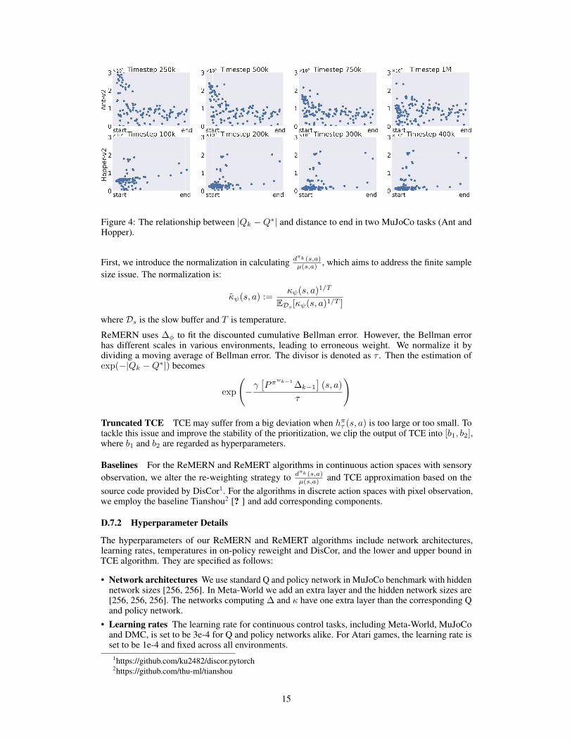
Figure 4: The relationship between |Qk −Q∗| and distance to end in two MuJoCo tasks (Ant andHopper).
First, we introduce the normalization in calculating dπk (s,a)µ(s,a) , which aims to address the finite sample
size issue. The normalization is:
κψ(s, a) :=κψ(s, a)1/T
EDs [κψ(s, a)1/T ]
where Ds is the slow buffer and T is temperature.
ReMERN uses ∆φ to fit the discounted cumulative Bellman error. However, the Bellman errorhas different scales in various environments, leading to erroneous weight. We normalize it bydividing a moving average of Bellman error. The divisor is denoted as τ . Then the estimation ofexp(−|Qk −Q∗|) becomes
exp
(−γ
[Pπ
wk−1∆k−1
](s, a)
τ
)
Truncated TCE TCE may suffer from a big deviation when hπτ (s, a) is too large or too small. Totackle this issue and improve the stability of the prioritization, we clip the output of TCE into [b1, b2],where b1 and b2 are regarded as hyperparameters.
Baselines For the ReMERN and ReMERT algorithms in continuous action spaces with sensoryobservation, we alter the re-weighting strategy to dπk (s,a)
µ(s,a) and TCE approximation based on thesource code provided by DisCor1. For the algorithms in discrete action spaces with pixel observation,we employ the baseline Tianshou2 [? ] and add corresponding components.
D.7.2 Hyperparameter Details
The hyperparameters of our ReMERN and ReMERT algorithms include network architectures,learning rates, temperatures in on-policy reweight and DisCor, and the lower and upper bound inTCE algorithm. They are specified as follows:
• Network architectures We use standard Q and policy network in MuJoCo benchmark with hiddennetwork sizes [256, 256]. In Meta-World we add an extra layer and the hidden network sizes are[256, 256, 256]. The networks computing ∆ and κ have one extra layer than the corresponding Qand policy network.
• Learning rates The learning rate for continuous control tasks, including Meta-World, MuJoCoand DMC, is set to be 3e-4 for Q and policy networks alike. For Atari games, the learning rate isset to be 1e-4 and fixed across all environments.
1https://github.com/ku2482/discor.pytorch2https://github.com/thu-ml/tianshou
15

• Temperatures The temperature for weights related with dπk (s,a)µ(s,a) is 7.5 and fixed across different
environments. Also, DisCor has a temperature hyperparameter related to the output normalizationof the error network. We keep it unchanged in the Meta-World and DMC benchmark, and divide itby 20 in MuJoCo environments to make it compatible with on-policy prioritization weights.
• Bounds in TCE We select time-adaptive lower and upper bounds for TCE. The lower bound risesfrom 0.4 when training begins to 0.9 when it ends, and the upper bound drops from 1.6 to 1.1accordingly. The bounds are fixed across different environments.
• Random Seeds In MuJoCo, Meta-World and DMC benchmarks, we run each experiment withfour random seeds. The results are plotted with the mean of the four experiments. In Atari games,we run experiments with three random seeds and select the one with max return.
16