regret bounds for the adaptive control of linear quadratic...

JMLR: Workshop and Conference Proceedings 19 (2011) 1–26 24th Annual Conference on Learning Theory

Regret Bounds for the Adaptive Control of Linear QuadraticSystems

Yasin Abbasi-Yadkori [email protected]

Csaba Szepesvari [email protected]

Department of Computing Science, University of Alberta

Editor: Sham Kakade, Ulrike von Luxburg

Abstract

We study the average cost Linear Quadratic (LQ) control problem with unknown modelparameters, also known as the adaptive control problem in the control community. Wedesign an algorithm and prove that apart from logarithmic factors its regret up to time Tis O(

√T ). Unlike previous approaches that use a forced-exploration scheme, we construct a

high-probability confidence set around the model parameters and design an algorithm thatplays optimistically with respect to this confidence set. The construction of the confidenceset is based on the recent results from online least-squares estimation and leads to improvedworst-case regret bound for the proposed algorithm. To the best of our knowledge this isthe the first time that a regret bound is derived for the LQ control problem.

1. Introduction

We study the average cost LQ control problem with unknown model parameters, also knownas the adaptive control problem in the control community. The problem is to minimize theaverage cost of a controller that operates in an environment whose dynamics is linear, whilethe cost is a quadratic function of the state and the control. The optimal solution is a linearfeedback controller which can be computed in a closed form from the matrices underlyingthe dynamics and the cost. In the learning problem, the topic of this paper, the dynamics ofthe environment is unknown. This problem is challenging since the control actions influenceboth the cost and the rate at which the dynamics is learned, a topic of adaptive control.The objective in this case is to minimize the regret of the controller, i.e. to minimize thedifference between the average cost incurred by the learning controller and that of theoptimal controller. In this paper, for the first time, we show an adaptive controller andprove that, under some assumptions, its expected regret is bounded by O(

√T ). We build

on recent works in online linear estimation and adaptive control design, the latter of whichwe survey next.

c© 2011 Y. Abbasi-Yadkori & C. Szepesvari.

Abbasi-Yadkori Szepesvari

When the model parameters are known and the state is fully observed, one can usethe principles of dynamic programming to obtain the optimal controller. The version ofthe problem that deals with the unknown model parameters is called the adaptive controlproblem. The early attempts to solve this problem relied on the certainty equivalence prin-ciple (Simon, 1956). The idea was to estimate the unknown parameters from observationsand then use the estimated parameters as if they were the true parameters to design acontroller. It was soon realized that the certainty equivalence principle does not necessarilyprovide enough information to reliably estimate the parameters and the estimated param-eters can converge to incorrect values with positive probability (Becker et al., 1985). Thisin turn might lead to suboptimal performance.

To avoid non-identification problem, methods that actively explore the environment togather information are developed (Lai and Wei, 1982a, 1987; Chen and Guo, 1987; Chenand Zhang, 1990; Fiechter, 1997; Lai and Ying, 2006; Campi and Kumar, 1998; Bittantiand Campi, 2006). However, only asymptotic results are proven for these methods. Oneexception is the work of Fiechter (1997) who proposes an algorithm for the “discounted”LQ problem and analyzes its performance in a PAC framework.

Most of the aforementioned methods use forced-exploration schemes to provide the suf-ficient exploratory information. The idea is to take exploratory actions according to a fixedand appropriately designed schedule. However, the forced-exploration schemes lack strongworst-case regret bounds, even in the simplest problems (see e.g. Dani and Hayes (2006),section 6). Unlike the preceding methods, Campi and Kumar (1998) proposes an algorithmthat uses the Optimism in the Face of Uncertainty (OFU) principle, which goes back to thework of Lai and Robbins (1985), to deal with the exploration/exploitation dilemma. Theycall this the Bet On the Best (BOB) principle. The idea is to construct high-probabilityconfidence sets around the model parameters, find the optimal controller for each memberof the confidence set, and finally choose the controller whose associated average cost is thesmallest. However, Campi and Kumar (1998) only show asymptotic optimality, i.e. theaverage cost of their algorithm converges to that of the optimal policy in the limit. In thispaper, we modify the algorithm and the proof technique of Campi and Kumar (1998) andextend their work to derive a finite time regret bound. Our work also builds upon on theworks of Lai and Wei (1982b); Dani et al. (2008); Rusmevichientong and Tsitsiklis (2010) inanalyzing the linear estimation with dependent covariates, although we use a more recent,improved confidence bound (see Theorem 1).

Note that the OFU principle has been applied very successfully to a number of challeng-ing learning and control situations. Lai and Robbins (1985), who invented the principle,used it to address learning in bandit problems (i.e., when there is no state) and later thiswork was picked up and modified by Auer et al. (2002) to make it work in nonparametricbandits. The OFU principle has also been applied to learning in finite Markov DecisionProcesses, both in a regret minimization (e.g., Bartlett and Tewari 2009; Auer et al. 2010)and in a PAC-learning setting (e.g., Kearns and Singh 1998; Brafman and Tennenholtz2002; Kakade 2003; Strehl et al. 2006; Szita and Szepesvari 2010). In the PAC-MDP frame-work there has been some work to extend the OFU principle to infinite Markov DecisionProblems under various assumptions. For example, Lipschitz assumptions have been used

2

Regret Bounds for the Adaptive Control of Linear Quadratic Systems

by Kakade et al. (2003), while Strehl and Littman (2008) explored linear models. However,none of these works consider both continuous state and action spaces. Continuous actionspaces in the context of bandits have been explored in a number of works, such as the worksof Kleinberg (2005); Auer et al. (2007); Kleinberg et al. (2008) and in a linear setting byAuer (2003); Dani et al. (2008) and Rusmevichientong and Tsitsiklis (2010).

2. Notation and conventions

We use ‖ · ‖ and ‖.‖F to denote the 2-norm and the Frobenius norm, respectively. For apositive semidefinite matrix A ∈ Rd×d, the weighted 2-norm ‖.‖A is defined by ‖x‖2A =x>Ax, where x ∈ Rd. The inner product is denoted by 〈·, ·〉. We use λmin(A) and λmax(A)to denote the minimum and maximum eigenvalues of the positive semidefinite matrix A,respectively. We use A 0 to denote that A is positive definite, while we use A 0 todenote that it is positive semidefinite. We use IA to denote the indicator function of eventA.

3. The Linear Quadratic Problem

We consider the discrete-time infinite-horizon linear quadratic (LQ) control problem:

xt+1 = A∗xt +B∗ut + wt+1,

ct = x>t Qxt + u>t Rut,

where t = 0, 1, . . . , ut ∈ Rd is the control at time t, xt ∈ Rn is the state at time t, ct ∈ R isthe cost at time t, wt+1 is the “noise”, A∗ ∈ Rn×n and B∗ ∈ Rn×d are unknown matriceswhile Q ∈ Rn×n and R ∈ Rd×d are known (positive definite) matrices. At time zero, forsimplicity, x0 = 0. The problem is to design a controller based on past observations tominimize the average expected cost

J(u0, u1, . . . ) = lim supT→∞

1

T

T∑t=0

E [ct] . (1)

Let J∗ be the optimal (lowest) average cost. The regret up to time T of a controller whichincurs a cost of ct at time t is defined by

R(T ) =T∑t=0

(ct − J∗) ,

which is the difference between the performance of the controller and the performance of theoptimal controller that has full information about the system dynamics. Thus the regretcan be interpreted as a measure of the cost of not knowing the system dynamics.

3


3.1. Assumptions

In this section, we state our assumptions on the noise and the system dynamics. In particu-lar, we assume that the noise is sub-Gaussian and the system is controllable and observable1.Define

Θ>∗ =(A∗ , B∗

)and zt =

(xtut

).

Thus, the state transition can be written as

xt+1 = Θ>∗ zt + wt+1 .

Assumption A1 There exists a filtration (Ft) such that for the random variables (z0, x1),. . ., (zt, xt+1), the following hold:

(i) zt, xt are Ft-measurable;

(ii) For any t ≥ 0,E [xt+1|Ft] = z>t Θ∗ ,

i.e., wt+1 = xt+1 − z>t θ∗ is a martingale difference sequence (E [wt+1|Ft] = 0, t =0, 1, . . .);

(iii) E[wt+1w

>t+1 | Ft

]= In;

(iv) The random variables wt are component-wise sub-Gaussian in the sense that thereexists L > 0 such that for any γ ∈ R, and index j,

E [exp(γwt+1,j)|Ft] ≤ exp(γ2L2/2) .

The assumption E[wt+1w

>t+1 | Ft

]= In makes the analysis more readable. However, we

shall show it in Section 4 that it is in fact not necessary. Our next assumption on thesystem uncertainty states that the unknown parameter is a member of a bounded set andis such that the system is controllable and observable. This assumption will let us derive aclosed form expression for the optimal control law.

Assumption A2 The unknown parameter Θ∗ is a member of set S such that

S ⊆ S0 ∩

Θ ∈ Rn×(n+d) | trace(Θ>Θ) ≤ S2,

where

S0 =

Θ = (A,B) ∈Rn×(n+d) | (A,B) is controllable,

(A,M) is observable, where Q = M>M.

In what follows, we shall always assume that the above assumptions are valid.

1. Controllability and observability are defined in Appendix B

4


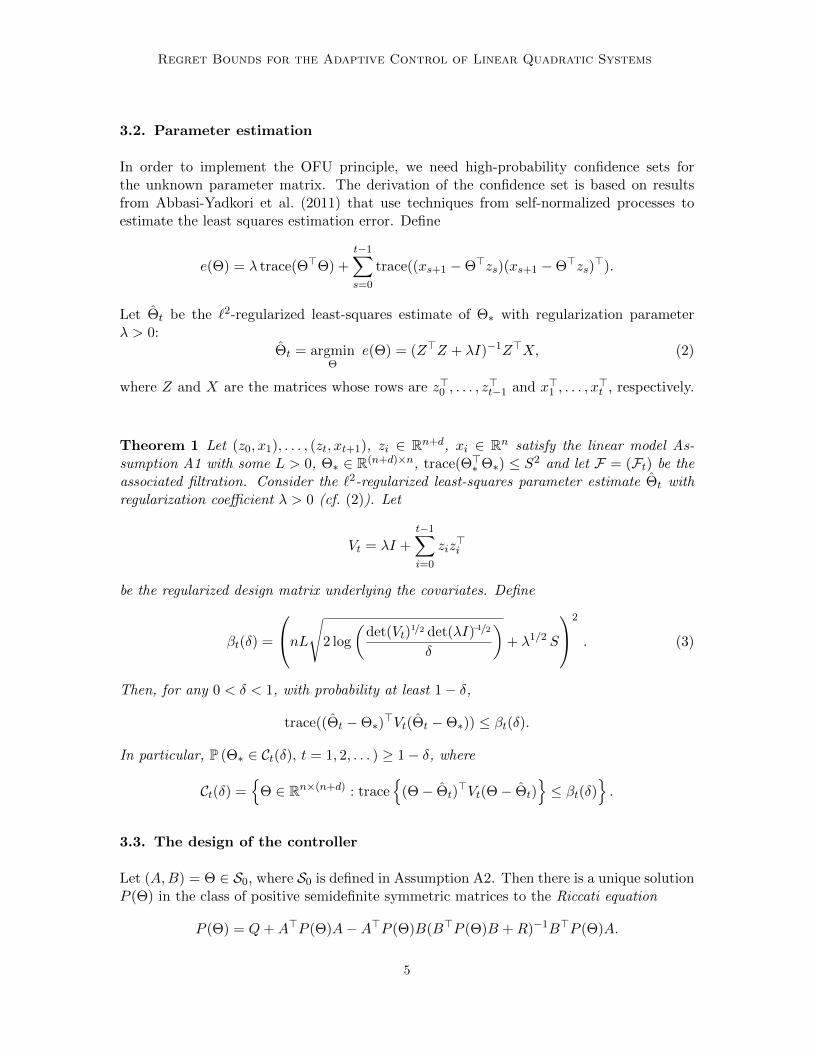
3.2. Parameter estimation

In order to implement the OFU principle, we need high-probability confidence sets forthe unknown parameter matrix. The derivation of the confidence set is based on resultsfrom Abbasi-Yadkori et al. (2011) that use techniques from self-normalized processes toestimate the least squares estimation error. Define

e(Θ) = λ trace(Θ>Θ) +

t−1∑s=0

trace((xs+1 −Θ>zs)(xs+1 −Θ>zs)>).

Let Θt be the `2-regularized least-squares estimate of Θ∗ with regularization parameterλ > 0:

Θt = argminΘ

e(Θ) = (Z>Z + λI)−1Z>X, (2)

where Z and X are the matrices whose rows are z>0 , . . . , z>t−1 and x>1 , . . . , x

>t , respectively.

Theorem 1 Let (z0, x1), . . . , (zt, xt+1), zi ∈ Rn+d, xi ∈ Rn satisfy the linear model As-sumption A1 with some L > 0, Θ∗ ∈ R(n+d)×n, trace(Θ>∗ Θ∗) ≤ S2 and let F = (Ft) be theassociated filtration. Consider the `2-regularized least-squares parameter estimate Θt withregularization coefficient λ > 0 (cf. (2)). Let

Vt = λI +t−1∑i=0

ziz>i

be the regularized design matrix underlying the covariates. Define

βt(δ) =

nL√2 log

(det(Vt)

1/2 det(λI)−1/2

δ

)+ λ1/2 S

2

. (3)

Then, for any 0 < δ < 1, with probability at least 1− δ,

trace((Θt −Θ∗)>Vt(Θt −Θ∗)) ≤ βt(δ).

In particular, P (Θ∗ ∈ Ct(δ), t = 1, 2, . . . ) ≥ 1− δ, where

Ct(δ) =

Θ ∈ Rn×(n+d) : trace

(Θ− Θt)>Vt(Θ− Θt)

≤ βt(δ)

.

3.3. The design of the controller

Let (A,B) = Θ ∈ S0, where S0 is defined in Assumption A2. Then there is a unique solutionP (Θ) in the class of positive semidefinite symmetric matrices to the Riccati equation

P (Θ) = Q+A>P (Θ)A−A>P (Θ)B(B>P (Θ)B +R)−1B>P (Θ)A.

5


Under the same assumptions, the matrix A+ BK(Θ) is stable, i.e. its norm-2 is less thanone, where

K(Θ) = −(B>P (Θ)B +R)−1B>P (Θ)A

is the gain matrix (Bertsekas, 2001). Further, by the boundedness of S, we also obtain theboundedness of P (Θ) (Anderson and Moore, 1971). The corresponding constant will bedenoted by D:

D = sup ‖P (Θ)‖ | Θ ∈ S . (4)

The optimal control law for a LQ system with parameters Θ is

ut = K(Θ)xt, (5)

i.e., this controller achieves the optimal average cost which satisfies J(Θ) = trace(P (Θ))(Bertsekas, 2001). In particular, the average cost of control law (5) with Θ = Θ∗ is theoptimal average cost J∗ = J(Θ∗) = trace(P (Θ∗)).

We assume that the bound on the norm of the unknown parameter, S, and the sub-Gaussianity constant, L, are known:

Assumption A3 Constants L and S in Assumptions A1 and A2 are known.

The algorithm that we propose implements the OFU principle as follows: At time t, thealgorithm chooses a parameter Θt from Ct(δ) ∩ S such that

J(Θt) ≤ infΘ∈Ct(δ)∩S

J(Θ) +1√t

and then uses the optimal feedback controller (5) underlying the chosen parameter. Inorder to prevent too frequent changes to the controller (which might harm performance),the algorithm changes controllers only after the current parameter estimates are significantlyrefined. The details of the algorithm are given in Algorithm 1.

4. Analysis

In this section we give our main result together with its proof. Before stating the maintheorem, we make one more assumption in addition to the assumptions we made before.

Assumption A4 The set S is such that ρ := sup(A,B)∈S ‖A+BK(A,B)‖ < 1. Further,there exists a positive number C such that C = supΘ∈S ‖K(Θ)‖ <∞.

Our main result is the following theorem:

6


Inputs: T, S > 0, δ > 0, Q, L, λ > 0.Set V0 = λI and Θ0 = 0.(A0, B0) = Θ0 = argminΘ∈C0(δ)∩S J(Θ).for t := 0, 1, 2, . . . do

if det(Vt) > 2 det(V0) thenCalculate Θt by (2).Find Θt such that J(Θt) ≤ infΘ∈Ct(δ)∩S J(Θ) + 1√

t.

Let V0 = Vt.else

Θt = Θt−1.end ifCalculate ut based on the current parameters, ut = K(Θt)xt.Execute control, observe new state xt+1.Save (zt, xt+1) into the dataset, where z>t = (x>t , u

>t ).

Vt+1 := Vt + ztz>t .

end for

Table 1: The proposed adaptive algorithm for the LQ problem

Theorem 2 For any 0 < δ < 1, for any time T , with probability at least 1 − δ, the regretof Algorithm 1 is bounded as follows:

R(T ) = O(√

T log(1/δ)),

where the constant hidden is a problem dependent constant.2

Remark 3 The assumption E[wt+1w

>t+1|Ft

]= In makes the analysis more readable. Alter-

natively, we could assume that E[wt+1w

>t+1|Ft

]= G∗ and G∗ be unknown. Then the optimal

average cost becomes J(Θ∗, G∗) = trace(P (Θ∗)G∗). The only change in Algorithm 1 is inthe computation of Θt, which will have the following form:

(Θt, G) = argmin(Θ,G)∈Ct

J(Θ),

where Ct is now a confidence set over Θ∗ and G∗. The rest of the analysis remains identical,provided that an appropriate confidence set is constructed.

The least squares estimation error from Theorem 1 scales with the size of the state andaction vectors. Thus, in order to prove Theorem 2, we first prove a high-probability boundon the norm of the state vector. Given the boundedness of the state, we decompose theregret and analyze each term using appropriate concentration inequalities.

2. Here, O hides logarithmic factors.

7


4.1. Bounding ‖xt‖

We choose an error probability, δ > 0. Given this, we define two “good events” in theprobability space Ω. In particular, we define the event that the confidence sets hold fors = 0, . . . , t,

Et = ω ∈ Ω : ∀s ≤ t, Θ∗ ∈ Cs(δ/4) ,

and the event that the state vector stays “small”:

Ft = ω ∈ Ω : ∀s ≤ t, ‖xs‖ ≤ αt

where

αt =1

1− ρ

(η

ρ

)n+d[GZ

n+dn+d+1

T βt(δ/4)1

2(n+d+1) + 2L

√n log

4nt(t+ 1)

δ

],

η = 1 ∨ supΘ∈S‖A∗ +B∗K(Θ)‖ ,

ZT = max0≤t≤T

‖zt‖ ,

G = 2

(2S(n+ d)n+d+1/2

U1/2

)1/(n+d+1)

,

U =U0

H,

U0 =1

16n+d−2(1 ∨ S2(n+d−2)),

and H is any number satisfying3

H >

(16 ∨ 4S2M2

(n+ d)U0

),

where

M = supY≥0

(nL

√(n+ d) log

(1+TY/λ

δ

)+ λ1/2S

)Y

.

In what follows, we let E = ET and F = FT . First, we show that E ∩ F holds with highprobability and on E ∩ F , the state vector does not explode.

Lemma 4 P (E ∩ F ) ≥ 1− δ/2.

The proof is in Appendix D. It first shows that∥∥∥(Θ∗ − Θt)

>zt

∥∥∥ is well controlled except

for a small number of occasions. Given this and proper decomposition of the state updateequation, we can prove that the state vector xt stays smaller than αt. Notice that αt itselfdepends βt and ZT , which in turn depend on xt. Thus, we need one more step to have abound on ‖xt‖.

3. We use ∧ and ∨ to denote the minimum and the maximum, respectively.

8


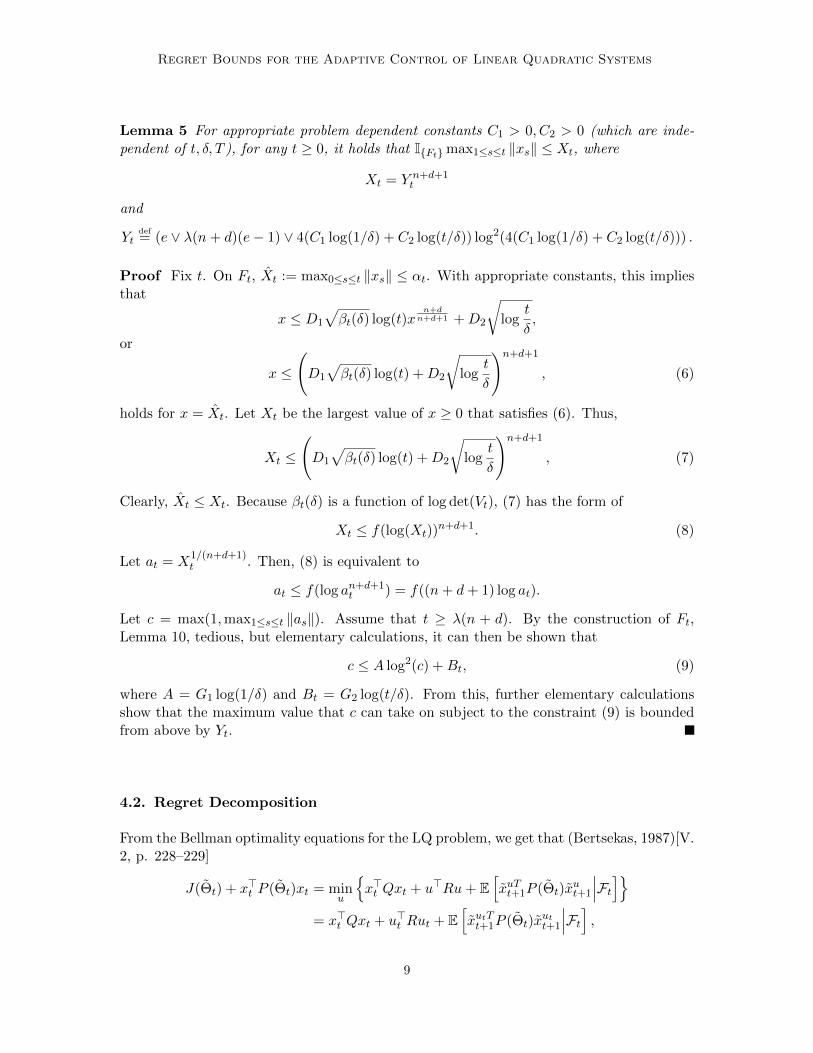
Lemma 5 For appropriate problem dependent constants C1 > 0, C2 > 0 (which are inde-pendent of t, δ, T ), for any t ≥ 0, it holds that IFtmax1≤s≤t ‖xs‖ ≤ Xt, where

Xt = Y n+d+1t

and

Ytdef= (e ∨ λ(n+ d)(e− 1) ∨ 4(C1 log(1/δ) + C2 log(t/δ)) log2(4(C1 log(1/δ) + C2 log(t/δ))) .

Proof Fix t. On Ft, Xt := max0≤s≤t ‖xs‖ ≤ αt. With appropriate constants, this impliesthat

x ≤ D1

√βt(δ) log(t)x

n+dn+d+1 +D2

√log

t

δ,

or

x ≤

(D1

√βt(δ) log(t) +D2

√log

t

δ

)n+d+1

, (6)

holds for x = Xt. Let Xt be the largest value of x ≥ 0 that satisfies (6). Thus,

Xt ≤

(D1

√βt(δ) log(t) +D2

√log

t

δ

)n+d+1

, (7)

Clearly, Xt ≤ Xt. Because βt(δ) is a function of log det(Vt), (7) has the form of

Xt ≤ f(log(Xt))n+d+1. (8)

Let at = X1/(n+d+1)t . Then, (8) is equivalent to

at ≤ f(log an+d+1t ) = f((n+ d+ 1) log at).

Let c = max(1,max1≤s≤t ‖as‖). Assume that t ≥ λ(n + d). By the construction of Ft,Lemma 10, tedious, but elementary calculations, it can then be shown that

c ≤ A log2(c) +Bt, (9)

where A = G1 log(1/δ) and Bt = G2 log(t/δ). From this, further elementary calculationsshow that the maximum value that c can take on subject to the constraint (9) is boundedfrom above by Yt.

4.2. Regret Decomposition

From the Bellman optimality equations for the LQ problem, we get that (Bertsekas, 1987)[V.2, p. 228–229]

J(Θt) + x>t P (Θt)xt = minu

x>t Qxt + u>Ru+ E

[xuTt+1P (Θt)x

ut+1

∣∣∣Ft]= x>t Qxt + u>t Rut + E

[xutTt+1P (Θt)x

utt+1

∣∣∣Ft] ,9


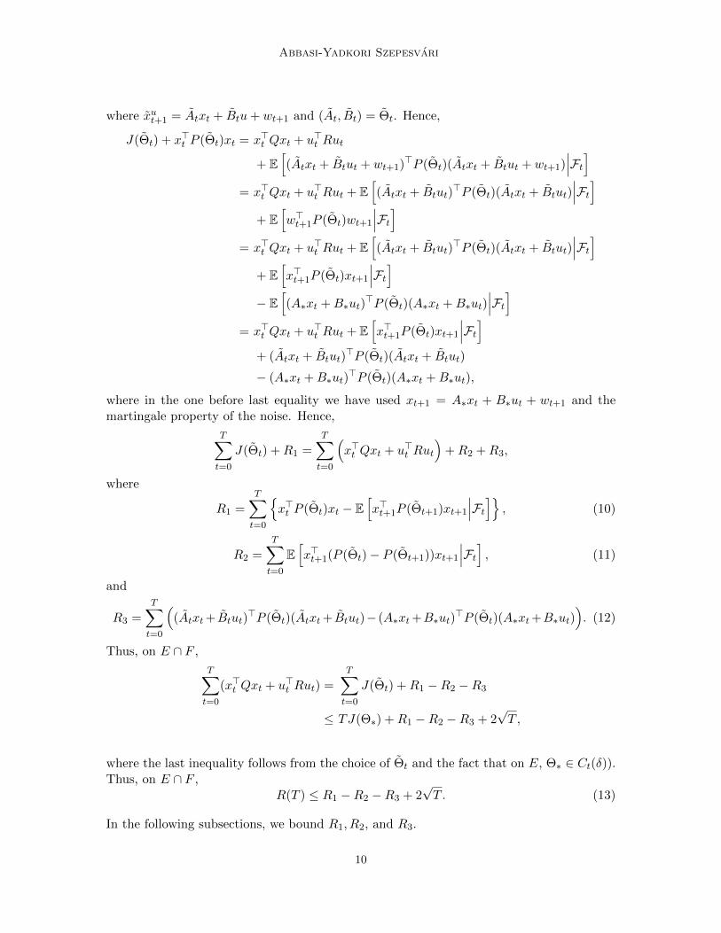
where xut+1 = Atxt + Btu+ wt+1 and (At, Bt) = Θt. Hence,

J(Θt) + x>t P (Θt)xt = x>t Qxt + u>t Rut

+ E[(Atxt + Btut + wt+1)>P (Θt)(Atxt + Btut + wt+1)


[(Atxt + Btut)

>P (Θt)(Atxt + Btut)∣∣∣Ft]

+ E[w>t+1P (Θt)wt+1


[(Atxt + Btut)

>P (Θt)(Atxt + Btut)∣∣∣Ft]

+ E[x>t+1P (Θt)xt+1

∣∣∣Ft]− E

[(A∗xt +B∗ut)

>P (Θt)(A∗xt +B∗ut)∣∣∣Ft]

= x>t Qxt + u>t Rut + E[x>t+1P (Θt)xt+1

∣∣∣Ft]+ (Atxt + Btut)

>P (Θt)(Atxt + Btut)

− (A∗xt +B∗ut)>P (Θt)(A∗xt +B∗ut),

where in the one before last equality we have used xt+1 = A∗xt + B∗ut + wt+1 and themartingale property of the noise. Hence,

T∑t=0

J(Θt) +R1 =T∑t=0

(x>t Qxt + u>t Rut

)+R2 +R3,

where

R1 =T∑t=0

x>t P (Θt)xt − E

[x>t+1P (Θt+1)xt+1

∣∣∣Ft] , (10)

R2 =

T∑t=0

E[x>t+1(P (Θt)− P (Θt+1))xt+1

∣∣∣Ft] , (11)

and

R3 =

T∑t=0

((Atxt+ Btut)

>P (Θt)(Atxt+ Btut)− (A∗xt+B∗ut)>P (Θt)(A∗xt+B∗ut)

). (12)

Thus, on E ∩ F ,

T∑t=0

(x>t Qxt + u>t Rut) =T∑t=0

J(Θt) +R1 −R2 −R3

≤ TJ(Θ∗) +R1 −R2 −R3 + 2√T ,

where the last inequality follows from the choice of Θt and the fact that on E, Θ∗ ∈ Ct(δ)).Thus, on E ∩ F ,

R(T ) ≤ R1 −R2 −R3 + 2√T . (13)

In the following subsections, we bound R1, R2, and R3.

10


4.3. Bounding IE∩FR1

We start by showing that with high probability all noise terms are small.

Lemma 6 With probability 1− δ/8, for any k ≤ T , ‖wk‖ ≤ Ln√

2n log(8nT/δ).

Proof From sub-Gaussianity Assumption A1, we have that for any index 1 ≤ i ≤ n andany time k,

|wk,i| ≤ L√

2 log(8/δ) .

Thus, with probability 1− δ/8, for any k ≤ T , ‖wk‖ ≤ Ln√

2n log(8nT/δ).

Lemma 7 Let R1 be as defined by (10). With probability at least 1− δ/2,

IE∩FR1 ≤ 2DW 2

√2T log

8

δ+ n

√B′δ,

where W = Ln√

2n log(8nT/δ) and

B′δ =(v + TD2S2X2(1 + C2)

)log

(4nv−1/2

δ

(v + TD2S2X2(1 + C2)

)1/2).

Proof Let ft−1 = A∗xt−1 +B∗ut−1 and Pt = P (Θt). Write

R1 = x>0 P (Θ0)x0 − x>T+1P (ΘT+1)xT+1

+T∑t=1

(x>t P (Θt)xt − E

[x>t P (Θt)xt|Ft−1

] ).

Because P is positive semi-definite and x0 = 0, the first term is bounded by zero. Thesecond term can be decomposed as follows

T∑t=1

(x>t Ptxt − E

[x>t Ptxt|Ft−1

] )=

T∑t=1

f>t−1Ptwt

+

T∑t=1

(w>t Ptwt − E

[w>t Ptwt|Ft−1

] ).

We bound each term separately. Let v>t = f>t−1Pt and

G1 = IE∩FT∑t=1

v>t wt = IE∩FT∑t=1

n∑i=1

vk,iwk,i =n∑i=1

IE∩FT∑t=1

vk,iwk,i.

11


Let MT,i =∑T

t=1 vk,iwk,i. By Theorem 16, on some event Gδ,i that holds with probabilityat least 1− δ/(4n), for any T ≥ 0,

M2T,i ≤ 2R2

(v +

T∑t=1

v2t,i

)log

4nv−1/2

δ

(v +

T∑t=1

v2t,i

)1/2 = Bδ,i.

On E∩F , ‖vt‖ ≤ DSX√

1 + C2 and thus, vt,i ≤ DSX√

1 + C2. Thus, onGδ,i, IE∩FM2t,i ≤

B′δ. Thus, we have G1 ≤∑n

i=1

√B′δ,i on ∩ni=1Gδ,i, that holds w.p. 1− δ/4.

Define Xt = w>t Ptwt −E[w>t Ptwt|Ft−1

]and its truncated version Xt = XtIXt≤2DW 2.

Define G2 =∑T

t=1Xt and G2 =∑T

t=1 Xt. By Lemma 14,

P

(G2 > 2DW 2

√2T log

8

δ

)≤ P

(max

1≤t≤TXt ≥ 2DW 2

)+ P

(G2 > 2DW 2

√2T log

8

δ

).

By Lemma 6 and Azuma’s inequality, each term on the right hand side is bounded by δ/8.Thus, w.p. 1− δ/4,

G2 ≤ 2DW 2

√2T log

8

δ

Summing up the bounds on G1 and G2 gives the result that holds w.p. at least 1− δ/2,

IE∩FR1 ≤ 2DW 2

√2T log

8

δ+ n

√B′δ.

4.4. Bounding IE∩F |R2|

We can bound IE∩F |R2| by simply showing that Algorithm 1 rarely changes the policy,and hence most terms in (11) are zero.

Lemma 8 On the event E ∩ F , Algorithm 1 changes the policy at most

(n+ d) log2

(1 + TX2

T (1 + C2)/λ)

times up to time T .

Proof If we have changed the policy K times up to time T , then we should have thatdet(VT ) ≥ λn+d2K . On the other hand, we have

λmax(VT ) ≤ λ+

T−1∑t=0

‖zt‖2 ≤ λ+ TX2T (1 + C2),

12


where C is the bound on the norm of K(.) as defined in Assumption A4. Thus, it holdsthat

λn+d2K ≤ (λ+ TX2T (1 + C2))n+d.

Solving for K, we get

K ≤ (n+ d) log2

(1 +

TX2T (1 + C2)

λ

).

Lemma 9 Let R2 be as defined by Equation (11). Then we have

IE∩F |R2| ≤ 2DX2T (n+ d) log2

(1 + TX2

T (1 + C2)/λ).

Proof On event E ∩ F , we have at most K = (n + d) log2

(1 + TX2

T (1 + C2)/λ)

policychanges up to time T . So at most K terms in the summation (11) are non-zero. Each termin the summation is bounded by 2DX2

T . Thus,

IE∩F |R2| ≤ 2DX2T (n+ d) log2

(1 + TX2

T (1 + C2)/λ).

4.5. Bounding IE∩F |R3|

The summation∑T

t=0

∥∥∥(Θ∗ − Θt)>zt

∥∥∥2will appear in the analysis while bounding |R3|. So

we first bound this summation, whose analysis requires the following two results.

Lemma 10 The following holds for any t ≥ 1:

t−1∑k=0

(‖zk‖2V −1

k∧ 1)≤ 2 log

det(Vt)

det(λI).

Further, when the covariates satisfy ‖zt‖ ≤ cm, t ≥ 0 with some cm > 0 w.p.1 then

logdet(Vt)

det(λI)≤ (n+ d) log

(λ(n+ d) + tc2

m

λ(n+ d)

).

The proof of the lemma can be found in Abbasi-Yadkori et al. (2011).

Lemma 11 Let A ∈ Rm×m and B ∈ Rm×m be positive semi-definite matrices such thatA B. Then, we have

supX 6=0

∥∥X>AX∥∥‖X>BX‖

≤ det(A)

det(B).

13


The proof of this lemma is in Appendix C.

Lemma 12 On E ∩ F , it holds that

T∑t=0

∥∥∥(Θ∗ − Θt)>zt

∥∥∥2≤ 16

λ(1 + C2)X2

TβT (δ/4) logdet(VT )

det(λI).

Proof Consider timestep t. Let st = (Θ∗ − Θt)>zt. Let τ ≤ t be the last timestep when

the policy is changed. So st = (Θ∗ − Θτ )>zt. We have

‖st‖ ≤∥∥∥(Θ∗ − Θτ )>zt

∥∥∥+∥∥∥(Θτ − Θτ )>zt

∥∥∥ . (14)

For all Θ ∈ Cτ ,∥∥∥(Θ− Θτ )>zt

∥∥∥ ≤ ∥∥∥V 1/2t (Θ− Θτ )

∥∥∥ ‖zt‖V −1t

(Cauchy-Schwartz inequality)

≤∥∥∥V 1/2

τ (Θ− Θτ )∥∥∥√ det(Vt)

det(Vτ )‖zt‖V −1

t(Lemma 11)

≤√

2∥∥∥V 1/2

τ (Θ− Θτ )∥∥∥ ‖zt‖V −1

t(Choice of τ)

≤√

2βτ (δ/4) ‖zt‖V −1t, (λmax(M) ≤ trace(M) for M 0)

Applying the last inequality to Θ∗ and Θτ , together with (14) gives

‖st‖2 ≤ 8βτ (δ/4) ‖zt‖2V −1t.

Now, by Assumption A4 and the fact that Θt ∈ S we have that

‖zt‖2V −1t≤ ‖zt‖

2

λ≤

(1 + C2)X2T

λ.

It follows then that

T∑t=0

‖st‖2 ≤8

λ(1 + C2)X2

TβT (δ/4)T∑t=0

(‖zt‖2V −1t∧ 1)

≤ 16

λ(1 + C2)X2

TβT (δ/4) logdet(VT )

det(λI). (Lemma 10).

Now, we are ready to bound R3.

Lemma 13 Let R3 be as defined by Equation (12). Then we have

IE∩F |R3| ≤8√λ

(1 + C2)X2TSD

(βT (δ/4) log

det(VT )

det(λI)

)1/2√T .

14


Proof We have that

IE∩F |R3| ≤ IE∩FT∑t=0

∣∣∣∣∥∥∥P (Θt)1/2Θ>t zt

∥∥∥2−∥∥∥P (Θt)

1/2Θ>∗ zt

∥∥∥2∣∣∣∣ (Tri. ineq.)

≤ IE∩F

(T∑t=0

(∥∥∥P (Θt)1/2Θ>t zt

∥∥∥− ∥∥∥P (Θt)1/2Θ>∗ zt

∥∥∥)2)1/2

(C.-S. ineq.)

×

(T∑t=0

(∥∥∥P (Θt)1/2Θ>t zt

∥∥∥+∥∥∥P (Θt)

1/2Θ>∗ zt

∥∥∥)2)1/2

≤ IE∩F

(T∑t=0

∥∥∥P (Θt)1/2(Θt −Θ∗)

>zt

∥∥∥2)1/2

(Tri. ineq.)

×

(T∑t=0

(∥∥∥P (Θt)1/2Θ>t zt

∥∥∥+∥∥∥P (Θt)

1/2Θ>∗ zt

∥∥∥)2)1/2

≤ 8√λ

(1 + C2)X2TSD

(βT (δ/4) log

det(VT )

det(λI)

)1/2√T . ((4), L. 12)

Now we are ready to prove Theorem 2.

4.6. Putting Everything Together

Proof [Proof of Theorem 2] By (13) and Lemmas 7, 9, 13 we have that with probability atleast 1− δ/2,

IE∩F(R1 −R2 −R3) ≤ 2DX2T (n+ d) log2

(1 + TX2

T (1 + C2)/λ)

+ 2DW 2

√2T log

8

δ+ n

√B′δ

+8√λ

(1 + C2)X2TSD

(βT (δ/4) log

det(VT )

det(λI)

)1/2√T .

Thus, on E ∩ F , with probability at least 1− δ/2,

R(T ) ≤ 2DX2T (n+ d) log2

(1 + TX2

T (1 + C2)/λ)

+ 2DW 2

√2T log

8

δ+ n

√B′δ

+8√λ

(1 + C2)X2TSD

(βT (δ/4) log

det(VT )

det(λI)

)1/2√T .

Further, on E ∩ F , by Lemmas 5 and 10,

log detVT ≤ (n+ d) log

(λ(n+ d) + T (1 + C2)X2

T

λ(n+ d)

)+ log detλI.

15


Plugging in this gives the final bound, which, by Lemma 4, holds with probability 1− δ.

References

Y. Abbasi-Yadkori, D. Pal, and Cs. Szepesvari. Online least squares estimationwith self-normalized processes: An application to bandit problems. Arxiv preprinthttp://arxiv.org/abs/1102.2670, 2011.

B. D. O. Anderson and J. B. Moore. Linear Optimal Control. Prentice-Hall, 1971.

P. Auer. Using confidence bounds for exploitation-exploration trade-offs. Journal of Ma-chine Learning Research, 3:397–422, 2003. ISSN 1533-7928.

P. Auer, N. Cesa-Bianchi, and P. Fischer. Finite time analysis of the multiarmed banditproblem. Machine Learning, 47(2-3):235–256, 2002.

P. Auer, R. Ortner, and Cs. Szepesvari. Improved rates for the stochastic continuum-armed bandit problem. In Proceedings of the 20th Annual Conference on Learning Theory(COLT-07), pages 454–468, 2007.

P. Auer, T. Jaksch, and R. Ortner. Near-optimal regret bounds for reinforcement learning.Journal of Machine Learning Research, 11:1563—1600, 2010.

P. L. Bartlett and A. Tewari. REGAL: A regularization based algorithm for reinforcementlearning in weakly communicating MDPs. In Proceedings of the 25th Annual Conferenceon Uncertainty in Artificial Intelligence, 2009.

A. Becker, P. R. Kumar, and C. Z. Wei. Adaptive control with the stochastic approximationalgorithm: Geometry and convergence. IEEE Trans. on Automatic Control, 30(4):330–338, 1985.

D. Bertsekas. Dynamic Programming. Prentice-Hall, 1987.

D. P. Bertsekas. Dynamic Programming and Optimal Control. Athena Scientific, 2nd edition,2001.

S. Bittanti and M. C. Campi. Adaptive control of linear time invariant systems: the “beton the best” principle. Communications in Information and Systems, 6(4):299–320, 2006.

R. I. Brafman and M. Tennenholtz. R-MAX - a general polynomial time algorithm fornear-optimal reinforcement learning. Journal of Machine Learning Research, 3:213–231,2002.

M. C. Campi and P. R. Kumar. Adaptive linear quadratic Gaussian control: the cost-biasedapproach revisited. SIAM Journal on Control and Optimization, 36(6):1890–1907, 1998.

H. Chen and L. Guo. Optimal adaptive control and consistent parameter estimates forarmax model with quadratic cost. SIAM Journal on Control and Optimization, 25(4):845–867, 1987.

16


H. Chen and J. Zhang. Identification and adaptive control for systems with unknown orders,delay, and coefficients. Automatic Control, IEEE Transactions on, 35(8):866 –877, August1990.

V. Dani and T. P. Hayes. Robbing the bandit: Less regret in online geometric optimiza-tion against an adaptive adversary. In 16th Annual ACM-SIAM Symposium on DiscreteAlgorithms, pages 937–943, 2006.

V. Dani, T. P. Hayes, and S. M. Kakade. Stochastic linear optimization under banditfeedback. COLT-2008, pages 355–366, 2008.

C. Fiechter. Pac adaptive control of linear systems. In in Proceedings of the 10th AnnualConference on Computational Learning Theory, ACM, pages 72–80. Press, 1997.

S. M. Kakade. On the sample complexity of reinforcement learning. PhD thesis, GatsbyComputational Neuroscience Unit, University College London, 2003.

S. M. Kakade, M. J. Kearns, and J. Langford. Exploration in metric state spaces. InT. Fawcett and N. Mishra, editors, ICML 2003, pages 306–312. AAAI Press, 2003.

M. Kearns and S. P. Singh. Near-optimal performance for reinforcement learning in poly-nomial time. In J. W. Shavlik, editor, ICML 1998, pages 260–268. Morgan Kauffmann,1998.

R. Kleinberg. Nearly tight bounds for the continuum-armed bandit problem. In Advancesin Neural Information Processing Systems, pages 697–704, 2005.

R. Kleinberg, A. Slivkins, and E. Upfal. Multi-armed bandits in metric spaces. In Pro-ceedings of the 40th annual ACM symposium on Theory of computing, pages 681–690,2008.

T. L. Lai and H. Robbins. Asymptotically efficient adaptive allocation rules. Advances inApplied Mathematics, 6:4–22, 1985.

T. L. Lai and C. Z. Wei. Least squares estimates in stochastic regression models withapplications to identification and control of dynamic systems. The Annals of Statistics,10(1):pp. 154–166, 1982a.

T. L. Lai and C. Z. Wei. Least squares estimates in stochastic regression models withapplications to identification and control of dynamic systems. The Annals of Statistics,10(1):154–166, 1982b.

T. L. Lai and C. Z. Wei. Asymptotically efficient self-tuning regulators. SIAM Journal onControl and Optimization, 25:466–481, March 1987.

T. L. Lai and Z. Ying. Efficient recursive estimation and adaptive control in stochasticregression and armax models. Statistica Sinica, 16:741–772, 2006.

P. Rusmevichientong and J. N. Tsitsiklis. Linearly parameterized bandits. Mathematics ofOperations Research, 35(2):395–411, 2010.

17


H. A. Simon. dynamic programming under uncertainty with a quadratic criterion function.Econometrica, 24(1):74–81, 1956.

A. L. Strehl and M. L. Littman. Online linear regression and its application to model-basedreinforcement learning. In NIPS, pages 1417–1424, 2008.

A. L. Strehl, L. Li, E. Wiewiora, J. Langford, and M. L. Littman. PAC model-free rein-forcement learning. In ICML, pages 881–888, 2006.

I. Szita and Cs. Szepesvari. Model-based reinforcement learning with nearly tight explo-ration complexity bounds. In ICML 2010, pages 1031–1038, 2010.

Appendix A. Tools from Probability Theorem

Lemma 14 Let X1, . . . , Xt be random variables. Let a ∈ R. Let St =∑t

s=1Xs andSt =

∑ts=1XsIXs≤a. Then it holds that

P (St > x) ≤ P(

max1≤s≤t

Xs ≥ a)

+ P(St > x

).

Proof

P (St ≥ x) ≤ P(

max1≤s≤t

Xs ≥ a)

+ P(St ≥ x, max

1≤s≤tXs ≤ a

)≤ P

(max1≤s≤t

Xs ≥ a)

+ P(St ≥ x

).

Theorem 15 (Azuma’s inequality) Assume that (Xs; s ≥ 0) is a supermartingale and|Xs −Xs−1| ≤ cs almost surely. Then for all t > 0 and all ε > 0,

P (|Xt −X0| ≥ ε) ≤ 2 exp

(−ε2

2∑t

s=1 c2s

).

Theorem 16 (Self-normalized bound for vector-valued martingales) Let (Fk; k ≥0) be a filtration, (mk; k ≥ 0) be an Rd-valued stochastic process adapted to (Fk), (ηk; k ≥ 1)be a real-valued martingale difference process adapted to (Fk). Assume that ηk is condition-ally sub-Gaussian with constant R. Consider the martingale

St =

t∑k=1

ηkmk−1

18


and the matrix-valued processes

Vt =t∑

k=1

mk−1m>k−1, V t = V + Vt, t ≥ 0,

Then for any 0 < δ < 1, with probability 1− δ,

∀t ≥ 0, ‖St‖2V −1t≤ 2R2 log

(det(V t)

1/2 det(V )−1/2

δ

).

Appendix B. Controllability and Observability

Definition 1 (Bertsekas (2001)) A pair (A,B), where A is an n × n matrix and B isan n× d matrix, is said to be controllable if the n× nd matrix

[B AB . . . An−1B]

has full rank. A pair (A,C), where A is an n× n matrix and C is an d× n matrix, is saidto be observable if the pair (A>, C>) is controllable.

Appendix C. Proof of Lemma 11

Proof [Proof of Lemma 11]

We consider first a simple case. Let A = B + mm>, B positive definite. Let X 6= 0be an arbitrary matrix. Using the Cauchy-Schwartz inequality and the fact that for anymatrix M ,

∥∥M>M∥∥ = ‖M‖2, we get∥∥∥X>mm>X∥∥∥ =∥∥∥m>X∥∥∥2

=∥∥∥m>B−1/2B1/2X

∥∥∥2≤∥∥∥m>B−1/2

∥∥∥2 ∥∥∥B1/2X∥∥∥2.

Thus, ∥∥∥X>(B +mm>)X∥∥∥ ≤ ∥∥∥X>BX∥∥∥+

∥∥∥m>B−1/2∥∥∥2 ∥∥∥B1/2X

∥∥∥2

=

(1 +

∥∥∥m>B−1/2∥∥∥2)∥∥∥B1/2X

∥∥∥2

and so ∥∥X>AX∥∥‖X>BX‖

≤ 1 +∥∥∥m>B−1/2

∥∥∥2.

We also have that

det(A) = det(B +mm>) = det(B) det(I +B−1/2m(B−1/2m)>) = det(B)(1 + ‖m‖2B−1),

thus finishing the proof of this case.

19


More generally, if A = B+m1m>1 + · · ·+mt−1m

>t−1 then define Vs = B+m1m

>1 + · · ·+

ms−1m>s−1 and use∥∥X>AX∥∥

‖X>BX‖=

∥∥X>VtX∥∥‖X>Vt−1X‖

∥∥X>Vt−1X∥∥

‖X>Vt−2X‖. . .

∥∥X>V2X∥∥

‖X>BX‖.

By the above argument, since all the terms are positive, we get∥∥X>AX∥∥‖X>BX‖

≤ det(Vt)

det(Vt−1)

det(Vt−1)

det(Vt−2). . .

det(V2)

det(B)=

det(Vt)

det(B)=

det(A)

det(B),

the desired inequality.

Finally, by SVD, if C 0, C can be written as the sum of at most m rank-one matrices,finishing the proof for the general case.

Appendix D. Bounding ‖xt‖

We show that E ∩ F holds with high probability.

Proof [Proof of Lemma 4] Let Mt = Θ∗ − Θt. On event E, for any t ≤ T we have that

trace

(M>t

(t−1∑s=0

λI + zsz>s

)Mt

)≤ βt(δ/4).

Since λ > 0 we get that,

trace

(t−1∑s=0

M>t zsz>s Mt

)≤ βt(δ/4).

Thus,t−1∑s=0

trace(M>t zsz>s Mt) ≤ βt(δ/4).

Since λmax(M) ≤ trace(M) for M 0, we get that

t−1∑s=0

∥∥∥M>t zs∥∥∥2≤ βt(δ/4).

Thus, for all t ≥ 1,

max0≤s≤t−1

∥∥∥M>t zs∥∥∥ ≤ βt(δ/4)1/2 ≤ βT (δ/4)1/2. (15)

Choose

H >

(16 ∨ 4S2M2

(n+ d)U0

),

20


where

U0 =1

16n+d−2(1 ∨ S2(n+d−2)),

and

M = supY≥0

(nL

√(n+ d) log

(1+TY/λ

δ

)+ λ1/2S

)Y

.

Fix a real number 0 ≤ ε ≤ 1, and consider the time horizon T . Let π(v,B) and π(M,B) bethe projections of vector v and matrix M onto subspace B ⊂ R(n+d), where the projectionof matrix M is done column-wise. Let B ⊕ v be the span of B and v. Let B⊥ be thesubspace orthogonal to B such that R(n+d) = B ⊕ B⊥.

Define a sequence of subspaces Bt as follows: Set BT+1 = ∅. For t = T, . . . , 1, initializeBt = Bt+1. Then while

∥∥π(Mt,B⊥t )∥∥F> (n + d)ε, choose a column of Mt, v, such that∥∥π(v,B⊥t )

∥∥F> ε and update Bt = Bt ⊕ v. After finishing with timestep t, we will have∥∥∥π(Mt,B⊥t )

∥∥∥ ≤ ∥∥∥π(Mt,B⊥t )∥∥∥F≤ (n+ d)ε. (16)

Let TT be the set of timesteps at which subspace Bt expands. The cardinality of this set,m, is at most n+ d. Denote these timesteps by t1 > t2 > · · · > tm. Let i(t) = max1 ≤ i ≤m : ti ≥ t.

Lemma 17 For any vector x ∈ Rn+d

Uε2(n+d) ‖π(x,Bt)‖2 ≤i(t)∑i=1

∥∥∥M>ti x∥∥∥2,

where U = U0/H.

Proof Let N = v1, . . . , vm be the set of vectors that are added to Bt during the expansiontimesteps. By construction, N is a subset of the set of all columns of Mt1 ,Mt2 , . . . ,Mti(t) .Thus, we have that

i(t)∑i=1

∥∥∥M>ti x∥∥∥2≥ x>(v1v

>1 + · · ·+ vmv

>m)x.

Thus, in order to prove the statement of the lemma, it is enough to show that

∀x, ∀j ∈ 1, . . . ,m,j∑

k=1

〈vk, x〉2 ≥ε4

H

ε2(j−2)

16j−2(1 ∨ S2(j−2))‖π(x,Bj)‖2 , (17)

where Bj = span(v1, . . . , vj) for any 1 ≤ j ≤ m. We have Bm = Bt. We can writevk = wk + uk, where wk ∈ Bk−1, uk ⊥ Bk−1, ‖uk‖ ≥ ε, and ‖vk‖ ≤ 2S.

The inequality (17) is proven by induction. First, we prove the induction base for j = 1.Without loss of generality, assume that x = Cv1. From condition H > 16, we get that

16−1H(1 ∨ S−1) ≥ 1.

21


B

P

L

α

β

v

η

x

λ

Figure 1: The geometry used in the inductive step. v = vl+1 and B = Bl.

Thus,

ε2 ≥ ε2

16−1H(1 ∨ S−1).

Thus,

C2 ‖v1‖4 ≥ε2C2 ‖v1‖2

16−1H(1 ∨ S−1),

where we have used the fact that ‖v1‖ ≥ ε. Thus,

〈v1, x〉2 ≥ε4

H

ε−2

16−1(1 ∨ S−2)‖π(x,B1)‖2 ,

which establishes the base of induction.

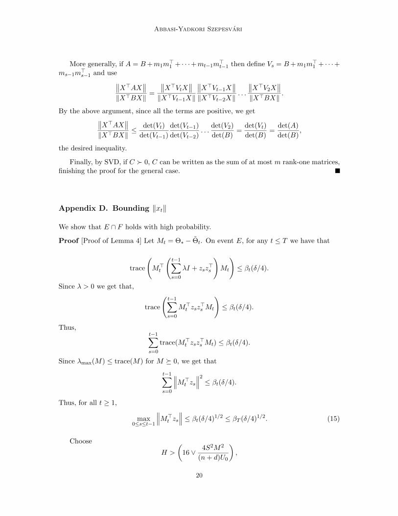
Next, we prove that if the inequality (17) holds for j = l, then it also holds for j = l+1.Figure 1 contains all relevant quantities that are used in the following argument.

Assume that the inequality (17) holds for j = l. Without loss of generality, assume thatx is in Bl+1, and thus ‖x‖ = ‖π(x,Bl+1)‖. Let P ⊂ Bl+1 be the 2-dimensional subspace thatpasses through x and vl+1. The 2-dimensional subspace P and the l-dimensional subspaceBl can, respectively, be identified by l − 1 and one equations in Bl+1. Because P is not asubset of Bl, the intersection of P and Bl is a line in Bl+1. Let’s call this line L. The lineL creates two half-planes on P . Without loss of generality, assume that x and vl+1 are onthe same half-plane (notice that we can always replace x by −x in (17)).

Let 0 ≤ β ≤ π/2 be the angle between vl+1 and L. Let 0 < λ < π/2 be the orthogonalangle between vl+1 and Bl. We know that β > λ, ul+1 is orthogonal to Bl, and ‖ul+1‖ ≥ ε.Thus, β ≥ arcsin(ε/ ‖vl+1‖). Let 0 ≤ α ≤ π be the angle between x and L (α < π, becausex and vl+1 are on the same half-plane). The direction of α is chosen so that it is consistentwith the direction of β. Finally, let 0 ≤ η ≤ π/2 be the orthogonal angle between x and Bl.

22


By the induction assumption

l+1∑k=1

〈vk, x〉2 = 〈vl+1, x〉2 +l∑

k=1

〈vk, x〉2

≥ 〈vl+1, x〉2 +ε4

H

ε2(l−2)

16l−2(1 ∨ S2(l−2))‖π(x,Bl)‖2 .

If α < π/2 + β/2 or α > π/2 + 3β/2, then

|〈vl+1, x〉| = |‖vl+1‖ ‖x‖ cos∠(vl+1, x)| ≥∣∣∣∣‖vl+1‖ ‖x‖ sin

(β

2

)∣∣∣∣ ≥ ε ‖x‖4

.

Thus,

〈vl+1, x〉2 ≥ε2 ‖x‖2

16≥ ε4

H

ε2(l−1)

16l−1(1 ∨ S2(l−1))‖π(x,Bl+1)‖2 ,

where we use 0 ≤ ε ≤ 1 and x ∈ Bl+1 in the last inequality.

If π/2 + β/2 < α < π/2 + 3β/2, then η < π/2− β/2. Thus,

‖π(x,Bl)‖ = ‖x‖ |cos(η)| ≥ ‖x‖∣∣∣∣sin(β2

)∣∣∣∣ ≥ ε ‖x‖4S

.

Thus,

‖π(x,Bl)‖2 ≥ε2 ‖x‖2

16S2,

andε4

H

ε2(l−2)

16l−2(1 ∨ S2(l−2))‖π(x,Bl)‖2 ≥

ε4

H

ε2(l−1)

16l−1(1 ∨ S2(l−1))‖x‖2 ,

which finishes the proof.

Next we show that∥∥M>t zt∥∥ is well controlled except when t ∈ TT .

Lemma 18 We have that for any 0 ≤ t ≤ T ,

maxs≤t,s/∈Tt

∥∥∥M>s zs∥∥∥ ≤ GZ n+dn+d+1

t βt(δ/4)1

2(n+d+1) ,

where

G = 2

(2S(n+ d)n+d+1/2

U1/2

)1/(n+d+1)

,

andZt = max

s≤t‖zs‖ .

23


Proof From Lemma 17 we get that

√Uεn+d ‖π(zs,Bs)‖ ≤

√i(s) max

1≤i≤i(s)

∥∥∥M>ti zs∥∥∥ ,which implies that

‖π(zs,Bs)‖ ≤√n+ d

U

1

εn+dmax

1≤i≤i(s)

∥∥∥M>ti zs∥∥∥ . (18)

Now we can write∥∥∥M>s zs∥∥∥ =∥∥∥(π(Ms,B⊥s ) + π(Ms,Bs))>(π(zs,B⊥s ) + π(zs,Bs))

∥∥∥=∥∥∥π(Ms,B⊥s )>π(zs,B⊥s ) + π(Ms,Bs)>π(zs,Bs)

∥∥∥≤∥∥∥π(Ms,B⊥s )>π(zs,B⊥s )

∥∥∥+∥∥∥π(Ms,Bs)>π(zs,Bs)

∥∥∥≤ (n+ d)ε ‖zs‖+ 2S

√n+ d

U

1

εn+dmax

1≤i≤i(s)

∥∥∥M>ti zs∥∥∥ . by ((18) and (16)) (19)

Thus,

maxs≤t,s/∈Tt

∥∥∥M>s zs∥∥∥ ≤ (n+ d)εZt + 2S

√n+ d

U

1

εn+dmax

s/∈Tt,s≤tmax

1≤i≤i(s)

∥∥∥M>ti zs∥∥∥ .From 1 ≤ i ≤ i(s), s /∈ Tt, we conclude that s < ti. Thus,

maxs≤t,s/∈Tt

∥∥∥M>s zs∥∥∥ ≤ (n+ d)εZt + 2S

√n+ d

U

1

εn+dmax0≤s<t

∥∥∥M>t zs∥∥∥ .By (15) we get that

maxs≤t,s/∈Tt

∥∥∥M>s zs∥∥∥ ≤ (n+ d)εZt + 2S

√n+ d

U

1

εn+dβt(δ/4)1/2.

Now if we choose

ε =

(2Sβt(δ/4)1/2

Zt(n+ d)1/2U1/2H

)1/(n+d+1)

we get that

maxs≤t,s/∈Tt

∥∥∥M>s zs∥∥∥ ≤ 2

(2Sβt(δ/4)1/2Zn+d

t (n+ d)n+d+1/2

U1/2

)1/(n+d+1)

= GZn+d

n+d+1

t βt(δ/4)1

2(n+d+1) .

Finally, we show that this choice of ε satisfies ε < 1. From the chose of H, we have that

H >4S2M2

(n+ d)U0.

24


Thus, (4S2M2

(n+ d)U0H

) 12(n+d+1)

< 1.

Thus,

ε =

(2Sβt(δ/4)

Zt(n+ d)1/2U1/20 H1/2

) 1n+d+1

< 1.

We can write the state update as

xt+1 = Γtxt + rt+1,

where

Γt+1 =

At + BtK(Θt) t /∈ TTA∗ +B∗K(Θt) t ∈ TT

and

rt+1 =

M>t zt + wt+1 t /∈ TTwt+1 t ∈ TT

Hence we can write

xt = Γt−1xt−1 + rt = Γt−1(Γt−2xt−2 + rt−1) + rt = Γt−1Γt−2xt−2 + rt + Γt−1rt−1

= Γt−1Γt−2Γt−3xt−3 + rt + Γt−1rt−1 + Γt−1Γt−2rt−2 = · · · = Γt−1 . . .Γt−txt−t

+ rt + Γt−1rt−1 + Γt−1Γt−2rt−2 + · · ·+ Γt−1Γt−2 . . .Γt−(t−1)rt−(t−1)

=

t∑k=1

(t−1∏s=k

Γs

)rk.

From Section 4, we have that

η ≥ maxt≤T

∥∥∥A∗ +B∗K(Θt)∥∥∥ , ρ ≥ max

t≤T

∥∥∥At + BtK(Θt)∥∥∥ .

So we have thatt−1∏s=k

‖Γs‖ ≤ ηn+dρt−k−(n+d)+1.

Hence, we have that

‖xt‖ ≤(η

ρ

)n+d t∑k=1

ρt−k+1 ‖rk+1‖

≤ 1

1− ρ

(η

ρ

)n+d

max0≤k≤t−1

‖rk+1‖ .

Now, ‖rk+1‖ ≤∥∥M>k zk∥∥+ ‖wk+1‖ when k /∈ TT , and ‖rk+1‖ = ‖wk+1‖, otherwise. Hence,

maxk<t‖rk+1‖ ≤ max

k<t,k/∈Tt

∥∥∥M>k zk∥∥∥+ maxk<t‖wk+1‖ .

25


The first term can be bounded by Lemma 18. The second term can be bounded as follows:notice that from the sub-Gaussianity Assumption A1, we have that for any index 1 ≤ i ≤ nand any time k ≤ t, with probability 1− δ/(t(t+ 1))

|wk,i| ≤ L√

2 logt(t+ 1)

δ.

As a result, with a union bound argument, on some event H with P (H) ≥ 1− δ/4, ‖wt‖ ≤2L

√n log 4nt(t+1)

δ . Thus, on H ∩ E,

‖xt‖ ≤1

1− ρ

(η

ρ

)n+d[GZ

n+dn+d+1

T βt(δ/4)1

2(n+d+1) + 2L

√n log

4nt(t+ 1)

δ

]= αt.

By the definition of F , H ∩ E ⊂ F ∩ E. Since, by the union bound, P (H ∩ E) ≥ 1 − δ/2,P (E ∩ F ) ≥ 1− δ/2 also holds, finishing the proof.

26

regret bounds for the adaptive control of linear quadratic...

Documents