regression casebook, 2nd pr - wharton statistics …stine/stat102/autodesign.pdf · from the...

Automobile DesignCar89.jmp

A team charged with designing a new automobile is concerned about the gasoline mileage that

can be achieved. The team is worried that the car's mileage will result in violations of Corporate

Average Fuel Economy (CAFE) regulations for vehicle efficiency, generating bad publicity and

fines. Because of the anticipated weight of the car, the mileage attained in city driving is of

particular concern.

The design team has a good idea of the characteristics of the car, right down to the type of leather

to be used for the seats. However, the team does not know how these characteristics will affect

the mileage.

The goal of this analysis is twofold. First, we need to learn which characteristics of the design

are likely to affect mileage. The engineers want an equation. Second, given the current design,

we need to predict the associated mileage.

The new car is planned to have the following characteristics:Cargo 18 cu. ft.Cylinders 6Displacement 250 cu. in. (61 cu. in. ≈ 1 liter)Headroom 40 in.Horsepower 200Length 200 in.Leg room 43 in.Price $38,000Seating 5 adultsTurning diameter 39 ft.Weight 4000 lb.Width 69 in.

An observation with these characteristics forms the last row of the data set. The mileage

values for this observation are missing. One model for this relationship is described in the

solutions for that assignment.

Class 4 Multiple Regression 109

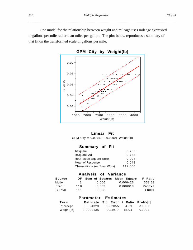
One model for the relationship between weight and mileage uses mileage expressed

in gallons per mile rather than miles per gallon. The plot below reproduces a summary of

that fit on the transformed scale of gallons per mile.

GPM City by Weight(lb)

GP

M C

ity

0 .03

0.04

0.05

0.06

0.07

1500 2000 2500 3000 3500 4000Weight(lb)

Linear FitGPM City = 0.00943 + 0.00001 Weight(lb)

Summary of FitRSquare 0.765RSquare Adj 0.763Root Mean Square Error 0.004Mean of Response 0.048Observations (or Sum Wgts) 112.000

Analysis of VarianceSource DF Sum of Squares Mean Square F RatioModel 1 0.006 0.006426 358.62Error 110 0.002 0.000018 Prob>FC Total 111 0.008 <.0001

Parameter EstimatesT e r m Est imate Std Error t Ratio Prob>| t |Intercept 0.0094323 0.002055 4.59 <.0001Weight(lb) 0.0000136 7.19e-7 18.94 <.0001

110 Multiple Regression Class 4

The units of gallons per mile produce a very small slope estimate since each added

pound of weight causes only a very small increase in fuel consumption per mile. We can

obtain a “friendlier” set of results by rescaling the response as gallons per 1000 miles.

The results follow. Little has changed, but the slope and intercept are 1000 times larger.

The goodness-of-fit measure R2 is the same.

GP1000M City by Weight(lb)GP1

000M C

ity

3 0

4 0

5 0

6 0

7 0

1500 2000 2500 3000 3500 4000Weight(lb)

Linear FitGP1000M City = 9.43234 + 0.01362 Weight(lb)

Summary of FitRSquare 0.765Root Mean Square Error 4.233Mean of Response 47.595Observations (or Sum Wgts) 112

Analysis of VarianceSource DF Sum of Squares Mean Square F RatioModel 1 6426.4 6426.44 358.6195Error 110 1971.2 17.92 Prob>FC Total 111 8397.6 <.0001

Parameter EstimatesT e r m Est imate Std Error t Ratio Prob>| t |Intercept 9.4323 2.0545 4.59 <.0001Weight(lb) 0.0136 0.0007 18.94 <.0001


Before we turn to the task of prediction, we need to check the usual diagnostics.

The residuals in the previous plot do not appear symmetrically distributed about the line.

Notice that several high-performance vehicles have much higher than predicted fuel

consumption.

Saving the residuals lets us view them more carefully. The skewness stands out in

the following normal quantile plot. How does this apparent skewness affect predictions

and prediction intervals from the model?

Residual GP1000M City

- 1 0

- 5

0

5

1 0

1 5.01 .05.10 .25 .50 .75 .90.95 .99

- 3 - 2 - 1 0 1 2 3

Normal Quantile


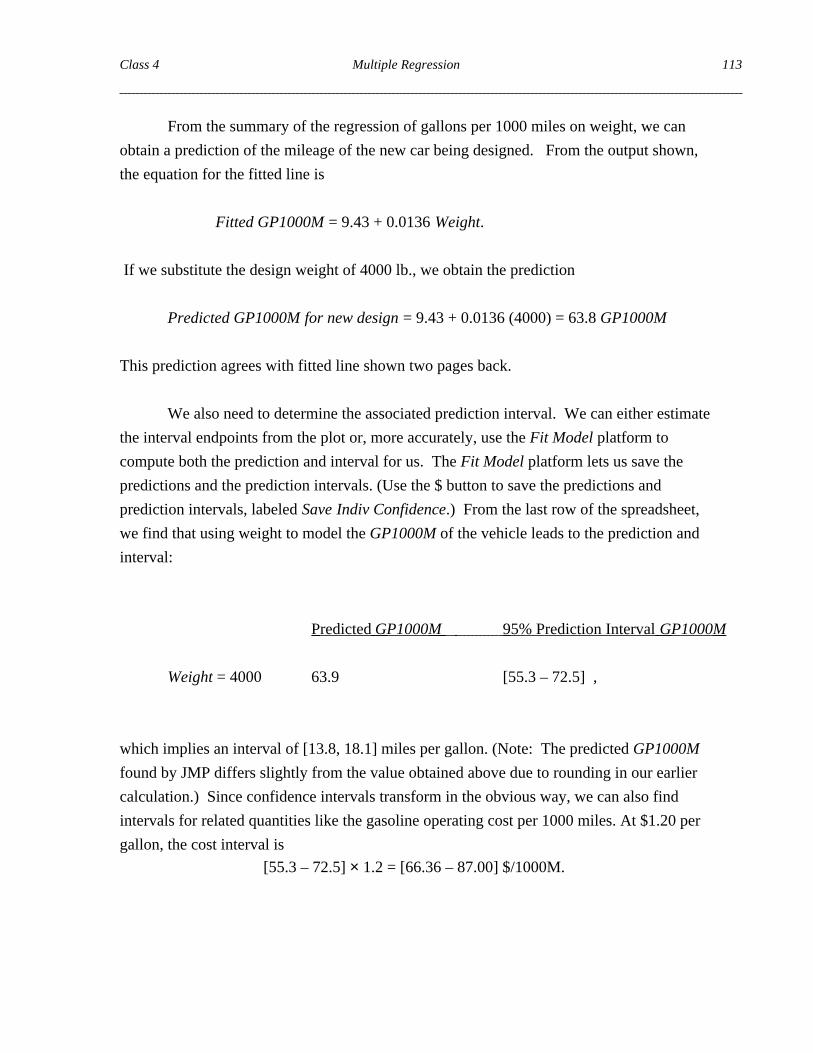
From the summary of the regression of gallons per 1000 miles on weight, we can

obtain a prediction of the mileage of the new car being designed. From the output shown,

the equation for the fitted line is

Fitted GP1000M = 9.43 + 0.0136 Weight.

If we substitute the design weight of 4000 lb., we obtain the prediction

Predicted GP1000M for new design = 9.43 + 0.0136 (4000) = 63.8 GP1000M

This prediction agrees with fitted line shown two pages back.

We also need to determine the associated prediction interval. We can either estimate

the interval endpoints from the plot or, more accurately, use the Fit Model platform to

compute both the prediction and interval for us. The Fit Model platform lets us save the

predictions and the prediction intervals. (Use the $ button to save the predictions and

prediction intervals, labeled Save Indiv Confidence.) From the last row of the spreadsheet,

we find that using weight to model the GP1000M of the vehicle leads to the prediction and

interval:

Predicted GP1000M 95% Prediction Interval GP1000M

Weight = 4000 63.9 [55.3 – 72.5] ,

which implies an interval of [13.8, 18.1] miles per gallon. (Note: The predicted GP1000M

found by JMP differs slightly from the value obtained above due to rounding in our earlier

calculation.) Since confidence intervals transform in the obvious way, we can also find

intervals for related quantities like the gasoline operating cost per 1000 miles. At $1.20 per

gallon, the cost interval is

[55.3 – 72.5] × 1.2 = [66.36 – 87.00] $/1000M.


The search for other factors that are able to improve this prediction (make it more

accurate with a shorter prediction interval) begins by returning to the problem. Weight aside,

what other factors ought to be relevant to mileage? Right away, the power of the engine

(horsepower) comes to mind. Some other factors might be the size of the engine (the engine

displacement is measured in cubic inches; 61 in3 ≈ 1 liter) or the amount of space in the

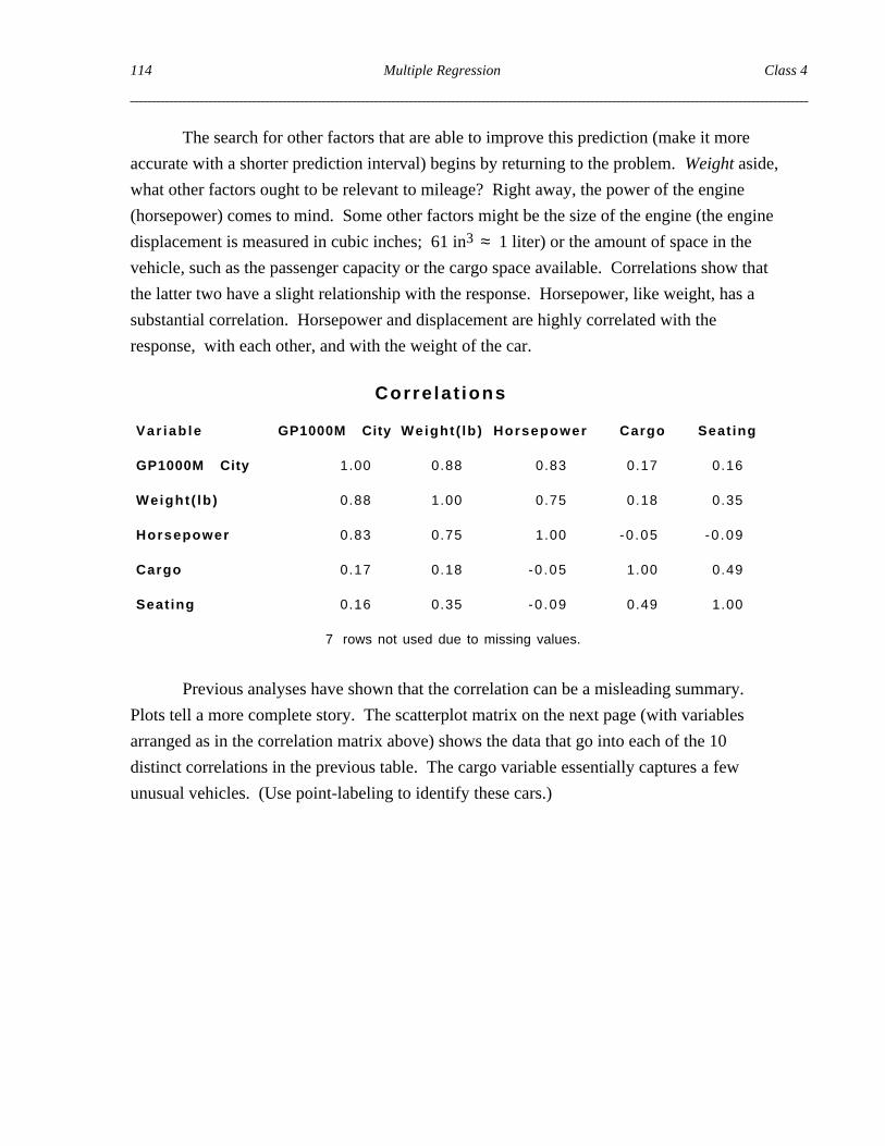
vehicle, such as the passenger capacity or the cargo space available. Correlations show that

the latter two have a slight relationship with the response. Horsepower, like weight, has a

substantial correlation. Horsepower and displacement are highly correlated with the

response, with each other, and with the weight of the car.

Corre la t ions

Var iab le GP1000M City Weight ( lb ) Horsepower Cargo Seat ing

GP1000M City 1.00 0.88 0.83 0.17 0.16

Weight ( lb ) 0.88 1.00 0.75 0.18 0.35

Horsepower 0.83 0.75 1.00 -0 .05 -0 .09

Cargo 0.17 0.18 -0 .05 1.00 0.49

Seat ing 0.16 0.35 -0 .09 0.49 1.00

7 rows not used due to missing values.

Previous analyses have shown that the correlation can be a misleading summary.

Plots tell a more complete story. The scatterplot matrix on the next page (with variables

arranged as in the correlation matrix above) shows the data that go into each of the 10

distinct correlations in the previous table. The cargo variable essentially captures a few

unusual vehicles. (Use point-labeling to identify these cars.)


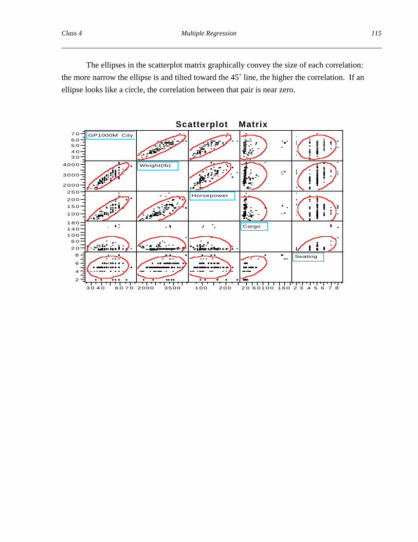
The ellipses in the scatterplot matrix graphically convey the size of each correlation:

the more narrow the ellipse is and tilted toward the 45˚ line, the higher the correlation. If an

ellipse looks like a circle, the correlation between that pair is near zero.

Scatterplot Matrix

3 04 0

5 06 0

7 0

2000

3000

4000

100

150

200

250

2 0

6 0

100

140

180

2

4

6

8

GP1000M City

3 0 4 0 6 0 7 0

Weight(lb)

2000 3500

Horsepower

100 200

Cargo

2 0 6 0100 160

Seating

2 3 4 5 6 7 8


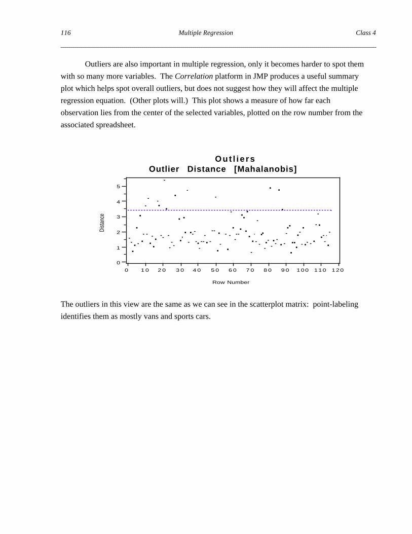
Outliers are also important in multiple regression, only it becomes harder to spot them

with so many more variables. The Correlation platform in JMP produces a useful summary

plot which helps spot overall outliers, but does not suggest how they will affect the multiple

regression equation. (Other plots will.) This plot shows a measure of how far each

observation lies from the center of the selected variables, plotted on the row number from the

associated spreadsheet.

Out l i e r sOutlier Distance [Mahalanobis]

Dist

ance

0

1

2

3

4

5

0 1 0 2 0 3 0 4 0 5 0 6 0 7 0 8 0 9 0 100 110 120

Row Number

The outliers in this view are the same as we can see in the scatterplot matrix: point-labeling

identifies them as mostly vans and sports cars.


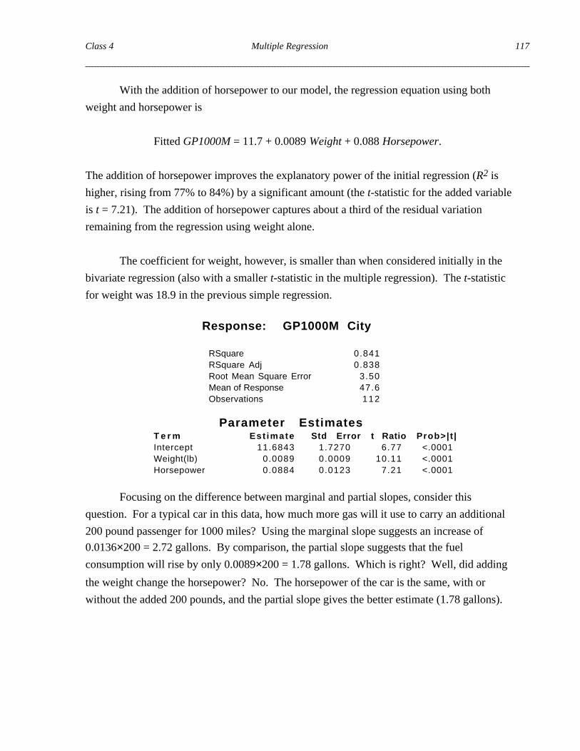
With the addition of horsepower to our model, the regression equation using both

weight and horsepower is

Fitted GP1000M = 11.7 + 0.0089 Weight + 0.088 Horsepower.

The addition of horsepower improves the explanatory power of the initial regression (R2 is

higher, rising from 77% to 84%) by a significant amount (the t-statistic for the added variable

is t = 7.21). The addition of horsepower captures about a third of the residual variation

remaining from the regression using weight alone.

The coefficient for weight, however, is smaller than when considered initially in the

bivariate regression (also with a smaller t-statistic in the multiple regression). The t-statistic

for weight was 18.9 in the previous simple regression.

Response: GP1000M City

RSquare 0.841RSquare Adj 0.838Root Mean Square Error 3.50Mean of Response 47.6Observations 112

Parameter EstimatesT e r m Est imate Std Error t Ratio Prob>| t |Intercept 11.6843 1.7270 6.77 <.0001Weight(lb) 0.0089 0.0009 10.11 <.0001Horsepower 0.0884 0.0123 7.21 <.0001

Focusing on the difference between marginal and partial slopes, consider this

question. For a typical car in this data, how much more gas will it use to carry an additional

200 pound passenger for 1000 miles? Using the marginal slope suggests an increase of

0.0136×200 = 2.72 gallons. By comparison, the partial slope suggests that the fuel

consumption will rise by only 0.0089×200 = 1.78 gallons. Which is right? Well, did adding

the weight change the horsepower? No. The horsepower of the car is the same, with or

without the added 200 pounds, and the partial slope gives the better estimate (1.78 gallons).


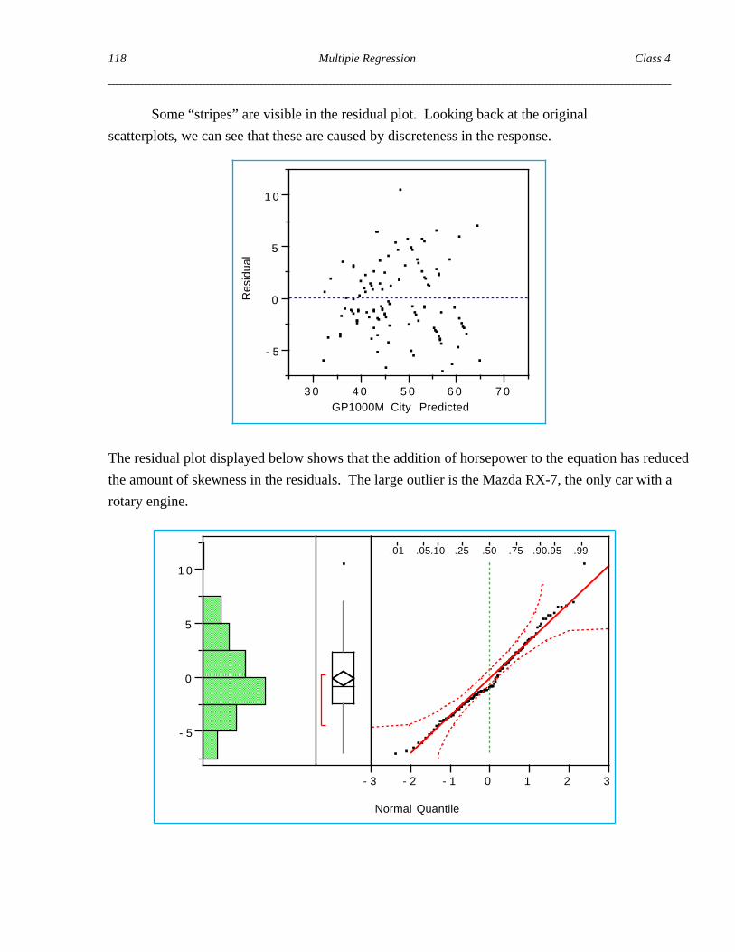
Some “stripes” are visible in the residual plot. Looking back at the original

scatterplots, we can see that these are caused by discreteness in the response.

Res

idua

l

- 5

0

5

1 0

3 0 4 0 5 0 6 0 7 0GP1000M City Predicted

The residual plot displayed below shows that the addition of horsepower to the equation has reduced

the amount of skewness in the residuals. The large outlier is the Mazda RX-7, the only car with a

rotary engine.

- 5

0

5

1 0

.01 .05.10 .25 .50 .75 .90.95 .99

- 3 - 2 - 1 0 1 2 3

Normal Quantile


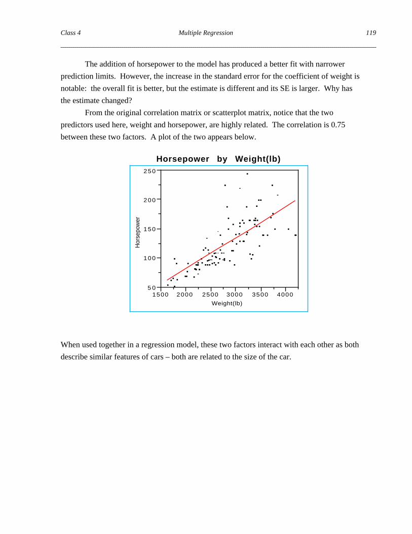
The addition of horsepower to the model has produced a better fit with narrower

prediction limits. However, the increase in the standard error for the coefficient of weight is

notable: the overall fit is better, but the estimate is different and its SE is larger. Why has

the estimate changed?

From the original correlation matrix or scatterplot matrix, notice that the two

predictors used here, weight and horsepower, are highly related. The correlation is 0.75

between these two factors. A plot of the two appears below.

Horsepower by Weight(lb)

Hor

sepo

wer

5 0

100

150

200

250

1500 2000 2500 3000 3500 4000

Weight(lb)

When used together in a regression model, these two factors interact with each other as both

describe similar features of cars – both are related to the size of the car.


Recall that the SE of a slope estimate in a simple regression is determined by three

factors:

(1) error variation around the fitted line (residual variation),

(2) number of observations, and

(3) variation in the predictor.

These same three factors apply in multiple regression, with one important exception. The

third factor is actually

(3) “unique” variation in the predictor.

The effect of the correlation between the two predictors is to reduce the effective range of

weight, as suggested in the plot below. Without Horsepower in the equation, the full

variation of Weight is available for estimating the coefficient for Weight. Restricted to a

specific horsepower rating, much less variation is available. As a result, even though the

model fits better, the SE for Weight has increased.

Hor

sepo

wer

5 0

100

150

200

250

1500 2000 2500 3000 3500 4000

Weight(lb)

Variation in Weight for

HP near 150

Total variation inWeight


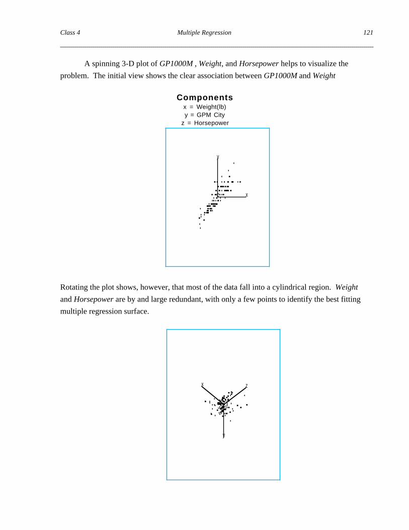
A spinning 3-D plot of GP1000M , Weight, and Horsepower helps to visualize the

problem. The initial view shows the clear association between GP1000M and Weight

Componentsx = Weight(lb)y = GPM City

z = Horsepower

x

y

z

Rotating the plot shows, however, that most of the data fall into a cylindrical region. Weight

and Horsepower are by and large redundant, with only a few points to identify the best fitting

multiple regression surface.

x

y

z


Regression models are more easily interpreted when the predictors are uncorrelated

with each other. We can easily reduce the correlation in this example without losing our

ability to interpret the factors. In particular, based on knowing something about cars,

consider using the power-to-weight ratio, HP/Pound, rather than Horsepower itself.

This new predictor is not so highly correlated with Weight, as shown in the plot that

follows. (The correlation is 0.26.) Typically, whenever companies make a heavier car, they

also increase its horsepower. However, that does not imply that they also increase the

power-to-weight ratio, and so the correlation is smaller.

HP/Pound by Weight(lb)

HP

/Pou

nd

0 .03

0.04

0.05

0.06

0.07

0.08

1500 2000 2500 3000 3500 4000

Weight(lb)

The 3-D spinning plot (not shown) also shows that the data are less concentrated in a cylinder

and have a more planar shape when HP/Pound replaces Horsepower.


Using the power-to-weight ratio in place of horsepower alone yields the following

multiple regression. The goodness-of-fit is comparable to what we obtained using

Horsepower, and the t-statistic for the coefficient of Weight is much higher.


RSquare 0.845RSquare Adj 0.842Root Mean Square Error 3.458Mean of Response 47.595Observations (or Sum Wgts) 112.000

T e r m Est imate Std Error t Ratio Prob>| t |Intercept 0.6703 2.0472 0.33 0.7440Weight(lb) 0.0125 0.0006 20.71 <.0001HP/Pound 270.7381 36.2257 7.47 <.0001

The residuals are similar to those from the prior model, though a bit more normal as you can

check from the residual plot:normality.

- 1 0

- 5

0

5

1 0

.01 .05.10 .25 .50 .75 .90.95 .99

- 3 - 2 - 1 0 1 2 3

Normal Quantile


The next type of residual plot, called a leverage plot in JMP, focuses on a single

multiple regression coefficient. There is one leverage plot for each predictor in the model. A

leverage plot shows the contribution of each variable to the overall multiple regression,

exclusive of the variation explained by others.

• The slope of the line shown in the leverage plot is equal to the coefficient for that

variable in the multiple regression. In this sense, a leverage plot resembles the familiar

scatterplot that makes regression with a single predictor so easy to understand.

• The distances from the points to the line in the leverage plot are the multiple

regression residuals. The distance of a point to the horizontal line is the residual that would

occur if this factor were not in the model. Thus, the data shown in the leverage plot are not

the original variables in the model, but rather the data adjusted to show how the multiple

regression is affected by each factor.

As in simple regression, the slope for a variable is significant if the horizontal line ever lies

outside the indicated confidence bands.


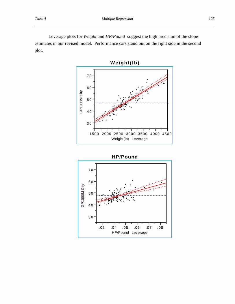
Leverage plots for Weight and HP/Pound suggest the high precision of the slope

estimates in our revised model. Performance cars stand out on the right side in the second

plot.

Weigh t ( lb )

GP

1000

M C

ity

3 0

4 0

5 0

6 0

7 0

1500 2000 2500 3000 3500 4000 4500Weight(lb) Leverage

HP/Pound

GP

1000

M C

ity

3 0

4 0

5 0

6 0

7 0

.03 .04 .05 .06 .07 .08HP/Pound Leverage


Returning to the problem of predicting the mileage of the proposed car, this multiple

regression equation provides narrower prediction intervals than a model using weight alone.

The prediction interval using both variables shifts upward (lower mileage) relative to the

interval from simple regression. The higher than typical power-to-weight ratio of the

anticipated car leads to a slightly higher estimate of gasoline consumption. With more

variation explained, the prediction interval is also more narrow than that from the model with

weight alone.

Model Predicted GP1000M 95% Prediction Interval

Weight alone 63.9 [55.3 – 72.5]

Weight & HP/Weight 64.3 [57.3 – 71.3]

Other factors might also be useful in explaining the cars’ mileage, but the analysis at

this point is guided less by reasonable theory and becomes more exploratory. For example,

adding both cargo and seating indicates that the cargo space affects mileage, even controlling

for weight and horsepower. Seating has little effect (small t-statistic, p-value much larger

than 0.05).

Response: GP1000M CityRSquare 0.854RSquare Adj 0.849Root Mean Square Error 3.39Mean of Response 47.7Observations 109

T e r m Est imate Std Error t Ratio Prob>| t |

Intercept 2.4895 2.8155 0.88 0.3786

Weight(lb) 0.0126 0.0007 17.55 <.0001

HP/Pound 262.0547 44.8848 5.84 <.0001

Cargo 0.0329 0.0132 2.49 0.0142

Seating -0.4875 0.4066 -1 .20 0.2333


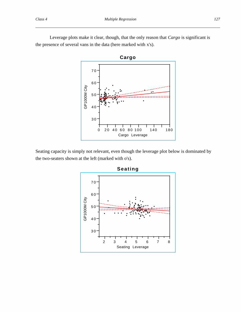
Leverage plots make it clear, though, that the only reason that Cargo is significant is

the presence of several vans in the data (here marked with x's).

Cargo

GP

1000

M C

ity

3 0

4 0

5 0

6 0

7 0

0 2 0 4 0 6 0 8 0 100 140 180Cargo Leverage

Seating capacity is simply not relevant, even though the leverage plot below is dominated by

the two-seaters shown at the left (marked with o's).

Seat ing

GP

1000

M C

ity

3 0

4 0

5 0

6 0

7 0

2 3 4 5 6 7 8Seating Leverage


Further exploration suggests that price is a significant predictor that improves the

regression fit. But why should it be included in the model?

Response: GP1000M CityRSquare 0.866RSquare Adj 0.860Root Mean Square Error 3.26Mean of Response 47.8Observations 107


Intercept 4.1616 2.8146 1.48 0.1424

Weight(lb) 0.0110 0.0010 11.12 <.0001

HP/Pound 255.8825 44.5396 5.75 <.0001

Cargo 0.0334 0.0127 2.64 0.0097

Seating -0.2001 0.4209 -0 .48 0.6355

Price 0.0001 0.0001 2.15 0.0339

Has the addition of these three new predictors significantly improved the fit of our model.

To answer this question, we need to go outside the realm of what JMP provides automatically

and compute the partial F statistic. The idea is to see how much of the residual remaining

after Weight and HP/Pound has been explained by the other three.

F = Change in R2 per added term Remaining variation per d.f. =

(0.866–0.845)/3 (1–0.866)/(107-6) = 5.28 .

Each added coefficient explains about five times the variation remaining in each residual

“degree of freedom”. This is significant, as you can check from JMP’s calculator.


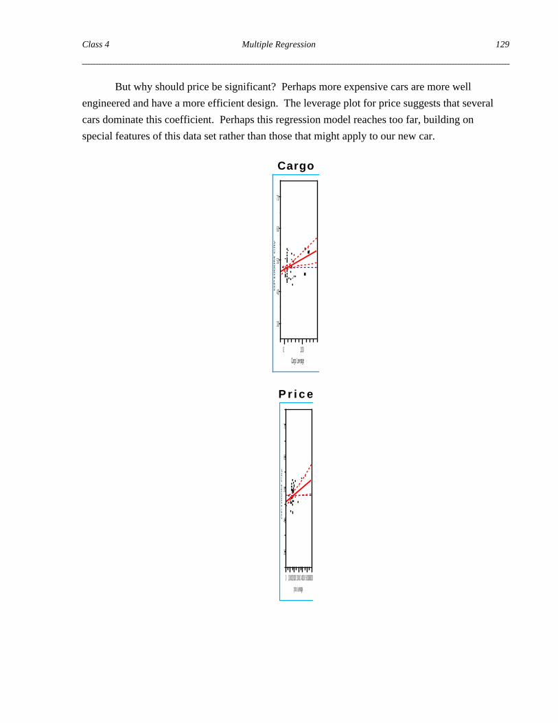
But why should price be significant? Perhaps more expensive cars are more well

engineered and have a more efficient design. The leverage plot for price suggests that several

cars dominate this coefficient. Perhaps this regression model reaches too far, building on

special features of this data set rather than those that might apply to our new car.

Cargo

GP

10

00

M C

ity

3 0

4 0

5 0

6 0

7 0

0 100Cargo Leverage

P r i c e

GP

10

00

M C

ity

3 0

4 0

5 0

6 0

7 0

0 1000020000 30000 40000 5000060000price Leverage


From looking at the leverage plot, it seems that just a small subset of the vehicles

affects these new coefficients. Indeed, if we set aside the four vans and the three expensive

cars on the right of the leverage plot for Price (BMW-735i, Cadillac Allante, Mercedes S),

the regression coefficients for both Cargo and Price are no longer significant. The size of

these changes to the fit suggests that the significant effects for these two factors are perhaps

overstated, relying too much on a small subset of the available data.


RSquare 0.856RSquare Adj 0.848Root Mean Square Error 3.205Mean of Response 47.1Observations 100


Intercept 3.7488 2.9737 1.26 0.2105

Weight(lb) 0.0115 0.0010 11.16 <.0001

HP/Pound 254.2858 46.7636 5.44 <.0001

Cargo 0.0265 0.0262 1.01 0.3147

Seating -0.1904 0.4381 -0 .43 0.6649

Price 0.0000 0.0001 0.62 0.5393


Here are the leverage plots for Cargo and Price, with the seven outlying or leveraged

points excluded. Neither slope estimate differs significantly from zero based on the reduced

data set.

Cargo

GP

10

00

M C

ity

2 5

3 0

3 5

4 0

4 5

5 0

5 5

6 0

6 5

0 2 0 4 0 6 0 8 0 100 120 140 160Cargo Leverage

P r i c e

GP

10

00

M C

ity

2 5

3 0

3 5

4 0

4 5

5 0

5 5

6 0

6 5

0 5000 15000 25000 35000 45000price Leverage


The design team has a good idea of the characteristics of the car, right down to the type of leather

to be used for the seats. However, the team does not know how these characteristics will affect

the mileage.

The goal of this analysis is twofold. First, we need to learn which characteristics of the design

are likely to affect mileage. The engineers want an equation. Second, given the current design,

we need to predict the associated mileage.

The analysis is done on a scale of gallons per 1000 miles rather than miles per gallon.

(1) As expected, both weight and horsepower are important factors that affect vehicle mileage.

Adding the power-to-weight ratio to a simple regression equation leads to a better fit and

more accurate (as well as shifted) predictions.

The inclusion of other factors that are less interpretable, however, ought to be treated

with some skepticism and examined carefully. Often such factors appear significant in a

regression because of narrow features of the data being used to fit the model; such features

are not likely to generalize to new data and their use in prediction is to be avoided.

(2) Using the equation with just weight and the power-to-weight ratio, we predict the mileage of

the car to be in the range

[57.3 – 71.3] GP1000M ⇒ [14.0 – 17.5] MPG

Notice how prediction intervals (like confidence intervals) easily handle transformation —

just transform the endpoints.


regression casebook, 2nd pr - wharton statistics …stine/stat102/autodesign.pdf · from the...

Documents