regression analysis of variates observed on (0, 1 ...bdm25/statmodelling.pdfregression analysis of...

$: Regression analysis of variates observed on (0, 1 ...bdm25/statmodelling.pdfRegression analysis of variates observed on (0, 1): percentages, proportions and fractions Robert Kieschnick1and$
Regression analysis of variates observed on (0, 1):percentages, proportions and fractions

Robert Kieschnick1 and BD McCullough2

1Department of Finance and Managerial Economics, University of Texas at Dallas,Richardson, Texas, USA2Department of Decision Sciences, Drexel University, Philadelphia, PA, USA

Abstract: Many types of studies examine the in�uence of selected variables on the conditional expectationof a proportion or vector of proportions, for example, market shares, rock composition, and so on. Weidentify four distributional categories into which such data can be put, and focus on regression models forthe �rst category, for proportions observed on the open interval (0, 1). For these data, we identify differentspeci�cations used in prior research and compare these speci�cations using two common samples andspeci�cations of the regressors. Based upon our analysis, we recommend that researchers use either aparametric regression model based upon the beta distribution or a quasi-likelihood regression modeldeveloped by Papke and Wooldridge (1997) for these data. Concerning the choice between these tworegression models, we recommend that researchers use the parametric regression model unless their samplesize is large enough to justify the asymptotic arguments underlying the quasi-likelihood approach.

Key words: fractions; percentages; proportions; regression

Data and software link available from: http://stat.uibk.ac.at/SMIJReceived July 2002; revised October 2002; accepted March 2003

1 Introduction

Many studies in different disciplines examine how different variables in�uence somepercentage, or proportion, or fraction or vector of such variates. For example, Webb(1983) studies the determinants of cable television subscribership as measured by theproportion of houses that are passed by a cable system that subscribe to that system. Asanother example, DeSarbo et al. (1993) study the proportions of household televisionviewing across different streams of programming.

We surveyed many such studies and arrived at two broad conclusions. Our �rstbroad conclusion is that the data being analysed can be put into one of fourdistributiona l categories. The �rst distributiona l category comprises proportions onthe open interval (0, 1). Figure 1 illustra tes such data using cable penetration data (theproportion of homes that have cable in each of 278 different market areas). The seconddistributiona l category comprises proportions observed on the closed interval [0, 1].

Address for correspondence: R Kieschnick, University of Texas at Dallas, PO Box 830688, JO5.1Richardson, Texas 75083-0688, USA. E-mail: [email protected]

Statistical Modelling 2003; 3: 193–213

# Arnold 2003 10.1191=1471082X03st053oa

Figure 2 illustra tes such data using US corporate capital structure data. A comparisonof Figures 1 and 2 reveals a critical difference between these two types of data:observations at 0 or 1 are typically mass points. (Most software procedures forproducting histograms do not automatically capture point masses. The leftmost bin

Figure 1 Distribution of cable penetration with superimposed normal distribution

Figure 2 Distribution of corporate debt loads with superimposed normal distribution (crosshatched binrepresents the mass point at zero)

194 R Kieschnick and BD McCullough

in this histogram represents 454 observations with the value zero. The number of binsfor all histograms was determined using the method of Scott (1979).) Consequently,while the data in the �rst distributiona l category can be modeled using a continuousdistribution, the data in the second distributiona l category cannot, because they followa mixed discrete–continuous distribution.

Our third and fourth distributional categories are multivariate extensions of the �rsttwo distributional categories. For example, one might be interested in the proportion ofa household’s wealth invested in different classes of assets. If the investment classes arebroad enough, then typically each household has some of its wealth invested in each ofthe categories and there are no boundary observations. Thus, our third distributiona lcategory comprises vectors of proportions for which no component proportion is aboundary observation (e.g., 0s or 1s). However, if the investment classes are morenarrowly de�ned, then a number of households will not have some of their wealth insome of these classes. Consequently, our fourth distributiona l category comprisesvectors of proportions in which some component proportions are boundary observa-tions. Each of these distributiona l categories presents additional problems that do notoccur in their univariate analogs, such as the structure of the correlations betweenelements of these vectors.

The second broad conclusion that we derive from our survey of the publishedliterature is that there are no commonly accepted distributiona l models for these data,nor any commonly accepted regression models for these data. Further, some of theregression models for these data appear dubious at best. For example, we �nd thatresearchers most frequently estimate the parameters of a linear regression model for the�rst two distributiona l categories using ordinary least squares (OLSs). However, such anapproach contravenes two conditions: the conditional expectation function must benonlinear since it maps onto a bounded interval; and its variance must be heteroskedasticsince the variance will approach zero as the mean approaches either boundary point.

The diversity of practices and the questionable nature of some of these practicesmotivate this study. We, however, only focus on our �rst distributional category,proportions observed on (0, 1), because the issues presented by our other three categoriesare quite different, and yet might build in some degree upon how one addresses this �rstcategory. For this category, we surveyed the literature to identify the various speci�ca-tions employed in prior research and synthesized the various practices into a number ofgroups. We present the essentials of these groups in section 2.

In section 3, we use a common data set, cable penetration data, and a common set ofregressors to compare the different regression models. We do this, rather than performa Monte Carlo based comparison, because a Monte Carlo study would have requiredus to assume some data generating process. However, there is no clear agreement on thedata generating process for such data. Thus, we �t the different regression models to acommon data set using a common speci�cation of the regressors to determine whichregression model best describes the data.

In section 4, we repeat the analysis reported in section 3, but this time using adifferent data set, voting for President Bush in the 2000 Presidential election. We do thisto check the robustness of our conclusions about which regression model best describesthis distributiona l category of proportional data.

Regression analysis of variates observed on (0, 1) 195

Section 5 concludes our paper by providing a summary of our �ndings and directionsfor further research. Our basic recommendation is that researchers use either the betaregression model developed herein or a quasi-likelihood model developed in Papke andWooldridge (1996). Our case studies suggest that the larger the sample, the closer theresults of these models will be, but that in small samples the beta regression model ispreferred.

2 Alternative regression models

We searched the literature to identify how different researchers conducted regressionanalyses of proportions observed on (0, 1), and what their regression models impliedabout their maintained assumptions. (Speci�cally, we searched various electronicdatabases for the keywords percentage, proportion and fraction, to identify potentiallyrelevant research.)

While there are a variety of ways that we could organize the different approaches weobserved in published papers, we use the likelihood principle to organize our discus-sion. From the likelihood principle viewpoint, such research assumes that h(x, y)implies f (yjx)g(x) and E(yjx) ˆ k(x), where k(¢) is a function of a vector of exogenousvariables and h(x, y) is the joint distribution of x and y. (Sometimes k(x) is called theresponse function, and sometimes it is called the conditional expectation function.)Thus we will distinguish approaches according to what the researcher assumed aboutk(x) and f (yjx). Further, we will distinguish between parametric and quasi-parametricspeci�cations of f (yjx).

2.1 Parametric regression models

We organize our discussion of the identi�ed parametric regression models in order oftheir frequency of use. In this regard, we should note that the �rst three regressionmodels account for most of what we observe being used in published papers. The lastthree regression models are rarely used. Because the normal distribution �guresprominently in the commonly used models, all our histograms have superimposed anormal distribution parameterized by the sample mean and sample variance.

2.1.1 Normal distribution: linear response function

By far the most common practice of researchers is to apply OLS to their data (Mehran,1995). The use of OLS presents a problem in characterizing these studies, as sometimesthe sample sizes were large enough to invoke asymptotic arguments to rationalize lessstringent characterizations of their regression models. Nevertheless, we focus on theirmost stringent characterization, for as Godfrey (1988) points out, when these research-ers examine t tests or F tests, they are implicitly assuming that the conditionaldistribution is a normal distribution unless the sample size is large. Further, somecommonly reported tests (e.g., Breusch–Pagan’s test for heteroskedasticity) assume thatthe conditional distribution is a normal distribution regardless of sample size.


Consequently, we categorize all such studies as implicitly assuming a conditionalnormal distribution for their regression model (i.e., f (yjx) is N(k(x), s2 )). In additionto assuming a conditional normal distribution, these researchers also assume that k(x) isequal to x0b, that is, that the conditional expectation function is linear.

Conceptually this approach is subject to a number of �aws. First, it is obvious thatproportions are not normally distributed because they are not de�ned over <, which isthe domain over which the normal distribution is de�ned. A quick examination of anyof our �gures con�rms this point. Further, as mentioned earlier, the fact that thesevariables are only observed over a closed interval implies that the conditional expecta-tion function must be nonlinear, and that the conditional variance must be a function ofthe mean. Clearly, both of these conditions are violated by the assumptions of thisregression model.

2.1.2 Additive logistic normal distribution

The next most frequent practice we observed is that the researcher would transform thedependent variable and then �t a linear response function to the transformed dependentvariable using the least squares principle (Demsetz and Lehn, 1985). While it is notalways clear what the researcher is assuming about the conditional distribution of theuntransformed variable, it was possible to infer their assumptions in all the studies weexamined, because they all used the logit transformation. (Atkinson (1985) devotes achapter to discussing various transformations for percentages and proportions. Whilewe cannot report �nding any studies that follow Atkinson’s proposed approach forimplementing these transformations, we do note that most of the transformations hestudied have the logit transformation as a limiting case.)

The logit regression model has a long history in economics and related disciplines (seeDyke and Patterson (1952) for its earliest development). Using this approach, research-ers (e.g., Webb, 1983) will estimate:

lny

1 ¡ y

³ ´ˆ x0b ‡ E (2:1)

where ln(y=(1 ¡ y)) is the logit transform of the dependent variable using the leastsquares principle. Thus, as noted earlier, these researchers are assuming that E isdistributed N(0, s).

Aitchison (1986) calls the above transformation the additive logratio transformation,and shows that z ˆ ln(y=(1 ¡ y)) will follow a normal distribution, N(m, s2), if y followsan additive logistic normal distribution. Thus, if y is distributed according to anadditive logistic normal distribution, then E is distributed according to the standardnormal distribution. (Aitchison (1986) proposes that one should test if y is distributedas an additive logistic normal distribution by testing if z is normally distributed. Wefollow his proposed testing strategy in our subsequent analysis by testing if E isdistributed as a standard normal random variate.)

The obvious concern with the application of this regression model to the analysis ofproportions is that it assumes, �rst, that the link function (using generalized linear


model terminology) is the logit function, and second, that this transformation stabilizesthe conditional variance. The �rst concern is lessened by evidence reported in Cox(1996) on different link functions for these data. The second concern, however, remainsimportant since alternative distributiona l models for these data (e.g., the beta andsimplex distributions) imply that such a transformation will not stabilize the variance.

2.1.3 Censored normal distribution

Recently, researchers have begun to apply the censored normal model, or Tobit model,to proportional data (e.g., Barclay and Smith, 1995). Speci�cally, such researcherstypically assume that:

y¤i ˆ x0

ib ‡ ui, i ˆ 1, 2, . . . , n (2:2)

and

yi ˆ0, y¤

i µ 0y¤

i , 0 < y¤i < 1

1, y¤i ¶ 1

8<

: (2:3)

where {ui} are assumed to be i.i.d. draws from a N(0, s2 ) distribution.There are problems with the use of this approach to examining the conditional

expectation of a proportion observed over the interval (0, 1). First, one is making theassumption that y¤

i is normally distributed, but only observes values within a speci�edrange. We fail to observe values outside the [0, 1] range for proportional data notbecause they are censored, but because they are not de�ned outside this interval. Thus,there is no censoring, and the censored normal model is inappropriate for these data(see Maddala (1991) for further discussion of this point). Second, for the data observedon the interval (0, 1), the Tobit regression is observationally equivalent to the normalregression model. Thus the Tobit regression model is subject to the same criticisms asthe linear normal regression model.

2.1.4 Normal distribution: nonlinear response function

Another alternative is to �t a nonlinear regression model to these data using leastsquares. For example, Hermalin and Wallace (1994) use the cumulative normalfunction as their conditional expectation function and estimate its parameters usingleast squares.

Rather than follow their practice, we will model the conditional expectation functionin our study using the cumulative logistic function because of the evidence reported inCox (1996) and because it will allow us to focus more on the effect of distributiona lassumptions. Further, this speci�cation is consistent with the speci�cation recom-mended in Kmenta (1986) for these data. Speci�cally, we assume:

yi ˆ 11 ‡ e¡(a‡bx i)

‡ Ei (2:4)


where Ei follows N(0, s2) distribution. We will estimate this equation using the leastsquares principle, as that comports with prior practice.

2.1.5 Beta distribution

Johnson et al. (1995) provide over a dozen examples from different physical sciences inwhich the beta distribution was found to be a better �tting distribution for theproportional data under study than considered alternatives. Hviid and Villadsen(1995) provide a recent example from economics. Even textbooks have suggested thatthe beta distribution is a good distributiona l model for proportional data. For example,Mittelhammer (1996, pp. 195–97) uses an example of the proportion of a tankcontaining heating oil measured at different times to illustra te the beta distribution.

All of these examples assume that y is distributed as follows:

f (y) ˆ 1B(p, q)

yp¡1 (1 ¡ y)q¡1 (2:5)

where 0 µ y µ 1 and B(p, q) is the beta function. We will focus on this two-parameterbeta distribution, rather than the generalized beta distribution developed in McDonaldand Xu (1995), for two reasons. First, it is the distribution most often �tted toproportional data in prior literature and so it is the distributiona l assumption thathas the most empirical support. Second, this family of distributions is part of the class ofexponential distributions, which have served as the basis for the generalized linearmodel paradigm. (see Mittelhammer (1996, pp. 213–15) for a discussion of theexponential class of distributions, and see McCullagh and Nelder (1989) for adiscussion of the generalized linear model paradigm.)

One approach to specifying a beta regression model is to follow the linear regressionmodel and assume that the mean is a linear function of the exogeneous variables. This isthe approach taken in the econometrics program SHAZAM version 7 (Vancouver,Canada) and is also the approach taken in McDonald and Xu (1995). Speci�cally,SHAZAM’s user manual sets out the following model. They assume that y is distributedas a beta random variate and that

E(yjx) ˆ pp ‡ q

ˆ x0b (2:6)

Further they assume that q is the parameter that is conditional on x and so they derive:

q(x) ˆ px0b

¡ p (2:7)

They substitute (2.7) into (2.5) above to derive the conditional density function (i.e.,f (yjx)). They then derive the log-likelihood function for the beta regression model usingthis speci�cation.

This approach does not, however, restrict the range of the conditional mean. Thus itimplicitly requires restrictions on the values of the exogeneous variables to give sensibleresults. Such restrictions are not recognized in SHAZAM’s estimation of this model,


and so the beta regression model speci�ed in SHAZAM is not a very good approach tospecifying a beta regression model.

We argue that a better approach is derived by considering the work of Cox (1996),who tested various link functions for regression models of continous proportions usingthe quasi-likelihood framework. Based upon Cox’s evidence, we use the logit linkspeci�cation. (Separate from Cox’s evidence, we are also motivated to use the logit linkspeci�cation so that there is a consistency in our �rst moment speci�cation acrossdifferent parametric and quasi-parametric models.) Speci�cally, we assume that

E(yijxi) ˆ mi ˆ h(Zi) ˆ 11 ‡ exp(¡Zi)

ˆ 11 ‡ exp(¡x0

ib)(2:8)

This equation then implies the following re-expression:

Zi ˆ g(mi) ˆ lnmi

1 ¡ mi

³ ´ˆ x0

ib (2:9)

Note that this speci�cation restricts the conditional mean of a beta distributedregressand to the interval (0, 1), which is appropriate for this distributiona l model.

In order to derive an estimatable regression model, we must now relate the aboverelationships to the parameters of the beta distribution. Speci�cally, for the betadistribution de�ned in (2.5), we have

E(yi) ˆ pp ‡ q

(2:10)

We map x0ib into q because q is the shape parameter for the beta distribution. Given this

approach, we develop the following expression for q that is consistent with equation(2.10) above:

q(xi) ˆ p exp(¡x0ib) (2:11)

We then substitute this expression for q into (2.5) to derive the conditional distributionof the beta distributed random variate:

f (yijxi) ˆ G(p)G(q(xi))G(p ‡ q(xi))

µ ¶¡1

yp¡1i (1 ¡ yi)

q(xi)¡1

ˆ G(p ‡ q(xi))G(p)G(q(xi))

µ ¶yp¡1

i (1 ¡ yi)q(xi)¡1 (2:12)

To estimate the effect of the different conditioning variables (x1 , x2 , . . . , xr) we can usethe maximum likelihood estimation principle to derive estimates of the vector b bymaximizing the implied log-likelihood function with respect to the parameters b and p .


Because the beta distribution is a member of the exponential class of distributions, thesemaximum likelihood estimators have all the statistical properties established formaximum likelihood estimators for this class of distributions (see Jorgensen (1983)or Fahrmeir and Tutz (1994) for further discussion of these issues and the literatureaddressing them).

2.1.6 Simplex distribution

Our �nal parametric regression model for proportions measured on (0, 1) is based uponthe simplex distribution developed by Barndorff-Nielsen and Jorgensen (1991) for suchdata. Jorgensen (1997) argues that this distribution has the virtue of being a dispersionmodel, while the beta distribution is not. Consequently the analysis of devianceapproach to generalized linear models can be applied to regression models basedupon the simplex distribution, and not to regression models based upon the betadistribution.

We follow Jorgensen (1997) and de�ne the univariate simplex distribution as:

f (y; m, s2 ) ˆ [2ps2 {y(1 ¡ y)}3 ]¡1=2 exp ¡12d(y; m)

© ª(2:13)

for 0 < y < 1, where

d(y; m) ˆ (y ¡ m)2

y(1 ¡ y)m2(1 ¡ m)2 (2:14)

is the unit deviance, and 0 < m < 1. We can either maximize the associated log-likelihood function or minimize the associated unit deviance function to estimate aregression model based upon this distribution. Again, following the evidence of Cox(1996) and our speci�cation of the beta regression model, we assume that the linkfunction, g(m), is the logit link function.

2.2 Quasi-parametric regression models

The prior approaches have presumed some speci�c family of distributions for theconditional distribution for the proportions under study. Cox (1996) and Papke andWooldridge (1996) take a different tack and use the quasi-likelihood approach. Thequasi-likelihood approach speci�es the �rst and second moments of the conditionaldistribution, but does not specify the full distribution.

Cox (1996) examines the �t of four speci�cations of the �rst two moments of theconditional distribution to two samples of proportional data observed over the interval(0, 1). Speci�cally, he examines the use of the logit and complementary log-log linkfunctions, with canonical and orthogonal speci�cations for the variance functions. Heconcludes that the logit link function with the orthogonal variance function is thepreferred combination for his data sets. (Cox describes his use of the terms canonicaland orthogonal speci�cations and speci�es on p. 455 his examined combinations.


His preferred combination, which he calls the orthogonal pair, is: m(y) ˆ 1=(1 ‡ e¡y);u(m) ˆ m2(1 ¡ m)2 .)

Papke and Wooldridge (1996) use a similar approach, but for a slightly differentproblem. They are interested in specifying a quasi-likelihood regression model forcontinuously measured proportions with a �nite number of boundary observations (i.e.,0s and 1s). They use the following log-likelihood speci�cation,

`i(b) ˆ yi ln[G(xi)] ‡ (1 ¡ yi)ln[1 ¡ G(xi)] (2:15)

which they point out is well de�ned for 0 < G(¢) < 1. While Papke and Wooldridgediscuss the use of different speci�cations for G(¢), they use the logistic function in theiranalysis, which is equivalent to Cox’s logit link speci�cation. Further, they use a slightlymore robust approach to the estimation of the standard errors. Consequently we willfocus on their approach in the subsequent analysis.

2.3 Comparing regression models

We have presented the essentials of various regression approaches that have beenapplied to the analysis of proportions observed on the interval (0, 1). While we havegiven reasons to question the application of one or another of these approaches to thiskind of data, we now turn to a comparison of their application to real data to judgetheir relative merits. We do this because, as stated earlier, there is no agreement in theliterature on the proper probability models for these data.

3 Case study 1: cable penetration

3.1 Description of the data

We �rst examine in�uences on cable penetration. To do this we will use a sample thatwas collected by the Federal Communications Commission (FCC) in conjunction withthe implementation of the Cable Television Consumer Protection and Competition Actof 1992. On 23 December 1992 the FCC mailed out 748 questionaires to a strati�edsample of ‘cable community units,’ which are essentially individual franchise areas. Ofthe 748 questionaires sent out, 687 respondents supplied usable responses on prices,costs and other cable operator data for each franchise. Because the sampling metho-dology and data elements requested in the questionaire are described in detail inAppendix E of FCC 93-177, we will refer the reader to this source for further discussionof these topics (Federal Communications Commission, 1993).

To supplement these data, the FCC collected additional economic and demographicinformation from the US Department of Commerce, Census Bureau. Appendix C ofFCC 94-38 describes the data, matching procedures (i.e., county to cable communityunit matching), and variable de�nitions used to extend the original sample data foradditional economic and demographic information (Federal Communications


Commission, 1994). Again, we refer the reader to this source for detailed descriptionsof the added data.

For the above sample, we will only use a portion of the data collected as we are moreinterested in comparing the results of different regression procedures than in exploringthe best speci�cation of regressors. Consequently we use the same set of regressors ineach estimated regression model to focus on the effect of the statistical model on theresults obtained. Speci�cally, we use:

E(yjx) ˆ h(b0 ‡ b1 lin ‡ b2child ‡ b3ltv ‡ b4dism ‡ b5agehe) (3:1)

In this equation, we are using the logarithm of franchise median income (lin), thepercentage of franchise households with children (child), the number of local broadcasttelevision signals (ltv), the age of the cable system headend (agehe), and a measure ofconsumer dissatisfaction with the cable operator (dism). The dependent variable,displayed in Figure 1, is the proportion of households within a market area thatsubscribe to cable television.

We include the logarithm of franchise median income because prior studies (e.g.,Park, 1972; Reagan et al., 1985, etc.) have shown household income to in�uence ahousehold’s decision to subscribe to cable television. We adjust for scale effects by usingthe logarithm of median franchise income. We include the percentage of franchisehouseholds with children because prior studies (e.g., Park, 1972; Reagan et al., 1985)have shown that the presence of children in a household is a signi�cant in�uence on ahousehold’s decision to subscribe to cable television. We include the number of localbroadcast television signals because prior studies (e.g., Park, 1972) have found thenumber of local broadcast television signals available to a household to be a signi�cantlynegative in�uence on whether a household subscribes to cable television. We include theage of the cable system headend because this proxies for extent of diffusion of the cablesystem within its franchise (see Sparkes and Kang (1986) for further discussion of whythis is important). Finally we create a consumer satisfaction variable, dism, bycomputing the number of net disconnectors (number of disconnecting households 7number of reconnecting households) and substracting this number from the number ofnew subscribing households. We presume that if more households are leaving a cablesystem than entering it, then consumers are dissatis�ed with the service provided by thecable system operator. LaRose and Atkin (1988), Atkin (1992), and Albarran andUmphrey (1994) provide evidence that such a variable signi�cantly in�uences cablepenetration.

3.2 Comparison of regression models

In Table 1, we report the results of �tting the various regression models described aboveto the data, also described above. Before discussing these results, we should address acouple of computational issues since a number of these regression models requirenonlinear optimization to derive parameter estimates. First, starting values for thecoef�cients of the independent variables were obtained from the logit or logistic normalregression model as its conditional expectation is consistent with the functional form oftheir conditional expectation function. (We estimated the simplex regression model by


Tab

le1

Res

ult

sfo

rd

iffe

ren

tre

gre

ssio

nm

od

els

of

cab

lep

enet

rati

on

k…x

†f…y

jx†

Lin

ear

no

rmal

Lin

ear

cen

sore

dn

orm

alT

ran

sfo

rmed

log

isti

cn

orm

alLo

gis

tic

no

rmal

Log

isti

cb

eta

Logi

stic

sim

ple

xLo

gis

ticu

nsp

eci�

ed

Est

imat

ion

met

ho

da

LSM

LLS

LSM

LM

LQ

ML

con

stan

tb¡

0.14

53¡

0.14

53¡

3.06

96*

¡2.

7391

**¡

1.92

21*

¡2.

5985

*¡

2.85

47**

(0.2

815)

(0.2

784)

(1.5

643)

(1.2

177)

(1.1

283)

(1.4

054)

(1.2

911)

lin0.

0763

**0.

0763

**0.

3679

**0.

3215

**0.

2424

**0.

3497

**0.

3340

**(0

.028

8)(0

.028

5)(0

.160

0)(0

.124

8)(0

.111

3)(0

.148

4)(0

.131

8)ch

ild0.

0007

0.00

070.

0027

0.00

290.

0031

¡0.

0017

0.00

29(0

.001

0)(0

.009

7)(0

.005

4)(0

.004

2)(0

.004

6)(0

.006

5)(0

.004

1)lt

v¡

0.01

47**

¡0.

0147

**¡

0.07

7**

¡0.

0622

**¡

0.05

92**

¡0.

0795

**¡

0.06

42**

(0.0

033)

(0.0

033)

(0.0

184)

(0.0

146)

(0.0

145)

(0.0

174)

(0.0

136)

dis

mc

¡0.

4082

¡0.

4082

¡1.

7529

¡1.

6576

¡1.

9455

**¡

2.14

07**

¡1.

6175

**(0

.298

6)(0

.298

6)(1

.658

9)(1

.245

0)(0

.493

4)(0

.725

0)(0

.555

8)ag

ehe

0.00

62**

0.00

62**

0.03

38**

0.02

82**

0.02

58**

0.02

61**

0.02

83**

(0.0

012)

(0.0

012)

(0.0

067)

(0.0

048)

(0.0

059)

(0.0

071)

(0.0

056)

AIC

cd¡

1.45

25¡

1.45

25¡

2.48

35¡

2.63

34¡

2.73

95¡

2.63

34¡

2.73

77

aLS

,le

ast

squ

ares

;M

L,m

axim

um

likel

iho

od

;QM

L,q

uas

i-m

axim

um

likel

iho

od

.bS

tan

dar

der

rors

are

rep

ort

edin

par

enth

eses

bel

ow

coef

�ci

ent

esti

mat

e.**

Sig

ni�

can

ceat

the

5%le

vel;

*si

gn

i�ca

nce

atth

e10

%le

vel.

c dis

mw

assc

aled

by

1=10

000

0in

ord

erto

pro

du

ceco

ef�

cen

tso

fth

esa

me

mag

nit

ud

eas

the

oth

erco

ef�

cien

ts.

dT

his

stat

istic

rep

rese

nts

ave

rsio

no

fth

eA

kaik

eIn

form

atio

nC

rite

ria

der

ived

inM

cQu

arri

ean

dT

sai

(199

8).


both maximizing its associated log-likelihood function and by minimizing its unitdeviance function. Each approach gave the same results, but the second approachconverged to a solution in 1

6 the number of iterations. Consequently we recommend theuse of the second approach for estimating these types of regression models.) In addition,the beta regression model requires a starting value for p, which we derived by �tting thetwo-parameter beta distribution to our sample data using both maximum likelihoodand method of moment estimators. (For this we use a STATA program developed byNicholas Cox to implement procedures developed in Mielke (1975). Note, however,that the coef�cient estimates of the beta regression model were very robust with respectto variations of our starting parameter estimates. Consequently it is clear that thesestarting values were not important to our �nal estimates.) Second, all functions wereoptimized and standard deviations estimated using �rst and second analytic derivativeswhere appropriate (derivatives were con�rmed using Mathematica (version 4)). Third,we used both STATA (version 7) and TSP (version 4.5) on a Pentium 400 PC runningunder Windows 2000 to perform our computations in order to con�rm that our resultswere robust across software packages. (In an earlier draft, we used S-PLUS v4.5 release2 on a Pentium 400 PC running Windows 98 and obtained similar estimates to thosereported.) Given these computational notes, we begin our discussion of our results.

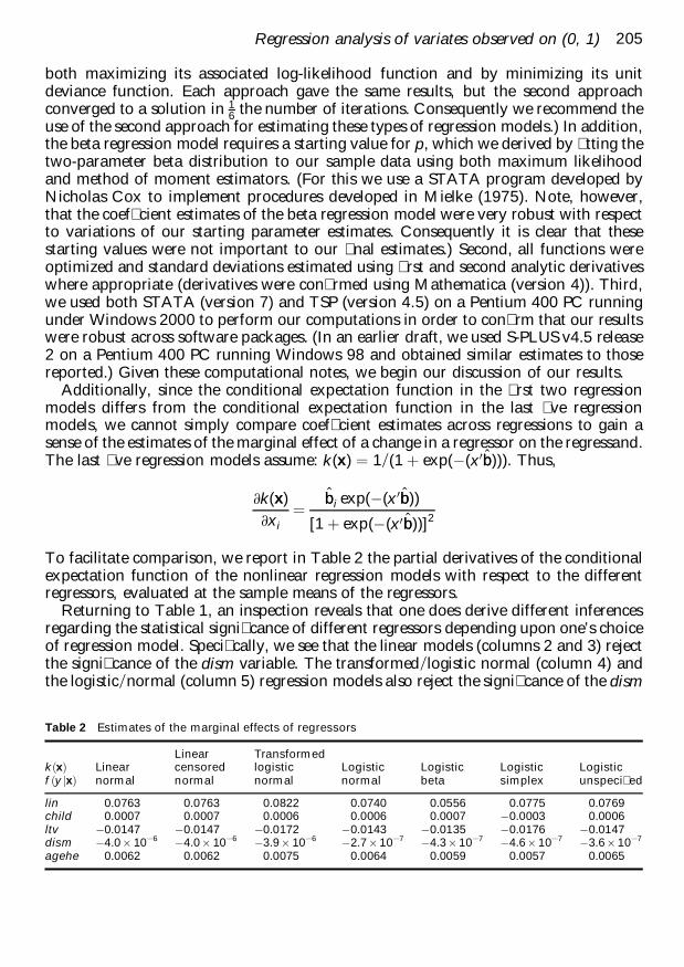
Additionally, since the conditional expectation function in the �rst two regressionmodels differs from the conditional expectation function in the last �ve regressionmodels, we cannot simply compare coef�cient estimates across regressions to gain asense of the estimates of the marginal effect of a change in a regressor on the regressand.The last �ve regression models assume: k(x) ˆ 1=(1 ‡ exp(¡(x0bb))). Thus,

@k(x)@xi

ˆ bbi exp(¡(x 0bb))

[1 ‡ exp(¡(x0bb))]2

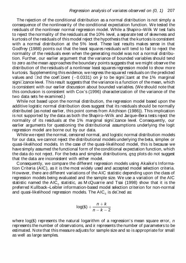
To facilitate comparison, we report in Table 2 the partial derivatives of the conditionalexpectation function of the nonlinear regression models with respect to the differentregressors, evaluated at the sample means of the regressors.

Returning to Table 1, an inspection reveals that one does derive different inferencesregarding the statistica l signi�cance of different regressors depending upon one’s choiceof regression model. Speci�cally, we see that the linear models (columns 2 and 3) rejectthe signi�cance of the dism variable. The transformed=logistic normal (column 4) andthe logistic=normal (column 5) regression models also reject the signi�cance of the dism

Table 2 Estimates of the marginal effects of regressors

k…x†f …y jx†

Linearnormal

Linearcensorednormal

Transformedlogisticnormal

Logisticnormal

Logisticbeta

Logisticsimplex

Logisticunspeci� ed

lin 0.0763 0.0763 0.0822 0.0740 0.0556 0.0775 0.0769child 0.0007 0.0007 0.0006 0.0006 0.0007 ¡0.0003 0.0006ltv ¡0.0147 ¡0.0147 ¡0.0172 ¡0.0143 ¡0.0135 ¡0.0176 ¡0.0147dism ¡4.0 £ 10¡6 ¡4.0 £ 10¡6 ¡3.9 £ 10¡6 ¡2.7 £ 10¡7 ¡4.3 £ 10¡7 ¡4.6 £ 10¡7 ¡3.6 £ 10¡7

agehe 0.0062 0.0062 0.0075 0.0064 0.0059 0.0057 0.0065


variable. In contrast, the beta, simplex and quasi-likelihood models (columns 5, 6 and 7)do not.

In addition to demonstrating that one’s choice of regression model for these datain�uences one’s inferences, these results illustra te two other important points. First, thefact that the beta, simplex and quasi-likelihood model pick up the signi�cance of thedism variable while the other regression models do not, comports with our criticisms ofthe homoskedasticity assumption of these models. Consistent with this conjecture, wenote that for the transformed=logistic normal (column 4) and the logistic=normal(column 5) regression models, the dism variable becomes statistically signi�cant whenwe correct the standard errors for heteroskedasticity. Second, the results of the beta andquasi-likelihood models comport with discrete choice studies of the cable subscriptiondecision. One of the reasons for examining cable penetration data is that we couldrelate our results using aggregate data to results using disaggregate data to discernwhich models for proportional data gave similar results to those of individual choicedata. Several probit analyses have shown that consumer satisfaction with a cable service(our dism variable) is an important determinant of the cable subscription decision.Consequently we conclude that the beta, simplex and quasi-likelihood models providesimilar conclusions to those derived in discrete choice studies.

Inspection of Table 2 suggests that there is not much difference across regressionmodels in their estimates of the marginal effects of the various regressors whenevaluated at the same means of the regressors. This result is not surprising in that thelinear models should be �rst-order approximations to a nonlinear surface whenevaluated at the sample means. Despite this point, we note that the nonlinear modelstend to ascribe a much lower marginal effect to the dism variable than do the linearmodels. Further we must point out the linear and nonlinear models will give quitedifferent estimates of the marginal effects of different regressors as those regressors areevaluated at points other than their means. This fact should not be overlooked whenevaluating the economic signi�cance or policy implications of one’s regression results.

Turning to an analysis of the distributiona l assumptions of the different regressionmodels, we �nd evidence to reject the normal, the censored normal and the logisticnormal distributional assumptions. We �nd that either a Shapiro–Wilk or a Jarque–Bera test rejects the normality of the residuals of the �rst regression model at the 1%marginal signi�cance level. Further, we tested for a nonlinear expectation functionusing by �tting a Box–Cox model to these data and testing whether the null hypothesisthat d ˆ 1 holds. (We use this testing procedure because it imposes fewer assumptionsthan alternatives (e.g., testing the signi�cance of quadratic terms).) Consistent with ourprevious conclusion, we �nd that the likelihood ratio chi-square of 72.47 rejects the nullhypothesis at the 1% marginal signi�cance level. Hence, the data not only suggest thatthe residuals are not normally distributed, but also that the conditional expectationfunction is nonlinear. (We should note that this result is also consistent with Cox’s(1996) evidence on the appropriateness of the logit link for the two data sets heexamined.) Because the censored normal model provides estimates and residuals similarto those of the linear normal regression model, these criticisms also apply to it.(We should note that these criticisms also apply to the truncated normal distributionsince it generates the same estimates and residuals as the normal regression models dofor these data.)


The rejection of the conditional distribution as a normal distribution is not simply aconsequence of the nonlinearity of the conditional expectation function. We tested theresiduals of the nonlinear normal regression model. While a Shapiro–Wilk W test failsto reject the normality of the residuals at the 10% level, a separate test of skewness andkurtosis of the residuals of this model reject the hypothesis that the kurtosis is consistentwith a normal distribution at the 5% level. These last results makes sense in thatGodfrey (1988) points out that the least squares residuals will tend to fail to reject thenormality of the residuals even when the generating model was not a normal distribu-tion. Further, our earlier argument that the variance of bounded variables should tendto zero as the mean approaches the boundary points suggests that we might observe thedistribution of the residuals of a nonlinear least squares regression model to show morekurtosis. Supplementing this evidence, we regress the squared residuals on the predictedvalues and �nd the coef�cient (¡0:0331) on yy to be signi�cant at the 1% marginalsigni�cance level. This result suggests that the variance is a function of the mean, whichis consistent with our earlier discussion about bounded variables. (We should note thatthis conclusion is consistent with Cox’s (1996) characterization of the variance of thetwo data sets he examined.)

While not based upon the normal distribution, the regression model based upon theadditive logistic normal distribution does suggest that its residuals should be normallydistributed (as noted earlier, this point comes from Aitchison (1986)). This implicationis not supported by the data as both the Shapiro–Wilk and Jarque–Bera tests reject thenormality of its residuals at the 1% marginal signi�cance level. Consequently, ourearlier arguments for questioning the distributional assumptions underlying the logitregression model are borne out by our data.

While we reject the normal, censored normal, and logistic normal distribution modelsfor our data, we cannot reject the distributiona l models underlying the beta, simplex orquasi-likelihood models. In the case of the quasi-likelihood model, this is because wehave simply assumed the functional form of the conditional expectation function, whichthe data do not reject. For the beta and simplex distributions, q±q plots do not suggestthat the data are inconsistent with either model.

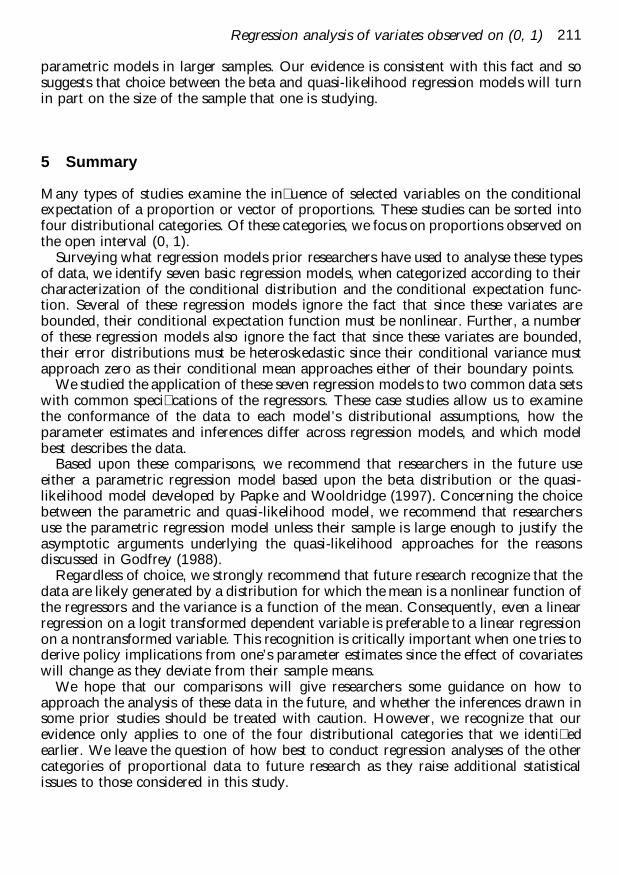
Consequently, we compare the different regression models using Akaike’s Informa-tion Criteria (AIC), as it is the most widely used and accepted model selection criteria .However, there are different variations of the AIC statistic depending upon the class ofregression models being evaluated and the sample size. We use a variation of the AICstatistic named the AICc statistic, as McQuarrie and Tsai (1998) show that it is thepreferred Kullback–Leibler information-based model selection criterion for non-normaland quasi-likelihood regression models. The AICc is de�ned as:

log(ss) ‡ n ‡ kn ¡ k ¡ 2

where log(ss) represents the natural logarithm of a regression’s mean square error, nrepresents the number of observations, and k represents the number of parameters to beestimated. Note that this measure adjusts for sample size and so is appropriate for smallas well as large samples.


An examination of Table 1 reveals that the beta regression model dominates the otherregression in terms of the AICc statistic. (The lower the value of the AICc statistic thebetter the model �t to the data. Since the number of observations and regressors are�xed across regressions in our study, this statistic will choose the regression withthe lowest mean square error.) However, the differences between the beta regressionmodel and the quasi-likelihood model are so small as to suggest that these two models�t the data equivalently well. As we show in the next case study, this last inference isdriven by sample size, and so consistent with quasi-likelihood methods being asympto-tic approximations.

4 Case study 2: Presidential voting

4.1 Description of the data

As a second case study we examine factors that in�uenced the proportion of a state’svotes for President George Bush in the 2000 Presidential Election. We obtained thevoting data from the web site www.uselectionatlas.org, which provides data on pastpresidentia l elections. We then obtained demographic, employment and income datafor each state for the year 2000 from the US Bureau of Census’ web site, fact�nder.census.gov. However, one can also obtain these data from the US Department ofAgriculture’s Economic Research Service web site, www.ers.usda.gov.

Using these data, we created the following variables. Our dependent variable is thefraction of a state’s total counted vote that was for President George Bush. Thehistogram of these data, displayed in Figure 3, clearly suggests that the data do notfollow a normal distribution. Our independent variables, or regressors, are the naturallogarithm of a state’s population (lnpop), a state’s unemployment rate (clfu), theproportion of a state’s population that a male (male), the proportion of a state’smale population that as older than 18 years of age (mgt18), the proportion of a state’spopulation that was older than 65 years (pgt65), the proportion of a state’s populationthat lived in ‘urban’ areas (urban), the proportion of a state’s households that hadannual incomes greater than $75 000 (gt75k), and �nally the proportion of a state’shouseholds whose annual income was below the ‘poverty’ level (bpovl). Using thesevariables, we estimate the following common speci�cation:

E(yjx) ˆ h(b0 ‡ b1lnpop ‡ b2clfu ‡ b3male ‡ b4mgt18 ‡ b5pgt65‡ b6urban ‡ b7gt75k ‡ b8bpovl)

We should note that we did not test to see whether this speci�cation of variables was thebest speci�cation or whether there might have been a better selection of potentialregressors. Rather, we simply chose a set of variables that seemed reasonable regressorsand used them. This approach is adequate for our purposes since we are only interestedin comparing the different regression models using a common data set and speci�cationof regressors. Nevertheless, we should note that the predictions from our nonlinear


regression models are highly correlated with actual values (around 88%). Thus ourspeci�cation has some merit.

4.2 Comparison of regression models

Our results from �tting the different regression models to the voting data are reported inTable 3. Because the patterns we observe in these data across models are so similar tothose that we observe using our cable penetration data, we will not discuss them as fullyas we did earlier. Thus, for example, we do not compute a table like Table 2, since itwould produce no new insights.

As before, we can see in Table 3 that one would be led to draw different inferencesabout which regressors were statistically signi�cant and which were not dependingupon whether one used the beta, simplex or quasi-likelihood model or one of the otherregression models. Again, as before, these differences make sense as the linear modelsfail nonlinearity tests (at the 5% level), and the residuals of regression models assuminga conditional normal distribution fail kurtosis tests of normality (at the 5% level).Consequently, we are once again able to reject the distributiona l assumptions of our�rst four regression models but not our last three regression models.

Given the similarity of evidence between these two case studies, we will focus ourattention on the computed AICc statistic for each regression model. As before, the betaregression dominates the alternatives, but it dominates the quasi-likelihood model in amore pronounced way. The fact that a parametric model, such as the beta regressionmodel, dominates the quasi-likelihood model in a smaller sample is consistent withthe fact that quasi-likelihood models are expected to be better approximations to

Figure 3 Distribution of proportion of votes going to George Bush with superimposed normal distribution


Tab

le3

Res

ult

sfo

rd

iffe

ren

tre

gre

ssio

nm

od

els

of

votin

gfo

rG

eorg

eB

ush

inth

e20

00P

resi

den

tial

elec

tion

k…x

†f…y

jx†

Lin

ear

no

rmal

Lin

ear

cen

sore

dn

orm

alT

ran

sfo

rmed

log

isti

cn

orm

alLo

gis

ticn

orm

alLo

gis

tic

bet

aLo

gis

tic

sim

ple

xLo

gis

tic

un

spec

i�ed

Est

imat

ion

met

ho

da

LSM

LLS

LSM

LM

LQ

ML

con

stan

tb¡

5.53

24**

¡5.

5324

**¡

37.5

203*

*¡

28.5

359*

*¡

38.4

671*

*¡

40.5

041*

*¡

32.8

526*

*(1

.990

9)(1

.806

7)(8

.441

9)(1

0.44

28)

(7.4

161)

(6.7

868)

(9.5

42)

lnp

op

0.01

670.

0167

0.09

28*

0.07

740.

1083

**0.

0983

**0.

0852

**(0

.011

4)(0

.010

4)(0

.048

6)(0

.050

1)(0

.041

0)(0

.042

8)(0

.045

1)cl

fu¡

2.26

08*

¡2.

2608

*¡

10.1

201*

¡9.

5962

*¡

9.83

85**

¡10

.059

6**

¡9.

8078

**(1

.320

2)(1

.198

0)(5

.597

8)(5

.526

9)(4

.134

7)(4

.395

6)(4

.502

1)m

ale

40.2

568*

*40

.256

8**

258.

553*

*19

2.69

0**

260.

816*

*27

9.49

4**

224.

048*

*(1

6.82

08)

(15.

2646

)(7

1.32

41)

(84.

1921

)(5

4.04

91)

(53.

3667

)(7

2.50

6)m

gt1

8¡

28.2

229*

*¡

28.2

229*

*¡

185.

143*

*¡

136.

255*

*¡

186.

137*

*¡

200.

541*

*¡

159.

487*

*(1

3.20

65)

(11.

9845

)(5

5.99

86)

(65.

0604

)(4

1.63

49)

(41.

8948

)(5

5.65

44)

pg

t65

¡0.

9682

*¡

0.96

82*

¡2.

6945

¡3.

5968

¡1.

7759

¡2.

2237

¡3.

1051

(0.5

611)

(0.5

092)

(2.3

792)

(2.4

339)

(2.4

892)

(2.5

229)

(2.8

105)

urb

an¡

0.00

19**

¡0.

0019

**¡

0.00

94**

¡0.

0086

**¡

0.01

01**

¡0.

0095

**¡

0.00

89**

(0.0

006)

(0.0

006)

(0.0

026)

(0.0

027)

(0.0

024)

(0.0

023)

(0.0

024)

gt7

5k¡

0.00

52¡

0.00

52¡

0.01

47¡

0.01

89¡

0.01

11¡

0.01

298

¡0.

0167

(0.0

034)

(0.0

031)

(0.0

145)

(0.0

148)

(0.0

127)

(0.0

127)

(0.0

134)

bp

ovl

0.67

540.

6754

2.82

862.

8330

2.65

862.

8266

2.83

62(0

.549

7)(0

.498

8)(2

.330

8)(2

.285

0)(1

.922

4)(1

.837

5)(1

.863

5)A

ICcc

¡1.

8038

¡1.

8038

¡4.

3387

¡4.

3538

¡4.

421

¡4.

3761

¡4.

3838

aLS

,le

ast

squ

ares

;M

L,m

axim

um

likel

iho

od

;QM

L,q

uas

i-m

axim

um

likel

iho

od

.bS

tan

dar

der

rors

are

rep

ort

edin

par

enth

eses

bel

ow

coef

�ci

ent

esti

mat

e.**

Sig

ni�

can

ceat

the

5%le

vel;

*si

gn

i�ca

nce

atth

e10

%le

vel.

c Th

isst

atis

tic

rep

rese

nts

ave

rsio

no

fth

eA

kaik

eIn

form

atio

nC

rite

ria

der

ived

inM

cQu

arri

ean

dT

sai

(199

8).


parametric models in larger samples. Our evidence is consistent with this fact and sosuggests that choice between the beta and quasi-likelihood regression models will turnin part on the size of the sample that one is studying.

5 Summary

Many types of studies examine the in�uence of selected variables on the conditionalexpectation of a proportion or vector of proportions. These studies can be sorted intofour distributiona l categories. Of these categories, we focus on proportions observed onthe open interval (0, 1).

Surveying what regression models prior researchers have used to analyse these typesof data, we identify seven basic regression models, when categorized according to theircharacterization of the conditional distribution and the conditional expectation func-tion. Several of these regression models ignore the fact that since these variates arebounded, their conditional expectation function must be nonlinear. Further, a numberof these regression models also ignore the fact that since these variates are bounded,their error distributions must be heteroskedastic since their conditional variance mustapproach zero as their conditional mean approaches either of their boundary points.

We studied the application of these seven regression models to two common data setswith common speci�cations of the regressors. These case studies allow us to examinethe conformance of the data to each model’s distributiona l assumptions, how theparameter estimates and inferences differ across regression models, and which modelbest describes the data.

Based upon these comparisons, we recommend that researchers in the future useeither a parametric regression model based upon the beta distribution or the quasi-likelihood model developed by Papke and Wooldridge (1997). Concerning the choicebetween the parametric and quasi-likelihood model, we recommend that researchersuse the parametric regression model unless their sample is large enough to justify theasymptotic arguments underlying the quasi-likelihood approaches for the reasonsdiscussed in Godfrey (1988).

Regardless of choice, we strongly recommend that future research recognize that thedata are likely generated by a distribution for which the mean is a nonlinear function ofthe regressors and the variance is a function of the mean. Consequently, even a linearregression on a logit transformed dependent variable is preferable to a linear regressionon a nontransformed variable. This recognition is critically important when one tries toderive policy implications from one’s parameter estimates since the effect of covariateswill change as they deviate from their sample means.

We hope that our comparisons will give researchers some guidance on how toapproach the analysis of these data in the future, and whether the inferences drawn insome prior studies should be treated with caution. However, we recognize that ourevidence only applies to one of the four distributiona l categories that we identi�edearlier. We leave the question of how best to conduct regression analyses of the othercategories of proportional data to future research as they raise additional statisticalissues to those considered in this study.


Acknowledgements

The authors wish to thank J Herman, J Prisbrey and D Webbink for constructivecomments on earlier drafts of this paper. The authors especially wish to thank B Marx(the editor), an anonymous associate editor and our referees for helping to improve ourpaper by their suggestions.

References

Aitchison J (1986) The statistical analysis ofcompositional data. New York, NY: Chapmanand Hall.

Albarran A, Umphrey D (1994) Marketing cableand pay cable services: impact of ethnicity,viewing motivations, and program types.Journal of Media Economics, 7, 47–58.

Atkin D (1992) A pro�le of cable subscribership:the role of audience satisfaction variables.Telematics and Informatics, 9, 53–60.

Atkinson A (1985) Plots, transformations andregression: an introduction to graphicalmethods of diagnostic regression analysis.New York: Oxford University Press.

Barclay MJ, Smith CW (1995) The determinants ofcorporate leverage and dividend policies.Journal of Applied Corporate Finance,7, 4–19.

Barndorff-Nielsen OE, Jorgensen B (1991) Someparametric models on the simplex. Journal ofMultivariate Analysis, 39, 106–16.

Cox C (1996) Nonlinear quasi-likelihood models:applications to continuous proportions.Computational Statistics & Data Analysis, 21,449–61.

Demsetz H, Lehn K (1985) The structure ofcorporate ownership: causes and consequences.Journal of Political Economy, 93,1155–77.

DeSarbo, W, Ramaswamy V, Lenk P (1993) Alatent class procedure for the structural analysisof two-way compositional data. Journal ofClassi�cation, 10, 159–93.

Dyke GV, Patterson HD (1952) Analysis offactorial arrangements when the data areproportions. Biometrics, 8, 1–12.

Fahrmeir L, Tutz G (1994) Multivariate statisticalmodelling based on generalized linear models.New York: Springer-Verlag.

Federal Communications Commission (1993) FCC93-177, Report and Order and Further Notice

of Proposed Rule Making, MM Docker 92-266(3 May 1993), 6134.

Federal Communications Commission (1994) FCC94-38, Second Order on Reconsideration,Fourth Report and Order and Fifth Notice ofProposed Rulemaking, MM Docket 92-266(30 March 1994), 4277.

Godfrey L (1988) Misspeci�cation tests ineconometrics: the Lagrange multiplier principleand other approaches. New York: CambridgeUniversity Press.

Hermalin B, Wallace N (1994) The determinantsof ef�ciency and solvency in savings andloans. The RAND Journal of Economics, 25,361–81.

Hviid M, Villadsen B (1995) Beta distributedmarket shares in a spatial model with anapplication to the market for auditservices. Review of Industrial Organization,10, 737–47.

Johnson NL, Kotz S, Balakrishnan N (1995)Continuous univariate distributions ,volumes 1 and 2. New York: John Wiley &Sons, Inc.

Jorgensen B (1983) Maximum likelihoodestimation and large-sample inference forgeneralized linear and nonlinear regressionmodels. Biometrika, 70, 19–28.

Jorgensen B (1997) The theory of dispersionmodels. New York: Chapman & Hall.

Kmenta J (1986) Elements of econometrics, 2ndedition. New York: Macmillan Publishing.

LaRose R, Atkin D (1988) Satisfaction,demographic, and media environmentpredictors of cable subscription. Journal ofBroadcasting and Electronic Media, 32,403–14.

Maddala GS (1991) A perspective on the use oflimited-dependent and qualitative variablesmodels in accounting research. The AccountingReview, 66, 786–807.


McCullagh P, Nelder JA (1989) Generalized linearmodels. New York: Chapman & Hall.

McDonald JB, Xu YJ (1995) A generalization ofthe beta distribution with applications. Journalof Econometrics, 66, 133–52.

McQuarrie A, Tsai C (1998) Regression and timeseries model selection. New Jersey: WorldScienti�c Publishing Company.

Mehran H (1995) Executive compensationstructure, ownership, and �rm performance.Journal of Financial Economics, 38, 163–84.

Mielke PW (1975) Convenient beta distributionlikelihood techniques for describing andcomparing meterological data. Journal ofApplied Meteorology, 14, 985–90.

Mittelhammer RC (1996) Mathematical statisticsfor economics and business. New York:Springer-Verlag.

Papke L, Wooldridge J (1996) Econometricmethods for fractional response variables withan application to 401(K) plan participation

rates. Journal of Applied Econometrics, 11,619–32.

Park R (1972) Prospects for cable in the 100 largesttelevision markets. Bell Journal of Economicsand Management Science, 3, 130–50.

Reagan J, Ducey R, Bernstein J (1985) Localpredictors of basic and pay cable subscription.Journalism Quarterly, 59, 397–400.

Sparkes V, Kang N (1986) Public reactions to cabletelevision: time in the diffusion process. Journalof Broadcasting, 27, 163–75.

Scott, D (1979) On optimal and data-basedhistograms. Biometrika, 66, 605–10

Titterington DM (1989) Logistic-normaldistribution. In Kotz S, Johson NL, Reed CBeds. Encyclopedia of statistical sciences(supplementary volume). New York:John Wiley & Sons, pp. 90–91.

Webb GK (1983) The economics of cabletelevision. Lexington, MA: Lexington Books.


Reproduced with permission of the copyright owner. Further reproduction prohibited without permission.

regression analysis of variates observed on (0, 1 ...bdm25/statmodelling.pdfregression analysis of...

Documents